Embed Size (px)
Citation preview

1
CITRUS ADVANCED PRODUCTION SYSTEM: UNDERSTANDING WATER AND NPK UPTAKE AND LEACHING IN FLORIDA FLATWOODS AND RIDGE SOILS
By
DAVIE MAYESO KADYAMPAKENI
A DISSERTATION PRESENTED TO THE GRADUATE SCHOOL OF THE UNIVERSITY OF FLORIDA IN PARTIAL FULFILLMENT
OF THE REQUIREMENTS FOR THE DEGREE OF DOCTOR OF PHILOSOPHY
UNIVERSITY OF FLORIDA
2012

2
© 2012 Davie Mayeso Kadyampakeni

3
To my wife Iness, son Atikonda, dad Simfoliano and mum Ernestina Kadyampakeni and my siblings Dominic, Honoratus, Felicity, Perpetual, Anthony, Auleria and Carnisius

4
ACKNOWLEDGEMENTS
First and foremost, I would like to thank the Almighty God for helping me get thus
far on the academic ladder.
In a special and grateful way, I wish to thank my co-advisors Drs. Kelly Morgan
and Peter Nkedi-Kizza for their generous financial, moral and material support. I would
like to sincerely thank them for their patience and understanding (of my personal and
professional lives) and their rare ability to combine critical evaluation of my write-ups
and/or manuscripts with warm personality and credible friendship. I feel privileged and
fortunate enough to have had the excellent opportunity to work for Dr. Morgan’s
program in Immokalee and gain hands-on experience in using advanced laboratory
equipment and software. I would like to thank Drs. Arnold Schumann, James Jawitz,
Thomas Obreza and James Jones for accepting to be on my committee and providing
material support, literature and useful suggestions for my work. Dr. Schumann is
hereby acknowledged for giving me laboratory space and all the necessary help for my
work at Lake Alfred. I would also like to thank Drs. Nkedi-Kizza, Jawitz and Jones for
their classroom instruction on Environmental Soil Physics, Contaminant Subsurface
Hydrology, and Biological and Agricultural Systems Simulation, respectively. Drs.
George O’connor, Salvador Gezan, Lawrence Winner, Allen Overman, Gregory Kiker,
Dean Rhue, William Harris, Jerry Sartain, and Samira Daroub are hereby thanked for
their classroom instruction.
I would like to thank the Southwest Florida Water Management District for
supporting this research and the Soil and Water Science Department for the matching
assistantship. I am also grateful to the sponsors of Grinter, William Robertson and Sam
Polston Graduate Fellowships and the A.S. Herlong and Doris, Earl and Verna Lowe

5
Scholarships. The help and friendship of Denise Bates, Kristy Sytsma, Janice Hill,
Kevin Hill and Julie Carson in administrative, computing technology and library and
information services at Immokalee are gratefully acknowledged for making my work a
lot easier. Rhiannon Pollard and Michael Sisk, the respective former and current
Student Services Coordinator for the Soil and Water Science Department are gratefully
recognized for their support and timely advice on paper work regarding admission,
course registration and graduation.
Dr. Monica Ozores-Hampton is also gratefully acknowledged for helping my family
settle down in Immokalee. The author recognizes the friendship and support of Drs.
Andrew Ogram (Graduate Coordinator of the Soil and Water Science Department),
Mark Rieger (Associate Dean of the College of Agricultural and Life Sciences), David
Sammons (Dean of the University of Florida International Center) and Walter Bowen
(Director of UF/IFAS International Programs).
I would like to thank the following workmates and colleagues in Gainesville for
their support in many ways: Drs. Gabriel Kasozi, Sampson Agyin-Birikorang, Nicholas
Kiggundu, Michael Miyittah, Hiral Gohil and Rajendra Paudel; Kafui Awuma, Jorge
Leiva, Augustine Muwamba, Moshik Doron, Mike Jerauld, Lucy Ngatia, Rish Prasad,
and Jongsung Kim. I am grateful to the following colleagues for their support with data
collection, laboratory procedures, use of software and other equipments at Immokalee
and Lake Alfred: Drs. Shinjiro Sato, Kamal Mahmoud and Kiran Mann; Laura Waldo,
Smita Barkataky, Wafaa Mohamoud, Assma Zekri, Ann Summerals and Shengsen
Wang. My friends at Immokalee Melissa Benitez, Sunehali Sharma and Utpal Handque
are also thanked for their friendship and help.

6
I cherish the friendship and support of my fellow Malawian students who pursued
various graduate programs at UF: Bonet Kamwana, Innocent Thindwa, Pearson Soko,
Fiskani Nkana, Lucy Nyirenda, Jonathan Chiputula, Wycliffe Kumwenda, Aubrey
Chinseu, Matrina Soko, Felix Makondi, Hamie Chakana, Chunala Njombwa, Suzgo
Chapa and Donald Kazanga. The families of Dr. Nkedi-Kizza, Dr. Chikagwa-Malunga
and Dr. Lergo are thanked for their friendship and company.
My friend Thomson Paris, his dad Trevor, mum Cindy, brother Taylor and sister
Sarah are thanked for being materially, spiritually, financially and morally so supportive
to me and my family. I have vivid memories of my time in Jacksonville, St. Augustine,
Chatanooga, Baltimore and Washington D.C. I am also grateful to Scott Croxton and his
mum for their friendship and support.
Over and above all, I would like to recognize and thank my wife, Iness and son,
Atikonda for their company and incessant support during the final and most demanding
times of my graduate program. My dad Simfoliano and mum Ernestina Kadyampakeni,
my mother-in-law Martha Mhango and my siblings Dominic, Honoratus, Felicity,
Perpetual, Anthony, Auleria and Carnisius; my in-laws and many nephews and nieces,
my uncles and aunts and cousins have always inspired and sustained my urge for
higher academic accomplishment and professional advancement through their prayers,
advice and encouragement.

7
TABLE OF CONTENTS
page
ACKNOWLEDGEMENTS ............................................................................................... 4
LIST OF TABLES .......................................................................................................... 11
LIST OF ABBREVIATIONS ........................................................................................... 17
ABSTRACT ................................................................................................................... 20
CHAPTER
1 INTRODUCTION .................................................................................................... 22
Justification for Research on Citrus Irrigation and Nutrient Management in Florida.................................................................................................................. 24
Soil Types in Florida’s Citrus Growing Regions ................................................ 24 Climate ............................................................................................................. 25 Citrus Canker and Greening Diseases ............................................................. 26
Planting Densities ............................................................................................. 28 Citrus Root Length Density ............................................................................... 28
Overview of the Dissertation ................................................................................... 29 General Research Goals and Hypotheses .............................................................. 31 Summary ................................................................................................................ 32
2 LITERATURE REVIEW .......................................................................................... 34
The Open Hydroponic System and Advanced Production Systems ....................... 35
Concepts .......................................................................................................... 35 Maximize water and nutrient efficiency ...................................................... 35
Concentrate roots in irrigated zone ............................................................ 36 Reduce nutrient leaching ........................................................................... 37 Applications of OHS in view of Florida’s soil types and current BMPs ....... 37
Tree density ............................................................................................... 39 Tree size control with rootstocks ................................................................ 39
Fertilizer Demand and Nutrient Uptake in Citrus ..................................................... 40 Biomass Development with Time ..................................................................... 40
Nutrient Requirements for Biomass and Fruit Production ................................ 42 Nutrient Uptake and Nutrient Use Efficiency ........................................................... 48
Citrus Nutrient Management ............................................................................. 48 Extraction Methods for N-Forms, P, and K from Soils and Plant Tissue .......... 49
Irrigation Design and Scheduling-Drip and Microsprinkler Irrigation ....................... 52
Evapotranspiration Calculations ....................................................................... 52 Citrus Crop Coefficients.................................................................................... 54
Water Use Efficiency ........................................................................................ 54

8
Bromide as a Tracer for Water Movement in the Soil ....................................... 55
Irrigation Methods ............................................................................................. 56 Irrigation Control Methods ................................................................................ 57
Citrus Root Density Distribution ........................................................................ 57 Process-Oriented Models for Solute Transport, Water and Nutrient Uptake........... 59
Types and Use of Models in Agriculture ........................................................... 59 Comparing Soil Water and Hydrologic Models ................................................. 61 Models Used for Citrus Production ................................................................... 62
Summary ................................................................................................................ 63
3 NUTRIENT UPTAKE EFFICIENCY AND DISTRIBUTION IN-SITU FROM THE CITRUS ROOT ZONE ............................................................................................ 68
Materials and Methods............................................................................................ 70
Site Conditions ................................................................................................. 70 Study Treatments and Experimental Design .................................................... 70
Plant Tissue and Soil Sampling Design and Analytical Methods ...................... 71 Soil sampling .............................................................................................. 71
Water sample collection and processing .................................................... 72 Extraction of NH4-N, NO3-N, P, Br and K ................................................... 73 Analysis of soil extracts and water samples ............................................... 74
Plant tissue sampling and analysis ................................................................... 74 Leaf sampling ............................................................................................. 74
Destructive tree sampling and tissue processing ............................................. 75 Tissue analysis .......................................................................................... 76
Quality Control of Plant Tissue and Soil Sample Analysis ................................ 76
Data Analysis ................................................................................................... 77 Results and Discussion........................................................................................... 77
Leaf NPK Concentration as a Function of Irrigation System............................. 77 NPK Distribution in the Citrus Root Zone as a Function of Time, Depth and
Lateral Distance ............................................................................................ 78 N, P, Br and K Leaching in the Irrigated and Nonirrigated Zones ..................... 83 Water Quality Analysis ..................................................................................... 89
Biomass and Nutrient Distribution as a Function of Irrigation Practice ............. 90 Summary ................................................................................................................ 92
4 EFFECTS OF FERTIGATION AND IRRIGATION RATES ON ROOT LENGTH DISTRIBUTION AND TREE SIZE ........................................................................ 122
Materials and Methods.......................................................................................... 125 Description of Study Sites and Treatments .................................................... 125 Root Sampling Methods ................................................................................. 126 Estimation of Tree Growth Characteristics ..................................................... 127 Statistical Analysis .......................................................................................... 127
Results and Discussion......................................................................................... 128 Correlation of RLD Measured by Intersection Method versus Scanning
Method ........................................................................................................ 128

9
RLD Distribution as a Function of Irrigation Method, Time and Soil Depth ..... 129
Effect of Fertigation Method on Trunk Cross-Sectional Area and Canopy Volume ........................................................................................................ 134
Summary .............................................................................................................. 135
5 EFFECTS OF IRRIGATION METHOD AND FREQUENCY ON CITRUS WATER UPTAKE AND SOIL MOISTURE DISTRIBUTION .................................. 147
Materials and Methods.......................................................................................... 150 Experimental design and irrigation methods................................................... 150
Estimation of Soil Moisture ............................................................................. 150 Estimation of Crop Water Uptake and Kc........................................................ 151
Results and Discussion......................................................................................... 153 Tree characteristics at Immokalee and Lake Alfred ........................................ 153
Water Uptake at Immokalee and Lake Alfred ................................................. 154 Soil moisture distribution at Lake Alfred and Immokalee ................................ 161
Factors affecting water uptake on the two soils .............................................. 164 Summary .............................................................................................................. 165
6 CALIBRATION AND VALIDATION OF WATER, N, P, BR AND K MOVEMENT ON A FLORIDA SPODOSOL AND ENTISOL USING HYDRUS-2D .................... 194
Materials and Methods.......................................................................................... 195
Governing Equations and Parameters for Water Flow, Nutrient Transport and Uptake .................................................................................................. 195
Model Calibration Processes .......................................................................... 198
Sorption isotherms determination ............................................................ 198
Determination of soil water retention and hydraulic functions .................. 200 Sensitivity Analysis of Selected Parameters for HYDRUS-2D ........................ 203 Simulation Domain-Microsprinkler irrigation ................................................... 206
Simulation Domain-Drip irrigation ................................................................... 206 Results and Discussion......................................................................................... 207
Sensitivity analysis and calibration of selected model parameters ................. 207 Water, Br, K, P, NO3 and NH4 movement with drip and microsprinkler
irrigation ...................................................................................................... 208
Phosphorus movement with microsprinkler irrigation as function of KD value 209 Investigating bromide, nitrate and water movement using weather data from
Immokalee and Lake Alfred. ........................................................................ 210 Summary .............................................................................................................. 211
7 CONCLUSIONS ................................................................................................... 228
APPENDIX
A SUPPLEMENTARY FIGURES TO CHAPTERS 3, 4 AND 5 ................................ 234
B CHARACTERIZATION OF SORPTION ISOTHERMS FOR AMMONIUM-N, K AND P ON THE FLATWOODS AND RIDGE SOILS ............................................ 278

10
C SOIL WATER CHARACTERISTIC CURVES AND HYDRAULIC FUNCTIONS ... 289
D SCHEMATIC FIELD DIAGRAMS SHOWING THE SET-UP OF DRIP AND MICROSPRINKLER IRRIGATION SYSTEMS ...................................................... 296
E AVERAGE MONTHLY TEMPERATURE, RELATIVE HUMIDITY, RAINFALL, SOLAR RADIATION AND EVAPOTRANSPIRATION ......................................... 304
F CORRELATIONS BETWEEN RLD MEASURED BY LINE INTERSECTION METHOD AND PREDICTED RLD BY SCANNING METHOD AND SCANNED AREA .................................................................................................................... 306
G EXPERIMENTAL SET UP FOR THE SORPTION STUDY ................................... 314
H SORPTION COEFFICIENTS FOR NH4+ AND K+ ON IMMOKALEE AND
CANDLER FINE SAND USING FERTILIZER MIXTURE IN TAP WATER ........... 315
I SORPTION COEFFICIENTS FOR P ON IMMOKALEE AND CANDLER FINE SAND .................................................................................................................... 316
LIST OF REFERENCES ............................................................................................. 317
BIOGRAPHICAL SKETCH .......................................................................................... 344

11
LIST OF TABLES
Table page 2-1 Typical percent biomass distribution (dry weight basis) in oranges from
different parts of the world .................................................................................. 65
2-2 Typical nutrient uptake rates in oranges ............................................................. 66
2-3 Soil test interpretation for soil P extraction methods compared with Mehlich 1 extractant§ .......................................................................................................... 67
2-4 Guidelines for interpretations of orange tree leaf analysis based on 4 to 6-month-old spring flush leaves from non-fruiting twigs¶........................................ 67
3-1 2M KCl extractable NH4+-N and NO3--N, M1K and M1P concentrations of soil
samples collected in June 2009 at SWFREC ..................................................... 98
3-2 2M KCl extractable NH4+-N and NO3--N, M1K and M1P concentrations of soil
samples collected in August 2009 at SWFREC .................................................. 99
3-3 2M KCl extractable NH4+-N and NO3
--N, M1K and M1P concentrations of soil samples collected in June 2010 at SWFREC ................................................... 100
3-4 2M KCl extractable NH4+-N and NO3
--N, M1K and M1P concentrations of soil samples collected in December 2009 at the Lake Alfred site ........................... 101
3-5 2M KCl extractable NH4+-N and NO3
--N, M1K and M1P concentrations of soil samples collected in July 2010 at the Lake Alfred site ..................................... 102
3-6 Fresh and dry tissue weight for samples collected in July 2011 at Immokalee . 117
3-7 Fresh and dry tissue weight for samples collected in August 2011 at the Lake Alfred site ......................................................................................................... 118
3-8 N, P and K concentration in tissues collected in July 2011 at the Immokalee site .................................................................................................................... 119
3-9 N, P and K concentration in tissues collected in August 2011 at the Lake Alfred site ......................................................................................................... 119
3-10 Nitrogen, phosphorus and potassium accumulation on Immokalee sand ......... 120
3-11 N, P and K accumulation in 2011 at the Lake Alfred and Immokalee sites ....... 121
4-1 Models for RLD estimation at CREC ................................................................ 137
4-2 Models for RLD estimation at SWFREC ........................................................... 138

12
4-3 RLD as a function of irrigation method, soil depth and distance from the tree at SWFREC in June 2009 ................................................................................ 139
4-4 RLD as a function of irrigation method, soil depth and distance from the tree at SWFREC in June 2010 ................................................................................ 140
4-5 RLD as a function of irrigation method, soil depth and distance from the tree at the Lake Alfred site in December 2009 ......................................................... 141
4-6 RLD as a function of irrigation method, soil depth and distance from the tree at the Lake Alfred site in July 2010 ................................................................... 142
4-7 Trunk cross-sectional area as function of fertigation method at the Lake Alfred site ......................................................................................................... 146
5-1 Average leaf area ............................................................................................. 167
5-2 Tree canopy volume (CV), stem cross-sectional area (SCA), and trunk cross-sectional area (TCA) ......................................................................................... 167
5-3 Linear regression models relating cumulative water uptake to tree and soil characteristics at the Lake Alfred site in July 2010 and September 2011† ....... 192
5-4 Multiple linear regression model coefficients for cumulative water uptake ....... 193
6-1 Selected parameters for sensitivity analysis for simulating water flow and nutrient movement in citrus using HYDRUS-2D ............................................... 215
6-3 Simulation experiment scenarios for the Ridge and Flatwoods soils ................ 217
6-4 Soil physical characteristics and initial conditions of the Immokalee and Candler fine sands ............................................................................................ 217
6-5 Sensitivity indices for selected parameters for soil available water, P, ammonium and K movement using HYDRUS-2D ............................................ 218
6-6 Statistical comparison between the observed and simulated water contents in spring and summer on Candler and Immokalee sand ...................................... 225
6-7 Statistical comparison between the observed and simulated Br, NO3, NH4, M1P and M1K on Candler and Immokalee sand .............................................. 226

13
LIST OF FIGURES Figure page 1-1 Typical soil orders of Florida ............................................................................... 33
3-1 Destructive tree sampling in July 2011 at Immokalee with the root zone of the tree marked to 30-cm depth................................................................................ 95
3-2 Leaf NPK concentration determined in June 2009 at Immokalee ....................... 96
3-3 Leaf NPK concentration determined in August 2011 at the Lake Alfred site ...... 97
3-4 Lateral ammonium N distribution at 0-30 cm soil depth in June 2009 and 2010 at the Immokalee site............................................................................... 103
3-5 Lateral nitrate N distribution in June 2009 and 2010 at Immokalee site ........... 104
3-6 Lateral ammonium N distribution in December 2009 on Candler fine sand ...... 105
3-7 Lateral ammonium N distribution in July 2010 at the Lake Alfred site .............. 106
3-8 Lateral nitrate N distribution in December 2009 at the Lake Alfred site ............ 107
3-9 Lateral nitrate N distribution in July 2010 at the Lake Alfred site ...................... 108
3-10 Lateral Mehlich 1 P distribution at Immokalee site in June 2009 and 2010 ...... 109
3-11 Lateral Mehlich 1 P distribution in the 0-30 cm depth layer at the Lake Alfred site in December 2009 ...................................................................................... 110
3-12 Lateral Mehlich 1 P distribution in the 0-30 cm depth layer at the Lake Alfred site in July 2010 ................................................................................................ 111
3-13 Lateral Mehlich 1 K distribution at Immokalee in June 2009 and 2010 ............. 112
3-14 Lateral Mehlich 1 K distribution at the Lake Alfred site in December 2009 ....... 113
3-15 Lateral Mehlich 1 K distribution at the Lake Alfred site in July 2010 ................. 114
3-16 Vertical nitrate N and ammonium N distribution in June 2010 at Immokalee site and in July 2010 at the Lake Alfred site ..................................................... 115
4-1 Canopy volume as a function of fertilization practice at the Lake Alfred site. ... 143
4-2 Trunk cross-sectional area as a function of fertigation practice at the Immokalee site. ................................................................................................ 144
4-3 Canopy volume as a function of fertigation method at the Immokalee site ....... 145

14
5-1 Linear correlations of leaf area index and canopy volume as a function of leaf area in March 2011 at the Lake Alfred site ....................................................... 168
5-2 Correlations of leaf area index and canopy volume as a function of total leaf area at Immokalee site in March 2011 .............................................................. 169
5-3 Average hourly sap flow in July, 2010 and March, 2011 at Lake Alfred site ..... 170
5-4 Average daily sap flow in July, 2010 at the Lake Alfred site ............................. 171
5-5 Average daily sap flow in March, 2011 at the Lake Alfred site ......................... 171
5-6 Average hourly sap flow in February-March 2011 at SWFREC. ....................... 172
5-7 Average daily sap flow in February-March 2011 at SWFREC. ......................... 173
5-8 Average hourly flow in June 2011 at the Immokalee site .................................. 174
5-9 Average hourly sap flow in August-September, 2011 at the Lake Alfred site ... 175
5-10 Average daily sap flow in June 2011 at the Immokalee site ............................. 176
5-11 Average daily sap flow in August-September, 2011 at the Lake Alfred site ...... 177
5-12 Average hourly soil moisture distribution in July 2010 at the Lake Alfred site measured at 10- and 45 cm soil depth layers ................................................... 178
5-13 Average daily soil moisture distribution in July 2010 at the Lake Alfred site measured at 10 cm soil depth layer .................................................................. 179
5-14 Soil moisture distribution in July 2010 at the Lake Alfred site measured at 45 cm soil depth layer ............................................................................................ 179
5-15 Average hourly soil moisture distribution at the Lake Alfred site measured at 10 cm (top) and 45 cm (bottom) soil depth layers in March 2011. .................... 180
5-16 Daily soil moisture distribution at the Lake Alfred site measured at 10 cm soil depth layer in March 2011 ................................................................................ 181
5-17 Daily soil moisture distribution at the Lake Alfred site measured at 45 cm soil depth layer in March 2011 ................................................................................ 181
5-18 Average hourly soil moisture distribution at the Lake Alfred site measured at 10- and 45 cm soil depth layers in August-September 2011 ............................ 182
5-19 Average daily soil moisture distribution at the Lake Alfred site measured at 10 cm soil depth layer in August-September 2011 ........................................... 183

15
5-20 Average daily soil moisture distribution at the Lake Alfred site measured at 45 cm soil depth layer in August-September 2011 ........................................... 184
5-21 Soil moisture distribution for DOHS in February-March 2011 at Immokalee site measured at 10-, 20-, 30-, 40- and 50 cm soil depth layers ....................... 185
5-22 Soil moisture distribution for DOHS in June 2011 at Immokalee site measured at 10-, 20-, 30-, 40- and 50 cm soil depth layers. ............................ 186
5-23 Soil moisture distribution for MOHS in February-March 2011 at Immokalee site measured at 10-, 20-, 30-, 40- and 50 cm soil depth layers ....................... 187
5-24 Soil moisture distribution for MOHS in June 2011 at Immokalee site measured at 10-, 20-, 30-, 40- and 50 cm soil depth layers ............................. 188
5-25 Soil moisture distribution for CMP in February-March 2011 at Immokalee site measured at 10-, 20-, 30-, 40- and 50 cm soil depth layers ............................. 189
5-26 Soil moisture distribution for CMP in June 2011 at Immokalee site measured at 10-, 20-, 30-, 40- and 50 cm soil depth layers .............................................. 190
5-27 Correlation of water uptake and canopy volume at the Immokalee and Lake Alfred sites ........................................................................................................ 191
6-1 A forrester diagram describing the conceptual model for water and nutrient uptake and movement processes ..................................................................... 213
6-2 Calibration of HYDRUS-2D for simulating soil water content at 10 cm soil depth at Lake Alfred site using drip irrigation .................................................... 214
6-3 Calibration of HYDRUS-2D for simulation soil water content at 40 cm soil depth at Lake Alfred site using microsprinkler irrigation ................................... 214
6-4 Calibration of HYDRUS model for simulating ammonium N movement on Candler fine sand ............................................................................................. 215
6-5 Soil Br monitored at 15- and 60 cm depth using drip irrigation at the Lake Alfred site ......................................................................................................... 219
6-6 Measured and simulated Br concentration at 15 and 60 cm at Immokalee site using microsprinkler irrigation ........................................................................... 220
6-7 Soil P monitored at 15 cm depth using drip irrigation at the Lake Alfred site .... 221
6-8 Simulated and measured cumulative nitrate concentration using microsprinkler irrigation at the Immokalee site.................................................. 221
6-9 Simulated and measured cumulative ammonium concentration using drip irrigation at the Immokalee site ......................................................................... 222

16
6-10 Cumulative K distribution at 15 cm soil depth at Immokalee site using microsprinkler irrigation .................................................................................... 223
6-11 Cumulative K distribution at 15 cm soil depth at Immokalee site using drip irrigation ............................................................................................................ 223
6-12 Phosphorus movement on Candler and Immokalee fine sand depending on KD value estimated using HYDRUS-1D ............................................................ 224
6-13 Simulated nitrate, bromide and water movement over a 90 day period at 60 cm using grower practice .................................................................................. 227

17
LIST OF ABBREVIATIONS
AB-DTPA Ammonium bicarbonate-diethylenetriamine pentaacetic acid
ACPS Advanced Citrus Production Systems
ANOVA Analysis of Variance
ARS Agricultural Research Service
ASWD Available soil water depletion
BMP Best Management Practice
CDE Convection-Dispersion Equation
CEC Cation Exchange Capacity
CMP Conventional Microsprinkler Practice
CREC Citrus Research and Education Center
CWMS Citrus Water Management System
DM Dry matter
DMRT Duncan Multiple Range Test
DOHS Drip Open Hydroponics System
DSSAT Decision Support System for Agrotechnology Transfer
DW Dry weight
ER Effective rainfall
Esap Daily sapflow per unit land area
ET Evapotranspiration
ETo Reference evapotranspiration
FRLD Fibrous root length density
FW Fresh weight

18
GLM General Linear Model
GSA Global Sensitivity Analysis
HLB Huanglongbing
ICP Inductively Coupled Plasma
ICP-AES Inductively Coupled Plasma Atomic Emission Spectrometry
IFP Intensive Fertigation Practice
Kc Crop coefficient
LAI Leaf Area Index
LEACHM Leaching and Chemistry Model
M1K Mehlich 1 extractable potassium
M1P Mehlich 1 extractable phosphorus
MOHS Microsprinkler Open Hydroponics System
NCSWAP Nitrogen, Carbon, Soil, Water and Plant
OHS Open Hydroponics System
NPV Net Present Value
RAW Readily available water
RLD Root length density
RZWQM Root Zone Water Quality Model
SHB Stem-heat balance
SWASIM Soil Water Simulation Model
SWATRE Soil Water and Actual Transpiration, Extended
SWFREC Southwest Florida Research and Education Center
TAW Total available water

19
TCA Trunk cross-sectional area
TSS Total Soluble Solids
UF Upflux
UF/IFAS University of Florida/Institute of Food and Agricultural Sciences
USA United States of America
USDA United States Department of Agriculture
20
Abstract of Dissertation Presented to the Graduate School of the University of Florida in Partial Fulfillment of the Requirements for the Degree of Doctor of Philosophy
CITRUS ADVANCED PRODUCTION SYSTEM: UNDERSTANDING WATER AND NPK
UPTAKE AND LEACHING IN FLORIDA FLATWOODS AND RIDGE SOILS
By
Davie Mayeso Kadyampakeni
August 2012
Chair: Kelly T. Morgan Cochair: Peter Nkedi-Kizza Major: Soil and Water Science
Florida citrus production is ranked number one in the nation, accounting for 63% of
the 371,700 ha production area in the U.S. California, Texas, and Arizona account for
32.5%, 3.3% and 1.6%, respectively. Citrus production in Florida has declined over the
past 14 years from 342,077 ha in 1998 to 232,470 ha in 2011 largely due to increased
urbanization, hurricanes, citrus canker (Xanthomonas axonopodis) and citrus greening
(Liberibacter asiaticus). The uneven rainfall distribution and sandy soils make water
and nutrient management extremely difficult. Thus, novel practices termed advanced
citrus production systems (ACPS) using higher tree density, dwarfing rootstocks and a
modified open hydroponics system (OHS) were developed to accelerate tree growth
and bring young trees into production so growers can break-even within a few years of
establishing a grove. Several field and laboratory experiments coupled with computer
simulations were conducted to compare the performance of the intensively managed
drip and microsprinkler irrigation and fertigation systems with conventional grower
practices on the Florida Flatwoods and Ridge soils.

21
The Ridge and Flatwoods field studies revealed higher but not significantly
different water uptake with ACPS/OHS compared with grower practices. However,
tissue nutrient concentration was greater for ACPS/OHS than the grower practices. In
addition, ACPS/OHS practices, particularly on the Ridge, increased soil nutrient
retention in the root zone by 60-90% compared with conventional fertigation or granular
fertilization. The soil cores indicated greater root length density for ACPS/OHS than
grower practice, in the irrigated zones, and in the 0-15 cm soil layer. HYDRUS-2D
model, calibrated with field and laboratory data, showed reasonably good agreements
between simulated and measured values suggesting that HYDRUS-2D could
successfully be used as a tool for irrigation and nutrient management decision support.
Overall, the results underline the importance of using innovative and carefully
managed intensive fertigation practices in promoting tree growth and root length
density, increasing nutrient and water uptake, and conserving environmental quality
while sustaining high citrus yields on Florida’s sandy soils. The results from the field
experiments and computer simulations should allay any fears of potential groundwater
contamination associated with proper use of the ACPS/OHS practices.

22
CHAPTER 1 INTRODUCTION
Citrus is one of the most important crops in Florida with an annual value of $1.1
billion dollars (USDA, 2011). In 2010, Florida ranked number one in the nation for citrus
production, accounting for 63% of the 371,700 ha production area in the U.S., while
states of Arizona, Texas and California accounted for 6,075 ha, 12,285 ha and 120, 870
ha, respectively. At a global scale, the U.S. produced 12% of the 83 million ton world
citrus production in 2010 (USDA, 2011).
Research data from several studies show that increasing water costs and
environmental concerns create a need for more efficient management practices for
citrus production (Lamb et al., 1999; Alva et al., 2003; Paramasivam et al., 2000a; 2001;
Alva et al., 2006a, b). Irrigating to meet crop evapotranspiration (ET) demand and
fertigation at optimal nutrient levels have the potential to increase production efficiency.
The modifications to current irrigation water and nutrient management
recommendations are termed open hydroponics system (OHS) and advanced citrus
production systems (ACPS). OHS is an integrated system of irrigation, nutrition and
horticultural practices that was developed in Spain to improve production on gravel
based soils with low fertility (Martinez-Valero and Fernandez, 2004; Falivene et al.,
2005). According to Stover et al. (2008), OHS provides tight control over water and
nutrient-mediated plant growth and development using irrigation to train the root system
into a limited area and fertigates with daily nutrient requirements. The ACPS is a short-
to medium-term approach to citrus water and nutrient management being evaluated in
Florida citrus groves for sustainable, profitable citrus production in the presence of
greening and canker diseases with the goal of compressing and enhancing the citrus

23
production cycle so economic payback can be reached in fewer years to offset some of
the disease losses (Schumann et al., 2009). Elements of OHS that have been
incorporated into an Advanced Citrus Production System (ACPS) include a) intensive
daily fertigation with complete balanced nutrient formula for early high yields and control
of shoot and root growth; 2) high density planting to enable early high yields and early
return to investment, and 3) a suitable rootstock adaptable to close spacing and
intensive fertigation, capable of promoting vigorous tree growth and high root density in
the fertigated zone (Morgan et al., 2009b).
Muraro (2008) described the costs associated with shifting from current production
systems to ACPS/OHS. The added costs to establish an ACPS/OHS with 890 trees ha-1
are about $13,541 ha-1 more than if a block is replanted to a more typical density of 371
trees ha-1 owing to buying 519 additional trees ha-1, planting costs, irrigation/bed
preparation and young tree management (Muraro, 2008; Roka et al., 2009). However,
net present value (NPV) analysis performed by Roka et al. (2009) over a 15-year
horizon and a constant delivered-in price of $1.20 per pound-solids, showed a
cumulative NPV of $7,949 ha-1 for 890 trees ha-1 planting and a negative ($833) ha-1 for
a 371 trees ha-1 planting. The higher returns from ACPS affords a grower a greater
cushion against low market prices than a 371 trees ha-1 planting. Thus enhancing
production from young trees carries two benefits: 1) sustained higher fruit yield over
time, and 2) increasing net returns earlier in the cashflow stream when discount rates
are relatively higher (Roka et al., 2009).
Despite these postulated notions, research studies on the effect of irrigating at
various ET levels and specific NPK levels using OHS on the productivity of young citrus

24
trees have not been adequately conducted on Florida Flatwoods and Ridge soils. This
is key to understanding, in detail, interacting factors and processes that govern citrus
water and nutrient uptake and movement of nutrients such as N, P and K in the citrus
root zone. Also, use of the OHS for fertilizer management in citrus production on
Florida soils with high percentage of sand (>85%) and low organic matter content (<2%)
may further reduce nutrient leaching and subsequent pollution of groundwater.
This study hypothesizes that proper scheduling of irrigation water by drip or
microsprinkler using OHS will improve water and nutrient use efficiency thus helping
farmers more efficiently manage inputs in an ecologically sound manner, and attain high
citrus growth and/or yields.
For optimum citrus tree growth and yield, fertilization rate and timing must be
accompanied by efficient water management to avoid leaching of nutrients below the
root zone thus increasing nutrient use efficiency. The research objectives of the studies
in the following chapters focus on 1) improved crop growth and fertilizer use efficiency,
2) irrigation management optimization, and 3) modeling of soil-fertigation interactions
with the goals of (1) realizing lower water and fertilizer use, (2) ensuring sustainable
citrus yields and (3) avoiding environmental pollution associated with nutrient leaching
from the citrus root-zone (Morgan and Hanlon, 2006).
Justification for Research on Citrus Irrigation and Nutrient Management in Florida
Soil Types in Florida’s Citrus Growing Regions
Most Florida citrus is grown on sandy soils that are unable to retain more than a
minimal amount of soluble plant nutrients against leaching by rainfall or excessive
irrigation (Obreza and Collins, 2008). Typical soil orders in the Florida citrus producing
regions are Entisols on the Florida Ridge and Spodosols and Alfisols in the Flatwoods

25
(Figure 1-1). Entisols, found mostly in central Florida, are characterized by excessive
drainage, good aeration and a deep root zone (Alva et al., 1998; Fares and Alva, 1999;
2000a, b; Morgan et al., 2006b; Fares et al., 2008; Obreza and Collins, 2008). These
soils are ascribed to high hydraulic conductivity for Entisols ranging from 15-215cm h-1
with percentage sand >95% (Paramasivam et al., 2001; 2002; Obreza and Collins,
2008). In the Flatwoods, the Alfisols (except Winder soil series that has 85% sand) and
Spodosols contain about 94-98% sand in the top 45cm making irrigation water and
nutrient management extremely difficult (Obreza and Collins, 2008). Generally, these
soils have low water holding and nutrient retention capacity due to the sandy soil
characteristic and low organic matter and thus require use of intensive and well-
managed irrigation and fertigation systems that promote high water- and nutrient-use
efficiency for high citrus yields.
Climate
Citrus trees in Florida must be irrigated to reach maximum production owing to
uneven rainfall distribution and low soil water-holding capacity (Morgan et al., 2006b).
However, citrus irrigation and crop water requirements vary with climatic conditions and
variety (Rogers and Barholic, 1976; Boman, 1994; Fares and Alva, 1999). Florida citrus
water requirement is reported to range from 820 to 1280 mm yr-1 (Rogers et al., 1983)
while 60% of the average annual rainfall (approximately 1386 mm) is distributed in the
summer months of May through August (Paramasivam et al., 2001; Obreza and Pitts,
2002; Paramasivam et al., 2002). Thus, the rain is not distributed uniformly throughout
the year stressing the need for supplementary irrigation.

26
Citrus Canker and Greening Diseases
According to USDA (2011), citrus production in Florida decreased from 386,137 ha
in 1966 to 249,317 ha in 2010, as a result of increased urbanization, hurricanes, citrus
canker (Xanthomonas axonopodis) and citrus greening (Liberibacter asiaticus). The
latter two diseases have eliminated 10 to 30% of trees and reduced yields of other trees
in some citrus groves in Florida (Gottwald et al., 2002a, b; Irey et al., 2008). In a study
on the spread of citrus greening (also called Huanglongbing (HLB)) in Florida,
Manjunath et al. (2008) found that 9% of plant samples from 43 different counties tested
positive for Liberibacter asiaticus.
Citrus bacterial canker disease is a quarantine pest for many citrus growing
countries (Gottwald et al., 2002a). Citrus canker occurs primarily in tropical and
subtropical climates where considerable rainfall accompanies warm temperatures as is
the case with Florida (Polex et al., 2007). The disease is exacerbated when wet
conditions occur during periods of shoot emergence and development of young citrus
fruit (Halbert and Manjunath, 2004; Polex et al., 2007). Citrus canker is mainly leaf-
spotting and rind-blemishing disease characterized by defoliation, shoot dieback and
fruit drop (Polex et al., 2007) and currently managed through eradication and exclusion
of infected and exposed trees (Gottwald et al., 2002b).
Citrus greening (also called Huanglongbing (HLB)) is a disease caused by several
species of Candidatus Liberibacter consisting of phloem-limited, uncultured bacteria
(Zhao, 1981; da Graca and Korsten, 2004. HLB in Florida, vectored by the Asian psyllid
(Diaphorina citri) (Zhao, 1981), mostly likely originated in China, where it was given its
name because of its characteristic symptom, a yellowing of the new shoots in the green
canopy (Polex et al., 2007). There is no cure for the infected trees which decline and

27
die within a few months or years (Chung and Brlansky, 2009). The fruit produced by the
infected trees is not suitable for the fresh market or juice processing due to significant
increase in acidity and bitter taste (Polex et al., 2007; Chung and Brlansky, 2009). HLB
bacteria can infect most citrus cultivars, species, and hybrids as well as some citrus
relatives (Halbert and Manjunath, 2004). Chronically infected trees display extensive
twig and limb dieback, tend to drop fruit prematurely, and are sparsely foliated with
small leaves that point upward (Bove, 2006; Polex et al., 2007). HLB-infected fruits are
frequently small, underdeveloped and misshapen (Polex et al., 2007). Management of
HLB disease has proven to be very difficult, as a result, there are no cases of a
completely successful eradication program to date (da Graca and Korsten, 2004;
Halbert and Manjunath, 2004; Chung and Brlansky, 2009). Bove (2006) recommended
the elimination of Liberibacteria inoculum by removing infected trees, keeping psyllid
populations as low as possible through use of contact and systemic insecticides, the
use of healthy material for replanting and introduction of biological control predators.
Bove (2006) estimated that an orchard with 30% symptomatic trees, half of the trees are
infected and will have to be pulled out sooner or later. Also, surveys conducted over an
8-year period in Reunion Island indicated that 65% of the trees were badly damaged
and rendered unproductive within 7 years after planting (Aubert et al., 1996). In
Thailand, citrus trees generally decline within 5-8 years after planting due to citrus
greening, and yet, groves must be maintained for a minimum of 10 years in order to
make a profit (Roistacher, 1996).
The use of ACPS is an attempt to help growers optimize production in the face of
the impact of canker and greening diseases on tree health and yields. One strategy

28
being proposed is the use of intensive nutrient management to accelerate tree growth
and bring young trees into production so growers can break-even within a few years of
establishing a grove (Stover et al., 2008; Morgan et al., 2009b; Schumann et al., 2009).
Planting Densities
In Florida, studies on citrus tree densities have been done over the years and
show that high planting density produced higher yields (Castle, 1980; Whitney and
Wheaton, 1984; Parsons and Wheaton, 2009) and utilized nutrients and irrigation water
more efficiently (Parsons and Wheaton, 2009). However, most of the studies done in
Florida used much lower densities (80-200 trees per acre) (Obreza, 1993; Obreza and
Rouse, 1991; 1993; Alva and Paramasivam, 1998; Paramasivam et al., 2000b) and
standard granular fertilization practice or infrequent fertigation at 112-280 kg N ha-1 yr-1
(Paramasivam et al., 2000b; 2001; 2002) than the 250 trees or more per acre and very
frequent fertilization practices proposed for OHS (Stover et al., 2008; Morgan et al.,
2009b; Schumann et al., 2009).
Citrus Root Length Density
Citrus root length density is a critical indicator of the potential for water and
nutrient uptake. Studies on root water and nutrient uptake are better described with root
length density (Morgan et al., 2006b; 2007). Several researchers observed that roots of
trees grown in the Flatwoods display much stronger lateral than vertical development
(Reitz and Long, 1955; Calvert et al., 1977; Bauer et al., 2004). Research on root
length density (RLD) distribution has never been conducted on OHS/ACPS. The RLD
data discussed in subsequent chapters will help define the potential of OHS/ACPS in
promoting tree water and nutrient uptake while helping retain nutrients and water in the
root zone.

29
Overview of the Dissertation
In view of the need for research on citrus irrigation and nutrient management to
reduce the impact of greening infection in Florida, the author presents literature review
on the research done on citrus irrigation water and nutrient management, placing
emphasis on the novel practices termed the open hydroponic systems (OHS) and
advanced citrus production systems (ACPS) in Chapter 2. The review also details
methods for nutrient analysis in soil, water and plant tissue samples. The work done in
several countries on irrigation design and scheduling using drip and microsprinkler
systems including RLD distribution and nutrient uptake efficiencies is discussed. In the
final part of the review, the author discusses the use of different models used in
agriculture, specifically in citrus production and compares soil water and hydrologic
models. The specific model of interest used in the study was HYDRUS 2D and is
described and compared with other models used for studying water and solute transport
and water uptake.
In Chapter 3, aspects of nutrient-use efficiency and nutrient distribution in situ are
addressed using data collected over two seasons on an Entisol and a Spodosol. The
soil nutrient forms of interest included 2M KCl extractable NH4+-N and NO3
--N and
Mehlich 1 extractable K and P. The plant tissue samples presented relate to N, P and K
concentration in above- and below-ground tissues collected in July 2011 and
September 2011.
The author compares the effects of irrigation and fertigation practices on citrus tree
growth and root length density distribution in Chapter 4. In Chapter 4, the author
presented calibration equations for root length density (RLD) estimated with the
intercept and scanning methods for both Ridge and Flatwoods sites for two of the four

30
replications at each site and validated the equations using data collected from the
remaining two replicates. Detailed results on spatial, temporal and vertical root length
density distribution for the trees studied are discussed comparing irrigated and non-
irrigated zones for varying root diameters ranging from <0.5 mm to >3mm. Tree growth
over time is described using data on trunk cross-sectional areas and canopy volumes
collected over the 2 years of the study.
Chapter 5 shows the results on citrus water uptake estimated using the stem-heat
balance (SHB) technique for 10 to 21 day periods over two to three seasons and the
soil moisture distribution measured using capacitance probes. Critical measurements
included in the SHB technique included leaf area, average hourly and daily transpiration
and sapflows. The capacitance probes were calibrated gravimetrically to help estimate
volumetric water content and soil moisture stress factor.
Results and discussion on the investigation of water uptake and movement and
Br movement on a Florida Spodosol and Entisol using HYDRUS 2D are presented in
Chapter 6. In Chapter 6, the author also describes the sorption parameters for NH4+-N,
K and P on the Flatwoods and Ridge soils using three electrolytes: deionized water,
0.005M CaCl2, and 0.01M KCl for calibrating HYDRUS-2D for solute transport. The
sorption isotherms were determined for P and fertilizer mixture for NH4+-N, K and P for
24 h equilibration times using the selected electrolytes. Further, a discussion and results
on soil water retention characteristics and hydraulic functions for representative soils for
soils on the Ridge and Flatwoods are presented. The soil physical characteristics
presented are critical in determining sorption behavior of the soils and parameter
estimation for computer model simulations. The physical characteristics determined in

31
the laboratory experiment included 1) bulk density, 2) saturated and unsaturated
hydraulic conductivities, 3) residual and saturated moisture contents, and 4) soil
moisture release curves. The HYDRUS 2D model was calibrated for water and nutrient
movement with spring 2011data after sensitivity analysis using soil parameters e.g.
residual and saturated moisture water content, bulk density (Obreza (unpublished data);
Carlisle et al. 1989; and Fares et al. 2008), maximum rooting depth (Mattos, 2000;
Bauer et al. 2004) and water stress index (Simunek and Hopmans, 2009) and validated
using the results collected in-situ in June 2011 at the Flatwoods site and September
2011 at the Ridge site. The author presents a detailed procedure for sensitivity analysis
and parameter estimation and discusses implications of using HYDRUS 2D as a tool for
decision support. The model simulations compared the performance of the
conventional practices, microsprinkler OHS and drip OHS irrigation and fertigation
scenarios to determine the most effective strategy for water and nutrient management.
Outputs of interest from the model included soil water content, NH4+, NO3
-, P, K and Br
distribution.
General Research Goals and Hypotheses
To address the general research objectives and goals listed above, the following
specific research goals were conceptualized:
Develop optimum irrigation rate, method, and timing for young citrus trees.
Determine growth and yield effects of fertigation on young citrus trees at selected frequencies.
Measure effect of irrigation method and frequency on rooting patterns, nutrient retention, and water and nutrient uptake.
Calibrate HYDRUS for water and nutrient movement using site specific soil hydraulic characteristics and nutrient sorption behavior.

32
Characterize HYDRUS as a possible decision support system for predicting soil moisture distribution and solute transport in the vadose zone.
The appropriate general hypotheses formulated to answer the above research
goals are as follows:
Microsprinkler and drip OHS will increase citrus growth rate, above ground biomass, fruit yield and nutrient uptake resulting in higher plant N, P and K content than the conventional practice (Chapters 3 and 4).
Spatial nutrient and root length density distribution will be significantly greater in irrigated zones of microsprinkler and drip OHS than conventional practice (Chapter 4).
Citrus water use and Kc increase with canopy volume and root length density in-situ irrespective of the irrigation frequency and fertigation method (Chapters 3 and 5).
Phosphorus adsorption and NH4+-N and K+ exchange on the Flatwoods and Ridge
soils do not adversely affect availability and uptake (Chapters 6).
Measured soil water content, ET, NH4+, NO3
-, P, K and Br correlate positively with simulated outputs thus helping in decision support in citrus production systems (Chapters 6).
Summary
The first chapter (Chapter 1) highlights the need for further research in citrus
production systems to adapt the ACPS/OHS practices in Florida through use of
intensive irrigation water and nutrient management practices to improved tree growth
and productivity to increase short-term citrus production. More research effort needs to
be done to help growers contend with several natural and managerial scenarios outside
their control namely 1) citrus canker and greening diseases, 2) uneven monthly rainfall
distribution, 3) sandy soil characteristic, and 4) the need for sound environmental
nutrient management practices according to USEPA specifications.

33
Figure 1-1. Typical soil orders of Florida (Source: K.T. Morgan)

34
CHAPTER 2 LITERATURE REVIEW
As defined earlier, OHS is an integrated system of irrigation, nutrition and
horticultural practices that was developed in Spain to improve crop production on
gravelly soils with low fertility (Martinez-Valero and Fernandez, 2004; Yandilla, 2004;
Falivene et al., 2005) while ACPS is a short- to medium-term approach to citrus water
and nutrient management being evaluated in Florida citrus groves for sustainable,
profitable citrus production in the presence of greening and canker diseases with the
goal of compressing and enhancing the citrus production cycle so that economic
payback can be reached in fewer years to offset some of the disease losses (Schumann
et al., 2009). OHS aims to increase productivity by continuously applying a balanced
nutrient mixture through the irrigation system, limiting the root zone by restricting the
number of drippers per tree and maintaining the soil moisture near field capacity
(Falivene, 2005). The combination of these practices is claimed to provide a greater
control and manipulation of nutrient uptake at specific crop physiological stages and
improved water uptake (Yandilla, 2004). OHS has been successfully used in the
production of peaches, almonds, grapes, citrus, avocados and several vegetable crops
in Spain, Australia, South Africa, Chile, Argentina, Morocco and California (USA)
(Boland et al., 2000; Kruger et al., 2000a, b; Pijl, 2001; Kuperus et al., 2002; Schoeman,
2002; Carrasco et al. 2003; Martinez-Valero and Fernandez, 2004; Falivene et al.,
2005; Sluggett et al., unpublished). In South Africa, commercial growers have adapted
the OHS through use of drip fertigation on daily basis during daylight hours (Pijl, 2001;
Schoeman, 2002) resulting in increased citrus yield and fruit size (Kruger et al., 2000a,
b; Kuperus et al., 2002). OHS was introduced in Australia as an intensive fertigation
35
practice (IFP) in citrus orchards (Falivene et al., 2005) that uses similar principles to
OHS but is less intensive. Carrasco et al. (2003) in Chile found that cauliflower and
cabbage grown in soil-less media with hydroponics resulted in higher growth rate and
dry matter yield than those grown in soil with traditional horticultural management. They
attributed the lower yields of the cabbage and cauliflower grown in the soil media to
reduction in water and nutrient uptake compared with transplants that were grown using
traditional hydroponics. Jones (1997) described in detail the use of hydroponics in the
USA and early principles applied to this relatively new technology.
This chapter 1) reviews current open hydroponics system (OHS) management
practices utilized in selected citrus producing countries around the world, 2) estimates
citrus biomass accumulation and fertilizer demand in citrus, 3) describes practices for
improved water and fertilizer use efficiency, 4) discusses microsprinkler and drip
irrigation system design and scheduling, 5) explains root distribution in response to soil
water and 6) describes various types of process-oriented models for solute transport,
water and nutrient uptake.
The Open Hydroponic System and Advanced Production Systems
Concepts
Maximize water and nutrient efficiency
Several studies that have been done over the years have revealed that it is
possible to increase yield, water-use and nutrient use efficiency through use of water-
saving irrigation methods. In a study on water use efficiency and nutrient uptake on
micro-irrigated citrus, Grieve (1989) found that water uptake was limited by water
availability rather than root density. Also, fertilizer injection with the micro-sprinkler
system significantly increased the efficiency of N and P uptake compared with surface

36
application, whereas leaf K levels were lower under micro-irrigation (Grieve, 1989).
Multiple applications of N in relatively small amounts with drip irrigation results in lower
residual mineral-N concentrations and enhances N-uptake efficiency by the citrus roots
(Klein and Spieler, 1987; Alva et al., 1998; Paramasivam et al., 2001). Xu et al. (2004)
found that P and water uptake were also enhanced in lettuce by high fertigation
frequency at low P level. In a three year study, Bryla et al. (2003) found that trees
irrigated by surface and subsurface drip produced higher yields and had higher water-
use efficiency than those irrigated by microjets and furrow irrigation. Drip irrigation
systems, in particular, are known to improve irrigation and fertilizer use efficiency
because water and nutrients are applied directly to the root zone (Camp, 1998). The
benefits of frequent fertigation and/or irrigations in achieving high water and nutrient use
efficiency offered by drip irrigation can be negated by improper water placement as
shown by the findings of Zekri and Parsons (1988) in grapefruits. Therefore, careful
placement of water in the root zone is important in fruit production to ensure that water
and nutrient uptake are optimized.
Concentrate roots in irrigated zone
The use of OHS with drip irrigation has the ability to limit root growth within the
irrigated zone. Research studies into restricted root zones using physical constraints
have shown a reduction in yield in fruit and vegetables (BarYosef et al., 1988; Ismail
and Noor, 1996; Boland et al., 2000). These studies attributed the yield reduction to
reduced canopy growth. Reduced canopy growth or a reduction in yield per tree has
not been observed to date in OHS. The wetted soil volume in OHS is considerably
greater than the restricted root zone studies mentioned above where significant
reductions in vegetative growth and yield have been reported (Falivene, 2005). The

37
study by Boland et al. (2000) on peach in Australia showed a significant reduction in
growth and yield when the root zone was restricted to 3% of its potential. In contrast,
the wetted soil volume in OHS is approximately 8% to 15% of the potential root volume
(Falivene, 2005). These studies envisage that in an OHS situation the roots are
redirected to grow more densely in a smaller volume of soil, but the soil volume is
sufficiently large enough to support active root growth and a productive tree.
Reduce nutrient leaching
Many researchers have attempted to study nutrient leaching to sustain
environmental quality. Paramasivam et al. (2001) found that nitrate-nitrogen leaching
losses below the rooting depth increased with increasing rate of N application (112 to
280 N ha-1 yr-1) and the amount of water drained, and accounted for 1 to 16% of applied
fertilizer N. Paramasivam et al. (2001) noted that the leached nitrate-nitrogen at 240 cm
remained well below the maximum contaminant limit of 10 mg L-1. They ascribed their
observations to careful irrigation management, split fertilizer applications and proper
timing of the application. Thus, it should be possible to reduce nutrient leaching with an
OHS and/or IFP because in both scenarios water and nutrients are applied in correct
quantities and close to the plant with less waste (Mason, 1990; Jones, 1997) and, at
specific physiological stages of the plants (Harris, 1971).
Applications of OHS in view of Florida’s soil types and current BMPs
Paramasivam et al. (2002) used the Leaching and Chemistry Model (LEACHM) to
show that 50% of water applied through rainfall and irrigation drained beyond the root
zone. Thus, Entisols require carefully planned and frequent irrigation scheduling during
dry periods (Fares and Alva, 1999; Morgan et al., 2006b; Obreza and Collins, 2008) due
to the inherent low water holding capacity of about 0.025 - 0.070cm3 cm-3 (Obreza et al.,

38
1997; Morgan et al., 2006b; Obreza and Collins, 2008), and low organic matter content
typically in the range of 0.5 to 1% (Obreza and Collins, 2008). Alfisols and Spodosols
are poorly drained due to the presence of restrictive layers below the top and subsoil,
respectively called, argillic and spodic horizons that lie at about 30 to 200 cm from the
soil surface (Reitz and Long, 1955; Obreza and Admire, 1985; Obreza and Collins,
2008). The Alfisols and Spodosols have higher water holding capacity (particularly the
Alfisols, with a water holding capacity ranging from 0.025 to 0.100 cm3 cm-3) and natural
fertility (with cation exchange capacity (CEC) ranging from 2-18 cmol(+) kg-1) compared
with the Entisols (with CEC ranging from 2-4 cmol(+) kg-1) due to the presence of a high
water table (Obreza and Pitts, 2002) and higher organic matter (typically ranging from
0.5-3%) (Obreza and Collins, 2008). In the Flatwoods, the soils require a combination
of bedding and collector ditches for drainage (Boman, 1994; Obreza and Admire, 1985;
Obreza and Pitts, 2002). However, the Alfisols (except Winder soil series that has 85%
sand) and Spodosols contain about 94-98% sand in the top 45cm making irrigation
water and nutrient management extremely difficult (Obreza and Collins, 2008). Thus,
the use of OHS/ACPS needs to consider the unique soil and ecological characteristics
for efficient water and nutrient management for high citrus production.
The current best management practices (BMPs) were developed based on low
volume micro-sprinkler irrigation systems (Lamb et al., 1999; Alva et al., 2003) and
conventional fertilizer application practices (Obreza and Rouse, 1993; Alva and
Paramasivam, 1998; Thompson and White, 2004). Yet, in countries such as Australia
and South Africa, the practices have been adapted through use of intensive and
advanced fertigation methods using drip irrigation (Slugget, unpublished; Prinsloo,

39
2007) to conform to the requirements of OHS. Thus, there is need to modify the current
BMPs in the light of intensive fertigation practices that go with OHS in order to
effectively sustain high yields in citrus groves and prevent nutrient leaching to
groundwater. In Florida, citrus groves are established in the Flatwoods on poorly to
very poorly drained Spodosols and Alfisols with a shallow water table (Obreza and
Collins, 2008) and on the central Ridge on moderately to excessively well drained
Entisols (Reitz and Long, 1955; Obreza and Collins, 2008). Thus, BMPs and nutrient
management decisions devised for OHS must take into account these ecologically
different zones.
Tree density
Martinez-Valero and Fernandez (2004) provide yield results of some orchards
using OHS in Spain in which Nova, Marisol and Delite mandarins were planted at high
density (405 trees per acre). Yields in the sixth year were about 65 to 75 tons per
hectare which is higher than a conventional orchard using low to medium density
plantings (150 to 230 trees per acre) (Falivene et al., 2005). Robinson et al. (2007)
published results of planting densities ranging from 340 to 2178 trees per acre in New
York. They found that the optimum economic density was between 1000-1200 trees
per acre which is more than double the planting density proposed by Martinez-Valero
and Fernandez (2004). The optimum density achieved improved yield and quality
coupled with lower costs of production. Thus, there is a possibility of increasing yield per
unit area using ACPS/OHS with densely planted orchards.
Tree size control with rootstocks
Rootstock selection along with tree planting is a key management element in the
ACPS/OHS approach to the future. Citrus trees also require a certain amount of space

40
to develop and flourish. When the allocated space is fixed, e.g. 1 acre of land, tree size
becomes critical because the productive unit is the canopy and only a certain volume of
canopy can be grown on 1 acre. Vigorous, large trees are neither compatible with close
spacing nor productive in their younger years. Thus, in a world of economic necessity
dictated by early and robust returns, small, closely spaced trees become a required
component of the new production concepts. Groves of closely spaced trees on
vigorous to size controlling rootstocks have been extensively researched, but have had
no commercial implementation in Florida (Morgan et al., 2009b; Schumann et al., 2009).
From the research, it is apparent that proper matching of tree size with spacing and site
conditions is critical for success. When that combination is achieved, the higher density
grove will outperform the more conventional one especially in the early years. In
Florida, the conventional grove is spaced about 15 x 25 ft (116 trees/acre), the modern
grove is at 10 x 20 ft (218 trees per acre), and the higher density grove would be about
8 x 15 ft (363 trees per acre) (Morgan et al., 2009b).
Fertilizer Demand and Nutrient Uptake in Citrus
Biomass Development with Time
Tree growth and development change with time due to variable distribution of dry
matter in both above- and below-ground tree components due to the growth of larger
branches and trunks of older trees to support increased tree biomass (Richards, 1992;
Morgan et al., 2006b). Mattos et al. (2003a, b), studying the six-year-old Hamlin orange
tree [Citrus sinensis (L.) Osb.] on Swingle citrumelo rootstock [Poncirus trifoliata (L.)
Raf. x Citrus paradise Macfad.], showed the following proportions of biomass
distribution: fruit=30%, leaf=10%, twig=26%, trunk=6%, and root=28%. The biomass
distribution in other citrus cultivars is described in Table 2-1 (Cameron and Appleman,

41
1935; Cameron and Compton, 1945; Feigenbaum et al., 1987; Quiñones et al., 2003a;
2005; Morgan et al., 2006a). Morgan et al. (2006a), for example, showed that the
percent biomass distribution in 14-year-old Hamlin oranges in Florida on Carrizo and
Swingle rootstocks, grown on Candler fine sand ranged from 12-13% in leaves, 52-61%
in branches, twigs and the trunk, and 27-33% in the roots. In another study in Israel on
20-year-old Shamouti oranges, percent biomass distribution ranged from 6-7% in
leaves, 55-56% in branches, twigs and trunk, 8-13% in fruits and 24-31% in roots
(Feigenbaum et al., 1987). Quiñones et al. (2003a; 2005), studying eight-year-old
Navelina orange trees in Spain under flood and drip irrigation systems on sandy-loamy
soil, found similar biomass distribution pattern in roots but noted higher biomass in
leaves (13-16%) and fruits (21-27%), and lower biomass in branches (29-34%)
compared with values reported by Feigenbaum et al. (1987).
Earlier work on biomass distribution in 3.5- and 10-year-old Valencia oranges was
done in California (Cameron and Appleman, 1935; Cameron and Compton, 1945). In
these early studies on biomass distribution on 3.5-year-old Valencia oranges, 31% of
the biomass was found in both roots and leaves while the remaining biomass was
accounted for in bark and woody tissues such as branches and the trunk (Cameron and
Appleman, 1935). Contrasting results were noted on bearing 10- and 15-year-old
Valencia oranges where percent biomass distribution was approximately 18% in leaves,
61% in trunk and branches while 21% of the biomass was allocated to the below-ground
portion (Cameron and Appleman, 1935; Cameron and Compton, 1945).
The accumulation of dry matter (DM) by various components of developing
tamarillo (Cyphomandra betacea) was investigated by Clark and Richardson (2002).

42
They found that percent DM accumulation in years 2 and 3 were 21 and 22% in roots,
37 and 33% in the stem, 23 and 15% in branches, 8% in leaves (both years), and, 12
and 13% in fruits. Richards (1992) studied the Cashew (Anacardium occidentale) tree
nutrition as related to biomass accumulation, nutrient composition and nutrient cycling in
sandy soils of Australia at 0-12, 12-40 and 40-70 months after planting. He observed
that the tops accounted for 75% of dry weight, with roots <20%, except at 12 months.
Cashew apple and nuts account for <10% of tree total DM.
Barnette et al. (1931) studied the biomass and mineral distribution of a 19-year-old
Marsh seedless grapefruit tree in Florida. They found that out of 273 kg dry weight per
tree, the biomass distribution was as follows: fruits=3%, leaves =6%, roots=34% and,
trunk and branches=57%.
Nutrient Requirements for Biomass and Fruit Production
Nutrient application rates for the majority of OHS and intensive fertigation practice
(IFP) in citrus can be about 20% to 50% higher than conventional practices (Falivene et
al., 2005). OHS and IFP use a more intensive nutrition program with the goal of
pushing trees into a higher level of vigor and productivity requiring higher nutrient
application rates to maintain production. However, studies on fertilization practices on
citrus in Florida have shown mixed results. Previous studies on citrus nutrient
management have shown that proper nutrient placement and timing (Koo, 1980; Koo et
al., 1984a; Obreza and Rouse, 1993; Obreza et al., 1999; Kusakabe et al., 2006;
Obreza and Tucker, 2006), application rate and frequency (Koo, 1980; Tucker et al.,
1995; Lamb et al., 1999; Paramasivam et al., 2000b; Mattos et al., 2003a, c; Tucker et
al., 2006;) and fertilizer application method (Alva et al. 2003; 2006a, b) can substantially
affect nutrient uptake, yield, yield quality and environmental quality in citrus. Obreza

43
and Rouse (1993) showed that an increase in fertilizer rate resulted in a decrease in
total soluble solids concentration and total soluble solids to acid ratio. Also, Koo and
Smajstra (1984) made similar observations using trickle irrigation and fertigation on 26-
year old ‘Valencia’ orange on an Astatula fine sand in Florida. Furthermore, Koo
(1980), in trials on sandy soil, found no significant differences due to fertigation
frequencies (3 or 10 times a year) on 13-year old ‘Valencia’ orange. Similarly, Syversten
and Jifon (2001) studied fertigation in 6-year old ‘Hamlin’ oranges in Florida at 12, 37
and 80 times per year and found that fertigation frequency did not affect leaf nutrient
concentration, canopy size, fruit yield or juice quality. Schumann et al. (2003)
compared fertilizer application rates and methods for Hamlin oranges on Candler fine
sand in central Florida. In the study, Schumann and co-workers showed that fertigation
(applied 15 times) was superior to dry granular fertilization (applied in four splits) and
control release fertilizer (applied once every fall) where optimal soluble solids
concentration was obtained at 145, 180 and 190 kg N ha-1 and optimal fruit yields was
realized at 138, 160 and 180 kg N ha-1 for fertigation, dry granular fertilization and
control release fertilizer, respectively. Fertigation resulted in 22-45 kg N ha-1 savings
per year with leaf concentrations significantly higher per unit of N applied for
fertigation>dry granular fertilizer>control release fertilizer, confirming the efficiency of
fertigation practice with respect to optimal nutrient placement in the root zone and
temporal distribution over the season.
Morgan et al. (2009a) studied the effect of fertigation (4 or 30 times annually), dry
granular fertilization (applied in four splits) and control release fertilizer (applied once in
February) on 1-5 yr-old ‘Ambersweet’ orange trees. Nitrogen rate by application

44
method data showed that critical values of minimum N rates required to reach canopy
volume plateau were 182, 198 and 199 kg ha-1 for fertigation (30 times annually),
control release fertilizer and fertigation (4 times annually), respectively, representing
canopy volumes of 8.4, 7.6, and 7.9 m3. The more frequent fertigation practice
produced larger trees with lower annual rates compared with both control release
fertilizer and fertigation (4 times annually). Morgan and colleagues also noted reduced
yield and tree size at higher dry granular fertilization rates suggesting improved nutrient
use efficiency of trees fertilized by control release fertilizer and fertigation (30 times
annually). Root injury observed under dry granular fertilization was ascribed to salt burn
from excessive fertilizer distributed over a small area. For maturing trees (6-10 years),
Morgan et al. (2009a) observed that citrus root systems were equally effective in
capturing available N from frequent small fertilizer application (fertigation 30 times
annually) or from 4 much larger applications. They concluded that more frequent
applications should result in increased fertilizer-use efficiency and likely promote tree
growth, albeit, little increase in fruit yield may be obtained in mature citrus.
Tucker et al. (1995) and Alva et al. (2006c) recommended K rate for optimal
production of bearing citrus trees (>4 years) in the range of 112-186 kg ha-1 for orange
trees and 112-150 kg ha-1 for grapefruit trees. Alva et al. (2006c) observed that there
are no consistent research results to make definitive conclusions on potential
differences between the dry granular, controlled release, or fertigation methods of K.
They also described K concentration in 4- to 6-month-old non-fruiting citrus trees in the
range of 12-17 g kg-1 as optimal for Florida citrus. A corollary method in some citrus
producing parts of the world like South Africa and Brazil, nutritional status of the tree is

45
determined using leaf analysis of fruiting terminals with optimal K status ranging 10-15 g
kg-1. Tucker et al. (1995) recommended a minimum of 3 split applications for dry
granular fertilizer and 10 times for fertigation practices. Tucker et al. (1995)
recommended 120-240 g K tree-1 yr-1 (year 1), 240-480 (year 2) and 370-740 (year 3)
for non-bearing citrus trees. Criteria for selecting a rate within the recommended range
include history of fertilization in the tree nursery, soil type, land history, and fertilizer
placement.
In other regions such as Arizona, Kusakabe et al. (2006) evaluated the response
of 3- to 6-yr-old microsprinkler-irrigated ‘Newhall’ navel orange trees to various N rates
and fertigation frequencies on coarse sand. In the study, Kusakabe and colleagues
concluded that the maximum fruit yield of the trees occurred at N rates of 113 g N tree-1
for the fourth, 105 g N tree-1 yr-1 for the fifth, and 153 g N tree-1 yr-1 for the sixth growing
season under the maximum fertigation rates (27 fertigations). The effect of timing of
fertilizer application and irrigation system on nutrient use- efficiency was investigated in
Spain (Quiñones et al., 2005). Quiñones et al. (2005) concluded that drip irrigation
together with extensive splitting up of the N dosage may be the appropriate system for
the N fertilization management in citrus as it offers greater fertilizer use efficiency,
smaller accumulations of residual nitrates in the soil, and 15% reduction in the amount
of water applied, without impairing fruit yield and its commercial quality.
Tucker et al. (1995) suggest P reduction or omission in fertilizer if soil test results
indicate sufficient residual P. They observed that fertilizer applications in a number of
doses generally increase nutrient uptake efficacy by providing available nutrients within
the root zone over prolonged growing period and by reducing leaching that occurs due

46
to excess rainfall and/or irrigation. Dry granular fertilizer may be applied in 4-6 doses
during annual growing period, while liquid fertilizer could be split in 10-30 applications.
Control release fertilizer can be applied at a reduced frequency as preplant treatment,
incorporated after planting, or broadcast to insure uniform distribution of nutrients
throughout the enlarging root zone of young trees (Tucker et al., 1995).
However, different scion and rootstock combinations respond differently to
fertilization. For example, Mattos (2000) and Mattos et al. (2003a, b) showed that
response of orange cultivars to P fertilization is great for trees on ‘Cleopatra mandarin’
compared with either ‘Swingle citrumelo’ or ‘Kangpur lime’. Likewise, response of
young bearing orange trees to K is more significant for trees grafted on ‘Swingle
citrumelo’ rootstock compared with that of trees on ‘Rangpur lime’ root stock. Also, Lea-
Cox et al. (2001) demonstrated that same age of grapefruit trees on Volkamer lemon
were larger than trees on sour orange rootstock and dry weight distribution of tree parts
was affected by N fertilization and soil condition.
From various studies, N, P and K nutrient distribution is mainly concentrated in the
leaves or fruits and roots (Cameron and Appleman, 1935; Cameron and Compton,
1945; Legaz et al., 1982; Dasberg, 1987; Feigenbaum et al., 1987; Legaz et al., 1995;
Mattos et al., 2003a, b; Quiñones et al., 2003a, b; 2005; Morgan et al., 2006a) (Table 2-
2). Earlier work of Alva and Paramasivam (1998) and Paramasivam et al. (2000c) also
showed predominance of N, P and K in fruits and leaves. In fruits, Alva and
Paramasivam (1998) reported nutrient ranges for N (0.08-1.22%), P (0.14-0.15%) and K
(1.17-1.23%) for four citrus varieties namely: Hamlin, Parson Brown, Valencia, and
Sunburst. Also Paramasivam and colleagues (2000c) showed leaf concentrations of N

47
(27.4-29.3 g kg-1), P (1.3-1.4g kg-1) and K (8.5-15.1 g kg-1) for the same varieties
presented by Alva and Paramasivam (1998). Recent research showed nutrient
concentrations in leaves and fruits of >4-year-old Tahiti acid lime in Brazil (Mattos et al.
2010). Leaf N ranged from 14.7-23.1 g kg-1, while K varied from 11.2-17.1 g kg-1.
Mattos and colleagues found N and K values in the range of 7.5-14.5 g kg-1 and 12.0-
17.2 g kg-1 in fruits. Legaz et al. (1995) studied the mobilization of N from reserve
organs (leaves, roots, branches and trunk) to developing organs at different moments of
the growing cycle in three-year-old Valencia Late orange trees on siliceous sand in
Spain. Legaz and colleagues found highest amounts of N in leaves and roots (33-42%
and 30-38%), respectively.
Alva et al. (2003) proposed a combined use of foliar fertilizer application and
fertigation as the best management practice (BMP) for N because these were effective
in reducing nitrate leaching to surficial groundwater. Nevertheless, the practices in the
studies above are less intensive than a typical OHS in which 3 or more irrigations per
day can be achieved (Falivene et al., 2005).
More recently, novel, intensive fertigation methods termed Advanced Citrus
Production Systems (ACPS), are being tested in citrus production systems on Florida’s
sandy soil soils (Stover et al., 2008; Morgan et al., 2009b; Roka et al., 2009; Schumann
et al., 2009). Preliminary results by Schumann et al. (2009) showed the benefits of
ACPS on <1-yr-old Hamlin oranges on swingle and C-35 rootstock grown on a Candler
fine sand. Leaf nutrient concentrations for leaves sampled in 2009 had high, non-
limiting N concentrations (>3%). Additionally, N fertilizer applications were lower per tree
relative to the benchmark N fertilizer applied, lower for drip (13%) and microsprinkler

48
(20%) fertigation treatments than conventional grower practice (100%). They concluded
that the high nutrient and water-use efficiencies possible with an ACPS in young planted
citrus could improve overall profitability by reducing production costs and sustaining
environmental quality. However, Schumann et al. (2009) noted that the possible
limitation to successful implementation of ACPS/OHS in Florida include a unique
combination of sandy soils and the distribution of more than half the high annual rainfall
in the summer months, consequently, resulting in root growth in the nonirrigated zone.
Nutrient Uptake and Nutrient Use Efficiency
Citrus Nutrient Management
In a study on Best Management Practices (BMPs) for N and P, Thompson and
White (2004) noted that adequate supplies of N are necessary to optimize yields of
young citrus trees. They reported higher nutrient-use efficiency with micro-irrigated
citrus resulting in leaf N above the critical concentration of 2.5% when using surface
irrigation. Thompson and White (2004) called for optimal levels of N and irrigation for
optimal growth and yield. In a study on the growth response of young ‘Hamlin’ orange
trees to N-P-K fertilizer rates under field conditions in southwestern Florida, Obreza and
Rouse (1993) found that an increase in fertilizer rate resulted in a decrease in total
soluble solids (TSS) concentration in juice and the TSS : acid ratio, but weight per fruit
and TSS per tree increased. Several citrus fertilization experiments from other parts of
the world indicate that an annual application of about 200 kg N ha-1 is sufficient to
sustain optimal tree growth, and maintain high production (Dasberg, 1987). One of the
options for improved citrus growth and yield is improved management of water and
nutrient systems. Maximization of nutrient uptake efficiency and minimization of nutrient
losses is a function of the rate, placement and timing of nutrient application (Saka,

49
1984; Alva and Paramasivam, 1998; Quiñones et al., 2007). Zekri and Obreza (2003)
observed that fertilization represents a relatively small percentage of the total costs of
citrus production, but it has a large effect on potential profitability. Analyses of leaves
and soil can be used to evaluate nutritional status of trees and nutrient availability in the
soil to supply the trees nutrient requirement (Embleton et al., 1956; Alva and
Paramasivam, 1998; Obreza et al., 1999). N is the key component in mineral fertilizers
applied to citrus groves and has more influence on tree growth and appearance than
any other element. N affects the absorption and distribution of all essential nutrients
(Zekri and Obreza, 2003).
Quiñones et al. (2003a) found that N uptake efficiency of the whole citrus tree was
higher with drip irrigation (75%) than with flooding system (64%) showing that drip
irrigation system was more efficient for improving water use and N uptake from fertilizer.
This suggests that optimum nutrient management must take into account baseline
information on the initial or residual soil nutrient composition of key elements such as N,
P and K. For citrus, K is important to yield, fruit size, and juice quality (Obreza and
Morgan, 2008) such that its deficiency reduces fruit number, increases fruit creasing,
plugging and drop and decreases juice soluble solids, acids and vitamin C content.
Extraction Methods for N-Forms, P, and K from Soils and Plant Tissue
Soil analysis is useful in formulating and improving a fertilization program over
several consecutive years so that trends can be observed. Soil testing is particularly
useful for P (as shown in Table 2-3 and has no practical value for readily leached like N
and K (Obreza et al., 2008a) because in many humid regions where annual precipitation
exceeds evapotranspiration, leaching and denitrification reduce profile NO3--N and K to
levels often unreliable in fertilizer recommendation (Havlin et al., 2005; Obreza et al.,
50
2008b). Most recommendations call for soil testing about 3 years, with more frequent
testing on sandy soils to determine whether the nutrient management program is
adequate for optimum productivity. For instance, if soil test P is decreasing P
application rate can be increased. If soil test P has risen to satisfactory level,
application may be reduced to maintenance rates (Havlin et al., 2005).
Havlin et al. (2005) recommends the use of Bray-1 and 2 P and Mehlich-3 P
extraction on acid and neutral pH soils. A Mehlich-1 soil test is useful in regions with
more highly weathered, low- cation exchange capacity (CEC) soils. The Olsen-P soil
test is used in neutral and calcareous soils (Havlin et al., 2005). Bray-1 and Mehlich P
tests extract similar quantities of P while the Olsen P test extract about half as much P.
The quantity of P dissolved by the extractants is calibrated with crop response. Sato et
al. (2009c) collected soils from southwest Florida and compared available P levels by
five different soil testing methods (Mehlich-1, Mehlich-3, Olsen, Bray-1, and ammonium
bicarbonate-DTPA). They observed that within a surface soil pH range of 6.4 and 8.6,
correlation coefficients between available P by Mehlich-1 and those by other 4 methods
ranged from 0.61 and 0.73 (p < 0.001). Compared with Mehlich-1 method, all other 4
methods extracted less amounts of available P (59%, 22%, 51%, and 25% with
Mehlich-3, Olsen, Bray-1, and AB-DTPA, respectively).
Alva (1993) compared methods for extraction of nutrient elements including P and
K from the soil. He found that K extractable by Mehlich-3 was significantly correlated to
extractions by either Mehlich-1 (r2=0.95), ammonium acetate (AA) (r2=0.95), ammonium
chloride (r2=0.97) or ammonium bicarbonate-DTPA (AB-DTPA) (r2=0.96) extractants. In
the study, Mehlich-3 P significantly correlated with Mehlich-1 only (r2=0.65). Extractable

51
P correlation between Mehlich-3 versus AB-DTPA was weak (r2=0.18), non-significant
for Mehlich-3 vs AA and Mehlich-3 vs ammonium chloride. This was corroborated by
earlier findings by Sartain (1978) who suggested that Mehlich-1 extractant solubilizes
some of the calcium phosphate compounds which are not solubilized by ammonium
acetate. The work by Elrashidi et al. (2001) also showed that Mehlich-3, Bray-1, or
Mehlich-1 (double-acid) were a good test for P concentration in water and soil.
BarYosef and Akirir (1978) found that NaHCO3 extraction is capable of providing
simultaneously availability indices for NO3-N, P, and K. The caveat for K with this
extraction method is that it applies only when exchangeable K in the soil is greater than
a given fraction of CEC of the soil. In a comparison of mechanical vacuum extraction
with batch extraction method for estimation of CEC in soils, Huntington et al. (1990)
found that the precision of the two methods was equivalent. The two extraction
methods can be used for CEC estimation with consistently similar results.
Obreza et al. (2008b) explained the value of leaf tissue and soil analysis in
determining fertilizer programs that increase fertilizer efficiency while maintaining
maximum yields and desirable fruit quality in citrus. Leaf tissue analysis is used for
quantitative determination of the total mineral nutrient concentrations in the leaf. It is
very useful in testing for N, P and K sufficiency. Guidelines for interpretation of tree leaf
analysis are described by Koo et al. (1984b), Obreza et al. (1999) and Obreza and
Morgan (2008) in Table 2-4.
Anderson and Henderson (1986; 1988) compared four methods for elemental
analysis of plant tissues. The methods included sealed chamber digestion method, dry
ash combustion, nitric/perchloric acid wet ash digestion, and sulfuric acid/hydrogen

52
peroxide wet ash digestion. They recommended the use of the former three methods
whose use is dependent upon the preference of the user and availability of equipment.
Sulfuric acid/hydrogen peroxide wet ash digestion appeared to give the poorest overall
chemical analyses. Plank (1992) also indicated that nutrient content in the digests
could be determined by Inductively Coupled Plasma (ICP). The plant nutrient uptake
values (expressed as kg ha-1) could be obtained as the product of concentration (mg kg-
1 plant) and dry matter yields (kg plant ha-1).
Irrigation Design and Scheduling-Drip and Microsprinkler Irrigation
Evapotranspiration Calculations
Citrus evapotranspiration (ET), like for any particular crop, is limited by
atmospheric demand, crop development stage, and available soil water content
(Morgan et al., 2006b; Fares et al., 2008). It is estimated from daily reference
evapotranspiration (ETo) using the following equation:
ETc =ETo*Kc*Ks (2-1)
Where ETc is crop evapotranspiration (mm d-1); ETo is potential evapotranspiration
(mm d-1); Kc is the crop coefficient and Ks is the soil water depletion coefficient, which is
also called the water stress function (Allen et al., 1998; Obreza and Pitts, 2002; Morgan
et al., 2006b; Fares et al., 2008). The crop coefficient is defined as the ratio of ETc to
ETo when soil water availability is nonlimiting, and thus, is proportional to atmospheric
demand and plant development stage (Morgan et al., 2006b; Fares et al., 2008).
Accurate estimation of citrus ET is important in determining irrigation requirement (IRR,
mm) calculations. Irrigation requirements for a particular crop are calculated as follows:

53
IRR =ETc +ΔS - (UF+ER) (2-2)
Where IRR (mm) is the irrigation requirement, ER (mm) is effective rainfall, ΔS
(mm) is change in root zone soil water storage and UF (mm) is upward flux from the
water table (if present) due to capillary rise. In the deep, well-drained sandy soils of
central Florida, UF is negligible (Fares et al., 2008) but is a critical factor in the poorly
drained Flatwoods of southwest Florida (Obreza and Pitts, 2002).
Allen et al. (1998) explained that for most soils, a value of soil moisture content (θ)
less than field capacity (θFC) exists where water uptake is not limited by soil water
potential (Φ). The range of θ above a critical threshold value (θt) is referred to as readily
available water (RAW), and used it to estimate Ks as the ratio of remaining available soil
water to soil water that is not readily available (Allen et al., 1998; Morgan et al., 2006b):
( )
( ) (2-3)
where Ks is soil water depletion coefficient (Ks < 1); θFC - θWP is total available
water (TAW) (cm3 cm-3); θWP is permanent wilting point soil water content (cm3 cm-3); θ
is soil water content (cm3 cm-3); θFC is field capacity soil water content (cm3 cm-3); θFC -
θt is readily available water (RAW) (cm3 cm-3) (Allen et al., 1998; Morgan et al., 2006a).
Daily ETc of young citrus trees measured during the 1996 and 1997 cropping
seasons were from 1.9 to 2.0 mm (Fares and Alva, 1999) and from 1.87 to 3.13 mm
(Fares and Alva, 2000), respectively. For mature citrus, daily ETc ranged from 2.25 to

54
3.52 mm (Rogers et al., 1983). However, reference ETc for mature citrus was found to
vary from 1.4 mm day-1 in December to 4.9 mm day-1 in May (Morgan et al., 2006b;
Fares et al., 2008). Based on the studies conducted over the years in Florida, ET
appears to be low from November to March and peaks from April to October.
Citrus Crop Coefficients
Kc is defined as the ratio of crop evapotranspiration (ETc) to potential
evapotranspiration (ETo) when soil water availability is non-limiting and is a function of
crop type, climate, soil evaporation and crop growth stage (Allen et al., 1998; Morgan et
al., 2006b; Fares et al., 2008). Several studies estimated that Kc values of citrus trees
range from 0.6 in the fall and winter to 1.2 in the summer (Boman, 1994; Martin et al.,
1997; Fares and Alva, 1999; Morgan et al., 2006b). Jia et al. (2007) found that Kc
values may vary from location to location. For example, they found that annual average
Kc values were higher for the citrus grown in the Ridge regions (Kc =0.88) than for the
Flatwoods (Kc = 0.72) in Florida, with monthly recommended values ranging from 0.70
to 1.05 for the ridge and from 0.65 to 0.85 for the Flatwoods citrus, respectively. They
attributed the differences to water logging in the root zone of the Flatwoods citrus owing
to water table due to the presence of the spodic and/or argillic horizon.
Water Use Efficiency
Michelakis et al. (1993), studying avocado water use in a Mediterranean climate in
Greece under drip irrigation, found that root percentage was generally higher in the
upper 50cm soil layers and within 2 m from the drip line, where about 70-72% of the
roots were located. They attributed the higher root percentage in the upper soil layers
to biological factors and to the higher oxygen diffusion rate. In the study Michelakis et al.
(1993) applied irrigation water to each treatment using one drip lateral per row of trees

55
with drippers of 4 l h-1 discharge rate placed 70cm apart. Coleman (2007) also
observed that root length density in cottonwood, American sycamore, sweetgum and
loblolly pine was dependent upon depth and position relative to drip emitter when
fertilizers were applied and is greatest at the surface and in proximity to the drip line.
The factors controlling root length density in the woody species studied included age,
depth and proximity to the drip emitter. Partial soil wetting under drip irrigation generally
leads to many agronomic benefits such as water and labor saving (Keller and Karmeli,
1974). However, the extent of the wetted soil volume is a function of the emitter
discharge and spacing but depends mainly on the soil type and the total water added
(Warrick, 1986). High water use-efficiency and water savings using high frequency drip
and microsprinkler irrigation systems have also been reported in recent studies in Spain
(Quiñones et al. 2003; 2005), California, USA (Bryla et al., 2003; 2005), Florida, USA
(Zotarelli et al., 2008a, b; 2009a, b; Kiggundu et al., 2011), Malawi (Fandika et al., 2012)
and Australia (Phogat et al., 2011). The principles underlying the restriction of the roots
to the wetted zone using drip irrigation are also applicable to OHS.
Bromide as a Tracer for Water Movement in the Soil
Bromide is one of the conservative anions generally applied to soils to trace water
and solute movement in the soil. Köhne and Gerke (2005) studied preferential Br-
movement in the soil. They found that Br- was transported during physical equilibrium
conditions, except for conditions of heavy rainfall that triggered preferential flow
involving physical non-equilibrium. Afyuni and Wagger (2006) also conducted an
experiment on Br- movement as a function of soil physical properties. They found that
preferential flow via macropores appears to play a significant role in Br- movement.
Afyuni and Wagger (2006) postulated that under similar soil and environmental

56
conditions, movement of mobile nonreactive anions such as NO-3 will occur if applied in
concentrations exceeding those taken up by plants.
Irrigation Methods
Proper irrigation system design is important in advanced citrus production systems
(ACPS) such as OHS and IFP to ensure that the system does not leak and/or fail at
some point. There are two main types of irrigation scheduling programs in OHS:
pulsing irrigation and continuous (Falivene et al., 2005). Pulsing irrigation management
program involves short pulses of irrigation provided to the trees throughout the day
while as continuous irrigation management program uses low output rates to match
water use conditions in summer. The number and timings of pulses are based on a
calculation of readily available water (RAW) and average tree water use along with
monitoring of irrigation scheduling devices like tensiometers, capacitance probes and
trunk diameter measuring devices. In a restricted root zone situation up to nine or more
pulses of irrigation could be scheduled throughout the day in summer (Falivene et al.,
2005).
Partial soil wetting under drip irrigation generally leads to many agronomic benefits
such as water and labor saving (Keller and Karmeli, 1974). However, the extent of the
wetted soil volume is a function of the emitter discharge and spacing but depends
mainly on the soil type and the total water added (Warrick, 1986). Increasing the
irrigation rate enhanced NO3--N movement to deep layers under wheat (Charanjeet and
Das, 1985; Recous et al., 1992). Quiñones et al. (2007) reported similar observations in
citrus. Several researchers have recommended the use of frequent fertigation
combined with improved irrigation scheduling to improve fertilizer uptake efficiency, to
increase residence time of nutrients in the root zone and to reduce the potential for

57
groundwater pollution (Graser and Allen, 1987; Ferguson et al., 1988; Obreza et al.,
1999; Alva et al., 2003; Schumann et al., 2003). Also Bryla et al. (2003; 2005) showed
that surface and subsurface drip scheduled daily increased fruit size and improved
marketable yields of peach and reduced the number of nonmarketable fruit by 9% to
22% over more traditional furrow or microspray irrigation methods.
Irrigation Control Methods
Smajstrla et al. (2009) described the main components required in irrigation
scheduling such as estimating evapotranspiration (ET), soil water storage capacity, and
allowable water depletions. They recommended two irrigation scheduling methods for
Florida soils and climate 1) a water budget method requiring estimation of daily ET and
soil water content, and 2) the use of soil moisture measurement instrumentation.
Following the water budget principles, Morgan et al. (2009b) developed an ET-based
scheduling tool for Florida that factors in soil characteristics and rooting depth for
determining when to irrigate and how much water to apply. Researchers in Florida have
also proposed methods of determining when to irrigate and how much water to apply
using soil moisture measuring devices in the sandy soils (Alva and Fares, 1998;
Migliaccio and Li, 2009; Munoz-Carpena, 2009). Advances in the irrigation scheduling
methods using microsprinklers can be adjusted to match the intensive irrigation
practices used in OHS using drip irrigation.
Citrus Root Density Distribution
In Florida, citrus groves are established in both Flatwoods and Ridge regions.
The Flatwoods soils are in the southern and coastal areas of the state, whereas the
Ridge soils are in the northern and central citrus production areas of the state (Jia et al.,
2007). Flatwoods are found in a flat landscape with low elevation where surface-water

58
drainage is slow. In these areas, citrus is normally grown on raised 2-row beds, and
drainage runs in ditches between beds (Boman, 1994). The Flatwoods Alfisols and
Spodosols that support citrus are poorly to very poorly drained (Obreza and Collins,
2008). In contrast, Ridge citrus grows in a landscape of low hills, in which individual
plots may be level. The Ridge Entisols are fine to coarse sands (Parsons and Morgan,
2004) that are moderately to excessively well drained (Reitz and Long, 1955; Obreza
and Collins, 2008). Also, on the Ridge, mature citrus have at least half their roots in the
top 90 cm (Reitz and Long, 1955; Fares and Alva, 2000a, b; Parsons and Morgan,
2004), while in the Flatwoods, over 95% of the roots are in the top 30 to 45 cm (Parsons
and Morgan, 2004). Flatwoods citrus roots may be limited to the top 30 to 45 cm
because of the high water table and the presence of argillic or spodic horizons (Obreza
and Admire, 1985; Boman, 1994). For young citrus trees, most roots are in the top 30
to 60 cm (Parsons and Morgan, 2004). Kalmar and Lahav (1977) irrigated avocados
with sprinklers at 7, 14, 21 and 28-day intervals and found that most water was
absorbed from upper 60 cm soil layer suggesting that this was where most roots were
concentrated. In a study on citrus water uptake dynamics on a sandy Florida Entisol,
Morgan et al. (2006b) reported that roots were concentrated in the top 15 cm of soil
under the tree canopy (0.71 to 1.16 cm roots cm-3 soil), where maximum soil water
uptake was about 1.3 mm3 mm-1 root-1 day-1 at field capacity, decreasing quadratically
as moisture content decreased. Michelakis et al. (1993), studying avocado water use in
a Mediterranean climate in Greece under drip irrigation, found that root percentage was
generally higher in the upper 50 cm soil layers and within 2 m from the drip line, where
about 70-72% of the roots were located. They attributed the higher root percentage in
59
the upper soil layers to biological factors and to the higher oxygen diffusion rate.
Coleman (2007) also observed that root length density was dependent upon depth and
position relative to drip emitter when fertilizers were applied and is greatest at the
surface and in proximity to the drip line. The factors controlling root length density
included age, and depth and proximity to the drip emitter.
Process-Oriented Models for Solute Transport, Water and Nutrient Uptake
Types and Use of Models in Agriculture
Several simulation models for predicting water and nutrient uptake and
movement have been developed in recent years in recognition of the need to develop
solutions for various agricultural and environmental management problems such as
irrigation scheduling, design of drainage systems, crop management and pollution of
surface and groundwater resources (Clemente et al., 1994; Šimůnek et al., 1999; Jones
et al., 2003). The models may have some deficiencies in representing the soil-water-
plant-atmosphere interaction and processes (Clemente et al., 1994) owing to the biases
of their developers (Hutson, 2005) and simplifications associated with input data and
variability in field data (Hornsby et al., 1990; De Jong et al., 1992; Clemente et al.,
1994). Nevertheless, the models help us examine and gain an understanding of the
processes that cannot be subjected to experimentation.
Most models have been developed in the past 20 years to help offer decision
support in different cropping systems (Jones et al., 2003), hydrologic systems (Hutson
and Wagenet, 1991; Šimůnek et al., 1999; 2007) and soil water management (Ahuja et
al. 1993). The decision support system for agrotechnology transfer (DSSAT) model
simulates growth, development and yield of a crop growing on a uniform area of land
under prescribed or simulated management as well as the changes in soil water,

60
carbon, and nitrogen that take place under the cropping system over time (Jones et al.
2003). The ARS Root Zone Water Quality Model (RZWQM) is used for predicting
pesticides reactions and degradation, nutrient transformations, plant growth, and
management-practice effects (Decoursey and Rojas, 1990; Ahuja et al., 1993)
Šimůnek et al. (1999; 2007) developed HYDRUS-2D and 3D models to simulate
the two-and three-dimensional movement of water, heat, and multiple solutes in variably
saturated media. The HYDRUS program numerically solves the Richards’s equation for
variably-saturated water flow and convection-dispersion equations for heat and solute
transport. The flow equation incorporates a sink term to account for water uptake by
roots (Šimůnek et al., 1999; Fares et al., 2001; Šimůnek et al., 2007). Soil hydraulic
parameters of this model can be represented analytically using different hydraulic
models such as the van Genuchten (1980) and Brooks and Corey (1964) equations.
Several researchers have used HYDRUS model in irrigated systems (Fares et al. 2001;
Gärnenäs et al., 2005; Boivin et al., 2006; Fernández-Gálvez and Simmonds, 2006;
Hanson et al., 2006; Zhou et al., 2007; Šimůnek and Hopmans, 2009; Li and Liu,
2011; Bufon et al., 2011; Phogat et al., 2011 ). Fares et al. (2001) simulated solute
movement within the soil profile of Ridge and Flatwood soil types using the HYDRUS-
2D model. In the simulations, they found that 25% more water drained under the
Flatwoods soil than the Ridge soil. Also, solute leaching was 2.5 greater under the
Ridge soil type than Flatwood soil type. The results obtained by Fares et al. (2001),
however, require further investigation and validation by statistically correlating the
measured outputs in-situ versus the simulated outputs. Despite problems associated
with identification of the actual physical processes when conducting simulation, Pang et

61
al. (2000) found that HYDRUS model accurately described soil water contents with
minor discrepancies. Studies by Gärnenäs et al. (2005) and Hanson et al. (2006)
assessed fertigation strategies using HYDRUS-2D for nitrogen fertilizers. They found
that HYDRUS-2D model described the movement of urea, ammonium, and nitrate
during irrigation and accounted for the reactions of hydrolysis, nitrification and
ammonium adsorption.
The HYDRUS-2D model was used in the study because it is appropriate for use
in microsprinkler and drip fertigated systems.
Comparing Soil Water and Hydrologic Models
Skaggs (1980) developed the DRAINMOD water management /drainage model
for use in areas with high water tables. Using this model, Obreza and Boman (undated)
simulated water table fluctuation, upward flux and citrus ET on 12 citrus groves in the
Flatwoods soils. They observed that a water table depth of 50-70 cm was sufficient to
maintain a root zone soil moisture that did not limit citrus ET in the Flatwoods.
Clemente et al. (1994) compared three models: SWATRE (Soil Water and Actual
Transpiration, Extended), LEACHW and SWASIM (Soil Water Simulation Model). They
concluded that model predictions and measured water content profiles were within the
limits of acceptance and none of the models consistently outperformed the others.
They recommended the use of any of these models for prediction of water content in
unsaturated soils.
Several researchers have attempted to use LEACHM to simulate nutrient and
water uptake and movement in various conditions. Jabro et al. (1993) found that
LEACHM (version 3.0) overestimates leached NO3- due to its inability to estimate
macropore flow effects. They also deemed the use of the water retention function fitted

62
by Campbell’s equation (Campbell, 1974) inappropriate for LEACHM because it tends
to overestimate soil water content. However, Jabro et al. (1993) concluded that NO3-
leaching was better simulated by LEACHM than by NCSWAP (Nitrogen, Carbon, Soil,
Water and Plant). A study by Paramasivam et al. (2000b; 2002) also found a good
agreement between the measured concentrations of NH4-N and NO3-N and the
respective concentrations simulated by LEACHM. Soulsby and Reynolds (1992) also
used LEACHM to model soil water flux in Al leaching study and found good agreement
between model predictions and simulated data.
Models Used for Citrus Production
The Citrus Water Management System (CWMS) is a new soil water and nitrogen
balance model that was developed to help citrus growers in irrigation scheduling and
nutrient management (Morgan et al., 2006c) basing on earlier work on the citrus
growing regions in Florida (Fares and Alva, 2000; Obreza and Pitts, 2002; Scholberg et
al., 2002; Morgan et al., 2006b; Wheaton et al., 2006; Fares et al., 2008). The model
estimates soil water and nitrogen balances in multiple soil compartments under a
mature citrus tree utilizing empirical relationships for water and nitrogen uptake and
movement in sandy soils. According to Morgan et al.(2006c), CWMS requires initial
setup information such as daily reference evapotranspiration (ETo), rainfall amounts,
irrigation duration (hours:min), nitrogen inputs, and fertilizer application rates. Also, the
user of the model is required to provide information on irrigation system output
characteristics (spray diameter, inch; wetting pattern and flow rate, gal h-1), soil series,
tree spacing parameters (the in-row and between-row tree distances), tree age (for
estimation of canopy volume and calculation of root distribution). The Candler and

63
Immokalee soil series that are found at the Ridge and Flatwoods sites, respectively, are
included in the model.
The CWMS model postulates two assumptions: (1) that all trees in a given
planting area are of the same average size and have the same growth activities such
that water and nutrients taken from one area is the average of all other areas of similar
size in the planting; (2) that runoff and lateral water movement are negligible in the very
sandy and well drained Florida Ridge soil (Morgan et al., 2006c). The model was
designed for mature citrus under microsprinkler irrigation and needs to be calibrated for
young citrus under both drip and microsprinkler irrigation. Equations governing water
movement, water uptake, nitrogen movement and uptake in the model were based on
earlier research work (Williams and Kissel, 1991; Allen et al., 1998; Scholberg et al.,
2002; Morgan, 2004; Morgan et al., 2006a).
Other models developed for citrus production have been used in insect pest
management to predict population and crop damage caused by citrus pathogens
(Timmer and Zitko, 1996), scale insects (Arias-Reveron and Browning, 1995), and in
water management for irrigation scheduling (Xin et al., 1997).
Summary
The chapter reviewed the work regarding 1) management options for use under
ACPS/OHS, 2) biomass and nutrient distribution in citrus, 3) water and fertilizer use
efficiency, 4) microsprinkler and drip irrigation system design and scheduling, 5) root
distribution in response to soil water, and, 6) models used in agricultural management
systems. As discussed above, options for optimizing nutrient and water uptake and
yield on Florida’s sandy soils include carefully planned and split fertigation practices and
use of weather based irrigation scheduling methods. Use of computer models has been

64
reviewed as one option for aiding the decision making process in citrus nutrient and
water management practices.

65
Table 2-1. Typical percent biomass distribution (dry weight basis) in oranges from different parts of the world ¶¶Study area FL§ FL¶a FL¶b SP†a SP†b IS‡a IS‡b CA‡‡a CA‡‡b CA§§ SP††a SP††b SP§§§a SP§§§b
Age (years) 6 14 14 8 8 22 22 3.5 10 15 8 8 8 8
Plant tissue %
Leaves 10 12 13 16 13 6 7 31 18 17 13 12 12 14 Branches, Twigs, and Trunk
32 61 52 32 30 55 56 38 61 61 33 34 29 32
Fruits 30 -††† - 21 26 8 13 - - - 23 27 27 22 Roots 28 27 33 31 31 31 24 31 21 22 31 27 32 32
§Hamlin-Swingle (25.0 kg tree-1) using microsprinkler irrigation (Mattos et al., 2003a, b) ¶Hamlin on Carrizo (104.3 kg tree-1) (a) and Swingle (82.6 kg tree-1) rootstocks (b) using microsprinkler irrigation (Morgan et al., 2006a) †Navelina-Carrizo (0.034 kg tree-1) using low frequency of N application combined with flood irrigation (a) and Navelina-Carrizo (0.041 kg tree-1) using high frequency of N application combined with drip irrigation (b) (Quiñones et al., 2003a, b) ‡Shamouti (319.5 kg tree-1) with 223 g N tree-1 (a) and Shamouti (319.7 kg tree-1) with 763 g N tree-1 (b) using microsprinkler irrigation (Feigenbaum et al., 1987) ‡‡Valencia (3.1 kg tree-1) (a) and (80.1 kg tree-1) (b)- Cameron and Appleman (1935) §§Valencia (94.6 kg tree-1) -Cameron and Appleman (1945) ††Navelina-Carrizo (39.15 kg tree-1) using two (a) and Navelina-Carrizo (36.08 kg tree-1) using five (b) equal split applications of N with flood irrigation (Quiñones et al., 2005) §§§Navelina-Carrizo (41.03 kg tree-1) using drip irrigation by N demand (a) and Navelina-Carrizo (37.49 kg tree-1) using drip irrigation by evapotranspiration (ET) demand (b) (Quiñones et al., 2005) ¶¶FL-Florida, SP-Spain, IS-Israel, CA-California †††– = no data available

66
Table 2-2. Typical nutrient uptake rates in oranges
Plant tissue
N† K† P† N††
a N††
b N§a N§b N‡a N‡b N‡‡ N§§a N§§b N¶ N¶b N¶a N¶b N¶¶¶ N§§§
%
Leaves 46 35 32 36 38 38 30 62 47 45 20 23 42 44 36 35 31 39 Branches, twigs, trunk
15 15 24 39 32 20 25 21 39 35 44 42 18 15 25 23 22 24
Fruits 8 16 13 -††† - 18 21 - - - 11 20 26 29 24 22 6 - Roots 31 34 31 25 30 24 24 17 14 20 25 15 14 12 13 20 41 37
Tree age 6 6 6 14 14 8 8 3.5 10 15 22 22 8 8 8 8 5 3 †Hamlin-Swingle in Florida, % of total N - Mattos et al. (2003a, b) using microsprinkler irrigation ††Hamlin-Carrizo (a) and Hamlin-Swingle (b) in Florida, % of total N - Morgan et al. (2006a) using microsprinkler irrigation §Navelina-Carrizo in Spain, % of total N - Quiñones et al. (2003) using low frequency N application with flood irrigation (a) and high frequency N application with drip irrigation (b) ‡Valencia in California, % of total N - Cameron and Appleman (1935) for 3.5-year-old (a) and 10-year-old (b) ‡‡Valencia in California, % of total N - Cameron and Compton (1945) §§Shamouti in Israel, % of total N - Feigenbaum et al. (1987) using microsprinkler irrigation with 223 g N tree-1 (a) and 763 g N tree-1 (b) ¶Navelina-Carrizo in Spain, % of total N - Quiñones et al. (2005) using flood irrigation schedules with two (a) and five (b) equal N splits ¶¶Navelina-Carrizo in Spain, % of total N - Quiñones et al. (2005) using drip irrigation by N demand (a) and ET demand (b) ¶¶¶Calamondin in Spain, % of total N - Legaz et al. (1982) §§§Valencia in Spain, % of total N - Legaz et al. (1995) †††- = No data available

67
Table 2-3. Soil test interpretation for soil P extraction methods compared with Mehlich 1 extractant§
Extractant Soil test interpretation
Very low Low Medium High Very high
mg kg-1
Less than sufficient Sufficient Mehlich-1 <10 10-15 16-30 31-60 >60 Mehlich-3 <11 11-16 17-29 30-56 >56 Ammonium acetate pH 4.8
<11 >11
Bray 1-P <40 >40 Bray 2-P <65 >65 §Koo et al., 1984b; Obreza et al., 1999; 2008b
Table 2-4. Guidelines for interpretations of orange tree leaf analysis based on 4 to 6-
month-old spring flush leaves from non-fruiting twigs¶
Element Deficient Low Optimum High Excess
%
N <2.20 2.20-2.40 2.50-2.70 2.80-3.00 >3.00 P <0.09 0.09-0.11 0.12-0.16 0.17-0.30 >0.30 K <0.70 0.70-1.10 1.20-1.70 1.80-2.40 >2.40 ¶Koo et al. 1984b; Obreza et al. 1999; Obreza and Morgan, 2008.

68
CHAPTER 3 NUTRIENT UPTAKE EFFICIENCY AND DISTRIBUTION IN-SITU FROM THE CITRUS
ROOT ZONE
Intimately tied to water management in citrus production systems is the need for
efficient nutrient management strategies that enhance nutrient-use efficiency while
minimizing leaching losses in the root zone and sustain environmental quality. Several
guidelines and criteria are being and/or have been developed for managing water in
concert with major nutrients in citrus production systems (Alva et al., 2003; Schumann
et al., 2003; Alva et al., 2005; 2006a, b, c; Obreza et al., 2008a, b; 2010). Faced with
the devastating citrus greening disease in Florida, researchers are attempting to explore
ways of maximizing water and nutrient use efficiency by concentrating roots in the
irrigated zones of microsprinklers or drip emitters, which should lead to high citrus yields
and less nutrient leaching (Morgan et al., 2009b). The concepts being promoted are
termed Advanced Production Systems (APS) and Open Hydroponic Systems (OHS)
(Stover et al., 2008, Morgan et al., 2009b). These two concepts are known to combine
high density plantings with intensive water and nutrient management thereby optimizing
tree performance.
An understanding of soil NH4+-N, NO3
--N, P and K distribution patterns in the citrus
root zone will help in devising ways of managing these critical nutrients for better
horticultural, irrigation and environmental management. Leaching of NO3--N, P and K
are the greatest concern in all agricultural practices. Several researchers have shown
the importance of applying recommended N rates to manage NO3--N levels in
groundwater and soil (Lamb et al., 1999; Paramasivam et al., 2001; 2002; Alva et al.,
2003; 2006a, b; Sato et al., 2009a) through use of carefully split N fertilizer applications
(Quiñones et al., 2003a, b; 2005; 2007) and well scheduled irrigation management (Alva

69
et al., 2003; 2005; 2006b; Morgan et al., 2009b). Phosphorus (P) leaching has been
identified recently as a threat to environmental quality (Sims et al., 1998; Boesch et al.,
2001; Agyin-Birikorang et al., 2008). One strategy proposed by Obreza et al. (2008a) is
for citrus producers to refrain from applying P fertilizer to young trees on Florida sandy
soils if soil test P ranges from medium to very high levels according to University of
Florida/Institute of Food and Agricultural Sciences recommendations. Obreza et al.
(2008a) observed that applying P fertilizer when it is not needed is wasteful and may
cause undesirable enrichment of adjacent water bodies. K is also considered a major
nutrient in citrus production subject to leaching losses in the root zone. The extent of K
leaching and distribution is mainly determined by drainage (Munson and Nelson, 1963),
soil texture (Ylaranta et al., 1996) and irrigation practice (Sato et al., 2009b). Increasing
nutrient availability in the irrigated zone will probably lead to better water, N, P and K
uptake and less nutrient leaching.
This experiment was conducted to:
1) determine nutrient (NH4-N, NO3-N, Mehlich 1 P (M1P) and Mehlich 1 K (M1K)) and Br distribution patterns in the irrigated and non-irrigated zones as a function of depth and fertigation method;
2) determine N, P and K concentration in below and above-ground tissues.
Using the OHS concept, we hypothesized that:
1) ammonium nitrogen (NH4+-N), NO3
--N, Br, M1P and M1K distribution will vary with depth, distance from the tree and fertigation method;
2) ammonium nitrogen (NH4+-N), NO3
--N, M1P and M1K will be higher in irrigated zones than nonirrigated zones and,
3) plant N, P and K accumulation will be greater for OHS applied using microsprinklers or drip than grower practice.

70
Materials and Methods
Site Conditions
The study was conducted at two locations: 1) University of Florida, Southwest
Florida Research and Education Center, near Immokalee, Florida (Latitude 26.42°N and
Longitude 81.43°W, at 10.41 m above sea level) and 2) a commercial grove near the
University of Florida, Citrus Research and Education Center (SWFREC), near Lake
Alfred, Florida (Latitude 28.09oN, Longitude 81.75oW, at 45.50 m above sea level). The
soil at the Immokalee site was Immokalee fine sand and consists of nearly level, poorly
drained soils on the Flatwoods formed in sandy marine sediments with slopes less than
2 percent (Obreza and Collins, 2008). These soils are classified as sandy, siliceous,
hyperthemic Arenic Haplaquods with the spodic horizon lying within 1m from the ground
surface (USDA, 1990a). The soils at the research site near Lake Alfred was Candler
fine sand and consists of excessively drained soils that formed in sandy marine or
eolian deposits found on broad undulating upland ridges and knolls on flatwoods with
slopes ranging from 0-8 percent. They are classified as hyperthermic, coated Typic
Quartzipsamments (USDA, 1990b; Schumann et al., 2009).
Study Treatments and Experimental Design
At Immokalee, 3 year-old citrus trees on Swingle rootstock were planted at 3.05 m
between trees in a row and 6.71 m between tree rows. Irrigation treatments at the
Immokalee site were as follows: (1) Conventional practice (CMP) irrigated weekly and
fertigated monthly; (2) Drip OHS (DOHS) – irrigated and fertigated daily in small pulses;
(3) Microsprinkler OHS (MOHS) – irrigated daily and fertigated weekly. All the
treatments were laid in a randomized complete block design replicated four times.

71
At the Lake Alfred site, Hamlin oranges were planted on Swingle rootstocks at
3.05 x 6.10m (~218 trees/acre) and on C35 rootstock at 2.44 x 5.49m (~302 trees/acre).
The treatments imposed at the Lake Alfred site were similar to the set-up at Immokalee
except for the modification to the conventional practice where the use of dry granular
fertilizer applied under the canopy four times a year acted as a control for the
experiment and also drip open hydroponic system was imposed on both Swingle and
C35 rootstock. The lay-out of the treatments are described in schematic diagrams
(Appendix D).
Plant Tissue and Soil Sampling Design and Analytical Methods
Soil sampling
In 2009 at Immokalee, twelve soil samples per replicate per treatment were
collected in June and August for determination of NH4+-N, NO3
--N, P and K
concentration in each plot within a 30 cm x 45 cm grid in one quadrant of a given tree in
a plot (Total number of soil cores = 3 treatments x 4 replicates x 12 cores samples per
replicate x 2 profiles x 1 core per profile= 288 cores at Immokalee). Soil samples were
collected at 0 to 15 cm and 15 to 30 cm depths because this is where most roots of
young citrus trees (<3 years old) are concentrated (Fares and Alva, 2000; Paramasivam
et al., 2000c; Parsons and Morgan, 2004). In 2010, at Immokalee, soil samples were
taken up to the 45 cm depth. Soil samples were also taken at 0-15, 15-30, 30-60 and
60-90 cm (June, 2010) from locations in the irrigated zones to analyze for NH4+-N, NO3
--
N, P and K. In June 2011, at Immokalee, soil samples were taken in duplicates every
two to three days at 0-15, 15-30, 30-45 and 45-60 cm at 15 cm and 45 cm from the tree
to quantify nutrient movement in the irrigated and non-irrigated zone using Br tracer.

72
At the Lake Alfred site samples were collected in December 2009 at 4 locations
per tree in a 15 cm x 15 cm grid (Total number of cores = 4 treatments x 4 replicates x 4
cores samples per replicate x 2 profiles x 1 core per profile= 128). In July 2010, at the
Lake Alfred site, nine (9) samples were collected in a 30 cm x 30 cm grid per sampled
tree in one replicate within the 0-30cm depth resulting in a total of 432 samples. Soil
samples were also taken at 0-15, 15-30, 30-60 and 60-90 cm (July, 2010) in the
irrigated zones to analyze for NH4+-N, NO3
--N, P and K. In August-September 2011, at
Lake Alfred, soil samples were taken in duplicates every two to three days at 0-15, 15-
30, 30-45 and 45-60 cm at 15- and 45 cm from the tree to quantify nutrient movement in
the irrigated and non-irrigated zone using Br tracer.
Nitrate-N was compared with the maximum contaminant limit for drinking water
standards (10 mg L-1) set by the U.S. Department of Health, Education and Welfare
(1962) while P will be compared with numeric nutrient water quality criteria explained by
Obreza et al. (2010) and IFAS recommendations (Obreza and Morgan, 2008).
Water sample collection and processing
Water samples were collected every two days using suction lysimeters (Irrometer
Co., Riverside, CA 92516) in July and August, 2009 at Immokalee for determination of
NO3--N leaching beyond the root zone ~50 cm at about 15 cm from the tree (irrigated
zone) and 1 m away from the tree (non-irrigated zone). The lysimeters were installed
with a vacuum pressure pump for 5 minutes to set a zone of lower pressure in the
suction access tube to let soil solution flow into the lysimeter. The samples collected
were filtered and later stored in a freezer at <4 oC until analysis.

73
Extraction of NH4-N, NO3-N, P, Br and K
To determine ammonium-N and nitrate-N concentration, 2 M KCl extraction
procedure was used (Hanlon et al., 1997). Two wet subsamples per sample, one
weighing approximately 4.5 g used for 2 M KCl extraction (in a ratio of 1 to 10
soil:solution ratio) and the other weighing 25 g for determination of oven-dry soil weight
(after drying for 24 h at 105 oC) to determine soil ammonium-N and nitrate-N content on
dry soil basis. A 40 ml solution of 2 M KCl was added to the soil in each test tube,
capped and shaken for 30 minutes. After shaking, all the sample solutions were
allowed to settle for 30 minutes and filtered using Whatman filter paper #42 into labeled
vials, capped and stored in a freezer at <4oC until analysis.
Mehlich-1 extraction, a procedure recommended for soils with low organic matter
and pH<6.5, was used for determination of P and K (Mehlich, 1953). Air-dried soil
samples weighing 5.0 g (2 mm screened) were placed into extraction bottles and 20 ml
of Mehlich-1 extracting solution was added to each sample and shaken at high speed
for 5 minutes at room temperature (25±2 °C) and allowed to settle for 15 minutes. The
extracts were filtered (Whatman filter paper #42) and the supernatant was collected in
labeled plastic vials and refrigerated.
Bromide was extracted using deionized water (soil:solution ratio of 1:2) by
weighing about 5 g of dry soil and adding 10 ml of deionized water, shaking for 30
minutes and centrifuging at 5500 rpm. The suspension was filtered with Whatman filter
paper # 42, capped and stored in plastic vials until analysis according to the method
described by Bogren and Smith (2003).

74
Analysis of soil extracts and water samples
Ammonium nitrogen (NH4-N) and NO3-N for soil samples were determined using a
Flow Analyzer (Quich Chem 8500, Lachat Co.) at 660 nm and 520 nm, respectively
(Harbridge, 2007a, b) for samples collected in 2009, 2010 and 2011 at both sites.
Bromide was also analyzed using the Flow Analyzer (Quich Chem 8500, Lachat Co.)
method (Bogren and Smith, 2003). Nitate nitrogen in water samples was also analyzed
using the flow injection analysis method described by Harbridge (2007a).
Analysis for Mehlich-1 extractable P on samples collected in June 2009 at
Immokalee was done by a DR/4000U Spectrophotometer (HACH INC.) at 880nm using
a blank and four standards (4ppm, 8ppm, 12ppm and 16ppm) prepared in the Mehlich-1
extracting solution. Mehlich-1 extractable K for samples taken June 2009 at Immokalee
was determined by a 5100PC Atomic Absorption Spectrophotometer (Perkin Elmer Co.)
at 766.5 nm prepared in the Mehlich-1 extraction solution using a blank and three
standards (2 ppm, 6 ppm and 12 ppm). Samples collected at the Immokalee site in
June 2010 and 2011 and those collected from the Lake Alfred site in December 2009,
July 2010 and August-September 2011 were analyzed for M1P and M1K using
Inductively Coupled Plasma (ICP) method (Hanlon et al., 1997) on a PerkinElmer
Optical Emission Spectrometer Optima 7000DV at 213.6 nm and 766.5 nm, for P and K,
respectively. All results were expressed on oven dry soil mass basis.
Plant tissue sampling and analysis
Leaf sampling
Leaf samples (a total of 20 leaves in four randomly sampled middle trees) were
collected quarterly to determine nutrient uptake using the procedures outlined in Obreza
and Morgan (2008). Moist leaf samples were dried at 60°C for 72 h and then passed

75
through a stainless steel grinder with 20- and 60-mesh sieve and mixed thoroughly.
Ground samples were stored at room temperature, but were redried at 60°C for 2 h
before weighing for analysis (Jones and Case, 1990; Plank, 1992; Hanlon et al., 1997).
Destructive tree sampling and tissue processing
Trees were destructively sampled in July 2011 at Immokalee (Figure 3-1) and
August 2011 at the Lake Alfred site using methods adapted from Mattos (2000) and
Morgan (2004). Before destroying the trees at Immokalee, one representative tree per
fertigation method was sampled and an area of 3.05 m x 3.05 m around each sampled
tree was marked with a shovel to 30 cm depth. All trees were defoliated and the leaves
were categorized into two: young or fully expanded, placed into separate plastic bags
containing ice and taken to the laboratory. Twigs, fruits, small, medium and large
branches were cut from each tree using clippers or manually, and placed in separate
plastic bags. When all other tissues were collected from a particular tree, the trunk and
roots were removed using an excavator. Thereafter, the soil was sifted and any
remaining roots were collected. The roots were washed to remove any soil and debris
before determining the fresh weight. All the tissues and tree parts were weighed for
fresh weight determination. Thereafter, leaf tissues were dried for 72 h at 60oC while
larger tissue samples like the trunk, branches, fruits (fruits were cut into quarters after
determining the fresh weight) and roots were dried at 60oC for more than 14 days to
constant weight. All the large tissues were cut into much smaller 1-cm wide pieces
using a machete and an electric saw before passing them into a larger grinder and then,
the small ground tissues were passed through a stainless steel grinder with 20- and 60-
mesh sieve and mixed thoroughly. At the Lake Alfred site, because this was in a
commercial grove and the trees could not be removed, selected tissues were sampled

76
(twigs, leaves, fruits and roots) from one tree per irrigation method. Collected tissues
samples were handled as explained above.
Tissue analysis
Tissue N concentration (%) was determined using the NA2500 C/N Analyzer
(Thermoquest CE Instruments). To accomplish this, 5.0 mg of dry, ground tissue
sample was weighed and compared to standards and blanks basing on calibration
curve developed upon weighing and running approximately 2.5 mg, 5.0 mg and 10 mg
of standard samples and two blanks on the analyzer. Tissue P and K concentration
were determined using the dry ash combustion digestion method recommended by
Anderson and Henderson (1988) for plant tissue analyses. Tissue K and P
concentration were determined simultaneously by Inductively Coupled Plasma Atomic
Emission Spectrometry (ICP-AES). A 1.5 g sample of dried plant material was weighed
and dry ashed at 500°C for 16 h. The ash was equilibrated with 15 ml of 0.5 M HCl at
room temperature for ½ h. Then the contents were gently swirled and allowed to settle
for 1 h. The solution was decanted into 15 ml plastic disposable tubes for direct
determination by ICP-AES (Munter and Grande, 1981; Munter et al., 1984; Fassel, and
Kniseley, 1974). All samples were placed in a refrigerator at <4oC until extractions and
analyses could be done (Plank, 1992; Morgan, 2004). Leaf N, P, K concentration were
compared with critical NPK levels for Florida Citrus (Obreza et al., 1999; Obreza and
Morgan, 2008) and the concentration in all tissues was used to quantify the nutrient
accumulation per tree.
Quality Control of Plant Tissue and Soil Sample Analysis
All sample collection/handling/chemical analysis was done according to standard
procedures. A standard curve for certified standards (R2>0.999) was developed for

77
each set of samples. Method reagent blanks and duplicate samples were included for
each 10th and 20th sample for soil samples while blanks, standards and duplicates were
also included for each 10th, 20th and 40th sample of the tissue samples, respectively.
Samples where blanks did not read as blank and/or where duplicates did not match with
a relative standard deviation <10% were re-extracted and/or rerun until reasonably
accurate results were obtained.
Data Analysis
All data were analyzed using PROC GLM Mixed model procedures using SAS 9.2.
Means were separated using Duncan Multiple Range Test (DMRT).
Results and Discussion
Leaf NPK Concentration as a Function of Irrigation System
Leaf N concentration using MOHS was similar to the other two treatments at
Immokalee site (Figure 3-2). However, leaf N concentration using DOHS was
significantly higher (p=0.03) than that observed under CMP. Thus, DOHS was effective
in enhancing N content compared with the other two irrigation methods studied. Leaf P
and K concentrations were similar across the treatments. Typical critical values for
nutrient concentration in orange trees were suggested by Obreza and Morgan (2008).
Most of the leaf N values observed in DOHS were either within the optimum (2.5-2.7%)
or high (2.8-3.0%) ranges of nutrient concentration suggesting that nutritional
requirements of the citrus tree were met by the irrigation and fertigation system.
However, most leaf N values for MOHS and CMP were less than 2.5% showing that the
two systems did not meet the critical N requirement of the tree. Leaf P concentration
was high (0.17-0.30%) in all treatments while as leaf K concentration was within
optimum and high (1.2-2.4%) ranges suggesting that all the treatments met the P and K

78
requirements (Figure 3-2). However, adjustments on fertilization programs proposed by
Obreza et al. (2008b) need to be done on total N applied in the microsprinkler based
systems so as to meet the N requirement of the trees either by applying more fertilizer
per unit time or increasing the fertigation frequency. It is apparent that the DOHS
promoted more N concentration owing to the more frequent and localized fertigation.
Another reason for the increased N concentration is ascribed to high root length density
below the dripper (reported in the following chapters). It can be inferred that high root
length density enhanced nutrient concentration. The leaf N, P and K concentration at
the Lake Alfred site were all in the optimum or high ranges greater than 2.5%, 0.12%
and 1.2%, respectively. All the treatments , grower practice and OHS fertigation
practices met the tree nutrient requirements at the time of sampling (Figure 3-3). The
fertilization practices at the Lake Alfred site did not show any significant differences in
leaf concentrations between the four treatments showing that the fertilization rate was
adequate in all the four methods used.
NPK Distribution in the Citrus Root Zone as a Function of Time, Depth and Lateral Distance
In June 2009 at Immokalee, 2M KCl extractable ammonium-N (p<0.001), M1P
(p=0.0024) and M1K (p=0.001) were significantly different while 2 M KCl extractable
nitrate N (p=0.27) was not significantly different among the fertigation methods (Table 3-
1). Ammonium-N, nitrate-N and M1K were 9 to 34% higher using MOHS than CMP in
the irrigated zone. Yet, using the same MOHS, M1P was 25% lower than conventional
practice. DOHS significantly increased M1K, ammonium-N, nitrate-N and M1P in the
root zone by 44 to 133% over CMP. Ammonium-N, nitrate-N, M1P and M1K were
significantly lower under MOHS by 4 to 73% compared with CMP in the non-irrigated

79
zone. In the non-irrigated zone under DOHS, ammonium-N and M1P were 3 to 6%
lower than CMP while nitrate-N and M1K were 4 to 48% higher than CMP (Table 3-1).
Concentrations of 2M KCl extractable NH4+-N and NO3
--N, M1 extractable K and P
in soil samples decreased with depth in all treatments at SWFREC. This is beneficial
because root length density of citrus trees tends to be highest near the soil surface and
increase with depth as trees grow (Morgan et al., 2007). Thus, greater nutrient uptake
has been found in the 0-30 cm horizon where, according to Paramasivam et al. (2000c),
where 80% of the roots are concentrated. Except for ammonium-N, it was observed
that all the other forms of available nutrients decreased (p<0.05) with distance away
from the tree (Figures 3-4 and 3-5).
In August 2009 as shown in Table 3-2, no significant differences in NH4+-N and
M1K were observed between fertigation methods, by depth and distance from the tree.
Nitrate-N (NO3--N) decreased with depth in all treatments but was similar between
fertigation methods. Mehlich 1 P (M1P) decreased with depth and distance from the
tree, resulting in higher M1P distribution in the irrigated zone for MOHS and DOHS.
Thus M1P concentration in the top soil (0-15 cm) of the irrigated zones was sufficient
and was low or medium at soil depth (15-30 cm) in all fertigation methods at Immokalee.
Results obtained from the soil samples collected in June 2010 are shown in Table 3-3.
Ammonium-N (NH4+-N), NO3
--N and M1K differed by fertigation method (p<0.001),
decreased with depth (p<0.001), and varied between irrigated vs. non-irrigated zones.
Mehlich 1P (M1P) decreased with depth and distance from the tree (p<0.001) and was
very high in the 0-15 cm depth of irrigated zones of DOHS and MOHS ~80 mg kg-1
which was about twofold the M1P for CMP=48 mg kg-1. Significant interaction between

80
fertigation method x distance (p<0.05), depth x distance (p<0.001) for M1P, M1K and
NH4+-N suggests the importance of careful placement of the nutrients in the irrigated
zones, proximal to the tree for better root uptake. The irrigated zones, as shown in
Chapter 4, showed high root length density, a tree characteristic that explains the
potential for tree water and nutrient uptake.
The 2M KCl extractable NH4+-N and NO3
--N, M1P and M1K were significantly
different among irrigation methods at the Lake Alfred site in December 2009 (Table 3-4)
and July 2010 (Table 3-5). Ammonium-N (NH4+-N) and M1K were higher at 0-15 cm
than 15-30 cm in December 2009. In December 2009, NO3--N was similar between
DOHS-Swingle, MOHS and DOHS-C35 but all these were approximately one-half of
CMP~4 mg kg-1. The NO3--N and NH4
+-N concentration was similar between irrigated
and non-irrigated zones of DOHS-Swingle and DOHS-C35 while the M1P was very high
(>60 mg kg-1) in all treatments.
In July 2010 at the Lake Alfred site, NO3--N and M1K decreased (p<0.001) with
depth across all irrigation methods. Worth noting was the total NH4+-N and NO3
--N that
resulted in high total inorganic N concentration >25 ppm under conventional
microsprinkler practice (CMP) in the 0-30 cm top soil that could pose an N leaching
threat. The M1P concentration at the Lake Alfred site at both sampling times were very
high (>60 mg kg-1) across all the irrigation methods (Table 3-5). This suggests the need
for lowering and/or adjusting the P application rate in all irrigation methods, and also
lowering the N application rate or changing the application method using CMP to
minimize the risk of nutrient leaching beyond the root zone. There was significant

81
interaction between irrigation method x distance from the tree for NO3--N and M1K in
December 2009 and July 2010, and M1P in December 2009 only.
At the Immokalee site, NH4+-N and NO3
--N remained below 10 mg kg-1 in all
fertigation methods in irrigated and nonirrigated zones in June 2009 and June 2010
(Fig. 3-4 and 3-5). The M1P concentration was sufficient except in the irrigated zones
of DOHS and MOHS where concentrations of 78 and 65 mg kg-1 were observed in 2009
and 2010, respectively (Fig. 3-10). The threat of P leaching was negated by high root
length density associated with the irrigated zones of MOHS and DOHS as explained
later in Chapter 4. Mehlich 1 K (M1K) concentrations were <20 mg kg-1 in all fertigation
methods in both years suggesting increased K use and availability in the root zone. The
lateral NH4+-N and NO3
--N distribution remained below 2 mg kg-1 in all fertigation
methods in 2009. The NH4+-N and NO3
--N was uniformly distributed in the irrigated zone
using CMP, and between the narrow north-south irrigated stretch from 10 to 30 cm from
the tree under MOHS and just within 20 cm from dripper using DOHS. In 2010, the
NH4+-N and NO3
--N distribution pattern was similar to that of 2009 with concentrations
<6 mg kg-1, but changed for DOHS due to the addition of another drip line and
movement of the drippers to positions approximately 30 cm from the tree on the east
and west of the tree. Nevertheless, nutrient concentrations using DOHS remained within
20 cm from the tree and below 3.5 mg kg-1.
At the Lake Alfred site, concentrations of NH4+-N and NO3
--N were below 7 mg kg-
1 and uniformly distributed across the irrigated and nonirrigated zones of all the irrigation
methods in December 2009 (Table 3-4). In July 2010 at the same site, all NH4+-N and
NO3--N concentrations were below 10 mg kg-1 in all irrigation methods but CMP where

82
NH4+-N and NO3
--N concentrations as high as 17 and 29 mg kg-1 were observed due to
granular fertilization compared with the fertigated methods. We noted fairly high
concentrations of nutrients within 10 to 20 cm from the drip emitter in the DOHS-
Swingle and DOHS-C35 irrigation methods. Also M1P concentrations were very high
(>60 mg kg-1) in December 2009 (Table 3-4) and July 2010 (Fig. 3-4) in both irrigated
and nonirrigated zones suggesting the need for adjusting the P application rate to
maintain the P concentration in the sufficiency range (<60 mg kg-1). The M1K
concentration for CMP was >50 mg kg-1 while the M1K remained below 40 mg kg-1 for
the fertigated methods decreasing in the order CMP>MOHS>DOHS-C35>DOHS-
Swingle in December 2009 (Table 3-4). In July 2010, M1K was <35 mg kg-1 in all
irrigation methods but CMP (Fig. 3-4) with concentration in the order CMP>DOHS-
Swingle>MOHS>DOHS-C35. CMP showed M1K as high as 70 mg kg-1.
Our results on drip irrigation also agree with those of Li et al. (2003) who found
high nitrate concentrations within 15 cm from the dripper. However, Li et al. (2003)
found that ammonium was concentrated just within 2.5 and 7.5 cm from the drip emitter
suggesting that ammonium distribution was restricted in a small volume, about 10 cm
around the point source, probably due to adsorption and transformation to nitrate
(Clothier et al., 1988; Clothier and Sauer, 1988) for an unsaturated soil. Earlier on,
BarYosef and Sheikholslami (1976) found that NO3--N was distributed to 16 cm radial
distance within 21 h after first irrigation while phosphate movement was not directly
proportional to water movement due to phosphate adsorption. Wang and Alva (1996)
found that N leaching in microsprinkler-irrigated citrus was a function of solubility of the
fertilizer, soil type and duration of the leaching mechanisms. In their experiment, N

83
leaching by N sources followed the order NH4NO3>Isobutylidene diurea>polyolefin
resin-coated urea, Meister. They also showed cumulative N leached from Wabasso
sand (a Spodosol) was 58% of that from Candler sand. The proportion of N not found in
the lower soil depth 45-60 cm can be attributed to tree root uptake, microbial
immobilization, denitrification, soil N retention or ammonia volatilization (Wang and Alva,
1996; Mattos et al. 2003c, Sato and Morgan, 2008; Morgan et al., 2009a). Our field
experimental results somewhat contradict those of Wang and Alva (1996) who found
NH4+-N to be the dominant form of total N leached compared with NO3
--N in a
greenhouse at 25±3oC under intermittent leaching-incubation conditions. Probably
under the greenhouse conditions, the transformation of NH4+ to NO3
- was somewhat
limited by lack of air during saturated flow. Zvomuya et al. (2003) found that use of
polylefin-coated urea reduces N leaching but can also increase residual soil N on a
loamy sand because NO3-N leaching is associated with high rainfall and irrigation
episodes.
N, P, Br and K Leaching in the Irrigated and Nonirrigated Zones
Leaching of NH4+-N, NO3
--N, M1P, M1K at the Lake Alfred and Immokalee sites in
2010 in irrigated zones is described in Figures 3-16, 3-17 and 3-18. The results show
that at SWFREC, soil ammonium N and NO3--N (Figures 3-16 A and B) concentrations
decreased with depth while remaining below 10 mg kg-1 that should lead to NO3--N
lower than the USEPA (2005) maximum contaminant limit of 10 mg L-1.
At the Lake Alfred site, NH4+-N and NO3
--N was also below 10 mg kg-1 except for
CMP where NO3--N was >10 mg kg-1 throughout the 0-90 soil depth (Figures 3-16C and
D). This underlined the gains of using fertigation compared with granular fertilization
because residual NO3--N was substantially increased nutrient retention with either drip

84
or microsprinkler fertigation by 60 to 90%. These results support earlier findings in
young and mature citrus (Alva et al., 1998; Scholberg et al., 2002; Morgan et al., 2009a)
and other horticultural crops (Zotarelli et al., 2006; 2008a, b; 2009a, b; Scholberg et al.,
2009). Muñoz-Carpena et al. (2005) also noted that more frequent fertigation may be
beneficial to sustain adequately high N concentrations and soil moisture content in a
relatively small spherical soil volume surrounding the plants. According to Havlin et al.
(2005) the problem of NO3- leaching with CMP is explained by the fact that it is very
soluble in water and is not strongly absorbed to the anion exchange capacity (AEC).
Consequently, it is highly mobile and subject to leaching losses when both soil NO3-
content and water movement are high. Thus, it is essential to minimize No3- leaching by
applying N synchronous with high crop N demand and peak N mineralization.
Increasing N leaching potential occurs when inorganic profile N is present during
periods of low evapontranspiration that coincides with periods of high precipitation, soil
water content and drainage water. Timing N application to avoid periods of high water
transport through the profile reduces leaching potential. Zotarelli et al. showed in their
studies on pepper (2006; 2007), tomato (2006; 2007 and 2009a, b) and sweet corn
(2008a) that the fertigation systems help the root system to explore the entire soil
volume efficiently and thus boost crop N uptake and growth culminating in potentially
much more efficient utilization of N fertilizer. Zotarelli et al. (2008b) demonstrated that N
leaching increased when irrigation and N-rates increased, with values ranging from 2 to
45 kg ha-1 of N. Thus, Zotarelli et al. (2008b; 2009a, b) showed that soil moisture based
systems greatly improved irrigation water use efficiency thereby reducing irrigation
water use and N leaching potential (NO3-N leaching was reduced by 5 and 35 kg ha-1)

85
in tomato surface and subsurface irrigation systems. Also, Kiggundu et al. (2011)
observed that NO3-N leaching in a young avocado orchard appeared to be more
influenced by the amount of water applied than the fertilizer rate suggesting that efficient
irrigation methods have a greater potential to reduce nitrate leaching than reduced
fertilizer applications. This speculation holds because under saturated flow, Havlin et al.
(2005) contend that NO3- ions move at similar speed as water molecules. Thus carefully
managed irrigation schedules are critical in retaining nutrients in the root zone.
Mehlich 1 P was high in the top 0-15 cm and decreased to <15 mg kg-1 at 60-90
cm depth (Figure 3-17A). It can be speculated that most of the P was available for
uptake because most roots were concentrated in the top 0-15 cm and in the irrigated
zones. Mehlich 1 P at SWFREC remained largely within the recommended levels (16-
60 mg kg-1) in all treatments at 0-30 cm depth and was low (10-15 mg kg-1) or very low
(<10 mg kg-1) in the 30-90 cm soil depth layer (Fig 3-17A).
At the Lake Alfred site, CMP showed high M1P in the range 31-60 mg kg-1 while
OHS fertigation showed very high M1P (>60 mg kg-1) falling between 65 – 160 mg kg-1.
Mehlich 1 P was very high in all the irrigation methods at the Lake Alfred site decreasing
with depth (p<0.0001) suggesting the need for adjusting the annual P application rate
with tree age. The very high M1P concentrations will eventually affect P retention,
precipitation and adsorption mechanisms on the Ridge site with coated Candler fine
sand. With low solution P concentration, adsorption dominates while precipitation
reactions proceed when solution P exceeds the solubility product (Ksp) of the specific P–
containing mineral. Thus, where water–soluble fertilizers are applied, as was the case
with grower practice, soil solution P concentration increases greatly depending on P

86
rate and method of application (Havlin et al., 2005). Nelson et al. (2005) attributed
excessive P leaching on a loamy soil to over-application of P, low P sorption capacity of
the soil and rainfall exceeding evaporation. Soil solution P levels are buffered by
adsorbed P on mineral surfaces (labile P), organic P mineralization and P mineral
dissolution (Havlin et al., 2005). The P leaching in this study might be due to residual P,
such that even with standard P application rates and irrigation, excess P dissolves and
becomes available for uptake and leaching as observed by several researchers (He et
al., 2000; Nelson et al., 2005; Kiggundu et al., 2011). Thus understanding P–fixation
processes is important for optimum P nutrition and efficient fertilizer management.
At Immokalee, M1K decreased with depth and was <15 mg kg-1 throughout the 0-
90 cm in all the treatments (Figure 3-18A) varying between 10-20 mg kg-1 in the 0-30
cm depth in all treatments. In the 30-90 cm soil depth, K was ~15 mg kg-1 for CMP while
that for MOHS and DOHS was lower than 10 mg kg-1 (Figure 3-18A). In July 2010, soil
K at Lake Alfred site M1K remained between 15 and 45 mg kg-1 (Figure 3-18B).
How ever, Havlin et al. (2005) observed that K leaching losses may be significant in
coarse-textured or organic soils in humid regions or under irrigation, as is the case with
Florida. Thus carefully split applications rather than a buildup of soil K should be
emphasized. Potassium (K) source can influence the amount K leached e.g. compared
with KCl, the SO4-2 and PO4
-2 sources exhibit greater anion adsorption to (+) exchange
sites. Thus with fewer anions in solution available for leaching, fewer K+ would be
leached. Therefore, the efficient irrigation practices through ACPS/OHS practices would
significantly reduce fertilizer lost through leaching by promoting uptake and reducing the
occurrence of saturated flow and drainage as discussed later in Chapter 5.

87
Measured soil Br distribution increased over time with depth on Immokalee sand
accumulating in the bottom 30-60 cm layers in the irrigated zone. The soil Br spiked to 6
mg kg-1 in the irrigated and nonirrigated zones on June 10, 2011 (Appendix A, Figures
A1 and A2). However, the initial soil Br was negligibly low ~0-1 mg kg-1, and started
increasing immediately after Br application on June 8. A similar trend was observed
within the non-irrigated zone probably due to the rains in June 2011. At the Lake Alfred
site, soil Br was low (~0-1.5 mg kg-1), initially increasing to about 4.5 and 16 mg kg-1
after first application on August 23, 2011, and thereafter decreasing substantially due to
heavy rains around the same time (Appendix A, Figures A3 and A4). Thus most of the
Br was washed away 6 to 10 days after application from the 0-60 cm soil profile.
The inorganic N (NH4) remained between 0.5 and 14.0 mg kg-1 in the irrigated and
nonirrigated zone at 0-30 cm depth of Immokalee site (Appendix A, Figures A5 and A6).
Nitrate-N was consistently higher for DOHS ~ 6 – 12 mg kg-1 while CMP and MOHS
remained between 1 and 6 mg kg-1 in the top 0-30 cm in both irrigated and nonirrigated
zones on Immokalee sand (Appendix A, Figures A7 and A8). The NH4-N and NO3-N
concentration were similar in both irrigated and nonirrigated zones at 45- and 60 cm soil
depths on Immokalee sand for CMP and MOHS while nitrate-N was significantly higher
in the irrigated than non-irrigated zones of DOHS. At the Lake Alfred site NH4-N ranged
between 0.5 and 25 mg kg-1 in the top 0-30 cm depth in both irrigated and nonirrigated
zones, with significantly higher values observed using CMP compared with ACPS/OHS
treatments (Appendix A, Figures A9 and A10). The NH4-N concentration at the Lake
Alfred site varied between 0.5 and 9.0 mg kg-1 in the irrigated zone and between 0.2
and 3.0 mg kg-1 in the nonirrigated zone of the 30-60 cm soil depth (Appendix A, Figure

88
A10). As shown in Figures A11 and A12, the nitrate N values varied between 0.5 and 20
mg kg-1 in both irrigated and nonirrigated zones of the 0-30 cm soil depth layer for all
treatments, except CMP where concentration as high as 30 mg kg-1 was noted in the
irrigated zone. At 30-60 cm depth (Appendix A, Figures A11 and A12), all treatments
but CMP, showed nitrate N varying between 0 and 8 mg kg-1 while CMP nitrate N
peaked to about 40 mg kg-1 at 30-45 cm depth(Appendix A, Figure A11) in the irrigated
zone vs. 12 mg kg-1 in the nonirrigated zone at 45-60 cm soil depth using CMP.
At the Immokalee site, Mehlich 1 P (M1P) varied between 25 and 160 mg kg-1 in
the top 0-30 cm of the irrigated zone (Appendix A, Figure A13), with very high M1P
values decreasing in the order DOHS>CMP>MOHS in the 0-15 cm depth layer in the
irrigated zone throughout the sampling period. The M1P in the nonirrigated zone was
either high or very high for CMP and MOHS in the 0-30 cm soil depth and medium or
low for DOHS (Appendix A, Figure A14). The M1P values remained between 0.1 and 50
mg kg-1 in the 30-60 cm depth of the nonirrigated zones suggesting that most P might
have been subjected to root uptake in the top 0-30 cm layer. Comparatively lower M1P
values were noted in the 0-15 cm, 15-30 cm, and 30-45 cm and 45-60 cm soil depth
layers of the nonirrigated zones. M1P peaked to ~145 mg kg-1 using DOHS, MOHS and
CMP in the 0-45 cm segment in the irrigated zone and remained below 25 mg kg-1 in
the lower 45-60 cm depth layer. This is a clear indication that P application rate ~50-70
kg P ha-1 for Immokalee sand is adequate for trees <5 yr-old grown on the Flatwoods
using either conventional or ACPS/OHS practices without any serious P leaching threat.
The M1P at the Lake Alfred site was very high with averages ranging from 100 to 250
mg kg-1 in the irrigated (Appendix A, Figure A15) and nonirrigated zones of all

89
treatments (Appendix A, Figure A16). The high values point to the need to lower the P
application rate for the Lake Alfred site due to high residual P or the young tree age that
might culminate in luxurious P consumption with no economic yield advantage.
The irrigated zone of Immokalee sand (Appendix A, Figure A17) showed Mehlich 1
K (M1K) values in the range of 18-80 mg kg-1 in the 0-30 cm soil depth and between 12-
40 mg kg-1 in the 30-45 cm soil depth suggesting a significant decrease in M1K with
depth. Except for CMP at 0-15 cm soil depth where M1K~100 mg kg-1 was noted, most
of the M1K values in the nonirrigated zones were <60 mg kg-1 (Appendix A, Figure
A18). As explained earlier in Chapter 3, all the fertigated zones of CMP were irrigated
implying a fairly uniform nutrient distribution around the tree using this system. At the
Lake Alfred site, significantly higher values of M1K (~75-175 mg kg-1) were noted using
CMP in all the sampled depths in the irrigated zones while DOHS-Swingle, MOHS and
DOHS-C35 showed values varying between 30 and 140 mg kg-1 in the 0-45 cm soil
depth (Appendix A, Figure A19). Only in the 45-60 cm soil depth did M1K under MOHS
vary between 25 and 110 mg kg-1 while DOHS- Swingle and DOHS-C35 remained
between 25 and 55 mg kg-1. The M1K was also high in the ‘nonirrigated’ zone of CMP
varying between 50 - 250 mg kg-1 at 0-15 cm, 60 - 100 mg kg-1 at 15-30 cm, 40 - 85 mg
kg-1 at 30-45 cm, and 40 – 70 mg kg-1 at 45-60 cm soil depth layers. The MOHS,
DOHS-Swingle and DOHS-C35 had values ranging between 20-75 mg kg-1 in all
sampling depths except on August 24, 2011 when MOHS showed M1K~90 mg kg-1
(Figure Appendix A, A20).
Water Quality Analysis
Nitrate N leaching was very low at Immokalee with nitrate-N <1.7 mg L-1 in the
irrigated zone of all treatments (Appendix A, Figure A21), much lower than the

90
maximum contaminant limit suggested by USEPA of 10 mg NO3--N L-1. At the Lake
Alfred site, Schumann et al (2010) showed that CMP had nitrate concentration >10 ppm
in July, August and September 2009 and March 2010 while MOHS had nitrate >10ppm
in July 2009 and January 2010, and for DOHS <10 ppm was observed between July
2009 and January 2010. The results at the Lake Alfred site show that DOHS and
carefully managed fertigated treatments should minimize N leaching, as also
demonstrated at the Immokalee site.
Biomass and Nutrient Distribution as a Function of Irrigation Practice
Total above-ground biomass (dry weight-basis) contributed 69.4%, 75.4% and
76.0% while total below-ground biomass (dry weight-basis) accounted for 30.6%, 24.6%
and 24.0% of total tree biomass using DOHS, MOHS and CMP at Immokalee,
respectively, as shown in Table 3-6. The biomass under DOHS was distributed as
follows: young leaves = 6.7%, fully expanded leaves = 12.8%, fruits = 11.6%, twigs =
11.2%, small branches = 4.3%, medium branches = 5.6%, large branches = 4.3%, trunk
= 12.8%, small roots (<0.5 mm) = 1.0%, medium roots (0.5-1.0 mm) = 1.8 %, large roots
(1.0-3.0 mm) = 3.6%, largest roots (>3 mm) = 24.2%. The biomass under MOHS was
distributed as follows: young leaves = 8.0%, fully expanded leaves = 8.0%, fruits =
20.6%, twigs = 11.9%, small branches = 4.4%, medium branches = 3.6%, large
branches = 6.6%, trunk = 12.3%, small roots (<0.5 mm) = 2.2%, medium roots (0.5-1.0
mm) = 0.6 %, large roots (1.0-3.0 mm) = 2.1%, largest roots (>3 mm) = 19.7%. The
biomass under CMP was apportioned as follows: young leaves = 10.3%, fully expanded
leaves = 2.2%, fruits = 23.5%, twigs = 9.5%, small branches = 4.3%, medium branches
= 4.1%, large branches = 8.3%, trunk = 13.8%, small roots (<0.5 mm) = 1.6%, medium
roots (0.5-1.0 mm) = 0.4 %, large roots (1.0-3.0 mm) = 1.6%, largest roots (>3 mm) =

91
20.3%. The subsamples of tissue samples for the Lake Alfred site are described in
Table 3-7. Above-ground tissues accounted for slightly above 90% of the total dry and
fresh weight of subsamples while roots were <10% of total weight.
The nutrient concentrations for the two research sites are presented in Tables 3-8
and 3-9. With reference to guidelines of orange tree analysis in Table 2-4, N (%) was
adequate for all treatments at sampling time. P and K were sufficient in all treatments.
From the results, P was uniformly distributed among the various tissues in the
treatments studied at Immokalee (Table 3-8). However, at the Lake Alfred site a fairly
large amount of P was allocated to the roots for the Swingle rootstock (regardless of the
fertigation method) and in the leaves for the C35 rootstock (Table 3-9). Generally, the N
concentration was highest in the leaves followed by roots, fruits, twigs and branches.
Potassium was distributed uniformly across all tissues using Swingle rootstock but
significantly low K (%) was noted in the roots of C35 rootstock (<0.75%). Overall, the
study notes that most of the OHS treatments, including the conventional grower
practices, meet orange tree nutrition requirements.
As shown in the tree nutrient accumulation (Table 3-10) at Immokalee site, DOHS
and MOHS accumulated about 44% more N than CMP. Thus, the nutrient accumulation
showed lower N accumulation (~79 kg N ha-1) at Immokalee than DOHS (115 kg N ha-1)
or MOHS (114 kg N ha-1) (Table 3-10). However, CMP accumulated more P and K than
DOHS and MOHS suggesting that even the grower practice was just as good in
prompting nutrient accumulation. Nutrient accumulation at both sites analyzed in the
leaves, fruits, twigs and roots showed that CMP at Immokalee had the lowest N
accumulation in roots (5.6-13.8 g kg-1) while the ACPS/OHS practices on Swingle

92
rootstock at both sites and CMP at the Lake Alfred site had N contents ranging from
7.8-22.6 g kg-1 while the DOHS-C35 had N content of ~22 g kg-1 in fibrous roots (<0.5
mm in diameter) and 5.8-9.9 g kg-1 in roots >0.5 mm in diameter. The N accumulation in
twigs at Immokalee was 56 to 132% greater using ACPS than CMP. At the Lake Alfred
site, N content in twigs was similar 10.6-13.6 g kg-1 in all the four fertilization methods,
which was about 1.24 to 3.4 times greater than the Immokalee site. The limited N
accumulation in twigs might be ascribed to citrus greening in the Immokalee citrus trees
in the third year of the study which might have limited N uptake. Nitrogen for C35
rootstock was largely allocated in the fruits (24.2 g kg-1) compared with trees in the
other fertilization methods. The leaf N accumulation at both sites was between 25.2 and
37.7 g kg-1. At the Lake Alfred site, nutrient accumulation for N followed the order
MOHS>DOHS-C35>CMP>DOHS-Swingle while P was DOHS-C35>MOHS> DOHS-
Swingle >CMP and K was DOHS-C35>MOHS> DOHS-Swingle >CMP (Table 3-11).The
P accumulation was similar among the fertilization methods at both sites, falling
between 1.1 and 2.3 g kg-1. The K distribution in tissue shows fairly equal allocations to
various plant parts using Swingle rootstocks while for C35, the K was largely allocated
to the above-ground parts (13.2-15.2 g kg-1) and lower portions (3.3-7.5 g kg-1) were
allocated to the roots. The only plausible explanation for high N, P and K accumulation
of CMP would be the use of the granular fertilization (4 to 6 times annually) and
controlled-release fertilizer at the Lake Alfred site which might have promoted more N, P
and K absorption over time compared with monthly fertigated CMP at Immokalee.
Summary
Results over the 2 to 3 year studies showed that NH4+-N, NO3
--N, M1P and M1K
was uniformly distributed in the root zone of grower practices but was higher in the

93
irrigated than nonirrigated zones of OHS fertigation practices. Overall, NH4+-N, NO3
--N,
M1P and M1K decreased with distance from the irrigated zone and with depth. This
confirmed the hypotheses that ‘NH4+-N, NO3
--N, M1P and M1K would vary with depth,
distance from the tree and fertigation method’ and that ‘NH4+-N, NO3
--N, M1P and M1K
would be higher in irrigated than nonirrigated zones’ suggesting the potential for
increased nutrient retention and root uptake because the irrigated zone was associated
with increased root density as later discussed in Chapter 4. Nitrate-N leaching was
more pronounced for CMP at the Lake Alfred site with residual soil nitrate as high as 30
mg kg-1 but was largely minimal for all fertigation methods at Immokalee and the OHS
fertigation methods at Lake Alfred. The use of Br suggested consistent trends in the
movement of NH4+-N, NO3
--N, M1P and M1K in the irrigated and nonirrigated zones,
and could be used as an important guideline for making nutrient management decisions
with regard to nutrient residence time. M1P was very high at Lake Alfred site, despite
applying the recommended rate probably because of the young tree age, coated sands
and residual P from previous tree plantings that could have become available from the
sorbed or labile phases. M1P application rate at the Lake Alfred site might need to be
lowered over time to reduce P loading threat into groundwater.
The citrus biomass distribution patterns were similar between the fertilization
methods. All fertilization practices showed that leaf N, P and K concentrations were
adequate. However, proportional nutrient accumulation patterns revealed that OHS
fertigation increased N accumulation by 45% over grower practice at Immokalee, but P
and K accumulation were fairly similar between the three practices, though CMP
showed slightly higher P and K accumulation than OHS. Thus, N accumulation

94
confirmed the hypothesis that ‘accumulation would be greater for OHS than grower
practices’ but the this hypothesis did not hold for P and K accumulation. The N, P and K
concentration using granular fertilization at the Lake Alfred site suggests that grower
practices are just as effective in promoting tissue nutrient concentration. However, the
grower practices (fertigated or under granular fertilization) might require more fertilizer
and water applied per ha to achieve rapid tree development within 1 to 5 years of
establishing a grove compared with ACPS practices.

95
Figure 3-1. Destructive tree sampling in July 2011 at Immokalee with the root zone of
the tree marked to 30-cm depth(A), tree after defoliation and fruit removal (B), tree after twig removal (C), fresh twigs (D), plucking the tree trunk and roots (E) and fresh roots (F)
A B
C D
E F

96
Fertigation practice
CMP DOHS MOHS
Lea
f co
nce
ntr
atio
n (
%)
0.0
0.5
1.0
1.5
2.0
2.5
3.0
3.5
N
P
K
Figure 3-2. Leaf NPK concentration determined in June 2009 at Immokalee. Error bars
denote one standard deviation of four replicates
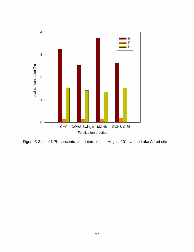
97
Fertilization practice
CMP DOHS-Swingle MOHS DOHS-C-35
Le
af
co
nce
ntr
atio
n (
%)
0
1
2
3
4
N
P
K
Figure 3-3. Leaf NPK concentration determined in August 2011 at the Lake Alfred site

98
Table 3-1. 2M KCl extractable NH4+-N and NO3--N, M1K and M1P concentrations of soil samples collected in June 2009
at SWFREC
Fertigation method NH4+-N NO3
--N M1P M1K
IRR‡ NI IRR NI IRR NI IRR NI
mg kg-1
CMP 1.10 -§ 1.63 - 33.52 - 5.61 -
DOHS 1.65 1.07 2.45 1.69 78.16 31.47 8.06 8.30
MOHS 1.47 1.58 1.78 1.40 25.05 20.67 6.9 5.54
Soil depth (cm)
0-15 1.26 1.10 2.15 2.01 36.81 35.72 6.55 7.66
15-30 1.18 1.03 1.25 1.31 20.24 17.50 5.01 6.45
Statistics¶
Fertigation method *** NS ** ***
Depth * NS ** *
Distance from the tree NS *** *** **
Fertigation method*Depth * NS NS NS
Fertigation method*Distance NS NS NS NS
Depth*Distance NS NS NS NS
Fertigation method*Depth*Distance NS NS NS NS
‡IRR-Irrigated, NI-Non-irrigated, §For conventional practice, all the sampled locations were irrigated. ¶NS-not significant p>0.05; *-p<0.05, **-p<0.01, ***-p<0.001

99
Table 3-2. 2M KCl extractable NH4+-N and NO3--N, M1K and M1P concentrations of soil samples collected in August
2009 at SWFREC
Irrigation method NH4+-N NO3
-N M1P M1K
Soil depth IRR¶ NI IRR NI IRR NI IRR NI
cm mg kg-1
CMP 0-15 1.47 -§ 1.35 - 32.10 - 13.10 -
15-30 1.12 1.20 12.80 11.27
DOHS 0-15 1.54 1.30 1.50 1.22 35.78 24.97 13.45 12.72 15-30 0.74 1.04 1.01 1.38 11.20 22.78 11.11 12.61
MOHS 0-15 2.03 1.81 1.63 1.51 50.62 22.10 13.55 13.19
15-30 1.54 1.61 1.08 1.23 11.98 9.61 11.67 9.06
Statistics‡
Irrigation method NS NS NS
Depth NS ** *** NS
Distance from the tree NS NS * NS Irrigation method*Depth NS NS NS NS
Irrigation method*Distance NS NS NS NS
Depth*Distance NS NS ** NS Irrigation method *Depth*Distance
NS NS NS NS
¶IRR-Irrigated, NI-Non-irrigated, §For conventional practices, all the sampled locations were irrigated. ‡NS-not significant p>0.05; *-p<0.05, **-p<0.01, ***-p<0.001

100
Table 3-3. 2M KCl extractable NH4+-N and NO3
--N, M1K and M1P concentrations of soil samples collected in June 2010 at SWFREC
Fertigation method NH4+-N NO3
--N M1P M1K
Soil depth IRR¶ NI IRR NI IRR NI IRR NI
cm mg kg-1
CMP 0-15 2.07 -§ 6.44 - 48.04 - 14.88 -
15-30 1.75 - 4.70 - 27.93 - 15.53 -
30-45 1.32 - 3.50 - 17.15 - 12.28 -
DOHS 0-15 4.19 3.95 4.34 3.91 81.80 36.73 21.32 15.53
15-30 2.98 2.02 3.23 2.50 32.78 20.41 14.45 9.67
30-45 2.03 1.44 2.60 2.15 15.59 11.44 10.61 7.21
MOHS 0-15 3.33 3.69 5.24 4.70 81.24 30.89 14.21 10.23
15-30 1.89 2.97 3.98 7.40 34.31 28.23 10.61 8.90
30-45 1.57 2.78 2.77 3.37 23.46 14.05 9.45 7.59
Statistics‡
Fertigation method *** *** NS ***
Depth *** *** *** *** Distance from the tree NS NS *** NS
Fertigation method*Depth NS NS NS *
Fertigation method*Distance ** NS * *
Depth*Distance NS NS *** NS
Fertigation method*Depth*Distance NS NS NS NS ¶IRR-Irrigated, NI-Non-irrigated, §For conventional practices, all the sampled locations were irrigated. ‡NS-not significant p>0.05; *-p<0.05, **-p<0.01, ***-p<0.001

101
Table 3-4. 2M KCl extractable NH4+-N and NO3
--N, M1K and M1P concentrations of soil samples collected in December 2009 at the Lake Alfred site
Irrigation method NH4+-N NO3
-N M1P M1K
Soil depth
IRR¶ NI IRR NI IRR NI IRR NI
cm mg kg-1
CMP 0-15 1.40 -§ 4.02 101.29 63.10
15-30 1.03 4.39 91.49 56.28 DOHS-Swingle 0-15 1.18 1.23 1.65 1.74 154.74 104.10 10.70 13.48 15-30 0.92 0.83 1.48 1.43 136.33 122.42 7.06 8.98
DOHS-C35 0-15 1.59 1.75 1.71 1.49 209.24 104.72 31.75 22.90
15-30 1.35 1.10 1.38 1.47 167.92 99.45 29.16 12.57
MOHS 0-15 1.12 1.53 147.01 37.97
15-30 0.94 1.62 139.35 24.58
Statistics‡
Irrigation method * *** *** ***
Depth ** NS NS **
Distance from the tree NS NS *** NS
Irrigation method*Depth NS NS NS NS
Irrigation method*Distance NS ** *** ** Depth*Distance * NS NS NS
Irrigation method *Depth*Distance
NS NS NS NS
¶IRR-Irrigated, NI-Non-irrigated, §For conventional practice and MOHS in December 2009, all the sampled locations were irrigated, ‡NS-not significant p>0.05; *-p<0.05, **-p<0.01, ***-p<0.001

102
Table 3-5. 2M KCl extractable NH4+-N and NO3
--N, M1K and M1P concentrations of soil samples collected in July 2010 at the Lake Alfred site
Irrigation method NH4+-N NO3
-N M1P M1K
Soil depth IRR¶ NI IRR NI IRR NI IRR NI
cm mg kg-1
CMP 0-15 10.49 -§ 20.55 - 105.96 - 46.04 -
15-30 9.51 17.40 98.00 35.00
DOHS-Swingle 0-15 2.64 2.12 7.59 6.31 105.88 88.52 35.56 24.55 15-30 2.98 2.77 3.97 2.71 99.08 93.51 27.29 18.13
DOHS-C35 0-15 0.82 0.59 6.83 5.56 158.31 121.55 26.72 24.29
15-30 0.62 0.60 3.07 2.95 134.61 106.70 17.98 19.97
MOHS 0-15 2.09 1.63 6.64 7.35 114.69 115.87 24.79 25.98
15-30 2.21 1.48 3.55 3.55 126.04 131.63 21.42 21.39
Statistics‡
Irrigation method *** *** *** ***
Depth NS *** NS ***
Distance from the tree NS NS NS NS
Irrigation method*Depth NS NS NS NS
Irrigation method*Distance NS ** NS *
Depth*Distance NS NS NS NS
Irrigation method *Depth*Distance NS NS NS NS ¶IRR-Irrigated, NI-Non-irrigated, §For conventional practices, all the sampled locations were irrigated. ‡NS-not significant p>0.05; *-p<0.05, **-p<0.01, ***-p<0.001

103
Ammonium-N-CMP-June 2009
Cross-row (cm)
0 10 20 30 40
With
in r
ow (
cm)
0
5
10
15
20
25
30
0.7
0.8
0.9
1.0
1.1
1.2
1.3
1.4
Ammonium-N-DOHS-JUNE 2009
Cross-row (cm)
0 10 20 30 40
0
5
10
15
20
25
30
0.8
1.0
1.2
1.4
1.6
1.8
2.0
2.2
Ammonium-N-MOHS-June 2009
0 10 20 30 40
0
5
10
15
20
25
30
1.0
1.2
1.4
1.6
1.8
2.0
2.2
Ammonium-N-CMP-June 2010
Cross-row (cm)
0 10 20 30 40
With
in r
ow (
cm)
0
5
10
15
20
25
30
1.2
1.4
1.6
1.8
2.0
2.2
Ammonium-N-DOHS-June 2010
Cross-row (cm)
0 10 20 30 40
0
5
10
15
20
25
30
1.5
2.0
2.5
3.0
3.5
Ammonium-N-MOHS June 2010
Cross-row (cm)
0 10 20 30 40
0
5
10
15
20
25
30
1.5
2.0
2.5
3.0
3.5
4.0
4.5
5.0
NH4 (mg kg-1)
Cross-row (cm)
Figure 3-4. Lateral ammonium N distribution at 0-30 cm soil depth in June 2009 and 2010 at the Immokalee site

104
Nitrate-N-CMP June 2009
Cross-row (cm)
0 10 20 30 40
With
in r
ow
(cm
)
0
5
10
15
20
25
30
1.2
1.4
1.6
1.8
2.0
2.2
Nitrate-N-DOHS June 2009
Cross-row (cm)
0 10 20 30 40
0
5
10
15
20
25
30
1.4
1.6
1.8
2.0
2.2
2.4
Nitrate-N-MOHS June 2009
Cross-row (cm)
0 10 20 30 40
0
5
10
15
20
25
30
Nitrate-N-CMP June 2010
Cross-row (cm)
0 10 20 30 40
With
in r
ow
(cm
)
0
5
10
15
20
25
30
3.5
4.0
4.5
5.0
5.5
6.0
6.5
Nitrate-DOHS June 2010
Cross-row (cm)
0 10 20 30 40
0
5
10
15
20
25
30
2.2
2.4
2.6
2.8
3.0
3.2
3.4
3.6
Nitrate-N-MOHS June 2010
Cross-row (cm)
0 10 20 30 40
0
5
10
15
20
25
30
3.5
4.0
4.5
5.0
NO3 (mg kg
-1)
0.8 1.0 1.2 1.4 1.6 1.8 2.0 2.2
Figure 3-5. Lateral nitrate N distribution in June 2009 and 2010 at Immokalee site

105
Ammonium-N-CMP
Cross-row (cm)
0 2 4 6 8 10 12 14
With
in r
ow (
cm)
0
2
4
6
8
10
12
14
1.05
1.10
1.15
1.20
1.25
1.30
1.35
1.40
Ammonium-N-MOHS
Cross-row (cm)
0 2 4 6 8 10 12 14
0
2
4
6
8
10
12
14
0.93
0.96
0.98
1.00
1.02
1.04
1.06
1.08
1.10
Ammonium-N-DOHS-Swingle
Cross-row (cm)
0 2 4 6 8 10 12 14
With
in r
ow (
cm)
0
2
4
6
8
10
12
14
1.01
1.02
1.03
1.04
1.05
Ammonium-N-DOHS-C35
Cross-row (cm)
0 2 4 6 8 10 12 14
0
2
4
6
8
10
12
14
1.35
1.40
1.45
1.50
NH4 (mg kg-1)
Figure 3-6. Lateral ammonium N distribution in December 2009 on Candler fine sand

106
Ammonium-N-DOHS-C35
Cross-row (cm)
0 5 10 15 20 25 30
With
in r
ow
(cm
)
0
5
10
15
20
25
30
0.4
0.5
0.6
0.7
0.8
0.9
Ammonium-N-CMP
Cross-row (cm)
0 5 10 15 20 25 30
With
in r
ow
(cm
)
0
5
10
15
20
25
30
4
6
8
10
12
14
16
Ammonium-N-DOHS-SWINGLE
Cross-row (cm)
0 5 10 15 20 25 30
With
in r
ow
(cm
)
0
5
10
15
20
25
30
2.0
2.5
3.0
3.5
4.0
4.5
Ammonium-N-MOHS
Cross-row (cm)
0 5 10 15 20 25 30
With
in r
ow
(cm
)
0
5
10
15
20
25
30
1.5
2.0
2.5
3.0
NH4 (mg kg
-1)
Figure 3-7. Lateral ammonium N distribution in July 2010 at the Lake Alfred site

107
Nitrate-N-CMP
Cross-row (cm)
0 2 4 6 8 10 12 14
With
in r
ow
(cm
)
0
2
4
6
8
10
12
14
2
3
4
5
6
7
8
Nitrate-N-DOHS-35
Cross-row (cm)
0 2 4 6 8 10 12 14
With
in r
ow
(cm
)
0
2
4
6
8
10
12
14
1.40
1.45
1.50
1.55
1.60
1.65
Nitrate-N-DOHS-SWINGLE
Cross-row (cm)
0 2 4 6 8 10 12 14W
ithin
ro
w (
cm)
0
2
4
6
8
10
12
14
1.40
1.45
1.50
1.55
1.60
1.65
1.70
1.75
Nitrate-N-MOHS
Cross-row (cm)
0 2 4 6 8 10 12 14
With
in r
ow
(cm
)
0
2
4
6
8
10
12
14
1.45
1.50
1.55
1.60
1.65
1.70
1.75
1.80
1.85
NO3 (mg kg
-1)
Figure 3-8. Lateral nitrate N distribution in December 2009 at the Lake Alfred site
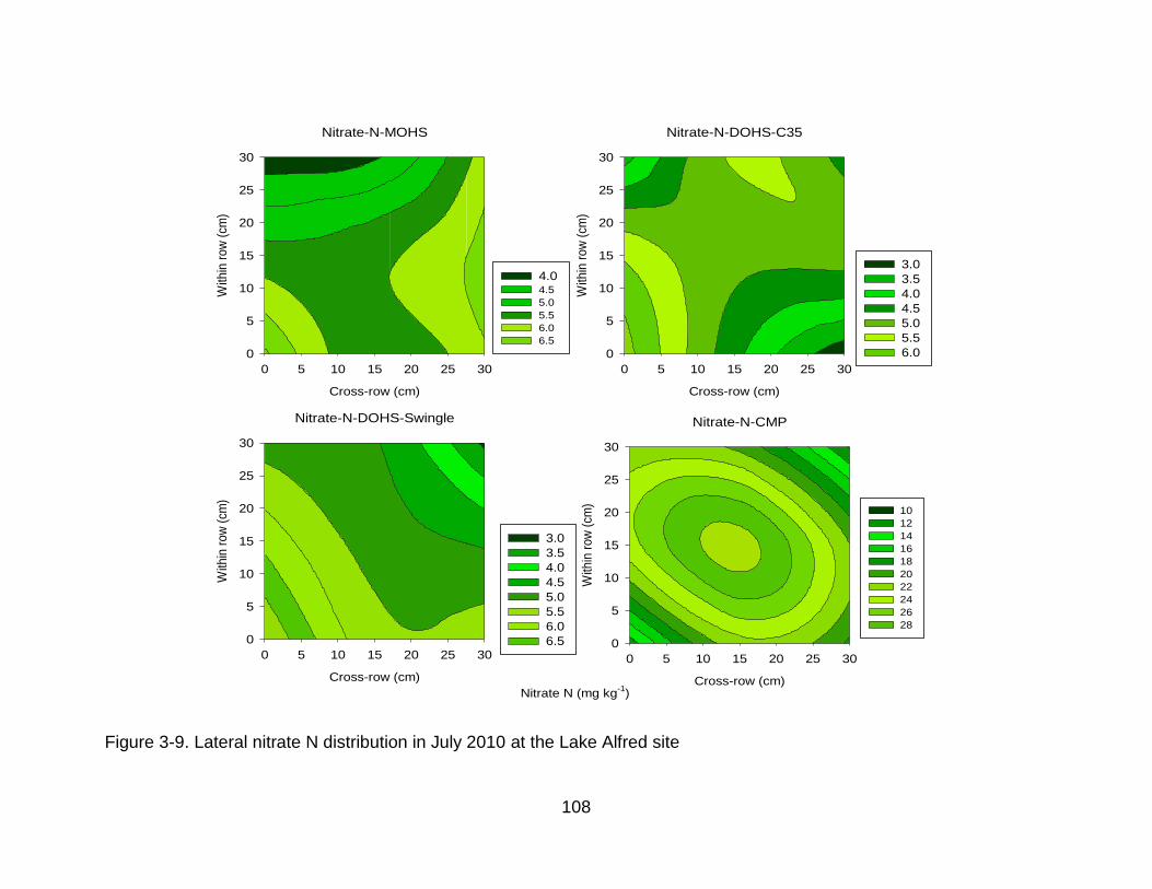
108
Nitrate-N-DOHS-C35
Cross-row (cm)
0 5 10 15 20 25 30
With
in r
ow
(cm
)
0
5
10
15
20
25
30
3.0
3.5
4.0
4.5
5.0
5.5
6.0
Nitrate-N-DOHS-Swingle
Cross-row (cm)
0 5 10 15 20 25 30
With
in r
ow
(cm
)
0
5
10
15
20
25
30
3.0
3.5
4.0
4.5
5.0
5.5
6.0
6.5
Nitrate-N-MOHS
Cross-row (cm)
0 5 10 15 20 25 30
With
in r
ow
(cm
)
0
5
10
15
20
25
30
4.0 4.5
5.0
5.5
6.0
6.5
Nitrate-N-CMP
Cross-row (cm)
0 5 10 15 20 25 30
With
in r
ow
(cm
)
0
5
10
15
20
25
30
10
12
14
16
18
20
22
24
26
28
Nitrate N (mg kg-1
)
Figure 3-9. Lateral nitrate N distribution in July 2010 at the Lake Alfred site
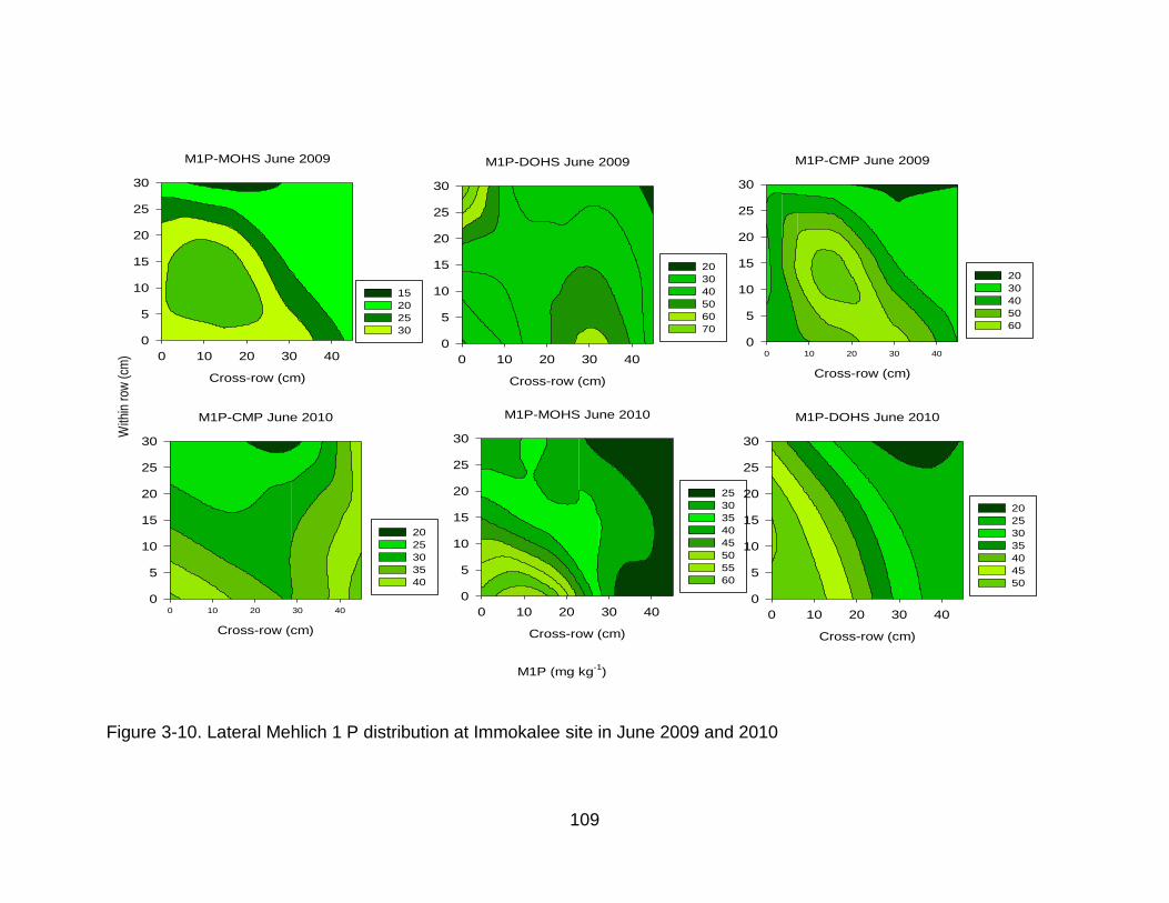
109
M1P (mg kg-1
)
M1P-CMP June 2009
Cross-row (cm)
0 10 20 30 40
0
5
10
15
20
25
30
20
30
40
50
60
M1P-DOHS June 2009
Cross-row (cm)
0 10 20 30 40
0
5
10
15
20
25
30
20
30
40
50
60
70
M1P-MOHS June 2009
Cross-row (cm)
0 10 20 30 40
0
5
10
15
20
25
30
15
20
25
30
M1P-CMP June 2010
Cross-row (cm)
0 10 20 30 40
With
in r
ow (
cm)
0
5
10
15
20
25
30
20
25
30
35
40
M1P-MOHS June 2010
Cross-row (cm)
0 10 20 30 40
0
5
10
15
20
25
30
25
30
35
40
45
50
55
60
M1P-DOHS June 2010
Cross-row (cm)
0 10 20 30 40
0
5
10
15
20
25
30
20
25
30
35
40
45
50
Figure 3-10. Lateral Mehlich 1 P distribution at Immokalee site in June 2009 and 2010

110
M1P-CMP
Cross-row (cm)
0 2 4 6 8 10 12 14
With
in r
ow (
cm)
0
2
4
6
8
10
12
14
94
95
96
97
98
99
100
M1P-MOHS
Cross-row (cm)
0 2 4 6 8 10 12 14
With
in r
ow (
cm)
0
2
4
6
8
10
12
14
130
135
140
145
150
155
160
165
M1P-DOHS-Swingle
Cross-row (cm)
0 2 4 6 8 10 12 14
With
in r
ow (
cm)
0
2
4
6
8
10
12
14
120
130
140
150
160
170
M1P-DOHS-C35
Cross-row (cm)
0 2 4 6 8 10 12 14W
ithin
row
(cm
)0
2
4
6
8
10
12
14
100
120
140
160
180
200
220
M1P (mg kg-1)
Figure 3-11. Lateral Mehlich 1 P distribution in the 0-30 cm depth layer at the Lake Alfred site in December 2009

111
M1P-DOHS-C35
Cross-row (cm)
0 5 10 15 20 25 30
With
in r
ow (
cm)
0
5
10
15
20
25
30
110
120
130
140
150
160
M1P-DOHS-Swingle
Cross-row (cm)
0 5 10 15 20 25 30
With
in r
ow (
cm)
0
5
10
15
20
25
30
75
80
85
90
95
100
105
M1P-MOHS
Cross-row (cm)
0 5 10 15 20 25 30W
ithin
row
(cm
)0
5
10
15
20
25
30
115
120
125
130
135
140
145
M1P-CMP
Cross-row (cm)
0 5 10 15 20 25 30
With
in r
ow (
cm)
0
5
10
15
20
25
30
70
80
90
100
110
120
130
140
Figure 3-12. Lateral Mehlich 1 P distribution in the 0-30 cm depth layer at the Lake Alfred site in July 2010

112
M1K-CMP June 2009
Cross-row (cm)
0 10 20 30 40
0
5
10
15
20
25
30
5.0
5.5
6.0
6.5
7.0
M1K-DOHS June 2009
Cross-row (cm)
0 10 20 30 40
0
5
10
15
20
25
30
6
8
10
12
14
M1K-MOHS June 2009
Cross-row (cm)
0 10 20 30 40
With
in r
ow
(cm
)
0
5
10
15
20
25
30
4
5
6
7
8
9
10
M1K-CMP June 2010
Cross-row (cm)
0 10 20 30 40
0
5
10
15
20
25
30
12
14
16
18
20
M1K-DOHS June 2010
Cross-row (cm)
0 10 20 30 40
0
5
10
15
20
25
30
8
10
12
14
16
18
20
M1K-MOHS June 2010
Cross-row (cm)
0 10 20 30 40
With
in r
ow
(cm
)
0
5
10
15
20
25
30
6
8
10
12
14
M1K (mg kg-1
)
Figure 3-13. Lateral Mehlich 1 K distribution at Immokalee in June 2009 and 2010

113
M1K-CMP
Cross-row (cm)
0 2 4 6 8 10 12 14
With
in r
ow (
cm)
0
2
4
6
8
10
12
14
45
50
55
60
65
M1K-DOHS-Swingle
Cross-row (cm)
0 2 4 6 8 10 12 14
0
2
4
6
8
10
12
14
8.5
9.0
9.5
10.0
10.5
11.0
11.5
12.0
12.5
M1K-MOHS
Cross-row (cm)
0 2 4 6 8 10 12 14
With
in r
ow (
cm)
0
2
4
6
8
10
12
14
26
27
28
29
30
31
32
33
M1K-DOHS-C35
Cross-row (cm)
0 2 4 6 8 10 12 14
0
2
4
6
8
10
12
14
18
20
22
24
26
28
30
M1K (mg kg-1
)
Figure 3-14. Lateral Mehlich 1 K distribution at the Lake Alfred site in December 2009

114
M1K-DOHS-C35
Cross-row (cm)
0 5 10 15 20 25 30
With
in r
ow (
cm)
0
5
10
15
20
25
30
20
21
22
23
24
25
M1K-CMP
Cross-row (cm)
0 5 10 15 20 25 30
With
in r
ow (
cm)
0
5
10
15
20
25
30
30
35
40
45
50
55
60
65
M1K-MOHS
Cross-row (cm)
0 5 10 15 20 25 30
With
in r
ow (
cm)
0
5
10
15
20
25
30
21
22
23
24
25
26
M1K-DOHS-Swingle
Cross-row (cm)
0 5 10 15 20 25 30
With
in r
ow (
cm)
0
5
10
15
20
25
30
18
20
22
24
26
28
30
32
34
M1K (mg kg-1
Figure 3-15. Lateral Mehlich 1 K distribution at the Lake Alfred site in July 2010

115
Ammonium N (mg kg-1)
0.0 0.5 1.0 1.5 2.0 2.5 3.0 3.5
De
pth
(cm
)
0
20
40
60
80
100
120
140
CMP
DOHS
MOHS
Nitrate N (mg kg-1)
0 2 4 6 8 10
De
pth
(cm
)0
20
40
60
80
100
120
140
CMP
DOHS
MOHS
Ammonium N (mg kg-1)
0 2 4 6 8 10
De
pth
(cm
)
0
20
40
60
80
100
120
140
DOHS-Swingle
CMP
DOHS-C35
MOHS
Nitrate N (mg kg-1)
0 5 10 15 20 25
De
pth
(cm
)
0
20
40
60
80
100
120
140
DOHS-Swingle
CMP
DOHS-C35
MOHSA
B
C
D
Figure 3-16. Vertical nitrate N and ammonium N distribution in June 2010 at Immokalee
site (A and B) and in July 2010 at the Lake Alfred site (C and D)

116
Mehlich 1 P (mg kg-1)
20 40 60 80 100 120 140 160
Depth
(cm
)
0
20
40
60
80
100
120
140
DOHS-Swingle
CMP
DOHS-C35
MOHS
Mehlich 1 P (mg kg-1)
0 10 20 30 40 50
Depth
(cm
)0
20
40
60
80
100
120
140
DOHS
CMP
MOHS
Figure 3-17. Vertical M1P distribution in June 2010 at Immokalee site (A) and in July 2010 at the Lake Alfred site (B)
Mehlich 1 K (mg kg-1)
15 20 25 30 35 40 45
Depth
(cm
)
0
20
40
60
80
100
120
140
DOHS-Swingle
CMP
DOHS-C35
MOHS
Mehlich 1 K (mg kg-1)
4 6 8 10 12 14 16 18
Depth
(cm
)
0
20
40
60
80
100
120
140
CMP
DOHS
MOHS
A B
Figure 3-18. Vertical M1K distribution in June 2010 at Immokalee site (A) and in July 2010 at the Lake Alfred site (B)

117
Table 3-6. Fresh and dry tissue weight for samples collected in July 2011 at Immokalee
Fertigation method CMP DOHS MOHS
Tissue FW¶ % DW % FW % DW % FW % DW %
Young leaves 4,391.4 12.8 1,598.2 10.3 2,989.9 8.3 1,017.4 6.7 3,349.0 9.2 1,208.0 8.0
Fully expanded leaves 923.5 2.7 340.9 2.2 5,712.3 15.8 1,947.1 12.8 3,350.9 9.2 1,212.3 8.0
Fruits 12,922.7 37.5 3,657.3 23.5 9,685.8 26.8 1,763.8 11.6 13,557.9 37.2 3,111.9 20.6
Twigs 2,890.0 8.4 1,480.0 9.5 3,394.6 9.4 1,700.0 11.2 3,589.9 9.9 1,800.0 11.9
Small branches 1,187.6 3.5 676.0 4.4 1,186.5 3.3 650.3 4.3 1,124.3 3.1 667.5 4.4
Medium branches 1,065.9 3.1 633.4 4.1 1,474.2 4.1 847.0 5.6 952.5 2.6 542.2 3.6
Large branches 2,156.1 6.3 1,286.2 8.3 1,134.0 3.1 655.7 4.3 1,678.3 4.6 1,006.5 6.7
Trunk 3,447.3 10.0 2,143.9 13.8 3,243.2 9.0 1,934.2 12.8 3,164.4 8.7 1,869.5 12.4
Total above-ground 28,984.5 84.2 11,815.7 76.0 28,820.4 79.7 10,515.5 69.4 30,767.3 84.5 11,418.0 75.4
Roots (<0.5mm) 501.0 1.5 253.6 1.6 298.4 0.8 155.7 1.0 653.0 1.8 329.0 2.2
Roots (0.5-1mm) 84.9 0.3 67.3 0.4 449.2 1.2 273.5 1.8 100.9 0.3 86.0 0.6
Roots (1-3mm) 335.0 1.0 252.9 1.6 1,155.5 3.2 547.1 3.6 383.6 1.1 322.0 2.1
Roots (>3mm) 4,532.8 13.2 3,153.7 20.3 5,432.0 15.0 3,667.5 24.2 4,525.3 12.4 2,979.9 19.7
Total below-ground 5,453.7 15.8 3,727.5 24.0 7,335.1 20.3 4,643.8 30.6 5,662.9 15.5 3,716.9 24.6
Total 34,438.2 100.0 15,543.2 100.0 36,155.5 100.0 15,159.3 100.0 36,430.1 100.0 15,134.9 100.0 ¶FW-Fresh weight, DW-Dry weight in g

118
Table 3-7. Fresh and dry tissue weight for samples collected in August 2011 at the Lake Alfred site
Irrigation method
CMP DOHS-Swingle MOHS DOHS-C35
Tissue ¶FW % DW % FW % DW % FW % DW % FW % DW % Leaves
160.1
12.6
60.2
26.5
199.7
15.8
72.1
31.7
163.4
12.9
56.7
25.0
166.0
13.1
59.3
26.1
Fruits
811.5
64.1
104.7
46.1
1,003.8
79.3
123.8
54.5
850.6
67.2
104.4
45.9
844.4
66.7
103.7
45.6
Twigs
24.6
1.9
10.5
4.6
43.1
3.4
19.8
8.7
32.9
2.6
14.2
6.2
32.8
2.6
14.3
6.3
Total above-ground
996.1
97.1
175.5
90.8
1,246.6
98.4
215.7
94.9
1,046.9
96.0
175.3
94.7
1,043.2
97.8
177.3
91.7
Small roots (<0.5 mm)
4.0
0.3
2.8
1.2
6.1
0.5
4.7
2.1
5.4
0.4
4.5
2.0
4.5
0.4
3.1
1.4
Medium roots (0.5-1 mm)
1.2
0.1
0.6
0.3
1.3
0.1
0.3
0.1
1.3
0.1
0.9
0.4
0.9
0.1
2.0
0.9
Large roots (1-3 mm)
5.0
0.4
2.6
1.1
6.3
0.5
2.9
1.3
4.4
0.3
3.0
1.3
3.1
0.2
1.5
0.7
Largest root (>3 mm)
20.0
1.6
11.8
5.2
6.2
0.5
3.7
1.6
32.5
2.6
1.5
0.7
14.8
1.2
9.4
4.1
Total below-ground
30.1
2.9
17.8
9.2
20.0
1.6
11.6
5.1
43.6
4.0
9.9
5.3
23.2
2.2
16.0
8.3
Total
1,026.3
100.0
193.3
100.0
1,266.6
100.0
227.3
100.0
1,090.5
100.0
185.2
100.0
1,066.5
100.0
193.3
100.0
¶FW-Fresh weight, DW-Dry weight in g

119
Table 3-8. N, P and K concentration in tissues collected in July 2011 at the Immokalee site
Fertigation method CMP DOHS MOHS
Tissue N P K N P K N P K
%
Young leaves 2.58 0.14 1.83 3.25 0.11 1.11 3.33 0.12 1.36
Old, fully expanded leaves 2.31 0.15 1.35 3.53 0.12 1.20 2.94 0.13 1.17
Twigs 1.22 0.13 1.45 1.54 0.14 1.15 1.30 0.17 1.36
Small branches 0.37 0.13 0.88 0.58 0.11 1.13 0.86 0.13 0.89
Medium branches 0.34 0.14 1.29 0.71 0.11 0.92 0.32 0.13 1.12
Large branches 0.53 0.17 1.30 0.45 0.16 1.41 0.54 0.12 1.22
Trunk 0.60 0.18 1.35 0.99 0.14 1.36 0.95 0.15 1.15
Fruits 1.25 0.15 1.41 1.83 0.12 1.55 1.97 0.15 1.26 Small roots (<0.5 mm) 1.38 0.14 1.19 2.26 0.11 1.12 1.91 0.13 1.31
Medium roots (0.5-1 mm) 1.21 0.13 1.21 1.60 0.13 1.15 1.46 0.13 1.37
Large roots (1-3 mm) 0.65 0.14 1.19 1.11 0.15 1.55 2.62 0.14 1.43
Largest root (>3 mm) 0.56 0.16 1.27 0.78 0.13 1.41 0.85 0.17 1.42
Table 3-9. N, P and K concentration in tissues collected in August 2011 at the Lake Alfred site
Irrigation method CMP DOHS-Swingle MOHS DOHS-C35
Tissue N P K N P K N P K N P K
%
Leaves 3.25 0.13 1.53 2.52 0.13 1.41 3.73 0.14 1.33 2.62 0.20 1.52
Fruits 1.27 0.11 0.93 1.05 0.12 1.01 1.69 0.13 1.33 2.42 0.19 1.47
Twigs 1.26 0.11 1.13 1.06 0.16 1.41 1.36 0.14 1.09 1.07 0.15 1.32
Small roots (<0.5 mm) 2.14 0.18 1.25 2.05 0.15 1.28 1.70 0.13 1.43 2.21 0.18 0.45
Medium roots (0.5-1 mm) 1.78 0.17 1.20 2.09 0.23 2.28 0.99 0.26 2.21 0.58 0.17 0.75
Large roots (1-3 mm) 1.26 0.12 1.09 1.26 0.13 1.24 0.85 0.14 1.47 0.86 0.11 0.33
Largest root (>3 mm) 1.11 0.12 1.01 0.89 0.14 1.53 1.70 0.16 1.49 0.99 0.11 0.33

120
Table 3-10. Nitrogen, phosphorus and potassium accumulation on Immokalee sand
Fertigation method CMP DOHS MOHS CMP DOHS MOHS CMP DOHS MOHS
Tissue N P K
kg ha-1
Young leaves 20.16 16.17 19.67 1.09 0.55 0.71 14.30 5.52 8.03
Old, fully expanded leaves 3.85 33.61 17.43 0.25 1.14 0.77 2.25 11.43 6.94
Fruits 22.36 15.78 29.98 2.68 1.03 2.28 25.22 13.37 19.17
Twigs 8.83 12.80 11.44 0.94 1.16 1.50 10.49 9.56 11.97
Small branches 1.22 1.84 2.81 0.43 0.35 0.42 2.91 3.59 2.91
Medium branches 1.05 2.94 0.85 0.43 0.46 0.34 4.00 3.81 2.97
Large branches 3.33 1.44 2.66 1.07 0.51 0.59 8.18 4.52 6.00
Trunk 6.29 9.36 8.68 1.89 1.32 1.37 14.15 12.86 10.51
Small roots (<0.5 mm) 1.71 1.72 3.07 0.17 0.08 0.21 1.48 0.85 2.11
Medium roots (0.5-1 mm) 0.40 2.14 0.61 0.04 0.17 0.05 0.40 1.54 0.58
Large roots (1-3 mm) 0.80 2.97 4.13 0.17 0.40 0.22 1.47 4.15 2.25
Largest root (>3 mm) 8.64 13.99 12.39 2.47 2.33 2.48 19.59 25.29 20.69 †Total 78.65 114.78 113.72 11.64 9.52 10.95 104.43 96.49 94.13
†Total NPK accumulation is fairly low compared with accumulation observed in a typical orange grove owing to citrus
greening infection

121
Table 3-11. N, P and K accumulation in 2011 at the Lake Alfred and Immokalee sites
Irrigation method CMP DOHS-Swingle MOHS DOHS-C35
Lake Alfred N P K N P K N P K N P K
g kg-1
Leaves 32.5 1.3 15.3 25.2 1.3 14.1 37.3 1.4 13.3 26.2 2.0 15.2
Fruits 12.7 1.1 9.3 10.5 1.2 10.1 16.9 1.3 13.3 24.2 1.9 14.7
Twigs 12.6 1.1 11.3 10.6 1.6 14.1 13.6 1.4 10.9 10.7 1.5 13.2
Small roots (<0.5 mm) 21.4 1.8 12.5 20.5 1.5 12.8 17.0 1.3 14.3 22.1 1.8 4.5
Medium roots (0.5-1 mm) 17.8 1.7 12.0 20.9 2.3 22.8 9.9 2.6 22.1 5.8 1.7 7.5
Large roots (1-3 mm) 12.6 1.2 10.9 12.6 1.3 12.4 8.5 1.4 14.7 8.6 1.1 3.3
Largest root (>3 mm) 11.1 1.2 10.1 8.9 1.4 15.3 17.0 1.6 14.9 9.9 1.1 3.3
Fertigation method CMP DOHS MOHS
Immokalee N P K N P K N P K
Young leaves 25.8 1.4 18.3 32.5 1.1 11.1 33.3 1.2 13.6
Fully expanded leaves 23.1 1.5 13.5 35.3 1.2 12.0 29.4 1.3 11.7
Fruits 12.2 1.3 14.5 15.4 1.4 11.5 13.0 1.7 13.6
Twigs 3.7 1.3 8.8 5.8 1.1 11.3 8.6 1.3 8.9
Small branches 3.4 1.4 12.9 7.1 1.1 9.2 3.2 1.3 11.2
Medium branches 5.3 1.7 13.0 4.5 1.6 14.1 5.4 1.2 12.2
Large branches 6.0 1.8 13.5 9.9 1.4 13.6 9.5 1.5 11.5
Trunk 12.5 1.5 14.1 18.3 1.2 15.5 19.7 1.5 12.6
Roots (<0.5mm) 13.8 1.4 11.9 22.6 1.1 11.2 19.1 1.3 13.1
Roots (0.5-1mm) 12.1 1.3 12.1 16.0 1.3 11.5 14.6 1.3 13.7
Roots (1-3mm) 6.5 1.4 11.9 11.1 1.5 15.5 26.2 1.4 14.3
Roots (>3mm) 5.6 1.6 12.7 7.8 1.3 14.1 8.5 1.7 14.2

122
CHAPTER 4 EFFECTS OF FERTIGATION AND IRRIGATION RATES ON ROOT LENGTH
DISTRIBUTION AND TREE SIZE
The use of automated irrigation systems and intensive nutrient management is
critical to citrus production systems for achieving increased tree growth and yield.
Maintenance of soil moisture and nutrient concentrations in the tree root zone near
optimum levels is known as the open hydroponic system (OHS) (Morgan et al., 2009b).
Sound water and nutrient management is required in Florida soils with high sand
content (>94%) and low organic matter content because leaching and subsequent
pollution of groundwater is a likely threat.
Key to improving citrus nutrient and water uptake is the understanding of the root
system dimensions, topological properties and distribution in the soil. Of these root
properties, the property of greatest importance is root length density (RLD) distribution
because it defines limits to the efficiency of a root system in absorbing water and
nutrients (Tinker and Nye, 2000; Himmelbauer et al., 2004). Studies on tree RLD
distribution done in Florida by Morgan et al. (2007) found that fibrous root length density
(FRLD) distribution increased with soil depth and lateral distance as trees grew,
resulting in mature trees with bimodal root systems. In their study, they classified
fibrous roots as those roots whose diameter fell between 0-4 mm because such roots
determine tree water and nutrient uptake efficiency. Morgan et al. (2007) reported that
FRLD varied as a function of rootstock in which trees on Swingle citrumelo developed
higher FRLD near the soil surface and lower FRLD below 0.3 m than trees on Carrizo
citrange. Abrisqueta et al. (2008) studied root dynamics of young peach subjected to
partial root zone drying and continuous deficit irrigation in Spain. In the study, higher

123
root length densities were recorded in non-limiting irrigation conditions than under deficit
irrigation where root growth was reduced.
Two methods (plant based or soil based) have been used to estimate and
describe root systems. The plant-based method describes the way in which different
parts of the root system are interconnected (Rose, 1983; Klepper, 1992). The second
method describes root systems in the soil in terms of the distribution of RLD or mass
throughout the rooting zone and has been used as a standard way of measuring density
in distributions of roots in field soils (Barraclough and Leigh, 1984; Vincent and Gregory,
1989a, b; Masse et al., 1991). Basing on the latter, researchers devised methods of soil
coring and root washing to provide the most practicable way of obtaining quantitative
data on root system length and distribution in the field (Tinker and Nye, 2000). The
main methods that have been used for measuring root length over the years are line
intersect method (Newman, 1966); direct measurement and opisometer methods
(Reicosky et al., 1970); photocopying and scanning (Collins et al., 1987; Kirchoff, 1992;
Himmelbauer et al., 2004) and the stereological procedure (Wulfsohn et al., 2004).
Despite its merits, the line intersect method uses a tedious operational procedure which
includes insuring uniform root dispersal throughout a finite area and the repetitive use of
short line intercepts (Reicosky et al., 1970). The study by Reicosky et al. (1970) showed
significant gains in time by using the line intersection method over the direct and
opisometer methods. Reicosky and colleagues found that there was little difference in
precision between the line intersect, direct and opisometer methods for estimating root
length but found more gains on time in using the first method (1.0 h) compared with the
latter two where it took 5.0 h and 1.5 h for the direct and opisometer methods,

124
respectively. Thus, through root scanning, the line intersect method can be calibrated
and used to predict root length with speed and greater precision (Collins et al., 1987;
Bland and Mesarch, 1990).
Studies done in central and south Florida showed that tree size was a function of
root density (Castle and Krezdon, 1975; Ford, 1954; 1964; 1972), root stock (Morgan et
al., 2006a) and fertilization practice (Obreza and Rouse, 1991; 1993; 2006; Morgan et
al., 2009a). Marler and Davies (1990) showed that canopy volume, trunk cross-
sectional area and root dry weight can be influenced by irrigation rate. In their study,
canopy volume and trunk cross-sectional area were similar at high (20 % of available
soil water depletion) and moderate (45 % of available soil water depletion) levels in 2 of
3 years, but were reduced at low (65 % of available soil water depletion). More than 90
% of the roots were within 80 cm of the tree trunk at the end of the growing season.
Parsons et al. (2001), in their study on the effect reclaimed water on citrus tree growth,
found that tree growth was greatest at high irrigation rate (2500 mm) though fruit
production per canopy volume was low compared with lower rates ~400 mm and 1250
mm. However, very little research, if any, has been conducted to determine the effect of
irrigation rate and fertilization method on tree size in Florida using the modified
ACPS/OHS practices. Documentation of the performance of ACPS/OHS practices with
regard to tree size and root density is critical for their adaptation to Florida soil and
climatic conditions.
The objectives of the experiment were to:
(1) calibrate line intersect method for determining RLD in 1- and 3-year old citrus using the digital scanning method on Florida Entisol and Spodosol,

125
2) to determine the effect of fertigation frequency and irrigation method on RLD distribution,
(3) validate the RLD estimated based on root area using the intercept method,
(4) determine root distribution patterns in the irrigated and non-irrigated zones as a function of fertigation method and depth, and,
(5) determine the effect of fertigation frequency and irrigation method on canopy volume and trunk cross-sectional area.
The following hypotheses were postulated:
(1) root area using a flatbed scanner can be calibrated using the line intersect method and used to predict root length with speed and greater precision,
2) spatial root length density distribution will be greater in irrigated zones of microsprinkler and drip OHS than conventional practice, and,
3) microsprinkler and drip OHS will increase citrus growth rate resulting in canopy volumes and trunk cross-sectional areas higher than conventional practice.
Materials and Methods
Description of Study Sites and Treatments
Treatments and orchard locations for this study were the same as trees used in
the nutrient distribution and accumulation study presented in Chapter 3. At the
SWFREC site treatments were: (1) Conventional practice –irrigated weekly and
fertigated monthly (CMP); (2) Drip OHS – irrigated daily and fertigated weekly in small
pulses (DOHS); (3) Microsprinkler OHS – irrigated daily and fertigated weekly (MOHS).
All the treatments were laid in a randomized complete block design replicated four
times. The Hamlin oranges (Citrus sinensis) on Swingle rootstock were planted on a
3.05 x 6.71 m tree and row spacing. A second study was installed at a 15-acre Ridge
site near the Citrus Research and Education Center (CREC), Lake Alfred, with Hamlin
oranges on Swingle rootstocks at 3.05 x 6.10m (~218 trees/acre) and C35 rootstock at
2.44 x 5.49m (~302 trees/acre). The treatments imposed at the Lake Alfred site were

126
similar to the set-up at SWFREC except for the modification to the conventional practice
where the use of dry granular fertilizer applied under the canopy four times a year acted
as a control for the experiment and also DOHS was imposed on both Swingle and C-35
rootstock.
Root Sampling Methods
Roots were sampled for RLD and average root diameter estimations of 3-year old
citrus at SWFREC, on June 9 through 17, 2009 in the 0-30 cm depth at 15 cm depth
increments because this is where most roots of young citrus trees (<3 years old) are
concentrated (Fares and Alva, 2000; Paramasivam et al., 2000c; Parsons and Morgan,
2004). The samples were collected at 0, 15, 30, and 45 cm distance from the tree in the
row in 15 cm increments up to 45 cm from the tree perpendicular to the planted row,
giving a total of 12 sampling locations in one quadrant for each tree (3 x 4 grid). On
June 16 through 24, 2010 root samples at SWFREC were collected up to 45 cm depth
using the above sampling scheme. At the Lake Alfred site, fewer samples than those at
SWFREC were collected using a 2 x 2 grid on December 22, 2009 and a 3 x 3 grid on
July 7 and 8, 2010 at 0-15 cm and 15-30 cm depth.
All the cores were carefully bagged, labeled and stored in a refrigerator at <4 C
awaiting subsequent analysis. Roots were removed from the soil using a 2 mm
diameter sieve. Other debris passing through the sieve was removed manually. The
roots were hydrated for 15 minutes and categorized into four groups according to
diameter: <0.5 mm, 0.5-1.0 mm, 1-3 mm and >3 mm before using the line intersection
method (adapted from Morgan, 2004). Root length for each root category was
estimated using the grid system explained by Tennant (1975) by counting the number of
horizontal and vertical intersections of roots in a grid system of 1.0 x 1.0 cm which was

127
multiplied by 11/14 and divided by volume of the corer to give root length density in cm
cm-3 soil (Mattos, 2000).
Estimation of Tree Growth Characteristics
Tree canopy volumes were made by measuring the average canopy diameter
using canopy width in the east-west and north-south directions and canopy height.
Then, using the formula for a sphere=
r3, where r is the canopy radius (where the
canopy width in the east-west and north-south directions and canopy height were
averaged to give the canopy radius), canopy volume was calculated. Trunk diameter
was estimated from averaging the diameter in the east-west and north-south directions
and then calculating the area using the formula r2, assuming circular shape, where r is
the trunk radius.
Statistical Analysis
Roots of selected root diameters from samples collected in two of the four
replications at SWFREC were designated the calibration set and roots from the
remaining two replications were designated the validation set. The RLD estimate using
the intercept method (dependent variable) and mean root area using the scanning
method (independent variable) for calibration set roots were correlated resulting in a
calibration curve for the root scanning method. To validate the calibration curve,
estimated RLD calculated using the mean root areas of the validation set roots were
correlated with the RLD estimate of the same roots using the intercept method. After
validating the procedure at Immokalee and getting reasonably good calibration curves,
a calibration curve was also determined for estimating RLD at Lake Alfred using similar
calibration and validation techniques. All correlations were done using SAS 9.2

128
PROCREG procedures (SAS Inst. 2011) and SIGMA PLOT 10.0. The rest of the data
were analyzed using PROC GLM Mixed Model Procedures (SAS Inst. 2011) to
determine the effect of the irrigation method and fertilization frequency on vertical and
lateral root length density distribution, and tree growth.
Results and Discussion
Correlation of RLD Measured by Intersection Method versus Scanning Method
Root length density measured using the modified Newman method (Tennant,
1975) correlated well with scanned area of the calibration set at both SWFREC and
Lake Alfred sites (Appendix F). RLDs predicted by the calibration scanning method also
agreed with measured RLDs for the validation set at both SWFREC and the Lake Alfred
site (Tables 4-1 and 4-2). The strong positive correlation for all diameters of roots
collected at both locations shows the precision of using the scanning method upon
calibration with the line intersection method. Only 1.61% of the scanned roots at CREC
and 2.25% of the scanned roots at SWFREC were above the normal deviations (relative
standard deviation 10%) showing that scanning roots in triplicate represent a fairly
accurate and precise way of determining RLD. The equations for the calibration set
using scanned root area provided PLD with reasonable agreement to RLD measured
using the intercept method (greater than R2>0.79) at both study sites. There was close
agreement in the validation set between RLD estimated using the intercept method and
that predicted using the calibration equation developed from root scanning (R2 ranged
from 0.88 to 1.00 at CREC and 0.87 to 0.97 at SWFREC). Lowest coefficient of
determination for roots greater than 3 mm in diameter was noted at CREC owing to few
roots in this root category ascribed to the young tree age. Examination of equation
slopes revealed that of the validation models developed for both sites, only the models

129
for root sizes <0.5. 0.5-1.0, and 1.0-3.0 mm yielded close approximations of predicted
RLD with slopes >0.78 thus nearly a 1:1 ratio, adequately explaining the variability in the
validation and versus calibration sets. Slopes for root sizes >3 mm explained about 50
to 60% of the variability probably because there were very few roots >3 mm at both
sites. The scanning method reduces the time required to measure RLD in samples. In
this study for example, it took about 40 to 60 hours to scan root samples compared with
the line intercept method that took 140 hours (about 10 hours per day, though not
statistically done across different sets of individuals). Considering the importance of
accurate root length estimation, the scanning method offers a worthwhile alternative
especially when the researcher has a large number of samples. Several researchers
approve photocopying (Collins et al., 1987; Kirchoff, 1992) and scanning (Collins et al.,
1987; Bland and Mesarch, 1990) in RLD determination to achieve as much accuracy in
the shortest time possible.
RLD Distribution as a Function of Irrigation Method, Time and Soil Depth
Root samples collected at SWFREC in June 2009 showed that lateral RLD
distribution for CMP decreased from 0.374 cm cm-3 near the tree to 0.084 at 45 cm
away from the tree row (Table 4-3 and Appendix A, Figure A22). The irrigated zones of
DOHS and MOHS showed RLD as high as 0.386 cm cm-3 and 0.279 cm cm-3 that
decreased to 0.139 and 0.053 in the non-irrigated zone respectively (Table 4-1,
Appendix A, Figures A23 and A24). Small roots (<0.5 mm and 0.5-1.0mm in diameter)
accounted for ≥80% of the RLD at both 0-15- and 15-30 cm depths while largest roots
(>3 mm) contributed <3% of the total RLD.
For RLD samples collected at SWFREC in June 2010, fibrous roots (roots <0.5
mm and 0.5-1.0mm in diameter) contributed >77% of RLD while largest roots (>3 mm)

130
accounted for <2 % of total RLD (Table 4-4). For CMP, 49% of the roots were found in
the 0-15 cm depth while 36% and 15% of the roots were observed in the 15-30 cm and
30-45 cm soil depth. About 54%, 35% and 10% were found in the 0-15-, 15-30- and 30-
45 cm depth using DOHS (Table-4-4). Most of the roots (60%) were found in the 0-15
cm depth using MOHS while 23% and 17% of the roots were distributed in the 15-30
and 30-45 cm depth (Table 4-4). Roots (<0.5 mm in diameter) for CMP were uniformly
distributed in the irrigated zones averaging about 0.089 cm cm-3 while the roots greater
0.5 mm in diameter were largely found in the irrigated zone at 15 to 30 cm from the tree.
The lateral root distribution (0.5 mm) for DOHS averaged 0.33 cm cm-3 in the irrigated
and non-irrigated zones of 0-15 cm soil depth layer (Table 4-4) probably because
drippers were increased from 4 to 8 drippers per tree and due to the rainy season
which supplied water even in the nonirrigated zone. However, at 15-30 cm and 30-45
cm soil depths, RLD for (root <0.5 mm in diameter) was approximately 2 times that
observed in the non-irrigated zone while for roots greater than 0.5 mm in diameter the
RLD was similar between the irrigated and non-irrigated zones (Table 4-4). Root
density estimated for MOHS for roots (<0.5 mm in diameter) was two times higher in
irrigated than nonirrigated zone at all depths (Table 4-4) decreasing from 0.33 cm cm-3
in the irrigated zone to about 0.022 cm cm-3 in the nonirrigated zone. In June 2010 at
SWFREC, roots were uniformly distributed laterally in the grid around the tree using
CMP with RLD ranging from 0.154 cm cm-3 to 0.086 cm cm-3 (Figure A25). Root length
density using DOHS decreased from 0.439 cm cm-3 below the dripper to 0.170 cm cm-3
at 45 cm from the tree (Figure A26). Similar pattern for MOHS was noted (Figure A27).
The root densities under the drip at SWFREC were lower than Lake Alfred because the

131
drippers were moved from near the tree trunk to 30 cm away from the tree, when the
number of lines was increased from one to two in March 2010 prior to the June
sampling.
In December 2009, at the Lake Alfred site, RLD was high in irrigated zones of
DOHS-Swingle and DOHS-C35. For example, positions below the dripper showed RLD
of about 0.8 cm cm-3 (DOHS-Swingle) (Appendix A, Figure A28) and 0.86 cm cm-3
(DOHS-C35) (Appendix A, Figure A29) which, respectively, decreased to 0.41 cm cm-3
and 0.091 cm cm-3 with distance away from the tree. The microsprinkler irrigation
methods, CMP (Appendix A, Figure A30) and MOHS (Appendix A, Figure A31), yielded
similar RLD≈0.42 cm cm-3 closer to the tree that decreased laterally to 0.074 cm cm-3
and 0.27 cm cm-3, respectively (Table 4-5). All irrigation methods but CMP showed that
>60% of the roots were concentrated in top 0-15 cm than the 15-30 cm soil depth.
However, CMP showed that 65% of the roots dominated the 15-30 cm soil depth. All
treatments showed that fibrous roots (<0.5 mm and 0.5-1 mm) contributed to > 80% of
the total RLD at both 0-15- and 15-30 cm soil depth suggesting that it is likely that
young trees will develop small, fine roots to promote water and nutrient uptake and
accelerate tree growth. Largest roots (>3 mm) contributed <1.1% of total RLD. These
results are similar to those reported by Morgan et al. (2007) on 2 to 5-year-old Hamlin
and Valencia orange trees. In agreement with our findings, they also reported that citrus
trees develop a dense root system within the upper 30 cm where fibrous RLD
distribution increases with depth and lateral distance as trees grow.
Results suggest that the further away from the tree, the less likely we are to find
roots as shown in the significant decrease in RLD with distance from the tree. Thus,

132
irrigation methods such as drip which apply water and fertilizer frequently and in small
pulses within a limited root zone offer a viable option for increasing root water and
nutrient uptake compared with the microsprinkler based systems when the trees are
small. Positions below drippers tended to have high root density as exemplified in the
DOHS-C35 and DOHS-Swingle where RLD ~0.8 cm cm-3 was close to 2 times that
obtained in the irrigated zones of CMP or MOHS at the Lake Alfred site. Thus, this
should typify the potential for increasing root density and subsequent tree uptake using
drip irrigation.
In July 2010, lateral root distribution showed that RLD decreased gradually with
distance from the tree at the Lake Alfred site. For CMP and MOHS, RLD near the tree
was about 0.25 cm cm-3 and 0.45 cm cm-3 and decreased to 0.10 cm cm-3 and 0.19 cm
cm-3, respectively at 30 cm from the tree (Appendix A, Figures A32 and A35, Table 4-6).
The drip fertigated treatments showed high RLD of about 1.0 cm cm-3 in the irrigated
zone that decreased to 0.20 cm cm-3 in the non-irrigated zone (Appendix A, Figures A33
and A34). Also, the high RLD in the non-irrigated zones for the OHS-based fertigation
methods was not expected. We ascribe the presence of roots in the non-irrigated zone
to the high rainfall in Florida (approximately 1400 mm) which probably increased the
amount of available water including in the non-irrigated zone thus promoting root growth
and development. Obreza and Pitts (2002) also observed similar phenomena on root
density distribution between the irrigated and non-irrigated zones of southwest Florida.
The results show RLD <1.3 cm cm-3, consistent with findings of other researchers in
citrus (Mattos et al., 2003), apple (De Silva et al., 1999) and somewhat lower than the
RLD reported by Coleman (2007) in other woody species. Positions below the dripper or

133
in irrigated zones, except for CMP (probably due to infrequent irrigation), had very high
root length density. Zhang et al. (1996 and1998) also reported that RLD of fibrous roots
was significantly greater near the emitter and at 0-15 cm deep layer for grapefruit trees.
Similar results were obtained in citrus (Alva and Syvertsen, 1991; Mattos et al., 2003a;
Morgan et al., 2007) and in drip-irrigated woody species Coleman (2007). At the Lake
Alfred site, small roots (<0.5 mm) accounted for >87% of the total RLD at 0-15 cm soil
depth using all irrigation methods and >64% at 15-30 cm depth while largest roots
accounted for the smallest portion (<2%) of the total RLD. All other treatments but
grower practice showed high RLD in the top 0-15 cm where 58%, 67% and 57% of the
roots were concentrated using DOHS-Swingle, DOHS-C35 and MOHS, respectively.
Only 36% of the roots were found in the 0-15 cm using the grower practice. Nappi et al.
(1985) and Bassoi et al. (2003) found that highest grapevine root presence was within
the top 40 cm and within 40 cm radius from the trunk for drip and at 0.8-1 m distance
from the trunk using microsprinkler irrigation. In their studies, roots with diameter <2 mm
corresponded to at least 80% of total root length. Overall, root length density found in
this study was higher for drip- than microsprinkler-irrigated citrus, which is similar in
relation to results from Australia (Stevens and Douglas, 1994) and Brazil (Bassoi et al.,
2003). The maximum RLD values reported by Stevens and Douglas (1994) were 1.2
and 0.6 cm cm-3 for drip- and microsprinkler-irrigated 8-yr-old vines, respectively. Thus,
our values, particularly, on the Ridge site are somewhat greater for the tree age (<3 yr-
old) and point to the intensive irrigation and fertigation rates. The study of Stevens and
Douglas (1994) also revealed that 47% and 40% of the roots were found in the top 0-40

134
cm in a 0-160 cm profile of microject and drip irrigation. These observations confirm our
postulated hypothesis that RLD would be greater using OHS-based fertigation methods.
Effect of Fertigation Method on Trunk Cross-Sectional Area and Canopy Volume
DOHS treatments using Swingle and C35 rootstocks increased canopy volumes
from 0.45 ± 0.05 m3 to 1.87 ± 0.20 m3 while MOHS increased canopy volume from
0.40±0.12 m3 to 1.73±0.19 m3 beginning 11/12/10 to 07/15/11 at CREC. Thus,
compared with grower practice, DOHS-Swingle and DOHS-C35 increased canopy
volumes by 47 to 112% for the same sampling period, while MOHS increased canopy
volumes by 36 to 87% (Fig. 4-1). Consistent results with DOHS, MOHS and CMP
treatments were also observed at SWFREC in July 2010 and August 2011 where
canopy volumes were increased by 15, 20 and 9%, respectively (Fig. 4-2). All three
fertigation treatments at SWFREC, CMP, DOHS, and MOHS increased TCA by 97, 123
and 122% in year 2 and by 44, 56 and 66% in year 3. All TCA measurements were
similar in August 2009, July 2010 and August 2011.
The results revealed that DOHS and MOHS treatments promoted vigorous tree
growth across the years of study at the Lake Alfred site probably as a result of
increased water uptake and nutrient accumulation as described in Chapters Three and
Five. At SWFREC, DOHS and CMP increased tree growth in a similar pattern.
Noteworthy in the study is the fertilization practice at the Lake Alfred site where granular
fertilizer was applied quarterly in the CMP while at SWFREC it was fertigated monthly
suggesting that use of fertigation practice for the CMP will promote tree growth and
canopy development as shown in Figures 4-1 through 4-3. The caveat for monthly
fertigation is that more fertilizer has to be applied due to a larger irrigated and fertigated

135
area for CMP (360o) than MOHS and DOHS where there is a limited irrigated and
fertigated area and a restricted root zone.
Trunk cross-sectional areas (TCAs) at the Lake Alfred site were similar in 2009
(Table 4-7). In July 2010, MOHS, DOHS-Swingle and DOHS-C35 increased TCA by
31%, 38% and 51% over CMP. In March 2011, MOHS and DOHS-C35 increased TCA
by 28% while DOHS-Swingle increased TCA by 44%.
Thus, our hypothesis that ‘MOHS and DOHS treatments will increase citrus
growth rate resulting in canopy volumes and trunk cross-sectional areas higher than
conventional practice’ was confirmed at the Lake Alfred site and SWFREC. Our results
at SWFREC, while supporting this hypothesis, showed that TCA and canopy volume for
CMP were similar to DOHS and better than MOHS probably because it was fertigated.
However, the results at SWFREC show that the annual percent increments in TCA and
canopy volume were higher using MOHS and DOHS than the grower practice.
Summary
The chapter has shown the importance of root scanning in determining RLD in
young citrus trees. There was good agreement between root length density and
scanned area and shorter time for measuring root length with a flatbed scanner than
using a line-intersect method thus confirming the hypothesis that ‘root area using a
flatbed scanner can be calibrated using the line intersect method and used to predict
root length with speed and greater precision’. Thus, root densities measured using the
line intersection method showed strong and positive correlation (R2>0.79) with those
predicted by the calibration equation relating RLD and scanned root area. The results
showed that use of the scanning method could be used to increase the accuracy and
reduce the time for determination of RLD. Generally, root length density was highest in

136
the 0-15 cm depth and decreased with depth and distance away from the tree.
Positions below the dripper of DOHS and in the irrigated zones of MOHS showed root
length density twofold higher than non-irrigated zones and even greater RLD than the
irrigated zones of grower practices. Despite having irrigated zones around the tree
using CMP, the infrequent irrigation probably resulted in lower RLD compared to the
irrigated zones of DOHS and MOHS at both study sites. Thus, the hypothesis that
spatial root length density distribution would be greater in irrigated zones of MOHS and
DOHS than conventional practice holds. However, root densities at Immokalee were
three to four times lower than those observed at the Lake Alfred site largely because of
citrus greening that infected all trees in the grove during the second year of the study
and probably because of the spodic horizon found at 60-70 cm from the soil surface.
Also, the number of drippers for drip irrigated trees was increased from four to 8
drippers per trees around March 2010, just two months before the June 2010 sampling
at Immokalee such that the roots might have not fully developed below the dripper.
The results further showed that our hypothesis that ‘MOHS and DOHS treatments
will increase citrus growth rate resulting in canopy volumes and trunk cross-sectional
areas higher than conventional practice’ was true at the Lake Alfred and Immokalee
sites. Our results at Immokalee, while supporting this hypothesis, showed that TCA and
canopy volume for CMP were similar to DOHS and better than MOHS probably
because CMP was fertigated. However, annual increments in TCA respectively by
CMP, DOHS, and MOHS were 97, 123 and 122% in year 2, and 44%, 56% and 66% in
year 3 at Immokalee suggesting vigorous tree growth with ACPS/OHS.

137
Table 4-1. Models for RLD estimation at CREC
Regressed variables Model type Root size (mm)
¶β0 β1 n R2 RMSE (cm cm-3)
P-value
Measured RLD vs. scanned area
Calibration set
<0.5 0.0270 3.78exp(-6) 64 0.88 0.1156 <0.0001
Predicted RLD vs. measured RLD
Validation set
<0.5 -0.0194 1.02 64 0.94 0.0857 <0.0001
Measured RLD vs. scanned area
Calibration set
0.5-1.0 0.0036 3.49exp(-6) 64 0.92 0.0086 <0.0001
Predicted RLD vs. measured RLD
Validation set
0.5-1.0 0.0095 0.78 64 0.88 0.0092 <0.0001
Measured RLD vs. scanned area
Calibration set
1.0-3.0 0.0008 1.76exp(-6) 64 0.90 0.0103 <0.0001
Predicted RLD vs. measured RLD
Validation set
1.0-3.0 0.0003 0.95 64 0.92 0.0080 <0.0001
Measured RLD vs. scanned area
Calibration set
>3.0 0.0003 2.57exp(-7) 64 0.79 0.0021 <0.0001
Predicted RLD vs. measured RLD
Validation set
>3.0 0.0003 0.51 64 1.00 0.0001 <0.0001
¶β0 is the y intercept, β1 is the slope, n is the number of samples, R2 is the coefficient of determination, RMSE is the root mean square error

138
Table 4-2. Models for RLD estimation at SWFREC
Regressed variables
Model type Root size (mm)
ǂβ0 β1 n R2 RMSE (cm cm-3)
P-value
Measured RLD vs. scanned area
Calibration set
<0.5 0.0116 2.19exp(-6) 144 0.92 0.0350 <0.0001
Predicted RLD vs. measured RLD
Validation set <0.5 0.0128 0.91 144 0.87 0.0455 <0.0001
Measured RLD vs. scanned area
Calibration set
0.5-1.0 0.0025 1.88exp(-6) 144 0.94 0.0089 <0.0001
Predicted RLD vs. measured RLD
Validation set 0.5-1.0 0.0026 0.98 144 0.93 0.0102 <0.0001
Measured RLD vs. scanned area
Calibration set
1.0-3.0 0.0021 1.03exp(-6) 144 0.81 0.0113 <0.0001
Predicted RLD vs. measured RLD
Validation set 1.0-3.0 0.0023 0.88 144 0.91 0.0095 <0.0001
Measured RLD vs. scanned area
Calibration set
>3.0 0.0005 2.19exp(-7) 144 0.84 0.0028 <0.001
Predicted RLD vs. measured RLD
Validation set >3.0 0.0005 0.58 144 0.91 0.0013 <0.0001
ǂβ0 is the y intercept, β1 is the slope, n is the number of samples, R2 is the coefficient of determination, RMSE is the root mean square error

139
Table 4-3. RLD as a function of irrigation method, soil depth and distance from the tree at SWFREC in June 2009
Irrigation method
Soil depth
Root diameter <0.5 mm
Root diameter 0.5-1.0 mm
Root diameter 1.0-3.0 mm
Root diameter >3.0 mm
cm cm cm-3
IRR† NI IRR NI IRR NI IRR NI
CMP 0-15 0.154 -§ 0.045 - 0.018 - 0.002 -
15-30 0.105 - 0.047 - 0.032 - 0.005 -
DOHS 0-15 0.205 0.170 0.065 0.062 0.017 0.027 0.001 0.002 15-30 0.203 0.078 0.073 0.058 0.052 0.043 0.011 0.003
MOHS 0-15 0.168 0.136 0.033 0.035 0.008 0.013 0.001 0.001 15-30 0.155 0.055 0.061 0.033 0.031 0.015 0.006 0.001
Statistics¶
Irrigation method NS *** *** NS
Depth *** NS *** ***
Distance from the tree *** NS NS NS
Irrigation method *Depth NS NS NS NS
Irrigation method*Distance NS NS NS NS
Depth*Distance NS NS * NS
Irrigation method*Depth *Distance
NS NS NS NS
†IRR-Irrigated zone, NI-Non-irrigated zone. We did not observe many roots >3 mm in diameter at CREC in December 2009, §for conventional practices, all the sampled positions were irrigated, ¶Statistics: NS-Non-significant difference, *-p<0.05, **-p<0.01, ***-p<0.001

140
Table 4-4. RLD as a function of irrigation method, soil depth and distance from the tree at SWFREC in June 2010
Irrigation method Soil depth
Root diameter <0.5 mm
Root diameter 0.5-1.0 mm
Root diameter 1.0-3.0 mm
Root diameter >3.0 mm
cm cm cm-3
IRR¶ NI IRR NI IRR NI IRR NI
CMP 0-15 0.148 -§ 0.025 - 0.010 - 0.002 -
15-30 0.089 - 0.025 - 0.017 - 0.003 -
30-45 0.031 - 0.016 - 0.007 - 0.001 - DOHS 0-15 0.318 0.346 0.036 0.054 0.028 0.039 0.005 0.003
15-30 0.216 0.104 0.064 0.058 0.054 0.036 0.011 0.009
30-45 0.039 0.028 0.037 0.028 0.014 0.013 0.001 0.001
MOHS 0-15 0.330 0.206 0.035 0.032 0.024 0.018 0.005 0.001
15-30 0.103 0.061 0.033 0.022 0.013 0.010 0.005 0.002
30-45 0.090 0.022 0.032 0.009 0.015 0.005 0.004 0.001
Statistics†
Irrigation method *** ** *** *
Depth *** ** *** ***
Distance from the tree * NS * ***
Irrigation method *Depth *** NS *** *
Irrigation method*Distance NS NS NS NS
Depth*Distance NS NS NS NS
Irrigation method*Depth *Distance
NS NS NS *
¶IRR-Irrigated zone, NI-Non-irrigated zone. §For conventional practices, all the sampled positions were irrigated. †Statistics: NS-Not significantly different, *-p<0.05, **-p<0.01, ***-p<0.001

141
Table 4-5. RLD as a function of irrigation method, soil depth and distance from the tree at the Lake Alfred site in December 2009
Irrigation method Soil depth
Root diameter <0.5 mm
Root diameter 0.5-1.0 mm
Root diameter 1.0-3.0 mm
Root diameter >3.0 mm
cm cm cm-3
IRR† NI IRR NI IRR NI IRR NI
CMP 0-15 0.113 -§ 0.026 - 0.013 - 0.002 -
15-30 0.220 - 0.038 - 0.026 - 0.000 -
DOHS-SWINGLE 0-15 0.777 0.404 0.041 0.072 0.029 0.017 0.000 0.000 15-30 0.407 0.261 0.048 0.061 0.044 0.044 0.003 0.003
DOHS-C-35 0-15 0.811 0.347 0.044 0.060 0.003 0.031 0.002 0.000 15-30 0.323 0.077 0.019 0.008 0.010 0.005 0.002 0.000
MOHS 0-15 0.428 0.351 0.079 0.054 0.015 0.012 0.000 0.004 15-30 0.124 0.109 0.037 0.029 0.040 0.013 0.000 0.000
Statistics¶
Irrigation method NS *** *** NS
Depth *** NS *** ***
Distance from the tree *** NS NS NS
Irrigation method *Depth NS NS NS NS
Irrigation method*Distance NS NS NS NS
Depth*Distance NS NS * NS
Irrigation method*Depth *Distance
NS NS NS NS
†IRR-Irrigated zone, NI-Non-irrigated zone. We did not observe many roots >3 mm in diameter at the Lake Alfred site in December 2009, §For conventional practices, all the sampled positions were irrigated ¶Statistics: NS-Not significantly different, *-p<0.05, **-p<0.01, ***-p<0.001
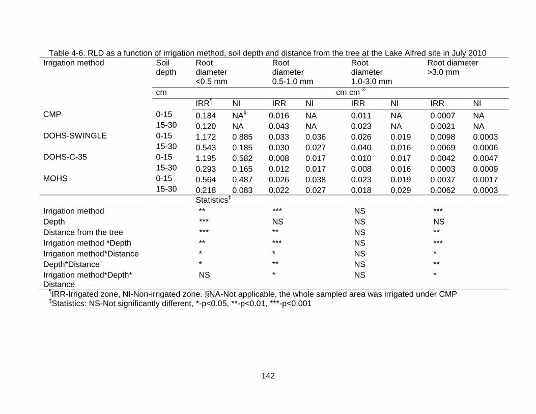
142
Table 4-6. RLD as a function of irrigation method, soil depth and distance from the tree at the Lake Alfred site in July 2010
Irrigation method Soil depth
Root diameter <0.5 mm
Root diameter 0.5-1.0 mm
Root diameter 1.0-3.0 mm
Root diameter >3.0 mm
cm cm cm-3
IRR¶ NI IRR NI IRR NI IRR NI
CMP 0-15 0.184 NA§ 0.016 NA 0.011 NA 0.0007 NA 15-30 0.120 NA 0.043 NA 0.023 NA 0.0021 NA DOHS-SWINGLE 0-15 1.172 0.885 0.033 0.036 0.026 0.019 0.0098 0.0003 15-30 0.543 0.185 0.030 0.027 0.040 0.016 0.0069 0.0006 DOHS-C-35 0-15 1.195 0.582 0.008 0.017 0.010 0.017 0.0042 0.0047 15-30 0.293 0.165 0.012 0.017 0.008 0.016 0.0003 0.0009 MOHS 0-15 0.564 0.487 0.026 0.038 0.023 0.019 0.0037 0.0017 15-30 0.218 0.083 0.022 0.027 0.018 0.029 0.0062 0.0003
Statistics‡
Irrigation method ** *** NS ***
Depth *** NS NS NS
Distance from the tree *** ** NS **
Irrigation method *Depth ** *** NS ***
Irrigation method*Distance * * NS *
Depth*Distance * ** NS **
Irrigation method*Depth* Distance
NS * NS *
¶IRR-Irrigated zone, NI-Non-irrigated zone. §NA-Not applicable, the whole sampled area was irrigated under CMP ‡Statistics: NS-Not significantly different, *-p<0.05, **-p<0.01, ***-p<0.001

143
Date
11/1/09 1/1/10 3/1/10 5/1/10 7/1/10
Canopy v
olu
me (
m3)
0.0
0.5
1.0
1.5
2.0
2.5
DOHS-Swingle
CMP
MOHS
DOHS-C35
Figure 4-1. Canopy volume as a function of fertilization practice at the Lake Alfred site. Error bars denote one standard deviation of 4 replications

144
August 2009 July 2010 August 2011
Cro
ss-s
ectio
nal a
rea
(cm
2 )
0
10
20
30
40
50
CMP
DOHS
MOHS
August 2009 CMP vs. DOHS NS
CMP vs. MOHS * DOHS vs. MOHS * N 12
July 2010 CMP vs. DOHS NS CMP vs. MOHS * DOHS vs. MOHS * N 60
August 2011 CMP vs. DOHS NS CMP vs. MOHS NS DOHS vs. MOHS NS N 60
*-indicates significance at p<0.05; NS-indicates non-significant differences; CMP-Conventional microsprinkler practice, DOHS-Drip open hydroponics system, MOHS-Microsprinkler open hydroponics system
Figure 4-2. Trunk cross-sectional area as a function of fertigation practice at the
Immokalee site. Error bars denote one standard deviation

145
Year
July 2010 August 2011
Can
op
y v
olu
me
(m3)
0
2
4
6
8
10
12
CMP
DOHS
MOHS
July 2010, August 2011 CMP vs. DOHS NS CMP vs. MOHS NS DOHS vs. MOHS NS N 60
Mean±one standard deviation, NS-Not significant, *-p<0.05, **-p<0.01, CMP-Conventional microsprinkler practice, DOHS-Drip open hydroponics system, MOHS-Microsprinkler open hydroponics system
Figure 4-3. Canopy volume as a function of fertigation method at the Immokalee site

146
Table 4-7. Trunk cross-sectional area as function of fertigation method at the Lake Alfred site
Fertigation method TCA-December 2009 TCA-July 2010 TCA-March 2011
cm2
DOHS-Swingle‡ 4.34±0.73 8.99±0.66 14.44±0.94
CMP¶ 4.37±1.66 6.51±0.61 10.02±1.55
MOHS 4.23±0.57 8.55±0.81 12.84±2.04
DOHS-C-35 4.71±0.56 9.82±0.39 12.83±1.50
Significance§ NS ** ** ‡Mean±one standard deviation, ¶CMP-Conventional microsprinkler practice, DOHS-Swingle-Drip open hydroponic system with Hamlins on Swingle rootstock, DOHS-C-35- Drip open hydroponic system with Hamlins on C35 rootstock, MOHS-Microsprinkler open hydroponic system, §NS-Not significant, **-p<0.01, TCA-Trunk cross-sectional area

147
CHAPTER 5 EFFECTS OF IRRIGATION METHOD AND FREQUENCY ON CITRUS WATER
UPTAKE AND SOIL MOISTURE DISTRIBUTION
Accurate estimation of plant water use could improve irrigation management
(Gutierrez et al., 1994; Morgan et al., 2006b) leading to a better understanding of plant-
water-interactions (Ham et al., 1990; Gutierrez et al., 1994). Plant water use typically
called crop evapotranspiration (ETc) can be determined with the stem heat balance
(SHB) method. The SHB technique has been found to be reasonably accurate and
dependable in estimating plant water use in pecan (Steinberg et al., 1990a, b), citrus
(Steppe et al., 2006), Anacardium excelsum (Meinzer et al., 1993), cotton (Ham et al.
1990), coffee and koa (Gutiérrez and Meinzer, 1994; Gutiérrez et al., 1994) and
grapevines (Lascano et al., 1992; Heilman et al., 1994). The SHB approach provides a
reliable method for measuring sap flow in the stems of herbaceous plants that is
sufficiently accurate for application in many agronomic and biological applications
(Baker and van Bavel, 1987; Baker and Nieber, 1989). Using the SHB method, sap
flow rates in trees have been found to be within 4 to 10% of transpiration loss (Baker
and Nieber, 1989; Steinberg et al., 1989; Lascano et al., 1992; Devitt et al., 1993).
Dugas et al. (1994) also showed that cumulative sap flow for 14-day periods was similar
to cumulative evapotranspiration or transpiration calculated from a water balance in
cotton. SHB technique has several advantages over other methods for measuring
water use such as lysimetry and water balance. The technique is non-intrusive, does
not require calibration, responds quickly to plant water flow, can be used over long
periods of time without damage to the plant (Baker and van Bavel, 1987; Steinberg et
al., 1989; Gutierrez et al., 1994) and is simple to use with an appropriate digital
datalogger (Baker and van Bavel, 1987).

148
Using reference evapotranspiration (ETo), ETc can be accurately determined once
a crop coefficient (Kc) and soil moisture depletion coefficient (Ks) are known (Allen et al.,
1998). Ks can be determined through periodic soil moisture measurement at selected
depths of the plant root zone (Morgan et al., 2006b; Fares et al., 2008). Kc is defined as
the ratio of crop evapotranspiration (ETc) to potential evapotranspiration (ETo) when soil
water availability is non-limiting and is a function of crop type, climate, soil evaporation
and crop growth stage (Allen et al., 1998; Morgan et al., 2006; Fares et al., 2008).
Several studies using water balance and drainage lysimeter methods estimated that Kc
values of citrus trees range from 0.6 in the fall and winter to 1.2 in the summer (Rogers
et al., 1983; Boman, 1994; Martin et al., 1997, Fares and Alva, 1999, Morgan et al.,
2006b). Jia et al. (2007) found that Kc values may vary from location to location. For
example, they found that annual average Kc values were higher for the citrus grown in
the Ridge regions (Kc =0.88) than for the Flatwoods (Kc = 0.72) in Florida, with monthly
recommended values ranging from 0.70 to 1.05 for the ridge and from 0.65 to 0.85 for
the Flatwoods citrus, respectively. They attributed the differences due to water logging
in the root zone of the Flatwoods citrus owing to water table due to the presence of the
spodic and/or argillic horizon. In studies on citrus Kc from other regions, different values
have been reported depending on climate and method used. Values ranging from 0.80
to 0.90 have been reported using the water balance technique (Allen et al., 1998). For
navel-orange tree groves in California, Consoli et al. (2006) found that Kc values ranged
from 0.45 to 0.93 using an energy balance method. Rana et al. (2005), using the eddy
correlation method, found that Kc values ranged from 0.8 to 1.2, corresponding to citrus

149
phenological growth stage and the effects of high wind speed and high vapor pressure
deficit.
Many studies in Florida on citrus tree water use have used other methods such as
lysimetry, water balance and the Florida Automated Weather Network (FAWN) to
estimate tree water use in citrus trees in the field without partitioning evaporation and
transpiration from the ET component (Rogers et al., 1983; Boman, 1994; Obreza and
Pitts, 2002; Jia et al., 2007; Morgan et al., 2006b; Fares et al., 2008). We attempted to
estimate tree water use using the SHB technique to calculate Kc values basing on plant
transpiration and Leaf Area Index (LAI) and correlate the two with root length density
(RLD) and canopy volume. Water use through hourly and daily sap flow measurements
would help in accurately predicting transpiration and devising ways of minimizing
evaporation and percolation losses by synchronizing irrigation applications with peak
tree water use. According to Morgan et al. (2006b), estimation of soil water uptake and
resulting soil water depletion would allow for a more accurate assessment of soil water
depletion, crop water uptake and soil moisture storage capacity.
The hypotheses postulated were:
1) citrus water use increases with canopy volume and root length density in-situ irrespective of the irrigation frequency and fertigation method and, that,
2) soil water content will be greater using the drip and microsprinkler OHS than grower practice.
The objectives of the study were to:
1) determine ETc and Kc using SHB method on 1.5- and 4-year old citrus using three different irrigation methods and fertigation frequencies on Florida Spodosol and Entisol;
2) determine soil water distribution in the citrus irrigated root zone.

150
Materials and Methods
Experimental design and irrigation methods
A randomized complete block design consisting of three treatments at Immokalee
site and two to four treatments at the Lake Alfred site was used, with three to four trees
serving as replications. The irrigation treatments were applied to the replicate trees
independently within a row. The irrigation treatments were as follows: (1) Conventional
practice (CMP) irrigated weekly, with the microsprinkler placed at about 10-15 cm
perpendicular to the tree; (2) Drip OHS (DOHS) – irrigated daily in small pulses, with
two drip lines spaced at 30 cm from the tree, each delivering four emitters on each side
of the tree; (3) Microsprinkler OHS (MOHS) – irrigated daily, with the microsprinkler
placed at about 15 cm perpendicular to the tree. All the treatments were replicated four
times. The treatments imposed at Lake Alfred were similar to the set-up at Immokalee
site except for the modification to DOHS that had one drip line placed within the tree
row, with one dripper placed at 15 cm on each side of the tree. The DOHS was imposed
on both Swingle and C35 rootstocks. Drip irrigation was provided with integral Uniram
(Netafim) pressure-compensating drip emitters (Netafim, Fresno, CA) (2.00 L h-1). At
both sites, microsprinkler irrigation was provided with either a single 40 L h-1 Max-14
(Maxijet, Dundee, FL) fill-in blue emitter for CMP or a 29 L h-1 Max-14 fill-in orange
emitter for MOHS at each tree (Schumann et al., 2009; 2010).
Estimation of Soil Moisture
Soil water sensors on Candler sand (VG400, Vegetronix, Sandy, UT) and
Immokalee sand (RS-485, Portland, OR), using the capacitance method (Katul et al.,
1997; Morgan et al.; 1999; 2002) of estimating volumetric water content were used to
measure moisture to determine treatment effects on soil water status. Soil moisture was

151
measured every 30 minutes at 10 cm and 45 cm depths on Candler sand and 10-, 20-,
30-, 40- and 50-cm depths on Immokalee sand using capacitance probes and an
automated logging system. Volumetric water content was measured (%) (Hillel, 1998).
Rainfall data and other climatic variables were collected from FAWN stations at
Southwest Florida Research and Education Center (SWFREC) and Citrus Research
and Education Center (CREC) (http://fawn.ifas.ufl.edu/) (Apprendix E).
Estimation of Crop Water Uptake and Kc
Actual transpiration was measured on tree trunks or branches with a heat-balance
method using Dynagage Flow32-1K Sap Flow System to evaluate tree water use. The
direct transpiration readings were taken from July 2010, March 2011 and August to
September 2011 at the Lake Alfred site and February, March and June 2011 at
SWFREC. Kc was estimated for each site using the measured citrus transpiration and
calculated reference ETo from FAWN data. Water uptake was measured using sap flow
sensors (Dynamax Inc., Houston, TX) on branches of four random trees per treatment
(each tree serving as a replicate) at SWFREC. At SWFREC, four healthy trees per
treatment were randomly selected to serve as replicates in the measurements.
At Lake Alfred, due to limitation in the size of sensors, sap flow measurements on
trunks of six trees were taken on Drip OHS (DOHS-Swingle) and Conventional
microsprinkler practice (CMP). Prior to installation of the sensors, measurements were
taken of branch and trunk diameter. Also, critical measurements of variables that
characterize water use in citrus such as Leaf Area Index (LAI) and canopy volume were
determined using a Leaf Area Meter and measuring tape. In the study, we used the
Dynamax Flow32-1K sap flow system (Dynamax Inc., Houston, TX) with CR1000 data
logger, including PC400 data logger support software (Campbell Scientific Inc., Logan,

152
UT). Trees at Lake Alfred had trunk diameters ranging from 24.92 mm to 31.40 and leaf
area index (LAI) was about 1.77±0.71 in July 2010. We used the gauges of SGB25
model at the Lake Alfred site on trunks in July 2010 because the tree trunks were
greater than 24 mm in diameter. In the subsequent seasons, the following sizes of
sensors were used: SGA13-ws, SGB16-ws, SGB19-ws and SGB25-ws for respective
stem diameter ranges of 12-16, 15-19, 18-23 and 24-32 mm. The thermocouple gaps
specified were: 4.0 for SGA13, 5.0 for both SGB16 and SGB19, and 7.0 for SGB25.
Tree canopy volumes were estimated by measuring the average canopy diameter
using canopy width in the east-west and north-south directions and canopy height using
the formula for a sphere=
r3, where r is the canopy radius. Trunk diameter was
estimated from averaging the diameter in the east-west and north-south directions and
then calculating the area using the formula r2, where r is the trunk radius.
We adapted the approach for determining sap flow measurements from individual
plants recommended by Lascano et al. (1992). Water use for trees was determined
from measurement of sap flow in limbs by increasing measured sap flow by the
proportion of leaf area of the measured limb over the leaf area of the entire tree. The
mean transpiration, was estimated by normalizing the stem flow data on a population
per land area basis as:
(
) (5-1)
Where is Esap=daily value of sap flow per unit land area (mm d-1), M=sap flow per
plant (kg d-1), P=plant population m-2 and ρwater is water density, 1000 kg m-3.

153
The index sapflow crop coefficient, Kc, was estimated following the equation below:
(
) (5-2)
where ETc is daily crop evapotranspiration (mm d-1), ETo is reference
evapotranspiraton (mm d-1), Esap is the daily value of sap flow per unit land area (mm d-
1), Ks is soil water stress coefficient. Thus, assuming no water stress due to the
automated irrigation, Ks, becomes unity.
The variation in soil water storage (ΔS) between two depths at the Lake Alfred site
(z1=0 cm and z2=45 cm) and Immokalee site (z1=0 cm, z2=10 cm, z3=20 cm, z4=30 cm,
z5=40 cm, z6=50 cm) for a given period of time (Δt=t1-t2; i.e., 1 day was used) was
calculated based on measured water content readings by the capacitance probes using
the following equation already formulated by Fares and Alva (2000b):
∫ ( )
∫ ( )
(5-3)
Results and Discussion
Tree characteristics at Immokalee and Lake Alfred
To determine leaf area in spring 2011, we categorized leaves at each site by size
and measured the leaf area, length and width. Leaf areas for small, medium and large
leaves averaged 10.7±4.2, 28.7±8.4, 67.4±16.8 cm2 at Immokalee. Leaf areas for small,
medium and large leaves averaged 15.1±4.7, 36.2±8.0, 68.9±16.0 cm2 at Lake Alfred
(Table 5-1). Tree canopy volumes ranged from 4.40±0.98 to 7.04±0.80 m3 in February
154
2011 and from 6.67±1.30 to 9.32±1.10 in June 2011 at Immokalee (Table 5-2). At the
Lake Alfred site, tree canopy measurements showed that canopy volumes ranged from
0.90±0.20 to 1.42±0.32 m3 in July 2010, 2.81±0.73 to 4.89±0.58 in March 2011 and
4.45±0.45 to 6.53±0.88 in August 2011 (Table 5-2). Trunk cross-sectional areas varied
from 19.32±4.35 to 27.00±2.14 cm2 in February 2011 and 25.72±3.92 to 31.51±2.32
cm2 in June 2011 at Immokalee. Trunk cross-sectional areas varied from 5.59±1.17 to
7.06±0.26, 10.02±1.55 to 14.44±0.94 cm2 in March 2011 and 18.19±2.01 to 25.59±1.94
cm2 in August 2011 at Lake Alfred (Table 5-2). To estimate, leaf areas in later sap flow
studies, we developed calibration equations as shown in Figures 5-1 and 5-2.
Water Uptake at Immokalee and Lake Alfred
On average most days, we observed no sap flows in the two treatments at 0, 1, 6,
7, 8, 22 and 23 h as exemplified in Figure 5-3 in July 2010. Peak sap flow readings
were noted between 10 and 20 h, ranging from 134 to 220 g h-1 under DOHS-Swingle.
Sap flow readings under CMP peaked between 11 and 19 h, ranging from 110 to 133 g
h-1. In March 2011, average hourly sap flows peaked at around 1100 h and 1200 h. On
March 17, 2011, for example, peak sap flows recorded were 298, 329, 519 and 336 g h-
1 for DOHS-Swingle (at 1400 h), CMP and DOHS-C35 (at 1300 h), and MOHS (at 1200
h), respectively. On average hourly sap flow in March ranged from 194±35 to 385±152
g h-1, 117±36 to 297±33 g h-1, 176±32 to 276±46 g h-1 and from 154±26 to 248±46 g h-1
for DOHS-C35, MOHS, DOHS-Swingle and CMP (Figure 5-3). Similar to observations
in July 2010, we noted that sap flows in spring 2011 also showed consistently high
readings (>100 g h-1) between 1000 h and 1800 h, probably due to increased solar
radiation (averaging 239 and 254 W m-2 in July 2010 and March 2011) and temperature
(25-30 oC in July 2010 and 11-22 oC March 2011) compared with the rest of day.

155
Similar hourly sap flows among the treatments using Swingle rootstock (DOHS-Swingle,
MOHS, CMP) were noted regardless of the fertigation method and irrigation frequency
(Figure 5-3). However, DOHS on C35 rootstock, had peak hourly sap flows that were
58% to 61% higher than CMP.
Lowest daily sap flow was approximately 2.05 kg d-1 on July 12, 2010 while the
highest sap flow was about 4.74 kg d-1 on July 18, 2010 under DOHS-Swingle with
mean daily sap flow readings averaging 3.96±0.74 g d-1 (Figure 5-4). Using CMP, the
maximum and minimum values of the average daily sap flows were about 3.83 kg d-1
and 1.71 kg d-1 on July 10 and July 25, 2010, respectively, with a mean of 2.75±0.59 kg
d-1 (Figure 5-4). There was very high variability in the daily readings of grower practice
as shown in Figure 5-4 while consistently high readings with less variability were
observed using DOHS-Swingle. On average, the sap flow was 44% higher under
DOHS-Swingle than CMP. It appears the trees under grower practice also had some
reasonable variability in trunk cross-sectional area (Table 5-2). Lascano et al. (1992), in
their study on grapevines, explained that such variability among trees exists and can be
reduced by normalizing the total sap flow by leaf area. Furthermore, in March 2011, all
DOHS treatments on Swingle and C35 rootstocks showed sap flows greater than CMP
by 7 to 150%. Sap flow for MOHS was higher than CMP on all days except on Julian
days 77 and 78 when daily sap flow was 6% less than CMP suggesting that significant
gains in water uptake on the ridge soil lie with drip OHS (Figure 5-5). In March 2011,
daily transpiration readings were lowest using CMP on March 11, 2011 and peaked on
March 23, 2011 using DOHS-C35 ( Figure 5-5). Lowest average daily sap flows were
observed on 03/11/2011 at the beginning of the study. For example, sapflows for CMP,

156
DOHS-Swingle, DOHS-C35 and MOHS averaged 1.19±0.18, 2.77±1.42, 2.96±1.95 and
2.77±0.90 kg d-1, respectively. Average daily sap flows for the all the treatments but
CMP at Lake Alfred peaked on 03/23/2011. CMP showed a peak average sap flow of
4.84±0.94 kg d-1 on 03/18/2011. Peak sap flows recorded for DOHS-Swingle, DOHS-
C35 and MOHS were 5.73±1.42, 8.98±7.28 and 4.71±2.37 g d-1.
Average hourly and daily sap flows readings for studies conducted at SWFREC in
February and March 2011 are given in Figures 5-6 and 5-7. For MOHS and CMP, we
noted very low sap flow readings. The statuses of sensors reportedly ranged from 5-7
showing faulty readings that were identified late in the study. DOHS averaged hourly
sap flow peaked to 1,361 g h-1 at 1100 h on February 27, 2011. MOHS and CMP
peaked to about 210 g h-1 on February 27 at 1000 h. The data logger used for MOHS
and CMP showed no readings most of the time resulting in the extremely low readings.
We had to get this fixed at the end of the experiment. Thus, the readings for DOHS
might actually represent the SWFREC site. Daily sap flow peaked to 21.6 kg d-1 on
March 3, 2011 using DOHS. As indicated above, we also observed very low readings
for MOHS with maximum daily sap flow of 1.38 kg d-1 and for CMP where maximum
daily sap flow was 1.09 kg d-1. Minimum daily sap flow readings were 213 and 220 g d-1
for MOHS and CMP, respectively.
Average hourly sap flows (Figure 5-8) in June 2011 at SWFREC was high
between 1000h and 1600h in all the three fertigation methods peaking to respective
values of 3.55, 2.27 and 1.77 kg h-1, for DOHS, MOHS and CMP at 1600 h, 1400 h and
1300 h, respectively. Hourly sap flows peaked between 1000 h and 1900 h for DOHS
and CMP, and between 1000 h and 2000 h for MOHS.

157
The average hourly sap flows at the Lake Alfred site in August- September 2011
(Figure 5-9), peaked between 1000 h and 1700 h. Sap flows followed the pattern
DOHS- Swingle>MOHS> CMP>DOHS-C35. DOHS- Swingle, MOHS and CMP peaked
to 2.53 kg h-1, 1.62 kg h-1, and 1.19 kg h-1 at 1400 h and DOHS-C35 peaked to 0.85 kg
h-1 at 1300 h. The trees for the Swingle rootstock, including the grower practice (see
canopy volumes in Table 5-2), had grown so much in fall 2011 compared with March
2011 at the Lake Alfred site with trunk cross-sectional area increments of 66, 77 and
94% and canopy volume increments of 49, 34 and 90% for the MOHS, DOHS and
CMP, respectively. The grower practice, CMP, had the largest increase in canopy
volume and significant increase in leaf area, probably due to the use of controlled-
release fertilizer in summer 2010 and 2011. The tree size for C35 rootstock did
increase by only 16 and 42% in canopy volume and trunk cross-sectional area
suggesting a small increase in leaf area.
DOHS hourly sap flow was well above the other two fertigation methods in June
2011 at SWFREC. Daily sap flows (Figure 5-10) peaked in the following order: DOHS >
MOHS ≈ CMP with respective maxima and minima of 58.8±28.7 and 33.3±1.7 kg d-1,
33.8±16.6 and 23.5±10.6 kg d-1, and 26.6±14.2 kg d-1 and 14.5±11.4 kg d-1. All sap
flows for DOHS ranged from 87 to 160% while for MOHS daily sap flow were 10 to
103% greater than CMP.
In August-September 2011, daily sap flow averaged 35, 27, 14 and 13 kg d-1 for
DOHS-Swingle, MOHS, DOHS-C35, and CMP suggesting increments by 176%, 130%
and 16% over CMP at the Lake Alfred site. As explained above we expected much
higher sap flows for DOHS-C35 but a small increase in tree size and, probably leaf area

158
compared with the other irrigation methods resulted in lower sap flow values compared
with observations in March 2011 (Figure 5-11).
Daily sap flows per unit land area in July 2010 ranged from 0.11 to 0.25 mm d-1
using DOHS-Swingle and 0.09 to 0.21 mm d-1 using CMP with respective averages of
0.21 and 0.15 mm d-1 (Appendix A, Figure A36). Sap flows for the Swingles ranged from
0.20 to 0.31 mm d-1 and from 0.28 to 0.39 mm d-1 for DOHS-C35 in March 2011 at the
Lake Alfred site (Appendix A, Figure A37). The sap flow in February-March 2011at
Immokalee averaged 0.81 mm d-1 peaking to 1.06 mm d-1 on Julian day 61 (Appendix A,
Figure A38). In June 2011 at Immokalee daily sap flow averaged 2.3, 1.4 and 1.1 mm
d-1 for DOHS, MOHS and CMP (Appendix A, Figure A39). In August-September 2011
at the Lake Alfred site, daily sap flow ranged from 1.03±0.67 to 2.80±2.21 mm d-1,
0.23±0.08 to 1.11±0.42 mm d-1, 0.74±0.03 to 1.97±0.28 mm d-1, and 0.62±0.21 to
1.38±0.64 mm d-1 for DOHS-Swingle, CMP, MOHS and DOHS-C35 (Appendix A, Figure
A40). Large canopies, leaf areas and increased temperatures (averaging 26 oC at both
Immokalee and the Lake Alfred site) accounted for better uptake in the OHS fertigation
methods than grower practices at both sites.
Cumulative sap flows at the Lake Alfred site on the studies undertaken between
Julian days 190-209 in 2010, 70-82 and 236-251 in 2011 showed that DOHS-Swingle
had cumulative sap flow of 4.3 mm on day 209 while cumulative sap flow of CMP was
3.0 mm representing percent increase in sap flow in DOHS-Swingle of 20 to 56% over
CMP between Julian days 190 and 209 (Appendix A, Figure A41). Cumulative sap
flows were 43%, 35% and 80% higher than CMP for DOHS-Swngle, MOHS and DOHS-
C35 representing very high uptake using ACPS fertigation compared with conventional

159
irrigation practice between Julian days 70 and 82 (Appendix A, Figure A42). The
cumulative sap flows were 3.34, 2.58, 3.01 and 4.75 mm for DOHS-Swingle, CMP,
MOHS and DOHS-C35 between Days 70 and 82. In August-September 2011, the trees
had increased in trunk cross-sectional area, canopy volume and leaf area resulting in
cumulative sap flows that were 166%, 141% and 65% higher than CMP using DOHS-
Swingle, MOHS and DOHS-C35, respectively. The cumulative sap flows on Julian Day
251 peaked to 30, 11, 23 and 17 mm using DOHS-Swingle, CMP, MOHS and DOHS-
C35 (Appendix A, Figure A43).
In March 2011 at Immokalee, DOHS-Swingle peaked from 0.77 mm on Julian
Day 48 to 11.31 mm on day 61 (Appendix A, Figure A44). The cumulative sap flows of
44 mm and 27 mm using DOHS and MOHS in June 2011 representing, on average,
115% and 37% higher sap flows than CMP, underlining the importance of frequent
fertigation as also shown on the ridge site (Appendix A, Figure A45).
Index sap flow Kc averaged 0.029±0.014 and 0.042±0.003 using CMP and DOHS-
Swingle, respectively at the Lake Alfred site in July 2010 (Appendix A, Figure A46),
increasing to 0.06±0.01 and 0.08±0.02 in March 2011 (Appendix A, Figure A47). In
March 2011, Kc values for MOHS and DOHS-C35 were 0.07±0.04 and 0.11±0.09
(Appendix A, Figure A47). The average Kc peaked in August-September ranging from
0.21±0.06 to 0.57±0.43, with high Kc observed in the OHS irrigation methods compared
with grower practice probably because of frequent irrigation, vigorous tree growth and
large canopies (Appendix A, Figure A48). At SWFREC, sap flow Kc ranged from
0.25±0.10 to 0.34±0.15 in February-March 2011 (Appendix A, Figure A49). The Kc in
June 2011, ranged from 0.30±0.11 to 0.54±0.26, 0.21±0.09 to 0.34±0.14 and 0.13±0.10

160
to 0.25±0.15 using DOHS, MOHS, and CMP, respectively, suggesting that water uptake
followed the order DOHS>MOHS>CMP (Figure A50). The sap flow Kc for the <2.5 yr-old
trees at the Lake Alfred site suggests that transpiration accounted for about 3 to 10% of
the actual evapotranspiration because the trees were young with small canopy volumes
(ranging from 0.71 to 1.72 m3) and leaf area (LAI ranged from 1.23±0.42 to 2.30±0.49)
and thus had little ground cover. Soil evaporation tends to account for the greatest part
of actual transpiration for a uniformly wetted surface not covered by the canopy (Testi et
al., 2004). With trees getting older ~3 years or older, the transpiration component, as
expected, increased and accounted for about 25 to 70% of the actual
evapotranspiration. This is because citrus Kc for Florida conditions ranges from 0.6 in
the fall and winter to 1.2 in the summer (Rogers et al., 1983; Boman, 1994; Fares and
Alva, 1999; Morgan et al., 2006b; Jia et al., 2007) and water use tends to increase with
age and increase in canopy volume (Morgan et al., 2006b). It is important to assess
actual tree water use for proper irrigation scheduling and planning because, depending
on tree age, water may need to be applied in the actual root zone for tree uptake as was
the case with the OHS treatments. The sap flow Kc values in June/July and
August/September (for trees>3 yr-old) are close to or slightly lower than many crop
coefficients from other regions that included the evaporation component (Hoffman et al.,
1982; Castel et al., 1987; Sepaskhah and Kashefipour, 1995; Martin et al., 1997;
Consoli et al., 2006; Petillo and Castel, 2007; Snyder and O’Connell, 2007) or split the
evaporation and transpiration components (Villalobos et al., 2009). Our study focused
on trees <5 yr-old young trees while the studies from the other regions above focused
on trees >7-yr-old mature trees. Rogers et al. (1983) explained that frequent rains in

161
Florida produce wet soil and leaf conditions that result in the actual ET being a great
percentage of the potential ET than is true for semi-arid or arid conditions of California,
USA (Consoli et al., 2006; Snyder and O’Connell, 2007), Texas, USA (Hoffman et al.,
1982), Arizona, USA (Martin et al., 1997), Iran (Sepaskhah and Kashefipour, 1995),
Japan (Yang et al., 2003; 2010) and Spain (Castel et al., 1987; Testi et al., 2004;
Villalobos et al., 2009). This suggests that, ceteris paribus, Florida does have high water
evaporative demand due to the hot humid climate and the deep drainage ascribed to
the sandy soil characteristic.
Soil moisture distribution at Lake Alfred and Immokalee
The soil moisture distribution pattern showed that there was ample soil moisture in
the root zone in all the treatments in July 2010 at the Lake Alfred site. For example,
average soil moisture measurements as shown by time of day using grower practice
(CMP) show that maximum soil moisture content was 8.42% (at 17.0 h) and minimum of
6.31% (at 15.8 h) at 10 cm soil depth layer and a maximum of 9.02% (at 18.0 h) and a
minimum of 6.88% (at 15.8 h) at the 45 cm soil depth layer. MOHS yielded maximum
soil moisture of 13.65% (at 9.8 h) and a minimum of 8.98% (at 8.0 h) at10 cm soil depth
and 12.02% (at 17.5 h) and 11.26% (at 9.3 h) at 45 cm soil layer. The maxima and
minima soil moisture using DOHS-C35 were 19.50% (at 8.5 h) and 9.99% (at 13.0 h) at
10 cm soil depth and 12.43% (at 17.5 h) and 11.65% (around 8.3-8.8 h) at 45 cm soil
depth (Figure 5-12). Daily soil moisture at 10 and 45 cm soil depths averaged 7.6±1.6
and 8.2±0.9%, 10.2±3.2 and 11.5±0.8%, and 11.8±4.5 and 12.0±0.4% (Figures 5-13
and 5-14) using CMP, MOHS and DOHS-C35. Lower average soil moisture content at
10 cm than 45 cm suggests water removals either through tree uptake, soil evaporation
or downward drainage.

162
In March 2011 at the Lake Alfred site, the soil moisture peaked to around 8.22,
12.08 and 14.79% between 7.30am and 8.30am at 10 cm depth, decreased to 6.44,
10.86 and 7.18% in the afternoon and at night in the respective treatments CMP,
MOHS, DOHS-C35 (Figure 5-15). At 45 cm soil depth, soil moisture was higher than
the upper top 10 cm soil layer (Figure 5-15) probably due to downward drainage. Daily
soil moisture averaged 7.3, 11.3 and 10.5% at 10 cm depth (Figure 5-16) and 10.5, 12.3
and 7.6% at 45 cm depth (Figure 5-17) using CMP, MOHS and DOHS-C35 irrigation
treatments in March 2011. Our own results in Chapter 4 and those of Zhang et al.
(1996) confirm that tree uptake should be greater in the 0-15 cm soil layer than lower
horizons owing to high root density in the range of 55-67% on length basis (this study)
and 70-75% on weight basis (Zhang et al., 1996) in the top 15 cm. Our observations
are also supported by earlier studies (Goldberg et al., 1971; Alva and Syvertsen, 1991;
Khan et al. 1996; Alva et al., 1999; Fares and Alva, 2000a, b; Badr, 2007; Davenport et
al., 2008; Badr and Abuarab, 2011). Khan et al. (1996) showed that soil water content
increased up to 25 cm depth and 30 cm radial distance at application rates ranging from
1.5-2.5 L h-1 and input concentration falling between 100 and 500 mg L-1 on coarse
loamy soil. They also showed that solute concentration increased with high input
concentration, applied volume and application rate up to about the same depth (~25 cm)
and radial distance (~30 cm) as for soil water content. Davenport et al. (2008) further
observed that soil moisture distribution for drip-irrigated vineyards was adequate in the
0-45 cm depth and within 20-40 cm radius, either diagonal or perpendicular to the drip
line. Our observations are also supported by Goldberg et al. (1971) who concluded in
their study that soil moisture resulting from drip irrigation was two dimensional, with

163
moisture contents high along and beneath the row and decreasing laterally. Thus,
according to Goldberg et al. (1971) the effect of shorter irrigation intervals, as was the
case with drip and microsprinkler ACPS/OHS, with proportionally smaller amounts of
water applied in a single irrigation, is to decrease the variations in moisture content in
the root zone and establish a continuously higher moisture regime. Eventually, drip that
was developed to conserve water in arid environments (Goldberg and Shmueli, 1970)
has been adapted to semi-arid and humid regions to manage water in sandy soils with
high conductivity and supplement water where rainfall is inadequate or is not uniformly
distributed throughout the year.
In August and September 2011, a contrary soil moisture distribution trend was
noted. The moisture content averaged 12.63 and 10.94% (CMP), 10.88 and 8.06%
(MOHS) and 11.55 and 9.32% (DOHS-C35) at 10 cm and 45 cm depth layers,
respectively, suggesting that soil moisture decreased with depth probably because of
the frequent rainfall that kept the top 10 cm layer wet throughout the study period
(Figures 5-18, 5-19 and 5-20).
On Immokalee sand, the DOHS soil moisture varied between 7.5 and 10.0% in the
top 10-30 cm and remained between 5 and 6.5% at 40- and 50 cm depths in February
and March 2011 (Figure 5-21). In June 2011, the moisture contents ranged from 7.5 to
12.0% in the top 30% and between 6.5 and 7.7 at 40- and 50-cm soil depths (Figure 5-
22). The soil water at Immokalee using MOHS ranged from 8.5 to 14% and around 6 to
8% in the 40 to 50 cm soil depths in February-March 2011 (Figure 5-23) and June 2011
(Figure 5-24). The grower practice had soil moisture contents varying between 8 and
13% in the top 20 cm, and between 6 and 7% in the 30-50 cm soil depth layers in

164
February-March 2011 (Figure 5-25). In June 2011, the soil moisture varied from 10-20%
in the top 20 cm and ranged from 6 to 13% in the lower 30-50 cm soil depth (Figure 5-
26). The lower soil moisture contents in the lower 30-50 cm depth suggests that
probably root water extraction in the top 30 cm resulted in less water percolating to
lower soil depth layers. This might hold because the Immokalee sand has a shallow
water table (Obreza and Pitts, 2002) that limits root development in the top 30 cm
(Bauer et al., 2004).
Factors affecting water uptake on the two soils
Linear and nonlinear analysis revealed the major factors controlling cumulative
water uptake for young citrus trees at Lake Alfred and Immokalee sites. In July 2010,
when the trees at the Lake Alfred site were fairly small (<2 yr-old) with small canopies
(<1.74 m3), cumulative water uptake was largely a function of trunk cross-sectional area
(R2=0.98, p<0.001) and canopy volume (R2=0.67, p=0.046) and less influence from soil
water, leaf area and root length density (R2<0.56, p>0.05) (Table 5-3). At about 2.5
years, the trees at Lake Alfred showed that soil water at Lake Alfred (p<0.001)
influenced water uptake to a larger extent while canopy volume, soil water at 45 cm,
trunk cross-sectional area and leaf area were less influential (p>0.05) (Table 5-4). This
observation was also supported by results for 6 yr-old trees at Immokalee in June 2011
and 3 yr-old trees at Lake Alfred later in September 2011. For example, cumulative
water uptake at Immokalee was largely influenced by soil water at 10, 20, 30, 40 and 50
cm soil depth (p<0.001) and not necessarily canopy volume (p=0.400), leaf area
(p=0.96) and trunk cross-sectional area (p=0.576). Also, the soil water at 10 cm
(p=0.001) and 45 cm (p=0.002) depths at Lake Alfred in September 2011 exerted
significant influence on water uptake compared with canopy volume (p=0.826), trunk

165
cross-sectional area (p=0.053) and leaf area (R2=0.27) (Tables 5-3 and 5-4). However,
longterm analysis of water uptake versus tree characteristics suggests that canopy
volume (Figure 5-27) will be the major determinant of overall tree water uses matched
with good irrigation practice. An exponential model adequately described the
relationship between cumulative water uptake and canopy volume. Thus, it appears for
young trees (<6 yr-old) irrigation scheduling is a critical management practice especially
for the sandy soil as shown by the good correlation with water uptake. Despite weak
correlation with root length density, the results on root density showed increased root
intensity in the top 0-30 cm soil depth layer indicating that water extraction would be
enhanced with an increase in available water.
Summary
The chapter described the citrus water uptake and soil moisture distribution
patterns in the irrigated zone on the citrus producing regions of central and southwest
Florida. The results showed that hourly, daily and cumulative sap flow were higher
using the ACPS/OHS irrigation methods compared with the conventional grower
practices (fertigated or receiving granular fertilization), albeit, not significantly different.
The citrus water use, in agreement with the postulated hypothesis, did increase with
canopy volume and root length density in-situ irrespective of the irrigation frequency and
fertigation method and correlated strongly with soil moisture content, trunk crossectional
area and canopy volume. The high uptake in the ACPS/OHS irrigation methods is
ascribed to the frequent irrigation and vigorous growth resulting in trees with large
canopy volumes, leaf areas and trunk cross-sectional areas compared with weekly
irrigation associated with the grower practice. The results support the thinking behind
the novel ACPS/OHS practices that nutrient leaching would be minimized while

166
accelerating tree growth as a result of enhanced water and corresponding nutrient
uptake. Thus, the irrigated root zones of DOHS or MOHS which have about 4% and
20% of the area irrigated by CMP, respectively, showed that the trees would not be
stressed by the ACPS practices.
The Kc followed a similar pattern to that of sap flow and was generally higher using
drip OHS compared with microsprinkler irrigation. For young trees 1.5 to 2.3 yr-old at
the Lake Alfred site, index sap flow Kc averaged 0.029±0.014 and 0.042±0.003 using
CMP and DOHS-Swingle, respectively at the Lake Alfred site in July 2010, increasing to
0.06±0.01 and 0.08±0.02 in March 2011. For older trees greater than 3 yr-old, Kc varied
from 0.25±0.10 in March, to 0.54±0.26 in June and 0.57±0.43 in September. Thus,
these studies revealed that tree water uptake accounted for about 3 to 10% of the
actual ET when the trees are small and over 60% of the ET after three years when the
trees increased in size with regard to leaf area and canopy volume.
The soil moisture distribution patterns in all the irrigation methods were similar and
maintained soil moisture close to or slightly above field capacity largely in the range of 7
and 15% suggesting that soil moisture was non-limiting at both sites. Thus, the
hypothesis that ‘drip and microsprinkler OHS would result in greater soil water content
in the irrigated zone than grower practices’ was not true. The increased availability of
water in the top 30 cm suggests that the leaching threat is minimal under such frequent
irrigation practices due to increased root water and probably nutrient extraction from this
layer. These results support intensive irrigation management practices in young trees to
insure ample water is available in the root zone.

167
Table 5-1. Average leaf area
Site Small Medium Large
cm2
Immokalee §10.71±4.19 28.68±8.39 67.27±16.77 Lake Alfred 15.13±4.70 36.22±8.04 68.93±16.01 §All values are mean areas of 20 leaves ± one standard deviation
Table 5-2. Tree canopy volume (CV), stem cross-sectional area (SCA), and trunk cross-sectional area (TCA)
Immokalee site
Irrigation method February 2011 June 2011
CV (m3) SCA (cm2) TCA (cm2) CV (m3) SCA (cm2) TCA (cm2)
DOHS ‡7.04±0.80 2.48±0.96 27.00±2.14 9.32±1.10 3.30±1.24 31.51±2.32 MOHS 4.40±0.98 2.34±0.80 19.32±4.35 6.67±1.30 3.47±1.43 26.19±4.44 CMP 6.47±1.20 2.05±0.81 20.21±2.60 7.61±1.26 3.09±1.23 25.72±3.92
Lake Alfred site
Irrigation method July 2010 March 2011 August 2011
CV (m3) TCA (cm2) CV (m3) TCA (cm2) CV (m3) TCA (cm2) ¶DOHS-Swingle 1.42±0.32 7.06±0.26 4.89±0.58 14.44±0.94 6.53±0.88 25.59±1.94 CMP 0.90±0.20 5.59±1.17 2.81±0.73 10.02±1.55 5.33±0.48 19.46±1.60 MOHS NA NA 3.91±0.67 12.84±2.04 5.84±0.85 21.33±3.41 DOHS-C-35 NA NA 3.83±0.79 12.83±1.50 4.45±0.45 18.19±2.01 ‡Mean±one standard deviation, n=3 per treatment for trees sampled in July 2010, n=4 for trees sampled in February, March and August 2011, mean ± 1 standard deviation, ¶CMP-Conventional microsprinkler practice, DOHS-Swingle-Drip open hydroponic system with Hamlins on Swingle rootstock, DOHS-C-35- Drip open hydroponic system with Hamlins on C-35 rootstock, MOHS-Microsprinkler open hydroponic system

168
Total leaf area (m2)
0 2 4 6 8 10 12
Leaf
are
a in
dex
0
1
2
3
4
LAI vs Total leaf area
Plot 1 Regr
Cano
py v
olum
e (m
3 )
0
1
2
3
4
5
6
Canopy volume vs Total leaf area
Plot 1 Regr
Y=0.26X+0.46, R2=0.59
Y=0.21X+2.30, R2=0.25
Figure 5-1. Linear correlations of leaf area index and canopy volume as a function of leaf area in March 2011 at the Lake Alfred site

169
Total leaf area (m2)
0 2 4 6 8 10 12 14 16 18 20
Lea
f ar
ea i
nd
ex
0
1
2
3
4
LAI vs Total leaf area
Plot 1 Regr
Can
opy
vol
um
e (m
3 )
0
2
4
6
8
10
Canopy volume vs Total leaf area
Plot 1 Regr
Y=0.16X+4.76, R2=0.16
Y=0.18X+0.59, R2=0.80
Figure 5-2. Correlations of leaf area index (LAI) and canopy volume as a function of
total leaf area at Immokalee site in March 2011

170
Ave
rag
e h
ou
rly
sap
flo
w (
g h
-1)
0
50
100
150
200
250
DOHS
CMP
Time (h)
0 5 10 15 20 25
0
100
200
300
400
500
600 DOHS-Swingle
CMP
DOHS-C35
MOHS
Figure 5-3. Average hourly sap flow in July, 2010 (top) and March, 2011 (bottom) at Lake Alfred site

171
Julian Day
190 195 200 205 210
Dai
ly s
apfl
ow
(g
d-1
)
0
2000
4000
6000
8000
DOHS-Swingle
CMP
Figure 5-4. Average daily sap flow in July, 2010 at the Lake Alfred site. Error bars represent one standard deviation
Julian Day
70 72 74 76 78 80 82
Ave
rage
dai
lysa
p flo
w (k
g d-1
)
0
2
4
6
8
10
12
14
16
18
DOHS-Swingle
CMP
DOHS-C35
MOHS
Figure 5-5. Average daily sap flow in March, 2011 at the Lake Alfred site. Error bars represent one standard deviation

172
Figure 5-6. Average hourly sap flow in February-March 2011 at SWFREC. Data logger used for CMP and MOHS had a fault and showed very low sap flow readings
Time (h)
0 5 10 15 20 25
0
200
400
600
800
1000
1200DOHS
Avera
ge h
ou
rly s
ap
flo
w (
g h
-1)
0
20
40
60
80
100
120
140
160
180
200
MOHS
CMP

173
0
1000
2000
3000MOHS
CMP
Julian Day
48 50 52 54 56 58 60 62
Average d
ail
y s
ap
flow
(g
d-1
)
0
10000
20000
30000
Daily sapflow-DOHS
Figure 5-7. Average daily sap flow in February-March 2011 at SWFREC. Error bars
represent one standard deviation. Data logger used for CMP and MOHS had a fault and showed very low sap flow readings

174
Time (h)0 5 10 15 20
0
1000
2000
3000
4000
5000
DOHS
MOHS
CMP
Ave
rage
hou
rly s
apflo
w (g
h-1
)
Figure 5-8. Average hourly flow in June 2011 at the Immokalee site

175
Time (h)
0 5 10 15 20
Avera
ge h
ourly s
ap f
low
(g h
-1)
0
1000
2000
3000
4000
DOHS-Swingle
CMP
MOHS
DOHS-C35
Figure 5-9. Average hourly sap flow in August-September, 2011 at the Lake Alfred site

176
Julian day
154 156 158 160 162 164 166 168 170 172
Da
ily s
ap
flo
w (
kg
d-1
)
0
20
40
60
80
100
DOHS
MOHS
CMP
Figure 5-10. Average daily sap flow in June 2011 at the Immokalee site. Error bars represent one standard deviation

177
Julian day
236 238 240 242 244 246 248 250 252
Daily
sapflow
(kg d
-1)
0
20
40
60
80
100
120
DOHS-Swingle
CMP
MOHS
DOHS-C-35
Figure 5-11. Average daily sap flow in August-September, 2011 at the Lake Alfred site.
Error bars represent one standard deviation

178
6
8
10
12
14
16
18
20
22
CMP-10 cm
MOHS-10 cm
DOHS-C35-10 cm
So
il m
ois
ture
(%
)
Time (h)
0 5 10 15 20
6
8
10
12
14
16
18CMP- 45 cm
MOHS-45 cm
DOHS-C35-45 cm
Figure 5-12. Average hourly soil moisture distribution in July 2010 at the Lake Alfred site
measured at 10- and 45 cm soil depth layers

179
Julian day
188 190 192 194 196 198 200 202 204 206
Volu
metr
ic s
oil
mois
ture
(%
)
0
5
10
15
20
25
CMP at 10cm
MOHS at 10cm
DOHS-C35 at 10cm
Figure 5-13. Average daily soil moisture distribution in July 2010 at the Lake Alfred site
measured at 10 cm soil depth layer. Error bars denote one standard deviation
Julian day
188 190 192 194 196 198 200 202 204 206
Volu
metr
ic s
oil
mois
ture
(%
)
6
8
10
12
14
16
CMP at 45cm
MOHS at 45cm
DOHS-C35 at 45cm
Figure 5-14. Soil moisture distribution in July 2010 at the Lake Alfred site measured at
45 cm soil depth layer. Error bars denote one standard deviation

180
Volu
metr
ic w
ate
r conte
nt
(%)
6
8
10
12
14
16
CMP-10cm
MOHS-10cm
DOHS-C35-10cm
Time (h)
0 5 10 15 20
Volu
metr
ic w
ate
r conte
nt
(%)
4
6
8
10
12
Figure 5-15. Average hourly soil moisture distribution at the Lake Alfred site measured
at 10 cm (top) and 45 cm (bottom) soil depth layers in March 2011.

181
Julian day
68 70 72 74 76 78 80 82 84
Volu
metr
ic w
ate
r conte
nt
(%)
0
5
10
15
20
25
CMP
MOHS
DOHS-C35
Figure 5-16. Daily soil moisture distribution at the Lake Alfred site measured at 10 cm soil depth layer in March 2011. Error bars denote one standard deviation
Julian day
68 70 72 74 76 78 80 82 84
Volu
metr
ic w
ate
r conte
nt
(%)
0
5
10
15
20
CMP
MOHS
DOHS-C35
Figure 5-17. Daily soil moisture distribution at the Lake Alfred site measured at 45 cm soil depth layer in March 2011. Error bars denote one standard deviation

182
Volu
metr
ic w
ate
r conte
nt
(%)
4
6
8
10
12
14
16
18
CMP-10 cm
MOHS-10 cm
DOHS-C35-10 cm
Time (h)
0 5 10 15 20
Volu
metr
ic w
ate
r conte
nt
(%)
4
6
8
10
12
14 CMP-45 cm
MOHS-45 cm
DOHS-C35-45 cm
Figure 5-18. Average hourly soil moisture distribution at the Lake Alfred site measured at 10- and 45 cm soil depth layers in August-September 2011

183
Julian day
234 236 238 240 242 244 246 248
Volu
metr
ic w
ate
r co
nte
nt
(%)
0
5
10
15
20
25
CMP
MOHS
DOHS-C35
Figure 5-19. Average daily soil moisture distribution at the Lake Alfred site measured at 10 cm soil depth layer in August-September 2011. Error bars denote one standard deviation

184
Julian day
234 236 238 240 242 244 246 248
Volu
metr
ic w
ate
r conte
nt
(%)
0
2
4
6
8
10
12
14
16
18
20
22
CMP
MOHS
DOHS-C35
Figure 5-20. Average daily soil moisture distribution at the Lake Alfred site measured at 45 cm soil depth layer in August-September 2011. Error bars denote one standard deviation

185
Julian day
44 46 48 50 52 54 56 58 60 62 64
Vol
umet
ric s
oil m
oist
ure
(%)
5
6
7
8
9
10
11
12
10 cm
20 cm
30 cm
40 cm
50 cm
Figure 5-21. Soil moisture distribution for DOHS in February-March 2011 at Immokalee
site measured at 10-, 20-, 30-, 40- and 50 cm soil depth layers. Error bars denote one standard deviation

186
Julian day
155 160 165 170
Volu
metr
ic m
ois
ture
conte
nt
(%)
6
8
10
12
14
10 cm
20 cm
30 cm
40 cm
50 cm
Figure 5-22. Soil moisture distribution for DOHS in June 2011 at Immokalee site
measured at 10-, 20-, 30-, 40- and 50 cm soil depth layers. Error bars denote one standard deviation

187
Julian day
44 46 48 50 52 54 56 58 60 62 64
Volu
metr
ic w
ate
r co
nte
nt (%
)
4
6
8
10
12
14
16
10 cm
20 cm
30 cm
40 cm
50 cm
Figure 5-23. Soil moisture distribution for MOHS in February-March 2011 at Immokalee
site measured at 10-, 20-, 30-, 40- and 50 cm soil depth layers. Error bars denote one standard deviation

188
Julian day
152 154 156 158 160 162 164 166 168 170 172 174
Volu
metr
ic s
oil
mois
ture
(%
)
6
8
10
12
14
16
10 cm
20 cm
30 cm
40 cm
50 cm
Figure 5-24. Soil moisture distribution for MOHS in June 2011 at Immokalee site measured at 10-, 20-, 30-, 40- and 50 cm soil depth layers. Error bars denote one standard deviation

189
Julian day
46 48 50 52 54 56 58 60 62 64
Volu
metr
ic w
ate
r conte
nt (%
)
4
6
8
10
12
14
16
10 cm
20 cm
30 cm
40 cm
50 cm
Figure 5-25. Soil moisture distribution for CMP in February-March 2011 at Immokalee
site measured at 10-, 20-, 30-, 40- and 50 cm soil depth layers. Error bars denote one standard deviation

190
Julian day
150 155 160 165 170 175
Vo
lum
etr
ic w
ate
r co
nte
nt
(%)
4
6
8
10
12
14
16
10 cm
20 cm
30 cm
40 cm
50 cm
Figure 5-26. Soil moisture distribution for CMP in June 2011 at Immokalee site measured at 10-, 20-, 30-, 40- and 50 cm soil depth layers. Error bars denote one standard deviation

191
W=73.82+0.611*exp(0.995X), R2=0.757
Canopy volume (m3)
0 2 4 6 8
Cum
ula
tive w
ate
r upta
ke (
kg)
0
200
400
600
800
1000
Figure 5-27. Correlation of water uptake and canopy volume at the Immokalee and Lake Alfred sites

192
Table 5-3. Linear regression models relating cumulative water uptake to tree and soil characteristics at the Lake Alfred site in July 2010 and September 2011†
Tree/soil characteristic ¶β0 β1 R2 P-value
Canopy volume 0.55 2.63 0.67 0.046
Soil water at 10 cm -0.20 0.11 0.55 0.091
Soil water at 45 cm -0.79 0.13 0.56 0.086
Root length density 2.46 0.28 0.35 0.217
Trunk cross-sectional area -1.33 0.80 0.98 <0.001
Leaf area-2010 1.78 0.36 0.49 0.120
Leaf area-2011 6.39 0.95 0.27 0.038
†Only leaf area measured in September 2011 at Lake Alfred was included in this table, the rest are variables measured in July 2010, ¶β0-Constant, β1=Coefficient, SW-Soil water, R2=coefficient of determination

193
Table 5-4. Multiple linear regression model coefficients for cumulative water uptake
Site Date †Yo Canopy volume
SW at 10 cm
SW at 20 cm
SW at 30 cm
SW at 40 cm
SW at 45 cm
SW at 50 cm TCA Leaf area RMSE R2
Lake Alfred site March, 2011 4.4 -0.56 0.16 NA NA NA -0.132 NA 0.204 -0.220 1.37 0.60
Immokalee June, 2011 -184.82 -0.0012 -2.937 16.38 -27.11 12.84 NA 9.79 0.00013 -0.000004 0.001 1.00 Lake Alfred site September, 2011 -0.60 0.43 1.11 NA NA NA -0.45 NA 1.14 NA 4.42 0.80 †Yo-Constant, SW-Soil water, TCA-Trunk cross-sectional area, RMSE=Root mean square error, R2=coefficient of
determination

194
CHAPTER 6 CALIBRATION AND VALIDATION OF WATER, N, P, BR AND K MOVEMENT ON A
FLORIDA SPODOSOL AND ENTISOL USING HYDRUS-2D
Šimůnek et al. (1999; 2007) developed HYDRUS-2D model to simulate the two-
dimensional movement of water, heat, and multiple solutes in variably saturated media.
The HYDRUS program numerically solves the Richards’ equation for variably-saturated
water flow and convection-dispersion equations for heat and solute transport. The flow
equation incorporates a sink term to account for water uptake by roots (Šimůnek et al.,
1999; 2007). Soil hydraulic parameters of this model can be represented analytically
using different hydraulic models such as the Brooks and Corey (1964) and van
Genuchten (1980) equations. Several researchers have used HYDRUS in irrigated
systems in the last decade (Fares et al., 2001; Gärdenäs et al., 2005; Bovin et al., 2006;
Fernández-Gálvez and Simmonds, 2006; Hanson et al., 2006; Šimůnek and Hopmans,
2009). Despite problems associated with identification of the actual physical processes
when conducting simulation, Pang et al. (2000) found that HYDRUS model was able to
accurately describe soil water contents with minor discrepancies. Studies by Gärdenäs
et al. (2005) and Hanson et al. (2006) assessed fertigation strategies using HYDRUS-
2D for nitrogen fertilizers. They found that HYDRUS-2D model described the
movement of urea, ammonium, and nitrate during irrigation and accounted for the
reactions of hydrolysis, nitrification and ammonium adsorption.
Model simulations help to describe and predict complex processes and scenarios
that are difficult to understand in nature. Simulation modeling can offer a viable
alternative to predicting expected outcomes in various situations (such as changes in
climate, crop type, age of crop, soil type, season etc) within a given set of parameters.
The models are generally incomplete and not conclusive but with some degree of

195
accuracy can help decision-makers come up with rational and informed decisions such
as sustaining environmental quality and ensuring high yields among commercial
growers.
The model simulations were performed to:
calibrate HYDRUS-2D for water and solute movement as a possible decision support system for the Candler and Immokalee fine sand using data from conventional microsprinkler and drip irrigation methods,
validate the performance of HYDRUS-2D using field results of microsprinkler and drip OHS irrigation methods,
determine the effect of supporting electrolyte on KD for predicting phosphorus movement at 30 cm soil depth using HYDRUS-1D,
investigate bromide, nitrate and water movement using weather data from Immokalee and Lake Alfred.
The hypotheses tested were that:
Measured soil water content, Br, ammonium N, nitrate N, phosphorus and potassium correlate well with simulated outputs thus helping in decision support in citrus production systems,
KD values for P sorption have an effect on P transport in the top 0-30 cm soil depth and would vary depending on the supporting electrolyte,
Bromide, nitrate and water movement for Candler and Immokalee sand could provide the basis for determining fertilizer residence time in the 0-60 cm soil depth.
Materials and Methods
Governing Equations and Parameters for Water Flow, Nutrient Transport and Uptake
The governing flow equations for water flow and nutrient transport are given by the
Richards (1931) and convection-dispersion equations (CDE) (Šimůnek et al., 1999;
Šimůnek and Hopmans, 2009):
[ (
)]-s(h) (6-1)

196
Where θ is the volumetric water content [L3L-3], h is the pressure head [L], , xi (i=1,
2) are the spatial coordinates [L] for two-dimensional flow, t is time [T], are
components of a dimensionless anisotropy tensor (which reduces to the unit matrix
when the medium is isotropic), K is the unsaturated hydraulic conductivity function (LT-
1), and s is a sink/source term [L3L-3T-1], accounting for root water uptake (transpiration).
The sink/source represents the volume of water removed per unit time from a unit
volume of soil due to compensated citrus water uptake.
The equation (CDE) governing transport of independent solutes i.e. single-ion
transport is given as:
(
)
( ) (6-2)
Where c1 and c2 are solute concentrations in the solid (MM-1) and liquid (ML-3)
phases, respectively; qi is the ith component of volumetric flux density (LT-1), Ф is the
rate of change of mass per unit volume by chemical or biological reactions or other
sources (negative) or sinks (positive) (ML-3T-1), respectively, providing connections
between individual chain species, ρb is the soil bulk density (M L-3), Dij is the dispersion
coefficient tensor for the liquid phase [L2T-1]. The term ra represents the root nutrient
uptake (ML-3T-1) which is the sum of actual active and passive nutrient uptake. The
solid phase concentration, c1, accounts for nutrient either sorbed in the solid phase or
precipitated in various minerals. This is usually quantified by the adsorption isotherm
relating c1 and c2 described by the linear equation of the form:
(6-3)
Where KD (L3 M-1) is the distribution coefficient of species 1. Nitrate or a tracer
(e.g. Bromide) are assumed to have a KD=0 cm3 g-1 while ammonium has a KD in the

197
range of 1.5 to 4.0 (Hanson et al., 2006; Paramasivam et al., 2002; Lotse et al., 1992).
The first order decay constant ranges from 0.36-0.56 d-1 (Ling and El-Kadi, 1998). Rate
coefficient for the nitrification of ammonium nitrate ranges from 0.02-0.72 d-1 (Jansson
and Karlberg, 2001; Lotse et al., 1992; Selim and Iskandar, 1981; Ling and El-Kadi,
1998; Misra et al., 1974). For phosphorus, KD is reportedly in the range of 19 to 185 cm3
g-1 (Kadlec and Knight, 1996; Grosse et al., 1999). The KD for potassium is reported to
be 28.7 cm3 g-1 (Silberbush and Barber, 1983). Bulk density for the soil is in the range
1.59-1.72 g cm-3 (Immokalee) and 1.55-1.93 g cm-3 (Lake Alfred) (T.A. Obreza,
unpublished).
The sink term, s, for the Richards equation represents the volume of water
removed per unit time from a unit volume of soil due to plant water uptake. Thus, s is
defined as:
( )
(6-4)
Where the water stress response function ( ) is a prescribed dimensionless
function of the soil water pressure head, b is the normalized water uptake distribution, Lt
is the width of the soil surface associated with the transpiration process and Tp is the
potential transpiration rate (LT-1) and w is the water stress index.
The predictive equation for the unsaturated hydraulic function in terms of soil water
retention parameters is given by van Genuchten (1980) as:
( )
[ | | ]
(6-5)
( ) [ (
⁄ ) ]
(6-6)
Where

198
(6-7)
( )
( ) (6-8)
Where θr, θs, Ks and l are residual water content (L3L-3), saturated water content
(L3L-3), saturated hydraulic conductivity (LT-1), and pore connectivity parameter
(estimated to be an average of 0.5 for many soils). α (L-1) and n are empirical
coefficients affecting the shape of the hydraulic functions. We estimated the hydraulic
functions α and n after fitting the water content and matric potential data using the van
Genuchten model in Community Analyses System (CAS) 2007 (Bloom, 2009)
developed for determination of soil hydraulic functions.
Model Calibration Processes
Sorption isotherms determination
HYDRUS-2D was calibrated using experimentally measured site-specific values
reported in Appendices B and C. The methods for calculating and estimating the
parameters are also documented in Appendices B and C. Sorption isotherms on the
disturbed soil samples (0-15 cm, 15-30 cm) were determined using the batch
equilibration procedure. The initial solution concentrations for P in 0.005M CaCl2 and
0.01M KCl were 10, 25, 50 ppm P. In the fertilizer mixture, the initial concentrations
were 6, 32 and 64 ppm NH4-N, 5, 25 and 50 ppm P and 6, 32 and 63 ppm K. The initial
concentrations for N, P, and K were chosen based on University of Florida IFAS
recommendations for young, non-bearing orange trees (Obreza and Morgan, 2008).
In this set of observations, soil samples were obtained from 5 positions per site at
two depths giving a total of 10 samples. Each sample was weighed in triplicates plus a
blank check. A 10 g air-dried, <2mm subsample of soil was placed in a centrifuge tube

199
and equilibrated with 20 ml (soil solution ratio 1:2) of 3 initial concentrations of NH4+-N,
P and K solutions. The centrifuge tubes were shaken for 24 h, and centrifuged for 20
min and filtered. The supernatant was passed through a Whatman filter paper (Q2). All
these procedures were done at room temperature ~25±1 oC as recommended by
Graetz and Nair (2009) but the filtrate was later stored at <4 oC until analysis for NH4+-
N, P and K. The samples from 0.005 M CaCl2 and 0.01 M KCl were analyzed for P while
the fertilizer mixture was analyzed for NH4+-N, P and K. The amount of chemical sorbed
to the soil was calculated from the difference between the initial and equilibrium solution
concentration:
( ) (6-9)
Where S is the adsorbed concentration (mg kg-1); Vo is the volume of initial
solution (L); m is the soil mass (kg); Co is the initial concentration of the standard
solution (mg L-1), and, C is the soil solution concentration at equilibrium (mg L-1).
KH2PO4 was used as a source for both P and K, while NH4NO3 was used as a source of
NH4+-N.
The linear sorption isotherm was determined from the following model:
Se=KDCe (6-10)
Where KD=sorption distribution coefficient (L kg-1)
Sorption isotherms for P were calculated using the Freundlich equation:
(6-11)
Where Kf = the Freundlich sorption coefficient (mg1-N kg-1 LN) and N are empirical
constants related to adsorption phenomena (Bowman, 1982)
The linearized form of the Freundlich equation was used to calculate Kf and N:

200
(6-12)
Where S is the adsorbed equilibrium concentration (mg kg-1); C is the equilibrium
concentration (mg L-1) and Kf and N are calculated from the intercept and slope of Eq.
B-4. To find average KD for the Freundlich isotherm, the integrated form of the equation
was used:
∫
∫
(6-13)
The range of sorption coefficients used for potassium and ammonium are
presented in Appendix B, Table B2. Ammonium adsorption for Immokalee and Candler
fine sand followed a linear isotherm with distribution coefficients (KD) of 1.12±0.42 and
1.64±0.25 kg L-1 and 1.66±0.39 and 1.76±0.39 kg L-1 for the 0-15- and 15-30 cm depths,
respectively. The range of linearized KD values for P for calibration are documented in
Table B-3, with the three supporting electrolytes. P adsorption was well described by a
Freundlich model with linearized KD ranging from 0.50±0.19 to 0.75±0.13 kg L-1 for
Immokalee fine sand and from 1.73±0.15 to 4.43±0.50 kg L-1 for Candler fine sand. P
sorption isotherm for Immokalee fine sand determined using fertilizer mixture was linear
with KD averaging about 0.44±10 kg L-1.
Determination of soil water retention and hydraulic functions
Twenty undisturbed soil core samples were taken at 0 to 15 cm, 15 to 30 cm, 30 to
45 cm, and 45 to 60 cm at random locations at both Flatwoods and Ridge sites to
determine soil water release curves (Klute, 1986; van Genuchten, 1980; Paramasivam
et al., 2002) and saturated hydraulic conductivity at each depth for each site (Klute and
Dirksen, 1986). Soil physical parameters determined include bulk density, field capacity
(at 5 kPa at the Ridge and at 8 kPa Flatwoods), available water capacity, saturated

201
hydraulic conductivity, and saturated water content. Textural classes were determined
from literature. The water flux (q) was calculated using Darcy’s law by taking the
Reference Level at the 60 cm depth using average volumetric water content at different
soil depths for different treatments:
( )( )
( ) (6-14)
where K(h) = conductivity of the soil layer at suction (h, cm); (H1-H2) = differences
in total water potential between two points in the soil profile; (X1-X2) = the thickness of
the soil profile (cm);
Soil water retention curves were determined in the laboratory according to the
process described by Klute (1986) using Tempe Cells and were adapted from
(Sanchez, 2004). Each sample was covered with a plastic bag and wrapped with a
rubber band to avoid any soil loss. The samples were stored in the refrigerator to
maintain the original soil water content until processing in the laboratory. To determine
the water retention curves between 0 and 100 kPa, the soil cores were placed in the
base cap of a Tempe cell containing a 0.5 bar porous ceramic plate. The soil sample
was covered with the top cap of the Tempe cell. The Tempe cell was placed in a
container with appropriate water level to saturate the soil sample. After the samples
reached saturation, the Tempe cells were removed from the water container and excess
water was allowed to drain from the saturated samples under gravity. The Tempe cells
were weighed and the initial weights were recorded. After the first point of equilibrium,
the pressure line was connected to the top inlet of the Tempe cell. The weights were
recorded, each time the Tempe cell reached equilibrium with the corresponding
pressure applied. The Tempe cells were subjected to 13 levels of pressure: 0.3, 2.0,

202
2.9, 4.4, 5.9, 7.8, 9.8, 14.7, 19.6, 33.8, 50.0, 70.0 and 100 kPa. The moisture content at
1500 kPa was determined from literature on earlier studies done on same soil series
(Carlisle et al., 1989; Obreza et al., 1997, Obreza, unpublished). After applying the last
level of pressure and reaching equilibrium, the Tempe cell was opened and the soil core
was carefully removed. Then, the weight of the core was recorded. Saturated hydraulic
conductivity was determined by constant head method. To determine saturated
hydraulic conductivity, another brass ring was attached and sealed with a duct tape on
top of the soil core. The surface of the soil sample in the cylinder was covered with a
filter paper to avoid any disturbance during water application. The soil sample in the
core-assembly was rewetted in a water container. The core-assembly was then
transferred to the hydraulic conductivity apparatus where water was applied to the top
cylinder and the water level was kept constant. Once a steady flow was established, the
drainage water under the soil sample was collected for a known period of time for each
sample. The volume of drained water and time was recorded and the saturated
hydraulic conductivity determined. The soil water desorption curves for both Immokalee
and Candler fine sand were simulated using the VanGenuchten model described in
Equations 6-5 and 6-6.
Data collected related to residual and saturated moisture contents, moisture
contents at field capacity, available water content, Ksat and bulk density. The soil
physical parameters were calculated to show the variation in soil physical
characteristics as a function of depth and the soil water release curves developed using
the nonlinear regression analysis using the CAS software developed by Bloom (2009).

203
The range of soil water retention parameters α, and n, used for calibration are
presented in Appendic C, Table C1. The respective α and n value ranges were 0.03-
0.04 cm-1 and 1.29-2.06 for Immokalee fine sand,and 0.02-0.04 cm-1 and 1.70-2.22 for
Candler fine sand. The l value used was 0.5, as recommended by Simunek et al.
(1999). The soil physical parameters like residual and saturated moisture content,
saturated hydraulic conductivity, and bulk density are documented in Table C2. The
residual moisture contents from literature are 0.013 and 0.009 cm3 cm-3 for Immokalee
and Candler fine sand (Carlisle et al., 1989). The saturated moisture contents ranged
from 0.318 to 0.390 cm3 cm-3 on Immokalee fine sand and from 0.313 to 0.421 cm3 cm-3
on Candler fine sand. The saturated hydraulic conductivity ranged from 13.22 to 15.82
cm h-1 on Immokalee and 14.76 to 15.94 cm h-1 on Candler fine sand. The bulk
densities, similar for the two soils, ranged from 1.59 to 1.62 g cm-3 and from 1.57 to 1.68
g cm-3 for Immokalee and Candler fine sand, respectively. For model calibration, we
based on spring 2011 soil water movement to avoid the effects of rainfall in summer
2011.
All the parameters for use in the model for validation, assuming a homogenous
soil profile, are presented in Table 6-4. The bulk density, Ksat, θsat, θr, α, n, and l values
were 1.61 and 1.64 g cm-3, 14.40 and 15.49 cm h-1, 0.35 and 0.36 cm3 cm-3, 0.01 cm3
cm-3, 0.033 and 0.028 cm-1, 1.34 and 1.8, and 0.5 for Immokalee and Candler fine sand,
rerespectively. Sorption coefficients for P, NH4+ and K+ for Immokalee and Candler fine
sand were 0.44 and 0.98 L kg-1, 1.37 and 1.89 L kg-1, and, 1.17 L kg-1.
Sensitivity Analysis of Selected Parameters for HYDRUS-2D
The aim of sensitivity analysis (SA) is to determine how sensitive the output of a
model is, with respect to the elements of the model which are subject to uncertainty or

204
variability (Monod et al., 2003). SA helps explore efficiently the model responses when
the input or parameter varies within given ranges (Sacks et al., 1989; Welch et al.,
1992; Monod et al., 2003). The uncertainty in model structure, model parameters and
input variables calls for SA to 1) check that the model output behaves as expected
when the input varies; 2) identify which parameters need to be estimated more
accurately and which input variables need to be measured with maximum accuracy; 3)
identify which parameters have a small or large influence on the output; 4) detect and
quantify interaction effects between parameters, between input variates or between
parameters and input variates (Saltelli et al., 2000; Monod et al., 2003)
Two methods of conducting SA are well known: local and global sensitivity
analysis. Local sensitivity analysis (LCA), on the one hand, is based on the local
derivatives of output with respect to input variable or parameter which indicate how fast
the output increases or decreases locally around given values of the input variable or
parameter. In global sensitivity analysis (GSA), on the other hand, the output variability
is evaluated when the input factors vary their whole uncertainty domains (Saltelli et al.,
2000; Garnier, 2003; Monod et al., 2003; Saltelli et al., 2004). Of the two methods GSA
if preferred because it helps the modelers identify inputs or parameters that deserve an
accurate measure or estimation. One method to conduct a GSA is to vary one factor at
a time, while other factors are fixed at their nominal values. The relationship between zi
of factor Zi and the responses f(z0,1…z0, i-1, zi,z0,i+1,…z0,s) determines a one-at-a-time
response profile. Each input factor or parameter zi takes k equispaced values from
zmin, i to zmax, i with increments:
( )
(6-15)

205
The model responses f(z0,1…z0, i-1, zi,z0,i+1,…z0,s) are then calculated for the k
discretized values zi. Graphical representations and the Bauer and Hamby Index are
used to determine the influence of the model parameters on the model output. The
Bauer and Hamby Index, IiBH (Bauer and Hamby, 1991) is approximated by the
difference between maximum and minimum simulated values given as:
( ) ( )
( ) (6-16)
In this study, an attempt was made to conduct a GSA of HYDRUS-2D focusing on
the following state variables: NO3-N and water content (θ), on the Immokalee Candler
sand. The simulations were done for 14 days to mimic the dynamics of a time of the
field experiment at 1-d time step for drip and microsprinkler fertigation systems in a 50
cm wide and 60 cm deep transect subdivided into four layers each site and drippers
located at 15 cm from the tree and microsprinklers irrigating the top 45 cm. The
hypothesis governing the GSA is that variance of water content (θ), ammonium nitrogen
(NH4-N), nitrate nitrogen (NO3-N), phosphorus (P) and potassium (K) are reasonable
within the given set of parameters. Once the parameters having a major influence on
the outputs are known, a choice of which parameters to use for the various fertigation
scenarios will be made based on the values that result in the least influence on the two
study sites. GSA for the Immokalee sand was done separately from the Candler series
near Lake Alfred due to the heterogeneity in drainage characteristics. Outputs of
interest included: soil water content, soil NO3-N, NH4-N, Br, P and K with depth.
Data were analyzed using General Linear Model (GLM) and ProcReg procedures
in SAS statistical package (SAS Institute, 2011). Coefficients of determination (R2) and
root mean square errors (RMSE) between the simulated and measured values were

206
determined to allow for statistical comparison of the correspondence between the
measured and simulated data or between the results of different models.
Simulation Domain-Microsprinkler irrigation
The microsprinkler irrigation system for the two sites was simulated as a line
source, planar two-dimensional geometry perpendicular to the simulated domain
assuming that the lateral flow on boundaries was zero (zero flux boundary condition)
and the free drainage condition was imposed at the bottom boundary at each site with
time-variable flux surface boundary condition. The simulation domain was 50 cm wide
and 60 cm deep. The presence of a water table ~70 cm below the ground at Immokalee
was assumed not to affect the drainage within the 60 cm simulation domain. The
transport domain was discretized into 3834 triangular elements and 1918 nodes. The
smallest finite element was 0.1 cm at the top of the simulation domain and the largest at
the bottom of the domain was 2 cm. The non-symmetry coefficients were assumed to
be 1 and flow was assumed to be isotropic in both lateral and vertical directions. The
maximum rooting depth was assumed to be 45 cm with maximum root intensity
observed at 15 cm. Maximum citrus root lateral extension (<5 yr-old) was assumed to
be 45 cm while maximum lateral root intensity was found at 30 cm from the tree.
Detailed information related to the flow related parameters and experimental scenarios
are presented in Tables 6-1 through 6-5.
Simulation Domain-Drip irrigation
Drip irrigation was simulated as a point source, with an axi-symmetrical two-
dimensional plane assuming that the lateral flow on boundaries was zero (zero flux
boundary condition). Like above, a free drainage condition was imposed along the
bottom boundary at each site with a time-variable flux boundary condition on the top

207
surface. The simulation domain was also 50 cm radius and 60 cm deep. The presence
of a water table ~70 cm below the ground at Immokalee was assumed not to affect the
drainage within the 60 cm simulation domain. The transport domain was discretized
into 2462 triangular element and 1232 nodes. The smallest finite element was 0.1 cm
and the largest at the bottom of the domain was 2 cm. The non-symmetry coefficients
were assumed to be 1 and flow was assumed to be isotropic in both radial and vertical
directions. The maximum rooting depth was assumed to be 45 cm with maximum root
intensity observed at 15 cm. Maximum citrus root lateral extension (<5 yr-old) was
assumed to be 45 cm while maximum lateral root intensity was found at 30 cm from the
tree. Details related to the initial conditions and parameters are also presented in Tables
6-1 through 6-4.
Results and Discussion
Sensitivity analysis and calibration of selected model parameters
The conceptual model for the uptake and movement of water, tracer Br and
nutrients on Florida’s Immokalee and Candler fine sand is presented in Figure 6-1.
Measured soil characteristic values (presented in Appendix C) and soil nutrient sorption
constants (presented in Appendix B) were used to calibrate HYDRUS-2D for the Entisol
and Spodosol at the Lake Alfred and Immokalee sites. The model was calibrated for
both Candler and Immokalee sand for simulating water and solute transport as shown in
Figures 6-2, 6-3 and 6-4. The statistics reveal that the model outputs are close to the
measured values with R2>0.80.
Sensitivity indices calculated suggest that saturated hydraulic conductivity and
empirical parameter n were the most sensitive (sensitivity index=0.29) in predicting
water movement (Table 6-5). Also, the simulation experiments on Candler fine sand

208
suggest that any n>3.085 would yield no output with respect to water content and
uptake. Similarly, on Immokalee fine sand, no water content and water uptake values
were obtained when n>4.63 (the nominal value) was used as a parameter. We also
noted that no outputs on water content and uptake were obtained on Candler fine sand
when θsat<0.34 m3 cm-3 was used. It is presumed that the parameter values for
HYDRUS recommended for sandy soils and optimized using ROSETTA software
(Carsel and Parrish, 1988; Schaap et al., 2001) are for less ‘sandier’ soils than typical
sands for Florida’s citrus growing regions (>95% sands) suggesting the need for using
site specific parameters for Florida’s soils. Thus, we collected four replicated samples at
four 0.15 m depth increments in the field to determine hydraulic functions. The values
reported by several Florida researchers were close to our measured values because
they were determined on similar soil series used in the study and were the basis for the
global and local sensitivity analysis on both soils (Obreza, unpublished; Carlisle et al.,
1989; Fares et al., 2008; Obreza and Collins, 2008). Most of literature values used for
the sensitivity analysis of sorption coefficients with regard to P, K and NH4 transport,
were several times higher than what we estimated with soil samples collected from the
research sites (Appendix B). Thus, the sorption confidents for P, K and NH4 presented
in Appendix B were used for the simulation experiments.
Water, Br, K, P, NO3 and NH4 movement with drip and microsprinkler irrigation
To validate the calibrated model, measured water and solute movement were
compared with model predicted values. Model predictions showed that with similar
initial water contents and similar schedules, microsprinkler (in a line source, planar
domain) and drip irrigation (with water from a point source, in an axi-symmetric domain),
water movement were similar for both irrigation systems albeit, higher amounts of water

209
were retained in the upper 0.15 m than when using the microsprinkler system. Very
close agreement was obtained (Table 6-6) between simulated and measure values for
the two systems where the predictions accounted for 90% of the measured water
contents. Several researchers have reported good predictions on water in one- and two-
dimensional domains using numerical models (Angelakis et al., 1993; Andreu et a.,
1997; Fares et al., 2001; Skaggs et al., 2004; Gardenas et al., 2005; Testi et al., 2006;
Kandelous and Simunek, 2010a, b; Kandelous et al., 2011). Bromide distribution
showed good agreements (R2~0.63-0.90) with measured outputs with root mean square
errors (RMSE) in the range of 0.04-7.57 (Figures 6-5 and 6-6 and Table 6-7). However,
despite the good agreements, Br was under predicted by about 5 to 20% and there was
very poor agreement at Immokalee, especially after 6 days of simulation . Phosphorus
was well predicted at Lake Alfred but poor correlations were noted at Immokalee. The
phosphorus initial conditions were based on Mehlich 1 extractable P which might be
several times greater than water soluble P (Nair and Harris, 2004; Nair et al., 2004) and
thus our prediction might have overestimated the actual leaching P potential. Nitrate
and ammonium were well predicted by the model (Table 6-7, Figures 6-8 and 6-9).
Potassium, despite the under-predictions, showed very good correlation at Immokalee,
but poor correlation at Lake Alfred using microsprinkler (Table 6-7, Figure 6-10 and 6-
11).
Phosphorus movement with microsprinkler irrigation as function of KD value
Phosphorus movement was predicted using three different KDs estimated with
fertilizer mixture, 0.01M KCl and 0.005M CaCl2 for a duration of 21 days, assuming no
rainfall events (Figure 6-12). The assumption is that a KD value obtained using fertilizer
mixture typifies that of field conditions with regard to chemical processes. The results on

210
Candler fine sand at Lake Alfred showed that that P contents for the KD estimated with
0.01M KCl and 0.005M CaCl2 were 10-15% higher than those predicted with a KD value
measured with fertilizer mixture. The predictions on Immokalee fine sand showed that
that P contents for the KD estimated with fertilizer mixture and 0.005M CaCl2 were 12-
20% higher than those predicted with a KD value measured with 0.01M KCl. The
outputs with KD measured with 0.005M CaCl2 appear to be close to those predicted with
a KD measured with fertilizer mixture. However, the analysis of the KD values across all
electrolytes on the two soils studied revealed that 0.01M KCl is the electrolyte that
yields KD values fairly close to fertilizer mixture while 0.005M CaCl2 tends to give KD
values two to threefold in magnitude to those determined with fertilizer mixture
suggesting that the latter would overestimate P sorption and retardation during
unsaturated or saturated flow than the former (0.01M KCl). Thus, it would be
appropriate to use 0.01M KCl as supporting electrolyte for Florida’s Candler and
Immokalee fine sand.
Investigating bromide, nitrate and water movement using weather data from Immokalee and Lake Alfred.
The nitrate, bromide and water movement as influenced by weather at Lake Alfred
(August 22 to November 22, 2011) and Immokalee (June 4 to September 4, 2011) were
predicted using climatic data obtained from the Florida Automated Weather Network for
a 90 day period. The nitrate and bromide at Lake Alfred (Figure 6-13A and B) was
largely leached out beyond 60 cm depth within <20 days, a period corresponding with
158 mm of rain. The nitrate and bromide at Immokalee showed that most of the nitrate
was leached in 20 days and bromide leached after 25 days, dates corresponding with
57 and 108 mm of rain. Mostly during the 90 days simulation, water contents remained

211
between 15 and 25% and only went above 30% when it rained. The leaching of NO3 in
this case would be minimized if we accounted for uptake and transformation of nitrate
into other forms. However, the incorporation of weather data into the simulation would
serve as a guide in making decisions to apply mobile nutrients such as nitrate
containing fertilizers when the weather forecast is good i.e. no chances of rainy events.
The plausible approach with the irrigation practices used in this study is that they try to
maintain soil moisture in the top 10 cm depth at near field capacity and applying
nutrients in the morning hours when transpiration and photosynthesis are high to avoid
leaching losses (Schumann et al., 2010). Such irrigation and nutrient management
decisions should be incorporated in the simulations ahead of a rainy season using say
historical data to insure environmental quality is sustained.
Summary
The model showed reasonably good agreement between measured and simulated
values for soil water content, Br, ammonium N, nitrate N, phosphorus and potassium
movement, agreeing with the hypothesis that ‘measured soil water content, Br,
ammonium N, nitrate N, phosphorus and potassium correlate well with simulated
outputs thus helping in decision support in citrus production systems thus helping in
decision support in citrus production systems.’ The sorption KD value has a bearing on
P transport in the root zone, the greater the value, the more retarded and adsorbed P is
in the soil. Thus, the use of 0.01M KCl, which yielded KD values close to those of
fertilizer mixture, appears to be the appropriate supporting electrolyte for Candler and
Immokalee fine sand while 0.005M CaCl2 tends to overestimate the P sorption process.
The model could further be used as an important guideline for predicting Br or nutrient
residence time. For example, the Br at Immokalee leached between 15 to 25 d and in

212
less than 10 d at 60 cm depth near the Lake Alfred site. The NO3-N leached between 15
to 20 d at Immokalee and between 10-12 d at the Lake Alfred site. Importantly,
HYDRUS-2D could also be used for irrigation decision support if one could account for
water use, drainage and evaporation losses.
The parameters used for HYDRUS should be carefully determined for meaningful
predictions. When in doubt, own parameter estimation through laboratory or field
measurements where time and resources permit should be done. Cases of under- or
over-prediction were noted particularly for P, K, NO3 and NH4, probably due to
transformations and adsorption.
The model could be successfully used for scheduling irrigation and predicting
nutrient leaching for both microsprinkler and drip irrigation systems on Florida’s
Spodosols and Entisols. A correction factor may need to be used for the NH4, NO3, P
and K outputs to account for soil processes such as chemical transformations (largely
considered negligible in HYDRUS) and sorption to successfully predict nutrient
leaching, on case by case basis, according to soil type and management practice.
Additionally, initial conditions for adsorbed solutes should probably be determined using
water extraction to mimick natural conditions.

213
Figure 6-1. A forrester diagram describing the conceptual model for water and nutrient uptake and movement processes

214
Measured soil available water (mm)
0 5 10 15 20 25 30 35 40
Sim
ula
ted s
oil
availa
ble
wate
r (m
m)
0
5
10
15
20
25
30
35
Simulated vs measured
Plot 1 Regr, Y=0.898X, R2
=0.9947
Figure 6-2. Calibration of HYDRUS-2D for simulating soil water content at 10 cm soil
depth at Lake Alfred site using drip irrigation
Measured soil water (mm)
5.0 5.5 6.0 6.5 7.0 7.5 8.0
Sim
ula
ted s
oil
wate
r (m
m)
5.0
5.5
6.0
6.5
7.0
7.5
8.0
Simulated vs measured
Plot 1 Regr, Y=0.887X, R2=0.8264
Figure 6-3. Calibration of HYDRUS-2D for simulation soil water content at 40 cm soil depth at Lake Alfred site using microsprinkler irrigation

215
Measured ammonium (mg kg-1
)
6 8 10 12 14 16 18 20 22
Sim
ula
ted a
mm
oniu
m (
mg k
g-1
)
6
8
10
12
14
16
18
20
22
24
Simulated vs measured
Plot 1 Regr
Y=1.044X, R2=0.9228
Figure 6-4. Calibration of HYDRUS model for simulating ammonium N movement on
Candler fine sand
Table 6-1. Selected parameters for sensitivity analysis for simulating water flow and nutrient movement in citrus using HYDRUS-2D
Parameter Units Nominal value
Range Source
θ¶rIM cm3 cm-3 0.010 - T.A. Obreza (unpublished data)
θsIM cm3 cm-3 0.340 0.33-0.35 T.A. Obreza (unpublished data) αIM cm-1 0.023 0.022-0.023 T.A. Obreza (unpublished data) nIM - 4.631 3.19-6.07 T.A. Obreza (unpublished data) KsIM cm d-1 586.800 242.40-931.20 Carlisle et al., 1989 趶
rLA cm3 cm-3 0.009 - T.A. Obreza (unpublished data) θsLA cm3 cm-3 0.385 0.36-0.41 T.A. Obreza (unpublished data) αLA cm-1 0.061 0.04-0.079 T.A. Obreza (unpublished data) nLA - 2.571 2.28-2.87 T.A. Obreza (unpublished data) KsLA cm d-1 600.500 455.00-746.00 Fares et al., 2008 KDNH4 cm3 g-1 2.75 1.50-4.00 Selim and Iskandar, 1981; Lotse et al.,
1992; Ling and El-Kadi, 1998 KDP cm3 g-1 102.0 19.00-185.00 Silberbush and Barber, 1983; Kadlec
and Knight, 1996; Gross et al., 1999 KDK+ cm3 g-1 28.7 11.48-45.92 Silberbush and Barber, 1983 wc - 0.5 0.20-0.80 Šimůnek and Hopmans, 2009 c - 0.5 0.20-0.80 Šimůnek and Hopmans 2009 ¶IM denotes soil hydraulic functions for Southwest Florida Research and Educational Center
(SWFREC), Immokalee, ¶¶LA denotes soil hydraulic functions for Citrus Research and education
Center (CREC), Lake Alfred

216
Table 6-2. Irrigation system parameters for HYDRUS-2D for Immokalee and Candler
fine sand
Irrigation system parameter Drip Microsprinkler
Irrigation
Discharge rate (L/h) 2 40
Irrigation time (day) 0.13 0.08
Irrigation interval (day) 1 1
Within- x cross-row tree spacing (cm)-Immokalee 305 x 671 306 x 671
Within- x cross-row tree spacing (cm)-Lake Alfred 305 x 610 306 x 610
Water use
Transpiration February/March (mm/day) 1 1
Transpiration June/July (mm/day) 3 3
Evaporation February/March (mm/day) 2 2
Evaporation June/July (mm/day) 2.5 2.5 ¶Crop coefficient February/March (mm/day) 0.71 0.71
¶Crop coefficient June/July (mm/day) 0.83 0.83
Simulated domain
Source Point Line
Two-dimensional geometry Axisymmetrical Planar
Width (cm) NA 50
Radius (cm) 50 NA
Depth (cm) 60 60
Number of triangular finite elements 2462 3834
Number of nodes 1232 1918 §Root water uptake Feddes pressure heads
P0 (cm) -10 -10
Popt (cm) -25 -25
P2H (cm) -200 -200
P2L (cm) -1000 -1000
P3 (cm) -8000 -8000
r2H (cm/day) 0.5 0.5
r2L (cm/day) 0.1 0.1
Root zone parameters
Root distribution model Vrugt Vrugt
Maximum rooting depth (cm) 45 45
Depth with maximum root density (cm) 15 15
Maximum root lateral extension (cm) 45 45
Distance with maximum root density (cm) 30 30 Non-symmetry coefficients, pz and pr 1 1 ¶Obtained from Morgan et al. (2006b); §Obtained from Feddes et al. (1978)

217
Table 6-3. Simulation experiment scenarios for the Ridge and Flatwoods soils Irrigation system Fertigation frequency Irrigation frequency Outputs of interest¶ ¶Drip Daily Daily NO3-N, Br, soil water content, NH4-N,
P, K ¶Microsprinkler Weekly Daily NO3-N, Br, soil water content, NH4-N,
P, K Microsprinkler Weekly Daily NO3-N, Br, soil water content ¶Outputs in the soil will be predicted on observation nodes at 15 cm and 60 cm for NO3-N, Br, soil water content depths while P and K
will be predicted at 15 cm depth at 15 cm from the tree while
Table 6-4. Soil physical characteristics and initial conditions of the Immokalee and Candler fine sands
Soil #⍴b
¶¶Ksat §θsat
§§θr α n l ##KdP KdNH4 KdK §§§Br NO3 NH4 M1P M1K
Immokalee 1.61 14.40 0.35 0.01 0.033 1.34 0.5 0.44 1.37 1.17 0.2 3.0 3.0 50.0 40.0 Candler 1.64 15.49 0.36 0.01 0.028 1.80 0.5 0.98 1.89 1.17 0.1 12.0 6.0 100.0 60.0 #⍴b - Bulk density, g cm-3
¶¶Ksat – saturated hydraulic cponductivity, cm h-1
§θsat – Saturated moisture content, cm3 cm-3 §§θr – Residual moisture content obtained from Obreza, unpublished data, cm3 cm-3 ##Kd – Sorption coefficient ( L kg-1) for P, K and NH4 §§§Br, NO3, NH4, M1P, M1K – initial concentrations of Br, NO3, NH4, M1P, M1K, mg kg-1

218
Table 6-5. Sensitivity indices for selected parameters for soil available water, P, ammonium and K movement using HYDRUS-2D
Parameter Units Nominal value Bauer and Hamby sensitivity index
θ¶rIM cm3 cm-3 0.01 0.04
θsIM cm3 cm-3 0.34 0.24 αIM cm-1 0.02 0.07 nIM - 4.63 0.29 KsIM cm d-1 586.80 0.24 θ¶
rLA cm3 cm-3 0.01 0.04 θsLA cm3 cm-3 0.385 0.08 αLA cm-1 0.061 0.17 nLA - 2.571 0.21 KsLA cm d-1 600.50 0.29 KdNH4IM cm3 g-1 2.75 0.31 KdPIM cm3 g-1 102.0 0.21 KdKIM cm3 g-1 28.7 0.33 KdNH4LA cm3 g-1 2.75 0.19 KdPLA cm3 g-1 102.0 0.06 KdKLA cm3 g-1 28.7 0.03 ¶IM denotes soil hydraulic functions for Southwest Florida Research and Educational
Center (SWFREC), Immokalee
¶¶LA denotes soil hydraulic functions for the site near Citrus Research and education
Center (CREC), Lake Alfred

219
Time (day)
0 2 4 6 8 10 12 14 16 18
Soil
Br
(mg k
g-1
)
0
2
4
6
8
10
Cumulative simulated Br at 15cm
Cumulative measured Br at 15 cm
Cumulative simulated Br at 60 cm
Cumulative measured Br at 60 cm
Figure 6-5. Soil Br monitored at 15- and 60 cm depth using drip irrigation at the Lake Alfred site

220
Sim
ulat
ed B
r (m
g kg
-1)
0
2
4
6
8
10
Simulated Br at 15 cm
Measured Br at 15 cm
Time (d)
0 2 4 6 8 10 12 14 16
Sim
ulat
ed B
r (m
g/kg
)
0
1
2
3
4
5
6
7Simulated Br at 60 cm
Measured Br at 60 cm
Figure 6-6. Measured and simulated Br concentration at 15 and 60 cm at Immokalee
site using microsprinkler irrigation

221
Time (d)
0 2 4 6 8 10 12 14 16 18
Soil
P (
mg k
g-1
)
145
150
155
160
165
170
175
180
185
Measured at 15 cm
Simulated at 15 cm
Figure 6-7. Soil P monitored at 15 cm depth using drip irrigation at the Lake Alfred site
Time (day)
0 2 4 6 8 10 12 14
Cu
mu
lative
nitra
te (
mg
/kg
)
0
20
40
60
80
100
Measured cumulative NO3 at 15 cm
Simulated cumulative NO3 at 15 cm
Measured cumulative NO3 at 60 cm
Simulated cumulative NO3 at 60 cm
Figure 6-8. Simulated and measured cumulative nitrate concentration using microsprinkler irrigation at the Immokalee site

222
Time (d)
0 2 4 6 8 10 12 14
Am
moniu
m N
(m
g/k
g)
0
10
20
30
40
50
60
Measured
Simulated
Figure 6-9. Simulated and measured cumulative ammonium concentration using drip irrigation at the Immokalee site

223
Time (d)
0 2 4 6 8 10 12 14 16
Cum
ula
tive K
concentr
ation (
mg k
g-1
)
0
50
100
150
200
250
Cumulative measured soil K
Cumulative simulated K
Figure 6-10. Cumulative K distribution at 15 cm soil depth at Immokalee site using
microsprinkler irrigation
Time (d)
0 2 4 6 8 10 12 14 16
Cum
ula
tive K
(m
g/k
g)
0
50
100
150
200
250
300
350
Simulated
Measured
Figure 6-11. Cumulative K distribution at 15 cm soil depth at Immokalee site using drip
irrigation

224
Immokalee fine sand
Time (d)
0 5 10 15 20
P c
oncetr
ation (
mg/L
)
80
100
120
140
160
180
200
220
0.01M KCl
0.005M CaCl2
Fertilizer mixture
P c
oncentr
ation (
mg/L
))
130
140
150
160
170
180
190
200
210
0.01M KCl
0.005M CaCl2
Fertilizer mixture
Candler fine sand
Figure 6-12. Phosphorus movement on Candler and Immokalee fine sand depending on KD value estimated using HYDRUS-1D

225
Table 6-6. Statistical comparison between the observed and simulated water contents and uptake in spring and summer on Candler and Immokalee sand
Soil Comparison¶ Soil available water (mm) R2§ Candler OBS vs. MS –spring at 10 cm 0.99 Candler OBS vs. MS –spring at 40 cm 0.87 Candler OBS vs. DRIP-spring at 10 cm 0.99 Candler OBS vs. DRIP-spring at 40 cm 0.93 Candler DRIP vs. MS at 10 cm 1.00 Candler DRIP vs. MS at 40 cm 1.00 Immokalee OBS vs. MS-spring at 10 cm 0.99 Immokalee OBS vs. DRIP-spring at 10 cm 1.00 Immokalee OBS vs. MS-spring at 40cm 1.00 Immokalee OBS vs. DRIP-spring at 40 cm 0.95 Immokalee DRIP vs. MS-spring at 10 cm 1.00 Immokalee Drip vs. MS-spring at 40 cm 0.99 Immokalee OBS vs. MS-summer at 10 cm 0.99 Immokalee OBS vs. DRIP-summer at 10 cm 0.96 Immokalee OBS vs. MS-summer at 40cm 0.99 Immokalee OBS vs. DRIP-summer at 40 cm 1.00 ¶OBS-Observed or measured in the field, MS-Microsprinkler irrigation, DRIP-Drip irrigation, §R2-Coefficient of determination,

226
Table 6-7. Statistical comparison between the observed and simulated Br, NO3, NH4, M1P and M1K on Candler and Immokalee sand
Soil Comparison¶ Br NO3 NH4 M1P M1K
RMSE (mg kg-1)
R2§ RMSE§§ (mg kg-1)
R2 RMSE (mg kg-1)
R2 RMSE (mg kg-1)
R2 RMSE (mg kg-1)
R2
Candler OBS vs MS –Fall at 15 cm
2.08 0.89 1.65 0.88 1.06 0.98 57.9 0.78 21.74 0.44
Candler OBS vs MS –Fall at 60 cm
1.25 0.76 1.52 0.84 §§§NA NA NA NA NA NA
Candler OBS vs DRIP- Fall at 15 cm
0.35 0.96 5.48 0.98 1.98 0.91 6.74 0.74 14.64 0.99
Candler OBS vs DRIP-Fall at 60 cm
0.86 0.75 1.90 0.66 NA NA NA NA NA NA
Immokalee OBS vs MS-summer at 15 cm
7.57 0.79 5.25 0.75 1.33 0.95 55.62 0.25 11.22 0.93
Immokalee OBS vs DRIP-summer at 15 cm
0.44 0.90 1.66 0.91 1.15 0.93 15.74 0.69 10.64 0.94
Immokalee OBS vs MS- summer at 60cm
0.06 0.74 4.88 0.82 NA NA NA NA NA NA
Immokalee OBS vs DRIP- summer at 60 cm
0.04 0.63 1.95 0.85 NA NA NA NA NA NA
¶OBS-Observed or measured in the field, MS-Microsprinkler irrigation, DRIP-Drip irrigation §R2-Coefficient of determination, §§RMSE-Root mean square error, mm, §§§
NA-Not applicable

227
Nitr
ate
(m
g/L
)
0.0
0.2
0.4
0.6
0.8
1.0
1.2
1.4
Candler
Immokalee
Soil
Br
(mg/L
)
0.0
0.2
0.4
0.6
0.8 Candler
Immokalee
Time (d)
0 20 40 60 80
Wate
r co
nte
nt
(cm
3 c
m-3
)
0.1
0.2
0.3
Immokalee
Candler
A
B
C
Figure 6-13. Simulated nitrate (A), bromide (B) and water (C) movement over a 90 day
period at 60 cm using grower practice

228
CHAPTER 7 CONCLUSIONS
The study had sought to address the general research objectives and goals as
conceptualized: 1) develop optimum irrigation rate, method, and timing for young citrus
trees, 2) determine growth and yield effects of fertigation on young citrus trees at
selected frequencies, 3) measure effect of irrigation method and frequency on rooting
patterns, nutrient retention, and water and nutrient uptake, 4) characterize the soil
physical parameters and sorption of K, P and NH4 of Immokalee and Candler sand, 5)
calibrate HYDRUS for water and nutrient movement using site specific soil hydraulic
characteristics and nutrient sorption behavior, and 6) characterize HYDRUS as a
possible decision support system for predicting soil moisture distribution and solute
transport in the vadose zone. The appropriate general hypotheses formulated to
answer the above research goals were as follows: 1) Microsprinkler and drip OHS will
increase citrus growth rate, above ground biomass, and nutrient uptake resulting in
higher plant N, P and K content than the conventional practice. 2) Spatial nutrient and
root length density distribution will be greater in irrigated zones of microsprinkler and
drip OHS than conventional grower practices. 3) Citrus water use and Kc increase with
canopy volume and root length density in-situ irrespective of the irrigation frequency and
fertigation method. 4) Measured soil water content, ET and Br correlate positively with
simulated outputs thus helping in decision support in citrus production systems.
Overall, NH4+-N, NO3
--N, M1P and M1K concentration and root length density
decreased with distance from the irrigated zone and with depth, and were greater in
irrigated than nonirrigated zones. This confirmed the hypotheses that ‘spatial nutrient
and root length density distribution would be greater in irrigated zones of microsprinkler

229
and drip OHS than conventional grower practices’. This suggests the potential for
increased nutrient retention and root uptake because the irrigated zone was associated
with increased root density. Overall, the study found 60-90% increased nutrient
retention with ACPS than grower practice. The use of Br suggested consistent trends in
the movement of NH4+-N, NO3
--N, M1P and M1K in the irrigated and nonirrigated zones,
and could be used as an important guideline for making nutrient management decisions
with regard to nutrient residence time.
The results at both sites showed increased tree size with ACPS than grower
practices. For example the results at Immokalee, showed that annual increments in
trunk cross-sectional area respectively for CMP, DOHS, and MOHS were 97, 123 and
122% in year 2, and 44%, 56% and 66% in year 3 at Immokalee suggesting vigorous
tree growth with ACPS/OHS. This also underscored the hypothesis that ‘Microsprinkler
and drip OHS will increase citrus growth rate and above- and below-ground biomass
than the conventional practice.’ The gains on canopy volumes and trunk cross-
sectional area with ACPS and OHS compared with grower practices appear to be more
pronounced during the first 3 years of establishing a grove as shown by the results at
Lake Alfred.
Proportional nutrient accumulation patterns revealed that OHS fertigation
increased N accumulation by 45% over grower practice at Immokalee, but P and K
accumulation were fairly similar between the three practices, though CMP showed
slightly higher P and K accumulation than OHS. Thus, N accumulation confirmed the
hypothesis that ‘accumulation would be greater for OHS than grower practices’ but the
this hypothesis did not hold for P and K accumulation. The N, P and K concentration

230
using granular fertilization at the Lake Alfred site suggests that grower practices are just
as effective in promoting tissue nutrient concentration. The biomass and nutrient (N, P
and K) accumulation using granular fertilization or fertigation revealed that grower
practices are just as effective in promoting nutrient and biomass accumulation.
However, the grower practices do require more fertilizer and water applied per ha to
achieve rapid tree development within 1 to 5 years of establishing a grove compared
with ACPS practices.
Root length density measured using the line intersection method showed a
positive correlation with those predicted by the calibration equation relating RLD and
scanned root area. The results show that use of the scanning method could be used to
increase the accuracy and reduce the time for determination of RLD. Generally, RLD
was highest in the 0-15 cm depth and decreased with depth and distance away from the
tree. Positions below the dripper of DOHS and in the irrigated zones of MOHS showed
higher root length density than non-irrigated zones. Despite having irrigated zones
around the tree using CMP, the infrequent irrigation probably resulted in lower RLD
compared with the irrigated zones of DOHS and MOHS treatments at both study sites.
The experiments on water uptake estimation showed that water uptake was higher
using the ACPS/OHS fertigation methods compared with the conventional grower
practices (fertigated or receiving granular fertilization). The high uptake in the
ACPS/OHS fertigation methods are ascribed to vigorous growth resulting in trees with
large canopy volumes, leaf areas and trunk cross-sectional areas. The results further
support the thinking behind ACPS/OHS that nutrient leaching would be minimized while
accelerating tree growth and fruit yield. Regression analysis further revealed that for

231
young trees (<5 yr-old) irrigation scheduling is a critical management practice especially
for the sandy soil as shown by the good correlation of water uptake with soil moisture at
10, 20, 30, 40, 45 and 50cm soil depths. Tree size characteristics such as trunk cross-
sectional area and canopy volume also correlated well with water uptake. Despite weak
correlation of cumulative sap flow with root length density, the results on root density
showed increased root intensity in the top 0-30 cm soil depth layer indicating that water
extraction would be enhanced with an increase in available water.
The results from laboratory sorption work show that P adsorption in the top 0-30
cm was greater for Candler than Immokalee sand using tap water in fertilizer mixture,
0.005M CaCl2 and 0.01M KCl. The adsorption for P followed the Freundlich model and
was best explained with 0.005M CaCl2 as the supporting electrolyte. The simulations
with HYDRUS1D suggest that 0.005M CaCl2 would be an appropriate electrolyte for
Immokalee fine sand with low organic matter content (<0.65%) because the outputs
were failry close to those of fertilizer mixture. For Candler fine sand, both 0.005M CaCl2
and 0.01M KCl tend to over-estimate P leaching making use of fertilizer mixture a viable
option for estimating the sorption coefficients. It appears the addition of a supporting
electrolyte with a divalent or monovalent cation, unlike using fertilizer mixture, increases
the surface charge for adsorption of orthophosphate anions. The adsorption
mechanism of both ammonium and potassium was linear and similar for both soils
though ammonium adsorption coefficients were greater than those of potassium.
The determination of the hydraulic conductivity and water retention characteristics
yielded important site-specific parameters like saturated and residual moisture contents,

232
and hydraulic conductivity for use in the HYDRUS-2D model to describe water and
solute transport to aid decision-making in predicting environmental fate of fertilizers.
The model simulations revealed that HYDRU-2D is a good model for predicting
water and solute movement on Candler and Immokalee sand as long as it is carefully
calibrated with site-specific parameters. However, the model appears to under predict
most of the solutes of interest such as P, K and NH4 suggesting that a correction factor
might need to be estimated with measured values. This under-prediction or over-
estimation is ascribed to the use of Mehlich 1 extractable P and K in the initial
conditions for the simulations. Probably, the use of water extractable values of P and
cations of interest that give a better indication of leaching potential would be
appropriate. Also, caution with the model relates to its inability to account for uptake in
perennial crops like citrus and other transformation process of soil nutrients such as
ammonium and nitrate. However, the HYDRUS-2D model could successfully be used to
determine fertilizer residence timeand for irrigation decisions if the modeler or grower
has all the necessary parameters and climatic data for the site of interest.
Based on the results from the field and laboratory experiments, the key points for
citrus growers eager to try the novel practices of ACPS/OHS are documented here.
First, water uptake with drip or microsprinkler OHS is similar to conventional
microsprinkler practice, but nutrient uptake, particularly N, is increased with the former
two than the fertigated grower practice. Also, the amount of water applied with drip or
microsprinkler OHS would be substantially less due to a limited root and irrigated zone,
without stressing the tree with water deficit. However, it appears one could use one drip
line with two to four drippers per tree within the first two to three years of installing the

233
ACPS/OHS. As the tree root and canopy volume expands with increase in tree age,
there would be a need to increase irrigation frequency and the number of drip lines from
one to two per tree row, and the number of drippers per tree from two or four to eight or
greater to effectively manage the greater tree sizes. This requires training of personnel
in managing automated irrigation and fertigation, repairs and other maintenance
procedures. Second, ACPS/OHS has the potential to accelerate tree growth and bring
trees into production within the first five years after grove establishment. Third,
ACPS/OHS installed on a coated sand like Candler fine sand presents greater potential
for vigorous tree growth and production due to better nutrient retention and higher soil
organic matter (1.50-1.96%) than Immokalee fine sand with low nutrient retention and
organic matter (0.40-0.61%). Last but not least, HYDRUS-2D could successfully be
used for providing irrigation and nutrient management guidelines for Florida’s sandy
soils once the soil parameters are known.

234
APPENDIX A SUPPLEMENTARY FIGURES TO CHAPTERS 3, 4 AND 5
15cm soil depth
Sampling date
Soil
Br
(mg k
g-1
)
0
1
2
3
4
5
CMP
DOHS
MOHS
30cm soil depth
Soil
Br
(mg k
g-1
)
0
1
2
3
4
5
6
45cm soil depth
Soil
Br
(mg k
g-1
)
0
1
2
3
4
5
6
60cm soil depth
Sampling date
6/3/11 6/6/11 6/9/11 6/12/11 6/15/11 6/18/11
Soil
Br
(mg k
g-1
)
0
1
2
3
4
5
6
Figure A1. Soil Br distribution on Immokalee sand in the irrigated zone

235
45 cm soil depth
Soil
Br
(mg k
g-1
)
0
1
2
3
4
5
6
7
30 cm soil depth
Soil
Br
(mg k
g-1
)
0
1
2
3
4
5
6
7
15 cm soil depth
Soil
Br
(mg
kg
-1)
0
1
2
3
4
5
6
60 cm soil depth
Sampling date
06/03/11 06/06/11 06/09/11 06/12/11 06/15/11 06/18/11
Soil
Br
(mg k
g-1
)
0
1
2
3
4
5
6
7
CMP
DOHS
MOHS
Figure A2. Soil Br distribution on Immokalee sand in the non-irrigated zone

236
15 cm soil depth
Soil
Br
(mg k
g-1
)
0
1
2
3
4
45 cm soil depth
Soil
Br
(mg k
g-1
)
0
1
2
3
4
5
30 cm soil depth
Soil
Br
(mg k
g-1
)
0
1
2
3
4
60 cm soil depth
Sampling date
8/21/11 8/25/11 8/29/11 9/2/11 9/6/11
Soil B
r (m
g k
g-1
)
0
2
4
6
8DOHS-SWINGLE
CMP
MOHS
DOHS-C35
Figure A3. Soil Br distribution on Candler sand in the irrigated zone

237
60 cm soil depth
Sampling date
8/21/11 8/25/11 8/29/11 9/2/11 9/6/11
Soi
l Br
(mg
kg-1
)
0
1
2
3
4
5
45 cm soil depth
Soi
l Br
(mg
kg-1
)
0
1
2
3
4
5
DOHS-SWINGLE
CMP
MOHS
DOHS-C35
15 cm soil depth
Soi
l Br
(mg
kg-1
)
0
2
4
6
8
10
12
14
16
18
30 cm soil depth
0
2
4
6
8
10
Soi
l Br
(mg
kg-1
)
Figure A4. Soil Br distribution on Candler sand in the nonirrigated zone

238
15 cm soil depth
Am
moniu
m N
(m
g k
g-1
)
0
2
4
6
8
10
12
14
30 cm soil depth
Am
moniu
m N
(m
g k
g-1
)
0
1
2
3
4
5
6
45 cm soil depth
Am
moniu
m N
(m
g k
g-1
)
0
1
2
3
60 cm soil depth
Sampling date
6/3/11 6/7/11 6/11/11 6/15/11
Am
moniu
m N
(m
g k
g-1
)
0
1
2
3
CMP
DOHS
MOHS
Figure A5. Soil ammonium N leaching on Immokalee sand in the irrigated zone

239
30 cm soil depth
Am
moniu
m N
(m
g k
g-1
)
0
1
2
3
4
5
6
15 cm soil depth
Am
mo
niu
m N
(m
g k
g-1
)
1
2
3
4
5
6
60 cm soil depth
Sampling date
6/3/11 6/7/11 6/11/11 6/15/11
Am
mo
niu
m N
(m
g k
g-1
)
0
1
2
3CMP
DOHS
MOHS
45 cm soil depth
Am
moniu
m N
(m
g k
g-1
)
0
1
2
3
Figure A6. Soil ammonium N leaching on Immokalee sand in the nonirrigated zone

240
30 cm soil depth
Nitra
te N
(m
g k
g-1
)
1
2
3
4
5
6
7
15 cm soil depth
Nitra
te N
(m
g k
g-1
)
0
2
4
6
8
10
12
45 cm soil depth
Nitra
te N
(m
g k
g-1
)
1
2
3
4
5
6
60 cm soil depth
Sampling date
6/3/11 6/7/11 6/11/11 6/15/11
Nitra
te N
(m
g k
g-1
)
0
1
2
3
4
5
6
7CMP
DOHS
MOHS
Figure A7. Soil nitrate N leaching on Immokalee sand in the irrigated zone

241
45 cm soil depth
Nitra
te N
(m
g k
g-1
)
0
2
4
6
8CMP
DOHS
MOHS
60 cm soil depth
Sampling date
6/3/11 6/7/11 6/11/11 6/15/11
Nitra
te N
(m
g k
g-1
)
0
2
4
6 CMP
DOHS
MOHS
30 cm soil depth
Nitra
te N
(m
g k
g-1
)
0
2
4
6
8 CMP
DOHS
MOHS
15 cm soil depth
Nitra
te N
(m
g k
g-1
)
0
2
4
6
8
10
CMP
DOHS
MOHS
Figure A8. Soil nitrate N leaching on Immokalee sand in the nonirrigated zone

242
30 cm soil depth
Am
moniu
m N
(m
g k
g-1
)
0
2
4
6
8
15 cm soil depth
Am
moniu
m N
(m
g k
g-1
)
0
5
10
15
20
25
30
60 cm soil depth
Sampling date
8/21/11 8/25/11 8/29/11 9/2/11 9/6/11
Am
moniu
m N
(m
g k
g-1
)
0
2
4
6
8
CMP
DOHS-C35
DOHS-SWINGLE
MOHS
45 cm soil depth
Am
moniu
m N
(m
g k
g-1
)
0
2
4
6
8
Figure A9. Soil ammonium N leaching on Candler sand in the irrigated zone

243
30 cm soil depth
Am
moniu
m N
(m
g k
g-1
)
0
1
2
3
4
15 cm soil depth
Am
moniu
m N
(m
g k
g-1
)
0
5
10
15
20
25
60 cm soil depth
Sampling date
8/21/11 8/25/11 8/29/11 9/2/11 9/6/11
Am
moniu
m N
(m
g k
g-1
)
0
1
2
3
4 CMP
DOHS-C35
DOHS-SWINGLE
MOHS
45 cm soil depth
Am
moniu
m N
(m
g k
g-1
)
0
2
4
6
8
Figure A10. Soil ammonium N leaching on Candler sand in the nonirrigated zone
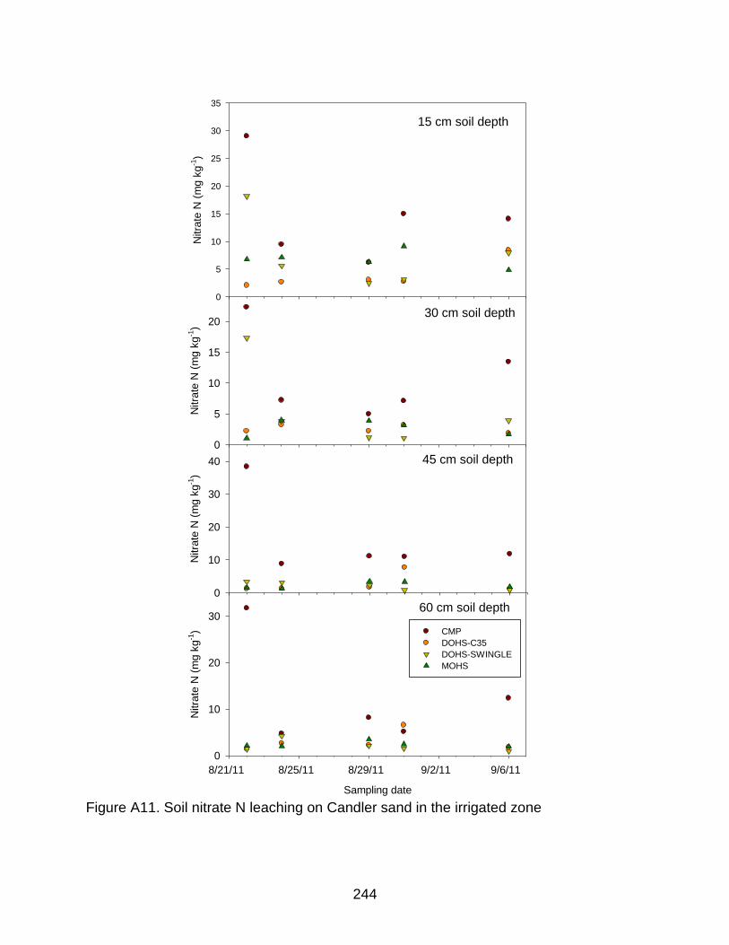
244
60 cm soil depth
Sampling date
8/21/11 8/25/11 8/29/11 9/2/11 9/6/11
Nitra
te N
(m
g k
g-1
)
0
10
20
30
CMP
DOHS-C35
DOHS-SWINGLE
MOHS
45 cm soil depth
Nitra
te N
(m
g k
g-1
)
0
10
20
30
40
30 cm soil depth
Nitra
te N
(m
g k
g-1
)
0
5
10
15
20
15 cm soil depth
Nitra
te N
(m
g k
g-1
)
0
5
10
15
20
25
30
35
Figure A11. Soil nitrate N leaching on Candler sand in the irrigated zone

245
60 cm soil depth
Sampling date
8/21/11 8/25/11 8/29/11 9/2/11 9/6/11
Nitra
te N
(m
g k
g-1
)
0
2
4
6
8
10
12
14
CMP
DOHS-C35
DOHS-SWIGLE
MOHS
45 cm soil depth
Nitra
te N
(m
g k
g-1
)
0
2
4
6
8
30 cm soil depth
Nitra
te N
(m
g k
g-1
)
0
2
4
6
15 cm soil depth
Nitra
te N
(m
g k
g-1
)
0
5
10
15
20
25
30
Figure A12. Soil nitrate N leaching on Candler sand in the nonirrigated zone

246
15 cm soil depth
Mehlic
h 1
P (
mg k
g-1
)
0
50
100
150
200
30 cm soil depth
Mehlic
h 1
P (
mg k
g-1
)
0
20
40
60
80
100
120
45 cm soil depth
Mehlic
h 1
P (
mg k
g-1
)
0
10
20
30
40
60 cm soil depth
Sampling date
6/3/11 6/6/11 6/9/11 6/12/11 6/15/11 6/18/11
Mehlic
h 1
P (
mg k
g-1
)
0
5
10
15
20 CMP
DOHS
MOHS
Figure A13. Soil P leaching on Immokalee sand in the irrigated zone

247
15 cm soil depth
Mehlic
h 1
P (
mg k
g-1
)
0
20
40
60
80
30 cm soil depth
Mehlic
h 1
P (
mg k
g-1
)
0
20
40
60
80
45 cm soil depth
Mehlic
h 1
P (
mg k
g-1
)
0
20
40
60
80
60 cm soil depth
Sampling date
6/3/11 6/6/11 6/9/11 6/12/11 6/15/11 6/18/11
Mehlic
h 1
P (
mg k
g-1
)
0
10
20
30 CMP
DOHS
MOHS
Figure A14. Soil P leaching on Immokalee sand in the nonirrigated zone

248
15 cm soil depth
Mehlic
h 1
P (
mg k
g-1
)
50
100
150
200
250
300
350
30 cm soil depth
Mehlic
h 1
P (
mg k
g-1
)
50
100
150
200
250
300
45 cm soil depth
Mehlic
h 1
P (
mg k
g-1
)
50
100
150
200
250
300
60 cm soil depth
Sampling date
8/21/11 8/25/11 8/29/11 9/2/11 9/6/11
Mehlic
h 1
P (
mg k
g-1
)
50
100
150
200
250
300CMP
DOHS-C35
DOHS-SWINGLE
MOHS
Figure A15. Soil P leaching on Candler sand in the irrigated zone

249
15 cm soil depth
Mehlic
h 1
P (
mg k
g-1
)
50
100
150
200
250
30 cm soil depth
Mehlic
h 1
P (
mg k
g-1
)
50
100
150
200
45 cm soil depth
Mehlic
h 1
P (
mg k
g-1
)
50
100
150
200
60 cm soil depth
Sampling date
8/21/11 8/25/11 8/29/11 9/2/11 9/6/11
Mehlic
h 1
P (
mg k
g-1
)
50
100
150
200
250 CMP
DOHS-C35
DOHS-SWINGLE
MOHS
Figure A16. Soil P leaching on Candler sand in the nonirrigated zone

250
15 cm soil depth
Mehlic
h 1
K (
mg k
g-1
)
0
20
40
60
80
100
30 cm soil depth
Mehlic
h 1
K (
mg k
g-1
)
0
10
20
30
40
50
45 cm soil depth
Mehlic
h 1
K (
mg k
g-1
)
0
20
40
60
60 cm soil depth
Sampling date
6/3/11 6/6/11 6/9/11 6/12/11 6/15/11 6/18/11
Mehlic
h 1
K (
mg k
g-1
)
0
10
20
30
40
CMP
DOHS
MOHS
Figure A17. Soil K leaching on Immokalee sand in the irrigated zone

251
15 cm soil depth
Mehlic
h 1
K (
mg k
g-1
)
0
20
40
60
80
100
120
30 cm soil depth
Mehlic
h 1
K (
mg k
g-1
)
0
20
40
60
80
45 cm soil depth
Mehlic
h 1
K (
mg k
g-1
)
0
10
20
30
40
50
60 cm soil depth
Sampling date
6/3/11 6/6/11 6/9/11 6/12/11 6/15/11 6/18/11
Mehlic
h 1
K (
mg k
g-1
)
0
20
40
60CMP
DOHS
MOHS
Figure A18. Soil K leaching on Immokalee sand in the nonirrigated zone

252
15 cm soil depth
Mehlic
h 1
K (
mg k
g-1
)
0
50
100
150
200
30 cm soil depth
Mehlic
h 1
K (
mg k
g-1
)
0
50
100
150
200
45 cm soil depth
Mehlic
h 1
K (
mg k
g-1
)
0
50
100
150
200
60 cm soil depth
Sampling date
8/21/11 8/25/11 8/29/11 9/2/11 9/6/11
Mehlic
h 1
K (
mg k
g-1
)
0
50
100
150
200CMP
DOHS-C35
DOHS-SWINGLE
MOHS
Figure A19. Soil K leaching on Candler sand in the irrigated zone

253
15 cm soil depth
Mehlic
h 1
K (
mg k
g-1
)
20
40
60
80
100
120
140
30 cm soil depth
Mehlic
h 1
K (
mg k
g-1
)
20
40
60
80
100
120
45 cm soil depth
Mehlic
h 1
K (
mg k
g-1
)
20
40
60
80
100
60 cm soil depth
Sampling date
8/21/2011 8/25/2011 8/29/2011 9/2/2011 9/6/2011
Mehlic
h 1
K (
mg k
g-1
)
20
40
60
80CMP
DOHS-C35
DOHS-SWINGLE
MOHS
Figure A20. Soil K leaching on Candler sand in the nonirrigated zone
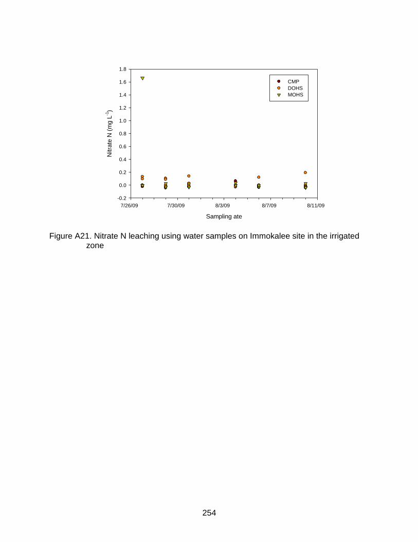
254
Sampling ate
7/26/09 7/30/09 8/3/09 8/7/09 8/11/09
Nitra
te N
(m
g L
-1)
-0.2
0.0
0.2
0.4
0.6
0.8
1.0
1.2
1.4
1.6
1.8
CMP
DOHS
MOHS
Figure A21. Nitrate N leaching using water samples on Immokalee site in the irrigated zone

255
CMP (<0.5 mm)
Cross-row (cm)
0 10 20 30 40
With
in r
ow (
cm)
0
5
10
15
20
25
30
0.10
0.15
0.20
0.25
CMP (d=0-1 mm)
Cross-row (cm)
0 10 20 30 40
With
in r
ow (
cm)
0
5
10
15
20
25
30
0.025
0.030
0.035
0.040
0.045
0.050
0.055
0.060
CMP (d=1-3 mm)
Cross-row (cm)
0 10 20 30 40
With
in r
ow (
cm)
0
5
10
15
20
25
30
0.010
0.015
0.020
0.025
0.030
0.035
0.040
CMP (d>3 mm)
Cross-row (cm)
0 10 20 30 40
With
in r
ow (
cm)
0
5
10
15
20
25
30
0.000
0.002
0.004
0.006
0.008
Figure A22. Lateral RLD distribution at the Immokalee site in June 2009 using CMP in the 0-30 cm soil depth layer. All color scales are in cm cm-3
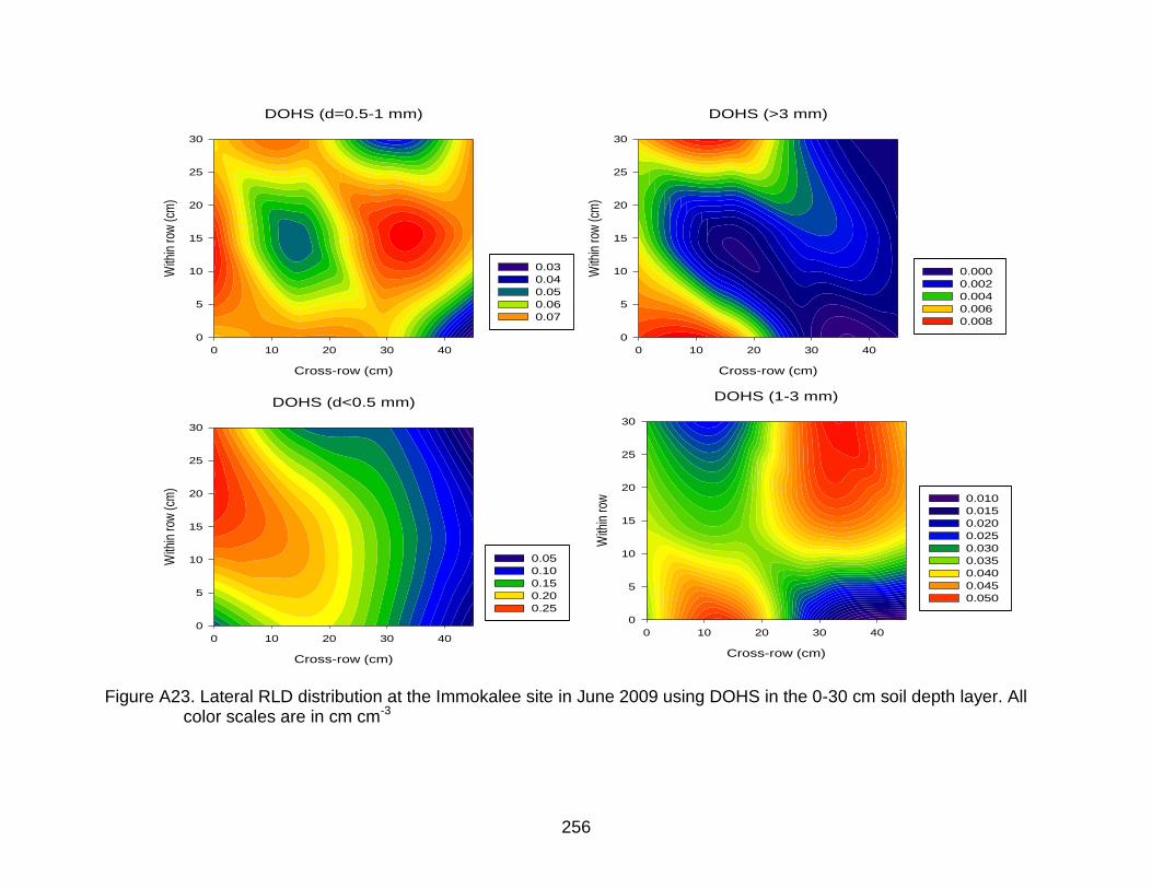
256
DOHS (d<0.5 mm)
Cross-row (cm)
0 10 20 30 40
With
in r
ow (
cm)
0
5
10
15
20
25
30
0.05
0.10
0.15
0.20
0.25
DOHS (d=0.5-1 mm)
Cross-row (cm)
0 10 20 30 40
With
in r
ow (
cm)
0
5
10
15
20
25
30
0.03
0.04
0.05
0.06
0.07
DOHS (1-3 mm)
Cross-row (cm)
0 10 20 30 40
With
in r
ow
0
5
10
15
20
25
30
0.010
0.015
0.020
0.025
0.030
0.035
0.040
0.045
0.050
DOHS (>3 mm)
Cross-row (cm)
0 10 20 30 40
With
in r
ow (
cm)
0
5
10
15
20
25
30
0.000
0.002
0.004
0.006
0.008
Figure A23. Lateral RLD distribution at the Immokalee site in June 2009 using DOHS in the 0-30 cm soil depth layer. All color scales are in cm cm-3

257
MOHS (d<0.5 mm)
Cross-row (cm)
0 10 20 30 40
With
in r
ow (
cm)
0
5
10
15
20
25
30
0.04
0.06
0.08
0.10
0.12
0.14
0.16
0.18
MOHS (d=0.5-1 mm)
Cross-row (cm)
0 10 20 30 40
With
in r
ow (
cm)
0
5
10
15
20
25
30
0.02
0.03
0.04
0.05
0.06
MOHS (d=1-3 mm)
Cross-row (cm)
0 10 20 30 40
With
in r
ow (
cm)
0
5
10
15
20
25
30
0.005
0.010
0.015
0.020
0.025
MOHS (d>3 mm)
Cross-row (cm)
0 10 20 30 40
With
in r
ow (
cm)
0
5
10
15
20
25
30
-0.001
0.000
0.001
0.002
0.003
0.004
0.005
0.006
0.007
Figure A24. Lateral RLD distribution at the Immokalee site in June 2009 using MOHS in the 0-30 cm soil depth layer. All color scales are in cm cm-3

258
CMP (d>3 mm)
Cross-row (cm)
0 10 20 30 40
With
in r
ow
(cm
)
0
5
10
15
20
25
30
0.0005
0.0010
0.0015
0.0020
0.0025
0.0030
0.0035
0.0040
0.0045
CMP (d=1-3 mm)
Cross-row (cm)
0 10 20 30 40
With
in r
ow
(cm
)
0
5
10
15
20
25
30
0.004
0.006
0.008
0.010
0.012
0.014
0.016
0.018
CMP (d=0.5-1 mm)
Cross-row (cm)
0 10 20 30 40
With
in r
ow
(cm
)
0
5
10
15
20
25
30
0.014
0.016
0.018
0.020
0.022
0.024
0.026
0.028
0.030
0.032
CMP (d<0.5 mm)
Cross-row (cm)
0 10 20 30 40
With
in r
ow
(cm
)
0
5
10
15
20
25
30
0.07
0.08
0.09
0.10
0.11
Figure A25. Lateral RLD distribution at the Immokalee site in June 2010 using CMP in the 0-45 cm soil depth layer. All color scales are in cm cm-3

259
DOHS (>3 mm)
Cross-row (cm)
0 10 20 30 40
With
in r
ow
(cm
)
0
5
10
15
20
25
30
0.002
0.004
0.006
0.008
0.010
DOHS (d=1-3 mm)
Cross-row (cm)
0 10 20 30 40
With
in r
ow
(cm
)
0
5
10
15
20
25
30
0.020
0.025
0.030
0.035
0.040
0.045
DOHS (d=0.5-1 mm)
Cross-row (cm)
0 10 20 30 40
With
in r
ow
(cm
)
0
5
10
15
20
25
30
0.035
0.040
0.045
0.050
0.055
DOHS (d<0.5 mm)
Cross-row (cm)
0 10 20 30 40
With
in r
ow
(cm
)
0
5
10
15
20
25
30
0.15
0.20
0.25
0.30
Figure A26. Lateral RLD distribution at the Immokalee site in June 2010 using DOHS in the 0-45 cm soil depth layer. All color scales are in cm cm-3

260
MOHS (d>3mm)
Cross-row (cm)
0 10 20 30 40
With
in r
ow
(cm
)
0
5
10
15
20
25
30
0.002
0.004
0.006
0.008
0.010
MOHS (d=1-3 mm)
Cross-row (cm)
0 10 20 30 40
With
in r
ow
(cm
)
0
5
10
15
20
25
30
0.006
0.008
0.010
0.012
0.014
0.016
0.018
0.020
0.022
MOHS (d=0.5-1 mm)
Cross-row (cm)
0 10 20 30 40
With
in r
ow
(cm
)
0
5
10
15
20
25
30
0.015
0.020
0.025
0.030
0.035
MOHS (d<0.5 mm)
Cross-row (cm)
0 10 20 30 40
With
in r
ow
(cm
)
0
5
10
15
20
25
30
0.08
0.10
0.12
0.14
0.16
0.18
0.20
0.22
0.24
Figure A27. Lateral RLD distribution at the Immokalee site in June 2010 using MOHS in the 0-45 cm soil depth layer. All color scales are in cm cm-3

261
Root diameter (mm)
<0.5mm 0.5-1mm 1-3mm >3mm
Root
length
densi
ty (
cm/c
m3)
0.0
0.2
0.4
0.6
0.8
1.0
DOHS-Swingle
Figure A28. Lateral RLD distribution as a function of irrigation method at the Lake Alfred site in December 2009 using DOHS-Swingle. Error bars denote one standard deviation

262
Root diameter (mm)
<0.5mm 0.5-1mm 1-3mm >3mm
Root le
ngth
densi
ty (
cm c
m-3
)
0.0
0.2
0.4
0.6
0.8
1.0
DOHS-C35
Figure A29. Lateral RLD distribution as a function of irrigation method at the Lake Alfred site in December 2009 using DOHS-C35. Error bars denote one standard deviation

263
Root diameter (mm)
<0.5mm 0.5-1mm 1-3mm >3mm
Root
length
density
(cm
cm
-3)
0.0
0.1
0.2
0.3
0.4
CMP
Figure A30. Lateral RLD distribution as a function of irrigation method at the Lake Alfred site in December 2009 using CMP. Error bars denote one standard deviation

264
Root diameter (mm)
<0.5mm 0.5-1mm 1-3mm >3mm
Roo
t len
gth
dens
ity (
cm c
m-3
)
0.0
0.1
0.2
0.3
0.4
0.5
MOHS
Figure A31. Lateral RLD distribution as a function of irrigation method at the Lake Alfred site in December 2009 using MOHS. Error bars denote one standard deviation

265
CMP (d<0.5 mm)
Cross-row (cm)
0 5 10 15 20 25 30
With
in ro
w (c
m)
0
5
10
15
20
25
30
0.08
0.10
0.12
0.14
0.16
0.18
0.20
0.22
CMP (d=0.5-1 mm)
Cross-row (cm)
0 5 10 15 20 25 30
With
in ro
w (c
m)
0
5
10
15
20
25
30
0.010
0.015
0.020
0.025
0.030
0.035
0.040
0.045
0.050
CMP (d=1-3 mm)
Cross-row (cm)
0 5 10 15 20 25 30
With
in ro
w (c
m)
0
5
10
15
20
25
30
0.010
0.015
0.020
0.025
CMP (d>3 mm)
Cross-row (cm)
0 5 10 15 20 25 30
With
in ro
w (c
m)
0
5
10
15
20
25
30
1e-3
2e-3
3e-3
4e-3
5e-3
6e-3
Figure A32. Lateral RLD distribution as a function of irrigation method at the Lake Alfred site in July 2010 using CMP. The color scale is in cm cm-3

266
DOHS-SWINGLE (d<0.5 mm)
Cross-row (cm)
0 5 10 15 20 25 30
With
in r
ow (
cm)
0
5
10
15
20
25
30
0.3
0.4
0.5
0.6
0.7
0.8
0.9
1.0
DOHS-SWINGLE (0.5-1 mm)
Cross-row (cm)
0 5 10 15 20 25 30
With
in r
ow (
cm)
0
5
10
15
20
25
30
0.015
0.020
0.025
0.030
0.035
0.040
0.045
DOHS-SWINGLE (1-3 mm)
Cross-row (cm)
0 5 10 15 20 25 30
With
in r
ow (
cm)
0
5
10
15
20
25
30
0.015
0.020
0.025
0.030
0.035
0.040
0.045
0.050
0.055
DOHS-SWINGLE (>3 mm)
Cross-row (cm)
0 5 10 15 20 25 30
With
in r
ow (
cm)
0
5
10
15
20
25
30
0.000
0.002
0.004
0.006
0.008
0.010
0.012
Figure A33. Lateral RLD distribution as a function of irrigation method at the Lake Alfred site in July 2010 using DOHS-Swingle. The color scale is in cm cm-3

267
DOHS-C35 (d<0.5 mm)
Cross-row (cm)
0 5 10 15 20 25 30
With
in ro
w (c
m)
0
5
10
15
20
25
30
0.4
0.6
0.8
1.0
DOHS-C35 (d=0.5-1 mm)
Cross-row (cm)
0 5 10 15 20 25 30
With
in ro
w (c
m)
0
5
10
15
20
25
30
0.005
0.010
0.015
0.020
0.025
0.030
DOHS-C35 (d=1-3 mm)
Cross-row (cm)
0 5 10 15 20 25 30
With
in ro
w (c
m)
0
5
10
15
20
25
30
0.005
0.010
0.015
0.020
0.025
0.030
DOHS-C35 (>3 mm)
Cross-row (cm)
0 5 10 15 20 25 30
With
in ro
w (c
m)
0
5
10
15
20
25
30
0.001
0.002
0.003
0.004
0.005
0.006
0.007
Figure A34. Lateral RLD distribution as a function of irrigation method at the Lake Alfred site in July 2010 using DOHS-C35. The color scale is in cm cm-3

268
MOHS (d<0.5 mm)
Cross-row (cm)
0 5 10 15 20 25 30
With
in ro
w (c
m)
0
5
10
15
20
25
30
0.20
0.25
0.30
0.35
0.40
0.45
0.50
0.55
MOHS (d=0.5-1 mm)
Cross-row (cm)
0 5 10 15 20 25 30
With
in ro
w (c
m)
0
5
10
15
20
25
30
0.015
0.020
0.025
0.030
0.035
MOHS (d=1-3 mm)
Cross-row (cm)
0 5 10 15 20 25 30
With
in ro
w (c
m)
0
5
10
15
20
25
30
0.014
0.016
0.018
0.020
0.022
0.024
0.026
0.028
0.030
MOHS (d>3 mm)
Cross-row (cm)
0 5 10 15 20 25 30
With
in ro
w (c
m)
0
5
10
15
20
25
30
0
1e-3
2e-3
3e-3
4e-3
5e-3
6e-3
7e-3
8e-3
Figure A35. Lateral RLD distribution as a function of irrigation method at the Lake Alfred site in July 2010 using MOHS. The color scale is in cm cm-3

269
190 195 200 205 210
Sap f
low
per
unit land a
rea (
mm
d-1
)
0.0
0.1
0.2
0.3
0.4
DOHS-Swingle
CMP
Julian Day
Figure A36. Average sap flow per unit land area at Lake Alfred site in July 2010. Error bars denote one standard deviation
70 72 74 76 78 80 82 84
0.0
0.2
0.4
0.6
0.8
1.0
1.2
1.4
1.6
DOHS-SWINGLE
CMP
MOHS
DOHS-C35
Sa
p f
low
per
un
it la
nd a
rea
(m
m d
-1)
Julian Day
Figure A37. Average sap flow per unit land area at Lake Alfred site in March 2011. Error bars denote one standard deviation

270
Julian day
46 48 50 52 54 56 58 60 62
Sap f
low
(m
m d
-1)
-0.5
0.0
0.5
1.0
1.5
2.0
2.5
3.0
3.5
DOHS
Figure A38. Average sap flow per unit land area at Immokalee in March 2011. Error bars denote one standard deviation

271
Julian day
152 154 156 158 160 162 164 166 168 170 172 174
Sap f
low
(m
m d
-1)
0
1
2
3
4
5
6
DOHS
MOHS
CMP
Figure A39. Average sap flow per unit land area at Immokalee in June 2011. Error bars
denote one standard deviation
234 236 238 240 242 244 246 248 250 252
0
2
4
6
DOHS-SWINGLE
CMP
MOHS
DOHS-C-35
Sap
flo
w p
er
un
it l
an
d a
rea (
mm
d-1
)
Julian Day
Figure A40. Average sap flow per unit land area at Lake Alfred site in August-September 2011. Error bars denote one standard deviation

272
Julian day
190 195 200 205 210
Cum
ula
tive s
ap f
low
(m
m)
0
1
2
3
4
5
DOHS
CMP
Figure A41. Cumulative sap flow at Lake Alfred site in July 2010. Error bars denote one
standard deviation
Julian day
68 70 72 74 76 78 80 82 84
Cum
ula
tive s
ap f
low
(m
m)
0
2
4
6
8
10
DOHS-SWINGLE
CMP
MOHS
DOHS-C35
Figure A42. Cumulative sap flow at Lake Alfred site in March 2011. Error bars denote
one standard deviation

273
Julian day
234 236 238 240 242 244 246 248 250 252
Cum
ulat
ive
sapf
low
(mm
)
0
10
20
30
40
50
60
DOHS-Swingle
CMP
MOHS
DOHS-C35
Figure A43. Cumulative sap flow at Lake Alfred site in August-September 2011. Error
bars denote one standard deviation
Julian day
46 48 50 52 54 56 58 60 62
Cu
mu
lativ
e s
ap f
low
(m
m)
0
2
4
6
8
10
12
14
16
18
DOHS
Figure A44. Cumulative sap flow at Immokalee site in February-March 2011. Error bars denote one standard deviation

274
Julian day
152 154 156 158 160 162 164 166 168 170 172 174
Cum
ulat
ive
sap
flow
(m
m)
0
10
20
30
40
50
60
70
DOHS
MOHS
CMP
Figure A45. Cumulative sap flow at Immokalee site in June 2011. Error bars denote
one standard deviation
190 195 200 205 210
0.00
0.02
0.04
0.06
0.08
0.10
DOHS-SWINGLE
CMP
Index s
apflow
coeff
icie
nt,
Kc
Julian Day Figure A46. Average index sap flow Kc at the Lake Alfred site in July 2010. Error bars
denote one standard deviation

275
68 70 72 74 76 78 80 82 84
0.0
0.1
0.2
0.3
0.4
DOHS-SWINGLE
CMP
MOHS
DOHS-C35
Inde
x sa
pflo
w c
oeffi
cien
t, K
c
Julian Day Figure A47. Average index sap flow Kc at the Lake Alfred site in March 2011. Error bars
denote one standard deviation

276
Julian Day234 236 238 240 242 244 246 248 250 252
0.0
0.5
1.0
1.5
2.0
2.5
DOHS-SWINGLE
CMP
MOHS
DOHS-C35
Inde
x sa
pflo
w c
oeffi
cien
t, K c
Figure A48. Average index sap flow Kc at the Lake Alfred site in August-September
2011. Error bars denote one standard deviation
Julian day
46 48 50 52 54 56 58 60 62
Index s
ap f
low
Kc
0.1
0.2
0.3
0.4
0.5
0.6
DOHS
Figure A49. Average index sap flow Kc at the Immokalee site in February-March 2011.
Error bars denote one standard deviation

277
Julian day
152 154 156 158 160 162 164 166 168 170 172 174
Inde
x sa
pflo
w (
Kc )
0.0
0.2
0.4
0.6
0.8
1.0
DOHS
MOHS
CMP
Figure A50. Average index sap flow Kc at the Immokalee site in June 2011. Error bars
denote one standard deviation

278
APPENDIX B CHARACTERIZATION OF SORPTION ISOTHERMS FOR AMMONIUM-N, K AND P
ON THE FLATWOODS AND RIDGE SOILS
The chemical characteristics of soils dominating the Flatwoods and Ridge regions
of Florida are well described in Obreza and Collins (2008) and some were also
determined in this study. The Immokalee and Candler fine sand are moderately acidic
(pH ranging from 4.9 to 5.6), have low organic matter content (ranging from 0.41 to
0.61% on Immokalee fine sand and from 1.56 to 1.96% on Candler fine sand) and low
cation exchange capacity (CEC) (ranging from 2 to 6 cmol (+) kg-1), have inorganic N in
the range of 8.20 and 11.24 mg kg-1, moderate to very high P (in the range of 28.73-
46.45 mg kg-1 for Immokalee sand and 112.79-115.82 mg kg-1 for Candler fine sand)
and K in the range of 11.83-15.23 mg kg-1 for Immokalee fine sand and 23.03-29.70 mg
kg-1 for Candler fine sand (Table B1). The study speculates that the properties such as
organic matter content and CEC are behind the adsorption processes of the nutrients in
this study.
Adsorption is the mechanism most commonly responsible for the retention of
solutes by soils, particularly cations and phosphorus. The sorption process tends to
restrict compound’s mobility and bioavailability (Essington, 2004). Thus, the procedure
for determining the NH4-N, P and K sorption isotherms could then provide information
on their mobility in the soil. The supporting electrolyte concentration is chosen to mimic
that of soil solution. Most commonly 0.01 M CaCl2 (Singh and Jones, 1975; Belmont et
al., 2009), 0.01 N CaCl2 (Bowman et al., 1981), 0.005 M CaCl2 (Essington, 2004), 5-100
mg K L-1 KCl (Sparks et al., 1980), 0.05 M KCl (Harris et al., 1996; Zhou and Li, 2001),
and 0.01 M KCl (Nair et al., 1998; Villapando and Graetz, 2001) have been used as
electrolytes in studies on P and K sorption. Nair et al. (1984) reported that P sorption

279
varies with ionic strength and cation species of the supporting electrolyte. For example,
Nair et al. (1984) showed that P adsorption was generally lower with K+ as the
supporting electrolyte cation compared with Ca2+. These studies and others have not
explained the rationale behind use of a particular electrolyte other than equilibrating the
solutions in deionized or tap water. This study attempted to 1) determine sorption
isotherms for NH4+, K and P on the Flatwoods and Ridge soils with the aim of predicting
the mobility, availability and uptake of NH4+, P and K in citrus production, and 2)
determine the effect of supporting electrolyte on P sorption. We hypothesized that P
adsorption and NH4+ and K+ exchange on the Flatwoods and Ridge soils do not
adversely affect availability and uptake as a result of adsorption to soil colloids.
Results and Discussion
The results of adsorption of K+, NH4+-N, and P are presented and described in Fig.
B1 through B3, Tables B2 and B3, and Appendices G through I for Candler and
Immokalee fine sand. Ammonium adsorption for Immokalee and Candler fine sand
followed a linear isotherm with distribution coefficients (KD) of 1.12±0.42 and 1.64±0.25
kg L-1 and 1.66±0.39 and 1.76±0.39 kg L-1 for the 0-15- and 15-30 cm depths,
respectively. P adsorption was described by a Freundlich model with linearized KD
ranging from 0.50±0.19 to 0.75±0.13 kg L-1 for Immokalee fine sand and from 1.73±0.15
to 4.43±0.50 kg L-1 for Candler fine sand using a Cmax of 15 mg L-1. P sorption isotherm
for Immokalee fine sand determined using fertilizer mixture was linear with KD averaging
about 0.44±10 kg L-1.
The adsorption of K+ and NH4+ was similar for both 0-15- and 15-30 cm soil depth
layers while P adsorption was linear for the P concentration range studied on the
Immokalee sand using fertilizer mixture. Ammonium KD was higher than that of

280
potassium probably due to a larger hydrated radius in the former (ammonium ionic
radius =0.56 nm and potassium ionic radius =0.53 nm). In other words more NH4+ would
be retained in the limited exchange sites of the colloidal fractions (due low organic
matter content ~1-2%, and a small clay fraction ~0.5% (Obreza and Collins, 2008) while
letting K+ desorb into the soil solution for plant uptake. Lumbanraja and Evangelou
(1990; 1994) also reported similar phenomena regarding K+ and NH4+-N on clay loam
and silt loams soils of Kentucky, USA. They showed that the addition of K+ stimulated
the adsorption of NH4+-N on high affinity sites while K+ adsorption was suppressed by
labile NH4+. In a later study done in Florida’s Spodosol and Entisol, Wang and Alva
(2000) showed that NH4+ adsorption was greater for surface soils than that of the
subsurface soils. They found that the potential NH4+ buffering capacity was greater for
Wabasso (at 0-30 and 60-90 cm) than the Candler soil (0-60cm) owing to the presence
of smectite in the former. Studies regarding ammonia sorption done over the years
have yielded mixed observations. For example, Wagenet et al. (1977) assumed
reversible, linear equilibrium sorption with distribution coefficients between 1 and 10 L
kg-1 on a Tyndall silty loam. Yet, Rodríguez et al. (2005) found that representing
ammonium adsorption-desorption as a kinetic process better described their results.
They noted that ammonium adsorption on the sandy clay loam soil was higher than
adsorption on the loamy sand. The ammonium KD values found in this study agree with
those proposed by several researchers (Wagenet et al., 1977; Selim and Iskandar,
1981; Lotse et al., 1992; Ling and El-Kadi, 1998).
Khakural and Alva (1996) studied transformation of urea and ammonium nitrate in
an Entisol and a Spodosol under citrus production. The percentage of transformation of

281
NH4+-N into NO3
--N was 33 to 41 and 37 to 41% in the Candler fine sand and Wabasso
sand, respectively, at application rates of 1 g N kg-1. The rate of transformation of NH4
in these sandy soils dictates the availability of NH4+-N and NO3
--N forms of N for plant
uptake and losses due to volatilization, leaching, and denitrification. We had speculated
that some NH4+ would volatilize and transform into NO3
- but 24 h equilibration time,
under laboratory conditions at 25±1 oC renders this volatilization negligible while
retaining the possible transformation due to nitrification.
Freundlich sorption coefficients (Kf) (Appendix I) were lower for Immokalee fine
sand than for Candler. High coefficients observed on Candler fine sand with Kf eightfold
greater than that of Immokalee fine sand. The Kf value obtained with 0.005 M CaCl2
was approximately twice that obtained with 0.01 M KCl and threefold that obtained in
the fertilizer mixture suggesting the influence of the cation effect on P adsorption than
with water. According to Zhou and Li (2001), the lower Freundlich sorption coefficients
(Kf), indicate low P retention capacity at low P concentrations suggesting that the
potential risk of subsurface P movement and leaching would be high when the
concentration of P in surface soils is high. The Kf and KD values reported in Appendix I
are generally lower than those reported for carbonatic soils in south Florida (Zhou and
Li, 2001) where KD ranged from 14.8 – 76.3 L kg-1 and Kf from 12-58 mg1-N kg-1 LN.
However, the results in this study agree with those of other researchers (Barrow et al.,
1980; Nair et al., 1984; Havlin et al., 2005). According to Havlin et al. (2005), divalent
cations on the CEC enhance P adsorption relative to monovalent cations because they
increase the accessibility of (+)–charged edges of clay minerals to P. This occurs at
pH<6.5, because at greater soil pH Ca-P minerals would precipitate. Barrow et al.

282
(1980) also showed that at equal ionic strength below pH=6, there was more phosphate
adsorption from CaCl2 than from NaCl on goethite. This phenomenon, according to
Barrow and colleagues, is caused because high concentration of positive charges near
the negatively charged soil surface may be induced by replacing a monovalent cation
with a divalent one and also if the added divalent cation has a specific affinity for the
adsorption surface. Addition of cations from the supporting electrolyte, unlike using the
fertilizer, induced a greater negative charge for phosphate adsorption. The higher
sorption coefficients for Candler might be due to high organic matter and some Fe/Al
coatings that might bind P. This might explain, in part, why Mehlich 1 P was several
times higher for Candler than for Immokalee fine sand as summarized in Table B1 and
discussed thoroughly in Chapter 3. The high Kf value in the top 0-15 cm than the 15-30
cm layer is ascribed to higher organic carbon and organic matter in the former layer
resulting in increased P adsorption.
Summary
The results show that P adsorption in the top 0-15 cm was greater for Candler
than Immokalee sand using the fertilizer mixture, 0.005 M CaCl2 and 0.01 M KCl. The
distribution coefficients (KD) for P estimated using 0.01 M KCl were similar to KD values
determined using fertilizer mixture for Immokalee and Candler fine sand, respectively.
The KD values determined using 0.005 M CaCl2 as the supporting electrolyte were two-
to threefold greater than the KD of the fertilizer mixture on Immokalee and Candler fine
sand suggesting that divalent Ca+2 might result in overestimation of P sorption on
Candler and Immokalee sandy soils. It appears the addition of a supporting electrolyte
with a divalent or monovalent cation, unlike fertilizer mixture, increases the surface
charge for adsorption of orthophosphate anions. The adsorption isotherms of both

283
ammonium and potassium were linear and greater for Candler than Immokalee sand
probably due to Al and Fe coatings and higher organic matter in the former. For the two
soils soils, ammonium adsorption coefficients were greater than those of potassium.

284
Table B1. Selected soil chemical characteristics for Immokalee and Candler sand
Soil Soil depth (cm)
pH¶ OM§ CEC‡ NH4+ NO3
- M1P† M1K‡‡ IN¶¶
Immokalee 0-15 5.6 0.61 2-6 3.45 4.93 46.45 15.23 8.37 Immokalee 15-30 5.2 0.41 2-6 2.32 4.07 28.73 11.83 6.40 Candler 0-15 5.3 1.96 2-4 2.55 8.69 115.82 29.70 11.24 Candler 15-30 4.9 1.56 2-4 2.88 5.31 112.79 23.03 8.20 ¶Soil to water ratio=1:2 (mass/volume), §OM-organic matter expressed as a percentage, ‡CEC-cation exchange capacity expressed in cmol(+) kg-1 (CEC reported by Obreza and Collins, 2008), †Mehlich 1 P (mg kg-1), ‡‡Mehlich 1 K (mg kg-1), ¶¶IN=Inorganic N (mg kg-1)

285
Table B2. Sorption coefficients for NH4+ and K+ on Immokalee and Candler fine sand
using fertilizer mixture in tap water
Soil Depth (cm) NH4+ K+
¶KD (L kg-1) KD (L kg-1)
Immokalee 0-15 1.12±0.42 0.91±0.38
Immokalee 15-30 1.64±0.25 0.87±0.74
Candler 0-15 1.66±0.39 1.65±0.56
Candler 15-30 1.76±0.39 0.93±0.28 ¶KD =Mean±one standard deviation of 3 replications
Table B3. Sorption coefficients for P on Immokalee and Candler fine sand
Soil Depth (cm) Supporting electrolyte ‡KD (L kg-1)
Immokalee 0-15 0.01 M KCl 0.53 ± 0.11
Immokalee 15-30 0.01 M KCl 0.50 ± 0.19
Candler 0-15 0.01 M KCl 2.87 ± 0.43
Candler 15-30 0.01 M KCl 3.79 ± 0.87
Immokalee 0-15 0.005 M CaCl2 0.75 ± 0.13
Immokalee 15-30 0.005 M CaCl2 0.74 ± 0.32
Candler 0-15 0.005 M CaCl2 3.46 ± 0.65
Candler 15-30 0.005 M CaCl2 4.43 ± 0.50
Immokalee 0-15 Fertilizer mixture 0.45 ± 0.10
Immokalee 15-30 Fertilizer mixture 0.43 ± 0.20
Candler 0-15 Fertilizer mixture 1.73 ± 0.15
Candler 15-30 Fertilizer mixture 2.05 ± 0.89 ‡KD=Linearized KD using Equation 6-6 presented as mean±one standard deviation of 3 replications and a Cmax of 15 mg L-1

286
Candler sand 0-15 cm
Se=2.04Ce, R2=0.9808
Solution NH4 (mg/L)
0 10 20 30 40 50
Aso
rbed
NH
4 c
on
cen
trati
on
(m
g/k
g)
0
20
40
60
80
Candler sand 15-30 cm
Se=2.20Ce, R2=0.9945
0 10 20 30 40 50
0
20
40
60
80
Immokalee sand 0-15 cm
Se = 1.00Ce, R
2=0.9817
0
10
20
30
40
50
60
Immokalee sand 15-30 cm
Se = 1.35Ce, R2=0.9849
0
10
20
30
40
50
60
Figure B1. Selected linear isotherms for NH4
+ for Immokalee and Candler sand

287
Candler sand 15-30 cm
S=33.39C0.28
, KD=2.09,
R2=0.9634
Solution P concentration (mg/L)
0 5 10 15 20 25 30
0
20
40
60
80
Candler sand 0-15 cm
S=29.85C0.21
, KD
= 1.43,
R2
=0.9671
Ad
so
rbe
d c
on
cen
trati
on
(m
g/k
g)
0
20
40
60
80
Immokalee 0-15 cm
S=2.18C0.54
, KD= 0.76,
R2=0.9585
0
5
10
15
20
25
30
Immokalee sand 15-30 cm
S=3.97C0.51
,KD=1.28,
R
2=0.9492
0 10 20 30 40 50
0
10
20
30
Figure B2. Selected Freundlich isotherms for P for Immokalee and Candler sand using 0.005M CaCl2

288
Candler sand 15-30 cm
S=19.33C0.48, KD=2.61,
R2=0.9837
0 5 10 15 20 25
0
20
40
60
80
Immokalee 0-15 cm
Se=0.14Ce, R2=0.9773
Ad
so
rbed
co
ncen
trati
on
(m
g/k
g)
0
2
4
6
8
10
12
14
16
18
Candler sand 0-15 cm
S=9.01C0.61, KD=2.01,
R2=0.98790
10
20
30
40
50
60
70
Immokalee 15-30 cm
S=2.79C0.49, KD=0.86,
R2=0.9932
Solution concentration (mg/L)
0 10 20 30 40 50
0
5
10
15
20
Figure B3. Selected linear and Freundlich isotherms for P for Immokalee and Candler sand using 0.01M KCl

289
APPENDIX C SOIL WATER CHARACTERISTIC CURVE AND HYDRAULIC FUNCTIONS FOR THE
IMMOKALEE AND CANDLER SAND
The soil properties that determine the behavior of soil water flow systems are the
hydraulic conductivity and water retention characteristics. The relation between soil
water content and the soil water suction is a fundamental part of the characterization of
the hydraulic properties of soil (Klute, 1986). The conductivity of a soil depends on pore
geometry and the properties of the fluid flowing through or retained in the pores.
Viscosity and density are the two properties that directly affect hydraulic conductivity
while soil porosity and water retention function are determined by soil texture and
structure (Klute and Dirksen, 1986). The hydraulic conductivity is defined by Darcy’s
Law (Klute and Dirksen, 1986; Hillel, 1998) which for one-dimensional vertical flow may
be written as:
( )
(C-1)
where q is the volume flux density,
is the gradient of the hydraulic head H, and
K(θ) is the hydraulic conductivity. The driving force is expressed as the negative
gradient of the hydraulic head composed of the gravitational head, z, and the pressure
head, h, mathematically given as:
H=h+z (C-2)
Mualem (1986) also explained that there are some independent variables of
interest that describe soil water retention characteristics such as the degree of
saturation (S), effective water content ( ), effective saturation could also be used to
describe water retention characteristics.

290
The amount of water retained in the soil at any given moment is dependent upon
factors such as the type of plant cover, plant density, stage of plant growth, rooting
depth, evaporation and transpiration rates, amount of water infiltrated, rate of wetting,
nature of horizonation and the length of time since the last irrigation or rainfall event
(Cassel and Nielsen, 1986). Amount of water available for plant use is determined
through estimation of available water capacity, field capacity and permanent wilting
point. The traditional field capacity for well-drained sandy soil under laboratory
conditions is estimated at 10 kPa of soil water tension for a sandy soil and 33 kPa for
medium or fine-textured soil (Obreza et al., 1997). However, in their study on soil
water-holding characteristic on Florida Flatwoods and Ridge soils, Obreza and co-
workers showed that soil water tension of 5 kPa would be appropriate for the Ridge and
8 kPa for the Flatwoods soil due to their inherent differences in porosity, conductivity
and horizonation.
Thus, the objectives of the laboratory experiments were to 1) determine water
retention characteristics for the Immokalee and Candler sand and 2) calculate hydraulic
parameters for use in HYDRUS model. We hypothesized basing on literature and field
observations that the soil water retention characteristics for the two sites would vary as
a function of soil depth. Thus, it would be important to sample by depths of interest at
each study site for use of selected site-specific parameters in the simulation model.
Results and Discussion
The volumetric moisture contents at soil tensions ranging from 0-100 kPa (0-1020
cm) are presented in Fig. C1and C2. The Van Genuchten model water retention
parameters (α, n and l) are documented in Table C1. The saturated and residual
moisture contents, moisture contents at field capacity (10 kPa), available soil water

291
content, saturated hydraulic conductivity and bulk density are presented in Table C2.
The residual moisture contents from literature are 0.013 and 0.009 cm3 cm-3 for
Immokalee and Candler fine sand (Carlisle et al., 1989). The saturated hydraulic
conductivity ranged from 13.22 to 15.82 cm h-1 on Immokalee and 14.76 to 15.94 cm h-1
on Candler fine sand. Field capacities averaged 0.096 and 0.093 cm3 cm-3 for the two
soils. Available water capacities ranged from 0.077 to 0.087 and 0.065 to 0.095 cm3
cm-3 for Immokalee and Candler fine sand. The available water capacities were
estimated using soil tensions of 10 kPa as field capacity and 1500 kPa as wilting point.
The results suggested very high hydraulic conductivities, good drainage and
permeability for both soils due to the strong sandy soil characteristic in the top 0.60 m
soil depth. The soil desorption curves also indicate large soil pore sizes and a narrow
pore-size distribution in both soils (Klute, 1986; Klute and Dirksen, 1986; Obreza et al.,
1997; Obreza and Pitts, 2002). The high hydraulic conductivity values suggest the
importance of careful water and nutrient management due to the potential threat of
nutrient leaching and downward drainage of water beyond the plant root zone.
Summary
The soil the hydraulic conductivity and water retention characteristics are
important for better nutrient and water management particularly in fertigated and
irrigated systems. The experiment yielded important site-specific parameters like alpha,
n, m, field capacity, available water capacity and hydraulic conductivity for use in the
HYDRUS-2D model to describe water and solute transport to aid decision-making in
predicting environmental fate of fertilizers.
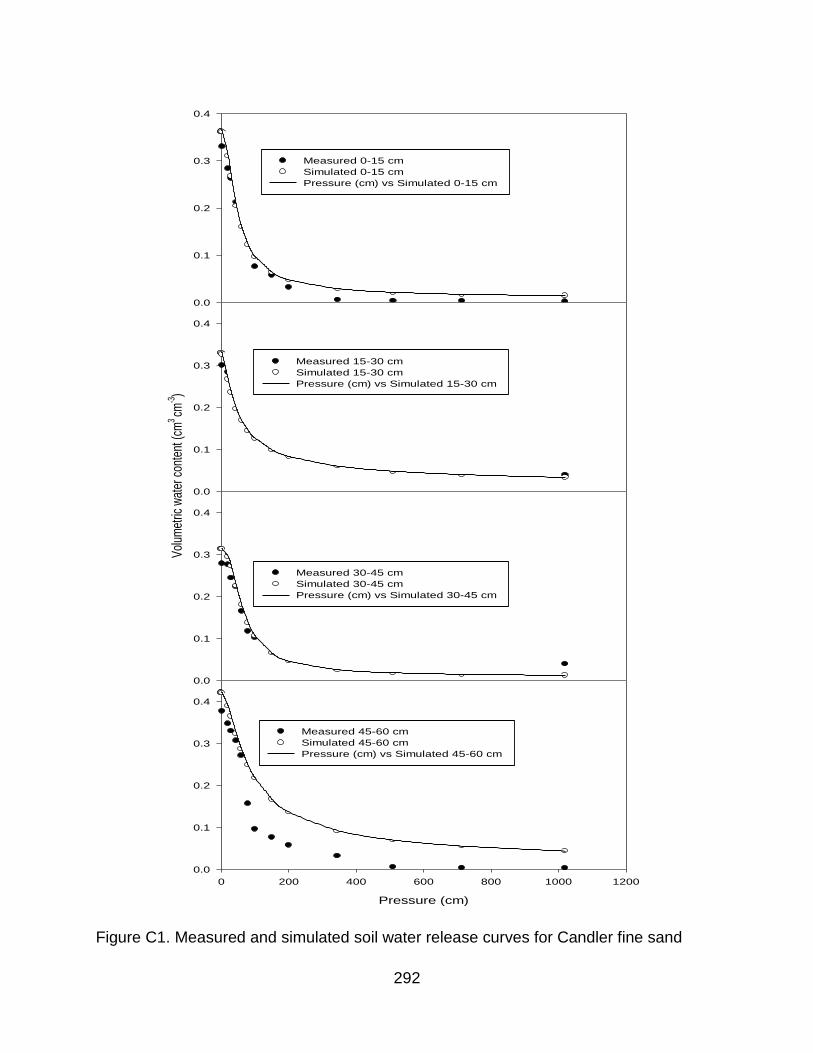
292
0.0
0.1
0.2
0.3
0.4
Measured 0-15 cm
Simulated 0-15 cm
Pressure (cm) vs Simulated 0-15 cm V
olum
etric
wat
er c
onte
nt (c
m3 cm
-3)
0.0
0.1
0.2
0.3
0.4
Measured 15-30 cm
Simulated 15-30 cm
Pressure (cm) vs Simulated 15-30 cm
0.0
0.1
0.2
0.3
0.4
Measured 30-45 cm
Simulated 30-45 cm
Pressure (cm) vs Simulated 30-45 cm
Pressure (cm)
0 200 400 600 800 1000 1200
0.0
0.1
0.2
0.3
0.4
Measured 45-60 cm
Simulated 45-60 cm
Pressure (cm) vs Simulated 45-60 cm
Figure C1. Measured and simulated soil water release curves for Candler fine sand

293
0.0
0.1
0.2
0.3
0.4
Measured 0-15 cm
Simulated 0-15 cm
Simulated 0-15 cm
Volu
met
ric w
ater
con
tent
(cm
3 cm
-3)
0.0
0.1
0.2
0.3
0.4
Measured 15-30 cm
Simulated 15-30 cm
Simulated 15-30 cm
0.0
0.1
0.2
0.3
0.4
Measured 30-45 cm
Simulated 30-45 cm
Simulated 30-45 cm
Pressure (cm)
0 200 400 600 800 1000 1200
0.0
0.1
0.2
0.3
0.4
Measured 45-60 cm
Simulated 45-60 cm
Simulated 45-60 cm
Figure C2. Measured and simulated soil water release curves for Immokalee fine sand

294
Table C1. Soil water retention parameters of Immokalee and Candler fine sand estimated using CAS software developed by Bloom (2009)
Soil Depth (cm) α (cm-1) n m ¶l
Immokalee 0-15 0.03 1.87 0.47 0.5
Immokalee 15-30 0.04 1.29 0.23 0.5
Immokalee 30-45 0.03 2.06 0.52 0.5
Immokalee 45-60 0.03 1.71 0.42 0.5
Candler 0-15 0.03 2.22 0.55 0.5
Candler 15-30 0.04 1.70 0.41 0.5
Candler 30-45 0.02 2.50 0.60 0.5
Candler 45-60 0.02 1.82 0.45 0.5 ¶Pore connectivity parameter (estimated to be an average of 0.5 for many soils)
(Simunek et al., 2007)

295
Table C2. Soil physical characteristics of the Immokalee and Candler fine sand
Soil Depth (cm) Bulk
density (g cm-3)
‡‡Ksat (cm h-1) §θsat (cm3 cm-3) §§θr (cm3 cm-3) ‡FC (cm3
cm-3)
†AWC (cm3 cm-3)
Immokalee 0-15 1.62 15.82 0.343 0.013 0.090 0.077
Immokalee 15-30 1.62 13.97 0.362 0.013 0.100 0.087
Immokalee 30-45 1.59 13.22 0.390 0.013 0.100 0.087
Immokalee 45-60 1.61 14.57 0.318 0.013 0.095 0.082
Candler 0-15 1.65 15.53 0.362 0.009 0.074 0.065
Candler 15-30 1.64 15.94 0.330 0.009 0.104 0.095
Candler 30-45 1.57 14.76 0.313 0.009 0.100 0.091
Candler 45-60 1.68 15.73 0.421 0.009 0.094 0.085 ‡‡Ksat – Saturated hydraulic conductivity
§θsat – Saturated moisture content §§θr – Residual moisture content obtained from Obreza, unpublished data ‡FC – Field capacity at 10 kPa †AWC – Available water content

296
APPENDIX D A SCHEMATIC FIELD DIAGRAM SHOWING THE SET-UP OF DRIP OPEN HYDROPONIC SYSTEM AT IMMOKALEE
IN 2009
– tree,
- sampling position,
- dripper,
- drip line, spacing between trees=3.05m, row spacing=6.71m, positions below the dripper within the sampling
grid were also sampled
6.71 m
0.15m 0.30m
3.05m
0.45m
0.15m
3.05mm

297
A SCHEMATIC FIELD DIAGRAM SHOWING THE SET-UP OF DRIP OPEN HYDROPONIC SYSTEM AT IMMOKALEE IN 2010 AND THEREAFTER
– tree,
- sampling position,
- dripper,
- drip line, spacing between trees=3.05m, row spacing=6.71m, positions below the
dripper within the sampling grid were also sampled
6.71 m
0.15m
0.15m
0.45m
0.30m 3.05m

298
A SCHEMATIC FIELD DIAGRAM SHOWING THE SET-UP OF MICROSPRINKLER OPEN HYDROPONIC SYSTEM ON IMMOKALEE SAND
– tree,
- sampling position
- irrigation main line,
- microsprinkler emitter, spacing between trees=3.05m, row spacing=6.71m, area between the dashed lines was
the irrigated zone
6.71 m
0.15m
0.15m
0.30m
0.45m
6.71 m
0.40m
3.05m
0.10m

299
A SCHEMATIC FIELD DIAGRAM SHOWING THE SET-UP OF CONVENTIONAL MICROSPRINKLER SYSTEM ON IMMOKALEE SAND
– tree,
- sampling position
- irrigation main line,
- microsprinkler emitter, spacing between trees=3.05m, row spacing=6.71m, area within the dashed circle was the irrigated zone
6.71 m
0.15m
0.15m
0.30m
0.45m
6.71m
0.10m
3.05m

300
A SCHEMATIC FIELD DIAGRAM SHOWING THE SET-UP OF DRIP OPEN HYDROPONIC SYSTEM (DOHS-SWINGLE) ON CANDLER SAND
– tree,
- sampling position,
- dripper,
- drip line, spacing between trees=3.05m, row spacing=6.10m, positions below the dripper within the sampling
grid were also sampled
6.10 m
0.15m
0.45m
0.15m
0.30m m 3.05m

301
A SCHEMATIC FIELD DIAGRAM SHOWING THE SET-UP OF DRIP OPEN HYDROPONIC SYSTEM (DOHS-C35) ON CANDLER SAND
– tree,
- sampling position,
- dripper,
- drip line, spacing between trees=2.44m, row spacing=5.49m, positions below the dripper within the sampling grid were
also sampled
5.49m
0.45m
0.15m
0.30m
0.15m
2.44m

302
A SCHEMATIC FIELD DIAGRAM SHOWING THE SET-UP OF MICROSPRINKLER OPEN HYDROPONIC SYSTEM ON CANDLER SAND
– tree,
- sampling position
- irrigation main line,
- Microsprinkler emitter, spacing between trees=3.05m, row spacing=6.10m, area between the dashed lines was the
irrigated zone
6.71 m
0.15m
0.15m
0.30m
0.45m
6.10m
0.40m
3.05m
0.10m

303
A SCHEMATIC FIELD DIAGRAM SHOWING THE SET-UP OF CONVENTIONAL MICROSPRINKLER SYSTEM ON CANDLER SAND
– tree,
- sampling position
- irrigation main line,
- Microsprinkler emitter, spacing between trees=3.05m, row spacing=6.10m, area within the dashed circle was the
irrigated zone
6.71 m
0.15m
0.15m
0.30m
0.45m
6.10m
0.10m
3.05m

304
APPENDIX E AVERAGE MONTHLY TEMPERATURE, RELATIVE HUMIDITY, RAINFALL, SOLAR RADIATION AND
EVAPOTRANSPIRATION AT IMMOKALEE SOURCED FROM THE FLORIDA AUTOMATED WEATHER NETWORK (HTTP://FAWN.IFAS.UFL.EDU/) FROM 2009 TO 2011
Month
Average temperature (oC)
Minimum temperature (oC)
Maximum temperature (oC)
Relative Humidity (%)
Rainfall (mm)
Solar radiation (W m-2)
Evapotranspiration (mm d-1)
January ¶15.5±1.4 -1.8±1.7 28.9±0.3 77.7±2.1 35.8±29.5 154.3±5.7 1.5±0.0
February 16.9±2.5 1.1±3.3 28.9±1.2 74.7±4.5 27.9±35.3 193.8±16.8 2.4±0.3
March 19.0±2.0 1.9±2.4 31.6±2.0 74.0±2.0 94.0±111.7 230.4±12.3 3.0±0.3
April 22.9±1.3 9.6±3.1 32.7±2.1 73.0±3.0 94.0±90.3 267.3±14.8 4.1±0.4
May 25.5±1.1 15.8±4.0 35.1±0.6 76.0±1.7 116.4±64.9 277.4±21.0 4.8±0.5
June 27.0±1.3 19.7±2.8 36.0±0.5 80.0±2.0 202.2±122.5 259.8±12.7 4.8±0.3
July 27.5±0.7 21.6±1.0 35.7±0.4 83.0±1.0 137.8±51.3 239.8±3.8 4.6±0.0
August 27.5±0.5 22.4±1.1 36.1±0.6 85.0±1.0 133.9±8.9 223.8±13.6 4.3±0.3
September 26.9±0.4 20.5±0.8 34.7±0.9 84.7±1.5 138.9±53.4 213.9±2.8 3.9±0.1
October 24.2±1.1 9.9±1.3 33.5±1.3 79.3±3.5 74.6±120.4 195.2±20.5 3.0±0.4
November 20.8±0.1 6.8±2.5 32.0±0.7 79.7±2.1 21.3±20.6 166.9±8.9 2.0±0.0
December 17.0±3.6 0.2±2.4 28.9±2.5 79.7±4.9 45.0±40.8 143.4±16.3 1.4±0.1 ¶Mean ± 1 standard deviation
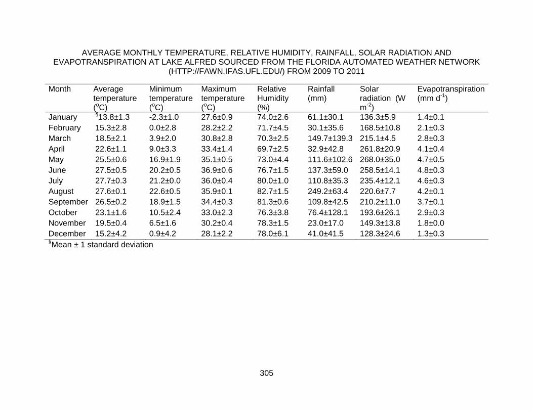
305
AVERAGE MONTHLY TEMPERATURE, RELATIVE HUMIDITY, RAINFALL, SOLAR RADIATION AND EVAPOTRANSPIRATION AT LAKE ALFRED SOURCED FROM THE FLORIDA AUTOMATED WEATHER NETWORK
(HTTP://FAWN.IFAS.UFL.EDU/) FROM 2009 TO 2011
Month Average temperature (oC)
Minimum temperature (oC)
Maximum temperature (oC)
Relative Humidity (%)
Rainfall (mm)
Solar radiation (W m-2)
Evapotranspiration (mm d-1)
January §13.8±1.3 -2.3±1.0 27.6±0.9 74.0±2.6 61.1±30.1 136.3±5.9 1.4±0.1
February 15.3±2.8 0.0±2.8 28.2±2.2 71.7±4.5 30.1±35.6 168.5±10.8 2.1±0.3
March 18.5±2.1 3.9±2.0 30.8±2.8 70.3±2.5 149.7±139.3 215.1±4.5 2.8±0.3
April 22.6±1.1 9.0±3.3 33.4±1.4 69.7±2.5 32.9±42.8 261.8±20.9 4.1±0.4
May 25.5±0.6 16.9±1.9 35.1±0.5 73.0±4.4 111.6±102.6 268.0±35.0 4.7±0.5
June 27.5±0.5 20.2±0.5 36.9±0.6 76.7±1.5 137.3±59.0 258.5±14.1 4.8±0.3
July 27.7±0.3 21.2±0.0 36.0±0.4 80.0±1.0 110.8±35.3 235.4±12.1 4.6±0.3
August 27.6±0.1 22.6±0.5 35.9±0.1 82.7±1.5 249.2±63.4 220.6±7.7 4.2±0.1
September 26.5±0.2 18.9±1.5 34.4±0.3 81.3±0.6 109.8±42.5 210.2±11.0 3.7±0.1
October 23.1±1.6 10.5±2.4 33.0±2.3 76.3±3.8 76.4±128.1 193.6±26.1 2.9±0.3
November 19.5±0.4 6.5±1.6 30.2±0.4 78.3±1.5 23.0±17.0 149.3±13.8 1.8±0.0
December 15.2±4.2 0.9±4.2 28.1±2.2 78.0±6.1 41.0±41.5 128.3±24.6 1.3±0.3 §Mean ± 1 standard deviation

306
APPENDIX F CORRELATIONS BETWEEN RLD MEASURED BY LINE INTERSECTION METHOD AND PREDICTED RLD BY SCANNING METHOD AND SCANNED AREA AT CREC
FOR ROOT DIAMETER LESS THAN 0.5 MM
Scanned area (pixels2)
0.0 5.0e+4 1.0e+5 1.5e+5 2.0e+5 2.5e+5 3.0e+5 3.5e+5
Ro
ot
leng
th d
ensi
ty (
cm c
m-3
)
0.0
0.2
0.4
0.6
0.8
1.0
1.2
1.4
1.6
Root density for roots with diameter <0.5 mm
Root length density by intercept method (cm cm-3
)
0.0 0.5 1.0 1.5 2.0 2.5
Pre
dic
ted
ro
ot
len
gth
den
sity
(cm
cm
-3)
0.0
0.5
1.0
1.5
2.0
2.5
3.0
RLD-intercept vs RLD-calibration set (root size <0.5mm)

307
CORRELATIONS BETWEEN RLD MEASURED BY LINE INTERSECTION METHOD AND PREDICTED RLD BY SCANNING METHOD AND SCANNED AREA AT CREC
FOR ROOT DIAMETER 0.5-1.0 MM
Scanned area (pixels2)
0 5000 10000 15000 20000 25000 30000 35000
Roo
t len
gth
dens
ity (c
m c
m-3
)
0.00
0.02
0.04
0.06
0.08
0.10
0.12
Root length density for medium size (0.5-1.0mm)
Root length density estimated by intecept method (cm cm-3
)
0.00 0.02 0.04 0.06 0.08 0.10 0.12 0.14 0.16
Pre
dic
ted
ro
ot
len
gth
den
sity
(cm
cm
-3)
0.00
0.02
0.04
0.06
0.08
0.10
0.12
0.14
RLD intercept-medium vs RLD predicted for root size (0.5-1.0 mm)
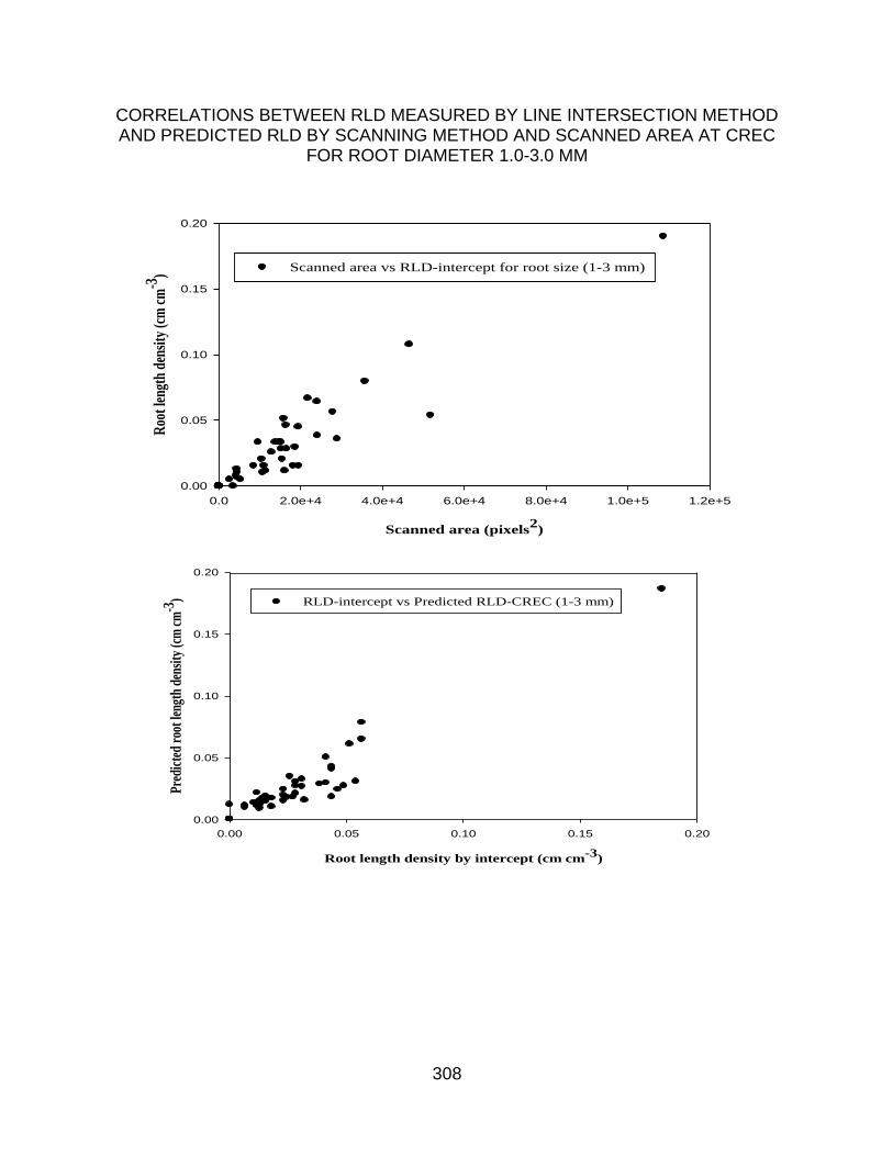
308
CORRELATIONS BETWEEN RLD MEASURED BY LINE INTERSECTION METHOD AND PREDICTED RLD BY SCANNING METHOD AND SCANNED AREA AT CREC
FOR ROOT DIAMETER 1.0-3.0 MM
Scanned area (pixels2
)
0.0 2.0e+4 4.0e+4 6.0e+4 8.0e+4 1.0e+5 1.2e+5
Roo
t le
ngth
den
sity
(cm
cm
-3)
0.00
0.05
0.10
0.15
0.20
Scanned area vs RLD-intercept for root size (1-3 mm)
Root length density by intercept (cm cm-3
)
0.00 0.05 0.10 0.15 0.20
Pre
dict
ed r
oot l
engt
h de
nsit
y (c
m c
m-3
)
0.00
0.05
0.10
0.15
0.20
RLD-intercept vs Predicted RLD-CREC (1-3 mm)

309
CORRELATIONS BETWEEN RLD MEASURED BY LINE INTERSECTION METHOD AND PREDICTED RLD BY SCANNING METHOD AND SCANNED AREA AT CREC
FOR ROOT DIAMETER GREATER THAN 3.0 MM
Scanned area
0.0 2.0e+4 4.0e+4 6.0e+4 8.0e+4 1.0e+5 1.2e+5
Roo
t len
gth
dens
ity (c
m c
m-3
)
0.000
0.002
0.004
0.006
0.008
0.010
0.012
0.014
0.016
0.018
0.020
Scanned area vs RLD intercept >3 mm
Root length density measured by intercept method (cm cm-3
)
0.000 0.005 0.010 0.015 0.020 0.025
Pre
dict
ed r
oot l
engt
h de
nsit
y (c
m c
m-3
)
0.000
0.002
0.004
0.006
0.008
0.010
0.012
RLD-intercept vs RLD-predicted at CREC >3mm

310
CORRELATIONS BETWEEN RLD MEASURED BY LINE INTERSECTION METHOD AND PREDICTED RLD BY SCANNING METHOD AND SCANNED AREA AT SWFREC
FOR ROOT DIAMETER LESS THAN 0.5 MM
Scanned area (pixels2
)
0 5e+4 1e+5 2e+5 2e+5 3e+5 3e+5
Roo
t len
gth
dens
ity (c
m c
m-3
)
0.0
0.1
0.2
0.3
0.4
0.5
0.6
0.7
Scanned data vs RLD intercept < 0.5 mm
Root length density by intercept (cm cm-3
)
0.0 0.1 0.2 0.3 0.4 0.5 0.6
Pre
dic
ted
roo
t le
ngt
h d
ensi
ty (
cm c
m-3
)
0.0
0.1
0.2
0.3
0.4
0.5
0.6
0.7
RLD-intercept vs RLD-predicted <0.5 mm

311
CORRELATIONS BETWEEN RLD MEASURED BY LINE INTERSECTION METHOD AND PREDICTED RLD BY SCANNING METHOD AND SCANNED AREA AT SWFREC
FOR ROOT DIAMETER 0.5-1.0 MM
Scanned area (pixels2)
0 2e+4 4e+4 6e+4 8e+4 1e+5
Roo
t len
gth
dens
ity
(cm
cm
-3)
0.00
0.02
0.04
0.06
0.08
0.10
0.12
0.14
0.16
0.18
Scanned area vs RLD intercept-0.5-1.0mm
Root length density-intercept (cm cm-3
)
0.00 0.05 0.10 0.15 0.20 0.25 0.30
Pre
dict
ed r
oot
leng
th d
ensi
ty (
cm c
m-3
)
0.00
0.05
0.10
0.15
0.20
0.25
RLD-intercept-medium vs Predicted RLD-medium
(0.5-1.0 mm)

312
CORRELATIONS BETWEEN RLD MEASURED BY LINE INTERSECTION METHOD AND PREDICTED RLD BY SCANNING METHOD AND SCANNED AREA AT SWFREC
FOR ROOT DIAMETER 1.0-3.0 MM
Scanned area (cm cm-3
)
0.0 2.0e+4 4.0e+4 6.0e+4 8.0e+4 1.0e+5 1.2e+5 1.4e+5
Roo
t len
gth
dens
ity
(cm
cm
-3)
0.00
0.02
0.04
0.06
0.08
0.10
0.12
0.14
Total area vs RLD-intercept-1-3mm
Root length density by intercept (cm cm-3
)
0.00 0.02 0.04 0.06 0.08 0.10 0.12 0.14 0.16 0.18
Pred
icte
d ro
ot le
ngth
den
sity
(cm
cm
-3)
0.00
0.02
0.04
0.06
0.08
0.10
0.12
0.14
RLD-intercept vs Predicted RLD (1.0-3.0 mm)

313
CORRELATIONS BETWEEN RLD MEASURED BY LINE INTERSECTION METHOD AND PREDICTED RLD BY SCANNING METHOD AND SCANNED AREA AT SWFREC
FOR ROOT DIAMETER GREATER THAN 3.0 MM
Scanned area (pixels2)
0 2e+4 4e+4 6e+4 8e+4 1e+5 1e+5 1e+5 2e+5 2e+5 2e+5
Roo
t len
gth
dens
ity (
cm c
m-3
)
0.00
0.01
0.02
0.03
0.04
0.05
Scanned area vs RLD-intercept->3 mm
Root length density by intercept (cm cm-3
)
0.000 0.005 0.010 0.015 0.020 0.025 0.030 0.035
Pre
dict
ed r
oot
leng
th d
ensi
ty (
cm c
m-3
)
0.000
0.005
0.010
0.015
0.020
0.025
0.030
RLD-intercept vs Predicted RLD->3 mm

314
APPENDIX G EXPERIMENTAL SET UP FOR THE SORPTION STUDY
Ion/Element Co1, µg/mL Co2, µg/mL Co3, µg/mL
P¶ 10 25 50 P§ 10 25 50 P§§ 5 25 50 K+ 6 32 63 NH4
+ 6 32 64 ¶Case A: In 20mL of 0.01M KCl §Case B: In 20mL of 0.005M CaCl2 §§Case C: In 20mL of fertilizer mixture

315
APPENDIX H SORPTION COEFFICIENTS FOR NH4
+ AND K+ ON IMMOKALEE AND CANDLER FINE SAND USING FERTILIZER MIXTURE IN TAP WATER
Soil Depth (cm) NH4+ K+
KD R2 KD R2
Immokalee 0-15 1.00 0.98 1.35 0.98
Immokalee 0-15 1.16 0.98 0.69 0.99
Immokalee 0-15 1.19 0.98 0.70 0.99
Immokalee 15-30 1.95 0.94 1.70 0.99
Immokalee 15-30 1.62 0.96 0.65 0.95
Immokalee 15-30 1.35 0.99 0.26 0.93
Candler 0-15 1.52 0.98 2.08 0.99
Candler 0-15 2.04 0.98 1.01 0.95
Candler 0-15 1.41 0.97 1.85 0.90
Candler 15-30 2.20 1.00 1.05 0.99
Candler 15-30 1.64 0.98 1.13 0.89
Candler 15-30 1.44 0.97 0.61 0.99

316
APPENDIX I SORPTION COEFFICIENTS FOR P ON IMMOKALEE AND CANDLER FINE SAND
Soil Electrolyte Depth (cm) Kf (mg1-N kg-1 LN) N †KD (L kg-1)
R2
Immokalee 0.01 M KCl 0-15 2.60 0.47 0.62 0.99 Immokalee 0.01 M KCl 0-15 1.36 0.56 0.41 0.99 Immokalee 0.01 M KCl 0-15 3.98 0.28 0.57 0.99 Immokalee 0.01 M KCl 15-30 1.56 0.55 0.46 0.98 Immokalee 0.01 M KCl 15-30 2.24 0.30 0.34 0.93 Immokalee 0.01 M KCl 15-30 2.79 0.49 0.70 0.99 Candler 0.01 M KCl 0-15 9.01 0.61 3.13 0.99 Candler 0.01 M KCl 0-15 7.41 0.58 2.38 0.96
Candler 0.01 M KCl 0-15 11.70 0.51 3.10 0.97
Candler 0.01 M KCl 15-30 19.33 0.48 4.73 0.98
Candler 0.01 M KCl 15-30 15.66 0.46 3.63 0.99
Candler 0.01 M KCl 15-30 13.04 0.46 3.02 0.97
Immokalee 0.005 M CaCl2 0-15 5.00 0.36 0.88 0.91 Immokalee 0.005 M CaCl2 0-15 3.25 0.45 0.73 0.98 Immokalee 0.005 M CaCl2 0-15 2.18 0.54 0.63 0.96 Immokalee 0.005 M CaCl2 15-30 3.56 0.42 0.74 0.99 Immokalee 0.005 M CaCl2 15-30 1.85 0.45 0.42 0.94 Immokalee 0.005 M CaCl2 15-30 3.97 0.51 1.05 0.95 Candler 0.005 M CaCl2 0-15 29.85 0.21 3.51 0.97 Candler 0.005 M CaCl2 0-15 18.04 0.31 2.78 0.97 Candler 0.005 M CaCl2 0-15 30.31 0.26 4.09 0.99 Candler 0.005 M CaCl2 15-30 31.02 0.23 3.86 0.99 Candler 0.005 M CaCl2 15-30 35.69 0.25 4.68 1.00 Candler 0.005 M CaCl2 15-30 33.39 0.28 4.75 0.96
Immokalee Fertilizer mixture 0-15 NA NA 0.56 1.00
Immokalee Fertilizer mixture 0-15 NA NA 0.41 0.95
Immokalee Fertilizer mixture 0-15 NA NA 0.38 0.99
Immokalee Fertilizer mixture 15-30 NA NA 0.26 0.91
Immokalee Fertilizer mixture 15-30 NA NA 0.37 0.86
Immokalee Fertilizer mixture 15-30 NA NA 0.65 0.98
Candler Fertilizer mixture 0-15 5.17 0.57 1.61 0.95
Candler Fertilizer mixture 0-15 7.84 0.43 1.67 0.94
Candler Fertilizer mixture 0-15 15.22 0.23 1.89 0.91
Candler Fertilizer mixture 15-30 2.73 0.69 1.18 0.98
Candler Fertilizer mixture 15-30 14.22 0.28 2.02 0.94
Candler Fertilizer mixture 15-30 14.6 0.41 2.95 0.99 †KD-Linearized KD estimated using a Cmax of 15 mg L-1 for Immokalee and Candler fine sand

317
LIST OF REFERENCES
Abrisqueta, J., O. Mounzer, S. Alvarez, W. Conejero, Y. Garcia-Orellana, L. Tapia, J. Vera, I. Abrisqueta, and M. Ruiz-Sanchez. 2008. Root dynamics of peach trees submitted to partial rootzone drying and continuous deficit irrigation. Agric. Water Manage. 95:959-967.
Afyuni, M., and M. Wagger. 2006. Soil physical properties and bromide movement in relation to tillage system. Commun. Soil. Sci. Plant Anal. 37:541-556.
Agyin-Birikorang, S., G. O'Connor, and S. Brinton. 2008. Evaluation phosphorus loss from a Florida Spodosol as affected by phosphorus-source application methods. J. Environ. Qual. 37:1180-1189.
Ahuja, L., D. Decoursey, B. Barnes, and K. Rojas. 1993. Characteristics of macropore transport studied with the ARS root-zone water-quality model. Trans. ASAE 36:369-380.
Allen, R.G., L.S. Pereira, D. Raes, and M. Smith. 1998. Crop evapotranspiration-Guidelines for computing crop water requirements. FAO, Rome.
Alva, A. 1993. Comparison of Mehlich-3, Mehlich-1, Ammonium bicarbonate-DTPA, 1.0M Ammonium acetate, and 0.2M Ammonium-chloride for extraction of calcium, magnesium, phosphorus, and potassium for a wide-range of soils. Commun. Soil. Sci. Plant Anal. 24:603-612.
Alva, A., and J. Syvertsen. 1991. Irrigation water salinity affects soil nutrient distribution, root density, and leaf nutrient levels of citrus under drip fertigation. J. Plant Nutr. 14:715-727.
Alva, A., S. Paramasivam, and W. Graham. 1998. Impact of nitrogen management practices on nutritional status and yield of Valencia orange trees and groundwater nitrate. J. Environ. Qual. 27:904-910.
Alva, A.K., and A. Fares. 1998. A new technique for continuous monitoring of soil moisture content to improve citrus irrigation. Proc. Fla. State Hort. Soc. 111:113-117.
Alva, A., O. Prakash, A. Fares, and A. Hornsby. 1999. Distribution of rainfall and soil moisture content in the soil profile under citrus tree canopy and at the dripline. Irrig. Sci. 18:109-115.
Alva, A., S. Paramasivam, W. Graham, and T. Wheaton. 2003. Best nitrogen and irrigation management practices for citrus production in sandy soils. Water Air Soil Pollut. 143:139-154.

318
Alva, A., K, S. Paramasivam, A. Fares, J.A. Delgado, D.J. Mattos, and K.S. Sajwan. 2005. Nitrogen and irrigation management practices to improve nitrogen uptake efficiency and minimize leaching losses. J. Crop Improvement 15:369-420.
Alva, A.K., and D.P.H. Tucker. 1997. Impact of soil pH and cations availability on citrus production in low buffered soils. Trends Soil Sci. 2:21-37.
Alva, A.K., and S. Paramasivam. 1998. An evaluation of nutrient removal by citrus fruits. Proc. Fla. State Hort. Sci. 111:126-128.
Alva, A.K., S. Paramasivam, T.A. Obreza, and A.W. Schumann. 2006a. Nitrogen best management practice for citrus trees - I. Fruit yield, quality, and leaf nutritional status. Sci. Hortic. 107:233-244.
Alva, A.K., S. Paramasivam, A. Fares, T.A. Obreza, and A.W. Schumann. 2006b. Nitrogen best management practice for citrus trees II. Nitrogen fate, transport, and components of N budget. Sci. Hortic. 109:223-233.
Alva, A.K., D.J. Mattos, S. Paramasivam, B. Patil, H. Dou, and K.S. Sajwan. 2006c. Potassium management for optimizing citrus production and quality. Int. J. Fruit Sci. 6:3-43.
Anderson, D., and L. Henderson. 1986. Sealed chamber digestion for plant nutrient analyses. Agron. J. 78:937-939.
Anderson, D., and L. Henderson. 1988. Comparing sealed chamber digestion with other digestion methods used for plant-tissue analysis. Agron. J. 80:549-552.
Andreu, L., J. Hopmans, and L. Schwankl. 1997. Spatial and temporal distribution of soil water balance for a drip-irrigated almond tree. Agricult. Water Manag. 35:123-146.
Angelakis, A., D. Rolston, T. Kadir, and V. Scott. 1993. Soil-water distribution under trickle source. J. Irrig. Drain. Div. Am. Soc. Civ. Eng. 119:484-500.
Arias Reveron, J., and H. Browning. 1995. Development and mortality of the citrus snow scale (homoptera, diaspididae) under constant-temperature and relative-humidity. Environ. Entomol. 24:1189-1195.
Aubert, B., M. Grisoni, M. Villemin, and G. Rossolin. 1996. A case study of Huanglongbing (greening) control in Reunion. p. 276-278 In J. V. da Graca, et al. (eds.) Proc. 13th Conference of the International Organization of Citrus Virologists (IOCV), University of California, Riverside1996.
Bacon, P., and B. Davey. 1989. Nutrient availability under trickle irrigation phosphate fertilization. Fert. Res. 19:159-167.

319
Badr, A.E., and M.E. Abuarab. 2011. Soil moisture distribution patterns under surface and subsurface drip irrigation systems in sandy soil using neutron scattering technique. Irrigation Science DOI 10.1007/s00271-011-0306-0.
Badr, M.A. 2007. Spatial distribution of water and nutrients in the root zone under surface and subsurface drip irrigation and cantaloupe yield. World J. Agric. Sci. 3:747-756.
Baker, J., and C. Vanbavel. 1987. Measurement of mass-flow of water in the stems of herbaceous plants. Plant Cell Environ. 10:777-782.
Baker, J., and J. Nieber. 1989. An analysis of the steady-state heat-balance method for measuring sap flow in plants. Agric. For. Meteorol. 48:93-109.
Barnette, R.M., E.F. DeBusk, J.B. Hester, and W.W. Jones. 1931. The mineral analysis of nineteen year old Marsh seedless grapefruit tree. Citrus Ind. 12:5-6.
Barraclough, P., and R. Leigh. 1984. The growth and activity of winter-wheat roots in the field - the effect of sowing date and soil type on root-growth of high-yielding crops. J. Agric. Sci. 103:59-74.
Barrow, N., J. Bowden, A. Posner, and J. Quirk. 1980. Describing the effects of electrolyte on adsorption of phosphate by a variable charge surface. Aust. J. Soil Res. 18:395-404.
Baryosef, B., and M. Sheikholslami. 1976. Distribution of water and ions in soils irrigated and fertilized from a trickle source Soil Sci. Soc. Am. J. 40:575-582.
Baryosef, B., and B. Akiri. 1978. Sodium-bicarbonate extraction to estimate nitrogen, phosphorus, and potassium availability in soils. Soil Sci. Soc. Am. J. 42:319-323.
Baryosef, B., S. Schwartz, T. Markovich, B. Lucas, and R. Assaf. 1988. Effect of root volume and nitrate solution concentration on growth, fruit yield, and temporal N and water-uptake rates by apple-trees. Plant Soil 107:49-56.
Bassoi, L.H., J.W. Hopmans, L.A.C. Jorge, C.M. Alencar, and J.A.M. Silva. 2003. Grapevine root distribution in drip and microsprinkler irrigation. Sci. Agric. 60:377-387.
Bauer, L.R., and K.J. Hamby. 2003. Relative sensitivities of existing and novel model parameters in atmospheric tritium dose estimates. Radiat. Prot. Dosimetry 37:253-260.
Bauer, M.G., W.S. Castle, B.J. Boman, T.A. Obreza, and E.W. Stover. 2004. Root systems of healthy and declining citrus trees on swingle citrumelo rootstock growing in the southern Florida flatwoods. Proc. Fla. State Hort. Soc. 117:103-109.

320
Belmont, M., J. White, and K. Reddy. 2009. Phosphorus Sorption and Potential Phosphorus Storage in Sediments of Lake Istokpoga and the Upper Chain of Lakes, Florida, USA. J. Environ. Qual. 38:987-996.
Bland, W., and M. Mesarch. 1990. Counting error in the line-intercept method of measuring root length. Plant Soil 125:155-157.
Bloom, S.A. 2009. Water release curve fitting using CAS. Gainesville, Florida, USA
Boesch, D., R. Brinsfield, and R. Magnien. 2001. Chesapeake Bay eutrophication: Scientific understanding, ecosystem restoration, and challenges for agriculture. J. Environ. Qual. 30:303-320.
Bogren, K. and P. Smith. 2003. Determination of bromide by flow injection analysis. QuickChem Method 10-135-214-2-B. Lachat Instruments 5600 Lindburgh Drive, Loveland, Colorado, USA.
Boivin, A., J. Simunek, M. Schiavon, and M. van Genuchten. 2006. Comparison of pesticide transport processes in three tile-drained field soils using HYDRUS-2D. Vadose Zone J. 5:838-849.
Boland, A., P. Jerie, P. Mitchell, and I. Goodwin. 2000. Long-term effects of restricted root volume and regulated deficit irrigation on peach: I. Growth and mineral nutrition. J. Am. Soc. Hortic. Sci.125:135-142.
Boman, B.J. 1994. Evapotranspiration by young Florida flatwoods citrus trees. J. Irrig. Drain. Div. Am. Soc. Civ. Eng. 120:80-88.
Bove, J. 2006. Huanglongbing: A destructive, newly-emerging, century-old disease of citrus. J. Plant Pathol. 88:7-37.
Bowman, B.T. 1982. Conversion of Freundlich adsorption K values to the mole fraction format and the use of SY values to express relative adsorption of pesticides. Soil Sci. Soc. Am. J. 46:740-743.
Bowman, R., M. Essington, and G. Oconnor. 1981. Soil sorption of nickel - influence of solution composition. Soil Sci. Soc. Am. J. 45:860-865.
Brooks, R.H., and A.T. Corey. 1964. Hydraulic properties of porous media Hydrology paper No 3, Colorado State University, Fort Collins.
Bryla, D., T. Trout, J. Ayars, and R. Johnson. 2003. Growth and production of young peach trees irrigated by furrow, microjet, surface drip, or subsurface drip systems. HortScience 38:1112-1116.
Bryla, D., E. Dickson, R. Shenk, R. Johnson, C. Crisosto, and T. Trout. 2005. Influence of irrigation method and scheduling on patterns of soil and tree water status and its relation to yield and fruit quality in peach. HortScience 40:2118-2124.

321
Bufon, V.B., R.J. Lascano, C. Bednarz, J.D. Booker, and D.C. Gitz. 2011. Soil water content on drip irrigated cotton: comparison of measured and simulated values obtained with the Hydrus 2-D model. Irrig. Sci. DOI: 10.1007/s00271-011-0279.
Calvert, D.V., H.W. Ford, E.H. Stewart, and F.G. Martin. 1977. Growth response of twelve citrus rootstock-scion combinations on a Spodosol modified by deep tillage and profile drainage. Int. Soc. Citric. 1:79-84.
Cameron, S., and O. Compton. 1945. Nitrogen in bearing orange trees. Proc. Am. Soc. Hortic. Sci. 46:60-68.
Cameron, S.H., and D. Appleman. 1935. The distribution of total nitrogen in the orange tree. Proc. Am. Soc. Hortic. Sci. 30:341-348.
Camp, C. 1998. Subsurface drip irrigation: A review. Trans. ASAE 41:1353-1367.
Campbell, G. 1974. Simple method for determining unsaturated conductivity from moisture retention data. Soil Sci. 117:311-314.
Carlisle, V.W., F. Sodek, M. Collins, L.C. Hammond, and W.G. Harris. 1989a. Characterization data for selected Florida Soils. Gainesville, University of Florida, Florida.
Carlisle, V.W., F. Sodek, M. Collin, L.C. Hammond, and W.G. Harris. 1989b. Characterization data for selected Florida soils. University of Florida, Gainesville, FL.
Carrasco, G., O. Marquez, M. Urrestarazu, and M.C. Salas. 2003. Transplants grown hydroponically are an alternative for soil. Acta Hortic. :407-410.
Carsel, R., and R. Parrish. 1988. Developing joint probability-distributions of soil-water retention characteristics. Water Resour. Res. 24:755-769.
Cassel, D.K., and D.R. Nielsen. 1986. Field capacity and available water capacity, p. 901-926, In A. Klute, (ed.) Methods of Soil Analysis Part 1 2nd edition. ed. Agronomy Ser. 9. Madison, Wisconsin, USA.
Castel, J.R., I. Bautista, C. Ramos, and G. Cruz. 1987. Evapotranspiration and irrigation efficiency of mature orange orchards in Valencia (Spain). Irrig. Drain. Syst. 3:205-217.
Castle, W.S. 1980. Citrus rootstocks for tree size control and higher density plantings in Florida. Proc. Fla. State Hort. Soc. 93:24-27.
Castle, W.S. and A.H. Krezdorn. 1975. Effect of citrus rootstocks on root distribution and leaf mineral content of ‘Orlando’ tangelo tree. J. Amer. Soc. Hort. Sci. 100:1-4.

322
Charanjeet, S., and D.K. Das. 1985. Nitrate-nitrogen distribution in soil and nitrogen uptake by wheat under varying levels of water and nitrogen supply. Ann. Agric. Res. 6:91-97.
Chung, K.R., and R.H. Brlansky. 2009. Citrus diseases exotic to Florida: Huanglongbing (Citrus Greening), PP210 ed. UF/IFAS Extension Cooperative Service, Gainesville, Florida.
Clark, C., and A. Richardson. 2002. Biomass and mineral nutrient partitioning in a developing tamarillo (Cyphomandra betacea) crop. Sci. Hortic. 94:41-51.
Clemente, R., R. Dejong, H. Hayhoe, W. Reynolds, and M. Hares. 1994. Testing and comparison of 3 unsaturated soil-water flow models. Agric. Water Manage. 25:135-152.
Clothier, B., and T. Sauer. 1988. Nitrogen transport during drip fertigation with urea. Soil Sci. Soc. Am. J. 52:345-349.
Clothier, B., T. Sauer, and S. Green. 1988. The movement of ammonium-nitrate into unsaturated soil during unsteady absorption. Soil Sci. Soc. Am. J. 52:340-345.
Coleman, M. 2007. Spatial and temporal patterns of root distribution in developing stands of four woody crop species grown with drip irrigation and fertilization. Plant Soil 299:195-213.
Collins, R., P. Gregory, H. Rowse, A. Morgan, and B. Lancashire. 1987. Improved methods of estimating root length using a photocopier, a light box and a bar code reader. Plant Soil 103:277-280.
Consoli, S., N. O'Connell, and R. Snyder. 2006. Estimation of evapotranspiration of different-sized navel-orange tree orchards using energy balance. J. Irrig. Drain. Div. Am. Soc. Civ. Eng. 132:2-8.
da Graca, J., and L. Korsten. 2004. Citrus huanglongbing: Review, present status and future strategies. Diseases Fruit Vegetables 1:229-245.
Dasberg, S. 1987. Nitrogen-fertilization in citrus orchards. Plant Soil 100:1-9.
Davenport, J., R. Stevens, and K. Whitley. 2008. Spatial and temporal distribution of soil moisture in drip-irrigated vineyards. HortScience 43:229-235.
De Jong, R., G.C. Topp, and W.D. Reynolds. (eds.) 1992. The use of measured and estimated hydraulic properties in the simulation of soil and water movement - a case study. US Department of Agriculture and Department of Soil and Environmental Sciences, University of California, Riverside.

323
De Silva, H., A. Hall, D. Tustin, and P. Gandar. 1999. Analysis of distribution of root length density of apple trees on different dwarfing rootstocks. Ann. Bot. 83:335-345.
Decoursey, D.G., and K.W. Rojas. 1990. RZWQM-A model for simulating the movement of water and in solutes in the root zone. p. 813-821 In D. G. Decoursey (ed.) Proc. International Symposium on Water Quality Modeling of Agricultural Nonpoint Sources, Washington, DC.1990. USDA-Agricultural Research Service ARS-81, Washington, DC.
Devitt, D., M. Berkowitz, P. Schulte, and R. Morris. 1993. Estimating transpiration for 3 woody ornamental tree species using stem-flow gauges and lysimetry. HortScience 28:320-322.
Elrashidi, M., A. Alva, Y. Huang, D. Calvert, T. Obreza, and Z. He. 2001. Accumulation and downward transport of phosphorus in Florida soils and relationship to water quality. Commun. Soil. Sci. Plant Anal. 32:3099-3119.
Embleton, T.W., J.D. Kirkpatrick, W.W. Jones, and C.B. Cree. 1956. Influence of applications of dolomite, potash and phosphate on yield and size of fruit and on composition of leaves of Valencia orange trees. Proc. Amer. Soc. Hort. Sci. 67:183-190.
Essington, M.E. 2004. Soil and water chemistry: an integrative approach CRC Press, Boca Raton, FL.
Falivene, S. 2005. Open hydroponics: risks and opportunities. Land and Water Australia through the National Program of Sustainable Irrigation, Australia. http://www.arapahocitrus.com/files/OHS_Stage_Publications.pdf
Falivene, S., I. Goodwin, D. Williams, and A.M. Boland. 2005. Open hydroponics: risks and opportunities. Stage 1: General principles and literature review. http://www.arapahocitrus.com/files/OHS_Stage_Publications.pdf
Fandika I.R., D. Kadyampakeni, and S. Zingore. 2012. Performance of bucket drip irrigation by treadle pump on tomato and maize/bean production in Malawi. Irrig. Sci. 30:57–68.
Fares, A., and A. Alva. 1999. Estimation of citrus evapotranspiration by soil water mass balance. Soil Sci. 164:302-310.
Fares, A., and A. Alva. 2000a. Evaluation of capacitance probes for optimal irrigation of citrus through soil moisture monitoring in an Entisol profile. Irrig. Sci. 19:57-64.
Fares, A., and A. Alva. 2000b. Soil water components based on capacitance probes in a sandy soil. Soil Sci. Soc. Am. J. 64:311-318.

324
Fares, A., J. Simunek, M.T. van Genuchten, L.R. Parsons, T.A. Wheaton, and K.T. Morgan. 2001. Effect of emitter patterns on solute transport. Soil Crop Sci. Soc. Proc. 61:46-56.
Fares, A., A. Dogan, F. Abbas, L. Parsons, T. Obreza, and K. Morgan. 2008. Water balance components in a mature citrus orchard. Soil Sci. Soc. Am. J. 72:578-585.
Fassel, V., and R. Kniseley. 1974. Inductively coupled plasma - optical emission-spectroscopy. Anal. Chem. 46:1110-1120.
Feddes, R.A., P.J. Kowalik, and H. Zaradny. 1978. Simulation of field water use and crop yield John Wiley and Sons, New York, USA.
Feigenbaum, S., H. Bielorai, Y. Erner, and S. Dasberg. 1987. The fate of N-15 labeled nitrogen applied to mature citrus trees. Plant Soil 97:179-187.
Ferguson, J.J. 2002. Young Florida dooryard citrus guide-young tree care. Gainesville, FL.
Ferguson, J.J., F.S. Davies, C.H. Matthews, and R.M. Davis. 1988. Controlled-release fertilizers and growth of young 'Hamlin' orange trees. Proc. Fla. State Hort. Soc. 101:17-20.
Fernandez-Galvez, J., and L. Simmonds. 2006. Monitoring and modelling the three-dimensional flow of water under drip irrigation. Agric. Water Manage. 83:197-208.
Ford, H.W. 1954. Root distribution in relation to the water table. Proc. Fla. State Hort. Soc. 67:30-33.
Ford, H.W. 1964. The effect of root stock, soil and soil pH on citrus root growth in soils subject to flooding. Proc. Fla. State Hort. Soc. 77:41-45.
Ford, H.W. 1972. Eight years of root injury from water table fluctuations. Proc. Fla. State Hort. Soc. 85:65-68.
Gardenas, A., J. Hopmans, B. Hanson, and J. Simunek. 2005. Two-dimensional modeling of nitrate leaching for various fertigation scenarios under micro-irrigation. Agric. Water Manage. 74:219-242.
Garnier, P. 2003. Sensitivity analysis of PASTIS, a model of nitrogen transport in the soil, p. 367-375, In D. Wallach, et al., (eds.) Working with Dynamic Models: application, analysis, parameterization, and applications. ed., Amsterdam, The Netherlands.
Goldberg, D., and M. Shmueli. 1970. Drip irrigation-a method used under arid and desert conditions of high water and soil salinity. Trans. ASAE 13:38-41.

325
Goldberg, S., M. Rinot, and N. Karu. 1971. Effect of trickle irrigation intervals on distribution and utilization of soil moisture in a vineyard. Soil Sci. Soc. Am. Proc. 35:127-&.
Gottwald, T., J. Graham, and T. Schubert. 2002a. Citrus canker: The pathogen and its impact. American Phytopathological Society, St. Paul, Minnesota.
Gottwald, T., X. Sun, T. Riley, J. Graham, F. Ferrandino, and E. Taylor. 2002b. Geo-referenced spatiotemporal analysis of the urban citrus canker epidemic in Florida. Phytopathology 92:361-377.
Graetz, D.A., and V.D. Nair. 2009. Phosphorus sorption isotherm determination, p. 33-37, In J. L. Kovar and G. M. Pierzynski, (eds.) Methods of P Analysis for Soils, Sediments, Residuals, and Waters 2nd ed. Virginia Tech University, Blacksburg, Virginia.
Graser, E.A., and L.H. Allen. 1987. Water management for citrus production in the Florida Flatwoods. Proc. Fla. State Hort. Soc. 100:126-136.
Grieve, A. 1989. Water-use efficiency, nutrient-uptake and productivity of micro-irrigated citrus. Austr. J. Exp. Agric. 29:111-118.
Grosse, W., F. Wissing, R. Perfler, Z. Wu, J. Chang, and Z. Lei. 1999. Biotechnological approach to water quality improvement in tropical and subtropical areas for reuse and rehabilitation of aquatic ecosystems. Cologne, Germany.
Gutierrez, M., and F. Meinzer. 1994. Estimating water-use and irrigation requirements of coffee in Hawaii. Journal of the American Society For Horticultural Science 119:652-657.
Gutierrez, M., R. Harrington, F. Meinzer, and J. Fownes. 1994. The effect of environmentally-induced stem temperature-gradients on transpiration estimates from the heat-balance method in 2 tropical woody species. Tree Physiol. 14:179-190.
Halbert, S., and K. Manjunath. 2004. Asian citrus psyllids (Sternorrhyncha : Psyllidae) and greening disease of citrus: A literature review and assessment of risk in Florida. Fla. Entomol. 87:330-353.
Ham, J., J. Heilman, and R. Lascano. 1990. Determination of soil-water evaporation and transpiration from energy-balance and stem-flow measurements. Agric. For. Meteorol. 52:287-301.
Hanlon, E.A., J.S. Gonzalez, and J.M. Bartos. 1997. Mehlich 1 extractable P, Ca, Mg, Mn, Cu and Zn. University of Florida, Gainesville, FL.

326
Hanson, B., J. Simunek, and J. Hopmans. 2006. Evaluation of urea-ammonium-nitrate fertigation with drip irrigation using numerical modeling. Agric. Water Manage. 86:102-113.
Harbridge, J. 2007a. Determination of nitrate in 2M KCl soil extracts by flow injection analysis QuickChem Method 12-107-04-1-J. Lachat Instruments 5600 Lindburgh Drive, Loveland, Colorado, USA.
Harbridge, J. 2007b. Determination of ammonia in 2M KCl soil extracts by flow injection analysis QuickChem Method 12-107-04-1-J. Lachat Instruments 5600 Lindburgh Drive, Loveland, Colorado, USA.
Harris, W., R. Rhue, G. Kidder, R. Brown, and R. Littell. 1996. Phosphorus retention as related to morphology of sandy coastal plain soil materials. Soil Sci. Soc. Am. J. 60:1513-1521.
Havlin, J.L., J.D. Beaton, S.L. Tisdale, and W.L. Nelson. 2005. Soil fertility and fertilizers: An introduction to nutrient management. 7th ed., Prentice Hall, New Delhi.
He, Z., D. Calvert, A. Alva, D. Banks, and Y. Li. 2000. Nutrient leaching potential of mature grapefruit trees in a sandy soil. Soil Sci. 165:748-758.
Heilman, J., K. Mcinnes, M. Savage, R. Gesch, and R. Lascano. 1994. Soil and canopy energy balances in a west texas vineyard. Agric. For. Meteorol. 71:99-114.
Hillel, D. 1998. Environmental Soil Physics Academic Press, San Diego, CA.
Himmelbauer, M., W. Loiskandl, and F. Kastanek. 2004. Estimating length, average diameter and surface area of roots using two different Image analyses systems. Plant Soil 260:111-120.
Hoffman, G.J., J.D. Oster, and W.J. Alves. 1982. Evapotranspiration of Mature Orange Trees Under Drip Irrigation in an Arid Climate. Trans. ASAE 25:992-996.
Hornsby, A.G., P.S.C. Rao, J.G. Booth, P.V. Rao, K.D. Pennell, R.E. Jessup, and G.D. Means. 1990. Evaluation of models for predicting fate of pesticides. Soil Science Department and Statistics Department, University of Florida, Tallahasee, FL.
Huntington, T.G., A.H. Johnson, and T.N. Schwartzman. 1990. Mechanical vacuum extraction vs. batch equilibration for estimation of exchangeable cations. Soil Sci. Soc. Am. J. 54:381-385.
Hutson, J., and R. Wagenet. 1991. Simulating nitrogen dynamics in soils using a deterministic model. Soil Use Manage. 7:74-78.

327
Hutson, J.L. 2005. Leaching and Chemistry Model (LEACHM): A process-based model of water and solute movement, transformations, plant uptake and chemical reactions in the unsaturated zone. Cornell University, Ithaca, New York.
Irey, M., P. Mai, J. Graham, and J. Johnson. 2008. Data trends and results from an HLB testing laboratory that has processed over 64,000 commercial and research samples over a two year period in Florida. Abstract IRCHLB Proc. 103.
Ismail, M., and K. Noor. 1996. Growth, water relations and physiological processes of starfruit (Averrhoa carambola L) plants under root growth restriction. Sci. Hortic. 66:51-58.
Jabro, J., J. Jemison, L. Lengnick, R. Fox, and D. Fritton. 1993. Field validation and comparison of leachm and ncswap models for predicting nitrate leaching. Trans. ASAE 36:1651-1657.
Jansson, P.E., and L. Karlberg. 2001. Coupled heat and mass transfer model for soil-plant-atmosphere systems. Royal Institute, Stockholm.
Jia, X., A. Swancar, J.A. Jacobs, M.D. Dukes, and K. Morgan. 2007. Comparison of evapotranspiration rates for flatwoods and ridge citrus. Trans. ASABE 50:83-94.
Jones, J., G. Hoogenboom, C. Porter, K. Boote, W. Batchelor, L. Hunt, P. Wilkens, U. Singh, A. Gijsman, and J. Ritchie. 2003. The DSSAT cropping system model. Eur. J. Agron. 18:235-265.
Jones, J.B. 1997. Hydroponics: A practical guide for the soilless grower St. Lucie Press, FL.
Jones, J.B.J., and V.W. Case. 1990. Sample, handling, and analyzing plant tissue samples, p. 389-427, In R. L. Westerman, (ed.) Soil Testing and Plant Analysis. ed. Soil Science Society of America, Madison, Wisconsin.
Kadlec, R.H., and R.L. Knight. 1996. Treatment wetlands CRC Press, Boca Raton, FL, USA.
Kalmar, D., and E. Lahav. 1977. Water requirements of avocado in Israel .1. Tree and soil parameters. Austr. J. Agric. Res. 28:859-868.
Kandelous, M., and J. Simunek. 2010a. Comparison of numerical, analytical, and empirical models to estimate wetting patterns for surface and subsurface drip irrigation. Irrig. Sci. 28:435-444.
Kandelous, M., and J. Simunek. 2010b. Numerical simulations of water movement in a subsurface drip irrigation system under field and laboratory conditions using HYDRUS-2D. Agric. Water Manage. 97:1070-1076.

328
Kandelous, M., J. Simunek, M. van Genuchten, and K. Malek. 2011. Soil water content distributions between two emitters of a subsurface drip irrigation system. Soil Sci. Soc. Am. J. 75:488-497.
Katul, G., P. Todd, D. Pataki, Z. Kabala, and R. Oren. 1997. Soil water depletion by oak trees and the influence of root water uptake on the moisture content spatial statistics. Water Resour. Res. 33:611-623.
Keller, J., and D. Karmeli. 1974. Trickle irrigation design for optimal soil wetting. Proc. International Drip Irrigation Congress, San Diego, California, USA.
Khakural, B., and A. Alva. 1996. Transformation of urea and ammonium nitrate in an Entisol and a Spodosol under citrus production. Commun. Soil. Sci. Plant Anal. 27:3045-3057.
Khan, A., M. Yitayew, and A. Warrick. 1996. Field evaluation of water and solute distribution from a point source. J. Irrig. Drain. Div. Am. Soc. Civ. Eng. 122:221-227.
Kiggundu, N., K.W. Migliaccio, B. Schaffer, Y. Li, and J.H. Crane. 2011. Water savings, nutrient leaching, and fruit yield in ayoung avocado orchard as affected by irrigation and nutrient management. Irrig. Sci. DOI: 10.1007/s00271-011-0280-6.
Kirchoff, G. 1992. Measurement of root length and thickness using a handheld counter scanner. Field Crops Res. 29:79-88.
Klein, I., and G. Spieler. 1987. Fertigation of apples with nitrate or ammonium nitrogen under drip irrigation .2. Nutrient distribution in the soil. Commun. Soil. Sci. Plant Anal. 18:323-339.
Klein, I., A. Meimon, and D. Skedi. 1999. Drip nitrogen, phosphorus, and potassium fertigation of 'Spadona' pear. J. Plant Nutr. 22:489-499.
Klepper, B. 1992. Development and growth of crop root systems. Adv. Soil Sci. 19:1-25.
Klute, A. 1986. Water retention: Laboratory methods, p. 635-662, In A. Klute, (ed) Methods of soil analysis. Part 1. Physical and Mineralogical Methods. Agronomy No. 9. 2nd ed. American Society of Agronomy, Madison, WI.
Klute, A. and C. Dirksen. 1986. Hydraulic conductivity and diffusivity: laboratory methods, p. 687-734, In A. Klute (ed.) Methods of soil analysis. Part 1. Physical and Mineralogical Methods. Agronomy No. 9. 2nd ed. American Society of Agronomy, Madison, WI.
Kohne, J., and H. Gerke. 2005. Spatial and temporal dynamics of preferential bromide movement towards a tile drain. Vadose Zone J. 4:79-88.

329
Koo, R.C.J. 1980. Results of citrus fertigation studies. Proc. Fla. State Hort. Sci. 93:33-36.
Koo, R.C.J., and A.G. Smajstrla. 1984. Effects of trickle irrigation and fertigation on fruit production and juice quality of 'Valencia' orange. Proc. Fla. State Hort. Soc. 97:8-10.
Koo, R.C.J., C.A. Anderson, I. Stewart, D.P.H. Tucker, D.V. Calvert, and H.K. Wutscher. 1984. Recommended fertilizer and nutrional sprays for citrus. Gainesville, Florida.
Kruger, J.A., C.D. Tolmay. and K. Britz. 2000a. Effects of fertigation frequencies and irrigation systems on performance of' Valencia' oranges in two subtropical areas of South Africa. Proc. Int. Soc. Citric. Congr. p. 232-235.
Kruger, J.A., K. Britz, C.D. Tolmay, and S F. du Plessis. 2000b. Evaluation of an open hydroponics system (OHS) for citrus in South Africa: Preliminary results. Proc. Int. Soc. Citric. Congr. p. 239-242.
Kuperus, K.H., N. Combrink, K. Britz, and J. Ngalo. 2002. Evaluation of an open hydroponics system (OHS) for citrus in South Africa: Preliminary results, pp. 239-242 Annual Research Report. Citrus Research International (Pty) Ltd.
Kusakabe, A., S. White, J. Walworth, G. Wright, and T. Thompson. 2006. Response of microsprinkler-irrigated navel oranges to fertigated nitrogen rate and frequency. Soil Sci. Soc. Am. J. 70:1623-1628.
Lamb, S., W. Graham, C. Harrison, and A. Alva. 1999. Impact of alternative citrus management practices on groundwater nitrate in the Central Florida Ridge - I. Field investigation. Trans. ASAE 42:1653-1668.
Lascano, R., R. Baumhardt, and W. Lipe. 1992. Measurement of water-flow in young grapevines using the stem heat-balance method. Am. J. Enol. Vitic. 43:159-165.
Lea-Cox, J.D., J.P. Syvertsen, and D.A. Graetz. 2001. Springtime 15Nitrogen uptake, partitioning, and leaching losses from young bearing Citrus trees of differing nitrogen status. J. Amer. Soc. Hort. Sci. 126:242-251.
Legaz, F., M. Serna, and E. Primomillo. 1995. Mobilization of the reserve in citrus. Plant Soil 173:205-210.
Legaz, F., E. Primomillo, E. Primoyufera, C. Gil, and J. Rubio. 1982. Nitrogen-fertilization in citrus .1. Absorption and distribution of nitrogen in calamondin trees (Citrus-mitis BL), during flowering, fruit-set and initial fruit-development periods. Plant Soil 66:339-351.

330
Li, J., and Y. Liu. 2011. Water and nitrate distributions as affected by layered-textural soil and buried dripline depth under subsurface drip fertigation. Irrig. Sci. 29:469-478.
Li, J., J. Zhang, and L. Ren. 2003. Water and nitrogen distribution as affected by fertigation of ammonium nitrate from a point source. Irrig. Sci. 22:19-30.
Ling, G., and A. El-Kadi. 1998. A lumped parameter model for nitrogen transformation in the unsaturated zone. Water Resour. Res. 34:203-212.
Lotse, E.,J. Jabro, K. Simmons, and D. Baker. 1992. Simulation of nitrogen dynamics and leaching from arable soils. J. Contam. Hydrol. 10:183-196.
Lu, J., and L. Wu. 2003. Visualizing bromide and iodide water tracer in soil profiles by spray methods. J.Environ. Qual. 32:363-367.
Lumbanraja, J., and V. Evangelou. 1990. Binary and ternary exchange behavior of potassium and ammonium on Kentucky subsoils. Soil Sci. Soc. Am. J. 54:698-705.
Lumbanraja, J., and V. Evangelou. 1994. Adsorption-desorption of potassium and ammonium at low cation concentrations in 3 Kentucky subsoils. Soil Sci. 157:269-278.
Manjunath, K.L., S.E. Halbert, C. Ramadugu, S. Webb, and R.F. Lee. 2008. Detection of ‘Candidatus Liberibacter asiaticus’ in Diaphorina citri and its importance in the management of citrus huanglongbing in Florida. Phytopathology 98:387-396.
Marler, T.E. and F.S. Davies. 1990. Microsprinkler Irrigation ‘Hamlin’ Orange Trees. J. Amer. Soc. Hort. Sci. 115(1):45-51.
Martin, E.C., A.K. Hla, P.M. Waller, and D.C. Slack. 1997. Heat unit-based crop coefficient for grape fruit trees. Appl. Eng. Agric. 13:485-489.
Martinez-Valero, R., and C. Fernandez. 2004. Preliminary results in citrus groves grown under the MOHT system. Int. Citrus Cong.103.
Masse J., F. Tardieu, and C. Colnenne. 1991. Rooting depth and spatial arrangement of roots in winter wheat. In McMichael B.L. and Persson H. (eds.) Plant Roots and their Environment, pp. 480-486. Amsterdam: Elsevier.
Mattos, D., D. Graetz, and A. Alva. 2003a. Biomass distribution and nitrogen-15 partitioning in citrus trees on a sandy entisol. Soil Sci. Soc. Am. J. 67:555-563.
Mattos, D., J.A. Quaggio, H. Cantarella, and A.K. Alva. 2003b. Nutrient content of biomass components of Hamlin sweet orange tree. Sci. Agric. 60:155-160.

331
Mattos, D., A. Alva, S. Paramasivam, and D. Graetz. 2003c. Nitrogen volatilization and mineralization in a sandy entisol of Florida under citrus. Commun. Soil. Sci. Plant Anal. 34:1803-1824.
Mattos Junior, D. 2000. Citrus response functions to N, P, and K fertilization and N uptake dynamics. Thesis (Ph D ), University of Florida, 2000.
Mattos, D., T.F. Milanze, F.A. Azevedo, J.A. Quaggio. 2010. Soil nutrient availability and its impact on fruit quality of Tahiti acid lime. Rev. Bras. Frutic. 32:335-342.
Mehlich, A. 1953. Determination of P, K, Ca, Mg, and NH4. Soil Test Div. Mimeo, N.C. Dept. of Agriculture, Raleigh. www.ncagr.com/agronomi/pdffiles/mehlich53.pdf
Meinzer, F., G. Goldstein, N. Holbrook, P. Jackson, and J. Cavelier. 1993. Stomatal and environmental-control of transpiration in a lowland tropical forest tree. Plant Cell Environ. 16:429-436.
Michelakis, N., E. Vougioucalou, and G. Clapaki. 1993. Water-use, wetted soil volume, root distribution and yield of avocado under drip irrigation. Agric. Water Manage. 24:119-131.
Migliaccio. K.C. and Y.C. Li. 2009. Irrigation scheduling for tropical fruit groves in south Florida. Univ. of Florida Coop. Ext. Serv., Fact Sheet TR001. Gainesville, FL.
Misra, C., D. Nielsen, and J. Biggar. 1974. Nitrogen transformations in soil during leaching .1. Theoretical considerations. Soil Sci. Soc. Am. J. 38:289-293.
Monod, H., C. Naud, and D. Makowski. 2003. Uncertainty and sensitivity analysis for crop models, p. 55-99, In D. Wallach, et al., (eds.) Working with Dynamic Crop Models: Application, Analysis, Parameterization, and Applications. ed., Amsterdam, The Netherlands.
Morgan, K. H. Beck, J. Scholberg, and S. Grunwald. 2006c. In-Season Irrigation and Nutrient Decision Support System for Citrus Production. In F. Zazueta, J. Kin, S. Ninomiya and G. Schiefer (eds) Computers in Agriculture and Natural Resources, Proceedings of the 4th World Congress, 24-26 July 2006, Orlando, Florida USA.
Morgan, K. T. and E. A. Hanlon. 2006. Improving citrus nitrogen uptake efficiency: understanding citrus nitrogen requirements. SL-240. UF/IFAS Cooperative and Extension Service, Gainesville, FL.
Morgan, K., T. Obreza, T. Wheaton, and L. Parsons. 2002. Comparison of soil matric potential measurements using tensiometric and resistance methods. Soil Crop Sci. Soc. Proc. 61:63-66.

332
Morgan, K., J. Scholberg, T. Obreza, and T. Wheaton. 2006a. Size, biomass, and nitrogen relationships with sweet orange tree growth. J. Amer. Soc. Hort. Sci. 131:149-156.
Morgan, K., L. Parsons, T. Wheaton, D. Pitts, and T. Obreza. 1999. Field calibration of a capacitance water content probe in fine sand soils. Soil Sci. Soc. Am. J. 63:987-989.
Morgan, K., T. Obreza, J. Scholberg, L. Parsons, and T. Wheaton. 2006b. Citrus water uptake dynamics on a sandy Florida Entisol. Soil Sci. Soc. Am. J. 70:90-97.
Morgan, K.T. 2004. Nitrogen and biomass distribution, and nitrogen and water uptake parameters for citrus. Thesis (Ph D ), University of Florida, 2004.
Morgan, K.T., T.A. Obreza, and J.M.S. Scholberg. 2007. Orange tree fibrous root length distribution in space and time. J. Amer. Soc. Hort. Sci. 132:262-269.
Morgan, K.T., T.A. Wheaton, W.S. Castle, and L.R. Parsons. 2009a. Response of young and maturing citrus trees grown on a sandy soil to irrigation scheduling, nitrogen fertilizer rate, and nitrogen application method. HortScience 44:145-150.
Morgan, K.T., A.W. Schumann, W.S. Castle, E.W. Stover, D. Kadyampakeni, P. Spyke, F.M. Roka, R. Muraro, and A. Morris. 2009b. Citrus production systems to survive greening-Horticultural practices. Proc. Fla. State Hort. Soc. 122:114-121.
Morgan, K.T., E.A. Hanlon, and T.A. Obreza. 2009c. A Web-Based Irrigation Scheduling Model to Improve Water Use Efficiency and Reduce Nutrient Leaching for Florida Citrus. UF/IFAS Extension, Publication # SL286, Gainesville, FL.
Mualem, Y. 1986. Hydraulic conductivity of unsaturated soils: prediction and formulas, p. 799-824, In A. Klute, (ed.) Methods of Soil Analysis: Part 1-Physical and Mineralogical Methods. Second Edition ed. Agronomy. American Society of Agronomy, Soil Science Society of America, Madison, Wisconsin.
Munoz-Carpena, R. 2009. Field devices for monitoring soil water content. Univ. of Florida Coop. Ext. Serv. Fact Sheet BUL343. Gainesville, FL.
Munoz-Carpena, R., M. Dukes, Y. Li, and W. Klassen. 2005. Field comparison of tensiometer and granular matrix sensor automatic drip irrigation on tomato. HortTechnology 15:584-590.
Munson, R., and W. Nelson. 1963. Movement of applied potassium in soils. J. Agric. Food Chem. 11:193-201.
Munter, R., T. Halverson, and R. Anderson. 1984. Quality assurance for plant-tissue analysis by ICP-AES. Commun. Soil. Sci. Plant Anal. 15:1285-1322.

333
Munter, R.C., and R.A. Grande. 1981. Plant tissue and soil extract analysis by ICP-AES, p. 653-673, In R. M. Barnes, (ed.) Developments in atomic plasma spectrochemical analysis. ed. Heydon and Son, Philadelphia, PA.
Muraro, R.P. 2008. Summary of 2007–08 citrus budget for the Southwest Florida production region. http://www.crec.ifas.ufl.edu/extension/economics/pdf/SW_Budget_Summ_2007_2008.pdf
Nair, P., T. Logan, A. Sharpley, L. Sommers, M. Tabatabai, and T. Yuan. 1984. Interlaboratory comparison of a standardized phosphorus adsorption procedure. J. Environ. Qual. 13:591-595.
Nair, V., D. Graetz, and K. Reddy. 1998. Dairy manure influences on phosphorus retention capacity of Spodosols. J. Environ. Qual. 27:522-527.
Nair, V.D., and W.G. Harris. 2004. A capacity factor as an alternative to soil test phosphorus in phosphorus risk assessment. N. Z. J. Agric. Res. 47:491-497.
Nair, V.D.; K.M. Portier, D.A. Graetz, and M.L. Walker. 2004. An environmental threshold for degree of phosphorus saturation in sandy soils. J. Environ. Qual. 33:107-113.
Nappi, P., R. Jodice, A. Luzzati, and L. Corino. 1985. Grapevine root-system and VA mycorrhizae in some soils of Piedmont (Italy). Plant Soil 85:205-210.
Nelson, N., J. Parsons, and R. Mikkelsen. 2005. Field-scale evaluation of phosphorus leaching in acid sandy soils receiving swine waste. J. Environ. Qual. 34:2024-2035.
Newman, E. 1966. A method of estimating total length of root in a sample. J. Appl. Ecol. 3:139-145.
Obreza, T. 1993. Program fertilization for establishment of orange trees. J. Prod. Agric. 6:546-552.
Obreza, T., and R. Rouse. 1993. Fertilizer effects on early growth and yield of Hamlin orange trees. HortScience 28:111-114.
Obreza, T., and D. Pitts. 2002. Effective rainfall in poorly drained microirrigated citrus orchards. Soil Sci. Soc. Am. J. 66:212-221.
Obreza, T.A., and D.P.H. Tucker. 2006. Nutrient management, p. 167-182, In Tucker, D.P.H., J.S. Rogers, E.W. Stover, and M.R. Ziegler (eds), Florida citrus: A comprehensive guide. SP278, University of Florida, IFAS Extension, Gainesville, FL.

334
Obreza, T., R. Rouse, and K. Morgan. 2008a. Managing Phosphorus for Citrus Yield and Fruit Quality in Developing Orchards. HortScience 43:2162-2166.
Obreza, T., M. Clark, B. Boman, T. Borisova, M. Cohen, M. Dukes, T. Frazer, E. Hanlon, K. Havens, C. Martinez, K. Migliaccio, S. Shukla, and A. Wright. 2010. A guide to EPA's proposed numeric nutrient water quality criteria for Florida. UF/IFAS Extension, Publication #316, Gainesville, FL.
Obreza, T.A., and K.E. Admire. 1985. Shallow water table fluctuations in response to rainfall, irrigations and evapotranspiration in flatwoods citrus. Proc. Fla. State Hort. Soc. 98:32-37.
Obreza, T.A., and R.E. Rouse. 1991. Controlled-release fertilizer use on young 'hamlin' orange trees. Soil Crop Sci. Soc. Proc. 51:64-68.
Obreza, T.A., and R.E. Rouse. 2006. Long-term response of 'Hamlin' orange trees to controlled-release nitrogen fertilizers. HortScience 41:423-426.
Obreza, T.A., and M.E. Collins. 2008. Common soils used for citrus production in Florida. University of Florida Cooperative Extension Service, Gainesville, Florida.
Obreza, T.A., and K.T. Morgan. 2008. Nutrition of Florida citrus trees, Cooperative Extension Service, University of Florida, Institute of Food and Agricultural Sciences, Gainesville, FL.
Obreza, T.A., M. Zekri, and E.A. Hanlon. 2008b. Soil and leaf testing, p. 24-32, In T. A. Obreza and K. T. Morgan, (eds.) Nutrition of Florida Trees. Second Edition ed. University of Florida/IFAS, Gainesville.
Obreza, T.A., A.K. Alva, E.A. Hanlon, and R.E. Rouse. 1999. Citrus grove leaf tissue and soil testing: Sampling, analysis and interpretation., Gainesville, FL.
Obreza, T.A., D.J. Pitts, L.R. Parsons, T.A. Wheaton, and K.T. Morgan. 1997. Soil water holding characteristics affect citrus irrigation strategy. Proc. Fla. State Hort. Soc. 110:36-39.
Pang, L., M. Close, J. Watt, and K. Vincent. 2000. Simulation of picloram, atrazine, and simazine leaching through two New Zealand soils and into groundwater using HYDRUS-2D. J. Contam. Hydrol. 44:19-46.
Paramasivam, S., A. Alva, and A. Fares. 2000a. An evaluation of soil water status using tensiometers in a sandy soil profile under citrus production. Soil Sci. 165:343-353.
Paramasivam, S., A. Alva, and A. Fares. 2000b. Transformation and transport of nitrogen forms in a sandy entisol following a heavy loading of ammonium nitrate solution: Field measurements and model simulations. J. Soil Contam. 9:65-86.

335
Paramasivam, S., A. Alva, A. Fares, and K. Sajwan. 2001. Estimation of nitrate leaching in an entisol under optimum citrus production. Soil Sci. Soc. Am. J. 65:914-921.
Paramasivam, S., A. Alva, A. Fares, and K. Sajwan. 2002. Fate of nitrate and bromide in an unsaturated zone of a sandy soil under citrus production. J. Environ. Qual. 31:671-681.
Paramasivam, S., A. Alva, K. Hostler, G. Easterwood, and J. Southwell. 2000c. Fruit nutrient accumulation of four orange varieties during fruit development. J. Plant Nutr. 23:313-327.
Parsons, L.R., and K.T. Morgan. 2004. Management of microsprinkler systems for Florida citrus. University of Florida, Gainesville, Florida.
Parsons, L.R., and T.A. Wheaton. 2009. Tree density, hedging and topping. Gainesville, Florida.
Parsons, L.R., T.A. Wheaton, and W.S. Castle. 2001. High Application Rates of Reclaimed Water Benefit Citrus Tree Growth and Fruit Production. HortScience 36(7):1273–1277.
Petillo, M., and J. Castel. 2007. Water balance and crop coefficient estimation of a citrus orchard in Uruguay. Spanish J. Agric. Res. 5:232-243.
Phogat, V., M. Mahadevan, M. Skewes, and J.W. Cox. 2011. Modelling soil water and salt dynamics under pulsed and continuous surface drip irrigation of almond and implications of system design. Irrig. Sci. DOI: 10.1007/s00271-011-0284-2
Pijl, I. 2001. Drip fertigation: Effects on water movement, soil characteristics and root distribution MS, University of Stellenbosch, South Africa.
Plank, C.O. 1992. Plant analysis reference procedures for the southern region of the United States. . Southern Coop. Ser. Bull. 368. The University of Georgia, Crop & Soil Science Dept.Athens, GA, URL: http://www.cropsoil.uga.edu/~oplank/sera368.pdf
Polex, M., G. Vidalakis, and K. Godfrey. 2007. Citrus bacteria canker disease and Huanglongbing (citrus greening). University of California.
Prinsloo, J.A. 2007. Ecophysiological responses of citrus tree and sugar accumulation of fruit in response to altered plant water relations. M. S. Thesis, University of Stellenbosch, South Africa. p. 92.
Quinones, A., B. Martinez-Alcantara, and F. Legaz. 2007. Influence of irrigation system and fertilization management on seasonal distribution of N in the soil profile and on N-uptake by citrus trees. Agric. Ecosyst. Environ. 122:399-409.

336
Quinones, A., J. Banuls, E.P. Millo, and F. Legaz. 2003a. Effects of N-15 application frequency on nitrogen uptake efficiency in Citrus trees. J. Plant Physiol.:1429-1434.
Quinones, A., J. Banuls, E. Primo-Millo, and F. Legaz. 2003b. Seasonal dynamics of 15N applied as nitrate with different irrigation systems and fertilizer management in citrus plants. J. Food Agric. Environ. 1:155-161.
Quinones, A., J. Banuls, E. Primo-Millo, and F. Legaz. 2005. Recovery of the N-15-labelled fertiliser in citrus trees in relation with timing of application and irrigation system. Plant Soil 268:367-376.
Rana, G., N. Katerji, and F. de Lorenzi. 2005. Measurement and modelling of evapotranspiration of irrigated citrus orchard under Mediterranean conditions. Agric. For. Meteorol. 128:199-209.
Recous, S., J. Machet, and B. Mary. 1992. The partitioning of fertilizer-N between soil and crop - comparison of ammonium and nitrate applications. Plant Soil 144:101-111.
Reicosky, D., R.J. Millington, , and D. Peters. 1970. A comparison of 3 methods for estimating root length. Agron. J. 62:451-453.
Reitz, H.J., and W.T. Long. 1955. Water table fluctuations and depth of rooting of citrus trees in the Indian River area. Proc. Fla. State Hort. Soc. 68:24-29.
Richards, L.A. 1931. Capillary conduction of fluid through porous medium. Physics 1:318-333.
Richards, N. 1992. Cashew tree nutrition related to biomass accumulation, nutrient composition and nutrient cycling in sandy red earths of northern-territory, Australia. Sci. Hortic. 52:125-142.
Robinson, T.L., S.A. Hoying, A. DeMarree, K. Iungerman, and M. Fargione. 2007. The evolution towards more competitive apple orchard systems in New York. Fruit Q. 15:3-9.
Rodriguez, S., A. Alonso-Gaite, and J. Alvarez-Benedi. 2005. Characterization of nitrogen transformations, sorption and volatilization processes in urea fertilized soils. Vadose Zone J. 4:329-336.
Rogers, J., and J. Bartholic. 1976. Estimated evapotranspiration and irrigation requirements for citrus. Soil Crop Sci. Soc. Proc. 35:111-117.
Rogers, J., L. Allen, and D. Calvert. 1983. Evapotranspiration from a humid-region developing citrus grove with grass cover. Trans. ASAE 26:1778-1783.

337
Roistacher, C.N. 1996. The economics of living with citrus diseases: Huanglongbing (greening) in Thailand, p. 279-285, In J. V. da Graca, et al., (eds.) 13th Conference of the International Organization of Citrus Virologists (IOCV). ed., University of California, Riverside.
Roka, F., R. Muraro, R.A. Morris, P. Spyke, K. Morgan, A. Schumann, W. Castle, and E. Stover. 2009. Citrus production systems to survive greening: Economic thresholds. Proc. Fla. State Hort. Soc. 122:122-126.
Rose, D. 1983. The description of the growth of root systems. Plant Soil 75:405-415.
Sacks, J., W. Welch, T. Mitchell, and H.P. Wynn. 1989. Design and analysis of computer experiments. Stat. Sci. 4:409-435.
Saka, A.R. 1984. Nitrogen movement, retention and uptake in the corn (Zea mays L.) root zone as influenced by cultivation and water management. Thesis (Ph D ), University of Florida, Gainesville, FL.
Saltelli, A., S. Tarantola, and F. Campolongo. 2000. Sensitivity analysis as an ingredient of modeling. Stat. Sci. 15:377-395.
Saltelli, A., S. Tarantola, and F. Campolomgo. 2004. Sensitivity analysis in practice Wiley and Sons, New York.
Sanchez, J.F. 2004. Water and nitrate movement in poultry litter amended soils. University of Florida, [Gainesville, Fla.].
Sartain, J. 1978. Adaptability of the double-acid extractant to florida soils. Soil Crop Sci. Soc. Proc. 37:204-208.
SAS Institute. 2011. The SAS system for Microsoft Windows-Release 9.3.188.
Sato, S. and K.T. Morgan. 2008. Nitrogen recovery and transformation from a surface or sub-surface application of controlled-release fertilizer on a sandy soil. J. Plant Nutr. 31:2214-2231.
Sato, S., K. Morgan, M. Ozores-Hampton, and E. Simonne. 2009a. Spatial and Temporal Distributions in Sandy Soils with Seepage Irrigation: I. Ammonium and Nitrate. Soil Sci. Soc. Am. J. 73:1440-1440.
Sato, S., K. Morgan, M. Ozores-Hampton, and E. Simonne. 2009b. Spatial and Temporal Distributions in Sandy Soils with Seepage Irrigation: II. Phosphorus and Potassium. Soil Sci. Soc. Am. J. 73:1440-1440.
Sato, S., K. Morgan, and K. Mahmoud. 2009c. Available phosphorus by five different soil testing methods and fractionation in southwest Florida vegetable production. ASA-CSSA-SSSA Oral Presentation, November 1-5, Pittsburgh, PA.

338
Schaap, M., F. Leij, and M. van Genuchten. 2001. ROSETTA: a computer program for estimating soil hydraulic parameters with hierarchical pedotransfer functions. J. Hydrol. 251:163-176.
Schoeman, S.P. 2002. Physiological measurements of daily daylight fertigated citrus trees. MS, University of Stellenbosch, South Africa.
Scholberg, J., L. Parsons, T. Wheaton, B. McNeal, and K. Morgan. 2002. Soil temperature, nitrogen concentration, and residence time affect nitrogen uptake efficiency in citrus. J. Environ. Qual. 31:759-768.
Scholberg, J., L. Zotarelli, R. Tubbs, M. Dukes, and R. Munoz-Carpena. 2009. Nitrogen Uptake Efficiency and Growth of Bell Pepper in Relation to Time of Exposure to Fertilizer Solution. Commun. Soil. Sci. Plant Anal. 40:2111-2131.
Schumann, A.W., K. Hostler, L. Waldo and K. Mann. 2010. Update on Advanced Citrus Production System Research in Florida. Citrus Ind. 91:6-11.
Schumann, A.W., J.P. Syvertsen, and K.T. Morgan. 2009. Implementing advanced citrus pproduction systems in Florida-Early results. Proc. Fla. State Hort. Soc. 122:108-113.
Schumann, A.W., A. Fares, A.K. Alva, and S. Paramasivam. 2003. Response of 'Hamlin' orange to fertilizer source, annual rate, and irrigation area. Proc. Fla. State Hort. Soc. 116:256-260.
Selim, H., and I. Iskandar. 1981. Modeling nitrogen transport and transformations in soils .1. Theoretical considerations. Soil Sci. 131:233-241.
Sepaskhah, A., and S. Kashefipour. 1995. Evapotranspiration and crop coefficient of sweet lime under drip irrigation. Agric. Water Manage. 27:331-340.
Silberbush, M. and S.A. Barber. 1983. Prediction of phosphorus and potassium uptake by soybeans with a mechanistic mathematical model. Soil Sci. Soc. Am. J. 47:262–265.
Sims, J.T., R.R. Simard, and B.C. Joern. 1998. Phosphorus loss in agricultural drainage: Historical perspective and current research. J. Environ. Qual. 27:277–293.
Simunek, J., and J. Hopmans. 2009. Modeling compensated root water and nutrient uptake. Ecol. Modell. 220:505-521.
Simunek, J., M. Sejna, and M.T. van Genuchten. 1999. The HYDRUS-2D software package for simulating two-dimensional movement of water, heat, and multiple solutes in variably-saturated media, International Groundwater Modeling Center, Colorado School of Mines, Golden.

339
Simunek, J., M. Sejna, and M.T. van Genuchten. 2007. The HYDRUS software package for simulating two- and three-dimensional movement of water, heat, and multiple solutes in variably-saturated media PC Progress, Prague, Czech Republic.
Singh, B., and J. Jones. 1975. Use of sorption-isotherms for evaluating potassium requirements of plants. Soil Sci. Soc. Am. J. 39:881-886.
Skaggs, R.W. 1980. DRAINMOD-reference report: Methods for design and evaluation of drainage-water management systems for soils with high water tables. South National Technical Center, Ft. Worth, Texas.
Skaggs, T., T. Trout, J. Simunek, and P. Shouse. 2004. Comparison of HYDRUS-2D simulations of drip irrigation with experimental observations. J. Irrig. Drain. Div. Am. Soc. Civ. Eng. 130:304-310.
Smajstrla, A.G., B.J. Boman, D.Z. Haman, F.T. Izuno, D.J. Pitts, and F.S. Zazueta. 2009. Basic irrigation scheduling in Florida. University of Florida Cooperative Extension Service, Gainesville, Florida.
Snyder, R.L., and N.V. O'Connell. 2007. Crop Coefficients for Microsprinkler-irrigated Clean-Cultivated, Mature Citrus in an Arid Climate. J. Irrig. Drain. Div. Am. Soc. Civ. Eng. 133:43-52.
Soulsby, C., and B. Reynolds. 1992. Modeling hydrological processes and aluminum leaching in an acid soil at Llyn Brianne, mid-Wales. J. Hydrol. 138:409-429.
Sparks, D., L. Zelazny, and D. Martens. 1980. Kinetics of potassium exchange in a Paleudult from the coastal-plain of Virginia. Soil Sci. Soc. Am. J. 44:37-40.
Steinberg, S., C. Vanbavel, and M. Mcfarland. 1989. A gauge to measure mass-flow rate of sap in stems and trunks of woody-plants. J. Amer. Soc. Hort. Sci. 114:466-472.
Steinberg, S., M. Mcfarland, and J. Worthington. 1990a. Comparison of trunk and branch sap flow with canopy transpiration in pecan. J. Exp. Bot. 41:653-659.
Steinberg, S., C. Vanbavel, and M. Mcfarland. 1990b. Improved sap flow gauge for woody and herbaceous plants. Agron. J. 82:851-854.
Steppe, K., S. Dzikiti, R. Lemeur, and J. Milford. 2006. Stomatal oscillations in orange trees under natural climatic conditions. Ann. Bot. 97:831-835.
Stevens, R., and T. Douglas. 1994. Distribution of grapevine roots and salt under drip and full-ground cover microjet irrigation systems. Irrig. Sci. 15:147-152.
Stover, E., W.S. Castle, and P. Spyke. 2008. The citrus grove of the future and its implications for Huanglongbing management. Proc. Fla. State Hort. Soc. 121:155-159.

340
Syversten. J.P. and J.L. Jifon. 2001. Frequent fertigation does not affect citrus tree growth, fruit yield, nitrogen uptake, and leaching losses. Proc. Fla. State Hort. Soc. 114:88-93.
Tennant, D. 1975. Test of a modified line intersect method of estimating root length. J. Ecol. 63:995-1001.
Testi, L., F. Villalobos, and F. Orgaz. 2004. Evapotranspiration of a young irrigated olive orchard in southern Spain. Agric. For. Meteorol. 121:1-18.
Testi, L., F. Villalobos, F. Orgaz, and E. Fereres. 2006. Water requirements of olive orchards: I simulation of daily evapotranspiration for scenario analysis. Irrig. Sci. 24:69-76.
Thompson, T.L., and S.A. White. 2004. Nitrogen and phosphorus fertilizer requirements for young, bearing microsprinkler-irrigated citrus, University of Arizona, Tucson, AZ.
Timmer, L., and S. Zitko. 1996. Evaluation of a model for prediction of postbloom fruit drop of citrus. Plant Disease 80:380-383.
Tinker, P.B., and P.H. Nye. 2000. Solute movement in the rhizosphere. New York, USA.
Tucker, D.P., A.K. Alva, L.K. Jackson, and T.A. Wheaton. 1995. Nutrition of Florida citrus trees. University of Florida/IFAS Cooperative Extension Service, Gainesville, FL.
U.S. Department of Health, E.a.W. 1962. Public health service drinking water standards. Washington, DC, USA.
USDA. 1990a. Soil Survey of Polk County. Florida, USA.
USDA. 1990b. Soil Survey of Collier County Area. Florida, USA.
USDA. 2011. Florida citrus statistics 2009-2010. Florida Department of Agriculture and Consumer Services, Tallahasee, Florida.
USEPA. 2005. Groundwater and drinking water, United States Environmental Protection Agency, USA.
VanGenuchten, M. 1980. A closed-form equation for predicting the hydraulic conductivity of unsaturated soils. Soil Sci. Soc. Am. J. 44:892-898.
Villalobos, F., L. Testi, and M. Moreno-Perez. 2009. Evaporation and canopy conductance of citrus orchards. Agric. Water Manage. 96:565-573.

341
Villapando, R., and D. Graetz. 2001. Phosphorus sorption and desorption properties of the spodic horizon from selected Florida Spodosols. Soil Sci. Soc. Am. J. 65:331-339.
Vincent, C., and P. Gregory. 1989a. Effects of temperature on the development and growth of winter-wheat roots .1. Controlled glasshouse studies of temperature, nitrogen and irradiance. Plant Soil 119:87-97.
Vincent, C., and P. Gregory. 1989b. Effects of temperature on the development and growth of winter-wheat roots .2. Field studies of temperature, nitrogen and irradiance. Plant Soil 119:99-110.
Wagenet, R., J. Biggar, and D. Nielsen. 1977. Tracing transformations of urea fertilizer during leaching. Soil Sci. Soc. Am. J. 41:896-902.
Wang, F., and A. Alva. 1996. Leaching of nitrogen from slow-release urea sources in sandy soils. Soil Sci. Soc. Am. J. 60:1454-1458.
Wang, F., and A. Alva. 2000. Ammonium adsorption and desorption in sandy soils. Soil Sci. Soc. Am. J. 64:1669-1674.
Warrick, A.W. 1986. Soil water distribution, In Nakayama and Bucks, (eds.) Trickle Irrigation for Crop Production. ed. Elsevier, Amsterdam.
Wheaton, T.A., L.R. Parsons, and K.T. Morgan. 2006. Simulating annual irrigation requirement for citrus on excessively drained soils. HortScience 41:1487-1492.
Whitney, J.D., and T.A. Wheaton. 1984. Tree spacing affects citrus fruit distribution and yield. Proc. Fla. State Hort. Soc. 97:44-47.
Williams, J.R., and D.E. Kissel. 1991. Water percolation: An indicator of nitrogen leaching potential, In R. F. Follet, et al., (eds.) Managing Nitrogen for Groundwater Quality and Farm Profitability. ed. Soil Science Society of America, Madison, Wisconsin.
Xin, J., F.S. Zazueta, A.G. Smajstrla, T.A. Wheaton, J.W. Jones, P.H. Jones, and D.D. Dankel. 1997. CIMS-An integrated real-time computer system for citrus micro-irrigation management. Appl. Eng. Agric. 13:785-790.
Xu, G., I. Levkovitch, S. Soriano, R. Wallach, and A. Silber. 2004. Integrated effect of irrigation frequency and phosphorus level on lettuce: P uptake, root growth and yield. Plant Soil 263:297-309.
Yandilla. 2004. Martinez Open Hydroponic Technology. http://www.yandillapark.com.au/Growers/ohs_main.htm
Yang, S., M. Aydin, T. Yano, and X. Li. 2003. Evapotranspiration of orange trees in greenhouse lysimeters. Irrig. Sci. 21:145-149.

342
Yang, S.L., M. Aydin, Y. Kitamura, and T. Yano. 2010. The impact of irrigation water quality on water uptake by orange trees. African J. Agric. Res. 5:2661-2667.
Ylaranta, T., J. UusiKamppa, and A. Jaakkola. 1996. Leaching of phosphorus, calcium, magnesium and potassium in barley, grass and fallow lysimeters. Acta Agric. Scand. 46:9-17.
Zekri, M. and L. R. Parsons. 1988. Water relations of grapefruit trees in response to drip, microsprinkler, and overhead sprinkler irrigation. J. Amer. Soc. Hort. Sci. 113:819-823.
Zekri, M., and T.A. Obreza. 2003. Plant nutrients for citrus trees. UF/IFAS Extension, Gainesville, Florida.
Zhang, M., A. Alva, and Y. Li. 1998. Fertilizer rates change root distribution of grapefruit trees on a poorly drained soil. J. Plant Nutr. 21:1-11.
Zhang, M., A. Alva, Y. Li, and D. Calvert. 1996. Root distribution of grapefruit trees under dry granular broadcast vs fertigation method. Plant Soil 183:79-84.
Zhao, X. 1981. Citrus yellow shoot disease (Huanglongbing) - A review. International Society of Citriculture 1:466-469.
Zhou, M., and Y. Li. 2001. Phosphorus-sorption characteristics of calcareous soils and limestone from the southern Everglades and adjacent farmlands. Soil Sci. Soc. Am. J. 65:1404-1412.
Zhou, Q., S. Kang, L. Zhang, and F. Li. 2007. Comparison of APRI and Hydrus-2D models to simulate soil water dynamics in a vineyard under alternate partial root zone drip irrigation. Plant Soil 291:211-223.
Zotarelli, L., J. Scholberg, M. Dukes, and R. Munoz-Carpena. 2007. Monitoring of nitrate leaching in sandy soils: Comparison of three methods. J. Environ. Qual. 36:953-962.
Zotarelli, L., J. Scholberg, M. Dukes, and R. Munoz-Carpena. 2008a. Fertilizer residence time affects nitrogen uptake efficiency and growth of sweet corn. J. Environ. Qual. 37:1271-1278.
Zotarelli, L., M. Dukes, J. Scholberg, R. Munoz-Carpena, and J. Icerman. 2009a. Tomato nitrogen accumulation and fertilizer use efficiency on a sandy soil, as affected by nitrogen rate and irrigation scheduling. Agric. Water Manage. 96:1247-1258.
Zotarelli, L., J. Scholberg, M. Dukes, R. Munoz-Carpena, and J. Icerman. 2009b. Tomato yield, biomass accumulation, root distribution and irrigation water use efficiency on a sandy soil, as affected by nitrogen rate and irrigation scheduling. Agric. Water Manage. 96:23-34.

343
Zotarelli, L., J. Scholberg, M. Dukes, H. Snyder, R. Munoz-Carpena, and E. Simonne. 2006. Interaction between water and nitrogen application on yields and water-use efficiency of tomato and pepper in sandy soil. HortScience 41:981-981.
Zotarelli, L., M. Dukes, J. Scholberg, T. Hanselman, K. Le Femminella, and R. Munoz-Carpena. 2008b. Nitrogen and water use efficiency of zucchini squash for a plastic mulch bed system on a sandy soil. Sci. Hortic. 116:8-16.
Zvomuya, F., C. Rosen, M. Russelle, and S. Gupta. 2003. Nitrate leaching and nitrogen recovery following application of polyolefin-coated urea to potato. J. Environ. Qual. 32:480-489.

344
BIOGRAPHICAL SKETCH
Davie Kadyampakeni was born in 1979 in Dedza district in central Malawi. He is a
5th born in a family of 5 sons and 3 daughters. He pursued his primary education
(elementary education) at Dzenza Primary School and Kasina Preparatory Seminary in
the same district between 1984 and 1993. Davie completed his junior secondary
education (middle school) at St. Kizito Seminary in Dedza district (1993-1995) and
completed his senior secondary education at Ntcheu Secondary School (High School)
from 1996 to 1997. Upon completion of high school education as the best student of
that year, Davie was selected to the University of Malawi in April 1998 to pursue a
Bachelor of Science in Agriculture at Bunda College of Agriculture, specializing in
Agricultural Engineering. He completed his first degree in June 2002, receiving several
Dean’s Honor Awards and was immediately awarded the Regional Universities’ Forum
for Capacity Building in Agriculture (RUFORUM) Fellowship to pursue a Master of
Science (MS) in agronomy at the same college starting in October 2002. Davie
completed his MS degree in September 2004 and joined the Malawi Ministry of
Agriculture and Food Security as an Irrigation Agronomist in the Department of
Agricultural Research Services at Kasinthula Experiment Research Station, Chikwawa,
Malawi in October of the same year. In January 2007 he joined the International Crops
Research Institute for the Semi-Arid Tropics (ICRISAT) at Chitedze Agricultural
Research Station, Lilongwe, Malawi working as a Regional Scientific Officer for Malawi
and Tanzania up to December 2007. From January 2008, he worked for the World
Bank-IFAD funded Irrigation, Rural Livelihoods and Agricultural Development Project in
Zomba, Malawi until August 2008 when he enrolled in the Ph.D. in Soil and Water
Science program at the University of Florida. Davie is married to Iness Mhango and

345
they are blessed with a son Atikonda who was born in the final stages of his doctoral
program on October 16, 2011 in Naples, Florida. Upon completion and graduation,
Davie plans to publish his work in refereed journals before joining the Consultative
Group of International Agricultural Research Centers as a Scientist to solve food
security problems and poverty in developing countries through soil fertility amelioration
and improved irrigation management.