Embed Size (px)
Citation preview

Cities, Seas, and StormsManaging Change in Pacific Island
Economies
Volume IVAdapting to Climate Change
November 30, 2000
in collaboration withPAPUA NEW GUINEA AND PACIFIC ISLANDS COUNTRY UNIT • THE WORLD BANK
· I·G·C·I· SPREP PICCAPEnvironment and
ConservationDivisionKiribati

Copyright © 2000The International Bank for ReconstructionAnd Development/ THE WORLD BANK1818 H Street, N.W.Washington, D.C. 20433, U.S.A.
All rights reservedManufactured in the United States of AmericaFirst printing November 13, 2000Second printing November 30, 2000
World Bank Country Study Reports are among the many reports originally prepared for internal useas part of the continuing analysis by the Bank of the economic and related conditions of itsdeveloping member countries and of its dialogues with the governments. Some of the reports arepublished in this series with the least possible delay of the use of the governments and the academic,business and financial, and development communities. The typescript of this paper therefore hasnot been prepared in accordance with the procedures appropriate to formal printed texts, and theWorld Bank accepts no responsibility for errors. Some sources cited in this paper may be informaldocuments that are not readily available.
The World Bank does not guarantee the accuracy of the data included in this publication andaccepts no responsibility whatsoever for any consequence of their use. The boundaries, colors,denominations, and other information shown on any map in this volume do not imply on the part ofthe World Bank Group any judgment on the legal status of any territory or the endorsement oracceptance of such boundaries.
The material in this publication is copyrighted. Requests for permission to reproduce portions ofthis document and requests for copies or accompanying reports should be sent to:
Mr. David ColbertPapua New Guinea and Pacific IslandsCountry Management UnitEast Asia and Pacific RegionThe World Bank1818 H Street, NWWashington, D.C., U.S.A. 20433Fax: (1) 202-522-3393E-Mail: [email protected]
Photo design and concept by Fatu Tauafiafi, SPREPCover Photos by Fatu Tauafiafi and Jim MaragosE-mail: [email protected]; [email protected]
Inside Photos by SOPAC and Sofia Bettencourt

THE WORLD BANK
A partner in strengthening economies andexpanding markets to improve the quality of lifefor people everywhere, especially the poorest.
THE WORLD BANK HEADQUARTERS
1818 H Street, N.W.Washington, D.C. 20433, U.S.A.
Telephone: (202) 477-1234Facsimile: (202) 477-6391Telex: MCI64145WORLDBANK MCI 248423Cable Address: INTBAFRAD WASHINGTONDCWorld Wide Web: Http://www.worldbank.orgE-mail: [email protected]

DRAFT NOT FOR CITATION OR CIRCULATION
Cities, Sea, and StormsManaging Change in Pacific Island Economies
Volume IVAdapting to Climate Change
November 30, 2000
PAPUA NEW GUINEA AND PACIFIC ISLAND COUNTRY UNITTHE WORLD BANK

ii

iii
Table of Contents
Page No.
Acknowledgements���������������������������. vAcronyms and Abbreviations�����������������������. vii
Executive Summary…………………………………………………………………….. ix
Chapter1. Key Challenges���������������������� 1
Chapter 2. Climate Change Scenarios in the Pacific�������.���� 5
Chapter 3. Impact of Climate Change on a High Island: Viti Levu, Fiji��.� 7
A. Impact on Coastal Areas���������..������ 8B. Impact on Water Resources��������������. 11C. Impact on Agriculture�������������...��.... 13D. Impact on Public Health ���������������� 15
Chapter 4. Impact of Climate Change on Low Islands: Tarawa Atoll, Kiribati.. 19
A. Impact on Coastal Areas����������..�����. 21B. Impact on Water Resources��������������.. 23C. Impact on Agriculture�������������...��� 25D. Impact on Public Health ���������������.. 25
Chapter 5. Impact of Climate Change to Regional Tuna Fisheries�����.. 27
Chapter 6. Toward Adaptation: Moderating the Effects of Climate Change� 29
A. The Need for Immediate Action.�������..����� 29B. Guidelines for Selecting Adaptation Measures�������. 30C. Adaptation Options ��������������...��. 31D. Implementing Adaptation ��������������� 34E. Funding Adaptation ��.���������������. 36
Chapter 7. Summary of Key Findings and Recommendations��.�����.. 39
References
Annex A. Assumptions Used in the Assessment of Climate Change Impacts
Map

iv

v
AcknowledgmentsVolume IV of this report was prepared by a team managed by Sofia Bettencourt (World Bank)
and Richard Warrick (IGCI). The report was the product of a partnership between the World Bank andthe International Global Change Institute (IGCI), University of Waikato, New Zealand, the Pacific IslandsClimate Change Assistance Programme (PICCAP) country teams of Fiji and Kiribati, the South PacificRegional Environment Programme (SPREP), Stratus Consulting Inc. (U.S.), the Center for InternationalClimate and Environmental Research (CICERO, Norway), and experts from numerous other institutionswho participated in the research. Background studies to this report are included in References.
The analysis of climate change impacts in Viti Levu, Fiji, was conducted by Jone Feresi (maineditor, Ministry of Agriculture, Fisheries and Forestry, Fiji), Gavin Kenny (coordinator and agricultureimpacts, IGCI), Neil de Wet (health impacts, IGCI), Leone Limalevu (coastal impacts, PICCAP nationalcoordinator), Jagat Bhusan (agriculture impacts, Ministry of Land and Mineral Resources), InokeRatukalou (agriculture impacts, Ministry of Agriculture, Fisheries and Forestry), Russell Maharaj (coastalimpacts, South Pacific Applied Geoscience Commission, SOPAC), Paul Kench (coastal impacts, IGCI),James Terry (water resources impact, University of South Pacific), Richard Ogoshi (agriculture impacts,University of Hawaii), and Simon Hales (health impacts, University of Otago, New Zealand).
The analysis of climate change impacts in Tarawa, Kiribati was conducted by Tianuare Taeuea(main editor and health impacts, Ministry of Health and Family Planning, Kiribati), Ioane Ubaitoi(agriculture impacts, Ministry of Agriculture), Nakibae Teutabo (agriculture, PICCAP nationalcoordinator at the Ministry of Environment and Social Development), Neil de Wet (health impacts,IGCI), Gavin Kenny (agriculture impacts, IGCI), Paul Kench (coastal impacts, IGCI), Tony Falkland(water impacts, Ecowise Environmental, Australia), and Simon Hales (health impacts, University ofOtago).
The analysis of climate change impacts on tuna fisheries was led by Patrick Lehodey and PeterWilliams (Secretariat of Pacific Community). John Campbell (IGCI) summarized the results of the studyand contributed to the review of adaptation strategies and climate variability impacts. Richard Jones andPeter Whetton (CSIRO, Australia) helped develop the scenarios for climate variability. W. Mitchellcontributed to the analysis of sea level rise.
The economic analysis of climate change impacts was carried out by Bob Raucher (StratusConsulting), Sofia Bettencourt, Vivek Suri (World Bank), and Asbjorn Aaheim and Linda Sygnes(CICERO). Wayne King (SPREP) contributed a regional overview, and Maarten van Aalst provided aninternational perspective and reviewed the final work. Samuel Fankhauser (European Bank forReconstruction and Development) and Mahesh Sharma (World Bank) provided advice on the design ofthe study and reviewed the draft results. Joel Smith (Stratus) contributed to the adaptation analysis. Theauthors are also grateful to Graham Sem and Gerald Miles (SPREP), Alf Simpson and Russell Howorth(SOPAC), Alipata Waqaicelua (Fiji Meteorological Services), Robin Broadfield and Noreen Beg (WorldBank), Herman Cesar (Free University of Amsterdam), Clive Wilkinson (Australian Institute of MarineSciences), and Ove Hoegh-Guldberg (University of Queensland) for their advice and support.
This volume is part of a four-volume Regional Economic Report prepared by Laurence Dunn,Stuart Whitehead, Sofia Bettencourt, Bruce Harris, Anthony Hughes, Vivek Suri, John Virdin, CeciliaBelita, David Freestone, Philipp Müller, Gert Van Santen, and Cynthia Dharmajaya. Natalie Meyenn,Danielle Tronchet, Peter Osei and Maria MacDonald provided important advice and support. BarbaraKarni helped edit the report. Fatu Tauafiafi (SPREP) contributed the cover photo design and concept.

vi
Peer reviewers included Iosefa Maiava (Forum Secretariat), Sawenaca Siwatibau (ESCAP PacificOperations Center), and Hilarian Codippily, Robert Watson, Mary Judd, Charles Kenny, and RichardScheiner (World Bank).
This report was funded by the World Bank Country Management Unit of Papua New Guinea andPacific Islands, the Australian Trust Fund for the Pacific, the PICCAP program, the World Bank ClimateChange group, the Norwegian Trust Fund, the New Zealand Trust Fund, and the Danish Trust Fund forGlobal Overlay. Many of the authors also contributed their own time and efforts to the study, for whichthe World Bank is grateful.

vii
Acronyms and AbbreviationsA$ Australian Dollar
A2 High Climate Sensitivity 4.5o C Greenhouse Gas Emissions Scenario
ADB Asian Development Bank
B2 Mid Climate Sensitivity 2.5 o C Greenhouse Gas Emissions Scenario
CDM Clean Development Mechanism
CICERO Center for International Climate and Environmental Research
�CIMSIN� Container Inhabiting Mosquito Simulation Model
CSIRO Commonwealth Scientific and Industrial Research Organization
CSIRO9M2 9-Layer Global Circulation Model of Australia�s CommonwealthScientific and Industrial Research Organization (Mark 2 Version)
DENSIM (Mosquito Population) Density Simulation Model
DHF Dengue Hemorrhagic Fever
DKRZ Deutsche Klimarechenzentrum (German Climate Monitoring Center)
DSS Dengue Shock Syndrome
EACNI East Asia and Pacific Country Management Unit for Papua New Guineaand Pacific Islands (World Bank)
EASRD East Asia and Pacific Regional Development and Natural Resources Unit(World Bank)
EAPVP East Asia and Pacific Vice Presidency (World Bank)
ENB Earth Negotiations Bulletin
ENSO El Niño Southern Oscillation
ESCAP Economic and Social Commission for Asia and the Pacific
FAO Food and Agriculture Organization of the United Nations
F$ Fijian Dollar
FFD Fiji Fisheries Division
GEF Global Environmental Facility
GCM Global Circulation Model
GDP Gross Domestic Product
GHG Greenhouse Gases
IGCI International Global Change Institute
IPCC Intergovernmental Panel on Climate Change
JICA Japan International Cooperation Agency

viii
M3 Cubic Meter
MAGICC Model for the Assessment of Greenhouse Gas Induced Climate Change
MHWS Mean High Water Spring (Level)
MSL Mean Sea Level
MT Metric Ton
NGOs Nongovernmental Organizations
PACCLIM Pacific Climate Change Impacts Model
PICCAP Pacific Islands Climate Change Assistance Programme
PLANTGRO Plant Growth Model from the Commonwealth Scientific and IndustrialResearch Organization
PNG Papua New Guinea
SEPODYM Spatial Environmental Population Dynamics Model
SLR Sea Level Rise
SOPAC South Pacific Applied Geoscience Commission
SPC Secretariat of the Pacific Community
SPCZ South Pacific Convergence Zone
SPECTRUM Population Growth Model from Spectrum Human Resources SystemsCorporation
SPREP South Pacific Regional Environmental Programme
SRES Special Report on Emission Scenarios
STM Shoreline Translation Model
SUTRA Saturated and Unsaturated Transport Model
UNDAC United Nations Disaster Assessment and Coordination
UNDP United Nations Development Programme
UNESCO United Nations Educational, Scientific and Cultural Organization
UNFCCC United Nations Framework Convention on Climate Change
US$ United States Dollar
US United States
WHO World Health Organization
WPWP Western Pacific Warm Pool
WRI World Resources Institute
Vice-President: Jemal-ud-din Kassum, EAPVPCountry Director: Klaus Rohland, EACNFActing Sector Director: Mark Wilson, EASRD
Task Team Leader: Laurence Dunn, EACNF

ix
Executive Summary
As the 21st century begins, the Pacific Islandpeople confront a future that will differdrastically from the past. Their physical climate,access to resources, ways of life, externalrelations and economic structures areundergoing simultaneous and interactive change.Pacific Island countries can actively engage inforeseeing and managing the process ofadaptation to these changes, or they can haveunplanned adaptation imposed on them byforces outside their control.
Managing these forces will be particularlycritical in the area of climate change, a subjectthat is very difficult for communities andgovernments to grasp, but of immense andimmediate impact on Pacific Island countries.Choosing a development path that decreases theislands� vulnerability to climate events andmaintains the quality of the social and physicalenvironment will not only be central to thefuture well being of the Pacific Island people,but will also be a key factor in the countries�ability to attract foreign investment in anincreasingly competitive global economy.
This volume examines the possible impacts ofchanges in climate on high and low islands ofthe Pacific, and discusses key adaptation andfinancing strategies available to Pacific Islandcountries. The short-term outcome of the reportis intended to be an improved understanding ofthe need and scope for adaptation policies inface of the challenges posed by climate change.Over the long term, it is hoped that the reportcan assist Pacific Island governments,businesses and communities to better adapt tochange by building on the strengths unique totheir countries and their people. It is also hopedthat the findings of the report can contribute tothe on-going international dialogue onadaptation financing.
This volume is divided into seven chapters.Chapter 1 outlines the nature of the challengesposed by climate change. Chapter 2 describesclimate change scenarios for the Pacific Island
region. Chapter 3 examines the physical andeconomic impact of these scenarios on a highisland of the Pacific � Viti Levu, in Fiji. Thepotential impacts of climate change on coastalareas, water resources, agriculture, and healthare discussed in turn. Chapter 4 examines thepotential effect of climate change on a group oflow islands � the Tarawa atoll in Kiribati �focusing primarily on coastal and water resourceimpacts. Chapter 5 discusses the potentialimpact of climate change on the tuna fisheries ofthe Central and Western Pacific. Chapter 6proposes a general adaptation strategy forPacific Island countries. Key findings andrecommendations are summarized on Chapter 7.Annex A describes the methodology andassumptions used to assess climate changeimpacts. Detailed background studies to thisreport are included in References.
This volume is the last of a four-volume reportentitled �Cities, Seas and Storms: ManagingChange in Pacific Island Economies� producedby the World Bank as the Year 2000 RegionalEconomic Report for the Pacific Islands. Inaddition to this specialized volume, the seriesincludes a summary report (Volume I), a volumededicated to the management of Pacific towns(Volume II), and a volume dedicated to themanagement of the ocean (Volume III).
Impacts from Climate Change
The warming of the earth�s atmosphere is likelyto have substantial and widespread impacts onPacific Island economies, affecting sectors asvaried as health, coastal infrastructure, waterresources, agriculture, forestry and fisheries.
Some policymakers dismiss the impacts ofclimate change as a problem of the future. Butthere is evidence that similar impacts are alreadybeing felt: the Pacific Islands are becomingincreasingly vulnerable to extreme weatherevents as growing urbanization and squatter

x
settlements, degradation of coastal ecosystems,and rapidly developing infrastructure on coastalareas intensify the islands� natural exposure toclimate events.
According to climate change models, the sealevel may rise by 23─43 centimeters and theaverage temperature by 0.90�1.30C by 2050.Among the most substantial impacts of climatechange would be losses of coastal infrastructureand land resulting from inundation, storm surge,and shoreline erosion. Climate change could alsocause more intense cyclones and droughts, thefailure of subsistence crops and coastal fisheries,losses in coral reefs, and the spread of malariaand dengue fever.
In the absence of adaptation, a high island suchas Viti Levu could experience average annualeconomic losses (in 1998 dollars) ofUS$23─$52 million by 2050, equivalent to 2─4percent of Fiji�s GDP. A low group of islandssuch as the Tarawa atoll in Kiribati could faceaverage annual damages of US$8─$16 millionby 2050, as compared to a current GDP ofUS$47 million. These costs could beconsiderably higher in years of extreme weatherevents such as cyclones, droughts and largestorm surges.
How certain is climate change? A soon to bereleased review by the Intergovernmental Panelon Climate Change (IPCC) concludes thatmankind has contributed substantially toobserved warming over the last 50 years. Whilethere is growing consensus that climate changeis occurring, uncertainties remain on the timingand magnitude of the changes. Most studies,however, consider the Pacific Islands to be athigh risk from climate change and sea level rise.
A Strategy for AdaptationHow should Pacific Island countries adapt toclimate change? One possibility is to donothing, and by implication hope that climatechange does not happen. This is the de factopresent position of many governments, includingthose of several Pacific Island countries.
Another possibility might be to assume theworst and embark upon major investments incoastal protection � such as seawalls � andrelocation of vulnerable infrastructure. The firstapproach is unwise in light of the increasingevidence of climate change. The second isimpractical and unaffordable.
This report recommends that Pacific Islandcountries follow a strategy of precautionaryadaptation. Since it is difficult to predict far inadvance how climate change will affect aparticular site, Pacific Island countries shouldavoid adaptation measures that could fail or haveunanticipated social or economic consequencesif climate change impacts turned out to bedifferent than anticipated (IPCC 1998). As afirst step, it is recommended that Pacific Islandscountries adopt �no regrets� adaptationmeasures that would be justified even in theabsence of climate change. These include bettermanagement of natural resources�particularlyof coastal habitats, land, and water�andmeasures such as disease vector control andimproved spatial planning.
Acting now to reduce vulnerability to extremeweather events would go a long way towardpreparing Pacific countries for the future, andreducing the magnitude of the damage. Takingearly action may require adjustments ofdevelopment paths and the sacrifice of someshort-term economic gains. But it would vastlydecrease the downsize costs should climatechange scenarios materialize. The challengewill be to find an acceptable level of risk─anintermediate solution between a policy ofinaction and investing in high costsolutions─and start adapting long before theexpected impacts occur.
Under a �no regrets� adaptation policy, PacificIsland governments would take adaptation goalsinto account in future expenditure planning,would support community-based adaptation, andwould require major infrastructure investmentsto meet adaptation criteria. Adaptation would beviewed as a key feature in national policy in itsown right, and would be taken into account inthe development of policies in a wide range ofsectors and activities.

xi
The question of who will fund adaptation is adifficult and sensitive issue. Insofar as �noregrets� measures help reduce the islands�vulnerability to current climate events(independently of climate change) Pacific Islandgovernments would be justified in fundingadaptation from reallocations in publicexpenditures and development aid. Donorscould support this process directly, or as part ofnatural resources and environmentalmanagement assistance.
The analysis of this report, however, clearlyshows that the Pacific Islands are likely toexperience significant incremental costsassociated with climate change. It is urgent thatthe international community develop financingmechanisms to help countries in the receivingend of climate change to fund �no regrets�adaptation. Countries that have taken early
action using their own resources should not bepenalized with lower future allocations. Theseand other disincentives against �no regrets�policies need to be urgently discussed ininternational forums. Of paramount importance,however, will be for the internationalcommunity to move rapidly to develop afinancing mechanism to assist countries such asthe Pacific Islands in taking early adaptiveaction. The urgency of this action for smallisland states cannot be over-emphasized.
Although uncertainties remain, it now seemscertain that climate change will affect manyfacets of Pacific Island people�s lives in waysthat are only now beginning to be understood.As such, climate change must be considered oneof the most important challenges of the twenty-first century and a priority for immediate action.


1
Chapter 1 Key Challenges
Across the Pacific, atoll dwellers speak ofhaving to move their houses away from theocean because of coastal erosion; of having tochange cropping patterns because of saltwaterintrusion; of changes in wind, rainfall, and oceancurrents. While these events may simply reflectclimate variability, they illustrate the types ofimpacts likely to be felt under climate change.
Many policymakers dismiss climate change as aproblem of the future. But impacts similar tothose resulting from climate change are alreadybeing felt, as the Pacific Islands becomeincreasingly vulnerable to extreme weatherevents and to climate variability. Cyclones Ofaand Val, which hit Samoa in 1990�91, causedlosses of US$440 million�in excess of thecountry�s annual gross domestic product (GDP).Fiji was hit by four cyclones, two droughts, andsevere flooding in the past eight years. In the1990s alone, the cost of extreme events in thePacific Island region exceeded US$1 billion(table 1).
Rising Vulnerability to ExtremeWeather Events
The impacts of extreme weather events arebecoming stronger as the islands� vulnerabilityrises. Growing urbanization and squattersettlements, degradation of coastal ecosystems,and rapidly developing infrastructure on coastalareas are intensifying the islands� exposure toextreme weather events. At the same time,traditional practices promoting adaptation, suchas multicrop agriculture, are graduallyweakening (box 2).
Box 1. Climate Change and Climate Variability
Climate change is the gradual warming of the earth�satmosphere caused by emissions of heat-absorbing �greenhousegases,� such as carbon dioxide and methane. The term isgenerally used to reflect longer-term changes, such as higherair and sea temperatures and a rising sea level.
Climate variability reflects shorter-term extreme weatherevents, such as tropical cyclones and the El Niño SouthernOscillation (ENSO). While there is some evidence that climatevariability will increase as a result of climate change, manyuncertainties remain.
Mitigation and adaptation also have distinct meanings amongclimate change experts. Mitigation refers to efforts to reducegreenhouse gas emissions. Adaptation refers to efforts toprotect against climate change impacts.
Table 1. Estimated Costs of Extreme WeatherEvents in the Pacific Island Region during the 1990s
(millions of US$)
Event Year CountryEstimated
losses
Cyclone Ofa 1990 Samoa 140Cyclone Val 1991 Samoa 300Typhoon Omar 1992 Guam 300Cyclone Nina 1993 Solomon Islands �Cyclone Prema 1993 Vanuatu �Cyclone Kina 1993 Fiji 140Cyclone Martin 1997 Cook Island 7.5Cyclone Hina 1997 Tonga 14.5Drought 1997 Regional > 175a
Cyclone Cora 1998 Tonga 56Cyclone Alan 1998 French
Polynesia�
Cyclone Dani 1999 Fiji 3.5
� Not available.a. Includes losses of US$160 million in Fiji.Note: Minor events and disasters in Papua New Guinea not included. Costs are not adjusted for inflation.Source: Campbell 1999, and background studies to this report.

2
Compounding Impacts ofClimate Change
Arriving on top of this increased vulnerability,climate change is only likely to exacerbate thecurrent impacts, whether or not climatevariability increases in the future�and there issome evidence that it may. In low islands, themost substantial damage would come fromlosses to coastal infrastructure as a result ofinundation, storm surge, or shoreline erosion.But climate change could also cause more
intense cyclones and droughts, the failure ofsubsistence crops and coastal fisheries, losses incoral reefs, and the spread of malaria and denguefever. These impacts could be felt soon: ifclimate change models are correct, the averagesea level could rise 11�21 centimeters andaverage temperatures could rise 0.50�0.60C by2025.
The economic impact could be substantial.Estimates from this study indicate that if climate
The effect of Cyclone Melia on crops depended on the distancefrom the storm (see table on left). While at the storm centercrop damage was nearly 100 percent, at distances of 30-100kilometers from the storm, traditional crops � such as taro andyam � suffered much less damage than nontraditional crops suchas cassava.
Cassava is becoming increasingly prevalent in the Pacific as asubsistence crop because of its ability to grow on poor soils andthe low labor inputs required. But its low resilience to cyclonesincreases the likelihood that food rations will be required duringthe cyclone season. In most cases, the best strategy for foodsecurity in cyclone-prone areas is crop diversity and themaintenance of traditional crops.
If tropical cyclone intensity increases under climate change, itis likely that the trend toward cultivation of cassava will resultin greater food crop losses than would be the case if traditionalroot crops were maintained. From this perspective, promotingtraditional multicrop agriculture may also be the bestadaptation to climate change.
Tropical cyclones are regular occurrences inmany Pacific Islands. Traditional societiesadapted to these events by using a range ofresilient food crops and food preservationtechniques. Many communities used faminefoods during times of scarcity and followedtraditional obligations to provide for victims ofdisasters.
This resilience is diminishing, however, leavingmany Pacific Islands increasingly vulnerable toextreme weather events. An example is theincreasing use of nontraditional crops, such ascassava.
Cyclone Meli devastated much of the SouthernLau Island Group in Fiji in 1979 (see figure).Islands such as Nayau were subject to winds ofmore than 80 knots; other islands, such asOgea, experienced only gale force winds.
Distancefromstorm
(kilometers)
Percentage of rootcrops destroyed
Percentage of tree crops destroyed
Island Cassava Taro Yam Banana Coconut Breadfruit
Nayau 0 100100947560606050605050
1009655
80 100 100 100Cicia 30 54 100 91 100Lakeba 30 48 82 75 50Vanuavatu 45 75 60 50Oneata 67 10 50 40 40Komo 86 40 30 40Moce 88 10 50 40 40Namuka 99 50 15 30Kabara 99 10 50 40Fulaga 129 40 10 30Ogea 142 40 10 30
Source: Campbell (1995)
Box 2. Rising Vulnerability to Extreme Weather Events

3
change scenarios materialize, a high island suchas Viti Levu in Fiji could suffer economicdamages of more than US$23─$52 million ayear by 2050 (in 1998 dollars), equivalent to2─4 percent of Fiji�s gross domestic product(GDP). The Tarawa atoll in Kiribati could faceaverage annual economic damages ofUS$8─$16 million by 2050 (as compared with aGDP of about US$47 million). In years of strongstorm surge, up to 54 percent of South Tarawacould be inundated, with capital losses of up toUS$430 million.
Climate change would have the greatest impacton the poorest and most vulnerable segments ofthe population�those most likely to live insquatter settlements exposed to storm surges anddisease (where safety nets have weakened), andthose most dependent on subsistence fisheriesand crops destroyed by cyclones and droughts.Nevertheless, the impacts of climate change arelikely to be pervasive and affect the lives ofmost Pacific Islanders.

4

5
Chapter 2 Climate Change Scenarios in the Pacific
In 1999�2000 the World Bank helped sponsor astudy of vulnerability, adaptation, and economicimpact of climate change in the Pacific Islandregion.1 The analysis used an integrated modelof climate change developed for the region, thePacific Climate Change Impacts Model(PACCLIM), complemented by sectoral impactmodels, population projections, and baselinedata such as historical climate records. Based onthe best scientific information available for theregion, the following scenarios were used by thestudy (table 2):
• Rise in sea level. Sea level could rise 0.2meters (in the best-guess scenario) to 0.4meters (in the worst-case scenario) by 2050.By 2100, the sea could rise by 0.5-1.0meters relative to present levels. The impact
1 See Acknowledgments for a list of the experts andorganizations that participated in the study. Backgroundstudies to this report are cited in References. Theassumptions used by the study are detailed in Annex A.
would be critical for low-lying atolls in thePacific, which rarely rise 5 meters above sealevel. It could also have widespreadimplications for the estimated 90 percent ofPacific Islanders who live on or near thecoast (Kaluwin and Smith 1997).
• Increase in surface air temperature. Airtemperature could increase 0.90-1.30 C by2050 and 1.60-3.40C by 2100.2
• Changes in rainfall. Rainfall could eitherrise or fall�most models predict anincrease�by 8-10 percent in 2050 and byabout 20 percent in 2100, leading to moreintense floods or droughts.
2 A new report by the Intergovernmental Panel on ClimateChange, scheduled to be finalized in early 2001, raises theworst case scenario for surface air temperature to 6o C by2100. This means that if the worst case scenariomaterializes, the impacts may be considerably higher thanestimated here.
Impact 2025 2050 2100 Level of Certainty
Sea level rise (centimeters) 11─21 23─43 50─103 ModerateAir temperature increase (degrees Centigrade) Fiji 0.5─0.6 0.9─1.3 1.6─3.3 High Kiribati 0.5─0.6 0.9─1.3 1.6─3.4 HighChange in rainfall (percent) Fiji -3.7─+3.7 -8.2─+8.2 -20.3─+20.3 Low Kiribati -4.8─+3.2 -10.7─+7.1 -26.9─+17.7 LowCyclones
Frequency Models produce conflicting results Very Low Intensity (percentage increase in wind speed) 0─20 Moderate Region of formation No change Low Region of occurrence No change or increase to north and south LowEl Niño Southern Oscillation (ENSO) A more El Niño�like mean state Moderate
Note: Ranges given reflect a best-guess scenario (lower value) and a worst-case scenario (higher value). Sea level rise is derived from global projections, as regional models have not yet been developed. Temperature and rainfall projections are based on the CSIRO9M2 and the DKRZ Global Circulation Models. ENSO and cyclone scenarios are based on a comprehensive review of climate variability in the South Pacific (Jones and others 1999). For details, see Annex A.
Table 2. Climate Change and Variability Scenarios in the Pacific Island Region

6
• Increased frequency of El Niño-likeconditions. The balance of evidenceindicates that El Niño conditions may occurmore frequently, leading to higher averagerainfall in the central Pacific and northernPolynesia. The impact of El Niño SouthernOscillation (ENSO) on rainfall in Melanesia,Micronesia, and South Polynesia is less wellunderstood (Jones and others 1999).
• Increased intensity of cyclones. Cyclonesmay become more intense in the future (withwind speeds rising by as much as 20percent); it is unknown, however, whetherthey will become more frequent. A rise insea surface temperature and a shift to ElNiño conditions could expand the cyclonepath poleward, and expand cycloneoccurrence east of the dateline. Thecombination of more intense cyclones and ahigher sea level may also lead to higherstorm surges (Jones and others 1999).
How certain is climate change? TheIntergovernmental Panel on Climate Change(IPCC) stated in 1995 that �the balance ofevidence suggests a discernible humaninfluence on global climate change� (IPCC1995). In a report scheduled to be finalized inearly 2001, however, IPCC concluded thathuman influence had contributed substantially toobserved warming over the past 50 years.
While there is growing consensus among expertsthat climate change is occurring, uncertaintiesremain about the magnitude and timing of thechanges. For small island states, these
uncertainties are magnified because the area ofthe countries usually falls below the levels ofresolution of the general circulation modelsused.
Some changes are more certain than others:there is emerging consensus that global averagetemperature and sea levels will increase.Rainfall changes remain highly uncertain,however, as does the relationship between long-term climate change and extreme events.Uncertainties also increase with spatialresolution: there is greater confidence in modelprojections of global average changes than inprojections of regional or local level changes.Impacts on coastal areas and water resources aregenerally more certain than impacts onagriculture and health. And uncertaintyincreases with time: projections for 2100 are lesscertain than projections for 2050. Despite theseuncertainties, most studies consider the PacificIslands to be at high risk from climate changeand sea level rise (Kench and Cowell 1999).
Based on the results of the study, the physicaland economic impacts of climate change in thePacific Island region are illustrated here by theexample of a high island�Viti Levu in Fiji�and a group of low islands�the Tarawa atoll inKiribati. To give perspective to the analysis, alleconomic damages were estimated for 2050 as ifthe impacts had occurred under today�s socio-economic conditions. Ranges provided representa �best guess� scenario (the lower bound) and a�worst case� scenario (the upper bound). Alleconomic costs reflect 1998 US dollars, andassume no adaptation.

7
Chapter 3Impact of Climate Change on a High Island
Viti Levu, Fiji
With an area of 10,389 square kilometers, VitiLevu is the largest island in Fiji. Seventy-sevenpercent of Fiji�s population�595,000 people in1996�reside there. It is also in Viti Levu thatFiji�s major cities, industries, and tourismfacilities are located (box 3).
By 2050, under the climate change scenariosused by the study, Viti Levu could experienceannual economic losses of US$23�$52 million(table 3). Because the losses are annualaverages, they dampen the potential impact ofextreme weather events, which could be
Box 3. Viti Levu (Fiji) at a Glance
*
Climate: Oceanic tropical• Average temperature: 23o ─27o C.• Average rainfall: East Viti Levu 3,000─5,000 milimeters. West V. Levu 2,000─3,000 milimeters.Major Influences• Southeast trade winds.• El Niño Southern Oscillation (ENSO).• South Pacific Convergence Zone.Extreme Events• Tropical cyclones.• Droughts (often associated with ENSO).Population• Population: 772,655 in 1996 (595,000 or 77% in Viti Levu).• Average annual growth rate: 0.8%.• 60% rural, but growing urbanization.Economy• GDP (1998): US$1,383 million.• Narrow base, with sugar and tourism dominating.• Average annual growth: 2.7% (1993�96).• Growth affected by tropical cyclones and drought.• Main exports: sugar, gold, garments.
Future Population Trends• Increasing population density, especially in urban areas,
coastal areas, flood plains, and marginal hill lands.Implications:• Denser urban structures.• Spread of urban areas to coastal margins and inland.• Increase in proportion of squatter housing.• Increase in coastal infrastructure (related to tourism).
Future Economic Trends• Continued dependence on natural resources.• Tourism sector likely to grow.• Agriculture will continue to be important in subsistence
production and as export earner. Role of sugar uncertaindue to future removal of subsidies and land tenure.Possible increase in traditional crops, such as kava.
• Growing importance of cash economy.• Continued dependence on foreign aid.
Future Environmental Trends
• Environmental degradation in densely populated areas(especially coastal and lowland) and in marginal farmland.
• Increase in deforestation.• Increase in problems of waste disposal (sewage, solid waste,
and chemical pollution).
Future Sociocultural Trends
• Reduction in importance of traditional kinship systems.• Increase in preference for imported foods.• Increase in noncommunicable diseases associated with
nutritional and lifestyle changes.• Increase in poverty and social problems in urban areas.

8
substantially higher in a particular year: anaverage cyclone could cause damages of morethan US$40 million, while a drought comparableto the 1997/98 event could cost Viti Levu someUS$70 million in lost crops.
Among the most significant incremental impactsof climate change would be damages toinfrastructure and ecosystems of coastal areas(averaging about US$8�$20 million a year by2050). But a higher intensity of cyclones couldalso result in substantial damages, up to US$11million a year. Changes in rainfall could lead toagricultural losses of US$14 million per year,and the combined effect of higher temperaturesand stronger climate variability could result inpublic health costs of more than US$1�$6million a year. These estimates assume no
adaptation and are subject to large margins ofuncertainty. But they probably underestimate thecosts of actual damages, as many impacts (suchas nutrition and loss of lives) could only beassessed qualitatively.
A. Impact on Coastal AreasViti Levu�s coastal areas are naturally exposedto weather events. About 86 percent of the 750-kilometer coast lies at elevations that are lessthan 5 meters from sea level. Intensive urbandevelopment, growing poverty, deforestation ofwatersheds, pollution, and increased exploitationof coastal resources have exposed large areas ofthe coast to erosion and inundation. Somevillages have reported shoreline retreats of 15�
Table 3. Estimated Annual Economic Impact of Climate Change on Viti Levu, Fiji, 2050 (millions of 1998 US$)
Impact Annual damagea Level ofCertainty
Likelycost of an
extreme eventbExtreme
event
Impact on coastal areas Loss of coastal land and infrastructure to erosion 3-6 Moderate ─ ─ Loss of coastal land and infrastructure to inundation and storm surge 0.3-0.5 Moderate 75-90
LargeStorm Surge
Loss of coral reefs and related services 5-14 Very low ─ ─ Loss of nonmonetized services from coral reefs, mangroves and seagrasses + Very low ─ ─
Impact on water resources Increase in cyclone severity 0�11 Moderate 40 Cyclone Increase in intensity of droughts (related to El Niño) + Moderate 50-70 Drought Changes in annual rainfall (other than impacts on agriculture) + Low ─ ─
Impact on agriculture Loss of sugarcane, yams, taro, and cassava due to temperature or rainfall changes and ENSO 14 Moderate 70 Drought Loss of other crops + Very Low ─ ─
Impact on public health Increased incidence of dengue fever 1-6 Moderate 30 Large epidemic Increase in fatal dengue fever cases + Very Low ─ ─ Increased incidence of diarrhea 0-1 Low ─ ─ Infant mortality due to diarrhea + Very Low ─ ─ Impact of cyclones and droughts on public safety + Very Low ─ ─
Total estimated damages >23-52++ Likely to have economic costs, but impact not quantified. ─ Not available.a Reflects the incremental average annual costs of climate change. b Reflects the absolute (non-incremental) cost of a future extreme event.Numbers are rounded.Note: For assumptions, see annex A.Source: Background studies to this report.

9
20 meters over the past few decades due to lossof mangroves (Mimura and Nunn 1994).
Climate change is expected to affect the coast ofViti Levu through a rise in sea level (23─43centimeters by 2050), higher temperatures(0.9─1.3o C by 2050), and more intensecyclones, resulting in further coastal erosion andinundation as well as a decline in coral reefs(figure 4.1). The resulting economic losses areconservatively estimated at US$8─$20 million ayear by 2050.
To assess the potential impact of sea level riseon coastal erosion and inundation, four sectionsof Viti Levu were surveyed (see map, box 3):
• Suva Peninsula, representing major towns orabout 5 percent of Viti Levu�s coast.
• Korotogo on the southern coast, representingareas with major tourism settlements andcoastal villages (28 percent of the coast).
• Tuvu, on the northwest coast, with intensivesugarcane fields and mangroves(about 47 percent of the coast).
• Western Rewa River Delta,representing low-lyingmangrove and delta areas (10percent of the coast).
The erosion analysis did not includeSuva because the city is alreadyheavily protected by seawalls.
Coastal Erosion. The first-orderestimates of potential erosionindicate that, by 2050, Viti Levu�sshoreline could retreat by 1─3meters at Korotogo, 9─12 meters atTuvu, and 112─251 meters at theRewa river delta (table 4).Extrapolating these results to otherareas of Viti Levu is difficult due tothe variations in topography.Nevertheless, using estimates fromthe three sites surveyed,1,150─2,300 hectares of coastline (2to 4 percent of the land below 10meters altitude) could be lost by2050. By 2100, the proportion of
Table 4. Potential Shoreline Retreat in Viti Levu, FijiResulting from Sea Level Rise, 2025, 2050, and 2100
Impact 2025 2050 2100
Potential shoreline retreat (in meters) Korotogo (South coast) 1 1-3 4-9 Tuvu (Northwest coast) 7-9 9-12 13-29 Western Rewa river delta 50-112 112-251 319-646
Total land eroded (in hectares) Tourism areas (like Korotogo) 10-22 22-53 63-145 Sugarcane areas (like Tuvu) 188-253 253-323 362-818 Low-lying mangrove and delta (like Rewa) 390-875 875-1,955 2,485-5,036 Percentage coastal strip eroded (< 10 meters) 1-2 2-4 5-10 Total land eroded (in hectares) 588-1,150 1,150-2,331 2,910-6,000
Value of land lost to erosion (US$ million) Tourism areas (like Korotogo) 0.2-0.4 0.4-1.0 1.2-2.8 Sugarcane areas (like Tuvu) 4.3-5.8 5.8-7.3 8.2-18.6 Low-lying mangrove and delta (like Rewa) 8.9-19.9 19.9-44.5 56.5-114.5 Total capital value of land lost 13.3-26.1 26.1-52.8 66.0-136.0 Annualized lossesa 1.5-2.9 2.9-5.8 7.3-15.0
Notes: Ranges reflect best guess (lower value) and worst case scenarios (higher value). Land eroded and value of land lost are extrapolated from the sites surveyed, and cover about
85 percent of the Viti Levu coast.a. Reflects the annual value of the losses, or the capital recovery factor.
Source: Background studies to this report. For assumptions, see annex A.
Figure 1. Likely Impact of Climate Change on CoastalAreas in Viti Levu, Fiji
Sea LevelRise
Impacts onCoral Reefs
Increase waveEnergy
Reduce sedimentproduction
Increasedexposure
to inundation
Increasedcoastalerosion
IncreasedTropicalCycloneIntensity
IncreasedSea
Surface
ShorewardRetreat ofMangroves
IncreasedRiver
Flooding

10
land eroded could be as high as 10 percent.Based on current values of land, the annualizedeconomic damages due to climate change wouldbe in the order of US$2.9 to US$5.8 million ayear by 2050 (table 4). This is likely to be anunderestimate, as the sites surveyed wererepresentative of just about 85 percent of VitiLevu�s coast, and the Tuvu site under-representslow-lying sugarcane fields on the north shore.
Coastal Inundation. The analysis conducted inViti Levu indicates that sea level rise wouldresult in relatively modest levels of inundation ─affecting about 0.6 to 5.9 percent of coastal landbelow 10 meters altitude by 2050. However, inyears of strong storm surge ─ such as the 1 in 50year event shown on table 5 ─ Viti Levu couldexperience losses in capital assets of US$75-$90million, some US$15-$30 million higher thanwhat is experienced today (table 5).
Past research also suggests the following likelyimpacts of climate change (Solomon and Kruger1996):
• Overtopping of shore protection indowntown Suva during extreme waveimpacts (if sea level rises 25 centimeters).
• Serious flooding in large parts of Suva Pointand downtown Suva even during moderatetropical cyclones (if sea level rises 100centimeters).
• Raised water tables in low-lying areas.
• Reduced efficacy of in-ground septic andsewer pumping systems.
• Increased sedimentation of channels,shoreward retreat of mangroves, andincreased susceptibility to floods in theRewa Delta.
Mangroves and Coral Reefs. Viti Levu isestimated to have 23,500 hectares of mangroves(Watling 1995) and about 150,000 hectares ofcoral reefs.3 Mangroves play key roles intrapping sediments and protecting coastal areasagainst erosion. They are also vital nurserygrounds for coastal fisheries. The impact of sealevel rise and storm surges on mangroves isexpected to be mixed: some expansion might beobserved due to the increased sedimentation ofthe coastal zone; the net impact of erosion,however, is expected to be negative.
Coral reefs are likely to be particularly affectedby climate change. A rise in sea surfacetemperature of more than 1oC could lead toextensive coral bleaching and, if conditionspersist, to coral mortality. Such bleaching eventswere observed during the 1997�98 El Niñoepisode (Wilkinson and others 1999) and morerecently in Fiji, Tonga and the Solomon Islands
3 This estimate is derived based on the total area of coralreefs in Fiji (an estimated 1 million hectares, according toWRI 1999), and Viti Levu�s share of the total coastal areaof Fiji (15 percent).
Potential InundationPhysical Impact Inundation costs
(in US$ million)
Sea Level Rise (m)
Scenarioequivalent to
Land inundated (ha)
Percentage oftotal landbelow 10meters altitude
Annualizedlossesa
Incremental capital valueof lost assets during anextreme event b
0.22025 worst-case2050 best-guess 370 0.6 0.3 14.6
0.4─0.52050 worst-case2100 best-guess
3,530 5.9 0.5 30.1
a - Reflects the incremental annual value of the losses due to climate change, or the capital recovery factor. The costs take intoconsideration the impact of a 1 in 50 year storm event.
b - Reflects the incremental cost of capital losses during a 1 in 50 year storm event. Note: For assumptions, see annex A. Source: Background studies to this report
Table 5. Potential Inundation of the Coast of Viti Levu, Fiji, as a Result of Sea Level Rise

11
in April 2000. The deeper water resulting froman increase in sea level could stimulate thevertical growth of corals, but reef response islikely to lag the rise in the sea level by at least40 years (Hopley and Kinsey 1988; Harmelin-Vivien 1994). As a result, many coral speciesmay not be able to adapt sufficiently rapidly to asuccession of bleaching events triggered byhigher sea surface temperatures.
The climate change impact on coral reefs in VitiLevu is projected to cost an estimatedUS$5─$14 million a year by 2050 in lostfisheries, habitat and tourism value (see annexA for detailed assumptions).
B. Impact on Water Resources
Average rainfall could either increase ordecrease by 2050 (see table 2). The impact willdepend to a large extent on the South PacificConvergence Zone (SPCZ). If the SPCZ movesaway from Fiji and the region shifts to a moreEl Niño�like state, Viti Levu could experiencemore pronounced droughts. If the SPCZintensifies near Fiji, average rainfall couldincrease.
It is also possible that Viti Levu wouldexperience greater climate variability, withalternating floods and droughts brought on bymore intense cyclones and ENSO fluctuations.The sequence of four cyclones and two droughtsexperienced in 1992�99 could reflect the futurepattern of climate variability.
Cyclones. With an average of 1.1 cyclones ayear (Pahalad and Gawander 1999), Fiji has thehighest incidence of cyclones in the SouthPacific. The four tropical cyclones that hit Fijibetween 1992 and 1999 killed 26 people andcaused damages estimated at US$115 million(Fiji Meteorological Services undated). Most ofthe damage occurred on Viti Levu.
Regional studies indicate that cyclone intensitymay increase by 0�20 percent in the PacificIsland region as a result of climate change(Jones and others 1999). Based on historicalrecords of cyclone damage in Fiji and scientifictheory, a 20 percent increase in maximum wind
speed could result in a 44�100 percent increasein cyclone damage (figure 2).4 Taking Fiji�saverage annual cyclone damage for the 1992�99period (US$14.4 million) as a baseline andadjusting the figure to reflect the relative share
4 See Annex A, pages 32-34 for detailed assumptions.
Table 6. Summary of Estimated Annual EconomicImpact of Climate Change on the Coast ofViti Levu, Fiji, 2050 (millions of 1998 US$)
Category Annual damages
Impact on coastal assets: Loss of land to erosion 2.9─5.8 Inundation of land and infrastructure 0.3─0.5
Impact on coral reefs ─ Loss of: Subsistence fisheries 0.1�2.0 Commercial coastal fisheries 0.0.5─0.8 Tourism 4.8─10.8 Habitat 0.2─0.5 Biodiversity + Nonuse values +
Impact on mangrovesa
Impact on seagrasses +
Total estimated damages >8.4─20.4
+ Likely to have economic costs, but impact not quantified. a Accounted for in the erosion analysis. Note: For detailed assumptions, see annex A. Source: Background reports to this study.
Relationship Between Maximum Wind Speed and Damages Caused by Major Cyclones in Fiji (1983-1997)
Storm Gavin (1985) Joni (1992)
Sina (1990) Gavin (1997)
Eric (1985)
Oscar (1983)
Kina (1993)
0
20
40
60
80
100
0 10 20 30 40 50 60 70 80
Maximum Wind Speed (knots)
Dam
ages
(199
8 U
S$ M
illio
n)
Source: Fiji M eteoro logical Services.. Damages are converted to 1998 costs
Figure 2. Cyclone Wind Speed and Impact in Fiji

12
of Viti Levu in Fiji�s population, the likelychange in cyclone intensity could cost Viti Levuas much as US$11 million a year by 2050.
Droughts. Fiji experienced four El Niño�relateddroughts between 1983 and 1998. The 1997/98event�one of the worst on record�causeddamages of US$140�$165 million, equivalent toabout 10 percent of Fiji�s GDP. The droughtaffected food supplies, commercial crops,livestock, and the water supply of schools andcommunities. Droughts of this severity couldwell become the norm in the future. However,due to the scarcity of economic data on pastdroughts in Fiji, it is not possible to separate theeffects of climate variability from those ofclimate change. The incremental impact ofclimate change on drought intensity could onlybe computed for crop losses (see section C).Non-agricultural impacts related to watershortages and nutrition are believed to besubstantial, but could not be quantified.
Water Supply. Among the most importanteffects of climate change are the impacts ofchanges in rainfall on water supply. Models oftwo streams in Viti Levu�the Teidamu andNakauvadra creeks�indicate that rainfallvariations could cause a 10 percent change inwater flow by 2050 and a 20 percent change by2100. The direction of the change woulddepend on whether rainfall increases ordecreases. For larger rivers, an increase inrainfall could lead to extensive flood damage.
Figure 3 shows the projected supply anddemand for water in Nadi-Lautoka, a primetourism and urban area of Viti Levu whichserves 123,000 people. Provided the distributionsystem is fully efficient, the impact of adecreasing rainfall scenario would not becomesubstantial until the second part of the century.Under a worst-case scenario and moderatepopulation growth, demand would exceedsupply by 38 percent by 2100─as compared toan 18 percent shortfall in the absence of climatechange. The deficit caused by climate change issmaller than the amount currently lost to leakageand water losses (29 percent), suggesting thatmore aggressive leak repair would be a logicaladaptation strategy.
Table 7 summarizes the quantifiable economicimpacts of climate change on the waterresources of Viti Levu. The estimate of US$0-$11 million reflects only the averageincremental annual costs of more intensecyclones; absolute costs in disaster years couldbe much higher, up to US$44 million for anaverage cyclone. Given the uncertaintiessurrounding extreme events�and the difficultyassociated with quantifying certain types ofdamages�these estimates should be viewedprimarily as illustrations of what may happen.
Table 7. Estimated Annual Economic Impact of Climate Change on Water Resources in Viti Levu, Fiji, 2050
Category Annual damage(millions of 1998 US$)
Changes in average rainfall +
Increased cyclone intensity 0─11.1
Increased severity or frequency of El Niño related drought
++
Total 0─11.1+ Likely to have significant economic costs, but impact could not be
quantified. Source: Background studies to this report.
0
40
80
120
160
1990 2000 2010 2020 2030 2040 2050 2060 2070 2080 2090 2100
Year
Wat
er V
olum
e (M
L) SustainableSupply
Most likely scenario
Worst case scenarioDemandProjections
Demand under Population growth:
High
Mid
Low
Figure 3. Estimated Supply and Demand of Water inWestern Viti Levu, under a Decreasing Rainfall Scenario
Note: Assumes future demand to be 300 l/capita/day, 25% loss, yield 98 million l/day.Sources: JICA 1998 and background studies to this report.

13
C. Impact on Agriculture
Changes in rainfall, temperature, and climatevariability will affect agricultural production inViti Levu. An 8 percent increase in rainfall (asexpected in 2050) would benefit most cropsexcept yams, while a drier climate (an 8 percentdecrease in rainfall) would hurt most crops,particularly sugarcane (figure 4).
The impact of climate change on agriculture inViti Levu is estimated to cost about US$14million a year by 2050 (table 8). This estimatereflects annual average costs; damages in an ElNiño year could be much greater as indicated bythe 1997/98 drought, which cost Viti Levu someUS$70 million in lost crops (UNDAC 1998).
The most significant economic damage wouldbe on sugarcane, which accounts for 45 percentof Fiji�s exports and is cultivated primarily inViti Levu. But losses of traditional crops, suchas yams and taro, could have a substantial effecton subsistence economies in Viti Levu.
Sugarcane. Sugarcane is particularly sensitiveto droughts: the 1983 and 1997/98 events, forexample, resulted in a 50 percent loss inproduction (figure 5).5 In the future, increases inrainfall during good years may offset theimpacts of warmer temperatures, with littlechange in sugarcane production. However, awarmer�and possibly drier�climate could leadto more intense droughts during El Niño years.Using the impact of the 1997/98 drought asrepresentative of the intensity of future eventsand assuming a drought frequency similar to thatobserved in 1983─98 (one drought every fouryears), the following projections can be madefor the next 25�50 years:
• Sugarcane production is likely to total 2million metric tons�just half of output in anormal year�every four years, or 25percent of the time (4 out of 16 years).
• Sugarcane production is likely to total 3million metric tons�three-quarters ofoutput in a normal year�31 percent of the
5 The agricultural climate change model used by the study(Plantgro) did not provide reliable scenarios for sugarcane.The impacts were thus estimated based on historical data.
time (5 out of 16 years) as a result of theresidual effects of cyclones and droughts.
• Sugarcane production might total 4 millionmetric tons�the normal level of output�44percent of the time (7 out of 16 years).
Under this scenario, the future production ofsugarcane could average 3.2 million metric tonsa year, a drop of 9 percent from the 1983�98average level of 3.5 million metric tons. Theresulting economic losses would be aboutUS$14 million a year by 2025�50, assumingconstant sugar prices.
1983
1984
1985
1986
1987
1988
1989
1990
1991
1992
1993
1994
1995
1996
1997
1998
0
500
1000
1500
2000
2500
3000
3500
4000
4500
5000Pr
oduc
tion
('000
MT)
Year
El Nino-Related Droughts
Figure 5. Sugarcane Production in Fiji, 1983─1998
Figure 4. Likely Impacts of Climate Change onAgriculture in Viti Levu, Fiji
Meanrainfall
Increaseddrought
frequencyand
magnitude
Improvedproduction
of most crops(but yam
productionmay decline)
Increase Decrease
Decreasedproduction
• SugarCane
• Taro• Cassava
Increasedmagnitude
oftropical
cyclones
Source: Official Fiji Statistics.

14
Table 8. Estimated Economic Impact of Climate on Change on Agriculture in Viti Levu, Fiji, 2050
Impact of change in average rainfalland temperature
Impact of change in rainfall, temperature,and climate variability (ENSO)
Crop
Currentproduction
(US$ thousands)Economic Impact (US$ thousands)
Change inaverage yield
(percent)Economic Impact (US$ thousands)
Change inaverage yield
(percent)
Sugarcane 147,200 ─ ─ -13,700 -9Dalo (Taro) 800 -40 � +9 -5 � +1 -111 � +6 -15 � +1Yam 1,600 -76 � +63 -5 � +4 -164 � +54 -11 � +4Cassava 2,100 -189 � -105 -9 � -5 -242 � -128 -12 � -6
Total -13,800─14,200� Not available. Minus signs indicate an economic cost. Plus signs indicate an economic benefit (from rainfall increases).
Note: Ranges reflect best-guess and worst�case scenarios under two different climate change models. See annex A for assumptions used.Source: Background studies to this report.
The impact on the Fijian economy is expectedto be substantial, but localized. In 1997/98, forexample, a 26 percent decline in sugarcaneproduction value led to a decline in GDP of atleast 1.3 percent (Ministry of Finance 1999).More importantly, Viti Levu could suffer a 50percent drop in sugarcane production everyfourth year due to stronger El Niños. Theseperiodic droughts could well prove to be themost disruptive to the Fijian economy oncepreferential trade agreements are phased out.
Food Crops. By 2050 climate change may costViti Levu some US$70─520,000 in lost foodcrop production (table 8). Projected changes inaverage climate conditions (temperature andrainfall) would have little effect on daloproduction. In El Niño years, however, the daloyield could be reduced by 30�40 percent ofcurrent levels (figure 6).
Yam production would also remain relativelyunaffected by changes in average conditions.The response to climate variability is theopposite of dalo. During El Niño events,production might be expected to remain thesame or even increase. Production could declineby nearly 50 percent, however, as a result ofwetter or La Niña�type conditions. Thisresponse is consistent with the traditional use ofyam and dalo as dry and wet season crops.
Cassava output is expected to decline as a resultof changes in average climate conditions, withyields falling 5─9 percent by 2050 (table 8).Productivity could also worsen with future
1990
Current El Nino
2050 El Nino
Note: Shaded areas show land suitable for cultivation.Source: Background studies to this report.
Figure 6. Effect of El Niño─induced Droughts onTaro Cultivation Area and Yields in Viti Levu

15
Table 9. Loss of Lives and Damages from Recent Cyclones in Fiji, 1983─97
Cyclone Number oflives lost
Number ofpeoplemissing
Damages(1998 US$million)
Oscar 9 � 76Eric 25 � 33Storm Gavin 7 3 1Sina � � 17Joni 1 � 1Kina 23 � 96Gavin 12 6 18
Total 77 9 242
Source: Fiji Meteorological Services.
climate variability, particularly under anintensified La Niña.
Yaqona (kava) showed little response to climatechange or El Niño/La Niña anomalies. Yaqonaharvests were affected by the 1997/98 drought,however. The crop is best suited to upland areasin central and southwestern Viti Levu, which areleast affected by drought. This suggests that ifproduction expands into nontraditional areas,yaqona could become increasingly susceptible toclimate variation.
D. Impact on Public Health
Climate change could have significant impactson public health as a result of highertemperatures (0.9─1.3o C by 2050), changes inwater supply, and decline in agricultureproduction. The impacts could include:
❏ Direct impacts on public safety, includinginjuries, illness, and loss of lives due tocyclones or droughts.
❏ Indirect effects, such as increased incidenceof vectorborne diseases (dengue fever andmalaria), waterborne diseases (diarrhea), andtoxic algae (ciguatera).
❏ Nutrition-related diseases, particularlymalnutrition and food shortages duringextreme events.
Public health impacts are likely to beparticularly severe for the 12-20 percent ofhouseholds in Fiji that live below the povertyline (UNDP and Government of Fiji 1997). Poorhouseholds are more vulnerable to the impactsof climate change because of their greaterpropensity for infectious diseases, limited accessto medical services, substandard housing, andexposure to poor environmental conditions.Many of the poor are also landless and(particularly in urban areas) may lack access totraditional safety nets that assisted them in timesof disaster. Poverty is thus both a contributor tovulnerability as well as an outcome of climate-related events.
Quantifying these impacts is difficult, yet it isalso vital for the development of appropriatepublic health policies. Based solely on the likelyincrease in dengue fever and diarrheal disease,the public health impacts of climate change inViti Levu are estimated at US$1�$6 million ayear by 2050. This figure is almost certainly anunderestimate, as it does not take into accountthe costs of fatalities, injuries, or illnesses fromcyclones or droughts; the costs of nutrition-related diseases; or the indirect impact of climatechange on the poor and the most vulnerable,including infants.
Public Safety. Fiji has lost more than 77 peopleto cyclones over the past 20 years (table 9).Injuries and illnesses caused by extreme eventsare also believed to be significant. Cyclone Kinaalone caused 23 deaths in 1992/93, in addition toUS$96 million in damages (Fiji MeteorologicalServices undated). An increase in cycloneintensity, as envisaged, could increase theimpact on public safety by as much as 100percent relative to what is observed today. Anaverage cyclone in the future might come toresemble the impacts of cyclone Oscar (1983) orEric (1985).
Dengue Fever. Dengue fever is a growingpublic health problem in Fiji. The most recentepidemic�which coincided with the 1997/98drought�affected 24,000 people and left 13

16
dead, at a cost of US$3�$6 million (Koroivueta,personal communication; Basu and others 1999).
Climate change is expected to cause significantincreases in the frequency, severity and spatialdistribution of dengue fever epidemics. Highertemperatures would increase the biting rate ofmosquitoes and decrease the incubation periodof the dengue virus.
In 1990, 53 percent of Viti Levu was at low riskof a dengue epidemic. By 2100 less than 21percent of the island, all in the interiorhighlands, may remain at low risk. Under theworst-case scenario, up to 45 percent of theisland could be at high or extreme risk of adengue fever epidemic (table 10). Theeconomic impact would average about US$1-$6million a year by 2050 (table 11).
Climate change could also result in:
• A 20�30 percent increase in the number ofcases of dengue fever by 2050 and as muchas a 100 percent increase by 2100 (under aworst-case scenario).
• Dengue fever becoming endemic (that is,occurring all the time rather than in
epidemics).
• A change in seasonality, so that denguefever outbreaks could occur in any month.
• The emergence of more severe forms of thedisease, such as dengue hemorrhagic feverand dengue shock syndrome, resulting inhigher fatality rates.
Diarrheal Disease. Diarrheal disease is likely tobecome more common in a warmer and wetterworld. More intense droughts and cyclonescould also increase the incidence of diarrhea bydisrupting water supplies and sanitation systems.
Quantitative analysis indicates that a 1oCincrease in temperature could result in at least100 additional reports of infant diarrhea amonth. Since the actual incidence of diarrhea isat least 10 times the incidence of reported cases,a 1oC rise in temperature, as expected by 2050,could lead to 1,000 additional cases of infantdiarrhea a month. These results can be used,with lower levels of confidence, to estimate thepotential impacts of diarrhea in children andadults. The economic costs of climate change ondiarrheal disease are estimated to averageUS$300,000─$600,000 a year by 2050 (table
Table 10. Potential Impact of Climate Change on Dengue Fever in Viti Levu, Fiji
Likely changes Baseline(1990)
2025 2050 2100
Estimated change in number of cases (percentage change) 0% 10% 20─30% 40─100%
Epidemic potential in Viti Levu (in percentage of land area) a
Low risk 53% 38─39% 25─31% 7─21% Medium risk 47% 61─62% 69─72% 48─72% High risk � � 0─3% 7─41% Extreme risk � � � 0─4%Seasonality Nadi Seasonal Seasonal Seasonal to all year All year Suva Seasonal Seasonal Seasonal to extended
seasonProlongued
season to all yearFrequency of epidemics 1 in 10 years ─────────Likely increase ──────────────Severity of strains ──────────────── Likely increase ──────────────
a - Epidemic potential is an index that reflects the efficiency of transmission in a particular area.Note: Ranges represent the most likely and worst-case scenarios in the CSIRO9M2 General Circulation Model.Source: Background studies to this report. For assumptions, see annex A.

17
11).
Other Public Health Impacts. Fiji is presentlymalaria-free: the strict border controls andquarantine requirements have so far beensuccessful in keeping the malaria vector(Anopheles) away. Climate change couldincrease the risk of malaria, though modelingresults indicate that the epidemic risks in Fijidue to climate change are small.
Climate change could also increase the risk offilariasis. However, Fiji has started an intensiveprogram to control filariasis and is expected toeradicate the disease in 5─10 years (Koroivueta,personal communication).
Nutrition-Related Diseases. More intensecyclones and droughts are likely to increase theincidence of nutrition-related diseases, assubsistence crops and fisheries are affected. Theimpacts may be similar to those experiencedduring the 1987 and 1997/98 droughts, whenmilk production fell 50 percent and some US$18million in food and water rations had to bedistributed (UNDAC 1998). Up to 90 percent ofthe population in western Viti Levu requiredemergency food and water rations. Loss ofagriculture income and failure of householdgardens also caused protein, vitamin, andmicro-nutrient deficiency, particularly amongyoung children and the poor.
Table 11. Estimated Annual Economic Impact of Climate Change on Public Healthin Viti Levu, Fiji, 2025�2100
(millions of 1998 US$)
Event 2025 2050 2100
Cyclones and droughtsa �������Likely to be substantial���������Dengue fever 0.3─2.3 0.5─5.5 0.7─15.9Diarrheal diseases 0.2 0.3─0.6 0.6─2.2Nutriton-related illnesses + + +
Total estimated costs 0.5─2.5 0.8─6.1 1.3─18.1
─ Not available.+ No quantifiable data available, but damages are likely to be substantial.a. The effect of cyclones and droughts on health could not be calculated, though the overall impact of cyclones was taken into
account in section B.Note: For assumptions, see annex A.Source: Background studies to this report.

18

19
Chapter 4 Impact of Climate Change on Low Islands
The Tarawa Atoll, KiribatiLike most atolls, Tarawa (30 km2) is veryvulnerable to sea level rise. Most of the land isless than 3 meters above sea level, with anaverage width of only 430�450 meters (Landsand Survey Division undated). While Tarawalies outside the main cyclone belt, it issusceptible to storm surges and to droughts,particularly during La Niña events.
The population density of the atoll is unevenlydistributed, with South Tarawa (the capital)approaching 5,500 people per square kilometer,while North Tarawa remains sparsely populated,with less than 50 people per square kilometer.As available land in South Tarawa becomesscarcer, development in North Tarawa isexpected to accelerate.
Box 4. Tarawa at a Glance
Tarawa, Kiribati Climate• Temperature: 26─32°C (average 31°C).• Average rainfall in central Tarawa: 2,749 milimeters.Major influences:
• Intertropical Convergence Zone.• South Pacific Convergence Zone.• El Niño Southern Oscillation (ENSO).Extreme events:• Droughts (often associated with ENSO).• Tropical cyclones rarely affect Kiribati (but storm surges do).Population:• Population of Kiribati: 77,658 in 1995 (35,000, or 45% in Tarawa)• Average annual growth rate: 1.4% (3% in South Tarawa).• Population Density: 250/km2 (Gilbert Islands); 1,800/km2 (South
Tarawa).• Growing urbanization.
Economy (Kiribati):• GDP (1998): US$47 million.• Average annual growth: 4.7% (1990─96).• Dominated by public sector.• Significant exports: copra, fish.• Subsistence agriculture (coconut, taro, breafruit, pandanus) and
fisheries vital.
Future Population TrendsIncreasing population density:• Very high population density on South Tarawa.• Accelerated population growth in North Tarawa.
Implications:• Denser urban structures.• Industrial and commercial development.• Change from traditional housing styles and materials.• Increase in proportion of squatter housing.• Increase in coastal infrastructure.
Future Economic Trends• Continued dependence on natural resources.• Agriculture will continue to be important in subsistence production,
and will remain a small export earner.• Cash economy will become increasingly important, but
subsistence economy will remain significant.• Continued dependence on foreign aid.
Future Environmental Trends• Environmental degradation in densely populated areas.• Continued degradation and irreversible damage to
mangroves and coral reefs.• Increased problems of waste disposal (sewage,
chemical, and solid waste pollution).
Future Sociocultural Trends• Increasing role of cash economy.• Changes in food preferences toward imported foods.• Increased noncommunicable diseases associated with nutritional
and lifestyle changes.• Increased poverty and social problems in urban areas.

20
Tarawa is already becomingincreasingly vulnerable to climatechange due to high populationgrowth rates and in-migrationfrom outer islands, accelerateddevelopment, shoreline erosion,and rising environmentaldegradation. In such a fragileand crowded environment, evensmall changes can have a largeimpact. Socioeconomic trendspoint to a continuing rise in theatoll�s vulnerability in the future(box 4).
By 2050, under the climatechange scenarios shown in table2, Tarawa could experienceannual damages of aboutUS$8─$16 million (table 12).This estimate takes into accountonly the potential impacts ofclimate change on coastal areas(US$7�$13 million a year) andwater resources (US$1�$3million a year). The cost ofseveral other importantimpacts�such as loss ofagriculture crops and effects onpublic health�could not beestimated because ofinsufficient data. Indicationssuggest that these damages maybe substantial.
These costs reflect annualaverage losses due to climatechange. In years of strong storm surge, Tarawacould face capital losses of up to US$430million in land and infrastructure assetsdestroyed by inundation. Relocation ofcommunities might be needed if the loss of landand freshwater supplies become critical.
Climate change is thus likely to place asubstantial burden on the people and economy ofKiribati. The projected losses could becatastrophic for a country with a 1998 GDP of
only US$47 million. These losses, however,assume no adaptation. Communities wouldlikely adapt to sea level rise by elevating theirhouses or moving further inland, particularly ifthe changes were gradual. Nevertheless, sealevel rise could profoundly affect the economyof Kiribati by inundating the causeways thatnow link the islets of Tarawa, thus disruptingsocio-economic links. Much of the impact ofclimate change will ultimately depend on theextent to which proactive adaptation measuresare adopted.
Table 12. Estimated Annual Economic Impacts of Climate Changeon Tarawa, Kiribati, 2050
(millions of 1998 US$)
Impact Annualdamagesa
Level ofCertainty
Likely cost ofan extremeeventb
Impact on coastal areasLoss of land to erosion 0.1─0.3 Low ─Loss of land and infrastructure to inundation 7─12 Low 210-430Loss of coral reefs and related services 0.2─0.5 Very Low (storm surge)
Impact on water resourcesReplacement of potable water supply due to change in precipitation, sea level rise, and inundation
1─3 Low ─
Impact on agricultureAgriculture Output Loss + Low ─
Impact on public healthIncreased incidence of diarrheal disease ++ Low ─Increased incidence of dengue fever + Low ─Increased incidence of ciguatera Low ─Impact of climate change on public safety and on the poor
+ Very Low ─
Potential increase in fatalities due to inundation, and water-borne or vector-borne diseases
+ Low ─
Total estimated damages >8─16+ ─+ Likely to have economic costs, but impact not quantified. ─ Not available.a Reflects incremental average annual costs of climate change, equivalent here to the capital recovery cost factor of land and infrastructure damaged by inundation, using a discount rate of 10 percent and a 10─ year period.b Reflects financial damages to land and infrastructure caused by sea level rise and storm surge during a 1 in 14─ year storm event. For detailed assumptions, see annex A.Source: Background reports to this study.

21
A. Impact on Coastal Areas
Climate change is likely to affect Tarawa�s coastthrough shoreline displacement resulting fromthe rise in sea level (by 0.2─0.4 meters by2050), through inundation and storm surge, andthrough coastal erosion due to the effect ofincreases in sea surface temperature and sealevel on coral reefs.
To model the impact of coastal erosion andinundation, two representative sections of theTarawa coast were selected: the islands ofBuariki and Naa in North Tarawa and Bikenibeuin South Tarawa (see map in box 4). Theseareas represent about 20 percent of the area ofNorth Tarawa and about 7 percent of the area ofSouth Tarawa.
Coastal Erosion. Models of shorelinedisplacement indicate that while all of the atoll�sislands are undergoing coastal erosion, the lossof land due to sea level rise is likely to berelatively small�a maximum of 3.2 percent ofland by 2100 for Buariki and 3.9 percent forBikenibeu, leading to economic damagesaveraging US$0.1-$0.3 million a year by 2050.
Higher rates of erosion could arise if sedimentsupply decreases, which may happen if coralreefs are weakened by climate change. Eventhese small changes, however, could causesignificant impacts given the atoll�s narrowwidth and population concentration.
The islands are expected to become narrowerand higher, with Buariki facing a shorelinedisplacement of 30 percent of the island width.The frequent overwash would result in a build-up of sediments in the center of the islands.These sediments would have to be removed, orinfrastructure would have to be displaced.
Coastal Inundation. As a result of ENSOevents, Tarawa already experiences significantnatural fluctuations of about 0.5 meters in sealevel. These fluctuations will affect theinundation potential of the atoll, particularlywhen combined with storm surges and theprojected increase in sea level.
The coastal inundation impacts were modeled byraising the mean high water spring level (themaximum water level reached during spring
Table 13. Likely Impact on Buariki and Bikenibeu, Tarawa, Kiribati of Inundation Caused by Sea Level Rise, 2025, 2050 and 2100
Buariki BikenibeuProjected losses Projected losses
Projected risein sea level(meters)
Scenario equivalent to Percentageof landarea
affected
Structures(number)
Roads(kilometers)
Percentageof landarea
affected
Structures(number)
Roads(kilometers)
0.2 2025 worst-case2050 best-guess
18% 196 (59%) 6.55 (77%) 0% 0 0
0.4-0.5 2000 baseline + storm surge2025 best-guess + storm surge
2050 worst-case2100 best-guess
30% 213 (64%) 6.55 (77%) 2% 34 ( 2%) 0
2050 best-guess + storm surge 55% 229(69%) 7.5 (89%) 25% 423(27%) 1.3(29%)
1.0 2050 worst-case +storm surge2100 best-guess + storm surge
2100 worst-case
80% 245 (74%) 8.5 (100%) 54% 986 (63%) 2.83( 66%)
1.5 2100 worst-case + storm surge 85% 316 (95%) 8.5 (100%) 80% 1302 (84%) 4.36 (100%)
Notes: Storm surges are based on 1 in 14-year event (Solomon 1997).Source: Background studies to this report.

22
tides) by the projected increase in sea level.The sea level rise scenarios were alsocombined with the effects of stormsurges likely to occur once every 14years (Solomon 1997).
The results indicate that under a best-guess scenario, 18 percent of Buarikicould be inundated by 2050 (table 13).By 2100 up to 30 percent of Buarikicould be inundated. The impact onBikenibeu would be relatively minor (2percent inundation). Storm surges,however, could increase damagessignificantly, with up to 80 percent ofBuariki and 54 percent of Bikenibeuinundated by 2050.
Projected losses in infrastructure androads could be substantial. Under aworst-case scenario, the village ofBuariki could be inundated by 2050, ascould 59 percent of the structures and77 percent of the roads. In Bikenibeu,significant impact on infrastructure isnot be expected to occur until 2100under a worst-case scenario, but it couldthen become substantial, with 66�100percent of all roads lost under thecombined effects of storm surge and sealevel rise (figure 7).
The projected loss of land and structuresis based on existing infrastructure. Actuallosses in 2025 and 2050 could be substantiallyhigher, particularly if Tarawa were affected bylarger storm surges (such as one in 50-100 yearevents). The damage could be moderated ifpopulation growth was contained andredistributed to less urbanized areas.
Extrapolating the losses for Buairiki andBikenibeu to the rest of North and SouthTarawa, the projected financial losses of landand structure assets in Tarawa could averageUS$7─$12 million a year by 2050 (table 14).During years of actual storm surges, Tarawacould experience losses of capital assetsapproaching US$210 to $430 million.
The analysis assumes the loss of all land andstructures affected by inundation and stormsurge, which may overly pessimistic. However,
the rise in sea level will amount to a condition of�permanent inundation� which, combined withthe existing standard of housing in Tarawa, islikely to result in the loss of structures unlessadaptive action is undertaken. Other factors inthe analysis�such as more severe storms andincreases in their frequency�are likely to havebeen underestimated.
Mangroves and Coral Reefs. Tarawa has lostsome 70 percent of its mangroves since the1940s, and only 57 hectares remain (Metz 1996).Hence the impact of sea level rise is expected tobe relatively minor.
Healthy coral reefs may respond to increases insea level by growing vertically. In fact, thehistorical accretion rate of the Tarawa reef flat(8 milimeters a year) exceeds the rate of
A: Present status B: Residual island under a worst case scenario, 2100; C: Residual island under worst case scenario and storm surge, 2100 Source: Background studies to this report.
Figure 7. Projected Inundation of Bikenibeu Island Tarawa, Kiribati under Worst-Case Scenario

23
projected sea level rise (Marshall and Jacobsen1985). However, many corals may not be ableto adapt to warmer sea surface temperatures andincreased concentration of carbon dioxide in theatmosphere, both of which inhibit coral growth.As stated previously, vertical coral growth islikely to lag the increase in the sea level by atleast 40 years. This could create a high-energywindow, allowing waves of increasing strengthto reach the shore. In addition, while the reef isgrowing vertically the amount of sediment forisland building could decline.
For heavily damaged reefs affected byincreased bleaching events a number ofconsequences are likely. These includefurther depletion of reef fisheries, failureof the reef to act as an effective buffer ofwave energy, and increased islandinstability as sediment resources decline.
The economic losses of coral reefdegradation attributed to climate changewould be in the order of US$200,000�$500,000 a year primarily as a result oflost fish production (table 12). Thisestimate does not include loss of coastalprotection, which was reflected in theinundation analysis, or other importantreef functions that could not bequantified.
B. Impact on Water ResourcesClimate change is likely to affect the waterresources of Tarawa through variations inrainfall, evapo-transpiration (caused by a rise intemperatures), increases in the sea level, andextreme events (figure 8). Average rainfall isexpected to either decrease by 8─11 percent, orincrease by 5─7 percent by 2050 (most modelspredict an increase). The economic lossesresulting from these changes are estimated atabout US$1�3 million a year (in 1998 dollars)by 2050.
Figure 8. Likely Impact of Climate Change onWater Resources in Tarawa, Kiribati
Potential Inundation Costs (in US$ million)Scenario equivalent to Annualized lossesa Capital value of lost assets
during a storm surge eventb
2050 best-guess 6.6 158.0
2050 worst-case 12.4 374.62100 best-guess
2100 worst-case 69.7 497.3
a - Reflects the annual value of the losses, or the capital recovery factor. The costs take into consideration the incremental impact of a 1 in 14 year storm event. b - Reflects the incremental cost of capital losses during a 1 in 14 year storm event.Note: For assumptions, see annex A.Source: Background studies to this report
Table 14. Estimated Economic Impact of Inundation Caused by Sea Level Risein Tarawa, Kiribati, 2050 and 2100
(millions of 1998 US$)
Coastal Effectsof
Climate ChangeMean Rainfall
Increased DroughtFrequency &Magnitude
ImprovedWater
Resources
Increase Decrease
ReducedQuantity
ReducedQuality
IncreasedInundation
Groundwater
DecreasedRain
WaterCollection
andStorage
Loss ofLand

24
Tarawa receives less rainfall than surroundingatolls. The population relies primarily ongroundwater resources, complemented byrainfall collected from roofs and desalinatedwater (a desalination plant has been operationalsince 1999). Population growth and economicdevelopment are likely to place considerablepressure on these resources over the nextcentury.
Water Supply. Models of climate change impacton Tarawa�s main groundwater supply (Bonriki)indicate the following:
• Changes in rainfall. By 2050 a 10 percentdecline in rainfall could cause a 14 percentreduction in groundwater recharge. If, bycontrast, average rainfall increased by 7percent, the groundwater recharge wouldincrease 5.5 percent.
• Changes in evapo-transpiration. Evapo-transpiration would increase if the climatewarmed, but its effects on groundwaterrecharge would be much milder than theeffect of changes in rainfall. A 10 percentincrease in annual evapo-transpiration couldresult in a 6 percent decline in groundwaterrecharge.
• Changes in sea level. A rise in sea level of0.4 meters (the worst-case scenario in 2050)would have little effect on the groundwatersupply and could even raise its volume, asthe groundwater table (the top of thefreshwater lens) would tend to rise while itsbase remained relatively unaffected.However, if the width of the islands werereduced by inundation�which is likely─thethickness of the groundwater could decline29 percent.
The combined effect of these impacts is shownin table 15. By 2050 if rainfall declines by 10percent, the sea level rises by 0.4 meters, and theislands� width is reduced by inundation, thethickness of the groundwater could decline asmuch as 38 percent. The resulting economicimpacts, extrapolating for the Tarawa atoll,would be on the order of US$1.4─$2.7 million ayear. If, by contrast, average rainfall increasedin the future, the annual economic costs wouldamount to US$0.7─$1.3 million.
The value of the groundwater was estimatedbased on what it would cost to replace it byalternative sources, either through expansioninto alternative groundwater sources or throughdesalination. A third alternative source�
Percentagechange in
Economic costs of substitution byalternative sources
Climate change scenariogroundwater
thicknessaExpansion into
new groundwatersources
Desalination
Current sea level, 7% increase in rainfall +5.5 +0.2 +0.4Current sea level, 10% reduction in rainfall -14.0 -0.5 -1.00.2 meter sea level rise, current rainfall -0.9 -0.0 -0.10.4 meter sea level rise, current rainfall +2.0 +0.1 +0.10.4 meter sea level rise, 10% reduction in rainfall -12.0 -0.4 -0.80.4 meter sea level rise, current rainfall, reduced island width -29.0 -1.0 -2.00.4 meter sea level rise, 7% increase in rainfall, reduced island width -19.0 -0.7 -1.30.4 meter sea level rise, 10% reduction in rainfall, reduced island width -38.0 -1.4 -2.7
Total costs (under a reduced rainfall scenario)Total costs (under an increased rainfall scenario)
Total costs
-1.4 to -2.7-0.7 to -1.3-0.7 to -2.7
a. Reduction in thickness was modeled for the Bonriki freshwater lens in Tarawa and may not apply to other groundwater sources.Note: Shaded areas indicate the most relevant scenarios of those shown in the table. See annex A for detailed assumptions.Source: ADB 1996 and background studies to this report.
Table 15. Estimated Annual Economic Costs of Climate Change on Water Resourcesin Tarawa, Kiribati, 2050
(millions of 1998 US$)

25
rainfall collectors�could be less costly but maynot be able to compensate for the shortages.
Extreme Events. The effects of extreme eventson the water supply of Tarawa could besignificant. Currently, high sea levels during ElNiño years can lead to seawater contaminationof freshwater lenses. Recovery is generally rapiddue to the accompanying high rainfall.6 Thehigher overtopping and inundation that mayoccur in the future, however, could considerablyincrease the risks of saline contamination.
The impacts of droughts could also besubstantial, though difficult to quantify. The1998�99 drought, for example, dried rainwatertanks in South Tarawa and caused shallowgroundwater reserves to become brackish (Whiteand others 1999). When rain arrived in Marchand April 1999, it contaminated groundwaterwells, causing a high incidence of diarrhea.
C. Impact on Agriculture
Many of the crops grown in Kiribati are affectedby changes in climate. Production of copra�themain cash crop for about 55 percent of Kiribati�spopulation�is sensitive to rainfall, as coconutsrequire annual rainfall of at least 1,000�1,500millimeters. Te babai (giant taro) is extremelysensitive to reductions in groundwater. Te babaipits are also prone to saltwater intrusion as aresult of storm surges and overwash.
Climate change is most likely to affectagricultural crops through changes in rainfall. Ifwetter conditions prevail, production of water-sensitive crops�coconut, breadfruit, and tebabai�is likely to increase. If rainfalldecreases, coconut and te babai production willlikely decline.
Climate variability may also affect agriculturalproduction, especially during La Niña years,when droughts are most likely to occur.
6 El Niño increases rainfall in Kiribati. La Niña events aregenerally accompanied by droughts.
Sea level rise could affect agriculture crops intwo major ways: first, through saltwaterintrusion, which would affect te babaiproduction in particular. Second, through loss ofcoastal land due to inundation, which couldreduce production of copra, breadfruit, andpandanus. Estimates of the cost of damage couldnot be made due to data and time constraints.
D. Impact on Public Health
Climate change could exacerbate public healthproblems in Tarawa. The incidence of ciguaterapoisoning, diarrheal disease, malnutrition, andvectorborne diseases, such as dengue fever, islikely to rise as a result of increasedtemperatures and changes in rainfall.
Dengue Fever. There have been four knownoutbreaks of dengue fever in Kiribati, twoduring the 1970s and two during the 1980s.South Tarawa is at a relatively high risk ofdengue fever epidemics due to a combination ofcrowded urban areas, ideal climate conditionsfor the vector (average temperatures of 31oC andrainfall of 500 millimeters a month), thepresence of an international airport, and theproliferation of discarded empty bottles and usedtires.
A simple model suggests that the risk of denguefever will increase in the future as a result ofclimate change, with the epidemic potential�anindex measuring the efficiency of diseasetransmission�expected to increase 22─33percent by 2050 (table 16). Most of SouthTarawa�s population would be exposed in theevent of an epidemic. However, while futureepidemics could expand faster, the number ofcases would probably not increase from currentlevels. The increased prevalence of all dengue-virus serotypes worldwide could also lead to ahigher incidence of severe forms of denguefever�in particular dengue hemorrhagic feverand dengue shock syndrome, which can be fatal.
Ciguatera Poisoning. Kiribati has one of thehighest rates of ciguatera poisoning in thePacific (Lewis and Ruff 1993). The disease iscontracted by consuming reef fish that have beencontaminated by ciguatoxins.

26
A recent study found a statistically significantrelation between sea surface temperatures andthe reported incidence of ciguatera fishpoisoning in Kiribati (Hales and others 1999).This relation was used to model the projectedincreases in ciguatera poisoning (table 16). Themodel shows that a rise in temperatures isexpected to increase the incidence of ciguaterapoisoning from 35�70 per thousand people in1990 to about 160�430 per thousand by 2050.
These results should be interpreted cautiously, asthe model is based on many uncertainties andlimited data. The overall impact of climatechange on ciguatera should perhaps be measurednot in terms of incidence rates but in terms ofhow people respond to the increased risk (Ruffand Lewis 1997). This may include changes indiets, decreased protein intake, increasedhousehold expenditures to obtain substituteproteins, and loss of revenue from reef fisheries.In addition, reef disturbance has been linked tociguatera outbreaks (Ruff, 1989; Lewis 1992),suggesting that improved management of coastalareas would be an important adaptation strategy.
Diarrheal Disease. Increased rainfall wouldlikely result in a reduction in the overall rate ofdiarrhea due to improved water quality andavailability (though flooding may also lead togroundwater contamination). Decreasedrainfall�particularly if it resulted in an increase
in droughts�would increase the incidence ofdiarrhea, as water shortages exacerbatesanitation problems. The projected rise intemperature may increase the incidence ofdiarrhea, primarily by increasing the likelihoodof spoiled or contaminated food. Sea level risecould also increase the incidence of diarrhea bydecreasing the size of the freshwater lens,exacerbating overcrowding conditions, anddisrupting sanitation and water supply.
Tarawa has experienced cholera outbreaks in thepast. It is possible that increased temperaturesmay enhance the pathway of choleratransmission through the high level sewagecontamination in Tarawa�s coastal waters.
Indirect Public Health Effects. The indirectpublic health effects of climate change could befar-reaching. They could include increases inmalnutrition due to losses of subsistenceagriculture and fisheries; deterioration instandards of living due to impacts on primarysectors; loss of land and infrastructure, leadingto increased crowding and land shortages; andthe immense economic, social, and culturalimpacts associated with population relocation ifit was required as a result of inundation or watershortages. These diffuse effects could well proveto be the most important impacts of climatechange on the public health of the atoll.
Table 16. Estimated Increases in Dengue Fever Epidemic Potential and Incidence of Ciguatera Poisoning in Kiribati as a Result of Climate Change, 2025, 2050, 2100
Impact Baseline1990
2025 2050 2100
Dengue fever Projected epidemic potentiala 0.18 0.20 0.22─0.24 0.25─0.36 Percentage change from 1990 n.a. 11 22─33 39─100
Ciguatera poisoning incidence (per thousand population) 35─70 105─240 160─430 245─1,010
a - The epidemic potential index measures the efficiency of disease transmission. A value of 0.2 or above indicates a high epidemic potential.n.a. � Not applicable.Note: Ranges indicate best-guess and worst-case scenarios. Changes in atmospheric temperatures were used as a surrogate for sea surface temperature in forecasting the incidence of ciguatera. The model assumed a reporting case rate of 10�20 percent.Source: Background studies to this report; Hales and others (1999).

27
Chapter 5Impact of Climate Change on Regional
Tuna Fisheries
Climate change is likely to affectregional tuna fisheries in two majorways: by raising average oceansurface temperatures to levelscurrently experienced duringmedium-intensity El Niños(Timmermann and others 1999) andby increasing year-to-year climatevariability. Such change may nothave an equivalent today. Theimpacts are likely to be pervasive,affecting the distribution, abundance,and catchability of tuna fisheries(box 5):
• Decline in primary productivity.Primary productivity in thecentral and eastern Pacific woulddecline due to the increasedstratification between warmersurface waters and colder deeperwater (and consequent reductionin upwelling). Productivity in thewestern Pacific could rise.
• Decline in tuna abundance. Thedecrease in upwelling would leadto a decline in the bigeye andadult yellowfin population (thespecies targeted by the longlinefleet). The abundance of purseseine�caught skipjack andjuvenile yellowfin is notexpected to be affected.
• Increased pressure on longlinefishing. Given the continued highdemand for sashimi and thepossibility that prices may risewith a decline in catches, it islikely that longline fishingpressure on adult yellowfin tunawill increase to compensate for
Box 5. Tuna Fisheries and Climate Variability
The distribution of tuna fisheries is affected by the location of the Western PacificWarm Pool (WPWP), an area of warm surface waters (more than 28oC) that producesvirtually all of the tuna caught by purse seine (a fishing method used to collectsurface tuna for canning), while catch of tuna by longline (a method used to collectdeep water tuna for the sashimi market) is more widely distributed over the wholetropical and sub-tropical Ocean. By itself the WPWP is nutrient poor. By contrast,the colder waters of the central equatorial Pacific generate an upwelling of colder,nutrient-rich waters. These two ocean areas meet in a zonal band called the �coldtongue,� the primary productivity of which is strongly affected by ENSO variability.During El Niño years the WPWP can extend eastward into the central Pacific bynearly 4,000 kilometers.
Tuna fisheries, particularly skipjack fisheries, move with the WPWP. During El Niñoyears, countries in the Central Pacific, such as Kiribati and Samoa, experience higherpurse seine catches. Countries in the Western Pacific, such as the Solomon Islandsand Marshall Islands, enjoy higher catches during La Niña years.
In addition to this geographical displacement, El Niño also influences the abundanceof tuna. El Niño years tend to result in higher than average abundance of skipjack afew months later, while La Niña years generally result in higher abundance of adultalbacore in the subsequent years. Yellowfin and bigeye abundance are also likelyinfluenced by the ENSO variability. However, as these species are more widelydistributed and have extended spawning grounds in both east and west tropicalPacific, the relationship with ENSO is more complex.
Movement of Tagged Skipjack Tuna in the Central and Western Pacific
Source: Lehodey et al. (1997); Lehodey (in preparation)

28
the decline in adult bigeye abundance,leading to unsustainable exploitation if thefishery is not well managed.
• Spatial redistribution of tuna resources.The warming of surface waters and thedecline in primary productivity in the centraland eastern Pacific would result in aredistribution of tuna resources to higherlatitudes (such as Japan) and toward thewestern equatorial Pacific.
• Increase in climate variability. Climatechange could increase the intensity andfrequency of annual climate variability(Jones and others 1999). The likely impactwould be an increase in the annualfluctuations of the spatial distribution andabundance of tuna. It is possible that morefrequent cold events (such as strong La Niñaepisodes) could compensate for the decreasein productivity under an El Niño mean state.In addition, even though it is difficult toknow what a strong El Niño would mean inthe future (box 6), it is likely that such anextreme event could lead to a dramaticdecline in productivity in the eastern Pacific.
• Higher impact on domestic fleets. Distantwater fishing fleets should be able to adaptto changes in the spatial distribution andabundance in tuna stocks. But domesticfleets would be vulnerable to fluctuations oftuna fisheries in their Exclusive EconomicZones. Countries in the central Pacific, suchas Kiribati, are likely to be more adverselyaffected than those in the west. Kiribati�shigh dependence on tuna fisheries renders itthe more vulnerable to these changes, andpoints to the need to closely collaborate withother coastal states in minimizing the impactof year-to-year fluctuations.
Box 6. The Likely Future Climate
Correspondence withLikely future climate present climate
Mean state Moderate El NiñoModerate El Niño event Strong El Niño eventStrong El Niño event Unknown, extremely
warm eventModerate La Niña Current mean stateStrong La Niña Moderate La Niña

29
Chapter 6Toward Adaptation: Moderating the Impact
of Climate Change
The economic costs of climate change estimatedin chapters 3 and 4 assume no adaptation. Inpractice, Pacific Island governments andcommunities could help offset these costs byundertaking adaptation measures. The questionis determining which adaptation measures arebest in the face of uncertain future impacts.
There is little Pacific Islands can do to preventclimate change (box 7). At the same time,Pacific Island governments cannot afford toignore the problem. Adapting to climate changemay soon become an economic and politicalimperative.
A. The Need for Immediate Action
The development choices made by Pacific Islandgovernments today will have a profound impacton the future vulnerability of the islands and onthe magnitude of climate change impacts.
One of the most compelling arguments foracting now is the rising impact of extremeweather events in the Pacific. Even those whoargue that climate change may never happencannot dispute the urgency of reducing theislands� vulnerability against severe climateevents. The recent drought and the sequence ofcyclones which affected many Pacific Islandsduring the 1990s attest to an increasing exposurethat will, sooner or later, put mounting publicpressure on governments and politicians to act.No less compelling is the fact that under anincreasing globalized economy, those countrieswhich invest early on adaptation─and, in theprocess improve the quality of life and reduceinvestment risks─are likely to hold acompetitive advantage for foreign investment.As measures to reduce vulnerability are alsoamong the most effective in adapting to climate
change, acting now to reduce currentvulnerability will also prepare the Pacific Islandsfor the long-term effects of climate change.
Another reason for acting now is that failure todo so may result in a loss of opportunities thatmay not exist in the future. Coral reefs, forexample, may not be able to recover frombleaching events if they are weakened bythreats such as pollution and mining.
Finally, adaptation strategies may requireseveral decades to be discussed andimplemented. Communities living in low-lyingareas, for example, may need to relocate furtherinland into other communities� customary land.This will require extensive public debates onhow to place the common good of all above thegood of the clan or immediate family, a processthat cannot─and should not─be rushed.
Since it is difficult to predict far in advance howclimate change will affect a particular site,Pacific Island countries should avoid adaptation
Box 7. Can Climate Change Be Stopped?
Carbon dioxide in the earth�s atmosphere is expected todouble by 2050-2100, leading to changes in temperature,rainfall, and sea level rise.
Could the climate then stabilize? It does not appear so.Even if all the major countries signed the Kyoto Protocoland succeeded in stabilizing emissions by 2010, thedoubling of carbon dioxide concentration in theatmosphere may only be delayed by a decade or so.Stabilizing emissions does not yet mean stabilizing theconcentration of greenhouse gases in the atmosphere.Furthermore, after the concentrations stabilize, the rise insea level could continue for several centuries (Churchand Gregory 2000). Adapting to these changes willtherefore be of paramount importance to countries on thereceiving end of climate change.

30
measures that could fail or have unanticipatedsocial or economic consequences if climatechange impacts turn out to be different thananticipated (IPCC 1998). More appropriate willbe 'no regrets' adaptation measures that would bejustified even in the absence of climate change.These include, for example, sound managementof coastal areas and water supplies, control ofpollution, and investment in preventive health.
As it will be shown, a 'no-regrets' adaptationstrategy need not involve large investments ofpublic resources ─ but it will require strongpolitical will, as adaptation measures may facestiff competition from other developmentactivities for scarce funds. Yet it is important tounderstand that the short-term economic gains ofa 'do nothing' strategy could be easily dissipatedby the impact of future climate events.
A development path that takes adaptation intoaccount might sacrifice some potential short-term gains in favor of more diversification and areduction in vulnerability. But it would vastlydecrease the downside costs should climatechange scenarios materialize. The challengewill be to find an acceptable level of risk ─ anintermediate solution between investing in highcost solutions and doing nothing ─ and startadapting long before the expected impacts occur.
B. Guidelines for Selecting Adaptation Measures
Pacific Island countries have a vast array ofadaptation measures at their disposal. Thefollowing criteria may help guide their selection:
1. No regrets. Give priority to �no regrets�measures, such as water resourcemanagement, which would be beneficialeven in the absence of climate change.Structural measures─such as sea walls andgroynes, which provide few benefits otherthan protection�require a high degree ofcertainty about the impact at a particularsite. If climate change impacts turn out to be
different than expected, investments in thesemeasures could have been wasted.
2. Level of implementation. Adopt generalrather than site-specific measures, at leastuntil there is more certainty about localizedimpacts.
3. Bottom up or top-down. Use community-based (bottom-up) rather than top-downinterventions. Many traditional adaptationmeasures have been tested and adjusted overthe years in response to extreme events.These measures are likely to be moreeffective than top-down solutions. At thesame time, communities will need externalhelp to handle threats�such aspollution─that are beyond their control. Acollaborative partnership between thegovernment and communities may prove tobe the most effective (see volume III of thisreport).
4. Environmental impacts. Select adaptationmeasures based on their impact on theoverall vulnerability of the islands, not onlyon their impact at a particular site (de Wet1999). A sea wall, for example, may solvethe problems of a particular site but increaseerosion downstream.
5. Cultural acceptability. Ensure thatmeasures are compatible with the socio-cultural traditions of local communities anddo not cause social disruption.
6. Timing. Time measures appropriately.Some adaptation measures�such asexpansion of rainwater collectors inTarawa�may need to be implementedimmediately. Others could wait whileappropriate responses are developed. As ageneral rule, the most urgent measures arethose needed to protect against currentclimate events and those on which it may nolonger be possible to act in the future.
7. Cost-benefit. The potential benefits ofadaptation measures should clearly exceedtheir costs.

31
Two key principles should be kept inmind when selecting adaptationoptions. First, adaptation is notnecessarily limited to interventionsthat reduce climate change impacts.Measures that increase the resilienceof natural systems�by controllingpollution�s effects on coral reefs, forexample�should also be considered,as should policies that facilitate actionon adaptation, such as a legislationempowering communities to managetheir own coastal resources.
Second, it is vital to consider thesociocultural conditions of the PacificIslands. To an external observer, itmay seem appropriate to reinforcetraditional Samoan houses to protectagainst cyclones. From the localcommunities� point of view, however,a �do nothing� strategy may well bejustified, because labor and materialsmight be readily available from withinthe extended family and the houses might beeasily rebuilt following cyclones. The adaptationprocess thus needs to be highly participatory andallow for adjustments as new knowledge aboutclimate change impacts is obtained.
C. Adaptation Options
Table 17 lists possible adaptation options forPacific Island countries in accordance with theguidelines outlined above. The options includethe following:
Adaptation Options for Coastal Areas
A coastal zone management framework that istailored to the sociocultural conditions of eachisland should be used for adaptation planning.This framework should have three major goals:preventing loss of lives and property, avoidingdevelopment in inundation-prone areas, andensuring that critical coastal ecosystems, such ascoral reefs, are protected and remain functional.Specific adaptation options could include:
• Management of coral reefs and mangroves.Adaptation strategies should involvecommunity leaders in enforcing penalties forreef and mangrove destruction, controllingpollutants, promoting sources ofconstruction materials other than coral, andreplanting mangroves. Structural adaptationmeasures� such as groynes or seawalls�should be screened for their compatibilitywith coral reef management.
• Protection of towns. Construction ofseawalls is likely to be the measure ofchoice to prevent erosion in denselypopulated coastal areas. However, seawallsdo not resolve the underlying cause oferosion, and they can promote offshoremovement of beach sediments (figure 9).They are also costly to build and maintain,and they will need to be extended as the sealevel rises. Seawalls should be used only toprotect valuable property and buildings thatcannot be relocated. For new infrastructure,the use of setbacks and relocation could beconsidered.
Figure 9. A Seawall in Qoma, Fiji
Sea walls are built throughout the Pacific to protect settlements against coastalerosion and storms. However, sea walls do not solve the underlying cause oferosion and may cause further problems downstream. In Qoma, Fiji (photoabove) the community reported experiencing frequent inundation, which mighthave been exacerbated by their sea wall. Strategic replanting of mangroves mightwell have been a more efficient solution to guard against periodic inundation.

32
• Land use policies. Land use policies shouldencourage settlements away from low-lyingand high-risk coastal areas through, forexample, the use of coastal hazard mapping(as currently developed in Samoa).
• Prevention of erosion. Depending on theinfrastructure and population density,adaptation options to prevent coastal erosionmay include (i) no response, where there islittle habitation or infrastructure; (ii)accommodation, where property is replacedas it is damaged; and (iii) shorelineprotection, in areas with large populationsand significant infrastructure. In low islandsor atolls, where it is essential to retainoverwash sediments, options might includereplantation of mangroves, pandanus, andother coastal vegetation to promoteshoreline accretion, closing or narrowingselected passages between the lagoon andthe ocean, and the strategic use of groynes tohelp minimize the transfer of sedimentsfrom the ocean side to the lagoons. Groynes,however, should be used only in keylocations�such as the passage edges ofislands�as they tend to cause downstreamerosion and require continuing maintenance.In less developed areas the use of setbacksto control future development, beachnourishment and relocation of infrastructuremight be preferable.
• Protection against inundation. On islandswith little infrastructure, the costs ofprotection are likely to be prohibitive, andrelocation or modification of structures toaccommodate surface flooding could beconsidered. On the more populated atollislands�such as South Tarawa in Kiribati,Majuro and Ebeye in the Marshall Islands,and Funafuti in Tuvalu�strategies to allowoverwash sediment to naturally increase theelevation of the island may help offset theimpacts of inundation. Where landownership disputes are not an issue, newstructures should be set back from theshoreline and elevated to allow for periodicflooding.
• Population relocation. If all other measuresfail, population relocation may need to beconsidered. While some communities mayopt to move on their own, populationrelocation would pose immense social andpolitical risks for Pacific Islandgovernments, as nearly all inhabitable landis under some form of customary ownership.
Adaptation Options forWater Resources
The uncertain impacts of climate change onrainfall call for adaptation measures that takeinto account both drought and flood control. Inarid islands in particular, it will be vital toimprove the management of existing waterresources and to develop supplementary sourcesof supply. Interventions could include:
• Leakage control. Current rates of waterleakage�29 percent in Western Viti Levuand 50 percent in Tarawa�could beconsiderably reduced through improvedplumbing. Spring-loaded taps andcommunal tanks and stand pipes may alsohelp reduce wastage.
• Water conservation incentives. Theintroduction of water fees and meteredconsumption�as done in Tonga�couldhelp discourage high levels of water use.Licenses issued to large water users shouldrequire that water be conserved duringdroughts and should impose strict penaltiesfor unauthorized connections.
• Watershed management. In high islandssuch as Viti Levu, management of waterresources should be combined with landmanagement in the form of reforestation,protection of wetlands, and soilconservation. This could be facilitated byconsolidating water and catchmentmanagement responsibilities under a singleauthority.

33
• Development of alternative sources of water.On arid islands, particularly on atolls,alternative water sources may need to bedeveloped. Rainwater collection could bepromoted by fitting new buildings withunderground cisterns and encouraging allnew houses to be fitted with rainwaterstorage. Desalination should be consideredonly when rainwater or groundwater sourcesare insufficient, as the cost�about US$4 percubic meter�remains high. Futuretechnological breakthroughs may help makedesalination more affordable. Waterimportation is not considered a viablealternative due to the high costs�aboutUS$19 per cubic meter�and shipping risks(ADB 1996; Shalev 1992).
• Flood control. In islands with extensiverivers (such as Viti Levu) flood controlmeasures might include widening anddiverting channels, retarding basins, andbuilding weirs (JICA 1998). The risk offlood damage could also be reduced byregulating development on flood plains andpromoting flood-proof housing.
Adaptation Options for Agriculture
Adaptation strategies for the agricultural sectorshould focus on �no regrets� measures that alsohelp reduce the adverse impacts of extremeweather events. These include the following:
• Climate-proofing farming systems. Thesecould be promoted through research,enhancement, and promotion of traditionalland management practices, includingdry/wet season crop rotations and breedingfor drought tolerance.
• Promotion of sustainable productionsystems. Sustainable production systemsinclude agroforestry and cover crops toimprove soil fertility, conserve moisture,and prevent soil erosion (FAO 1999). This isespecially recommended in high islandssuch as Viti Levu.
• Promotion of land use planning. Widerpromotion of land use planning andimproved seasonal forecasting, needs to bepart of a wider �adaptation package�.Mapping of soil and climate zones,particularly in high islands, would improvethe matching of crops and land use practices.
• Importation of food may be increasinglyrequired to handle the effects of droughtsand cyclones.
Adaptation Options for Public Health
Adaptation strategies to minimize public healthimpacts do not require extensive newinterventions. Rather, existing initiatives thatreduce the vulnerability of the population, andparticularly the poor, should be enhanced.Actions should include not only improvingpublic health but also strengthening theresilience of the ecosystems on which thepopulation depends for food and income.Specific measures could include:
• Integrated adaptation strategies.Adaptation strategies should include a rangeof interventions to reduce the vulnerabilityof the population, such as improvedsanitation and water supply, management ofsolid and liquid waste, protection ofgroundwater, reduction of poverty(particularly among urban squattersettlements), increased access to primaryhealth care, and protection of subsistencefood supplies. Many of these measureswould also help control the incidence ofdiarrheal disease.
• Control of dengue fever. Adaptationstrategies should include further support tovector control programs that collaboratewith communities to reduce mosquitobreeding sites. They should also improveepidemic preparedness through vectormonitoring, early warning systems, andbetter preparation of primary health carefacilities to treat dengue hemorrhagic feverand dengue shock syndrome.

34
� Control of ciguatera. In countries affectedby ciguatera, adaptation measures shouldinclude control of non climate-relatedthreats to coral reefs (such as pollution andblast fishing), monitoring of ciguatoxicareas, and public awareness of the risks ofconsuming the heads, roe and viscera of reeffish.
Adaptation Options forTuna Fisheries
In the short-term, Pacific island nations need toreduce their vulnerability to fluctuations in thetuna catch of their Exclusive Economic Zones.This could involve:
• Stronger regional collaboration in thenegotiation of multilateral agreements withdistant water fishing nations (see VolumeIII, Chapter 3).
• Income smoothing mechanisms for licensefees.
• Better use of ENSO forecasting, to helpprepare countries for spatial and temporalchanges in tuna distribution.
• Diversification of domestic fleets, andeventual reduction of the fishing effort toadjust to increased fluctuations in tunaresources.
In the long term it will be essential to strengthenthe management of bigeye and yellowfin tunastocks, which appear most threatened by futureclimate change. Since declines in tuna fisheriesare likely to shift the domestic fleet�s fishingpressure to overexploited coastal resources,measures to improve coastal management arealso urgently needed.
D. Implementing Adaptation
The previous sections argued for Pacific Islandgovernments to encourage �no regrets�adaptation. But how should this be implementedin practice?
Governments cannot do it alone. Adaptationmeasures are and will continue to beimplemented primarily by communities, theprivate sector, and individuals. But the role ofPacific Island governments will be essential inmainstreaming adaptation into policy anddevelopment planning, in creating partnershipswith communities, nongovernmentalorganizations (NGOs) and the private sector, andin dealing with problems only the governmentcan handle (such as disaster management).
Mainstreaming Adaptation
Adaptation goals need to be identified as a clearpriority in national policies and developmentplans. Of particular importance will be the roleof the Departments of Health, Environment,Agriculture, Public Works, and Fisheries.Conflicts among these agencies� developmentand adaptation goals�such as the impact ofsand mining licensing on coastal managementprograms�need to be addressed. The objectivewould be to transform climate change from�something that may happen in the future� to apriority feature of current development planning.
In the short to medium term, all major newdevelopment projects�such as coastal miningand dredging�should undergo adaptationscreening. This process should assess both thelikely impact of climate change on the project,as well as the project�s impact on the islands�vulnerability (de Wet 1999). Adaptationscreening need not require extensive newlegislation but rather a revision of environmentalimpact assessments to take adaptation intoaccount. The Coastal Hazard Mapping programin Samoa is a step in this direction.
Building Partnerships
In building partnerships with communities,individuals, and the private sector, thegovernment may need to play a pivotal role inthe following areas:
• Creating an Enabling Policy and LegalFramework. This may include prioritizingadaptation into national planning,

35
Goal Adaptation measure Noregrets?
Level of implementationBottom upor topdown
NegativeEnvironmentalimpacts?
Culturallyacceptable?
Timing Cost-benefit
Moderate impacts on coastal areas Protection of critical ecosystems Increase Public awareness Generic Both No Yes Immediate Positive
Prohibit extraction of reef and sand Yes Sector specific Both No May increasebuilding costs
Immediate Positive
Prevent mangrove removal Yes Sector specific Both No Unknown Immediate PositiveControl pollution Yes Generic Top down No Unknown Immediate UnknownControl overfishing Yes Sector specific Both No Loss of food Immediate Positive
Protection of towns and property Engineered structures (such as seawalls) No Site specific Top down Probably Unknown Unknown UnknownSet back development from shoreline No Site specific Both Unknown Land tenure? Can wait UnknownRaise structures No Site specific Both Unknown Unknown Can wait Unknown
Land use policies Coastal hazard mapping Yes Site specific Top down No Yes Immediate Unknown Control of erosion Mangrove replantation Yes Sector specific? Both No Yes Immediate Positive
Engineering works in passages No Site specific Top down Probably Unknown Can wait UnknownGroynes No Site specific Top down Probably Unknown Immediate Positive(?)
Moderate impacts on water resources Water resource management Leakage control Yes Sector specific Both No Yes Immediate Positive
Pricing policies (fees, levies, surcharges) Yes (?) Sector specific Top down No Problematic Immediate PositiveConservation plumbing Yes Sector specific Both No Unknown Immediate PositiveStricter penalties to prevent waste Yes (?) Generic Top down No Resistance? Immediate Positive
Catchment management Reforestation, soil conservation Yes Generic and site specific Both No Yes Immediate PositiveEstablishment of a Water Authority Yes Sector specific Top down No Unknown Immediate Positive
Alternative water supply Expansion of rainwater collection Yes Sector and site specific Both Unknown Maybe Immediate UnknownAlternative groundwater use Yes Sector and site specific Top down Unknown Land tenure? Can wait UnknownDesalination No (?) Sector and site specific Top down Unknown High costs Can wait UnknownImportation No (?) Sector specific Top down No High costs Can wait Negative
Flood control Diversion channels, weirs, etc. No Site specific Top down Probably Unknown Immediate UnknownLand use controls, flood proof housing No (?) Site specific Both No Land tenure? Immediate Unknown
Moderate impacts on agriculture Community sustainability programs Traditional weather-resistant practices Yes Sector specific Bottom up No Yes Immediate Positive Sustainable production systems Agroforestry, water conservation Yes Sector specific Both No Unknown Immediate Positive Research Flexible farming systems Yes Sector specific Top down No Unknown Immediate Positive(?) Land use policies Mapping of suitable cropping areas Yes Generic Top down No Unknown Immediate Positive
Avoid cultivation on marginal lands Yes Site specific Top down No Disruptive ? Positive Moderate impacts on public health Integrated adaptation strategies Poverty reduction programs Yes Generic and site specific Top down Unknown Yes Immediate Positive? and control of diarrheal disease Improved sanitation and water supply Yes Sector and site specific Both No Yes Immediate Positive
Waste management Yes Sector and site specific Both No Unknown Immediate PositiveProtection of groundwater Yes Sector and site specific Both No Unknown Immediate PositiveSquatter settlement management Yes Site specific Both Unknown Yes ? Immediate Positive
Control of dengue fever Community-based vector control Yes Sector and site specific Bottom up No Unknown Immediate PositiveImproved preparedness (monitoring) Yes Sector specific Top down No Yes Immediate PositivePrevention of exposure Yes Sector specific Bottom up Unknown Difficult? Unknown Unknown
Control of ciguatera poisoning Reduce destructive practices to coral reefs
Yes Sector specific Both No Food, income? Immediate Positive
Monitoring and public awareness Yes Sector specific Both No Yes Immediate PositiveModerate impacts on tuna fisheries Stronger regional collaboration Multilateral agreements Yes Sector specific Top down Unknown Distrust? Immediate Positive Research Better ENSO forecasting Yes Generic Top down No Yes Immediate Positive
Improved tuna management Yes Sector specific Top down No Yes Immediate Positive Fleet management Diversification of domestic fleets No Sector and site specific Top down Unknown Problematic Can wait Positive
Table 17. Selected Examples of Adaptation Measures

36
harmonizing conflicting sectoral policies,and providing the necessary legal andtechnical support for community-basedadaptation measures such as co-managementin coastal areas.
• Strengthening Institutions. Governmentplanning in Pacific Island countries is oftensector-oriented, with little capacity torespond to local level needs and conditions.Where this is the case, there is a need tostrengthen the links between localcommunities and national and regionalgovernments so that the communitiesincreasingly gain a voice in planning andbudgetary decisions. Local communitiesshould also be encouraged to work acrossvillage boundaries to reach consensus on theadaptive strategies that need to be applied tolarger areas─particularly if relocation islikely to be needed.
• Supporting Collaborative Programs.Community-based programs such as vectorcontrol, water conservation, coastalmanagement, or mangrove replantation willneed the support of external partners such asthe government or NGOs. At first, externalsupport should focus on galvanizingcommunity action. Later, it should shift totechnical advice and assistance in areascommunities cannot handle on their own.
• Mobilizing Public Action. Publicawareness and discussion forums involvingcommunity representatives could helpconvey information about the impacts ofclimate change and gain consensus on theadaptation options. Of special importancewould be awareness efforts aimed atcommunity leaders.
• Handling Disaster Mitigation andProviding Public Services. Some adaptationmeasures will need to rely on governmentinterventions. These include early warningsystems and disaster mitigation programs,improvements in primary health care, andcoastal protection in town areas.
E. Funding Adaptation
Much of the costs and success of adaptation willdepend on the extent to which communities,individuals, and the private sector own andimplement the strategies. This requiresgovernment support for community-basedefforts, and may require working throughtraditional decision making processes to ensure�buy-in� at the local level. By asking newdevelopment projects to follow adaptationstandards, Pacific Island governments could alsoshift part of the costs of adaptation to privateinvestors.
�No regrets� adaptation measures do not involvesignificant costs if initiated sufficiently early.Samoa�s environmental health program, forexample, operates with a budget of US$113,000a year. The Coastal Zone Management Projectin Majuro, financed by UNDP, cost US$367,000for four years of operation. By contrast, seawalls surrounding the Tarawa atoll wouldrequire capital investments of about US$1.5-$1.8 million (table 18).
In this context, it is recommended that PacificIsland countries adopt urgently a �no regrets�policy aimed at decreasing their presentvulnerability to extreme weather events (whichmay exist independently of climate change). Asa first step, Pacific Island governments shouldassess how public expenditures could beadjusted to support this strategy, and how otherpartners in the process─in particularcommunities and the private sector─may helpdefray the costs. As a second step, PacificIsland governments and donors should studyhow to reallocate or attract new development aidto fund �no regrets� activities that cannot beadequately funded by public expenditures. Therecently agreed �Pacific Islands Framework forAction on Climate Change, Climate Variabilityand Sea Level Rise� (SPREP 2000) could beused as a basis to prioritize donor assistance.Many �no regrets� interventions─such asimproved sanitation or coastalmanagement─could be justified as part ofregular environmental assistance.

37
Even though �no regrets�measures have the double benefitof reducing short-term exposureto climate variability as well aslong-term vulnerability to climatechange, it is important that thetwo aspects be kept separate ininternational negotiations.Adoption of an early �no regrets�strategy by a country should notdiminish its chances of accessingclimate change adaptation fundsin the future.
Similarly, donors should not beled to believe that because �noregrets� adaptation benefits thecountries independently ofclimate change, the justificationfor incremental financing is weak.To do so would be to tip the scalein favor of structural solutions(such as seawalls), which areclearly incremental. One of thereasons communities like seawalls is that they can receivegovernment support for theirconstruction. Pacific Islandgovernment officials have often expressed theview that it is easier to obtain international aidfor structural measures than for �no regrets�solutions. These disincentives need to beurgently addressed in future internationalclimate change discussions, in order to maintain�no regrets� strategies at the forefront ofadaptation financing, and benefit─ rather thanpenalize─the countries most willing to takeearly action
The international debate on financing ofadaptation has not progressed far. Globally, theUnited Nations Framework Convention onClimate Change (UNFCCC) provides theumbrella agreement for mitigation of greenhousegas emissions. The Convention also includesprovisions to begin work on adaptation toclimate change. To date, however, progress onadaptation has been slow. Many observers feelthat the perceived high costs of adaptation mayhave curbed enthusiasm to assist those countriesmost in need of support. As a consequence,
funds from the Global Environmental Facility(GEF), the main financing mechanism forclimate change, have been available only formitigation of greenhouse gas emissions and forstudies and capacity building done in the contextof national communications.7 Internationalnegotiations under the Conference of Parties ofthe UNFCCC have not yet agreed to thefinancing of actual adaptation (Stage III)measures.
Pacific Island countries are understandablyconcerned about the slow pace of thesenegotiations. Since they contribute only anegligible amount to the world�s greenhouse gasemissions, they view the stalling of Phase III asa way for emission-producing countries to avoidrecognizing their responsibilities toward
7 National assessments of vulnerability and adaptation.National communication strategies have been supported bythe Pacific Islands Climate Change Programme (PICCAP),funded by UNDP through the South Pacific RegionalEnvironmental Programme (SPREP).
Table 18. Indicative Adaptation Costs (US$)
Measure Cost
Annual Operational Costsa:Land use planning 33,700Waste management 181,900Biodiversity protection and natural parks 167,000Environmental education and information 102,500National disaster council 30,700Reforestation 297,800Watershed projection and management 113,800Support to community-based fisheries management 81,400Community disease control 205,800Environmental health 112,600Nutrition 83,400
Investment Costs:Human waste management (composting toilets)b 800,000Elevating houses b 1,700,000-3,200,000Seawalls c 1,540,000-1,830,000
Coastal Zone Management Project for Majuro Atolld 367,300
a Costs reflect Samoa 1999-00 public expenditure allocations. GDP Samoa US$205 million.b Covering North Tarawa (population 6,000, area 1,500 ha). GDP Kiribati US$47.9 millionc Covering Tarawa atoll (population 35,000, area 3,200 ha). The cost per linear meter is about US$155, excluding maintenance costs.d Costs represent allocation for four years for Majuro (population 86,110).Source: Legislative Assembly of Samoa 1999; UNDP 1996; background studies to this report.

38
countries on the receiving end of climatechange.
Other funding mechanisms may be availablesooner. One of the most promising sources is theClean Development Mechanism (CDM) underthe Kyoto Protocol.8 A share of the CDMproceeds is envisaged to help vulnerablecountries meet the costs of adaptation. Thetiming of this �CDM tax� will depend to a largeextent on the entering into force of the KyotoProtocol, however, and it is unlikely to beavailable in the short term.
The findings of this report clearly show that thePacific Island countries are likely to experiencesignificant incremental costs associated withglobal climate change in the future. Theresponsibility is now on the international
8 The Kyoto Protocol, launched in 1997, is a commitmentto decrease world emissions of major greenhouse gases byat least 5 percent below 1990 levels by 2008�12. The CleanDevelopment Mechanism is a process to promote jointreduction of greenhouse emissions by developing andindustrial countries (ENB 1999).
community to move urgently with a financingmechanism to help coastal states defray thesecosts. The urgency of this action for small islandstates such as the Pacific Islands cannot be over-emphasized.
At the same time, Pacific Island countries shouldcontinue to speak with one voice at internationalclimate change forums. Much has beenaccomplished already under the support of thePacific Island Climate Change Programme(PICCAP). A strengthened focus on optimaladaptation strategies and economicanalysis―particularly on the costs and benefitsof adaptation measures―could strengthen theircase in international negotiations, broaden theclimate change constituency, and mainstreamclimate change into the economic anddevelopment planning of the Pacific Islands.

39
Chapter 7Summary of Key Findings and
RecommendationsThe following conclusions can be derived fromthe analysis:
❏ The Pacific Islands are already experiencingsevere impacts from climate events. This isevidenced by cyclone damage of more thanUS$1 billion during the 1990s and by theimpact of recent droughts in Federated Statesof Micronesia, Fiji, Kiribati, MarshallIslands, and Palau (SPREP 2000).
❏ The islands� vulnerability to climate events isgrowing, independently of climate change.Current trends point to a continuing rise invulnerability in the future which will beexacerbated by climate change.
❏ Climate change is likely to impose majorincremental social and economic costs onPacific Island countries. In disaster years theimpact could be particularly high, causingsignificant economic and social problems.
❏ Climate change may affect all PacificIslanders, particularly the poor and mostvulnerable. Climate change may alsoexacerbate poverty by reducing coastalsettlement areas and affecting the crops andfisheries on which many communitiesdepend.
❏ Failure to adapt now could not only lead tomajor damages, but also result in a loss ofopportunities to act in the future. Some coralreef areas, for example, may no longer beable to recover in the future if degradationcontinues at the present rates.
❏ By acting now to reduce their present-dayvulnerability to extreme weather events,Pacific Island countries could go a long waytoward diminishing the effects of climatechange in the future.
Based on these conclusions, a number of keyrecommendations can be derived.
Pacific Island Governments
� Adopt a �No Regrets� Adaptation Policy.Pacific Island governments should put inplace an urgent policy of 'no regrets'adaptation, aimed at increasing the naturalresilience of the islands and reducing theirvulnerability to present-day weather events.'No regrets' measures could include, forexample, the management of critical coastalecosystems (such as coral reefs), control ofurban pollution, water conservation, cultureof weather-resistant crops and disease vectorcontrol. Under such a policy, Pacific Islandgovernments would take adaptation goalsinto account in future expenditure anddevelopment planning. Insofar as thesemeasures helped reduce existing vulnerability(independently of climate change), PacificIsland governments would be justified inusing reallocations of public expendituresand development aid to fund these activities.
� Develop a Broad Consultative Process forImplementing Adaptation. Pacific Islandgovernments should start a process ofconsultation with community representatives,the private sector, and other civil societyinstitutions (such as churches and NGOs), ona national strategy for adaptation. Thestrategies should build upon the NationalCommunications developed by the PICCAPcountry teams. The objective would bemainstream adaptation into national policiesand development plans, to gain consensus onpriority adaptation measures, and to buildpartnerships for their implementation.

40
� Require Adaptation Screening for MajorDevelopment Projects. To help defray futurecosts, Pacific Island governments shouldrequire all major infrastructure projects toundergo adaptation screening as part of anexpanded environmental impact assessment.
� Strengthen Socio-Economic Analysis ofAdaptation Options. Further work on thespecific socio-economic impacts of climatechange and adaptation―such as done underthis study―could help strengthen the PacificIsland countries� position in internationaldiscussions on adaptation financing. A betterunderstanding of the physical and economicimpacts would also help mainstream climatechange into broader development planning.
Donors
� Support 'No Regrets' Adaptation. Donorshave an important role to play in discussingwith Pacific Island countries how to bestorient development assistance in support ofnational adaptation strategies. This could bedone either through stand alone interventionsor as part of natural resources andenvironmental management programs.
� Support Adaptation Screening. To the extentpossible, donors should adopt adaptationscreening as part of their policy requirementson environmental impact assessments.
International Community
� Operationalize Adaptation Financing. Giventhe importance of taking early action onadaptation, the international communityneeds to urgently agree on the mechanismand size of adaptation financing―be it in theform of the Global Environmental Facility, atax on the Clean Development Mechanism ascurrently discussed, or others. The findingsfrom this study support the argument thatPacific Island countries will likely experiencesignificant incremental costs from climatechange, and will need access to globaladaptation funding.
� Remove Incentives against Immediate Actionon �No Regrets� Adaptation. Countries thathave taken early action on adaptation usingtheir own public expenditures ordevelopment aid should not be penalizedwith a lower allocation of global adaptationfunds, once these become available.Similarly, the justification for internationalfinancing of �no regrets� adaptation needs tobe recognized and promoted in its own right.Failure to do so could tilt the balance towardsa �wait and see� attitude, in favor of moreexpensive, but clearly incremental, structuralsolutions (such as seawalls).
Although many uncertainties remain, it nowseems clear that climate change will affect manyfacets of Pacific Island people�s lives andeconomies in ways that are just now beginningto be understood. Climate change thereforemust be considered one of the most importantchallenges of the twenty-first century and apriority for immediate action.

41
ReferencesBackground Studies to this Volume
Aaheim, H. A., L. Sygna (2000). An Economic Assessment of Impacts of Climate Chang on Fisheries in thePacific. Report Prepared for the World Bank by the Center for International Climate andEnvironmental Research , University of Oslo, Norway.
Campbell, J. (2000). Climate Change Vulnerability and Adaptation Assessment for Fiji. TechnicalSummary and Synthesis. Report Prepared for the World Bank by the Center for International GlobalChange Institute, Waikato University, Hamilton, New Zealand.
Campbell, J. (2000). Climate Change Vulnerability and Adaptation Assessment for Kiribati. TechnicalSummary and Synthesis. Report Prepared for the World Bank by International Global ChangeInstitute, Waikato University, Hamilton, New Zealand.
Falkland, T. (2000). Additional Groundwater Modelling of the Bonriki Freshwater Lens, Tarawa,Kiribati, using the SULTRA Groundwater Model. Prepared for the World Bank and InternationalClimate Change Institute by Ecowise, Australia. International Global Change Institute, WaikatoUniversity, Hamilton, New Zealand, and the World Bank. Washington. D.C.
Feresi, J., G. Kenny, N. De Wet, L. Limalevu, J. Bhusan and I. Ratukalou, editors (2000), withcontributions from S. Hales, R. Maharaj, R. Ogoshi, and J. Terry. Climate Change Vulnerabilityand Adaptation Assessment for Fiji. Prepared and published by Fiji Pacific Island ClimateChange Assistance Programme (PICCAP). Copyright: 2000 Government of Fiji and IGCI,University of Waikato, Hamilton, New Zealand.
International Global Change Institute (IGCI) and South Pacific Regional Environment Programme(SPREP) (1999). PACCLIM WORKSHOP - Modelling Climate and Sea-level Change Effects inPacific Island Countries, August 23-27, 1999. International Global Change Institute. Hamilton,New Zealand.
International Global Change Institute (IGCI) in collaboration with the Pacific Islands Climate ChangeAssistance Programme (PICCAP) Fiji Country Team (2000). Climate Change Vulnerability andAdaptation Assessment for Fiji. Supplemental Fiji Coastal Impacts Study. Report Prepared forthe World Bank. University of Waikato, New Zealand.
King, Wayne (2000). Climate Change Overview and Background Related to Adaptation Options andEvaluation. Contribution for the World Bank Regional Economic Report for Pacific Island. SouthPacific Regional Environmental Programme. Apia, Samoa.
Lehodey, P. (2000). Impacts of Climate Change on Tuna Fisheries in the Tropical Pacific Ocean. Preparedby the Secretariat of the Pacific Community as edited by IGCI in partnership with South PacificRegional Environment Programme (SPREP) and Pacific Islands Climate Change AssistanceProgrammed (PICCAP). Noumea, New Caledonia.
Lehodey, P. and P. Williams (2000). Data on Tuna Catch in Central and Western Pacific. Electronic files,Secretariat of Pacific Community, Noumea, New Caledonia.

42
Stratus Consulting (2000). Economic Implications of Climate Change in Two Pacific Island CountryLocations. Case Illustration of Tarawa, Kiribati and Viti Levu. Prepared under sub-contract toCICERO (Oslo, Norway). Boulder, Colorado.
Taeuea, T., I. Ubaitoi, N. de Wet and G. Kenny, editors (2000), with contributions from N. Teuatabo, P.Kench, T. Falkland, and S. Hales. Climate Change, Vulnerability and Adaptation Assessment forKiribati. Prepared and published by Kiribati Pacific Island Climate Change AssistanceProgramme (PICCAP). Copyright: 2000, Government of Kiribati and IGCI, University ofWaikato, New Zealand.
Van Aalst, Maarten. Contribution to the Climate Change Chapter of the Regional Economic Report.Washington, D.C.
References9
ADB (1996). Findings and Recommendations, Sanitation and Public Health Project. Final Report.Prepared for the Asian Development Bank by Royds Consulting Party Ltd. in association withKPMG and Kab Beriki and Associates. December. Manila, Philippines.
Alam, K. and A. C. Falkland (1997). Vulnerability to Climate Change of the Bonriki Freshwater Lens ,Tarawa. Report No. HWR97/11, ECOWISE Environmental, ACTEW Corporation, prepared forthe Ministry of Environment and Social Development, Republic of Kiribati, April 1997.
Basu and Others (1999). Rising to the Challenge! A resource document for the Dengue Action PlanningForum at the Forum Secretariat. Suva, May 1999. Fiji Ministry of Health, Suva.
Beagley, (1998).
Bertignac, M. P. Lehodey, J. Hampton (1998). A Spatial Population Dynamics Simulation Model ofTropical Tunas Using a Habitat Index Based on Environmental Parameters. FisheriesOceanography, 7(3/4): 326-335.
Campbell (1995). Dealing with Disaster. Government of Fiji, Suva; East-West Center, Honolulu, Hawaii.
Campbell, J. (1999). Vulnerability and Social Impacts of Extreme Events. Presented during thePACCLIM Workshop, August 23-27, 1999. In International Global Change Institute (IGCI) andSouth Pacific Regional Environment Programme (SPREP) (1999). PACCLIM WORKSHOP -Modelling Climate and Sea-level Change Effects in Pacific Island Countries, August 23-27,1999. International Global Change Institute. Hamilton, New Zealand.
Cesar, H. (1996). Economic Analysis of Indonesian Coral Reefs. Environmental Department. TheWorld Bank, Washington, D.C.
Christensen, L. (1982). Management and Utilization of Mangroves in Asia and the Pacific. FAOGovernment Paper # 3. Food and Agriculture Organization of the United Nations. Rome, Italy.
9 Many of the references were consulted by the contributing authors to this volume, and are included in the bibliography of theirbackground studies. Only references that were directly quoted in this volume are included here.

43
Clark, K. M. (1997). Current and Potential Impact of Hurricane Variability on the Insurance Industry.In H. F. Diaz and R.S. Pulwarty (editors). �Hurricanes, Climate and Socioeconomics.�Springer.
Constanza, R., R. d�Arge, R. de Groot, S. Farber, M. Grasso, B. Hannon, K. Limburg, S. Naeem, R.V.O�Neill, J. Paruelo, R. G. Raskin, P. Sutton, and M. van den Belt (1997). The Value of theWorld�s Ecosystem Services and Natural Capital. Nature, 387:253-260.
Cubash, U., K. Hasselmann, H. Hock, E. Maier-Reimer, U. Mikolajewicz, B. Santer and R. Sausen(1992). Time Dependent Greenhouse Warming Computations with a Coupled Ocean-Atmosphere Model. Climate Dynamics, 8:55-69.
De Groot, R. S. (1992). Functions of Nature: Evaluation of Nature in Environmental Planning,Management and Decision Making. Wolters-Noordhoff, Groningen. 315 pp.
De Wet, Neil (1999). A Conceptual Framework for Adaptation to Climate and Sea-Level Change inPacific Island Countries. In International Global Change Institute (IGCI) and South PacificRegional Environment Programme (SPREP) (1999). PACCLIM WORKSHOP - ModellingClimate and Sea-level Change Effects in Pacific Island Countries, August 23-27, 1999.International Global Change Institute. Hamilton, New Zealand.
Earth Negotiations Bulletin (ENB) (1999). Summary of the Fifth Conference of the Parties to theFramework Convention on Climate Change. Earth Negotiations Bulletin. Published by theInternational Institute for Sustainable Development (IISD). Http:// www.iisda.ca accessedNovember (1999).
Eastman, J. R. (1995). IDRISI for Windows ─ User�s Guide Version 1.0. Clark Labs for CartographicTechnology and Geographical Analysis, Clark University, Worcester.
Environmental Protection Agency (EPA). 1999. Health Risk Reduction and Cost Analysis for Radon inDrinking Water. United States Environmental Protection Agency, EPA-815-2-99-002.Washington, D.C.
Food and Agriculture Organization of the United Nations (FAO). 1996. FAOSTAT Database.http://apps.fao.org/cgi-bin/nph-db.pl?subset = agriculture. Accessed January 19, 2000.
Feresi, J., G. Keeny, N. De Wet, L. Limalevu, J. Bhusan and I. Ratukalou, editors (2000), withcontributions from S. Hales, R. Maharaj, R. Ogoshi, and J. Terry. Climate Change Vulnerabilityand Adaptation Assessment for Fiji. Prepared and published by Fiji Pacific Island ClimateChange Assistance Programme (PICCAP). Copyright: 2000 Government of Fiji and IGCI,University of Waikato, Hamilton, New Zealand.
Fiji Fisheries Division (FFD) 1999. Annual Report 1998. Prepared by the Ministry of Agriculture, Fisheriesand Forests. Suva, Fiji.
Fiji Real Estate (2000). http://www.fijirealestate.com/waidroka/property-map.html. Consulted May 2000.
Food and Agriculture Organizations of the United Nations (FAO) (1999). Environment and NaturalResources in Small Island Developing States. Rome, 12 March, 1999.

44
Gittinger, J.P. (1982). Economic Analysis of Agricultural Projects. EDI Series in EconomicDevelopment. Economic Development Institute, the World Bank. Washington, D.C.
Gordon, H.B. and S.P.O. O�Farrell (1997). Transient Climate Change in the CSIRO Coupled Model withDynamic Sea Ice. Monthly Weather Review, 125(5): 875-907.
Graham, T., N. Idechong, and K. Sherwood (2000). The Value of Diving and the Impacts of CoralBleaching in Palau. Presented at the 9th International Coral Reef Symposium, October 23-27,Bali, Indonesia.
Hackett, C. (1988). Matching Plants and Land: Development of a General Broadscale System from aCrop Project for Papua New Guinea. Natural Resources Series No. 11, CSIRO Division ofWater and Land Resources. Commonwealth Scientific and Industrial Research Organization,Australia.
Hackett, C. (1991). PLANTGRO: A Software Package for Coarse Prediction of Plant Growth. AustraliaCommonwealth Scientific and Industrial Research Organization. Clayton, Australia.
Hales, S., P. Weinstein, Y. Souares, A. Wood (1999). El Nino and the Dynamic of Vector Borne DiseaseTransmission. Environmental Helth Perspectives 107: 99-102.
Harmelin-Vvien, M.L. (1994). The Effects of Storms and Cyclones on Coral Reefs: A Review. Journal ofCoastal Research. Special Issues 12, 211-232.
Holland, G. J. (1997). The Maximum Potential Intensity of Tropical Cyclones. Journal of AtmosphericScience, 54 : 2519-2541.
Hopley, D. and D.W. Kinsey (1988). The Effects of a Rapid Short-term Sea-Level Rise on the GreatBarrier Reef in Taueva, Tianuare, Ioane Ubaitoi. In I.G. Pearman (ed.). �Greenhouse: Planningfor Climate Change�. Commonwealth Scientific and Industrial Research Organization (CSIRO),Melbourne, Australia, p. 189-201.
International Global Change Institute (IGCI) and South Pacific Regional Environment Programme(SPREP) (1999). PACCLIM WORKSHOP - Modelling Climate and Sea-level Change Effects inPacific Island Countries, August 23-27, 1999. International Global Change Institute. Hamilton,New Zealand.
Intergovernmental Panel on Climate Change (IPCC)(1996). Climate Change 1995: The IPPC SecondAssessment Report. Watson, Rt., M.C. Zinyowera and R.H. Moss (eds). Cambridge UniversityPress, Cambridge and New York.
Intergrovernmental Panel on Climate Change (IPPC) (1998). Summary Report: IPCC Workshop onAdaptation to Climate Variability and Change. March 29-April 1, 1998. San Jose, Costa Rica.
JICA (1998). The Study on Watershed Management and Flood Control for the Four Major Viti LevuRiver in the Republic of Fiji. Draft Final Report, Main Report prepared by the YachiyoEngineering Co., Ltd. for the Japan International Cooperation Agency, Ministry of Agriculture,Fisheries and Forests, Fiji. July.
Jones, R.N., P.H. Whetton, K.J.E. Walsh, R. Suppiah and K.J. Hennessy (1999). Scenarios of ClimateVariability for the South Pacific. In International Global Change Institute (IGCI) and South

45
Pacific Regional Environment Programme (SPREP) (1999). PACCLIM WORKSHOP -Modelling Climate and Sea-level Change Effects in Pacific Island Countries, August 23-27,1999. International Global Change Institute. Hamilton, New Zealand.
Kench, P. and P. Cowell (1999). Impacts of Sea Level Rise and Climate Change on Pacific Coasts. InInternational Global Change Institute (IGCI) and South Pacific Regional EnvironmentProgramme (SPREP) (1999). PACCLIM WORKSHOP - Modelling Climate and Sea-levelChange Effects in Pacific Island Countries, August 23-27, 1999. International Global ChangeInstitute. Hamilton, New Zealand.
Koroivueta, personal communications (1999). As quoted In Feresi, J., G. Keeny, N. De Wet, L.Limalevu, J. Bhusan and I. Ratukalou, editors (2000), with contributions from S. Hales, R.Maharaj, R. Ogoshi, and J. Terry. Climate Change Vulnerability and Adaptation Assessment forFiji. Prepared and published by Fiji Pacific Island Climate Change Assistance Programme(PICCAP). Copyright: 2000 Government of Fiji and IGCI, University of Waikato, Hamilton,New Zealand.
Legislative Assembly of Samoa (1999). Approved Estimates of Receipts and Payment of the Governmentfor the Financial Year Ending 30th June 2000. Parliamentary Paper 1999, No. 9. Apia, Samoa.
Lehodey, P. (Submitted). The Pelagic Ecosystem of the Tropical Pacific Ocean: Dynamic SpatialModelling and Biological Consequences of ENSO. Submitted to Progress in Oceanography, SpecialIssue of the �Beyond El Niño� Conference, March 23-26, 2000. La Jolla, California, USA.
Lehodey, P. (2000). Impacts of Climate Change on Tuna Fisheries in the Tropical Pacific Ocean. Preparedby the Secretariat of the Pacific Community as edited by IGCI in partnership with South PacificRegional Environment Programme (SPREP) and Pacific Islands Climate Change AssistanceProgrammed (PICCAP). Noumea, New Caledonia.
Lehodey, P., J. M. Andre, M. Bertignac, J. Hampton, A. Stoens, C. Menkes, L. Memery, N. Grima(1998). Predicting Skipjack Tuna Forage Distributions in the Equatorial Pacific Using aCoupled Dynamical Bio-Geochemical Model. Fisheries Oceanography, 7(3/4): 317-325.
Lehodey, P., M. Bertignac, J. Hampton, A. Lewis and J. Picaut (1997). El Nino Southern Oscillationand Tuna Western Pacific. Nature. 389: 715-718.
Lewis, R. (1992). Ciguatera in the Pacific. Bulletin Societe Pathologie Exotique 85: 427-434.
Lewis, R. J. and T. A. Ruff (1993). Ciguatera: Ecological, Clinical, and Socio-Economic Perspectives.Critical Reviews in Environmental Science and Technology 23: 137-156.
McLean, R. F. (1989). Kiribati and Sea Level Rise. Report to the Commonwealth Secretariat.
Marshall, J.F. and G. Jacobsen (1985). Holocene Growth of a mid-Pacific Atoll: Tarawa, Kiribati: CoralReefs, 4:11-17.
Metz, (1996).
Mimura, N., and Nunn, P.D. (1998). Journal of Coastal Research, 14, 37-46.Ministry of Finance of Fiji (MNP). 1999. Economic and Fiscal Update. Supplement to the 2000Budget Address. Ministry of Finance and National Planning. November 5, 1999. Suva, Fiji.

46
Pahalal, Janita and Jai Shree Gawander (1999). The Impact of Climate Change on Sugar Cane in Fiji.Fiji Meteorological Service and Sugarcane Research Center and Fiji Sugar Corporation, Suva andLautoka, Fiji.
Patz, J.A., W.J. M. Martens, D.A. Focks, and T.H. Jetten (1998). Dengue Fever Epidemic Potential asProjected by General Circulation Models of Climate Change. Environmental HealthPerspectives, 106:3:147-153.
PNG Consultants (1996).
Ruff, T. A. (1989). Ciguatera in the Pacific: A Link with Military Activities. Lancet 1L 201-205.
Ruff, T.A. and R.J. Lewis (1997). Clinical Aspects of Ciguatera: An Overview. Pacific Health DialogVol. 4. No.2, pp. 119-127.
Shalev, Z. (1992). Draft 10 Year National Water Master Plan. United Nations Department of TechnicalCooperation for Development. Project KIR/87/006.
Sistro, N. (1997). The Economic Value of Fiji�s Ecosystems. Technical Group 5 Report for FijiBiodiversity Strategy and Action Plan. Government of Fiji, Suva.
Solomon, S. (1997). Assessment of the Vulnerability of Betio (South Tarawa, Kiribati) to AcceleratedSea-level Rise. SOPAC Technical Report 251. South Pacific Geoscience Commission, Suva,Fiji.
Solomon, S. and J. Kruger (1996). Vulnerability and Adaptation Assessment: Coastal Impact of Sea LevelChange, Viti Levu, Fiji. SOPAC Technical Report No. 242. South Pacific GeoscienceCommission, Suva, Fiji
South Pacific Applied Geoscience Commission (SOPAC), 1998. Demand Management andConservation Project, Field Investigation in South Tarawa, Kiribati. Prepared by Ed Burke,Project Manager, Water Resources Unit, SOPAC. Miscellaneous Report 302. Suva, Fiji.
South Pacific Regional Environment (SPREP) 2000. Draft Pacific Island's Framework for Actionon Climate Change, Climate Variability and Sea Level Rise. Apia, Samoa.SPECTRUM (1999). Spectrum Population Software. Human Resource Systems Corporation.http://www.spectrumhr.com.
South Pacific Regional Environmental Programme (SPREP), 2000. Draft Pacific Island�s Framework forAction on Climate Change, Climate Variability and Sea Level Rise. Apia, Samoa.
Stratus Consulting (2000). Economic Implications of Climate Change in Two Pacific Island CountryLocations. Case Illustration of Tarawa, Kiribati and Viti Levu. Prepared under sub-contract toCICERO (Oslo, Norway). Boulder, Colorado.
Taeuea, T., I. Ubaitoi, N. de Wet and G. Kenny, editors (2000), with contributions from N. Teuatabo, P.Kench, T. Falkland, and S. Hales. Climate Change, Vulnerability and Adaptation Assessment forKiribati. Prepared and published by Kiribati Pacific Island Climate Change AssistanceProgramme (PICCAP). Copyright: 2000, Government of Kiribati and IGCI, University ofWaikato, New Zealand.

47
Timmermann, A., Oberhuber, J., Bacher, A., esch, M., Latif, M., Roeckner, E. (1999). Increased El NiñoFrequency in a Climate Model Forced by Future Greenhouse Warming. Nature 398, 694-697.
United Nations Development Programme (UNDP) and Government of Fiji ( 1997). Fiji Poverty Report.United Nations Development Program. Quality Press, Suva, Fiji.
United Nations Development Programme (UNDP) (1996). Establishing a Coastal Management Programfor Majuro Atoll. Proposal of the Government of the Marshall Islands. United NationsDevelopment Programme, Suva, Fiji.
United Nations Disaster Assessment and Coordination (UNDAC) 1998. UNDAC Mission Reports on FijiDrought. http://www.reliefweb.int/w/rwb.nsf/S/A3238C8D6E14D385C12566C9004C0D9C.Accessed September 1999. In Stratus Consulting (2000). Economic Implications of ClimateChange in Two Pacific Island Country Locations. Case Illustration of Tarawa, Kiribati and VitiLevu. Prepared under sub-contract to CICERO (Oslo, Norway). Boulder, Colorado.
United Nations Educational, Scientific and Cultural Organization (UNESCO). 1991. Hydrology andWater Resources of Small Islands. A Practical Guide. Studies and Reports on Hydrology No. 49.Prepared by A. Falkland (ed.) and E. Custodio with contributions from A. Diaz Arenas and L.Simler and case studies submitted by others. Paris, France, 435 pp.
Voss, C. I. (1984). SUTRA: A Finite Element Simulation Model for Saturated, Unsaturated, Fluid-Density Dependent, Groundwater Flow with Energy Transport or Chemically-Reactive Single-Species Solute Transport. US Geological Survey, Water Resources Investigation Report, 84-4389, 409 pp.
Watling, D. (1985). A Mangrove Management Place for Fiji (Phase 1). South Pacific Commission andFiji Government. Suva, Fiji.
Westmacott, S., H. Cesar and L. Pet-Soede (2000). Socio-Economic Assessment of the Impacts of the1998 Coral Reef Bleaching in the Indian Ocean. In Westmacott, S. , H. Cesar, L. Pet-Soede, J.De Schutter. �Assessing the Socio-Economic Impacts of Coral Reef Bleaching in the IndianOcean. CORDIO Report Submitted to the World Bank African Environment Department. TheWorld Bank, Washington, D.C.
White, I, A. Falkland, B. Etuati, E. Merdi, and T. Metuatera. (1999). Recharge of Fresh GroundwaterLenses: Field Study, Tarawa Atoll, Kiribati. Second International Colloquium on Hydrology andWater Management i n the Humid Tropic, Panama City, 21-26 Larch.
Wigley, T.M.L. (1994). MAGGIC: Model for the Assessment of Greenhouse-gas Induced ClimateChange. Users Guide and Scientific Reference Manual, University Corporation for AtmosphericResearch, Boulder, Colorado.
Wilkinson, Clive, Olof Linden, Herman Cesar, Gregor Hodgson, Jason Rubens and Alan E. Strong(1999). Ecological and Socioeconomic Impacts of 1998 Coral Mortality in the Indian Ocean: AnENSO Impact and a Warning of Future Change? Ambio Vol 28 ,No. 2, March: 188-196.
World Bank (2000a). Cities, Seas, and Storms: Managing Change in Pacific Island Economies. VolumeI: Summary Report (draft). Papua New Guinea and Pacific Islands Country Unit. The WorldBank. Washington, D.C. November 13, 2000.

48
World Bank (2000b). Cities, Seas, and Storms: Managing Change in Pacific Island Economies. VolumeII: Managing Pacific Towns (draft). Papua New Guinea and Pacific Islands Country Unit. TheWorld Bank. Washington, D.C. November 30, 2000.
World Bank (2000c). Cities, Seas, and Storms: Managing Change in Pacific Island Economies. VolumeIII: Managing the Use of the Ocean (draft). Papua New Guinea and Pacific Islands CountryUnit. The World Bank. Washington, D.C. November 30, 2000.
World Health Organization (WHO), 1996. Climate change and Human Health. [McMichael, A.J.,Haines, A., Sloof, R., and Kovats, S. (eds.)]. World Health Organization, Geneva.
World Health Organization (WHO). 1998. Weekly Epidemiological Record, No. 36, 4. September 1998.Published by the World Health Organization, Geneva.
World Resources Institute (1999). Status of Coral Reefs Classified by Potential Threat from HumanActivities. Status of the World�s Coral Reefs: Pacific Ocean Page. World Resources Institute.http://www.wri.org/wri/indictrs/reefocea.htm. Accessed January 2000.

Annex APage 1
Annex AAssumptions Used in the Assessment of
Climate Change ImpactsThe analysis of climate impacts was conducted by a multi-disciplinary team from more than 20 differentinstitutions (see Acknowledgments). To allow for a more in-depth assessment of climate change impactson key economic sectors, the study team focused on Viti Levu (Fiji) as an example of a high island, andon the Tarawa atoll (Kiribati) as an example of low islands in the Pacific. The two study sites were alsoselected based on the availability of data.
The assessment of climate change impacts relied on an integrated assessment model, the Pacific ClimateChange Impacts Model (PACCLIM), which was developed for the Pacific Island region by theInternational Global Change Institute (IGCI). PACCLIM was originally developed as a regional scenariogenerator under the Pacific Islands Climate Change Assessment Program (PICCAP). For the purposes ofthis study, PACCLIM was enhanced to provide projections of the effects of climate change and sea-levelrise on four major sectors (figure A.1):
• Coastal areas• Water resources• Agriculture• Health
Where possible, historical data, qualitative observations, expert judgments and existing literature werealso used to verify or reject projected impacts, or to provide further information on possible effects.
Figure A.1 . The PACCLIM Model System and Main Components
Global Mean Temperature and Sea-Level Change Model
Global Climate Model (MAGICC)1
Sectoral Impact Models
Environmental Effects
Coastal Resources Water ResourcesAgriculture Health
Greenhouse Gas Emissions toConcentration Models
Regional Climate ChangeScenario Generator
Emissions Scenariosand
User-defined ModelParameters
InterpolatedClimate Data
GCM Patterns
1- Model for the Assessment of Greenhouse Gas Induced Climate Change

Annex APage 2
The impact of climate change on regional tuna fisheries was assessed separately using present knowledgeon tuna biology and fisheries, as well as the recent findings on the environmental impacts of ENSO ontuna stocks in the western central Pacific Ocean (Lehodey and others, 1997; Lehodey 2000). Theanalysis was also based on simulation results from the Spatial Environmental Population DynamicsModel (SEPODYM) developed at the Secretariat of Pacific Community Oceanic Fishery Programme(Lehodey and others 1998; Bertignac and others 1998; Lehodey, submitted). This model takes intoconsideration the movement of tuna and the effects of environmental variability. Sea surface temperature,oceanic currents, and primary production are used in the model to delineate tuna spawning areas, thetransport of larvae and juveniles, and simulations of tuna forage distribution.
A. General Scenarios
Rainfall and Temperature ChangesThe scenarios developed for Viti Levu and Tarawa were based on general circulation models (GCMs).While GCMs do not have the resolution to yield accurate results at the scale of the Pacific Island regionor individual countries, there tends to be an agreement among the various models on changes intemperature. However, the models show inconsistencies in projections of rainfall, and capture poorly theeffects of ENSO phenomena. These shortcomings were handled as described below.
Temperature and rainfall scenarios for Viti Levu and and Tarawa were projected for the years 2025, 2050and 2100 using the PACCLIM Scenario Generator. Two greenhouse gas (GHG) emission scenarios wereused: the Special Report on Emission Scenarios (SRES) B2 mid (climate sensitivity of 2.5o C), and theSRES A2 high (climate sensitivity of 4.5o C) scenario. These correspond to the �best-guess� and �worst-case� scenarios described in this report.
The study adopted the results from two different GCMs. The first of these is known as the 9 LayerGlobal Circulation Model of Australia�s Commonwealth Scientific and Industrial Research Organization,or CSIROM2 (Gordon and O�Farrell 1997) which has been scrutinized and validated for the South Pacificregion. The second GCM chosen was the Deutsche Klimarechenzentrum (German Climate MonitoringCenter) DKRZ, developed by Cubasch and others (1992). PACCLIM also included two other models,the Canadian Climate Centre and the Hadley Center GCMs. However, these models agree withCSIROM2 in projecting rainfall increases. The DKRZ model, by contrast, projects a decrease in rainfall.Given the importance of droughts for Pacific Island countries, the DKRZ model was chosen along withthe CSIROM2 to represent the range of possible impacts resulting from rainfall changes. The resultingscenarios of temperature and rainfall change for Fiji and Kiribati are shown on tables A.1 and A.2.
Table A.1. Summary of Temperature and Rainfall Change Scenarios for Fiji
2025 2050 2100GeneralCirculationModel
EmissionsScenario
Temp(°C)
Rainfall(%)
Temp(°C)
Rainfall(%)
Temp(°C)
Rainfall(%)
B2 (mid) 0.5 3.3 0.9 5.7 1.6 9.7CSIROM2 A2 (high) 0.6 3.7 1.3 8.2 3.3 20.3
B2 (mid) 0.5 -3.3 0.9 -5.7 1.6 -9.7DKRZ
A2 (high) 0.6 -3.7 1.3 -8.2 3.3 -20.3

Annex APage 3
Table A.2. Summary of Temperature and Rainfall Change Scenarios for Kiribati
2025 2050 2100GeneralCirculationModel
EmissionsScenario
Temp(°C)
Rainfall(%)
Temp(°C)
Rainfall(%)
Temp(°C)
Rainfall(%)
B2 (mid) 0.5 2.8 0.9 5.0 1.6 8.4CSIROM2
A2 (high) 0.6 3.2 1.3 7.1 3.4 17.7
B2 (mid) 0.5 -4.3 0.9 -7.5 1.6 -12.8DKRZ
A2 (high) 0.6 -4.8 1.3 -10.7 3.3 -26.9
Sea Level RiseConfidence in GCM projections of sea level rise at the regional level remains low. There is also limitedlong-term historical data at the country level. Accordingly, global mean projections of sea level rise wereused as first order estimates for the analysis (table A.3). This was carried out by using a global climatemodel, the Model for the Assessment of Greenhouse Gas Induced Climate Change, or MAGICC (Wigley1994) in the linked model system of PACCLIM.
Table A.3. Summary of Global Sea Level Rise Projections
Scenario 2025 2050 2100
B2 (mid-range, best guess) 11 cm 23 cm 50 cmA2 (high-range, worst case) 21 cm 43 cm 103 cm
Climate Variability: Changes in Cyclones and ENSO
Because the GCMs do not yet account for ENSO variability or changes in the frequency or magnitude ofextreme climate events, analogues based on recent patterns of occurrence were used to analyze thepotential impact of future events in Fiji. Kiribati lies outside the cyclone path, and there was insufficientinformation to quantify the impact of ENSO-related droughts or floods beyond qualitative statements.
Cyclones. A recent review of climate variability in the South Pacific area (Jones and others 1999)projects an increase in cyclone intensity of 0 to 20 percent by mid-century. This increase in cycloneintensity was applied to baseline conditions derived from the sequence of actual cyclone events in Fijifrom 1992 to 1999. No changes were assumed in cyclone frequency.
ENSO. Existing regional research (Jones and others 1999) predicts that average conditions in the futurewill increasingly resemble a present-day El Niño. For Fiji, the frequency of El Niño-induced droughts in1983-981 ─one drought every four years─and an intensity comparable to that of the 1997/98 drought wereused to represent future climate conditions.
Socio-Economic ScenariosGiven the high level of uncertainty associated with future socio-economic conditions, the economic costsof climate change were estimated based on the likely economic impacts of 2050 scenarios as applied totoday’s (1998) conditions. While this approach is likely to underestimate the magnitude of future 1 The use of the 1983-98 period was largely based on the availability of sugarcane data for the period.

Annex APage 4
impacts, it provides policy makers with an estimate that is closer to the present-day reality that surroundsthem. An exception to this principle was made for health impacts, which are closely related to populationsize. The economic impacts on health were computed by taking into account population projections for2050 (tables A.4 and A.5).
Table A.4. Population Projections for Fiji
Growth Rate Projection 2026 2051 2096
Low 1,110,000 1,260,000 1,280,000
Medium 1,180,000 1,480,000 1,720,000
High 1,210,000 1,620,000 2,300,000
Note: Assumes an on-going reduction in total fertility rate, gradual increases in life expectancy and decreasing infant mortality rates. Migrationpatterns have not been included in the projections. Projections are based on the 1996 census and were developed using SPECTRUM PolicyModeling System (Version 1.33) demographic software (Futures Group International, USA). Numbers are rounded to the nearest 1000.
Table A.5. Population Projections for Kiribati
Growth Rate Projection 2025 2050 2100
Low 128,000 154,000 165,000Mid-range 139,000 187,000 246,000High 146,000 215,000 351,000
Note: Projections are based on the 1995 census data and have been developed using SPECTRUM demographic software.
All costs were reported in 1998 US dollar values. Data for different years were converted into 1998values by appropriate price indeces (such as producer or consumer price indeces). The costs representannual average losses due to climate change and/or future climate variability. When ranges are given,they reflect a best-guess (the lowest value) and a worst-case scenario (the highest value).
The economic costs assume no adaptation. In practice, communities are likely to undertake adaptationmeasures to protect against climate change impacts. Hence, the costs presented in this analysis should beinterpreted as what could happen under a policy of inaction. The economic estimates are also partial anddo not take into account secondary interactions. For example, climate change is not only likely to affectwater resources, but could also decrease economic production. This could in turn lead to a lower waterdemand than what would be expected in the absence of climate change. The nature of these interactions,however, is too complex and uncertain to be included in the analysis.
The use of annual average costs mask the actual impact of climate events in a given year. For example,if droughts of severity A happened every four years, the annual average cost would be one-fourth of thecosts of A. But for a disaster year, the impact would be A , or four time as high as the annual average. Inorder to illustrate this, the summary tables for Viti Levu and Tarawa include both the average annualdamages as well as the likely costs of an extreme event.
For periodic events affecting major infrastructure─such as the impacts of sea level rise on coastalareas─the annualized value of the losses was estimated using the capital recovery factor of infrastructureand land. This factor is estimated as follows (Gittinger 1982):
[i(1+i)n]
[(1+i)n -1]
where i = rate of interest (assumed to be 10 percent) and n = number of years when losses can accrue.

Annex APage 5
Uncertainties
The development of climate change scenarios isfraught with uncertainties. The uncertaintiesbecome even greater as one seeks to identifyimpacts resulting from the projected climate andsea-level changes. For small island states theuncertainties are further magnified as the areas ofthe countries usually fall below the levels ofresolution of global circulation models.
As one moves from the general to the morespecific, the level of certainty decreases. A majorproblem with climate impact assessment is thatmany impacts are site specific, depending on theshape of a beach, the conditions of a watershed,the level of existing environmental degradation,the crops a farmer plants or the socio-economicconditions of a given locality. Accordingly,adaptive action, when implemented, will need tobe carried out with the specific impacts in mind.For this reason, choosing specific adaptiveactions is problematic until greater certainty inimpact assessment is achieved. Nevertheless, onecan point to some generic sets of impacts and arange of broad adaptive approaches to them. Thiswas the approach taken in this report.
The levels of predictive certainty also recede asattention is focused further into the future. It isperhaps no exaggeration to state that developingscenarios of social and economic conditions onecentury into the future is even more difficult thanprojecting climate and sea-level conditions.
It is not possible to place clear statisticalboundaries to the uncertainties inherent in thevulnerability and adaptation studies. Theaccompanying box, however, summarizes theuncertainties in the study. Uncertaintiesassociated with the economic analysis areincluded in the summary tables of Viti Levu(table 3, Chapter 3) and Tarawa (table 12,Chapter 4). The assumptions used are clearlydelineated in this Annex to enable replication ofthe results, application to other studies, andcorrections in the original analysis shouldimproved assumptions become available in thefuture.
Box A.1. Summary of Uncertainties
Relative Level of Certainty
Base scenarios• Temperature
• Rainfall
• Extreme events
• drought
• tropical cyclones
• ENSO events
• Sea level
• Socio-economic
Impact scenarios• Coastal
• Water Resources
• Agriculture
• Health
• Adaptive Responses• Generic
• Sector specific
• Site specificKey: Level of Certainty High Medium Low
Time
LevelOfCertainty
Reduced Certainty As PredictiveHorizon is Expanded

Annex APage 6
B. Impacts on Coastal Areas
General
The analysis of impacts on the Viti Levu and Tarawa coasts involved the following:
❏ Selection of case study sites, representative of the coastal types found in the islands.
❏ Transect surveys on each study site.
❏ Assessment of Island Shoreline Displacement (Erosion analysis) using the Shoreface TranslationModel.
❏ Assessment of Island Inundation, using topographic maps.
❏ Assessment of Land and Infrastructure impacted by inundation.
❏ Extrapolation of case study sites to the remainder of the islands.
❏ Economic analysis of land and infrastructure losses, comparing 2050 conditions with the baseline.
Selection of Case Study SitesIn both Viti Levu and Tarawa, case study sites were selected to represent the broad physical and socio-economic conditions found in the islands. The case study sites─two in Tarawa, and four in VitiLevu─were selected based on morphology, biological characteristics, population density, and land-use.The selection involved the PICCAP country teams of Fiji and Kiribati, as well as specialists from IGCI.
Transect Surveys
In each site, 2-3 representative transects were surveyed for the erosion analysis, from the reef edge andacross the islands (in Tarawa) and across the coastal margin (in Viti Levu).
Assessment of Island Shoreline Displacement (Erosion Analysis)The analysis of island shoreline displacement (erosion analysis) was based on the Shoreface TranslationModel (STM), adapted to the conditions of Tarawa and Viti Levu under rising sea levels (Cowell et al.1995, Kench and Cowell 1999). This model incorporates elements of both the Standard and GeneralizedBrunn Rules,2 as well as hybrids of the two, but goes further in allowing for time-varying morphologicaldimensions (such as shoreface) and sediment gains and losses (such as those due to littoral sandtransport).
Simulations of shoreline recession and changes to the coastal morphology were undertaken for 0.1 meterincrements of sea level rise (figure A.2). The simulations assumed the following:
• A balanced sediment budget (no additional gains or losses) under present conditions and conditionsof sea level rise. This assumption is unlikely to hold for the Rewa river delta site in Viti Levu or forsignificant rises in sea level (0.5 meters or more). However, no data were available on sedimentdischarge rates or possible changes in sediment transport with sea level rise.
2 The Standard Brunn Rule is the most common method for assessing shoreline change (Solomon 1997). However, this ruleapplies to steep substrates and is not appropriate to low-lying atolls. The Generalized Brunn Rule, by contrast, allows for sub-aerial beach dune and lagoon to move upward as an equilibrium response to sea level rise, and is more appropriate to atollconditions.

Annex APage 7
2 m
20 m
A. 0.1m SLR
2 m
20 m
B. 0.2m SLR
2 m
20 m
C. 0.4m SLR
2 m
20 m
D. 0.5m SLR
2 m
20 m
E. 1.0m SLR
Figure A.2. Simulation ofShoreline Retreat After Varying
Rates of Sea Level Rise in atransect of Buariki, North Tarawa,
Kiribati
Sea-Level Rise ShorelineRecession (m)
0.1 0.6
0.2 1.2
0.3 2.6
0.4 3.2
0.5 4.5
0.6 5.2
0.7 6.5
0.8 7.2
0.9 8.4
1.0 9.5

Annex APage 8
• For Tarawa, hard surfaces (either reef flat or conglomerate platform) were assumed to extendhorizontally under sand island and truncate the shoreline profile.
• For Tarawa, the uppermost hard substrate (conglomerate platform or reef surface) was assumed toextend horizontally beneath the sand island from the point at which it is buried by the beach-sediment lens.
• For Viti Levu, based on anecdotal evidence of storm inundation, washover of the coastal margin wasallowed in the model (up to 50 meters), allowing for deposition of sediment on the island surface.
Assessment of Island Inundation (Inundation Analysis)
The inundation analysis was done using a simple drowning concept. For Viti Levu, topographic mapshad too coarse a scale (20 meter intervals) to be used. Therefore, field surveys of elevation and aerialphotographs were used to construct maps with 1 meter contours along sections of the coast at each casestudy site. For Tarawa, the survey team used topographic maps supplied by the Land ManagementDivision, which contained 1 meter contours with all surveyed structures and road systems clearly marked.
To determine baseline conditions, the Mean High Water Spring tide level (MHWS) was determined usingdata from the Suva tide gauge in Viti Levu (MHWS=0.64 meters), and from the National Tidal Facility inTarawa (MHWS=2.53 meters). A second baseline was constructed by adding the impact of periodicstorm surges to the MHWS, based on historical records of water levels and the frequency of these storms.For Viti Levu, a 1 in 50 year storm surge level causing a surge of 0.98 meters (Solomon and Kruger1996) was added to the MHWS, producing a baseline ─ with storm surge ─ of 1.62 meters. For Tarawa,a 1 in 14 year storm surge causing a surge of 0.88 meters (Solomon 1997) was used, producing a baseline─ with storm surge ─ of 3.41 meters.
The inundation analysis was performed by raising the MHWS level by different sea level rise increments,corresponding to the scenarios of sea level rise (table A.9), and sea level rise with storm surge. Theanalysis assumes no change in the level of MHWS. It was also assumed that the frequency of stormswould not increase under sea level rise. This is a very conservative assumption, as an increase in cycloneintensity could lead to more storms surpassing the baseline storm surge conditions. However, the effectsof more intense cyclones are already accounted for in the water resources analysis of Viti Levu. Theestimate of climate change impact also does not take into account other potential major events, such as a 1in 100 year storms. Finally, the analysis assumes that the islands� surface remains static, such as whatwould happen in Tarawa if sediment redistribution on top of the islands was prevented.
Assessment of Land and Infrastructure Impacted by Erosion and Inundation
In Viti Levu, the land types and infrastructure likely to be impacted by erosion and inundation at thesurvey sites were estimated from aerial photography and field surveys. In Tarawa, the land andinfrastructure likely to be inundated was calculated from the maps provided by the Land ManagementDivision. Due to the quality of the maps the type of structure could not be determined.
Extrapolation of Case Study Sites to Viti Levu and Tarawa Atoll
In order to determine the impact on the whole islands, the results of the case study sites had to beextrapolated. In Viti Levu, the extrapolation was based on the length of coast sampled relative to the totallength of coast for that land type. Given the morphology of Viti Levu ─ a high island ─ an extrapolationby area (rather than length of shoreline) would have require a judgment of which altitude is considered�coastal�. For Tarawa, an extrapolation by area was possible due to the low altitude of the atoll (wheremost of the land is coastal).

Annex APage 9
Economic Analysis of Land and Infrastructure LossesThe analysis of land and infrastructure structures lost to erosion and inundation was based on theextrapolated values (above), and the difference between sea level rise conditions and the baseline. Thus,a sea level rise of 0.4 meters (the worst case scenario for 2050) was compared to current conditions ofMHWS. A sea level rise of 0.4 meters with storm surge was compared to current conditions with stormsurge. These two results were then weighted by the frequency of storm surge. For Kiribati, for example,the impact of sea level rise without storm surge was assumed to occur in 13 out of 14 years. The impactof sea level rise with storm surge was assumed to occur once every 14 years (reflecting the presentfrequency of storms).
The economic value of land and infrastructure should reflect the value of their potential future use. Underperfect market conditions, the economic value of land should resemble its market price. This may nothold in Kiribati, however, as most land is not freely traded. For lack of economic estimates, the marketvalue of structures and land ─ as provided by Government agencies ─ was used in the Tarawa analysis.For Viti Levu, where more economic data were available, the cost of land lost reflects its economic value.
In the Tarawa analysis, it was assumed that all land and infrastructure affected by inundation would belost. This may be overly pessimistic. However, it should be remembered that the analysis assumes that in13 out of 14 years, inundation is caused solely by sea level rise (and not by storm surge). Thisprogressive rise in sea level is a form of permanent inundation which is likely to destroy the existingstructures in the absence of adaptation. In Viti Levu, only land was considered to be lost in its entirety,while structures were considered to be only partially lost due to construction standards that alreadyaccount for periodic inundation.
The economic value of land and infrastructure reflects the capital value of a stock. In order to computethe annualized losses, the capital value needs to be adjusted by a capital recovery factor that reflectslosses to depreciation and the way the population values present-day assets. An interest rate of 10 percentwas used for both Viti Levu and Tarawa. Viti Levu structures were assumed to last 25 years, whileTarawa structures were assumed to last 10 years based on current construction standards.
Viti LevuImpact of Erosion Caused by Climate Change on Viti Levu’s CoastA. Physical Impact of Coastal Erosion due to Sea Level Rise
The coast of Viti Levu is approximately 750 km long. Using a 1:50,000 topographic map, the coast wasdivided into four broad categories of land types representing about 90 percent of the total coast (tableA.6). The remaining area (not sampled) consists primarily of sand spits and small deltas.
Table A.6. Division of Viti Levu Coast into Land Types
Coastal TypeLength of Coast
(in km)% of Total Coast
RepresentedCase Study
SiteLength of Coast of CaseStudy Site (in km)
Southern coast:Narrow coastal plain, high tourism area, overlying fringing reef
170 28 Korotogo 0.44
Northern coast:Mangrove fringed coast bordered by barrier reef. High densitysugarcane plantations.
281 47 Tuvu 1.0
Urban areas:Suva, Lautoka, Lami, Nadi
37 5 Suva Peninsula 5.575
Rewa river delta:Southeast Viti Levu. Low-lying delta with mangrove systems
78 10 Western Rewariver delta
1.0
Total566 90

Annex APage 10
The erosion analysis used three of the case study sites: Korotogo, Tuvu, and Rewa river delta. The urbancenter of Suva was not chosen for this analysis as the center is almost entirely protected by seawalls andthe shoreline would not respond naturally to erosion processes. The analysis involved three key steps:
Step 1. Estimate Potential Shoreline Retreat for Case Study Sites. The estimated potential erosion forall three case study sites is shown on table A.7, as obtained through the Shoreline Translation Model.
Step 2. Extrapolate Erosion to the Rest of the Coast. Toestimate the impact of sea level rise on whole coast ofViti Levu, the potential shoreline retreat at the case studysites was multiplied by the length of coast that each studysite represented.
Example: For a sea level rise of 0.4 meters, theextrapolated shoreline retreat for the southern coast(represented by Korotongo) is:
3.1 meters x 170kilometers (or 170,000 meters) = 527,000 square meters or 53 hectares.
The extrapolated land lost to erosion for other rises in sea level andland types is as shown on table A.8 (the shaded cell corresponds to the example above). Adding all threecoastal land types, the total land lost to erosion is estimated at 590-1,150 hectares in 2025, 1,150-2,330hectares in 2050, and 2,910-6,000 hectares in 2100 (numbers are rounded).
Step 3. Estimate Proportion of Coastal Land that is Lost to Erosion. The total area of coastal land inViti Levu that is below 10 meters is 600 square kilometers, or 60,000 hectares. Dividing the area lost toerosion by this figure, the percentage of coastal land below 10 meters lost to erosion is 1-2 percent in2025, 2-4 percent in 2050, and 5-10 percent in 2100 (see last shaded row on table A.8).
Table A.8. Estimated Coastal Retreat, Land Eroded and Value of Eroded Land for VitiLevu
Sites Estimate 2025 2050 2100Best guess Worst case Best guess Worst case Best guess Worst case
Sea level rise 0.1 0.2 0.2 0.4 0.5 1.0
Southern Potential retreat (in meters) at Korotogo 0.6 1.3 1.3 3.1 3.7 8.5Coast Extrapolated land eroded (in hectares) 10 22 22 53 63 145
Value of eroded land (in US$ million) 0.2 0.4 0.4 1.0 1.2 2.8
Northern Potential retreat (in meters) at Tuvu 6.7 9.0 9.0 11.5 12.9 29.1Coast Extrapolated land eroded (in hectares) 188 253 253 323 362 818
Value of eroded land (in US$ million) 4.3 5.8 5.8 7.3 8.2 18.6
Rewa Potential retreat (in meters) at Rewa 50.0 112.2 112.2 250.7 318.6 645.6Delta Extrapolated land eroded (in hectares) 390 875 875 1,955 2,485 5,036
Value of eroded land (in US$ million) 8.9 19.9 19.9 44.5 56.5 114.5
Total Extrapolated area eroded (in hectares) 588 1,150 1,150 2,331 2,910 5,999Percentage of coastal land (below 10 meters) 1 2 2 4 5 10
Value of eroded land (in US$ million) 13.3 26.1 26.1 52.8 66.0 136.0
3.1 m
Sea LevelRise (meters)
Potential Shoreline Retreat(in meters)
Korotogo Tuvu Rewa
0.1 0.6 6.7 50.00.2 1.3 9.0 112.20.3 1.9 10.6 181.70.4 3.1 11.5 250.70.5 3.7 12.9 318.60.6 4.9 15.9 385.60.7 5.5 18.2 451.80.8 6.7 21.4 517.10.9 7.3 25.5 581.91.0 8.5 29.1 645.6
170 km
Table A.7. Potential Shoreline Retreat in VitiL

Annex APage 11
Example: Total area lost to erosion in 2050 (1,150 to 2,331 hectares) / 60,000 hectares = 1.9-3.9 or 2-4%.
B. Economic Impact of Coastal Erosion due to Sea Level Rise
The economic losses due to erosion can be estimated in three key steps:
Step 1: Estimate the Economic Value of a Hectare of Land Lost. This analysis starts by assessing theland types likely to be lost to erosion, and estimating their economic value per hectare. The economicvalue of land is equal to the expected value of its future use. The two major types of land use found in thestudy sites are mangroves (Tuvu and Rewa) and tourism and habitation (Korotogo):
Korotogo high value, tourism and habitation use (southern coast)Tuvu mangrove landRewa delta mangrove land
1.1. Economic Value of Mangrove Land: the economic value of mangrove land is the present value of itsuse and ecological functions (both present and future). In Viti Levu, mangroves are important as a sourceof subsistence and commercial fisheries, medicinal plants, and raw materials such as firewood.Mangroves are also important habitats for numerous species, and play key roles in coastal protection.
• Annual Value of Subsistence Fishing. There is no official estimate of the value of subsistencefisheries in Fiji, though its volume is estimated at about 18,000 metric tons a year (FFD 1999).Estimates from this report (see Table 3.1, Volume I) indicate a value of F$7.7-$13.3 million a year,but this reflects only its value to food security. By lack of a better estimate, one can multiply thevolume of subsistence fisheries by the average value of artisanal fisheries (F$3.0/kg), as reported bythe Fisheries Division yearbook (FFD 1999), yielding an estimate of F$53.5 million in 1998.
From discussions with Fisheries Division experts, mangroves are assumed to account for 35-40percent of the coastal fisheries production.
Viti Levu accounts for 58 percent of the land area in Fiji and for 77 percent of its population. It istherefore assumed that Viti Levu accounts for 58 to 77 percent of Fiji�s mangrove fisheries. Thehigher estimate (77 percent) is justified by the fact that mangrove use is affected by populationpressure and Viti Levu, as a high island, has a larger proportion of Fiji�s mangroves than otherislands. Thus:
F$53.5 million x 35-40 % x 58-77 % (adjustment for Viti Levu) = F$10.9 to F$16.5 million
The total area of mangroves in Viti Levu is estimated at 23,500 hectares (Watling 1985). Hence, theannual value per hectare of subsistence fisheries associated with mangroves is estimated to be:
(F$10.9 to F$16.5 million) / 23,500 hectares = F$464 to F$702 per hectare per year
• Annual Value of Commercial Fishing. The Fisheries Division yearbook lists the value of artisanalfisheries catch in 1998 at F$20.7 million (FFD 1999). Industrial fisheries are not counted here, sincethey include primarily offshore (tuna) fishing. Using the same assumptions as for subsistencefisheries, the value of mangroves associated with commercial fishing is:
F$20.7 million x 35-40% x 58-77 % (adjustment for Viti Levu) = F$4.2 to F$6.4 million
F$4.2 to F$6.4 million / 23,500 hectares = F$179 to F$272 per hectare per year

Annex APage 12
• Annual Value of Medicinal Plants. The value of mangroves as a source of medicinal plants isestimated at about US$200 a year per rural household in accordance with a previous worldwidestudy (Constanza and others 1997). Using a 1998 exchange rate of 1US$=1.96 F$, this yields avalue of F$392 per rural household per year.
The total number of households in Fiji in 1991 was 136,363 according to UNDP (1997). Using thepopulation growth rate for Fiji and assuming no change in average household size, the number ofhouseholds in 1998 is estimated at about 144,185 in 1998. Assuming that 77 percent of thesehouseholds are in Viti Levu (in accordance with the total population distribution), and that 60percent are rural households:
144,185 x 77 % (for Viti Levu) x 60 % ( rural households) = 66,613 rural households in Viti Levu.
Assuming that 40 to 60 percent of medicinal plants originate from mangroves:
66,613 x F$392 x 40-60 % = F$10.4 to F$15.4 million
Converting this value into a per hectare value yields:
(F$10.4 to F$15.4 million) / 23,500 hectares = F$442 to F$655 per hectare per year.
• Annual Value of Raw Materials. Mangroves are an important source of fuelwood and constructionmaterials. Based on a worldwide review by Contanza et al. (1997), the annual value of raw materialsare estimated at around F$349 per hectare per year.
• Annual Value of Habitat Functions. Mangroves support important biodiversity. Based on a study forThailand conducted by Christensen (1982), the annual value of habitat functions are estimated ataround F$308 per hectare per year.
• Annual Value of Coastal Protection. Mangroves help trap sediments, protecting the coast againsterosion. The value of coastal protection in Fiji was estimated by Sistro (1997) at F$2,896 per hectareper year.
The total annual value of mangrove land is therefore:
(F$464 to $702) + (F$179 to $272) + (F$442 to $655) + F$349 + F$308 + F$2,896 = F$4,638 to F$5,182 per hectare per year
Converting to US dollars (1 US$ = F$1.96 in 1998) / US$2370-$2,644 per hectare per year
Or an average of US$2,505 per hectare per year.
It is assumed that on eroded land the entire value of mangroves is lost. This assumption seems reasonablefrom discussions with experts (note, however, that the assumption does not hold for inundated land,where a net gain in mangrove area may be possible as a result of climate change).
The economic value of mangrove land lost to erosion needs to take into account the opportunity value ofthe land, or the stream of benefits that would occur in the future if the land was not lost to erosion. Ingeneral, people value future benefits less than present-day benefits. The value today of a stream of futurebenefits is called the Present Value, and the rate at which people discount future benefits is called thediscount rate. In perfect markets, the discount rate is equal to the opportunity cost of capital, around 10

Annex APage 13
percent. Assuming that the stream of annual benefits would continue for 25 years,3 the present value ofmangrove land lost to erosion is as follows:
Present Value (10 % discount rate, 25 years, US$2,505 per hectare per year) = US$22,738 per hectare.
1.2. Economic Value of Land in Southern Coast. The economic value of land in the Southern coast wasderived from estimates made by Beagley (1998) for a 150 hectare tourism development site in southernViti Levu, and checked against the prices of real estate as listed in the web sites of various agents (namelyFiji Real Estate 2000). The estimates are as follows:
F$507,000 per hectare for resort development areas (7 percent of the land)F$41,825 per hectare for land adjacent to roads (17 percent of the land)F$5,436 per hectare for agriculture land (76 percent of the land)
The value of resort development land is roughly similar to its residual value taking into account future useand therefore represents its economic value. Weighing the values of land by the area they represent (androunding off the numbers) gives a weighted average value of:
(F$507,000 x 7 %) + (F$42,000 x 17%) + (F$5,500 x 76%) = F$46,810 per hectare.
These estimates are based on freehold land, which can be sold. Up to 91 percent of the land in Viti Levu,however, is held under customary tenure and can only be leased. Leased land costs generally 20 percentless than freehold land (Robert Gillett, personal communication, May 2000). Thus, an additionaladjustment is needed:
(F$46,810 per hectare x 9 %) + [80 % x (F$46,810 per hectare x 91%)] = F$38,300 per hectare freehold land (9%) crown or native lease (91%)
Converting into US dollars (at US$1 = F$1.96 in 1998), gives an estimate of US$19,600 per hectare
The higher value of mangrove land as compared to land in the southern coast reflects economic valuesthat are not taken into account in market transactions, such as the protection, habitat, and subsistencevalue of mangroves.
Step 2: Estimate the Economic Value of Land lost to Erosion. With the two estimates of economicvalue, US$22,738 per hectare for mangrove land in Tuvu and Rewa delta, and US$19,600 per hectare forthe southern coast, one can easily derive the economic value of eroded land (table A.8).
Example: Table A.8 shows that by 2050, under the worst case scenario, the southern coast will lose 53 hectares ofland. At a value of US$19,600 per hectare, the economic losses are estimated at:
53 hectares x US$19,600 per hectare = US$1.0 million
For the northern coast, under the same assumptions of sea level rise, 323 hectares of land could be lost. At a valueof US$22,738 per hectare, the economic losses could total:
323 hectares x US$22,738 per hectare = US$7.3 million
By adding the economic impacts on the three land types, the estimated economic losses due to erosion for Viti Levuamount to US$13.3-$26.1 million in 2025, US$26.1-$52.8 million in 2050, and US$66.0-$136.0 million in 2100(table A.8). The lower range reflects a best guess scenario, the higher range a worst case scenario in 2050.
3 After 25 years, the value today of future benefits would be so small ─ because of the discount rate ─ as to be negligible.

Annex APage 14
Step 3: Estimate the Annualized Value of the Losses. The last step in the economic analysis involvescalculating the annualized losses. This can be estimated through the capital recovery factor:
[i(1+i)n] / [(1+i)n -1] where i = rate of interest (10 percent) and n = number of years when losses can accrue. In the case of Viti Levu, n was assumed to be 25 years.
Hence, [i(1+i)n] / [(1+i)n -1] = [0.1(1.1)25] / [(1.1)25 -1] = 0.11
Applying this factor to the capital losses gives annualized losses of:
0.11 x US$13.3-$26.1 million = US$1.5 to $2.9 million (in 2025)0.11 x US$26.1-$52.8 million = US$2.9 to $5.8 million (in 2050)0.11 x US$66.0-$136.0 million = US$7.3 to $15.0 million (in 2100)
While the erosion analysis was based on profiles that represented large sections of the coast, caution isneeded in interpreting the extrapolations, as the topography of Viti Levu varies greatly. Nonetheless, theextrapolated values provide an order of magnitude estimate of potential impacts due to climate change.
Impact of Inundation Caused by Climate Change on Viti Levu’s CoastA. Physical Impact of Inundation due to Sea Level Rise
The inundation analysis was carried out in three sites: Tuvu, Korotogo and Suva Peninsula. The Rewariver delta was excluded due to the difficulty of separating natural flooding from sea level rise over verylow gradient delta surfaces. The analysis of physical impacts involved six steps:
Step 1: Determine Baseline Conditions. The Mean High Water Spring (MHWS) tide level in Viti Levuis 0.64 meters. A 1 in 50 year storm surge can increase MHWS by 0.98 meters, to a total of 1.62 meters.
Step 2: Estimate Projected Changes in WaterLevel under Sea Level Rise. The water levels forthe different sea level rise scenarios are as givenin the first column of table A.9.
Step 3: Estimate the Area of Inundated Land.For each of the three case study sites, thepotential inundation was estimated by raising theMHWS by sea level rise increments andestimating the land affected by inundation. Theresults are shown in table A.10.
Step 4: Estimate the Number of Structures. Thenumber of buildings, extent of roads, mangroveand sugarcane land, and railway affected bypotential inundation were counted and estimatedfor each of the case study sites (see table A.10).These include buildings and roads (in the SuvaPeninsula), and mangrove, sugarcane plantations,and railways in Tuvu. In Korotogo, only land isexpected to be affected.
Table A.10. Potential Inundation at CaseStudy Sites, Viti Levu
Table A.9. Water Level under BaselineConditions and Sea Level Rise in Viti Levu,
Fiji
Water Level(in meters)
Equivalent Scenario
0.64 1998 Baseline MHWS
0.75 2025 Best Guess
0.87 2025 Worst Case2050 Best Guess
1.10 2050 Worst Case2100 Best Guess
1.67 1998 Baseline MHWS + storm surgea
2100 Worst Case2025 Best Guess + storm surge
1.85 2025 Worst Case + storm surge2050 Best Guess + storm surge
2.12 2050 Worst Case + storm surge2100 Best Guess + storm surge
Notes: Current (baseline conditions) of sea level are shaded.a The baseline with storm surge is 1.62 meters, but it approximates the conditions under the other scenarios.

Annex APage 15
Water Level(m)
ScenarioSuva Peninsula Korotogo Tuvu
Land(m2)
Buildings(no.)
Roads(m)
Land (m2)
Land (m2)
Mangrove(m2)
Sugarcane(m2)
Railway(m)
0.64 1998 Baseline MHWS ─ ─ ─ ─ ─ ─ ─ ─
0.75 2025 Best Guess 15,000* ─ ─ ─ 5,000a 5,000a ─ ─
0.87 2025 Worst Case2050 Best Guess 38,705 ─ ─ 1,570 10,066 10,066 ─ ─
1.10 2050 Worst Case2100 Best Guess 60,581 ─ ─ 2,457 120,793 120,793 ─ ─
1.67 1998 Baseline MHWS + storm surge2100 Worst Case2025 Best Guess + storm surge 475,441 87 5,943 4,662 264,568 192,310 ─ ─
1.85 2025 Worst Case + storm surge2050 Best Guess + storm surge 572,035 112 6,126 5,397 266,051 192,310 ─ ─
2.12 2050 Worst Case + storm surge 668,628 137 6,310 6,132 267,535 192,310 1,845 1,0002100 Best Guess + storm surge
Notes: a. Estimate only. When the difference in water levels of two scenarios were too close to allow for determination of changes ininundation, the scenarios were combined and the highest water level was depicted.
Step 5: Extrapolate for Viti Levu. The linear length of coast for each of the sites surveyed is as follows:
Tuvu - 1,000 meters or 1.0 km Korotogo - 440 meters or 0.44 km Suva Peninsula - 5,575 meters or 5.575 km
To extrapolate the case study sites to Viti Levu, the inundation values of table A.10 were first convertedinto inundation per linear kilometer of coast by dividing them by the length of coast of the study sites.
Example: For a 2050 Best Guess scenario, the inundation per linear kilometer of coast for the Suva Peninsula is:
38,705 m2 / 5.575 kilometers = 6,942 m2 inundated per linear kilometer of coast
For Korotogo, under the same scenario:
1,570 m2 / 0.44 kilometers = 3,569 m2 inundated per linear kilometer of coast
For Tuvu, under the same scenario:
10,066 m2 / 1.0 kilometers = 10,066 m2 inundated per linear kilometer of coast
Second, the inundated areas were extrapolated to the length of coastline that the case study sites represent(table A.6).
Example: For the same scenario above, the extrapolated land inundation in hectares for urban areas of Viti Levu is:
6,942 m2 per linear kilometer of coast x 37 kilometers = 256,854 m2 or 25.7 hectares.
For Korotogo:
3,569 m2 per linear kilometer of coast x 170 kilometers = 606,730 m2 or 60.7 hectares.
For Tuvu:
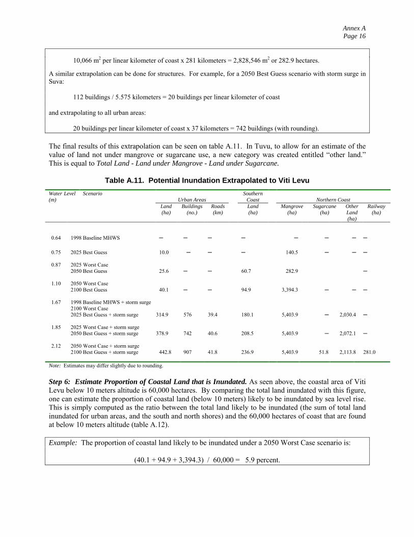
Annex APage 16
10,066 m2 per linear kilometer of coast x 281 kilometers = 2,828,546 m2 or 282.9 hectares.
A similar extrapolation can be done for structures. For example, for a 2050 Best Guess scenario with storm surge inSuva:
112 buildings / 5.575 kilometers = 20 buildings per linear kilometer of coast
and extrapolating to all urban areas:
20 buildings per linear kilometer of coast x 37 kilometers = 742 buildings (with rounding).
The final results of this extrapolation can be seen on table A.11. In Tuvu, to allow for an estimate of thevalue of land not under mangrove or sugarcane use, a new category was created entitled �other land.�This is equal to Total Land - Land under Mangrove - Land under Sugarcane.
Table A.11. Potential Inundation Extrapolated to Viti LevuWater Level(m)
ScenarioUrban Areas
SouthernCoast Northern Coast
Land(ha)
Buildings(no.)
Roads(km)
Land(ha)
Mangrove(ha)
Sugarcane(ha)
OtherLand(ha)
Railway(ha)
0.64 1998 Baseline MHWS ─ ─ ─ ─ ─ ─ ─ ─
0.75 2025 Best Guess 10.0 ─ ─ ─ 140.5 ─ ─ ─
0.87 2025 Worst Case2050 Best Guess 25.6 ─ ─ 60.7 282.9 ─
1.10 2050 Worst Case2100 Best Guess 40.1 ─ ─ 94.9 3,394.3 ─ ─ ─
1.67 1998 Baseline MHWS + storm surge2100 Worst Case2025 Best Guess + storm surge 314.9 576 39.4 180.1 5,403.9 ─ 2,030.4 ─
1.85 2025 Worst Case + storm surge2050 Best Guess + storm surge 378.9 742 40.6 208.5 5,403.9 ─ 2,072.1 ─
2.12 2050 Worst Case + storm surge2100 Best Guess + storm surge 442.8 907 41.8 236.9 5,403.9 51.8 2,113.8 281.0
Note: Estimates may differ slightly due to rounding.
Step 6: Estimate Proportion of Coastal Land that is Inundated. As seen above, the coastal area of VitiLevu below 10 meters altitude is 60,000 hectares. By comparing the total land inundated with this figure,one can estimate the proportion of coastal land (below 10 meters) likely to be inundated by sea level rise.This is simply computed as the ratio between the total land likely to be inundated (the sum of total landinundated for urban areas, and the south and north shores) and the 60,000 hectares of coast that are foundat below 10 meters altitude (table A.12).
Example: The proportion of coastal land likely to be inundated under a 2050 Worst Case scenario is:
(40.1 + 94.9 + 3,394.3) / 60,000 = 5.9 percent.

Annex APage 17
Table A.12 Proportion of Coastal Land Likely to be Inundated by Sea Level Rise
Water Level(m)
Scenario Total Land Area Inundated(in hectares)
UrbanAreas
SouthCoast
NorthCoast
Total VitiLevu
Proportion ofCoastal AreaBelow 10 m
0.64 1998 Baseline MHWS ─ ─ ─ ─
0.75 2025 Best Guess 10.0 ─ 140.7 150.7 0.3%
0.87 2025 Worst Case2050 Best Guess 25.6 60.7 282.9 369.2 0.6%
1.10 2050 Worst Case2100 Best Guess 40.1 94.9 3,394.3 3,529.3 5.9%
1.67 1998 Baseline MHWS + storm surge2100 Worst Case2025 Best Guess + storm surge 314.9 180.1 7,434.4 7,929.4 13.2%
1.85 2025 Worst Case + storm surge2050 Best Guess + storm surge 378.9 208.5 7,476.0 8,063.4 13.4%
2.12 2050 Worst Case + storm surge2100 Best Guess + storm surge 442.8 236.9 7,517.7 8,197.5 13.7%
Note: Total area inundated in north coast equals total area mangrove + total area sugarcane + total other land on table A.11.
B. Economic Impact of Inundation due to Sea Level Rise
This analysis can be done in four major steps:
Step 1: Estimate the economic value of land and structures lost to inundation. The erosion analysisshowed how the economic value of land in the southern coast and land under mangroves could becomputed. For the inundation analysis, additional estimates are needed for land, buildings and roads inurban areas, and sugarcane and railway values in the northern coast.
1.1 Economic Value of Land in Southern Coast. As estimated before, the economic value of land in thesouthern coast of Viti Levu is about US$19,600 per hectare. Because inundation is likely to recur,inundated land is assumed to lose all of its economic value.
1.2 Economic Value of Mangrove Land in Northern Coast. Contrary to coastal erosion, which may lead to areplacement of mangrove species and a net loss, the impact of inundation on mangrove ecosystems islikely to be neutral or even beneficial. Most mangroves should be able to adapt to slow inundation, andthe deeper roots resulting from sea level rise could help trap additional nutrients (Andrew Hooten,personal communication, June 2000). Consequently, no major economic losses resulting frominundation of mangroves are expected, and the inundated mangrove land is costed at US$0 per hectare.
1.3. Economic Value of Urban Land. According to a recent survey conducted by Margaret Chung andconsultations with a major real estate firm in Suva, the value of developed freehold land in the cityaverages about F$40,000 per acre, or F$100,000 per hectare. Assuming that only 9 percent of the land isunder freehold status, and that non-freehold land sells for 20 percent less, the weighted average value ofland is, at 1998 exchange rates (1 US$ = F$1.96):

Annex APage 18
(F$100,000 x 9%) + [0.8 x (F$100,000 x 91%)] = F$81,800 per hectare / 1.96 = US$41,735 per hectare
It is assumed that the market price of urban land reflects its economic value.
1.4. Economic Value of Urban Buildings. The coastal survey in Fiji was conducted just prior to the coup ofMay 2000. Subsequently, it has been difficult to obtain accurate estimates of real estate values.Nonetheless, an estimate made by Robert Gillett (Gillett, personal communication, May 2000), indicatesthe following values for shorefront houses in Suva:
About 1/3 of the houses are of original boxy Indian-style costing approximately F$150,000About 1/3 of the houses have been rebuild, at values of approximately F$250,000About 1/3 of the houses are luxurious dwellings worth about F$400,000 each
For the purpose of the analysis, it is assumed that inundation would destroy about 50 percent of the boxyhouses, 15 percent of the rebuilt houses, and only about 5 percent of the luxury houses (as these aregenerally built to withstand storms). Hence:
(F$150,000 x 50%) + (F$250,000 x 15%) + (F$400,000 x 5 %) = F$132,500 or US$67,600 per building.
This estimate is conservative, since it does not take into account the higher value of commercial buildingsthat could be affected by inundation.
1.5. Economic Value of Urban Roads. According to a JICA proposal (1998), the cost of building a 1.1kilometer of roadway in a residential area in Nadi was F$330,000 in mid-1997. Road construction andimprovements elsewhere were estimated at F$530,000 for 1.5 kilometers of road. These estimatessuggest an average cost of road construction of about F$300-$353,000 per kilometer. Adjusting to 1998values by the housing consumer price index (from IMF reports), yields an estimate of F$314-$361,800per kilometer or US$160-$184,600 per kilometer.
The impact of inundation on roads is difficult to assess. However, discussions with infrastructure expertssuggest that it is not unreasonable to assume a loss of 25 percent of the value of the road, due to the needfor higher maintenance and reconstruction. Hence, the economic value of roads lost to inundation isestimated at:
Average of US$160-$184,600 is US$172,300 x 25 % = US$43,000 per kilometer of road.
1.6. Economic Value of Sugarcane Land in Northern Coast. The economic value of sugarcane land dependson the opportunity cost of the land use, in this case sugarcane plantations. It is assumed that inundatedland would lose all of its sugarcane production value.
The average production of sugarcane ─ accounting for possible reductions in yield due to climate change─ is 52.7 metric tons per hectare per year (FAO 1996 and study estimates). The price of sugarcaneadjusted to 1998 values, was F$75.7 per metric ton. Hence, the value of sugarcane land is:
F$75.7 per metric ton x 52.7 metric tons/ha/year = F$3,987 or US$2,034 per hectare per year.
Similarly to the value of mangrove land in the erosion analysis, it is necessary to compute the futurebenefit stream of sugarcane production lost as a result of inundation. Using a 10 percent discount rate anda benefit stream of 25 years, the present value of sugarcane land is as follows:
Present Value (US$2,034 per year, 25 years, 10% discount rate) = US$18,463 per hectare.

Annex APage 19
1.7. Economic Value of Other Land. A significant amount of land in the northern coast does not fit thedescription of mangrove or sugarcane areas. Unfortunately, no estimates were available of the value ofthis land. Until better estimates are available, the assumption was made that this land was worth 80percent of the agricultural land value in the southern coast (F$5,500 per hectare). Hence, the value of the�other land� lost to erosion is:
F$5,500 per hectare x 80 % = F$4,400 or US$2,200 per hectare
1.8. Economic Value of Railways. No data were available to compute the potential impact of inundationon railways. The railways found in the northern shore are most likely used for sugarcane transport, andare only affected under a 2050 worst case scenario or 2100 best guess scenario with storm surge.
Step 2: Estimate the Economic Value of Land and Structures Lost to Inundation. From the calculationabove, the value of land and structures lost to inundation is as follows:
Unit values of Land and Structures Lost to Inundation:
Urban land US$41,735 per hectareUrban buildings US$67,610 per structureUrban roads US$43,000 per kilometerLand in southern coast US$19,600 per hectareMangrove land in northern coast US$0 per hectareSugarcane land in northern coast US$18,463 per hectareOther land US$2,200 per hectareRailway not computed
These estimates were used to compute the total economic losses due to inundation, by multiplying theunit values by the estimates of land and structures lost on table A.11.
Example:
The urban land lost to inundation under the Best Guess scenario for 2050 is 25.6 hectares. At a value of US$41,735per hectare, the total loss is 25.6 hectares x US$41,735 per hectare = US$1,068,416 or US$1.1 million.
Step 3: Estimate the Total Economic Loss Caused by Climate Change. The next step in the analysis isto estimate the losses that can be attributed to climate change. For this, it is necessary to compare futureconditions with the present baseline. Future conditions with storm surge (SS) need to be compared to theappropriate baseline with storm surge (the second shaded area on table A.13).
Hence, for a 2050 Best Guess (BG) scenario, the economic losses due to climate change are as follows:
Without storm surge: 2050 BG - 1998 Baseline MHWS = US$2.3 millionWith storm surge: 2050 BG with SS - 1998 Baseline with SS = US$76.4-61.8 million = US$14.6 million
The storm surge conditions reflect a 1 in 50 year storm. Assuming conservatively that there is no increasein storm frequency, conditions without storm surge are likely to occur in 49 out of 50 years. Storm surgeconditions would continue to occur in 1 out of 50 years. Hence, the weighted average is:
(US$2.3 million x 49/50) + (US$14.6 million x 1/50) = US$2.5 million

Annex APage 20
Table A.13. Economic Value of Land and Structures Lost to Inundation in Viti Levu(millions of 1998 US$)
Water Level(m)
ScenarioUrban Areas
SouthernCoast
Northern Coast TotalLosses
Land Buildings Roads Land MangroveLand
SugarcaneLand
OtherLand
0.64 1998 Baseline MHWS ─ ─ ─ ─ ─ ─ ─ ─
0.75 2025 Best Guess 0.4 ─ ─ ─ 0.0 ─ ─ 0.4
0.87 2025 Worst Case2050 Best Guess 1.1 ─ ─ 1.2 0.0 2.3
1.10 2050 Worst Case2100 Best Guess 1.7 ─ ─ 1.9 0.0 ─ ─ 3.6
1.67 1998 Baseline MHWS + storm surge2100 Worst Case2025 Best Guess + storm surge 13.1 39.0 1.7 3.5 0.0 ─ 4.5 61.8
1.85 2025 Worst Case + storm surge2050 Best Guess + storm surge 15.8 50.2 1.7 4.1 0.0 ─ 4.6 76.4
2.12 2050 Worst Case + storm surge2100 Best Guess + storm surge 18.5 61.3 1.8 4.6 0.0 1.0 4.7 91.9
Note: Shaded areas indicates baseline values.
For a 2050 Worst Case scenario, the economic losses due to climate change are as follows:
Without storm surge: 2050 Worst Case (WC) - 1998 Baseline MHWS = US$3.6 millionWith storm surge: 2050 WC with SS - 1998 Baseline with SS= US$91.9-61.8 million=US$30.1 million
Weighing the above estimates by the frequency of the storm surge:
(US$3.6 million x 49/50) + (US$30.1 million x 1/50) = US$4.1 million
Step 4: Estimate Annualized Losses Caused by Climate Change. Similarly than for the erosion analysis,the above costs reflect capital losses. In order for the losses to be expressed in annualized terms, it isnecessary to multiply the capital losses by the capital recovery factor of 0.11:
0.11 x US$2.5 million = US$0.28 million
0.11 x US$4.1 million = US$0.45 million
Though the annualized losses (US$0.3-$0.5 million) appear small, it should be remembered that in yearsof strong storm surge, Viti Levu could experience incremental losses in the order of US$14.6-30.1million. If no account is made of current storm impacts, the absolute value of these losses could amountto US$76 to US$92 million by 2050.

Annex APage 21
Impacts of Climate Change on Coral Reefs of Viti Levu
Climate change is expected to affect coral reefs primarily through increases in sea surface temperature(resulting in coral bleaching), sea level rise, and the impact of stronger cyclones and storm surges, whichlead to extensive destruction of the reef system. These impacts need to be computed separately fromthose of land erosion and inundation.
Step 1: Estimate the Total Area of Coral Reefs in Viti Levu. The area of coral reefs surrounding VitiLevu is unknown, though Fiji has about 1 million hectares of reef (WRI 1999). Several approaches arepossible to estimate Viti Levu�s reef area: the first is to assume that Viti Levu�s share of Fiji�s land areaalso applies to its coral reefs. Under this approach, Viti Levu would have 58 percent of Fiji�s reefs, or580,000 hectares. This estimate is clearly exaggerated, however. While Viti Levu is a large island, manyother small islands in Fiji are surrounded by coral reefs, with a ratio of coral reef to land area muchgreater than Viti Levu.
The more correct approach ─ albeit subject to future confirmation ─ is to assume that the area of coralreef is broadly proportioned to the length of the coast line. The total coastal area of Fiji is 5,010kilometers (Robert Gillett, personal communication) while the coastal area of Viti Levu is 750 kilometers,or 15 percent of the total for Fiji. This suggests that the area of coral reefs in Viti Levu is 15 percent ofthat of Fiji, or 150,000 hectares. This estimate was used for the analysis.
Step 2: Determine the Products or Functions Lost as a Result of Climate Change. Climate change islikely to affect the following uses and functions of coral reefs: productivity of subsistence andcommercial fisheries, tourism, biodiversity or habitat values, and coastal protection. The value of thesefunctions is examined in turn below.
As a result to overexploitation and habitat degradation, some 19 percent of Fiji�s coral reefs are presentlyconsidered to be at high risk, with an additional 48 percent are at moderate risk (WRI 1999). As a lowbound estimate, it is assumed that all of the high risk reefs ─ which are already under severe stress ─would die as a result of climate change. As a high end estimate, it is assumed that all of the high riskreefs plus half of the reefs at moderate risk (24 percent) might also die in the future. Thus, the analysisassumes a mortality of 19 to 43 percent of the total area of coral reef. This is a reasonable estimate giventhe latest scientific knowledge and the extent of the bleaching that affected 50-100 percent of the coralsabove 30 meters deep in southern Viti Levu in early 2000 (South and Skelton 2000).
Step 3: Estimate the Economic Losses Resulting from Climate Change
3.1. Annual Losses in Subsistence Fishing. Dead or bleached reefs do not necessarily lose their fisheriesvalue, as they tend to be quickly covered by algae and lead to a proliferation of herbivorous fish. In thelong term, however, dead reefs will tend to break away, and more substantial losses of productivity can beexpected (Clive Wilkinson, Tom Goreau, and Herman Cesar, personal communication, May 2000). It isassumed conservatively that the 19-43 percent of reefs that would die would lose 50 percent of theirfisheries value.
Though Viti Levu may have only 15 percent of the Fiji reefs, the majority of the artisanal and subsistencecatch originates from the island, where 77 percent of the Fiji population live. Hence, it is reasonable toassume that the subsistence fisheries of Viti Levu account for 15 to 77 percent of Fiji�s total.
As seen in the estimation of mangrove values, subsistence fishing in Fiji was valued at approximatelyF$53.5 million in 1998, taking into account 1998 official estimates of subsistence catch and the average

Annex APage 22
market price for artisanal fisheries (FFD 1999). Coral reefs are assumed to account for between 35 and45 percent of the coastal fisheries production (Esaroma Ledua, personal communication, March 2000).
The value of subsistence fishing in Viti Levu is therefore:
F$53.5 million x 15 to 77 % x 35 to 45 % = F$2.8 to F$18.5 million
(total value of subsistence (Viti Levu’s share of (Share of subsistence fisheries) ( total catch) (fisheries dependent on coral reefs)
Assuming a 19 to 43 percent loss in reefs due to climate change, and a loss of 50 percent in reef fisheriesproductivity, the impacts of climate change on Viti Levu�s subsistence fisheries are as follows:
F$2.8 to F$18.5 million x 19 to 43% x 50% = F$0.3 to F$4.0 million per year(Value of subsistence fishing (Estimated reef (loss of fisheries in Viti Levu) mortality due to from dead reefs)
climate change)
3.2. Annual Losses in Commercial Fishing. As per the estimation of mangrove values, artisanal fishing inFiji was valued at F$20.7 million in 1998 (FFD 1999). Using the same assumptions as for subsistencefishing:
F$20.7 million x 15 to 77 % x 35 to 45 % = F$1.1 to F$7.2 million(total value of artisanal (Viti Levu’s share of (Share of artisanal fisheries) ( total catch) (fisheries dependent on coral reefs)
F$1.1 to F$7.2 million x 19 to 43% x 50% = F$0.1 to F$1.5 million per year(Value of artisanal fishing (Estimated reef (loss of fisheries in Viti Levu) mortality due to from dead reefs)
climate change)
3.3. Annual Losses in Tourism. While tourism is a F$568 million a year industry in Fiji, only a relativelyminor proportion of tourists is likely to cease visitation due to coral reef mortality. A similar phenomenawas reported in Maldives after the massive reef mortality in 1997-98. Most tourists were said to visit theMaldives for its beaches and leisure, rather than its reefs. The strange coloration of bleached reefs, andthe growth of soft coral and herbivorous fish can in some cases provide additional attractions forsnorkelers and divers.
The most likely tourist category to be affected by coral reef mortality are dive tourists. Numerousattempts were made to obtain statistics on dive tourism in Fiji, but these data does not appear to beavailable. Pending further information, it is assumed that extensive coral reef mortality would result in a15 percent drop in tourism revenues. This is in line with recent estimates from Palau that indicate a 9percent drop in divers� willingness to pay following the 1997-98 bleaching event (Graham, Idechong andSherwood 2000). Similar surveys in East Africa indicate that 19 percent of the tourists visiting Zanzibar(and 39 percent of those visiting Monbasa) would likely reroute their travel if they knew coral reefs werebleached (Westmacott, Cesar and Pet Soede 2000).
It was similarly difficult to ascertain the share of tourism revenues that is spent on Viti Levu. Aconservative assumption is to use Viti Levu�s share of Fiji�s land mass (58 percent). The impact ofclimate change on tourism linked to the health of coral reefs is therefore:
F$568 million x 58% x 15% = F$49.4 million(annual tourism revenues) (% of tourists to Viti Levu) (proportion of tourism
likely to be affected by coral mortality)

Annex APage 23
F$49.4 million x 19 to 43% of the reefs = F$9.4 to F$21.2 million per year
(tourism revenues in Viti (estimated coral mortalityLevu likely to be affected by from climate change)coral mortality)
3.4. Annual Losses in Habitat Value. In addition to their fisheries, recreational and protection values, coralreefs play important roles in biodiversity as habitats for marine life. No estimate is available for thisfunction in Fiji. However, a parallel study for the Galapagos indicates a value (expressed in 1998 F$) ofabout F$16 per hectare (de Groot 1992). This estimate is used as here as a fist order approximation only.
As discussed above, Viti Levu is assumed to have 15 percent of Fiji�s reefs. Hence, the habitat valuelikely to be lost to climate change would be as follows:
F$16 per hectare per year x 150,000 hectares x 19 to 43 % = F$0.5 to F$1.0 million per year
(annual habitat value) (estimated area of Viti (estimated coral Levu’s reefs) mortality from
climate change)
3.5. Annual Losses in Coastal Protection Value. Coral reefs play a vital role in the protection of the coast.Following bleaching or mortality events due to elevations in ocean surface temperature, coral reefs arelikely to sustain their production function for some time, but will eventually break and wash away (CliveWilkinson, personal communication). While the loss of coastal protection caused by bleaching events istechnically separate from the impact of sea level rise on coastal areas, it is difficult to isolate the twoimpacts. Hence, no estimate was done of the loss of coastal protection resulting from coral reef mortality.Estimates from other countries indicate that this value may be substantial, around US$60,000 toUS$550,000 per square kilometer of reef (Cesar 1996).
Step 4: Add up the Impacts. Since the estimates of the various impacts are already annualized, no furtheradjustment is required, as done for the erosion and inundation analyses. Hence, the impacts can be simplyadded to give an estimate of the impacts of climate change on the coral reefs of Viti Levu (table A.14).
Table A.14. Total Estimated Annual Economic Impact of Climate Change on theCoral Reefs of Viti Levu, Fiji
(millions of 1998 US$)
Losses in: Annual Damages
Millions of 1998 F$ Millions of 1998 US$
Subsistence fisheries 0.3 to 0.4 0.1 to 2.0 Commercial (coastal) fisheries 0.1 to 1.5 0.05 to 0.8Tourism 9.4 to 21.2 4.8 to 10.8Habitat 0.5 to 1.0 0.2 to 0.5Coastal Protection ─ ─Others (nonuse values, etc.) + +
Total estimated damages 10.3 to 27.7 5.2 to 14.1
Notes: ─ Not available; + Not available, but believed to be substantial.

Annex APage 24
Tarawa Atoll
Impact of Erosion Caused by Climate Change on Tarawa’s Coast
A. Physical Impact of Coastal Erosion due to Sea Level Rise
The Tarawa atoll has a land area of 30 square kilometers (about 3,000 hectares). All land in Tarawa canbe classified as �coastal� since it rarely rises more than 5.0 meters above sea level, with much of the landat less than 3 meters altitude (McLean 1989).
To model the impact of erosion and inundation, two case study sites were selected: Bikenibeu island,representing the type of conditions found in South Tarawa, and Buariki, representing the conditions foundin North Tarawa. Two transects were surveyed in Bikenibeu and three transects were surveyed in Buariki(table A.15).
Table A. 15. Case Study Sites for TarawaCoastal Type Area
(hectares)Proportion ofTarawa atoll
Case StudySites
Area of CaseStudy Sites (hectares)
South Tarawa; densely populated, some coastal protection,location of major infrastructure and government 1,577 50% Bikenibeu 104
North Tarawa: sparsely populated, less developedinfrastructure, traditional dwellings, subsistence living 1,526 50% Buariki 293
Notes: Area of South Tarawa and North Tarawa said to be 3,896 and 3,771 acres, respectively, in the study�s economic analysisreport. Area of Bikenibeu and Buariki derived from table 3.10 of the original Kiribati Vulnerability and Adaptation report.
The estimate of physical impact involved three major steps:
Step 1. Estimate Potential Shoreline Erosion. The level of shoreline displacement was estimated usingthe Shoreline Translation Model (STM) described earlier in this Annex, and is shown on table A.16.
Table A. 16. Protential Shoreline Retreat in Case Study Sites, TarawaProjected Area of Buariki Eroded Projected Area of Bikenibeu ErodedSea Level
Rise(meters) North Transect Central Transect South Transect West Transect East Transect
ShoreRetreat(meters)
AreaEroded(hectares)
ShoreRetreat(meters)
AreaEroded(hectares)
ShoreRetreat(meters)
AreaEroded(hectares)
ShoreRetreat(meters)
AreaEroded(hectares)
ShoreRetreat(meters)
AreaEroded(hectares)
0.1 0.6 0.1 0.9 0.2 0.5 0.1 0.5 0.2 0.4 0.20.2 1.2 0.2 2.3 0.5 1.0 0.2 1.0 0.4 0.6 0.20.3 2.6 0.4 3.0 0.7 2.3 0.4 2.0 0.8 0.8 0.30.4 3.2 0.5 4.4 1.0 2.9 0.5 2.5 1.0 1.0 0.40.5 4.5 0.7 5.0 1.1 3.6 0.6 3.5 1.4 1.2 0.50.6 5.2 0.8 6.5 1.4 4.2 0.7 4.0 1.6 1.5 0.60.7 6.5 1.0 7.3 1.6 4.8 0.8 5.0 2.0 1.8 0.70.8 7.2 1.2 9.1 2.0 5.5 0.9 5.5 2.2 2.2 0.90.9 8.4 1.3 14.2 3.1 6.1 1.0 6.5 2.6 2.7 1.11.0 9.5 1.5 30.5 6.7 6.7 1.1 7.0 2.8 3.2 1.3
Notes: Shaded areas indicate the scenarios of sea level rise considered in the study

Annex APage 25
Step 2. Estimate the Proportion of the Study Sites Land that is Lost to Erosion. To compute theproportion of the study sites� land that is likely to be lost to erosion, the projected area eroded in each ofthe transects was first added up to provide a total area eroded for Buariki and Bikernibeu.
Example: For a 0.5 meters sea level rise, the area eroded in Buariki is as follows:
0.7 hectares + 1.1 hectares + 0.6 hectares = 2.4 hectares(north transect) (central transect) (south transect)
For a 0.4 meters sea level rise, the area eroded in Bikenibeu is:
1.0 hectares + 0.4 hectares = 1.4 hectares (west transect) (east transect)
These totals can then be compared with the area of the study sites (table A.15) to determine the proportionof land lost to erosion.
Example: For a 0.5 meters sea level ride in Buariki:
2.4 hectares / 293 hectares = 0.0082 or 0.8 percent.
For a 0.4 meters sea level rise in Bikenibeu:
1.4 hectares / 104 hectares = 0.013 or 1.3 percent.
The proportion of land eroded for all major sea level rise scenarios is shown on table A.17.
Table A.17. Estimated Potential Land Erosion as a Result of Climate Change in TarawaAreas 2025 2050 2100
Estimate Best guess Worst case Best guess Worst case Best guess Worst caseSea level rise 0.1 0.2 0.2 0.4 0.5 1.0
NorthTarawa
Potential land eroded in Buariki (in hectares)
0.4 0.9 0.9 2.0 2.4 9.4
Percentage of total land (%) 0.1 0.3 0.3 0.7 0.8 3.2Extrapolated land eroded in North Tarawa (in hectares) 2.0 4.6 4.6 10.2 12.7 48.8Value of eroded land (in US$ million) 0.1 0.2 0.2 0.4 0.6 2.1
SouthTarawa
Potential land eroded in Bikenibeu (in hectares) 0.4 0.6 0.6 1.4 1.9 4.1Percentage of total land (%) 0.4 0.6 0.6 1.3 1.8 3.9Extrapolated land eroded in South Tarawa (in hectares) 5.7 9.8 9.6 21.1 28.5 61.8Value of eroded land (in US$ million) 0.3 0.6 0.6 1.3 1.7 3.7
Total Tarawa 0.4 0.8 0.8 1.7 2.3 5.8
Shaded areas refer to the example given above. Numbers may not add up due to rounding.

Annex APage 26
Step 3. Extrapolate Erosion to the Rest of Tarawa. If it can be assumed that Buariki and Bikenibeu arebroadly representative of the conditions found in North and South Tarawa, then the proportions of landlost to erosion can also be applied to the total area of North and South Tarawa to determine the totalpotential land eroded in the atoll.
Example:
For 0.5 meters sea level rise in North Tarawa:
0.83 percent x 1,526 hectares = 12.7 hectares
(proportion of land lost (area of North Tarawa) to erosion in Buariki)
For 0.4 meters sea level rise in South Tarawa:
1.34 percent x 1,577 hectares = 21.1 hectares
These estimates are shown on table A.17 above.
B. Economic Impact of Coastal Erosion due to Sea Level Rise
The analysis of economic impacts involved two key steps:
Step 1: Estimate the Economic Value of Land Lost to Erosion. To compute the economic impact ofcoastal erosion, it is necessary to know the value of land per hectare. The Land Management Division inKiribati quotes the following values for land in Tarawa:
For North Tarawa: Unimproved residential land A$18,000 per acreCommercial land: A$100,000 per acre
For South Tarawa: Unimproved residential land: A$20,000 per acreCommercial land: A$100,000 per acre
For the purposes of the estimation, and by lack of other data, it was assumed that these values reflect theeconomic value of land in Tarawa.
In North Tarawa, it was assumed that 10 percent of the land was used for commercial purposes, while 90percent was assumed to be unimproved residential land. In South Tarawa, 20 percent of the land wasassumed to be for commercial purposes, while 80 percent was unimproved residential land. Hence, theweighted average value of land is:
For North Tarawa: (A$18,000 x 90%) + (A$100,000 x 10%) = A$26,200 per acre
For South Tarawa: (A$20,000 x 80%) + (A$100,000 x 20%) = A$36,000 per acre
Converting into hectares (1 hectare = 2.5 acres) and US$ (1US$ = A$1.5 in 1998):
For North Tarawa: A$26,200 x 2.5 / 1.5 = US$43,670 per hectareFor South Tarawa: A$36,000 x 2.5 / 1.5 = US$60,000 per hectare
These unit costs can then be applied to the extrapolated land eroded in North and South Tarawa (tableA.17) to determine the potential losses due to erosion.

Annex APage 27
Example:
For the worst case scenario of 2100, the estimated land eroded in North Tarawa is 49.3 hectares. The eroded land inSouth Tarawa is 60.6 hectares. Applying the unit costs above:
For North Tarawa: 48,8 hectares x US$43,670 per hectare = US$2,131,096 or US$2.1 millionFor South Tarawa: 61.8 hectares x US$60,000 per hectare = US$3,708,000 or US$3.7 million
The total value of land eroded in Tarawa for this scenario is US$5.8 million.
The economic costs of erosion are therefore US$0.4-$0.8 million in 2025, US$0.8-$1.7 million in 2050,and US$2.3-$5.8 in 2100.
Step 2: Estimate the Annualized Value of the Losses. The values above represent the loss of capital dueto inundation. To calculate the annualized losses, it was assumed, in discussions with an expert, that theduration of most structures in Tarawa averaged about 10 years. Using a discount rate of 10 percent, andapplying it to the capital recovery factor formula gives the following capital recovery factor:
[i(1+i)n] / [(1+i)n -1] where i = rate of interest (10 percent) and n = number of years when losses can accrue (10 years).
Hence, [i(1+i)n] / [(1+i)n -1] = [0.1(1.1)10] / [(1.1)10 -1] = 0.16
Applying this factor to the capital losses due to erosion, yields the following annualized losses:
0.16 x US$0.4 to $0.8 million = US$0.1-$0.13 million in 20250.16 x US$0.8 to $1.7 million = US$0.1-$0.3 million in 20500.16 x US$2.3 to $5.8 million = US$0.4-$0.9 million in 2100
Impact of Inundation Caused by Climate Change on Tarawa’s Coast
A. Physical Impact of Inundation due to Sea Level Rise
The analysis of physical impacts involved four key steps:
Step 1: Determine Baseline Conditions. The Mean High Water Spring (MHWS) tide level for Tarawa is2.53 meters. A 1 in 14 year storm ─ the baseline with storm surge ─ raises the sea level toapproximately 3.0 meters under baseline conditions.
Step 2: Estimate Projected Changes in Water Level under Sea Level Rise. The water levels for thedifferent sea level rise scenarios are displayed on the first column of table A.18. These are derived bysimply adding sea level rise scenarios onto the MHWS baseline.
Step 3: Estimate the Area of Inundated Land and Infrastructure. Based on the simulations of the areainundated at various water levels, the land area, number of structures, and length of road inundated werecalculated from maps provided by the Kiribati Land Management Division. The results are presented ontable A.18.

Annex APage 28
Table A.18. Potential Inundation at Case Study Sites, Tarawa
Note: Projected losses in structures and roads derived from topographic maps (Land Management Division of Kiribati). Stormsurge is based on a 1 in 14 year event (Solomon 1997). Figures in parenthesis indicate percentage of the land, infrastructureand/or roads inundated (relative to the total for the study sites).
Step 4: Extrapolate to all Tarawa. Assuming that Buariki and Bikenibeu are broadly representative ofthe conditions of North and South Tarawa, respectively, a simple extrapolation can be used to derive thephysical impact on the entire atoll. For land, the percentage of land that is projected to be inundated inBuariki and Bikenibeu was applied directoy to the area of North and South Tarawa. For example, for the2025 Worst Case scenario, 18 percent of the land of Buariki is expected to be inundated. This percentagecan be then applied to the total area of North Tarawa, 1,526 hectares (table A.15), yielding a total area ofland inundated of approximately 275 hectares (table A.19).
Similarly for structures, a simple extrapolation can be used. To calculate the number of structures forNorth Tarawa under a 2025 Worst Case scenario:
No. of structures affected in Buariki (196) x Area of North Tarawa (1,526)/Area of Buariki (293) = 1,021 structures.
The results are summarized on table A.19, which also contains the results of the economic analysisexplained below.
B. Economic Impact of Inundation due to Sea Level Rise
The economic impact analysis involved three key steps:
Step 1: Estimate the economic value of land and structures lost to inundation. From the economicanalysis of erosion impacts, the average unit value of land in South Tarawa was estimated at US$60,000per hectare, while the value of land in North Tarawa averaged US$43,670 per hectare.
Buariki BikenibeuWater Level
(m)Scenario: Land area
affected(hectares)
Structures(number)
Roads(kilometer)
Land areaaffected(hectares)
Structures(number)
Roads(kilometer)
2.53 1998 Baseline MHWS -- -- -- -- -- --
2.75 2025 Worst Case2025 Best Guess
53 (18%) 196 (59%) 6.55 (77%) 0 (0%) 0 0
3.00 1998 Baseline with storm surge2050 Worst Case2100 Best Guess
89 (30%) 213 (64%) 6.55 (77%) 1.9 (2%) 34 ( 2%) 0
3.2 2050 Best Guess + storm surge 161(55%) 229 (69%) 7.5 (89%) (25%) 423 (27%) 1.26 (29%)
3.56 2050 Worst Case +storm surge2100 Best Guess+storm surge
2100 Worst Case
233 (80%) 245 (74%) 8.5 (100%) 56 (54%) 986 (63%) 2.83 ( 66%)
4.0 2100 Worst Case+ storm surge 248 (85%) 316 (95%) 8.5 (100%) 83 (80%) 1302 (84%) 4.36 (100%)

Annex APage 29
Table A.19. Estimated Economic Value of Land and Structures Lost to InundationWater Level(m) Scenario
North Tarawa South Tarawa TotalTarawa
Land Lost Structures Lost Land Lost Structures Losthectares Costs
(US$M)No. Costs
(US$M)Hectare
sCosts
(US$M)No. Costs
(US$M)Costs
(US$M)
2.53 1998 Baseline MHWS ─ ─- ─- ─- ─- ── ─- ── ──
2.75 2025 Worst Case2050 Best Guess 274.7 12.0 1,021 20.4 0.0 0.0 0.0 0.0 32.4
3.00 1998 Baseline + storm surge2050 Worst Case2100 Best Guess 457.8 20.0 1,109 22.2 31.5 1.9 516 10.3 54.4
3.2 2050 Best Guess + storm surge 839.3 36.7 1,193 23.9 394.3 23.7 6,414 128.3 212.4
3.56 2050 Worst Case + storm surge2100 Best Guess + storm surge
2100 Worst Case 1,220.8 53.3 1,276 25.5 851.6 51.1 14,951 299.0 429.0
4.0 2100 Worst Case + storm surge 1,297.1 56.6 1,646 32.9 1,261.6 75.7 19,743 394.9 560.1
Shaded area indicates baseline conditions.
The cost of structures was estimated at A$30,000 each (US$20,000), from data from the Kiribati LandManagement Division. Table A.19 shows the estimate of economic value of land and structures lost toinundation. The interpretation of the topographic maps did not allow for a differentiation of the type ofstructure affected. Data were also not available to estimate the economic costs of road losses to erosion.
Example: In the 2050 Best Guess Scenario, about 1,021 structures are estimated to be affected by inundation. Thevalue of these losses is therefore:
1,021 x US$20,000 or US$20.4 million.
Step 3: Estimate the Net Economic Losses Caused by Climate Change. Similarly to the Viti Levuanalysis, the future conditions need to be compared with the correct baseline: for example, if one isestimating conditions under 2050 Best Guess with storm surge, the correct comparator would be ascenario of 1998 Baseline conditions with storm surge.
Hence, for a 2050 Best Guess (BG) scenario, the economic losses are as follows:
Without storm surge: 2050 BG - 1998 Baseline MHWS = US$32.4 millionWith storm surge: 2050 BG with SS - 1998 Baseline with SS = US$212.4 - US$54.4 = US$158.0 million
The storm conditions reflect a 1 in 14 year storm. Assuming no change in the frequency of storms, stormsurge conditions are likely to occur once every 14 years, while no storm surge conditions are likely tooccur in 13 out of 14 years. The weighted average loss is therefore:
(US$32.4 million x 13/14) + (US$158.0 million x 1/14) = US$41.4 million
For a 2050 Worst Case Scenario (WC), the economic losses would be:
Without storm surge: 2050 WC - 1998 Baseline MHWS= US$54.4 millionWith storm surge: 2050 WC with SS - 1998 Baseline with SS = US$429.0 - US$54.4 = US$374.6 million
(US$54.4 million x 13/14) + (US$374.6 million x 1/14) = US$77.3 million

Annex APage 30
Step 4: Estimate the Annualized Losses Caused by Climate Change. Similarly than for the erosionanalysis, the costs above reflect capital losses. For the losses to be expressed in annualized terms, it isnecessary to multiply them by the capital recovery factor, which is 0.16 (see erosion analysis).
The annualized costs are therefore:
0.16 x US$ 41.4 million = US$6.6 million for a best guess scenario in 2050
0.16 x US$ 77.3 million = US$12.4 million for a worst-case scenario in 2050.
In years of strong storm surge, Tarawa could experience incremental losses in the order of US$158-$375million by mid-century. If no account is made of current storm impacts, the absolute value of these lossescould amount to US$212-$429 million by 2050.
Impacts on Coral Reefs and Mangroves
Tarawa has lost some 70 percent of its mangroves since 1940, and only 57 hectares remain (Metz 1996).The impact of sea level rise is therefore considered to be negligible, and could be even positive as higherwater levels may lead to denser root systems and expansion of mangroves shoreward.
Climate change is likely to have a significant impact on coral reefs, however. Bleaching caused bywarmer sea surface temperatures and the impact of sea level rise could impact subsistence andcommercial fisheries, habitat functions, and the coastal protection role of coral reefs. Losses in tourismvalue are considered negligible as Tarawa does not have a developed dive or snorkel tourism industry.
The physical and economic impact analysis involved three major steps:
Step 1: Estimate the Area of Coral Reefs: The reef area of Tarawa is 129 km2 or 12,900 hectares(Stratus 2000).
Step 2: Determine the Products or Functions Lost as a Result of Climate Change. No estimate isknown of the present status of coral reefs in Tarawa. However, in-country discussions indicate that it isnot unreasonable to assume a loss of 10 to 40 percent of the reefs by 2050 under climate changeconditions. Similarly to Viti Levu, it is assumed ─ conservatively ─that dead reefs would retain about 50percent of their fisheries productivity.
Step 3: Estimate the Economic Losses Resulting from Climate Change
3.1. Annual Value of Subsistence Fishing. Government statistics put the value of subsistence fishing inKiribati at A$6.3 million in 1998. This figure needs to be adjusted for Tarawa. A population proportion(45 percent of the I-Kiribati population lives in Tarawa) rather than an area adjustment was used becauseseveral of the islands of Kiribati ─ particularly on the Phoenix group ─ are uninhabited.
Hence, A$6.3 x 45 % = A$2.8 million (for 12,900 hectares of reefs)
Assuming a 10 to 40 percent reef loss, and a 50 percent loss in fisheries productivity, the value ofsubsistence fisheries lost is:

Annex APage 31
0.10 to 0.40 x 0.5 x A$2.8 = A$0.14 to $0.57 million, or (at an exchange rate of 1 US$ = A$1.5)
US$0.14 to $0.38 million per year
3.2. Annual Value of Commercial Fishing. Commercial fishing in Kiribati is targeted primarily at offshoretuna resources which are not directly related to coral reefs. The value of commercial reef fisheries, whichare commonly designated as �artisanal fisheries�, is unknown in Kiribati. However, exports ofornamental fish and seaweed were valued at A$0.7 million each in 1998, in accordance with IMFstatistics. This almost certainly underestimates commercial fish production, but it is difficult to separateoffshore tuna from reef-related fisheries in the fish export category found in official statistics. Hence,only ornamental fish and seaweed value were taken into account in the analysis:
A$0.7 million (for seaweed) + A$0.7 million (for ornamental fish) = A$1.4 million
Adjusting for Tarawa and for reef loss gives the following economic value of commercial reef fisherieslost to climate change:
0.10 to 0.40 x 0.5 x 45% x A$1.4 million = A$0.032 to A$0.126 or US$0.02- $0.08 million per year
3.3 Annual Habitat Value. A study in the Galapagos (de Groot 1992) estimates the annual habitat value ofcoral reefs at approximately US$8 per hectare of reef. However, the conditions in the Galapagos are toodistinct from those in Kiribati for this estimate to be of relevance. The habitat value of coral reefs inTarawa is probably substantial, but it was not quantified by the study.
3.4. Coastal Protection Value. Given the difficulties of separating the impacts of coral reef loss from thoseof inundation and erosion resulting from sea level rise, the coastal protection value of coral reefs wasassumed to be largely accounted for in the erosion and inundation analysis, and was therefore notquantified here.
Hence, the annual value of coral reefs lost due to climate change in the Tarawa atoll is estimated atUS$0.16 to $0.46 million per year.

Annex APage 32
C. Impacts on Water Resources
For the estimation of the impacts of climate change on water resources in Viti Levu and Tarawa, the studyteam followed slightly different methodologies. In Viti Levu, where cyclones are of paramountimportance, historical records of these extreme events were used to derive an estimate of the futureimpact. The impact on climate change on surface hydrology was based on the water resources modeldeveloped by PACCLIM. The Tarawa water resources analysis, however, used a SUTRA groundwatermodel (Voss 1984) which took into account the mixing between freshwater and underlying seawater.This is considered superior and of greater reliability than the �sharp interface� model incorporated intoPACCLIM, which assumes a sharp boundary between freshwater and seawater. The specific methodsfollowed in the two case studies are outlined in further detail below.
Viti Levu
The impacts of climate change on the water resources of Viti Levu were estimated for cyclones, surfacehydrology and water balance. No estimate of incremental costs could be made for El Niño-relateddroughts, however, given the absence of data on baseline drought conditions. Nonetheless, the impacts ofdroughts is partially taken into account by the agriculture impact analysis (Section D).
Impact of More Intense Cyclones
Fiji has the highest incidence of cyclones in the South Pacific, an average of 1.1 cyclones a year (Pahalaland Gawander 1999). To be as representative as possible of present-day conditions, the intensity andfrequency of actual cyclones in the 1992-99 period was used as a baseline. Reliance on historical datawas necessary since GCM models and PACCLIM do not reflect well the effects of cyclones. The impactanalysis involved three key steps.
Step 1: Estimate the Future Impact of Cyclones. Jones and others (1999) estimate that cyclone intensity(maximum wind speed) could increase by 0-20 percent by mid-century as a result of climate change. Inorder to compute the potential impacts of this increase in intensity, it was necessary to estimate how theincrease in wind speed will affect cyclone damage.
Three estimates were used for this purpose:
• The historical records of the Fiji Meteorological Services for seven recent (1983-97) cyclonesindicate damages of F$67 million (in 1998 value) for an average cyclone with wind speed of 58knots. A 20 percent increase in wind speed over this historical average would be equivalent tocyclones Oscar (68 knots, 1983) and Eric (72 knots, 1985), which averaged F$106 million indamages ─ a 59 percent increase (see figure A.3).
• From the existing theory, an increase in wind speed by 20 percent should result in a 44 percentincrease (1+0.2)2 = 1.44 in wind force (J. Terry, personal communication, May 2000).
• A recent study (Clark 1997) indicates that a 15 percent increase in cyclone severity is likely to resultin a doubling of the damages, or a 100 percent increase.

Annex APage 33
Figure A.3. Cyclone Damage as a Function of Wind Speed, FijiData courtesy from Fiji Meteorological Services.
Taking these three estimates into consideration, an increase in wind speed of 20 percent could result in a44 to 100 increase in total damages. This broad estimate recognizes the large variations that can resultfrom cyclone origin, trajectory and characteristics.
Step 2: Estimate the Baseline Conditions. Using the 1992-99period as an analogue for baseline conditions, the averageannual damages due to cyclones amount to F$28.3 million peryear in 1998 values (table A.20).
The Fiji Meteorological Services confirmed that the estimateddamages pertain to Fiji as a whole, and not just to Viti Levu.Given the correlation between population concentration andinfrastructure, adjusting the damages by the proportion of thepopulation that lives in Viti Levu is preferable to adjusting itby area. Hence, the average annual cyclone damages for VitiLevu ─ the baseline for the analysis ─ is:
F$28.3 million per year x 77 % = F$21.8 million per year
Table A.20. Damages from Cyclones in Fiji(1992-99)
Cyclone Year Damages(millions of 1998 F$)
Joni 1992 2Kina 1993 188Gavin 1997 35Gale June 1997 1
AverageYearly average 1992-99 (8 years)
56.5
28.3
Source: Fiji Meteorological Services, and backgroundstudies to this report.
Maximum Cyclone damageWind Speed (F$ million)
Oscar (1983) 68 148 Average cycloneEric (1985) 72 64 Wind Speed DamagesGavin (1985) 42 2 58 67Sina (1990) 54 33Joni (1992) 55 2 Average cyclone + 20%Kina (1993) 60 188 Wind Speed DamagesGavin (1997) 56 35 70 106
Relationship Between Maximum Wind Speed and Damages for Major Cyclones in Fiji (1983-1997)
Storm Gavin (1985) Joni (1992)
Sina (1990) Gavin (1997)
Eric (1985)
Oscar (1983)
Kina (1993)
0
40
80
120
160
200
0 10 20 30 40 50 60 70 80
Maximum Wind Speed (knots)
Dam
ages
(199
8 F$
mill
ion)
Source: Fiji Meteorological Services.. Damages are converted to 1998 costs

Annex APage 34
Step 3: Estimate the Future Economic Costs of a Rise in Cyclone Intensity. The impact of a 0 to 20percent increase in maximum cyclone intensity is as follows:
• If the change is 0 percent, climate change has zero incremental impact;• If the change is 20 percent, damages could increase by 44 to 100 percent
Thus, for a 20 percent increase in cyclone intensity:
44 % to 100 % of F$21.8 million = F$9.6 to F$21.8 million , or US$4.9-$11.1 million at 1998 exchange rates.
Hence, the average annual incrementalimpact of climate change on cycloneintensity is US$0 to US$11.1 million.
However, in absolute (non incremental)terms, the likely cost of an extreme eventin Viti Levu would be:
F$56.5 million x 0.77 = F$43.5 (Average cyclone (CorrectionLosses in 92-99) for Viti Levu)
F$43.5 million / 1.96 x 0-2.0 =(Losses in (US$ (ProjectedViti Levu) conversion) increase in
intensity)
= US$0-$44 million
Impact of Droughts
With El Niño conditions expected toprevail in the future, Fiji could experienceaccentuated droughts. The 1997-98 droughtwhich caused damages of F$275 to F$325million could well become the norm in thefuture. The drought affected food supplies,commercial crops, livestock, and the watersupply of schools and communities (tableA. 21). The damages of the 1997/98drought ─ a 1 in 100 years event ─ areconsidered indicative of the type ofdroughts that might be expected in thefuture. Since approximately F$125million were losses to sugarcane (mostlyincurred in Viti Levu) and F$15 millionwere losses to other crops, one can assumethe following indicative (absolute) costs forfuture droughts in Viti Levu:
Table A.21. Major Drought-Related Damages andExpenditures for the Drought of 1997-1998, Fiji
(millions of 1998 F$)
Item Cost$125
Sugarcane crop rehabilitation programme $43.7Food and water rations $33a
Weaning foods $3.6 b
Food crop losses $15 c
Crop re-establishment needs $0.41Welfare payments & lost income $75d
School children funding $0.625 e
School water tanks and gardens $1.5Draft animals grass-starved $2.4 f
Milk production decline (50%) $10.9g
Farm drains and creeks $0.26 h
Irrigation to re-establish sugarcane $0.040Boreholes for water supply $0.630 i
Commercial forest $80 j
Health and nutrition $1.8 k
Macro impacts + l
Fire damage (up to 10% of forest areas) +Tourism +
Total F$313.9+Notes:a. Ten months at $3.3 million per month.b. F$360,000 per month times 10 months.c. Estimate of revenue losses from failed new plantings, by Director of AgExtension.d. F$2,000 per family times 15,000 farm families, covering 6 months ofrecovery, prorated to also include 9 months of zero income. There is somepotential double counting with the sugarcane crop loss value on line 1.e. 10,000 children missed school because of hardship. F$500K wasfundraising target to reach 8,000 still in need.f. Molasses block feeding program to restore work animals to work condition.g. F$39,600 loss per day, for 275 days (75% of a year).h. One year of 2 year grant program to clean up drains.i. 675 families served by boreholes, at F$937 per family.j. Re-establish dead plants only, only for mahogany plantation.k. Foreign aid food assistance received.l. Budget deficit of 2.4% GDP; negative GDP growth of 4.0% rather thananticipated 3.0% positive growth. Cost to government is 30% of budget (or 3times the revenue loss).
Source: UNDAC (1998) supplemented with original analysis.

Annex APage 35
The total costs, F$275─$325 million, are equivalent to US$140─$165 million
The agricultural losses, F$125 + F$15 million are equivalent to US$71 million
Thus, the non-croped related losses in Viti Levu are:
(US$140─$165 million) � US$71 million = US$69─$94 million x 0.77 = US$50-$70 million(rounded)
The crop related losses in Viti Levu include all the losses of sugarcane plus 77 percent of the losses inother crops:
US$64 million + (US$7.7 million x 0.77) = US$70 million
From 1983 to 1998, Fiji experienced four El Niño related droughts, or 1 every 4 years. With theexception of the 1997-98 event, these more normal droughts could be considered the baseline variabilityconditions against which to measure a more severe event (such as the 1997-98 drought). Unfortunately,no information exists on the impact of these earlier droughts apart from agricultural yields, and onecannot rule out the possibility that the 1983-98 period already reflects some incremental impacts ofclimate change. Given these constraints, the incremental impact of climate change on droughts could notbe assessed at this stage. About 40-50 percent of the costs of the 1997-98 drought involve agriculturalimpacts, and these were assessed separately in Section D.
Impact of Changes in Precipitation and Temperature on River Flow
The impact of rainfall changes on the water resources of Viti Levu was estimated for two water courses,the Nakauvadra Creek and the Teidamu Creek. The Nakauvadra Creek drains 28 km2 of steeplands innorthern Viti Levu. The Teidamu Creek drains a 56 km2 watershed in the northwestern part of Viti Levu.Both streams have been monitored by the Hydrology Section of the Fiji Public Works Department sincethe early 1980s.
Projections of rainfall for Fiji under climate change conditions vary according to the two GCM modelsused by the study, which predict both an increase (with the CSIRO9M2 model) and a decrease in rainfall(DKRZ model). Using the PACCLIM water resources impact model, the results suggest that under thescenarios of climate change considered by the study, there would be a change of ± 10 % in the waterflow by 2050 and of ± 20 % by 2100 (table A.22). Given the similar climate, land uses, topography andcommercial areas between these creeks and the major Nadi and Ba rivers, similar changes in flow mayoccur there. A possible increase of 10-20% in flood volume could cause extensive damage to industrialand commercial areas. Conversely, if a lower rainfall scenario materializes, the Nadi, Ba and Sigatokarivers could experience salt intrusion causing problems for agricultural irrigation.
The economic impact of these scenarios could not be assessed due to lack of data.

Annex APage 36
Table A.22 Predicted Future 1 in 10 year Low and High Daily Flows for the Teidamu andNakauvadra Creeks, under Climate Change Scenarios (Viti Levu)
CGMModel
TemperatureChangeoC
RainfallChanges(%)
2025Flow conditions
(% change from baseline)
2050Flow conditions
(% change from baseline)
2100Flow conditions
(% change from baseline)Low flow High flow Low flow High flow Low flow High flow
Teidamu Creek CSIRO9M2 B2 mid 0.5 3.3 +3.9 +3.3 +5.9 +5.7 +9.8 +9.6
A2 high 0.6 3.7 +3.9 +3.7 +8.8 +8.2 +20.6 +20.3
DKRZ B2 mid 0.5 -3.3 -2.9 -3.9 -3.9 -5.7 -9.8 -9.7A2 high 0.6 -3.7 -2.9 -7.8 -7.8 -8.2 -19.6 -20.3
Nakauvadra Creek CSIRO9M2 B2 mid 0.5 3.3 +3.4 +3.3 +5.7 +5.7 +9.2 +9.7
A2 high 0.6 3.7 +3.4 +3.7 +8.0 +8.2 +19.5 +20.3
DKRZ B2 mid 0.5 -3.3 -3.5 -3.7 -5.7 -5.7 -10.3 -9.7A2 high 0.6 -3.7 -3.5 -3.7 -8.0 -8.2 -20.7 -20.3
Impact of Changes in Precipitation and Temperature on Water SupplyA simulation of climate change scenarios impact was made for the Nadi-Lautoka Regional Water SupplyScheme. The scheme is the second largest in Fiji, serving an estimated 123,000 people in western VitiLevu (PNG Consultants 1996). The safe sustainable yield of the water sources (the Vaturu dam and theLautoka sources) is 98 million liters a day (ML/day). This is based on a water availability of a 1 in 15year drought event. The Vaturu dam currently supplies 45 ML/day and the other sources 14.5 ML/day.About 29 percent of the water supply is unaccounted for water, due to leakage and illegal connections. In1996, the per capita demand for water was 330 l/day (JICA 1998). This is assumed to represent theaverage per capita consumption of both commercial and domestic users.
Future water demand was calculated based on a conservative 300 l/day average per capita, a 25 percentloss rate, and the population growth rates estimated in this study (table A.23). Under the baselineconditions, demand would exceed the sustainable supply in 2051 and 2041 for the mid and highpopulation growth scenarios.
Using PACCLIM to estimate the future water supply under climate change conditions, and the results ofthe Teidamu creek as a proxy, it can be seen that the effects of climate change only become significant by2050. With a low population scenario, climate change does not have significant impacts apart from thehigh scenario for 2100.
Table A.23. Projected Approximations of Potential Water Surplus (+) or Potential Deficit(-) of the Nadi-Lautoka Water Supply Scheme
(presented as deviation from sustainable yield with and without climate change)2026 2051 2096
Climatescenario/Populationprojection
Noclimatechange
DKRZ B2Mid
DKRZ A2High
Noclimatechange
DKRZB2 Mid
DKRZ A2High
Noclimatechange
DKRZ B2Mid
DKRZ A2High
Low +24 +21 +20 +12 +7 +4 +10 0 -10
Mid-range +20 +17 +16 0 -5 -8 -18 -28 -38High +17 +14 +13 -11 -16 -19 -56 -66 -76

Annex APage 37
Figure A.4. Projections of Future Water Demand and Supply under Climate ChangeConditions
As for the water flow analysis, no data were available to permit an estimation of the economic impacts ofclimate change.
Tarawa
The analysis of climate change impacts on water resources of Tarawa used a water balance model toestimate water recharge and then a groundwater model to analyze the impact of decreased recharge andchanges in sea level on the thickness of the freshwater lens (Alam and Falkland 1997). The study did notaccount for changes in evapotranspiration.
Impact on Water Recharge
In low coral islands with a shallow water table, the water balance equation can be expressed as:
R = P - (EI + ES + TL) + dVwhere
P is rainfall,E is actual evapotranspiration, composed of:
interception (EI),evaporation and transpiration from the soil zone (ES); andtranspiration of deep rooted vegetation directly from groundwater (TL).
R is recharge to groundwater, anddV is the change in soil moisture.
A study by Alam and Falkland (1997) estimated monthly recharge estimates using the water balancemodel for the Bonriki freshwater lens, the main water source for Tarawa. The water balance model usedby this study (originally for 1954-1991) was adjusted to cover the 1954-1996 period, using daily rainfalldata and estimates of daily evaporation data collected at the Betio meteorological station in Tarawa(Station No. J61000). The soil moisture zone at Bonriki is typically 500 millimeters thick based onobservations from shallow pits and wells. The field capacity was assumed to be 0.15 based on typicalvalues for sand-type soils (UNESCO 1991). The operating range of soil moisture was assumed to be
0
40
80
120
160
1990 2040 2090Year
Wat
er V
olum
e (M
L) SustainableSupply
B2
A2PopulationProjections
High
Mid
Low

Annex APage 38
from 25 to 75 millimeters, and the amount of evaporation from the soil moisture zone was assumed to belinearly related to the available soil moisture content.
The predominant vegetation types on the island are coconut trees and a variety of grasses and othershallow rooted vegetation. Crop factors of 1.0 and 0.8 were assumed for, respectively, grasses andshallow rooted vegetation, and coconut trees. The potential evaporation rate for coconut trees was takento be 80 percent of potential evaporation while that for grasses or other shallow rooted vegetation wasassumed to be equal to potential evaporation.
Using the water balance model described above, the impact of changes in rainfall on the water recharge atBonriki was derived by linearly adjusting all daily rainfall values by the selected percentage change. Theresults are summarized on table A.24.
Table A.24. Impacts of Changes in Rainfall on Water Recharge in Bonriki, Tarawa
Mean Annual Rainfall(mm)
% of Current MeanAnnual Rainfall
Mean Annual WaterRecharge (mm)
% of Current MeanAnnual Water Recharge
13271668*1632
657580
415583*667
415765
1838 90 843 822040 (Current) 100 1023 1002245 110 1207 1182449 120 1393 136
* - Extrapolated values from table 4.1 in Taueua et al. (2000).
The climate change scenarios used by this study project up to -11 to + 7 percent change in rainfall by2050 and up to -27 to +18 percent change by 2100. As table A.24 indicates, a 10 percent change inrainfall could lead to an almost 20 percent change in the water recharge. Under the worst case scenarioin 2100, the water recharge could change by up to - 43 percent (for a 25 percent decline in rainfall) to+36 percent (for a 20 percent increase in rainfall).
Analysis of Impacts on Groundwater
A. Physical Impacts of Climate Change on the Groundwater Resources of Tarawa
The water balance of a small island groundwater system can be expressed as follows:R = GF + D + Q + ∆∆∆∆S
whereR is net recharge,GF is groundwater outflow (to the sea),D is dispersion at the base of the groundwater,Q is groundwater extraction (normally by pumping), and∆S is change in freshwater zone storage.
The SUTRA groundwater model (Voss 1984) was applied to a selected cross section of the Bonrikifreshwater lens to analyze the impact of climate change and sea level rise scenarios on the freshwaterthickness. The SUTRA model was calibrated and verified using measured groundwater conditions in themid to late 1980�s. Groundwater data was available from a network of salinity monitoring boreholes atBonriki installed in the early to mid 1980s.

Annex APage 39
A baseline scenario was created for current conditions (Alam and Falkland 1997). These includedrecharge to groundwater based on a 20 percent coverage of deep rooted trees (predominantly coconuttrees) and a pumping rate of 1,000 cubic m3/day, which is equal to the current pumping rate. The criticaltime selected for comparison was that occurring in November 1985 at the end of a long drought, whichproduced the thinnest freshwater lens condition.
The impact of eight scenarios of rainfall change, sea level rise, and potential loss of island width on theBonriki freshwater lens are summarized on table A.25. The scenarios reflect the 2050 conditionsforecasted by the models used by the study: they include a best guess (0.2 meters) and worst case (0.4meters) scenario of sea level rise, and the projected rainfall changes (+ 7 to - 10 percent) under the worstcase scenarios4. The analysis also took into account a reduced island width due to inundation of 230meters, or 19 percent of the total width of the island. This corresponds to the likely area inundated at thestation sampled.
Table A. 25. Impacts on the Bonriki Freshwater Lens Thicknessdue to Possible Climate Change Scenarios
Climate Change and Sea Level Rise ScenarioAverage change in freshwater thickness
compared with baseline scenario(meters) (%)
1. Baseline scenario (current mean sea level and rainfall; average freshwater thickness = 12.1 m) - -
2. Current MSL, 7% increase in rainfall +0.66 +5.53. Current MSL, 10% reduced rainfall -1.7 -144. 0.2 meters MSL rise, current rainfall -0.1 -0.95. 0.4 meters MSL rise, current rainfall +0.25 +2.06. 0.4 meters MSL rise, 10% reduced rainfall -1.4 -127. 0.4 meters MSL rise, current rainfall, reduced island width -3.5 -298. 0.4 meters MSL rise, 7% increased rainfall, reduced island width -2.3 -199. 0.4 meters MSL rise, 10% reduced rainfall, reduced island width -4.7 -38
Note: MSL = mean sea level
As expected, the freshwater thickness increases or decreases depending on whether a scenario ofincreased or decreased rainfall materializes. A rise in mean sea level per se could increase the freshwaterlens volume, as the groundwater table (the top of the freshwater lens) rises while its base remainsrelatively unaffected. However, if sea level rise was accompanied by a reduction of island width due toinundation (which is likely), the freshwater thickness would be reduced by 19 to 38 percent, depending onwhether scenarios of increased or decreased rainfall materialized (see scenarios 8 and 9 on table A.25).These estimates reflect the combined impacts of a reduced island width, and �worst case� scenarios of sealevel rise and rainfall changes in 2050. A �best guess� scenario of rainfall change could result inrelatively lesser impacts, but this might be offset by the lower rise in groundwater table caused by asmaller (0.2 meters) sea level rise.
4 Best guess scenarios (+5 to -7.5 percent) fall within these two extremes.

Annex APage 40
B. Economic Impact of Climate Change on the Groundwater Resources of Tarawa
For the purposes of the economic analysis, it is assumed that the Bonriki freshwater lens is representativeof other groundwater systems in Tarawa, and that changes in the thickness of the lens reflect changes involume. The current yield of the Bonriki and Buota freshwater lenses is 1,300 m3/day, serving apopulation of about 26,000. The public water system currently fails to meet demand due to an estimated50 percent leakage (SOPAC 1998) and the presence of illegal connections.
If in the future all islands of North Tarawa were developed for groundwater use, the estimated additionalyield would amount to nearly 3,900 m3/day, or a total of 5,200 m3/day with the Bonriki and Buota watersupplies. Hence, 5,200 m3/day is taken as the total groundwater capacity for Tarawa, and the basis for theestimated impact.
The economic cost of climate change can be estimated based on what it would cost to replace the lostgroundwater capacity. Two replacement sources were considered: (i) the costs of rehabilitation andexpansion into additional groundwater sources; and (ii) desalination. A third possibility ─ rainwatercollectors ─ is likely to be less expensive than desalination, but could not be computed at this stage.
The analysis involved three major steps:
Step 1: Estimate the Unit Costs of Substitutes. The costs of rehabilitation and expansion into newgroundwater sources in North Tarawa are estimated at A$2.6/m3 in 1995 (ADB 1996). The 1995 costs ofdesalination are estimated at between A$4.0 to A$6.2/m3 (ADB 1996). The higher figure appears to bemore accurate. Nonetheless, as desalination costs are likely to decrease in the future, an average of thetwo estimates was used, or A$5.1/m3.
Step 2: Convert into 1998 US dollars. The unit costs above are 1995 estimates. To convert them into1998 U.S. dollars, an index of inflation such as the Tarawa Retail Price Index needs to be applied:
Year Retail Price Index (% change)*1996 1.51997 2.21998 4.7
* IMF estimates.
For the costs of groundwater expansion:
A$2.6 x 1.015 = A$2.64A$2.64 x 1.022 = A$2.70A$2.70 x 1.047 = A$2.82
Converting into US dollars by the 1998 exchange rate (1US$ = A$1.5):
A$2.82 / 1.5 = US$1.9/ m3.
For the costs of desalinated water:
A$5.1 x 1.015 = A$5.18A$5.18 x 1.022 = A$5.29A$5.29 x 1.047 = A$5.54

Annex APage 41
Converting into US dollars:
A$5.54 / 1.5 = US$3.7/ m3.
Step 3: Estimate the Costs of Substitution. Assuming that the percentage reductions in groundwaterthickness apply to the total groundwater supply of Tarawa (5,200 m3/day), the economic costs of havingto substitute existing supplies by alternative sources as a result of climate change are as shown on tableA.26.
Table A.26. Estimated Annual Economic Costs of Climate Change on Water Resourcesin Tarawa, 2050 (millions of 1998 US$)
Climate Change and Sea Level Rise Scenario% change ingroundwater
Economic costs of substitution byalternative sources
thickness Expansion into newgroundwater sources
Desalination
Baseline scenario (current mean sea level and rainfall; average freshwater thickness = 12.1 m)
--
Current MSL, 7% increase in rainfall +5.5 +0.2 +0.4Current MSL, 10% reduced rainfall -14 -0.5 -1.00.2 meters MSL rise, current rainfall -0.9 -0.0 -0.10.4 meters MSL rise, current rainfall +2.0 +0.1 +0.10.4 meters MSL rise, 10% reduced rainfall -12 -0.4 -0.80.4 meters MSL rise, current rainfall, reduced island width -29 -1.0 -2.00.4 meters MSL rise, 7% increased rainfall, reduced island width -19 -0.7 -1.30.4 meters MSL rise, 10% reduced rainfall, reduced island width -38 -1.4 -2.7
Total costs (under a reduced rainfall scenario)Total costs (under an increased rainfall scenario)
Total costs
-1.4 to -2.7-0.7 to -1.3-0.7 to -2.7
Example:
For a reduction of 38 percent in total supply, the costs of expanding into new groundwater sources are:
5,200 m3/day x 0.38 = 1976 m3/day x US$1.9/m3 = US$3,754 x 365 (to account for yearly costs) = US$1.4 million.
The costs of expanding into desalinated water are:
5,200 m3/day x 0.38 = 1976 m3/day x US$3.7/m3 = US$7,311 x 365 (to account for yearly costs) = US$2.7 million.
Several caveats need to be attached to the analysis. First, the conditions in Bonriki may not apply to othergroundwater sources in Tarawa. Second, the costs of alternative rainwater collectors are likely to belower than those of desalination. Third, if population pressures continue, there may be no additionalgroundwater sources onto which to expand supply. Background reports to this study, however, estimatethat an additional 2,600 m3/day of groundwater supply might be obtained by reclaiming land in TemaikuBight, on the southeastern part of the Tarawa atoll. Hence, the assumptions made appear defensible.

Annex APage 42
Table A.27. Production of Sugarcanein Fiji, 1983-88 (‘000 MT)
Year Production(‘000 MT)
1983 22021984 42901985 30421986 41091987 29601988 31851989 40991990 40161991 33801992 35331993 37031994 40631995 41101996 43791997 32801998 2100
Average 35281983
1984
198
5
1986
1987
198
8
198
9
1990
1991
199
2
1993
1994
199
5
1996
1997
1998
0
50 0
100 0
150 0
200 0
250 0
300 0
350 0
400 0
450 0
500 0
Pro
duct
ion
('000
MT)
Ye ar
E l N ino-Re la te d D ro u g hts
D. Impacts on Agriculture
Viti Levu
The impacts of climate change on the agriculture production of Viti Levu were estimated using thePLANTGRO model (Hackett 1988, 1991), which was incorporated into PACCLIM and was linked to thescenario generator and Fiji data. PLANTGRO allows the derivation of notional relationships betweenplant response (suitability) and different levels of 23 climate and soil factors. The outputs can be in theform of:
• Yield: relative yield in relation to potential maximum yield;• Growing season length (for annual crops);• Greatest limitation: the most critical limiting factor at a given point in time;• Overall limitation rating: a composite index taking into account soil and climate conditions in each
site.
The PLANTGRO model was used to model the impacts of climate change on the production of yam, taro,and cassava. The study team attempted to use PLANTGRO to assess the suitability and yield ofsugarcane under present conditions, but the model under-predicted yields in the western part of Viti Levu,where the industry is centered. Estimates of climate change impact for sugarcane were therefore derivedbased on historical estimates and future projections of climate variability.
Impact of Climate Change and Variability on Sugarcane Production
Sugarcane production is affected by both rainfall and by climate variability, especially El Niño-induceddroughts. The cumulative effects of a sequence of extreme events can be particularly damaging tosugarcane. The 1998 drought, which followed a sequence of natural disasters in Fiji, led to a nearly 50percent reduction in sugarcane production estimated to cost US$64 million (Figure A.5 and table A.27):
Figure A.5: Impacts of El Niño- induced Droughts onSugarcane Production in Fiji (Cane Crushed) 1983-98

Annex APage 43
The present expectation in Fiji is for an annual sugarcane production in the order of four million tonnes.As can be seen in Figure A.5, this level of production has been attained in only seven of the last 15 years.Of the other eight years, all but one (1985) were associated with El Niño-droughts, which also tend to beassociated with a greater frequency of tropical cyclones of hurricane force winds (Pahalad and Gawander1999). Intermediary production years (such as 1993) reflect a slow recovery from the effects of droughtsand cyclones.
The analysis of physical and economic impact involved three major steps:
Step 1: Estimate the Baseline Conditions. The baseline conditions reflect the impact of climatevariability (droughts and cyclones) at present times. Hence, future production levels should not becompared to a normal year (such as 1990, with 4 million metric tons), but to an average year over arepresentative period of time. Taking 1983-19985 as a basis for the analysis, the average baselineproduction during this 16 year period was 3.53 million metric tons (table A.27).
Step 2: Estimate Future Production under Climate Change and Climate Variability. Under futureclimate change conditions, the adverse effects of warmer temperatures (due to increasedevapotranspiration and heat stress) may be offset by the possibility of higher rainfall. However, it islikely that the effects of bad years might be worsened by warmer and possibly drier conditions. The1997/98 El Niño drought, regarded as a 1 in 100 year event, may become more of the norm during ElNiño years. If this were the case, and based on the same frequency of droughts as observed in the 1983-98 period (Figure A.5), the following production might be expected within the next 25 to 50 years:
• 25 percent of the years (4 out of 16 years) would have half the normal production: 2 million MT• 31 percent of the years (5 out of 16 years) would have three-fourths of the normal production: 3
million MT• 44 percent of the years (7 out of 16 years) would have normal production: 4 million MT.
The frequency of droughts and �recovery� years is based on the historical records of Figure A.5.
The weighted average production in a given year in the future is therefore:
(0.25 x 2 million MT) + (0.31 x 3 million MT) x (0.44 x 4 million MT) = 3.2 million MT
This represents a 9 percent drop relative to the average for the 1983-98 period (3.5 million MT)
Step 3: Estimate the Economic Impact of Future Climate Change and Climate Variability. The 1998price paid to sugarcane growers was F$81.79 per metric ton, or US$41.73 at the 1998 exchange rate of1US$ = F$1.96.
The average annual economic damages to surgarcane caused by future climate change and variability canthen be computed as follows:
(3.528 million MT x US$41.73/MT) - (3.2 million MT x US$41.73/MT) = US$147.2 - US$133.5 million= US$13.7 million
It is assumed that all of the sugar production is harvested in Viti Levu.
5 Readers may note that this period differs from that used as the analogue for cyclone impacts (1992-99). Thereason is that droughts, occurring less frequently than cyclones, need a longer historical period on which to base theanalysis. Also, 1983-98 was the period for which data on sugarcane was available.

Annex APage 44
Impact of Climate Change and Variability on Other Crops(Taro, Yam and Cassava)
The PLANTGRO model in PACCLIM was used to model the impact of climate change and climatevariability on taro, yams and cassava. The model was run for the following conditions:
Baseline Conditions:
Average year (1990)Current El Niño: +0.5°C, -50% rainfallCurrent La Niña -0.5°C, +50% rainfall
2050 Conditions:
CSIRO9M2 Global Circulation Model and Best Guess Scenario +0.9°C, +5.7% rainfallCSIRO9M2 Global Circulation Model and Worst Case Scenario +1.3°C, +8.2% rainfallDKRZ Global Circulation Model and Best Guess Scenario +0.9°C, -5.7% rainfallDKRZ Global Circulation Model and Worst Case Scenario +1.3°C, -8.2% rainfall2050 El Niño +1.5°C, -60% rainfall2050 La Niña +0.5°C, +60% rainfall
The 2050 El Niño and La Niña models include both average changes in climatic conditions, as well as inclimate variability. Similar models were run for 2025 and 2100, but were not used in the final analysis.For each of the above models, the images produced were imported into an IDRISI Global InformationSystem (Eastman 1985), and the land area in each yield class (0-5 metric tons/ha; 5-10 metric tons/ha; 10-15 metric tons/ha) was calculated. This represents areas of suitability for the different yield classes, ratherthan actual area in production. However, the changes observed in the suitable land areas as climaticconditions are simulated allow for an estimate of the relative impacts of climate change on productionyields (table A.28).
Table A.28. Relative Impact of Climate Change and Climate Variability on Taro YieldBaseline (1990) 2050 Conditions
1990 1990 19902050 Normal Year
2050 2050NormalYear
El NiñoYear
La NiñaYear
CSIROBest Guess
CSIROWorst Case
DKRZBest Guess
DKRZWorst Case
El NiñoYear
LaNiñaYear
1.No. of hectares suitable for cultivation with yield of:
0-5 t/ha 2232.7 6456.3 877.0 2065.5 1992.0 2619.0 2766.5 8789.3 759.55-10 t/ha 4935.3 3477.0 5291.0 5127.3 5221.3 4723.3 4688.8 1720.3 5395.810-15 t/ha 3397.5 634.3 4397.5 3372.8 3352.3 3223.3 3110.3 56.0 4410.3
2. Percentage of hectares per land class:
0-5 t/ha 21% 61% 8% 20% 19% 25% 26% 83% 7%5-10 t/ha 47% 33% 50% 49% 49% 45% 44% 16% 51%10-15 t/ha 32% 6% 42% 32% 32% 31% 29% 1% 42%
3. Weighted average yield (in tons/hectare)
8.1 4.7 9.2 8.1 8.1 7.8 7.7 3.4 9.2
4.Change from baseline (relative to a 1990 normal year, in percentage)
0% -41.4% +13.8% +0.8% +1.1% -3.3% -4.8% -58.2% +14.6%
Note: Shaded figures relate to the examples on page 45. Numbers may not add up due to rounding.

Annex APage 45
On the table above, the first set of estimates represents the number of hectares suitable for cultivation ineach of the three land classes (0-5 tons/ha; 5-10 tons/ha; 10-15 tons/ha). This figure changes accordingwith each of the 9 simulated scenarios, and is provided through PACCLIM and PLANTGRO.
The second set of estimates represents the percentage of land suitable for cultivation in each of the threeland classes.
Example: The 1990 average baseline conditions project 3397.5 hectares of land suitable for cultivation with a yieldof 10 to 15 metric tons per hectare.
First, one computes the total number of hectares suitable for cultivation:
2,232.7 + 4,935.3 + 3,397.5 = 10,565.5
Then one computes the proportion of area suitable for cultivation having a yield of 10 to 15 metric tons per hectare:
3,397.5 hectares : 10,565.5 hectares = 32 percent.
Hence, under this scenario, 32 percent of the area suitable for cultivation would have yields of 10-15 tons/ha.
The third set of estimates represents the weighted average yield of each of the scenarios:
Example: The 1990 average baseline conditions are distributed as follows:
0-5 tons/ha land: 2,232.7 hectares or 21% of the total
5-10 tons/ha land: 4,935.3 hectares or 47% of the total
10-15 tons/ha land: 3,397.5 hectares or 32 % of the total
The weighted average yield uses the mid-value of each land type. Thus, for 0-5 tons/ha land, the mid-value wouldbe 2.5 tons/ha; for 5-10 tons/ha land, the mid-value would be 7.5 tons/ha; etc.
The weighted average uses these mid-values, multiplied by the percentage of each land class, is as follows:
(2.5 tons/ha x 0.21) + (7.5 tons/ha x 0.47) + (12.5 tons/ha x 0.32) = 8.1 tons/ha.
Finally, the fourth and last set of estimates computes how the average yield for each scenario differs fromthe 1990 baseline average:
Example: The 1990 weighted average yield is 8.1 tons/ha. The yield during a 1990 El Niño is only 4.7 tons/ha.Thus:
4.7 / 8.1 = 0.586.
The yield during a 1990 El Niño is only 58.6 percent that of a normal year (on average). This means that theaverage yield during an El Niño event decreases by 1-0.586 = 0.414 or -41.4 percent.
Tip: To estimate the percent decline or increase relative to the baseline, use [{scenario} / {baseline} - 1] x 100 todetermine the percentage reduction or increase.
For the 2050 El Niño and La Niña conditions, the relevant comparison is with the baseline El Niño andLa Niña conditions:
Example: The 1990 weighted average yield during an El Niño year is 4.74 tons/ha. The estimated yield during a2050 El Niño year is 3.36 tons/ha (the numbers are rounded on table A.28). The incremental difference is:
[(3.36 / 4.74) -1)] x 100 = 29.1 percent.
Similarly than for taro, one can also estimate the change in yield of yam and cassava caused by thecombined effects of climate change and climate variability (tables A.29 and A.30)

Annex APage 46
Table A.29. Relative Impact of Climate Change and Climate Variability on Yam Yield
Baseline (1990) 2050 Conditions
1990 1990 1990 2050 Average Conditions 2050 2050AverageConditions
El NiñoYear
La NiñaYear
CSIROBest Guess
CSIROWorst Case
DKRZBest Guess
DKRZWorst Case
El NiñoYear
La NiñaYear
No. of hectares suitable for cultivation with yield of :
0-5 t/ha 1749.3 779.0 6677.5 2171.8 2389.3 1348.0 1228.0 873.3 7598.85-10 t/ha 3694.3 5420.5 1506.5 3458.8 3335.3 3887.8 3969.3 6229.5 1148.310-15 t/ha 5122.0 4366.0 2381.5 4935.0 4841.0 5329.8 5369.3 3462.8 1818.5
% hectares per land class:
0-5 t/ha 17% 7% 63% 21% 23% 13% 12% 8% 72%5-10 t/ha 35% 51% 14% 33% 32% 37% 38% 59% 11%10-15 t/ha 48% 41% 23% 47% 46% 50% 51% 33% 17%
Weighted average yield (in tons/hectare)
9.1 9.2 5.5 8.8 8.7 9.4 9.5 8.7 4.8
4.Change from baseline (relative to a 1990 normal year, in percentage)
0% +1.1% -39.9% -3.2% -4.8% +3.2% +4.0% -4.1% -47.6%
Note: Numbers may not add up due to rounding.
Table A.30. Relative Impact of Climate Change and Climate Variability on Cassava Yield
Baseline (1990) 2050 Conditions
1990 1990 1990 2050 Average Conditions 2050 2050AverageConditions
El NiñoYear
La NiñaYear
CSIROBest Guess
CSIROWorst Case
DKRZBest Guess
DKRZWorst Case
El NiñoYear
La NiñaYear
No. of hectares suitable for cultivation with yield of :
0-5 t/ha 728.0 736.5 2178.3 728.0 735.0 1110.0 1131.5 935.8 3847.55-10 t/ha 7400.8 7880.0 5955.3 8208.8 8479.3 7763.0 8051.8 8450.5 5108.310-15 t/ha 1929.8 1442.0 1925.0 1121.8 844.3 1185.5 875.3 672.3 1102.8
% hectares per land class:
0-5 t/ha 7% 7% 22% 7% 7% 11% 11% 9% 38%5-10 t/ha 74% 78% 59% 82% 84% 77% 80% 84% 51%10-15 t/ha 19% 14% 19% 11% 8% 12% 9% 7% 11%
Weighted average yield (in tons/hectare)
8.1 7.9 7.4 7.7 7.6 7.5 7.4 7.4 6.1
4.Change from baseline (relative to a 1990 normal year, in percentage)
0% -3.0% -8.9% -5.0% -6.7% -6.9% -9.0% -9.0% -24.2%
Note: Numbers may not add up due to rounding.

Annex APage 47
In order to estimate the economic impact of climate change and variability on food crops, the followingfive steps were followed:
Step 1: Compute Baseline Production for Viti Levu. Tables A.28-30 are useful to estimate thepercentage change in average yields caused by the different climatic conditions. However, the�suitability� areas do not reflect actual production. To estimate the baseline production in Viti Levu, oneneeds to use actual production statistics. FAO (1996) provides the following estimates of production in1990, an �average� year in Viti Levu (table A.31).
Table A.31. Production of Major Fijian Food Crops (1990)
CropLand Area(hectares)
Yield(tons/ha)
Production(thousand tons)
Price(F$/ton)
Value(millions F$)
Taro 4,632 1.9 8.8 230 2.0
Yam 1,099 7.1 7.8 500 3.9
Cassava 4,352 5.4 23.5 220 5.2
Source: Statistics on yield, production, and price come from the FAOSTAT database (FAO 1996) for the base year 1990.Note: Acreage and value are derived from these basic statistics. Tons represent metric tons.
The figures above are for Fiji as a whole. To estimate the production for Viti Levu, the productionfigures need to be adjusted by the proportion of total land that Viti Levu represents (58 percent), assumingrelative uniform yields across Fiji:
Crop Production Adjustment for Viti Levu Total Production Viti Levu (thousands tons) (thousand tons)
Taro 8,800 x 0.58 5,104Yam 7,800 x 0.58 4,524Cassava 23,500 x 0.58 13,630
Step 2: Adjust the Value of Production to 1998. To convert the 1990 prices to 1998 values, one can usethe consumer price index (CPI) for Fiji (MFNP 1999):
Year CPI (% change) Taro Yam Cassava(F$/ton) (F$/ton) (F$/ton)
1990 baseline 0.0 230.0 500.0 220.01991 6.5 245.0 532.5 234.31992 4.9 257.0 558.6 245.81993 5.2 270.3 587.6 258.61994 0.6 271.9 591.2 260.11995 2.2 277.9 604.2 265.81996 2.4 284.6 618.7 272.21997 2.9 292.8 636.6 280.11998 8.1 316.6 688.2 302.8
(see page 4 for an explanation of inflation adjustment)

Annex APage 48
The 1998 baseline production value of the three crops in Viti Levu is therefore:
Crop Production Price Production Value (metric tons) (1998 F$/ton) (1998 F$ thousands)
Taro 5,104 316.6 1,616Yam 4,524 688.2 3,113Cassava 13,630 302.8 4,127
Or, converting into 1998 US$ (at an exchange rate of 1 US$ = F$1.96):
Crop Production Value(1998 US$ thousands)
Taro 824Yam 1,588Cassava 2,106
Step 3: Compute Baseline Production taking into Account Climate Variability. As for sugar, it wouldbe incorrect to compare future climatic conditions with an average production year, as conditions such asEl Niño or La Niña play a strong role in the present-day production of food crops. Hence, it is necessaryto compute a baseline that takes present-day climate variability into account. This can be done byobserving the sequence of El Niño/La Niña events in Fiji (see Figure A.5). While La Niña does not play avital role in sugarcane, it is quite important for food crops, in particular for yam and cassava. Hence, theoccurrence of La Niña years needs also to be taken into account.
During the 16 year period of 1983-98, there were 7 years that could be considered �normal�, 4 El Niñoyears, 2 La Niña years, and 3 �intermediary� years. Since El Niño years are the most important for taro,while La Niña plays a stronger role in the production of yam and cassava, the intermediary years aretaken to involve levels of production between a �normal� and a �El Niño� year for taro, and between a�normal� and a �La Niña� year for yam and cassava.
An occurrence of once every 4 years for El Niño is equivalent to a probability of occurrence of 25 percentin any given year (4 : 16). Similarly, an occurrence of 2 in 16 for La Niña is equivalent to a probability ofnearly 15 percent.6 Normal years occur with a probability of 40 percent, and intermediary years with aprobability of 20 percent. Hence, for all three food crops, the probability of occurrence is as follows:
Baseline ConditionsTaro Yam Cassava
Probability of occurrence
El Niño1990 25% 25% 25%La Niña 1990 15% 15% 15%Normal Year 1990 40% 40% 40%Intermediary Year (El Niño to normal) 20% ─ ─Intermediary Year (La Niña to normal) ─ 20% 20%
6 15 percent was used, rather than the more technically correct 12.5 percent, because it is debatable whether Fijiexperienced 2 or 3 La Niñas during the 1983-98 period.

Annex APage 49
If it is recalled, the above baseline conditions result in the following changes in average yield from anormal year (see tables A.28 to A.30):
Baseline ConditionsTaro Yam Cassava
Changes in yield from the baseline (in percentage)
El Niño 1990 -41.4% +1.1% -3.0%La Niña 1990 +13.8% -39.9% -8.9%Normal Year 1990 0% 0% 0%Intermediary year (El Niño to normal)1 -20.7% ── ──Intermediary year (La Niña to normal)1 ── -20.0% -4.5%
1 - average of a normal year and an El Niño year (or a La Niña year)
It is then relatively simple to compute a weighted average of the two tables above to derive the variabilitycoefficient:
Baseline Conditions
Taro Yam CassavaProbability of Occurrence Change in yield from the baseline (in percentage)
El Niño 1990 25% -41.4% +1.1% -3.0%La Niña 1990 15% +13.8% -39.9% -8.9%Normal Year 1990 40% 0% 0% 0%Intermediary year (El Niño to normal) 20% -20.7% ── ──Intermediary year (La Niña to normal) 20% ── -20.0% -4.5%
Variability Coefficient -12.4% -9.7% -3.0%
Example: The variability coefficient for taro is:
(0.25 x -41.4%) + (0.15 x +13.8%) + (0.4 x 0%) + (0.2 x -20.7%) = -10.35 + 2.07 + 0 - 4.14 = -12.4%
One can then derive a baseline production which takes into account climate variability:
Table A. 32. Baseline Production (1990) Taking Into Account Climate Variability
Crop Normal Production(metric tons)
Variability Coefficient(% change in yield dueto climate variability)
Baseline Production w/climate variability(metric tons)
Production Value w/climate variability(thousands of 1998 US$)
Taro 5,104 -12.4 % 4,524 722Yam 4,524 -9.7% 4,085 1,434Cassava 13,630 -3.0% 13,630 2,043

Annex APage 50
Example: For yam, the baseline production value (taking into account climate variability) is:
4,524 tons x (1-0.097) = 4,085 tons (average production (variability (average production) in a normal year in coefficient) taking into account
Viti Levu) climate variability)
4,085 x F$688.2 = F$2,811,300 (average production (1998 price (total value w/ variability) per ton) of production w/ variability)
F$2,811,300 / 1.96 = US$1,44,335(total value of production (exchange rate (total value of production in in Fijian dollars to US$ in 1998) 1998 US dollars, taking w/ variability) variability into account)
Step 4: Compute Impact of Climate Change on Average Conditions. The impact of climate change onaverage conditions is simply the difference in yield and production value of an average year in 2050relative to an average year in 1990 (table A.23). In order to account for uncertainty, a range of predictedyield changes was constructed by taking into account all four scenarios of tables A.28 to A.30 (CSIROBest Guess and Worst Case Scenarios, and DKRZ Best Guess and Worst Case Scenarios).
Table A. 33. Impact of Climate Change (Rainfall and Temperature) onAverage Climatic Conditions, 2050
Crop Average Baseline Conditions (in 1990) Impact of Climate Change on Average ClimaticConditions (2050)
Average Production(metric tons)
Production Value(in 1998 US$ thousands)
Change in Average Yields Costs of Climate Change(in 1998 US$ thousands)
Talo 5,104 824 -4.8% to +1.1% -40 to + 9Yam 4,524 1,580 -4.8% to +4.0% -76 to + 63Cassava 13,630 2,101 -9.0% to -5.0% -189 to -105
Notes: Minus signs denote costs of climate change. Plus signs denote a benefit if scenarios of higher rainfall (as predicted by the DKRZ model) materialize.
Example: For cassava, the impact of climate change on average climatic conditions is as follows (table A.30):The predicted change in average yields under the CSIRO Best Guess scenario is -5.0%The predicted change in average yields under the CSIRO Worst Case scenario is -6.7%The predicted change in average yields under the DKRZ Best Guess scenario is -6.9%The predicted change in average yields under the DKRZ Worst Case scenario is -9.0%
Hence, the range of predicted changes is -9.0% to - 5.0%. Applying these changes to the baseline production value:-0.09 x US$2,101,000 = - US$ 189,090-0.05 x US$2,101,000 = - US$ 105,050
The cost of changes in average climatic conditions in 2050 ranges from US$189,000 to $105,000.

Annex APage 51
Step 5: Compute the Impact of Climate Change and Climate Variability. To estimate the impact ofclimate change and climate variability in 2050, one can use a method similar to that of Step 3, bycomputing variability coefficients for the conditions likely to prevail in 2050 relative to a normal year in1990.
Tables A.28 to A. 30 provide the expected changes in yields of 2050 conditions relative to the 1990baseline:
Taro Yam CassavaChanges in Yield from the 1990 Baseline (in percentage)
El Niño 2050 -58.2% -4.1% -9.0%La Niña 2050 +14.6% -47.6% -24.2%Normal Year 2050 -4.8% to +1.1% -4.8% to +4.0% -9.0% to -5.0%
To compute the variability coefficients, one needs to apply the weights considered in Step 3. Thisassumes no change in the frequency of El Niño and La Niña events in the future:
Taro Yam CassavaProbability of Change in yield from the baseline (in percentage)Occurrence
El Niño 2050 25% -58.2% -4.1% -9.0%La Niña 2050 15% +14.6% -47.6% -24.2%Normal Year 2050 40% -4.8% to +1.1% -4.8% to +4.0% -9.0% to -5.0%Intermediary year (El Niño to normal) 20% -58.2% to +1.1% ── ──Intermediary year (La Niña to normal) 20% ── -47.6% to +4.0% -24.2% to -5.0%
�Intermediary years� are assigned the range of values between a normal and abnormal year. Hence, fortaro, the change in yield during an intermediary year could range from -58.2% (the change during an ElNiño year) to +1.1% (the change in average climatic conditions).
The variability coefficients for 2050 conditions are therefore:
Taro Yam Cassava
Variability coefficients -25.9% to -11.7% -19.6% to -5.8% -14.3% to -8.9%
Example: The variability coefficient for yam is:
(0.25 x -4.1%) + (0.15 x -47.6%) + (0.4 x -4.8%) + (0.2 x -47.67%) = -19.6% for the lower bound and(0.25 x -4.1%) + (0.15 x -47.6%) + (0.4 x +4.0) + (0.2 x +4.0%) = -5.8% for the upper bound
One can then apply these variability coefficients to the normal production in 1990 to derive the expectedproduction in 2050 under both climate change and climate variability (table A.34).

Annex APage 52
Table A. 34. Expected Production in 2050 with Climate Change and Climate VariabilityCrop Average Baseline Conditions
(in 1990)Variability
Coefficient in 2050Expected Conditions in 2050 due to Climate Change
and Climate VariabilityProduction
(metric tons)Value
(in 1998 US$thousands)
Production(metric tons)
Value(in 1998 US$ thousands)
Talo 5,104 824 -25.9% to -11.7% 3,782 to 4,507 611 to 728Yam 4,524 1,580 -19.6% to -5.8% 3,637 to 4,262 1,270 to 1,488Cassava 13,630 2,101 -14.3% to -8.9% 11,681 to 12,417 1,800 to 1,914
Example: The expected production of cassava in 2050 is as follows:
The variability coefficient of -14.3% to -8.9% indicates the proportion by which the 1990 normal yield is reducedunder the future conditions.
13,630 tons x (1-0.143) = 11,681 (for the lower bound)13,630 tons x (1-0.089) = 12,417 (for the upper bound)
Table A.34 shows the expected production and value under future conditions of climate change (rainfalland temperature) and variability (El Niño/La Niña conditions). It does not indicate, however, the costs ofthese changes. To do this, one needs to compute the difference between the 2050 conditions ─ withclimate variability ─ and the 1990 baseline conditions (also with climate variability). This is shown ontable A.35 below.
Table A. 35. Impact of Climate Change (Rainfall and Temperature) and ClimateVariability (ENSO) on Food Crops, 2050
Crop 1990 Baseline Conditionswith Climate Variability
2050 Conditions with ClimateChange and Variability
2050 Impacts of Climate Change andVariability (2050)
Production(metric tons)
Value(in 1998 US$thousands)
Production(metric tons)
Value(in 1998 US$thousands
Changes in Yield (inpercentage)
Economic Costs(in 1998 US$thousands)
Taro 4,471 722 3,782 to 4,507 611 to 728 -15.4% to +0.8% -111 to +6Yam 4,085 1,434 3,637 to 4,262 1,270 to 1,488 -11.0% to +4.3% -164 to +54Cassava 13,221 2,042 11,681 to 12,417 1,800 to 1,914 -11.7% to -6.1% -242 to -128
Example: For Taro, the production in 2050 is 3,782 to 4,507 metric tons. The production under the 1990 baseline is4,471 metric tons. Hence, the change in yield is as follows:[(3,782 / 4,471) -1 ] x 100 = -15.4 percent (for the lower bound) and[4,507 / 4,471) - 1 ] x 100 = +0.8 percent (for the upper bound)
The economic costs of climate change and variability are therefore:611 - 722 = -US$111,000 (for the lower bound) and728 - 722 = + US$6,000 (for the upper bound)The upper bound represents a net economic gain under a scenario of rainfall increase. The lower bound represents anet economic loss under a scenario of rainfall decrease.
The overall impact of climate change on the agriculture sector of Viti Levu is summarized in table A.36.

Annex APage 53
Table A.36. Estimated Economic Impact of Climate on Change on Agriculture in Viti Levu,Fiji, 2050 (thousands of 1998 US$)
Impact of change in average rainfalland temperature
Impact of change in rainfall, temperature,and climate variability (ENSO)
Crop
Currentproduction(US$ thousands)
Economic Impact (US$ thousands)
Change inaverage yield
(percent)Economic Impact (US$ thousands)
Change inaverage yield
(percent)
Sugarcane 147.2 � � -13,700 -9Dalo (Taro) 800 -40 � +9 -5 � +1 -111 � +6 -15 � +1Yam 1,600 -76 � +63 -5 � +4 -164 � +54 -11 � +4Cassava 2,100 -189 � -105 -9 � -5 -242 � -128 -12 � -6
Total -13,800 � 14,200 — Not available. Minus signs indicate an economic cost. Plus signs indicate an economic benefit (from rainfall increases).Note: Ranges reflect best-guess and worst�case scenarios under two different climate change models.Source: Background studies to this report.
TarawaThe physical and economic impact of climate change on the agriculture of the Tarawa atoll could not becomputed quantitatively due to lack of statistical data. However, some qualitative judgments can be made.Climate change is most likely to impact agricultural crops through changes in rainfall. Coconuts, forexample, require an annual rainfall of 1,000-1,500 millimeters or more. Copra production is closelyrelated to rainfall, albeit with a two year lag (Figure A.6). Te babai (the giant taro) is also extremelysensitive to reductions in groundwater, and prone to saltwater intrusion as a result of storm surge andoverwash.
If wetter conditions prevail in the future,production of water sensitive crops �coconut, breadfruit and te babai � islikely to increase. If rainfall decreases asa result of climate change, copra and te babaiproduction would be adversely affected. Ofequal interest is the likely effect of climatevariability on agricultural crops. Droughtsare most likely to occur during La Niñayears. An intensification and/or increase infrequency of La Niña events, coupled withhigher average temperatures, could havesignificant negative effects on the majorcrops.
Sea level rise could affect agriculture cropsin two ways. The first is through salt-waterintrusion, which would affect te babaiproduction in particular. The second isthrough loss of coastal land due toinundation, which could reduce theproduction of copra, breadfruit or pandanus.
0
2000
4000
6000
8000
10000
12000
14000
1982 1983 1984 1985 1986 1987 1988 1989 1990 1991 1992 1993 1994 1995 1996 1997
Year
Prod
uctio
n (M
t)
0
50
100
150
200
250
300
350
400
Rai
nfal
l (m
m)
Copra productionRainfall
Figure A.6: Variation in Copra Production with Rainfall inKiribati
Note: Rainfall is offset by two years relative to copra production

Annex APage 54
E. Impacts on Health
Viti Levu
Climate is one of the important determinants of human health. Average climate conditions, climatevariability and climate extremes influence human health in Fiji either through direct mechanisms (such asflooding), indirect mechanisms (such as the distribution of vector-borne diseases) or cumulativemechanisms (as exemplified by the effects of a cyclone or drought on the national economy and livingstandards).
The potential impacts of climate change on human health in Viti Levu were analyzed quantitatively fordengue fever and diarrheal disease. These illnesses have a clear climate linkage and are amenable toquantitative analysis. Other effects such as nutrition deficiencies caused by more intense cyclones weretaken into account in the water resources analysis (though the impact of droughts on nutrition could notbe quantified). The potential impact of more intense cyclones on human fatalities can be estimated, but itinvolves controversial estimates of the value of a statistical life. This method of valuation is based on themonetary value individuals place on lowering their mortality risks. With estimates of this type onlyavailable in developing countries, extrapolations to the Fiji conditions would require comparing the valueof a statistical life in Fiji with that of the United States (for example) a procedure which remains highlycontroversial. While this method is illustrated here in the economic analysis of dengue fever, it was notapplied to cyclone fatalities as this would have required estimating average fatality rates, an estimatewhich is highly uncertain (as it depends on individual cyclone paths and intensity).
The impact of climate change on malaria, while important, does not appear to be a substantial threat inFiji due to the absence of the vector. Filiarisis, another vector-borne disease, is expected to be eradicatedwithin 5-10 years. While changes in sea surface temperatures are believed to influence, in some sites, theincidence of ciguatera (an illness caused by ingestion of fish contaminated by ciguatoxins), such relationwas not found in Fiji (Hales et al. 1999).
Impacts of Climate Change on Dengue Fever
Dengue fever, a mosquito-borne viraldisease, is a significant and potentiallyincreasing public health problem in Fiji. Themost recent epidemic � in 1998 �involved an estimated 24,000 cases andresulted in 13 deaths (Basu et al, 1999;WHO, 1998). Changes in rainfall, ambienttemperature and humidity influence the life-cycle of the mosquito vectors and arepowerful determinants of the distribution andsize of vector populations. Risingtemperatures also increase the epidemic riskby increasing the biting rate of the mosquitovector and the replication rate of the denguevirus (Figure A.7).
Human population
Mosquitopopulation
Susceptibles Infected
Immunity
Susceptiblemosquitoes
Infectiousmosquitoes
Mosquito bite
Extrinsicincubation
period
Mosquito bite
Figure A.7. Dengue Fever Transmission Cycle

Annex APage 55
The model used in PACCLIM to assess the impact of climate change on dengue fever was based on theCIMSIN and DENSIM models relating epidemic potential�an index reflecting the efficiency oftransmission�to ambient temperature (Patz et al. 1998). This relationship was the basis of the simplebiophysical index model used in PACCLIM, which describes relative changes in dengue fever riskresulting from changes in ambient temperature as projected by the scenarios used in the study. Rainfallwas not considered in this model because the main dengue fever vector, Aedes aegypti, is adapted to theurban and domestic environment where breeding sites may be created by artificial water containers. Thesebreeding sites may be equally available under low rainfall conditions.
Since both of the general circulation models used by this study project similar changes in temperature (seepage A.2) and the health impacts are modeled by temperature alone, only the CSIRO9M2 globalcirculation model was used for scenario construction. The scenarios took into consideration both a �bestguess� emissions scenario as well as a �worst case� scenario (as outlined in table A.1). Present monthlypatterns of epidemic potential in Nadi and Suva and spatial characteristics of epidemic potential in VitiLevu were entered into the model, and analyzed under future climatic conditions in 2025, 2050, and 2100.
The major factor affecting epidemic potential in this model is the extrinsic incubation period─the timetaken for viral replication in the host mosquito. The model could not account for the range of climatic,environmental and ecological factors affecting mosquito abundance, or distribution and effects specific tovector species other than Aedes aegypti. Changes in the frequency and severity of extreme events andsocial aspects of transmission dynamics such as human population density, travel, immunity and housingconditions which may influence disease transmission (Hales et al. 1999) were also not captured under themodel. Nonetheless, the dengue fever model in PACCLIM is the best semi-quantitative tool available toassess the possible impacts of climate change on human health in Fiji.
In order to analyze the impact of climate change on epidemic potential, different areas of Viti Levu wereclassified according to their epidemic risk. Five categories of epidemic risk were constructed (tableA.37). The risk was considered to be low where the model-predicted epidemic potential was less than0.1. An area with an epidemic potential of 0.3 or higher was considered to be at extreme risk of anepidemic. Increases in epidemic risk were then evaluated for different areas of Viti Levu. PACCLIMproduces both Geographical Information System simulations as well as quantitative projections of theepidemic distribution risk. Monthly variations in epidemic potential were also included in the model inorder to estimate changes in the seasonality of dengue fever. Annual averages employed to estimategeographical and time-based impacts.
Table A. 37. Risk Categories of a Dengue Fever Epidemic Based on Model-predicted
Epidemic Potential in Viti Levu, Fiji
Category Epidemic Potential Category description
0 less than 0.01 (or not a land area) No risk1 0.01 to just less than 0.1 Low risk2 0.1 to just less than 0.2 Moderate risk3 0.2 to just less than 0.3 High risk4 0.3 to 1.0 Extreme risk
Note: Epidemic potential is an index that reflects the efficiency of transmission in a particular area.
The analysis of climate change impacts on dengue fever involved five major steps:

Annex APage 56
(Best Guess Scenario)
0%
20%
40%
60%
80%
100%
1990 2025 2050 2100
High riskMedium riskLow risk
(Worst Case Scenario)
0%
20%
40%
60%
80%
100%
1990 2025 2050 2100
Extreme riskHigh riskMedium riskLow risk
Table A. 38. Potential Impact of Climate Change on Dengue Fever in Viti Levu, Fiji
Step 1. Estimate the Baseline Conditions. Under the present conditions (1990 baseline), 53 percent ofthe area of Viti Levu is considered to be at a low risk of a dengue fever epidemic. About 47 percent is ata moderate risk of an epidemic. Dengue fever epidemic potential is highest in the coastal areas anddecreases towards the highlands. Epidemic potentials in the west, especially in coastal and hill land areas,are higher than in the central area. Also, the coastal areas in the north and west of the island have a higherepidemic potential than the southern and eastern coasts, especially near Nadi, Lautoka and western part ofthe Coral Coast.
Step 2. Estimate the Impact of Climate Change. Figure A.8 and table A.38 summarize the impacts ofclimate change predicted by the model:
• Changes in Epidemic Potential and Seasonality in Nadi and Suva. By 2050, the epidemic potential isprojected to increase by 20-30 percent in Nadi and Suva. By 2100, the epidemic potential couldincrease by 40-100 percent. Dengue fever epidemics, which now occur seasonally from November toApril and with a frequency of once every 10 years could become endemic, occurring all year roundand with increasing frequency by the end of the century.
Likely Changes Baseline(1990)
2025 2050 2100
Estimated Change Epidemic Potential 0% 10% 20-30% 40-100%Epidemic Potential in Viti Levu: Low 53% 38-39% 25-31% 7-21% Medium 47% 61-62% 69-72% 48-72% High � � 0-3% 7-41% Extreme � � � 0-4%
Seasonality Nadi Seasonal Seasonal Seasonal to All Year All year Suva Seasonal Seasonal Seasonal to
Extended SeasonPrologued season
to all yearFrequency of epidemics 1 in 10 years Likely IncreaseSeverity of strains Likely Increase
Note: Ranges represent the best guess and worst case scenarios. Only the CSIRO GCM model was used here.
Figure A.8. Projected Changes in Epidemic Risk of Dengue Fever in Viti Levu (2025, 2050,

Annex APage 57
• Spatial Changes. Spatial changes in epidemic potential can be analyzed using mapping functions inPACCLIM. The results are summarized in Figure A.8. By 2050, some 69-72 percent of Viti Levu isexpected to be at moderate risk of an epidemic (a 50 percent increase over 1990). By 2100, under ahigh scenario, nearly half of Viti Levu (45 percent) is projected to be at high or extreme risk. Atgreatest risk will be the coastal areas of the Western Division.
• Size of epidemics. With an increase in epidemic potential, exacerbated by rising population densitiesand urbanization, future epidemics are expected to escalate more easily and involve a greater numberof people than currently observed. Climate change may also have direct effects on vector abundance.
• Likelihood of Severe Strains. The increase in the frequency and size of the epidemics and shift toendemicity could inrease the risks of more severe forms of dengue fever, such as dengue shocksyndrome (DSS) and dengue haemorrhagic fever (DHF). This could increase the number of fatalitiesrelative to what is observed today.
Step 3: Estimate the Change in Number of Dengue Fever Cases. In order to calculate the economiccosts of climate change on dengue fever, it is necessary to estimate the possible increase in the number ofcases attributable to climate change. Several factors make this estimate particularly challenging: (a)dengue fever epidemics rely on complex interactions between the mosquito biology (such as breedingsites, predators, competition), and socio-economic factors (such as the living environment of villages andtowns); (b) changes in epidemic potential may not necessarily correlate with changes in the number ofcases; and (c) it is difficult to predict the improvements in medical services, treatments and possiblevaccine development that may occur in the future.
For the purposes of the economic analysis, however, it is assumed that the percentage change in denguefever epidemic potential is indicative of the possible changes in the number of cases averaged out over a10-20 year period. The estimated change in the number of cases in Viti Levu is therefore:
Estimated Changes in the Number of Dengue Fever Caused by Climate Change
Baseline (1990) 2025 2050 2100
� 10% 20-30% 40-100%
where the ranges indicate the best guess (lower bound) and worst case scenarios (upper bound).
Step 4: Estimate the Unit Cost of an Epidemic in the Baseline Scenario. The most recent dengue feverepidemic in Fiji, in 1997/98, was the worst in Fiji�s history, causing an estimated 24,000 cases of illness,1,700 hospital admissions and 13 deaths. The epidemic occurred during a severe drought related to the1997/98 El Niño event, and cost an estimated F$6.5 million (Koroivueta, personal communication, 1999).This estimate accounts only for hospitalization and personnel costs, treatment and medication, intra-venous fluid costs and laboratory services.
Apart from the possible loss of human life, dengue fever epidemics involve many direct and indirecteconomic costs (Basu et al, 1999):
• Costs of hospitalization, medical treatment and laboratory services;• Loss of productivity due to illness;• Emergency vector control costs;• Loss in tourism revenues;• Costs incurred at the household level in coping with ill family members.

Annex APage 58
A typical epidemic in the future may involve the following cost breakdown (modified from NZMoH1996):
Table A.39. Potential Impact of a Dengue Fever Epidemic in the Future
Cost Items Potential Impact
Nature of epidemic 1000 cases of classical dengue10 cases of Dengue Haemorrhagic Fever1 death
Medical costs 100 hospitalizations for 1 week10 intensive care cases for one week (with a further 2 weeks of hospitalization)
Time off worka 500 for 1 week400 for 2 weeks100 for 3 weeks9 for 4 weeks(1 death)
Note: a Assumes all cases are working adults.
The economic analysis used the cost breakdown of table A.39. However, the total number of casesconsidered in the baseline estimate was based on the historical evidence of the 1989/90 epidemic (3,700cases) and the 1997/98 epidemic (24,000 cases). This range (3,700-24,000 cases per epidemic) wasconsidered to best represent the baseline conditions of the 1990s.
Based on the available information, four components of epidemic costs were quantified:
• Medical costs• Loss of productivity due to illness• Willingness to pay to avoid illness• Willingness to pay to avoid premature fatality
4.1. Medical Costs: The medical costs of dengue fever epidemics can be computed from historicalrecords. Using the costs of the 1997/98 epidemic as a basis (F$6.5 million), the medical costs per case areas follows:
F$6.5 million : 24,000 = F$271 or US$138 per case(no. of cases of the1997/98 epidemic)
The baseline conditions are assumed to involve 3,700 to 24,000 cases per epidemic. Hence,
US$138 per case x 3,700 cases = US $511,580US$138 per case x 24,000 cases = US$3,316,300
The medical costs per epidemic (for the baseline conditions) are therefore US$0.5-$3.3 million.

Annex APage 59
4.2. Loss of Productivity due to Illness. The loss of productivity due to illness was computed based on the�time off work� estimates of table A.39.
Assuming each week to have 5 working days, the number of working days lost to illness is as follows:
500 cases x 5 working days (1 week) = 2,500 working days lost400 cases x 10 working days (2 weeks) = 4,000 working days lost100 cases x 15 working days (3 weeks) = 1,500 working days lost9 cases x 20 working days (4 weeks) = 160 working days lost
Total working days lost = 8,180
To determine the average number of working days lost per case of dengue fever, the above number isdivided by the number of cases in table A.39 (1,011):
8,180 : 1,011 = 8.09 working days per case
Multiplying this by the number of cases under the baseline conditions (3,700-24,000):
8.09 x 3,700 = 29,9378.09 x 24,000 = 194,184
or approximately 29,940-194,180 working days lost per epidemic
The economic value of a working day can be approximated by the Gross Domestic Product (GDP) percapita:
Fiji�s GDP in 1998 (US$1,383 million) / Population of Fiji (772,655 in 1998) = US$1,790
This value can then be divided by the number of working days a year (5 working days x 52 weeks = 260working days) to yield the economic value of a working day:
US$1,790 / 260 = US$6.88 per day of lost work
This analysis involves several broad assumptions. Not all Fijians work, for example. If this had beenconsidered in the analysis, the value of a working day─for the proportion of the population thatworks─would be higher than US$6.88. At the same time, not all Fijians affected by dengue fever areworkers. These two factors are assumed to cancel themselves out: in other words, the value of a day oflost work is assumed to be the average of a working day for workers, and a day of inactivity fornonworking Fijians.
The lost productivity due to illness is:
29,940 working days lost x US$6.88 per day of lost work = US$206,000 (for the lower bound)194,184 working days lost x US$6.88 per day of lost work = US$1,336,000 (for the upper bound)
The lost productivity due to illness for the baseline conditions is therefore valued at US$0.2 to US$1.3million per epidemic.

Annex APage 60
4.3. Willingness to Pay to Avoid Illness. The willingness to pay to avoid illness is the welfare thatdengue fever sufferers lose due to pain, suffering, and disruption to their normal life routine. Technically,it is the value that individuals would be willing to pay to avoid a day of restricted activity due to denguefever. This type of estimates of willingness to pay require surveys of �contingent valuation� that are notavailable in Fiji. For lack of a better measure, the value of avoiding a restricted activity day was derivedfrom average estimates in the United States (US$50 per person). The applicability of this estimate to Fijineeds to be considered in the context of differentials in per capita income, as well as of differences in howdisease is perceived and valued in the local culture.
To make a rough extrapolation to the Fijian context, the value of a restricted activity day in the UnitedStates (US$50 per person) was first converted to a percentage of the per capita GDP of the United States(US$22,000).
US$50 / US$22,000 = 0.227 percent of per capita GDP
This was then applied to the per capita GDP for Fiji, US$1,790 to obtain the adjusted value of a restrictedactivity day in Fiji:
0.227 percent x US$1,790 = US$4.07 per restricted activity day.
The number of restricted activity days can be determined from table A.39. However, since individualscan value a restricted activity day independently to whether it is a working or a weekend day, one week ofillness is assumed to correspond to 7 days of restricted activity:
500 x 7 restricted activity days (1 week) = 3,500400 x 14 restricted activity days (2 weeks) = 5,600100 x 21 restricted activity days (3 weeks) = 2,1009 x 28 restricted activity days (4 weeks) = 252
Total restricted activity days = 11,452
This number can then be divided by the number of cases in table A.39, and adjusted by the number ofcases of the 1989/90 and 1987/98 epidemics:
11,452 / 1,011 = 11.33
11.33 x 3,700 = 41,91111.33 x 24,000 = 271,858
or 41,910 to 271,860 days of restricted activity
Multiplying this by the estimated value of a restricted activity day yields the following results:
US$4.07 x 41,910 = US$170,600US$4.07 x 271,860 = US$1,106,500
The willingness to pay to avoid illness for the baseline conditions is therefore valued at US$0.17 toUS$1.1 million per epidemic.

Annex APage 61
4.4. Willingness to Pay to Avoid Premature Fatality. The willingness to pay to avoid premature fatality canbe assessed through what is commonly called the value of a statistical life. As stated before, theextrapolation of this value across different countries and cultures remains highly controversial and shouldbe interpreted with extreme caution.
Based predominantly on premature fatality valuation studies in the United States, the generally acceptedrange for a value of a statistical life ranges from US$2 million to US$16 million, with US$5.8 million theaverage value currently used by the United States Environmental Protection Agency (EPA 1999).Similarly to the procedure illustrated above, the value of a statistical life can be computed as a percentageof the per capita GDP:
US$5.8 million / US$22,000 = 26,364 percent of per capita GDP
Applying this percentage to the per capita GDP for Fiji (US$1,790):
26,364 percent x US$1,790 = US$417,900
According to table A.39, an epidemic affecting 1,011 people is likely to result in one fatality.Extrapolating this fatality rate to the baseline case:
1 / 1,011 = 0.00099
0.00099 x 3,700 = 3.70.00099 x 24,000 = 23.7
Thus, the fatality rate in the baseline case is assumed to range from 3.7 to 23.7 deaths. Using theestimated willingness to pay to avoid premature fatality:
US$417,900 x 3.7 = US$1,546,200US$417,900 x 23.7 = US$9,904,230
The estimated willingness to pay to avoid premature fatality in the baseline case is therefore estimated atUS$1.5 to US$9.9 million.
4.5. Total Baseline Costs of a Dengue Fever Epidemic in Fiji. Adding the estimates of sections 4.1 to 4.2together gives the following baseline costs for a dengue fever epidemic in Fiji:
US$ milliona. Medical costs 0.5-3.3b. Lost Productivity due to Illness 0.2-1.3c. Willingness to Pay to Avoid Illness 0.2-1.1d. Willingness to Pay to Avoid Premature Fatality 1.5-9.9
Total US$2.4-15.6 million per epidemic
Since the costs were based on 1998 estimates of GDP and medical costs, the baseline costs are expressedin 1998 US dollars.
This estimate illustrates the potential value of loss of lives compared to other medical costs of a denguefever epidemic. Insofar as fatalities caused by cyclones were not computed, it can be seen that the realcosts of climate change on public health are likely to be substantially higher than the estimates of thisanalysis indicate.

Annex APage 62
Step 5: Estimate the Potential Impacts of Climate Change. To assess the potential impact of climatechange on future dengue fever epidemics, two figures are needed: (i) the estimated increase in number ofcases predicted by the climate change models; and (ii) the forecasted increase in population. These canbe derived from tables A.4 and A38:
Baseline (mid-1990s)a 2025 2050 2100
Population 772,655 +44-57% +63-110% +66-198%Number of cases/epidemic 3,700-24,000 +10% +20-30% +40-100%
Note: a. Population baseline is based on 1996 census. The baseline number of cases is based on the 1989/90 and 1997/98dengue fever epidemics.
Example: From table A.4, The projected population at the end of the century is 1,280,000 (in a low populationgrowth scenario) to 2,300,000 (in a high population growth scenario). This is equivalent to an increase of 66 and198 percent relative to the baseline population:
(1,280,000 / 772,655) -1 = 1.66 - 1 = 66 percent(2,300,000 / 772,655) - 1 = 2.98 -1 = 198 percent
These growth rates can then be applied to the baseline costs (US$2.4-$15.6 million) to derive the costs of denguefever epidemics in the future.
In order to derive the average annual cost of climate change in Viti Levu, the following calculations needto be made (see table A.40):
• Determine the average costs of future epidemics• Assess the incremental costs that can be attributed to climate change• Transform these incremental costs into annual averages• Compute the equivalent costs for Viti Levu
5.1. Determine the Cost per Epidemic in the Future. To determine the costs of future epidemics(expressed in 1998 dollar value), one simply multiplies the baseline cost per epidemic with the populationgrowth rate and projected increase in the number of cases (see third row in table A.40).
Example: The cost per epidemic in 2100 is:
US$2.4-$15.6 million x 1.66 to 2.98 = US$4.0 to US$46.2 million(1998 baseline) (population growth) (future costs adjusted by population growth)
US$4.0-$46.2 million x 1.4 to 2.0 = US$ 5.6 to US$93.0 million(future costs adjusted (projected increase (future costs adjusted by population growth andby population growth) in number of cases) projected increase in number of cases)
5.2. Assess the Incremental Costs due to Climate Change. The above costs reflect the total averageeconomic costs of future epidemics under climate change conditions. To compute the incremental impactof climate change, one needs to subtract the baseline costs from this estimate.

Annex APage 63
Example: The baseline costs are US$2.4-$15.6 million. The cost of an epidemic in 2100 are US$5.6-$93.0million. Hence, the incremental costs due to climate change are:
(US$5.6-$93.0 million) - (US$2.4-$15.6 million) = US$3.2 - $77.4 million per epidemic.
5.3. Transform Incremental Epidemic Costs into Annual Averages. For the last 30 years, there have been 8dengue fever epidemics in Fiji (Basu and others 1999), a frequency of once every 3.75 years. It isexpected that under future climate change conditions, dengue fever may become endemic (occurringevery year). However, this change is to a certain extent already captured in the expected increase in thenumber of cases, which is based on the estimated increase in epidemic potential. To add to that anincrease in the frequency of epidemics could introduce double counting. For the purposes of the analysis,the baseline frequency of epidemics was assumed to remain unchanged from the baseline conditions.
To compute the annual average costs due to climate change, the incremental costs due to climate changeare simply divided by 3.75.
Example: The incremental costs due to climate change in 2100 are US$3.2-$77.4 million per epidemic. The annualaverage costs are therefore:
US$3.2-$77.4 million / 3.75 = US$0.9-$20.6 million
5.4. Compute the Equivalent Costs for Viti Levu. The above estimates apply to Fiji as a whole. Tocompute the average incremental costs of climate change on dengue fever epidemics in Viti Levu, thenumbers need to be adjusted by 77 percent, the proportion of the total Fijian population that resides inViti Levu. This is a conservative assumption, as the incidence of dengue fever is likely to be higher underthe crowded conditions of Viti Levu�s towns, and Viti Levu is expected to grow faster than other places inFiji. However, to remain consistent with the assumptions used in impacts on other sectors, a simplepopulation adjustment was used.
Example: Adjusting the incremental annual costs due to climate change in 2100 to Viti Levu:
US$0.9-$20.6 million x 0.77 = US$0.7-$15.9 million (see table A.40)
The results are summarized in table A.40.
Table A.40 Estimated Costs of Climate Change on Dengue Fever in Viti Levu(millions of 1998 US$)
Baseline(mid-1990s)
2025 2050 2100
Population 772,655 +44-57% +63-110% +66-198%Number of Cases per Epidemic 3,700-24,000 +10% +20-30% +40-100%Costs per Epidemic (US$ million) 2.4-15.6 3.8-26.9 4.7-42.6 5.6-93.0Incremental Costs per Epidemic due to Climate Change (US$ million) � 1.4-11.3 2.3-27.0 3.2-77.4Annual Incremental Costs of Climate Change (US$ million) � 0.4-3.0 0.6-7.2 0.9-20.6
Annual Incremental Costs of Climate Change in Viti Levu (US$ million)
� 0.3-2.3 0.5-5.5 0.7-15.9

Annex APage 64
Impacts of Climate Change on Diarrheal DiseaseDiarrheal diseases are caused by a range of pathogens and influenced by many different factors. Themarked seasonality of diarrhea occurrence and association of diarrhea with rainfall extremes in Fijisuggests a relationship with climate: the first three months of the year─which are typically the warmestand wettest─are also those when diarrheal diseases are typically the most common.
The CSIRO Global Circulation Model used in this study projects an increase in precipitation along withgradual warming (table A.1). If the assumption is made that the increased incidence of diarrheal diseasein the first three months of the year is related to the warmer and wetter conditions typical of these months,then the longer, warmer and wetter conditions induced by climate change would be expected to result inan increased incidence of diarrheal disease. Scenarios of increased climate variability and extremes arealso relevant, as an increase in the frequency and severity of droughts and floods in Viti Levu wouldlikely result in a higher incidence of diarroeal disease.
Analysis of monthly reports of diarrhea in infants between 1978 and 1989 in Fiji suggests that the effectof climate cannot be distinguished statistically from seasonal patterns. However, if one assumes that theseasonal pattern is mainly attributable to changes in monthly average temperature and rainfall, then it ispossible to estimate the independent effects of these variables on diarrhea incidence.
The analysis of climate change impacts on diarrheal disease involves two major steps:
Step 1: Assess the Expected Increase in the Number of Cases due to Climate Change. To estimate theimpact of temperature changes on diarrhea incidence, one can use a simple regression:
Diarrhea disease = ƒ (average temperature)
where:
�Diarrhea disease� are the monthly reports of infant diarrhea in Fiji during 1978-89; and�Average temperature� are average monthly temperatures recorded for Fiji
The results of this regression indicate that an increase in temperature of 1°C is associated with 100additional reports of infant diarrhea per month, with a probability of error of less than 5 percent. Data for1990-1991 are missing, but the model was a good predictor of 1992-1998 diarrhea reports: the correlationcoefficient between model predictions and true values was 0.47, with a probability of this correlationbeing due to chance alone of less than 0.1 percent. Since the true incidence of diarrhea is likely to be atleast 10 times the number of reported cases, an increase of 1°C is estimated to be associated with at least1000 additional cases per month based on Fiji�s current population. This result can also be used, albeitwith lower confidence, to estimate the potential impacts on children and adult diarrhea.
Thus, an increase of 1°C is estimated to be associated with 12,000 additional cases of diarrhea per year(1,000 cases x 12 months per year), based on the current population.

Annex APage 65
Step 2: Estimate the Economic Costs of Climate Change. The costs of diarrheal disease can beestimated based on the value of loss productivity due to disease. It is assumed that each diarrhea episodelasts 2-5 days, or 3.5 days on average, which is consistent with world health estimates. The incrementalannual costs attributable to climate change can then be estimated as follows:
• Compute the increase in the number of annual diarrhea cases due to climate change• Estimate the total number of days of lost productivity per year• Compute the costs of lost productivity• Adjust the estimates to the population of Viti Levu.
2.1. Compute the Increase in the Number of Annual Diarrhea Cases due to Climate Change. As seen above,a 1°C increase in temperature is associated with an estimated 12,000 incremental cases of diarrhea a year.To estimate the impact of climate change, it is necessary to adjust the number of cases first by theexpected population growth, and second by the expected change in temperature.
Example: In 2050, the Fijian population is projected to grow by 63 to 110 percent (1.63-2.10 fold), and thetemperature is projected to increase by 0.9-1.3 °C. Hence, the incremental number of annual diarrhea casesattributable to climate change are as follows:
12,000 x (1.63 to 2.10) = 19,560 to 25,200 (increase in number of diarrhea cases in the 2050 Fijian population due to a 1 °C increase in average temperature)
19,560 to 25,200 x (0.9 to 1.3 ) = 17,604 to 32,760 (increase in number of diarrhea cases in the 2050 Fijian population due to the temperature changes predicted by the climate change models)
2.2. Estimate the Total Number of Days of Lost Productivity per Year. The number of days of lostproductivity is simply the incremental number of annual diarrhea cases due to climate change times 3.5days (the estimated average duration of the episodes):
Example: In 2050, the total number of days of lost productivity due to climate change is:
17,604 to 32,760 x 3.5 days = 61,674 to 114,660 days of lost productivity
2.3. Compute the Costs of Lost Productivity. As seen in the dengue fever estimates, the average cost of aday of lost productivity is US$6.88. It can be argued that many of the diarrhea cases involve children.However, the estimate of US$6.88 takes into account the productivity value of an average day for theentire Fijian population (including those that do not work) and is therefore considered to be a validestimate.
Example: In 2050, the annual costs of lost productivity would be:
61,674 to 114,660 days x US$6.88 per day = US$0.4 to US$0.8 million
Since the projected increases in the number of diarrhea cases are yearly values, no adjustment isnecessary to estimate the annual costs of climate change.

Annex APage 66
2.4. Adjust the Estimates to the Population of Viti Levu. As it was done for dengue fever, the costs of lostproductivity caused by climate change need to be adjusted by a factor of 0.77, to account for theproportion of the population that resides in Viti Levu.
Example: In 2050, the costs of climate change in terms of lost productivity due to diarrheal disease in Viti Levu are:
US$0.4 to US$0.8 million x 0.77 = US$0.3 to US$0.6 million
The results are summarized in table A.41 below:
Table A.41. Estimated Costs of Climate Change on Diarrheal Disease in Viti Levu(millions of 1998 US$)
Baseline(mid-1990s) 2025 2050 2100
Population 772,655 +44-57% +63-110% +66-198%Temperature Change ─ +0.5-0.6o C +0.9-1.3o C +1.6-3.3o CIncrease in Annual Cases due to Climate Change ─ 8,640-11,304 17,604-32,760 31,872-118,008Total Number of Lost Productivity Days ─ 30,240-39,564 61,674-114,660 111,552-413,028Annual Incremental Costs of Climate Change in Fiji (US$ million)
─ 0.2-0.3 0.4-0.8 0.9-2.8
Annual Incremental Costs of Climate Change in Viti Levu (US$ million)
�0.2 0.3-0.6 0.6-2.2
The overall impact of climate change on the health sector of Viti Levu is summarized in table A.42.
Table A.42. Estimated Annual Economic Impact of Climate Change on Public Healthin Viti Levu, Fiji, 2025-2100
(millions of 1998 US$)
Estimated Incremental Economic Costs due to Climate Change2025 2050 2100
Cyclones and Droughtsa ──────────Likely to be substantial─────────────Dengue Fever 0.3-2.3 0.5-5.5 0.7-15.9Diarrheal Diseases 0.2 0.3-0.6 0.6-2.2Nutriton-Related Illnesses + + +
Total Estimated Costs 0.5-2.5 0.8-6.1 1.3-18.1Notes: ─ Not available.
+ No quantifiable data available, but damages likely to be substantial.a. The effect of cyclones and droughts on health could not be calculated, but the overall impact of cyclones was captured on the water resources section.

Annex APage 67
Tarawa
The potential impacts of climate change on public health in Tarawa were analyzed quantitatively forciguatera poisoning and dengue fever. Apart from preliminary work on ciguatera, however, there wereno available studies examining the relationship between health and climate change in Kiribati. Hence, noeconomic analysis could be performed, and the findings of this report need to be interpreted in light ofthese limitations.
Impacts of Climate Change on Dengue Fever
Kiribati has two vectors for dengue fever, Aedes aegypti and Aedes albopictus. There have been fourrecorded outbreaks of dengue fever , in 1971/72, 1974, 1980/81, and 1988. South Tarawa has severalfactors which contribute to dengue fever risk. It is the main international port of entry into Kiribati. Thecrowded urban areas of Betio, Bairiki and Bikenibeu increase the risk of transmission. Discardedcontainer items such as tins, empty bottles and used tyres as well as unscreened rainwater tanks, homeflower vases, tree holes, and shells provide habitat for the vectors and increase the epidemic risk. Thecurrent climate with an average temperature of 31o C and average monthly rainfall of 500 mm is highlysuitable for vector survival and multiplication.
In the analysis of dengue fever, it was postulated─as for Viti Levu─that temperature is an importantdeterminant of epidemic risk where a capable vector population is present. According to Patz et al.(1998), epidemic potential is negligible below 23o C, escalates rapidly from about 30o C and dropsprecipitously at about 40o C due to a rapid increase in mosquito mortality. This relationship betweentemperature and epidemic potential was used to model changes in epidemic potential in the PACCLIMmodel (table A. 43):
Table A.43. Potential Impact of Climate Change on Dengue Fever in Tarawa, Kiribati
Likely Changes Baseline(1990)
2025 2050 2100
Projected Changes in EpidemicPotential
0.18 0.20 0.22-0.24 0.25-0.36
Percentage Change from the Baseline ─ 11% 22-33% 39-100%
Note: Ranges represent the best guess and worst case scenarios. Only the CSIRO GCM model was used here.
Given Tarawa�s limited size, high population densities and availability of vector breeding sites, it is likelythat the vast majority of the population in South Tarawa would be exposed during an epidemic─even inthe absence of climate change. Consequently, while climate change could increase the transmissionefficiency, and therefore the rate at which the epidemic grows, it may not greatly affect the total numberof cases produced by an epidemic. Climate change, however, may influence the numbers, density anddistribution of the vector. It is also likely that the impact of climate change worldwide could increase theprevalence of all dengue virus serotypes, leading to a higher incidence of severe forms of dengue fever.Moreover, given that smaller vector populations will be able to sustain an epidemic, future efforts atvector control will need to reach increasingly higher levels of the vector population in order to achieve thesame result in terms of epidemic risk reduction.

Annex APage 68
Impacts of Climate Change on Ciguatera Poisoning
Kiribati has one of the highest incidences of ciguatera in the Pacific (Lewis and Ruff 1993). Ciguatera iscontracted by ingesting reef fish contaminated with ciguatoxins, produced by dinoflagellate organismsthat accumulate as they move up the food chain. Symptoms can last from days to even months. Lewis(1992) suggests that a small increase in ciguatera poisoning in several Pacific Island countries may berelated to El Niño event. It is likely that climate is only one of several factors affecting ciguatera, othersbeing reef disturbance and pollution.
A study of ciguatera in eight Pacific Island countries found positive correlations between the annualincidence of ciguatera and local warming of the sea surface in one group of islands (including Kiribati)which experienced local warming during El Niño conditions (Hales et al. 1999). The study found astatistically significant relationship between sea surface temperature and the reported incidence ofciguatera fish poisoning in Kiribati (figure A.9).
Figure A.9. Relationship Between Sea Surface Temperature and Incidence ofCiguatera in Kiribati
Source: Hales et al. (1999).
This relationship was used in PACCLIM to model future changes in ciguatera incidence based onprojected future trends in temperature. As Sea Surface Temperature is not a parameter available inPACCLIM, projected changes in atmospheric temperature at sea level were used as a proxy. The resultsare shown on table A. 44:
Table A.44. Potential Impact of Climate Change on Ciguatera Incidence, Kiribati
Likely Changes Baseline(1990)
2025 2050 2100
Predicted Number of Reported Casesa 7 21-24 32-43 49-101Predicted Ciguatera Incidenceb 35-70 105-240 160-430 245-980
Note: Ranges represent the best guess and worst case scenarios for both the CSIRO and the DKRZ models (which gavesimilar results).a. Incidence rate per 1000 populationb. Assuming a reporting rate of 10-20 percent.
K iriba ti
-1 .0-0 .8-0 .6-0 .4-0 .20 .00 .20 .40 .60 .81 .0
0 5 1 0 1 5 2 0 2 5 3 0
ca s es pe r yea r
SST
anom
aly
(deg
rees
C)

Annex APage 69
These results should be interpreted with considerable caution, as the model has not been validated and thedata set from which it was derived was limited. It is possible that many other unknown factors mayinfluence the incidence of ciguatera, and that low present reported incidence rates may result in a highdegree of error in future projections. The overall impact of climate change on ciguatera should bemeasured perhaps not in terms of the number of cases but rather in terms of how people respond toincrease risk, including changes in diet, decreased protein intake, loss of revenue from fisheries, etc.Unfortunately, no data were available to permit an estimate of the economic value.

Annex APage 70
G. Impacts on Regional Tuna Fisheries
The analysis of the possible impacts of climate change on tuna fisheries was done based on recent studiesof impact of ENSO on tuna resources in the western central Pacific ocean and on simulation results froma spatial population dynamics model, SEPODYM. In this model, the movement of tuna and the effects ofenvironmental variability are considered. Movement is governed by a diffusion-advection equation inwhich the advective term is proportional to a habitat gradient index that is a function of forage density(linked to primary productivity) and sea surface temperature. Sea surface temperature, ocean currents,and primary production are used in the model to delineate tuna spawning areas, transport larvae andjuveniles, and stimulate tuna forage distribution.
The economic impacts of climate change and variability on regional tuna fisheries could only be assessedqualitatively. Nonetheless, it is worthwhile to compare the present condition of the fishery with thelikely future conditions, particularly with regards to (a) changes in total tuna abundance; (b) changes inspatial distribution (and consequently benefit sharing among coastal states); and (c) changes in theeconomic incentives of the fleet.
The Present
The abundance of tuna stocks in the Central and Western Pacific is influenced by the primary productivityof the ocean, which in turn varies with ENSO events. In general, El Niño years tend to result in a higherthan average recruitment of skipjack tuna in subsequent months, while La Niña events tend to result inhigher recruitment of albacore tuna in subsequent years. The relationship is less clear for yellowfin andbigeye tuna, which are more widely distributed.
The spatial distribution of tuna is also affected by ENSO events. As the Western Pacific Warm Pool─andthe highly productive �cold tongue� that separates it from the eastern equatorial Pacific─extendseastwards during El Niño events, tuna (in particular skipjack) migrate eastwards, and countries likeKiribati and Samoa experience higher purse seine catches (figures A.10-11). Conversely, countries in thewestern Pacific like the Solomon Islands and the Marshall Islands enjoy higher catches during La Niñayears (figure A.12).
Estimated change in catch of tuna in Kiribati by one unit decrease in the El Nino index (ISO)
(A declining ISO indicates an El Nino event)
-200
0
200
400
600
800
1000
1st 2nd 3rd 4th
Quarter of the year
mt
Yellowfin
Skipjack
Bigeye
Albacore
Figure A.10. Movement of Tagged Skipjack Tunain the Central and Western Pacific with ENSO Figure A.11. Estimated Change in Tuna
Catch in Kiribati with Intensification of El
Sources: Lehodey et al. (1997), SPC, and background reports to this study.

Annex APage 71
In Kiribati, a decline of one unit in the Southern Oscillation Index (indicating a move towards El Niñoconditions) has led, on average, to a 200-800 metric tons increase in average tuna catch. Suchrelationship is much harder to discern for the total tuna catch of the Central and Western Pacific.
An important factor in determining the future impact of climate change is the degree of dependency ofcoastal states on fisheries. Micronesian countries like Kiribati, the Federated States of Micronesia, andthe Marshall Islands are much more vulnerable to changes in relative abundance of tuna stocks thancountries such as Fiji, Samoa, and the Solomon Islands, where the economies are more diversified (tableA.44).
Table A.45. Coastal States’ Relative Dependence on Fisheries
Coastal States Fisheries as a Percentage of GDP Fisheries as a Percentage of Exports
Kiribati 13 27Federated States of Micronesia 2 89Marshall Islands 9 89Fiji 5 6Samoa 6 47Solomon Islands 6 23Sources: IMF and country economic statistics. See Volume III of this report.
Marshall Islands -- Average Share of Total Tuna Catch (1980-98)
0.00%
1.00%
2.00%
3.00%
4.00%
5.00%
6.00%
7.00%
8.00%
9.00%
Longline Pole and Line Purse Seine Total Catch
Major Fisheries
Shar
e of
Tot
al C
atch
La Nina Years
El Nino Years
Kiribati -- Average Share of Total Tuna Catch (1980-98)
0.00%
2.00%
4.00%
6.00%
8.00%
10.00%
12.00%
Longline Pole and Line Purse Seine Total Catch
Major Fisheries
Shar
e of
Tot
al C
atch La Nina Years
El Nino Years
Solomon Islands -- Average Share of Total Tuna Catch (1980-98)
0.00%
5.00%
10.00%
15.00%
20.00%
25.00%
30.00%
35.00%
40.00%
45.00%
Longline Pole and Line Purse Seine
Major Fisheries
Shar
e of
Tot
al C
atch
La Nina Years
El Nino Years
Samoa -- Average Share of Total Tuna Catch (1980-98)
0.00%
0.05%
0.10%
0.15%
0.20%
0.25%
0.30%
Longline Pole and Line Purse Seine Total Catch
Major Fisheries
Shar
e of
Tot
al C
atch
La Nina Years
El Nino Years
Figure A.12. Share of Total Tuna Catch Captured by Coastal States During ENSO

Annex APage 72
The Likely Future
Climate change is likely to affect the tuna fisheries of the Central and Western Pacific in two major ways:first, the average sea surface temperatures may evolve toward a �mean El Niño� state. Second, inter-annual variability (alternating between El Niño and La Niña events) may increase.
A mean state El Niño would impose a permanent change in the system which has not been observed untilnow. Thus, while the historical evidence suggests that countries in the central Pacific (such as Kiribati)might benefit from a redistribution of the stocks, modeling results indicate the opposite effect. Theprimary productivity of the upwelling system in the central and eastern equatorial Pacific is likely todecline, affecting the abundance of bigeye and adult yellowfin population. Tuna stocks may redistributeto higher latitudes and toward the western equatorial Pacific. Countries in the central Pacific, such asKiribati, are likely to suffer disproportionally as a result.
While purse seine catches are not expected to be significantly affected, the decline in bigeye and adultyellowfin stocks could lead to over-exploitation. Worldwide demand for sashimi has risen steadily. Areduction in catch in the central Pacific could lead to higher prices, further placing pressure on theresources. The difficulties in adapting sufficiently rapidly to new conditions may be particularlychallenging if it turns out that the increased variability scenario comes into effect. The need tocompensate for losses due to a drop in catch during one season may lead to over-fishing in the nextperiod. Distant water fishing nations� fleets would be able to move among EEZs to capitalize on thesevariations; for domestic fleets, however, these increased fluctuations could be particularly difficult.Stronger regional collaboration among coastal states in tuna management will be needed to counteractthese trends.