Embed Size (px)
Citation preview

Citation in Applied Geostatistics
2021 Edition
Clayton V. Deutsch

Contents
1 Getting Started 11.1 Introduction . . . . . . . . . . . . . . . . . . . . . . . . . . . . 3
1.1.1 Overview of Geostatistics . . . . . . . . . . . . . . . . 31.1.2 Notation and Some Mathematics . . . . . . . . . . . . 71.1.3 Stationarity . . . . . . . . . . . . . . . . . . . . . . . . 81.1.4 Exercise W1-1 . . . . . . . . . . . . . . . . . . . . . . 11
1.2 Statistics . . . . . . . . . . . . . . . . . . . . . . . . . . . . . 121.2.1 Probability . . . . . . . . . . . . . . . . . . . . . . . . 121.2.2 Statistics . . . . . . . . . . . . . . . . . . . . . . . . . 151.2.3 Declustering . . . . . . . . . . . . . . . . . . . . . . . . 181.2.4 Exercise W1-2 . . . . . . . . . . . . . . . . . . . . . . 21
1.3 More Prerequisites . . . . . . . . . . . . . . . . . . . . . . . . 221.3.1 Bayes’ Law . . . . . . . . . . . . . . . . . . . . . . . . 221.3.2 Coordinate Rotation and Anisotropy . . . . . . . . . . 221.3.3 Grids for Geologicical Modeling . . . . . . . . . . . . . 241.3.4 Exercise W1-3 . . . . . . . . . . . . . . . . . . . . . . 28
1.4 Bivariate Statistics . . . . . . . . . . . . . . . . . . . . . . . . 291.4.1 Bivariate Distributions . . . . . . . . . . . . . . . . . . 291.4.2 Covariance and Correlation . . . . . . . . . . . . . . . 311.4.3 Principal Component Analysis . . . . . . . . . . . . . 321.4.4 Exercise W1-4 . . . . . . . . . . . . . . . . . . . . . . 35
2 Variograms and Kriging 372.1 Variograms I . . . . . . . . . . . . . . . . . . . . . . . . . . . 37
2.1.1 The Variogram . . . . . . . . . . . . . . . . . . . . . . 372.1.2 Variogram Calculation . . . . . . . . . . . . . . . . . . 402.1.3 Variogram Calculation Challenges . . . . . . . . . . . 422.1.4 Exercise W2-1 . . . . . . . . . . . . . . . . . . . . . . 43
2.2 Variograms II . . . . . . . . . . . . . . . . . . . . . . . . . . . 442.2.1 Robust Variogram Estimators . . . . . . . . . . . . . . 442.2.2 Variogram Interpretation . . . . . . . . . . . . . . . . 452.2.3 Variogram Modeling . . . . . . . . . . . . . . . . . . . 472.2.4 Exercise W2-2 . . . . . . . . . . . . . . . . . . . . . . 49
i
ii CONTENTS
2.3 Change of Support . . . . . . . . . . . . . . . . . . . . . . . . 502.3.1 Scales of Relevance . . . . . . . . . . . . . . . . . . . . 502.3.2 Volume-Variance Relations . . . . . . . . . . . . . . . 512.3.3 Change of Shape . . . . . . . . . . . . . . . . . . . . . 522.3.4 Exercise W2-3 . . . . . . . . . . . . . . . . . . . . . . 54
2.4 Kriging I . . . . . . . . . . . . . . . . . . . . . . . . . . . . . . 542.4.1 Linear Estimation . . . . . . . . . . . . . . . . . . . . 542.4.2 Estimation Variance and Simple Kriging . . . . . . . . 562.4.3 Properties of Kriging and Ordinary Kriging . . . . . . 572.4.4 Exercise W2-4 . . . . . . . . . . . . . . . . . . . . . . 59
3 Kriging and Simulation 613.1 Kriging II . . . . . . . . . . . . . . . . . . . . . . . . . . . . . 61
3.1.1 Constrained Kriging . . . . . . . . . . . . . . . . . . . 613.1.2 Primal and Dual Kriging . . . . . . . . . . . . . . . . 623.1.3 Kriging Measures of Performance . . . . . . . . . . . . 633.1.4 Exercise W3-1 . . . . . . . . . . . . . . . . . . . . . . 65
3.2 Kriging and Local Uncertainty . . . . . . . . . . . . . . . . . 663.2.1 Kriging Paradigms . . . . . . . . . . . . . . . . . . . . 663.2.2 Local Uncertainty . . . . . . . . . . . . . . . . . . . . 683.2.3 MultiGaussian Kriging . . . . . . . . . . . . . . . . . . 693.2.4 Exercise W3-2 . . . . . . . . . . . . . . . . . . . . . . 71
3.3 Simulation I . . . . . . . . . . . . . . . . . . . . . . . . . . . . 733.3.1 Monte Carlo Simulation . . . . . . . . . . . . . . . . . 733.3.2 Simulating Correlated Variables . . . . . . . . . . . . . 763.3.3 Sequential Gaussian Simulation (SGS) . . . . . . . . . 773.3.4 Exercise W3-3 . . . . . . . . . . . . . . . . . . . . . . 78
3.4 Simulation II . . . . . . . . . . . . . . . . . . . . . . . . . . . 783.4.1 Implementation of SGS . . . . . . . . . . . . . . . . . 783.4.2 Checking Local Uncertainty . . . . . . . . . . . . . . . 793.4.3 Checking Simulated Realizations . . . . . . . . . . . . 813.4.4 Exercise W3-4 . . . . . . . . . . . . . . . . . . . . . . 84
4 Multivariate and Categorical 854.1 Cokriging . . . . . . . . . . . . . . . . . . . . . . . . . . . . . 85
4.1.1 Linear Model of Coregionalized Variables . . . . . . . 854.1.2 Cokriging . . . . . . . . . . . . . . . . . . . . . . . . . 884.1.3 Collocated Cokriging . . . . . . . . . . . . . . . . . . . 894.1.4 Exercise W4-1 . . . . . . . . . . . . . . . . . . . . . . 93
4.2 Multivariate . . . . . . . . . . . . . . . . . . . . . . . . . . . . 934.2.1 Overview of Multivariate Techniques . . . . . . . . . . 934.2.2 Decorrelation . . . . . . . . . . . . . . . . . . . . . . . 984.2.3 Trend Modeling and Modeling with a Trend . . . . . . 994.2.4 Exercise W4-2 . . . . . . . . . . . . . . . . . . . . . . 101
4.3 Categorical Variables . . . . . . . . . . . . . . . . . . . . . . . 102
CONTENTS iii
4.3.1 Overview of Boundaries and Surfaces . . . . . . . . . . 1024.3.2 Categorical Indicators . . . . . . . . . . . . . . . . . . 1024.3.3 Hierarchical Truncated PluriGaussian . . . . . . . . . 1054.3.4 Exercise W4-3 . . . . . . . . . . . . . . . . . . . . . . 107
4.4 Setup and Post Processing . . . . . . . . . . . . . . . . . . . . 1074.4.1 Indicator Kriging and Uniform Conditioning . . . . . 1074.4.2 Post Processing . . . . . . . . . . . . . . . . . . . . . . 1094.4.3 Model Setup . . . . . . . . . . . . . . . . . . . . . . . 1094.4.4 Exercise W4-4 . . . . . . . . . . . . . . . . . . . . . . 110
A Additional Information 113
Bibliography 115
Deutsch, C. V. (2021). Citation in Applied Geostatistics.
February 11, 2021

iv CONTENTS

Chapter 1
Getting Started
After more than 20 years, 50 cohorts and 600 students through the programit is about time for some formalized notes. The Citation has changed over theyears. The content and exercises have stabilized in the last five years. Thisnotes package is not exhaustive - more like a roadmap for the content beingcovered. Some references are given and lecture content is summarized. Thoseadditional references, relevant Lessons (cited, but see geostatisticslessons.com), papers and books will be required [34, 13, 28, 36, 9, 37].
The content is delivered in four or five days per week for four weeks. His-torically, the Edmonton cohort has been four days per week and most othershave been five days of instruction per week. The roadmap presented here isfor four four-day weeks. Some redistribution of material, additional reviewand demonstrations complete the five day version. Each Chapter is a week,each section is a day and each subsection is a lecture (8:30 to 9:45, 10-11,11:05 to noon). There are exercises and self study in the afternoon. Partici-pants are encouraged to work together, but everyone must submit their workindividually.
The Citation in the first few years were in response to specific demand fromChile and South Africa. Marcelo Arancibia from Maptek South Americachampioned the formal Citation as a credential for industry. The first formalCitation through the Faculty of Extension at the University of Alberta wasin Chile in 2002. Figure 1.1 shows the participants to date. There is no way Icould acknowledge all of the people that have had a meaningful impact on theCitation, yet I can mention a few. Graeme Lyall was there at the start. OyLeuangthong contributed to the material and teaching in the early days. JeffBoisvert contributes to teaching as time went on. Eric Gonzalez was therefrom the start and translated and helped more times than can be counted inChile. Claudia Monreal is the modern face of the Citation in South Americaand has translated and helped countless students. Many teaching assistants
1

2 CHAPTER 1. GETTING STARTED
Figure 1.1: Participants at the preparation of this edition.
have helped including Chad Neufeld, John Manchuk, Brandon Wilde, JaredDeutsch, Ryan Barnett, Miguel Cuba, Diogo Silva, Felipe Pinto and BenHarding.
The project is an important part of the Citation program. This is an un-scripted application of geostatistical tools with data provided by the partici-pant (or the instructor). The results are proprietary to the participant, whichfacilitates integrating the project into ongoing work. An observation is thatthe participant will not be happy with the project at the deadline, but theyshould hold their nose and submit anyway. The project is a demonstration ofindependent application of geostatistics and consists of, approximately, a 20page PDF document representing 100+ hours of independent work. Do thebest you can and submit on time.
The project should have some background, but do not copy in large partsof a geology or previous resource report. Just enough background for thegestatistics to make sense. There should be a clear problem statement andworkflow. Some ideas for a good project: (1) a good kriged model for one

1.1. INTRODUCTION 3
variable in one rock type with exploratory data analysis (EDA), declustering,variograms, change of support, validation and model checking - this is goodfor beginners. (2) a drill hole spacing study with quantified uncertainty, (3) amultivariate geostatistical study that includes machine learning and geomet-allurgy, or (4) a geological domain uncertainty study. Details are providedduring the course.
Software is essential for modern geostatistics and there are many commercialand other alternatives. The approach advocated in the course is to use pygeo-stat http://www.ccgalberta.com/pygeostat/welcome.html and GSLIB/CCGexecutables. Any software can be used, but participants will likely find thattheir commercial software has not implemented everything that is used in theclass. It is recommended to use the provided software.
1.1 Introduction
1.1.1 Overview of Geostatistics
Geostatistics is a philosophical approach and a toolkit that applies statisticaland numerical analysis principles to rock properties. Less than one billionthof the rock is sampled in most circumstances. There is geological variabilityat all scales. The inevitable conclusion of these two observations is that thereis uncertainty. Our job is to quantify this uncertainty and to present anduse it in a way to make the best decisions possible. The focus of this courseis the fundamental principles of: (1) geological heterogeneity modeling, (2)uncertainty assessment, and (3) decision-making and resource reporting.
Historically, science involved (1) extensive data collection and physical ex-perimentation, then (2) deduction of laws consistent with the data. Now,many aspects of science follow a more inductive approach concerned with(1) understanding and quantifying physical laws, and (2) numerical model-ing for inference. We now accept that uncertainty cannot be removed. Rev.Thomas Bayes (1702-1761) first used probability inductively and establisheda mathematical basis for probability inference.
Figure 1.2 sets the stage for a hypothetical question. The kidney shaped areais a geological domain under consideration. The red dots are drill holes thatintersected ore. The white dots are drill holes that intersect waste. The blacksquare is an unsampled location. The blue squiggly line represents seismicdata. The overall probability of ore is 0.5. The probability of ore at theunsampled location conditional to the drill holes is 0.7. The probability of oreat the unsampled location conditional to the seismic is 0.8. Intuitively (sinceassumptions would be required for exact calculation) what is the probability

4 CHAPTER 1. GETTING STARTED
Figure 1.2: Illustration of the challenge of integrating probabilistic informa-tion.
of ore at the unsampled location conditional to both the drill holes and theseismic?
D. Krige and H. Sichel studied reserve estimation problems in South Africafrom the 1950’s establishing the problem [40]. Professor Georges Matheron(1930-2000) built the major concepts of the theory for estimating resourceshe named Geostatistics [44]. The monumental Traite de geostatistique ap-pliquee (Editions Technip, France, 1962-63) defines the fundamental tools oflinear geostatistics: variography, variances of estimation and dispersion, andkriging.
The author considers that there have been four paradigms of geological model-ing, see Figure 1.3 for a graphical illustration. First (I), hand drawn maps andsections - epitomized by an image of the Turin papyrus, which is consideredthe oldest geological map. Second (II), computer implementation of what wedo by hand with the machine in a faster and, hopefully, more objective man-ner - epitomized by an image of Danie Krige, who (with Georges Matheron)championed the use of modern technology for resource estimation. Third(III), the quantification of uncertainty that is something we could never doby conventional hand techniques - epitomized by am image of Andre Journel’sworld-beating enthusiasm, teaching and mentoring. Finally, fourth (IV), theactive management of uncertainty where we can change the uncertainty by ouractions and optimize our decisions - epitomized by an image of Markowitz’sefficient frontier, which is a result of kriging-like equations and expresses theconcept that we can trade value for a reduction in uncertainty. These fourparadigms help put what we do in context and help prepare ourselves for thefuture.
Statistics is concerned with scientific methods for collecting, organizing, sum-marizing, presenting and analyzing data, as well as drawing valid conclusionsand making reasonable decisions on the basis of such analysis, Geostatisticsis a branch of applied statistics that places emphasis on the: (1) geological

1.1. INTRODUCTION 5
Figure 1.3: Illustration of the four paradigms of geological modeling.
6 CHAPTER 1. GETTING STARTED
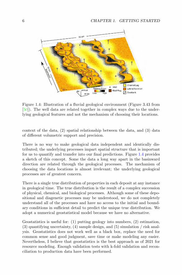
Figure 1.4: Illustration of a fluvial geological environment (Figure 3.43 from[50]). The well data are related together in complex ways due to the under-lying geological features and not the mechanism of choosing their locations.
context of the data, (2) spatial relationship between the data, and (3) dataof different volumetric support and precision.
There is no way to make geological data independent and identically dis-tributed; the underlying processes impart spatial structure that is importantfor us to quantify and transfer into our final predictions. Figure 1.4 providesa sketch of this concept. Some the data a long way apart in the basinwarddirection are related through the geological processes. The mechanism ofchoosing the data locations is almost irrelevant; the underlying geologicalprocesses are of greatest concern.
There is a single true distribution of properties in each deposit at any instancein geological time. The true distribution is the result of a complex successionof physical, chemical, and biological processes. Although some of these depo-sitional and diagenetic processes may be understood, we do not completelyunderstand all of the processes and have no access to the initial and bound-ary conditions in sufficient detail to predict the unique true distribution. Weadopt a numerical geostatistical model because we have no alternative.
Geostatistics is useful for: (1) putting geology into numbers, (2) estimation,(3) quantifying uncertainty, (4) sample design, and (5) simulation / risk anal-ysis. Geostatistics does not work well as a black box, replace the need forcommon sense and good judgment, save time or make modeling any easier.Nevertheless, I believe that geostatistics is the best approach as of 2021 forresource modeling. Enough validation tests with k-fold validation and recon-ciliation to production data have been performed.
1.1. INTRODUCTION 7
1.1.2 Notation and Some Mathematics
Upper case letters (X, Z, . . .) are often for random variables (RVs). Thesevariables are not entirely random, but they are not certain. Lower case let-ters (x, z, . . .) often represent for outcomes of random variables - perhapsmeasured data or perhaps simulated outcomes. Bold font (u, h,) is oftenreserved for vectors with some component in coordinate directions. The sym-bol ∈ means that something belongs to. The symbol ∀ means that somethingis true for all possibilities. The summation
∑and product
∏symbols are
commonly used.
The values of a regionalized variable over a domain A could be considered arandom function:
{Z(u),u ∈ A}We subscript a list of numbers with characters i, j, . . . or α, β, . . .. The lettern or N is often used to denote the number of data. The letter L is often usedto denote the number of realizations. The letter K is often used to denotethe number of rock types or the number of variables. Multiple realizations ofa multivariate block model could be denoted:
{zk,l(ui); i = 1, . . . , N ; k = 1, . . . ,K; l = 1, . . . , L}
Derivatives are essential for optimization. They are the slope of a functionwith respect to a variable. When the derivative is zero, the function is aminimum or maximum. They are rarely derived from first principals. Theycan be looked up in mathematical handbooks. The derivation of f(x) = x2
will be given in class and the generalization will be explained. The derivatiaveof f(x) = xn with respect to x is nxn−1 and we use this in geostatistics tominimize error variance. It is interesting to reflect on how efficient derivativesare for optimization considering the brute force alternative of exploring theentire space. In presence of 30 variables, conventional optimization wouldrequire computing the variable values that minimize 30 derivatives. If wewere to try that in a brute force manner by discretizing each variable by10 values, then we would have to evaluate the function1030 times, which isinconceivable.
Integration is used to solve the area or the average problem. The integrationof f(x) = x will be given in class and the generalization will be explained.The integration of f(x) = xn between the bounds of a and b by infinitesmalintervals dx is given by: ∫ b
a
xndx =1
n+ 1xn+1
∣∣∣ba
In general, the solution to the integration of different functions is found inthe literature. It is good if the geostatistician understand integration as it
8 CHAPTER 1. GETTING STARTED
relates to expected values (coming up). The fundamental theorem of calculuslays out the link between derivatives and integration.
In geostatistics, we often deal with linear sums such as Y = a1z1 + a2z2 +. . . + anzn =
∑ni=1 aizi. The quadratic form of a sum is a double sum:∑n
i=1
∑nj=1 aizi ajzj . The differentiation of a sum by a particular coefficient
is important in our build up to kriging.
∂(∑n
i=1
∑nj=1 aizi ajzj
)∂ai
= 2zi
n∑j=1
ajzj
This is part of the first exercise. These basic mathematical concepts arenot used on a day-to-day basis by a geostatistician or resource estimator;however, they form the basis of the algorithms we use and will help the restof the course make sense.
Matrix notation conveniently organizes numbers into rows and columns. Ma-trices of the same size could be added or subtracted. Matrix multiplicationis based on rows multiplied by columns: (mxn)(nxr) = mxr matrix. Theorder matters in matrix multiplication. The transpose of a matrix switchesthe rows and columns. Aside from simplicity of notation, we will only usematrices in the Citation to summarize dual kriging. Some additional linearalgebra will be required for that, but the essence of the idea should be clearwithout extensive background.
1.1.3 Stationarity
All statistical analysis requires a decision of how to pool the data for statisticalanalysis. The data and the study area are divided into reasonable subsets.It is unlikely that we would consider all of the data and the entire studyarea as one domain. The basis to subset the study area / data is necessarilysubjective and not a hypothesis because there is no reference to test against.We must:
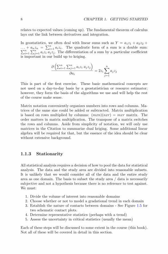
1. Divide the volume of interest into reasonable domains2. Choose whether or not to model a gradational trend in each domain3. Establish the nature of contacts between domains - See Figure 1.5 for
two schematic contact plots.4. Determine representative statistics (perhaps with a trend)5. Assess the uncertainty in critical statistics (usually the mean)
Each of these steps will be discussed to some extent in the course (this book).Not all of these will be covered in detail in this section.

1.1. INTRODUCTION 9
Figure 1.5: Illustration of a soft and hard boundary between two rock types.The distance axes is the distance into 2 from 1 (to the right) and into 1 from2 (to the left). The variable is on the ordinate axis.
The first aspect of stationarity is our decision of how to group the data for(geo)statistical analysis considering: (1) depositional zones of different qual-ity/spatial behaviour, (2) rock types within the zones, (3) spatially coherent.There is often a compromise geological precision and stable statistics. Thegeological meaning of the subsets is important. Sometimes called geologicalunits, rock types or domains. The precise terminology is context dependent.
The second aspect of stationarity is our decision of how the statistical param-eters vary in space. When a parameter can be assumed reasonably constantover the domain, then we refer to it as stationary. When we consider theparameter to be locally varying, then we refer to it as non-stationary. Somesketches will be drawn for the mean and variance in a 1-D setting.
A more formal definition of stationarity is sometimes preferred. The mostformal definition comes from time series and is paraphrased as a Stationaryprocess is one where the unconditional joint probability distribution does notchange when shifted in time. This connotes a location independence of statis-tical parameters and not the initial part of stationarity, that is, the choice ofa volume and the data within the volume to work with. Some specific formsof stationarity that are encountered include:
• Strict/strong stationarity - the entire probability distribution or spatiallaw of the variable is invariant under translation.• Weak stationarity - 1st and 2nd moments (mean, variance, covariance,. . .) are invariant under translation. First and second order stationarityare commonly assumed.• Intrinsic stationarity - increments of the regionalized variable separated
by specific lag (h) vectors are stationary. The variable could have a firstorder trend, but the increments are stationary. Higher order incrementscould be considered for more complex trends.• Quasi stationarity - the regionalized variable is assumed to follow con-
stant statistical parameters within spatial windows or, commonly, searchneighbourhoods.
10 CHAPTER 1. GETTING STARTED
• Trend stationarity - the regionalized variable is stationary (strong orweak) after removal of a trend. This is commonly assumed.
Increasingly in modern geostatistics we are explicitly defining or describingstationarity with auxilliary variable(s) like trend models and locally varyinganisotropy direction/magnitude models.
This course is not principally concerned with data collection, sampling the-ory, database integrity, but these issues must be mentioned. Standard bestpractices should be followed in all aspects of data collection, preparation andassaying. In general, geostatistical tools have no ability to detect problemdata: (1) errors appear like short scale geological microstructure, (2) biasescan be detected between data sources, but the truth cannot be discerned fromgeostatistical analysis. Special geostatistical analysis is required for noniso-topic data or data that is not sampled at the same locations.
The term compositing refers to the procedure of combining adjacent valuesinto longer down-hole intervals. The grade of each new interval is calculatedon the basis of the weighted average of the original sample grades. Theseare weighted by length and possibly by specific gravity and core recovery.Compositing typically leads to an average representing the entire thicknessof the zone or some regular length interval. There are special considerationsfor partial lengths at the end of drill holes and for partial lengths at theboundaries between domains.
The main reasons to composite are to (1) focus on a the scale of relevancefor mining resource estimation, (2) filter high frequency variations to show amuch better variogram, (3) mitigate the string effect in kriging to improveestimation [14], and (4) to be compliant with virtually all software that as-sumes the data represent the same volume. Length weighting is not a goodidea in estimation - it would only be correct if the variogram is a pure nuggeteffect. Regular length or bench composites are common. The length shouldbe small enough to permit resolution of the final simulated grid spacing.
Outliers and extreme values are a concern in deposits with highly skeweddistributions [46]. Clearly, errors in the data should be corrected and samplesthat are clearly erroneous should be rejected. We cannot blindly follow theadvice in statistics books since extreme values are justifiably removed in manycases for robust statistics, but these extreme values represent a significantfraction of the metal in many deposits. We cannot blindly use all data. Thegoal is to ensure: (1) no conditional (local) bias in the volumes around theoutliers, and (2) no unwarranted dependence on few samples. An outliershould be considered in a spatial context - a high value among other highvalues is of lesser concern. Cross validation could help with this. Tryingto isolate the high values into their own stationary domain mitigates theproblem.

1.1. INTRODUCTION 11
An advice given in the class is to follow local customs. This is not an excuseto be lazy, but a practical recommendation to make the resource estimateconsistent with past and similar resource estimates. We also consider prob-ability plots; looking for inflection points. Another helpful measure is theTukey fence i[58] where the upper threshold is considered:
zlimit = z0.75 + k (z0.75 − z0.25)
where k is 1.5 or 3.0 depending on the degree of outlier being considered andz0.75/z0.25 are quarties of the distribution (discussed below). Metal at risk,that is, the fraction of the metal based on a small number of extreme valuescould be considered.
The simulation approach in the Lesson [10] is neat, but a significant amountof work. This would be considered in advanced projects or when significantgeostatistical expertise is available.
1.1.4 Exercise W1-1
The objective of this exercise is to review some mathematical principles andto become familiar with some notation. Please write out by hand and show allimportant steps. Photograph/scan the pages and submit a PDF for marking.
1. Consider the following function f(x, y) = (ax + by)(x + y). Calcu-late the derivative of this function with respect to x, that is, calculate∂f(x, y)/∂x. Also calculate the derivative of the function with respectto y, that is: ∂f(x, y)/∂y.
2. Calculate the following integral:∫ 5
0
(1
2x2 + x3 − 1
4x5)dx
3. Consider the three matrices below:
A =
[5 22 3
]B =
[14
]C =
[2 3
]what is the result of AB and CB?
4. For the summation below, calculate the derivative ∂f(λi, i = 1, . . . , 4)/∂λkwith respect to λk where k is an index between 1 and 4. You may wantto compute all four and see if they are any different.
f(λi, i = 1, . . . , 4) =n∑i=1
n∑j=1
λiλj
12 CHAPTER 1. GETTING STARTED
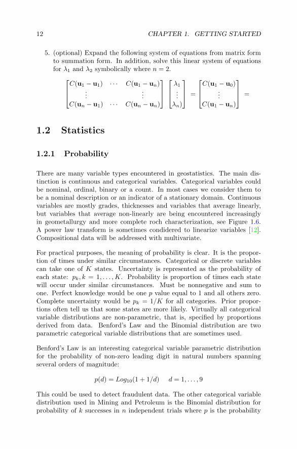
5. (optional) Expand the following system of equations from matrix formto summation form. In addition, solve this linear system of equationsfor λ1 and λ2 symbolically where n = 2.C(u1 − u1) · · · C(u1 − un)
......
C(un − u1) · · · C(un − un)
λ1...λn)
=
C(u1 − u0)...
C(u1 − un)
=
1.2 Statistics
1.2.1 Probability
There are many variable types encountered in geostatistics. The main dis-tinction is continuous and categorical variables. Categorical variables couldbe nominal, ordinal, binary or a count. In most cases we consider them tobe a nominal description or an indicator of a stationary domain. Continuousvariables are mostly grades, thicknesses and variables that average linearly,but variables that average non-linearly are being encountered increasinglyin geometallurgy and more complete roch characterization, see Figure 1.6.A power law transform is sometimes condidered to linearize variables [12].Compositional data will be addressed with multivariate.
For practical purposes, the meaning of probability is clear. It is the propor-tion of times under similar circumstances. Categorical or discrete variablescan take one of K states. Uncertainty is represented as the probability ofeach state: pk, k = 1, . . . ,K. Probability is proportion of times each statewill occur under similar circumstances. Must be nonnegative and sum toone. Perfect knowledge would be one p value equal to 1 and all others zero.Complete uncertainty would be pk = 1/K for all categories. Prior propor-tions often tell us that some states are more likely. Virtually all categoricalvariable distributions are non-parametric, that is, specified by proportionsderived from data. Benford’s Law and the Binomial distribution are twoparametric categorical variable distributions that are sometimes used.
Benford’s Law is an interesting categorical variable parametric distributionfor the probability of non-zero leading digit in natural numbers spanningseveral orders of magnitude:
p(d) = Log10(1 + 1/d) d = 1, . . . , 9
This could be used to detect fraudulent data. The other categorical variabledistribution used in Mining and Petroleum is the Binomial distribution forprobability of k successes in n independent trials where p is the probability

1.2. STATISTICS 13
Figure 1.6: Illustration of the nature of averaging of different continuousvariables.
of one trial:
f(k, n, p) =n!
k!(n− k)!pk(1− p)n−k
As mentioned, these are uncommon. Non-parametric and, often, non-stationarydistributions are used for categorical variable distributions.
The universal approach to represent uncertainty in a continuous variable isthe cumulative distribution function (CDF). Replace unknown truth ztrue bya random variable Z. Cumulative distribution function (CDF) of an RV isdefined as:
F (z) = Prob {Z ≤ z}The CDF F (z) is non decreasing within [0, 1]. F (zmin) = 0 and F (zmax) = 1.The CDF is flexible in representing great uncertainty (F (z) spread over a largerange of z) and certainty (F (z) a step function at the certain z value).
There are three ways to infer a CDF:
1. Degree of belief - for global parameters that are inaccessible2. Proportions from data - global probabilities and distributions3. Mathematical model - local conditional parameters
The probability of Z occurring in an interval from a to b (where b > a) is

14 CHAPTER 1. GETTING STARTED
Figure 1.7: Illustration of the generating mechanism underlying the Gaussiandistribution - the sum of independent and identically distributed randomvariables.
the difference in the cdf values evaluated at points b and a. The probabilitydensity function (pdf) is the derivative of the cdf, if it exists:
f(z) = F ′(z) = limdz→0
F (z + dz)− F (z)
dz≥ 0
The CDF and PDF contain equivalent information. It may be convenient toconsider one in mathematical calculations / computer implementations andanother in visualization or for other calculations.
A parametric distribution is one where F (z) or f(z) is given by an equationwith some parameters. There may or may not be a generating mechanism forthe probabilities. Most earth science distributions are non-parametric andinferred by proportions from data.
The generating mechanism for the Gaussian distribution is summarized incentral limit theorem (sum of many iid→ Gaussian), as shown on Figure 1.7.
y = G−1(F (z)) or Y =Z −mσ
g(y) =1√2πe−y2
2
The multivariate Gaussian distribution is used extensively in geostatisticsbecause it is simply parameterized and tractible.
The lognormal distribution is closely related to the Gaussian or normal distri-bution and is also common in geostatistics. Z logN(m,σ) when Y = ln(z)is N(α, β2). The parameters are related by:
α = ln(m)− β2/2 β2 = ln
(1 +
σ2
m2
)
1.2. STATISTICS 15
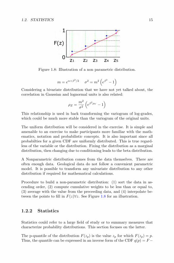
Figure 1.8: Illustration of a non parametric distribution.
m = eα+β2/2 σ2 = m2
(eβ
2
− 1)
Considering a bivariate distribution that we have not yet talked about, thecorrelation in Gaussian and lognormal units is also related:
ρZ =m2
σ2
(eβ
2ρY − 1)
This relationship is used in back transforming the variogram of log-grades,which could be much more stable than the variogram of the original units.
The uniform distribution will be considered in the exercise. It is simple andamenable to an exercise to make participants more familiar with the math-ematics, notation and probabilistic concepts. It is also important since allprobabilties for a given CDF are uniformly distributed. This is true regard-less of the variable or the distribution. Fixing the distribution as a marginaldistribution, then changing due to conditioning leads to the beta distribution.
A Nonparametric distribution comes from the data themselves. There areoften enough data. Geological data do not follow a convenient parametricmodel. It is possible to transform any univariate distribution to any otherdistribution if required for mathematical calculations.
Procedure to build a non-parametric distribution: (1) sort the data in as-cending order, (2) compute cumulative weights to be less than or equal to,(3) average with the value from the preceeding data, and (4) interpolate be-tween the points to fill in F (z)∀z. See Figure 1.8 for an illustration.
1.2.2 Statistics
Statistics could refer to a large field of study or to summary measures thatcharacterize probability distributions. This section focuses on the latter.
The p-quantile of the distribution F (zp) is the value zp for which F (zp) = p.Thus, the quantile can be expressed in an inverse form of the CDF q(p) = F−
16 CHAPTER 1. GETTING STARTED
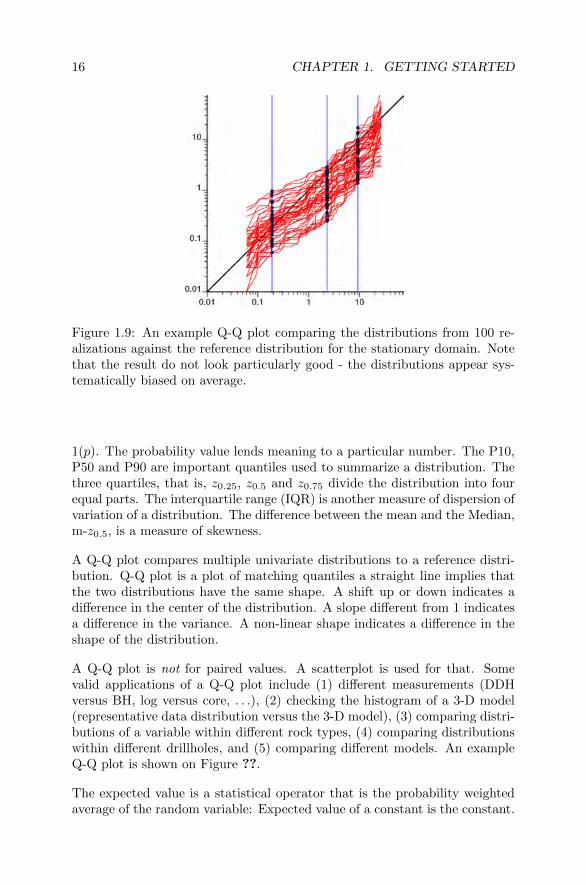
Figure 1.9: An example Q-Q plot comparing the distributions from 100 re-alizations against the reference distribution for the stationary domain. Notethat the result do not look particularly good - the distributions appear sys-tematically biased on average.
1(p). The probability value lends meaning to a particular number. The P10,P50 and P90 are important quantiles used to summarize a distribution. Thethree quartiles, that is, z0.25, z0.5 and z0.75 divide the distribution into fourequal parts. The interquartile range (IQR) is another measure of dispersion ofvariation of a distribution. The difference between the mean and the Median,m-z0.5, is a measure of skewness.
A Q-Q plot compares multiple univariate distributions to a reference distri-bution. Q-Q plot is a plot of matching quantiles a straight line implies thatthe two distributions have the same shape. A shift up or down indicates adifference in the center of the distribution. A slope different from 1 indicatesa difference in the variance. A non-linear shape indicates a difference in theshape of the distribution.
A Q-Q plot is not for paired values. A scatterplot is used for that. Somevalid applications of a Q-Q plot include (1) different measurements (DDHversus BH, log versus core, . . .), (2) checking the histogram of a 3-D model(representative data distribution versus the 3-D model), (3) comparing distri-butions of a variable within different rock types, (4) comparing distributionswithin different drillholes, and (5) comparing different models. An exampleQ-Q plot is shown on Figure ??.
The expected value is a statistical operator that is the probability weightedaverage of the random variable: Expected value of a constant is the constant.
1.2. STATISTICS 17
The expected value is a probability weighted average:
E{·} =
∫ zmax
zmin
·f(z)dz
The most important expected value is the mean:
m = E{Z} =
∫ zmax
zmin
zf(z)dz
In theory, the expected value is an integral (probability weighted average) Inpractice, the expected value is estimated by a weighted average:
m =n∑i=1
wizi
The mean is also known as the first moment, that is, the center of mass of theprobability density function. The variance is a second order moment definedas:
σ2 = E{[Z −m]2} = E{Z2} −m2
The variance is a measure of the spread of the data from the mean. Thestandard deviation is the square root of the variance. It also measures datavariability from the mean. The dimensionless coefficient of variance (CV)is the ratio of the standard deviation over the mean (σ/m). This worksfor positive variables. Conventional wisdom indicates that a variable with aCV < 0.4 is not that variable and potentially straightforward to model. Avariable with CV > 2.0 is quite variable and the domain should be consideredfor subdivision. These are not fixed values, but general guidelines.
The mean is the correct number to replace a probability distribution whenthe variable under consideration averages linearly. Consider mass percentagemeasurements of 9, 1, 1 and 1 for four units of rock of equal mass. If the pileswere combined, the mass percentage would be 3 and not a quantile or morerobust estimator. This is true for mass fractions, volume fractions, rock typeproportions and other variables that average linearly. The correct effectivevalue is not the median, mode, Exceptions are when the variable does notaverage linearly such as color, rate constants (permeability, work index, etc.).
Many geostatistical calculations require continuous variables to exactly followthe standard normal distribution, that is, N(0, 1) normal with a mean of zeroand a variance of one. The normal score transform is used to transform non-normal data following any distribution to a Gaussian or normal distribution.The steps: (1) determine the representative Z-variable distribution FZ(z), (2)transform each z data by matching quantiles, y = G−1(FZ(z)) where G(y) isthe CDF of the N(0, 1) distribution. Figure 1.10 shows this for one z valueof 10.0. This is taken from the Lesson [51] on the normal score transform.

18 CHAPTER 1. GETTING STARTED
Figure 1.10: Illustration of the normal score transform. A value of 10 istransformed.
Regarding the normal score transform, a representative distribution FZ(z) isthe most important consideration. Spikes of constant values coming from de-tection limit or round off are also a concern. The ties must be broken to avoida spike in Gaussian units that is not allowed. Entirely random despiking leadsto a too-high nugget effect in the final variogram. A combination of a localaverage and random despiking has been shown to work well. Another op-tion is to isolate the barren/unmineralized material into its own domain/rocktype.
1.2.3 Declustering
The data are considered trustworthy (although every measurement is associ-ated with some error), but they are almost certainly collected in a preferentialmanner. Correcting the statistics for this will be done with declustering anddebiasing. Although clear when the mathematics are reviewed, it is impor-tant to note that declustering does not change the data values. The dataremain unchanged. The weight applied to the data may vary. The represen-tative distribution for transformation and other calculations may come fromanother source, but the data do not change.
Data are rarely collected to be statistically representative: Interesting (best)

1.2. STATISTICS 19
area delineated more completely, Samples taken preferentially from good qual-ity rock. These data collection practices should not be changed; they lead tothe best economics and the greatest number of data in portions of the studyarea that are the most important. There is a need, however, to adjust thehistograms and summary statistics to be representative of the entire volumeof interest
Declustering techniques assign each datum a weight based on closeness tosurrounding data: wi, i = 1, . . . , n histogram and cumulative histogram usewi, i = 1, . . . , n instead of 1/n. Debiasing uses a secondary variable or trendto establish representative histogram or proportions
Historical mapping algorithms correct for preferential sampling: no need fordeclustering in inverse distance or OK. There is a need for representativeproportions and histograms in modern geostatistics: Checking models, Globalresource assessment, and as an input to simulation. Simulation does notcorrect for preferential sampling even though kriging is used inside simulation.Cokriging with a secondary data does not correct the distribution: correlationwith the rank order of the data is used the conditional distributions are notused directly
Declustering weights are taken proportional to the areas or volumes of inter-est. Weights are very sensitive to the border. Despite the apparent criticismof nearest neighbor declustering, the technique is being used increasingly andperhaps even more than the competing techniques discussed below.
Cell Declustering is considered to be more robust in 3-D and when the limitsare poorly defined, see Lesson [18] and Figure 1.11:
1. divide the volume of interest into a grid of cells l = 1, . . . , L2. count the occupied cells Lo and the number in each cell nl, l = 1, . . . , Lo3. weight inversely by number in cell (standardize by Lo)
Fixing the cell size and changing the origin often leads to different declusteringweights. To avoid this artifact a number of different origin locations areconsidered for the same cell size and the weights are averaged for each originoffset, see Figure 1.12. It is highly unlikely, but if a data falls on a cellboundary it is randomly moved to a possible cell.
The cell size should be the spacing of the data in the sparsely sampled areas.The declustered mean is often plotted versus the cell size for a range of cellsizes a diagnostic plot that may help get the cell size. The long range fea-tures of the diagnostic plot are often influenced by trends and non-stationaryfeatures.
Declustering by Conventional Estimation. Perform an estimation of grid

20 CHAPTER 1. GETTING STARTED
Figure 1.11: Illustration of the concept of cell declustering. A grid of cells isplaced over the data, the number of data within each cell counted and theweight is inversely proportional to the number of data in the cell.
Figure 1.12: Illustration of how the origin of the cell declustering grid networkis moved to stabilize the results.

1.2. STATISTICS 21
block values within the applicable RT limits and within reasonable distanceto the data. Consider inverse distance or kriging. Accumulate the weightgiven to each data in the estimation procedure. Clustered data will receiveless weight overall. Sensitive to the search, variogram, May not work well ifthe string effect of kriging is a problem. Results are perfectly consistent withkriging a nice property
What do we do when there are too few data or the data are not representative?Nothing, unless there is some secondary information. An empirical calibra-tion approach is sometimes referred to as debiasing or soft data declustering:(1) map a secondary variable X at all locations that could be geophysical,structural or some kind of trend model, (2) develop a bivariate relationshipbetween X and the Y variables, and (3) generate a distribution of Y bycombining conditional distributions. The secondary variable is somethinggeometric, geophysical or geological.
There is no recipe for correct application. Our goal is to go beyond a limitedsample to the underlying true population. It is essential to decluster faciesproportions as well as the distributions of continuous variables. Future geo-statistical analysis will depend heavily on simple statistics inferred early inthe modeling efforts.
The volume of influence method is gaining ascendancy - fewer artifacts thanthought. The sensitivity to the border actually helps infer a representativedistribution. Trend models somewhat alleviate the need for declustering, buta good trend model will be built considering declustering weights.
1.2.4 Exercise W1-2
The objective of this exercise is to review some probabilistic concepts andto continue becoming familiar with notation. Please write out by hand andshow all important steps. Photograph/scan the pages and submit a PDF formarking.
Consider the uniform distribution specified below:
1. Write the definition and equation for the cumulative distribution func-
22 CHAPTER 1. GETTING STARTED
tion (cdf) of the uniform distribution.2. What is the value of c that makes f(z) a licit probability distribution?
Write your answer in terms of a and b.3. What is the expected value (or mean) of the variable Z in terms of a,b, and c? Work out the integral.
4. What is the variance of the variable Z in terms a, b, and c? Work out theexpected value of Z2 and solve for the variance using σ2 = EZ2−[EZ]2.
5. What is the width of the 90% probability interval expressed in terms ofa and b? Use the results of Question 1 and solve for the 5th and 95thpercentiles.
1.3 More Prerequisites
1.3.1 Bayes’ Law
The arithmetic of probability intrigued Thomas Bayes. He thought deeply onthe subject and formulated the fundamental principles that are still used to-day. It was clear to Bayes that probability is the proportion of times somethingwould happen in similar circumstances, probability could not be negative andthe sum of probabilities would be one in a closed set. The definition of aconditional probability and Bayes Law are fundamental to probability andstatistics:
P (A|B) =P (A and B)
P (B)P (B|A) =
P (A and B)
P (A)
P (A|B) = P (A) · 1
P (B)· P (B|A)
Conditional probability is the prior probability modified by the evidence. Therarity of the evidence and the relevance of the evidence (likelihood) enter theequation. Additional details and an example to geostatistical mapping arecontained in a Lesson [21].
The example on Figure 1.13 is developed in the class. The definition ofconditional probability is used extensively in geostatistics. The meaning ofthis is revealed in the requirement to standardize probabilities once evidenceis available.
1.3.2 Coordinate Rotation and Anisotropy
Coordinates and anisotropy are important topics in geostatistics. The funda-mentals of this will also set the stage for principal component analysis (PCA)

1.3. MORE PREREQUISITES 23
Figure 1.13: Illustration of the definition of conditional probability.
coming later in the week.
The spatial coordinates of a deposit form a metric space with a measure ofdistance d where: d(x, y) ≥ 0, d(x, y) = 0 ⇐⇒ x = y, and d(x, y)+d(y, z) ≥d(x, z). Measures of distance include:
• Chebyshev Distance - maximum along any coordinate• Manhattan Distance - measured along axes at right angles• Euclidean Distance - ordinary straight line
h =
√(hmajamaj
)2
+
(hminamin
)2
+
(hterater
)2
• Minkowski Distance - p exponent (pM = 1, pE = 2)
Shortest path distances, LVA, Dijkstra algorithm . . .
Real world coordinates are often UTM Easting (X), UTM Northing (Y) andmeters above sea level (Z). These coordinates lead to a natural left hand rule.Imagine your left hand with the thumb sticking upward (Z), the middle fingerpointing to your right (X) and your pointing figure pointing away from you(Y). This is the starting point for coordinate rotation.
New coordinate systems should never be invented on the fly. Modern softwareallows for rotated grid models without changing the actual coordinates.
Aeronautics definition of anisotropy with roll, pitch and yaw is very intuitive,

24 CHAPTER 1. GETTING STARTED
Figure 1.14: Illustration for the rotation around one axis
but not used in geology.
Coordinate rotation: left hand rule. The Lesson [26] is helpful. Consider asuccession of three 2-D rotations (see Figure 1.14 for elementary rotation:
1. Clockwise positive around vertical (angle one)2. Down negative around what was X (angle two)3. Polite positive around what was Y (angle three)
Every software is different. Three angles of rotation specify the major, minorand tertiary directions. The standardized Euclidean distance enters virtuallyall calculations.
1.3.3 Grids for Geologicical Modeling
Cartesian coordinates and regular 3-D grids are fairly straightforward to un-derstand. Stratigraphic-like grids for tabular deposits are important to cap-ture undulations and thickness variations. Generalized tetrahydra grids willbecome more popular as software libraries are established.
Considering a regular Cartesian grid, an important consideration is the gridsize. There are many considerations for this including (1) the supporting datafor predictions - one quarter the data spacing is a reasonable natural grid size

1.3. MORE PREREQUISITES 25
Figure 1.15: Two illustrations of typical tabular deposits that would be con-sidered within the framework of simple tabuluar deposits.
recommendation (smaller grid sizes will not be estimated more reliably andlarger grid sizes would lose information), (2) the desire to respect geologicalboundaries - smaller blocks or subblocks are desired to capture surfaces thatwould not be represented by coarse blocks, and (3) engineering considerationswhere the block size is influenced by pit or stope design considerations. A highresolution grid is recommended even if the block estimates are no better thana lower resolution grid - at least the result will respect geological boundariesand support engineering calculations.
Tabular Deposits
Simple tabular deposits are commonly encountered. There are stratigraphicdeposits, lateritic weathered deposits, simple veins, shear zones and manyother situations where a tabular geometry is encountered. A first considera-tion in the case of tabular deposits is to establish a reference plane. The topor hangingwall and bottom or footwall are established relative to the refer-ence plane. Figure 1.15 shows two example reference surfaces; one flat andone steeply dipping.
Given arbitrarily oriented data that intersect a tabular structure, we couldconsider total least squares plane fitting π : ax+ by+ cz = d to determine thereference plane. The Eigenvector corresponding to the minimum Eigenvalueof ATA defined the normal vector:
A =
x1 − x y1 − y z1 − zx2 − x y2 − y z2 − z
......
...xn − x yn − y zn − z
This is like PCA (defined below) where the major axes of continuity are

26 CHAPTER 1. GETTING STARTED
calculated through a cloud of points. The A matrix could be considereda covariance matrix (defined below). In any case, by default (horizontal orvertical), manual specification or automatic calculation a reference plane mustbe defined to model tabular deposits.
The commonly accepted approach is to model one position and multiple thick-ness values relative to the reference plane. Modelling multiple positions wouldoften lead to crossing surfaces or unreasonably large thicknesses. The mostcontinuous surface would be chosen for the position variable, then thicknessesrelative to that would be modeled.
Figure 1.16 illustrates the overall approach. Eight drill holes are shown atthe top where three do not intersect the structure - tje drillholes with dashedlines are the ones that do not intersect the structure (Figure 1.16.a). Thered line is the reference plane and the black dots represent the top and baseof the structure of interest. Figure 1.16.b illustrates the modeling of thetop structure (chosen as the position variable) by the blue line. There maybe multiple realizations for the top structure. The drill holes that do notintersect the structure are not considered in modeling of the top position. Inan inverted manner Figure 1.16.c shows the thickness modeled as the greensurface below the blue datum of the reference position. Once again, thedrill holes that do not intersect the structure are ignored. Figure 1.16.dshows the modeled position and thickness put back together relative to thereference plane. Finally, Figure 1.16.e shows that the extent of the positionand thickness are clipped to account for holes and for limits within the planeof continuity.
Missing values should be ignored, then clipped by boundary modeling. Theexact nature of the pinch out or termination may not be exactly reproduced,but this is of little consequence in general given the thin and laterally extensivenature of these deposits.
Modeling continuous properties within tabular deposits defined by a top andbottom (perhaps multiple realizations of the top and bottom are available)required the use of stratigraphic coordinates. Figure 1.17 shows four commoncases for stratigraphic coordinates: proportional, erosion - base conforming,onlap - top conforming, and offlap - arbitrary surface conforming.
The coordinate perpendicular to the reference plane (Z in the equation below)is modified so that a flattened or relative coordinate is considered.
zrel(x, y) =z(x, y)− zbase(x, y)
ztop(x, y)− zbase(x, y)· T
Where x and y represent coordinates definint the reference plane of continuity.If the transform is proportional, then the top and bottom are taken locally.If the transform is erosion, then the top is replaced by the bottom translated

1.3. MORE PREREQUISITES 27
Figure 1.16: Illustration of how we model the position, then thickness, thenassemble everything in original units.

28 CHAPTER 1. GETTING STARTED
Figure 1.17: Four common cases for stratigraphic coordinates.
upward by a constant. If the transform is onlap, then the bottom is replacedby the top translated downward by a constant. The top and base are definedarbitrarily in the case of offlap. This transformation can be reversed at anytime.
The 3-D models of tabular deposits should not be shown in flattned space.Highly deviated drill holes relative to the plane of continuity are particularlyproblematic; some form of geometric data imputation must be considered.
1.3.4 Exercise W1-3
The objective of this exercise is to become familiar with the use of declusteringto infer a representative probability distribution. The declustering softwarein GSLIB or any other software could be used.
1. Consider the Au variable in the skarn2d.dat data file. Decluster the dataset using cell declustering. Cell declustering is widely used because itis robust and not very sensitive to edge effects.Plot a location map of the sampling locations and propose a reasonablecell declustering cell size based on the data spacing in sparsely sampledareas. Also plot a naive (no declustering) histogram of the variable ofinterest.Run cell declustering for a range of cell sizes: explain your choice ofparameters in your assignment. Plot the declustered mean versus cellsize, then on the basis of this plot and data spacing, choose a cell size,and justify your choice.Plot a histogram of the variable using the declustering weights andcomment on differences with the unweighted histogram.
2. One method to construct a trend model for potential soft data decluster-ing (debiasing) and global mean inference is global kriging. Use globalkriging with a long range and large nugget effect for creating a trendmodel. Visualize the trend model and calculate a histogram of the trend

1.4. BIVARIATE STATISTICS 29
Figure 1.18: Schematic illustration of the high dimension of geostatisticalproblems: K variables at N locations.
model for the global mean. Compare with the previous question.3. Consider the Au variable in the Misima.dat data file. Have a quick look
at the data and run declustering following the principles of Question 1.
1.4 Bivariate Statistics
1.4.1 Bivariate Distributions
Geostatistical modeling considered a very high dimensional distribution ofvariables and locations. This high dimensional distribution is almost alwaysunderstood through models of the bivariate distributions. Figure 1.18 illus-trates the magnitude of the distributions we are dealing with.
The bivariate CDF tells us everything about how two variables are related:
FX,Y (x, y) = Prob{X ≤ x;Y ≤ y}
This is a contour map in the space of the two variables X and Y . The

30 CHAPTER 1. GETTING STARTED
Figure 1.19: Bivariate distribution with marginal and conditional.
bivariate PDF contains equivalent information:
fX,Y (x, y) =∂2FX,Y (x, y)
∂x∂y
Like the univariate case, the PDF integrates to the CDF. It may be conve-nient to consider one or the other for visualization or mathematical purposes.Figure 1.19 shows a bivariate with marginal, joint and conditional distribu-tions.
In many cases of presenting bivariate distributions it matter which variableis shown on the X abscissa axis and which is shown on the Y ordinate axis.If one of the variables could be considered an independent or data variable,then it is shown on the X. By convention, the dependent variable is shownon the Y axis. The only conditional distribution that matters is the one ofY |X = x. Connecting the expected values of the conditional distributions ofY |X = x would generate a conditional expectation or regression curve. Givenknowledge of X = x, then this curve would give the best estimate of Y .
The bivariate Gaussian probability distribution is sometimes used. There arefew parametric distributions. The Gaussian PDf is given by:
gXY (x, y) =1
2π√
1− ρ2exp
{− 1
2(1− ρ2)[x2 − 2ρxy + y2]
}
E{Y |X = x} = µY + ρσYσX
(x− µX)
V ar{Y |X = x} = σ2Y (1− ρ2)
Some properties of this distribution are seen again in the multivariate distri-bution: (1) conditional expectations are linar functions of conditioning data,and (2) conditional variances are data-value independent.

1.4. BIVARIATE STATISTICS 31
Figure 1.20: Illustration of how a direct relationship leads to a positive co-variance and an inverse relationship makes the covariance negative.
1.4.2 Covariance and Correlation
Univariate distributions are often summarized by their first two moments:the mean and variance. A bivariate distribution is summarized by the covari-ance or the standarided correlation coefficient. The covariance is a two-pointmeasure used throughout statistics and geostatistics. The covariance betweenrandom variables X and Y is written:
Cov{X,Y } = CXY = E{[X −mX ][Y −mY ]}= E{XY } −mXmY
The expected value is a double integral over X and Y . In practice it iscalculated as a sum over available pairs. The covariance is a measure ofthe closeness to a perfect linear relationship. If the linear relationship is adirect one, then the covariance will be positive and if the relationship is aninverse one, then the covaraince will be negative. Figure 1.20 illustrates thisscematically.
The covariance has the units of X multiplied by Y . It is common to con-sider the correlation coefficient, that is, the standardized covariance that fallswithin -1 and +1:
correlation ρ = CXY /(σX · σY ) ∈ [−1,+1]
If the bivariate data were bivariate Gaussian, then the covariance or corre-lation with the variances would completely define the distribution. In manypractical cases, there are complex features in the data that make the covari-ance an incomplete measure.

32 CHAPTER 1. GETTING STARTED
1. Outliers can enhance an otherwise poor correlation or reduce an other-wise good correlation
2. Non-linear relationships would be captured to some extent by the cor-relation coefficient, but the conditional distributions would have lessvariance than implied.
3. Constraints from mineralogy or fractional measurements (total copperand acid soluble copper, for example) are not fully captured by thecorrelation coefficient.
4. The proportional effect or heteroscedasticity are not captured by thecorrelation coefficient.
The correlation coefficient described above is sometimes called the Pearsoncorrelation coefficient - named after Karl Pearson a famous statistician. Thecorrelation coefficient is sensitive to extreme values (outliers) and an alterna-tive was proposed by Charles Spearman. The Spearman correlation coefficientis also known as the rank correlation coefficient. The idea is to rank trans-form the both variables from 1 to n - preserving the order, then compute thePearson correlation coefficient on the rank order values and not the originaldata values. The Spearman correlation coefficient could be used to establishwhether extreme values are destabilizing the correlation.
The correlation coefficient is not the coefficient of determination R2 althoughit would be R if the distribution were bivariate Gaussian. it is better toreserve the use of R2 for a measure of goodness in prediction. This will becovered later.
Uncorrelated does not equal independence - there could be some dependencecaused by one or more of the considerations mentioned above.
Correlation does not imply causation. This is a mainstay of modern statistics.There are many examples including the correlation between crime rate andnumber of places of worship per square kilometer. They may be related, butthrough something else such as population density. Using variables withoutcause and effect is still possible for prediction if the results are stable; justnot used for explanation.
1.4.3 Principal Component Analysis
Principal Component Analysis (PCA) is well established and very interestin-gin modern data science and geostatistics. It is nice to see something noveland interesting in the first week - aside from an overview and review of statis-tics.
PCA is a classic dimension reduction and decorrelation technique that was

1.4. BIVARIATE STATISTICS 33
developed by Pearson [47] and Hotelling [32] and adapted to geostatistics inthe 70s and 80s. PCA transforms multivariate data that are correlated in anarbitrary manner into orthogonal linear combinations of the original variables,that is, factors that are all uncorrelated. It is useful to imagine rotation inthe high dimension space of the data. The position of the data in the highdimensional space of the data does not change, but the new coordinates ofthe PCA make the data appear uncorrelated. The direction where the datashow the most variance is the first principal component and they are orderedin decreasing variance. The Lesson [4] by Ryan Barnett is a good place foran overview.
The reasons to consider PCA are threefold.
1. Understand underlying factors - there are times when understandingthe principal components - the independent directions that explain thevariability in the data, explains aspects of the nature of the multiplevariables. This is sometimes possible with data in geostatistics.
2. Reduce dimension - the principle components are ordered in decendingorder of the variance they explain. At a certain point, perhaps when99% of the variance has been explained, the remaining pricipal compo-nents can be dropped from the analysis.
3. Decorrelation - the principal components are uncorrelated with eachother and it is possible to simulate them independently, then the corre-lation structure is reintroduced in the reverse rotation.
Consider K variables that are standardized (centered and scaled to have avariance of one). This could be done by a simple standardization (subtract themean and divide by the standard deviation) or by a normal score transform.We would often consider an normal score transform since the shape of thedistribution and outliers are managed. The only reason to consider a simplestandardization is if kriging or some other linear technique is being consideredfor the PCA factors.
From an intuitive or graphical perspective, PCA amounts to rotate the Kdimensional coordinate system to make the variables uncorrelated. The valuesrepresented in the rotated space are referred to as principal components. Thisis done by the spectral decomposition of the KxK covariance matrix of thevariables. The principal components are uncorrelated, but do not have unitvariance. They are ordered so that the first has the greatest variability andthe last has the least. Details of this are given in the fourth week (lastChapter), but participants are asked to go through the steps here to gain anunderstanding of covariance and multivariate data.
The concept of PCA linked to coordinate rotation is powerful. Think aboutleaving the multivariate data at their locations and rotating the coordinatesso that the data appear uncorrelated (see Figure 1.14 for an illustration).
34 CHAPTER 1. GETTING STARTED
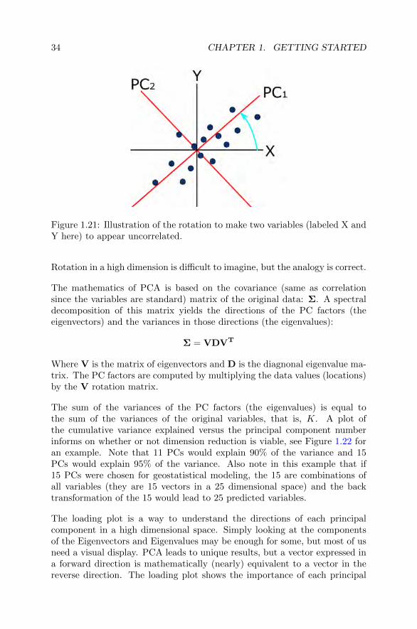
Figure 1.21: Illustration of the rotation to make two variables (labeled X andY here) to appear uncorrelated.
Rotation in a high dimension is difficult to imagine, but the analogy is correct.
The mathematics of PCA is based on the covariance (same as correlationsince the variables are standard) matrix of the original data: Σ. A spectraldecomposition of this matrix yields the directions of the PC factors (theeigenvectors) and the variances in those directions (the eigenvalues):
Σ = VDVT
Where V is the matrix of eigenvectors and D is the diagnonal eigenvalue ma-trix. The PC factors are computed by multiplying the data values (locations)by the V rotation matrix.
The sum of the variances of the PC factors (the eigenvalues) is equal tothe sum of the variances of the original variables, that is, K. A plot ofthe cumulative variance explained versus the principal component numberinforms on whether or not dimension reduction is viable, see Figure 1.22 foran example. Note that 11 PCs would explain 90% of the variance and 15PCs would explain 95% of the variance. Also note in this example that if15 PCs were chosen for geostatistical modeling, the 15 are combinations ofall variables (they are 15 vectors in a 25 dimensional space) and the backtransformation of the 15 would lead to 25 predicted variables.
The loading plot is a way to understand the directions of each principalcomponent in a high dimensional space. Simply looking at the componentsof the Eigenvectors and Eigenvalues may be enough for some, but most of usneed a visual display. PCA leads to unique results, but a vector expressed ina forward direction is mathematically (nearly) equivalent to a vector in thereverse direction. The loading plot shows the importance of each principal

1.4. BIVARIATE STATISTICS 35
Figure 1.22: Example plot of the cumulative variance explained versus thePC number for 25 variables.
component and the contribution of each variable to each principal component.
Regarding the exercise, a normal score transform of the principal componentsmay impart some residual non-zero correlation between the transformed vari-ables. This would not happen with multivariate Gaussian data, but real dataare rarely truly multivariate Gaussian.
1.4.4 Exercise W1-4
The objectives of this exercise are to learn how to normal score transformdata, calculate a correlation matrix and apply principal component analy-sis to determine orthogonal combinations of variables which account for alarge amount of variation. Consider the Ni, Fe, SiO2 and MgO variables innilat.dat.
1. Plot cross plots between all variables of interest.2. Normal score transform the data. Note that you do not need to use
declustering weights for this exercise, but you may optionally also com-plete this exercise with declustering weights to see if there are any dif-ferences in the correlations.
3. Calculate a correlation matrix for the normal score transformed data.Also plot the normal score bivariate distributions and comment on anychanges to the bivariate from Question 1.
4. Run principal component analysis on the normal score transformed vari-ables to construct orthogonal linear combinations of the normal scoredata.
5. See how the linear combinations are constructed and visualize the load-

36 CHAPTER 1. GETTING STARTED
ing of each variable on to the principal components to see which vari-ables explain the greatest amount of variance in the data set.
6. Normal score transform the principal components and repeat Question3. Compare the results and comment on any differences.
Chapter 2
Variograms and Kriging
This week presents much of classic Matheronian geostatistics. Variograms,volume variance relations (change of support) and kriging are topics that willretain importance despite advances in computing algorithms and machinery.
2.1 Variograms I
2.1.1 The Variogram
Two point statistics are used throughout geostatistics. The covariance andcorrelation coefficient were presented in the previous chapter.
Cov{X,Y } = CXY = E{[X −mX ][Y −mY ]}= E{XY } −mXmY
correlation ρ = CXY /(σX · σY )
The variogram is closely related to these measures. The variogram gainedpopularity in early geostatistics because it was considered a more robustalternative in presence of non-stationarity.
Central to the variogram is the concept of a vector lag distance h that is adistance in a particular direction. Experimental pair separated approximatelythe vector distance are assembled and the variogram is calculated as theexpected value of the squared difference in the values separated by the lag:
variogram 2γ(h) = E{[Z(u)− Z(u + h)]2}
37

38 CHAPTER 2. VARIOGRAMS AND KRIGING
Figure 2.1: Illustration that the variogram is the squared distance from the1:1 line.
Figure 2.2: Concept of why variogram persisted instead of covariance.
The variogram is calculated for a set of lag distances to obtain a continuousfunction. Figure 2.1 shows a geometric interpretation of the variogram - theexpected squared distance from the 1:1 line.
Under stationarity the variogram, covariance and correlation coefficient areequivalent tools for characterized two-point correlation:
2γ(h) = E{Z(u)2 − 2Z(u)Z(u + h) + Z(u + h)2}= E{Z(u)2} −m2 − 2
(E{Z(u)Z(u + h)} −m2
)+ E{Z(u + h)2} −m2
= σ2 − 2C(h) + σ2
= 2σ2 − 2C(h)
The stationarity of the variogram lag over the domain allows experimental
2.1. VARIOGRAMS I 39
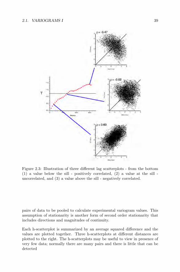
Figure 2.3: Illustration of three different lag scatterplots - from the bottom(1) a value below the sill - positively correlated, (2) a value at the sill -uncorrelated, and (3) a value above the sill - negatively correlated.
pairs of data to be pooled to calculate experimental variogram values. Thisassumption of stationarity is another form of second order stationarity thatincludes directions and magnitudes of continuity.
Each h-scatterplot is summarized by an average squared difference and thevalues are plotted together. Three h-scatterplots at different distances areplotted to the right. The h-scatterplots may be useful to view in presence ofvery few data; normally there are many pairs and there is little that can bedetected

40 CHAPTER 2. VARIOGRAMS AND KRIGING
2.1.2 Variogram Calculation
Variography involves (1) calculation, (2) interpretation, and (3) modeling.The three overlap, but it is reasonable to learn about the steps in this order.An important assumption of stationarity is embedded in the concept of thevariogram, that is, the spatial statistics depend on the lag separation vector,but are independent of location. The expected variability between two lo-cations separated by 120m in the North-South direction is the same for allpositions within the domain. This assumptions makes it possible to calcula-tion variograms from the available data. The lag vector with some toleranceis scanned over all pairs of data and the expected variability is calculateddirectly. The concept that the lag vectors float and are anchored is a keyconcept in variography.
Another key concept that arises from the previous lecture is that of the sill.The scalar variance of the data entering variogram calculation is important.When the variogram is below that value, the pairs of values are positivelycorrelated. When the variogram is above that value, the pairs are negativelycorrelated. Although variogram interpretation comes later, there is inevitableoverlap in the steps and this is fundamental for interpreting the variogram.
Calculating variograms for regularly spaced data is straightforward. Irreg-ularly spaced data is more challenging because of the tolerance parametersrequired. The basic parameters are covered in a Lesson [24]. Another Lessoncovers details for tabular deposits [25].
Step One: Choosing Directions. Geological variables are anisotropic. Aninitial challenge in variogram calculation is to determine the three principaldirections of continuity. Section 1.3.2 explained the concept of anisotropy,but our understanding of anisotropy often comes from variogram calculation.Considerations in choosing the principal directions for variogram calculationinclude:
1. Start with an omnidirectional variogram, that is, for all directions com-bined together considering the tabular nature of the deposit - no pointcombining the vertical with the areal in a stratigraphic deposit of 100:1horizontal to vertical anisotropy. A well crafted omnidirectional var-iogram (perhaps in the plane of greatest continuity) often yields themost well-behaved variogram.
2. Visualizing the data within the context of solid conceptual geologicalmodel may provide the most important information. The variogramsmay not be the best, but having variograms highly consistent with thegeological conceptual model is essential. Reviewing the data in 3-D andin 2-D maps and sections is very useful. Visualizing data at scatteredlocations in 3-D is difficult. Often, we would build a neutral model by

2.1. VARIOGRAMS I 41
kriging or with inverse distance and visualize that model - thresholdinghigh and low values to highlight important structures.
3. Choose directions based on orientation of geological unit. There is noguarantee that the short scale variogram structure would follow thelarger scale orientation and size of the geological domain, but that isreasonable. This is often self-fulfilling since the variogram range wouldalways look longer in directions where the domain is larger and there ismore possibility of finding pairs.
4. Consider multiple directions before choosing a set of 3 perpendiculardirections (major horizontal direction and two perpendicular to majordirection). A trial-and-error approach is susceptible to the data config-uration and random chance.
The creation of a neutral model as mentioned in step 2 can be important. Thevariogram or anisotropic parameters should not have an inordinate influenceon the final model. In presence of a tabular deposit, then the interpola-tor should be isotropic in the plane of the structure and with a reasonableanisotropy relative to the direction of least continuity., Ordinary kriging witha variogram showing 30% nugget (to filter high frequency variations) and arange one half of the domain size (to show long range structure) works well.Global inverse distance with appropriate anisotropy parameters works well.
Step Two: Choosing Lag Paramters. The unit lag separation distanceshould coincide with data spacing (the close data spacing if there is anyflexibility). This would be chosen differently in each principal direction de-termined in the previous step. The lag tolerance is typically chosen to be onehalf of the unit lag separation distance except when (1) the data are veryregularly spaced and a smaller tolerance can be considered, or (2) when thereare few data and erratic variograms and a tolerance more than one half ofthe unit lag may be chosen to provide more stable variograms.
The number of multiples of the unit lag must also be chosen. This dependson the direction. In general, less than 10 lags are always relevant - largerdistances have little input to local prediction (although highly irregular dataspacing may override this). In addition to this rule of 10, the variogram isonly valid for a distance one half of the field size. So, we choose the numberof lags accordingly.
Another practical detail in variogram calculation is that we would start withthe most informed direction - often the down-hole or vertical variogram, thenmove to directions that are less well informed.
Step Three: Choosing Direction Tolerance. The angle tolerance for di-rections is required - if the plane of continuity being considered is reasonablyisotropic, then this could be as large as 25 degrees. In the case of tabulardeposits, the bandwidth parameters perpendicular to the plane of greatest

42 CHAPTER 2. VARIOGRAMS AND KRIGING
Figure 2.4: Illustration of the parameters used for variogram tolerance spec-ification. The plane of greatest continuity may not be horizontal, but it islabelled as such in the figure.
continuity is important. Flattening the vertical coordinate is essential be-fore variogram calculation, then the bandwidth perpendicular to the plane ofcontinuity could consider the data spacing (a few multiples) or the verticalvariogram range (keep with 1/3 of the vertical variogram range). In general,we would restrict as much as possible.
2.1.3 Variogram Calculation Challenges
Tabular deposits are extensive in two dimensions and limited in a third dimen-sion. Some considerations include (1) unfolding or stratigraphic coordinatesare important to allow the variogram to follow undulations in the tabularstructure, (2) careful setting of the variogram tolerance for variograms withinthe plane of the structure is important - using a limited bandwidth perpen-dicular to the plane of continuity.
Variogram volumes can be useful. The concept is to consider polar coordi-nates - a lag of zero is at the center of the plot. Then different lags in diferentdirections can be considered in Cartesian or radial coordinates. Contours ofthe variogram values in different planes may be informative on the directionsand magnitude of anisotropy. Only sections through the origin are meaningful- any other is anchored to a lag not showing on the plot.
2.1. VARIOGRAMS I 43
Standardization of the variogram should be discussed with some preliminaryremarks made about the sill. Standardizing the variogram should almostalways bne performed - making the expected sill equal to one makes inter-pretaion and other analysys straightforward. Two situations where we wouldnot standardize the sill are (1) when checking variogram reproduction in sim-ulation - fluctuations in the variance are expected and part of variogramreproduction, and (2) when performing exploratory data analysis with differ-ent data types of the same variable in the same domain. Understanding thedifference in variance is important.
This would also be the setup and explanation of the data considered for theexercise. Perhaps a demo of variogram calculation.
2.1.4 Exercise W2-1
Variograms are very important in a geostatistical study. They specify thespatial correlation that the grades are expected to have. Directional vari-ograms must be calculated with parameters that lead to stable and reliableexperimental variograms. The objective of this exercise is to calculate andinterpret variograms. Any software can be used. Consider the bitumen gradein the oilsands.dat file. Please consider the bitumen grades directly ratherthan the normal scores transform.
1. Review the spatial arrangement of data with relevant plots (such as aplan view and cross sections). Comment on the anticipated directionsfor variogram calculation. Discuss the selection of variogram parame-ters such as the angle tolerances, lag spacing, and lag tolerance. Payparticular attention to the parameters that will be required for horizon-tal variogram calculation.
2. Calculate and interpret the vertical variogram. What is the verticalrange? What vertical bandwidth do you consider relevant for horizontalvariogram calculation?
3. Calculate and interpret an omnidirectional horizontal variogram. Per-form a sensitivity to the vertical angle and bandwidth parameters, whichare very important in such relatively flat stratigraphic formations.
4. Discuss the selection of directions for horizontal directional variograms.Calculate and plot a horizontal variogram map. Choose the bin sizereasonably big and choose relatively few lags: many variogram mapsare too noisy to be useful. Take care and try to get a stable variogram.
5. Calculate and interpret horizontal directional variograms. Choose ma-jor and minor orthogonal horizontal directions for the variograms.
44 CHAPTER 2. VARIOGRAMS AND KRIGING
2.2 Variograms II
2.2.1 Robust Variogram Estimators
There are two primary reasons why the variogram is not a good estimator ofthe variogram:
1. Clustered data and the proportional effect: high valued areas may bedrilled preferentially so there are more short scale pairs in those areas.The proportional effect is when the local variance is dependent on thelocal mean. High values areas are more variable when the distributionof grades is positively skewed. Thus, the early lags in the variogramcalculation are higher than expected making the variogram appear toshow less structure.
2. The unequal use of extreme values in different lags: when an extremevalue enters a variogram lag, the squared difference increases signifi-cantly. This is not wrong - in fact, fairly representing extreme valuesis essential in modern geostatistics. The challenge occurs when theextreme values enter different lags differently; the variogram becomesnoisy. This happens because of the specific data configuration and cal-culation parameters.
One approach is to consider a robust alternative such as the correlogram[33, 55]:
2γCO(h) = 1− E {[Z(u)−m(u)][Z(u + h)−m(u + h)]}√E {[Z(u)−m(u)]2}E {[Z(u + h)−m(u + h)]2}
the use of lag dependent means and variances can make the correlogram morestable than the variogram. The correlogram does not always work and tendsto unreasonably dampen the influence of trends and zonal anisotropy. Thereis a theoretical facade to the correlogram, but future volume variance relationsand kriging do not consider lag dependent parameters.
Another robust alternative is the pairwise relative variogram [11, 3]:
2γPR(h) = E
{(Z(u)− Z(u + h))
2
((Z(u) + Z(u + h) /2)2
}this has a long history in the practice of geostatistics. A historical challengewas that the sill is unknown; however, we can easily determine the sill bysampling a large number of random paris and calculating the pairwise relativevariogram.
A third alternative is to consider the normal score variogram (then back trans-form with MCS for each lag assuming equal representivity). The back trans-

2.2. VARIOGRAMS II 45
form of the normal scores variogram will be explained. After normal scoretransform there is no proportional effect and no outliers. The experimentalnormal score variogram may be very stable. If we were to back transformthe exact pairs going into each lag of the normal score variogram, then theresult would not change, but we assume that the correlation is representativeand back transform a series of bivariate distributions with the same marginaldistribution. This leads to a stable variogram back in original units. This istheoretically correct and fairly common at the present moment [22].
In practice, the pairwise relative variogram is quite hard to beat. Give it atry in presence of a challenging variogram.
2.2.2 Variogram Interpretation
Variogram interpretation consists of explaining the variability over differentdistance scales. The variogram is a chart of variance versus distance or geolog-ical variability versus direction and Euclidean distance. Based on seeing othervariograms understanding site-specific considerations, we must establish thereasonableness of the variogram
Some variogram terminology is important. The sill is the scalar variance ofthe data used in variogram calculation. The sill is one if the variogram hasbeen standardized or normal score data are used. [29]
The range is the distance at which the variogram reaches the sill (the firsttime) if it reaches the sill. The range is a very blunt instrument since thevariogram can approach the sill at different slopes.
The nugget effect is a variogram fitting parameter that is a discontinuity atthe origin of the variogram. See the Lesson [7]. Some data have nuggetycharacteristics where some samples have a nugget of mineralization and adja-cent samples do not; then, the variogram will show an abrupt jump at shortdistance. The nugget effect is not the variability wihin a sample; it is thevariability between adjacent samples that are non-overlapping. Compositingthe data to larger scale leads the nugget effect to be smaller since there ismore averaging within the sample lengths. The nugget effect is a fitting pa-rameter of variogram model when the variogram is extrapolated back to a lagof zero. It is a scalar parameter, that is, independent of direction.
The four elementary signatures of variogram interpretation are shown onFigure 2.5:
1. Trends. When the variogram goes about the expected sill by a signifi-cant amount (20%), then the variogram is indicating a negative corre-
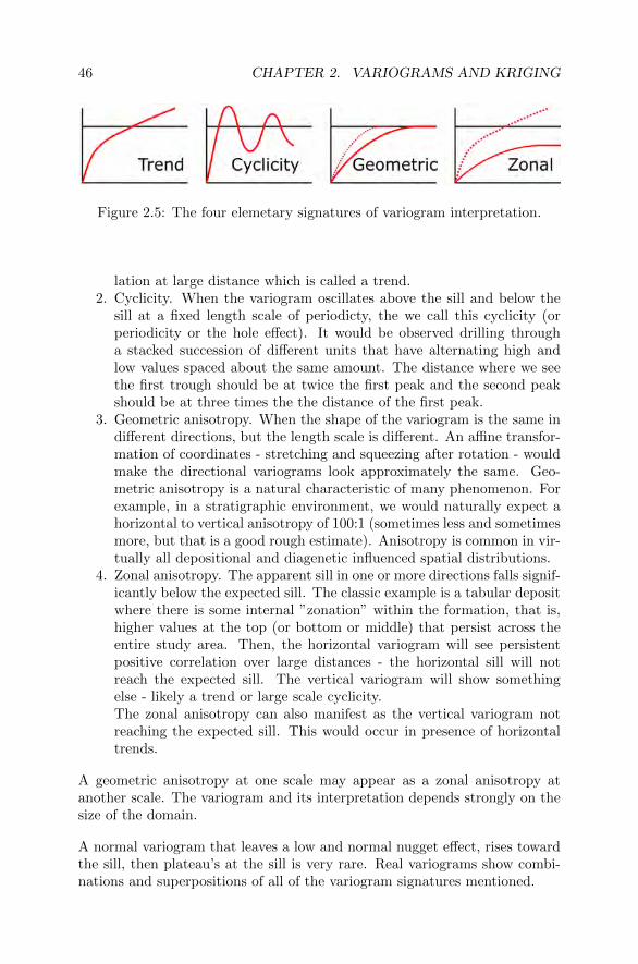
46 CHAPTER 2. VARIOGRAMS AND KRIGING
Figure 2.5: The four elemetary signatures of variogram interpretation.
lation at large distance which is called a trend.2. Cyclicity. When the variogram oscillates above the sill and below the
sill at a fixed length scale of periodicty, the we call this cyclicity (orperiodicity or the hole effect). It would be observed drilling througha stacked succession of different units that have alternating high andlow values spaced about the same amount. The distance where we seethe first trough should be at twice the first peak and the second peakshould be at three times the the distance of the first peak.
3. Geometric anisotropy. When the shape of the variogram is the same indifferent directions, but the length scale is different. An affine transfor-mation of coordinates - stretching and squeezing after rotation - wouldmake the directional variograms look approximately the same. Geo-metric anisotropy is a natural characteristic of many phenomenon. Forexample, in a stratigraphic environment, we would naturally expect ahorizontal to vertical anisotropy of 100:1 (sometimes less and sometimesmore, but that is a good rough estimate). Anisotropy is common in vir-tually all depositional and diagenetic influenced spatial distributions.
4. Zonal anisotropy. The apparent sill in one or more directions falls signif-icantly below the expected sill. The classic example is a tabular depositwhere there is some internal ”zonation” within the formation, that is,higher values at the top (or bottom or middle) that persist across theentire study area. Then, the horizontal variogram will see persistentpositive correlation over large distances - the horizontal sill will notreach the expected sill. The vertical variogram will show somethingelse - likely a trend or large scale cyclicity.The zonal anisotropy can also manifest as the vertical variogram notreaching the expected sill. This would occur in presence of horizontaltrends.
A geometric anisotropy at one scale may appear as a zonal anisotropy atanother scale. The variogram and its interpretation depends strongly on thesize of the domain.
A normal variogram that leaves a low and normal nugget effect, rises towardthe sill, then plateau’s at the sill is very rare. Real variograms show combi-nations and superpositions of all of the variogram signatures mentioned.
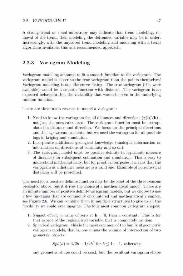
2.2. VARIOGRAMS II 47
A strong trend or zonal anisotropy may indicate that trend modeling, re-moval of the trend, then modeling the detrended variable may be in order.Increasingly, with the improved trend modeling and modeling with a trendalgorithms available, this is a recommended approach.
2.2.3 Variogram Modeling
Variogram modeling amounts to fit a smooth function to the variogram. Thevariogram model is closer to the true variogram than the points themselves!Variogram modeling is not like curve fitting. The true variogram (if it wereavailable) would be a smooth function with distance. The variogram is anexpected behaviour, but the variability that would be seen in the underlyingrandom function.
There are three main reasons to model a variogram:
1. Need to know the variogram for all distances and directions (γ(h)∀h) -not just the ones calculated. The variogram function must be extrap-olated in distance and direction. We focus on the principal directionsand the lags we can calculate, but we need the variogram for all possiblelags in kriging and simulation.
2. Incorporate additional geological knowledge (analogue information orinformation on directions of continuity and so on).
3. The variogram model must be positive definite (a legitimate measureof distance) for subsequent estimation and simulation. This is easy tounderstand mathematically, but for practical purposes it means that thevariogram as a distance measure is a valid one. Example of non-physicaldistances will be presented.
The need for a positive definite function may be the least of the three reasonspresented above, but it drives the choice of a mathematical model. There arean infinite number of positive definite variogram models, but we choose to usea few functions that are commonly encountered and mathematically simple,see Figure 2.6. We can combine them in multiple structures to give us all theflexibility we could ever imagine. The four most common variogram shapes:
1. Nugget effect: a value of zero at h = 0, then a constant. This is forthat aspect of the regionalized variable that is completely random.
2. Spherical variogram: this is the most common of the family of geometricvariogram models, that is, one minus the volume of intersection of twogeometric objects:
Sph(h) = 3/2h− 1/2h3 for h ≤ 1; 1, otherwise
any geometric shape could be used, but the resultant variogram shape
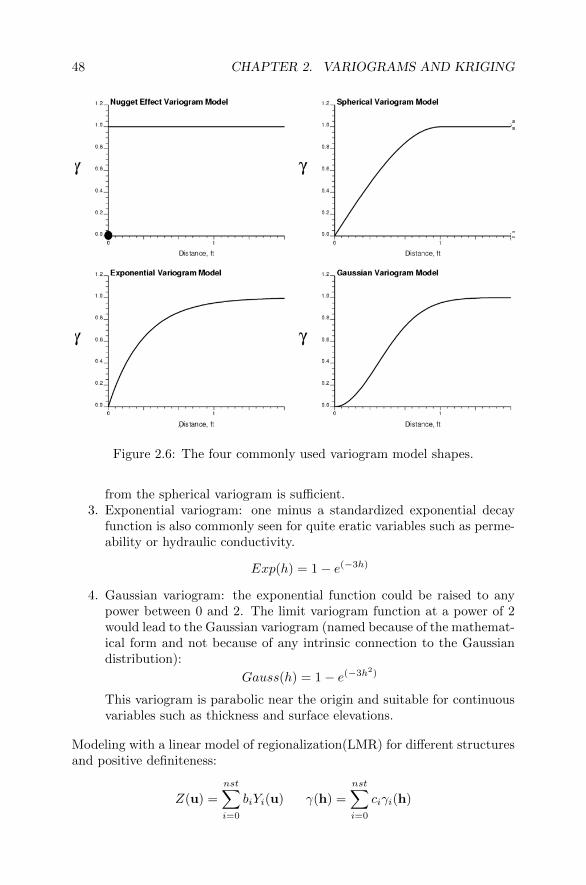
48 CHAPTER 2. VARIOGRAMS AND KRIGING
Figure 2.6: The four commonly used variogram model shapes.
from the spherical variogram is sufficient.3. Exponential variogram: one minus a standardized exponential decay
function is also commonly seen for quite eratic variables such as perme-ability or hydraulic conductivity.
Exp(h) = 1− e(−3h)
4. Gaussian variogram: the exponential function could be raised to anypower between 0 and 2. The limit variogram function at a power of 2would lead to the Gaussian variogram (named because of the mathemat-ical form and not because of any intrinsic connection to the Gaussiandistribution):
Gauss(h) = 1− e(−3h2)
This variogram is parabolic near the origin and suitable for continuousvariables such as thickness and surface elevations.
Modeling with a linear model of regionalization(LMR) for different structuresand positive definiteness:
Z(u) =
nst∑i=0
biYi(u) γ(h) =
nst∑i=0
ciγi(h)

2.2. VARIOGRAMS II 49
where i = 0 is nugget by convention. Each structure is defined by a shapeand six anisotropy parameters (three angles and three ranges - see Section1.1). The common shapes are described above. Considering that anisotropyis outside of variogram modeling, that is, it is specified per structure and itmodifies how the ”standardized isotropic distance” is calculated is relevant.
Variogram modeling amounts to picking a single (lowest) isotropic nuggeteffect, choosing the same number of variogram structures for all directionsbased on most complex directions, ensuring that the same sill parameter isused for all variogram structures in all directions, and allowing a differentrange parameter in each direction. A zonal anisotropy by setting a very largerange parameter in one or more of the principal directions.
An important topic in data poor areas of geostatistics is how to infer a vari-ogram in presence of sparese data. This is particularly relevant for variogrammodels in stratigraphic settings (petroleum reservoirs) with few wells. An es-tiamte of the zonal anisotropy and the geometric anisotropy of each structureis required.
There are software that mimics the iterative procedure performed by thevarigoram modeler, varying the different parameters that define a variogrammodel. The nugget effect, sill contributions, structure types and ranges, arefit to experimental variogram points in up to three directions simultaneously.The user can fix any subset of parameters. This is useful when the exper-imental variograms are well defined, but expert judgement is always to beconsidered.
A variogram model is specified by the number of structures, the nugget effectand (for each structure, the contribution, the shape and six anisotropy pa-rameters (three angles and three ranges). This is a very efficient compressionof the variogram information.
When there is doubt as to the most correct variogram model, then we consider(1) fidelity to the geology and the regionalized variable, (2) simplicity - simpleris better,
Variogram modeling is one of the most important steps in a geostatisticalstudy - all spatial inference depends on model of spatial variability / conti-nuity.
2.2.4 Exercise W2-2
The objective of this exercise is to gain experience and confidence in theexperimental calculation, interpretation and modeling of variograms for a
50 CHAPTER 2. VARIOGRAMS AND KRIGING
number of data sets.
1. Consider the directional horizontal and vertical variograms experimen-tally calculated in exercise W2-1 for bitumen with the oilsands.dat dataset. Fit the variograms. Tabulate your variogram model parameters andcomment on the uncertainty in the variogram model parameters.
2. Calculate, interpret and model the variogram of Au in skarn2d.dat (2-D).
3. Calculate, interpret and model the variogram of Au in Misima.dat (3-D).
2.3 Change of Support
2.3.1 Scales of Relevance
Change of support or volume variance relations relates to understanding whathappens at a larger scale given data and information at a smaller scale. The-oretically we may think of going down in scale, but the reality is that wedrill and observe variability at a small scale and we wish to predict what ishappening at a large scale of relevance. The data within reasonably station-ary domains provides a representative distribution through declustering anda representative variogram model. These statistical parameters relate to thescale of the data. Engineering considerations lead us to consider a selectivemining unit (SMU) that effectively represents a scale relevant for resourceand reserve assessment. The SMU scale (often denoted v) may be 4 to 9orders of magnitude larger than the scale of the data. We aim to predictwhat would be the representative distribution at that larger scale. This hassignificant consequences on resource and reserve estimation.
This is particularly important when there are no block data [45]. A theoreticalprediction of the change of support may all we have. The main reasons whywe consider this topic include (1) the resources and reserves we compute andreport are to reflect future mining and production, (2) there are no blockdata available early in the pre- and feasibility studies of a deposit, yet we areto represent that scale, (3) resources depend very strongly on the productionvolume and the inevitable smoothing that occurs as we consider statisticsrepresenting larger volumes, (4) we would like to know how much smoothing isacceptable in the application of conventional geostatistical (or any) estimationalgorithm, that is, we would often want to calibrate our resource estimationto anticipate future selectivity and provide unbiased block estimates, and (5)we would like a check on advanced simulation, UC, MIK and other predictionalgorithms.

2.3. CHANGE OF SUPPORT 51
The choice of an SMU (v) size is most relevant to open pit mining. It couldbe used for underground, but the less constrained selection of open pit ismore amenable to the underlying assumptions. The considerations include(1) the mining method - more flexible means smaller SMU size, (2) the miningequipment - smaller and more flexible means smaller SMU size, (3) blastingpractice - more agressive blasting with larger movement means larger SMUsize, (4) production sampling - more and better production sampling wouldimply a smaller SMU size, (5) visual control on the ore and the availabilityto support mine operations in the visual control - better control would im-ply a smaller SMU size, and (6) various other mining operations includingthe attention of management, mining at night near contacts, the bonus andincentivization schemes - as expected. The Lesson on change of support is auseful reference [31].
2.3.2 Volume-Variance Relations
The first key principle is additivity of variance expressed with dispersionvariances:
D2(v,A) = D2(v, V ) +D2(V,A) where |v| < |V | < |A|
A demonstration will be given that proves the additivity of variance. The keyprinciple is that the variance of composites within the stationary domain isequal to the variance of composites within the SMU volume and the varianceof SMU volumes within the domain. The variance of SMU volumes withinthe domain is a goal of volume variance relations.
The variance is often written as D2(·, A) = σ2, that is, the conventionalvariance of a variable is interpreted as the dispersion variance of point sampleswithin the domain.
Second, the volume averaged variogram is defined for two different volumes,perhaps at different locations:
γ(V, v) =1
|V | |v|
∫V
∫v
γ(x− y)dxdy
This could be used for general calculations including estimation variance andfor populating block kriging equations with data of different support. Forchange of support calculations, the volume average variogram of a volumewith itself, that is, of v if v = V is particularly important. It is the expectedvariance of points within the SMU volume:
γ(v, v) = D2(·, v)
Attempts have been made to solve the integrals requried for the volume av-eraged variogram, but the modern approach is to discretize the volume and
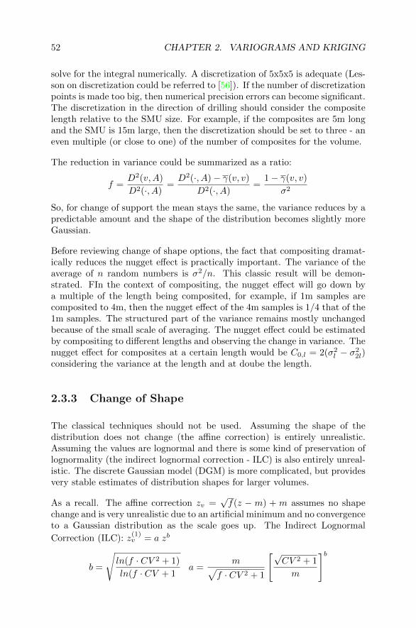
52 CHAPTER 2. VARIOGRAMS AND KRIGING
solve for the integral numerically. A discretization of 5x5x5 is adequate (Les-son on discretization could be referred to [56]). If the number of discretizationpoints is made too big, then numerical precision errors can become significant.The discretization in the direction of drilling should consider the compositelength relative to the SMU size. For example, if the composites are 5m longand the SMU is 15m large, then the discretization should be set to three - aneven multiple (or close to one) of the number of composites for the volume.
The reduction in variance could be summarized as a ratio:
f =D2(v,A)
D2(·, A)=D2(·, A)− γ(v, v)
D2(·, A)=
1− γ(v, v)
σ2
So, for change of support the mean stays the same, the variance reduces by apredictable amount and the shape of the distribution becomes slightly moreGaussian.
Before reviewing change of shape options, the fact that compositing dramat-ically reduces the nugget effect is practically important. The variance of theaverage of n random numbers is σ2/n. This classic result will be demon-strated. FIn the context of compositing, the nugget effect will go down bya multiple of the length being composited, for example, if 1m samples arecomposited to 4m, then the nugget effect of the 4m samples is 1/4 that of the1m samples. The structured part of the variance remains mostly unchangedbecause of the small scale of averaging. The nugget effect could be estimatedby compositing to different lengths and observing the change in variance. Thenugget effect for composites at a certain length would be C0,l = 2(σ2
l − σ22l)
considering the variance at the length and at doube the length.
2.3.3 Change of Shape
The classical techniques should not be used. Assuming the shape of thedistribution does not change (the affine correction) is entirely unrealistic.Assuming the values are lognormal and there is some kind of preservation oflognormality (the indirect lognormal correction - ILC) is also entirely unreal-istic. The discrete Gaussian model (DGM) is more complicated, but providesvery stable estimates of distribution shapes for larger volumes.
As a recall. The affine correction zv =√f(z − m) + m assumes no shape
change and is very unrealistic due to an artificial minimum and no convergenceto a Gaussian distribution as the scale goes up. The Indirect Lognormal
Correction (ILC): z(1)v = a zb
b =
√ln(f · CV 2 + 1)
ln(f · CV + 1a =
m√f · CV 2 + 1
[√CV 2 + 1
m
]b

2.3. CHANGE OF SUPPORT 53
z(2)v = z(1)v ·m
m1
provides for unrealistic shape change in upscaling, but is surprisingly usefulfor downscaling. For upscaling, the DGM more general and flexible.
The discrete Gaussian model may not be mathematically simple, but it ispowerful and very practical. Discrete Gaussian model (DGM) is based onHermite polynomials:
zv =
np∑p=0
φpHp(y)
Hp(y) =1√p!g(y)
dpg(y)
dyp
H0(y) = 1 H1(y) = −y H2(y) =1√2
(y2 − 1) H3(y) =−1√
6(y3 − 3y)
recursive equation for more:
Hp+1(y)− −1√p+ 1
yHp(y)−√
p
p+ 1Hp−1(y)
since the Hs are independent and standard the variance :
σ2 =
np∑p=1
φ2p
The diffusion and mosaic models for change of support (r values are deter-mined by trial and error):
φv,p = rpDφp φv,p = rMφp
The diffusion and mosaic models are characterized by:
γ1(h)√γ(h)
=C1√C
γ1(h)
γ(h)=C1
C
the barycentric model is in between the two. A measure of dissemination(1=D, 0=M) could be calculated:
β(h) =
(γ1(h)
C1− γ(h)
C
)/
(√γ(h)
C− γ(h)
C
)
φv,p = (βerpB + (1− βe)rB)φp
Most practitioners use the diffusion model and stop there. The use of themosaic model or a blend between the two (the barycentric model) may beuseful in certain cases. In practice, much upscaling is done by simulating ata high resolution, then averaging to larger volumes.

54 CHAPTER 2. VARIOGRAMS AND KRIGING
2.3.4 Exercise W2-3
The objective of this exercise is to learn how to scale variances with averagevariogram values and to review the common change of shape models. Av-erage variogram or gammabar values tell us the variance at any scale. Thediscretization required for stable numerical integration is a consideration.Average variogram values can be calculated between two disjoint volumes Vand v; however, classic histogram and variogram scaling requires the averagevariogram to be calculated for V = v, that is, for the same volume and itself.
1. Write a short review of the key theoretical results needed for variogramscaling: (1) the definition of the average variogram or average covari-ance, (2) the definition of the dispersion variance and the link to theaverage variogram, and (3) the additivity of variance.
2. Consider the Au variable from Misima.dat. Consider the variogrammodel from a previous exercise and a 10m by 10m by 10m block size.Create a plot with the average variogram versus discretization levelstarting with 1x1x1 and going to 6x6x6 in increments of 1.
3. Calculate the average variogram for block sizes of 5x5x5, 10x10x10,15x15x15, 25x25x15 and 50x50x15. Plot and tabulate (1) the averagevariogram versus block size, and (2) the block variance versus blocksize.
4. Consider a block size of a 10m by 10m by 10m. Calculate the scaleddistributions using the (1) affine, (2) indirect lognormal, and (3) discreteGaussian models. Plot the original Au histogram and all of the scaledhistograms. Comment on the results.
2.4 Kriging I
2.4.1 Linear Estimation
The context is to estimate a continuous rock property at an unsampled lo-cation using the available data in the domain. The data are denoted as aset:
n : z(uα) = zα, α = 1, . . . , n
statistical parameters have been inferred from the data including:
F (z), m, σ2, γ(h), and C(h) = σ2 − γ(h)
An unsampled location is denoted u�. A linear estimator at the unsampledlocation is written:
z∗� −m =n∑α=1
λα[zα −m]

2.4. KRIGING I 55
Figure 2.7: Classic sketch of kriging setup.
This assumes that the mean is stationary. The weights also depend on theunsampled location and should more properly be written λα(u�). We are notfitting a linear function to the data; we are computing the best linear estimateat each unsampled location. Taken together, the best estimates form a highlynon-linear surface. We could consider the residual from the mean Y = Z−mto simplify notation:
y∗� =
n∑α=1
λαyα
A good estimate could be calculated considering an inverse distance schemefor the weights:
λα =
(1
hα,�+0.5
)1.5∑nβ=1
(1
hβ,�+0.5
)1.5where hα,� is the standardized Euclidean distance (see Chapter 1) betweendata α and the unsampled location �. The small constant of 5% to therange is for stability and to mimic a small nugget effect. The power of 1.5has proven itself in cross validation studies although a higher power wouldlead to less smooth estimates. Considering global inverse distance would leadto a very reasonable (good) artifact free model. The goal of geostatistics tocalculate the best estimate.
There are many different criteria for the best estimate, but the quadratic lossL(e) = e2 is practical and unbiased (a recall of the theorem that ”among allestimators, the one that minimizes the squared error criterion is unbiased”will be reviewed in class. Minimizing mean squared error (MSE) is equivalentto maximizing the coefficient of determination R2. So, our definition of a bestestimate is one that minimizes error variance (MSE):
σ2E = E
{[Y ∗ − Y ]2
}

56 CHAPTER 2. VARIOGRAMS AND KRIGING
Considering absolute error leads to a bias. Introducing asymmetric penaltiesfor positive and negative errors would also lead to a bias. Risk aversion oropportunity seeking would be considered after predicting a local distributionof uncertainty (see Chapter 4).
2.4.2 Estimation Variance and Simple Kriging
The error variance can be expanded into three terms:
σ2E = E{Y ∗2� − 2Y ∗�Y� + Y 2
�}
= E
n∑α=1
n∑β=1
λαλβYαYβ − 2
n∑α=1
λαYαY� + Y 2�
=
n∑α=1
n∑β=1
λαλβCαβ − 2n∑α=1
λαCα� + σ2
the first term assesses the redundancy between the data - greater redundancyleads to higher error. The second term assesses the closeness between the dataand the unsampled location - the closer the data to the location being esti-mated leads to lower error. The third term is the stationary variance if thereare no nearby relevant data - a lower the stationary variance (homogeneousdomain) is better - everything else being equal.
The kriging equations are derived by taking the derivative of the error variancewith respect to each of the weights and setting them equal to zero:
δσ2E
δλα= 2
n∑β=1
λβCαβ − 2Cα� = 0, α = 1, . . . , n
n∑β=1
λβCαβ = Cα� α = 1, . . . , n
Solving these equations leads to a set of weights λα, α = 1, . . . , n that lead tothe minimum error variance estimate. This formalism was called Simple Krig-ing (SK) by Georges Matheron because of the fundamental essence/simplicity/lackof constraints. This form of estimator is also called the Kalman Filter, Opti-mal Interpolation and the Normal Equations in different contexts.
A demonstration in class at this point shows both cross validation and esti-mation on a grid. The estimates are smooth and converge to the mean farfrom data.

2.4. KRIGING I 57
2.4.3 Properties of Kriging and Ordinary Kriging
There are many remarkable properties of kriging that include:
• Kriging minimizes the error variance by construction: check the secondderivative of the error variance with respect to the weights - the result is2σ2 for all weights which is always positive - therefore we are minimizing.
• The variogram/covariance model for the minimization of error varianceis data driven (the experimental variogram points) and model driven(interpolation and extrapolation of the variogram to all distances). Thismakes it very hard to find an estimator with lower error variance.• Existence and uniqueness: provided there are no data at exactly the
same location and provided that we are using a positive definite covari-ance function C(h), the existence and uniqueness of the solution can beestablished.• Exactitude: the estimate z∗(u�) = z(uβ) if u� = uβ . This can be
shown easily from the existence and uniqueness of the kriging estimate.In these days of machine learning (ML) it is worth emphasizing thisproperty. ML estimates do not have the property of exactitude.• Block kriging: any shaped blocks can be kriged by discretizing them
with points, replacing the variance by the block variance σ2 = D2(v,A),and replacing the right hand side covariances by averages to the dis-cretization point locations: Cα� = C(α, v�).• Linearity of kriging: kriging can be applied with point and block data.
The block data could be any dimension or geometry - contiguous or not.Also, kriging a block directly with one system of equations or krigingeach discretization point, then averaging the point estimates leads toexactly the same result.• Kriging with kriged estimates gives the same estimate. Clearly the
minimized estimation variance or the kriging variance is lower, but theestimate is exactly the same. Consider kriging at any location u using ndata. Then, krige at location u′ with the same n data. Finally, krige atlocation u using the n data plus the estimate at u′. The final estimateand first estimate are exactly the same.• Simplified σ2
SK = σ2 −∑nα=1 λαCα�. The result of simple kriging and
the equation for the minimization of the error variance can be combinedand the minimized error variance shown with this simpler equation.• Kriged estimates are smoother than the random function, that is, V ar{Y ∗�} =σ2 − σ2
SK . The variance should be σ2, but it is reduced by the krigingvariance. The higher the kriging variance, the smoother the estimate.This makes sense since the kriging variance is higher when there arefewer nearby conditioning data.• Covariance reproduction, that is, E{YαY ∗�} = Cα�. Although the vari-
ance of the kriged estimates is too small, the covariance between allkriged estimates and all of the data is correct. This is sometimes used

58 CHAPTER 2. VARIOGRAMS AND KRIGING
as a basis for sequential simulation; however, a better basis would bethe recursive decomposition of the multivariate.
Ordinary kriging, discussed below, starts to impose constraints on the krigingestimator. Many of the properties listed above will only apply approximately,but the estimator may be improved.
Ordinary Kriging
The standard linear estimator:
z∗� −m =n∑α=1
λα[zα −m]
is reorganized to collect the terms applied to the mean:
z∗� =n∑α=1
λαzα +
[1−
n∑α=1
λα
]·m
The global mean m may be well known, but it may not be appropriate locally.The weight to the mean is constrained to equal zero while minimizing the errorvariance.
z∗� =n∑α=1
λαzα
minimize:n∑α=1
n∑β=1
λαλβCαβ − 2n∑α=1
λαCα� + σ2
subject to 1−n∑α=1
λα = 0
The Lagrange formalism is introduced, that is, to minimize f(x) subject tog(x) = 0, we minimize h(x)+µg(x) in an unconstrained fashion. In our case:
h(λ, µ) =n∑α=1
n∑β=1
λαλβCαβ − 2n∑α=1
λαCα� + σ2 + µ
[1−
n∑α=1
λα
]
Taking the n+ 1 derivatives and setting them to zero leads to:{ ∑nβ=1 λβCαβ − µ/2 = Cα�, α = 1, . . . , n∑nβ=1 λβ = 1
Georges Matheron called this ordinary kriging (OK). In presence of non-stationarity OK can outperform SK by not assigning any weight to the globalmean. OK also provides an opportunity for us to intervene in the smoothingof kriging by limiting the search.

2.4. KRIGING I 59
Figure 2.8: Data configuration for kriging exercise Question 3.
2.4.4 Exercise W2-4
The least squares formalism known as kriging in geostatistics is very impor-tant for geostatistical modeling.
1. Derive the estimation variance in terms of the covariance. Explainwhere the assumption of stationarity comes into the derivation.
2. Derive the simple kriging equations by taking the derivative of the es-timation variance with respect to the weights. Explain why the krigingweights do not depend on the data values and why this is important.
3. Consider the configuration below. The global mean is 1.3 thicknessunits and the variance is 0.2 thickness units2. Calculate the sim-ple kriging estimate and the simple kriging variance at the unsampledlocation given that the isotropic standardized covariance function isC(h) = exp(−3h/250). Show all steps clearly.

60 CHAPTER 2. VARIOGRAMS AND KRIGING

Chapter 3
Kriging and Simulation
The link between kriging and simulation is only strong through the multi-variate Gaussian distribution, but the history of geostatistics has made thegradual transition between these topics. That convention is followed, but theaim is to explain how simulation is truly different from kriging with somerandom perturbations.
3.1 Kriging II
3.1.1 Constrained Kriging
Ordinary and universal kriging where the mean is non-stationary [36, 42]:
m(u) =L∑l=0
alfl(u)
where the a coefficients are unknown and the fl terms are specified functionalsof location. By convention f0(u) = 1.
The path forward is to remove the mean from the estimator and enfoce un-biasedness:
E
{n∑α=1
λαz(uα)
}= E {z(u�)}
61

62 CHAPTER 3. KRIGING AND SIMULATION
The OK framework from the previous chapter is extended:{ ∑nβ=1 λβCαβ +
∑Ll=0 µl = Cα�, α = 1, . . . , n∑n
β=1 λβfl(uβ) = fl(u�), l = 0, . . . , L
Kriging with external drift (KED) is where one or more of the functionalscome from an external data source such as geophysics. KED is quite widelyused and recommended. Most implementations of UK where the functionalsare monomials of the coordinates are not recommended. The results are verysensitive to the search and can become unstable particularly in extrapolationwith a small search.
CCG paper 2006-119 documents and summarizes an interesting perspectiveon kriging with constraints (OK, UK/KT or KED). The perspective is basedon an understanding from the early days of geostatistics, but not well doc-umented. The perspective is that these constrained forms of kriging (OK,UK/KT or KED) are exactly equivalent to (1) estimation of the trend mod-eling parameters (the al terms above) by linear regression, then (2) simplekriging considering the mean estimated in the first step. This is an interestingperspective since it places all types of kriging as variants of simple kriging.
3.1.2 Primal and Dual Kriging
Kriging solves an optimization problem. The best weights are computed thatminimize the expected error variance. Most optimization problems can beexpressed in a primal form and a dual form. The development above is all inthe primal form. Expressing an optimization problem in a dual formalism isrevealing and potentially computationally advantageous.
Consider vectors of data, weights, right hand sides and the matrix for the lefthand side:
zT = [z1, z2, . . . , zn, 0, . . . , 0]
λT = [λ1, λ2, . . . , λn, µ0, . . . , µL]
kT = [C1�, C2�, . . . , Cn�, f0�, . . . , fL�]
K =
[Cαβfαl|fβl
0
]
Kriging can be expressed given this fundamental matrix notation. The esti-
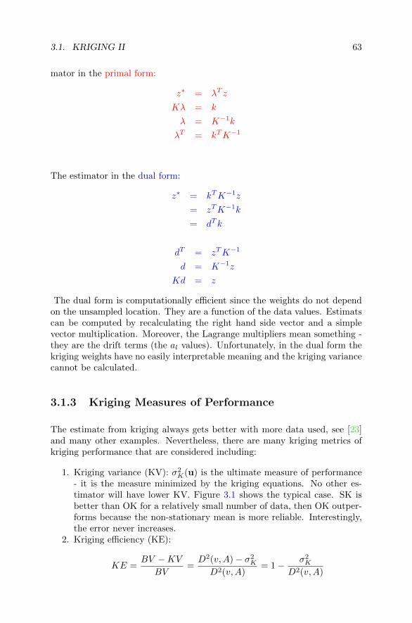
3.1. KRIGING II 63
mator in the primal form:
z∗ = λT z
Kλ = k
λ = K−1k
λT = kTK−1
The estimator in the dual form:
z∗ = kTK−1z
= zTK−1k
= dT k
dT = zTK−1
d = K−1z
Kd = z
The dual form is computationally efficient since the weights do not dependon the unsampled location. They are a function of the data values. Estimatscan be computed by recalculating the right hand side vector and a simplevector multiplication. Moreover, the Lagrange multipliers mean something -they are the drift terms (the al values). Unfortunately, in the dual form thekriging weights have no easily interpretable meaning and the kriging variancecannot be calculated.
3.1.3 Kriging Measures of Performance
The estimate from kriging always gets better with more data used, see [23]and many other examples. Nevertheless, there are many kriging metrics ofkriging performance that are considered including:
1. Kriging variance (KV): σ2K(u) is the ultimate measure of performance
- it is the measure minimized by the kriging equations. No other es-timator will have lower KV. Figure 3.1 shows the typical case. SK isbetter than OK for a relatively small number of data, then OK outper-forms because the non-stationary mean is more reliable. Interestingly,the error never increases.
2. Kriging efficiency (KE):
KE =BV −KV
BV=D2(v,A)− σ2
K
D2(v,A)= 1− σ2
K
D2(v,A)

64 CHAPTER 3. KRIGING AND SIMULATION
Figure 3.1: Typical example of the estimation variance versus the number ofdata used. Error goes down with the number of data used.
This is like a local R2 measure. It is also perfectly inversely related toKV and does not bring any new information - although it is dimension-less.
3. Statistical efficiency (SE): GSKV (u)σ2K(u)
. Efficiency in statistical regression
is related to how low the error variance is relative to the lowest it couldbe. The lowest possible is the global simple kriging variance.
4. Slope of regression (SR) will be developed more below, but it is lessthan one in OK with a limited search. Ideally, the SR is one, but weaccept it being less to avoid excessive smoothing.
5. Negative weight measure (NW)
nwm(u) =∑
all neg wts
|λα|n· 100
such that one weight of -0.1 in 10 would give a nwm of one. Negativeweights are not necessarily bad - they lead to local extrapolation inthe behaviour of the regionalized variable. Of course, large negativeweights and outliers certainly cause problems. In general, set negativeestimates to zero and move forward. If the number and magnitude ofthe negative estimates are significant, then it is likely that the variogramis inconsistent with the spatial distribution of the variable.
6. Weight to the mean (WM) - this is really only for SK. The more weightto the mean, the less the data are important.
Slope of regression:
z = a+ bz∗ b = ρσZσ∗Z

3.1. KRIGING II 65
b =Cov{z, z∗}σzσz∗
σZσZ∗
=Cov{Z,Z∗}
σ2z∗
= E{ZZ∗} −m2/E{Z∗Z∗} −m2
=E{∑nα=1 λαzαz} −m2
E{∑nα=1
∑nβ=1 λαλβzαzβ} −m2
=
∑nα=1 Cα�∑n
α=1
∑nβ=1 λαλβCαβ
for all variants of kriging. For SK :
σ2SK = σ2 −
n∑α=1
λαCα� (3.1)
= σ2 − 2
n∑α=1
λαCα� +
n∑α=1
n∑β=1
λαλβCαβ
b =σ2 − σ2
SK
σ2SK − σ2 + 2(σ2 − σ2
SK)=σ2 − σ2
SK
σ2 − σ2SK
= 1
For OK with one data:
b =C1�
σ2≤ 1
this shows that the slope is less than one and significantly less than one whenthe weight to the implicitly calculated local mean increases.
Metrics of performance should always be reviewed, but the results are un-satisfying. Kriging larger blocks is always better according to the measures,but are no different than smaller blocks in practice. The block size should bechosen for practical engineering reasons, adapting to geological boundariesand for computational considerations. Using more data is always better, butthis depends on the purpose of the estimate.
3.1.4 Exercise W3-1
The least-squares formalism known as kriging in geostatistics is very im-portant for geostatistical modeling. In this exercise you will apply differentkriging variants under cross validation and for kriging a grid. Data set to beused for mining is the gold grade in Misima.dat.
1. Run cross validation for simple kriging using the declustered mean with40 closest data using your variogram model. Plot a scatterplot betweenthe estimated and true values for each number of search data. Commenton the scatterplot, the mean error, mean squared error, variance of theestimates and correlation between the true values and estimates. Rerunthe cross validation with 4 data and compare.

66 CHAPTER 3. KRIGING AND SIMULATION
2. Now run cross validation for ordinary kriging with 40 closest data usingyour variogram model. Plot scatterplots and comment on your resultsas before. Comment on the differences in results between simple andordinary kriging. Rerun the cross validation with 4 data and compare.Pay particular attention to the conditional bias with ordinary kriging.
3. Estimate on a grid with simple point kriging and ordinary point krigingusing 40 samples. Plot slices through the models, histograms of theestimates and comment on the results.
4. Estimate on a grid with simple block kriging and ordinary block krigingusing 40 samples. Plot slices through the models, histograms of theestimates and comment on the results.
3.2 Kriging and Local Uncertainty
3.2.1 Kriging Paradigms
The four paradigms of kriging are differentiated by the goal of estimation:
• Visualization or implicit modeling of geology using distance functions orindicators: the goal for this type of estimate is an artifact free estimatethat is smooth and natural. A global search should be used if possible,ordinary kriging is preferred and the dual formalism is also preferredfor computational efficiency.• Final estimate when no (or very little) additional data is coming avail-
able to help the design or decision: the goals for this type of estimate isto have the best resolution possible (down to 1/4 of the data spacing),avoid any conditional bias and get the best estimate possible - minimumMSE and minimum Type I/II errors. The smoothing of the estimate isof no consequence. A reasonably large search, ordinary kriging, pointsor small block estimation with 25 (2-D) to 50 (3-D) data.• Interim estimate - long range resource estimates awaiting more data in
the future: the goal is to match what will be mined in the future andto avoid excessive smoothing of the estimates. Conditional bias is of noconsequence to this type of estimate. Ordinary kriging is used with alimited search. Volume variance relations are often used to predict thevariance or grade tonnage curve that would be encountered in the futureand to help choose a limited number of data for the kriging. The searchis set fairly large, but the number of data are calibrated for the SMUv variance D2(v,A), that is, the variance of the estimates is matchedto the anticipated variance (or the grade tonnage curve at the chosencutoff. The estimate is not a good final estimate, but the purpose is tomatch future production - not provide the best local estimate.

3.2. KRIGING AND LOCAL UNCERTAINTY 67
• Probabilistic prediction for uncertainty calculations or simulation: thegoal is accuracy and precision of the predicted probabilities, artifactfree estimation and consistency with the underlying random function.For Gaussian variables, simple kriging (SK) should be used with a largesearch and a large number of data: 25 (2-D) to 50 (3-D) data. For indi-cators, OK is used with a consistent large search across all thresholds.
The key is the difference between a final estimate and an interim estimateanticipating the information effect. Some more details on setting the krigingplan can be found in the Lesson [20].
The block size is an important consideration in kriging. The natural size isabout 1/4 data spacing. Estimating blocks smaller than that does not improvethe delimitation of boundaries between high and low values. Larger blocksmake boundaries fuzzy and imprecise. Small blocks or even points should beused for final estimates, then boundaries can be traced between zones of highand low values that reflect the selectivity of the operation. Final selectivityis better represented by boundaries than by large blocks. The concept of anSMU is for long range interim resource estimation and not final estimation.
The number of data to use in kriging is another consideration. Interestingly,according to all metrics of performance (MSE, R2, Type I/II errors,...) moredata is always better. The advice given above is for 25 (2-D) to 50 (3-D)since the improvement past that number is negligible, yet the computer costkeeps increasing. The close data receive almost all of the weight in krigingand increasing the number beyond these values do not change the estimatesmuch. In fact, global kriging with all of the data, particularly in the dualformalism, is a very useful approach to estimation.
The search radius is often set to the variogram range. Unfortunately, thevariogram range is an ambiguous parameter since the variogram often ap-proaches the sill in an asymptotic manner. The search range should be setfairly large, then the number of data actually used in the kriging restrictedby the maximum per drill hole (2 to 3 - to avoid the string effect and sub-optimal estimates), maximum per octant (4 to 8 - to avoid artifacts causedby clustered data) and the absolute maximums of 25 to 50. The final esti-mates can be clipped by a maximum data spacing, that is, a high resolutiondata spacing model should be constructed and blocks that are in areas witha too-large data spacing should be set to missing.
There is no theory for multiple pass searches. Some practitioners like the useof multiple pass searches to avoid excessive smoothing, build in classificationcriteria and avoid estimating too far. The preference of this author is tomake the best estimate possible for the paradigm under consideration, thenclip and classify according to a high resolution data spacing model.
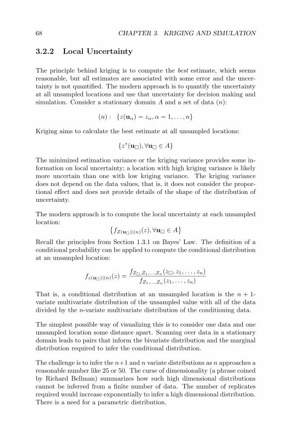
68 CHAPTER 3. KRIGING AND SIMULATION
3.2.2 Local Uncertainty
The principle behind kriging is to compute the best estimate, which seemsreasonable, but all estimates are associated with some error and the uncer-tainty is not quantified. The modern approach is to quantify the uncertaintyat all unsampled locations and use that uncertainty for decision making andsimulation. Consider a stationary domain A and a set of data (n):
(n) : {z(uα) = zα, α = 1, . . . , n}
Kriging aims to calculate the best estimate at all unsampled locations:
{z∗(u�),∀u� ∈ A}
The minimized estimation variance or the kriging variance provides some in-formation on local uncertainty; a location with high kriging variance is likelymore uncertain than one with low kriging variance. The kriging variancedoes not depend on the data values, that is, it does not consider the propor-tional effect and does not provide details of the shape of the distribution ofuncertainty.
The modern approach is to compute the local uncertainty at each unsampledlocation: {
fZ(u�)|(n)(z), ∀u� ∈ A}
Recall the principles from Section 1.3.1 on Bayes’ Law. The definition of aconditional probability can be applied to compute the conditional distributionat an unsampled location:
fz(u�)|(n)(z) =fZ�,Z1,...,Zn(z�, z1, . . . , zn)
fZ1,...,Zn(z1, . . . , zn)
That is, a conditional distribution at an unsampled location is the n + 1-variate multivariate distribution of the unsampled value with all of the datadivided by the n-variate multivariate distribution of the conditioning data.
The simplest possible way of visualizing this is to consider one data and oneunsampled location some distance apart. Scanning over data in a stationarydomain leads to pairs that inform the bivariate distribution and the marginaldistribution required to infer the conditional distribution.
The challenge is to infer the n+1 and n variate distributions as n approaches areasonable number like 25 or 50. The curse of dimensionality (a phrase coinedby Richard Bellman) summarizes how such high dimensional distributionscannot be inferred from a finite number of data. The number of replicatesrequired would increase exponentially to infer a high dimensional distribution.There is a need for a parametric distribution.

3.2. KRIGING AND LOCAL UNCERTAINTY 69
There are an infinite number of parametric distributions for univariate ran-dom variables. Some of these are based on a probabilistic generating mech-anism, but most are based on satisfying the requirements of a CDF (non-decreasing between 0 and 1) or a PDF (non-negative and integrates to 1).There are also an infinite number of parametric distributions for independentvariables. The multivariate distribution of n independent variables is simplythe product of the univariate distributions. In geostatistics, the n+1 locationsunder consideration are related together spatially through the underlying ge-ological processes that led to the present day distribution. The options closein and there is only one parametric multivariate distribution that is math-ematically tractible with arbitrarily correlated variables. The multivariateGaussian (MG) distribution is unique in mathematics and probability.
3.2.3 MultiGaussian Kriging
The multivariate Gaussian distribution is truly unique and widely exploitedin statistics and geostatistics. The setup of MG including back transform willbe presented. This was developed by Verly in the 80s [59]. The multivariateGaussian distribution has remarkable properties:
f (y;µ,Σ) =1(√
2π)d |Σ|1/2 e−(y−µ)TΣ−1(y−µ
2
The value y is a vector position in a d dimensional space. There are twoparameters: (1) µ - a d dimensioned vector of mean values in each coordi-nate/dimension, and (2) Σ - a dxd dimensioned matrix of variance-covariancevalues between each coordinate/dimension. As explained in Chapter 1, thegenerating mechanism of this distribution is summarized by the central limittheorem - the sum of many independent identically distributed variables tendsto a Gaussian distribution. Regardless of whether our variables satisfy thisgenerating mechanism, we adopt this distribution because of its remarkableproperties.
The first of many remarkable properties is that all lower c < d distributionsare also Gaussian if the d-variate distribution is Gaussian. To the extreme,the univariate distribution of each of the d variables must be Gaussian. Allbivariate distributions are bivariate Gaussian and so on. The shape of anymarginal or conditional distribution is Gaussian - all we need is the meanvector and variance-covariance matrix to define it completely.
The second remarkable property is that all conditional mean values are linearfunctions of the conditioning data. In many cases, a linear estimate is adoptedfor simplicity, but in the case of the multivariate Gaussian distribution, alinear combination of conditioning data is the conditional mean.

70 CHAPTER 3. KRIGING AND SIMULATION
A third remarkable property of the multivariate Gaussian distribution is thatthe conditional variance (of any conditional distribution) does not depend onthe conditioning data - the conditional variance only depends on the variance-covariance structure between the conditioning data and the variable underconsideration.
These properties all lead to the final and most important remarkable propertyof the multivariate Gaussian distribution. The conditional mean and variance(covariance) values for a multivariate Gaussian distribution are given by thenormal equations that are known as simple kriging (SK) in geostatistics.
mc =n∑α=1
λαyα
σ2c = σ2 −
n∑α=1
λαCα,�
n∑β=1
λβCαβ = Cα� α = 1, . . . , n
This is an endless source of confusion for classically trained geostatisticians.The belief is that simulation and uncertainty evolved from kriging. That isnot true. The normal equations (referred to as SK above) are the analyticalsolution arising from the MG distribution. If the random variable is multi-variate Gaussian, then any conditional distribution is (1) Gaussian in shape,(2) a mean value given by a linear combination of the conditioning data, and(3) a conditional variance that depends on the variace-covariance structureof the data. Conditional distributions are easily calculated if the multivariatedistribution is multivariate Gaussian.
The premise of modern geostatistics is that two assumptions are required: (1)a careful choice of stationarity - a geological population of data and unsam-pled locations that belong together, and (2) a normal score transform of allthe variables in the stationary domain. Then, all locations within the station-ary domain are assumed to be multivariate Gaussian. All local conditionaldistributions are calculated by the normal equations. The local Gaussiandistributions must be back transformed.
The back transformation of a local distribution must be accomplished througha quantile-quantile transformation via the global distribution. Most of us wishfor a transformation that would consider only the mean and variance, but theentire shape of the local distribution must be informed. This involves defininga set of probability values randomly or by a regular discretization (preferredat this point). The L probability values are defined by:
pl =l
L+ 1, l = 1, . . . , L using L = 200

3.2. KRIGING AND LOCAL UNCERTAINTY 71
Then, considering the local Gaussian distribution, the original units distribu-tion is defined by the back transformed quantiles:
zl = F−1(G(G−1(pl) · σc(u) +mc(u)
))l = 1, . . . L ∀u
The back transformation is sketched in Figure 3.2 where two local conditionaldistributions are back transformed. In Gaussian units, the red and the greendistributions have nearly the same variance, but the distributions in originalunits are quite different due to the skewness of the original units distribution.Given zl, l = 1, . . . L, any summary measure of uncertainty can be computed.The mean, variance, probability to be within an interval of the mean, anyother probability values can be computed from these values. The local valuescould be corrected by volume variance relations; however, the local change ofsupport is not the same everwhere as the global change of support.
There are three key ingredients for this approach to work. First, the sta-tionary domain and data must be geologically coherent and belong together.Second, the distribution F (z) that represents the stationary domain must betruly representative of the stationary domain. Finally, the variogram modelof the normal scores that inform the covarnace model must also be represen-tative of the stationary domain.
3.2.4 Exercise W3-2
The objective of this exercise is to become familiar with how kriging can beused to quantify uncertainty without resorting to simulation. Concepts herewill be useful for understanding Gaussian simulation algorithms.
Recall the data configuration used previously for kriging by hand (Figure ??).For this exercises, consider that the thicknesses were found to fit an exponen-tial distribution with a mean of 1 thickness unit. The cumulative distributionfunction of the exponential distribution is given as:
F (x;λ) = 1− exp(−λx), when x > 0 and 0 otherwise
where λ is the inverse of the mean. We are interesting in the uncertainty inthickness at the unsampled location shown.
1. Transform the thickness values to Gaussian units.2. Calculate the conditional mean and conditional variance at the unknown
location in Gaussian units.3. Back transform 99 evenly spaced percentiles (0.01, 0.02, . . . , 0.99) to es-
tablish the local conditional distribution at the unsampled location inunits of thickness. Plot the distribution and comment on the shape.
4. Using these back-transformed values, calculate the mean thickness anda 90% probability interval for the thickness at the unsampled location.
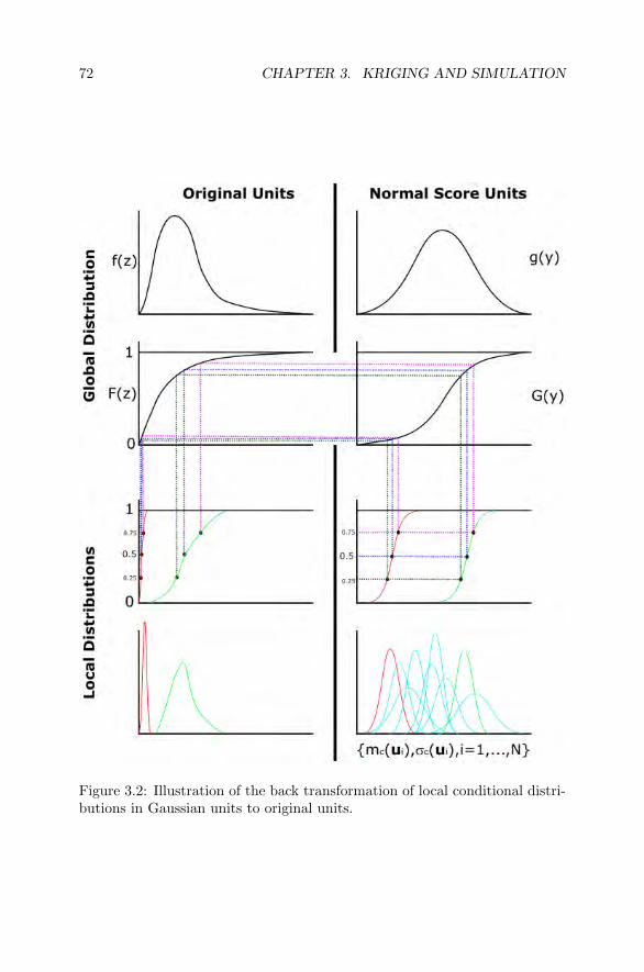
72 CHAPTER 3. KRIGING AND SIMULATION
Figure 3.2: Illustration of the back transformation of local conditional distri-butions in Gaussian units to original units.

3.3. SIMULATION I 73
Figure 3.3: Schematic illustration of a stope, SMU and pushback with somediscretization points.
3.3 Simulation I
3.3.1 Monte Carlo Simulation
Local uncertainty is useful for drill hole planning and placement, but we areoften interested in the uncertainty that involves multiple values/locations atthe same time. We are often interested in uncertainty in a value that de-pends on many locations at the same time: a stope, an SMU, a push back,the production for a month (quarter or year), the entire life of mine (LOM)resources, see Figure 3.3 for a sketch. A challenge is to convert local uncer-tainty to uncertainty in many locations at the same time. Many locationsimplies thousands to millions.
Monte Carlo simulation is the novel and unassailable technique to solve thisproblem. A classic reference with historical perspective is [30]. On reflection,there is no other approach to transfer uncertainty from a point scale to largerscale. Think about the curse of dimensionality.
Consider n input variables that are arbitrarily correlated and a response thatis some function of all n at the same time. There is uncertainty in each of then variables that must be transferred through to the response. see Figure 3.5.An evident approach is to discretize all n input variables by some number (10to 100) and compute the response for the combinatorial of input variables.The problem is that that the number is nearly infinite. A full combinatorialof all options is not possible.
Sampling in a systematic manner would not be reasonable. Sampling all lowvalues for every variable or all high values for every variable would lead tohighly improbable results. Sampling the median of all variables is unlikelyto be the median of the response. The variability matters and the variabilitymay lead to a systematic change in the results. Examples based on cablelength (see Figure 3.6) and flow simulation will be discussed.
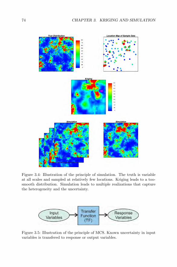
74 CHAPTER 3. KRIGING AND SIMULATION
Figure 3.4: Illustration of the principle of simulation. The truth is variableat all scales and sampled at relatively few locations. Kriging leads to a too-smooth distribution. Simulation leads to multiple realizations that capturethe heterogeneity and the uncertainty.
Figure 3.5: Illustration of the principle of MCS. Known uncertainty in inputvariables is transfered to response or output variables.
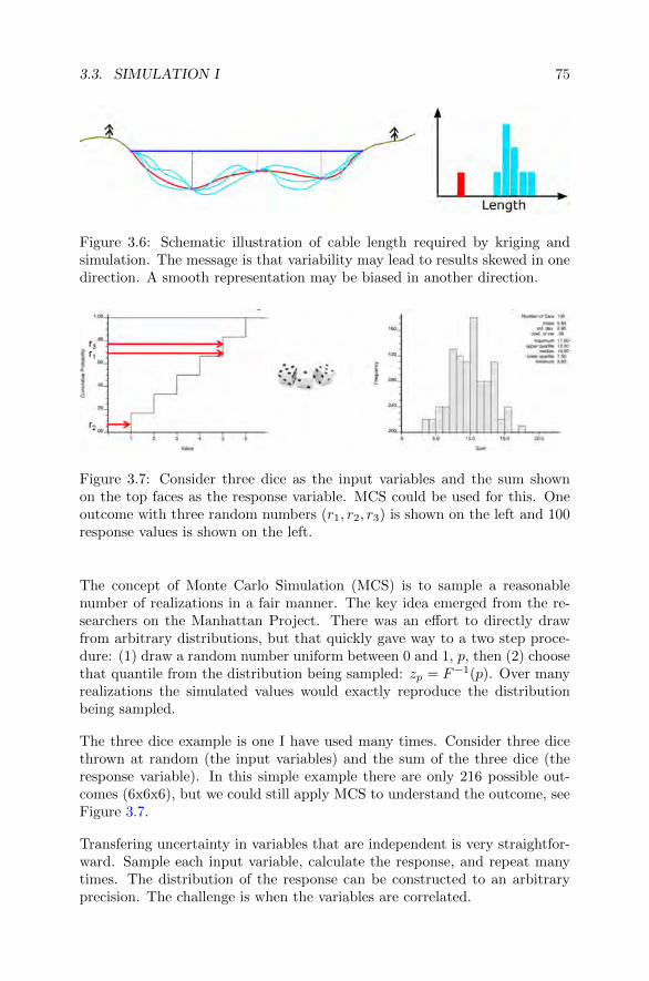
3.3. SIMULATION I 75
Figure 3.6: Schematic illustration of cable length required by kriging andsimulation. The message is that variability may lead to results skewed in onedirection. A smooth representation may be biased in another direction.
Figure 3.7: Consider three dice as the input variables and the sum shownon the top faces as the response variable. MCS could be used for this. Oneoutcome with three random numbers (r1, r2, r3) is shown on the left and 100response values is shown on the left.
The concept of Monte Carlo Simulation (MCS) is to sample a reasonablenumber of realizations in a fair manner. The key idea emerged from the re-searchers on the Manhattan Project. There was an effort to directly drawfrom arbitrary distributions, but that quickly gave way to a two step proce-dure: (1) draw a random number uniform between 0 and 1, p, then (2) choosethat quantile from the distribution being sampled: zp = F−1(p). Over manyrealizations the simulated values would exactly reproduce the distributionbeing sampled.
The three dice example is one I have used many times. Consider three dicethrown at random (the input variables) and the sum of the three dice (theresponse variable). In this simple example there are only 216 possible out-comes (6x6x6), but we could still apply MCS to understand the outcome, seeFigure 3.7.
Transfering uncertainty in variables that are independent is very straightfor-ward. Sample each input variable, calculate the response, and repeat manytimes. The distribution of the response can be constructed to an arbitraryprecision. The challenge is when the variables are correlated.
76 CHAPTER 3. KRIGING AND SIMULATION
3.3.2 Simulating Correlated Variables
The concept of MCS is well suited to independent variables. Simulatingmany dependent variables is essential in geostatistics. There may be a varietyof mathematically clever solutions, but for understanding purposes, there isnothing that comes close to sequential simulation.
Consider MCS from a bivariate distribution of two correlated variables. TheZ1 value and the Z2 value cannot be drawn independently - any direct orinverse relationship would not be respected. If the same random number isused for both the Z1 and Z2 value, then the relationship would be a perfectdirect relationship and the scatter would not be respected. As above, recallthe principles from Section 1.3.1 on Bayes’ Law. The definition of a condi-tional probability can be applied to compute the conditional distribution atan unsampled location:
fZ2|Z1(z) =
fZ1,Z2(z1, z2)
fZ1(z1)
leading to:fZ1,Z2
(z1, z2) = fZ2|Z1(z) · fZ1
(z1)
The path forward is clear. Regardless of the structure between Z1 and Z2,the bivariate distribution can be decomposed into a sequence of two univari-ate distributions (recall Figure 1.19 for an example): (1) draw z1 from themarginal distribution of Z1, then (2) draw z2 from the conditional distributionof Z2|Z1 = z1. Any bivariate distribution would be preserved by this proce-dure. The order of the variables does not matter - z2 could be drawn first,then z1. The key point is that after drawing one variable it must conditionthe next.
This concept can be generalized to any number of variables. Consider Nvariables:
P (A1, . . . , AN ) = P (AN |A1, . . . , AN−1)
P (A1, . . . , AN−1)
= P (AN |A1, . . . , AN−1)
P (AN−1|A1, . . . , AN−2)
P (A1, . . . , AN−2)
...
In practice, the n data are considered as samples already drawn from themultivariate distribution. Simulation starts at n+1 and proceeds to N . Also,in practice, as the number of conditioning data increases the number that areactually considered must be limited. A Markov screening like assumption

3.3. SIMULATION I 77
is considered where the nearby values that would influence the conditionaldistribution are used (the 25 to 50 data mentioned previously). In practice,the derivation of a conditional distribution using 25 to 50 data remains achallenge.
3.3.3 Sequential Gaussian Simulation (SGS)
SGS may not stand the test of time as the most efficient implementation, butfor understanding and for flexibility - it is unparalleled. A review of SGS ispresented.
Consider the sequential simulation paradigm presented in the previous sec-tion. Consider also that the regionalized variable under consideration hasbeen transformed to normal scores, assumed multivariate Gaussian, and fullyparameterized by a stationary assumption for the mean and a normal scoresvariogram model that informs the covariance structure. Then, the samemethodology as used for MG kriging could be used to derive the conditionaldistribution at each step in the sequential simulation approach. Consider thefollowing steps:
1. Establish a representative distribution FZ(z) using the best declusteringand debiasing availble. The data are normal score transformed usingthis distribution. The mean is assumed stationary here - a trend modelcould intervene in the transformation, but that will be seen in the nextchapter.
2. Calculate, interpret and model a variogram of the normal score trans-formed data. This provides the variance/covariance values needed forthe multivariate Gaussian distribution.
3. Define a sequence or path through all of the locations to be simulated.This could be any path, but a random path is often considered to avoidany artifacts in the simulated realization.(a) Calculate the conditional distribution at the current location con-
sidering all original data and previously simulated values - limitour consideration to the nearest 25-50 values. This amounts toapplying SK to the nearby data.
(b) Draw a random value from the conditional distribution. Draw arandom Gaussian deviate and consider the conditional mean andvariance from the previous step.
(c) Add the simulated value to the set of data and continue to thenext location.
4. Repeat the step above as many times as required for a reasonable num-ber of realizations (200?).
5. Back transform all normal score values to original units.

78 CHAPTER 3. KRIGING AND SIMULATION
This procedure is well established and known as Sequential Gaussian Simu-lation (SGS). There are alternatives based on unconditional simulation andconditioning by kriging, but they amount to the exact same result - real-izations from a multivariate Gaussian distribution. There are computationalconsiderations, but theoretically the results are the same. SGS is easy tounderstand.
3.3.4 Exercise W3-3
Simulation is the only method for the joint quantification of uncertainty be-tween multiple variables at multiple locations. This exercise will use the samedata sets used for the kriging exercise. Consider Au in the Misima data.
1. Using the declustered distribution, normal score transform variable toGaussian units. Calculate and model directional variograms for thenormal score transformed variable. Use the directions and models fromthe kriging assignment as a starting point and modify as appropriate.
2. Run point simple kriging of the normal score variable with a mean ofzero, a search up to the variogram range and up to 40 data. Plot someslices of the simple kriging estimates and the simple kriging variance.
3. Use sequential Gaussian simulation to simulate 200 realizations of thenormal score variable. Do not have the simulation program transformthe data; use your normal score transformed values. Plot slices throughthe first two realizations and comment on the results. Average all 200realizations on a block-by-block basis to calculate the e-type estimateand variance. Plot maps of the e-type mean and variance and comparewith the point simple kriging results from Question 2.
4. Use sequential Gaussian simulation to simulate 200 realizations lettingthe program transform and back transform. Average all realizations ona block-by-block basis to calculate the e-type mean and variance. Plotslices through the first two realizations, e-type mean and variance inoriginal units.
3.4 Simulation II
3.4.1 Implementation of SGS
All Gaussian simulation algorithms have the same prerequisites. Any largescale trend must be modeled and the variable detrended before proceedingwith simulation. The data must be correctly positioned and outliers must bemanaged. Simulation is more robust with respect to outliers than kriging,

3.4. SIMULATION II 79
but the tails of the distribution are reproduced by simulation and outliersmust be managed carefully.
Another consideration is that simulation assigns values at the scale of thedata. The values are averaged to blocks after simulation. There should be 9values or so (see Lesson on discretization) per block for reliable block values.The number of discretization points may need to be greater if the propertybeing simulated is non-linear and a physics based upscaling is being applied.
All Gaussian simulation algorithms require the data to be transformed to astandard normal distribution. The reference distribution for transformationmust be truly representative of the domain under consideration. Declusteringand debiasing are applied, see Chapter 1.
The number of data used to condition the local distributions as simulationproceeds must be sufficient. The 25 in 2-D and 50 in 3-D rules expressed aboveshould be considered. The default in legacy SGS codes (like the GSLIB sgsimprogram) may be set low for testing/speed. The number of data should notbe compromised.
The sequence of visiting the grid nodes for simulation is random to avoidany artifacts. Not completely random - a multiple grid search is a good idea.Simulating a coarse grid, then an intermediate grid, then the final grid helpsto enforce long range variogram structure - especially zonal anisotropy. Theorder within each grid is random.
Sequential Gaussian Simulation (SGS) works well if sufficient data are usedin the path. Some published examples showing SGS does not work considerimplementation choices that are poor: no surprise that a technique does notwork well if incorrectly applied. Although SGS can work well, an alternativeto Gaussian simulation is to (1) generate unconditional realizations, then (2)condition by kriging. Unconditional simulation can be very fast with turningbands, spectral techniques and perhaps moving average (convolution) tech-niques depending on the variogram. Then, conditioning by kriging can befast if global dual kriging can be applied. The results of this two-step proce-dure may be more computationally efficient than SGS, but the multivariatedistribution being sampled is the same if parameterized the same.
3.4.2 Checking Local Uncertainty
Local estimation is straightforward - we look to minimize the mean squarederror (MSE) and maximize the coefficient of determination (R2) with an unbi-ased estimator. In the context of simulation or the prediction of uncertainty,the local expected value should be checked against the true values in a clas-
80 CHAPTER 3. KRIGING AND SIMULATION
sical estimation cross validation mode. There may be systematic biases thatare masked by the variability/uncertainty that are caught by checking theexpected value.
In the case of uncertainty, accuracy and precision are important. [15] and haveto be checked in addition to the expected value. Accuracy is the correctnessof the probabilities, that is, do the proportions meet the predicted meaning.Consider some probability intervals, e.g., pi = 0.1, 0.2, . . . , 0.9, then:
plowi =1− pi
2phighi =
1 + pi2
pi =Number in (plowi , phighi ]
Total Number
The probabilities are accurate if pi ≥ pi∀i. Categorical variables are checkedby the probability ± a tolerance.
This general approach to check accuracy applies to continuous or categoricalvariables and parametric or non-parametric distributions. In the context ofGaussian distributions the checking is more straightforward since the localdistributions are fully defined by a conditional mean and conditional vari-ance. There is no need to simulate to assess the local uncertainty. Recallthat simulation is to transfer local uncertainty to multilocation or multivari-ate uncertainty - the local uncertainty is defined analytically in a multivariateGaussian context. The accplt ns program is designed especially for normalscores (Gaussian) values. A schematic of an accuracy plot is shown on Fig-ure 3.8. Note that experimental points should fall on (or above) the 1:1 linefor accuracy.
Accuracy is the number one consideration in checking uncertainty. If dis-tributions of uncertainty are not accurate, then they are not useful. Onceaccuracy is achieved we turn our attention to precision. Precision is the nar-rowness of the uncertainty. Everything being equal we would prefer moreprecise distributions. Considering the global distribution at each locationwould be accurate, but not precise. Considering a single estimate at eachlocation would be precise (no variability at all), but not accurate. As men-tioned, we must ensure accuracy and then seek the most precise distributionspossible.
Measures of precision for continuous and categorical variables:
Pcont =1n
∑ni=1 σ
2c,i
σ2
Pcat =1n
∑ni=1Hc,i
Hmax

3.4. SIMULATION II 81
Figure 3.8: Illustration of an accuracy plot. The experimental points shouldfall on the 1:1 45 degree line. Points above the line are accurate, but needlesslyhigh variance. Points below the line are inaccurate.
The checking software or a custom piece of code should be used to calculatethe precision. If the entire workflow is designed correctly, then the practitionerwill be naturally led to accurate distributions that are as precise as possible.It should not be possible to randomly perturb the parameters of uncertaintycalculation and get to better results.
As more data is acquired, predictions of uncertainty should stay accurateand become more precise. At times, uncertainty increases with more datadue to a change in the conceptual geological model. This should not happenoften. Parameter uncertainty early on should be large enough to capture thisuncertainty.
3.4.3 Checking Simulated Realizations
Checking and validating the results of numerical modeling should be consid-ered to the greatest extent possible. There are minimum acceptance criteriathat have been documented. Consider the Lesson [19] and other tradecraftdetails.
The results of simulation must always be checked carefully - regardless of howwell the practitioner understands the theory and software for simulation. Realgeology is complex and unlikely to exactly follow our implicit assumptions.A checklist:
• Data reproduction - all data should be reproduced at their locations.

82 CHAPTER 3. KRIGING AND SIMULATION
Some differences are expected when the simulated locations do not coin-cide with the data locations or there are dense conditioning data relativeto the spacing of the simulated nodes.• No visual artifacts - although visual inspection is not definitive, care-
ful visual inspection of the realizations can reveal numerical artifacts,edge effects, high grades in known low grade areas (and vice versa),unrealistic continuity or randomness and other issues. The pattern ofvariability away from the drill holes should look like at the drill holes.• Cross validation in estimation and uncertainty mode - as described in
the previous section should be considered. The expected values shouldbe unbiased and the uncertainty should be accurate and precise.• Statistics reproduction (F, γ, ρ, . . .) - the histogram, variogram and other
statistical parameters such as the correlation coefficient to secondarydata other simulated variables should be reasonably reproduced. Thereference declustered distribution is important. The variograms of thesimulated realizations should be closer to the experimental points thanthe fitted model. An example of statistical reproduction is shown inFigure 3.9. In presence of parameter uncertainty, check against basecase.• Swath plots - considering the average properties in principal directions
are used to check reproduction of trends and the data. The ”swaths”are perpendicular to the direction vector with tolerance. The averageof the data in each swath is compared to the realizations. Figure 3.10shows an example.• Average of many realizations equal to kriging - simulation after all does
not bring new information to the spatial distribution. Realizations re-flect reasonable variability and quantify uncertainty, but kriging pro-vides a solid estimate of the expected value. The correlation betweenthe average of many realizations and kriging should exceed 0.97.• Reconciliation with production data - this is always the gold standard.
Researchers at a university are developing algorithms and are not work-ing at a mine. Unsurprisingly, they do not ”talk to their metallurgists”since there are none. At a real operation, however, it is essential thatthe resource model be reconciled with short term models and with pro-duction from the mill.
Correct to kriging if required:
z(u; l) = z(u; l) · zOK(u)1L
∑z(u; l)
This correction is particularly useful if a trend model is not being consideredand a good ordinary kriged model captures the trend.
Correct the histogram (perhaps iteratively):
z1(u; l) = F−1rep (FL(z(u; l)))

3.4. SIMULATION II 83
Figure 3.9: Illustration of statistics reproduction for the histogram and vari-ogram. These results show excellent reproduction.
Figure 3.10: Illustration of a swath plot. These results are somewhat con-cerning. the realizations are too high to the left and too low in the middle.Trend modeling may be in order.
84 CHAPTER 3. KRIGING AND SIMULATION
z2(u; l) = z(u; l) + (z1(u; l)− z(u; l))σ2K(u)
σ2Kmax
This was considered more in the past. Correcting the values to the krigedmodel is preferred in modern applications.
3.4.4 Exercise W3-4
This exercise will be used to investigate some model checks for kriging andsimulation and post-processing to enforce statistic reproduction in simulatedmodels. Consider the gold grade in the Misima data.
1. Perform simple kriging cross validation of the normal score transformedvariable in Gaussian units. Create an accuracy plot and comment.
2. Using the back-transformed realizations of the variable of interest simu-lated in the previous exercise, check histogram reproduction of 10 real-izations. The mean, variance and shape of the simulated distributionsshould be compared with the declustered distribution.
3. Now using at least 10 of the normal score (not back-transformed) real-izations, check the variogram reproduction along your principal direc-tions and compare with the input normal score variogram.
4. On account of departures from stationarity, it is often convenient tocorrect the realizations to reproduce a good OK model (using 40 dataor so). Perform this correction and comment on the results.

Chapter 4
Multivariate andCategorical
This is where time runs out. The fundamentals have been covered, but thereare many practical and important modern applications that could be dis-cussed. The Chapter should be called Multivariate, Categorical and PostProcessing, but the full title is too long for the header.
4.1 Cokriging
4.1.1 Linear Model of Coregionalized Variables
This is particularly relevant for completely unequally samples variables suchas different drilling or sampling, see Figure 4.1 for a sketch. This would be thecase with exploration and production samples or different drilling techniques.Cross variograms and covariances are explained, interpretation summarizedand modeling with the LMC explained.
Consider K variables {Zk(u),u ∈ A} within a reasonable stationary domainA. There are K direct variograms and K2−K cross variograms that measurethe spatial relationship between all pairs of variables, see sketch on Figure 4.2.The generalized expression for direct and cross variograms is given by:
2γk,k′(h) = E {[Zk(u)− Zk(u + h)] [Zk′(u)− Zk′(u + h)]}
85

86 CHAPTER 4. MULTIVARIATE AND CATEGORICAL
Figure 4.1: Schematic illustration of two data types that are not sampled atthe same location, e.g., production and exploration sampling.
Figure 4.2: Schematic illustration of the direct and cross relationships be-tween all pairs of variables.

4.1. COKRIGING 87
Figure 4.3: Schematic illustration of cross variograms between positively cor-related variables (left) and negatively correlated variables (right).
The generalized expression for direct and cross covariances is given by:
Ck,k′(h) = E {Zk(u)Zk′(u + h)} −mkmk′
In presence of unequally sampled data, the cross covariance must be calcu-lated instead of the cross variogram (recall Figure 4.1). Note that the var-iogram requires both variables at both locations. For this reason, the crosscovariance is almost always required when multiple data types are used incokriging. The cross covariance could be fitted directly or it could be flippedover with an interpolated cross covariance of collocated values Ck,k′(0).
The calculation principles for cross variograms and cross covariances are asexplained in Chapter 2. Regarding interpretation, the sill of the cross vari-ogram is the cross covariance of collocated values Ck,k′(0):
γk,k′(h) = Ck,k′(0)− Ck,k′(h)
The sill of a cross variogram could be positive or negative - depending onwhether the two variables have a direct or inverse relationship, see Figure 4.3for an illustration of both cases. A cross variogram going below zero may beunexpected.
All direct and cross variograms must be modeled simultaneously to ensurethat they are jointly positive definite. The linear model of coregionalization(LMC) is widely used for this purpose:
Zk(u) = mk +nst∑i=0
ak,iYi(u) k = 1, . . . ,K

88 CHAPTER 4. MULTIVARIATE AND CATEGORICAL
Yis are independent standard factors with i = 0 corresponding to no spatialstructure.
V ar{Zk(u)} =nst∑i=0
a2k,i
CZk,Zk′ (0) =nst∑i=0
ak,iak′,i
Given this linear model, the resulting form of the direct and cross variogramsis given by:
2γk,k′(h) =nst∑i=0
ak,iak′,iγi(h)
The a values are often combined into c values in the writing of the LMC:
2γk,k′(h) =nst∑i=0
ck,k′,iγi(h)
The challenge is to choose a flexible and reasonable pool of nested structures,then set the parameters to fit the experimental points (and all of the knownsill values). There are a variety of iterative algorithms that automate thisprocedure.
4.1.2 Cokriging
As mentioned, the LMC and cokriging is relevant for completely unequallysamples variables such as different drilling or sampling (recall Figure 4.1). Thedata should be considered as data events that have a location, a measuredvalue, a variable or data type identifier, and (optionally) a different volumesupport and error content. Consider n data indexed as α = 1, . . . , n thatall could be of different type and, perhaps, all of different type than thevariable/data being estimated. The cokriging estimator at an unsampledlocation is written:
z∗� −m� =n∑α=1
λα [zα −mα]
Much information is implicit in this notation. The unsampled location � hasa particular volume support and a particular variable or, perhaps, the bestdata type for a variable is being estimated. Each data has the attributesmentioned in the paragraph above.
Minimizing the error variance, just like kriging, leads to equations just likekriging. With no constraints, we would have simple cokriging:
n∑β=1
λβCαβ = Cα� α = 1, . . . , n

4.1. COKRIGING 89
This looks exactly like the simple kriging in Chapter 2. The difference is thatthe covariance values between different data events and the covariance valuesbetween each data event and the location/variable being estimated come fromthe appropriate direct or cross variogram / covariance model from the LMC.Simple cokriging is a technique that works well. Many practitioners preferordinary kriging.
A traditional form of ordinary cokriging involved setting multiple constraints:(1) the sum of weights to the primary variable of the same type as beingestimated is constrained to sum to one, and (2) the sum of weights to othervariables or data types is constrained to sum to zero. This is a terribleidea. The secondary data cannot be given any influence - any positive weightwould have to be compensated for by a negative weight. This led someearly practitioners in geostatistics to conclude that cokriging is not useful:an incorrect conclusion.
An alternative is to consider standardized ordinary cokriging where the esti-mator is written with standardized variables:
z∗� −m�
σ�=
n∑α=1
λα[zα −mα]
σα
Then, the sum of all the weights is constrained to be one. This is a hybridbetween simple and ordinary kriging. It seems to work well.
What correlation between variables is required to make cokriging a usefuland worthwhile endeavour? A correlation less than 0.25 is almost alwaysinsignificant. A correlcation above 0.9 may mean the variables are almostthe same. The greater the number of secondary variables / data, the lowerour standards for the correlation. Given an exhaustive grid of secondarydata coming from geophysics, a corelation of 0.4 would be very significantand important. The special case of an exhaustive grid of secondary data forpredicting a primary is often handled with collocated cokriging.
Another concern to address is the volume support difference between differentdata. Some claim that all data must be at the same support. This is nottrue. If data are at different support, then the experimental direct and crossvariograms are multi-support, that is between different supports. That is finesince they are the correct multi-support measures needed in cokriging.
4.1.3 Collocated Cokriging
There are two important situations when there are exhaustive grids of sec-ondary data for the prediction of a primary variable: (1) exhaustive secondary

90 CHAPTER 4. MULTIVARIATE AND CATEGORICAL
variable from data collection such as geophysics/seismic, and (2) when vari-ables are being modeled in a sequential fashion, that is, model Z1, thenZ2|Z1, then Z3|Z2, Z1 and so on. In presence of exhaustive secondary data,the collocated data are surely the most important. There are many historicalreferences on this including [1, 38, 53, 2]. The more recent Lesson is helpfulsummary of the variants [52].
In the original version of collocated cokriging two main assumptions are con-sidered. First, only the collocated secondary variable is used - although thereis an exhaustive grid of secondary data, the collocated is surely the mostimportant. Second, the required cross variogram model is assumed to by thesame shape as the primary variable variogram, that is, we assume an intrinsicmodel between the primary Z variable and the secondary Y variable. If bothvariables are standard this is written:
γY Z(h) = ρY Z(0) · γZ(h)
the direct primary variogram is scaled so that the cross variogram has correctsill. This is remarkably simple in implementation - no LMC is required. Theprimary variable variogram and the correlation to the secondary data arerequired.
This original form of collocated cokriging (sometimes referred to as MarkovModel I) has some problems. The calculated variance is often too high. Ina sequential Gaussian framework this increased variance compounds and thefinal histogram is not reproduced. Another problem is that the shape of thecross variogram may be more similar to the secondary variable variogram.The variogram of the secondary variable is often well informed because it ison an exhaustive grid.
The so-called Markov Model II was devised to allow the cross variogram tobe more similar in shape to the secondary variable. Recall the Markov ModelI:
ρPS(h) = ρPS(0)ρP (h)
ρS(h) = ρP (h)
The Markov Model II takes the following form where there is a residual var-iogram/correlogram ρR(h) to allow fitting the primary variable variogramthat is often less well informed than the secondary variable variogram.
ρPS(h) = ρPS(0)ρS(h)
ρP (h) = ρ2PS(0)ρS(h) +(1− ρ2PS(0)
)ρR(h)
The Markov Model II can work well when the secondary variable dominates.This model does not fix the variance inflaction.

4.1. COKRIGING 91
Figure 4.4: Schematic illustration of the setup for collocated cokriging andintrinsic collocated cokriging.
A modification to fix the variance inflation is to extend the number of sec-ondary data used to all of the primary locations as well, see Figure 4.4. Thisprovides a consistent mathematical model and a variance that is not inflated.This leads to improved results in sequential simulation. The kriged valuesare not much different.
Another important practical aspect of collocated cokriging is to consider thecase of one primary variable and many secondary variables. The secondaryvariables could come from direct measurements or from previously simulatedvariables. Most software is setup to krige or simulate one primary variablewith one secondary variable. The use of a super secondary variable is veryuseful and practical to combine all secondary variables into one and to facil-itate the use of commercial software. See the Lesson on the subject [62].
Consider a primary variable denoted Y and multiple secondary variables de-noted Xj , j = 1, . . . , ns. The idea is to combine all ns secondary variables atan unsampled location into a single super secondary variable denotes XSS .This is done by a type of cokriging:
XSS =
∑nsj=1 λjXj
σSS
The equations to calculate the weights are exactly cokriging equations. Thecorrelations between all secondary variables and between the primary and sec-ondary variables are required (the primary variable, of course, is not required- just the correlation structure):
ns∑j=1
λjρi,j = ρi,Y , i = 1, . . . , ns
σ2cond = 1−
ns∑j=1
λjρj,Y

92 CHAPTER 4. MULTIVARIATE AND CATEGORICAL
If the secondary data have been normal score transformed, then the shape ofthe super secondary variable distribution is likely Gaussian. The variance ofthe super secondary variable, however, is not one. It can be calculated as:
σ2SS = 1− σ2
cond =
ns∑j=1
λjρj,Y
This is used to standardize the super secondary variable. Also, the correlationbetween the primary variable and the super secondary variable is alwayspositive and greater than the correlation to any single secondary variable. Itis calculated as:
ρSS,Y = E{XSSY } =
∑nsj=1 λjρj,Y
σSS=σ2SS
σSS= σSS
This greatly facilitates the use of ICCK in modeling secondary variables.Other important related techniques are Bayesian Updating and Error Ellipsesthat will be covered in lectures if time permits. The Lessons on BayesianUpdating [63] and Error Ellipses [27] could be reviewed for combining distri-butions of uncertainty.
Permanence of ratios is an interesting solution to the ”ABC” problem dis-cussed in Chapter 1, see [39] and [48]. The idea is to consider a probabilitydistance:
r =P (A)
P (A)=
1− P (A)
P (A)∈ [0,∞)
r12 =1− P (A|D1, D2)
P (A|D1, D2)
r1 =1− P (A|D1)
P (A|D1)r2 =
1− P (A|D2)
P (A|D2)
Assume that the contribution of D2 to A with knowledge of D1 is the sameas not knowing D1. D1 and D2 could be interchanged:
r12r1
=r2r
r12r2
=r1r
r12 =1− P (A|D1, D2)
P (A|D1, D2)=r1r2r
P (A|D1, D2)(r1r2
r+ 1)
= 1
P (A|D1, D2) =1
1 + r1r2r
=r
r + r1r2
=
1−P (A)P (A)
1−P (A)P (A) + 1−P (A|D1)
P (A|D1)1−P (A|D2)P (A|D2)
4.2. MULTIVARIATE 93
P (A|D1, . . . , Dn) =
(1−P (A)P (A)
)n−11−P (A)P (A) +
∏ni=1
1−P (A|Di)P (A|Di)
4.1.4 Exercise W4-1
This exercise will introduce some more advanced multivariate simulation tech-niques. Consider skarn2d.dat with gold and copper as a secondary variable.
1. Normal score transform gold and copper, calculate and model a reason-able normal score variogram.
2. Using appropriate declustering weights, normal score transform bothcopper and gold. Make a cross plot of the normal score transformed vari-ables and comment on the correlation and relationship between thesevariables.
3. Use sequential Gaussian simulation to simulate 100 realizations of gold.Have the simulation program perform the transformation using thedeclustering weights. Carefully choose the distribution tails for theback transformation based on the variable histograms. Average all 100realizations on a block-by-block basis to calculate the e-type mean andvariance. Plot maps of the first two realizations, e-type mean and vari-ance in original units.
4. Simulate 100 realizations of copper conditional to the gold realizations.Average all 100 realizations on a block-by-block basis to calculate thee-type mean and variance. Plot maps of the first two realizations (plotthem next to the first two gold realizations), e-type mean and variancein original units.
4.2 Multivariate
4.2.1 Overview of Multivariate Techniques
The theory and practice of multivariate geostatistics is dispersed in papers,presentations, books and courses including [61]. Barnett’s guidebook is agood source. The book by Rossi and Deutsch is descriptive and containssome interesting case studies. The multivariate statistics book of Johnsonand Wichern is a good theoretical reference. One important way for practi-tioners to understand multivariate geostatistics is through the workflows toaccomplish certain tasks. The workflows on Figure 4.5 are considered impor-tant in modern mining multivariate geostatistics.

94 CHAPTER 4. MULTIVARIATE AND CATEGORICAL
Figure 4.5: Hierarchy of workflows for multivariate geostatistics. Althoughincomplete, this provides some structure to become acquainted with the sub-ject.
The first six workflows are related to data preparation, exploration and mod-eling. The final six workflows are more related to spatial modeling.
Workflow 1.a: Transform Compositional Data. Many of the data con-sidered in multivariate geostatistics are compositional, that is, they are non-negative and sum to unity. A filler variable may be required if all constituentsare not measured. Considering the variables in standard workflows withoutspecial treatment will not enforce the summation constraint. The use of aratio or logratio transformation enforces the constraint.
Workflow 1.b: Transform to Normal Scores. Virtually all multivari-ate techniques require the data to be standardized and, ideally, univariatestandard normal. The normal score transform is commonly applied to eachvariable one at a time. The original data should be despiked, that is, ties orconstant values caused by detection limit or significant digits should be bro-ken. A representative distribution is required. Declustering and/or debiasingis applied as required. Unequal sampling may require different declustering,but a unique set of declustering weights is appropriate for equally sampleddata. An upper and lower tail specification is important for the back transfor-mation. Fitting the distribution with polynomials or with kernel smoothingmay be useful. Sometimes spikes should be preserved and not despiked - thismakes distance-based multivariate techniques more accurate.
Workflow 1.c: Summarize Multivariate Relationships. The main goal
4.2. MULTIVARIATE 95
is to understand multiple variables for decisions of stationarity, ensuring qual-ity control, workflow selection and so on. Understanding multivariate data ischallenging because we cannot visualize the data in high dimensions. Crossplots of the data are interesting, but only show two axes at the same time.Alternative attributes such as color, size and symbol shape could be used, butthose representations are not mutually perpendicular to the other dimensions.Cross plots of normal scores could be created by the scatnscores program thatincludes a test of bivariate Gaussianity.
A correlation matrix of all secondary and primary variables is a nice display.Some optimal ordering of the variables could be considered (see MaryamHadavand’s work). Understanding a large correlation matrix is not easy. Auseful supplement is to plot the variables with their MDS coordinates to moreeasily see the ones that are close, far and clustered. Multidimensional Scaling(MDS) embeds entities in a series of lower dimensional spaces to preserve thepairwise distances as accurately as possible. The first requirement is pairwisedistances:
di,j =
√√√√ K∑k=1
(xk,i − xk,j)2 or di,j = 1− ρi,j
first dimension is best 1-D, second is best 2-D and so on. This is anothergood way to summarize multivariate relationships. See the Lesson on MDS[43].
Workflow I.d: Aggregate Data Variables. There are two main reasonsto aggregate or combine variables. One reason is to facilitate techniques thatconsider a single or a few secondary data such as intrinsic colocated cok-riging. Multiple variables are combined into a super secondary variable andthe information from all is passed to subsequent calculations (see above). Asecond reason to aggregate variables is to reduce the number used in fittinga response surface. Some response surface fitting techniques are prone tooverfitting, yet we do not want to remove variables from the analysis. Aggre-gating closely related variables aims to preserve the information from themwhile reducing some noise due to averaging. As described above, a linearaggregation scheme with cokriging is commonly applied. This would be donewith the normal scores. A hierarchical modeling workflow would require adifferent data aggregation operation at each step in the workflow.
Workflow I.e: Cluster Data Observations. Clustering will assemble thedata observations into different groups where, ideally, the observations in agroup are close together and the groups are far apart. The main goal is tounderstand the data better and, perhaps, to assemble the data into a revisedset of stationary populations. The data should be normal score transformedbefore clustering. A hierarchical clustering is often applied first to look fornatural groups. A dendogram display with the data ribbon plot (the cluster

96 CHAPTER 4. MULTIVARIATE AND CATEGORICAL
program of Ryan Barnett) provides a useful display. This is done with theresults of hierarchical clustering, then alternative clustering techniques suchas k-means and Gaussian Mixture Model (GMM) clustering is considered.
If the number of clusters is specified from prior knowledge (probably the den-dogram of natural clustering), then a k-means or Gaussian Mixture Models(GMM) clustering algorithm would often create better clusters. The advan-tage of GMMs is the use of anisotropy in the cluster space. No non-linearityis considered. The spatial consistency of the resulting clusters must be con-sidered. Although the spatial coordinates could easily be used in clustering,the results are not usually meaningful. The clusters can be easily visualized.
Workflow I.f: Fit Response Surface. A response surface provides aprediction of a dependent variable given a set of predictor or independentvariables. An assessment of the importance or sensitivity of the responseto the predictor variables is also provided. There are multiple reasons tofit a response surface. A common application is in post processing multi-ple realizations with the results of a transfer function (the response variable)and posterior parameters summarizing the realizations (the predictor vari-ables). Another application is in fitting geometallurgical response variablesfrom other assay measurements.
Non-informative predictor variables should be screened at the start to avoidover-fitting. A linear or quadratic response surface is easily fit, but mostmodern approaches would consider them over fit particularly with relativelyfew observations and a large number of predictor variables. It is reasonable tostart with a linear and quadratic response surface fit with sabor (Zagayevskiy)or similar program. Increasingly, non-linear fits with techniques like ACE,random forests, gradient boosting or neural networks are becoming popular.Gradient boosting can improve the fit in many cases. Sensitivity analysis withtornado charts is important to show an easy-to-understand. Show predictionon cross plot and note residual R squared (compare to ρ2).
Workflow II.a: Estimate with Unequally Sampled Data. Conven-tional cokriging is rarely applied. One case where cokriging still proves re-markably useful is to create estimated models in presence of multiple datatypes that have not been sampled at the same locations, e.g., productionsampling and exploration data or legacy and modern data. This requires alinear model of coregionalization between primary and secondary data. Notethat the cross covariance between the primary and secondary data is requiredsince a cross variogram cannot be computed directly.
Standardized ordinary cokriging or simple cokriging are applied and tra-ditional ordinary cokriging constraints is avoided since secondary data areforced to have no importance. Should cross validate with primary only andwith primary+secondary to show that there is no bias and to show that the

4.2. MULTIVARIATE 97
estimates are improved. Should create kriged model with primary only tocompare with cokriged model to further confirm no bias and a reduction insmoothing with more informaiton.
Workflow II.b: Simulate with Colocated Data. A hierarchical approachto simulate many variables remains viable. The first primary variable is sim-ulated with all secondary data. The second is simulated with an aggregatedvariable consisting of the first and all secondary. The third considers the firsttwo primary and the secondary, and so on. The primary variables are orderedin decreasing order of available data and importance. For all primary variablesin order: (1) combine all secondary data and previous primary variables, (2)note updated correlation coefficient, and (3) apply Intrinsic Colocated Cokrig-ing (ICCK). There are multiple realizations of the super secondary variableswhen simulating the second and subsequent primary variables. The use ofICCK in preference to conventional colocated cokriging avoids variance in-flation and a lack of histogram reproduction. This workflow makes a strongmultivariate Gaussian assumption between all primary and secondary data,but virtually any software can be used.
The following workflows are discussed in upcoming lectures, but a summaryis given here for completeness.
Workflow II.c: Impute Missing Data. The decorrelation workflows II.dand II.e require full valued data sets with no missing values. Data imputationtechniques have evolved to account for multivariate relationships and spatialcorrelation. Multiple imputation creates multiple datasets where each datasetis used to create one geostatistical realization. There are parametric and non-parametric methods. Details are described below.
Workflow II.d: Simulate with Linear Decorrelation. The only tech-nique to decorrelate data is principal component analysis (PCA). This ven-erable technique has been applied to decorrelate data, reduce dimensionalityand lead to a greater understanding of the truly independent factors in a sys-tem of variables. The principal components are ordered in decreasing orderor variance. This permits some to be eliminated from geostatistical calcu-lations; PCA is chosen if dimension reduction is important. The principalcomponents can be restandardized by dividing by their standard deviations.This ”sphering” step can be followed by a rotation back to the original basisto avoid mixing of the variables.
Any rotation could be considered once the variables are sphered. The MAFrotation is one that aims to decorrelate at an arbitrary h vector and to orderthe resultant factors according to autocorrelation (hence the name min/maxautorcorrelation factors). This is useful if there is an important lag effect andcross correlation in the data. This MAF rotation could also be applied afterthe II.e non-linear workflows.
98 CHAPTER 4. MULTIVARIATE AND CATEGORICAL
Workflow II.e: Simulate with Nonlinear Decorrelation. Complexnon-linear relationships are not removed by the linear decorrelation work-flows. The PPMT approach considers further transformations to correct themultivariate distribution to a truly multivariate normal distribution. Othertransforms are possible, but the PPMT has well established codes and hasbeen tested.
A MAF spatial decorrelation step could be added after the PPMT transformif considered necessary. The resulting factors are simulated independently.Ratios and data imputation may be required before this transformation.
Workflow II.f: Simulate with Stepwise Conditional Transform. Thisworkflow predates the PPMT in II.e. The transform proceeds in a stepwisefashion from the most sampled and most important variables to the less sam-pled/less important variables. The transform requires a fitting of the mul-tivariate distribution using Gaussian mixture models or similar if there aremore than a few variables. PPMT is more flexible except in cases of trendsand secondary data; in these cases the stepwise transform is simpler to apply.
4.2.2 Decorrelation
PCA was introduced in the first chapter, but there are important extensionsthat greatly facilitate modern multivariate modeling. The series of Lessomswill be useful [4]. Principal Component Analysis (PCA) rotates the coordi-nate space until all values appear uncorrelated. This helps with:
1. Understand contributions to pure components2. Reduce dimensionality3. Decorrelate variables for subsequent calculations
consider the correlation matrix of standardized data:
Σ : Ci,j =1
n
n∑α=1
yα,iyα,j
Spectral decomposition Σ = V DV T to compute PCs (P ):
P = Y V Y = PV T
Dimension reduction sphereing (standardize):
W = Y V D−12
Spectral decomposition sphereing (back to original frame):
X = Y V D−12V T

4.2. MULTIVARIATE 99
Minimum Maximum Autocorrelation Factors (MAF) rotate again to impartproperties for a particular lag (h). MAF is useful for decorrelating at a lagdifferent from 0 [57, 6].
• Spectral decomposition: ΓX = VxDxVTx
• M = XVX Could also use W and ΓW
Projection Pursuit Multivariate Transformation (PPMT) considers spheredcomponents (MAF could apply afterwards - just like PCA or sphereing).PPMT is covered in Lesson [5]. The process involves:
1. Search for projection vector where data are most non-Gaussian2. Normal score transform along that vector3. Iterate until convergence
In presence of secondary data the PPMT factors become related through thesecondary data and must be simulated in sequence considering previouslysimulated. This is very counterintuitive.
Imputation has to fit somehere are the is lilely the place. Multiple Imputation(MI) of missing data:
1. Order locations and variables in decreasing order of info.2. Establish conditional distribution 1 based on collocated data3. Establish conditional distribution 2 based on spatial data4. Merge conditional distributions5. Sample merged distribution and continue
4.2.3 Trend Modeling and Modeling with a Trend
A continuous regionalized variable Z(u),u ∈ A is not intrinsically composedof a deterministic trend and stochastic residual; nevertheless, there are largescale volumes of higher and lower values within a nominally stationary do-main. Dividing the domain into smaller domains that appear more stationarymay be an option, but the number of data reduces and artificial disconti-nuities are introduced at domain boundaries. Maintaining reasonably largedomains for modeling and explicitly considering a trend has proven useful inmany case studies. A numerical model of the deterministic trend is required.Kriging for the trend has not been successful because kriging aims for datareproduction and tends to the global mean at the margins of a domain. Ge-ological variables are rarely amenable to a simple polynomial or functionaltrend shape. A weighted moving window average has proven effective. Someimportant implementation details to consider: (1) a length scale for the mov-ing window specified for the primary direction of greatest continuity, (2) a

100 CHAPTER 4. MULTIVARIATE AND CATEGORICAL
Figure 4.6: Example of a constant mean and a plausible trend model.
Gaussian shape to the weighting function, (3) anisotropy in the kernel lengthscale somewhat less than that of the regionalized variable - often a squareroot of the anisotropy ratio to the maximum direction of continuity, (4) theweight to each data is the kernel weight multiplied by the declustering weight,and (5) a small background weight to all data of, say, one percent. The onlyfree parameter is the length scale in the primary direction. Despite someworthwhile attempts to automate the calculation of this parameter it is setby experience and the visual appearance of the final model. A value one thirdof the domain size may be reasonable. Once the trend is modeled, we mustsimulate with the trend. The blue trend m(u) on Figure 4.6 comes from aweighted moving window average.
Modeling a trend in an optimal fashion is a worthwhile objective. The goalis to avoid over and under fitting. The assessment of a trend model is oftenbased on visual criteria. Considering the correlation between the variableZ(u) and Z(u) −m(u) can help to determine an appropriate trend model.This correlation should be a minimum. We consider plotting this correlationversus a smoothing parameter to determine the parameter that minimizesthis correlation. Some research (J. Qu’s PhD thesis) has indicated that thesmoothing parameter should be larger than the value that minimizes thecorrelation - perhaps as much as twice.
Creating a residual as R(u) = Z(u)−m(u),u ∈ A is not good practice. Zand m are related in complex ways causing R and m to be dependent. IfR is modeled independently then artifacts will be introduced in the R + mback transform. A stepwise conditional transform (SCT) [41] of the originalvariable conditional to the trend has proven effective. As shown in Figure 4.7,this transform completely removes the dependence on the trend.
Independent modeling proceeds and the reverse transform introduces the de-pendency between the original variable and the trend. The SCT considers

4.2. MULTIVARIATE 101
Figure 4.7: Example of how a variable is transformed conditional to a trendto be independent of the trend.
a fitted Gaussian Mixture Model (GMM) between the normal scores of theoriginal variable and the normal scores of the trend. These normal scoretransforms are an intermediate step and are easily reversed. The workflowof trend modeling, data transformation, simulation and back transformationcan be largely automated. There are, of course, validation steps that requirethe attention of a professional. Modeling the relationship between a trendand the variable (in Gaussian units) with a Gaussian Mixture Model, thenmodeling, then back transformation seems to work very well.
4.2.4 Exercise W4-2
The objectives of this exercise are to learn how to normal score transformdata, calculate a correlation matrix and apply principal component analysisto determine orthogonal combinations of variables which account for a largeamount of variation. Use the skarn data with W, CaF2, Au, Cu, and Bi.
1. Normal score transform the data. Note that you do not need to usedeclustering weights for this exercise, but you may optionally also com-plete this exercise with declustering weights to see if there are any dif-ferences in the correlations.
2. Calculate a correlation matrix for the normal score transformed data.Also plot the normal score bivariate distributions and comment on theresults.
3. Run principal component analysis on the normal score transformed vari-ables to construct orthogonal linear combinations of the normal scoredata. Sphere the results (the standardize option). Plot the correlationmatrix and bivariate distributions. Comment on the results.
4. See how the linear combinations are constructed and visualize the load-ing of each variable on to the principal components to see which vari-

102 CHAPTER 4. MULTIVARIATE AND CATEGORICAL
ables explain the greatest amount of variance in the data set.5. Run PPMT with the original data. Plot the correlation matrix and
bivariate distributions of the PPMT factors. Comment on the results.
4.3 Categorical Variables
4.3.1 Overview of Boundaries and Surfaces
An overview of surfaces, boundaries and categories in a hierarchical modelingframework will be presented. This is a taxonomy lecture like that at the startof multivariate.
Surfaces should be modeled across the entire domain and unlimted with re-spect to holes and edges.
Boundaries are 2-D and 3-D limits that intersect previously modeled region-alized variables. Lesson on multicategory SDF is interesting [54].
The signed distance function (SDF) is the sign dependent shortest distanceto something different. SDF values could be interpolated by global inversedistance, global kriging or radial basis functions (RBF). Then, the resultingmodel is thresholded at zero. There are significant problems with boundaryand edge effects. The length of the drillholes has an influence (a parameterthan modifies the slope may be considered). A gap parameter (the c parame-ter) could be introduced to capture uncertainty. Recent work has shown thatit is better to resort to indicators and to calibrate the thresholding of theindicator according to a nearest neighbor model.
Multiple point statistics (MPS) are to go beyond the variogram (2 point,but not considere multiple). The idea is to extract patterns from a trainingimage and to impose them on a simulated realization. The definition of theconditional distribution is used to derive conditional probabilities. Values aresimulated from the conditional probabilities.
4.3.2 Categorical Indicators
Categorical variables are discrete lablels that have no inherent numericalmeaning. They should, of course, have a geological meaning relevant to themodeling context. The spatial continuity of the discrete variables must bequite large; otherwise, the variable is really a continuous variable of the pro-portion of the categories. The categories are also mutually exclusive, that is,

4.3. CATEGORICAL VARIABLES 103
each location belongs to one category or another. The list of categories mustalso be exhaustive even if one category is ”everything else”.
Although the categories do not have intrinsic numerical meaning they are of-ten ordered. Perhaps by a degree of alteration, a concentration of an impor-tant species or some other geological variable or position. The k = 1, . . . ,Kcategories should be ordered according to their meaning if available to facili-tate some of the modeling algorithms.
Categorical variables are based on some geological characteristic of the rockthat is large scale. We normally do not consider more than 5 to 7 at onetime - perhaps we consider categories in a hierarchical manner where thereless than 5-7 at any one scale. The continuous variables within the categoriesshould have different statistics (univariate or spatial). The idea is to havereasonable consistency within each category and have the variation betweenthe categories. The categories must also be spatially consistent/coherent withsome degree of predictability. Finally, there must be enough data within eachcategory for inference of the required statistical parameters.
Anything we know should not be left to chance. The referred order of tech-niques starts with deterministic mapping (digitized surfaces or solid models)where our geological understanding is explicitly reproduced in the model.Given uncertainty and the demands of explicit digitization, it is common toconsider volume or distance functions for boundaries.
Process based models mimicking geological processes are rarely applied inmining, but have a place in sedimentary settings with wide data spacing.Object based models simulating geological features are also rarely appliedin mining, but have a place when the geological units form clearly definedshapes. Cell based geostatistical models such as indicator simulation, trun-cated Gaussian or multiple point statistics are often used when the scale ofthe geological features is smaller than the data spacing.
Indicators were made for categories - lending them numerical meaning. Inthe context of k = 1, . . . ,K categories the indicator transform is defined as:
i(uα; k) =
{1, if z(uα) = k0, otherwise
, k = 1, . . . ,K
Indicators have a numerical meaning and we can calculate statistics. Theexpected value is the mean or proportion:
E{I(u; k)} = proportionofcategoryk = pk
We would use declustering for to calculate the proportions in practice. Thevariance of an indicator is a simple function of the proportion.
E{[I(u; k)− pk]2} = pk − p2k = pk(1− pk)

104 CHAPTER 4. MULTIVARIATE AND CATEGORICAL
The variance of an indicator is useful, but entropy is a natural measure ofuncertainty. The entropy is a maximum when pk = 1/K:
H = −K∑k=1
pk lnpk Hmax = −ln(pk) = ln(K)
Each indicator variable could be considered in variography. The variogramof each indicator provides a measure of continuity for that category. Thedefinition of indicator variograms:
2γ(h) = E{[I(u; k)− I(u + h; k)]2} k = 1, . . . ,K
Indicator variograms are related and cannot be modeled independently. Conidertwo categories - the indicator variograms must be the same!
Another feature of indicator variogams is that they must increase linearly.The number of transitions for the second lag is double the number for thefirst - provided the intervals are more than two units thick, which should bethe case.
Indicator kriging [35] could be considered at an unsampled location. Often,ordinary kriging is considered with a reasonably large search - to providestable estimates.
i∗(u�; k)− pk(u�; k) =
n∑α=1
[i(uα; k)− pk(uα; k)] k = 1, . . . ,K
Cokriging does not work well because fitting an LMC is impossible. A locallyvarying mean or trend model is useful. A large and consistent search is agood idea. There is no smoothing in the estimation of an indicator; theprobabilities capture the uncertainty.
The indicator kriging estimates may not satisy order relations, that is, theymay be less than zero and above one (due to negative kriging weights) sndthey may not sum to one due to different variograms. Standard practiceis to reset negative estimates to zero, estimates above one to one and torestandarize the resultant probabilities. This works and no alternative hasproved better.
We should resist the idea of taking the most probable category since thatwould lead to the majority category getting even more. A deterministic modelcould start by populating the highest probability of the smallest proportioncategory first (until the correct proportion), then proceed to the majoritycategory. Better to use simulation.
Indicator kriging can be embedded in a sequential simulation framework lead-ing to sequential indicator simulation (Alabert and [16] (SIS). SIS has been

4.3. CATEGORICAL VARIABLES 105
extensively used for categorical variables. The following lecture on HTPGwill supercede SIS in many cases, but the historical and practical importanceis significant.
The results of SIS tend to be noisy with short scale variability that is unreal-istic. Image cleaning is often applied (Schnetzler and [17]). The maximum aposterior selection (MAPS) algorithm visits each grid node and replaces thecurrent assignment with (perhaps) an improved one based on the surroundingvalues.
4.3.3 Hierarchical Truncated PluriGaussian
Categorical variables are usually modeled first and utilized to define sta-tionary domains for the modeling of the continuous variables. Truncatedpluri-Gaussian simulation (TPGS) is flexible. The utilization of underlyingGaussian latent variables for the simulation of categories allows for the useof the well established Gaussian simulation techniques. The truncation rulesutilized to map the continuous variables to the categorical variable allow theintroduction of geological constraints. The practical application of TPGS isoften limited to the utilization of no more than three Gaussian latent vari-ables. This is mostly attributed to the current practice on the definition oftruncation rules using truncation masks. This limitation is addressed by thehierarchical truncated pluri-Gaussian (HTPG) technique. HTPG utilizes atree structure for the truncation of the Gaussian latent variables facilitatingits definition based on geological expertise. The developed methodology al-lows for an arbitrary number of latent variables to model an arbitrary numberof categories. As a result, the developed method better explores the potentialof the truncated Gaussian method.
Details of HTPG are best understood by reviewing CCG Guidebook 23 thataccompanies the lecture notes for the class. This 100 page Guidebook reviewsthe background, steps through the theory and provides a full worked example.A high level overview is presented here.
There are five essential steps for the application of truncated Gaussian meth-ods: (1) definition of a truncation rule; (2) mapping of spatial continuity fromcategorical to continuous space; (3) imputation of continuous data subject tocategorical observations; (4) simulation of the continuous variables at model-ing nodes; and (5) truncation of the simulated models to generate categoricalrealizations. The first step is perhaps the most important.
Figure 4.8 illustrates the key concept behind HTPG. A hierarchical truncationtree is setup to reflect the deemed relevant geological relationships. This maybe done by consideration of the geological setting. Considering transition
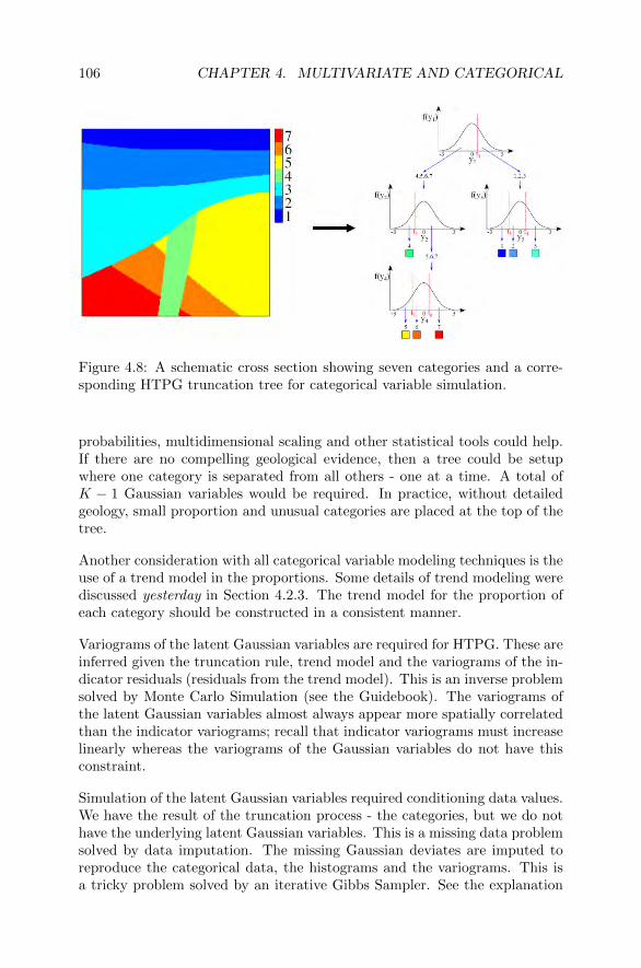
106 CHAPTER 4. MULTIVARIATE AND CATEGORICAL
Figure 4.8: A schematic cross section showing seven categories and a corre-sponding HTPG truncation tree for categorical variable simulation.
probabilities, multidimensional scaling and other statistical tools could help.If there are no compelling geological evidence, then a tree could be setupwhere one category is separated from all others - one at a time. A total ofK − 1 Gaussian variables would be required. In practice, without detailedgeology, small proportion and unusual categories are placed at the top of thetree.
Another consideration with all categorical variable modeling techniques is theuse of a trend model in the proportions. Some details of trend modeling werediscussed yesterday in Section 4.2.3. The trend model for the proportion ofeach category should be constructed in a consistent manner.
Variograms of the latent Gaussian variables are required for HTPG. These areinferred given the truncation rule, trend model and the variograms of the in-dicator residuals (residuals from the trend model). This is an inverse problemsolved by Monte Carlo Simulation (see the Guidebook). The variograms ofthe latent Gaussian variables almost always appear more spatially correlatedthan the indicator variograms; recall that indicator variograms must increaselinearly whereas the variograms of the Gaussian variables do not have thisconstraint.
Simulation of the latent Gaussian variables required conditioning data values.We have the result of the truncation process - the categories, but we do nothave the underlying latent Gaussian variables. This is a missing data problemsolved by data imputation. The missing Gaussian deviates are imputed toreproduce the categorical data, the histograms and the variograms. This isa tricky problem solved by an iterative Gibbs Sampler. See the explanation

4.4. SETUP AND POST PROCESSING 107
and software covered in the Guidebook.
The remaining practical steps of HTPG are quite straightforward. The sim-ulation of the latent variables is accomplished with SGS or with an uncondi-tional algorithm followed by conditioning. The simulated Gaussian values aretruncated and categorical variable realizations are constructed. They mustbe checked and validated to the greatest extent possible. A k-fold valida-tion scheme should be implemented and the accuracy and precision of thepredictions should be checked.
4.3.4 Exercise W4-3
This exercise will introduce some categorical variable modeling techniquesusing a large indicator data set. Indicator kriging and sequential indicatorsimulation will be used. Consider the indicator variable in sic.dat.
1. Plot a location map of the data and run cell declustering with a reason-able cell size: 15000 m is likely reasonable. What are the declusteredproportions? What is the declustered variance?
2. Calculate and model directional indicator variograms. As there are only2 categories (0 and 1), the variograms for each category will be identical.Pick a reasonable azimuth for the major direction based on the locationmap.
3. Use indicator kriging with the declustered proportions and modeledvariograms to estimate proportions over the domain and plot the results.Do they match the data?
4. Create 100 realizations of the domain using sequential indicator simu-lation. Post-process the realizations to calculate the e-type mean andentropy. Plot the first 2 realizations, the e-type mean and entropy.Comment on your results and compare the e-type mean with the indi-cator kriging maps.
4.4 Setup and Post Processing
4.4.1 Indicator Kriging and Uniform Conditioning
Multiple indicator kriging (MIK) has the promise of estimating local condi-tional distributions of uncertainty without a strong dependence on the mul-tivariate Gaussian distribution [35]. The Lesson on MIK is a nice summary[8].

108 CHAPTER 4. MULTIVARIATE AND CATEGORICAL
1. Choosing thresholds is the first step of MIK. The number of thresholdsis normally chosen between 7 to 15; considering too many may inducemore order relation problems and too few thresholds would result inlow resolution of the predicted distributions. Some criteria for choosingthe thresholds include: (1) commonly start with nine thresholds definingdeciles of the global distribution, (2) Move the thresholds to correspondto interesting inflection points on the cumulative distribution function,(3) Remove some low thresholds depending on the cutoff grade and addsome high thresholds to define approximately equal quantity of metal inthe upper classes, (4) Move the thresholds so one matches the specifiedcutoff grade, and (5) Intervals should have enough data for a robustestimation; perhaps a minimum of 5% of the data.
2. Indicator variograms are required for every threshold. These variogramsare often well behaved as the data are only 0s and 1s. Nevertheless,carefully choosing orientations and variogram parameters is still nec-essary to acquire stable variograms. The indicator variograms shouldbe standardized to make it easier to analyze, compare and model theindicator variograms. Any licit variogram structure that rises linearlyat the origin such as exponential and spherical can be used for modelingthe variograms. It is convenient to use the same type for all indicatorvariograms to ensure consistent changes. The indicator variograms, af-ter all, relate to the same underlying continuous variable. Transitionsbetween the indicator variograms are expected to be smooth in termsof variance, anisotropy, and ranges. To check these transitions fromone indicator to the next, the ranges, nugget effects and anisotropy canbe plotted versus the threshold number. There should be no abruptdiscontinuity between variograms of consecutive thresholds.
3. Indicator kriging (perhaps Markov-Bayes), order relations correction4. Post processing
Uniform conditioning is another technique to predict the uncertainty in SMUgrades given local panel estimate conditions.
1. Consider four scales (see Figure 4.9)2. Basic data scale statistics3. Ordinary kriging at the panel scale4. Calculate the distribution of SMU grades within each panel
Localization will be mentioned here.
1. Distribution of SMU grades within each panel - could come from UC,MIK, MG or simulation
2. Choose SMU grades - as many as there are SMUs within the panel3. Assign values based on a localizing variable

4.4. SETUP AND POST PROCESSING 109
Figure 4.9: Illustration of the four scales involved in uniform conditioning:the data, the SMU, panel and domain.
4.4.2 Post Processing
Setup of model - parameter uncertainty, data uncertainty, simulate realiza-tions, process through a transfer function, report uncertainty and sensitivity.
Local uncertainty, block averaging (upscaling), data spacing (Lesson [49]) andlocalization
Take expected value as late as possible. Calculate on all realizations, thentake the average as late as possible.
Grade control - calculate profit for all possibilities and all realizations, thentake the decision that maximizes the expected profit. The resolution of theprediction should be at a resolution of one quarter of the data spacing toprovide the best possible boundary.
4.4.3 Model Setup
Post processing is straightforward with estimation or deterministic models.Categories representing the geology is modeled first, then the grades are mod-eled within categories. The estimates are clipped by maximum drill hole spac-ing and the results are validated and checked to the greatest extent possible.Post processing simulated realizations is more challenging given the multiplemodels.
A high resolution data spacing model is important to clip estimates/simulatedvalues and to understand how uncertainty depends on data spacing. In 2-D

110 CHAPTER 4. MULTIVARIATE AND CATEGORICAL
a constant n approach is used - the area within:
dhs =
√πr2
n
where r is the radius half way between the distance that includes n and n+1.Often, a value of n between 10 to 20 is considered. In cases of irregular 3-D spacing of data, a constant volume approach is often considered. A largevolume oriented with the overall anisotropy is considered, the number of datawithin that volume are counted, the equivalent square spacing relative to theplane of continuity is computed by calibration.
Setup a modern simulation study for a variety of objectives
Loop back to the cover image
Parameter uncertainty with the multivariate spatial bootstrap [60].
Simulated realizations are often scaled up to nominal production volumesof months, quarters or years. Then, the uncertainty is calibrated to thedrill hole spacing. Uncertainty is often summarized as the probability to bewithin 15% of predicted (P ∈ ±15). Uncertainty is not simply related to thedata spacing. Other modifying factors include (1) the geological complexity -perhaps summarized by H, (2) the proportional effect, (3) the distance to theclosest drill hole, and other factors. A response surface model (RSM) couldbe built to quantify how each factor is contributing.
The drill hole spacing and uncertainty response curve is considered carefullyto understand when there is little response and when uncertainty is respond-ing quickly to more data. Figure 4.10 shows the learning curve concept ofhow uncertainty responds to more data.
Classification decisions must always depend on the qualified or competentperson. Uncertainty such a ”quarterly production volumes must be within15% of predicted 90% of the time or more.” Sometimes drill holes have to beremoved to understand uncertainty at a larger spacing. Sometimes we mustdrill a simulated realization to understand how uncertainty responds to drillhole spacings that have not been seen.
4.4.4 Exercise W4-4
The objectives of this exercise are to learn how to post process a set of multiplerealizations. Data spacing, localization and other topics will be summarized.
1. Consider the multiple realizations of Au for the Misima data (earlier
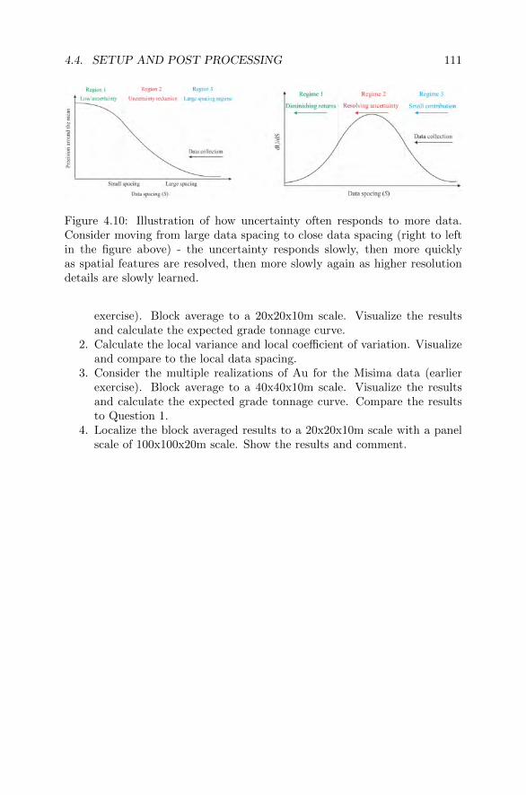
4.4. SETUP AND POST PROCESSING 111
Figure 4.10: Illustration of how uncertainty often responds to more data.Consider moving from large data spacing to close data spacing (right to leftin the figure above) - the uncertainty responds slowly, then more quicklyas spatial features are resolved, then more slowly again as higher resolutiondetails are slowly learned.
exercise). Block average to a 20x20x10m scale. Visualize the resultsand calculate the expected grade tonnage curve.
2. Calculate the local variance and local coefficient of variation. Visualizeand compare to the local data spacing.
3. Consider the multiple realizations of Au for the Misima data (earlierexercise). Block average to a 40x40x10m scale. Visualize the resultsand calculate the expected grade tonnage curve. Compare the resultsto Question 1.
4. Localize the block averaged results to a 20x20x10m scale with a panelscale of 100x100x20m scale. Show the results and comment.

112 CHAPTER 4. MULTIVARIATE AND CATEGORICAL

Appendix A
Additional Information
Software Setup
Any software could be used. There are commercial software that performsthe requested calculations. The GSLIB software, updated versions and addi-tional software from the Centre for Computational Geostatistics (CCG) areprovided for all participants in the Citation program. The preferred approachto run all computer exercises (all but three) is to run the entire exercise in aJupyter notebook, then export the notebook as an html file and submit thatas the solution. There are many online resources for this and the wealth ofinformation online cannot be repeated here. Some tips are provided.
The first step to getting setup for running the Citation exercises is to en-sure that you have a clean installation of Anaconda. Depending on yourcomfort with this platform, you may have to remove old versions or setupa new environment. You will also have to have a version of GIT installedon your computer (https://git-scm.com/) since this is used by pygeostatto access the executables. If necessary, you could copy the executables tothe correct location and avoid the use of git. You should bookmark (http://www.ccgalberta.com/pygeostat/welcome.html) which is the pygeostat doc-umentation since this will be referred to extensively.
Many notebooks that illustrate different calculations are provided with thecourse material. These should be reviewed. There are many ways to launcha notebook. The simplest way is to open the Anaconda Prompt and installpygeostat: pip install pygeostat. The small batch file CitNotebook.bat couldbe copied to your installation directory (C:/Users/Clayton/anaconda3 on mycomputer) and edit appropriately. This is to open a jupyter notebook in the
113

114 APPENDIX A. ADDITIONAL INFORMATION
right place.
An important step in the Citation is to review the introduction and learningnotebooks that have been provided: Py1Basics.ipynb, Py2GSLIB.ipynb andPy3Pygeostat.ipynb. For those that still use legacy GSLIB code for certainplotting functions - review the notebook and example in the Postscript
directory.
Support
There is none. Questions can be sent to the instructor of the class andany designated teaching assistants; however, everyone will have to strugglethrough learning how to bend the computer to your will.
Plots and Colors
The color scales and choices available at (https://colorbrewer2.org) should beconsidered. Colors should also be standardized across a project and, perhaps,an entire organization looking the same commodity.
Bibliography
[1] A. S. Almeida and A. G. Journel. Joint simulation of multiple vari-ables with a Markov-type coregionalization model. Mathematical Geol-ogy, 26:565–588, 1994.
[2] O. Babak and C. V. Deutsch. An intrinsic model of coregionalizationthat solves variance inflation in collocated cokriging. Computers & Geo-sciences, 2007.
[3] J. Bai and C. V. Deutsch. The pairwise relative variogram. InJ. L. Deutsch, editor, Geostatistics Lessons. 2020. Retrieved fromhttp://www.geostatisticslessons.com/lessons/pairwiserelative.
[4] R. M. Barnett. Principal component analysis. In J. L.Deutsch, editor, Geostatistics Lessons. 2017. Retrieved fromhttp://www.geostatisticslessons.com/lessons/principalcomponentanalysis.html.
[5] R. M. Barnett. Projection pursuit multivariate transform. InJ. L. Deutsch, editor, Geostatistics Lessons. 2017. Retrieved fromhttp://www.geostatisticslessons.com/lessons/lineardecorrelation.html.
[6] R. M. Barnett. Sphereing and min/max autocorrelation factors. InJ. L. Deutsch, editor, Geostatistics Lessons. 2017. Retrieved fromhttp://www.geostatisticslessons.com/lessons/errorellipses.
[7] F. A. Camana and C. V. Deutsch. The nugget effect. InJ. L. Deutsch, editor, Geostatistics Lessons. 2019. Retrieved fromhttp://www.geostatisticslessons.com/lessons/nuggeteffect.
[8] D. Carvalho and C. V. Deutsch. An overview of multiple indicator krig-ing. In J. L. Deutsch, editor, Geostatistics Lessons. 2017. Retrieved fromhttp://www.geostatisticslessons.com/lessons/mik.
[9] J. P. Chiles and P. Delfiner. Geostatistics: modeling Spatial Uncertainty.Wiley Series in Probability and Statistics, 2nd edition, April 2012.
115

116 BIBLIOGRAPHY
[10] A. P. Chiquini and C. V. Deutsch. A simulation ap-proach to calibrate outlier capping. In J. L. Deutsch,editor, Geostatistics Lessons. 2017. Retrieved fromhttp://www.geostatisticslessons.com/lessons/simulationcapping.
[11] M. David. Geostatistical Ore Reserve Estimation. Elsevier, Amsterdam,1977.
[12] C. Deutsch. Calculating effective absolute permeability in sand-stone/shale sequences. SPE Formation Evaluation, pages 343–348,September 1989.
[13] C. Deutsch and A. Journel. GSLIB: Geostatistical Software Library andUser’s Guide. Oxford University Press, New York, 2nd edition, 1995. InPress.
[14] C. V. Deutsch. Kriging in a finite domain. Mathematical Geology,25(1):41–52, 1993.
[15] C. V. Deutsch. Direct assessment of local accuracy and precision. InE. Y. Baafi and N. A. Schofield, editors, Fifth International GeostatisticsCongress, pages 115–125, Wollongong, Australia, Sept. 1996.
[16] C. V. Deutsch. Cleaning categorical variable (lithofacies) realiza-tions with maximum a-posteriori selection. Computers & Geosciences,24(6):551–562, 1998.
[17] C. V. Deutsch. A sequential indicator simulation program for categori-cal variables with point and block data: BlockSIS. Computers & Geo-sciences, 32(10):1669–1681, 2006.
[18] C. V. Deutsch. Cell declustering parameter selection. In J. L.Deutsch, editor, Geostatistics Lessons. 2015. Retrieved fromhttp://www.geostatisticslessons.com/lessons/celldeclustering.
[19] C. V. Deutsch. Checking simulated realizations - mining. InJ. L. Deutsch, editor, Geostatistics Lessons. 2017. Retrieved fromhttp://www.geostatisticslessons.com/lessons/checkingmin.
[20] C. V. Deutsch and J. L. Deutsch. Introduction to choosing a krigingplan. In J. L. Deutsch, editor, Geostatistics Lessons. 2015. Retrievedfrom http://www.geostatisticslessons.com/lessons/introkrigingplan.
[21] C. V. Deutsch and J. L. Deutsch. An applicationof Bayes theorem to geostatistical mapping. In J. L.Deutsch, editor, Geostatistics Lessons. 2018. Retrieved fromhttp://www.geostatisticslessons.com/lessons/bayesmapping.

BIBLIOGRAPHY 117
[22] C. V. Deutsch and P. Kumara. Transforming a var-iogram of normal scores to original units. In J. L.Deutsch, editor, Geostatistics Lessons. 2017. Retrieved fromhttp://www.geostatisticslessons.com/lessons/convertnsvariograms.
[23] J. Deutsch, J. Szymanski, and C. Deutsch. Checks and measures ofperformance for kriging estimates. The Journal of the Southern AfricanInstitute of Mining and Metallurgy (SAIMM), 114:223–230, Mar. 2014.
[24] J. L. Deutsch. Experimental variogram tolerance parameters. InJ. L. Deutsch, editor, Geostatistics Lessons. 2015. Retrieved fromhttp://www.geostatisticslessons.com/lessons/variogramparameters.
[25] J. L. Deutsch. Variogram calculation for tabular deposits. InJ. L. Deutsch, editor, Geostatistics Lessons. 2015. Retrieved fromhttp://www.geostatisticslessons.com/lessons/tabularvariograms.
[26] M. V. Deutsch. The angle specification for gslib software. InJ. L. Deutsch, editor, Geostatistics Lessons. 2015. Retrieved fromhttp://www.geostatisticslessons.com/lessons/errorellipses.
[27] O. Erten and C. V. Deutsch. Combination of multivari-ate gaussian distributions through error ellipses. In J. L.Deutsch, editor, Geostatistics Lessons. 2020. Retrieved fromhttp://www.geostatisticslessons.com/lessons/errorellipses.
[28] P. Goovaerts. Geostatistics for Natural Resources Evaluation. OxfordUniversity Press, New York, 1997. In Press.
[29] E. Gringarten and C. V. Deutsch. Methodology for variogram interpre-tation and modeling for improved petroleum reservoir characterization.In 1999 SPE Annual Technical Conference and Exhibition FormationEvaluation and Reservoir Geology, Houston, TX, Oct. 1999. Society ofPetroleum Engineers. SPE Paper # 56654.
[30] J. Hammersley and D. Handscomb. Monte Carlo Methods. John Wiley& Sons, New York, 1964.
[31] B. E. Harding and C. V. Deutsch. Change of sup-port and the volume variance relation. In J. L. Deutsch,editor, Geostatistics Lessons. 2019. Retrieved fromhttp://www.geostatisticslessons.com/lessons/changeofsupport.
[32] H. Hotelling. Analysis of a complex of statistical variables into principalcomponents. Journal of Educational Psychology, 24:417–441, 1933.
[33] E. Isaaks and R. Srivastava. Spatial continuity measures for probabilisticand deterministic geostatistics. Math Geology, 20(4):313–41, 1988.
118 BIBLIOGRAPHY
[34] E. Isaaks and R. Srivastava. An Introduction to Applied Geostatistics.Oxford University Press, New York, 1989.
[35] A. Journel. Non-parametric estimation of spatial distributions. MathGeology, 15(3):445–68, 1983.
[36] A. Journel. Fundamentals of Geostatistics in Five Lessons. Volume8 Short Course in Geology. American Geophysical Union, Washington,D.C., 1989.
[37] A. Journel and C. J. Huijbregts. Mining Geostatistics. Academic Press,New York, 1978.
[38] A. G. Journel. Markov models for cross-covariances. Mathematical Ge-ology, 31(8):955–964, 1999.
[39] A. G. Journel. Combining knowledge from diverse sources: an alterna-tive to traditional data independence hypotheses. Mathematical Geology,34(5), 2002.
[40] D. G. Krige. A statistical approach to some mine valuations and alliedproblems at the witwatersrand. Master’s thesis, University of Witwater-srand, South Africa, 1951.
[41] O. Leuangthong and C. V. Deutsch. Stepwise conditional transformationfor simulation of multiple variables. Mathematical geology, 35(2):155–173,2003.
[42] D. Luenberger. Optimization by Vector Space Methods. John Wiley &Sons, New York, 1969.
[43] S. A. Mancell and C. V. Deutsch. Multidimensional scaling. InJ. L. Deutsch, editor, Geostatistics Lessons. 2019. Retrieved fromhttp://www.geostatisticslessons.com/lessons/mds.
[44] G. Matheron. Traite de geostatistique appliquee. Vol. 1 (1962), Vol. 2(1963), ed. Technip, Paris, 1962.
[45] H. Parker. The volume-variance relationship: a useful tool for mineplanning. In P. Mousset-Jones, editor, Geostatistics, pages 61–91, NewYork, 1980. McGraw Hill.
[46] H. Parker. Statistical treatment of outlier data in epithermal gold depositreserve estimation. Math Geology, 23(2):175–199, 1991.
[47] K. Pearson. On lines and planes of closest fit to systems of points inspace. Philosophical Magazine, 2(11):559–572, 1901.
[48] F. L. Pereira and C. V. Deutsch. Permanence of ratios. InJ. L. Deutsch, editor, Geostatistics Lessons. 2020. Retrieved fromhttp://www.geostatisticslessons.com/lessons/permanenceofratios.
BIBLIOGRAPHY 119
[49] F. A. C. Pinto and C. V. Deutsch. Calculation of high resolution dataspacing models. In J. L. Deutsch, editor, Geostatistics Lessons. 2017. Re-trieved from http://www.geostatisticslessons.com/lessons/dataspacing.
[50] M. Pyrcz and C. Deutsch. Geostatistical Reservoir Modeling. OxfordUniversity Press, New York, 2nd edition, 2014.
[51] M. J. Pyrcz and C. V. Deutsch. Transforming data to a gaussian distri-bution. In J. L. Deutsch, editor, Geostatistics Lessons. 2018. Retrievedfrom http://www.geostatisticslessons.com/lessons/normalscore.
[52] M. Samson and C. V. Deutsch. Collocated cokriging. InJ. L. Deutsch, editor, Geostatistics Lessons. 2020. Retrieved fromhttp://www.geostatisticslessons.com/lessons/collocatedcokriging.
[53] L. E. Shmaryan and A. G. Journel. Two Markov models and their ap-plication. Mathematical Geology, 31(8):965–988, 1999.
[54] D. A. Silva. Signed distance function modeling with multiple categories.In J. L. Deutsch, editor, Geostatistics Lessons. 2015. Retrieved fromhttp://www.geostatisticslessons.com/lessons/signeddistancefunctions.
[55] R. Srivastava and H. Parker. Robust measures of spatial continuity. InM. Armstrong, editor, Geostatistics, pages 295–308. Reidel, Dordrecht,Holland, 1988.
[56] C. A. Sunday and C. V. Deutsch. Choosing the dis-cretization level for block property estimation. In J. L.Deutsch, editor, Geostatistics Lessons. 2020. Retrieved fromhttp://www.geostatisticslessons.com/lessons/discretization.
[57] P. Switzer. Inference for spatial autocorrelation functions. In G. Verlyet al., editors, Geostatistics for Natural Resources Characterization, vol-ume 1, pages 127–140. Reidel, Dordrecht, Holland, 1984.
[58] J. Tukey. Exploratory Data Analysis. Addison-Wesley, Reading, MA,1977.
[59] G. Verly. The multiGaussian approach and its applications to the esti-mation of local reserves. Math Geology, 15(2):259–86, 1983.
[60] J. D. Vincent and C. V. Deutsch. The multivariate spatial bootstrap.In J. L. Deutsch, editor, Geostatistics Lessons. 2019. Retrieved fromhttp://www.geostatisticslessons.com/lessons/spatialbootstrap.
[61] H. Wackernagel. Multivariate Geostatistics: An Introduction with Appli-cations. Springer-Verlag, Berlin, 1995.

120 BIBLIOGRAPHY
[62] D. Yang and C. V. Deutsch. Aggregating multiple sec-ondary variables into a super secondary variable. In J. L.Deutsch, editor, Geostatistics Lessons. 2019. Retrieved fromhttp://www.geostatisticslessons.com/lessons/supersecondary.
[63] H. Zhang, O. Erten, and C. V. Deutsch. Bayesian up-dating for combining conditional distributions. In J. L.Deutsch, editor, Geostatistics Lessons. 2020. Retrieved fromhttp://www.geostatisticslessons.com/lessons/bayesianupdating.


![Chapter 1 Geostatistics in Hydrology: Kriging interpolationberga/Teaching/STAM/stat.pdf · Geostatistics in Hydrology: Kriging interpolation ... [4, 5] and largely applied in](https://img.dokumen.tips/doc/110x75/5abeb8417f8b9aa15e8d2ce2/chapter-1-geostatistics-in-hydrology-kriging-bergateachingstamstatpdfgeostatistics.jpg)