Embed Size (px)
Citation preview

Fall 2019
Project 1: Face Recognition
CIS4930 / CIS6930 Biometric
Authentication on Mobile Devices
University of South Florida
Department of Computer Science and Engineering
Instructor: Dr. Tempestt Neal

Project 1 Group #1
Introduction A. Understanding Biometrics
The study of biometrics has been an ongoing topic that continues to expand as the importance of more secure applications are discussed. From government offices to simply identifying oneself as a citizen, biometric recognition is critical in many applications to ensure a secure biometric system. Biometrics is the science of setting up the identity of an individual based on physical characteristics, behavioral characteristics, or both of that person either in a fully automated or semi-automated manner. When considering the aspects of biometric recognition, there are knowledge-based, or token-based attributes to authenticating a user. Each of these has their own positives and negatives, but they are the basis for determining how a user is to be authenticated by a biometric system. Biometric recognition is important for ensuring a reliable and natural solution to recognizing a person in a system. The person who presents their biometric identifier to a biometric system to be recognized is called a user of the system. The user must be present at the time of the authentication, which also helps to prevent imposters from accessing the system. Biometrics can also establish whether a user is already known within the system or not. The biometric system itself measures one or more physical or behavioral characteristics, such as face, fingerprint, iris, voice, signature, gait, palmprint, retina, or DNA. Each of these pieces of information can be used to verify someone’s identity. B. The Biometric System
The biometric system exists to identify a user based on the physical characteristics, behavioral characteristics, or both. There
are two main phases in the process of the system, enrollment and recognition. In the enrollment phase, biometric data from the user seeking to enroll themselves in the system is obtained and stored within a database along with their identity. During the recognition phase, the user becomes the query instead of simply enrolling. To authenticate themselves with the system, biometric data is re-acquired from the individual and compared against the data stored in the database to determine the user’s identity. This part is referred to as matching. The decision determined from the matching process will inform the user if they are authenticated with the system or not. In general, the biometric systems consists or a sensor, feature extractor, database, and a matcher. C. Face Recognition
Face is the most commonly used biometric traits used in the biometric research area. A human face exposes a great deal of information for perceivers. An individual’s mood, attentiveness, and intention are seen at face, and it also serves to identify the person. There are additional means to identify a person than face. For instance, gait, body shape, and voice may all help in identifying persons when facial information is not available.
Face recognition involves the matching between the structural coding and previously stored data. The face recognition helps in deciding whether the initial matching is sufficient and close to accurate recognition, or it is merely a resemblance. Among research topics, face recognition is one of the active topics in the area of computer vision. It is because various face recognition techniques perform well in a
Fall 2019: Biometric Authentication on Mobile Devices 1

controlled environment. However, these techniques suffer when variation is observed among factors such as illumination and pose. Therefore, research is on the way to increase the robustness of face recognition techniques by eliminating the effects of influencing factors.
Face recognition starts matching between detected face and face ID stored in a database. Between detected face and stored information, an algorithm works that converts face features into machine readable format.
Once the face is recognized, facial recognition algorithm executes to identify the certain points of the face i.e. spot between pupils. Then the algorithm uses the measured points and creates a template or pattern of a face. Then the newly created template or pattern is compared with others already stored in the database.
Principal component analysis (PCA) is one of these techniques that computes the reduced set of factors. The PCA technique serves as a linear transformation from the space of the original image. Furthermore, local binary patterns (LBP) is a crucial performing technique in the area of face recognition. Since a face is composed of micro-patterns and LBP is the most appropriate to analyze them. In combination with LBP, PCA is applied to reduce the size of the vector. From a large set of variables, PCA extracts the most important variables to examine the information exactly.
In comparison with the other popular biometric techniques, including iris, retina, and fingerprint recognition, face recognition has the potential to be used in surveillance security, digital entertainment, and forensics.
Methods
There are various matching methods for fingerprint authentication, all of which rely on some kind of algorithm for matching minutiae. The following are just a few:
K Nearest Neighbors, a classification algorithm that utilizes other ‘close’ examples in the data set (neighbors) to assign a classifier. The number, k, must be odd in order to prevent ties.
● Benefits: it’s simple and easy to implement. Allows for system updating with each new query (can add to the example pool with each correct classification). The more it is used, the better it becomes with classifying.
● Cost: Choosing a value of k that is too large or too small may result in inaccurate results due to the search exceeding the limitations of the example pool (too many neighbors selected in the given neighborhood). Could also be vulnerable to overfitting/underfitting.
There are other variations of the K Nearest
Neighbors algorithm, such as the Condensed Nearest Neighbors algorithm. The CNN or Hart algorithm uses prototyping to condense and reduce the data set which helps with vulnerabilities to over/underfitting.
Normalized Cross Correlation (NCC) is a method that breaks a finger print down into smaller mosaic images of partial prints. It enhances the images with a thinning algorithm, before running a Phase-Only Correlation (POC) to find rotational and transformative differences between query and template. The query image is then superimposed over the template for comparison.
Fall 2019: Biometric Authentication on Mobile Devices 2

The purpose of a biometric matcher is to
contrast the query features against the templates in order to generate matching scores. A matching score measures the similarity between a query and a stored template. The greater similarities between the query and template are, the higher a matching score is. A matcher can also measure the dissimilarity between features. This measurement is referred to as the distance score. Thus, if a score shows a small distance score, this indicates that two features have a high matching score.
The matcher module encapsulates a decision making module, were the match scores are used to authenticate a claimed identity or provide a ranking of the enrolled identities in order to identify an individual. The fingerprint matcher performs template matching in a one-to-one comparison between a query and a claimed template, of a one-to-many comparisons between a query and all templates. The processes are used for the verification and identification of an individual.
Naive Bayes methods are a set of supervised and effective machine learning algorithms. It is a probability classifier that is based on the Bayes theorem where the probability of an event is measured by previous knowledge about items, elements, or characteristics that may lead to that event. System Architectures
There are two system architectures used in this face recognition system which are brightness image enhancement and contrast image enhancement.
The most important factor for a face recognition system to recognize, verify or identify a person easily is using images that have a proper level of brightness and
contrast. According to Olympus, contrast is the amount of color of grayscale differentiation that exists between various image features in both analog and digital images [2]. Images having a higher contrast level generally display a greater degree of color or grayscale variation than those of lower contrast. Image brightness (or luminous brightness) is a measure of intensity after the image has been acquired with a digital camera or digitized by an analog-to-digital converter [2].
In the given data set, there are images that were taken in the dark. Therefore, we used the image enhancement library PIL (short for Pillow (PIL Fork)). Out of four image enhancement classes (Sharpness, Color, Brightness and Contrast). Our team chose to enhance the brightness and contrast of the images to compare the performances of each of the enhancements to the original images. For both enhancement classes, they use a single common method containing enhance(factor) and it returns an enhanced image. The contrast class is used to adjust the level of contrast of an image. A factor of 0.0 gives a solid grey image. A factor of 1.0 gives the original image. Similarly, the brightness class can also be used to adjust the overall brightness for an image. A factor of 0.0 gives a black image. A factor of 1.0 also gives the original image [3]. In our image enhancement implementation (enhance_images.py), the brightness factor
is set 2.0. Figure 1 showed that the brightness was doubled in the comparison between the before and after images. Furthermore, the contrast factor is set to 0.5, it was reduced by half resulted in a blurry after image compares to the original photo, as shown in Figure 2.
The database we used for this project contains 5 main subjects. There are 114 images for subject 1, 97 images for subject 2, 98 images for subject 3, 92 images for
Fall 2019: Biometric Authentication on Mobile Devices 3

subject 4 and 99 for subject 5. They were generated from tasks our team performed.
The process of enhancing the images: First step is to set different cases for each of the enhancement classes for performance comparison purposes, such as case 1 is for the brightness enhancement and case 2 is for contrasting the images. Secondly, the code will go through each of the data folder (each team member’s face data which totals 500 images among all the folders); it will also run the PIL library to enhance the images based on the case selection and then make a new folder for each of the enhancement class for each of the team member such as Group1_FaceData_EnhancedBrightness and Group1_FaceData_EnhancedContrast.
The goal is to compare the performance of enhanced images to the performance of original images. In addition, analyze how enhancing the images can improve the results of the original images from the performed tasks.
Figure 1: Comparison of images before and after brightness enhancement.
Figure 2: Comparison of images before and after contrast enhancement.
Results
The results were determined by first identifying the performance of the original images by extracting their features with either local binary pattern (LBP) or principal component analysis (PCA). Once the features were obtained, a matcher was used to get all the genuine and imposter scores. These scores were used to generate the score distributions, ROC curves, and DET curves.
To define the architectures used, the original images were compared with enhanced versions of those images to record any differences in performance that existed between the score distributions, ROC curves, and DET curves for both PCA and LBP, as well as with the KNN and Naive Bayes (NB) matchers. The two primary additional architectures were to brighten the images and add sharpness to the images. The KNN matcher was classified with 50 neighbors and manhattan distance as the metric. A. Original Results
The original images were tested by first storing the images and their labels into two numpy arrays. The images were passed through either LBP and PCA to get the features of the images. Next, a matcher for KNN or Naive Bayes was used to determine the number of genuine and imposter scores. Afterwards, the performance results could be determined on the score distribution, ROC curve, and DET curve. The results will be numbered from (1 - 4), indicating the test performed to be used for comparison with the enhanced images. 1. When running LBP with the KNN matcher on the images the following figures show the results.
Fall 2019: Biometric Authentication on Mobile Devices 4
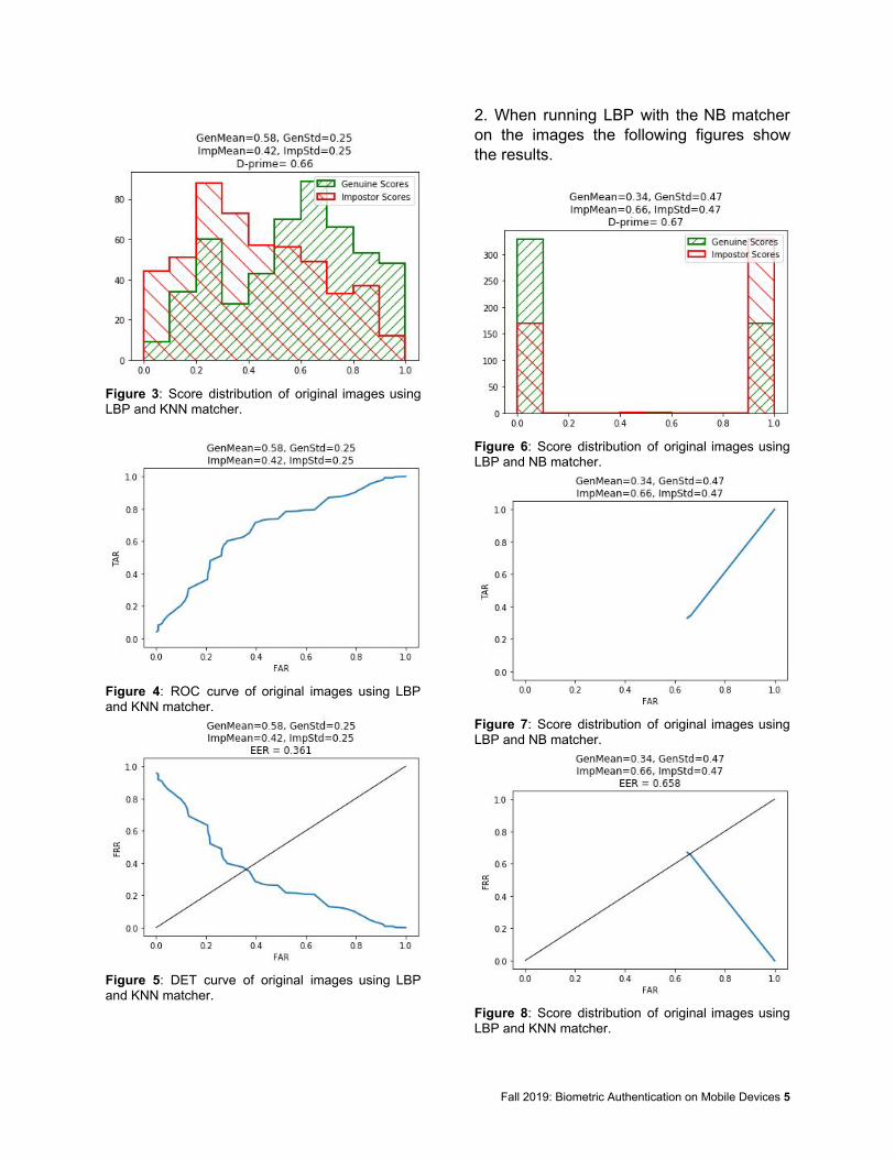
Figure 3: Score distribution of original images using LBP and KNN matcher.
Figure 4: ROC curve of original images using LBP and KNN matcher.
Figure 5: DET curve of original images using LBP and KNN matcher.
2. When running LBP with the NB matcher on the images the following figures show the results.
Figure 6: Score distribution of original images using LBP and NB matcher.
Figure 7: Score distribution of original images using LBP and NB matcher.
Figure 8: Score distribution of original images using LBP and KNN matcher.
Fall 2019: Biometric Authentication on Mobile Devices 5

3. When running PCA with the KNN matcher on the images the following figures show the results.
Figure 9: Score distribution of original images using PCA and KNN matcher.
Figure 10: ROC curve of original images using PCA and KNN matcher.
Figure 11: DET curve of original images using PCA and KNN matcher.
4. When running PCA with the NB matcher on the images the following figures show the results.
Figure 12: Score distribution of original images using PCA and NB matcher.
Figure 13: ROC curve of original images using PCA and NB matcher.
Figure 14: DET curve of original images using PCA and NB matcher.
Fall 2019: Biometric Authentication on Mobile Devices 6

Now, the comparison will be drawn with
the two additional architectures, both being a form of image enhancement. B. Architecture 1 - Brightness Enhancement
The first image enhancement was brightening the images by doubling the brightness value on the image. It is possible to do this, because images can be enhanced with Python PIL [1]. 1. When running LBP with the KNN matcher on the images the following figures show the results.
Figure 15: Score distribution of brightened images using LBP and KNN matcher.
Figure 16: ROC curve of brightened images using LBP and KNN matcher.
Figure 17: DET curve of brightened images using LBP and KNN matcher. 2. When running LBP with the NB matcher on the images the following figures show the results.
Figure 18: Score distribution curve of brightened images using LBP and NB matcher.
Figure 19: ROC curve of brightened images using LBP and NB matcher.
Fall 2019: Biometric Authentication on Mobile Devices 7

Figure 20: DET curve of brightened images using LBP and NB matcher. 3. When running PCA with the KNN matcher on the images the following figures show the results.
Figure 21: Score distribution of brightened images using PCA and KNN matcher.
Figure 22: ROC curve of brightened images using PCA and KNN matcher.
Figure 23: DET curve of brightened images using PCA and KNN matcher. 4. When running PCA with the NB matcher on the images the following figures show the results.
Figure 24: Score distribution of brightened images using PCA and NB matcher.
Fall 2019: Biometric Authentication on Mobile Devices 8

Figure 25: ROC curve of brightened images using PCA and NB matcher.
Figure 26: DET curve of brightened images using PCA and NB matcher.
Original Image Brightened Image
Test 1 (LBP w/ KNN)
d-prime = 0.660 EER = 0.361
d-prime = 0.830 EER = 0.340
Test 2 (LBP w/ NB)
d-prime = 0.670 EER = 0.658
d-prime = 0.330 EER = 0.580
Test 3 (PCA w/ KNN)
d-prime = 0.170 EER = 0.521
d-prime = 0.500 EER = 0.432
Test 4 d-prime = 0.050 d-prime = 0.590
(PCA w/ NB)
EER = 0.486 EER = 0.730
Table 1: Performance results of brightened images versus original images.
Using the results from Table 1, for test 1, the original images obtained a d-prime value of 0.660 on the score distribution and an EER of 0.361, while the brightened images obtained a d-prime value of 0.830 and an EER of 0.340. This shows that for LBP with the KNN matcher, the brightened images had a better performance than the original images.
For test 2, the original images obtained a d-prime value of 0.670 on the score distribution and an EER of 0.658, while the brightened images obtained a d-prime value of 0.330 and an EER of 0.580. This shows that for LBP with the NB matcher, the original images had a better performance than the brightened images.
For test 3, the original images obtained a d-prime value of 0.170 on the score distribution and an EER of 0.521, while the brightened images obtained a d-prime value of 0.500 and an EER of 0.432. This shows that for PCA with the KNN matcher, the brightened images had a better performance than the original images.
For test 4, the original images obtained a d-prime value of 0.050 on the score distribution and an EER of 0.486, while the brightened images obtained a d-prime value of 0.59 and an EER of 0.730. This shows that for PCA with the NB matcher, the brightened images had a better performance than the original images.
Overall, by brightening the images, a better performance can be expected.
Fall 2019: Biometric Authentication on Mobile Devices 9

C. Architecture 2 - Contrast Enhancement
The second image enhancement was contrasting the images by reducing the contrast value by 0.5. 1. When running LBP with the KNN matcher on the images the following figures show the results.
Figure 27: Score distribution of contrasted images using LBP and KNN matcher.
Figure 28: ROC curve of contrasted images using LBP and KNN matcher.
Figure 29: DET curve of contrasted images using LBP and KNN matcher. 2. When running LBP with the NB matcher on the images the following figures show the results.
Figure 30: Score Distribution of contrasted images using LBP and NB matcher.
Figure 31: ROC curve of contrasted images using LBP and NB matcher.
Fall 2019: Biometric Authentication on Mobile Devices 10

Figure 32: DET curve of contrasted images using LBP and NB matcher. 3. When running PCA with the KNN matcher on the images the following figures show the results.
Figure 33: Score distribution of contrasted images using PCA and KNN matcher.
Figure 34: ROC curve of contrasted images using PCA and KNN matcher.
Figure 35: DET curve of contrasted images using PCA and KNN matcher. 4. When running PCA with the NB matcher on the images the following figures show the results.
Figure 36: Score distribution of contrasted images using PCA and NB matcher.
Fall 2019: Biometric Authentication on Mobile Devices 11

Figure 37: ROC curve of contrasted images using PCA and NB matcher.
Figure 38: DET curve of contrasted images using PCA and NB matcher.
Original Image Contrasted Image
Test 1 (LBP w/ KNN)
d-prime = 0.660 EER = 0.361
d-prime = 1.25 EER = 0.293
Test 2 (LBP w/ PCA)
d-prime = 0.670 EER = 0.658
d-prime = 0.440 EER = 0.607
Test 3 (PCA w/ KNN)
d-prime = 0.170 EER = 0.521
d-prime = 0.610 EER = 0.557
Test 4 (PCA w/ NB)
d-prime = 0.050 EER = 0.486
d-prime = 0.880 EER = 0.751
Table 2: Performance results of contrasted images versus original images.
Using the results from Table 2, for test 1, the original images obtained a d-prime value of 0.660 on the score distribution and an EER of 0.361, while the contrasted images obtained a d-prime value of 1.25 and an EER of 0.293. This shows that for LBP with the KNN matcher, the contrasted images had a better performance than the original images.
For test 2, the original images obtained a d-prime value of 0.670 on the score distribution and an EER of 0.658, while the contrasted images obtained a d-prime value of 0.440 and an EER of 0.607. This shows that for LBP with the NB matcher, the original images had a better performance than the contrasted images.
For test 3, the original images obtained a d-prime value of 0.170 on the score distribution and an EER of 0.521, while the contrasted images obtained a d-prime value of 0.610 and an EER of 0.557. This shows that for PCA with the KNN matcher, the contrasted images had a better performance than the original images.
For test 4, the original images obtained a d-prime value of 0.050 on the score distribution and an EER of 0.486, while the contrasted images obtained a d-prime value of 0.880 and an EER of 0.751. This shows that for PCA with the NB matcher, the contrasted images had a better performance than the original images.
The images that were hardest to classify were the images that had been processed as Failure to Capture (FTC). These images
Fall 2019: Biometric Authentication on Mobile Devices 12

had the greatest impact on the data in regards to performance. Conclusions
In conclusion, the study of Biometrics is the science of determining the identity of an individual based on physical characteristics, behavioral characteristics, or both. The biometric system exists to identify a user based on the physical characteristics, behavioral characteristics, or both. Within the biometric system, enrollment and recognition are two main phases in the process of the system.
Face recognition is a process that involves matching between the structural coding and previously stored data of the face presented to the biometric system. There are various methods by which facial extraction is performed to retrieve the features of the face. Acquiring these features can allow for generating the genuine and imposter scores from matching classifiers to generate performance metrics.
The two primary architectures used in the experimentation were brightening the original images and contrasting the original images. From the tests performed, we learned that each of these enhancements proved to have better performance than the original counterpart in terms of d-prime from the score distribution and the EER from the DET curve. One consistent result that was in favor of the original images were from test 2. Running LBP with the NB matcher on the images always had better performance with the original images than the enhanced ones. We also learned that it is important to plan a consistent strategy for testing each of these performance metrics. Being that each image can have its features extracted using LBP or PCA, then run through either the KNN or NB matcher, it was important to organize the code to ensure we recorded the desired results accurately. Moreover, we
learned that in terms of extracting features, LBP with either the KNN or NB matcher had a better performance than PCA with either the KNN or NB matchers.
As it relates to the system, it was easy to operate with the original images to get the images from the folders and extract the features using PCA and LBP. Furthermore, running the matchers and determining the performance were not difficult. However, it was hard for the system to enhance the images and then process them in the same manner as with the original images. With the performance being overall better, it took the system much longer to process the images to extract features and run the matchers to see their performance.
In the future, there are many modifications we would like to make to the system to see how they affect the performance of the system. We could determine the performance of specific tasks instead of using the entire set of images. It is likely that removing the FTC images will improve the performance in the score distributions, ROC curves, and DET curves. We would also be interested in expanding our image set with different facial images to determine how that will affect the performance of the system. Other tests we could attempt are sharpening the images to see the performance compared to the original images. Combining every enhancement into the images would provide unique understanding of the changes in performance, as well. There is also the idea of incorporating score fusion into the project by taking the mean of the genuine and imposter scores for both matchers to determine how that affects our performance results.
The limitations to the approach we decided to do, is that by using the entire image set, we could expect the results to be less
Fall 2019: Biometric Authentication on Mobile Devices 13

defined instead of using a specific task’s images. References [1] Petercour. (1970, July 15). Enhance
image with Python PIL. Retrieved from https://dev.to/petercour/enhance-image-with-python-pil-222e.
[2] Brightness and Contrast in Digital Images. (n.d.). Retrieved from http://olympus.magnet.fsu.edu/primer/java/olympusmicd/digitalimaging/contrast/index.html.
[3] ImageEnhanceModule¶. (n.d.).Retrieved from https://pillow.readthedocs.io/en/3.0.x/reference/ImageEnhance.html.
Fall 2019: Biometric Authentication on Mobile Devices 14

Facial Recognition Architecture Analysis Group 2: Annie Brey, Chris Keller, Justin Tran, Jennyfer Munoz
I.Introduction
Biometrics are the measurements and calculations related to a human body. More specifically, it is the measurement and calculation of the unique identifying features of an individual. In terms of biometric authentication, biometrics could be anything that can identify a person, for instance their password or their fingerprint. Biometric authentication is a system that will give/deny you access to a device based on your biometric properties. Biometric authentication is used in everyday life to improve security measures. Biometrics in this case could be relating to what someone knows, like a password, what someone has, like a token or ID card, or who someone is, like someone’s fingerprint. Any of these methods can be utilized to provide additional security. For instance, many companies have employee ID card scanners at the entrance to the building so those who are not employees can not gain access. This adds a layer of security so a company will not have intruders stealing information from inside the building. Some authentication systems can even use multiple authentication methods in one system, which adds additional security. Some systems combine two of the above methods for example, an employee would have to present their employee ID card to scan and use their fingerprint which needs to match the ID on file. This adds another layer to security because both of the biometrics would have to match the employee in order for them to gain access.
There are many different types of biometric modalities which classify a biometric system and there is not one modality that is the most accurate or the best for every implementation. Some common modalities include, facial recognition, fingerprint recognition, and voice recognition. Facial recognition is becoming very popular in recent years due to mobile devices having this feature built in. However, facial recognition is not perfect because sometimes family members could have a similar enough face to unlock one another’s phones. How facial recognition systems work is the developer has certain mathematical formulas and certain machine learning models so the computer knows what to do with the image, then the developer will train the model with data, in this case faces. The demographics of the data being used to train the authentication model could affect which types of people it will more likely authenticate correctly or incorrectly, this is why it is important to have a wide variety of demographics and features so the authentication system can be accurate for every type of person.
We have developed a biometric authentication system that uses facial recognition as the modality. We have a total of 522 pictures of faces and most of those are used to train the model and the rest are used to test the performance of the model. We have also developed a photo enhancement method to compare the differences between the performance in the enhanced versus unenhanced pictures. We are also going to be comparing two different feature extraction methods Principal Component Analysis (PCA) and Local Binary Pattern (LBP).

II. Methods A. Enhancement
By implementing a type of enhancement on images, or data then it can affect how the raw data is taken in and that can either improve or worsen the effect of the feature extractions. Types of enhancements can be like putting more contrast or brightening the image. For this facial recognition system, there is the implementation of a Min Max Scalar function – this is similar to histogram stretching. This function transforms the specified image, by changing the features to a scale based on given thresholds. For instance, you provide the new min and max pixel values and it will transform the image to have the values only be between those values while maintaining the spread of the values correct so the overall image does not change. In our method, we choose a specific threshold to determine whether or not this enhancement will be used on the particular image. If images were darker than the threshold then this enhancement will be added, and it will be able to brighten up the image. In this image below, it shows an example of the effect of the enhancement.
B. Principal Component Analysis Annie
The methods we compared for feature extraction were Principal Component Analysis (PCA) and Local Binary Pattern (LBP). The first step for PCA is to “squash” the data, which in this case are the faces. So the data is reduced down to a one dimensional array with lower dimensions compared to the full picture, therefore it is easier for manipulation and produces a better processing time. PCA only accepts greyscale, face-centered pictures, therefore the data we entered has to be normalized. The PCA function has a way to normalize the data. This includes finding the mean pixel value and subtracting that from each of the pixels, which will shift the data and center everyone’s face in the frame. With the normalized data PCA will then compute the covariance matrix by evaluating C = A’A, where C is the covariance matrix and A is the vector of faces. We compute A’A to save space compared to AA’. Next, PCA gets the eigenfaces from the covariance matrix and retains the top 20 eigenvectors corresponding with the highest 20 eigenvalues. The PCA method used the top 20 because in testing this performed better than other lower or higher values. This will extract and return the features of each face from the eigen faces. PCA takes a much shorter processing time compared to LBP because this method decreases the dimensions to save processing power and therefore saves time. C. Local Binary Patterns

This is a type of visual descriptor that can be utilized for feature extraction. This priorities texture in images, it analyzes the neighbor pixels in order to determine what the texture value is. The histogram of all the pixels make up the texture descriptor. This can be used with varying size of the neighbors, for this project it is used with 16 neighbors. This is important because sometimes images get affected by lighting. The way that this works is that it considers the pixels neighbors and compares the neighbor values to the pixel and then outputs the binary string, converted to decimal. Based on the values of the 8 -bin values, it forms a local histogram, and then the concatenation of the histogram is the features that can be used.
D. k-Nearest Neighbors Annie
The K-Nearest Neighbors (KNN) algorithm is the method we used for matching. Matching is how the system determines whether a query is genuine or an imposter. The matching algorithm compares how similar the current query is to the training data and assigns it a classification (0 for imposter and 1 for genuine). The KNN algorithm we designed collects the 50 nearest neighbors to compare because after a few small tests 50 performed better than 10, 25, 75, and 100. The lower values did not compare with enough neighbors and therefore lowered the accuracy and can give outliers more influence. The higher values compared the query with too many neighbors which dropped the accuracy because the boundaries between classifications can get blurred. At 100 neighbors we found that the genuine and imposter classifications were completely overlapping, which results in extremely low accuracy. We chose the Manhattan formula for our KNN calculations which calculates distance between real vectors using the sum of their absolute difference. As you can see in the figure below the red blue and yellow lines are the Manhattan distance measurement, 12 units each, and the green line represents the Euclidean distance metric which measures only about 8.5 units. The Manhattan formula has less emphasis on outliers because values that are farther away increased distance compared to Euclidean. Therefore using this formula we thought it would give us more accurate

predictions. Using this KNN method it will predict the classification of the query based on the distances and class majority of the 50 nearest neighbors.
Figure - Showing Manhattan distance compared to Euclidean distance
E. Program Execution:
Program has a nested for loop that uses the enhancement values as the threshold value to determine which pictures should the enhancement be used on. It then uses that raw or enhanced data and feeds it to the feature enhancement of either PCA or LBP, which will then generate histogram data that defines the image. This information is then sent into a KNN matcher and tested for performance using the equal error rate and D-prime values.
III.System Architectures
For our architecture we decided to test the effects of how histogram stretching image enhancements would affect the accuracy rating of our system. Histogram stretching was implemented by taking the average pixel value of every image and comparing it to our predetermined threshold value for which images would be enhanced. If the average pixel value was less than or equal to the threshold value the image was enhanced. This was performed on the threshold values of 0, 50, 100, 127, 150, 200, and 250. For a clearer understanding of what

these average pixel values represent an image which has an average pixel value of 0 would be a completely black image and an image with a value of 255 would be a completely white image.
Any image whose average pixel value fell beneath the threshold value would then be enhanced to bring its values up so that its lowest value would still be above the threshold but under the max of 255. This process called histogram stretching brightens the images that fall below the threshold making the dataset more homogenous. The system architecture is broken into 3 main modules: loading the facial data, getting the features, generating and displaying the results. An example of how the system operates can be seen below in the provided figure.
For a nice overview of how the software is layed out please see the figure below.
Loading the Facial Data
The first step of the process is loading the facial data. This process is accomplished with
the get_data.get_images function call by passing in the image directory, the enhancement value threshold and the maximum pixel value. The images are then read from the specified folder then resized. In this function the image enhancement is also handled. The average pixel value is calculated then compared to the passed in threshold value. If the average falls below the threshold then it is enhanced by stretching the values from the threshold value to the max value of 255. After all enhancements are completed the images are appended to a list and returned to the main. Getting the Features
The second major step is extracting the features. This is accomplished by the function get_features.choose by passing in the images and the feature selection type. The two types of feature selection we decided on testing where PCA and LBP as described in the above sections. The images are processed into features via one of the two methods and returned back to the main. Generating and Displaying Scores
The third step of our process is really a two step process though they are both dependent on one another. The scores are generated by sending the features into the function matcher.knn. This function uses the KNN algorithm as described in the above section to generate the genuine scores and imposter scores. After these scores are obtained they are sent into the performance.perf function where those scores are graphed as seen in the results section below. The Database
Our database was created from and by the four members of this project. This was accomplished by each member of the team taking 30 second recordings of themselves performing different poses and expressions in different lighting environments. Afterwards the videos were run through face detection software to produce the 522 images used in this experiment. It should be mentioned in our dataset a high number of images failed to recognize a face using the face detection software and in some cases the face that was detected was not that of one of our team members but instead that of someone who was not intended to be apart of this study. These factors most definitely impacted our ability to reach higher facial recognition accuracy.
IV.Results

Our results include running tests on values of 0, 50, 100, 127, 150, 200, and 250 on both PCA and LBP, where each value represents an enhancement value. This enhancement value is the average pixel value across the entire image. This is also because the image shown from matplotlib and sklearn is actually an array of values. We also use a range of 100 and 255 for the Min Max Scalar function.
A D-Prime value represents the amount of separation between genuine and impostor score distributions. Typically a higher value represents a better system.
The value that had the worst results was an enhancement of value of 0, representing no enhancements done to the photo. This resulted in a D-Prime value of 0.01, an Equal Error Rate of 0.475, a Genuine Score mean value of 0.5, a Genuine Score standard deviation value of 0.22, an impostor score mean value of 0.5, and an impostor score standard deviation value of 0.22 for PCA.
On the other hand, an enhancement value of 0 had the best D-prime value when using LBP. The results from this a d-prime value of 0.87, and an Equal Error Rate of 0.325, a Genuine Score mean value of 0.59, a Genuine Score standard deviation value of 0.21, an impostor score mean value of 0.41, and an impostor standard deviation of 0.21.

For PCA, an enhancement value of 50 resulted in a D-Prime value of 0.13, an Equal
Error Rate of 0.407, a Genuine Score mean value of 0.51, a Genuine Score standard deviation value of 0.21, an impostor score mean value of 0.49, and an impostor score standard deviation value of 0.21.
For LBP, an enhancement value of 50 resulted in a D-Prime value of 0.82, an Equal Error Rate of 0.355, a Genuine Score mean value of 0.59, a Genuine Score standard deviation value of 0.21, an impostor score mean value of 0.41, and an impostor score standard deviation value of 0.21.
For PCA, an enhancement value of 100 resulted in a D-Prime value of 0.37, an Equal Error Rate of 0.413, a Genuine Score mean value of 0.54, a Genuine Score standard deviation value of 0.24, an impostor score mean value of 0.46, and an impostor score standard deviation value of 0.24.
For LBP, an enhancement value of 100 resulted in a D-Prime value of 0.62, an Equal Error Rate of 0.366, a Genuine Score mean value of 0.56, a Genuine Score standard deviation value of 0.2, an impostor score mean value of 0.44, and an impostor score standard deviation value of 0.2.
For PCA, an enhancement value of 127 resulted in a D-Prime value of 0.86, an Equal Error Rate of 0.287, a Genuine Score mean value of 0.61, a Genuine Score standard deviation value of 0.26, an impostor score mean value of 0.39, and an impostor score standard deviation value of 0.26.
For LBP, an enhancement value of 127 resulted in a D-Prime value of 0.8, an Equal Error Rate of 0.338, a Genuine Score mean value of 0.58, a Genuine Score standard deviation value of 0.19, an impostor score mean value of 0.42, and an impostor score standard deviation value of 0.19.
For PCA, an enhancement value of 150 resulted in a D-Prime value of 0.91, an Equal Error Rate of 0.314, a Genuine Score mean value of 0.61, a Genuine Score standard deviation value of 0.25, an impostor score mean value of 0.39, and an impostor score standard deviation value of 0.26. Based on these values, we have determined that having an enhancement value of 150 was our best case scenario for PCA.

For LBP, an enhancement value of 150 resulted in a D-Prime value of 0.84, an Equal Error Rate of 0.333, a Genuine Score mean value of 0.58, a Genuine Score standard deviation value of 0.2, an impostor score mean value of 0.42, and an impostor score standard deviation value of 0.2.
For PCA, an enhancement value of 200 resulted in a D-Prime value of 0.87, an Equal Error Rate of 0.319, a Genuine Score mean value of 0.61, a Genuine Score standard deviation value of 0.25, an impostor score mean value of 0.39, and an impostor score standard deviation value of 0.25.
For LBP, an enhancement value of 200 resulted in a D-Prime value of 0.83, an Equal Error Rate of 0.33, a Genuine Score mean value of 0.58, a Genuine Score standard deviation value of 0.2, an impostor score mean value of 0.42, and an impostor score standard deviation value of 0.2.
For PCA, an enhancement value of 250 resulted in a D-Prime value of 0.87, an Equal Error Rate of 0.32, a Genuine Score mean value of 0.61, a Genuine Score standard deviation

value of 0.25, an impostor score mean value of 0.39, and an impostor score standard deviation value of 0.25.
For LBP, an enhancement value of 250 resulted in a D-Prime value of 0.84, an Equal Error Rate of 0.331, a Genuine Score mean value of 0.58, a Genuine Score standard deviation value of 0.19, an impostor score mean value of 0.42, and an impostor score standard deviation value of 0.19.
While using PCA, we have found that using an enhancement value of 150 results in a D-Prime value of 0.91 and an Equal Error Rate of 0.314. This resulted in our best case scenario for PCA. Our worst case scenario was when found using an enhancement value of 0, resulting in a D-Prime value of 0.01 and an Equal Error Rate of 0.475.
While using LBP, we have found that using an enhancement value of 0 results in a D-Prime value of 0.87 and an Equal Error Rate of 0.314. This resulted in our best case scenario for LBP. Our worst case scenario was when found using an enhancement value of 100, resulting in a D-Prime value of 0.62 and an Equal Error Rate of 0.366.
We have found that using LBP increases the results drastically, however at the cost of computation time. LBP has taken far longer to compute in comparison to PCA. In a real-world scenario where time is limited, PCA would be most useful. However, if only accuracy is preferred, LBP would be most useful.
V. Conclusions It is surprising to realize that for types of enhancements, if it is implemented in all images, then changing thresholds might not have any effect. It seems that the effect will be cancelled out because all of the images are equally changed so there is no performance improvement. Double enhancements can cancel out the effect, however the enhancement individually in each place can still cause improvements. When applying the MinMaxScalar, choosing what images to apply the enhancement can be a big influence on the effect it has on the performance. For the system, logical binary pattern takes longer for the machine to implement because it needs to do more for each individual image, however using the texture produces better results, this slowed down also when using the matcher on this data. The easiest part for the system was to get the raw data. The system we designed also did all the operations while outputting this to the user, it is important to realize that the printing of the information also causes the system to be much slower. There can potentially be time calculated at different points to see if there is a linear effect. To figure out the maximum effect of enhancements, there can be the future implementation of combining other types of enhancements with this MinMaxScalar

enhancement. So, it will have a either a clearer image or one with more contrast prior to doing the histogram stretching. This will only be clearer if we can see the effect of each independent enhancement and how the histogram stretching affects each one prior to execution. This shall then either be tested at different levels of threshold for the MinMaxScalar function, or also the way that the features are executed. This will develop a good understanding on how the features histogram is affected by just different enhancements and then particular pixel thresholds for those images. It is critically important to maintain a constant aspect of the experiment in order to see the differences. However, that can also be viewed as a limitation, for these can potentially be better in another scenario/feature extraction method prior to classification. Lastly it is important to choose specific tasks and how these are affected based on the conditions of the images.
Some of the limitations that our approach had was using the entire collection of images, rather than choosing particular tasks in which it will be more capable of seeing the effects of the enhancement. Time was a big constraint, because it is not the idea of what can be done to the data and how it can be potentially be improved but how we can analyze the data and take that and run other algorithms on it to see what is some of the better combinations for the right set-up.
Project 1: Facial Recognition Systems Introduction Biometrics refers to the physical characteristics of the body that can be measured and calculated. These characteristics can be anything from an individual’s fingerprint to how they smell. According to [1], there are seven main properties that a characteristic must have in order to be considered applicable as a biometric which included: permanence, universality, uniformity, measurability, circumvention, acceptability, and performance. Biometrics are an important topic of research because of their effect on user authentication. Authentication can be accomplished with three basic methods: what the user knows, what the user possess, and what the user is physically. What the user is physically is objectively the most convenient and secure of the three basic methods because it maintains a high level of security, while not having some of the downsides of the other methods, such as forgetting or losing a password or key card. The question now is how can we use biometrics as a way to authenticate users? This is where the biometric system comes into play. A biometric system is any system that measures one or more physical or behavioral characteristics of the user in order to verify an identity. This system accomplishes this verification in two major phases: enrollment and recognition. The enrollment phase consists of the system obtaining the individual’s biometric data and storing it for future use. This typically involves the use of a sensor in order to grab the desired data and then running the data through a program to grab the desired features. These features are then broken down into specific identifying points, or landmarks, that makes the second phase easier. Recognition is when the system re-acquires the data from the user and compares it with already enrolled data in order to confirm someone’s identity. At its core, a biometric system is a pattern recognition system. Biometrics is simply a unique pattern that everyone possesses. This paper will focus on the implementation and usage of facial recognition. Facial recognition is among the most commonly used modalities of biometric because of its universality. Facial recognition utilizes physical features in order to establish an identity, such as skin color, moles, facial hair, and shape of the face. Methods: Image preprocessing and Enhancement: Prior to feature extraction the images from our dataset were enhanced using contrast limited adaptive histogram equalization (CLAHE). CLAHE is an image enhancement method modified from adaptive histogram equalization (AHE), which is defined as an enhancement function applied over all pixels in an image and a transformation function. CLAHE differs from AHE in that it incorporates contrast limits in small blocks of the image being modified. In this method the image is divided into discrete blocks which are histogram equalized as described by AHE. To reduce the introduction and amplification of noise in a block, contrast limiting is incorporated in CLAHE. The image is inspected to determine if any pixels exceed a clipping limit, and if so are clipped and distributed to bins in the histogram. Also, once the equalization is completed artifacts are removed from the tile borders via bilinear interpolation [5]. Feature Extraction Local Binary Patterns

Wang and He first introduced local binary patterns (LBP) to analyze an image based on texture units to determine the images texture spectrum [4]. LBP methods are of high interest in mobile phone applications as they are considered highly efficient in computational performance to derive texture features [2]. According to Liu et al., LBP has proliferated for texture analysis as it is easily implemented, invariant to monotonic illumination changes, and requires low computational complexity [2]. The LBP method functions by analyzing all non-border pixels in an image as a central unit in which its value is compared with its 8 neighboring pixels. An 8 bit binary string is encoded for each central pixel based on the comparison to its 8 neighbors, with a ‘1’ denoting the central pixel value was greater or equal to the neighboring pixel and a ‘0’ otherwise. The binary strings are then converted to a decimal value and used to label the central pixel. This process is repeated for all non border pixels in the image. The texture of the image can then be characterized by computing local histograms of 8 bins using the decimal values. The global feature vector described by the concatenation of the histograms. Principal Component Analysis To perform facial recognition, ultimately the central theme is reliant on pattern recognition of features extracted from a face. Another method of extracting features from an image involves a technique termed principal component analysis (PCA), also known as the Eigenfaces method [6]. PCA is an unsupervised statistical method that reduces the dimensionality of facial images by a subspace of basis vectors. In order to compute the eigenfaces the images must be centered and of the same size. Each image is represented as N x N image I, where N is the length in pixels of the image’s width and length. The dataset is then defined as the set of images {I1,I2,...IM} where M is the total images in the dataset. For each image Ii
, the image can be represented as a N2 x 1 vector, namely Γi. Next the average face vector Ψ is calculated by :
The mean face is then subtracted from the image vector Γi , as Φi = Γi − Ψ. The covariance matrix is then computed by :
Here A is an N2 x M matrix which is defined by A = [Φ1, Φ2, ... ΦM] [6]. Then the eigenvectors ui of AAT are computed, which is prohibitively large and not practical producing an N2xN2 matrix. Therefore, ATA is considered to compute the eigenvectors vi of ATA with the formula AT Avi = μivi . ATA and AAT have the same eigenvalues and their eigenvectors are related by ui = Avi. ATA can have up to M eigenvalues and eigenvectors and correspond with the M largest eigenvalues and eigenvectors of AAT [6]. The top k eigenvectors are retained corresponding with the highest k eigenvalues, which correspond with the basis of the most variance [6]. The projected face is equal to the 0 through k eigenvectors times the original face minus the mean face. To match the same steps are repeated with the query image. The match is performed on the coefficients in the projected space [6]. Matching

K Nearest Neighbors K-nearest neighbors (KNN) algorithm is a machine learning based algorithm used for classification or regression analysis. KNN describes a feature space that assumes that similar things are close to each other. Therefore, KNN classification is performed in an instance based manner that uses majority voting to determine the query classification[scipy website]. Specifically, KNN is performed by preparing the training data. The training data should represent all classes equally in optimal conditions. Then a distance metric d such as euclidean distance d and odd number k is selected. For an unlabeled sample, the query, the distance from the sample to each training data sample point is calculated. The k training samples with the smallest distance from the query are selected. For the k samples with the smallest distance, a majority vote is system determines the class of the query. An odd k is selected to avoid ties. The choice of k is important in determining the accuracy of the system. A choice of k that is too small can overlook the data distribution that may include outliers or may overfit the data. Choosing a k that is too large considers many neighbors and losses the ability to distinguish between classes [7]. Naive Bayes Naive bayes is another machine learning classification model that utilizes a training data sample set to probabilistically determine the class of a query. This model measures the posterior probability for each class with the given set of features. This probability is calculated by determining the probability of the class found in the dataset, called the prior probability, multiplied by the probability of seeing the features in the class called the likelihood. The probability is then normalized by dividing the result by the probability of the feature being found in the dataset. To determine which class the query belongs to the posterior probability is determined for each class given a feature vector, which are then all multiplied together. The class that has the highest probability corresponds to the class that the query belongs to. It is important to note that naive Bayes assumes that features are independent of one another. Also, this model can be heavily influenced by the distribution of the training data [7]. Fusion The facial recognition system described in this report also implement two different types of fusion techniques. Feature level fusion is developed by merging features vectors from two different biometric sources. This method of fusion consolidates the data prior to beginning the matching process. By utilizing multiple feature sets to define the training data, the system builds a more robust description of the classes in the dataset [3]. Another form of fusion relates to fusion that occurs after the features have been matched through different classification models. This method is called matching score level fusion. Matching score level fusion is easily implemented by combining genuine and imposter scores obtained from separate matching models and then determining the performance of the combined scores. System Architecture Our team defined three different system architectures to compare and determine the most desired facial recognition system given our dataset. The first system implemented was the simplest and least robust and is referred to as system A. This system extracted features from images via PCA and used the KNN classification model for matching. The second system our team implemented derived features from facial images via LBP on CLAHE enhanced images with a KNN classifier and is given the name system B. The last facial recognition system our

team used combined feature extraction methods LBP and PCA and included the naive Bayes classifier with KNN classifier. This system is termed system C. Each of these three systems will be defined in detail in the sections below. The database all systems used included four classes consisting of V_Nammi with 135 images, P_Change with 120 images, N_wise with 130 images, and J_Reyes 103 images for a total of 488 images. System A System A is the first system our team developed with the simplest and most direct mechanism for facial recognition.The images were centered and resized by 50 percent with the dimensions 50x50. Features from the images were extracted using PCA on the unenhanced resized images. The top 16 components were used to extract the most desired features. The matcher classification model for this system was selected arbitrarily to be KNN. The distance metric used for the model was selected to be ‘manhattan’ with 1 neighbor which was determined by empirically with the data demonstrated in Table 1.a. System B System B is the second system our team constructed. This system used LBP to extract the image features with a block size of 30. The images were again resized by 50 percent with the dimensions 50x50. In this system, the images were also enhanced by the CLAHE method. The clipping limit for CHALE was chosen to be 0.2 and the block size 10x10. The matching model for this system was also KNN with 1 neighbor and distance metric ‘manhattan’ selected by the empirical results depicted in Table 1.b. Also the CLAHE image enhancement method was selected to aid in detecting textures from images using LBP. Figure 1 demonstrates a CLAHE enhanced image from this system. System C For system C our team built a facial recognition system that derived features from both LBP and PCA. These features were then concatenated horizontally and fed to both Naive Bayes and KNN classifiers to achieve a more robust system incorporating feature level fusion. The results from both classifiers were then averaged together to determine the performance using matching score fusion. The images were enhanced with the CLAHE method and resized by 50 percent. The number of neighbors for KNN was selected to 1 with the distance metric used being ‘manhattan’ as those were determined to be the most accurate for the database. The matching scores from both classifiers were combined by averaging the results from KNN and Naive Bayes. This system was developed to be more robust than the prior two by incorporating more feature level and matching level diversity. Table 1.a This table depicts different accuracies obtained by System A by varying the number of k neighbors in the KNN matching model for System A. The results were used to determine the number of neighbors k for KNN based on the highest accuracy. System A
Distance Metric k Impostor Score Genuine Score Accuracy
euclidean 1 36 452 0.93
euclidean 3 48 440 0.9

euclidean 5 57 431 0.88
euclidean 7 71 417 0.85
euclidean 9 83 405 0.83
euclidean 11 85 403 0.83
euclidean 13 94 394 0.81
euclidean 15 99 389 0.8
euclidean 17 107 381 0.78
euclidean 19 107 381 0.78
manhattan 1 31 457 0.94
manhattan 3 48 440 0.9
manhattan 5 60 428 0.88
manhattan 7 72 416 0.85
manhattan 9 75 413 0.85
manhattan 11 87 401 0.82
manhattan 13 93 395 0.81
manhattan 15 104 384 0.79
manhattan 17 101 387 0.79
manhattan 19 109 379 0.78
chebyshev 1 43 445 0.91
chebyshev 3 51 437 0.9
chebyshev 5 63 425 0.87
chebyshev 7 77 411 0.84
chebyshev 9 95 393 0.81
chebyshev 11 104 384 0.79
chebyshev 13 100 388 0.8
chebyshev 15 108 380 0.78
chebyshev 17 108 380 0.78
chebyshev 19 109 379 0.78
*manhattan with k=1 neighbor performed the most accurately for our specific database in system A is shown in bold.

Table 1.b This table depicts different accuracies obtained by system B by varying the number of k neighbors in the KNN matching model for system B. The results were used to determine the number of neighbors k for KNN based on the highest accuracy. System B
Distanced #k #I #G Accuracy
euclidean 1 30 458 0.94
euclidean 3 32 456 0.93
euclidean 5 33 455 0.93
euclidean 7 36 452 0.93
euclidean 9 56 432 0.89
euclidean 11 70 418 0.86
euclidean 13 71 417 0.85
euclidean 15 80 408 0.84
euclidean 17 85 403 0.83
euclidean 19 89 399 0.82
manhattan 1 20 468 0.96
manhattan 3 25 463 0.95
manhattan 5 31 457 0.94
manhattan 7 32 456 0.93
manhattan 9 37 451 0.92
manhattan 11 38 450 0.92
manhattan 13 43 445 0.91
manhattan 15 48 440 0.9
manhattan 17 48 440 0.9
manhattan 19 59 429 0.88
chebyshev 1 47 441 0.9
chebyshev 3 60 428 0.88
chebyshev 5 68 420 0.86
chebyshev 7 89 399 0.82
chebyshev 9 112 376 0.77
chebyshev 11 124 364 0.75

chebyshev 13 126 362 0.74
chebyshev 15 131 357 0.73
chebyshev 17 140 348 0.71
chebyshev 19 141 347 0.71
*manhattan with k=1 neighbor performed the most accurately for our specific database in system B is shown in bold. Figure 1
The two images displayed above demonstrate the effects of enhancing an image with the CLAHE method. The image on the left is unaltered and the image on the right is enhanced with the clipping limit set to 0.02 and the block grid size set to 10x10. Results According to the results obtained through experimentation, the best performing system we tested was system B.The results for each system that was test is visualized in Figure 2. This system presented the lowest EER and highest d-prime values compared to the other two systems. The score distribution graph of system B demonstrated low overlap between genuine and imposter scores. This system had an EER of 0.041 indicating a false accept rate (FAR) of 4.1% at the optimal threshold value. ROC curve of this system shows that the true accept rate (TAR) is approximating 1.0, while the FAR is near zero indicating that the system performs well in recognizing genuine subjects. System A performed similar to system C with slightly less performance. This is indicated by a higher EER and lower D-prime value. The system with the worst performance values was system C. This system had an EER of 0.093 corresponding to a FAR of 9.3% at the optimal threshold value. This system also demonstrated the least separation between genuine scores and imposter scores on the score distribution graph. Figure 2 The results for systems A - C are presented below. The first image in each row corresponds to the score distribution curve, the second image in each row corresponds to the ROC curve, and the last image in each row demonstrates the DET curve with the black diagonal line representing the EER. System A:

System B:
System C:
Conclusions In conclusion, in the system B approach did make a difference in improving performance. By using the CLAHE method, the image was able to be modified for a more distinct visual. Because of this, the classifier that utilized this method had the highest accuracy, belonging to system B. The difficulty of the systems were similar: the automation of the system was key to prevent manual entry and improve ease of use of the program. For future work, we would like to test the system against different methods of image enhancement and see how that affects the results. Also we would like to determine which tasks created more difficulties in recognition for the different systems. Limitations that our team encountered many times was in regards to the data provided to the system. The architecture presented in this paper were developed from images

that were reliant on being resized and centered. In future work we would like to incorporate real time recognition to not be limited by the dataset provided to us. References [1] Jain, A. K., Ross, A., & Prabhakar, S. (2004). An Introduction to Biometric Recognition (Invited Paper).
IEEE TRANSACTIONS ON CIRCUITS AND SYSTEMS FOR VIDEO TECHNOLOGY, (1), 4. Retrieved from http://search.ebscohost.com/login.aspx?direct=true&db=edsbl&AN=RN144123679&site=eds-live
[2] Liu, L., Lao, S., Fieguth, P. W., Guo, Y., Wang, X., & Pietikäinen, M. (2016). Median Robust Extended
Local Binary Pattern for Texture Classification. (2016). IEEE Transactions on Image Processing, Image Processing, IEEE Transactions on, IEEE Trans. on Image Process, (3), 1368. https://doi.org/10.1109/TIP.2016.2522378
[3] Noore A., Singh R., Vasta M. (2009) Fusion, Sensor-Level. In: Li S.Z., Jain A. (eds) Encyclopedia of
Biometrics. Springer, Boston, MA
[4] Ojala, T., Pietikaeinen, M., & Harwood, D. (1996). A comparative study of texture measures with classification based on feature distributions. PATTERN RECOGNITION, (1), 51. Retrieved from http://search.ebscohost.com/login.aspx?direct=true&db=edsbl&AN=RN001773768&site=eds-live
[5] Reza, A. M. (2004). Realization of the Contrast Limited Adaptive Histogram Equalization (CLAHE) for Real-Time Image Enhancement. Journal of VLSI Signal Processing Systems for Signal, Image and Video Technology, 38(1), 35–44. https://doi.org/10.1023/B:VLSI.0000028532.53893.82
[6] Turk, M., & Pentland, A. (n.d.). Face recognition using eigenfaces. Proceedings. 1991 IEEE Computer
Society Conference on Computer Vision and Pattern Recognition. doi: 10.1109/cvpr.1991.139758 [7] Neal, T.(2019) Overview of Python and Machine LearningLecture 2 [PowerPoint sides]. Retrieved from
https://usflearn.instructure.com/courses/1347065/files/folder/Lectures?preview=82877752
Fall 2019: Biometric Authentication on Mobile Devices 1
Face Recognition System
Group 4 Members: Anfal AlYousufi, Theerarat Ann Chaisuriwirat, Meghna Chaudhary, Gavin Le, & Mary Wilson
I. Introduction
Biometric is a physical or behavioral feature
of an individual. A good biometric that is
used in an authentication system should have
these main parameters: universality,
uniqueness, performance, permanence,
acceptance, measurability, circumvention.
Biometric authentication system is one of the
most secure methods of authenticating by
measuring the unique physical or behavioral
features of an individual who requests access
for applications, databases, networks, and so
on [1].
Biometric systems provide a higher access
control capability than traditional personal
identification methods e.g. PIN, passwords,
which have drawbacks and vulnerabilities,
such as being easily stolen and forgettable.
As compared to knowledge-based and token-
based systems, biometric systems have the
advantage of being more secure, and more
convenient. As a biometric system is based
on physical or behavioral attributes, it is the
most convenient to use. The credentials of a
biometric is always with you, so forgetting is
impossible. This also leads to the cost
reduction as in password resetting and lowers
administrative expenses in business view.
Such a system is hard to forge. There are
some disadvantages of using biometric
systems as well such as environment
surroundings and usage can influence the
measurements. However, the advantages of a
biometric system are outweighed by the
disadvantages, in which case, some
implementations will be needed to achieve
100% precision [1].
We implement a facial recognition system for
our project. A face recognition system is a
type of biometric system that uses an
individual’s facial features for identity
verification. According to advancement in
camera technology in modern smartphones,
face recognition has become the most
commonly used method in mobile device as
it provides high accuracy and advanced
security. There are multiple methods for
facial recognition systems, but the most
common is by comparing and matching the
selected face feature between query and
template in the database. For example, the
system uniquely identifies a person by
analyzing the pattern of a person's face based
on textures and shapes [1].
A Face recognition system starts by capturing
the image using sensors on the mobile device.
The image is preprocessed before sending to
feature extraction module. During
preprocessing, image is enhanced to improve
its quality, such as cropping the image and
changing the brightness. The improved
image is then sent to feature extraction
module to generate a mathematical
representation. Some research work has
highlighted that feature extraction plays a
crucial role in face recognition along with the
matching algorithm. Thereafter, the template
is stored in the database. All these steps are
also followed when a query comes in except
storing the query in database. When the query
image is ready, it will be recognized by
comparing or matching with template in the
database, this process is done by supervised
machine learning technique in match module
and a decision is made. A facial recognition
system uses level 1 features which includes
easily observable attributes, level 2 features
which include local information and level 3
are micro-level features [1].
II. Methods and System Architectures
1. Methods
Fall 2019: Biometric Authentication on Mobile Devices 2
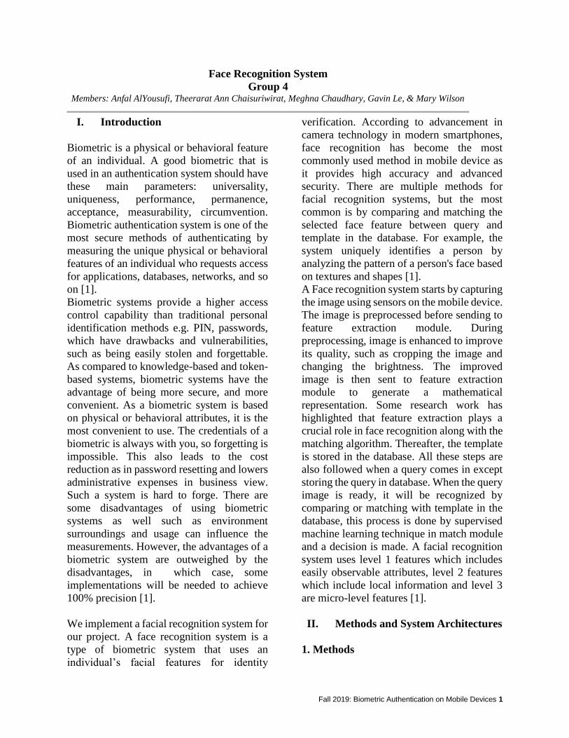
A. Feature Extraction
Facial feature extraction is the process of
extracting face component features like eyes,
nose, and mouth from human face image.
Facial feature extraction is essential for the
initialization of processing techniques like
face tracking, facial expression recognition
or face recognition [2]. Among all facial
features, eye localization and detection is
essential, from which locations of all other
facial features are identified [3]. The ability
to detect and describe salient features is also
an important component of a face recognition
system also.
A.1 Principal Component Analysis (PCA)
The main purposes of a principal component
analysis (PCA) are the analysis of data to
identify patterns and finding patterns to
reduce the computational complexity of the
dataset with minimal loss of information. In
general words, dimensionality is reduced by
using the Eigen face approach in PCA. They
are able to provide higher accuracy in
extracting facial features for human face
identification. PCA finds a linear projection
of high dimensional data into a lower
dimensional subspace. The Steps for the PCA
algorithm are the following:
● Step 1: Take the dataset consisting
old-dimensional samples by ignoring
the class labels.
● Step 2: Calculate third-dimensional
mean vector.
● Step 3: Compute the covariance
matrix of the dataset.
● Step 4: Calculate the eigenvectors of
the covariance matrix and
corresponding eigenvalues.
● Step 5: Sort the eigenvectors by
decreasing eigenvalues and choose k
eigenvectors with the largest
eigenvalues to form d x k dimensional
matrix W.
● Step 6: Use d x k eigenvector matrix
to transform the samples onto the new
sub-space.
For PCA matching, redo those steps with a
query image. Then match on the coefficients
in the projected space.
A.2 Local Binary Patterns Matching (LBPs)
Local Binary Patterns is used for facial
texture classification. The basic idea for
developing the LBPs operator was that two-
dimensional surface textures can be
described by two complementary measures
which are local spatial patterns and gray scale
contrast [4]. LBPs can be followed steps:
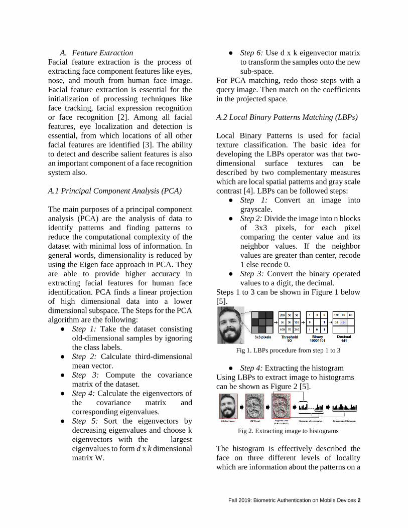
● Step 1: Convert an image into
grayscale.
● Step 2: Divide the image into n blocks
of 3x3 pixels, for each pixel
comparing the center value and its
neighbor values. If the neighbor
values are greater than center, recode
1 else recode 0.
● Step 3: Convert the binary operated
values to a digit, the decimal.
Steps 1 to 3 can be shown in Figure 1 below
[5].
Fig 1. LBPs procedure from step 1 to 3
● Step 4: Extracting the histogram
Using LBPs to extract image to histograms
can be shown as Figure 2 [5].
Fig 2. Extracting image to histograms
The histogram is effectively described the
face on three different levels of locality
which are information about the patterns on a

Fall 2019: Biometric Authentication on Mobile Devices 3
pixel-level, the labels are summed over a
small region to create information on a
regional level and the regional histograms are
concatenated to build a global description of
the face.
B. Random Forest Classifier
Random Forest Classifier is a bagging
technique. Bagging is another word for
Bootstrap Aggregation. In bagging, we use
the same dataset and create different models
from. The dataset. Random Forest Classifier
employs a number of decision trees. Each
decision tree works on a random sample of
data and gives an output for the classes. Each
tree’s decision is taken into account and the
final decision is based on averaging the
predictions. This also controls overfitting.
There are important parameters for each
classifier. In the case of Random Forests, we
can choose to change parameters such as
number of decision trees, the maximum depth
to which a tree can be grown and we can also
choose to get probabilistic predictions or log
probability predictions [6].
C. Feature Level Fusion
An image level fusion technique combines
different forms of images so that the
combined image contains more relevant
information than the individual ones [7].
There are three main types of fusion in
biometrics: decision, score, and feature level
fusion. Feature level fusion provides richer
information about the raw biometric data,
therefore making it produce better results [8].
Feature level fusion is simply the idea of
taking the feature set result from two
classifiers and putting them together before
putting them through a matcher function. In
our case, feature level fusion was done by
taking the feature set result from our PCA and
horizontally stacking (essentially
concatenating) it to the feature set result from
our LBP. From there, the horizontal stack of
both results is put through the matcher.
D. Image Enhancement
We can enhance the image in terms of
changing brightness, contrast, color and
sharpness. For image enhancement, we
separate our images in two parts: dark images
from task 6 to 10 are enhanced and images
from all other tasks are not enhanced. Images
from tasks 6 to 10 are the images captured in
dark environments For darker images, we
enhance them by brightening the images by a
factor of 20. We use ‘ImageEnhance’
module. First, we find all the filenames with
tasks 6 to 10. This is done by searching for
numbers 6 to 10. This also returned files with
16, 17, 18 and 19. So, we split the file name
and convert the string task number to integer
and choose only the images from tasks 6-10.
We brighten those images and merge them
into our images array.
2. System Architectures
A. System 1
System 1 is our control system. As shown in
Figure 3, the images were put through our
default image processor, then features are
extracted using PCA function, and then
classification is done using Random Forest
matcher.
Fig 3: System 1 Architecture
B. System 2
For system 2, we focused on how we could
alter the images to improve results from
system 1. As shown in Figure 4, the images
were put through our image enhancement
function before being put through the same

Fall 2019: Biometric Authentication on Mobile Devices 4
PCA then Random Forest. The idea for this,
as mentioned previously, was to separate our
darker images from the dataset, then enhance
(brighten in this case) the images by a factor
of 20.
Fig 4: System 2 Architecture
C. System 3
For system 3, we use the same images as
system 1, but decided to change the features
to be used. We did this with feature level
fusion of features derived using PCA and
LBP. As shown in Fig 5, the images are put
through the same default image processor as
system 1. Then the image features are
extracted using PCA and LBP functions, the
resulting features are fused together, then
Random Forest Classifier is used to generate
imposter and genuine scores. Also, we get the
probability based predictions for all our
systems.
Fig 5: System 3 Architecture
D. Three Trials of Three Systems
After testing our three systems, we decided to
try and change the number of trees our
Random Forest classifier uses. This showed
improvements, so in addition to our three
systems, we also tested each system with
three different number of trees for our
Random Forest Classifier. We tested each
system with 10, 50, and 100 trees. We left all
other parameters for the Random Forest
Classifier as the default.
E. Dataset
This experiment had five subjects, of which
all were asked to take videos of themselves
completing 25 tasks. Each video needed to be
about 30 seconds long. Most of the tasks
required the subject to record them standing
still will full face in view, limited pose and
limited expression. This was done in both
light and dark environments. Other tasks
included the subject moving around,
changing their expression or pose, wearing
face occlusions, or even talking with
someone in the background. The videos were
then put through a program to extract various
images. Between one and five images were
taken from each video. From there, the
images are ready to be used in our program.
III. Results
We test each of these systems with different
number of trees for analysis. We vary the
number of trees (i.e. number of components
from 10, 50 and 100), then we analyze how
the results vary by changing the number of
trees for each system. Therefore, we analyze
the systems in three parts. For the genuine
and imposter scores generated, we generate
150 different thresholds. We look at Score
Distribution Plots, Receiver Operating
Characteristic (ROC) curves and Detection
Error Tradeoff (DET) curves.
1. Part A - Random Forest with 10 Trees
A. System 1: Random Forest with PCA: We
get the score distribution plot as given in
Figure 6. In Figure 6, we observe d-prime
value of 1.46.
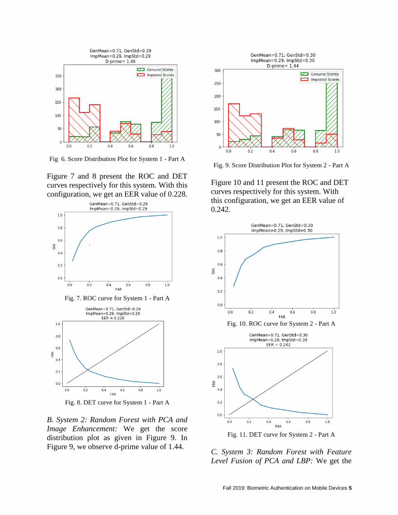
Fall 2019: Biometric Authentication on Mobile Devices 5
Fig 6. Score Distribution Plot for System 1 - Part A
Figure 7 and 8 present the ROC and DET
curves respectively for this system. With this
configuration, we get an EER value of 0.228.
Fig. 7. ROC curve for System 1 - Part A
Fig. 8. DET curve for System 1 - Part A
B. System 2: Random Forest with PCA and
Image Enhancement: We get the score
distribution plot as given in Figure 9. In
Figure 9, we observe d-prime value of 1.44.
Fig. 9. Score Distribution Plot for System 2 - Part A
Figure 10 and 11 present the ROC and DET
curves respectively for this system. With
this configuration, we get an EER value of
0.242.
Fig. 10. ROC curve for System 2 - Part A
Fig. 11. DET curve for System 2 - Part A
C. System 3: Random Forest with Feature
Level Fusion of PCA and LBP: We get the
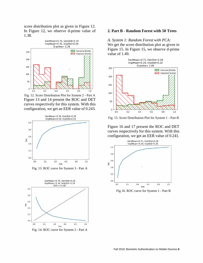
Fall 2019: Biometric Authentication on Mobile Devices 6
score distribution plot as given in Figure 12.
In Figure 12, we observe d-prime value of
1.38.
Fig. 12. Score Distribution Plot for System 2 - Part A Figure 13 and 14 present the ROC and DET
curves respectively for this system. With this
configuration, we get an EER value of 0.243.
Fig. 13. ROC curve for System 3 - Part A
Fig. 14. ROC curve for System 3 - Part A
2. Part B - Random Forest with 50 Trees
A. System 1: Random Forest with PCA:
We get the score distribution plot as given in
Figure 15. In Figure 15, we observe d-prime
value of 1.49.
Fig. 15. Score Distribution Plot for System 1 - Part B
Figure 16 and 17 present the ROC and DET
curves respectively for this system. With this
configuration, we get an EER value of 0.241.
Fig 16. ROC curve for System 1 - Part B

Fall 2019: Biometric Authentication on Mobile Devices 7
Fig 17. DET curve for System 1 - Part B
B. System 2: Random Forest with PCA and
Image Enhancement: We get the score
distribution plot as given in Figure 18. In
Figure 18, we observe d-prime value of 1.51.
Fig 18. Score Distribution Plot for System 2 - Part B
Figure 19 and 20 present the ROC and DET
curves respectively for this system. With this
configuration, we get an EER value of 0.238
Fig 19. ROC curve for System 2 - Part B
Fig. 20. DET curve for System 2 - Part B
C. System 3: Random Forest with Feature
Level Fusion: We get the score distribution
plot as given in Figure 21. In Figure 21, we
observe d-prime value of 1.49 .
Fig. 21. Score Distribution Plot for System 3 - Part B
Figure 22 and 23 present the ROC and DET
curves respectively for this system. With this
configuration, we get an EER value of 0.232.
Fig. 22. ROC curve for System 3 - Part B

Fall 2019: Biometric Authentication on Mobile Devices 8
Fig. 23. DET curve for System 3 - Part B
3. Part C - Random Forest with 100 Trees
A. System 1: Random Forest with PCA: We
get the score distribution plot as given in
Figure 24. In figure 24, we observe d-prime
value of 1.54 .
Fig. 24. Score Distribution Plot for System 1 - Part C
Figure 25 and 26 present the ROC and DET
curves respectively for this system. With this
configuration, we get an EER value of 0.236.
Fig. 25. ROC curve for System 1 -Part C
Fig. 26. DET curve for System 1 - Part C
B. System 2: Random Forest with PCA and
Image Enhancement: We get the score
distribution plot as given in Figure 27. In
Figure 27, we observe d-prime value of 1.54.
Fig. 27. Score Distribution Plot for System 2 - Part C
Figure 28 and 29 present the ROC and DET
curves respectively for this system. With this
configuration, we get an EER value of 0.232
Fig. 28. ROC curve for System 2 -Part C

Fall 2019: Biometric Authentication on Mobile Devices 9
Fig. 29. DET curve for System 2 - PartC
C. System 3: Random Forest with Feature
Level Fusion: We get the score distribution
plot as given in Figure 30. In Figure 30, we
observe d-prime value of 1.54.
Fig. 30. Score Distribution Plot for System 3- Part C
Figure 31 and 32 present the ROC and DET
curves respectively for this system. With this
configuration, we get an EER value of .
Fig. 31. ROC curve for System 3 -Part C
Fig. 32. DET curve for System 3 - Part C
We use Table 1 and 2 to compare between
performances of different systems under
different conditions.
System 1 System 2 System 3
Trees=
10
1.46 1.44 1.38
Trees=
50
1.49 1.51 1.49
Trees=
100
1.54 1.54 1.54
Table 1: Comparison of d-prime values for all the
systems
System 1 System 2 System 3
Trees=
10
0.228 0.242 0.243
Trees=
50
0.241 0.238 0.232
Trees=
100
0.236 0.232 0.224
Table 2: Comparison of EER values for all the
systems
IV. Conclusions

Fall 2019: Biometric Authentication on Mobile Devices 10
We tested three systems with random forest.
According to table 1 and 2 in the results
section, we can see that there is not much
difference in performance between system 1
and 2. Therefore, the image enhancement
does not affect the result in this project. On
the other hand, the EER value of system 3 in
the table 2 is lower than systems 1 and 2. In
addition, the higher of the number of trees in
Random Forest gives a higher d-prime and a
lower EER value. Thus, we can assume that
Random Forest with Feature Level Fusion as
well as the number of the trees allows for a
higher facial recognition accuracy.
This project has allowed us an in depth
experience of how a facial recognition
system works. We learned which systems
help for better performance and what to
change to improve our results. In the future,
our team will do more research on other
feature extractors and matchers to improve
the system accuracy. In addition, we want to
improve our image enhancement function to
improve performance for system 2.
V. References
[1] Chapter 1: Introduction Jain, Anil K., Arun A. Ross, and
Karthik Nandakumar Introduction to biometrics. Springer
Science & Business Media, 2011. Access:
http://ezproxy.lib.usf.edu/login?url=http://link.springer.com
/10.1007/978-0-387-77326-1
[2] Benedict, S. R., & Kumar, J. S. (2016). Geometric
shaped facial feature extraction for face recognition. 2016
IEEE International Conference on Advances in Computer
Applications (ICACA), 275–278.
[3] Feature Extraction in Face Recognition: A Review.
(2018). Retrieved October 21, 2019, from UKEssays.com
[4] Ojala, T., Pietikäinen, M., & Harwood, D. (1996). A
comparative study of texture measures with classification
based on featured distributions. Pattern Recognition, 29(1),
51–59.
[5] Prado, K. S. do. (2018, February 3). Face Recognition:
Understanding LBPH Algorithm. Retrieved October 23,
2019.
[6]https://scikit-
learn.org/stable/modules/generated/sklearn.ensemble.Rand
omForestClassifier.html
[7] Dey, A., & Sing, J. K. (2015). An image fusion technique
for efficient face recognition. 2015 IEEE 2nd International
Conference on Recent Trends in Information Systems
(ReTIS), 261–266.
[8] Ross, A. A., & Govindarajan, R. (2005, March). Feature
level fusion of hand and face biometrics. In Biometric
Technology for Human Identification II (Vol. 5779, pp. 196-
204). International Society for Optics and Photonics.

Project 1 - Report PCA with KNN and NB Matching Group 5
Introduction Biometrics is technological way to identify people through identification and authentication. This can be through a person's knowledge, such as a password, something they possess such as a key, and their physical and behavioral attributes such as face recognition or gait. A biometric system is made up of different sections: Sensor modules which measures and records the raw biometric data; Feature extraction which generates a compact and expressive digital representation, or a template, and then enrolls it into the system; Database which stores templates and retrieves the query, which is a person wishing to be recognized; Matching, where the differences between the query and template are measured [3]. One way to identify people biometrically is through face recognition. Face recognition establishes someone based on their facial characteristics that are unique and identifiable. A person’s face is commonly used because it is suitable for non-contact sensors, it has the “big 7” (universality, uniqueness, permanence, measurability, performance, acceptability, and circumvention) properties of a good biometric modality, and the front-facing cameras of modern smartphones are of reasonable quality sufficient for verification [5]. In developing a face recognition system, “there exists a wide variety of sensors available for data collection on the smartphone ranging from physical to environmental to movement to location to interactive” [3]. In our project, we developed a face recognition system that used Principal
Component Analysis (PCA) as a feature extraction, which “maps the high dimensional face image into a lower dimension defined by a subspace of basis vectors...also called eigenfaces” [5]. We then took those eigenfaces and used k-Nearest Neighbors (KNN) and Naive Bayes (NB) matching algorithms to compare our sets of faces between each other to see how well it could match one person to their own face, i.e. Shanice to Shanice’s face would be genuine versus Shanice to Anna’s face would be impostor. We focused on two main sets of images (tasks), referred to as the “Emotion” tasks, and “Motion” tasks. Emotion tasks focused on the faces that had limiting pose (the subject was stationary) but the expressions changed depending on the task. Motion tasks focused on the images in which the subject was moving and also included images where the target individual was accompanied by someone that was not one of our four group members. We compared female versus female faces, male versus male faces, and female versus male faces. Our goal in comparing these different sets of faces is to see which group of faces our face recognition system will give the best results and where it gives the worst results. In this report, we will describe the multiple methods we used in our face recognition system, the different system architectures that were used including our chosen datasets, the results we got from our system performance analysis, and finally our conclusions from this experiment.
Fall 2019: Biometric Authentication on Mobile Devices 1

Methods There were two main sections to our face recognition system. Feature extraction is the first of these sections and matching algorithms is the second. Below, we explain the methods used and why we chose these methods. First, the dataset was split into two categories, Motion and Emotion. Motion tasks consisted of tasks that involved movement in some type of way or a person not in the group being in the frame. These tasks are described in detail below.
● Task 15 - While facing the camera, with individual’s full face in the frame in a fully lit indoor environment while walking.
● Task 16 - While facing the camera, with individual’s full face in the frame in a fully lit indoor environment while jogging.
● Task 20 - While facing the camera, fully in the frame, the individual is moving in and out of the frame by rocking side to side (left to right, right to left) in a fully lit indoor environment.
● Task 23 - While facing the camera, the individual is talking to someone that is standing right beside them in a fully lit indoor environment, both individuals needed to be visible in the frames. It is acceptable to for one or both of the faces to be partially in the frame.
● Task 24 - While facing the camera, the individual is talking to someone that is standing 10 feet behind them in a fully lit indoor environment. Both individuals needed to be visible in the frames. It is acceptable to for one or both of the faces to be partially in the frame.
Emotions consisted of tasks that involved the individual being in a stationary position but each task showing some different types
of Emotion (neutral, sad, etc.). These tasks are described in detail below.
● Task 1 - While facing the camera, with the individual’s full face in the frame, limiting pose, in a fully lit indoor environment.
● Task 11 - While facing the camera, with the individual’s full face in the frame, limiting pose, in a fully lit indoor environment while expressing laughing (as naturally as possible).
● Task 12 - While facing the camera, with the individual’s full face in the frame, limiting pose, in a fully lit indoor environment while expressing anger (as naturally as possible).
● Task 13 - While facing the camera, with the individual’s full face in the frame, limiting pose, in a fully lit indoor environment while expressing shock or surprise (as naturally as possible).
● Task 14 - While facing the camera, with the individual’s full face in the frame, limiting pose, in a fully lit indoor environment while expressing sadness (as naturally as possible).
The feature extraction method used was PCA which is used to identify the major directions and the corresponding strengths of variation in the data [1]. With the use of PCA, we extract the eigenfaces. “The eigenfaces are a reconstruction of the original faces by taking some of each eigenface” [6]. In Figure 1A we have a set eigenfaces for the set of Motion and in Figure 1B we see a set of eigenfaces for the set of Emotion tasks .
Fall 2019: Biometric Authentication on Mobile Devices 2

Figure 1A: Eigenfaces for motion tasks.
Figure 1B: Eigenfaces for emotion tasks.
We used three different categories to analyze our data which are described in greater detail in the “System Architecture” section of this report. Each category was compared using two different matching techniques. The first technique was the KNN classifier. It is a type of instance based learning where the function is only approximated locally, and all computation is delayed until classification. The K refers to the number of nearest neighbors that the classifier will use to make its prediction. “It is used to classify unlabeled observations by assigning them to the class of the most similar labeled examples”[8]. We chose KNN because it is a commonly used matching technique. The second was Naive Bayes, specifically Gaussian Naive Bayes. “A Bayesian network consists of a structural model and a set of conditional probabilities” [2]. It is used to measure the probability of an event based on the previous knowledge of the event. We used this model to have an additional metric to compare in our analysis. One of our goals was to compare the results from the two matching techniques and see which one produced a more accurate result.
System Architectures For this project, we focused on three architectures: PCA, KNN, and NB. PCA was used to get the features that were then used in our matching algorithms. The matching algorithms used were the KNN and Naive Bayes algorithms for classification. We later use the genuine and imposter scores from these matching algorithms to determine the performance by computing the False Acceptance Rate (FAR), False Reject Rate (FRR), and True Positive Rate (TPR). These values were also used to determine the Equal Error Rate (EER), compute the Detection Error Tradeoff (DET), and Receiver Operating Characteristics (ROC) curves, as well as plotting the score distribution for the individuals. For our experiment, we have decided to compare the faces of each of the four members in our group with each other. The members of the group consist of 2 males and 2 females. An analysis was made based on the following criteria:
● Male and Female ○ Anna and Jose ○ Shanice and Jose ○ Anna and Khaled ○ Shanice and Khaled
● Female and Female ○ Anna and Shanice
● Male and Male ○ Jose and Khaled
For this analysis, we had four test subjects who had 5 images for 25 tasks. Due to the structure of the analysis, we chose to only include the images for 10 different tasks which are stated above. We also did the analysis comparing two individuals at a time. This means that for each analysis there were 50 images being analyzed. This number varied between 26 and 50 images depending on which two subjects were being compared due to FTC images in the dataset. The FTC images were ignored and
Fall 2019: Biometric Authentication on Mobile Devices 3

no specific number was chosen to run all iterations the same way. A total of 6 tests were conducted where each test conducted was a comparison between one individual with another. Ex: Khaled was compared with Shanice (Figure 2A). Later, Khaled was compared with Jose (Figure 2B). Then Khaled was compared with Anna (Figure 2C). These steps were repeated for each member.
Figure 2A: Images of Khaled and Shanice from the Motion dataset, Task 24 - Facing
the camera, while talking to someone that is standing 10 feet behind in a fully lit indoor
environment. Both individuals needed to be visible in the frames.
Figure 2B: Images of Khaled and Jose from the Emotion dataset, Task 11 - Facing the camera,full face in the frame, limiting pose,
in a fully lit indoor environment while expressing laughing (as naturally as
possible).
Figure 2C: Images of Khaled and Jose from
the Emotion dataset, Task 14 -Facing the camera, full face in the frame, limiting pose,
in a fully lit indoor environment while
expressing sadness (as naturally as possible).
To get the PCA features from our images in the dataset, we “squash” the images so that they are represented as vectors. The mean value for the faces is computed and the data in the vectors are standardized by subtracting the mean. The covariance matrix was computed as C = A’A where A is the image matrix [6]. The next step was to compute the eigenvalues and eigenvectors from the covariance matrix. This step also includes mapping the eigenvectors back to the image dimensions. We took the top five eigenvectors with the five highest PCA components to use with the KNN and Naive Bayes classifiers [6]. For the KNN classifier, the distance metric that was chosen was the ‘manhattan’ distance. We also ran a different number of experiments which used different values for the number of neighbors, ranging from 1 neighbor to 45 neighbors. One limitation KNN provides is that the number of neighbors k cannot be larger than the number of samples in the dataset. The largest number of samples we could have was 50 so k could not be larger than 50. Only an odd number of neighbor(s) was chosen to avoid ties during voting. We looked at a variety of values for k to find out which would be the optimal choice for our system. When using values for k that are small, the distribution of the training data is ignored [4] and noise will have a higher impact on the result [7]. When k is a larger value, the distribution of the data is considered but when the value is too large the classifier will underfit [4]. It was necessary to choose a number of neighbors k that avoided both of these situations. For the Emotion dataset we chose a k value of 19 while for the Motion dataset we chose a k value of 5. Our observations as to why
Fall 2019: Biometric Authentication on Mobile Devices 4

these numbers were chosen are specified in our “Results” section. The ‘Manhattan’ distance from the unlabeled data sample and each data point was computed. Majority voting on the k data points with the shortest distance to the unlabeled sample determined the class of the sample. During the planning of this experiment, we were initially going to only run KNN but decided to also run naive bayes to compare the results from the two algorithms and analyze how the two performance results differ. For the naive bayes analysis, we used the Gaussian Naive Bayes (GNB) algorithm for classification.[4] The Gaussian Naive Bayes algorithm we utilized image and label lists. The classifier was trained and later used to predict the label of a query. From this prediction, the algorithm returned genuine and impostor scores which were later used in the performance analyzer.
For our performance analysis, we first computed the False Acceptance Rate (FAR), False Reject Rate (FRR), and True Positive Rate (TPR). To do this we used the genuine and imposter scores that were captured using either the KNN or GNB matcher algorithms. With those scores and a specified number of thresholds of 150, scores were then classified as true positive (TP), false positive (FP), true negative (TN), or false negative (FN). Using these values and threshold values, the FAR, FRR, and TPR are able to be calculated. The EER for each comparison was also calculated by using the FAR and FRR values. Once all scores were calculated, we were able to plot the DET and ROC curves and also produce the score distribution charts.
Results KNN - Emotion For the Emotion datasets we chose a KNN value of 19 because among the 6 datasets this number showed the best and consistent EER for each one. Figure 3A-3C shows the data received for Female and Male (Anna and Jose):
Figure 3A: Anna and Jose Dataset score
distribution
Figure 3B: Anna and Jose Dataset ROC
Curve
Figure 3C: Anna and Jose DET Curve
Our d-prime value was 17.56 which is good, because the higher the d-prime value the higher amount of separation there is between the genuine and impostor curves.
Fall 2019: Biometric Authentication on Mobile Devices 5

The ideal value for ROC is at (1,0), and the ideal EER is 0.000. As seen in Figure 3B and 3C, these values are both seen in our data. This means that our face recognition was highly accurate in distinguishing between these female and male eigenfaces. Figures 4A-4C shows the data received for Female and Female (Anna and Shanice):
Figure 4A: Anna and Shanice score
distribution
Figure 4B: Anna and Shanice ROC curve
Figure 4C: Anna and Shanice DET Curve
Our d-prime value for this dataset is 6.71 which is lower than the female and male dataset, and the genuine and impostor curves are closer together because of this. There is still a separation but not as distinct, and there is some overlap of false negatives
and false positives. The ROC value is not perfect like being at (1,0). Our DET value is also not a perfect 0.000, but 0.023. It seems our system has a harder time comparing female to female faces compared to male to male. Figures 5A-5C shows the data received for Male and Male (Jose and Khaled):
Figure 5A: Jose and Khaled score
distribution
Figure 5B: Jose and Khaled ROC curve
Figure 5C: Jose and Khaled DET Curve
Our d-prime value for Jose and Khaled is an infinitely large number, so the curves are far apart which is good. Our system seems to be very accurate when it comes to identifying male to male eigenfaces. The ROC Curve and DET curve show perfect
Fall 2019: Biometric Authentication on Mobile Devices 6

values for this dataset. Also, we found that no matter what knn value we used for this specific dataset the DET value always came out a perfect value of 0.000 meaning our face recognition system is highly accurate for this specific male to male comparison. KNN - Motion When using the KNN classifier for tasks that involve motion, we found that lower values for the number of neighbors gave the best results (lowest EER values). The images for the motion tasks were classified using five nearest neighbors. The downside to this is that having a small value for k could mean that our classifier is subject to noise and that it is ignoring the distribution of our training data [4]. Another interesting observation that we made when analyzing our results was the difference in the amount of separation in the scores that resulted from classifying male and male and female and female. Figures 6A and 6B show the score distributions of Anna and Shanice and Jose and Khaled.
Figure 6A: Anna and Shanice Score
Distribution
Figure 6B: Jose and Khaled Score Distribution
The higher d-prime value for Jose and Khaled (2.73) and lower EER value (0.114) compared to Anna and Shanice (d-prime: 1.25 and EER: 0.148) shows that the classifier also had a harder time distinguishing between female and female for the motion tasks just as it did for the emotion tasks.
Figure 7A: Khaled and Shanice Score Distribution
Fall 2019: Biometric Authentication on Mobile Devices 7

Figure 7B: Khaled and Shanice ROC
Figure 7C: Khaled and Shanice DET The classification of Khaled and Shanice gave the best EER result for the motion tasks. The separation between the genuine and impostor scores (dprime: 2.31) was not as high as the separation for Jose and Khaled (dprime: 2.73) but the EER was higher (0.081 and 0.114).
Figure 8A: Jose and Shanice Score Distribution
Figure 8B: Jose and Shanice ROC
Figure 8C: Jose and Shanice DET
The highest EER value for KNN on motion tasks came from comparing Jose and Shanice. Figure 8A shows that there is a lot of overlap between the genuine and impostor scores which would lead to higher false positives and false negatives depending on the decision threshold. This classification did give us higher false accept rate than false reject rate. Naive Bayes - Emotion For the Emotion dataset, we also chose to implement the Naive Bayes method among the 6 datasets. Figure 9A-9C shows the data received for Female and Male (Anna and Jose):
Fall 2019: Biometric Authentication on Mobile Devices 8

Figure 9A: Anna and Jose score
distribution
Figure 9B: Anna and Jose ROC curve
Figure 9C: Anna and Jose DET Curve
When analyzing the results from figure 9A, we can see that we have a very high D-Prime, this indicates the separation between the genuine and imposter. This means that the higher the D-prime the better since the genuine is farther away from the imposter. When looking at the ROC curve in figure 9B, we can see that the
curve is closed to 1, making it more accurate. We can also see that the genuine mean it is at 1 which is good. In figure 9C, we can see that there is 0.00 EER rate, which means that our facial recognition system is highly accurate when classifying Anna and Jose while using Naive Bayes. Figures 10A-10C shows the data received for Female and Female (Anna and Shanice):
Figure 10A: Anna and Shanice score
distribution
Figure 10B: Anna and Shanice ROC curve
Fall 2019: Biometric Authentication on Mobile Devices 9

Figure 10C: Anna and Shanice DET Curve When analyzing the results from figure 10A, we can see a D-Prime that is not as high as the D-prime from figure 9A, but it is significantly high enough to generate perfect scores. In figure 10B, we can see that the ROC curve is close to TAR = 1, making this a good classifier. We can also see that the genuine mean it is at 1 which is good. In figure 10C, we can see that there is 0.00 EER rate, which means that our facial recognition system is highly accurate when classifying Anna and Shanice while using Naive Bayes. Figures 11A-11C shows the data received for Male and Male (Jose and Khaled):
Figure 11A: Jose and Khaled score
distribution
Figure 11B: Jose and Khaled ROC curve
Figure 11C: Jose and Khaled DET Curve
When analyzing the results from figure 11A, we can see a D-Prime which is not as high as the D-prime from figure 9A or figure 10A, but it is high enough to generate perfect scores. In figure 11B, we can see that the ROC curve is close to TAR = 1, making this a good classifier. In figure 10C, we can see that there is 0.00 EER rate, which means that our facial recognition system is highly accurate when classifying Jose and Khaled while using Naive Bayes. Naive Bayes - Motion For the Motion dataset, we chose to implement the GNB matching method among the 6 datasets. Figures 13A-13C shows the data received for Female and Male (Anna and Jose):
Fall 2019: Biometric Authentication on Mobile Devices 10

Figure 12A: Anna and Jose score
distribution
Figure 12B: Anna and Jose ROC curve
Figure 12C: Anna and Jose DET curve
Our Score distribution graphs shows great results in that we have a good D-prime value of 3.64. We also got a great genuine mean of 0.93 and low impostor mean of 0.07. Our EER was low at 0.059 which shows less than 1% Equal Error Rate. Figures 14A-14C shows the data received for Female and Female (Anna and Shanice):
Figure 13A: Anna and Shanice Score
Distribution
Figure 13B: Anna and Shanice ROC curve
Figure 13C: Anna and Shanice DET curve Our Score distribution graphs shows great results in that we have a good D-prime value of 4.64. We also got a great genuine mean of 0.94 and low impostor mean of 0.06. Our EER was low at 0.074 which shows less than 1% Equal Error Rate. This means that for female and female, we get a higher D-Prime value than Male and Male as well as a higher genuine mean but also a higher EER.
Fall 2019: Biometric Authentication on Mobile Devices 11

Figures 15A-15C shows the data received for Male and Male (Jose and Khaled):
Figure 14A: Jose and Khaled Score
Distribution
Figure 14B: Jose and Khaled ROC curve
Figure 14C: Jose and Khaled DET curve
Our Score distribution graphs shows great results in that we have a good D-prime value of 13.0. We also got a great genuine mean of 0.97 and low impostor mean of 0.03. Our EER was a perfect 0. This means that for our Male and Male analysis, we get the most accurate results.
Conclusions In our analysis we found that while using the KNN classifier, our system had an easy time comparing Male to Male, and Female to Male eigenfaces; however, it had a more difficult time comparing Female to Female eigenfaces which was interesting. While when using the Naive Bayes method on the Emotion dataset, we noticed that the Males and Males had the lowest D-prime compared to Female and Male and Female and Male. Regardless, the D-prime for Male and Male was still large enough for a perfect classification. Most of our finding’s DET Curve values turned out to be 0.000 which means our system is highly accurate. Some limitations we found was our low sample size and also some of the samples we had we could not use since they had a failure to capture error. For the Motion dataset, some individuals data images had more impostor images than the individuals themselves. We were able to get good results from our datasets since the number of samples was low, it would be interesting to see how this system of PCA using KNN and NB matching using larger sample sizes in future works. References [1] Chen, T., Hsu, Y. J., Liu, X., & Zhang, W.
(2002, September). Principal component analysis and its variants for biometrics. In Proceedings. International Conference on Image Processing (Vol. 1, pp. I-I). IEEE.
[2] Jiang, L., Wang, D., Cai, Z., & Yan, X. (2007, August). Survey of improving naive bayes for classification. In International Conference on Advanced Data Mining and Applications (pp. 134-145). Springer, Berlin, Heidelberg
[3] Neal, T. (2019). CIS4930. Biometric Authentication on Mobile Devices, week 1, lecture 1.
Fall 2019: Biometric Authentication on Mobile Devices 12

[PowerPoint Slides]. Retrieved from https://usflearn.instructure.com/courses/1347065/files/folder/Lectures?preview=82180628
[4] Neal, T. (2019). CIS4930. Overview of Python and Machine Learning, week 2, lecture 2A. [PowerPoint Slides]. Retrieved from https://usflearn.instructure.com/files/82698356/download?download_frd=1
[5] Neal, T. (2019). CIS4930. Face Recognition, week 5, lecture 4. [PowerPoint Slides]. Retrieved from https://usflearn.instructure.com/courses/1347065/files/folder/Lectures?preview=83522204
[6] Dr. Neal, T. (2019). CIS4930. Principal
Component Analysis, week 6, lecture 5. [PowerPoint Slides]. Retrieved from https://usflearn.instructure.com/files/83751094/download?download_frd=1
[7] Thirumuruganathan, S. (2010). A Detailed Introduction to K-Nearest Neighbor (KNN) Algorithm. Retrieved from https://saravananthirumuruganathan.wordpress.com
[8] Zhang, Z. (2016). Introduction to machine learning: k-nearest neighbors. Annals of translational medicine, 4(11).
[9] 1.9. Naive Bayes. (n.d.). Retrieved from https://scikit-learn.org/stable/modules/naive_bayes.html#gaussian-naive-bayes.
Fall 2019: Biometric Authentication on Mobile Devices 13

Comparing Classifiers and Block Sizes Used with Local Binary Patterns Group 6
Introduction As our lives continue to rely more and more on technology, our personal information is steadily becoming more sensitive. With everything from shopping to online banking just a click away, the need for security to protect our personal information is crucial. A solution to this is biometrics. Biometrics are defined as unique physical characteristics, such as fingerprints, that can be used for automated recognition [1]. Biometric traits fall into two categories; physical and behavior. Some examples of physical traits are fingerprints, face, iris, DNA, and periocular regions. Behavioral traits include voice, gait, and signature. These characteristics are collected and input into a biometric system for recognition.
A biometric system is made up of several modules including a sensor module, a feature extraction module, a database, and a matching module. The system begins in the sensor module. If a person is a new user to the biometric system, the user will provide data to the system and the data will be stored as a template in the database for that user. After a person has used the system for the first time, subsequent uses will collect the data as a query. The query is then enhanced and passed into the feature extraction module. The template is retrieved from the database and the extracted features and the template are passed into the matching module. The feature and the template are compared and based on a given criteria and a decision is made whether the user is genuine or an imposter.
Biometric systems have different methods of comparing a query to template called authentication and identification. Authentication is when a query is compared directly to a template to find out if a user is who they say they are. Identification is when a query is compared to every template in a
database to find out if the user is someone who is known in the system.
The focus of this experiment is facial authentication. The features of a person’s face can be extracted in many ways including placing landmarks on an image, collecting features with Principal Component Analysis(PCA), which measures the variance between the template and the query, and Local Binary Patterns(LBP) which divides an image into mxm blocks, where m = block size, and each block is divided into 3x3 pixel blocks. The center pixel is then compared to all of its neighbors and an eight digit binary code is generated and converted to a decimal number. These blocks of numbers create histograms that can be concatenated to find the resulting features. These features are then passed to a matcher to determine if the subject is genuine or an imposter.
Figure 1: LBP Process
In this experiment, a dataset of 585 images were used to capture LBP features with varying block sizes. Five sets of LBP features were gathered from each image divided into block sizes of 4, 8, 12, 16, and 20. The collected features were then passed to two matchers, one using a K-Nearest Neighbor classifier with 10 neighbors and measuring Manhattan distance and the other using a Gaussian Naive Bayes classifier. Each set of results were then compared to see how variations in the block size of LBP features impact the accuracy of the facial recognition system.
Fall 2019: Biometric Authentication on Mobile Devices 1

System Architectures For these tests, we compare Local Binary Patterns (LBP) feature extraction when implemented with different classifiers. This assessment compares a system that uses LBP features and K-Nearest Neighbors (KNN) classification, to a system that uses LBP features and Naive-Bayes (NB) classification system.
We also compare how the system implementations vary depending on the block size used for LBP. We used five different block sizes for LBP i.e 4, 8, 12, 16 and 20. To elaborate, we have two systems for a block size of 8: one with the K-Nearest Neighbors (KNN) classifier, and another one with the Naive Bayes (NB) classifier. This brings us to a total of 10 total systems, referred to in the order of smallest to greatest with KNN first and NB second. For instance, what we refer to as our fourth system would be an LBP system which uses a block size of 8 and an NB classifier. The outputs which we obtain from this experiment is genuine mean, genuine standard deviation, impostor mean, impostor standard deviation and equal error rate(EER) using KNN and NB classifiers.
KNN Class. NB Class.
4 Blocks System 1 System 2
8 Blocks System 3 System 4
12 Blocks System 5 System 6
16 Blocks System 7 System 8
20 Blocks System 9 System 10
Figure 2: Systems by Block Size and Classifier used
In our first method we used LBP for the facial feature extraction, and for KNN for image classification. LBP has many important properties, such as its robustness
against any monotonic transformation of the gray scale, and its computational simplicity, which makes it possible to analyze images in challenging real-time settings. The greater accuracy of KNN in image classification problems is highlighted; it is commonly used for its easier interpretation and low calculation time. The main aim of LBP and KNN in this work is to extract features and classify different LBP histograms, respectively, in order to ensure good matching between the extracted features histograms and provide a greater identification rate.
For this LBP and KNN approach, we used the data collected from my team, and preprocessed the data which we collected. Faces are localized and converted to greyscale in the preprocessing stage. In the first stage, we collected the extraction features using the LBP algorithm. In the second stage, we classify using the KNN algorithm with manhattan distance. Finally authentication process is completed by this process.
Figure 3: LBP and KNN Approach
In our second method to get facial feature extraction, we again used LBP and for image classification we used another classification algorithm Naive-Bayes(NB). Feature is extracted using the LBP
Fall 2019: Biometric Authentication on Mobile Devices 2

approach used above and classification is done using NB classifier which is based on the Bayesian theorem. It is particularly suited when the dimensionality of the inputs is high. Parameter estimation for Naive Bayes models uses the method of maximum likelihood.
Figure 4: LBP and NB Approach
For this LBP and NB approach, we used the data collected from the team, and preprocessed the data which we collected similar to the first approach i.e LBP and KNN approach. In the first stage, we collected the extraction features using the LBP algorithm. In the second stage, we classify using the NB algorithm. Thus authentication process is completed by this process.
The data for this experiment was gathered from four people who recorded 25 videos of themselves in various situations. These situations varied in the environment, facial expressions, lighting, movement, obstructions, as well as including other people. Images were extracted from certain frames of these videos. These images were converted to grayscale and used to gather landmarks for the faces in the images. Some images were discarded as they could
not be utilized for this experiment due to problems such as poor light conditions. The amount of images per subject ranged from 125-207 per subject, with a total of 585 images and an average of 146 per person.
There were also instances in the database when the images pulled from the videos happened to be a different person than the subject, who appeared in the background. These instances may have played a role in gauging the accuracy of the system.
The remaining usable images of the database would then be imported to our systems to provide our accuracy results.
Results Our images were first converted into histograms and then concatenated to form an image of LBP features. An example of the resulting image is displayed in figure 1.1. The resulting images were then passed to the KNN and NB classifiers. The results show that as the block size increases, the accuracy of the matcher also increases. The K-Nearest Neighbor classifier produced significantly better results than the Naive Bayes classifier.
Figure 5: Concatenated LBP histograms
Due to the amount of results from this experiment, tables with all quantitative
Fall 2019: Biometric Authentication on Mobile Devices 3

results have been created for each classifier and graphs have been included in a separate folder. The results collected from each classifier are as follows:
Block size 4 8 12 16 20
Gen. mean
0.58 0.60 0.64 0.65 0.65
Gen. Std
Dev.
0.26 0.24 0.24 0.23 0.23
Imp. Mean
0.42 0.40 0.36 0.35 0.35
Imp. Std. Dev.
0.26 0.24 0.24 0.23 0.23
EER 0.392 0.397 0.326 0.286 0.286
Figure 6: KNN Results
Block size 4 8 12 16 20
Gen. mean
0.01 0.05 0.09 0.20 0.20
Gen. Std
Dev.
0.11 0.23 0.29 0.40 0.40
Imp. Mean
0.99 0.95 0.91 0.80 0.80
Imp. Std. Dev.
0.11 0.23 0.29 0.40 0.40
EER 0.988 0.945 0.908 0.798 0.798
Figure 7: NB Results
As each table shows, the NB classifier is extremely inaccurate. It can be said that when comparing LBP features for facial recognition, a KNN classifier is preferred. Although the experiment only has a range of
block sizes from 4 - 20 blocks, based on the results of 16 and 20 blocks it appears that the accuracy plateaus at 16 blocks. This shows that block size can only be increased up to a certain point before it is no longer beneficial to the accuracy of the system.
Certain images may have been harder to classify based on the images environment or similar affecting conditions. This may include pictures with obstructions or poor light conditions. The system may have a hard time classifying such images since it could not correctly determine the subject presented.
Conclusion In this experiment, our goal was to find out if we could increase the reliability of a facial recognition system by changing some variables within the system. Those variables in question are (1) the number of blocks in an image for local binary patterns (LBP) feature extractor and (2) the use of K-nearest neighbors (KNN) versus naïve Bayes as classifier for the system. We compared systems where LBP divided images into 4 blocks, 8 blocks, 12 blocks, 16 blocks, and 20 blocks. For each number of blocks for the LBP, we also compared both classifiers. There was a total of 10 systems. The results show that as the block size for LBP increases, so does the accuracy of the matcher. This is true regardless of the classifier used. One possible explanation for this is that there is more variation in the LBP histogram for each block. A larger block size can generate a histogram that stores data for a larger area of the original image. Therefore, small minute details do not influence the outcome as much. Throughout this experiment, we learned that out of the architectures we examined, a higher block size, around 20, paired with a matcher that uses a KNN classifier is
Fall 2019: Biometric Authentication on Mobile Devices 4

optimal for facial authentication. Because our main focus was to assess the effect LBP block size has on the system, we wanted to keep all other factors constant (with the exception of the matcher) so we did not employ any enhancement techniques to the images. While our best architecture yielded decent results, it is nowhere near good enough to deploy for actual use. Other areas of the architecture that we would like to explore are (1) the use of fusion techniques to combine the results of both classifiers, or use an entirely different classifier altogether, and (2) using image enhancement during the preprocessing stage. If the template and query images are taken in different environments, noise such as lighting or motion blur will affect the performance. Image enhancement can minimize this effect. This experiment did not have any major limitations, as we were simply assessing the effect different block sizes have on the system. We were able to keep all other factors constant and get good results. References [1] “Biometrics,” Department of Homeland Security, 09-May-2019. [Online]. Available: https://www.dhs.gov/biometrics. [Accessed: 26-Oct-2019].
[2] I. L. K. Beli and C. Guo, “Enhancing Face Identification Using Local Binary Patterns and K-Nearest Neighbors,” Journal of Imaging, vol. 3, no. 3, p. 37, Sep. 2017.
[3] N. S. Sarode and A. M. Patil, “Iris Recognition using LBP with Classifiers-KNN and NB,” Iris Recognition using LBP with Classifiers-KNN and NB, vol. 4, no. 1, pp. 1904–1908.
Fall 2019: Biometric Authentication on Mobile Devices 5

Face Recognition - FTC vs NFTC Group # 7
Introduction Biometrics is the measurement and analysis of unique physical or behavioral characteristics found in a person, which is used as vital data in order to verify or identify an individuals identity. Physical characteristics are considered attached to the person, such examples include face, fingerprints, iris, hand, DNA and periocular. Behavioral characteristics are pattern based behaviors related to the person, such as keystroke, gait, signature and voice. These biometrics all come together to help build upon the known system for user authentication, the biometrics system. The biometrics system is a technological system that uses information about a person to identify them. They rely on biometric data collected from the user, in which is used to clarify the identity of the query. This system can be described also as the division of four functioning components, which work together to generate this system. The first component known to the system is the Sensor Module. A sensor module includes the measurement of raw biometric data, where the data includes traits such as face, fingerprint, and iris. The second component, feature extraction, creates a digital representation, called a template, that is stored or enrolled in a database. The third component, known as the Database, contains the stored templates and is used to retrieve a query, the individual that wants to be authenticated. The final component, Matching, uses both the database and feature extraction to be able to proceed with applying its own unique process. Matching measures the likeness or dislikeness between the query and template. Using all of these components that make up a biometric system, we can apply face recognition. Face recognition is an
application of this biometric system which can identify or authenticate a person based on the features of their face [3]. Face recognition is misinterpreted sometimes for face detection, in which detection is has the objective of locating the faces in an image and use them for the face to face recognition system [3], but differs from recognition which has the facial images already extracted from the images, and is usually converted to grayscale in which the face recognition algorithm is responsible for searching the image processed for certain characteristics that define the portrait image [3]. With technological advances every other year, we are able to apply face recognition more efficiently for different uses within our lives. Such uses for face recognition would include security purposes such as airports, banks, highly populated areas such as malls and entertainment locations. It’s most popular use is smartphone authentication, in which the owner of his/her phone has the ability to unlock their mobile device through the recognition of their own face. It’s also currently being used consistently with home security purposes, in which access to the house may only be unlocked for recognizable people through their camera systems. There are reasonable limits behind face recognition which include costs and technology requests, in which given time, we shall prosper with increasing its use within our lives and have full confidence of its security and reliability to successfully complete its job. Methods
Fall 2019: Biometric Authentication on Mobile Devices 1

There are many feature extraction methods known to be able to implement face recognition based on a certain method. For the purposes of our project, we were able to select two popular methods and applied them to our algorithms, and they are known as Local Binary Pattern (LBP) and Principal Component Analysis (PCA). Principal component analysis (PCA) is a technique used to emphasize variation and bring out strong patterns in a dataset. It's often used to make data easy to explore and visualize[1]. This method has multiple steps in which the process must uphold in order to complete correctly and ensure accuracy with the data. The first step would be gathering the images of interest, that are considered matrices, in which they shall be delivered to the next step of this process. The second step would be ‘squashing the images’ (as seen in figure 1), in which we are able to reduce the size of the portained image.
Figure 1: PCA - Reducing image size This step of squashing allows us to transform the image and represent it as a vector. We complete this step for all images, reducing their size and gathering our multiple newly created vectors. Once completed, we are able to standardize the data, which is done by computing the mean face found from these images seen as vectors, and subtracting the mean face from each image. The third step would be to gather the standardized data, and compute
the covariance in the data. Covariance of a matrix is multiplying the matrix features by its transpose. The reason behind using a covariance matrix is due to the matrix accounting for variability in the dataset. To explain this more, converting the image will definitely have an impact on the amount of variance in data loss, which may have an impact on the recognition process. The original image will account for the entire variability based on all the components for the image and all the variables. PCA will reduce the number of components in the process, but efficiently will be able to gather and store most of the variance[1]. This helps us reduce the size of components drastically, while preserving most of the dataset information that is essential and unique towards each image. The next step now would be calculating the eigenvalues and eigenvectors. The eigenvector is a line with a direction, while the eigenvalue is a number that indicates how the data set is spread out along the line [2]. Once we complete calculating the eigenvalues and eigenvectors, we are able to map them back to the image dimensions in order to represent the image. The last step for the PCA process would be retaining the top k eigenvectors corresponding with the highest k eigenvalues.Essentially we will be performing dimensionality reduction, in which this will take our higher dimensional level of data found and present it on a lower dimensional level of space [2]. Therefore, the more components we declare to include into our projection of the image, the more resemblance we shall see in comparison with the original data. This completes the PCA method process, in which we can clearly see the results once an image is processed under this method. On the other hand, the Local Binary Pattern method is defined for how it labels the pixels of an image by considering the neighboring pixels, and generating an 8-bit binary code accordingly [3].
Fall 2019: Biometric Authentication on Mobile Devices 2

This process is done by dividing an image into a certain amount of blocks, in which the size of the blocks are also constrained to a certain size. They’re typical broken down to a 3x3 size, using the central pixel as a comparison factor the neighboring 8 pixels around it. It will determine values of 0 and 1, based on the values compared, and construct an 8-bit binary code for this specific pixel. Once generated, it shall convert this code into a decimal value, and complete this entire process for all blocks within the image. Once the decimal values are gathered, they are concatenated to then complete histograms in which resemble the original photo and allow extraction of the facial features [3]. Matching systems are also fundamental for the face recognition process. For our project, we agreed on using two of the most popular matching methods, those being k-Nearest Neighbors (KNN) and Naive Bayes (NB). KNN is a matching system that is implemented by finding the distances between a query and the examples in the data, selecting the specified number examples ‘K’ closest to the query, then will declare the classification based on the most frequent label or average of labels under the comparison grids, found in figure 2 [4].
Figure 2: kNN classification method
This can be seen in figure 2, which the figure displays a query to three different classes already presented with their unique data. We declared K to be 3 (found in bottom right corner), in which odd numbers are preferable to avoid balanced number of comparisons between classes. The system will have a vote declaring which class is most frequently found nearby the query, and classifies the query based upon the results of the vote. There also exists the Naive Bayes method, which measures the probability of an event given previous knowledge about the items, elements, and characteristics which may lead to that event. If we are given the prior probability P(A), likelihood probability P(B/A) and the probability of evidence P(B), we are able to then calculate the posterior probability P(A/B) using Bayes theorem as shown below.
In general, the face recognition process includes two main processes in order to distinguish between faces, which can be summarized into feature extraction and matching methods. Feature extraction is the process of detecting certain features on the face with the algorithms of identification for these unique features, in which enables us to convert the given image into a more condensed similar version of the original. Once completed, we use a specific matching method in order to complete the recognition process, in which this image is presented as a query to the matching method of choice, declares the query by either majority vote over ‘K’ neighbor classifiers, or by using Bayes theorem in which generates the probabilities of the outcome and outweighs one another.
Fall 2019: Biometric Authentication on Mobile Devices 3

System Architectures In the system architectures we used for our experiment, we tested our face recognition system on images under two conditions, namely, images marked as failure to capture (FTC), and images marked as non failure to capture (NFTC). FTC images refer to images where the recognition system failed to detect a face, while NFTC refer to images that were able to be recognized by the system. In our testing environment, the data we used consisted of facial images captured from our own team. There are a total of 5 subjects, each subject containing 25 tasks, and each task ranging from 5 photos to 10 photos, which totals 745 images. Figures 3 through 8 represent the images from our data containing some of the testing conditions we used. The testing conditions we measured are classified into 13 categories by tasks, which are as follows: task 1 - full face in a fully lit indoor environment, tasks 2 and 3 - head turned to the left or right in a fully lit indoor environment, tasks 4 and 5 - head tilted up or down in a fully lit indoor environment, tasks 6 through 10 - full face in a dark environment, full face in a dark indoor environment, tasks 11 through 14 - full face with expressions in a fully lit indoor environment, tasks 15 and 16 - full face while walking or jogging in a fully lit indoor environment, tasks 17, 18 and 19 - full face while wearing an occlusion in a fully lit indoor environment, task 20 - moving full face from side to side (left to right, and right to left) in a fully lit indoor environment, task 21 - full face while changing proximity to the camera by rocking back and forth (forward to backward, backward to forward) in a fully lit environment, task 22 - full face while conversing with someone that is in front of the subject in a fully lit indoor environment, task 23 - face (partial or full) while conversing with someone that is next to the
subject with both individuals in the picture frame in a fully lit indoor environment, task 24 - face (partial or full) while conversing with someone that is about 10 feet behind the subject with both individuals in the picture frame in a fully lit indoor environment, and task 25 - full face in a fully lit outdoor environment.
Figure 3: Full face in a fully lit indoor environment.
Figure 4: Head turned to the left in a fully lit indoor environment.
Fall 2019: Biometric Authentication on Mobile Devices 4

Figure 5: Head tilted up in a fully lit indoor environment.
Figure 6: Full face in a dark environment.
Figure 7: Full face with expressions in a fully lit indoor environment.
Figure 8: Full face while wearing an occlusion in a fully lit indoor environment. We decided to pursue the comparison of the two conditions, FTC and NFTC, because our goal was to measure the performance of face detection from the 14 categories of preprocessed images as mentioned earlier. Additionally, we decided to use all the images provided in the dataset in all 25 tasks because we wanted to expand the range of testing conditions in our recognition system. By doing so, we are able to see if there are any variations in results with the accuracy of the recognition system that could possibly be due to certain environments the images were under. Furthermore, we can have a better understanding of the strengths and weaknesses our recognition system has. As with any face recognition system, one of the main, if not one of the most important aspects of a recognition system is being able to accurately determine an individual, whether through verification or identification. This aspect was the main driving force of our system architectures. We focus to examine under what conditions and environments the face recognition methods generated high performance and low
Fall 2019: Biometric Authentication on Mobile Devices 5

performance, and draw conclusions as to why such results were produced. Results Our experimentation was distributed amongst several different scenarios, in which we were able to successfully achieve results accordingly. We were able to derive separate score distributions between the DET and ROC curve for the majority of the 25 tasks. These tasks were also separated between the conditions of both failure to capture (FTC) and not failure to capture (NTFC) in order to achieve a bigger depth into our analysis. Therefore, we classified our results into both categories of FTC analysis and NFTC analysis, separating them into 8 groups of tables shown below. 1. FTC analysis:
The tables below shows the results from the performance: Table 1: Performance from tasks for FTC using kNN classifier on LBP.
Task # DET (EER)
ROC (GenMean)
Score Distribution (D-prime)
Task 2 0.033 0.97 5.20
Task 3 0.033 0.97 5.20
Task 7 0.000 0.98 11.49
Task 8 0.000 0.99 17.15
Task 9 0.030 0.96 6.75
Task 10 0.033 0.98 7.98
Table 2: Performance from tasks for FTC using Naïve Bayes classifier on LBP.
Task # DET (EER)
ROC (GenMean)
Score Distribution (D-prime)
Task 2 0.733 0.27 1.06
Task 3 0.733 0.27 1.06
Task 7 1.000 0.00 ∞
Task 8 1.000 0.00 ∞
Task 9 0.939 0.06 3.68
Task 10 1.000 0.00 ∞
Table 3: Performance from tasks for FTC using kNN classifier on PCA.
Task # DET (EER)
ROC (GenMean)
Score Distribution (D-prime)
Task 2 0.033 0.97 5.20
Task 3 0.033 0.97 5.20
Task 7 0.000 1.00 ∞
Task 8 0.000 1.00 ∞
Task 9 0.000 1.00 ∞
Task 10 0.000 1.00 ∞
Table 4: Performance from tasks for FTC using Naïve Bayes classifier on PCA.
Task # DET (EER)
ROC (GenMean)
Score Distribution (D-prime)
Task 2 0.200 0.80 1.50
Task 3 0.233 0.77 1.27
Task 7 0.067 0.93 3.47
Task 8 0.030 0.96 4.95
Task 9 0.030 0.97 5.48
Task 10 0.033 0.97 5.20
2. NFTC analysis:
The tables below shows the results from the performance: Table 5: Performance from tasks for NFTC using kNN classifier on LBP.
Task # DET ROC Score
Fall 2019: Biometric Authentication on Mobile Devices 6

(EER) (GenMean) Distribution (D-prime)
Task 1 0.000 1.00 ∞
Task 11 0.000 1.00 ∞
Task 12 0.000 1.00 ∞
Task 13 0.000 1.00 ∞
Task 14 0.000 1.00 ∞
Task 15 0.207 0.76 1.79
Task 21 0.103 0.91 3.84
Task 23 0.100 0.90 3.75
Task 24 0.069 0.89 2.89
Table 6: Performance from tasks for NFTC using Naïve Bayes classifier on LBP.
Task # DET (EER)
ROC (GenMean)
Score Distribution (D-prime)
Task 1 0.667 0.33 0.71
Task 11 0.655 0.34 0.65
Task 12 0.621 0.38 0.50
Task 13 0.750 0.25 1.15
Task 14 0.724 0.28 1.00
Task 15 1.00 0.00 ∞
Task 21 0.793 0.21 1.45
Task 23 0.933 0.07 3.47
Task 24 0.793 0.21 1.45
Table 7: Performance from tasks for NFTC using kNN classifier on PCA.
Task # DET (EER)
ROC (GenMean)
Score Distribution (D-prime)
Task 1 0.000 1.00 ∞
Task 11 0.000 1.00 ∞
Task 12 0.000 1.00 ∞
Task 13 0.000 0.96 9.01
Task 14 0.000 1.00 ∞
Task 15 0.483 0.63 0.75
Task 21 0.103 0.84 2.64
Task 23 0.200 0.76 1.54
Task 24 0.103 0.85 2.26
Table 8: Performance from tasks for NFTC using Naïve Bayes classifier on PCA.
Task # DET (EER)
ROC (GenMean)
Score Distribution (D-prime)
Task 1 0.100 0.88 2.54
Task 11 0.138 0.85 2.03
Task 12 0.069 0.93 3.40
Task 13 0.179 0.82 1.69
Task 14 0.138 0.86 2.10
Task 15 0.448 0.55 0.24
Task 21 0.310 0.67 0.83
Task 23 0.300 0.69 0.92
Task 24 0.172 0.82 1.71
Fall 2019: Biometric Authentication on Mobile Devices 7

Figure 9: Graphs of best case performance - from table 5. (a) DET, (b) ROC, and (c) score distribution
(a) DET graph
(b) ROC curve
(c) Score distribution graph
Figure 10: Graphs of worst case performance - from table 2. (a) DET, (b) ROC, and (c) score distribution
(a) DET Graph
(b) ROC curve
(c) Score distribution graph
Fall 2019: Biometric Authentication on Mobile Devices 8
Conclusions Face recognition is an exciting field of research with massive application e.g., e-commerce, student ID, digital driver’s license and needless to say, the security of mobile devices. This project was an eye-opening experiment to receive hands-on experience in the arena of 2D face detection. We focused on separating the FTC and NFTC figures and applied different classifiers on each of these figures. We noticed many important aspects of face recognition. Firstly, among the classifiers, knn classifier on LBP showed the best results, with equal error rate (EER) being 0 and a genMean of 1. We know, the lowest is the EER, the best is the system in detecting genuine and impostor scores, with the low value of False Positive Rate and False Negative Rate. LBP system demonstrated better performance for both FTC and NFTC figures, compared to PCA. LBP being a texture-based operator, showed more accuracy and efficiency compared to PCA, a variance-based statistical analysis. The environmental and behavioral features of the tasks influenced the face recognition systems. We noticed there were various cases, where the face detector could not capture enough samples required to retrieve a convincible score. Such cases appeared in images captured in a dark environment, images with an occlusion, full range of expression or more than two faces in the data, as well as samples where the full front face was not present, which failed to produce enough data to capture. We learned that the environment, the classifier, and efficient texture extracting algorithms play a crucial role in accurate recognition of genuine subjects. Proper illumination, containing only one face in the sample domain, lack of expression provide the best results as per our analysis. We observed EER was higher for FTC images than their NFTC counterparts. The reason being not enough landmarks or features to
gather from FTC samples. On the other hand, Naive Bayes classifier performed poorly on NFTC images with high EER values. As naive-Bayes classifier is not as rigorous a process as knn-classifier, it fails to perform well in high computation recognition methods. Posture and alignment determine the performance of the face recognition systems. We noticed the categories associated with tasks dealing with low lighting, sideways postures of the subjects, and tasks with emotions result in low performance with high EER values. In future work, we can improve our approach to performing more accurately in such conditions. The category of tasks incorporating motion performed poorly with high ERR values. That gives us an idea that still, motionless images provide more accurate recognition. This is one of the limitations of our approach. Increasing accuracy while the subject is in motion can be a topic of future work. Our approach can be improved to work against spoofing and still-image attack. Spoofing and 3D mask attacks are becoming threatening and their countermeasures are active research topics. One thing to note is that our dataset is built on only 5 subjects. As a result, the face detector could not process enough samples for several tasks. In the future, we can work on a much larger dataset, i.e., with 300 subjects, to produce a more generalized and usable method. For future work, we can include other recognition methods, i.e., gesture behavior and location, along with face recognition, to increase the trustworthiness of the system and strengthen the security. Our approach to distinguish between FTC and NFTC samples over the dataset concludes that depending on the above-mentioned conditions, the accuracy and performance vary for the same subject in different environments and situations.
Fall 2019: Biometric Authentication on Mobile Devices 9

References [1] Powell, V., & Lehe, L. (n.d.). Principal
Component Analysis explained visually. Retrieved from http://setosa.io/ev/principal-component-analysis/.
[2] Adewumi, J. (2019, March 26). Understanding the Role of Eigenvectors and Eigenvalues in PCA Dimensionality Reduction. Retrieved from https://medium.com/@dareyadewumi650/understanding-the-role-of-eigenvectors-and-eigenvalues-in-pca-dimensionality-reduction-10186dad0c5c.
[3] Salton, K., & Prado. (2018, February 3). Face Recognition: Understanding LBPH Algorithm. Retrieved from https://towardsdatascience.com/face-recognition-how-lbph-works-90ec258c3d6b.
[4] Harrison, O. (2019, July 14). Machine Learning Basics with the K-Nearest Neighbors Algorithm. Retrieved from https://towardsdatascience.com/machine-learning-basics-with-the-k-nearest-neighbors-algorithm-6a6e71d01761.
Fall 2019: Biometric Authentication on Mobile Devices 10