Christopher Dougherty EC220 - Introduction to econometrics (review chapter) Slideshow: asymptotic properties of estimators: plims and consistency Original

Christopher Dougherty

EC220 - Introduction to econometrics (review chapter)Slideshow: asymptotic properties of estimators: plims and consistency

Original citation:

Dougherty, C. (2012) EC220 - Introduction to econometrics (review chapter). [Teaching Resource]

© 2012 The Author

This version available at: http://learningresources.lse.ac.uk/141/

Available in LSE Learning Resources Online: May 2012

This work is licensed under a Creative Commons Attribution-ShareAlike 3.0 License. This license allows the user to remix, tweak, and build upon the work even for commercial purposes, as long as the user credits the author and licenses their new creations under the identical terms. http://creativecommons.org/licenses/by-sa/3.0/

http://learningresources.lse.ac.uk/

http://learningresources.lse.ac.uk/141/

http://learningresources.lse.ac.uk/141/

http://creativecommons.org/licenses/by-sa/3.0/

1

ASYMPTOTIC PROPERTIES OF ESTIMATORS: PLIMS AND CONSISTENCY

The asymptotic properties of estimators are their properties as the number of observations in a sample becomes very large and tends to infinity.

We shall be concerned with the concepts of probability limits and consistency, and the central limit theorem.

These topics are usually given little attention in standard statistics texts, generally without an explanation of why they are relevant and useful.

However, asymptotic properties lie at the heart of much econometric analysis and so for students of econometrics they are important.

2

The asymptotic properties of estimators are their properties as the number of observations in a sample becomes very large and tends to infinity.

We shall be concerned with the concepts of probability limits and consistency, and the central limit theorem.

These topics are usually given little attention in standard statistics texts, generally without an explanation of why they are relevant and useful.

However, asymptotic properties lie at the heart of much econometric analysis and so for students of econometrics they are important.


3

We will start with an abstract definition of a probability limit and then illustrate it with a simple example.

0lim

aXP nn

Probability limits


4

A sequence of random variables Xn is said to converge in probability to a constant a if, given any positive , however small, the probability of Xn deviating from a by an amount greater than tends to zero as n tends to infinity.

Probability limits

0lim

aXP n

n


5

The constant a is described as the probability limit of the sequence, usually abbreviated as plim.

0lim

aXP nn

aX n plim

Probability limits


6

We will take as our example the mean of a sample of observations, X, generated from a random variable X with population mean X and variance 2

X. We will investigate how X behaves as the sample size n becomes large.

n

1 50

probability density function of X

50 100 150 200

n = 1

0.08

0.04

0.02

0.06

X


7

For convenience we shall assume that X has a normal distribution, but this does not affect the analysis. If X has a normal distribution with mean X and variance 2

X, X will have a normal distribution with mean X and variance 2

X / n.

n

1 50


50 100 150 200

n = 1

0.08

0.04

0.02

0.06

X


8

For the purposes of this example, we will suppose that X has population mean 100 and standard deviation 50, as in the diagram.

n

1 50


50 100 150 200

n = 1

0.08

0.04

0.02

0.06

X


n

1 50

9

The sample mean will have the same population mean as X, but its standard deviation will be 50/ , where n is the number of observations in the sample.

50 100 150 200

n = 1

n

0.08

0.04

0.02

0.06


X


n

1 50

10

The larger is the sample, the smaller will be the standard deviation of the sample mean.

50 100 150 200

n = 1

0.08

0.04

0.02

0.06


X


n

1 50

11

If n is equal to 1, the sample consists of a single observation. X is the same as X and its standard deviation is 50.

50 100 150 200

n = 1

0.08

0.04

0.02

0.06


X


n

1 504 25

12

We will see how the shape of the distribution changes as the sample size is increased.

50 100 150 200

n = 4

0.08

0.04

0.02

0.06


X


n

1 504 25

25 10

13

The distribution becomes more concentrated about the population mean.

50 100 150 200

n = 25

0.08

0.04

0.02

0.06


X


n

1 504 25

25 10100 5

14

To see what happens for n greater than 100, we will have to change the vertical scale.

50 100 150 200

0.08

0.04

n = 100

0.02

0.06


X


n

1 504 25

25 10100 5

15

We have increased the vertical scale by a factor of 10.

50 100 150 200

n = 100

0.8

0.4

0.2

0.6


X


n

1 504 25

25 10100 5

1000 1.6

16

The distribution continues to contract about the population mean.

50 100 150 200

n = 1000

0.8

0.4

0.2

0.6


X


n

1 504 25

25 10100 5

1000 1.65000 0.7

17

In the limit, the variance of the distribution tends to zero. The distribution collapses to a spike at the true value. The plim of the sample mean is therefore the population mean.

50 100 150 200

n = 50000.8

0.4

0.2

0.6


X


Formally, the probability of X differing from X by any finite amount, however small, tends to zero as n becomes large.

18

0lim

Xn

XP


Hence we can say plim X = X.

19

0lim

Xn

XP

XX plim


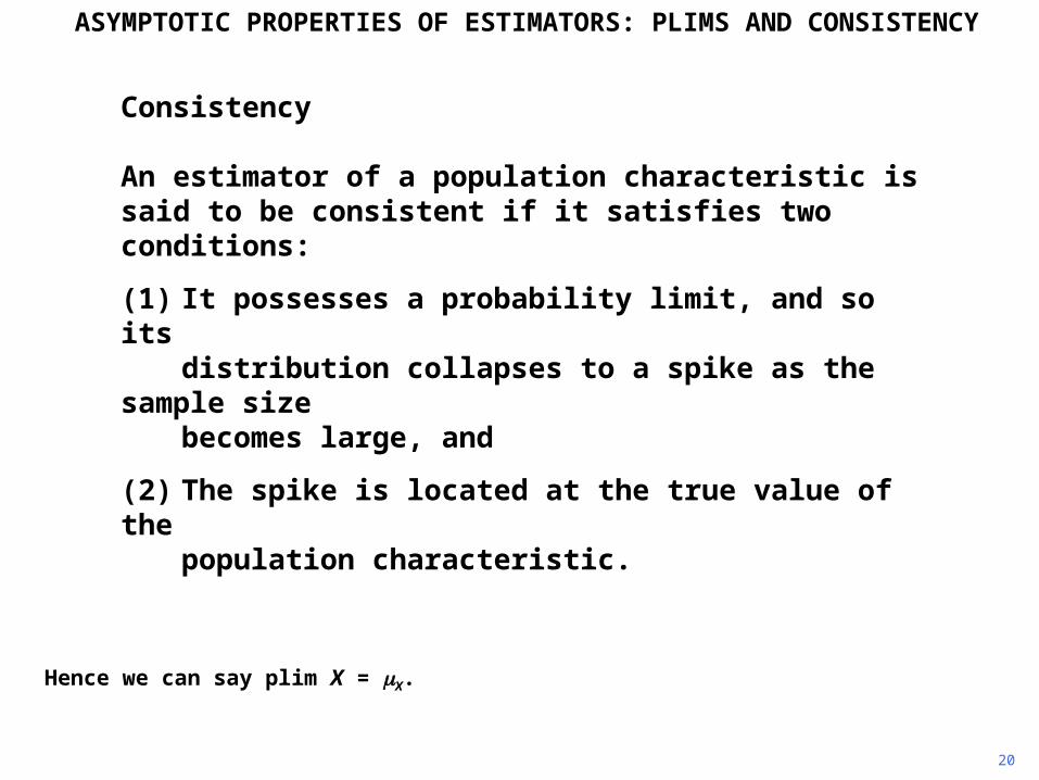
Consistency

An estimator of a population characteristic is said to be consistent if it satisfies two conditions:

(1) It possesses a probability limit, and so itsdistribution collapses to a spike as the sample sizebecomes large, and

(2) The spike is located at the true value of thepopulation characteristic.

Hence we can say plim X = X.

20


21

The sample mean in our example satisfies both conditions and so it is a consistent estimator of X. Most standard estimators in simple applications satisfy the first condition because their variances tend to zero as the sample size becomes large.

50 100 150 200

n = 50000.8

0.4

0.2

0.6



22

The only issue then is whether the distribution collapses to a spike at the true value of the population characteristic. A sufficient condition for consistency is that the estimator should be unbiased and that its variance should tend to zero as n becomes large.

50 100 150 200

n = 50000.8

0.4

0.2

0.6



23

It is easy to see why this is a sufficient condition. If the estimator is unbiased for a finite sample, it must stay unbiased as the sample size becomes large.

50 100 150 200

n = 50000.8

0.4

0.2

0.6



24

Meanwhile, if the variance of its distribution is decreasing, its distribution must collapse to a spike. Since the estimator remains unbiased, this spike must be located at the true value. The sample mean is an example of an estimator that satisfies this sufficient condition.

50 100 150 200

n = 50000.8

0.4

0.2

0.6



25

However the condition is only sufficient, not necessary. It is possible that an estimator may be biased in a finite sample …

n = 20

Z

probability density function of Z


26

… but the bias becomes smaller as the sample size increases

n = 100

n = 20


Z


27

… to the point where the bias disappears altogether as the sample size tends to infinity. Such an estimator is biased for finite samples but nevertheless consistent because its distribution collapses to a spike at the true value.

n = 100

n = 1000

n = 20


Z

n = 100000 ASYMPTOTIC PROPERTIES OF ESTIMATORS: PLIMS AND CONSISTENCY

28

A simple example of an estimator that is biased in finite samples but consistent is shown above. We are supposing that X is a random variable with unknown population mean X and that we wish to estimate X.

.1

1

1

n

iiXn

Z

Consistency


29

The estimator is biased for finite samples because its expected value is nX/(n + 1). But as n tends to infinity, n /(n + 1) tends to 1 and the estimator becomes unbiased.

.1

1

1

n

iiXn

Z

.1 Xnn

ZE

Consistency


30

The variance of the estimator is given by the expression shown. This tends to zero as n tends to infinity. Thus Z is consistent because its distribution collapses to a spike at the true value.

.1

1

1

n

iiXn

Z

.1 Xnn

ZE

2

21)var( X

n

nZ

Consistency


31

Consistency

In practice we deal with finite samples, not infinite ones. So why should we be interested in whether an estimator is consistent?

One reason is that sometimes it is impossible to find an estimator that is unbiased for small samples. If you can find one that is at least consistent, that may be better than having no estimate at all.

A second reason is that often we are unable to say anything at all about the expectation of an estimator. The expected value rules are weak analytical instruments that can be applied in relatively simple contexts.

In particular, the multiplicative rule E{g(X)h(Y)} = E{g(X)} E{h(Y)} applies only when X and Y are independent, and in most situations of interest this will not be the case. By contrast, we have a much more powerful set of rules for plims.


32

Consistency






33

Consistency






34

Consistency






35

Plim rules

Plim rule 1 The plim of the sum of several variables is equal tothe sum of their plims. For example, if you have threerandom variables X, Y, and Z, each possessing a plim,

plim (X + Y + Z) = plim X + plim Y + plim Z

Plim rule 2 If you multiply a random variable possessing a plim bya constant, you multiply its plim by the same constant.If X is a random variable and b is a constant,

plim bX = b plim X

Plim rule 3 The plim of a constant is that constant. For example,if b is a constant,

plim b = b


36

Plim rules




plim bX = b plim X


plim b = b


37

Plim rules




plim bX = b plim X


plim b = b


38

Plim rules

Plim rule 4 The plim of a product is the product of the plims, ifthey exist. For example, if Z = XY, and if X and Y bothpossess plims,

plim Z = (plim X)(plim Y)

Plim rule 5 The plim of a quotient is the quotient of the plims, ifthey exist. For example, if Z = X/Y, and if X and Y bothpossess plims, and plim Y is not equal to zero,

plim Z =plim X

plim Y


39

Plim rules

Plim rule 4 The plim of a product is the product of the plims, ifthey exist. For example, if Z = XY, and if X and Y bothpossess plims,

plim Z = (plim X)(plim Y)

Plim rule 5 The plim of a quotient is the quotient of the plims, ifthey exist. For example, if Z = X/Y, and if X and Y bothpossess plims, and plim Y is not equal to zero,

plim Z =plim X

plim Y


40

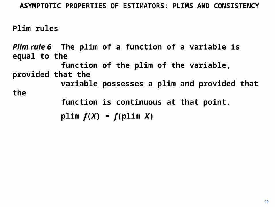
Plim rules

Plim rule 6 The plim of a function of a variable is equal to thefunction of the plim of the variable, provided that thevariable possesses a plim and provided that thefunction is continuous at that point.

plim f(X) = f(plim X)


41

Example use of asymptotic analysis

ZY

To illustrate how the plim rules can lead us to conclusions when the expected value rules do not, consider this example. Suppose that you know that a variable Y is a constant multiple of another variable Z


42


ZY

Z is generated randomly from a fixed distribution with population mean Z and variance 2Z.

is unknown and we wish to estimate it. We have a sample of n observations.


43


ZY

wZX

Y is measured accurately but Z is measured with random error w with population mean zero and constant variance 2

w. Thus in the sample we have observations on X, where X = Z + w, rather than Z.


44


ZY

wZX

One estimator of l (not necessarily the best) is Yi / Xi

wZw

wZ

w

wZ

Z

wZ

Z

X

Y

ii

i

ii

i

ii

i

i

i


45


ZY

wZX

Substituting from the first two equations, the estimator can be rewritten as shown.

wZw

wZ

w

wZ

Z

wZ

Z

X

Y

ii

i

ii

i

ii

i

i

i


46


ZY

wZX

The expression can be simplified as shown. Hence we have decomposed the estimator into the true value, , and an error term. To investigate whether the estimator is biased or unbiased, we need to take the expectation of the error term.

wZw

wZ

w

wZ

Z

wZ

Z

X

Y

ii

i

ii

i

ii

i

i

i


47


ZY

wZX

But we cannot do this. The random quantity appears in both the numerator and the denominator and the expected value rules are too weak to allow us to investigate the expectation analytically.

wZw

wZ

w

wZ

Z

wZ

Z

X

Y

ii

i

ii

i

ii

i

i

i


48


ZY

wZX

However, we know that a sample mean tends to a population mean as the sample size tends to infinity, and so plim w = 0 and plim Z = Z.

wZw

wZ

w

wZ

Z

wZ

Z

X

Y

ii

i

ii

i

ii

i

i

i


49

ZY

wZX

Since the plims of the numerator and the denominator of the error term both exist, we are able to take the plim of the error term. Thus we are able to show that the estimator is consistent, despite the fact that we cannot say anything about its finite sample properties.

00

plim plim plim

plimZi

i

wZw

X

Y



Copyright Christopher Dougherty 2011.

These slideshows may be downloaded by anyone, anywhere for personal use.

Subject to respect for copyright and, where appropriate, attribution, they may be

used as a resource for teaching an econometrics course. There is no need to

refer to the author.

The content of this slideshow comes from Section R.14 of C. Dougherty,

Introduction to Econometrics, fourth edition 2011, Oxford University Press.

Additional (free) resources for both students and instructors may be

downloaded from the OUP Online Resource Centre

http://www.oup.com/uk/orc/bin/9780199567089/.

Individuals studying econometrics on their own and who feel that they might

benefit from participation in a formal course should consider the London School

of Economics summer school course

EC212 Introduction to Econometrics

http://www2.lse.ac.uk/study/summerSchools/summerSchool/Home.aspx

or the University of London International Programmes distance learning course

20 Elements of Econometrics

www.londoninternational.ac.uk/lse.

11.07.25

http://www.oup.com/uk/orc/bin/9780199567089/

http://www2.lse.ac.uk/study/summerSchools/summerSchool/Home.aspx

Documents

Christopher Dougherty EC220 - Introduction to econometrics (review chapter) Slideshow: asymptotic properties of estimators: plims and consistency Original