Choosing the Field of Study in Post-Secondary Education ...ftp.iza.org/dp4127.pdf · Choosing the Field of Study in Post-Secondary Education: Do Expected Earnings Matter? Magali Beffy

IZA DP No. 4127

Choosing the Field of Study in Post-SecondaryEducation: Do Expected Earnings Matter?

Magali BeffyDenis FougèreArnaud Maurel

DI

SC

US

SI

ON

PA

PE

R S

ER

IE

S

Forschungsinstitutzur Zukunft der ArbeitInstitute for the Studyof Labor

April 2009

Choosing the Field of Study in

Post-Secondary Education: Do Expected Earnings Matter?

Magali Beffy CREST-INSEE and IZA

Denis Fougère

CNRS, CREST-INSEE, CEPR and IZA

Arnaud Maurel CREST-ENSAE, PSE and IZA

Discussion Paper No. 4127 April 2009

IZA

P.O. Box 7240 53072 Bonn

Germany

Phone: +49-228-3894-0 Fax: +49-228-3894-180

E-mail: [email protected]

Any opinions expressed here are those of the author(s) and not those of IZA. Research published in this series may include views on policy, but the institute itself takes no institutional policy positions. The Institute for the Study of Labor (IZA) in Bonn is a local and virtual international research center and a place of communication between science, politics and business. IZA is an independent nonprofit organization supported by Deutsche Post Foundation. The center is associated with the University of Bonn and offers a stimulating research environment through its international network, workshops and conferences, data service, project support, research visits and doctoral program. IZA engages in (i) original and internationally competitive research in all fields of labor economics, (ii) development of policy concepts, and (iii) dissemination of research results and concepts to the interested public. IZA Discussion Papers often represent preliminary work and are circulated to encourage discussion. Citation of such a paper should account for its provisional character. A revised version may be available directly from the author.

mailto:[email protected]

IZA Discussion Paper No. 4127 April 2009

ABSTRACT

Choosing the Field of Study in Post-Secondary Education: Do Expected Earnings Matter?*

This paper examines the determinants of the choice of the major when the length of studies is uncertain, by using a framework in which students entering post-secondary education are assumed to anticipate their future earnings. For that purpose, we use French data coming from the 1992 and 1998 Génération surveys collected by the Centre d’Etudes et de Recherches sur l’Emploi et les Qualifications (CEREQ, Marseille). Our econometric approach is based on a semi-structural three-equations model, which is identified thanks to some exclusion restrictions. We exploit in particular exogenous variations in the earnings returns associated with the majors across the business cycle, in order to identify the causal effect of expected earnings on the probability of choosing a given major. Relying on a three-component mixture distribution, we account for correlation between the unobserved individual-specific terms affecting the preferences for the majors, the unobserved individual-specific factors entering the equation determining the length of studies within each major, and that affecting the labor market earnings equation. Following Arcidiacono and Jones (2003), we use the EM algorithm with a sequential maximization step to produce consistent parameter estimates. Simulating for each given major a 10 percent increase in the expected earnings suggests that expected earnings have a statistically significant but quantitatively small impact on the allocation of students across majors. JEL Classification: J24, C35, D84 Keywords: post-secondary education, major choice, returns to education, EM algorithm Corresponding author: Arnaud Maurel ENSAE Bureau E12 - Timbre J120 3, Avenue Pierre Larousse 92245 Malakoff cedex France E-mail: [email protected] * We thank Christian Belzil, Moshe Buchinsky, Nicolas Chopin, Xavier d’Haultfoeuille, Francis Kramarz, Guy Laroque, Robert Miller, Jean-Marc Robin, Gerard J. van den Berg, participants in the IZA Workshop on “Heterogeneity in Micro Econometric Models” (Bonn, June 2007), in the 4th Symposium of the CEPR Network on “Economics of Education and Education Policy in Europe” (Madrid, October 2007), in the 11th IZA European Summer School in Labor Economics (Buch-Ammersee, May 2008), in the 63rd European Meeting of the Econometric Society (Milan, August 2008), in the 2008 EALE Annual Conference (Amsterdam, September 2008), in the 2009 North American Winter Meeting of the Econometric Society (San Francisco, January 2009), and in seminars at CREST-INSEE (Paris, January 2008), Université du Maine (Le Mans, January 2008), Université Paris 1-Sorbonne (Paris, June 2008), and DEPP (Ministry of Education, Paris, December 2008), for very helpful discussions and comments.

mailto:[email protected]

1 IntroductionOver recent years, the French post-secondary education system has been the subject of muchdebate and sharp criticism. In a report for the French Council of Economic Analysis, Aghion andCohen (2004) emphasize the main difficulties that this system, and especially the French univer-sity, have to cope with. Pointing out, among others, the high dropout rate in French universities,they argue that the French post-secondary education system needs urgently to be reformed. Inthis context, it seems in particular crucial to understand students’ educational choices.

In this paper, we focus on the effect of expected labor market income on the choice of thepost-secondary field of study. In particular, we assess the sensitivity of students’ major choices toexpected earnings by estimating a semi-structural model of post-secondary educational choices.More precisely, we try to disentangle the simultaneous effects of, on the one hand, preferencesand abilities, and on the other hand, expected returns, on the choice of major. In the existing ap-plied literature, several papers explicitly consider the impact of expected labor market earningson schooling choices. A first set of papers study these issues by using a rational expectationsframework. In a seminal paper, Willis and Rosen (1979) allow the demand for college educationto depend on expected future earnings.1 Assuming that students form rational (i.e. unbiased)expectations, these authors show that the expected flow of post-education earnings are strong de-terminants of college attendance. Berger (1988) also focuses on the impact of expected earningson the individual demand for post-secondary education: his results show that, when choosingcollege majors, students are more influenced by the expected flow of future earnings than bytheir expected initial earnings.2 Then, following Keane and Wolpin (1997), several econometri-cians have estimated structural dynamic models of schooling decisions (Cameron and Heckman,1998, 2001; Eckstein and Wolpin 1999; Keane and Wolpin, 2001; Belzil and Hansen, 2002;Lee, 2005).3 Their papers assume that students form rational earnings expectations conditionalon schooling decisions, and that the expected earnings affect in turn their educational choices.Recently, Arcidiacono (2004, 2005) has considered sequential models of college attendance, ac-counting both for the demand as well as the supply side of schooling, in which the value ofeach major depends on the corresponding expected flow of earnings. However, in the literaturequoted above, papers by Berger (1988) and Arcidiacono (2004, 2005) are the only ones focusingon the effect of expected earnings on the choice of major and not on the educational level. Ourpaper builds on this literature by assuming that students face an uncertain length of studies whenchoosing their post-secondary major. As we will see further, including uncertainty in terms oflevel of education within each major seems to be necessary to correctly account for the observededucational paths.

A second set of papers examines the validity of the rational expectations assumption in the

1On a related ground, Altonji (1993) estimates a sequential model in which schooling decisions depend onexpected returns to education, without explicitly considering the choice of major.

2Several other articles have shown that there exist some large differences in earnings across majors in the U.S.(see, for instance, James et al., 1989; Loury and Garman, 1995; Brewer, Eide and Ehrenberg, 1999) However, noneof these papers model the choice of the major itself as a function of expected earnings.

3Unlike the preceding papers which rely on partial equilibrium settings, Lee(2005) specifies and estimates ageneral equilibrium model of work, schooling and occupational choices.

2

context of educational choices. More precisely, these papers consider the specification and theestimation of schooling decision models in which the rational expectations assumption is relaxed.In particular, Freeman (1971, 1975) and Manski (1993) have proposed models assuming that in-dividuals have myopic expectations relatively to their potential labor market earnings. Withinsuch a framework, students are assumed to form their wage expectations by observing the earn-ings of comparable individuals who are currently working. According to Manski’s terminology,such expectations are computed “in the manner of practicing econometricians”. More recently,Boudarbat and Montmarquette (2007) examine the effect of expected earnings on the choice ofthe field of studies in Canada; for that purpose, they estimate a mixed multinomial logit modelapplied to the choice of major, using a sample of Canadian university graduates. These authorsalso relax the assumption of rational expectations; assuming myopic expectations, the predictedearnings are computed from the wages of young individuals who have the same education leveland who are currently working.

Our paper contributes to the literature on the effects of expected earnings on schoolingchoices in several ways. First, unlike the previous papers, our approach concentrates on theeffects of expected earnings on the choice of the major, in a framework in which the length ofpost-secondary studies is uncertain to the individual when choosing her major. Stylized factsappear to be consistent with such a framework.4 Another interesting feature of our paper lies inthe fact that we exploit the arguably exogenous variation across the business cycle in the relativereturns to each major in order to identify these elasticity parameters.

Using the parameter estimates of our model, we calculate the elasticities of major choices toexpected earnings by simulating exogenous variations of earnings distribution. These elasticitiesappear to be very low, which means that the choice of a major is mainly driven by non-pecuniaryfactors.

Our study has two main restrictions. First, in the absence of appropriate information al-lowing identification of risk-aversion coefficients, we cannot identify a model incorporating in-dividual attitudes towards risk.5 However, by allowing for heteroskedacticity in the varianceof log-earnings and by imposing a CRRA utility function with a fixed risk aversion parameter,we then estimate an additional specification of our baseline model. Second, we also ignore thepossibility for the student to switch major during her post-secondary studies. Such a switch ispotentially an endogenous event whose treatment would make the model much more compli-cated. However, stylized facts show that this last assumption is sensible for the pooled majorsthat we consider (see Table 8, Appendix A).

The remainder of the paper is organized as follows. Section 2 describes our econometricmodel. The specification of this model and the likelihood function are discussed in Section 3.Section 4 describes the data and presents some preliminary statistics, while Section 5 presentsthe identification strategy and Section 6 contains the estimation and simulation results. Finally,Section 7 summarizes and concludes.

4Indeed, descriptive statistics from the French Panel 1989 database (DEPP, French Ministry of Education) showthat most students complete a final level of education which is different from the level they wanted to reach whenentering college (see Appendix A, Table 9).

5Among recent studies addressing this issue, the reader can consult papers by Belzil and Hansen (2004), Saksand Shore (2005), Brodaty, Gary-Bobo and Prieto (2006).

3

2 The econometric modelAfter graduating from high-school, individuals are assumed to choose their field of post-secondarystudy (major). In this major, they reach some (partly random) level of education. Note that werestrict our analysis to individuals who attend university.6 Once they leave the post-secondaryeducation system, they are supposed to enter the labor market. Thus we consider a sequence ofthree events:

• First stage: when entering college, each student chooses her post-secondary major;

• Second stage: she keeps on studying in the field chosen in the first stage, until she reachesan endogenously determined level of education (dropout, college, BA degree, MA degree,graduate);

• Third stage: she leaves the post-secondary education system and participates in the labormarket.

Following Heckman and Singer (1984), we assume that there are R types of individuals,Πr denoting the proportion of type r in the population of students.7 Individuals are supposed toknow their type which is not observed by the econometrician. Within this framework, unobservedheterogeneity (i.e. unobserved preferences for each major, unobserved schooling ability andunobserved labor market productivity) is type-specific.

2.1 Stage 1: Choice of the majorAfter graduating from high-school (and getting the final high-school diploma, called “Baccalau-réat” in France), the individual who decides to continue studying must choose the college major,hereafter indexed by j∗.8 We assume that this choice is made among a set of M majors. Further-more, we assume that the chosen field j∗ depends on the individual’s expectations concerningboth the education level that she will achieve within this major (stage 2), and her future labormarket earnings, which are assumed to depend on her educational level (stage 3). An importantunderlying assumption is that future earnings as well as the highest level of education reached infield j∗ are partly uncertain.9

For a student of type r, let us denote by V rj the value function associated with the choice of

field j (j = 1, . . . ,M). This value function is assumed to be composed of two additive elements,

6The argument justifying our choice to focus on individuals attending university is detailed in the section devotedto the data.

7Examples of econometric models of schooling decisions relying on a similar assumption can be found in Keaneand Wolpin (1997, 2001), Eckstein and Wolpin (1999), Cameron and Heckman (1998, 2001), Belzil and Hansen(2002, 2004), Arcidiacono (2004, 2005) and Lee (2005).

8We omit the individual subscript for the sake of simplicity.9We suppose that each individual has an idiosyncratic propensity to achieve a high level of education. This

propensity is partly affected by random factors, such as her own health status and unexpected changes in her familyenvironment. These factors are ex ante unknown by the individual when choosing her major, and then revealedwhen attending university.

4

respectively denoted by v0j and vr1j . The first term vr

0j represents the intrinsic value (i.e. theconsumption value) of the major, while vr

1j may be considered as the investment value of a post-secondary education in field j. It is a function of the sum of the expected future average (monthly)labor market earnings which are associated with the L + 1 educational levels that can be reachedwithin field j, each of these expected values being weighted by the probability Pr(K = k | J =j) to reach the k-th educational level (k = 0, ..., L) within field j (j = 1, ...,M). Here k = Ldenotes the highest educational level that can be reached within major j, and k = 0 correspondsto the case where the student drops out from the major before terminating the first year of college.Then, for a student of type r, the value V r

j of major j can be written as :

V rj = vr

0j + vr1j, for j = 1, ...M (1)

wherevr

1j = α∑

k∈{0,1,...,L}

Pr(K = k | r, J = j).E(V r

e(j,k) | r, J = j, K = k)

E(V r

e(j,k) | r, J = j, K = k)

denoting the expected flow of earnings associated with education

(j, k), for a student of type r, and α being an unknown sensitivity parameter to be estimated.10

The subcomponent vr0j can be interpreted as the non-pecuniary value of field j for a student

of type r. It may correspond to the “social gratification” brought by studying in major j or to theindividual’s taste for this major. We assume that vr

0j is a linear function of a set of observableindividual covariates that affect the attractiveness of field j (e.g. gender, place of birth, parents’nationality and profession, past educational history of the student, including the cumulated delaywhen entering secondary school). It is also depending on a type-specific intercept αr

(1,j) and on arandom term uj independent of αr

(1,j). Consequently, vr0j is specified as

vr0j = αr

(1,j) + X ′1β

j1 + uj

where βj1 is a parameter vector associated with X1 and specific to field j. The individual chooses

the education field j∗ that corresponds to the highest value function:

j∗ = arg maxj∈{1,...,M}

V rj

2.2 Stage 2: Determination of the length of studiesOnce a student of type r has chosen her major j∗, she studies until she reaches a level k∗j ofeducation within field j. We assume that this level k∗j is an element of a set of L + 1 possiblelevels corresponding to the different degrees which may be obtained in each major; k = 0corresponds to a dropout, which occurs when a student leaves university during the first yearof college (without any post-secondary degree), k = 1 refers to the degree called “DEUG” inFrance which is generally obtained after two years of college, k = 2 corresponds to the BA

10The functional form of probabilities Pr(K = k | r, J = j) is specified in the next section.

5

degree (called “Licence” in France), k = 3 corresponds to the MA degree (“Maîtrise”) andk = L = 4 refers to the Graduate level.

The length of studies k∗j within major j is supposed to be determined by the individualpropensity kj to succeed in long post-secondary studies within this major.11 More precisely,we assume that the length of studies k∗j is generated by the following latent model:

k∗j =

0 if kr

j ≤ s1

1 if s1 < krj ≤ s2

...L if sL < kr

j

where {s1, . . . , sL} are latent (unknown) thresholds that correspond to the minimum ability levelsrequired to obtain the different degrees. The latent propensity kr

j is assumed to depend linearly onobservable covariates X2 (such as gender, nationality, parents’ profession, etc..). It also dependson a type-specific intercept αr

2 and on an independent term v which is unknown ex ante by thestudent when she decides to enter college. Thus the propensity kr

j is defined as:

krj = αr

2 + X ′2,jβ2 + v (2)

where αr2 and β2 are unknown parameters to be estimated. In this expression, X2,j is a vector

of exogenous regressors including individual characteristics but also covariates that are specificto the major j. Namely, we allow the average proportion of college students in the same majorand in the same university to affect the length of studies.12 In the absence of variables plausiblyaffecting the choice of major but not the length of studies, we choose to exclude major-specificdummies in X2,j since the related coefficients would only be identified through nonlinearities.

Note that, in our framework, the length of studies is not the number of years spent effectivelyin post-secondary education, but the terminal level of education that is reached by the student,whatever the time spent at the university. We should also remark that we do not account forselection of applicants by the university administration at the entry of college: this seems to be aquite sensible assumption for the French university system.

2.3 Stage 3: Labor market earningsHaving obtained the educational level (degree) k∗j in major j∗, the student then enters the la-bor market. We assume that the labor market is an absorbing state: individuals do not resumestudies after entering the labor force. When making her post-secondary schooling decision inthe first stage, the individual is assumed to anticipate the impact of the major and of the lengthof the studies on her future labor market earnings. In order to take both employment and non-employment spells into account, we refer to average earnings as the sum of wages weighted

11This framework is consistent with an ordered probit model.12This variable is calculated using information coming from the SISE database provided by the French Ministry

of Education.

6

by employment spell durations, and unemployment benefits13 weighted by unemployment spelldurations. Hence, the logarithm of the average monthly earnings received over a period of lengthTobs (in months) by a worker with education (j, k) and of type r, is given by :

ln wr

jk = ln

∑Ne

s=1 ws,jkles +

∑Nu

s′=1 bs′,jklus′

Tobs

(3)

with

Tobs =Ne∑s=1

les +Nu∑

s′=1

lus′

where Ne (respectively, Nu) is the number of observed employment (unemployment) spells inthe individual labor market history, ws,jk is the monthly wage in the s-th employment spell, les(respectively, bs′,jk is the monthly unemployment benefit in the s′-th unemployment spell, lus ) aredurations of the s-th employment (respectively, unemployment) spell, and Tobs is the total lengthof the observed labor market history of the individual. By definition, we set:

V re(j,k) = ln w

r

jk (4)

Thereafter, we focus only on this aggregate notion of labor market earnings, without mod-eling separately wages and individual probabilities of employment (and nonemployment). Thisappears to be consistent with the students’ behavior when they take their post-secondary school-ing decisions: most individuals anticipate future labor market conditions as a whole, withoutseparately taking into account the effects of their educational choices on wages and on employ-ment probabilities.

Labor market earnings depend on the post-secondary educational field and level, namely onthe pair (j∗, k∗j ). Note that our framework accounts for the earnings gaps, not only across school-ing levels (within a given field of study), but also across fields of study (for a given educationallevel, or degree). Earnings are also supposed to be a function of exogenous and predeterminedindividual characteristics. For a student of type r, the average log-earnings equation is assumedto be given by:

ln wr

jk = αr3 + X

′

3(j,k)β3 + ε (5)

where X3(j,k) is a vector of observed characteristics that may affect labor market earnings, in-cluding post-secondary education, αr

3 represents the type-specific intercept, and ε denotes anindependent random factor that affects the individual’s earnings.

3 Model specificationLet us recall that the type-specific intercepts are mass points of a discrete distribution with prob-abilities (Π1, ..., ΠR) verifying

∑Rr=1 Πr = 1, and that the residuals of the three equations are

stochastically independent of these type-specific intercepts.14

13Unemployment benefits are assumed to be equal to a constant times the former wage received when employed.This constant is taken equal to 0.7 as often done in the literature.

14Some covariates introduced in the equations may not be independent of the individual’s type. It applies espe-cially to the high school graduation track, which may be in particular related to unobserved preferences for each

7

3.1 Stochastic assumptionsResiduals are supposed to be normally distributed. We assume that the random vector (u1, . . . , uM)affecting the choice equation, and the residuals v and ε entering the two other equations are inde-pendently distributed.15 Consequently, the whole vector of residuals16 is assumed to be distrib-uted as:

vu2 − u1

u3 − u1

...uM − u1

ε

∼ N (0, Σ)

where Σ is the (M + 1) × (M + 1) covariance matrix of the model residuals, with Σ[1, 1] = 1and Σ[2, 2] = 1 for identifiability reasons. Given the constraints we impose on correlations, thecovariance matrix is:

Σ =

1 ... ... ... ... ...0 1 ... ... ... ...0 Σ32 Σ33 ... ... ...... ... ... ... ... ...0 ΣM2 ... ... ΣMM ...0 0 ... ... 0 Σ(M+1),(M+1)

(6)

The particular order of the residuals in this vector enables us both to use Cholesky decompositionand to verify our constraints. Thus, if Γ denotes the Cholesky factor for the covariance matrix Σ,we have:

Σ = Γ.Γ′ (7)

where

Γ =

1 0 0 ... ... 00 1 0 0 ... 00 α32 exp(d1) 0 ... 0... ... ... ... ... ....0 0 ... ... 0 exp(dM−1)

(8)

Note that we impose the positivity of the diagonal terms of matrix Γ. Hence, the Choleskydecomposition of Σ is unique.

major. Nevertheless, conditioning the type probabilities on the high school graduation track did not change signifi-cantly our results.

15Correlated unobserved heterogeneity across equations is captured by type-specific random intercepts(αr

(1,j))j=1,...,M , αr2, and αr

3.16Only differences in utility levels matter in random utility models.

8

3.2 The likelihood functionUnder our stochastic assumptions, the contribution to the likelihood function of an individualof type r who chooses the major j∗, who reaches the educational level (k∗j ), and who gets theaverage labor market log-earnings ln w

r

jk is:

l(j∗, k∗j∗ , ln wr

jk|r) = Pr

[ ⋂j′ 6=j∗

(uj′ − uj∗ ≤ fr (j∗)− fr (j′))

]× g(ε)

×Pr[sk∗

j∗− hr < v ≤ sk∗

j∗+1 − hr

](9)

wherehr = αr

2 + X ′2,jβ2

fr (j) = αr(1,j) + X ′

1βj1 + α

M∑k=0

X3(j,k)β3 ×[Φ(sk+1 − hr

)− Φ

(sk − hr

)]

g(ε) =1√

Σ[M + 1, M + 1]× ϕ

(ε√

Σ[M + 1, M + 1]

)with

ε = ln wr

j,k − αr3 −X3(j,k)β3

andPr[sk − hr < v ≤ sk+1 − hr

]= Φ

(sk+1 − hr

)− Φ

(sk − hr

)ϕ and Φ being respectively the density and cumulative density functions of the standard normaldistribution N (0, 1).Note that the first stage of the econometric model corresponds to the esti-mation of a multinomial probit model. Within this framework, the choice probabilities Pr(j|r)do not have a closed-form expression.17 As it is detailed in the following section devoted to data,estimations are based on J = 3 aggregated majors. Thus, in stage 1, each choice probability isexpressed as a double integral which can be evaluated using usual integration procedures (suchas quadrature methods), without the need to rely on a GHK probit simulator.

Unconditional on the type, the contribution to the likelihood function of a student whochooses the field j∗, who reaches the educational level k∗j∗ and who gets the average labor marketlog-earnings ln wj∗,k∗

j∗follows a finite mixture distribution:

l(j∗, k∗j∗ , ln wj∗,k∗j∗

) =R∑

r=1

Πrl(j∗, k∗j∗ , ln w

r

j∗,k∗j∗|r) (10)

where l(j∗, k∗j∗ , ln wr

j∗,k∗j∗|r) denotes the individual contribution to the likelihood given the type

r.17Each choice probability is a J − 1 dimensional integral which must be evaluated numerically.

9

3.3 EstimationIn order to present our estimation strategy, let us introduce some further notations: θF denotesthe whole parameters of the choice equation, θL those of the equation for the length of studies,and finally θW those of the wage equation. These vectors do not include type-specific intercepts.

As it is usual for a finite mixture of gaussian distributions, we rely on the Expectation-Maximization (EM) algorithm (Dempster, Laird and Rubin, 1977) to estimate our model. Thisalgorithm works by iterating the two following steps until the stability of the log-likelihood func-tion is reached.

At each iteration n of this algorithm, we use the values(θ

(n)F , θ

(n)L , θ

(n)W

)of the parameter

vector, the values (π(n)r )r=1...R of the mixture distribution and the values (α

(n)r )(r) of the type-

specific intercepts, which are all obtained from the previous iteration of the algorithm. Moreprecisely, the two steps are the following:

B E-step

For each type r = 1, ..., R, and for each individual i, the posterior probability for theindividual i to be of type r is:

Pr (Ti = r|j∗i , k∗i , wi, Xi) =π

(n)r Pr(j∗i , k

∗i , wi|Ti = r, Xi)∑R

r=1 π(n)r Pr(j∗i , k

∗i , wi|Ti = r, Xi)

where Ti is the random variable representing the individual type. In the following, π(n)i,r de-

note these posterior probabilities. Then, we compute the expected completed log-likelihood:

N∑i=1

R∑r=1

π(n)i,r ln l (j∗i , k

∗i , wi|Ti = r, (Πr)r, (αr)r, θF , θL, θW ) (11)

B M-step

We maximize the expected completed log-likelihood function in terms of ((Πr)r, (αr)r, θF , θL, θW ).

This maximization can be done in two successive steps.

First we update π(n)k such as:

π(n+1)r =

∑Ni=1 π

(n)ir∑R

l=1

∑Ni=1 π

(n)il

(12)

Then, due to the partial separability of the conditional completed log-likelihood function(Arcidiacono and Jones, 2003), we get three sequential optimization problems since resid-

10

uals are assumed to be independent across the three equations. Henceforth:

N∑i=1

R∑r=1

π(n)i,r ln l (fi, li, wi|Ti = r, (Πr)r, (αr)r, θF , θL, θW )

=N∑

i=1

R∑r=1

π(n)i,r ln l

(wi|Ti = r, (Πr)r, (α

Wr )r, θW

)+

N∑i=1

R∑r=1

π(n)i,r ln l

(li|Ti = r, (Πr)r, (α

Wr )r, (α

Lr )r, θW , θL

)+

N∑i=1

R∑r=1

π(n)i,r ln l

(fi|Ti = r, (Πr)r, (α

Wr )r, (α

Lr )r, (α

Fr )r, θW , θL, θF

)It implies that first, we maximize the log-wage equation. Given the estimates of this equa-tion, we estimate the parameters of the equation for the length of studies. Finally, given theprevious estimates, we maximize the choice equation. Although this procedure does notyield full information maximum likelihood estimates, Arcidiacono and Jones (2003) showthat this method produces consistent estimates of the parameters, with large computationalsavings.

In order to get standard errors estimates, we rely on a parametric bootstrap procedure,instead of a non parametric one, since this last method is unstable when applied to the EMalgorithm. The parametric bootstrap consists first in obtaining reliable parameter estimatesdenoted θ. We get θ by replicating the previously described EM algorithm with differentrandom initial values for the parameters. The iteration process is necessary to ensure theconvergence to a global maximum. Then, given X and θ, we draw H vectors of theendogenous variables

(jhi , kh

i , whi

)h=1...H

. For each newly generated data set, we estimateθ∗h. Final parameters and standard errors estimates are calculated as:

θ∗ =1

H

H∑h=1

θ∗h (13)

σθ∗ =1

H − 1

H∑h=1

(θ∗h − θ∗)2 (14)

4 DataThe model presented above is estimated using French data coming from the “Génération 92”and “Génération 98” surveys, which are collected by the Centre d’Etudes et de Recherches surl’Emploi et les Qualifications (CEREQ, Marseille).18 The “Génération 92” survey consists of

18These data have been previously used by Brodaty, Gary-Bobo and Prieto (2006), who estimate a structuralmodel of individual educational investments in presence of students’ attitudes toward risk.

11

a large sample of 26,359 individuals who left the French educational system in 1992 and wereinterviewed five years later, in 1997. In the original sample, education levels range from thelowest to the highest one, respectively referred to as “Level VI” and “Level I” in the Frenchnomenclature. This database has the main advantage to contain information on both educationaland labor market histories (over the first five years following the exit from the educational sys-tem). Furthermore, the survey provides a set of individual covariates which are used as controlsin our estimation procedure such as gender, place of birth, nationality, parents’ profession, andresidence when leaving the educational system. Most of the individual covariates observed inthe “Génération 92” survey are also provided by the “Génération 98” survey, which consists ofa sample of 22,021 individuals who left the French educational system six years later, in 1998,and were interviewed in 2003.19 In this paper, we exploit the pooled dataset which containsinformation on a total of 48,380 individuals entering the labor market either in 1992 or in 1998.

Our subsample of interest is constituted of respondents to these surveys and who have at leastpassed the national high school final examination. It is then restricted to 27,389 individuals. Fur-thermore, within this selected sample, we restrict our analysis to the individuals having attendeduniversity, except medicine faculties and IUT (“Institut Universitaire de Technologie”, which aretwo-year vocational colleges). This sample selection was made in order to keep an homogeneousset of post-secondary tracks, both in terms of selection and possible length of studies. Missingcovariates values finally leaves us with a sample of 7,346 individuals.20

Post-secondary studies are aggregated into three broad fields: “Sciences”, “Humanities andSocial Sciences” (including art studies) and “Law, Economics and Management”. We then con-sider five different educational levels (i.e. degrees) that may be reached within each major. Theyare respectively denoted by “dropout” (less than two years of college), “two years of college”,“BA degree” (“Licence” in French), “MA degree” (“Maîtrise”) and “Graduate” (more than fouryears after High School). Tables 1 and 2 below provide basic descriptive statistics for the selectedsubsample. Table 7 (reported in Appendix A) provides a descriptive outlook for the determinantsof post-secondary schooling choices in France.

We first focus on the choice of the major. Table 7 shows that this choice is related withgender, the age in 6th grade,21 and parents’ profession.

Noteworthy, male students are more likely to attend majors in Sciences (39.40% among malevs. 16.42% among females) while female students are more likely to attend majors in Humanitiesand Social Sciences (29.32% among males vs. 48.93% among females). The student’s age in 6th

grade and the chosen field are highly correlated: individuals who were above the “normal” agein 6th grade are less likely to attend a major in Science, while they are more likely to attend amajor in Law, Economics and Management.

19Although a longer observation window is available for each Génération dataset, the average log-earnings arecomputed using only the observations from 1992 to 1995 for Génération 1992 (resp. 1998 to 2001 for Génération1998). In particular, restricting to a 4-years window allow us to limit the number of individuals that have to bedropped because of missing earnings values, in addition to the fact that it allows us to work with two periods ofvirtually opposed economic conditions and helps identifying the earnings elasticities of major choices.

20In order to prevent our estimates to be driven by outliers, we also drop individuals with average log-earningsbelow the 2.5 percentile (respectively above the 97.5 percentile) of the log-earnings distribution.

21This variable can be seen as a proxy for the individual schooling ability.

12

Parental characteristics also seem to play in important role on the choice of the major. Thehigher the parents’ social category, the higher the probability to study sciences. For instance,individuals whose father is a blue-collar worker are more likely to attend a major in Human andSocial Sciences, and less likely to attend a major in Sciences.22 Table 7 also shows a strongcorrelation between the chosen field and the length of studies. Only one quarter of graduatescomplete their degree in Humanities and Social Sciences. Unlike graduates, half of dropoutsduring the first two years of college studied Humanities.

Finally, the higher the educational level, the larger the mean of log-earnings (see Table 3 re-ported below): graduates earn 1.7 times more than dropouts. There are significant differences inaverage earnings associated with the different majors: sciences ranks first, followed by law, eco-nomics and management, and finally humanities and social sciences. The discrepancy betweenmajors is greater in 1998 than in 1992. Sciences and law, economics and management benefitedfrom the macroeconomic expansion that occurred in the late 90’s.

Table 1: Descriptive statistics: majors and levels of post-secondary education

Number PercentMajorSciences 2,106 28.67Humanities and Social Sciences 2,761 37.59Law, Economics and Management 2,479 33.75Post-secondary education levelDropout 1,762 23.99Two years of college 732 9.97Licence (BA degree) 1,400 19.06Maîtrise (MA degree) 1,486 20.23Post Maîtrise (Graduates) 1,966 26.76

Source: Surveys Générations 1992 and 1998 (CEREQ, Marseille)

22Mother’s profession is associated with the field of study in a similar way.

13

Table 2: Descriptive statistics: covariates

Number PercentYear of entry into the labor market1992 3,436 46.771998 3,910 53.23GenderMale 3,197 43.52Female 4,149 56.48Born abroadNo 7,164 97.52Yes 182 2.48Age in 6th grade≤ 10 858 11.6811 6,109 83.16≥ 12 379 5.16Secondary schooling trackHumanities 1,712 23.31Economics and Social Sciences 1,733 23.59Sciences 2,523 34.35Vocational or Technological 1,378 18.76Father’s profession (at the survey date)Farmer or tradesman 1131 15.40Executive 2213 30.13Intermediate occupation 898 12.22White-Collar 1468 19.98Blue-collar 1237 16.84Out-of-the labor force 399 5.43Mother’s profession (at the survey date)Farmer or tradesman 527 7.17Executive 1226 16.69Intermediate occupation 508 6.92White-Collar 3269 44.50Blue-collar 508 6.92Out-of-the labor force 1308 17.81


14

Table 3: Average monthly earnings (1992 French Francs) according to the length and the field ofstudies

Field Length Average earningsPooled surveys

Dropout 4,920Two years of college 5,983Licence (BA degree) 6,181Maitrise (MA degree) 6,739Post Maitrise (Graduates) 8,414

Sciences 7,277Humanities and Social Sciences 5,942Law, Economics and Management 6,666Survey Génération 1992


Sciences 6,833Humanities and Social Sciences 6,088Law, Economics and Management 6,318Survey Génération 1998


Sciences 7,758Humanities and Social Sciences 5,835Law, Economics and Management 6,976


5 Identification strategyFor identifiability reasons, we impose usual restrictions on the type-specific heterogeneity termsof equations 1 and 2. Namely, in the multinomial probit model corresponding to the choiceequation, we set αr

(1,1) = 0,∀r ∈ {1, . . . , R}, and, in the ordered probit model corresponding to

15

the second equation, α12 = 0.

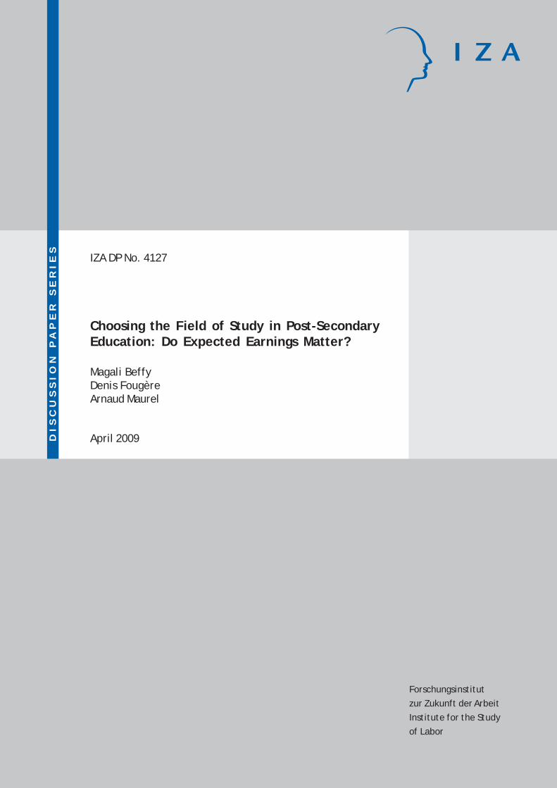
In order to identify our model, and in particular the effect of expected earnings on the prob-ability to choose a major, without relying on distributional assumptions, we exploit variations inthe relative earnings returns induced by the business cycle. In other terms, we take into accountthe fact that these relative returns depend on the year of entry into the labor market.23 Descriptivestatistics reported in Table 3 show that the relative returns to the majors changed significantly be-tween 1992 and 1998: these years correspond respectively to a recession and to an expansion inthe French business cycle.24 Namely, after controlling for the change in the distribution of educa-tional levels between 1992 and 1998 as well as for inflation, we find a relative increase of 13.5%(respectively, 10.4%) in the average earnings associated with majors in sciences (respectively, inlaw, economics and management) between the two periods, while the average earnings associ-ated with majors in humanities and social sciences decreased by 4.2% over the same period.25

Besides, it seems reasonable to assume that the date of entry into the labor market has no directinfluence on the choice of the major, in other words that, other observable things being equal,preferences for the majors were stable during this period.26 In order to identify the elasticity ofthe choice of the major with respect to expected earnings, we exploit the fact that the returns tothe different majors are unequally affected by the business cycle.27 Hence, we introduce into theearnings equation interaction terms between the chosen major and an entry year dummy. Thisdummy variable is equal to zero if the individual enters the labor market in 1992, and to unityotherwise (namely, if she enters the labor market six years later in 1998). Its interaction withthe chosen major is assumed to affect only the earnings and not the two other outcomes. Thisexclusion restriction (over)identifies the parameter α associated with the expected returns in thechoice equation without imposing a distributional assumption on the error terms. Besides, thecovariates indicating the father’s and mother’s professions (respectively in 1992 and 1998), theage of the student in 6th grade, and the high-school major are included in the list of regressorsaffecting the choice of the major and the determination of the length of studies, but they areexcluded from the earnings equation. Similarly to Arcidiacono (2005, section 4), these exclu-sion restrictions, in addition to the assumed functional forms, allow to identify the unobservedheterogeneity types. These covariates may be correlated with the individual’s preferences and

23Berger (1988) also relies on exogenous variations in the wage returns to each major according to the date ofentry into the labor market in order to identify the effect of expected earnings on college major choice. Unlike ours,his framework does not take into account the determination of the length of studies. Besides, his results rely on theIndependence from Irrelevant Alternative assumption for the choice of the major which is unlikely to hold in such acontext.

24See Figure 1 in Appendix A.25These relative variations between 1992 and 1998 are obtained by computing for each major the average of mean

monthly earnings conditional on each educational level, weighted by the frequency of each level.26In particular, we should remark that no reform concerning post-secondary education was implemented in France

between 1992 and 1998. The progressive application of the Bologna process to the French post-secondary educa-tional system began in 1999. Thus it should not affect the choice decisions of the individuals in our sample who hadalready entered the labor market at that time.

27On a related ground, in a recent paper examining the career effects of graduating in a recession, Oreopoulos etal. (2008) show that Canadian college graduates are unequally affected by the recession according to their major ofstudy.

16

ability, represented respectively by αr(1,j) and αr

2. Finally, considering that overcrowding mayaffect educational attainment, we assume that the proportion of college students who attend thesame major in the same university than the individual may influence the length of her studies.

6 ResultsTables 12 and 13 (see Appendix B) report the parameter estimates of the equations generatingthe major choice.

Students whose mother is a white-collar choose less frequently majors in Humanities andSocial Sciences, compared to Sciences, than students whose mother is an executive. Noteworthy,students whose mother is a farmer, a tradeswoman or a white-collar worker, or whose occupiesan intermediate profession, also choose less frequently majors in Law, Economics and Manage-ment compared to Sciences. In all other cases, parental, and in particular father’s profession hasgenerally no effect on the major choice.

The nationality of the student’s parents has a significant and quantitatively large impact onthe choice of a major in Law, Economics and Management as well as in Humanities and SocialSciences, compared to Sciences. Besides, students born abroad are significantly less likely tostudy law, economics or management. Noteworthy, female students are very significantly lesslikely to study sciences. As expected, students who obtained a Baccalauréat in sciences aresignificantly more likely to choose a post-secondary major in sciences. Students who were olderthan expected (i.e. 12 years old or above) at the entry into junior high school (sixth grade) chooseless frequently a major in sciences. Finally, the expected returns in a given post-secondary majorhas a statistically significant but rather small effect on the choice of the major (see the value forthe estimate of the parameter α in Table 12).

Most covariates have a significant impact on the length of post-secondary studies (see Table14). For instance, students whose parents are white-collar or blue-collar workers leave the post-secondary educational system at a lower level. Students whose both parents are French reachgenerally a higher level of post-secondary education. Students who were younger than expected(i.e. 10 years old or below) at the entry into junior high-school reach a higher level of education.Those who obtained their Baccalauréat in sciences are also more likely to reach a higher level ofpost-secondary education. When the proportion of college students who attend the same majorin the same university increases, which implies that the proportion of students preparing a BA orMA degree is lower in this major and in this university, the individual probability of reaching ahigh level of education (B.A. and above) in this major is lower, other things being equal. Thismay result from the selection imposed by the university after the end of college (i.e. at the entryin the third year of post-secondary schooling in the major), or from peers effects; this secondinterpretation is the one set forth by Arcidiacono (2004, 2005). Finally, women are less likely topursue long studies. This is a common result in France: nowadays, on average, French womenare more educated than men, but graduated men are more numerous than women.

Table 15 gives the parameter estimates of the (log-)earnings equation. On average, earningsare lower for females and they are higher in the region Ile-de-France (including Paris). Mean(log-)earnings increase with the length of studies in post-secondary education. However, this in-

17

crease is lower above the BA degree in humanities and social sciences. Noteworthy, the marginalreturns to each additional year of post secondary education are also lower, up to graduate level,for the individuals entering the labor market in 1998 than for those leaving university six yearsbefore. Besides, consistently with the fact that the individuals entering the French labor force in1998 benefit from positive economic conditions (as compared to those entering the labor mar-ket in 1992), mean (log-)earnings are substantially higher for those leaving university in 1998.Finally, while controlling for selection on observables and unobservables renders statistically in-significant the returns to the majors for the individuals leaving university in 1992, those enteringthe labor market in 1998 after graduating in humanities and social sciences experience negativerelative returns.

Tables 16 and 17 report the parameter estimates of the distribution of unobserved individ-ual heterogeneity terms. The first group of individuals represents 38 percent of the populationof students. Individuals in this group are characterized by the lowest unobserved type-specificpreference for studying sciences as well as the highest highest type-specific earnings interceptα3. The second group represents approximatively 34 percent of the population of students. Indi-viduals in this group are characterized by the lowest type-specific preference α(1.3) for studies inlaw, economics and management. They also have the lowest type-specific propensity (or ability)α2 to undertake long post-secondary studies. Finally, the third group represents about 28 percentof the population; it is both characterized by the lowest type-specific earnings intercept term α3

and the highest propensity to pursue long post-secondary studies. Table 18 reports the estimatedproportions of students in each major, at each level of post-secondary education, according toeach type, while Table 19 reports the estimated means and standard errors of log-earning distrib-utions by type. These tables are obtained by attributing to each observed individual the type thatmaximizes her posterior type probability.

The model fit is quite good. Table 4 shows that the model slightly overestimates (resp. under-estimates) the proportion of students in humanities and social sciences (resp. in law, economicsand management).

To get a more precise view of the effect of expected earnings on the choice of the post-secondary major, we run simulation exercises that consider a 10% increase or decrease in theexpected earnings associated with a given major (see Tables 4 to 6 below).28

In general, the impacts are quantitatively small even though they are statistically significant.The lowest impacts concern the majors in sciences. A 10% increase in the expected earningsassociated with majors in sciences leads to an increase of 0.25 percentage points in the proportionof students in this major. This increase is mainly compensated by a decrease of 0.19 percentagepoints in the proportion of students in humanities and social sciences (see Table 4). A 10%decrease in the expected earnings associated with majors in sciences results in almost symmetricvariations in allocations across majors.

Impacts resulting from a 10% increase or decrease in the expected earnings associated withmajors in humanities and social sciences are substantially higher although still quantitativelysmall (see Table 5). For instance, a 10% increase in the expected earnings associated with a post-

28Simulating both types of variation enables us to see whether the impacts on allocations across majors aresymmetric or not.

18

secondary in these majors results in an increase of about 0.53 percentage points in the proportionof students in these majors, this increase being mainly compensated by a decrease of about 0.34percentage points in the proportion of students in law, economics and management and to a lesserextent by a 0.19 points decrease in the proportion of students in sciences. Once again, a 10%decrease in expected earnings has almost symmetric impacts on allocations.

Finally, a 10% increase in the expected earnings associated with a post-secondary educationin law, economics and management majors result in an increase of 0.4 percentage points in theproportion of students in these majors, this increase being mainly compensated by a decrease of0.34 percentage points in the proportion of students in humanities and social sciences (see Table6). The effects are still symmetric for a 10% decrease in the expected earnings associated withthis major.29

The preceding simulation exercises allow us to compute the sample earnings elasticities ofmajor choice, which present the advantage of being easily interpreted. Namely, simulating a10% increase in the expected earnings for each major yields low elasticities of respectively 0.09for sciences, 0.14 for humanities and social sciences, and finally 0.12 for law, economics andmanagement.

The results discussed above were obtained relying on the econometric framework detailedin Section 3, which in particular does not account for log-earnings heteroskedasticity. In orderto address the fact that major choices may also be driven by major and level-specific earningsdispersions, we also run additional estimations relying on an extension of our model accountingfor heteroskedasticity and risk aversion. Namely, we impose an exponential parametric form ofheteroskedasticity, allowing the variance of log-earnings to depend both on the major and on thelevel of education. Besides, we assume that individuals value the major and the level-specificearnings through a CRRA von Neumann-Morgenstern utility function, with a risk aversion pa-rameter taken equal to ρ = 1.1. This means that the mathematical expectations appearing in theexpression of the terms vr

1j for j = 1, ...M (see equation 1), become:

1

1− ρe(1−ρ)µr

j,k+(1−ρ)2σ2

j,k2

where µrj,k and σ2

j,k denote the mean and the variance of log-earnings, respectively. This alterna-tive specification yield fairly similar earnings elasticities of major choice (see Appendix C). Theeffects of expected earnings on major choice are still significant and quantitatively small, withpoint estimates of the same magnitude.

29Given that the model we estimate a priori yields non linear effects of expected earnings on the probability tochoose each major, we also simulated 20% increases in the expected earnings associated with each field of study.The resulting effects are about twice (namely 1.9) larger. We therefore provide the earnings elasticities of majorchoice relying only on the first set of simulations.

19

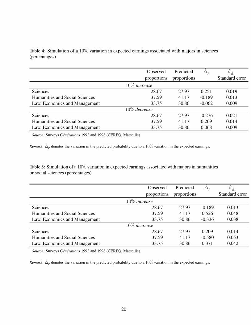
Table 4: Simulation of a 10% variation in expected earnings associated with majors in sciences(percentages)

Observed Predicted ∆p σ∆p

proportions proportions Standard error10% increase

Sciences 28.67 27.97 0.251 0.019Humanities and Social Sciences 37.59 41.17 -0.189 0.013Law, Economics and Management 33.75 30.86 -0.062 0.009

10% decreaseSciences 28.67 27.97 -0.276 0.021Humanities and Social Sciences 37.59 41.17 0.209 0.014Law, Economics and Management 33.75 30.86 0.068 0.009Source: Surveys Générations 1992 and 1998 (CEREQ, Marseille)

Remark: ∆p denotes the variation in the predicted probability due to a 10% variation in the expected earnings.

Table 5: Simulation of a 10% variation in expected earnings associated with majors in humanitiesor social sciences (percentages)



Sciences 28.67 27.97 -0.189 0.013Humanities and Social Sciences 37.59 41.17 0.526 0.048Law, Economics and Management 33.75 30.86 -0.336 0.038

10% decreaseSciences 28.67 27.97 0.209 0.014Humanities and Social Sciences 37.59 41.17 -0.580 0.053Law, Economics and Management 33.75 30.86 0.371 0.042Source: Surveys Générations 1992 and 1998 (CEREQ, Marseille).


20

Table 6: Simulation of a 10% variation in expected earnings associated with majors in law,economics or management (percentages)



Sciences 28.67 27.97 -0.062 0.009Humanities and Social Sciences 37.59 41.17 -0.337 0.038Law, Economics and Management 33.75 30.86 0.399 0.042

10% decreaseSciences 28.67 27.97 0.068 0.009Humanities and Social Sciences 37.59 41.17 0.371 0.042Law, Economics and Management 33.75 30.86 -0.439 0.046Source: Surveys Générations 1992 and 1998 (CEREQ, Marseille).


7 ConclusionOur results suggest a low elasticity of post-secondary major choices with respect to expectedearnings. In general, the impact of expected earnings on this choice is quantitatively small eventhough it is statistically significant. The lowest impact concerns the majors in sciences. Impactof the expected earnings associated with majors in humanities and social sciences is substantiallyhigher although still quantitatively small. Increases and decreases in the expected earnings resultin almost symmetric variations in allocations across majors. Taking into account risk aversionyields fairly similar earnings elasticities of the major choice with respect to expected earnings.

Thus it appears that the choice of a major of study which is made when entering universityis mainly driven by the consumption value of schooling which is related both to schooling pref-erences and abilities, rather than by its investment value. Our paper provides strong evidence,in line with the results obtained by Carneiro, Hansen and Heckman (2003), that, at least for theFrench university context, nonpecuniary factors are a key determinant of schooling choices.

From a policy point of view, this paper suggests that the solution to the shortage for someskills, mainly scientific in the European context, does not lie principally in financial incentives.Providing incentives, as often advocated, to implement gain and profit-sharing schemes appearsto be unlikely to overcome skill shortages. The solution probably lies upstream, within formationof preferences and abilities at school.

21

ReferencesAGHION P. and COHEN E. (2004) : Education et croissance, Conseil d’Analyse Economique,

Rapport No. 46, La Documentation Française, Paris.

ALTONJI J. (1993) : “The Demand for and Return to Education when Education OutcomesAre Uncertain”, Journal of Labor Economics, vol. 11, 48-83.

ARCIDIACONO P. (2004) : “Ability Sorting and the Returns to College Major”, Journal ofEconometrics, vol. 121, 343-375.

ARCIDIACONO P. (2005) : “Affirmative Action in Higher Education: How do Admission andFinancial Aid Rules Affect Future Earnings?”, Econometrica, vol. 73, 1477-1524.

ARCIDIACONO P. and JONES J.B. (2003) : “Finite Mixture Distributions, Sequential Likeli-hood and the EM Algorithm”, Econometrica, vol. 71, 933-946.

BELZIL C. and HANSEN J. (2002) : “Unobserved Ability and the Return to Schooling”,Econometrica, vol. 70, 2075-2091.

BELZIL C. and HANSEN J. (2004) : “Earnings Dispersion, Risk Aversion and Education”,Research in Labor Economics, vol. 23, 335-358.

BERGER M. (1988) : “Predicted Future Earnings and Choice of College Major”, Industrialand Labor Relations Review, vol. 41, 418-29.

BOUDARBAT B. and MONTMARQUETTE C. (2007) : “Choice of Fields of Study of Cana-dian University Graduates: The Role of Gender and their Parents’ Education”, IZA Dis-cussion Paper No. 2552.

BREWER D. J., EIDE E. R. and EHRENBERG R. G. (1999) : “Does it Pay to Attend an ElitePrivate College? Cross-Cohort Evidence on the Effects of College Type on Earnings”,Journal of Human Resources, vol. 34, 104-123.

BRODATY T., GARY-BOBO R. and PRIETO A. (2006): “Risk Aversion and Human Cap-ital Investment: A Structural Econometric Model”, CEPR Discussion Paper No. 5694,London.

BUCHINSKY M. and LESLIE P. (2000) : “Educational Attainment and the Changing U.S.Wage Structure : Dynamic Implications Without Rational Expectations”, Brown Univer-sity, mimeo.

CAMERON S.V. and HECKMAN J.J. (1998) : “Life Cycle Schooling and Dynamic SelectionBias : Models and Evidence for Five Cohorts of American Males”, Journal of PoliticalEconomy, vol. 106, 262-333.

22

CAMERON S.V. and HECKMAN J.J. (2001) : “The Dynamics of Educational Attainment forBlack, Hispanic, and White Males”, Journal of Political Economy, vol. 109, 455-499.

CARNEIRO P., HANSEN K. and HECKMAN J.J. (2003) : “Estimating Distributions of Coun-terfactuals with an Application to the Returns to Schooling and Measurement of the Effectof Uncertainty on Schooling Choice”, International Economic Review, vol. 44, 361-422.

DEMPSTER A.P, LAIRD M. and RUBIN D.B. (1977) : “Maximum Likelihood from Incom-plete Data via the EM Algorithm”, Journal of the Royal Statistical Society, Series B, vol.39, 1-38.

ECKSTEIN Z. and WOLPIN K.I. (1999) : “Why Youths Drop Out of High School: The Impactof Preferences, Opportunities and Abilities”, Econometrica, vol. 67, 1295-1339.

FREEMAN R. (1971) : The Market for College-Trained Manpower. Cambridge, MA: HarvardUniversity Press.

FREEMAN R. (1975) : “Supply and Salary Adjustments to the Changing Science ManpowerMarket: Physics, 1948-1973”, American Economic Review, vol. 65, 27-39.

HAJIVASSILIOU V., McFADDEN D. and RUUD P. (1996) : “Simulation of MultivariateNormal Rectangle Probabilities and their Derivatives: Theoretical and Computational Re-sults”, Journal of Econometrics, vol. 72, 85-134.

HECKMAN J. and SINGER B. (1984) : “A Method for Minimizing the Impact of DistributionalAssumptions in Econometric Models for Duration Data”, Econometrica, vol. 52, 271-320.

JAMES E., ALSALAM N., CONATY J. C. and TO D. L. (1989) : “College Quality and FutureEarnings: Where Should You Send Your Child to College”, American Economic Review,vol. 79, 247-252.

KEANE M.P. and WOLPIN K.I. (1997) : “The Career Decisions of Young Men”, Journal ofPolitical Economy, vol. 105, 473-522.

KEANE M.P. and WOLPIN K.I. (2001) : “The Effect of Parental Transfers and BorrowingConstraints on Educational Attainment”, International Economic Review, vol. 42, 1051-1103.

LEE D. (2005) : “An Estimable Dynamic General Equilibrium Model of Work, Schooling, andOccupational Choice”, International Economic Review, vol. 46, 1-34.

LOURY L. D. and GARMAN D. (1998) : “College Selectivity and Earnings”, Journal of LaborEconomics, vol. 13, 289-308.

MANSKI C. (1993) : “Adolescent Econometricians: How Do Youths Infer the Returns toSchooling?”, in Studies of Supply and Demand in Higher Education, edited by CharlesT.Clotfelter and Michael Rothschild. Chicago: University of Chicago Press.

23

McLACHLAN G.J. and PEEL D. (2000) : Finite Mixture Models. Wiley, New York.

OREOPOULOS P., von VACHTER T. and HEISZ A., “The Short- and Long-Term Career Ef-fects of Graduating in a Recession: Hysteresis and Heterogeneity in the Market for CollegeGraduates”, IZA Discussion Paper No. 3578.

SAKS R. E. and SHORE S. H. (2005) : “Risk and Career Choice”, Advances in EconomicAnalysis and Policy, vol. 5, 1-43.

TRAIN K. (2003) : Discrete Choice Methods with Simulation. Cambridge University Press.

WILLIS R. and ROSEN S. (1979) : “Education and Self Selection”, Journal of Political Econ-omy, vol. 87, S7-36.

24

A Other descriptive statistics

Figure 1: Real growth rate of the French GDP, 1990-2002

-2,00

-1,00

0,00

1,00

2,00

3,00

4,00

5,00

1990 1991 1992 1993 1994 1995 1996 1997 1998 1999 2000 2001 2002

%

Table 7: Distribution of various subgroups across majors (in percent)

Sciences Humanities Law, Economicsand Social Sciences and Management

GenderMale 39.40 29.32 31.27Female 16.42 48.93 34.66Born abroadNo 25.93 40.84 33.23Yes 26.67 38.89 34.44Age in 6th grade≤ 10 29.60 38.81 31.5911 26.23 41.22 32.55≥ 12 16.73 38.29 44.98Father’s professionFarmer 33.76 36.31 29.94Tradesman 27.35 38.29 34.35Executive 29.66 38.94 31.40Intermediate occupations 27.13 40.23 32.64White-collar 24.84 40.82 34.34Blue-collar 20.62 44.96 34.42Mother’s professionFarmer 34.52 39.29 26.19Tradesman 28.09 37.64 34.27Executive 28.86 40.24 30.89Intermediate occupations 25.32 43.35 31.33White-collar 25.05 42.15 32.80Blue-collar 22.39 41.42 36.19Out-of-the labor force 25.43 36.75 37.82Post-secondary educational levelDropout 23.33 40.61 28.98Two years of college 10.80 12.16 10.85Licence (BA degree) 11.07 22.45 13.28Maîtrise (MA degree) 16.19 12.39 25.05Post Maîtrise (Graduates) 38.61 12.39 21.84Secondary schooling trackHumanities 1.78 77.59 20.63Economics and social sciences 3.74 40.71 55.56Sciences 62.68 16.26 21.06Vocational or technological 18.02 40.15 41.83


Remarks: Lines sum up to 100%, except for educational levels, for which columns sum up to 100%.

Table 8: Proportions of students who move to another major after one year of college (in percent)Major (first year of college) LEM HSS SMajor (second year of college)LEM 94.95 1.45 0.69HSS 4.89 97.78 3.70S 0.16 0.77 95.60

Source: Panel 1989 (DEPP, French Ministry of Education)Remarks: Lines sum up to 100%.

Abbreviations: HSS for Humanities and Social Sciences, LEM for Law, Economics and Management, S for Sci-ences.

Table 9: Expected and effective levels of studies (in percent)

Effective level of studies Less than college College BA MA or moreAspiration (in first year of college)Less than college 33.71 12.36 28.09 25.84College 45 20.50 17 17.50BA 32.49 16.40 24.61 26.50MA or more 23.06 13.97 25.40 37.57

Source: Panel 1989 (DEPP, French Ministry of Education)Remarks: Lines sum up to 100%.

Table 10: Distribution of majors and education levels in the 1992 subsample

Number PercentUniversity fieldsSciences 1,094 31.84Humanities and Social Sciences 1,174 34.17Law, Economics and Management 1,168 33.99Post-secondary education levelDropout 518 15.08Two years of college 281 8.18Licence (BA degree) 742 21.59Maîtrise (MA degree) 781 22.73Post Maîtrise (Graduates) 1,114 32.42Total 3,436 100

Source: Survey Génération 1992 (CEREQ, Marseille)

Table 11: Distribution of majors and education levels in the 1998 subsample

Number PercentUniversity fieldsSciences 1,012 25.88Humanities and Social Sciences 1,587 40.59Law, Economics and Management 1,311 33.53Post-secondary education levelDropout 1,244 31.82Two years of college 451 11.53Licence (BA degree) 658 16.83Maîtrise (MA degree) 705 18.03Post Maîtrise (Graduates) 852 21.79Total 3,910 100

Source: Survey Génération 1998 (CEREQ, Marseille)

B Parameter estimates

Table 12: Choice of the major (beginning)

Covariates Estimate Standard ErrorExpected earnings (α) 0.019 0.001Sciences Ref RefHumanities and Social SciencesFather’s professionExecutive Ref RefFarmer or tradesman -0.103 0.095Intermediate occupation -0.083 0.090White-collar -0.053 0.068Blue-collar 0.073 0.089Unknown 0.438 0.129Mother’s professionExecutive Ref RefFarmer or tradesman -0.210 0.109Intermediate occupation -0.139 0.101White-collar -0.134 0.057Blue-collar -0.175 0.107Unknown -0.237 0.082Born abroad -0.190 0.123Woman 0.920 0.051Both parents are French -0.303 0.062Age in 6th grade≤ 10 -0.021 0.07211 Ref Ref≥ 12 0.391 0.102Secondary schooling trackSciences Ref RefHumanities 2.200 0.075Economics and social sciences 2.287 0.082Vocational or technological 1.164 0.064


Table 13: Choice of the major (end)

Covariates Estimate Standard ErrorLaw, Economics and ManagementFather’s professionExecutive Ref RefFarmer or tradesman -0.030 0.111Intermediate occupation -0.094 0.110White-collar -0.026 0.097Blue-collar 0.004 0.117Unknown 0.477 0.145Mother’s professionExecutive Ref RefFarmer or tradesman -0.335 0.143Intermediate occupation -0.261 0.135White-collar -0.179 0.073Blue-collar -0.046 0.162Unknown -0.165 0.088Born abroad -0.335 0.180Woman 0.900 0.072Both parents are French -0.343 0.084Age in 6th grade≤ 10 -0.031 0.09211 Ref Ref≥ 12 years 0.528 0.150Secondary schooling trackSciences Ref RefHumanities 1.888 0.117Economics and social sciences 3.065 0.150Vocational or technological 1.587 0.105Source: Surveys Générations 1992 and 1998 (CEREQ, Marseille)

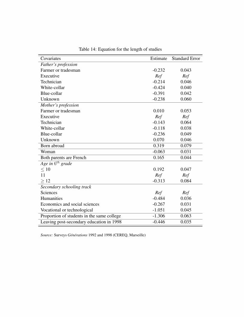
Table 14: Equation for the length of studies

Covariates Estimate Standard ErrorFather’s professionFarmer or tradesman -0.232 0.043Executive Ref RefTechnician -0.214 0.046White-collar -0.424 0.040Blue-collar -0.391 0.042Unknown -0.238 0.060Mother’s professionFarmer or tradesman 0.010 0.053Executive Ref RefTechnician -0.143 0.064White-collar -0.118 0.038Blue-collar -0.236 0.049Unknown 0.070 0.046Born abroad 0.319 0.079Woman -0.063 0.031Both parents are French 0.165 0.044Age in 6th grade≤ 10 0.192 0.04711 Ref Ref≥ 12 -0.313 0.084Secondary schooling trackSciences Ref RefHumanities -0.484 0.036Economics and social sciences -0.267 0.031Vocational or technological -1.051 0.045Proportion of students in the same college -1.306 0.063Leaving post-secondary education in 1998 -0.446 0.035


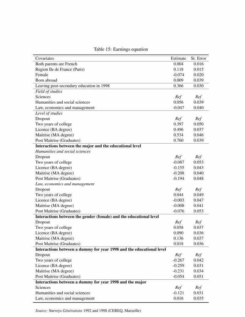
Table 15: Earnings equation

Covariates Estimate St. ErrorBoth parents are French 0.004 0.016Region Ile de France (Paris) 0.118 0.015Female -0.074 0.020Born abroad 0.009 0.039Leaving post-secondary education in 1998 0.366 0.030Field of studiesSciences Ref RefHumanities and social sciences 0.056 0.039Law, economics and management -0.047 0.040Level of studiesDropout Ref RefTwo years of college 0.397 0.050Licence (BA degree) 0.496 0.037Maitrise (MA degree) 0.534 0.046Post Maitrise (Graduates) 0.760 0.039Interactions between the major and the educational levelHumanities and social sciencesDropout Ref RefTwo years of college -0.087 0.053Licence (BA degree) -0.155 0.043Maitrise (MA degree) -0.208 0.040Post Maitrise (Graduates) -0.194 0.048Law, economics and managementDropout Ref RefTwo years of college 0.044 0.049Licence (BA degree) -0.003 0.047Maitrise (MA degree) -0.008 0.041Post Maitrise (Graduates) -0.076 0.053Interactions between the gender (female) and the educational levelDropout Ref RefTwo years of college 0.058 0.037Licence (BA degree) 0.090 0.036Maitrise (MA degree) 0.136 0.037Post Maitrise (Graduates) 0.018 0.036Interactions between a dummy for year 1998 and the educational levelDropout Ref RefTwo years of college -0.267 0.042Licence (BA degree) -0.259 0.031Maitrise (MA degree) -0.231 0.034Post Maitrise (Graduates) -0.054 0.051Interactions between a dummy for year 1998 and the majorSciences Ref RefHumanities and social sciences -0.121 0.031Law, economics and management 0.016 0.035


Table 16: Other parameters

Covariance matrix of residuals (standard errors in parentheses)

1 0 0 00 1 1.053 0

(−) (−) (0.129) (−)0 1.053 2.379 0

(−) (0.129) (0.318) (−)0 0 0 0.516

(−) (−) (−) (0.005)

Estimate St. Error

Thresholdss2 -2.556 0.067s3 -2.154 0.070s4 -1.472 0.067s5 -0.710 0.069Type probabilitiesType 1 0.380 0.004Type 2 0.337 0.004Type 3 0.283 0.004


33

Table 17: Type-specific heterogeneity parameters

Estimate St. ErrorType 1α(1.1) 0.000 -α(1.2) 1.244 0.091α(1.3) 1.037 0.093α2 0.000 -α3 8.192 0.038Type 2α(1.1) 0.000 -α(1.2) -1.312 0.091α(1.3) -2.828 0.141α2 -0.363 0.043α3 8.111 0.032Type 3α(1.1) 0.000 -α(1.2) -1.363 0.082α(1.3) -1.571 0.119α2 0.502 0.051α3 8.089 0.036


Table 18: Estimated proportions of students in each major, at each level of post-secondary edu-cation, by type

Major Type 1 Type 2 Type 3Sciences 0.00 44.66 50.34Humanities and Social Sciences 41.02 55.34 17.49Law, Business and Management 58.98 0.00 32.16Length Type 1 Type 2 Type 3Dropout 26.40 47.55 0.00Two years of college 12.43 16.73 0.86Licence (BA degree) 26.81 24.42 4.58Maitrise (MA degree) 19.77 10.53 29.43Post Maitrise (Graduates) 14.58 0.77 65.14


34

Table 19: Estimated means and standard errors of log-earnings distributions, by type

Mean St.ErrorWhole sample 8.65 0.57Type 1 8.62 0.32Type 2 8.48 0.31Type 3 8.84 0.29


35

C Simulation exercises with risk aversion and log-earningsheteroskedasticity

Table 20: Simulation of a 10% variation in expected earnings associated with majors in sciences(percentages)



Sciences 28.67 26.21 0.214 0.004Humanities and Social Sciences 37.59 40.18 -0.070 0.003Law, Economics and Management 33.75 33.61 -0.144 0.005

10% decreaseSciences 28.67 26.21 -0.234 0.004Humanities and Social Sciences 37.59 40.18 0.077 0.003Law, Economics and Management 33.75 33.61 0.157 0.006Source: Surveys Générations 1992 and 1998 (CEREQ, Marseille).


Table 21: Simulation of a 10% variation in expected earnings associated with majors in humani-ties and social sciences



Sciences 28.67 26.21 -0.066 0.003Humanities and Social Sciences 37.59 40.18 0.311 0.015Law, Economics and Management 33.75 33.61 -0.245 0.017

10% decreaseSciences 28.67 26.21 0.073 0.003Humanities and Social Sciences 37.59 40.18 -0.347 0.017Law, Economics and Management 33.75 33.61 0.274 0.019Source: Surveys Générations 1992 and 1998 (CEREQ, Marseille).


36

Table 22: Simulation of a 10% variation in expected earnings associated with majors in law,economics and management (percentages)



Sciences 28.67 26.21 -0.146 0.005Humanities and Social Sciences 37.59 40.18 -0.242 0.017Law, Economics and Management 33.75 33.61 0.388 0.021

10% decreaseSciences 28.67 26.21 0.163 0.006Humanities and Social Sciences 37.59 40.18 0.269 0.018Law, Economics and Management 33.75 33.61 -0.432 0.023Source: Surveys Générations 1992 and 1998 (CEREQ, Marseille).


37

Documents

Choosing the Field of Study in Post-Secondary Education ...ftp.iza.org/dp4127.pdf · Choosing the Field of Study in Post-Secondary Education: Do Expected Earnings Matter? Magali Beffy