Chlorophyll-a patterns and mixing processes in the … · Las imágenes diarias del sensor MODIS a bordo del satélite Aqua permitieron identificar los patrones superficiales de la

Ciencias Marinas (2014), 40(1): 11–31

11

CM

http://dx.doi.org/10.7773/cm.v40i1.2320

Chlorophyll-a patterns and mixing processes in the Yucatan Basin,Caribbean Sea

Patrones superficiales de la clorofila a y procesos de mezcla en lacuenca de Yucatán, mar Caribe

Iván Pérez-Santos1,2*, Wolfgang Schneider1, Arnoldo Valle-Levinson3, José Garcés-Vargas4,Inia Soto5,6, Raúl Montoya-Sánchez2, Nelson Melo González7, Frank Müller-Karger5

1 Departamento de Oceanografía, Universidad de Concepción, Campus Concepción, Víctor Lamas 1290, Casilla 160-C, CP 4070043, Concepción, Chile.

2 Centro de Investigación Oceanográfica en el Pacifico Sur-Oriental (COPAS Sur Austral), Universidad de Concepción, Campus Concepción, Víctor Lamas 1290, Casilla 160-C, CP 4070043, Concepción, Chile.

3 Department of Civil and Coastal Engineering, University of Florida, Gainesville, FL 32611, USA.4 Instituto de Ciencias Marinas y Limnológicas, Facultad de Ciencias, Universidad Austral de Chile,

Edificio Pugín, Campus Isla Teja, Chile.5 Institute for Marine Remote Sensing, College of Marine Science, University of South Florida, St. Petersburg,

FL 33701, USA.6 Laboratório de Estudos dos Oceano e Clima, Universidade Federal do Rio Grande, Rio Grande,

Rio Grande do Sul, CEP 96.201-900, Brasil.7 Physical Oceanography Division, NOAA/Atlantic Oceanographic and Meteorological Laboratory -

Rosenstiel School of Marine and Atmospheric Science/Cooperative Institute for Marine and Atmospheric Studies of the University of Miami, 4301 Rickenbacker Causeway Miami, FL 33149-1026, USA.

* Corresponding author. E-mail: [email protected]

ABSTRACT. Daily images collected with the MODIS sensor on the NASA Aqua satellite were used to describe chlorophyll-a (chl-a)concentrations before, during, and after synoptic-scale meteorological pulses in the Yucatan Basin, Caribbean Sea. The relative influence ofvertical diffusive and vertical advective transport on mixing of the near surface layer was quantified with wind data from the QuikSCATsatellite. Computation of vertical density eddy diffusivity and gradient Richardson numbers was done with data from the three-dimensionalMERCATOR model. The model evidenced the importance of vertical shear (i.e., vertical diffusive processes) in generating mixing duringautumn and winter (2007–2009). During moderate meteorological pulses (e.g., cold fronts, easterly tropical waves, and low-pressure systemswith wind speeds of 9–15 m s–1 sustained over 2 days), mixing caused by diffusive transport (eddy viscosity of 10 10–3 m2 s–1) was at leastone order of magnitude higher than upward advective mixing (0.3 10–3 m2 s–1). During the passage of hurricanes Ivan (September 2004) andWilma (October 2005), upward advective mixing (5–7 m2 s–1) dominated mixing of the upper water column and was nearly four orders ofmagnitude higher than during moderate meteorological events. Background chl-a concentrations of 0.03–0.08 mg m–3 were observed duringthe July–October period. During synoptic weather pulses, three different patterns in the chl-a concentrations were observed: first, chl-aconcentrations in the range of 0.05 to 0.12 mg m–3 followed moderate meteorological pulses; second, higher regional chl-a concentrations(0.5–2.0 mg m–3) followed the passage of hurricanes; and third, the formation of filaments showing apparent high chl-a (0.3–1.5 mg m–3) southof Cuba, possibly caused by freshwater discharge from land. The changes in chlorophyll patterns following meteorological events illustratetypical patterns of connectivity among different parts of the Yucatan Basin.

Key words: satellite chlorophyll-a, wind mixing, vertical transport, surface currents, Yucatan Basin.

RESUMEN. Las imágenes diarias del sensor MODIS a bordo del satélite Aqua permitieron identificar los patrones superficiales de laclorofila a antes, durante y después del paso de eventos meteorológicos de escala sinóptica por la cuenca de Yucatán, mar Caribe. Los datos deviento superficial del satélite QuikSCAT se utilizaron para cuantificar la influencia del transporte vertical advectivo y la difusividad vertical enla mezcla de la capa superficial del mar. Los datos del modelo tridimensional MERCATOR permitieron el cálculo de la difusividad vertical deremolino y el número de Richardson, evidenciando la importancia de la cizalladura vertical durante las épocas de otoño e invierno(2007–2009). Durante el paso de eventos sinópticos moderados (e.g., frentes fríos, ondas tropicales del este y sistemas de baja presión convientos de 9 a 15 m s–1 sostenidos durante dos días), la mezcla causada por la difusividad vertical (10 × 10–3 m2 s–1) fue al menos un orden demagnitud mayor que el transporte vertical advectivo (0.3 × 10–3 m2 s–1). Sin embargo, durante el paso de los huracanes Iván (septiembre de2004) y Wilma (octubre de 2005), el transporte vertical advectivo (5–7 m2 s–1) dominó la mezcla de la columna de agua y fue cuatro órdenes demagnitud mayor al registrado durante la influencia de los eventos moderados. Bajo la influencia de estos eventos meteorológicos, seobservaron tres patrones en la clorofila a: en el primero se encontraron concentraciones de clorofila a en el rango de 0.05 a 0.12 mg m–3

Ciencias Marinas, Vol. 40, No. 1, 2014

12

INTRODUCTION

Satellite-derived chlorophyll-a (chl-a) concentrations,computed based on the ratio of seawater-leaving radiancesobtained by ocean color sensors, have been applied to studythe temporal and spatial variability of highly productiveupwelling systems (e.g., Peláez and McGowan 1986,McClain 2009), as well as the functioning of oligotrophicsystems (e.g., Babin et al. 2004). Maximum chl-a concentra-tions in upwelling systems are reached when the availabilityof nutrients and solar radiation to phytoplankton are optimal,and grazing is minimal. In oligotrophic regions, high chl-alevels can occur when well-lit surface waters experience abreak-down in thermal stratification and increased mixingdue to wind, resulting in the availability of nutrients from thesubsurface layer (Müller-Karger et al. 1991, González et al.2000).

By analyzing satellite-derived chl-a from the CoastalZone Color Scanner (CZCS), Müller-Karger et al. (1991)obtained the first multi-year time series of monthly meansurface chl-a concentrations for the oligotrophic Gulf ofMexico and the northwestern Caribbean Sea; they observedhigher Chl-a concentrations from December to February(>0.18 mg m–3) and lower concentrations in May and June(0.06 mg m–3). The deepening/shoaling of the mixed layerwas found to be a major factor controlling chl-a seasonality.González et al. (2000) further examined these patterns ofphytoplankton concentrations in the Caribbean Sea, the Gulfof Mexico, and the Sargasso Sea, and discovered that thehighest chl-a concentrations were associated with highervertical mixing after the passage of cold fronts.

Off southwestern Cuba and in the Yucatan Basin, coldfronts from the northwest are frequent from October to April.On average, about 11 to 35 cold fronts affect the area everyyear, with a historic mean of 19.8 ± 4.9 for the winter season(González 1999). In addition, easterly tropical waves occur inthe tropical North Atlantic from June to November and cangenerate hurricanes in the region.

Different studies have characterized chl-a distributions atthe seasonal scale in the western Caribbean Sea. In particular,the Yucatan Basin is affected by weather phenomena year-round, including moderate (e.g., cold fronts, easterly tropicalwaves, low pressure systems) and extreme (hurricanes)meteorological forcing (Pérez-Santos et al. 2010). In thismanuscript we describe chl-a distributions in the YucatanBasin at synoptic scales and assess their response to windsand circulation regime.

INTRODUCCIÓN

Las concentraciones de clorofila a, estimadas con base enla razón de las radiancias emergentes del agua obtenidas pormedio de sensores remotos que miden el color del océano,han sido usadas para estudiar la variabilidad temporal yespacial de sistemas de surgencia altamente productivos(e.g., Peláez y McGowan 1986, McClain 2009), así como elfuncionamiento de sistemas oligotróficos (e.g., Babin et al.2004). Las máximas concentraciones de clorofila a en lossistemas de surgencia suceden cuando la disponibilidad denutrientes y la radiación solar sobre el fitoplancton sonóptimas y el pastoreo es mínimo. En regiones oligotróficas,se obtienen altos niveles de clorofila a cuando se rompe laestratificación termal de las aguas superficiales bien ilumina-das e incrementa la mezcla debido al viento, con la conse-cuente disponibilidad de nutrientes de la capa subsuperficial(Müller-Karger et al. 1991, González et al. 2000).

Mediante el análisis de datos obtenidos con el sensorCoastal Zone Color Scanner (CZCS), Müller-Karger et al.(1991) obtuvieron, por primera vez, una serie de tiempo mul-tianual de la concentración media superficial de clorofila apara las aguas oligotróficas del golfo de México y el marCaribe noroccidental, observándose mayores concentracionesde clorofila a entre diciembre y febrero (>0.18 mg m–3) ymenores concentraciones en mayo y junio (0.06 mg m–3). Elhundimiento de la capa de mezcla jugó un papel importanteen la estacionalidad de la clorofia a. González et al. (2000)examinaron los patrones de las concentraciones de fitoplanc-ton en el mar Caribe, el golfo de México y el mar de losSargazos, y descubrieron que las mayores concentracionesde clorofila a se asociaban con una mayor mezcla verticaldespués del paso de frentes fríos.

Al suroeste de Cuba y en la cuenca de Yucatán, los frentesfríos del noroeste son frecuentes de octubre a abril. En pro-medio, de 11 a 35 frentes fríos afectan el área cada año, conuna media histórica de 19.8 ± 4.9 para el invierno (González1999). Además, se presentan ondas tropicales del este en elAtlántico Norte tropical entre junio y noviembre, los cualespueden generar huracanes en la región.

Distintos estudios han caracterizado la distribución declorofila a a escala estacional en el mar Caribe occidental. Enparticular, la cuenca de Yucatán se ve afectada por fenó-menos climáticos todo el año, incluyendo forzamientosmeteorológicos moderados (e.g., frentes fríos, ondas tropica-les del este, sistemas de baja presión) y extremos (huracanes)(Pérez-Santos et al. 2010). En el presente trabajo se describe

después del paso de eventos meteorológicos moderados, en el segundo se hallaron máximos de clorofila a (0.5–2.0 mg m–3) después del paso delos huracanes Iván y Wilma, y en el tercero se observó la presencia de concentraciones altas de clorofila a (0.3–1.5 mg m–3) en forma defilamentos debido a las descargas de aguas dulces desde la isla de Cuba. Los cambios en los patrones superficiales de clorofila después del pasode eventos meteorológicos evidenciaron los patrones típicos de conectividad entre las diferentes áreas de la cuenca de Yucatán.

Palabras clave: clorofila a satelital, mezcla por viento, advección vertical, corrientes superficiales, cuenca de Yucatán.

Pérez-Santos et al.: Chlorophyll-a and mixing in the Yucatan Basin

13

MATERIALS AND METHODS

Study area

The study area covers the region between 18º and 23º N,and between 80º and 89º W (fig. 1). The region encompassesthe Yucatan and Cayman basins, the continental shelf northof the Yucatan Peninsula, and the northern portion of theMesoamerican Reef System (off the southeastern coast ofMexico and northern Belize).

The Yucatan Basin is located in the area known as theAtlantic warm pool (Wang and Lee 2007), which strengthensduring the boreal summer and early autumn. Sea surface tem-peratures may exceed 28.5 ºC, leading to a significant impacton tropical atmospheric convection (Wang and Enfield 2001).The surface wind stress shows a maximum during Novemberas the Atlantic warm pool weakens, and a secondary maxi-mum in June related to the intensification of the Caribbeanlow-level jet (Pérez-Santos et al. 2010).

Surface wind data from satellites

Surface wind data obtained from the SeaWinds scatter-ometer onboard the NASA QuikSCAT satellite were used tocalculate wind stress and wind curl. Daily gridded oceanwind vectors with a spatial resolution of 0.5º 0.5º weredownloaded from IFREMER (Institut Français de Recherchepour l’Exploitation de la Mer). The analysis of satellitewind data covered the period from 21 November 1999 to21 November 2009.

The Hurricane Research Division (HRD) of the NOAAAtlantic Oceanographic and Meteorological Laboratory(AOML) maintains a high-resolution surface wind speeddatabase (H-Wind product) for particular storm events (http://www.aoml.noaa.gov/hrd). We used this database specificallyto examine the passage of hurricanes Ivan (13 September2004, 0130 UTC) and Wilma (20 October 2005, 1330 UTC)through the Yucatan Basin and because QuikSCAT scatter-ometers underestimate the magnitude of wind during extremeevents (Donelan et al. 2004). The H-Wind product integratesall of the available observations every 6 h with a spatial reso-lution of 6 6 km.

MERCATOR assimilation model data

Results of the three-dimensional MERCATOR assimila-tion model PSY2V3R1 ATL12 were used to understandthe ocean mixing processes (model available at http://www.mercator-ocean.fr). Since 2007, the daily output ofthe MERCATOR model is distributed at a spatial resolutionof 1/12º (9 9 km) and 43 vertical levels. Model outputconsisting of three-dimensional ocean currents, watertemperature, and salinity was extracted from 2007 to 2009 at36 vertical levels for a domain covering the northwesternCaribbean Sea between 18º–21.5º N and 80º–88º W. The

la distribución de clorofila a en la cuenca de Yucatán a escalasinóptica y se evalúa su respuesta al régimen de circulación yvientos.

MATERIALES Y MÉTODOS

Área de estudio

El área de estudio comprende la región entre 18º y 23º Ny entre 80º y 89º W (fig. 1). La región incluye las cuencas deYucatán y Caimán, la plataforma continental al norte de lapenínsula de Yucatán y la parte norte del Sistema ArrecifalMesoamericano (costa sudoriental de México y Belice).

La cuenca de Yucatán se localiza en la zona conocidacomo la alberca caliente del Atlántico (Wang y Lee 2007),que se fortalece durante el verano boreal y a principios deotoño. La temperatura superficial del mar puede excederlos 28.5 ºC y tener un fuerte impacto en la convecciónatmósferica tropical (Wang y Enfield 2001). El esfuerzo delviento superficial muestra un máximo en noviembre cuandose debilita la alberca caliente del Atlántico y un segundomáximo en julio relacionado con la intensificación del chorrode bajo nivel del Caribe (Pérez-Santos et al. 2010).

Datos satelitales de viento superficial

Para calcular el esfuerzo del viento y su rotacional, seusaron datos de viento superficial proporcionados por eldispersómetro SeaWinds a bordo del satélite QuikSCAT(NASA). Se obtuvieron vectores diarios del viento en lasuperficie del mar con una resolución espacial de 0.5º 0.5ºde IFREMER (Institut Français de Recherche pour l’Exploi-tation de la Mer). El análisis de los datos de viento satelitalescubrió el periodo del 21 de noviembre de 1999 al 21 denoviembre de 2009.

La División de Investigación de Huracanes del Laborato-rio Oceanográfico y Meteorológico del Atlántico (HRD-AOML/NOAA, por sus siglas en inglés) mantiene una basede datos de alta resolución de la velocidad de vientosuperficial (H-Wind Project) para ciertas tormentas (http://www.aoml.noaa.gov/hrd). Se usó esta base de datos especí-ficamente para analizar el paso de los huracanes Iván (13 deseptiembre de 2004, 0130 UTC) y Wilma (20 de octubre de2005, 1330 UTC) por la cuenca de Yucatán y porque losdispersómetros de QuikSCAT subestiman la magnitud delviento durante eventos extremos (Donelan et al. 2004). Estabase de datos integra todas las observaciones disponiblescada 6 h con una resolución espacial de 6 6 km.

Datos del modelo de asimilación MERCATOR

Para entender los procesos de mezcla en el oceáno, seusaron los datos del modelo tridimensional de asimilaciónMERCATOR PSY2V3R1 ATL12, disponible en http://www.mercator-ocean.fr. Desde 2007, los resultados diarios


14

circulation patterns obtained with the MERCATOR model(supplement 1) agree with general circulation patterns gener-ated by different ocean models for this region (e.g., Johnset al. 2002, Centurioni and Niiler 2003, Romanou et al. 2004,Jouanno et al. 2008).

Quantification of mixing processes

In order to quantify the influence of vertical advectivetransport and vertical diffusive transport on the mixing of thesea surface layer, the vertical advective transport (Wad) andthe vertical eddy viscosity (Az) were calculated. To estimateWad (Wad = WEDE), the product of the Ekman pumpingvelocity (WE) and Ekman layer depth (DE) was determined.Positive values of Wad denoted upwelling and negative values

indicated downwelling; negative values were excluded fromthe resulting figure in order to represent only the results ofWad related to the upwelling process.

WE was calculated from the wind stress curl according toSmith (1968):

del modelo MERCATOR se distribuyen con una resoluciónespacial de 1/12º (9 9 km) y 43 niveles verticales. La pro-ducción del modelo, consistente en datos de temperatura ysalinidad del agua y corrientes oceánicas tridimensionales, seobtuvo de 2007 a 2009 en 36 niveles verticales para un domi-nio cubriendo el mar Caribe noroccidental entre 18º–21.5º Ny 80º–88º W. Los patrones de circulación obtenidos con elmodelo MERCATOR (suplemento 1) coinciden con lospatrones generales generados por diferentes modelos paraesta región (e.g., Johns et al. 2002, Centurioni y Niiler 2003,Romanou et al. 2004, Jouanno et al. 2008).

Cuantificación de los procesos de mezcla

Para cuantificar la influencia del transporte verticaladvectivo y la difusividad vertical en la mezcla de la capasuperficial del mar, se calcularon el transporte vertical advec-tivo (Wad) y la viscosidad vertical de remolino (Az). Paraestimar Wad (Wad = WEDE), se determinó el producto de lavelocidad de bombeo de Ekman (WE) y la profundidad de lacapa de Ekman (DE). Los valores positivos de Wad indican

Figure 1. Bathymetric map (ETOPO-8.2) of the study area. Black dots represent the QuikSCAT wind product grid. Open circles show thelocations where the strength of vertical transport and vertical eddy viscosity were computed. Red dots indicate the positions of theMERCATOR time series used to calculate vertical eddy diffusivity, gradient Richardson number, buoyancy frequency squared, and verticalshear flow. Bathymetry is shown in grey shading according to the scale on the right-hand side of the figure.Figura 1. Mapa batimétrica (ETOPO-8.2) del área de estudio. Los puntos negros representan la red de datos de viento de QuikSCAT. Loscírculos abiertos muestran los sitios donde se estimaron el transporte vertical advectivo y la viscosidad vertical de remolino. Los puntos rojosindican las posiciones de la serie de tiempo de MERCATOR que se usaron para calcular la difusividad vertical de remolino, el número deRichardson, la frecuencia de flotabilidad al cuadrado y la cizalladura vertical. La batimetría se muestra en tonos de gris según la escala a laderecha de la figura.

Gulf of Mexico

Mexico

Longitude (°W)

Latit

ude

(°N

)

Northern Yucatan Shelf

23

22.5

22

21.5

21

20.5

20

19.5

19

18.5

18

YucatanPeninsula

Pinar del RioCuba

Depth (m)

89 88 87 86 85 84 83 82 81 80

-2000

-1000

-4000

-3000

-6000

-5000


15

(1)

where is the wind stress curl and ρ is water density;f = 2sin() is the Coriolis parameter ( is latitude). Thewind stress curl was obtained through first-order finite cen-tered differences. Cokriging extrapolation (Marcotte 1991)was applied to increase the resolution of wind stress curl datanear the coast.

Wind stress (τ) was calculated by quadratic parameteriza-tion (τx = ρairCdU10x|U10s| and τy = ρairCdU10y|U10s| for the zonal(east-west) and for the meridional (north-south) components,respectively, where U10x and U10y are the wind components at10 m height and U10s is the wind magnitude at 10 m height).The drag coefficient (Cd) was calculated as in Yelland andTaylor (1996) except during hurricanes Ivan and Wilma, forwhich wind stress was calculated using a constant drag coef-ficient of 2.8 × 10–3 (Donelan et al. 2004).

DE (meters), at latitudes () beyond +/–10º of the equator,was computed as follows (Pond and Pickard 1983):

(2)

Then, Az was estimated according to Stewart (2008):

(3)

Values for Wad, Az, and DE were obtained for each gridpoint of the QuikSCAT and H-Wind products. A time seriesof average values for each product was generated for theentire study domain. The time series at two specific points(fig. 1, open circles) were also chosen to illustrate changesnear Cuba (21.7º N, 83.7º W) and off the Yucatan Peninsulain the Caribbean Sea, south of the island of Cozumel(19.7º N, 87.2º W). We sought to examine the relative contri-butions of Wad and Az diffusive transport in the Ekman layerdepth as sources of nutrients from the subsurface to the sur-face. Wad represented the influence of the wind stress curl andpumping, and Az indicated the frictional effects caused by thesurface wind.

Eddy viscocity represents the diffusivity of momentumassociated with the wind stress. To also account for diffusiv-ity of mass, the vertical eddy diffusivity (Kv) was obtainedfrom the temperature, salinity, and velocity profiles from thethree-dimensional output of the MERCATOR model.

Kv was computed using the parameterization proposed byRodríguez-Santana et al. (1999), which incorporates tworegimes: (a) low gradient Richardson number (Ri) values,Kv = 1.1 × 10–8 Ri–9.2, Ri 0.33, and (b) high Ri values,

WE f

-------------=

DE4.3

sin -----------------------U10s=

Az

DE2 f

22---------=

surgencia y los valores negativos, hundimiento; en la figuraresultante los valores negativos fueron excluidos y sólo semuestran los resultados de Wad favorables a la surgencia.

Se calculó WE a partir del rotacional del esfuerzo delviento según Smith (1968):

(1)

donde es el rotacional del esfuerzo del viento y ρ es ladensidad del agua; f = 2sin() es el parámetro de Coriolis( es la latitud). El rotacional del esfuerzo del viento seobtuvo a partir de diferencias finitas centradas de primerorden. Se realizó una extrapolación tipo “cokriging”(Marcotte 1991) para incrementar la resolución de los datosdel rotacional del esfuerzo del viento cerca de la costa.

El esfuerzo del viento (τ) se calculó mediante laparametrización cuadrática (τx = ρaireCdU10x|U10s| y τy =ρaireCdU10y|U10s| para los componentes zonal (este-oeste) ymeridional (norte-sur), respectivamente, donde U10x y U10y

son las componentes del viento a 10 m de altura y U10s es lamagnitud del viento a 10 m de altura). El coeficiente de arras-tre (Cd) se calculó siguiendo a Yelland y Taylor (1996),excepto durante los huracanes Iván y Wilma, cuando elesfuerzo del viento se calculó con un coeficiente de arrastreconstante de 2.8 × 10–3 (Donelan et al. 2004).

Se calculó DE (metros), a latitudes () +/–10º del ecuador,como sigue (Pond y Pickard 1983):

(2)

Luego, se estimó Az según Stewart (2008):

(3)

Los valores para Wad, Az y DE fueron obtenidos para cadapunto de las redes de los productos de H-Wind y QuikSCAT.Se generó una serie de tiempo de valores promedios paracada producto para toda la zona de estudio. También seeligieron las series de tiempo de dos puntos específicos(fig. 1, círculos abiertos) para ilustrar los cambios cerca deCuba (21.7º N, 83.7º W) y de la península de Yucatán en elmar Caribe, al sur de la isla de Cozumel (19.7º N, 87.2º W).Se pretendió analizar las contribuciones relativas de Wad y eltransporte difusivo de Az en la profundidad de la capa deEkman como fuentes de nutrientes de la subsuperficie a lasuperficie; Wad representó la influencia del rotacional delesfuerzo del viento y el bombeo, y Az indicó los efectos defricción causados por el viento en la superficie.

WE f

-------------=

DE4.3

sin -----------------------U10s=

Az

DE2f

22---------=


16

Kv = 2.6 × 10–3 (1 + 10Ri)–3/2, Ri 0.33. Ri was defined asfollows:

(4)

where N is the buoyancy frequency, representing the stabilityof the water column, and S2 is the vertical shear flow. S2 wascalculated using vertical central differences:

(5)

where u and v are the zonal and meridional current compo-nents obtained from the MERCATOR model. Values of Kv,Ri, N2, and S2 were computed at three different locations(fig. 1, red points): Yucatan Basin (20.1º N, 84º W), south-west of Cuba (21.5º N, 83.8º W), and southeast of theYucatan Peninsula (19.6º N, 87.2º W).

Satellite chlorophyll-a data

Satellite-derived images of chl-a concentrations wereobtained from the Moderate Resolution Imaging Spectroradi-ometer (MODIS) sensor onboard the Aqua satellite. MODIS-Aqua provides a daily product of surface ocean chl-aconcentration with a spatial resolution of approximately1 km2 per pixel at nadir over cloud-free ocean areas. Chl-aconcentrations for the Yucatan Basin (18º–22º N,80º–86.5º W) were extracted using SeaDAS 6.1 software.

To confirm that the chl-a patterns observed were indeedrelated to phytoplankton blooms, the fluorescence line height(FLH) products from MODIS-Aqua were also analyzed.These FLH products were processed similarly to chl-aproducts following Letelier and Abbott (1996). For purposesof this study, shallow areas or those near the coast were notconsidered for the chl-a or FLH analysis (e.g., Gulf ofBatabanó, fig. 1).

To investigate the ocean response to synoptic-scalemeteorological events, daily chl-a concentration and FLHimages were analyzed before, during, and after hurricanesIvan (2–24 September 2004) and Wilma (15–25 October2005). Other synoptic-scale meteorological events were alsoanalyzed in 2004 and 2005, such as cold fronts, low-pressuresystems, and tropical waves. For this paper we selected oneor two relatively cloud-free images that best represented thechl-a distributions associated with each wind event.

Dynamic topography obtained from altimetry

We used the Salto/Duacs altimeter products developedby the CNES (Centre National d’Études Spatiales, France;http://www.aviso.oceanobs.com/). This database has a tem-poral resolution of 7 days and a spatial resolution of 1/3º. The

RiN2

S2------=

S2 u

z------

2 vz-----

2

+=

La viscosidad de remolino representa la difusividad demomento asociada con el esfuerzo del viento. Para tambiénconsiderar la difusividad de masa, se obtuvo la difusividadvertical de remolino (Kv) de los perfiles de temperatura, sali-nidad y velocidad de los resultados tridimensionales delmodelo MERCATOR.

Se calculó Kv mediante la parametrización propuestapor Rodríguez-Santana et al. (1999), la cual incorpora dosregímenes: (a) valores bajos del número de Richardson (Ri),Kv = 1.1 × 10–8 Ri–9.2, Ri 0.33, y (b) valores altos de Ri,Kv = 2.6 × 10–3 (1 + 10Ri)–3/2, Ri 0.33. Se definió Ri comosigue:

(4)

donde N es la frecuencia de flotabilidad, representando laestabilidad de la columna de agua, y S2 es la cizalladura verti-cal. Esta última se calculó usando diferencias centrales en lavertical:

(5)

donde u y v son los componentes zonal y meridional de lacorriente obtenidos del modelo MERCATOR. Los valores deKv, Ri, N2 y S2 fueron calculados en tres sitios distintos(fig. 1, puntos rojos): la cuenca de Yucatán (20.1º N, 84º W),al suroeste de Cuba (21.5º N, 83.8º W) y al sureste de lapenínsula de Yucatán (19.6º N, 87.2º W).

Datos satelitales de clorofila a

Las imágenes de clorofila superficial fueron provistas porel sensor Moderate Resolution Imaging Spectroradiometer(MODIS) a bordo del satélite Aqua. Este sensor proporcionadatos diarios de la concentración de clorofila a en la superfi-cie del mar con una resolución espacial de aproximadamente1 km2 por pixel al nadir sobre áreas del océano libres denubes. Las concentraciones de clorofila a para la cuenca deYucatán (18º–22º N, 80º–86.5º W) fueron obtenidas con elpaquete SeaDAS 6.1.

Para confirmar que los patrones de clorofila a estuvieranefectivamente relacionados con afloramientos fitoplanctó-nicos, también se analizaron los datos de la altura de la líneade fluorescencia (FLH, por sus siglas en inglés) de MODIS-Aqua. Estos datos fueron procesados de forma similar a losde clorofila a siguiendo a Letelier y Abbott (1996). Para elpropósito de este estudio, no se consideraron zonas someras ocerca de la costa para el análisis de FLH o clorofila a(e.g., golfo de Batabanó, fig. 1).

Para analizar la respuesta del océano a fenómenos meteo-rológicos de escala sinóptica, se analizaron imágenes diarias

RiN

2

S2------=

S2 uz------

2 vz-----

2

+=


17

zonal and meridional components of the absolute geostrophiccurrents were obtained from the MADT (Map of AbsoluteDynamic Topography) product distributed by CNES.

RESULTS

Quantification of mixing processes

The three time series of vertical eddy viscosity (Az)showed a similar annual cycle that peaked in November andDecember (10–15 × 10–3 m2 s–1; fig. 2a–c). Starting in Janu-ary, Az diminished reaching its lowest value (~3 × 10–3 m2 s–1)around the beginning of September. A small secondary rela-tive maximum was observed in June (10–12 × 10–3 m2 s–1). Ingeneral, vertical transport velocities (Wad) were two orders ofmagnitude lower than the values of Az and they were alwaysfavorable to upwelling (positive values). No annual cycle forWad could be observed in the averages for the entire region(fig. 2d–f). Several isolated maxima, at least one order ofmagnitude higher than the regional average, could beobserved in the climatology off southern Cuba in May/Juneand October/November, corresponding to the hurricaneseason in the region. The Ekman layer depth (DE) rangedfrom 40 to 60 m all year round, with the minimum(maximum) during the summer (winter). Minimum DE was

also registered in September (fig. 2g–i).The maximum values of vertical eddy diffusivity (Kv)

were found near the mixed layer depth in the region, as char-acterized by the three different locations, with magnitudes ofKv = 10–5–10–3 m2 s–1 (fig. 3a–c). The time series of Kv foreastern Yucatan was different from the series for southernCuba and the central Yucatan Basin, showing high variabilitybelow the mixed layer depth, from 50 to 250 m depth. Itsseasonal median was one order of magnitude higher, with thegreatest Kv (0.27 m2 s–1) at midyear (table 1). As expected, thegradient Richardson number (Ri) was inversely related to Kv

(fig. 3d–f). Low values of Ri were observed during springand summer, indicating favorable conditions for verticalmixing, but strong stratification led instead to high buoyancyfrequency (N2, 2–4 10–4 s–2) and decreased mixing(fig. 3g–i). Vertical shear (S2) was high in the first 50 m(10–5–10–4 s–2) of the water column, with a second maximumzone between 70 and 200 m (fig. 3j–l). Maximum values ofS2 reached the surface in spring and summer, and deepened inautumn and winter.

Analysis of vertical advective transport (Wad), vertical eddy viscosity (Az), and Ekman layer depth (DE) during synoptic-scale meteorological events

Cold front

During the influence of a cold front (7 November 2004),winds were northerly with mean velocities of 8.7 m s–1 andwind stress increased toward the south with maximum values

de la concentración de clorofila a y FLH antes, durante y des-pués de los huracanes Iván (2–24 de septiembre de 2004) yWilma (15–25 de octubre de 2005). También se analizaronotros eventos meteorológicos de escala sinóptica en 2004 y2005, tales como frentes fríos, sistemas de baja presión yondas tropicales. Para este estudio, se seleccionaron una odos imágenes relativamente libres de nubes que mejor repre-sentaban la distribución de clorofila a asociada con cadaevento.

Topografía dinámica obtenida por altimetría

Se usaron los datos del altímetro Salto/Duacs proporcio-nados por CNES (Centre National d’Études Spatiales,Francia; http://www.aviso.oceanobs.com/). Esta base dedatos tiene una resolución temporal de 7 días y una resolu-ción espacial de 1/3º. Los componentes zonal y meridional delas corrientes geostróficas absolutas fueron obtenidas delproducto MADT (Map of Absolute Dynamic Topography)distribuido por CNES.

RESULTADOS

Quantificación de los procesos de mezcla

Las tres series de tiempo de la viscosidad vertical deremolino (Az) mostraron un ciclo anual similar con valoresmáximos (10–15 × 10–3 m2 s–1) en noviembre y diciembre(fig. 2a–c). A partir de enero, la Az decreció hasta alcanzar suvalor mínimo (~3 × 10–3 m2 s–1) a principios de septiembre,observándose un segundo máximo relativo secundario enjunio (10–12 × 10–3 m2 s–1). En general, las velocidades detransporte vertical (Wad) fueron dos órdenes de magnitudmenores que los valores de Az y siempre fueron favorablespara la surgencia (valores positivos). No fue posible observarun ciclo anual para Wad en los promedios para toda la región(fig. 2d–f). Se observaron varios máximos aislados, por lomenos un orden de magnitud mayor que el promedioregional, en la climatología al sur de Cuba en mayo/junio yoctubre/noviembre, coincidiendo con la temporada de hura-canes en la región. La profundidad de la capa de Ekman (DE)osciló entre 40 y 60 m todo el año, con el mínimo (máximo)durante el verano (invierno). La DE mínima también se regis-

tró en septiembre (fig. 2g–i).Los valores máximos de la difusividad vertical de

remolino (Kv) fueron registrados cerca de la profundidad dela capa de mezcla en la región conformada por los tressitios diferentes, con magnitudes de Kv = 10–5–10–3 m2 s–1

(fig. 3a–c). La serie de tiempo de Kv para el este de Yucatándifirió de la serie para el sur de Cuba y la parte central dela cuenca de Yucatán, mostrando gran variabilidad pordebajo de la profundidad de la capa de mezcla, de 50 a250 m de profundidad. Su mediana estacional fue un ordende magnitud mayor, registrándose el valor más elevado de


18

of 0.28 Pa in the southern Yucatan Basin (fig. 4a), whichresulted in a relatively high Az (23.1 × 10–3 m2 s–1, fig. 4b).Zonal and meridional gradients of the wind stress added up toa positive wind stress curl that resulted in positive Wad values(1.3 × 10–3 m2 s–1) for most of the Yucatan Basin (fig. 4a),corresponding to extreme peaks as observed in the yearlymean time series (fig. 2).

Easterly tropical wave

From 3 to 5 July 2005, during the passage of an easterlytropical wave through the Yucatan Basin, strong winds

Kv (0.27 m2 s–1) a mediados de año (tabla 1). Como seesperaba, el número de Richardson (Ri) mostró una relacióninversa a Kv (fig. 3d–f). En primavera y verano se observaronvalores bajos de Ri, lo cual indica condiciones favorablespara la mezcla vertical; sin embargo, una fuerte estratifica-ción resultó en una frecuencia de flotabilidad alta (N2,2–4 10–4 s–2) y mezcla reducida (fig. 3g–i). La cizalladuravertical (S2) fue alta en los primeros 50 m (10–5–10–4 s–2) de lacolumna de agua, con una segunda zona máxima entre 70 y200 m (fig. 3j–l). Los valores máximos de S2 se registraronen la superficie en primavera y verano, y a mayores profundi-dades en otoño e invierno.

Average region Southern Cuba Eastern Yucatan

J F M A M J J A S O N D J F M A M J J A S O N D J F M A M J J A S O N D

Time (months)

a b c

d e f

g h i

25

20

15

10

5

0

3.0

2.5

2.0

1.5

1.0

0.5

0

90

80

70

60

50

40

30

Figure 2. An approximation of the climatology (yearly means for the period 21 November 1999 to 21 November 2009). Red lines show theseasonal variation of (a–c) vertical eddy viscosity coefficient (Az), (d–f) vertical transport (Wad), and (g–i) surface Ekman layer depth (DE).Black lines correspond to a 30-day Lanczos cosine low-pass filtered time series. Grey lines represent the positive standard deviations. The leftcolumn depicts the regional average including all QuikSCAT grid points. The central and right columns correspond to southern Cuba andeastern Yucatan points, respectively, highlighted by open circles in figure 1.Figura 2. Aproximación de la climatología (promedios anuales para el periodo del 21 de noviembre de 1999 al 21 de noviembre de 2009).Las líneas rojas muestran la variación estacional de (a–c) el coeficiente de la viscosidad vertical de remolino (Az), (d–f) el transporte vertical

(Wad) y (g–i) la profundidad de la capa de Ekman (DE). Las líneas negras corresponden a una serie de tiempo de 30 días filtrada con un filtrode paso bajo Lanczos (coseno). Las líneas grises representan las desviaciones estándar positivas. La columna izquierda muestra el promedioregional que incluye todos los puntos de la red de QuikSCAT. Las columnas central y derecha corresponden a los puntos al sur de Cuba y estede Yucatán, respectivamente, indicados con círculos abiertos en la figura 1.


19

(mean of 9.4 m s–1, table 2) were observed from a southeast-erly direction. Wind stress peaked at 0.49 Pa (fig. 4c), or Az

of approximately 33 × 10–3 m2 s–1 (fig. 4d). Vertical advec-tive velocities were upward in the central and easternYucatan Basin (fig. 4c), with maximum vertical transport(4.8 × 10–3 m2 s–1) higher than the yearly mean, but lowcompared to Az. The maximum values were located in thewestern Yucatan Basin, between the island of Cozumel andChinchorro Atoll.

Low-pressure system

A low-pressure system passed over Pinar del Río(western Cuba) on 5 October 2005 (fig. 4e). Mean windspeed was moderate over most of the region (6.3 m s–1,table 2), with highest values (18.27 m s–1) off the eastern

Análisis del transporte advectivo vertical (Wad), la viscosidad vertical de remolino (Az) y la profundidad de la capa de Ekman (DE) durante fenómenos meteorológicos de escala sinóptica

Frente frío

Durante la influencia de un frente frío (7 de noviembre de2004), los vientos soplaron del norte con una velocidadmedia de 8.7 m s–1 y el esfuerzo del viento se incrementóhacia el sur con valores máximos de 0.28 Pa en la parte sur dela cuenca de Yucatán (fig. 4a), que resultó en una Az relativa-mente alta (23.1 × 10–3 m2 s–1, fig. 4b). Los gradientes zonal ymeridional del esfuerzo del viento indicaron un rotacionalpositivo de Wad (1.3 × 10–3 m2 s–1) para la mayor parte dela cuenca de Yucatán (fig. 4a), correspondiendo a picos

Yucatan basin (20.1° N, 84° W) Southern Cuba (21.5° N, 83.8° W) Eastern Yucatan (19.6° N, 87.2° W)

Figure 3. Daily time series of the (a–c) vertical density eddy diffusivity (Kv), (d–f) gradient Richardson number (Ri), (g–i) buoyancy

frequency squared (N2), and (j–l) vertical shear (S2) derived from MERCATOR model data during the period 2007 to 2009. In (a–c), the blacksolid line represents the mixed layer depth calculated according to Lorbacher et al. (2006). In (d–f), values of Ri > 5 were excluded from thefigure.Figura 3. Series de tiempo de (a–c) la difusividad vertical de remolino (Kv), (d–f) el número de Richardson (Ri), (g–i) la frecuencia de

flotabilidad al cuadrado (N2) y (j–l) la cizalladura vertical (S2) derivadas de datos diarios del modelo MERCATOR durante el periodo de 2007a 2009. En (a–c), la línea negra sólida representa la profundidad de la capa de mezcla estimada de acuerdo con Lorbacher et al. (2006). En(d–f) se excluyeron los valores de Ri > 5.


20

Yucatan Peninsula. Wind stress there peaked at a maximumof 0.75 Pa (fig. 4e), resulting in the highest Az value(45 10–3 m2 s–1) in the category of moderate meteorologi-cal events (fig. 4f). Vertical advective velocities werestrongly upward south of 20º N (fig. 4e), with maximumvelocities (7.8 10–3 m2 s–1) along the coast.

Hurricanes

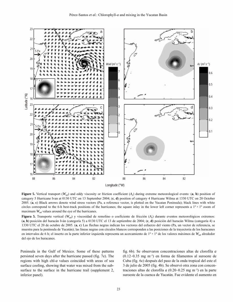
Along the track of Hurricane Ivan (category 5, maximumwind speeds of 68.5 m s–1, maximum wind stress of 15.7 Pa;table 2), the Wad values (fig. 5a) were one order of magnitudegreater (maximum of 8.4 m2 s–1) than those of Az, therebyreversing the relative importance of advective transport com-pared to that during weak or moderate meteorological events.During the hurricane, Az was still high, with maximum valuesof 0.64 m2 s–1 (fig. 5b). This is about three times higher thanthe regional yearly mean (fig. 2), reflecting the mixing powerof hurricanes.

During Hurricane Wilma (category 4), similar windmixing and Ekman pumping were observed. Wad (5.4 m2 s–1)was one order of magnitude higher than Az (0.45 m2 s–1) whenWilma moved through the Yucatan Basin, with maximumspeeds of 57.6 m s–1 and maximum wind stress of 11.1 Pa(fig. 5c, d; table 2). As with Hurricane Ivan, the maximumvalues of Wad and Az were located in an area ~100 ×100 km

and ~300 × 300 km, respectively, around the eye of the hurri-cane (inlays fig. 5a, c).

The DE reached maximum values of 103 m during thepassage of the cold front, 115 m during the easterly tropical

extremos como se observó en la serie de tiempo promedioanual (fig. 2).

Onda tropical del este

Del 3 al 5 de julio de 2005, durante el paso de una ondatropical del este por la cuenca de Yucatán, soplaron vientosfuertes del sureste con una velocidad media de 9.4 m s–1

(tabla 2). El esfuerzo del viento fue máximo a 0.49 Pa(fig. 4c), con una Az de aproximadamente 33 × 10–3 m2 s–1

(fig. 4d). La velocidad vertical advectiva fue hacia arriba enlas partes central y este de la cuenca de Yucatán (fig. 4c), conun transporte vertical máximo (4.8 × 10–3 m2 s–1) mayor quela media anual, pero bajo comparado con Az. Los valoresmáximos se registraron en la parte oeste de la cuenca, entre laisla de Cozumel y el banco Chinchorro.

Sistema de baja presión

Un sistema de baja presión pasó sobre Pinar del Río(oeste de Cuba) el 5 de octubre de 2005 (fig. 4e). Lavelocidad media del viento fue moderada en la mayor partede la región (6.3 m s–1, tabla 2), registrándose los mayoresvalores (18.27 m s–1) al este de la península de Yucatán.Ahí, el esfuerzo del viento presentó un máximo de 0.75 Pa(fig. 4e), lo cual resultó en el valor más alto de Az (45 10–3 m2 s–1) en la categoría de eventos meteorológicos mode-rados (fig. 4f). Las velocidades advectivas verticales fueronfuertemente hacia arriba al sur de 20º N (fig. 4e), con veloci-dades máximas (7.8 10–3 m2 s–1) en la costa.

Table 1. Median of the vertical eddy diffusivity (Kv), the gradient Richardson number (Ri), and the mixed layer depth (MLD) time series (2007to 2009) (MERCATOR output) for the locations off southern Cuba and eastern Yucatan.Tabla 1. Mediana de la serie de tiempo (2007 a 2009) de la difusividad vertical de remolino (Kv), el número de Richardson (Ri) y laprofundidad de la capa de mezcla (MLD) (datos de MERCATOR) para los sitios al sur de Cuba y este de Yucatán.

MedianWinter

(Jan., Feb., Mar.)Spring

(Apr., May, June)Summer

(July, Aug., Sep.)Autumn

(Oct., Nov., Dec.)

Southern Cuba

Kv max. (m2 s–1) 1.0 10–4 5.2 10–5 1.2 10–2 1.7 10–4 2.6 10–5

Kvm (m) 27.3 43.8 14.6 17.1 51.5

Ri min. (m2 s–1) 0.76 1.25 0.22 0.50 2.03

Rim (m) 27.3 43.8 14.6 17.1 51.5

MLD (m) 42.5 78.4 22.4 25.1 59.2

Eastern Yucatan

Kv max. (m2 s–1) 1.6 10–3 1.8 10–4 8.8 10–1 2.7 10–1 1.2 10–4

Kvm (m) 20.0 27.3 10.4 8.7 31.9

Ri min. (m2 s–1) 0.27 0.48 0.13 0.15 0.68

Rim (m) 20.0 27.3 10.4 8.7 31.9

MLD (m) 31.8 49.5 22.1 21.5 40.8

Kvm and Rim represent the depth of the maximum value of Kv max. and Ri min.


21

wave, and 135 m during the low-pressure system. The deep-est DE were observed around the eyes of hurricanes Ivan andWilma, at 505 and 440 m, respectively (figure not shown).Both values were registered to the right side of the eye of thetwo hurricanes. These values were overestimated becausewater column stability was not included in the calculations.

Chlorophyll-a response

Satellite-derived chl-a concentration images collectedduring and after the passage of these synoptic meteorological

Huracanes

A lo largo de la trayectoria del huracán Iván (categoría 5,velocidad máxima del viento de 68.5 m s–1, esfuerzo máximodel viento de 15.7 Pa; tabla 2), los valores de Wad (fig. 5a)fueron un orden de magnitud mayor (máximo de 8.4 m2 s–1)que los de Az, revirtiendo así la importancia relativa del trans-porte advectivo comparado con el observado durante loseventos meteorológicos débiles o moderados. Durante elhuracán, Az aún fue alta, con valores máximos de 0.64 m2 s–1

(fig. 5b); esto es alrededor de tres veces mayor que la media

Longitude (°W)

23

22

21

20

19

18

Latit

ude

(°N

)

23

22

21

20

19

18

23

22

21

20

19

1888 86 84 82 80

0.5

0

1

a b

c d

10

5

20

15

10

5

15

20

25

0

-1

1

2

3

-2

-4

0

2

4

10

30

40

20

e f

88 86 84 82 80

7 Nov 2004

4 Jul 2005

5 Oct 2005

0.2 Pa

0.2 Pa

0.2 Pa

Figure 4. Vertical transport (Wad, grey-shaded with zero black contour line) and vertical eddy viscosity coefficient (Az, grey-shaded), duringmoderate meteorological events: (a, b) cold front (7 November 2004), (c, d) tropical wave (4 July 2005), and (e, f) low-pressure system(5 October 2005). Black arrows in (a), (c), and (e) indicate wind stress vectors (Pa, a reference vector, is plotted on the Yucatan Peninsula).Solid black contour lines in (b), (d), and (f) represent the surface Ekman layer depth (m).

Figura 4. Transporte vertical (Wad, tonos de gris con línea negra de contorno cero) y coeficiente de la viscosidad vertical de remolino(Az, tonos de gris), durante eventos meteorológicos moderados: (a, b) frente frío (7 de noviembre de 2004), (c, d) onda tropical (4 de julio de2005) y (e, f) sistema de baja presión (5 de octubre de 2005). Las flechas negras en (a), (c) y (e) indican vectores del esfuerzo del viento(Pa, un vector de referencia, se muestra para la península de Yucatán). Las líneas negras de contorno en (b), (d) y (f) representan laprofundidad de la capa de Ekman (m).


22

events showed heavy cloud cover. In the days following thepassage of the cold front over the Yucatan Basin, around7 November 2004 (fig. 4a), chl-a concentrations throughoutthe basin rose to mean levels between 0.08 and 0.12 mg m–3

(fig. 6a, b). Maximum concentrations (~0.38 mg m–3) wereobserved in a ~50-km-long chl-a filament that appearedsouth of the San Felipe keys (Gulf of Batabanó, southwestCuba) (fig. 6a). A longer filament of 120 km was observedextending south of Cape San Antonio, Cuba (fig. 6a),advected around a small cyclonic eddy centered about21.5º N, 85º W (white box in fig. 6b). Filaments of high chl-a(0.12–0.35 mg m–3) were observed off the southwest cornerof Cuba (fig. 6c) after the easterly tropical wave movedthrough the region on 3 July 2005 (fig. 4b). Another area withhigh chl-a concentrations (0.20–0.25 mg m–3) was observedin the southwestern Yucatan Basin. Basin-wide increasesin chl-a were evident (0.07–0.12 mg m–3, fig. 6d) afterthe low-pressure system crossed the Yucatan Basin around6 October 2005 (fig. 4c). A filament (~1.4 mg m–3) of~300 km length and 50 km width extended south of SanFelipe Keys (Cuba) to Cayman Island. A shorter filamentwas observed again off Cape San Antonio (western Cuba)during this event.

On 11 September 2004, two days before Hurricane Ivanpassed through the Yucatan Basin, chl-a concentrations werelow (~0.03 mg m–3) (fig. 7a). On 20 September 2004, oneweek after Hurricane Ivan passed over southern Cuba, fila-ments and patches were observed in the center of the YucatanBasin (fig. 7b). Several filaments extended northward, intothe Gulf of Mexico, from the Gulf of Guanahacabibes(western Cuba), and to the east and southwest of Pinos Island(southwestern Cuba, fig. 7b). High concentrations wereobserved on 25 October 2005 (fig. 7d), five days afterHurricane Wilma (fig. 5c) passed through the Yucatan Basin.Along the track of Hurricane Wilma, chl-a concentrationsexceeded 1.0 mg m–3 in the western Yucatan Basin andparticularly in the upwelling area off the northern Yucatan

regional anual (fig. 2), y refleja el poder de mezcla de loshuracanes.

Durante el huracán Wilma (categoría 4), la mezcla cau-sada por el viento y el bombeo de Ekman fueron similares.Wad (5.4 m2 s–1) fue un orden de magnitud mayor que Az

(0.45 m2 s–1) cuando Wilma pasó por la cuenca de Yucatán,con velocidades máximas de 57.6 m s–1 y un esfuerzomáximo del viento de 11.1 Pa (fig. 5c, d; tabla 2). Al igualque el huracán Iván, los valores máximos de Wad y Az seregistraron en un área de ~100 ×100 km y ~300 ×300 km,respectivamente, alrededor del ojo del huracán (insertosfig. 5a, c).

La DE alcanzó valores máximos de 103 m durante elfrente frío, de 115 m durante la onda tropical del este y de135 m durante el sistema de baja presión. La DE más pro-funda se observó alrededor de los ojos de los huracanes Ivány Wilma, a 505 y 440 m, respectivamente (no se muestra lafigura). Ambos valores fueron registrados del lado derechodel ojo de los huracanes. Estos valores fueron sobreestimadosporque no se consideró la estabilidad de la columna de aguaen los cálculos.

Respuesta de la clorofila a

Las imágenes satelitales de la concentración de clorofila aobtenidas durante y después del paso de estos eventos meteo-rológicos mostraron una fuerte nubosidad. En los díasdespués del paso del frente frío sobre la cuenca de Yucatán,alrededor del 7 de noviembre de 2004 (fig. 4a), las concentra-ciones de clorofila a aumentaron a niveles de entre 0.08 y0.12 mg m–3 (fig. 6a, b). Las concentraciones máximas(~0.38 mg m–3) se registraron en un filamento de clorofila ade ~50 km de largo que apareció al sur de los cayos de SanFelipe (golfo de Batabanó, suroeste de Cuba) (fig. 6a). Sedetectó un filamento más largo, de 120 km, al sur de CaboSan Antonio, Cuba (fig. 6a), alrededor de un giro ciclónicopequeño centrado en 21.5º N, 85º W (cuadro blanco en

Table 2. Statistical characteristics of vertical eddy viscosity (Az), vertical advective transport (Wad), and Ekman layer depth (DE) during thepassage of synoptic-scale meteorological events over the Yucatan Basin.Tabla 2. Características estadísticas de la viscosidad vertical de remolino (Az), el transporte vertical advectivo (Wad) y la profundidad de la capade Ekman (DE) durante el paso de eventos meteorológicos de escala sinóptica por la cuenca de Yucatán.

Synoptic eventDate

(d/m/yr)

Meanwindspeed(m s–1)

Meanwindstress(Pa)

Az

(m2 s–1)

Wad

(m2 s–1)DE

(m)

Mean Max. Mean Max. Mean Max.

Cold front 07/11/2004 8.7 0.12 10.7 10–3 23.1 10–3 0.18 10–3 1.8 10–3 63 103

Tropical wave 04/07/2005 9.4 0.15 12.9 10–3 33.0 10–3 0.35 10–3 4.8 10–3 67 115

Low-pressure system 05/10/2005 6.3 0.07 6.5 10–3 45.5 10–3 0.20 10–3 7.8 10–3 46 135

Hurricane Ivan 13/09/2004 68.5 15.70 0.058 0.64 0.018 8.4 138 506

Hurricane Wilma 20/10/2005 57.6 11.10 0.053 0.45 0.017 5.4 140 440


23

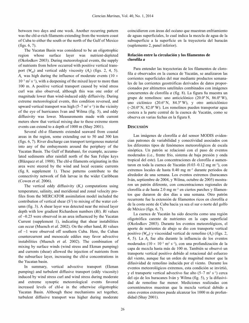
Peninsula in the Gulf of Mexico. Some of these patternspersisted seven days after the hurricane passed (fig. 7e). Theregions with high chl-a values coincided with areas of seasurface cooling, showing that water was mixed from the sub-surface to the surface in the hurricane trail (supplement 2,inferior panel).

fig. 6b). Se observaron concentraciones altas de clorofila a(0.12–0.35 mg m–3) en forma de filamentos al suroeste deCuba (fig. 6c) después del paso de la onda tropical del este el3 de julio de 2005 (fig. 4b). Se observó otra zona con concen-traciones altas de clorofila a (0.20–0.25 mg m–3) en la partesuroeste de la cuenca de Yucatán. Fue evidente el aumento en

0.1

0.2

0.3

0.4

Az (m s ) 2 1¯

0.5

0.6

0

1

2

3

Wad (m s ) 2 1¯

4

5

6

7

Longitude (°W)

23

22

21

20

19

18

88 86 84 82

17

16

23

22

21

20

19

18

17

16

88 86 84 82

Latit

ude

(°N

)

a b

c d

1° x 1°

1° x 1°

5 Pa

5 Pa

Figure 5. Vertical transport (Wad) and eddy viscosity or friction coefficient (Az) during extreme meteorological events: (a, b) position ofcategory 5 Hurricane Ivan at 0130 UTC on 13 September 2004; (c, d) position of category 4 Hurricane Wilma at 1330 UTC on 20 October2005. (a, c) Black arrows denote wind stress vectors (Pa, a reference vector, is plotted on the Yucatan Peninsula); black lines with whitecircles correspond to the 6-h best-track positions of the hurricanes; the square inlay in the lower left corner represents a 1º × 1º zoom ofmaximum Wad values around the eye of the hurricanes.

Figura 5. Transporte vertical (Wad) y viscosidad de remolino o coeficiente de fricción (Az) durante eventos meteorológicos extremos:(a, b) posición del huracán Iván (categoría 5) a 0130 UTC el 13 de septiembre de 2004; (c, d) posición del huracán Wilma (categoría 4) a1330 UTC el 20 de octubre de 2005. (a, c) Las flechas negras indican los vectores del esfuerzo del viento (Pa, un vector de referencia, semuestra para la península de Yucatán); las líneas negras con círculos blancos corresponden a las posiciones de la trayectoria de los huracanesen intervalos de 6 h; el inserto en la parte inferior izquierda representa un acercamiento de 1º × 1º de los valores máximos de Wad alrededordel ojo de los huracanes.


24

Relationship between circulation and chlorophyll-a filaments

Sea surface currents were analyzed in order to understandthe trajectories of chl-a filaments observed in the YucatanBasin using weekly geostrophic current products derivedfrom satellite altimeter data merged with concurrent chl-aimages (fig. 8). Figure 8a shows a group of eddies: one anti-cyclonic (20.0º N, 86.0º W), one cyclonic (20.6º N, 84.3º W),and another anti-cyclonic (~20.0º N, 82.0º W). These eddiescan advect coastal water into the central Yucatan Basin, asobserved on multiple dates in figure 8.

DISCUSSION

The MODIS chl-a images highlight patterns of variabilityand connectivity associated with different types of meteoro-logical events. One pattern was related to the passage ofmoderate synoptic events (i.e., cold front, low-pressure

las concentraciones de clorofila a (0.07–0.12 mg m–3, fig. 6d)en toda la cuenca de Yucatán después del paso del sistema debaja presión alrededor del 6 de octubre de 2005 (fig. 4c). Unfilamento (~1.4 mg m–3) de ~300 km de largo y 50 km deancho se extendió del sur de los cayos de San Felipe (Cuba) ala isla Caimán. Durante este evento, se volvió a observar unfilamento más corto en frente de cabo San Antonio (oeste deCuba).

El 11 de septiembre de 2004, dos días antes del paso delhuracán Iván por la cuenca de Yucatán, las concentracionesde clorofila a fueron bajas (~0.03 mg m–3) (fig. 7a). El 20 deseptiembre de 2004, una semana después del paso delhuracán Iván por el sur de Cuba, se observaron filamentos yparches en la parte central de la cuenca de Yucatán (fig. 7b).Varios filamentos se extendieron hacia el norte, hasta el golfode México, desde el golfo de Guanahacabibes (oeste deCuba), y hacia el este y suroeste de la isla de Pinos (suroestede Cuba, fig. 7b). Se observaron concentraciones altas el25 de octubre de 2005 (fig. 7d), cinco días después del paso

22

20

18

22

20

1888 86 84 82 80 88 86 84 82 80

Longitude (°W)

Latit

ude

(°N

)

0.03 0.10 0.20 0.50 1.00 1.50Chl- (mg m )a ¯3

Figure 6. MODIS chlorophyll-a (chl-a) images (a, b) after the passage of a cold front, (c) after the passage of an easterly tropical wave, and(d) after the passage of a low-pressure system through the Yucatan Basin. Black regions represent no data (clouds). White squares indicate thelocation where mesoscale eddies were observed.

Figura 6. Imágenes de MODIS de la concentración de clorofila a (chl-a) después del paso de (a, b) un frente frío, (c) una onda tropical deleste y (d) un sistema de baja presión por la cuenca de Yucatán. Las regiones negras indican que no hay datos (nubosidad). Los cuadrosblancos señalan las zonas donde se observaron remolinos de mesoescala.


25

system, and easterly tropical wave). Increased chl-a concen-trations (0.03–0.12 mg m–3) were observed throughout theYucatan Basin, with local extremes up to 0.40 mg m–3 forperiods of about a week. Extreme events (hurricanes Ivan,September 2004, and Wilma, October 2005) showed adifferent pattern, with high regional chl-a concentrations upto 2.0 mg m–3 in concentrated patches and filaments lasting

del huracán Wilma (fig. 5c) por la cuenca de Yucatán. A lolargo de la trayectoria de Wilma, las concentraciones declorofila a excedieron 1.0 mg m–3 en la parte oeste de lacuenca y especialmente en la zona de surgencias al norte dela península de Yucatán en el golfo de México. Algunos deestos patrones persistieron siete días después del paso delhuracán (fig. 7e). Las regiones con valores altos de clorofila a

22

20

22

20

1888 86 84 82 80

Longitude (°W)

Latit

ude

(°N

)

18

88 86 84 82 80

88 86 84 82 80

22

20

18

0.03 0.10 0.20 0.50 1.00 1.50Chl- (mg m )a ¯3

Figure 7. MODIS chlorophyll a (chl-a) images (a) before and (b) after the passage of Hurricane Ivan, and (c) before and (d, e) after thepassage of Hurricane Wilma through the Yucatan Basin. Black regions represent no data (clouds).

Figura 7. Imágenes de MODIS de la concentración de clorofila a (chl-a) (a) antes y (b) después del paso del huracán Iván, y (c) antes y(d, e) después del paso del huracán Wilma por la cuenca de Yucatán. Las regiones negras indican que no hay datos (nubosidad).


26

between two days and one week. Another recurring patternwas the chl-a-rich filaments extending from the western coastof Cuba to either the south or the north of the Gulf of Mexico(figs. 6, 7).

The Yucatan Basin was considered to be an oligotrophicregion whose surface layer was nutrient-depleted(Okolodkov 2003). During meteorological events, the supplyof nutrients from below occurred with positive vertical trans-port (Wad) and vertical eddy viscosity (Az) (figs. 2, 4, 5).Az was high during the influence of moderate events (10 10–3 m2 s–1), with a deepening of the mixed layer to more than100 m. A positive vertical transport caused by wind stresscurl was also observed, although this was one order ofmagnitude lower than wind-induced eddy diffusivity. Duringextreme meteorological events, this condition reversed, andupward vertical transport was high (5–7 m2 s–1) in the vicinityof the eye of hurricanes Ivan and Wilma (fig. 5), and eddydiffusivity was lower. Measurements made with currentmeters show that vertical mixing due to these extreme stormevents can extend to a depth of 1000 m (Shay 2001).

Several chl-a filaments extended seaward from coastalareas in the region, some extending out to 50 and 300 km(figs. 6, 7). River discharge can transport terrigenous materialinto any of the embayments around the periphery of theYucatan Basin. The Gulf of Batabanó, for example, accumu-lated sediments after rainfall north of the San Felipe keys(Blázquez et al. 1988). The chl-a filaments originating in thisarea were steered by the wind and local oceanic currents(fig. 8, supplement 1). These patterns contribute to theconnectivity network of fish larvae in the wider Caribbean(Cowen et al. 2006).

The vertical eddy diffusivity (Kv) computations usingtemperature, salinity, and meridional and zonal velocity pro-files from the MERCATOR assimilation model included thecontribution of vertical shear (S2) to mixing of the water col-umn (fig. 3). A shear layer was detected near the mixed layerdepth with low gradient Richardson numbers (Ri). Ri valuesof ~0.25 were observed in an area influenced by the YucatanCurrent (supplement 1), indicating that shear instabilitiescan occur (Muench et al. 2002). On the other hand, Ri valuesof ~1 were observed off southern Cuba. Here, the Cubancountercurrent and mesoecale eddies may favor advectiveinstabilities (Muench et al. 2002). The combination ofmixing by surface winds (wind stress and Ekman pumping)and currents (shear) allowed the injection of nutrients fromthe subsurface layer, increasing the chl-a concentrations inthe Yucatan basin.

In summary, vertical advective transport (Ekmanpumping) and turbulent diffusive transport (eddy viscosity)induced by wind stress curl and wind stress during moderateand extreme synoptic meteorological events favoredincreased levels of chl-a in the otherwise oligotrophicYucatan Basin. Although these mechanisms act together,turbulent diffusive transport was higher during moderate

coincidieron con áreas del océano que muestran enfriamientode aguas superficiales, lo cual indica la mezcla de agua de lasubsuperficie a la superficie en la trayectoria del huracán(suplemento 2, panel inferior).

Relación entre la circulación y los filamentos declorofila a

Para entender las trayectorias de los filamentos de cloro-fila a observados en la cuenca de Yucatán, se analizaron lascorrientes superficiales del mar mediante productos semana-les de las corrientes geostróficas derivados de datos propor-cionados por altímetros satelitales combinados con imágenesconcurrentes de clorofila a (fig. 8). La figura 8a muestra ungrupo de remolinos: uno anticiclónico (20.0º N, 86.0º W),uno ciclónico (20.6º N, 84.3º W), y otro anticiclónico(~20.0º N, 82.0º W). Los remolinos pueden transportar aguacostera a la parte central de la cuenca de Yucatán, como seobserva en varias fechas en la figura 8.

DISCUSIÓN

Las imágenes de clorofila a del sensor MODIS eviden-cian patrones de variabilidad y conectividad asociados conlos diferentes tipos de fenómenos meteorológicos de escalasinóptica. Un patrón se relacionó con el paso de eventosmoderados (i.e., frente frío, sistema de baja presión y ondatropical del este). Las concentraciones de clorofila a aumen-taron en toda la cuenca de Yucatán (0.03–0.12 mg m–3), conextremos locales de hasta 0.40 mg m–3 durante periodos dealrededor de una semana. Los eventos extremos (huracanesIván, septiembre de 2004, y Wilma, octubre de 2005) mostra-ron un patrón diferente, con concentraciones regionales declorofila a de hasta 2.0 mg m–3 en ciertos parches y filamen-tos que duraron de dos días a una semana. Otro patrónrecurrente fue la extensión de filamentos ricos en clorofila ade la costa oeste de Cuba hacia ya sea el sur o norte del golfode México (figs. 6, 7).

La cuenca de Yucatán ha sido descrita como una regiónoligotrófica carente de nutrientes en la capa superficial(Okolodkov 2003). Durante los eventos meteorológicos, elaporte de nutrientes de abajo se dio con transporte verticalpositivo (Wad) y viscosidad vertical de remolino (Az) (figs. 2,4, 5). La Az fue alta durante la influencia de los eventosmoderados (10 10–3 m2 s–1), con una profundización de lacapa de mezcla hasta más de 100 m. También se observó untransporte vertical positivo debido al rotacional del esfuerzodel viento, aunque fue un orden de magnitud menor que ladifusividad de remolino inducida por el viento. Durante loseventos meteorológicos extremos, esta condición se invirtió,y el transporte vertical advectivo fue alto (5–7 m2 s–1) cercadel ojo de los huracanes Iván y Wilma (fig. 5), y la difusivi-dad de remolino fue menor. Mediciones realizadas concorrentómetros muestran que la mezcla vertical debido aestos eventos extremos puede alcanzar los 1000 m de profun-didad (Shay 2001).


27

events, whereas vertical advective transport became domi-nant during extreme events. Low Ri values were observed onthe western side of the Yucatan Basin due to the influenceand variability of the Yucatan Current, suggesting thatvertical shear instabilities in the flow can enhance mixingin the water column. The three-dimensional data of theMERCATOR assimilation model proved to be a helpful toolto study the temporal and spatial variability of mixing pro-cesses in the Yucatan Basin.

The presence of high chl-a concentrations in the form offilaments after the passage of synoptic-scale meteorologicalevents, combined with increased precipitation on the Cubanisland, demonstrated the importance of terrestrial nutrientsources, including inorganic fertilizers, for phytoplanktonblooms in the Gulf of Batabanó, Cuba. The direction andmagnitude of the ocean currents determined the dispersionand the trajectories of these filaments, contributing to theconnectivity in the northwestern Caribbean Sea.

Varios filamentos de clorofila a se extendieron de laszonas costeras hacia mar adentro, algunos por más de 50 y300 km (figs. 6, 7). Las descargas de ríos pueden transportarmaterial terrígeno a cualquier bahía en la periferia de lacuenca de Yucatán. El golfo de Batabanó, por ejemplo,acumuló sedimentos después de que lloviera al norte de loscayos de San Felipe (Blázquez et al. 1988). Los filamentos declorofila a que se originaron en esta zona fueron dirigidospor el viento y las corrientes oceánicas locales (fig. 8, suple-mento 1). Estos patrones contribuyen a la red de conectividadde las larvas de peces en todo el Caribe (Cowen et al. 2006).

Los cálculos de la difusividad vertical de remolino (Kv)con datos de temperatura, salinidad y los perfiles develocidad zonal y meridional del modelo de asimilaciónMERCATOR incluyeron la contribución de la cizalladuravertical (S2) a la mezcla de la columna de agua (fig. 3). Sedetectó una capa de cizalladura cerca de la profundidad de lacapa de mezcla con números de Richardson (Ri) bajos. Seobservaron valores de Ri de ~0.25 en la zona influenciada por

23

22

21

20

19

18

Latit

ude

(°N

)

23

22

21

20

19

18

Longitude (°W)-88 -87 -86 -85 -84 -83 -82 -81 -80

a b

c d

-88 -87 -86 -85 -84 -83 -82 -81 -80

0.06 0.08 0.1 0.2 0.3 0.4 0.5

Figure 8. MODIS chlorophyll a (chl-a) images after the passage of synoptic-scale meteorological events and corresponding weekly meangeostrophic currents (black arrows) from the AVISO altimeter. (a) Cold front (13 November 2004), (b) easterly tropical wave (5 July 2005),(c) low-pressure system (11 October 2005), and (d) Hurricane Wilma (27 October 2005).Figura 8. Imágenes de MODIS de las concentraciones de clorofila a (chl-a) después del paso de eventos meteorológicos de escala sinópticay las correspondientes corrientes geostróficas semanales promedio (flechas negras) del altímetro AVISO. (a) Frente frío (13 de noviembre de2004), (b) onda tropical del este (5 de julio de 2005), (c) sistema de baja presión (11 de octubre de 2005) y (d) huracán Wilma (27 de octubrede 2005).


28

ACKNOWLEDGMENTS

Thanks are due to the National Commission for Scientificand Technological Research (CONICYT, Chile) forproviding a doctorate scholarship for IPS (2006330027-6) tostudy at the University of Concepción, Chile, and to theMECESUP Program for supporting a research stay atAOML-NOAA, Miami, University of South Florida andUniversity of Florida. AVL acknowledges support from theNational Science Foundation (project OCE-0825876). FMKreceived support from NASA grants NNX09AV24G andNNX08AL06G. The authors also thank CONICYT-FONDECYT (grant 3120038), COPAS Sur Austral (grantPFB 31/2007), and the anonymous reviewers.

REFERENCES

Babin SM, Carton JA, Dickey TD, Wiggert JD. 2004. Satelliteevidence of hurricane-induced phytoplankton blooms in anoceanic desert. J. Geophys. Res. 109(C3).http://dx.doi.org/10.1029/2003jc001938

Blázquez L, Rodríguez JP, Rosabal I, Calderón R. 1988. Medicionesde corrientes en el Golfo de Batabanó. Rep. Invest. Inst.Oceanol. Acad. Cienc. Cuba 14: 1–36.

Centurioni LR, Niiler PP. 2003. On the surface currents of theCaribbean Sea. Geophys. Res. Lett. 30(6).http://dx.doi.org/10.1029/2002gl016231

Cowen RK, Paris CB, Srinivasan A. 2006. Scaling of connectivityin marine populations. Science 311(5760): 522–527.http://dx.doi.org/10.1126/science.1122039

Donelan MA, Haus BK, Reul N, Plant WJ, Stiassnie M, Graber HC,Brown OB, Saltzman ES. 2004. On the limiting aerodynamicroughness of the ocean in very strong winds. Geophys. Res.Lett. 31(18).http://dx.doi.org/10.1029/2004gl019460

González NM, Müller-Karger FE, Estrada SC, Pérez De Los ReyesR, Del Río IV, Pérez PC, Arenal IM. 2000. Near-surfacephytoplankton distribution in the western Intra-Americas Sea:The influence of El Niño and weather events. J. Geophys. Res.105(C6): 14029–14043.http://dx.doi.org/10.1029/2000jc900017

González PC. 1999. Climatología de los frentes fríos que hanafectado a Cuba desde 1916–1917 hasta 1996–1997. Rev. Cub.Meteorol. 6: 15–19.

Johns WE, Townsend TL, Fratantoni DM, Wilson WD. 2002. Onthe Atlantic inflow to the Caribbean Sea. Deep-Sea Res. I 49:211–243.http://dx.doi.org/10.1016/S0967-0637(01)00041-3

Jouanno J, Sheinbaum J, Barnier B, Molines JM, Debreu L, LemarieF. 2008. The mesoscale variability in the Caribbean Sea. Part I:Simulations and characteristics with an embedded model. OceanModel. 23: 82–101.http://dx.doi.org/10.1016/j.ocemod.2008.04.002

Letelier RM, Abbott MR. 1996. An analysis of chlorophyllfluorescence algorithms for the moderate resolution imagingspectrometer (MODIS). Remote Sens. Environ. 58: 215–223.http://dx.doi.org/10.1016/S0034-4257(96)00073-9

Locarnini RA, Mishonov AV, Antonov JI, Boyer TP, Garcia HE,Baranova OK, Zweng MM, Johnson DR. 2010. World OceanAtlas 2009. Volume 1: Temperature. In: Levitus S (ed.), NOAAAtlas NESDIS 68, US Government Printing Office, WashingtonDC, 184 pp.

la corriente de Yucatán (suplemento 1), lo que indica quepueden suceder inestabilidades de cizalladura (Muench et al.2002). Por otro lado, se observaron valores de Ri de ~1 al surde Cuba. Aquí, la contracorriente cubana y los remolinos demesoescala pueden favorecer inestabilidades advectivas(Muench et al. 2002). La combinación de mezcla por vientossuperficiales (esfuerzo del viento y bombeo de Ekman) ycorrientes (cizalladura) permitió la inyección de nutrientes dela capa subsuperficial, incrementando las concentraciones declorofila a en la cuenca de Yucatán.

En resumen, el transporte vertical advectivo (bombeo deEkman) y el transporte difusivo turbulento (viscosidad deremolino), inducidos por el esfuerzo del viento y su rotacio-nal durante eventos meteorológicos moderados y extremos deescala sinóptica, favorecieron el incremento de los niveles declorofila a en la oligotrófica cuenca de Yucatán. Aunqueestos mecanismos actúan en conjunto, el transporte difusivoturbulento fue mayor durante los eventos moderados, mien-tras que el transporte vertical advectivo dominó durante loseventos extremos. Se registraron valores de Ri bajos dellado oeste de la cuenca de Yucatán debido a la influencia yvariabilidad de la corriente de Yucatán, lo que sugiere queinestabilidades de cizalladura vertical en el flujo puedenincrementar la mezcla en la columna de agua. Los datostridimensionales del modelo de asimilación MERCATORresultaron ser una herramiento útil para estudiar la variabili-dad temporal y espacial de los procesos de mezcla en lacuenca de Yucatán.

La presencia de concentraciones altas de clorofila a enforma de filamentos después del paso de eventos meteoroló-gicos de escala sinóptica, en conjunto con un incremento dela precipitación en la isla de Cuba, mostró la importancia delas fuentes terrestres de nutrientes, incluyendo los fertilizan-tes inorgánicos, para los afloramientos de fitoplancton en elgolfo de Batabanó, Cuba. La dirección y magnitud de lascorrientes oceánicas determinó la dispersión y las trayecto-rias de estos filamentos, contribuyendo a la conectividad enel mar Caribe noroccidental.

AGRADECIMIENTOS

Se agradece a la Comisión Nacional de InvestigaciónCientífica y Tecnológica (CONICYT, Chile) la beca otorgadaa IPS (2006330027-6) para realizar estudios doctorales en laUniversidad de Concepción, Chile, y al programa MECESUPsu apoyo para una estancia en AOML-NOAA, Miami,Universidad del Sur de Florida y Universidad de Florida.AVL agradece el apoyo de la Fundación Nacional de laCiencia (NSF) de los Estados Unidos (proyecto OCE-0825876). FMK reconoce el apoyo recibido de la NASA(NNX09AV24G y NNX08AL06G). También se agradece aCONICYT-FONDECYT (proyecto 3120038) y COPAS SurAustral (proyecto PFB 31/2007), así como a los revisoresanónimos.

Traducido al español por Christine Harris.


29

Lorbacher K, Dommenget D, Niiler PP, Kohl A. 2006. Ocean mixedlayer depth: A subsurface proxy of ocean-atmospherevariability. J. Geophys. Res. 111(C7).http://dx.doi.org/10.1029/2003jc002157

Marcotte D. 1991. Cokriging with Matlab. Comput. Geosci. 17:1265–1280.http://dx.doi.org/10.1016/0098-3004(91)90028-C

McClain CR. 2009. A decade of satellite ocean color observations.Annu. Rev. Mar. Sci. 1: 19–42.http://dx.doi.org/10.1146/annurev.marine.010908.163650

Muench RD, Padman L, Howard SL, Fahrbach E. 2002. Upperocean diapycnal mixing in the northwestern Weddell Sea. Deep-Sea Res. II 49: 4843–4861.http://dx.doi.org/10.1016/S0967-0645(02)00162-5

Müller-Karger FE, Walsh JJ, Evans RH, Meyers MB. 1991. On theseasonal phytoplankton concentration and sea surfacetemperature cycles of the Gulf of Mexico as determined bysatellites. J. Geophys. Res. 96(C7): 12645–12665.http://dx.doi.org/10.1029/91jc00787

Okolodkov YB. 2003. A review of Russian plankton research in theGulf of Mexico and the Caribbean Sea in the 1960–1980s.Hidrobiológica 13: 207–221.http://www.redalyc.org/articulo.oa?id=57813306

Peláez JA, McGowan J. 1986. Phytoplankton pigment patterns inthe California Current as determined by satellite. Limnol.Oceanogr. 31: 927–950.http://dx.doi.org/10.4319/lo.1986.31.5.0927

Pérez-Santos I, Schneider W, Sobarzo M, Montoya-Sánchez R,Valle-Levinson A, Garcés-Vargas J. 2010. Surface windvariability and its implications for the Yucatan Basin-CaribbeanSea dynamics. J. Geophys. Res. 115.http://dx.doi.org/10.1029/2010jc006292

Pond S, Pickard GL. 1983. Introductory Dynamical Oceanography.Pergamon Press, Oxford, 329 pp.

Rodríguez-Santana A, Pelegrí JL, Sangra P, Marrero-Díaz A. 1999.Diapycnal mixing in Gulf Stream meanders. J. Geophys. Res.104(C11): 25891–25912.http://dx.doi.org/10.1029/1999jc900219

Romanou A, Chassignet EP, Sturges W. 2004. Gulf of Mexicocirculation within a high-resolution numerical simulation of theNorth Atlantic Ocean. J. Geophys. Res. 109(C1).http://dx.doi.org/10.1029/2003jc001770

Shay LK. 2001. Upper ocean structure: Response to strong forcingevents. In: Steele J, Thorpe S, Turekian K (eds.), Encyclopediaof Ocean Science. Academic Press, London, pp. 3100–3114.

Smith RL. 1968. Upwelling. In: Barnes H (ed.), Oceanography andMarine Biology. An Annual Review. George Allen and Unwin,Ltd., London, pp. 11–46.

Stewart RH. 2008. Introduction to Physical Oceanography.Department of Oceanography, Texas A & M University,College Station, Texas, 345 pp.

Wang C, Enfield DB. 2001. The tropical Western Hemisphere warmpool. Geophys. Res. Lett. 28: 1635–1638.http://dx.doi.org/10.1029/2000gl011763

Wang C, Lee SK. 2007. Atlantic warm pool, Caribbean low-leveljet, and their potential impact on Atlantic hurricanes. Geophys.Res. Lett. 34(2).http://dx.doi.org/10.1029/2006gl028579

Yelland M, Taylor PK. 1996. Wind stress measurements from theopen ocean. J. Phys. Oceanogr. 26: 541–558.http://dx.doi.org/10.1175/1520-0485(1996)026<0541:Wsmfto>2.0.Co;2

Received June 2013,accepted December 2013.

Supplementary material:

In order to provide evidence that the MERCATOR data represented the circulation patterns of the Yucatan Basin, CaribbeanSea, a surface map is presented in supplement 1. The results obtained with the MERCATOR model match the general circulationshown by ocean models and in situ data published for this region (e.g., Johns et al. 2002, Centurioni and Niiler 2003, Romanouet al. 2004, Jouanno et al. 2008; see text for references). Also, to confirm that deeper cold water was mixed into the surface layerduring hurricane passage, sea surface temperature (SST) maps during the passage of hurricanes Ivan and Wilma are included assupplement 2. These maps are based on SST images reconstructed by optimum interpolation from the combined AdvancedMicrowave Scanning Radiometer and Advanced Very High Resolution Radiometer. In addition, to estimate from which depththese colder waters stem, we include vertical climatological monthly mean temperature profiles for the months corresponding tothe passage of the hurricanes. Temperature data were taken from Locarnini et al. (2010).

Para proporcionar evidencia de que los datos del modelo MERCATOR representan los patrones de circulación de la cuencade Yucatán, mar Caribe, en el suplemento 1 se presenta un mapa superficial. Los resultados obtenidos con este modelo coincidencon la circulación general que muestran modelos oceánicos y datos in situ publicados para esta región (e.g., Johns et al. 2002,Centurioni y Niiler 2003, Romanou et al. 2004, Jouanno et al. 2008; ver el texto para las referencias). Además, para confirmarque se mezcló agua profunda más fría con agua superficial durante el paso de los huracanes, se incluyen mapas de la temperaturasuperficial del mar (TSM) durante el paso de los huracanes Iván y Wilma (suplemento 2). Estos mapas se basan en imágenes deTSM reconstruidas mediante interpolación óptima de los sensores Advanced Microwave Scanning Radiometer y Advanced VeryHigh Resolution Radiometer. Para estimar la profundidad de donde provinieron estas aguas frías, se incluyen perfiles verticalesclimatológicos de temperatura media mensual para los meses que correspondieron al paso de los huracanes. Los datos de temper-atura fueron tomados de Locarnini et al. (2010).


30

26

a bMercator

(1/6°)Altimetry

(1/3°)

24

22

20

18

16

Latit

ude

(°N

)

Longitude (°W)88 86 84 82 80 88 86 84 82 80

0.2 0.4 0.6 0.8 1.0

(m sVelocity ¯1)

Supplement 1. Long-term mean of the surface geostrophic current systems in the Caribbean Sea and Gulf of Mexico from (a) MERCATORand (b) AVISO data, during 2007–2009. Color contours represent the velocity field and vectors the direction of the currents. Abbreviations inpanel (a): CC, Caribbean Current; YC, Yucatan Current; LC, Loop Current; FC, Florida Current; and CCC, Cuban Countercurrent. Suplemento 1. Promedio a largo plazo de los sistemas de corrientes geostróficas superficiales en el mar Caribe y el golfo de México a partirde datos de (a) MERCATOR y (b) AVISO, durante el periodo de 2007 a 2009. Los contornos de color representan el campo de velocididad ylos vectors la dirección de las corrientes. Siglas en (a): CC, corriente del Caribe; YC, corriente de Yucatán; LC, corriente de Lazo; FC,corriente de Florida; y CCC, contracorriente cubana.


31

24

23

22

21

16

17

20

18

Hurricane Ivan (14 Sep 2004)0

Dep

th (m

)

200

400

600

800

1000

WOA-09 (September)Day 15

Day 14

20.5 /83.5°W°N

0

200

400

600

800

1000

18.5 /85.5°W°N

WOA-09 (October)

Temperature (°C)5 10 15 20 25 30

Longitude (°W)

88 86 84 82

24

23

22

21

16

17

20

18

Hurricane Wilma (22 Oct 2005)

80

Latit

ude

(°N

)

Day 24

Day 23

Day 22

Sea surface temperature (°C)

26 27 28 29 30 31

Supplement 2. (Left) Sea surface temperature during the passage (bold line) of hurricanes Ivan (September 2004) and Wilma (October 2005)through the Yucatan Basin. (Right) Monthly climatological temperature profiles at 20.5° N/83.5° W during September and at 18.5º N/85.5º Wduring October.Suplemento 2. (Izquierda) Temperatura superficial del mar durante el paso (línea negra) de los huracanes Iván (septiembre de 2004) y Wilma(octubre de 2005) por la cuenca de Yucatán. (Derecha) Perfiles mensuales climatológicos de temperatura a 20.5° N/83.5° W duranteseptiembre y a 18.5º N/85.5º W durante octubre.

Documents

Chlorophyll-a patterns and mixing processes in the … · Las imágenes diarias del sensor MODIS a bordo del satélite Aqua permitieron identificar los patrones superficiales de la