Computational Statistics and Data Analysis 52 (2008) 4243–4252www.elsevier.com/locate/csda

Chisquare as a rotation criterion in factor analysisLeo Knusel

Department of Statistics, University of Munich, D-80539 Munich, Germany

Received 6 November 2006; received in revised form 25 January 2008; accepted 25 January 2008Available online 6 February 2008

Abstract

The rotation problem in factor analysis consists in finding an orthogonal transformation of the initial factor loadings so thatthe rotated loadings have a simple structure that can be easily interpreted. The most popular orthogonal transformations are thequartimax and varimax procedures with Kaiser normalization. A classical chisquare contingency measure is proposed as a rotationcriterion. It is claimed that this is a very natural criterion, not only for rotations but also for oblique transformations, that is not tobe found in our popular statistical packages up to now.c© 2008 Elsevier B.V. All rights reserved.

1. Introduction and summary

The classical model of factor analysis (cf. Lawley and Maxwell (1971)) is given by

x = 3f + v, (1)

where x = (x1, . . . , x p)T is the vector of the observed variables, f = ( f1, . . . , fk)

T the vector of the latent commonfactors and v = (v1, . . . , vp)

T the vector of the latent specific factors. The matrix 3 = (λir ) = (p × k) is the socalled loading matrix. It is assumed that the variables x1, . . . , x p are standardized so that E(xi ) = 0 and Var(xi ) = 1for i = 1, . . . , p. Furthermore we assume that all common and specific factors are uncorrelated and that the commonfactors are standardized; then the covariance matrix Σ = (p × p) of x is given by

Σ = 33T+ V, (2)

where V = (p × p) is a diagonal matrix with vi i = var(vi ). If 3 is replaced by 3 = 3R, where R = (k × k) is

an arbitrary orthogonal matrix (rotation matrix), then 33T

= 3RRT3T= 33T and so Eq. (2) remains unchanged,

and also the factor model (1) remains essentially unchanged as f = RTf is again a vector of standardized uncorrelatedcommon factors and thus 3 f = 3RRTf = 3f. So the loading matrix 3 is not uniquely fixed (not identifiable) by thefactor model. But note that

var(xi ) = ci + var(vi ) with ci =

k∑r=1

λ2ir ,

and as a diagonal element of 33T the term ci remains unchanged under any orthogonal transformation of the loadingmatrix; ci is called the communality of the variable xi . The indeterminacy of the loading matrix can be used to find a

E-mail address: knuesel@stat.uni-muenchen.de.

0167-9473/$ - see front matter c© 2008 Elsevier B.V. All rights reserved.doi:10.1016/j.csda.2008.01.021

4244 L. Knusel / Computational Statistics and Data Analysis 52 (2008) 4243–4252

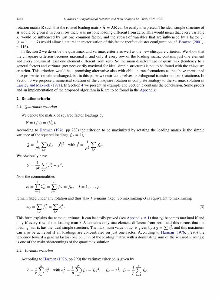
rotation matrix R such that the rotated loading matrix 3 = 3R can be easily interpreted. The ideal simple structure of3 would be given if in every row there was just one loading different from zero. This would mean that every variablexi would be influenced by just one common factor, and the subset of variables that are influenced by a factor fr(r = 1, . . . , k) would allow a natural characterization of this factor (perfect cluster configuration; cf. Browne (2001),p. 116).

In Section 2 we describe the quartimax and varimax criteria as well as the new chisquare criterion. We show thatthe chisquare criterion becomes maximal if and only if every row of the loading matrix contains just one elementand every column at least one element different from zero. So the main disadvantage of quartimax (tendency to ageneral factor) and varimax (not necessarily maximal for ideal simple structure) is not to be found with the chisquarecriterion. This criterion would be a promising alternative also with oblique transformations as the above mentionednice properties remain unchanged, but in this paper we restrict ourselves to orthogonal transformations (rotations). InSection 3 we propose a numerical solution of the chisquare rotation in complete analogy to the varimax solution inLawley and Maxwell (1971). In Section 4 we present an example and Section 5 contains the conclusion. Some proofsand an implementation of the proposed algorithm in R are to be found in the Appendix.

2. Rotation criteria

2.1. Quartimax criterion

We denote the matrix of squared factor loadings by

F = ( fir ) = (λ2ir ).

According to Harman (1976, pp 283) the criterion to be maximized by rotating the loading matrix is the simplevariance of the squared loadings fir = λ2

ir :

Q =1pk

∑i,r

( fir − f )2 with f =1pk

∑i,r

fir .

We obviously have

Q =1pk

∑i,r

f 2ir − f 2.

Now the communalities

ci =

k∑r=1

λ2ir =

k∑r=1

fir = fi•, i = 1, . . . , p,

remain fixed under any rotation and thus also f remains fixed. So maximizing Q is equivalent to maximizing

xQ =

∑i,r

f 2ir =

∑i,r

λ4ir . (3)

This form explains the name quartimax. It can be easily proved (see Appendix A.1) that xQ becomes maximal if andonly if every row of the loading matrix 3 contains only one element different from zero, and this means that theloading matrix has the ideal simple structure. The maximum value of xQ is given by xQ =

∑c2

i , and this maximumcan also be achieved if all loadings are concentrated on just one factor. According to Harman (1976, p.290) thetendency toward a general factor (one column of the loading matrix with a dominating sum of the squared loadings)is one of the main shortcomings of the quartimax solution.

2.2. Varimax criterion

According to Harman (1976, pp 290) the varimax criterion is given by

V =1k

k∑r=1

σ 2r with σ 2

r =1p

p∑i=1

( fir − fr )2, fir = λ2

ir , fr =1p

p∑i=1

fir .

L. Knusel / Computational Statistics and Data Analysis 52 (2008) 4243–4252 4245

Here σ 2r is the variance of the squared loadings in column r . We obviously have

V =1pk

k∑r=1

(p∑

i=1

f 2ir − p f 2

r

)=

1pk

k∑r=1

(p∑

i=1

f 2ir − d2

r /p

)with dr = p fr = f•r =

p∑i=1

fir =

p∑i=1

λ2ir .

So maximizing V is equivalent to maximizing

xV =

k∑r=1

(p∑

i=1

f 2ir − d2

r /p

)= xQ −

1p

k∑r=1

d2r . (4)

The varimax criterion becomes maximal if xQ takes on its maximum and if∑

d2r takes on its minimum which

is the case if all column sums d1, . . . , dk are equal (see Appendix A.2). The example below shows that for thevarimax criterion to become maximal it is not enough that the loading matrix has an ideal simple structure. Thevarimax solution shows a tendency toward factors with equal sums d1, . . . , dk , whereas the quartimax solution showsa tendency to one dominating value of d1, . . . , dk (general factor). If the communalities c1, . . . , cp are different thevariables x1, . . . , x p do not have the same influence on the rotation (see Harman (1976, p. 291)). Therefore one usuallyrecommends normalizing the matrix F = ( fir ) = λ2

ir before rotation so that all row sums are 1 (Kaiser normalization).

Example. Let

F1 =

1 01 01 01 00 1

F2 =

1 01 00 10 1

0.5 0.5

.

The matrix F1 has an ideal simple structure and the value of the varimax criterion is xV = 1.6, whereas F2 does notpossess an ideal simple structure but its varimax criterion xV = 2 is larger than that of F1.

2.3. Chisquare criterion

Let fir , i = 1, . . . , p, r = 1, . . . , k, be the frequencies (nonnegative integers) in a contingency table with p rowsand k columns. The well known classical contingency measure (measure of dependence) is given by

χ2=

∑i,r

( fir − eir )2

eirwhere eir =

fi• f•r

n, n =

∑i,r

fir .

It is well known that for fixed n and for p ≥ k the chisquare criterion χ2 becomes maximal if and only if each rowcontains only one frequency fir different from zero and all column sums are positive, and the maximum is given byχ2

max = n(k − 1) (see Cramer (1945, p. 443)). We have

χ2=

∑i,r

( fir − eir )2

eir=

∑i,r

f 2ir

eir− n = n

(∑i,r

f 2ir

fi• f•r− 1

).

So maximizing χ2 is equivalent to maximizing

XC =

∑i,r

f 2ir

fi• f•r

and the maximum of xC is given by k.Now we consider again a factorial model and set fir = λ2

ir , fi• = ci (= communality of variable xi ) and f•r = dr .The same property as with the classical chisquare criterion holds true; the criterion

xC =

∑i,r

f 2ir

fi• f•r=

∑i,r

λ4ir

ci dr(5)

4246 L. Knusel / Computational Statistics and Data Analysis 52 (2008) 4243–4252

becomes maximal if and only if all column sums d1, . . . , dk are positive and each row of the matrix F = ( fir ) containsonly one element different from zero, and the maximum is given by xC = k (see Appendix A.3). So the criterion xCbecomes maximal if and only if the loading matrix has an ideal simple structure and all column sums d1, . . . , dk arepositive. The shortcomings of quartimax (tendency to a general factor) and varimax (not always maximal for an idealsimple structure, tendency to factors with d1 = · · · = dk) are not present with the chisquare criterion. Thus we thinkthat this criterion is a promising alternative to quartimax and varimax. Note that our findings concerning xC are alsotrue with oblique transformations where the row sums fi• = ci and the total sum f•• =

∑ci are not fixed in general.

3. Determination of the chisquare solution

The derivations in this section are completely analogous to those for the varimax criterion to be found in Lawleyand Maxwell (1971, pp. 72). Let

30 = (`ir ) = (p × k) = matrix of unrotated loadings,

3T0 = (`1, . . . , `p) = (k × p),

M = (k × k) = (m1, . . . , mk) orthogonal rotation matrix,

3 = 30M = (λir ) = (k × p) = matrix of rotated loadings.

We have λir = `Ti mr . The chisquare criterion is given by

xC =

∑i,r

λ4ir

ci dr=

∑i,r

(`Ti mr )

4

ci dr, where ci =

k∑r=1

λ2ir and dr =

p∑i=1

λ2ir .

We are looking for the maximum of xC under the side condition that M = (m1, . . . , mk) is an orthogonal matrix.According to Lagrange’s method we set

y = xC − 2∑

r

∑s

ars(mTr ms − δrs) with δrs =

{1 for r = s0 for r 6= s,

where A = (ars) = (k × k) is the matrix of indeterminate multipliers with ars = asr . We have

∂y

∂ms=

∂xC

∂ms− 4

∑r

arsmr .

Now

∂xC

∂ms=

∑i,r

1

(ci dr )2

(ci dr

∂

∂ms(`T

i mr )4− λ4

ir∂

∂ms(ci dr )

)

=

∑i

1ci ds

∂

∂ms(`T

i ms)4−

es

d2s

∂ds

∂mswith es =

∑i

λ4is

ci

and

∂

∂ms(`T

i ms)4

= 4(`Ti ms)

3`i = 4λ3is`i ,

∂ds

∂ms=

∂

∂ms

∑i

λ2is =

∂

∂ms

∑i

(`Ti ms)

2= 2

∑i

λis`i .

So we obtain

∂xC

∂ms=

∑i

4λ3is

ci ds`i − 2

es

d2s

∑i

λis`i =

(4ds

∑i

λ3is

ci−

2es

d2s

∑i

λis

)`i .

Taking all values of s into account we have

∂y

∂M= 4(B − MA),

L. Knusel / Computational Statistics and Data Analysis 52 (2008) 4243–4252 4247

where

B = 3T0 C = (k × k) with C = (cir ) = (p × k) and cir =

λ3ir

ci dr−

er

2d2rλir .

The condition ∂y/∂A = 0 is equivalent to the side condition that M has to be orthogonal. The orthogonal matrix M thatmaximizes xC thus satisfies the equation MA = B, and A has to be symmetric and positive definite. Premultiplyingby MT gives A = MTB = 3TC and we have

arr =

∑i

λir cir =

∑i

λ4ir

ci dr−

1

2d2r

(∑j

λ4jr

c j

)∑i

λ2ir =

12

∑i

λ4ir

ci dr

and so

trace(A) =

∑r

arr =12

∑i,r

λ4ir

ci dr=

12

xC .

Iterative procedure for determining M, A, and B:

1. Start with 30 = (`ir ) = (p × k) and M1 = (k × k) = Ik .2. Compute

31 = 30M1 = (λir ) = (p × k),

C1 = (cir ) = (p × k) with cir =λ3

ir

ci dr−

1

2d2r

(∑j

λ4jr

c j

)λir ,

B1 = 3T0 C1 = (k × k).

3. Compute the singular value decomposition of B1: B1 = U∆V T, where U = (k × k) and V = (k × k) areorthogonal, and where ∆ = diag(δ1, . . . , δk) with δr ≥ 0 for all r ;

set A1 = V∆VT and M2 = UVT. M2 is orthogonal and A1 is symmetric and positive definite in the regularcase with all δr > 0, and we have M2A1 = (UVT)(V∆V T) = U∆V T

= B1.4. Repeat the procedure (step 2–4) with M2 in place of M1 until convergence takes place.

The iterative procedure converges (generally) to a solution M,A such that MA = B with M orthogonal and Asymmetric and positive definite; the sum of the singular values (=trace(A1)) then converges to xC/2, where xC is themaximum of the chisquare criterion. It can happen that the procedure fails to converge; in this case it usually helps toreduce the step width in the iterative procedure (see Knusel, 2008, Section 6).

Remarks. (a) In Lawley and Maxwell (1971, pp. 72) the eigenvalue decomposition (spectral decomposition) of thesymmetric matrix BT

1 B1 is used instead of the singular value decomposition of B1 which is implemented in the varimaxprocedure in R. The method of R with the singular value decomposition is numerically more stable than the methodof Lawley and Maxwell; with the latter method all singular values have to be positive in each iteration step which isnot necessary with the method of R. An implementation in R of the above algorithm is given in Appendix A.4.(b) An implementation in Maple and R (see Maple (2006), R (2006)) of all three iteration procedures (quartimax,varimax and chisquaremax) is to be found in Knusel (2008).

4. Example

Twenty-four psychological tests were given to 145 seventh-grade and eighth-grade school children in a suburb ofChicago (cf. Harman (1976, p. 123 and p. 215)). We consider a factorial model with four factors. Table 1 shows thatthe chisquare solution is close to the varimax solution; the quartimax solution shows a clear tendency to a generalfactor (d1 = 6.511 clearly larger than d2, d3, d4). A more detailed description of the example is to be found in Knusel(2008).

4248 L. Knusel / Computational Statistics and Data Analysis 52 (2008) 4243–4252

Table 1Twenty-four psychological tests; ci = sum of squared loadings in row i (communality of variable xi ), i = 1, . . . 24, dr = sum of squared loadingsin column r , r = 1, . . . , 4

Before rotation After rotationId Initial loadings ci Quartimax

1 0.601 0.019 0.388 0.221 0.561 0.730 −0.123 −0.029 −0.1072 0.372 −0.025 0.252 0.132 0.220 0.457 −0.060 −0.053 −0.0703 0.413 −0.117 0.388 0.144 0.356 0.551 −0.082 −0.190 −0.0974 0.487 −0.100 0.254 0.192 0.349 0.573 0.017 −0.068 −0.1235 0.691 −0.304 −0.279 0.035 0.649 0.532 0.591 0.123 0.0336 0.690 −0.409 −0.200 −0.076 0.689 0.547 0.614 −0.026 0.1157 0.677 −0.409 −0.292 0.084 0.718 0.525 0.661 0.063 −0.0398 0.674 −0.189 −0.099 0.122 0.515 0.598 0.380 0.112 −0.0329 0.697 −0.454 −0.212 −0.080 0.743 0.549 0.654 −0.050 0.110

10 0.476 0.534 −0.486 0.092 0.756 0.246 0.118 0.816 0.127Loading matrix 11 0.558 0.332 −0.142 −0.090 0.450 0.430 0.050 0.439 0.264

12 0.472 0.508 −0.139 0.256 0.566 0.404 −0.119 0.622 −0.04513 0.602 0.244 0.028 0.295 0.510 0.599 −0.027 0.369 −0.12014 0.423 0.058 0.015 −0.415 0.355 0.323 0.107 0.040 0.48715 0.394 0.089 0.097 −0.362 0.304 0.336 0.017 0.018 0.43616 0.510 0.095 0.347 −0.249 0.452 0.556 −0.135 −0.077 0.34517 0.466 0.197 −0.004 −0.381 0.401 0.357 0.038 0.170 0.49418 0.515 0.312 0.152 −0.147 0.407 0.496 −0.149 0.223 0.30019 0.443 0.089 0.109 −0.150 0.239 0.419 0.007 0.070 0.24220 0.614 −0.118 0.126 −0.038 0.408 0.603 0.172 −0.024 0.12021 0.589 0.227 0.057 0.123 0.417 0.571 −0.026 0.297 0.03822 0.608 −0.107 0.127 −0.038 0.399 0.598 0.162 −0.018 0.12123 0.687 −0.044 0.138 0.098 0.503 0.694 0.126 0.070 0.01924 0.651 0.177 −0.212 −0.017 0.500 0.502 0.222 0.409 0.179

d1, . . . , d4 7.645 1.681 1.228 0.911 11.464 6.511 1.967 1.813 1.173

After rotation After rotationId Varimax Chisquaremax

1 0.159 0.689 0.187 0.160 0.172 0.714 0.108 0.1022 0.117 0.436 0.083 0.097 0.124 0.447 0.033 0.0603 0.135 0.570 −0.019 0.109 0.143 0.569 −0.083 0.0654 0.233 0.527 0.099 0.079 0.240 0.537 0.036 0.0305 0.739 0.185 0.214 0.150 0.750 0.211 0.184 0.0896 0.767 0.204 0.067 0.234 0.781 0.219 0.037 0.1737 0.806 0.196 0.154 0.075 0.812 0.210 0.121 0.0118 0.570 0.338 0.242 0.132 0.580 0.367 0.197 0.0709 0.806 0.200 0.042 0.227 0.819 0.212 0.011 0.165

10 0.169 −0.117 0.829 0.166 0.189 −0.014 0.837 0.141Loading matrix 11 0.180 0.119 0.513 0.374 0.209 0.199 0.500 0.341

12 0.019 0.210 0.717 0.087 0.035 0.294 0.689 0.05413 0.188 0.437 0.526 0.082 0.200 0.496 0.472 0.02914 0.198 0.050 0.081 0.554 0.232 0.093 0.082 0.53515 0.122 0.116 0.074 0.519 0.154 0.156 0.068 0.50116 0.068 0.409 0.062 0.526 0.101 0.446 0.023 0.49217 0.143 0.062 0.219 0.573 0.180 0.122 0.219 0.55318 0.026 0.293 0.336 0.456 0.058 0.358 0.309 0.42519 0.149 0.239 0.162 0.365 0.173 0.278 0.138 0.33520 0.377 0.402 0.118 0.300 0.397 0.428 0.072 0.24921 0.174 0.380 0.438 0.222 0.194 0.439 0.394 0.17622 0.366 0.399 0.123 0.301 0.386 0.426 0.077 0.25023 0.369 0.500 0.244 0.238 0.387 0.536 0.185 0.17824 0.371 0.157 0.496 0.304 0.395 0.228 0.475 0.258

d1, . . . , d4 3.649 2.870 2.657 2.288 3.886 3.359 2.358 1.861

L. Knusel / Computational Statistics and Data Analysis 52 (2008) 4243–4252 4249

5. Conclusion

The proposed chisquare criterion xC becomes maximal if and only if the loading matrix has an ideal simplestructure (perfect cluster configuration) and all column sums d1, . . . , dk are positive. The shortcomings of quartimax(tendency to a general factor) and varimax (not always maximal for an ideal simple structure, tendency to factorswith d1 = · · · = dk) are not present with the chisquare criterion. Thus we think that this criterion is a promisingalternative to quartimax and varimax. The examples in Knusel (2008) confirm this conjecture although the differencesamong the three solutions are often rather small. The nice properties of the criterion xC remain unchanged with obliquetransformations. So this criterion is a good alternative to the well known criteria not only with orthogonal but probablyalso with oblique transformations.

Acknowledgements

I am grateful to the referee and the Editor for their constructive and helpful comments.

Appendix

A.1. Maximum of the quartimax criterion

According to (3) the quartimax criterion is given by

xQ =

∑ir

f 2ir ,

where

fir = λ2ir > 0 and

∑r

fir = ci , ci fixed.

From Lemma 1 we have∑r

f 2ir ≤ c2

i for i = 1, . . . , p, (6)

and so

xQ =

∑i,r

f 2ir =

∑i

(∑r

f 2ir

)≤

∑i

c2i .

The equality sign in (6) holds true if and only if just one of the values fi1, . . . , fik is positive, and so the quartimaxcriterion xQ attains the maximum value

max xQ =

∑i

c2i

if and only if in each row of the matrix F = ( fir ) there is only one nonzero element. Note that these nonzero elementsmay all be in the same column.

Lemma 1. Let y1, . . . , yk be real numbers with yr ≥ 0 for r = 1, . . . , k and∑

yr = c, c constant. Then∑y2

r ≤ c2 and∑

y2r = c2 if and only if just one of the values yr is positive.

Proof. We have

c2=

(∑r

yr

)2

=

∑r

y2r +

∑r 6=s

yr ys

4250 L. Knusel / Computational Statistics and Data Analysis 52 (2008) 4243–4252

and so∑r

y2r = c2

−

∑r 6=s

yr ys ≤ c2.

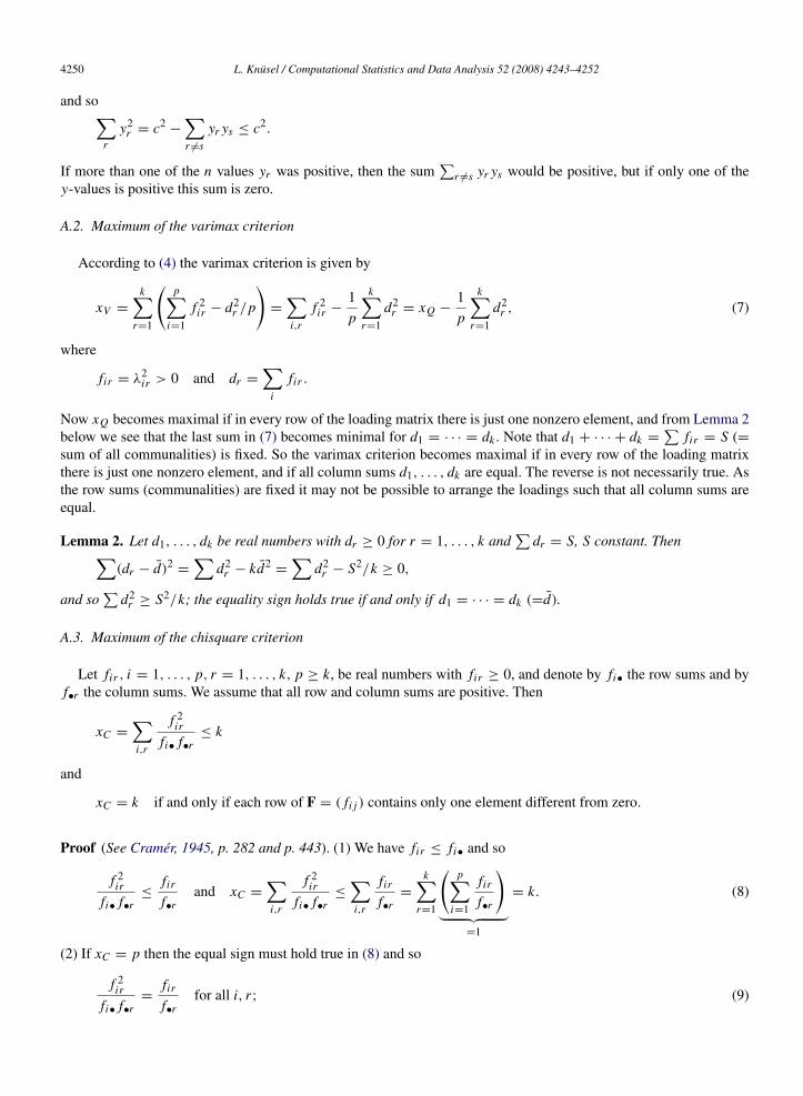
If more than one of the n values yr was positive, then the sum∑

r 6=s yr ys would be positive, but if only one of they-values is positive this sum is zero.

A.2. Maximum of the varimax criterion

According to (4) the varimax criterion is given by

xV =

k∑r=1

(p∑

i=1

f 2ir − d2

r /p

)=

∑i,r

f 2ir −

1p

k∑r=1

d2r = xQ −

1p

k∑r=1

d2r , (7)

where

fir = λ2ir > 0 and dr =

∑i

fir .

Now xQ becomes maximal if in every row of the loading matrix there is just one nonzero element, and from Lemma 2below we see that the last sum in (7) becomes minimal for d1 = · · · = dk . Note that d1 + · · · + dk =

∑fir = S (=

sum of all communalities) is fixed. So the varimax criterion becomes maximal if in every row of the loading matrixthere is just one nonzero element, and if all column sums d1, . . . , dk are equal. The reverse is not necessarily true. Asthe row sums (communalities) are fixed it may not be possible to arrange the loadings such that all column sums areequal.

Lemma 2. Let d1, . . . , dk be real numbers with dr ≥ 0 for r = 1, . . . , k and∑

dr = S, S constant. Then∑(dr − d)2

=

∑d2

r − kd2=

∑d2

r − S2/k ≥ 0,

and so∑

d2r ≥ S2/k; the equality sign holds true if and only if d1 = · · · = dk (=d).

A.3. Maximum of the chisquare criterion

Let fir , i = 1, . . . , p, r = 1, . . . , k, p ≥ k, be real numbers with fir ≥ 0, and denote by fi• the row sums and byf•r the column sums. We assume that all row and column sums are positive. Then

xC =

∑i,r

f 2ir

fi• f•r≤ k

and

xC = k if and only if each row of F = ( fi j ) contains only one element different from zero.

Proof (See Cramer, 1945, p. 282 and p. 443). (1) We have fir ≤ fi• and so

f 2ir

fi• f•r≤

fir

f•rand xC =

∑i,r

f 2ir

fi• f•r≤

∑i,r

fir

f•r=

k∑r=1

(p∑

i=1

fir

f•r

)︸ ︷︷ ︸

=1

= k. (8)

(2) If xC = p then the equal sign must hold true in (8) and so

f 2ir

fi• f•r=

fir

f•rfor all i, r; (9)

L. Knusel / Computational Statistics and Data Analysis 52 (2008) 4243–4252 4251

thus either fir = 0 or fir = fi• which means that each row of F = ( fir ) contains only one element different fromzero.

(3) If each row of F = ( fir ) contains only one element different from zero then we have either fir = 0 or fir = fi•for all i, r and so (9) holds true and thus

xC =

∑i,r

f 2ir

fi• f•r=

∑i,r

fir

f•r= k.

So our proof is complete. Note that we have assumed that all column sums f•r are positive; if one column sum werezero this column would be eliminated in the computation of xC and so the maximum would be reduced from k tok − 1.

A.4. R function to compute the chisquaremax solution of Section 3

References

Browne, M.W., 2001. An overview of analytic rotation in exploratory factor analysis. Multivariate Behavioral Research 36, 111–150.Cramer, H., 1945. Mathematical Methods of Statistics. Princeton University Press.

4252 L. Knusel / Computational Statistics and Data Analysis 52 (2008) 4243–4252

Harman, H.H., 1976. Modern Factor Analysis, third edition, revised. University of Chicago Press, Chicago.Knusel, L., 2008. Factor analysis: Chisquare as rotation criterion. Working paper at the University of Munich. To be obtained from URL:

www.stat.uni-muenchen.de/˜knuesel.Lawley, D.N., Maxwell, A.E., 1971. Factor Analysis as a Statistical Method, second edition. Butterworths London.Maple, 2006. Waterloo Maple Inc. URL: www.maplesoft.com.R Development Core Team, 2006. R: A language and environment for statistical computing. R Foundation for Statistical Computing, Vienna,

Austria. ISBN 3-900051-07-0, URL: www.R-project.org.