Embed Size (px)
Citation preview

Chiral effective field theory withmachine learningBachelor of Science Thesis for the Engineering Physics Program
JOHANNES ASPMAN, EMIL EJBYFELDT,ANTON KOLLMATS, MAXIMILIAN LEYMAN
Department of PhysicsCHALMERS UNIVERSITY OF TECHNOLOGYGothenburg, Sweden 2016

1

bachelor of science thesis for the engineering physics program
Chiral effective field theory with machine learning
Johannes AspmanEmil EjbyfeldtAnton Kollmats
Maximilian Leyman
Department of PhysicsDivision of Subatomic and Plasma Physics
CHALMERS UNIVERSITY OF TECHNOLOGYGothenburg, Sweden 2016

Chiral effective field theory with machine learningJohannes Aspmana, Emil Ejbyfeldtb, Anton Kollmatsc, Maximilian Leymand
Email:[email protected]@[email protected]@student.gu.se
© Johannes Aspman, Emil Ejbyfeldt, Anton Kollmats, Maximilian Leyman, 2016
Bachelor thesis at the Department of Physics, ChalmersBachelor’s thesis TIFX04-16-04
Supervisor: Andreas Ekström, Christian ForssénExaminer: Daniel Persson
Department of PhysicsChalmers University of TechnologySE-412 96 GothenburgSwedenTelephone: +46 31-772 10 00
Cover:Joint probability distribution of the binding energy of the alpha particle and the radius of thedeuteron, see Chapter 5.
Chalmers ReproserviceGothenburg, Sweden 2016

AbstractMachine learning is a method to develop computational algorithms for making predictions basedon a limited set of observations or data. By training on a well selected set of data points it is inprinciple possible to emulate the underlying processes and make reliable predictions.
In this thesis we explore the possibility of replacing computationally expensive solutions of theSchrödinger equation for atomic nuclei with a so-called Gaussian process (GP) that we train on aselected set of exact solutions. A GP represents a continuous distribution of functions defined bya mean and a covariance function. These processes are often used in machine learning since theycan be made to emulate a wide range of data by choosing a suitable covariance function.
This thesis aims to present a pilot study on how to use GPs to emulate the calculation ofnuclear observables at low energies. The governing theory of the strong interaction, quantum chro-modynamics, becomes non-perturbative at such energy-scales. Therefore an effective field theory,called chiral effective field theory (χEFT), is used to describe the nucleon-nucleon interactions.
The training points are selected using different sampling methods and the exact solutions forthese points are calculated using the research code nsopt. After training at these points, GPsare used to mimic the behavior of nsopt for a new set of points called prediction points. In thisway, results are generated for various cross sections for two-nucleon scattering and bound-stateobservables for light nuclei.
We find that it is possible to reach a small relative error (sub-percent) between the simulator,i.e. nsopt, and the emulator, i.e. the GP, using relatively few training points.
Although there seems to be no obvious problem for taking this method further, e.g. emulatingheavier nuclei, we discuss some areas that need more critical attention. For example some observ-ables were difficult to emulate with the current choice of covariance function. Therefore a morethorough study of different covariance functions is needed.
SammandragMaskininlärning är en metod för att utveckla beräkningsalgoritmer som gör prediktioner från enbegränsad mängd observationer eller data. Genom att träna på en mängd väl valda datapunkterär det möjligt att emulera de underliggande processerna och göra pålitliga prediktioner.
I denna rapport undersöker vi möjligheterna att ersätta beräkningstunga lösningar till Schrödin-gerekvationen för atomkärnor med en så kallad gaussisk process (GP) som vi tränar på en valdmängd exakta lösningar. En GP representerar en kontinuerlig distribution av funktioner somdefinieras av ett medelvärde och en kovariansfunktion. Dessa processer används ofta inom mask-ininlärning då de kan emulera en mängd olika typer av data genom att välja en passande kovari-ansfunktion.
Denna rapport syftar till att vara en introduktionsstudie i användandet av GP:s för att emuleraberäkningar av observabler inom kärnfysiken. Den ledande teorin för den starka kraften, kvantkro-modynamik, blir icke-perturbativ vid de låga energier som är relevanta för kärnfysiken, och därföranvänds istället en effektiv fältteori, kallad kiral effektiv fältteori (χEFT), för att beskriva nukleon-nukleon växelverkan.
Träningspunkterna väljs med hjälp av olika metoder och de exakta lösningarna i dessa punkterberäknas med forskningskoden nsopt. Efter att ha tränat på dessa punkter användes GP:s tillatt emulera beteendet hos nsopt för en ny uppsättning punkter som kallas för prediktionspunkter.Resultat tas sedan fram för olika tvärsnitt för tvånukleonspridning samt för bundna tillstånd förlätta atomkärnor.
Vi finner att det är möjligt att nå små relativa fel (sub-procent) mellan simulatorn, dvs nsopt,och emulatorn med relativt få träningspunkter.
Även om det inte finns några uppenbara hinder för att utnyttja denna metod för mer komplexasystem, som tyngre atomkärnor, diskuterar vi vissa områden som behöver mer uppmärksamhet.Exempelvis var vissa observabler svåra att emulera med den använda kovariansfunktionen. En mergenomgående studie av olika kovariansfunktioner skulle därför behövas.

AcknowledgementsWe would like to thank our supervisors Christian Forssén and Andreas Ekström for their supportand guidance during this project. We would also like to express our appreciation to Boris Carlssonfor his support in questions regarding nsopt.
The Authors, Gothenburg, May 2016

Contents
1 Introduction 11.1 Purpose and aims . . . . . . . . . . . . . . . . . . . . . . . . . . . . . . . . . . . . . 11.2 Method and limitations . . . . . . . . . . . . . . . . . . . . . . . . . . . . . . . . . 21.3 Structure of the thesis . . . . . . . . . . . . . . . . . . . . . . . . . . . . . . . . . . 2
2 Gaussian processes for machine learning 32.1 Gaussian process . . . . . . . . . . . . . . . . . . . . . . . . . . . . . . . . . . . . . 32.2 Regression analysis with Gaussian processes . . . . . . . . . . . . . . . . . . . . . . 32.3 Covariance functions . . . . . . . . . . . . . . . . . . . . . . . . . . . . . . . . . . . 52.4 Optimization of the hyperparameters . . . . . . . . . . . . . . . . . . . . . . . . . . 52.5 A basic example . . . . . . . . . . . . . . . . . . . . . . . . . . . . . . . . . . . . . 5
3 Underlying theory of the simulator 73.1 Effective theories . . . . . . . . . . . . . . . . . . . . . . . . . . . . . . . . . . . . . 7
3.1.1 Chiral effective field theory . . . . . . . . . . . . . . . . . . . . . . . . . . . 73.1.2 Low-energy parameters and their statistical errors . . . . . . . . . . . . . . 8
3.2 Scattering theory . . . . . . . . . . . . . . . . . . . . . . . . . . . . . . . . . . . . . 93.3 Bound-states and the many-body problem . . . . . . . . . . . . . . . . . . . . . . . 10
4 Statistical framework for sampling 124.1 Latin hypercube sampling . . . . . . . . . . . . . . . . . . . . . . . . . . . . . . . . 124.2 Sampling the statistical error space of correlated parameters . . . . . . . . . . . . . 13
4.2.1 The covariance of the low-energy constants in NLO . . . . . . . . . . . . . . 134.2.2 Sampling from covariance matrix . . . . . . . . . . . . . . . . . . . . . . . . 13
5 Results 155.1 Calculating cross sections using Gaussian processes . . . . . . . . . . . . . . . . . . 15
5.1.1 The total cross section . . . . . . . . . . . . . . . . . . . . . . . . . . . . . . 155.1.2 Differential cross sections and Azx . . . . . . . . . . . . . . . . . . . . . . . 165.1.3 Propagating statistical errors in LECs . . . . . . . . . . . . . . . . . . . . . 17
5.2 Bound-states . . . . . . . . . . . . . . . . . . . . . . . . . . . . . . . . . . . . . . . 195.2.1 Correlation between binding energy and point-proton radius . . . . . . . . . 195.2.2 Relative errors and time-scales . . . . . . . . . . . . . . . . . . . . . . . . . 20
5.3 Calculation time for the algorithm . . . . . . . . . . . . . . . . . . . . . . . . . . . 21
6 Discussion 226.1 Predicting cross sections . . . . . . . . . . . . . . . . . . . . . . . . . . . . . . . . . 22
6.1.1 Difficulties in predicting some behaviours of the cross sections . . . . . . . . 226.2 Bound-state observables . . . . . . . . . . . . . . . . . . . . . . . . . . . . . . . . . 236.3 Systematic emulator uncertainties . . . . . . . . . . . . . . . . . . . . . . . . . . . 236.4 Hyperparameters . . . . . . . . . . . . . . . . . . . . . . . . . . . . . . . . . . . . . 236.5 Time and memory complexity . . . . . . . . . . . . . . . . . . . . . . . . . . . . . . 23
v

7 Conclusions and recommendations 257.1 Covariance functions . . . . . . . . . . . . . . . . . . . . . . . . . . . . . . . . . . . 257.2 Scikit-learn 0.14.1 . . . . . . . . . . . . . . . . . . . . . . . . . . . . . . . . . . . . . 257.3 Time complexity . . . . . . . . . . . . . . . . . . . . . . . . . . . . . . . . . . . . . 257.4 Outlook . . . . . . . . . . . . . . . . . . . . . . . . . . . . . . . . . . . . . . . . . . 26
Bibliography 27
vi

Chapter 1
Introduction
Modern day physics very often require large amounts of computational power. This is due tothe fact that you often want to solve equations depending on many parameters, resulting in largesystems of equations. Such calculations often become time-consuming despite the computationalcapacity of modern computers.
One way to circumvent this problem is by using a method called machine learning. In themachine learning process a computer is allowed to train on a limited amount of data points andthen use this training to predict the outcomes of similar processes. The goal is to replace theoriginal simulation of the process with an emulator with reduced computational complexity andthereby drastically reduce the time of computation.
Machine learning is a vast scientific field with a wide range of applications. In this thesis, wewill focus on an aspect of machine learning called regression analysis, and more specifically on theGaussian process model of regression analysis. This model uses the mean and covariance betweenthe training points to estimate the targeted function, called the simulator.
Earlier studies have shown that machine learning can be used to increase the effectiveness ofcalculations within fields such as cosmology, many-body physics as well as nuclear physics [1, 2, 3].In this project, we will examine whether it is possible to utilize machine learning to predict crosssections in nucleon-nucleon scattering, as well as propagating the statistical uncertainties in thedescription of the nuclear interaction to bound-state energies of few-nucleon systems.
We will use an effective description of the strong force for nuclear physics, called chiral effectivefield theory (χEFT), to describe the nucleon-nucleon interaction. χEFT uses an expansion ofterms proportional to (Q/Λ)ν to describe the force between the nucleons, where Q and Λ areparameters representing the soft and the hard energy scales of the effective theory. The numberν = 0, 1, 2 . . . determines the size of the term and is called the chiral order. Since the expansioncontains an infinite number of terms a truncation is made whereby the higher order terms areomitted. The most important terms in χEFT have ν = 0 and are labeled the leading order (LO).The next-to-leading order (NLO) have ν = 2, since ν = 1 is forbidden for symmetry reasons, andso on [4].
1.1 Purpose and aimsThis thesis is an introductory study on the effects of using Gaussian processes to emulate observ-ables of nuclear physics. The aim is to give an overview of both the benefits and the costs of thismodel, as well as to present some possible directions for further studies.
The present study is guided by the following three research questions:
• Is it possible to implement an emulator capable of learning from the exact solutions of thenuclear Schrödinger equation and from this make reliable predictions for the nuclear many-body problem?
• For which levels of complexity does this emulator maintain its effectiveness?
• What are the limitations of using machine learning to predict physical systems?
1

1.2 Method and limitationsOur initial studies were mainly directed towards reading literature about practical examples of theuse of machine learning in physics as well as on the underlying theory of Gaussian processes. Thetheory behind χEFT was only given minor attention. Most of the work was carried out in Python,using Scikit-learn 0.14.1, where the code for our emulator was written [5]. To gather training datafor our emulator we used the simulator nsopt. This is a research code for obtaining numericallyexact solutions of the few-nucleon Schrödinger equation.
We focus on calculating observables at NLO in the expansion of χEFT. The machine learningimplemented in the emulator is limited to regression by Gaussian processes, with only the squaredexponential used as covariance function. As for the physics, we will restrain ourselves to trainingour emulator to extrapolate observables associated with bound-states for less than four nucleonsand nucleon-nucleon scattering cross sections, with the ability to propagate errors.
1.3 Structure of the thesisChapters 2 to 4 present the theoretical basis of the thesis. The Gaussian processes which makeup the foundation for this thesis are given a basic description in Chapter 2. Chapter 3 presentsan introduction to effective theories in general and outlines the χEFT and the physical equationsrelevant to our computational models. In Chapter 4 we present the sampling methods used togenerate relevant data points for the Gaussian processes.
Our results for the emulation of scattering and bound-state observables are presented in Chap-ter 5, and these are given a more general discussion in Chapter 6. The thesis is concluded inChapter 7 with a summary and an outlook for further research.
2

Chapter 2
Gaussian processes for machinelearning
In this chapter a short introduction to the theory of Gaussian processes is presented, and a dis-cussion is given on how these are implemented in machine learning. The statistical formulationof regression analysis is presented, along with a discussion regarding the role of the covariancefunction. The chapter is concluded with an example where a Gaussian process is used in regressionanalysis of a simple mathematical function.
2.1 Gaussian processA collection of normally distributed random variables is known as a Gaussian process (GP) [6].There exist several equivalent interpretations of the GP, of which we shall adapt the so calledfunction-space-view.
In the function-space-view, the GP represents a distribution over functions, which is denotedas
f(x) ∼ GP(m(x), k(x,x′)), (2.1)
where the function f is a random variable specified by an argument x. In general, a GP is definedby its mean- and covariance functions, which are denoted as m(x) and k(x,x′), respectively.Thus, the above distribution is effectively a distribution over random functions compliant with thespecified correlations.
In machine learning, the GP is used as a tool for regression analysis by eliminating functionsnot coherent with observed data, which for a GP is known as the training data. The method bywhich non-interesting distributions are removed is probabilistic conditioning [6].
2.2 Regression analysis with Gaussian processesSuppose F is a function of x whose explicit evaluation is computationally cumbersome, makingdirect evaluation on its entire domain highly inefficient. By evaluating the function on a small,but carefully selected, subset of its domain one can try to reduce the computational complexity byemulating F with a GP thus hopefully enabling more efficient, but less accurate, predictions to bemade on its entire domain.
These predictions are made by extrapolating the values assumed by F in the vicinity of a fewsampled points, referred to as training points. There is no general method for choosing the besttraining points, it is an optimization problem of its own [6]. The points for which F is to bepredicted are henceforth referred to as the prediction points, which represent another subset of thedomain of F . The set of x-values specifying the prediction- and training points shall be denoted D,for reference in this chapter.
3

0 2 4 6 8 10
x
−2.0
−1.5
−1.0
−0.5
0.0
0.5
1.0
1.5
2.0
2.5G
P(x
)
(a)
0 2 4 6 8 10
x
−5
0
5
10
15
20
(b)
Figure 2.1: Black lines represent samples drawn from the prior distribution (a) and from the posteriordistribution with 5 training points, marked by × (b) of a Gaussian process with a squared exponentialcovariance function.
As mentioned in the beginning of this chapter, a GP is specified by its mean- and covariancefunctions, m(x) and k(x,x′). One general property that these functions share is that they must bedefined for all values of D. While it is often the case that the mean can be set identically to zero,the choice of covariance function is not as straight forward. As the purpose of the sought GP is toreplicate the behavior of the real function, F , it is necessary to select a covariance function thathas characteristics similar to those of the original function. For this reason, as was the case withthe selection of training points, the procedure of finding a suitable covariance function is heavilydependent on the nature of F (see Section 2.3 for a more elaborate description).
The specified mean- and covariance functions span a distribution of functions (called the priordistribution), as in Equation (2.1) and it is the aim of GP modeling to use the training pointsto extract the set of functions that are most similar to F (called the posterior distribution). Aschematic picture of such a process is shown in Figure 2.1. Every function specified by the GPrepresents a particular joint event of a random variable that corresponds to a point x in D. It isthen a matter of probabilistic conditioning to single out the functions coherent with the trainingpoints. This results in a set of Gaussian distributions for to every x in D [6].
It is convenient to arrange the arguments and the function values of the training points inmatrices, such that
Xt =
x1
x2
...xnt
, Yt =
F (x1)F (x2)
...F (xnt)
, (2.2)
where nt is the number of training points.Similarly, we arrange the points xnt+1,xnt+2, . . .xnt+np for which the function will be predicted
in a matrixXp, where np denotes the number of prediction points. Finally, we introduce the correla-tion matrix, K, defined such that its matrix element Kij = k(xi,xj) where i, j ∈ 1, 2, . . . , nt+np.The correlation matrix becomes
K =
[KXt,Xt KXt,Xp
KXp,Xt KXp,Xp
], (2.3)
where, for instance, KXpXt defines a submatrix of K whose entries corresponds to the pointsdefined by the elements of Xp and Xt. Defining two column vectors, M and Σ2, to contain themean and variances for each x in the posterior distribution in D, it can be shown that [6]
M = KXp,XtK−1Xt,Xt
Yt (2.4)
Σ2 = KXp,Xp −KXp,XtK−1Xt,Xt
KXt,Xp . (2.5)
4

The value of F (x), where x is in Xp, is then estimated by the predicted mean value with itscorresponding variances, extracted from the matrices as
µ(x) =Mx (2.6)
σ2std(x) =
(Σ2
)x. (2.7)
2.3 Covariance functionsWhen modeling a function, F , that can be quite complicated, the objective is to capture its featuresas well as possible, using a minimal amount of training data extracted from the function itself. Themanner in which a GP model accomplishes this is by assuming that adjacent training points exhibitsimilar behavior, and then extrapolate accordingly. In modeling arbitrary functions, this opens upthe freedom to define adjacency by means of a covariance function. As previously established inthis chapter, the adjacency measure is a function of the form k(x,x′).
In theory, any function that is positive semidefinite can be used as a covariance function. Inpractice, the covariance function is best chosen ad hoc to fit a particular problem at hand. Often,this choice is partially done by means of optimizing a set of so-called hyperparameters includedin the function. For some problems, one may wish to combine behaviors of several previouslyknown covariance functions. It can be shown that the addition or multiplication of two covariancefunctions yield another valid covariance function. Similarly, one can produce a new function bytaking the convolution of two covariance functions [6].
One of the most frequently used covariance functions, and also the covariance function usedthroughout this thesis, is the squared exponential, defined as
k(x,x′) = e−|x−x′|2
2l2 . (2.8)
This function has the hyperparameter l, which can be interpreted as a characteristic length scaleof the function F . When modeling smooth functions the squared exponential covariance functionis suitable, since functions drawn from a GP with it are infinitely differentiable.
2.4 Optimization of the hyperparametersThe likelihood is the probability density of the observations given the parameters [6]. The marginallikelihood p(Yt|Xt) is defined as the integral of the likelihood times the prior, where the prior is aprobability distribution answering to our prior knowledge of the parameters. If this knowledge isweak the prior distribution is broad and vice versa.
Using that Yt is normally distributed, with a zero-mean and a covarianceKXtXt , and performingthe integration it can be shown that the log marginal likelihood can be calculated as [6]
log p(Yt|Xt) = −1
2Y ⊤t K
−1XtXt
Yt −1
2log |KXtXt | −
nt2
log 2π. (2.9)
The log marginal likelihood is used to give a measure of how good the model fits the trainingpoints. Since the log marginal gives a value of how good a covariance function is it can be usedto compare different models. But given a covariance function that is dependant on one or morehyperparameters you can formulate a maximization problem of the log marginal likelihood. Solvingthis problem should give you the best hyperparameters for the given training points.
2.5 A basic exampleFor demonstration purposes we will emulate a known one-dimensional target function, which hasbeen chosen arbitrarily as
F (x) = x+ x(sinx− cosx). (2.10)
5

The training data consists of five points, nt = 5, whose x-values are uniformly sampled from theinterval x ∈ [0, 10]. Let, as in (2.2), Xt and Yt denote column vectors whose coordinates arespecified by the values of x and their corresponding samples F and we get
Xt =
13579
, Yt =
1.306.39−1.216.3220.91
. (2.11)
Inferring from these training points, we will predict the values of F corresponding to 100uniformly spaced x-values in the same interval as above, similarly arranged in a column vector Xp.
The x-values are used for calculation of the correlation matrix, specified by the squared expo-nential covariance function of Equation (2.8). For the one-dimensional case, with l = 0.5 to helpillustrate how the hyperparameters affects the prediction, the covariance function is
k(x, x′) = e−2(x−x′)2 . (2.12)
Using the covariance function the correlation matrix of the training points is calculated
KXt,Xt =
1 1.06e − 1 1.26e−4 1.68e−9 2.51e−16
1.06e−1 1 1.06e−1 1.26e−4 1.68e−91.26e−4 1.06e−1 1 1.06e−1 1.26e−41.68e−9 1.26e−4 1.06e−1 1 1.06e−12.51e−16 1.67e−9 1.26e−4 1.06e−1 1
. (2.13)
The hyperparameter l is now optimized by maximizing the log marginal likelihood in Equa-tion (2.9). A maximum is found for l = 1.75, which will be considered the optimal value of l.
Now the full correlation matrix is calculated using the optimal l. The matrix is then decomposedinto submatrices according to (2.3), and the mean and variances for the posterior distribution arederived from (2.4) and (2.5), finally µ(x) and σ2
std(x) are calculated according to (2.6) and (2.7).The standard deviation function σstd(x) has been obtained by taking the positive square root of thevariance function. Figure 2.2 illustrates the prediction for both the initial value of l = 0.5 and theoptimal l = 1.75. The dashed green curve is µ(x), the blue curve is the true target function, F (x),and the shaded area indicates the 2σstd (95%) confidence interval as deduced from the standarddeviation.
0 2 4 6 8 10−10
−5
0
5
10
15
20
25
30
F(x
)
l = 0.50 (a)
F (x) = x+ x(sin x− cos x)
Prediction
95% confidence interval
Training points
0 2 4 6 8 10−10
−5
0
5
10
15
20
25
30
l = 1.75 (b)
Figure 2.2: Example of a Gaussian process used in predicting the function (2.10). Panel (a) shows theprediction with a guessed value of the hyperparameter l = 0.5 and panel (b) shows the prediction for theoptimal value of l = 1.75.
6

Chapter 3
Underlying theory of the simulator
This chapter serves to give an introduction to the physical theories that make up the backboneof this thesis. A brief introduction to effective theories is given and the usefulness of χEFT isestablished. Next, its connection to scattering theory is made. Finally, an introduction to boundstates is provided.
3.1 Effective theoriesIt is widely known that the physical phenomena present at the various scales of the universe appearquite distinct from each other. While, in principle, a theory of everything would be sufficient tomake predictions on any scale, in practice it is often necessary to isolate a set of phenomena andstudy them without considering the effects of irrelevant physics. By diverting attention only tothe relevant degrees of freedom of a physical system, calculations can often be made significantlysimpler, increasing the ability to make predictions. The practice of isolating certain parts ofphysics, relevant only at certain scales, has resulted in so-called effective theories, as shall befurther illustrated below.
The principle of an effective theory can be illustrated by the familiar correspondence of relativistic-and Newtonian mechanics. In inertial frames moving with constant velocities relative to one an-other the relationship between momentum and velocity of an object is a non-linear one. If oneassumes that the object is moving slowly in comparison to the speed of light, one may expandits momentum in terms of a power series with rapidly vanishing terms. For many practical ap-plications, this assumption is plausible and one may simply truncate the series, for reasons ofcomputational simplicity, and yet retain a valid description of the physics observed at this par-ticular velocity scale. By discarding all but the leading-order term (LO), one obtains the classicexpression for momentum, for which only the first power of velocity is a relevant degree of freedom.Naturally, this introduces a systematic error of the model. However, while a more accurate descrip-tion of the physics is obtained by the inclusion of higher order terms (referred to as expansions ofnext-to-leading-order (NLO), next-to-next-to-leading-order (NNLO), and so on) they are generallynot needed when dealing with classical mechanics [7].
Similarly, one may obtain a relatively simple description of low-energy nuclear forces by meansof a series expansion.
3.1.1 Chiral effective field theoryStrong nuclear forces are described by the theory of quantum chromodynamics (QCD). By meansof a series expansion, low-energy nuclear forces can be given a relatively simple description in termsof an expansion parameter, Q/Λ. The quantities Q and Λ are energies whose magnitudes are ofthe same order as the rest energies of the pion and rho meson, respectively. Thus, Λ defines theenergy scale for which the expansion is valid. This limiting case of QCD is called chiral effectivefield theory, χEFT, and is the physical theory underlying this thesis [4, 8].
In the same manner as with the case of classical- and relativistic mechanics, one obtains aninfinite sum of terms proportional to (Q/Λ)ν , where ν is referred to as the chiral order of the term.
7

Figure 3.1: Schematic figure showing Feynman diagrams representing nucleon-nucleon interactions. Thehorizontal orientation classify the diagrams by the number of nucleons involved, while the vertical directionspecify the order of the term. Solid lines represent nucleons and dashed lines pions. Circles, diamondsand squares represent the chiral order of the interaction. The order ν = 1 does not contain any newdiagrams because of parity- and time-symmetries. At the order ν = 3 (NNLO), diagrams for three-nucleoninteractions (NNN) are also present.
Each term can be interpreted to represent a finite set of interaction diagrams, known as Feynmandiagrams. Shown in Figure 3.1 are Feynman diagrams representing nucleon-nucleon interactions.The diagrams are arranged schematically with the vertical orientation representing the order ofthe term associated with the diagrams, while the horizontal orientation classify the diagrams bythe number of nucleons involved. Two-nucleon interactions are denoted as NN and three-nucleoninteractions by NNN. As for the diagrams themselves, the lines represent particles propagatingthrough space-time, with solid lines for nucleons and dashed lines for pions. Circles, diamonds andsquares represent the chiral order of the interactions and their corresponding coupling constants,a measure of the relative strengths among the interactions [9, 10].
As seen in Figure 3.1, several diagrams correspond to a single term in the expansion, whereeach term itself is given by the sum of the contributions from short-range interactions as well asthe exchange of a number of pions. For reasons of parity- and time-symmetry terms with powersν = 1 vanish, resulting in the inclusion of terms with ν ≤ 2 in the NLO-expansion. As alsoindicated in Figure 3.1, diagrams corresponding to three-nucleon interactions are not present untilan expansion up until NNLO, which is to be expected as three-nucleon interactions are significantlyweaker than that of two-nucleons. The effective field theory is obtained by discarding the weak,higher order terms, completely analogous to the truncation of the relativistic momentum expansionin the example above.
3.1.2 Low-energy parameters and their statistical errorsEffective field theories are governed by certain parameters, referred to as low-energy constants(LECs) in the case of χEFT for nuclear physics. The dimension of the parameter space is dictatedby the chiral order of the expansion. For instance at LO and NLO there are 2 and 9 LECs respec-tively. The parameters are determined by means of fitting model predictions to experimental data.Effectively, this amounts to determination of the coupling coefficients mentioned in Section 3.1.1.In our case, the data stem from experiments in nucleon-nucleon scattering, where the measuredobservable is scattering cross sections (see Section 3.2 for details) [9].
Since the LECs are determined from experimental data, which always exhibit a certain uncer-tainty, the LECs themselves inherit some flexibility in their determined values. This uncertaintyis referred to as the statistical error of the model.
The LECs also exhibit a certain dependence on each other due to the fact that they describethe same physics. So if the value of one is changed the others will also be changed. This results inthe need to use their covariance matrix when propagating the statistical errors (for further details
8
see Section 4.2).
3.2 Scattering theoryMost of this thesis revolves around the computation of one specific type of observable: nuclearcross sections, denoted σ. It is a measure of how many of the incident particles of a beam arescattered from a target particle, and experimental measurements of the cross section have beenused to determine the size and shape of the atomic nucleus [11]. For convenience we will neglectthe spin-dependence of the nuclear force in this section.
If you know the flux of incoming particles and measure the amount of outgoing scatteredparticles you can calculate the probability scattering. That probability corresponds to the crosssection, σ. The rate at which a reaction takes place, Wr, is proportional to the flux of incomingparticles, J , and the number of particles in the target, N , hit by the beam.
Wr = JNσ (3.1)
Usually what is measured is just a differential reaction rate, dWr, since the detectors commonlyused do not measure all the scattered particles,
dWr = JNdσ
dΩdΩ (3.2)
where dσdΩ is the differential cross section and dΩ = sin θ dθ dϕ is the differential solid angle sub-
tended by the detector as shown in 3.2. In order to obtain the total cross section you have tointegrate the differential cross section over all angles [11],
σtot =
∫ 2π
0
dϕ
∫ π
0
sin θ dθdσ
dΩ. (3.3)
If one would use a beam of polarized particles and/or a polarized target particle the situationbecomes more complex. The polarization is given as the expectation value of the spins of allparticles in the target or beam and can be changed by rotating the spins of the particles using amagnet.
The cross section of this scattering will show azimuthal asymmetry from which the transversecomponent of the polarization can be determined. By rotating the spin it is also possible todetermine the longitudinal part of the polarization [12]. Due to the combinations of polarized,unpolarized beams and targets there are many different types of cross sections, for some examplesof this see Figure 3.3. In this thesis we will focus on calculating only three different cross sections,selected because of their varying degrees of complexity. These are the total cross section, σtot,a differential cross section where both target and beam are unpolarized, dσ
dΩ , and a cross sectionwhere the beam and target are polarized in the x-z plane, Azx, as shown in Figure 3.3 [12].
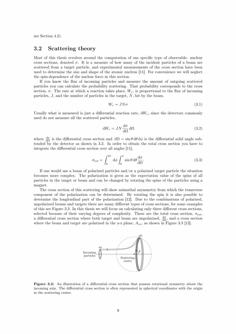
Figure 3.2: An illustration of a differential cross section that possess rotational symmetry about theincoming axis. The differential cross section is often represented in spherical coordinates with the originin the scattering center.
9

Figure 3.3: Scattering experiments with different combinations of polarizations for beam and target.Polarization is represented with an arrow and ⊙ is an arrow out of the page.
The total cross section depends on the energy of the incoming beam, while being independentof the angle, θ, between the beam and target, while the differential cross sections, dσ
dΩ and Azx,are dependent on both energy and θ. Figure 3.4 shows these cross sections calculated with nsopt
in NLO. Azx assumes negative values in Figure 3.4 for some values of the energy and θ. This isbecause it is normalized against the unpolarized differential cross section.
0 50 100 150 200 250 300
Lab energy [MeV]
101
102
103
104
Tota
lcr
oss
sect
ion
[mb]
0 50 100 150 200 250 300
Lab energy [MeV]
0
20
40
60
80
100
120
140
160
180
θ[d
egre
es]
0
2
4
6
8
10
12
14
16
18
20
dσ
dΩ
[mb]
0 50 100 150 200 250 300
Lab energy [MeV]
0
20
40
60
80
100
120
140
160
180
θ[d
egre
es]
−0.45
−0.30
−0.15
0.00
0.15
0.30
0.45
0.60
Azx
Figure 3.4: The three different cross sections studied in this thesis, calculated with nsopt for the LECvalues given in Table 4.1 for NLO. The reasons for the chosen intervals of θ and energy are that for anglesgreater than 180 you only receive a mirroring of the cross section, and the 300MeV limit is set becauseof the limits of χEFT.
3.3 Bound-states and the many-body problemOne important and often occurring task in nuclear physics is the calculation of properties forbound-states in the nucleus. For nuclei consisting of more than one nucleon this requires solvingthe many-body Schrödinger equation. One model often used for computing few-nucleon states isknown as NCSM, or the no-core-shell-model. Here the problem is to find the eigenvalues given bythe many-body Hamiltonian [13]
H =A∑
j=1
tj +A∑
j<k=1
v2,jk +A∑
j<k<l=1
v3,jkl + . . . (3.4)
where tj represents the kinetic energies of the different nucleons and v2,jk and v3,jkl represents thetwo- and three-nucleon interactions respectively.
If |ψ⟩ is an eigenstate of this Hamiltonian
H |ψ⟩ = E |ψ⟩ (3.5)
you can express |ψ⟩ in an orthonormal complete harmonic oscillator basis |ϕi⟩ as
|ψ⟩ =∑i
ci |ϕi⟩ . (3.6)
which turns the Schrödinger equation into
HN∑i
ci |ϕi⟩ = EN∑i
ci |ϕi⟩ . (3.7)
10

Since the sum is infinite you need to truncate it at some finite N .If we now multiply the equation by ⟨ϕj | we get
N∑i
ci ⟨ϕj |H |ϕi⟩ = EN∑i
ci⟨ϕj |ϕi⟩, (3.8)
but since the basis is orthonormal the right-hand side becomes Ecj and on the left-hand sideyou have ⟨ϕj |H |ϕi⟩ which corresponds to the matrix element Hji of the Hamiltonian, and themany-body Schrödinger equation results in an eigenvalue problem
Hjici = Ecj (3.9)
which is solved by diagonalizing the matrix of the Hamiltonian. The lowest eigenvalue Ei givesthe ground state energy of the system represented by the Hamiltonian. The eigenvector c providesthe amplitudes of the corresponding wave function |ψ⟩ in the basis |ϕi⟩. For a more thoroughdescription of this see [13].
One of the quantities that we will be working with is the theoretically calculated point-protonradius which is related to electric charge radius measured in experiments. This can be calculatedusing the eigenvectors obtained in the diagonalization of the Hamiltonian [10].
11

Chapter 4
Statistical framework for sampling
An important aspect to consider when creating an efficient machine learning emulator is how toselect your training data. This chapter serves to present the different sampling techniques usedin this thesis. The latin hypercube sampling is introduced as an effective way of sampling, and adiscussion on how to sample from a correlated set of parameters concludes the chapter.
4.1 Latin hypercube samplingThe latin hypercube sampling (LHS) was introduced by Mackay et al. in 1979 [14], and has beenused extensively in fields where an efficient sampling method is needed [15, 16]. Earlier studieshave shown that LHS is preferable in Gaussian process modeling [1, 16].
LHS is generated by dividing every axis of the sample space into a number of intervals, N , withequal marginal probability, 1/N . For every axis and every interval, one, and only one, coordinateis picked randomly, and together these coordinates define the N sample points [14].
Figure 4.1 demonstrates LHS used on a two dimensional sample space and five sample points,where the dots are the different sample points and the grid outlines the five sampling intervals forevery axis.
0.0 0.2 0.4 0.6 0.8 1.00.0
0.2
0.4
0.6
0.8
1.0
Figure 4.1: Latin hypercube sampling (LHS) performed for two dimensions with five sample points. Intwo-dimensional LHS, the points are distributed in a manner that ensures the presence of only one pointper row and column.
There are several different categories of LHS, stemming from different constraints put on howthe samples are selected inside the intervals. For instance they can be chosen randomly insidethe given intervals, or with the criteria that they should be picked so to maximize the minimumdistance between sampling points, LHSmm [15].
12

We will use a package for Python called pyDOE that generates a latin hypercube sample for anynumber of dimensions and sample points [17]. This package also allows you to put different criteriaon how to sample the points inside the given intervals, where we will examine both the criteria ofmaximizing the minimum distance between points as well as to select them randomly.
4.2 Sampling the statistical error space of correlated param-eters
The parameters, i.e. the so-called LECs, we use have been obtained from separate fits to ex-perimental data, and as such they exhibit a certain statistical error. The parameters with theirstatistical errors, taken from [9], are shown in Table 4.1.
Table 4.1: The LECs from NLO with their 1σ uncertainty (given in the parenthesis) taken from [9].
LECs from NLO
C(np)1S0
−0.150623(79)
C(pp)1S0
−0.14891(11)
C(nn)1S0
−0.14991(27)
C1S0+1.6935(83)
C3S1−0.1843(16)
C3S1−0.218(14)
CE1 +0.263(16)C3P0
+1.2998(85)C1P1
+1.025(59)C3P1
−0.336(10)C3P2
−0.2029(15)
4.2.1 The covariance of the low-energy constants in NLOThe LECs of χEFT hold a dependency on each other which has to be accounted for when samplingover their error space [9]. The correlation matrix of the LECs in NLO is presented in Figure 4.2.This is a symmetric matrix with element
Cij = corr(ci, cj) =cov(ci, cj)σciσcj
(4.1)
where ci are the different LECs and cov(ci, cj) is the covariance between LECs ci and cj , a resultof the statistical fit of the LECs in [9]. A value of Cij = −1 means that parameters ci, cj are fullyanti-correlated, and a value of +1 means that they are fully correlated.
4.2.2 Sampling from covariance matrixSince the parameters have a certain dependence on each other, a correlation matrix must be usedto form orthogonal vectors with corresponding error estimates and a normally distributed sampleis taken over the variance of these vectors. To capture the properties of this distribution, samplingwill be done from a multivariate Gaussian distribution [18].
More explicitly, this is done via a linear transformation of the parameters with the eigenvectorsof the correlation matrix as the coefficients of the transformation matrix. If αi is our transformedparameter with index i and αi the original, we get
αi = vi,1α1 + vi,2α2 + · · ·+ vi,11α11 (4.2)
with the different v’s being the different eigenvectors of the correlation matrix. For the wholevector of parameters we get
13

C(np)
1S0
C(pp)
1S0
C1S0
C3S1
C3S1
CE
1
C3P0
C1P1
C3P1
C3P2
C(nn)
1S0
C(np)1S0
C(pp)1S0
C1S0
C3S1
C3S1
CE1
C3P0
C1P1
C3P1
C3P2
C(nn)1S0
−1
0
1
Figure 4.2: Correlation matrix of LECs in NLO constructed using data from [9]. The eccentricity of theellipses correspond to the value of the correlation while the slope of the major axis determines whether theLECs are correlated or anti-correlated. The squares describes the correlation according to the colorbar.−1 means fully anti-correlated and +1 means fully correlated.
α = V α =⇒ α = V −1α (4.3)
where V is the matrix of eigenvectors received from the diagonalization of the covariance matrix.The eigenvector of the correlation matrix corresponding to the largest eigenvalue represents the
direction in which the sample varies the most, and so on. The corresponding eigenvalues representsthe magnitudes of these variances [19]. By multiplying the eigenvectors with the LECs, the samplespace is rotated and it is then possible to sample independent vectors along the rotated interval.Finally, the matrix of eigenvectors is inverted and multiplied with the rotated parameters as inEquation (4.3).
It is still important to recognize that the uncertainties given in Table 4.1 are the 1σ deviationwhen assuming that the parameters are normally distributed. In this thesis, in order to accountfor this, we do the LHS over the previously mentioned multivariate Gaussian distribution.
14

Chapter 5
Results
This chapter presents the results of using Gaussian processes to emulate certain observables innuclear physics. We first present the results from predicting different cross sections. After that wepresent some introductory results from predicting bound-states of nuclear physics. The chapterends with results concerning the time efficiency of the Gaussian processes.
5.1 Calculating cross sections using Gaussian processesThe cross sections that we study in this thesis are from neutron-proton scattering. The resultsin Sections 5.1.1 and 5.1.2 are based on a set of LECs according to the mean values given inTable 4.1. In Section 5.1.3 however, we perform and present the results from an error propagationof the statistical uncertainties given in the same table.
The emulator was trained using differently sized training data sets and the predicted valueswere compared to exact data computed with nsopt.
Figure 5.1 shows the relative error of the emulator, compared to the data from nsopt, fromthe prediction of Azx with 10, 100 and 1000 training points. It shows that the relative errorsare symmetrically distributed around zero, and we use the standard deviation as a measure ofthe quality of the emulator. Similar results were found for the distribution of the errors of allemulations done in this thesis.
−0.6 −0.3 0.0 0.3 0.6
Relative error
0
2000
4000
6000
8000
10000
12000
Counts
10 tr. points
−0.03 0.00 0.03
Relative error
0
5000
10000
15000
20000
100 tr. points
−0.0001 0.0000 0.0001
Relative error
0
5000
10000
15000
20000
25000
30000
35000
1000 tr. points
Figure 5.1: The distribution of the relative error of the emulator against data from the simulator, nsopt,for Azx predictions using 10, 100 and 1000 randomly sampled training points.
5.1.1 The total cross sectionFor a given set of fixed LECs, the total cross section depends only on the energy of the incomingbeam.
15

The blue line in Figure 5.2(a) shows the standard deviation of the relative error between ouremulator and nsopt for different sizes of the training data set. We used 10, 100, 500 and 1000training points selected with equal spacing on the energy interval, and the predictions were cross-validated against a set of 2000 calculations with nsopt.
One problem with predicting the total cross section was its great variance between high andlow energies. In order to flatten out this variance, and then see if the precision of the predictionscould be increased, we also trained the emulator using the logarithm of the total cross section.This corresponds to the green dashed line in Figure 5.2(a).
To further illustrate the difference between training with the logarithm of the total cross section,Figure 5.2(b) shows the different results for predicting the total cross section. The blue linecorresponds to using the regular data when training and the green dashed line corresponds totraining on the logarithm of the training points.
200 400 600 800 1000
Number of training points
10−5
10−4
10−3
10−2
10−1
100
101
Std
of
rela
tive
erro
r
(a)
Emulator
Emulator(log)
0 50 100 150 200 250 300
Lab energy [MeV]
101
102
103
104
Tota
lcr
oss
sect
ion
[mb]
(b)
Emulator
Emulator(log)
Simulator (nsopt)
Training points
Figure 5.2: (a) The standard deviation, std, of the relative error when the total cross section was predictedfor various amounts of training points, both with the logarithm of the total cross section and the regularvalues of the total cross section. (b) the total cross section trained with regular data and logarithm takenbefore training for 30 training points.
5.1.2 Differential cross sections and Azx
With fixed LECs, both the unpolarized differential cross section and the polarized Azx depend onlyon the energy of the incoming beam and the scattering angle, θ. Because of the inefficiency of theequal-spacing sampling method in sampling functions of several variables, the training points forthe differential cross section and Azx were sampled using both random sampling and the LHSmmmethod. Both methods were used to obtain training sets with 10, 100, 500 and 1000 points.
The sampling was performed 20 times for every size of the training set. In Figure 5.3 we showthe mean standard deviation of these sets for different number of training points. The width ofthe bands represents the 1σ interval of the standard deviations of the twenty different groups ofsampling points.
Before training the emulator to predict the differential cross section, the logarithm of thetraining data was taken to even out the steepness of the curve for low-energies, as in the abovecase of the total cross section.
16

200 400 600 800 1000
Number of training points
10−4
10−3
10−2
10−1
100
Azx
200 400 600 800 1000
Number of training points
10−3
10−2
10−1
100Std
of
rela
tive
erro
r
dσdΩ
Mean std, random
Mean std, LHS
Figure 5.3: The mean of the standard deviation of the relative error when predicting for differently sizedtraining sets from random sampling and LHSmm for the differential cross section and Azx.
5.1.3 Propagating statistical errors in LECsAt NLO we have a set of 11 LECs. Two of them are only relevant for proton-proton and neutron-neutron interactions. Since we only study the neutron-proton interaction in this thesis, we willonly have to consider a set of 9 LECs, selected from the distribution according to Section 4.2.2.
As a primary implementation, we explored the error propagation abilities of the emulator byvarying the LECs for the total cross section at a single energy, namely Tlab = 19.665MeV. Figure5.4 shows the total cross section values predicted by nsopt (the emulator) on the left (right) handside. The nsopt values have been generated for 100,000 parameter samples. Predictions werethen made with the emulator for the same sets of parameters based on 50 training points. In bothgraphs, a normal distribution specified by the mean value of the total cross section and its standarddeviation is shown in red. The standard deviation of the values predicted by the emulator differson the third decimal from that of nsopt, i.e. a relative uncertainty of order 10−5.
492.0 492.2 492.4 492.6 492.8 493.0 493.2
Total cross section [mb]
0
500
1000
1500
2000
2500
3000
3500
4000
Counts
µ = 492.51σstd = 0.125
492.0 492.2 492.4 492.6 492.8 493.0 493.2
Total cross section [mb]
0
500
1000
1500
2000
2500
3000
3500
µ = 492.52σstd = 0.121
Figure 5.4: The left panel shows the distribution of values calculated for 100,000 parameter samples bynsopt. The right panel instead shows the predictions of the emulator for the same sets of parameters aftertraining on 50 sets. The red curve is the same in both panels and it shows a normal distribution specifiedby the mean and standard deviation of the nsopt distribution.
Additionally, the emulator was used to perform error propagation throughout the entire energyrange. Treating the energy as another parameter, 10 parameters had to be varied simultaneously(9 LECs, 1 energy). The energies were uniformly sampled from the interval 0.5 to 290 MeV. TheLECs were randomly sampled from a normal distribution specified by the mean and standarddeviation of Table 4.1 and covariances as explained in Section 4.2.2.
17

Figure 5.5 show energy on the horizontal axis and the total cross section on the vertical axisfor two different configurations of 100 and 1000 training points respectively. In both cases, theemulator was trained on the logarithm of the total cross section values from nsopt, in the samemanner as in Section 5.1.1. In total, 20 curves were generated from non-identical, but equallysized, training sets for each of the two size configurations. The total cross section values were thenpredicted by the emulator for 1000 points with the LECs held constant, as opposed to the training,throughout the entire energy range.
The precision of the emulator was tested against nsopt. Figure 5.6 shows the mean standarddeviation of the error of the emulator relative to nsopt for various sizes of the training set. Thepredictions were made by the emulator for energies in the 0-290 MeV interval. For every energy,a distinct set of randomly sampled LECs were used. The predictions were made using constantLECs, i.e one set of LECs were used throughout the entire spectrum of energy. Predictions weremade 20 times for training sets of varying sizes (10, 100 and 1000 points).
0 50 100 150 200 250 300
Lab energy [MeV]
101
102
103
104
Tota
lcr
oss
sect
ion
[mb]
0 50 100 150 200 250 300
Lab energy [MeV]
101
102
103
104
Figure 5.5: 20 total cross section curves as predicted by the emulator for energies in the 0-290 MeVinterval. For every energy, a distinct set of randomly sampled LECs were used. On the left (right) atraining set with a total number of 100 (1000) points were used. The subsequent predictions were madeusing non-varying LECs, i.e one set of LECs were used throughout the entire energy range. As can be seenin the left panel, two significant outliers indicate the low precision of the predictions.
0 200 400 600 800 1000
Number of training points
10−2
10−1
100
101
Std
of
rela
tive
erro
r
Figure 5.6: The solid line shows the standard deviation of the relative error when the total cross sectionwas predicted for various amounts of training points. The relative error has been computed as the meanvalue of 20 different sets of parameters for three different set sizes (10, 100 and 1000). Each set of parametersconsists of a number of energies evenly distributed in the interval 0-290MeV, with each energy associatedwith a set of randomly sampled LECs. The predictions that were compared to nsopt were made usingconstant LECs throughout the entire energy range.
18

5.2 Bound-statesSo far we have only looked at scattering observables. However the emulator was also used topredict bound-state observables for systems with up to four nucleons.
To measure the emulator’s efficiency we performed an error propagation for different LEC valuessimilar to the one performed for the cross sections. Training points were sampled from a randommultivariate Gaussian distribution of LECs using the previously mentioned covariance matrix.
The simulator, nsopt, calculates a set of 9 bound-state observables for each set of LECs andcorrelation between these observables has been documented [9].
5.2.1 Correlation between binding energy and point-proton radiusAt N2LO the correlation between the binding energy of the alpha particle E(4He) and the point-proton radius of the deuteron Rpt−p(2H) had previously been plotted as a joint probability distri-bution [9]. That, however, was never done for bound-state observables at the NLO-level which isthe focus of this thesis. Plotting the joint probability distribution of the above named observablesfor this level was therefore the first task in this area. Also the contour lines corresponding to the1σ and 2σ intervals were to be generated in order to better visualize the limits of the distribution.
12,000 sets of LECs were sampled and observables were calculated for each set with nsopt. Thisis the distribution shown in Figure 5.7. The contour lines corresponding to 1σ and 2σ confidenceintervals were then generated and are used as a reference (solid black line) in both Figure 5.7 andFigure 5.8 to show the accuracy of the emulator.
Earlier predictions made for respective observable at NLO had set the limits at 1.970 and1.972 fm for the point-proton radius and −27.3 and −27.6MeV for the binding energy using sta-tistica l analysis[9]. As seen in Figure 5.7 most of the points calculated by nsopt stay within theseintervals.
To test the accuracy of the emulator, two training sets consisting of 50 and 100 training pointswere used to predict the observables of all 12,000 points. The contour lines of these predicteddistributions were also generated, also shown in Figure 5.7.
The dotted blue (dashed red) lines correspond to the 1σ and 2σ intervals of the distributionpredicted by utilizing 50 (100) training points. At 100 training points, the relative error betweenthe predicted data and nsopt are on the order of 10−6 for both observables. A remarkably smallnumber with so few training points.
Figure 5.8 was made in order to get a picture of what the joint probability distribution wouldlook like for a larger number of points. The emulator was provided a set of 100 training points andwas then set to predict the observables for 100,000 new sets of LECs. Contour lines correspondingto 1σ and 2σ were generated to show the confidence intervals for the predicted points, and theseare shown together with the confidence intervals of the 12,000 points from nsopt.
These contours coincide to a great degree and the distribution in Figure 5.8 is very similar tothe one in Figure 5.7. This shows that a valid distribution is obtained even when predicting fornew LEC values. Since so many points are plotted one can assume that the distribution shown inFigure 5.8 is representative of what the real distribution would look like.
19

−28.0 −27.8 −27.6 −27.4 −27.2 −27.0
E(4He) [MeV]
1.966
1.967
1.968
1.969
1.970
1.971
1.972
1.973
1.974
Rpt−p(2
H)
[fm
]
1σ2σ
Figure 5.7: Joint probability distribution of the radius of the deuteron, Rpt−p(2H), and the binding energyof the alpha particle, E(4He) at NLO. The black line is from 12,000 calculations with nsopt, dotted bluelines are from a prediction of 12,000 points using 50 training points and the dashed red line correspondsto a prediction of 12,000 points using 100 training points.
−28.0 −27.8 −27.6 −27.4 −27.2 −27.0
E(4He) [MeV]
1.966
1.967
1.968
1.969
1.970
1.971
1.972
1.973
1.974
Rpt−p(2
H)
[fm
]
1σ2σ
Figure 5.8: Joint probability distribution of the radius of the deuteron, Rpt−p(2H), and the binding energyof the alpha particle, E(4He) for NLO. The black line is from 12,000 calculations with nsopt, dashed redlines are from 100,000 points predicted using 100 training points.
5.2.2 Relative errors and time-scalesIn this section we will give a more rigorous account of how the errors generated by the emulatorwere reduced and show how the processor time scales with the number of training points used.
For a given amount of training points, the procedure of training and predicting was repeated50 times with different training sets. The relative error was taken between the simulator, nsopt,and the emulator for every iteration. The processor time for initialization and predicting were alsomeasured respectively.
The mean of the values generated by the iterations was taken for each number of training pointsin order to eliminate statistical fluctuations.
In Table 5.1 the relative errors as well as the time it took to train and predict for a set numberof training points for the point-proton radius are given. Since the errors and the times were verysimilar for both observables we show only the results for the radius.
It takes approximately 46 seconds for nsopt to calculate one set of observables from a setof LECs on a computer with a quad core CPU clocked at 3.4GHz. Thus, it took 153 hours tocalculate the 12 000 points used as a reference in Figure 5.7 and Figure 5.8. In order to reduce timethe training sets were calculated on separate computers in groups of 1000. If one were to use theemulator instead, time could be drastically reduced as seen in Table 5.1. 40 or 80 minutes would
20

be needed to calculate the number of training points necessary to get an accurate distribution.After that, only seconds would be needed to generate a distribution of 12,000 points.
The relative speedup, defined as the quotient between execution times for nsopt and for theemulator with the same number of prediction points, is also given in Table 5.1. For 50 (100)training points and 12,000 prediction points a remarkable speedup of 240 (120) is obtained whileretaining a relative error on the order of 10−5 (10−6). When we go from 100 to 500 training pointsthe relative speedup is reduced by 80% while the relative error decreases by 89%. However formost tasks a relative error of 10−6 would probably be acceptable.
Table 5.1: Overview of the calculation time and relative error for different number of training points.Training data generation is the approximate time it takes to calculate the training points with nsopt,initialization is the time it takes to prepare the emulator, prediction is the time it takes to calculate 12,000points with the emulator. The relative speedup, compared with the time it would take to calculate 12,000simulations, is shown in the last column.
Number oftraining points
Relativeerror
Training datageneration time [s]
Initializationtime [s]
Predictiontime [s]
Relativespeedup
50 4.82e-5 2300 0.15 0.52 240100 3.86e-6 4600 0.28 0.68 120500 4.32e-7 23,000 4.27 1.14 241000 2.32e-7 46,000 15.20 1.68 12
5.3 Calculation time for the algorithmThe time analysis of the algorithm was divided into three different steps, (a) optimization of thehyperparameters, (b) decomposition of the covariance matrix and (c) predicting new data points.Figure 5.9 shows the calculation time as a function of both the number of training points anddimension of the training space. It can be seen that the prediction step depends linearly on thenumber of training points, while optimization and decomposition exhibit at least a polynomialdependency. It was also shown that the calculation time for the prediction was linearly dependanton the number of prediction points.
0 200 400 600 800 1000
Number of training points
0
1
2
3
4
5
Calculationtime[s]
(a)
1 pars
5 pars
9 pars
0 200 400 600 800 1000
Number of training points
0.0
0.2
0.4
0.6
(b)
0 200 400 600 800 1000
Number of training points
0.0
0.5
1.0
1.5
2.0
(c)
Figure 5.9: The calculation time for differently dimensioned training sets and for three different stepsof the algorithm, (a) optimization, (b) decomposition of the covariance matrix and (c) prediction. (a) thecalculation time for one run of the optimization with a random starting position. (b) the calculation timefor decomposition of the matrices needed in the prediction. (c) calculation time for predicting the valuefor 10,000 points.
21

Chapter 6
Discussion
This chapter includes a discussion and an interpretation of the results from the previous chapter ina broader sense, including the difficulties and uncertainties found in the method. First, a discussionis presented on the prediction of different cross sections and the difficulties therein. The subjectof emulating bound-states is then examined. The chapter ends with a more general discussion onthe benefits and drawbacks of the method.
6.1 Predicting cross sectionsIn predicting the different cross sections we found that the emulator can be quite successful evenwith relatively small amounts of training points. For the total cross section and Azx we get to thesub-percent level of errors for just above 100 training points, see Figures 5.2 and 5.3, while thedifferential cross section reaches a few-percent level around the same amount of training points,Figure 5.3.
6.1.1 Difficulties in predicting some behaviours of the cross sectionsA problem we found with the chosen method was in predicting functions that have a large variancein their values, like the total- and differential cross sections for low versus high energies. This isprobably due to the fact that the covariance function wants to correlate the low-energy points withthe high-energy points where the function takes an almost constant value, much lower than for thelow-energies. Because of this it overfits the data in the transition between slopes, see blue curvein Figure 5.2(b).
One way to circumvent this overfitting is by doing a transformation of the training data todecrease its variance [20]. The green dashed curve in Figure 5.2 shows the improvement in thepredictions when the logarithm of the function used for training. This is a fairly easy transfor-mation, and the prediction could probably be improved even more if a more advanced method oftransformation were to be used. This is left as an outlook for further research.
In the case of error propagation for the energy-dependence of the total cross section, additionaldifficulties appeared. As shown in Figure 5.4, there were no problems in replicating the errorspredicted by nsopt with the emulator for a single energy (with a relative uncertainty of order 10−5).However, when using the energy as a 10th parameter alongside the LECs in training the emulator,the errors became significantly larger, as can be seen in Figure 5.6. This is further demonstratedin Figure 5.5 where several outlier curves are observed. These curves unexpectedly deviate fromthe others with significant magnitudes, indicating large variations in the predictions. We believethat this problem is similar to the problem of capturing the behavior of functions with largevariations in their values, i.e., observables with significant dependence on individual parameters,as discussed in the beginning of this subsection. With this behavior in mind, one may expectadditional difficulties when training on the full space of the LECs and energy. Since LECs varyby similar orders of magnitude among themselves, causing only slight variations of the total crosssection as compared to the variations related to the energy, the emulator may encounter difficultiesin simultaneously capturing the distinct behaviors of both energy and the LEC variations. Despite
22

using the previously discussed logarithm transformations prior to training, these errors remainedsignificant.
6.2 Bound-state observablesAs seen in Section 5.2 the joint probability distribution of E(4He) and Rpt−p(2H) could be emulatedwith great accuracy while only using relatively few training points. Figure 5.7 shows that thedistribution becomes very similar to the one from nsopt with only 100 training points. As seen inTable 5.1 the relative error is also remarkably low for as few as 50 training points. As expectedit is reduced somewhat when the number of training points is increased, however, the reductionslows down for larger numbers of training points.
Since a calculation of 100,000 points of the joint probability distribution does not exist at theNLO-level a full evaluation of the predicted results was not possible. We could, however, comparethe distribution with one generated from 12,000 points calculated with nsopt and see that theystill show a similar behaviour, see Figure 5.8.
Regarding the computation time, Table 5.1 shows that it increases with a rising number oftraining points. This is particularly evident with the time spent on training. For larger numbersof training points, initializing the emulator takes more time than predicting new points but inrelation to the time it takes to generate the training points with nsopt it is still negligible. Thetime it takes to generate a certain amount of points for the distribution is foremost dependenton the calculation time of nsopt. This means that a great deal of time can be saved by usingthe emulator in this case. Instead of calculating 100,000 points with nsopt we could get a fairlygood distribution by only calculating 100 points to use for training, as shown in Figure 5.8. Ifthe calculation of one point takes roughly one minute it means that we save around 1665hours ofcalculation time.
6.3 Systematic emulator uncertaintiesWhen we set up an emulator and choose a covariance function we also make an assumption on thegiven data. With this model it is possible to calculate the uncertainty according to Equation 2.5.Given that the model was chosen correctly this would describe the uncertainty of the emulator.
In this project, however, the squared exponential covariance functions was used for all cal-culations. Even though this covariance function works well for making predictions, we have nostatistical reason for assuming the data points are correlated in this way. Therefore it is possibleand even likely that this introduces a systematic error to the predictions.
6.4 HyperparametersAn important aspect of the GP model lies in the optimization of the hyperparameters of thecovariance function (see Section 2.4 for a formulation of this problem). Using starting pointsselected from a large interval, we found that, for some cases, the accuracy of the emulator decreasedwhen the number of optimizations performed was increased. One possible explanation could bethat the function maximized by the likelihood estimation has some maxima far away from theoptimum value for the target function. However, this is just one possible explanation and moreresearch would be needed to understand this.
6.5 Time and memory complexityWhen calculating the mean according to Equation (2.4), and the log marginal likelihood (2.9)that is used for the objective function, a solution to a linear system of equations is needed. Inorder to solve the linear system a Cholesky decomposition is used on the matrix, an algorithmthat scales with the number of training points as O(n3t ) in time complexity. After the matrix isdecomposed, we obtain a triangular system that can be solved with an algorithm that is O(n2t ).
23

This is confirmed in Figure 5.9 where it can be seen that the calculation time scales polynomiallywith the number of training points.
For making predictions the only step left in Equation (2.4) is the multiplication of a matrixwith size np × nt multiplied with the solution of the linear system, which is a vector of lengthnt. The multiplication has time complexity O(ntnp), which means that making the predictions islinear in both number of training points nt and prediction points np. The predictive variances inEquation (2.5) can also be calculated if needed but since it requires additional matrix multiplicationit has the higher time complexity O(n2tnp).
Storage of the Cholesky decomposition is needed for calculation of the predictive variances,which is O(n2t ) in memory complexity. If just the mean will be calculated then only one solutionto the matrix equation needs to be stored, which is O(nt). The calculation of the predictive meanrequires O(ntnp) memory, but since it is linear in time it can be divided into smaller parts andtherefore only requires the memory for storing the results.
24

Chapter 7
Conclusions and recommendations
The conclusions of this thesis are summarized in this chapter. For a more detailed discussion seeChapters 5 and 6. The chapter ends with an outlook on recommendations for directions of futureresearch.
The great potential of using Gaussian process modeling when emulating nuclear observableshas been shown in this thesis. We have demonstrated the possibility of saving thousands of hoursin calculation time without adding too much uncertainty to the produced results.
This thesis was done as a pilot study on the possibilities of using Gaussian processes in nuclearphysics, and as such it is limited regarding the depth of analysis in every facet of the method.Therefore we present a short description of areas where we consider further research to be needed.
7.1 Covariance functionsSince this was an introductory study we limited the covariance function of use to the squaredexponential. Although this is a fairly general covariance function with a broad usability, it wouldprobably be worth studying other functions specifically designed for the problem at hand. If thebehavior of the target function is known this could be done by simply choosing a function moreresemblant of the target. If instead, as is often the case, the distribution of the target function isunknown, a covariance function can be assembled from the training data.
The Fourier transform of the covariance function, known as its spectral density, provides in-formation about the smoothness of the covariance function. It can be interpreted as a measureof the decay of the eigenfunctions in a spectral decomposition of the covariance function k(x,x′).Smooth processes usually have a higher spectral density for lower frequencies, while processes withrapid fluctuations tend to have a higher density for higher frequencies [6].
7.2 Scikit-learn 0.14.1For this project the implementation of Gaussian processes for regression in Scikit-learn 0.14.1 wasused [5]. Using an already existing implementation of the algorithm made it faster and easier toget started, but it also came with some limitations. Version 0.14.1 of Scikit-learn made it harderto make compound covariance functions, while some were even impossible to implement. Thesedeficits in the implementation could be a problem for future work. But since Scikit-learn is anactive and still growing project the implementation might be improved in the future.
7.3 Time complexityWhen working with large datasets there exist several approximation methods for decreasing thecomputational complexity of the algorithm. It is also possible to make approximations for the logmarginal likelihood function (2.9) and its derivatives. The derivative of the log marginal likelihoodfunction was not used for optimization during this project and would most likely speed up theoptimization [6]. This could make Gaussian process more applicable to large datasets.
25

7.4 Outlook• It should be possible to calculate more complex observables, e.g. for heavier nuclei or higher
chiral orders, where exact calculations are very costly.
• A more effective way to implement suitable covariance functions should be investigated.
• It would be desirable to have a more capable implementation of the Gaussian process, andtherefore Scikit-learn should not be considered the default choice for future work.
26

Bibliography
[1] Salman Habib, Katrin Heitmann, David Higdon, Charles Nakhleh, and Brian Williams. Cos-mic calibration: Constraints from the matter power spectrum and the cosmic microwavebackground. Phys. Rev. D, 76:083503, Oct 2007.
[2] Louis-Fran çois Arsenault, Alejandro Lopez-Bezanilla, O. Anatole von Lilienfeld, and An-drew J. Millis. Machine learning for many-body physics: The case of the anderson impuritymodel. Phys. Rev. B, 90:155136, Oct 2014.
[3] J. D. McDonnell, N. Schunck, D. Higdon, J. Sarich, S. M. Wild, and W. Nazarewicz. Un-certainty quantification for nuclear density functional theory and information content of newmeasurements. Phys. Rev. Lett., 114:122501, Mar 2015.
[4] R. Machleidt and D. R. Entem. Chiral effective field theory and nuclear forces. Phys. Rept.,503:1–75, 2011.
[5] F. Pedregosa, G. Varoquaux, A. Gramfort, V. Michel, B. Thirion, O. Grisel, M. Blondel,P. Prettenhofer, R. Weiss, V. Dubourg, J. Vanderplas, A. Passos, D. Cournapeau, M. Brucher,M. Perrot, and E. Duchesnay. Scikit-learn: Machine learning in Python. Journal of MachineLearning Research, 12:2825–2830, 2011.
[6] Carl Edward Rasmussen and Christopher K. I. Williams. Gaussian Processes for MachineLearning (Adaptive Computation and Machine Learning). The MIT Press, 2005.
[7] H. Georgi. Effective-field theory. Annual review of nuclear and particle science, 43:209–252,1993.
[8] R. Machleidt. High-precision, charge-dependent bonn nucleon-nucleon potential. PhysicalReview C, 63, 2001.
[9] Boris Carlsson, A. Ekstrom, Christian Forssén, Dag Fahlin Strömberg, G. R. Jansen, OskarLilja, Mattias Lindby, Björn Mattsson, and K. A. Wendt. Uncertainty analysis and order-by-order optimization of chiral nuclear interactions. Physical Review X, 6, 2016.
[10] Boris Carlsson. Making predictions using χEFT. Institutionen för fundamental fysik, Chalmerstekniska högskola„ 2015. 89.
[11] Brian R Martin. Nuclear and Particle Physics. John Wiley & Sons, Ltd., 2006.
[12] Norio Hoshizaki. Formalism of nucleon-nucleon scattering. Supplement of the Progress ofTheoretical Physics, 42, 1968.
[13] P. J. Brusaard and I. Glaudemans. Shell-model applications in nuclear spectroscopy. North-Holland publishing company, 1977.
[14] W. J. Conover M. D. McKay, R. J. Beckman. A comparison of three methods for selectingvalues of input variables in the analysis of output from a computer code. Technometrics,21(2):239–245, 1979.
[15] Jared L. Deutsch and Clayton V. Deutsch. Latin hypercube sampling with multidimensionaluniformity. Journal of Statistical Planning and Inference, 142(3):763 – 772, 2012.
27

[16] Kenny Q. Ye, William Li, and Agus Sudjianto. Algorithmic construction of optimal symmetriclatin hypercube designs. Journal of statistical planning and inferences, 90:145–159, 2000.
[17] pydoe: The experimental design package for python. https://pythonhosted.org/pyDOE/.Accessed: 2016-03-08.
[18] J Dobaczewski, W Nazarewicz, and P-G Reinhard. Error estimates of theoretical models: aguide. Journal of Physics G: Nuclear and Particle Physics, 41(7):074001, 2014.
[19] Benno List. Decomposition of a covariance matrix into uncorrelated and correlated errors.
[20] M. N. Gibbs. Bayesian Gaussian processes for regression and classification. University ofCambridge, 1997.
28