China: Surplus Labour and Migration - · PDF fileChina: Surplus Labour and Migration ... which villages and small towns are encouraged to build small factories to ... often serve local

Articles

China: Surplus Labour

and Migration

Urban fertility decline in recent decadesis now having the beneficial effect of

easing entry-level urban employment problems.

By Judith Banister and Jeffrey R. Taylor*

The populations of most developing countries have been growingrapidly in recent decades. During the 1970s and 1980s, the number ofpersons of working age has often grown even faster than total populations.The struggle to provide enough employment for a burgeoning labour forceoften fails, resulting in high unemployment plus a large part of the working

* The authors of this article are Judith Banister, Chief of the China Branch, Centerfor International Research, United States Bureau of the Census, and Jeffrey R. Taylor,an Economist with the China Branch and Assistant Professor, Department of Economics,Willamette University, Salem, Oregon. It was originally presented as a paper at theGeneral Conference of the International Union for the Scientific Study of Population(IUSSP), New Delhi, September 1989.

Asia-Pacific Population Journal, Vol. 4, No. 4 3

population “visibly underemployed” (working fewer hours or days thanthey would like) or “invisibly underemployed” (doing work of extremelylow productivity for low income or underutilizing skills). 1/

China does not have serious unemployment, because of the commit-ment to full employment that has been followed for four decades, andbecause labour underutilization generally manifests itself as underemploy-ment rather than unemployment in a rural economy such as China(Taylor, 1986). In fact, employment participation rates in China are extra-ordinarily high. According to the 1982 census, of the total populationages 15 and older, fully 86 per cent of men and 70 per cent of womenwere employed (Census, 1985, 272-281, 384; Arriaga and Banister, 1985,168-172). “Full employment” is a misleading term, however. In therecently disbanded rural communes, everyone was technically employed,even if the marginal productivity of many farmers was zero. In cities also,a high proportion of men and women are employed, but enterprises areoverstaffed; many workers are “employed without work” (Ji Yecheng,1986, 2; Chen Jiyuan, 1986, 15-16). Underemployment has becomeevident in the last decade because economic reforms have boosted labourproductivity and efficiency. The rural population has greatly benefitedfrom these reforms; real per capita income of China’s peasants doubledfrom 1977 to 1986, for example (Statistical Yearbook 1987, 671). Butthe number of workers required in farming has declined, and the ranks ofunderemployed farmers have grown sharply. Increased mechanization ofagriculture, removal of marginal land from cultivation, and economizingon labour use across virtually all crops have created a crisis in rural labourutilization, the magnitude of which has only recently become clear (Taylorand Banister, 1988).

Because 67 per cent of China’s rural work force is engaged in cropproduction (see table), estimates of rural underemployment concentrateon this sector. Chinese scholarly and official sources during the 1980shave produced a range of estimates from 60 million to 156 millionsurplus labourers, out of a total of about 250 million farmers growingcrops. The usual estimate of around 100 million surplus rural workersconstitutes about 40 per cent of rural employment in farming, or one-quarter of all rural workers. This estimate is derived from comparisons ofactual employment to required employment. Required employment isestimated either by applying an aggregate figure for cultivated acreage perworker in some past benchmark year to current cultivated acreage, or byusing current survey data on labour requirements per crop, weighted bytotal acreage of each crop under cultivation (Taylor, 1988, 749-753). Thelatter technique is the better of the two, but is still fairly crude, and sensi-tive to assumptions on labour days per year available per worker.2/

4 Asia-Pacific Population Journal, Vol. 4, No. 4

What has rendered one-quarter of China’s rural work forceredundant? First, for decades China’s economic strategy promoted relative-ly capital-intensive heavy industrialization to the detriment of morelabour-intensive light industry and agriculture. Services were neglected tothe point that many were made illegal. This blocked possibilities forproductive employment, and concentrated workers in agriculture wheretheir labour was not needed.

Second, China experienced rapid population growth for severaldecades. The huge cohorts born in the 1950s, 1960s, and the first half ofthe 1970s have entered the labour force in succession, swelling the supplyof workers without a commensurate increase in employment opportunities.

Third, the policy of closing off urban areas to migration from ruralareas forced the countryside to absorb almost all the increased numbers ofyoung adults who had been born there (Li Qingzeng, 1986, 18). In addi-tion, during the Cultural Revolution and its aftermath, 1968-1978, nation-al policy was to export to rural areas urban youth who could not easily beemployed in their native cities. China’s countryside had to absorb 17million teenagers and young adults from the cities, and rural villages becamethe residual population sink for the whole country.

Yet China, even a century before the founding of the People’sRepublic in 1949, had already been facing severe population pressure onthe known resource base, particularly the supply of arable land. Since 1949,rapid population growth in rural areas has contributed to a sharp reductionin arable land per capita. Roads, factories, dams and housing have alsoencroached on some of the most productive farmland. These forcescombined with the “detention” of surplus labourers in the rural agricultur-al sector (Li Qingzeng, 1986, 18) have resulted in a drop in the arable landper agricultural labourer to only 0.3 hectare (Walker, 1988, table 1).

Leave the land but not the village

In the 1980s, it has become clear that China must move a largeproportion of farmers out of crop production, The fact that 254 millionworkers, two-thirds of the rural work force, are still allocated to cropfarming depresses labour productivity, causes many workers to be idle alarge part of the year, slows down the adoption of more efficient cropgrowing methods, and dampens the growth of rural per capita incomes.Yet the Chinese Government believes that it would be disastrous if allunderemployed rural labourers moved to urban areas. China’s strategy forthe transfer of its surplus rural work force out of farming is to keep themas close to home as possible. How is this being done?


Tab

le:

Chi

na:

Em

ploy

men

t le

vels

and

gro

wth

rat

es, 1

978-

1987

Z

Sect

or

197

8

197

9

Ave

rage

ann

ual

Em

ploy

men

t at

yea

r-en

d (i

n th

ousa

nds)

gro

wth

(pe

r ce

nt)

1980

1981

1982

1983

1984

198

5

198

6

198

7

195

2-78

1

978-

87

Tot

al n

atio

nal e

mpl

oym

ent

3

98,5

60

Urb

an a

nd s

tate

em

ploy

men

t

95,

140

Rur

al e

mpl

oym

ent

303,

420

Agr

icul

ture

285

,330

Cro

p pr

oduc

tion

Oth

er a

gric

ultu

re

Non

-agr

icul

tura

l

18,

090

Indu

stry

7

,500

Tow

nshi

p

Vill

age

Bel

ow-v

illag

e

Con

stru

ctio

n

2

,280

Tra

nspo

rt, p

ost &

tele

com

mun

icat

ions

9

40

Com

mer

ce &

cat

erin

g

7

60

Hea

lth, e

duca

tion

& s

cien

ce 4

,610

Hea

lth, a

nd e

duca

tion

Hea

lth, s

port

s &

soci

al s

ervi

ces

405,

810

418

,960

4

32,8

00

447,

060

460

,040

47

5,97

0 4

98,7

30

512,

820

527

,830

2.

5

3.1

99,9

90

105,

250

11

0,53

0 1

14,2

80

117,

460

122

,290

12

8,08

0 1

32,9

20

137,

830

5.2

4

.1

305,

820

313

,710

3

22,2

70

332,

780

342

,578

35

3,67

6 3

70,6

51

379,

898

390

,004

2.

0

2.8

285,

630

293

,570

3

03,1

00

311,

530

316

,451

31

6,85

0 3

03,5

15

304,

679

308

,700

1.

9

.9

20,1

90

20,

140

19,1

70

8,98

0

9,

160

8,8

30

2,64

0

3,1

00

3,49

0

3,

790

4,82

5

8,

114

1

1,30

1

13

,086

1

4,31

3

3

.3

20.4

1,05

0

1,5

10

870

1

,100

4,68

0

4,7

70

1,10

0

1,

150

1,60

9

3,

164

4,34

1

5

,061

5,6

25

1

.4

19.9

1,26

0

1,

300

2,06

2

4,

217

4

,626

5

,318

6,0

69

-

6.1

23.

1

3,84

0

3,

580

3,87

7

4,

107

4

,455

4

,547

4,5

65

7

.5

-.

1

3,76

0

3

,987

4,32

5

4

,393

4,4

09

282,

836

25

4,96

9 2

49,4

09

253,

658

33,6

15

61

,881

5

4,10

6

51,

022

21,2

50

26,

127

3

6,82

6

67,

136

7

5,21

9

81,

304

2.5

16

.7

8,79

0

8,

730

1

0,33

6

27,

410

31,3

93

32,

972

2.9

16.

5

10,2

88

1

1,31

0

10,1

30

1

1,07

6

6,81

4

8

,808

1,22

4

1

,246

1,2

70

Edu

catio

n, a

rts

&br

oadc

astin

g

Scie

ntif

ic r

esea

rch

Gov

ernm

ent

Oth

er s

ecto

rs

Res

iden

tial,

publ

ic &

hous

ehol

d se

rvic

es

Ban

king

& in

sura

nce

Oth

er

760

75

0

2

80

35

0

340

1,24

0

1,

220

220

300

2,30

0

3,10

1

3,1

47

3

,139

117

120

1

30

154

1

56

554

739

8

09

1,

034

1,19

6

5.0

4,47

0

6,1

49

14

,194

1

4,78

0

16,

564

28.

8

887

1

,262

1,3

81

116

142

1

62

13,1

91

13,3

76

15,

021

Sour

ces:

C

hina

, Sta

te S

tati

stic

al B

urea

u, C

hina

Rur

al S

tati

stic

s Y

earb

ook,

198

5 (i

n C

hine

se),

Zho

nggu

o to

ngji

chu

bans

he. B

eiji

ng, 1

985,

p.22

4; H

e K

ang

et a

l., (

eds.

), A

gric

ultu

ral

Yea

rboo

k of

Chi

na,

1986

(in

Chi

nese

), N

ongy

e ch

uban

she.

Bei

jing

, 19

86,

pp.1

97-

199;

Sta

tist

ical

Yea

rboo

k 19

86, p

p. 1

24, 1

45-1

46;

Chi

na, S

tate

Sta

tist

ical

Bur

eau,

Sta

tist

ical

Mat

eria

ls o

n L

abou

r an

d W

ages

(in

Chi

nese

), Z

hong

guo

tong

ji c

huba

nshe

, Bei

jing

, p.8

0; C

hina

, Sta

te S

tati

stic

al B

urea

u, C

hina

Rur

al S

tati

stic

s Y

earb

ook,

198

7(i

n C

hine

se),

Zho

nggu

o to

ngji

chu

bans

he,

1987

, p.

212;

He

Kan

g et

al.,

(ed

s.),

Agr

icul

tura

l Y

earb

ook

of C

hina

, 19

87 (

inC

hine

se),

Non

gye

chub

ansh

e,

1987

, pp

.152

-154

; C

hina

, S

tate

S

tati

stic

al

Bur

eau,

St

atis

tica

l A

bstr

act

of

Chi

na

1988

(in

Chi

nese

), Z

hong

guo

tong

ji c

huba

nshe

, 198

8, p

p.15

, 21.

Not

es:

Tot

al a

nd u

rban

em

ploy

men

t fi

gure

s w

ere

repo

rted

onl

y to

the

nea

rest

10,

000

pers

ons,

whe

reas

rur

al e

mpl

oym

ent

was

re-

port

ed t

o th

e ne

ares

t 1,

000.

The

refo

re,

rura

l an

d ur

ban

empl

oym

ent

may

not

sum

exa

ctly

to

the

nati

onal

em

ploy

men

t fi

gure

.R

ural

em

ploy

men

t da

ta u

nder

wen

t a

revi

sion

in

1985

, w

hich

mov

ed v

illa

ge-a

nd-b

elow

ind

ustr

y fr

om a

gric

ultu

re t

o in

dust

rypr

oper

. R

evis

ions

als

o ap

pear

to

have

bee

n m

ade

to “

othe

r se

ctor

s” a

bove

. B

ecau

se o

f th

is,

tim

e se

ries

for

rur

al a

gric

ultu

re,

indu

stry

and

“ot

her

sect

ors”

dis

play

sud

den

chan

ges

betw

een

1984

and

198

5.

First, since the beginning of the rural economic reforms in 1978,crop farmers have been encouraged to work at least part-time in otheragricultural pursuits, such as animal husbandry, aquaculture (fish farm-ing), egg production, forestry, or other agricultural sidelines. Such diversi-fication of agriculture can raise rural household incomes because thesepursuits are generally more profitable than crop farming. This policy alsocontributes to greater variety and better nutrition in the diet of theChinese people, a diet unusually dependent on direct consumption ofgrains. After the completion of the shift from collective agriculture tohousehold contracts, the number of farmers in crop production declined by28 million in 1984. The total number of agricultural workers in rural areasstayed constant, however, because these farmers shifted into other agricul-tural activities (table).

Second, China is promoting a strategy of rural industrialization, inwhich villages and small towns are encouraged to build small factories toemploy rural labourers as they transfer out of agriculture. These factoriesoften serve local needs, producing agricultural machinery, household items,materials for housing construction, or articles for personal use. Sometimesthey fill a natural niche by canning, drying, or otherwise processing locallyproduced foods and other agricultural products. Some of them, especiallyin coastal provinces, even produce for export. This policy has been success-ful, and by year-end 1987, there were 33 million workers employed inrural industries (table).

Third, since the rural reforms began in 1978, the Government hasfollowed a policy of loosening prior restrictions on service jobs, includingthose in retail trade, transport, residential services, repair work, bankingand construction. Millions who have left agriculture now provide theseservices in rural areas.

Leave the land and the village

So far, there are limits to how many workers can be transferred out ofcrop production into other agricultural or non-agricultural work with-out moving away from home. Many remain in crop farming for lack ofany other local alternative. Many others, though they are still included inthe statistical category of a rural agricultural or non-agricultural worker intheir native village, have in fact migrated to work elsewhere. For instance,of the 14 million rural construction workers listed in the table, 5 million arein construction teams that work in urban areas. 3/ Many “rural” transportor retail trade workers have migrated to a city or urban town, but havenot been granted urban permanent registration, so they are still classifiedas rural workers.

8 Asia-Pacific Population Journal. Vol. 4, No. 4

In assessing the success of China’s policy of rural industrial andservice sector development, it is important to realize that Chinese employ-ment statistics are somewhat misleading. The statistics in the table indicatethat there are 81 million non-agricultural workers in rural areas, yetmillions of them have migrated to urban jobs. In addition, “rural” employ-ment in the table includes workers in the nearby suburban districts of citieswho are an integral part of the city economy no matter whether theirjobs are categorized as agricultural or non-agricultural (Fa Ganlin, 1988,28). Therefore, China’s economic transformation from a primarily ruralwork force to a primarily urban one may have progressed farther than thedata suggest.

Data on migration in China are also confusing and contradictory.Much of the problem is caused by a residual ideological tendency topretend that a migrant has not really migrated. In addition, different datasets use inconsistent definitions of what a migrant is. The permanentregistration system, for instance, ignores all migration that does not involvea change of permanent registration, but includes registration changes overshort distances within the same county or city. The 1987 sample census,in contrast, included as migrants those who had migrated without a changeof registration, but ignored all moves within the same county or city. It ispossible, therefore, that both data sets underestimate the true magnitudeof migration for different reasons.

There are severe disadvantages to China’s policy of trying to keeprural people where they are. For example, most rural industries involvevery little capital investment, use simple technology, take up valuableagricultural land, and have almost no pollution controls. Whereas air andwater pollution used to be primarily a city problem, now enthusiasticpromotion of rural industrialization is despoiling the environment ofvillages in many areas (Ma Rong and Jiang Meiqiou, 1988).

Chinese sources are discussing concentrating the industries in acounty industrial zone or in urban towns or small cities (Zheng Kunsheng,1988, 24). Some argue that rural industries waste resources, are ineffi-cient, and will be unable to compete with urban industries once China’stransport system improves and urban reforms are implemented (KeBingsheng, 1985, 59-62). But others contend that rural industries are verycompetitive because they involve low capital costs and use cheap labour,and are quick to respond to market signals.

The difficulty of absorbing all surplus farmers locally has promptedChina’s Government to reconsider its decades-long hostility to rural-to-urban migration. In 1980, the leaders restated their policy of “strictly


controlling the development of large cities”, but promoted a new strategyof “rationally developing medium-sized cities, and actively promoting thedevelopment of small cities and towns”. Consistent with this policy, ruralout-migrants have been steered towards the smallest urban places.4/ Forexample, in the two-and-a-half-year period from China’s mid-year 1982census to the end of 1984, the 2,505 urban towns counted in the censusthat were still towns by the end of 1984 grew from a permanent residentpopulation of 55.0 million to 64.6 million. Of this population growth, 81per cent was accounted for by net in-migration, meaning that there were7.8 million net permanent in-migrants to those pre-existing towns (Blayo,1987). Permanent migration from villages to towns was given officialnational approval only in 1984, when the State Council stipulated:

All peasants and their family members, who apply for migrationto engage in industry, commerce and services in towns, who havea fixed place of residence in towns, who are capable of doingbusiness, and who have worked for a long period of time for sometown or township enterprise, should be permitted to register aspermanent households by the Public Security Office (Wang Xiang-ming, 1988, 22).

Though we do not yet have enough data to estimate the net permanent in-migration to urban towns since the 1984 regulation was implemented, thenumbers surely have escalated since then.

But migration from rural areas to towns that includes a permanentchange of registration is just the tip of the iceberg (Goldstein andGoldstein, 1987-88). Probably most actual migrants to urban towns andsmall cities are not allowed to shift their permanent residence from their vil-lage of origin to the urban place. Rather, they take up “temporary” residencein the town or just work and live there without formal documentation, remain-ing “rural workers” in the statistics.

China’s economic reforms have once again given towns an economicrole by allowing their markets to revive. For this reason, and owing to aloosening of the criteria for establishment of urban towns, new towns havesprung up all over China. They have helped to absorb surplus workers fromthe surrounding countryside to engage in trade, construction, or industry.

Those who are away from their location of official residenceregistration, whether for one week or ten years, are officially regarded asthe “floating population”. While the vast majority of China’s peopleremain geographically immobile, the number on the move increases year


by year. For surplus labourers, travelling around seasonally for work ormoving to where there is work can solve their problem of being underem-ployed in their home village. Chinese sources have recently venturedestimates of the number of people away from their residence location, andin the process highlighted the huge number of “floating” migrants in someplaces. For instance:

It is estimated that some 50 million people have been movingaround the country to make their fortune since China adoptedits economic reform policy in the late 1970s. For example, inShishi, Fujian Province, a town of 25,000 permanent residents,the floating population reaches 30,000 in the busiest seasons.5/

These 50 million or so workers away from their legal home constitutealmost one-tenth of China’s total employed population (table).

Until recently, there were few usable statistics on the rate of migra-tion out of China’s villages to other rural locations or to urban destina-tions. The 1982 census, for example, asked no questions on migrationhistory of the respondents. Recently, however, Chinese scholars and offic-ials have been trying to fill the void of migration information by usingpopulation registration data, migration surveys and several migration questionson the mid-year 1987 nation-wide sample census.

The Ministry of Public Security and other government organizationshave begun releasing data on population movement from the systems of per-manent and temporary population registration. For example, in 1987 a re-searcher at the State Planning Commission revealed that already by the endof 1985, there were 30 million people classified as “rural non-agriculturalpopulation” who had entered cities and towns with their own supply of foodgrain (Li Ying, 1987, 54).

Apparently they were all still part of the “floating” population not con-sidered permanent migrants, because they were not included in the officialnon-agricultural population of 176 million in China’s cities and urban towns.

Preliminary information from one large migration survey is nowavailable. The Population Research Institute of the Chinese Academy ofSocial Sciences co-operated with the State Statistical Bureau to carry out asurvey of 74 cities and urban towns during the last half of 1986. Surveyresults showed that, in general, the smaller the urban place, the higher theproportion of the permanent resident population that comprised recentpermanent in-migrants.6/


People who had moved to the surveyed urban places during the years1981-1986 constituted 18 per cent of the 1986 permanent town populations,14 per cent of the total population in small cities, 10 per cent in medium-sized cities, 11 per cent in large cities, and 8 per cent in extra-large cities (MaXia and Wang Weizhi, 1988, table 1, and Chen Yuguang, 1988, table 4).

A separate analysis of the growth of the permanent resident popula-tion of all China’s cities that had already been established at year-end 1984showed that the total population of cities grew 1.0 per cent through netpermanent in-migration during 1985 (Banister, 1987).

This means that China’s cities, the population of which totalled191,155,000 at the end of 1984, in one year added 1.9 million migrantsfrom rural areas or towns who were allowed formally to transfer their regis-tration to a city. But the cities of the 1986 migration survey counted perma-nent in-migrants who moved there in 1985 and constituted about 2.0 per centof the surveyed population.7/

The discrepancy may be caused by the fact that the 1986 survey includedmigrants from one city to another, who may have constituted about one-thirdof the permanent migrants detected, and because the survey counted long-term “temporary” migrants as permanent migrants. In addition, the surveyseems to have estimated gross rather than net migration to each city.

The 1987 sample census produced the smallest estimates of recentrural-to-urban migration so far. Extrapolating from the 1 per cent sampleto the whole population, only about 7 million people migrated perma-nently from rural areas to cities in the five-year intercensal period 1982-1987.

These recent migrants are only 3.6 per cent of the 1987 city popula-tion. Another 8.5 million moved permanently from villages to urbantowns, constituting 4.3 per cent of the 1987 town population. Of thesemigrants, in the year before the sample census, 1.6 million migrated fromrural areas directly to cities (equivalent to 0.8 per cent of the city popula-tion) and 1.8 million from rural areas to towns (or 0.9 per cent of thetown population). These are gross migration figures.

Subtracting the migrants from cities to counties and from towns to coun-ties, the sample census reports that from mid-1986 to mid-1987, China’s urbanpopulation increased by 0.8 per cent through net rural-to-urban migration(Census, 1988, 136-138, 677, 723).


For the period 1978-1986 as a whole, the Ministry of Public Securityreports from permanent population registration data that the net in-migra-tion rate to the cities of China has averaged 13.8 per thousand city popula-tion per year (Ren Suhua, 1988, 20, 22). That is, China’s city population withpermanent residence status has increased on average 1.4 per cent a year throughnet in-migration during the whole reform period.

According to the 1986 migration survey, 3.6 per cent of the totalpopulation of these 74 urban places consisted of temporary residents whohad been there less than one year. Urban towns had the highest propor-tion; their “floating” residents of less than one year made up 4.9 per centof their populations. In the extra-large cities, the proportion was 3.4 percent. One Chinese author extrapolated from these data to estimate thatby 1986 there were 14 million short-term residents of less than one yearin China’s urban places (Wang Xiangming, 1988, 21). But an additional 6per cent (which would imply about 23 million ‘nation-wide) of the totalcity and town populations were “temporary” residents who had livedthere more than a year. Furthermore, all these estimates of the urbanfloating population are understated because the survey included onlythose temporary residents living in a household with permanent residents,excluding those staying at constructions sites, commercial markets, docks,railroad stations, guest houses, or hotels.

Though government policy encourages out-migrants from villages tomove to other rural places or to the smallest urban places, many migrantsare heading straight for the larger cities, or first to a suburb and then tothe city. Big cities have registered big escalations in the size of their “float-ing” populations, partly because their municipal governments resistgranting in-migrants permanent residence status. Wuxi Municipality ofJiangsu province. For instance, recorded 70,000 temporary residents in 1982and 250,000 in 1987. A 1988 source gave the following figures:

According to estimates, the floating population averages 10 mil-lion persons per day in the 23 cities of one million or larger popu-lation. In 1986, the floating population of Shanghai reached 1.34million persons. In 1987, that of Beijing reached 1.15 million;Canton, one million; Tianjin, 860,000; and Wuhan, 800,000 per-sons. The size of the floating population is usually equivalent toabout one-fifth to one-fourth of the city’s de jure population(Cheng Ke, 1988,18).

So far, the available data sources do not agree on the size of therecent stream of rural-to-urban migration. China’s 1990 census will coverthe whole population and include migration questions.


Interprovincial, rural-to-rural and seasonal migration

Most rural-to-urban migration, whether permanent or “temporary”,involves movement from a village to a town or city not far away, asconfirmed by the Ministry of Public Security:

Migration to or from China’s cities is mainly within provincialboundaries....According to statistics of recent years, regardlessof whether it was in- or out-migration, about 78 percent of themigration occurred within provincial boundaries....This shows thatpopulation migration occurs mostly within close distances and thatthe movements...are mostly from rural areas to cities, especiallyin recent years (Ren Suhua, 1988, 20).

The State Statistical Bureau announced that during 1984, based onits annual survey of population change, 92 per cent of all migrants movedwithin the same province. 8/ The 1987 sample census reported that from1982 to 1987, 79 per cent of migrants moved inside the same province(Census, 1988, 770-771). There are practical considerations favouringmoves to nearby destinations. Migration is more expensive over longerthan shorter distances. China’s transport system is weak and slow. Besides,the migrant may depend on his or her family and village social safety netfor a regular supply of food grain or for financial assistance to get startedin the town or city. The migrant’s extended family back in the village mayalso need help during peak farming seasons or for family occasions.

In addition, official policy is lenient towards moves from villages tothe nearest town or small city, but not so accommodating to moves overlonger distances which tend to be to big cities. Would-be migrants are stillsupposed to request permission to move temporarily or permanently to anurban place, and ignoring such rules can add considerable difficulty to analready risky process. In July 1985, China’s Public Security Ministry issuedrules in an attempt to strengthen information about and control of tempo-rary residents in urban areas. Temporary residence registration is supposedto be carried out for anyone spending three or more days in towns or cities,and “temporary domicile cards” are required for those age 16 or older whostay for more than three months.9/ Formal permanent registration requiresconsiderably more approval.

Another “temporary” outlet for surplus rural labourers is seasonalemployment, even in faraway provinces. Recent loosening of restrictionson movement has increased the likelihood that underemployed peasantswill leave their home village in search of seasonal or more permanentemployment elsewhere, either in agricultural or non-agricultural tasks. Somelocalities and provinces are encouraging such out-migration of farmers to


ease their problem of rural surplus labour. For example, since 1980 indivi-dual construction workers or teams have been moving each spring fromtheir homes in the east, north-east and south to Gansu, Qinghai, Xinjiangand Tibet in the west, and returning home in October for winter (DengQuanshi, 1985, 6). Certain provinces seem to specialize in sending out surplusworkers to other provinces. In 1987, Sichuan province reported that 1.6 millionpeasants had left Sichuan to work outside the province.10/ Fujian provincereported in 1988:

Based on incomplete statistics of Fujian, the number of rural sur-plus labourers who have left their land and their native placesfor other provinces totalled about 500,000 persons, constitutingone-fourth of those who transferred to non-agricultural pursuits.Among them, more than 300,000 people are with town and town-ship construction teams (Ding Rongfang, 1988, 52-56).

In contrast, some places consistently report receiving migrant workersfrom elsewhere. For instance, more than a million people from other provincesand other parts of Guangdong have moved to the Pearl River Delta, which“has become China’s biggest labour market as a result of its developed process-ing industry” producing partly for export. The in-migrants have helped tosolve a labour shortage in the delta. 11/ Local labour shortages have been re-ported in agriculture in certain very developed places where most farmershave transferred out of agriculture, for example, in some villages in the Shang-hai suburbs (Shanghai Population Information Centre, 1987, l-2). Some de-veloped rural areas in southern Jiangsu province have recruited around 200,000people from outside areas to work in their town and township enterprisesowing to a shortage of labour in their local areas (Jiang Xianggen, 1988, 18).

Sometimes the migration of surplus farm workers and their familiesfrom one rural area to another is government planned and sponsored. Forinstance, in 1982 the State Council decided to move gradually about a millionpeople from some extremely arid parts of Gansu and Ningxia provinces tonewly reclaimed irrigated land in the same provinces. By late 1987, over170,000 had successfully moved, and the relocation was reportedly workingwell to raise living standards, even though the migrants remained agriculturalat their destination.12/ By the end of 1987, Gansu reported that “altogether,the province sent 1 million surplus labourers, mostly farmers, to other provincesthis year.”13/

The out-migration of surplus workers from impoverished areas is also beingtried elsewhere. A 1985 report stated: “Migration of the poor is also underway in Qinghai Province, and Shaanxi Province is also preparing to take partin the programme. Yunnan Province in southwest China has also taken mea-sures to help poor people emigrate.”14/


Prospects and solutions

Official and academic Chinese sources project that by the year 2000,it will be necessary to transfer out of agriculture not only China’s currentrural surplus labour force of around 100 million farmers, but also an additional100 million or more whose work is not expected to be needed in farming infuture years.15/ Some Chinese analysts assume that most of these surplusrural workers can be absorbed by agricultural sideline activities and by non-agricultural enterprises in rural townships.

Others, however, are skeptical of the capacity of the countryside andtownships to employ all these workers. They argue that it will be necessaryfor many of the workers transferred out of agriculture to move to cities andurban towns to find work. There has been a small beginning in recent years.From 1982 through 1987, between 6.3 million and 8.1 million jobs each yearwere assigned in China’s urban areas. In 1982, 10 per cent of the new urbanjobs were assigned to rural labourers; the proportion increased to 21 per centin 1986 and 1987, so that 1.7 million urban jobs went to workers from ruralareas in each of those years (Taylor and Banister, 1988, table 5).

Proponents of the policy of minimizing rural-to-urban migration coun-ter that China’s urban areas cannot possibly absorb very many rural surplusworkers. After all, cities and towns are burdened with underemploymentthemselves. Visitors to factories in China often notice that for every personactually working, several more are idle. To be sure, much of this inactivityand inefficiency is caused by critical shortages of electricity and raw mate-rials that regularly slow or close down production. Nevertheless, feather-bedding is so bad in Chinese factories that some enterprising new managers,not allowed to fire surplus workers, are continuing to pay them but requiringthem to stay away from the factory because their idle presence demoralizesthose who are working. 16/ According to statistics compiled from urban de-partments of labour and personnel nation-wide, there are 20 million peoplewith state or urban jobs but no work to do.17/ The perceived limits to urbanlabour absorption in China were expressed in a 1985 article as follows:

The situation we are facing includes low quality of managementand overstaffing of enterprises. Industries in cities are not shortof labour. They have even more than they need. Furthermore,there are on average 3.2 million new entrants to the labour forcein urban areas each year....City enterprises should fully use the ur-ban population waiting for employment and the surplus person-nel from old enterprises. They are unable to absorb too large anumber of agricultural labourers (Xu Tianqi and Ye Zhendong,1985, 18).


In spite of the serious current problem of urban underemployment,other countervailing factors will allow China’s cities and towns to absorb manymillions of rural surplus workers. First, urban areas have a huge demand forservices that is just beginning to be met. Most personal, household, deliveryand cleaning services, for example, were forbidden from 1966 to 1977. Al-though these services have grown rapidly in recent years, wives as well as hus-bands in urban areas work full time, and there is still a strong unmet need forsuch assistance.

In addition, China’s urban residents are accustomed to comparativelyhigh-status jobs, and are reluctant to take on dirty jobs with long hours atlow pay. Peasants from the countryside, however, have shown themselvesmore willing and able to fill such jobs, so the urban demand for rural labour-ers is great.

Finally, demographic trends in the urban population of China are fa-vourable for an easing of urban employment problems in the near future,especially in the young working ages. China’s urban non-agricultural popu-lation experienced a steep drop in fertility from five or six births per womanduring the 1950s to three births per woman by 1966 (Fertility Survey, 1984,162-163). An urban total fertility rate of two births per woman was reachedby 1973. By the mid-1980s, smaller cohorts began reaching the working ages,and future cohorts of city-born entrants to the work force will be smallerstill.

A massive migration stream of young adult workers from rural areaswould merely offset the declining numbers of urban-born work-force entrants.For example, if every year about 3 per cent of China’s rural population aged15-29 years shifts to the urban areas, the size of the urban population in thatage range will stabilize for the whole 1990s decade (Banister, 1986, 44, table8, and medium projection). Such a trend would benefit rural areas by employ-ing many of their young surplus workers, and benefit urban areas by steady-ing the size of the young adult work force.

Another advantage of the migration of entry-level workers into China’scities and towns in future decades will be to help alleviate the severe agingof the urban populations that is likely to follow decades of very low urbanfertility in China (Banister, 1988). The young in-migrants can help to expandthe financial base for supporting the projected huge urban elderly population.For all these reasons, there is a niche in China’s urban economy that can befilled each year by millions of young adult in-migrants from rural areas. Thejobs these migrants are willing and able to do are unlikely to be identical tojobs that would be suitable for the current urban surplus labour force.


In conclusion, China’s surplus labour force problems are severe but notinsoluble. The economic reforms have raised incomes and increased produc-tivity, trends which in turn expand markets for goods and services that currentsurplus workers could provide. Urban fertility decline in recent decades isnow having the beneficial effect to easing entry-level urban employment pro-blems, so that the cities and towns can be expected to absorb a considerablemigration stream of workers from the countryside now and in the future.

Footnotes

2.

4.

5.

6.

8.

9.

10.

11.

12.

13.

14.

15.

16.

17.

1. For international definitions of unemployment and underemployment, see Interna-tional Labour Organisation, 1987, 42, 48-49.

For more detail on estimating the size of China’s surplus rural labour force, see Tay-lor and Banister, 1988.

3. Rural area labourers build cities, China Daily, 28 March 1988, 3.

Urban places include incorporated towns, the non-agricultural permanent residentpopulation of which may range from 2,000 to 100,000; small cities with non-agri-cultural populations, from about 100,000 to 200,000; medium-sized cities, 200,000-500,000; large cities, 500,000-l million; and extra-large cities, 1 million and above.(Discussed in Banister, 1986, 35-39).

Moving population hard to control, Beijing Review, 31, 3, 18-24 January 1988, 8.

In this survey, permanent residents were defined as those with permanent popula-tion registration status in that town or city, plus those temporary residents whohad lived in that urban place for a year or more. (Wang Xiangming, 1988, 21).

7. Using the assumption that the survey counted 1.75 years of in-migrants who movedto a city in 1985-1986. For data, see Chen Yuguang, 1988, tables 4 and 5.

The State Statistical Bureau announces principal figures on vital changes in the popu-lation (in Chinese), Jiankang bao-Jihua shengyu ban (Health Gazette-Family PlanningEdition), 22 November 1985, 1.

Provisional rules on short-term urban residents, Foreign Broadcast Information Ser-vice Daily Report, No. FBIS-CHI-85-177, 12 September 1985, K12-K14.

Sichuan peasants employed elsewhere, Summary of World Broadcasts-Weekly Econo-mic Report, No. FE/W1448/A/2, 8 July 1987, 2.

Delta leads the way in labour, China Daily, 16 February 1988, 3.

Success of rural migration plan in ‘Sanxi’ area, Summary of World Broadcasts- Week-ly Economic Report, No. FE/W1432/A/5, 18 March 1987, 5; Wang Xin, Migrationends farmers’ poverty, Beijing Review, 30, 50, 14-20 December 1987, 7-8.

Poor areas girls train to be maids, China Daily, 29 December 1987, 2.

State adopts migration plan to help the poor, China Daily, 20 November 1985, 1.

Chinese projections compiled and analyzed in Taylor and Banister, 1988.

Personal communication from Kim Woodard, China Energy Ventures, Inc.

Shanghai job cuts pay off in industry, China Daily, 21 June 1988, 3.

18 Asia-Pacific Population Journal. Vol. 4, No. 4

References

Arriaga, E. E., and J. Banister (1985). “The implications of China’s rapid fertility decline,”in International Population Conference, Florence 1985, Vol. 2, International Unionfor the Scientific Study of Population, Liege, Belgium, pp. 168-172.

Banister, J. (1986). Urban-Rural Population Projections for China, U.S. Bureau of theCensus, Washington, D.C.

(1987). “China: Components of recent city growth”. Paper presented at theInternational Conference on Urbanization and Urban Population Problems, Oct.1987, Tianjin.

(1988). Implications of the Aging of China’s Population, U.S. Bureau of theCensus, Washington, D.C.

Blayo, Y. (1987). “Measure of population change in Chinese towns”. Paper presented at theInternational Conference on Urbanization and Urban Population Problems, Oct.1987, Tianjin.

Census (1985). China, State Council Population Census Office and State Statistical BureauDepartment of Population Statistics, Data from China’s 1982 Census, ComputerTabulation (in Chinese), Zhongguo tongji chubanshe, Beijing.

(1988). China, State Statistical Bureau Department of Population Statistics,Tabulations of China’s 1 % Population Sample Survey, National Volume (in Chinese),Zhongguo tongji chubanshe, Beijing.

Chen Jiyuan (1986). Problems with the shift of agricultural labour force to non-agriculturalsectors (in Chinese), Zhongguo nongcun jingji (China’s Rural Economy), No. 12,Dec. 1986, pp. 14-18.

Chen Yuguang (1988). On the supply-constraint labour market and population migration inChina’s cities and towns (in Chinese), Renkou yu jingji (Population and Economy),No. 3, 25 June 1988, pp. 17-22, 45.

Cheng Ke (1988). Problems of and measures to deal with the floating population of largecities (in Chinese), Chengxiang jianshe (Urban and Rural Construction), No. 5, 1988,pp. 18-20.

Deng Quanshi (1985). Migrant builders flock westward, China Daily, 6 August 1985, p. 6.

Ding Rongfang (1988). A trend worth paying attention to is the transfer of rural surpluslabour (in Chinese), Zhongguo jingji wenti (China’s Economic Problems), No. 2,20 March 1988, pp. 52-56.

Fa Ganlin (1988). The problem of improving the balance table of labour resources anddistribution (in Chinese), Shanxi tongji (Shanxi Statistics), No. 4, 16 April 1988,pp. 28-29.

Fertility Survey (1984). Analysis on China’s National One-per-Thousand-Population Fer-tility Sampling Survey, China Population Information Centre, Beijing.

Goldstein, A., and S. Goldstein (1987-88). “Varieties of population mobility in relation todevelopment in China.” Studies in Comparative International Development, vol. 22,No. 4, winter 1987-88, pp. 101-124.

International Labour Organisation (1987). Fourteenth International Conference of LabourStatisticians, Geneva, 28 October - 6 November 1987; Report I: General Report,International Labour Office, Geneva.


Ji Yecheng (1986). Our attitude must be positive; our steps, steady (in Chinese), Renminribao (People’s Daily), 28 September 1986, p. 2.

Jiang Xianggen (1988). On the transfer of township and town enterprises in southernJiangsu to an export-oriented economy (in Chinese), Zhonggno nongcun jingji(China’s Rural Economy), No. 5, 1988, p. 18.

Ke Bingsheng (1985). Development of the rural economy and urbanization in China (inChinese). Nongye jingji wenti (Problems of the Agricultural Economy), No. 2, 23February 1985, pp. 59-62.

Li Qingzeng (1986). Problems with the transfer of the surplus rural labour force (inChinese), Zhongguo nongcun jingji (China’s Rural Economy), No. 12, December1986, pp. 18-21.

Li Yingming (1987). Trends, problems and solutions - Future problems of China’s popu-lation (in Chinese), Weilai yu fazhan (Future and Development), No. 3, 15 June1987, pp. 53-55.

Ma Rong and Jiang Meiqiou (1988). “Environmental problem brought by the develop-ment of rural industry in China.” Paper presented to Chinese-U.S. Workshop toConsider a Social Science Research Program to Complement the InternationalGeosphere-Biosphere Program, May 1988, Beijing.

Ma Xia and Wang Weizhi (1988). A study of urban population migration and urbanizationin China (in Chinese), Renkou yanjiu (Population Research), No. 2, 29 March1988, pp. 1-7, 64.

Ren Suhua (1988). A brief analysis of migration of China’s city population (in Chinese),Renkou yanjiu (Population Research), No. 3, 29 May 1988, pp. 19-23.

Shanghai Population Information Centre (1987). Exodus of agricultural labour force in therural areas of Shanghai, China Population Research Leads, No. 1, December 1987,pp. l-2.

Statistical Yearbook (annual). China, State Statistical Bureau, Statistical Yearbook ofChina (in Chinese), Zhongguo tongji chubanshe, Beijing.

Taylor J. R. (1986). “Labor force developments in the People’s Republic of China, 1952-83,” in U.S. Congress Joint Economic Committee, China’s Economy Looks Towardthe Year 2000, Vol. I: The Four Modernizations, U.S. Government Printing Office,Washington, D.C., pp. 222-262.

(1988). Rural employment trends and the legacy of surplus labour, 1978-86,China Quarterly, No. 115, September 1988, pp. 736-766.

and J. Banister (1988). China: The Problem of Employing Surplus RuralLabor, U.S. Bureau of the Census, Washington, D.C.

Walker, K. R. (1988). Trends in China’s crop production 1978-86, China Quarterly, No.115, September 1988.

Wang Xiangming (1988). The effect of population migration and population flow onurbanization (in Chinese), Renkou yu jingji (Population and Economy), No. 2,25 April 1988, pp. 19-24 and 51..

Xu Tianqi and Ye Zhendong (1985). The inevitability and principal means of transferringChina’s agricultural labour force (in Chinese), Renkou yanjiu (Population Research),No. 5, September 1985, pp. 16-20.

Zheng Kunsheng (1988). A new way of building and developing market towns (in Chinese),Chengxiung jianshe (Urban and Rural Construction), No. 5, 5 May 1988, pp. 23-24.


Strength of FertilityMotivation: Its Effectson Contraceptive Use

in Rural Sri Lanka

Rates of contraceptive use are high andindicate that the contraceptive revolution

is well on its way to completion

By Robert D. Retherford, Shyam Thapa and Victor De Silva*

Although questions on family size desires have been included routine-ly in fertility surveys for several decades, questions that attempt to assess thestrength of those desires have been much less common. For example, neitherthe World Fertility Surveys nor the Contraceptive Prevalence Surveys included

* The authors of this article are Robert D. Retherford, Population Institute, East-WestCenter, Honolulu, Hawaii; Shyam Thapa, Family Health International, Chapel Hill,

North Carolina, United States; and Victor De Silva. Family Planning Association ofSri Lanka, Colombo, Sri Lanka. An earlier version of the paper was presented at theSouth Asia Conference on Population Trends and Family Planning, New Delhi, 14-20March 1989. The authors would like to acknowledge with gratitude the computer pro-gramming assistance of Philip Lampes and Victoria Ho. Support for this research wasprovided by the United States Agency for International Development.


such questions. The on-going round of Demographic and Health Surveys in-clude questions on strength of fertility motivation, but analyses of the effectof strength of motivation on contraceptive use have not yet been reported.

Quite recently, the effects of strength of fertility motivation on contracep-tive use have been analyzed by Retherford, Tuladhar and Thapa (1988), basedon data from Nepal’s 1986 Fertility and Family Planning Survey.

The authors found that after selected demographic and socio-econo-mic characteristics were controlled, the effect of strength of fertility motiva-tion on current contraceptive use was still substantial and highly statisticallysignificant. However, they also found that the background variables largelycaptured the effect of motivational strength on current use when motivationalstrength was deleted from the model, inasmuch as measures of global fit de-clined only slightly as a consequence of the deletion.

The analysis indicated that respondents’ demographic and socio-eco-nomic background characteristics affect motivational strength, so that moti-vational strength does not have a large independent effect on use.

Because rates of contraceptive use are very low in Nepal, it is of interestto replicate the Nepal analysis in a population with higher rates of use. Inthis article, the replication for Sri Lanka is carried out based on data fromSri Lanka’s 1985-86 Rural Family Planning Survey.

Essentially the same questions on strength of fertility motivation thatwere included in Nepal’s 1986 Fertility and Family Planning Survey werealso included in Sri Lanka’s 1985-86 Rural Family Planning Survey.

Data and methodology

Sri Lanka’s 1985-86 Rural Family Planning Survey (RFP Survey) was field-ed during the period August 1985 to February 1986 by the Family PlanningAssociation of Sri Lanka in collaboration with Family Health International.

The survey utilized a two-stage stratified random sample design withprobability proportional to size. Eligible respondents were defined as currentlymarried women under 45 years of age. Ultimately 3,253 interviews were suc-cessfully completed.

However, the sample, which covered 30 rural villages, is not completelyrepresentative of rural Sri Lanka. Because of political disturbances, it wasdecided to exclude some districts in the north-eastern part of the country.


Moreover, the sample was limited to Sinhalese, who constitute about three-fourths of Sri Lanka’s population.

The sample covered three of the six socio-economic and ecological zones,as defined by the Sri Lanka Department of Census and Statistics (1978), and17 of the 24 districts of Sri Lanka.

The analysis was limited to currently married women aged 20-44 who werefecund and currently non-pregnant at the time of the survey, including thosewho were unsure about whether they were pregnant. Fecund women are sub-jectively defined as those who thought it physiologically possible for themto have another child, as far as they knew. Pregnant women were excludedfrom the analysis because their strength of motivation to have another childwas likely to be influenced by the perception of being already pregnant.

Sterilized women were also excluded, because they were not asked thequestions on strength of fertility motivation. The exclusion of sterilized womenrepresents selection on the dependent variable of contraceptive use, whichprobably biases the results of our analysis. Since women who very stronglydo not want another child are especially likely to get sterilized, the nature ofthe bias is probably to reduce the measured effect of strength of fertility moti-vation on use of modern contraceptive methods. Therefore, the results reportedin this article probably err on the conservative side in terms of magnitude ofreported effects.

The sample was further limited by screening for consistency of responsesto the question on desire for additional children. Some women whose desirednumber of children was fewer than or equal to the number of their living chil-dren nevertheless said that they wanted more children. And some womenwhose desired number of children was greater than the number of their livingchildren nevertheless said that they wanted no more children. Women whogave inconsistent responses of this kind, numbering 152, were also omitted.The final sample on which the analysis is based numbers 1,548 women.

The dependent variable in our analysis is current use of contraception,including both modern and traditional methods. The RFP Survey made specialefforts to collect data on traditional methods of contraception, because ofevidence that traditional methods account for a substantial proportion ofcontraception in Sri Lanka (see, for example, Caldwell et al., 1986). Tra-ditional use comprises mainly the safe-period method, which is the indige-nous version of the calendar rhythm method, and withdrawal. The analysisof current use excludes sterilized women, who were not asked the questionson strength of fertility motivation.


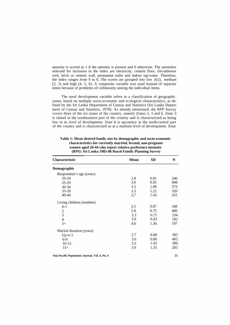
The principal independent variable is strength of fertility motivation. Thisvariable, which is called relative preference intensity (RPI), is based on twoquestions intended to assess how strongly respondents felt about having or nothaving another child.

Women who answered “yes” to the question: “Do you want to have any/another child sometime?” were then asked: “Would you say that your desireto have children/more children is not very strong, strong, or very strong?”Women who answered “no” to the first question were asked: “Would you saythat your desire not to have any more children is very strong, strong, or notvery strong?”

Responses were coded into relative preference intensity scores as follows:

Response RPI score

Want another childVery stronglyStronglyNot very strongly

Undecided

Want no more childrenNot very stronglyStronglyVery strongly

+3+2+1

0

-1-2-3

In our analysis of the determinants of contraceptive use, RPI is onlyone of several explanatory variables. The multivariate analysis includes addi-tional demographic and socio-economic variables because we wish to knowwhether RPI contributes to explanation over and above the effect of demo-graphic and socio-economic variables usually considered important in ana-lyses of the determinants of contraceptive use.

The control variables comprise variables known or thought to influencecontraceptive use. They include respondent’s age, number of living children,marital duration, age at first marriage, work status, a couple wealth index,and an areal measure of the level of economic and social development.

Most of these variables are self-explanatory; however, the couple wealthindex and the areal measure of development require further explanation. Thecouple wealth index is computed as a sum of household amenities, where a given


amenity is scored as 1 if the amenity is present and 0 otherwise. The amenitiesselected for inclusion in the index are electricity, cement floor, tile/asbestosroof, brick or cement wall, permanent toilet and indoor tap-water. Therefore,the index ranges from 0 to 6. The scores are grouped into low (0,l), medium(2, 3) and high (4, 5, 6). A composite variable was used instead of separateitems because of problems of collinearity among the individual items.

The areal development variable refers to a classification of geographiczones, based on multiple socio-economic and ecological characteristics, as de-fined by the Sri Lanka Department of Census and Statistics (Sri Lanka Depart-ment of Census and Statistics, 1978). As already mentioned, the RFP Surveycovers three of the six zones of the country, namely Zones 2, 3 and 6. Zone 3is inland in the southeastern part of the country and is characterized as beinglow in its level of development. Zone 6 is upcountry in the north-central partof the country and is characterized as at a medium level of development. Zone

Table 1: Mean desired family size by demographic and socio-economiccharacteristics for currently married, fecund, non-pregnantwomen aged 20-44 who report relative preference intensity

(RPI): Sri Lanka 1985-86 Rural Family Planning Survey

Characteristic Mean SD N

Demographic

Respondent’s age (years)20-2425-2930-3435-3940-44

Living children (number)0-12345+

Marital duration (years)Up to 56-910-1515+

2.8 0.81 2463.0 0.95 4083.2 1.06 3733.3 1.21 3203.7 1.43 201

2.5 0.87 3492.8 0.75 4863.3 0.71 3343.9 0.93 1824.6 1.36 197

2.7 0.88 3833.0 0.86 4053.2 1.03 3863.9 1.35 283


(Table 1 - Continued)

Characteristic Mean SD N

Age at first marriage (years)Up to 1718-2021-2425+

Socio-economic

Respondent’s education (years)0-56-910+

Couple’s education (years)Both 0-5Both 6-9Both 10+Wife < husbandHusband < wife

Couple’s work statusWife-domestic/husband-farmerWife-domestic/husband-non-farmerWife-non-domestic/husband-farmerWife-non-domestic/husband-non-farmer

Couple’s wealth indexLowMediumHigh

Areal development levelLowModerateHigh

Overall

3.5 1.29 2973.3 1.13 4383.1 1.03 4852.8 0.94 327

3.5 1.24 5583.1 1.07 5092.9 0.91 481

3.6 1.24 2793.1 1.02 2552.8 0.91 3213.3 1.23 3923.1 0.99 287

3.53.03.63.1

387766158237

3.33.22.9

1.220.991.221.07

1.131.111.04

1.221.071.01

884442222

3.53.13.0

500489559

3.2 1.12 1,548

Notes: Numbers of cases (N) for some variables do not add to the total because ofmissing values;

SD = standard deviation.


2 is coastal in the neighbourhood of Colombo and is characterized as beinghigh in level of development. In this context, low, medium and high are com-parative designations, not absolute ones.

In its simplest form, the dependent variable, current contraceptive use,is dichotomous (1 if using, 0 otherwise). Therefore, logistic regression is usedto analyze the determinants of overall contraceptive use. In addition, use issubdivided into traditional methods and modern methods, in which case thedependent variable has three categories. For this part of the analysis, multi-nomial logistic regression is used.

Results

Bivariate analysis

We begin our analysis with an investigation of how desired family size(number of children) varies by respondent characteristics in this data set. Re-sults are shown in table 1, which shows that desired family size increases sub-stantially with age, number of living children and marital duration. Moreover,those who marry earlier tend to desire larger families. The more educationa woman has, the lower the desired family size. The tabulations by couple’seducation, when compared with the tabulations by the woman’s education,indicate that the husband’s education has only a very small effect on the wife’sdesired family size. Desired family size decreases with both wealth and thelevel of areal development.

Table 2 complements table 1 by showing the distribution of the sampleon each variable in table 1 as well as on contraceptive method and RPI. TheRPI variable is noteworthy in that the category for RPI = 0 contains only 18cases. These are women who disproportionately expressed fatalistic or “don’tknow” responses to the questions on strength of fertility motivation.

Table 3 shows contraceptive use rates for broad categories of methods,for the respondent characteristics in tables 1 and 2. Interestingly, overall use(the “traditional or modern” column) varies little by age, number of livingchildren (except for women with 0-1 child, who have a markedly lower rateof use), marital duration and age at first marriage. Education has a larger effect,with those with six or more years of education having markedly higher ratesof use than those with five or fewer years of education. Couple’s work sta-tus has a moderately large effect on use; couples where the husband has non-farm employment and the wife works outside the home have a markedly higherrate of use than couples where the husband is a farmer and the wife does notwork outside the home. Contraceptive use varies little by couple wealth. Itvaries somewhat more, but irregularly, by level of areal development.


Table 2: Demographic and socio-economic characteristics of currentlymarried, fecund, non-pregnant women aged 20-44 who report

relative preference intensity (RPI): Sri Lanka 1985-86Rural Family Planning Survey

Characteristic Percentage or mean N

Demographic

Respondent’s age (years)20-2425-2930-3435-3940-44Mean (SD)

Living children (number)0-12345+Mean (SD)

Marital duration (years)Up to 56-910-1515+Mean (SD)

Age at first marriage (years)Up to 1718-2021-2425+Mean (SD)

Socio-economic

Respondent’s education (years)0-56-910+Mean (SD)

15.9 24626.4 40824.1 37320.7 32013.0 201

31.4 (6.3)

22.5 34931.4 48621.6 33411.8 18212.7 197

2.7 (1.7)

24.7 38326.2 40524.9 38618.3 283

9.7 (6.3)

19.2 29728.3 43831.3 48521.1 327

21.3 (4.3)

36.0 55832.9 50931.1 481

6.9 (3.4)



Characteristic Percentage or mean N

Couple’s education (years)Both 0-5Both 6-9Both 10+Wife < husbandHusband < wifeMean for husband (SD)Mean for wife (SD)

Couple’s work statusWife-domestic/husband-farmerWife-domestic/husband-non-farmerWife-non-domestic/husband-farmerWife-non-domestic/husband-non-farmer



Contraception and fertility preference

Contraception currently usedNoneTraditionalModern temporary

Relative preference intensity-3-2-10123

18.0 27916.5 25520.7 32125.3 39218.5 287

7.4 (3.2)6.9 (3.4)

25.0 38749.5 76610.2 15815.3 237

57.1 88428.6 44214.3 222

32.3 50031.6 48936.1 559

29.5 45654.5 84416.0 248

24.3 37615.4 2398.9 1371.2 18

23.8 36915.6 24110.9 168

Notes: In the couple work status variable, “domestic” means “housewife” or “workingin the home”, numbers of cases (N) for some variables do not add to the totalbecause of missing values; SD = standard deviation,


Table 3: Percentage of women currently using contraceptive methods bydemographic, socio-economic and fertility preference (characteristics):

Currently married, non-pregnant, fecund women aged 20-44,Sri Lanka 1985-86 Rural Family Planning Survey

CharacteristicTradi-

Tradi- Modern tional or Notional temporary modern method

Demographic

Respondent’s age (years)20-2425-2930-3435-3940-44

54.9 13.849.3 21.151.2 17.260.6 12.861.2 11.4

68.7 31.370.3 29.768.4 31.673.4 26.672.6 27.4

Living children (number)0-12345+

48.4 10.955.8 19.659.0 16.557.1 15.952.3 15.7

59.3 40.775.3 24.775.5 24.673.1 26.968.0 32.0

Marital duration (years)Up to 56-910-1515+

50.755.157.855.1

16.715.816.115.6

67.4 32.670.9 29.173.8 26.270.7 29.3

Age at first marriage (years)Up to 1718-2021-2425+

56.6 17.952.3 16.251.8 18.459.9 10.7

74.4 25.668.5 31.570.1 29.970.6 29.4

Socio-economic

Respondent’s education (years)0-56-910+

50.5 15.655.6 18.958.0 13.5

66.1 33.974.5 25.571.5 28.5


(Table 3 -Continued)

CharacteristicTradi-

Tradi- Modern tional or Notional temporary modern method

Couple’s education (years)Both 0-5Both 6-9Both 10+Wife < husbandHusband < wife

Couple’s work statusWife-domestic/husband-farmerWife-domestic/husband-non-farmerWife-non-domestic/

husband-farmerWife-non-domestic/

husband-non-farmer



Fertility preference


Overall average

50.9 15.4 66.3 33.758.4 18.8 77.3 22.858.3 12.8 71.0 29.052.0 16.3 68.4 31.654.7 16.7 71.4 28.6

50.9 15.5 66.4 33.655.2 16.2 71.4 28.6

55.1

57.8 16.9 74.7 25.3

52.8 17.2 70.0 30.055.9 16.3 72.2 27.858.6 10.8 69.4 30.6

52.4 13.2 65.6 34.453.4 20.9 74.2 25.857.4 14.3 71.7 28.3

54.8 16.5 71.3 28.761.5 15.9 77.4 22.664.2 14.6 78.8 21.250.0 0.0 50.0 50.058.0 19.2 77.2 22.847.7 15.4 63.1 36.938.7 11.9 50.6 49.4

54.5 16.0 70.5 29.5

15.2 70.3 29.8

Note: Number of cases (N) for some variables may not add to the total because ofmissing values.


Use shows greater variation by RPI. If one ignores the category for whichRPI equals zero, use remains high at 71-78 per cent for RPI values rangingfrom - 3 to +1, and then drops off to 63 and 51 per cent for RPI values of2 and 3, representing a desire for another child that is either strong or verystrong. As mentioned previously, the category of RPI equals zero contains only18 cases. These are disproportionately women who gave fatalistic responsesregarding desire for another child. It is therefore not surprising that contra-ceptive use is comparatively low for these women. This category of womenalso showed a comparatively low rate of contraceptive use in the Nepal studycited previously (Retherford, Tuladhar and Thapa, 1988).

The separate columns for traditional methods and modern temporarymethods in table 3 are interesting in that they show that the overall increasein contraceptive use that occurs with more education and wealth is due toan increase in the use of traditional methods, not modern methods. Use ofmodern temporary methods actually decreases as education and wealth increase.Of course, these are bivariate relationships that may not hold up when othervariables are controlled, a question that will be returned to later.

Table 4: Zero-order correlations between current contraceptive use(dependent variable) and demographic, socio-economic and fertility

preference characteristics (independent variables): Currently married,non-pregnant, fecund women aged 20-44, Sri Lanka 1985-86

Rural Family Planning Survey

Current contraceptive use

Independentvariable Traditional

Modern Traditionaltemporary or modern

Respondent’s age .079** -.063**No. of living children .036 .009Marital duration .046* -.025Age at first marriage .027 -.058*Respondent’s education .0.51* -.007Couple wealth index .043* -.053*Areal development level .042* .010Relative preference intensity -.090*** -.012

.036

.046*

.030-.017.050*.004.054*

-.108**

Notes: * denotes p < .05; ** denotes p <.01; and *** denotes p <.001.

The independent variables were all treated as continuous for purpose of calcu-lations.


Table 4 extends the bivariate analysis by showing bivariate correlationcoefficients between contraceptive use and each of the independent variablesincluded in the previous tables. (For purposes of computing correlations, allvariables are treated as continuous, which means, for example, that the couplewealth variable takes on possible values of 1, 2, or 3.) A striking aspect of thistable is that for five out of the eight independent variables, there appears tobe a trade-off between modern temporary methods and traditional methods.For example, age is positively related to use of traditional methods, but ne-gatively related to use of modern temporary methods. A similar pattern isapparent for marriage duration, age at first marriage, education and the cou-ple wealth index.

Another striking feature of this table is that the correlations are verylow, reinforcing the impression of a remarkable uniformity in contraceptiveuse across demographic and socio-economic characteristics, already apparentfrom table 3. Of the independent variables considered, RPI shows the highestcorrelation with contraceptive use, at about 0.11 for all methods combined.Interestingly, table 3 shows that most of the systematic variation in use withRPI is due to traditional methods, not modem methods.

Table 5 shows the bivariate correlation matrix for the independent va-

Table 5: Zero-order correlations between demographic, socio-economic andfertility preference characteristics (independent variables): currently married,

non-pregnant, fecund women aged 20-44, Sri Lanka 1985-86Rural Family Planning Survey

Vari-able AGE LVC MRD AFM EDU CWI DEV RPI

AGE 1.000 .522*** .746*** .336*** -.038 .183*** .170*** -.434***LVC 1.000 .716*** -.288*** -.264*** -.073** -.095*** -.576***MRD 1.000 -.320*** -.215*** .042 -.058*** -.477***AFM 1.000 .286*** .202*** .282*** .098***EDU 1.000 .386*** .238*** .077**CWI 1.000 .248*** -.035DEV 1.000 -.073**RPI 1.000

Notes: * denotes p < .05; ** denotes p < .01; and *** denotes p <.001.

Age = respondent’s age; LVC = number of living children; MRD = marital dura-tion; AFM = age at first marriage; EDU = respondent’s education; CWI = cou-ple’s wealth index; DEV = areal development level; RPI = relative preferenceintensity. The variables were all treated as continuous for purposes of calculatingcorrelations.


riables. Age, number of living children, and marital duration correlate in therange of 0.5 to 0.7. RPI correlates with age, number of living children, andmarital duration in the range of -0.4 to -0.6. The other correlations in thetable tend to be considerably lower.

Multivariate analysis

The multivariate analysis begins with an analysis of contraceptive usewithout distinguishing particular methods. Thus, the dependent variable is1 if using any method of contraception, and 0 otherwise. An appropriate sta-tistical model is logistic regression.

The results of this analysis are shown in tables 6 and 7. In table 6, thenumber of living children, number of living children squared, age at first mar-riage, and woman’s education are entered as continuous independent variables.The quadratic term for number of living children is included because previousstudies have indicated that the relationship between contraceptive use andnumber of living children often resembles an inverted U. All remaining inde-pendent variables are treated as categorical and are represented in the under-lying logistic regressions by sets of dummy variables. Age and marital durationare excluded from the models because of collinearity with number of livingchildren.

Table 6 includes two alternative models, Iabelled Model 1 and Model2. Model 1 omits relative preference intensity (RPI), whereas Model 2 includesit. The remaining independent variables, treated here as control variables, areincluded in both models. The two-model design enables one to address thequestion of whether the control variables capture the effect of motivationalstrength on current use of contraception when motivational strength (RPI)is deleted from the model.

Table 6: Logistic regression estimates of odds ratios for current use ofcontraception, by demographic and socio-economic characteristics of

women: Sri Lanka 1985-86 Rural Family Planning Survey

Characteristic Model 1 Model 2

Number of living children

Number of living children squared

Age at first marriage

Woman’s education

34

1.590 ( 5.22) 1.376 ( 3.15)

.954 (-4.51) .967 (-3.23)

.986 (-0.99) .983 (-1.13)

1.043 ( 2.20) 1.042 ( 2.08)

Asia-Pacific Population Journal, Vol. 4, No. 4


Characteristic Model 1 Model 2

Couple work statusWife domestic, husband farmerWife domestic, husband non-farmerWife non-domestic, husband farmerWife non-domestic, husband non-farmer

Couple wealth indexLowMediumHigh

Areal development levelLowMediumHigh


R2

-2 log likelihoodModel containing intercept onlyFull modelDifferenceDegrees of freedomp-value for difference

1.0001.118 ( 0.76)1.184 ( 0.80)1.358 ( 1.56)

1.000.957 (-0.31).804 (-1.21)

1.0001.502 ( 2.72)1.268 ( 1.57)

.013 .031

18741827

4711

.000

1.0001.132 ( 0.82)1.420 ( 1.62)1.424 ( 1.77)

1.000.961 (-0.28).840 (-0.94)

1.0001.596 ( 3.06)1.213 ( 1.25)

2.025 ( 2.98)2.683 ( 3.96)2.887 ( 3.73)

.762 (-0.52)3.206 ( 5.59)1.542 ( 2.06)1.000

18741783

9117

.000

Notes: Sterilized women are excluded from the regressions. Odds ratios are calculatedas exp(b), where B is the corresponding logistic regression coefficient. (In thecase of living children, however, exp(B) in the table is not interpretable as anodds ratio, because of the quadratic term, as explained in the text.) t-ratios areshown in parentheses after odds ratios. (The t-ratios actually pertain to thelogistic regression coefficients that underlie the odds ratios.) The R2 statisticis somewhat similar to R2 ordinary least squares multiple regression, but itis calculated quite differently, and it cannot be used in tests of significancelike an ordinary R2 (Harrell, 1983). The p-values in the bottom row of thetable indicate that each model differs very significantly from a model contain-ing only the intercept term. The two models also differ significantly from eachother, at p <.001, as explained in the text.


Table 6 presents odds ratios instead of the underlying logistic regressioncoefficients, because odds ratios are easier to interpret. (Odds ratios are cal-culated from the underlying coefficients, B, as exp(B).) For example, theodds ratio of 1.043 for woman’s education means that the odds of using con-traception are increased by a multiplicative factor of 1.043 with each addi-tional year of education. The odds ratio of 0.986 for age at first marriage meansthat the odds of using contraception are decreased by a factor of 0.986 witheach one-year increase in age at first marriage. From these examples, it is evi-dent that, for continuous variables, an odds ratio is interpreted as the multi-plicative effect of a one-unit increase in the variable on the odds of using con-traception, holding constant other independent variables included in the model.

The interpretation of the table entries for number of living children isdifferent, because of the squared term. If the woman has, say, one living child,the effect of a one-child increase in the number of living children is to increasethe odds of using contraception by a factor of (1.590) (0.954) (2)(1) = 1.447.If the woman has five living children, the effect of a one-child increase in thenumber of living children is to decrease the odds of using contraception bya factor of (1.590) (0.954) (2) (5) = 0.993.

In the case of a categorical variable, the reference category has anodds ratio of 1.000, corresponding to an underlying logistic regression coef-ficient of zero. For example, in the case of the couple wealth index, the re-ference category is “low”. The “medium” category has an odds ratio of0.957, meaning that the odds of current use for those with medium wealthare 0.957 of the odds of current use for those with low wealth in the referencecategory. Similarly, the “high” category has an odds ratio of 0.804, meaningthat the odds of current use for those with high wealth are 0.804 of the oddsof current use for those with low wealth in the reference category.

Quantities in parentheses following the odds ratios are t-ratios. Theyare calculated from the corresponding underlying logistic regression coeffi-cients and their standard errors, which are not shown. A t-ratio greater thanabout 2 indicates that the odds ratio differs significantly from unity at the5 per cent level of significance.

The R2 statistic in table 6 is somewhat similar to R2 in ordinary least-squares multiple regression, in that it has a lower bound of zero and an upperbound of one. However, its sampling distribution is unknown, which makestests of its statistical significance impossible. The log likelihood statistics, towhich we shall return later, are used instead for significance testing.

We are primarily interested in Model 2 in table 6, since it includes RPI,which is our principal explanatory variable. Relative to the reference category


of RPI = 3, it is seen that the effect of smaller values of RPI on the odds ofcontraceptive use is large. For RPI values of 1, -1, -2 and -3, the odds of useare multiplied by factors ranging between 2 and 3. These are net effects aftercontrolling for the other independent variables in the model.

The category for RPI = 0 is an outlier with a very low odds ratio, which,however, is not statistically significant, owing to the very small number ofcases, only 18 women. Despite the lack of statistical significance, a low oddsratio is expected, given that women in this category disproportionately givefatalistic responses to questions on fertility motivation. A very low odds ratiofor the RPI = 0 category was also found in the Nepal study cited previously(Retherford, Tuladhar and Thapa, 1988).

The effect of the control variables on the odds of contraceptive usedo not differ much between Models 1 and 2, and they are mostly consistentwith the simple bivariate findings examined previously in table 3. Numberof living children tends to increase the odds of use, at least at lower numbersof living children. Age at marriage has a very slight negative effect, which isstatistically non-significant. Woman’s education has a positive effect whichis statistically significant at about the 5 per cent level. Couple wealth appearsto reduce the odds of contraception, but the effect is statistically non-signi-ficant. The level of economic and social development of one’s geographic zoneof residence tends to increase the odds of use, but the effect is statisticallysignificant only for medium relative to low level of development.

Table 7, which is calculated from Model 2 in table 6, has the advantageof being easier to interpret than table 6. Table 7 shows estimates of the pro-bability of using contraception by each independent variable, controlling for

Table 7 : Logistic regression estimates of the probability of usingcontraception by demographic and socio-economic characteristics of women:

Sri Lanka 1985-86 Rural Family Planning Survey(probabilities expressed as adjusted percentages)

Characteristic Adjusted percentage

Number of living children012468

60.166.771.375.875.168.8



Characteristic Adjusted percentage

Age at first marriage (years)15 73.720 72.125 70.330 68.5

Woman’s education (years)0 65.62 67.44 69.16 70.98 72.510 74.1

Couple work statusWife domestic, husband farmer 68.4Wife domestic, husband non-farmer 71.1Wife non-domestic, husband farmer 75.5Wife non-domestic, husband non-farmer 75.6

Couple wealth indexLow 72.4Medium 71.5High 68.7

Areal development levelLow 67.0Medium 76.4High 71.1

Relative preference intensity-3 70.5-2 76.0-1 77.30 47.41 79.12 64.53 54.1

Notes: Adjusted values of the probability of use, P (expressed as a percentage), werecalculated from a multivariate logistic regression equation with independentvariables specified as in table 6. The effects of any given independent variable onuse were computed by holding the other independent variables constant attheir mean values in the entire sample.


the remaining independent variables by holding them constant at their meanvalues in the sample. The estimated probabilities are presented in the form ofadjusted percentages, where “adjusted” means that remaining independentvariables are held constant at their means.

Table 7 shows that number of living children tends to increase contra-ceptive use up to about four living children and to decrease it at higher numbersof living children. These effects are highly statistically significant, as seen pre-viously in table 6. Thus, the results show the inverted U-shaped pattern foundin many earlier studies (see, for example, Cleland, Little and Pitaktepsom-bati, 1979). The causation underlying this pattern is unclear for the womenwith higher numbers of living children. Because these women are nearing theend of their reproductive age, they may perceive themselves as no longer fe-cund. They may also be more traditional in their views and may be more like-ly to view contraception as inappropriate behaviour.

Table 7 shows that age at first marriage has a very small negative effecton contraceptive use, seen previously in table 6 to be statistically non-signifi-cant. Woman’s education increases contraceptive use, from about 66 per centfor women with no education to about 74 per cent for those with 10 years ofeducation. Couple work status tends to increase contraceptive use, but theeffects are statistically non-significant, as seen previously in table 6. Couplewealth tends to reduce use, but again the effects are statistically non-signifi-cant. A medium as opposed to a low level of areal development boosts usefrom 67 to 76 per cent.

The contrasts are greater by level of RPI, the main variable of interesthere. For RPI categories with adequate numbers of cases, use varies from 54per cent for RPI = 3 (very strongly wants another child) to 79 per cent forRPI = 1 (not very strongly wants another child). Use levels are rather similarfor RPI values of 1, -1, -2 and -3. As mentioned previously, the categoryfor RPI = 0, which is based on only 18 cases, is an outlier, with a use rate of47 per cent.

We now return to the question of whether Models 1 and 2 in table 6differ significantly from each other. This test is based on the -2 log likeli-hood statistic. The difference between the two models in this statistic is dis-tributed as chi-square with degrees of freedom equal to the difference betweenthe two models in the number of coefficients to be estimated. We see that1,827 - 1,783 = 44 with 17 - 11 = 6 degrees of freedom differs significantlyfrom zero at p< .001, which is highly significant. Thus the effects of RPI oncontraceptive use are not captured to any great extent by the backgroundvariables when RPI is deleted from the model. R2 is very low in both models,reflecting the fact that contraceptive use tends not to vary much across the in-dependent variables.


Table 8: Multinomial logistic regression coefficients and p-values for choiceof contraceptive method: Sri Lanka 1985-86 Rural Family Planning Survey

CharacteristicContraceptive method

Modern Traditional

Number of living children .668 ( 3.66) .253 ( 2.44)

Number of living children squared -.081 (-3.52) -.026 (-2.48)

Age at first marriage -.047 (-2.15) -.009 (-0.56)

Woman’s education .047 ( 1.71) .041 ( 2.03)


0. 0..112 ( 0.53) .117 ( 0.74).282 ( 0.91) .387 ( 1.71).366 ( 1.32) .318 ( 1.52)


0. 0.-.137 (-0.69)-.590 (-2.08)

-.007 (-.047)-.084 (-0.44)

Areal development levelLow 0. 0.MediumHigh

.889 ( 4.16) .328 ( 2.05)

.310 ( 1.38) .134 ( 0.83)

Relative preference intensity-3-2-10 - -123

.556 ( 1.58) .751 ( 3.00)

.688 ( 1.86) 1.065 ( 4.08)

.666 ( 1.60) 1.160 ( 3.92)

1.151 ( 3.69) 1.164 ( 5.30).388 ( 1.19) .440 ( 1.97)

0. 0.

Notes: The reference category for the dependent variable is non-use of contraception.In the body of the table, numbers in parentheses are t-ratios. There is no entryfor RPI = 0, because this cell contained only 18 cases, none of whom used mo-dern methods. Because no one used modern methods, MLOGIT would not run.Our solution to this problem was to omit the 18 cases for whom RPI = 0 andrerun MLOGIT without the category for RPI = 0.


Tables 8 and 9 extend Model 2 of the logistic regression analysis to amultinomial logistic regression analysis of the determinants of three cate-gories of contraceptive use: modern, traditional and no method. Because oddsratios are less meaningful in multinomial logistic regression than in simplebinary logistic regression, table 8 presents multinomial logistic regressioncoefficients instead of odds ratios. Also shown are t-ratios, which providean indication of level of statistical significance. Table 9, which is derived fromtable 8, shows expected probabilities of use of each method by each indepen-dent variable, again controlling for the other independent variables in the modelby setting them at their means. We shall restrict discussion to table 9, sinceit is easier to interpret than table 8.

In table 9, use of modern methods tends to rise with number of livingchildren, then to fall at larger family sizes. But use of traditional methodsincreases at least up to eight children, which is the largest family size con-sidered in the table. This finding supports the earlier hypothesis that olderwomen tend to be more traditional than younger women in their attitudesabout contraception.

Earlier, in the binary logistic regression analysis, the effects of age at mar-riage on use were found to be statistically non-significant. In the multinomiallogistic regression analysis in tables 8 and 9, however, age at first marriagehas a statistically significant negative effect on use of modern methods anda statistically non-significant positive effect on the use of traditional methods.This anomalous finding indicates that women who tend to be more modernin their marriage behaviour, by marrying late, tend to be more traditional intheir use of contraception.

Table 9 : Multinomial logistic regression estimates of the probabilities of usingspecified methods of contraception: Sri Lanka 1985-86 Rural Family

Planning Survey (probabilities expressed as adjusted percentages)

CharacteristicContraceptive method

Modern Traditional No method

Number of living children012468

8.2 51.9 40.012.3 54.3 33.416.1 55.4 28.619.5 56.5 24.015.7 58.9 25.47.9 59.9 32.2



Characteristic Contraceptive methodModern Traditional No method

Age at first marriage (years)15202530

Woman’s education (years)0246810



Areal development levelLowMediumHigh


19.2 54.6 26.216.2 55.8 28.013.6 56.7 29.711.3 57.2 31.4

13.7 51.5 34.814.2 52.9 32.914.7 54.2 31.015.2 55.5 29.315.7 56.7 27.516.3 57.9 25.9

14.915.415.216.9

17.015.210.7

12.021.014.6

14.813.812.7-

19.115.113.2

53.6 31.555.6 29.160.7 24.258.2 24.9

55.3 27.756.3 28.457.8 31.5

55.3 32.755.4 23.656.3 29.1

55.5 29.762.0 24.264.3 22.9- -

59.7 21.249.1 35.940.6 46.2

Notes: Adjusted values of the probability of use, P (expressed as a percentage), werecalculated from multinomial logistic regression equations with variables specifiedas in table 8. The effects of any given variable on method-specific use werecomputed by holding the other independent variables constant at their meanvalues in the entire sample. The category for RPI = 0 was omitted from theMLOGIT run for this table; see note to table 8.


This pattern is not observed, however, in the case of education. Themore education a woman has, the more likely she is to use both modern me-thods and traditional methods. However, the positive effect of education onuse of modern methods is not statistically significant at the 5 per cent level,whereas the positive effect of education on use of traditional methods is sta-tistically significant.

The anomalous finding for age at marriage reappears in the case of cou-ple wealth. Couple wealth has a statistically significant negative effect on useof modern methods, and a statistically non-significant positive effect on useof traditional methods. By contrast, level of areal development has an erraticeffect on use of modern methods and only a small, statistically non-significantpositive effect on use of traditional methods.

The effect of RPI, controlling for the other independent variables, isgreater for traditional use than for modern use. Indeed, the effect of RPI onmodern use is statistically significant only for RPI = 1, as shown in table 8.In contrast, the effects of RPI on traditional use tend to be considerably larg-er and highly statistically significant. In table 9, which shows this pattern moreclearly than does table 8, rates of use of modern methods by RPI range from15 to 19 per cent, whereas rates of use of traditional methods by RPI range from41 to 64 per cent. As in the binary logistic regressions, the percentage usingtraditional methods tends to be comparatively low, at 40-49 per cent for RPIvalues of 3 and 2 and considerably higher, at 56-64 per cent for RPI values of 1,-1, -2 and -3. The category RPI = 0 is omitted from this analysis for reasonsexplained in the footnote to table 8.

Conclusion

The picture that emerges from this analysis is that this comparativelyhomogeneous rural Sinhalese sample shows remarkably uniform rates of con-traceptive use across demographic and socio-economic variables. Rates of con-traceptive use are high and indicate that the contraceptive revolution is wellon its way to completion. Rates of contraceptive use would be even higherhad it been possible to include sterilized women, who were excluded becausethey were not asked the questions on strength of fertility motivation. Uniform-ly high rates of contraceptive use towards the end of fertility transition arenot unexpected in culturally homogenous populations. Such populations tendto show a convergence of differential fertility towards the end of the fertilitytransition (Retherford, 1985).

The analysis shows that neither the strength of motivation variable (re-lative preference intensity, or RPI) nor the control variables account for muchof the variability in contraceptive use. The effects of RPI on contraceptiveuse are nevertheless substantial and statistically significant. Rates of contra-


ceptive use are uniformly high among women who either do not want anotherchild or who want another child but do not feel very strongly about it. Theyare considerably lower, but still fairly high, among those who feel stronglyor very strongly that they want another child. The effects of RPI are strongerfor use of traditional methods of contraception than for use of modern me-thods of contraception. The fact that the rates are still fairly high for thosewho strongly want another child indicates widespread use of family planningfor birth spacing. The effects of the RPI variable hardly change when demo-graphic and socio-economic background variables are controlled, indicatingthat the effect of RPI on contraceptive use operates largely independentlyof the background variables.

The exclusion of sterilized women from the analysis introduces someselection on the dependent variable of contraceptive use. This exclusion intro-duces bias, but the bias is conservative in that the effects of RPI on use ofmodern methods of contraception would probably have been larger had itbeen possible to include sterilized women. Presumably, most of these womenfeel very strongly that they do not want another child.

References

Caldwell, J., K.H.W. Gaminiratne, P. Caldwell, S. De Silva, B. Caldwell, N. Weeraratneand P. Silva (1986). “The role of traditional methods of fertility control in SriLanka,” Studies in Family Planning, No. 18, pp. l-21.

Cleland, J.G., R.J.A. Little and P. Pitaktepsombati (1979). Illustrative Analysis: Socio-Economic Determinants of Contraceptive Use in Thailand. Scientific Reports No. 5(London, World Fertility Survey).

Hanushek, E.A. and J. E. Jackson (1977). Statistical Methods for Social Scientists. (NewYork, Academic Press).

Harell, F.E. (1983). “The LOGIST Procedure,” in SUGI Supplemental Library User’sGuide, 1983 Edition, (Cary, North Carolina, SAS Institute Inc), pp. 181-202.

Maddala, G.S. (1983). Limited-dependent and Qualitative Variables in Economics, (Cam-bridge, Cambridge University Press).

Pindyck, R.S. and D.L. Rubinfeld (1981). Economic Models and Economic Forecasts,(New York, McGraw-Hill).

Retherford, R.D. (1985). “A theory of marital fertility transition,” Population StudiesNo. 39, pp. 249-268.

traceptive use in Nepal,” Asian and Pacific Population Forum, vol. 2, Nos. 1-2,, J. Tuladhar and S. Thapa (1988). “Strength of fertility motivation and con-

pp. 5-12, 30-32.

Salford Systems (1988). The MLOGIT Procedure, (San Diego, Calif., Salford Systems).Photocopied documentation for computer program.

Sri Lanka Department of Census and Statistics (1978). World Fertility Survey Sri Lanka1975, First Report, (Colombo, Ministry of Plan Implementation).

44 Asia-Pacific Population Journal, Vol. 4, No, 4

Trends in Fertilityand Mortality in Fiji

Based on the 1986 Census

Fiji has undergone a ripid transitionin fertility and mortalityover the last two decades

By Bhakta B. Gubhaju and Naibuka Navunisaravi*

Fiji is made up of about 332 islands in the south-west Pacific. About ahundred of the islands are usually inhabited; most of the remaining islandsare used for temporary residence and for occasional plantation. Fiji has a longhistory of census taking: although the first census was taken in 1879, it was onlya very rough head count. A more comprehensive census was taken in 1881;

* The authors of this article are Bhakta B. Gubhaju, Research Fellow at the GraduateProgramme in Demography, National Centre for Development Studies, the AustralianNational University, Canberra, and Naibuka Navunisaravi, Acting Deputy Secretary,Ministry of Finance, Fiji. The former worked as UNFPA Expert in Fiji between April1988 and April 1989 to analyse the 1986 census of Fiji; the latter was GovernmentStatistician/Census Commissioner at the time the analysis of the 1986 census of Fijiwas carried out.


this census, in fact, inaugurated the series of decennial censuses which continueduntil 1921, after which there was, however, a break in this series. The nextcensus was not conducted until 15 years later, in 1936. From then on thecensuses have been conducted every 10 years; the last census took place in1986.

According to the 1986 census the population of Fiji was 715,375. Itconsists of two major ethnic groups, the indigenous Melanesian population,referred to in this article as Fijians, and the population who are of Indian origin,referred to as Indians. Apart from Fijians and Indians, there are Europeans,Chinese and other Pacific islanders, who form a small proportion of the totalpopulation. The 1986 census indicated that 48.7 per cent were Indians, 46per cent Fijians, with the remaining 5.3 per cent comprising other groups.The 1976-1986 intercensal rate of population growth was 2 per cent per annum,with Fijians increasing at 2.4 per cent and Indians increasing at 1.8 per cent.

The main objective of this article is to present the estimates of fertilityand mortality based on the 1986 census of Fiji. In some instances, comparativeestimates from the 1966 and 1976 censuses are also presented.

The population of Fiji comprises two major ethnic groups, the indigenousMelanesians and those of Indian origin, such as these women waiting for serviceat a family planning clinic. (Photograph courtesy of the Fiji Ministry of Informa-tion)


Methodology

In the Fiji censuses, direct data on deaths of individuals have not beencollected, so it is not possible to compute the crude death rate and age-specificdeath rates from the census data.

However, alternative data are gathered in the censuses which allow theapplication of indirect techniques to estimate infant and child mortality, adult-hood mortality and the construction of life tables. For example, the report-ing of children ever born and surviving by age of women has been used toestimate infant and child mortality by Brass-type methods.

Similarly, information on survivorship of respondent’s father and mo-ther at the time of enumeration has been used to estimate the adult survivor-ship probabilities of males and females respectively. Linkages of informationon childhood and adulthood mortality, in turn, have been employed by meansof the Brass logit linkage method to construct life tables for males and females.

Unlike mortality, the current fertility measures are directly obtained frominformation on the date of birth of the last child to women aged 15 yearsand over. In addition, the Fiji censuses also gathered information on the relation-ship of mothers with their own children.

These data provided a unique opportunity to estimate fertility trendsfor the past 15 years preceding the census by the application of the own-chil-dren method (Cho, 1973).

The estimated fertility and mortality rates based on census data arecompared with the corresponding data obtained from the Ministry of Healthand Vital Registration. Since most of the fertility and mortality rates are in-directly estimated, it is important to know the quality of census data usedfor the purpose of this article, because the estimates obtained from indirecttechniques are subject to the quality of age reporting.

The quality of the Fiji census data has been evaluated and it was foundthat for the 1986 census data the Myers’ Blended Index was 1.4, Whipple’sIndex was 105 for males and 106 for females and the United Nations Age-SexAccuracy Index was well below 20. These indices indicate that the age-sex datacollected in the Fiji censuses are highly accurate (Bureau of Statistics, 1989).

The following sections will present the estimates of mortality and fer-tility based on the indirect techniques. (Methodologies employed for esti-mating the mortality and fertility rates are discussed in Bureau of Statistics,1989).


Results

Mortality

Crude death rate

It was stated previously that the census data do not provide informationon deaths; however, deaths registered by the Registrar General and Ministry ofHealth independently provide annual crude death rates. It should be noted thatthe death rates obtained from the Registrar General are based on date of registra-tion of events while those of the Ministry of Health are based on date of occur-rence. However, both of these sources reveal that the crude death rate in Fijihas reached a fairly low level. The rates based on the registration data tend tofluctuate between 4.6 and 6.6 per thousand during the period 1980-1985,while the rates given by the Ministry of Health have shown a fairly regulardecline, from 5.7 in 1980 to 5.2 in 1984 (Bureau of Statistics, 1985 ; Ministryof Health, 1984).

Infant and child mortality

Infant and child mortality rates are obtained by applying Brass (1975)and Trussell (1975) methods to data on children ever born and surviving by ageof women. It is important to note that these methods of estimating childhoodmortality are based on the assumption that fertility and child mortality haveremained constant for the recent past. The fact that fertility and childhoodmortality have in fact been declining in Fiji may present biased estimates.The modification of this method, whereby it can be applied to a populationexperiencing a linear decline in mortality, has been presented by Feeney (1976;1980). For the purpose of this article, the Brass, Trussell and Feeney methodshave been applied to child survivorship data for Fijians, Indians and for thetotal population of Fiji. Coale and Demeny West Model Life Tables have beenused to select the appropriate multipliers (Coale and Demeny, 1966). Alter-natively, infant mortlaity rates obtained from deaths registered by the RegistrarGeneral and Ministry of Health and those estimated from the life tables basedon the Brass method of linkages between childhood and adult mortality arealso presented for comparison.

Table 1 presents the probabilities of dying before reaching exact childhoodages for Fijians, Indians and the total population by males and females; theseestimates are based on the Brass and Trussell methods. Also shown are infantand child mortality rates corresponding to the childhood mortality ratesestimated by the Trussell method and calendar year referring to the rates. Itcan be seen from this table that except for the estimates based on the age group15-19 years, all other estimates provided by the Brass and Trussell methodsare close to each other.


The infant mortality rates based on the age group 15-19 are known to bebiased for two basic reasons. First, these methods assume that the risk of a childdying is invariant to a woman’s age or child’s birth order. In practice, however,children born to women of 15-19 years of age experience higher mortality thanthe average. Second, the number of children born and dead pertaining to thisage group is usually small and rates estimated are subject to random fluctuations.For these reasons, infant mortality estimates based on the 15-19 age group ofwomen are generally disregarded.

Since the Brass and Trussell estimates of childhood mortality are close toeach other, the Trussell estimates are considered for converting childhoodmortality into infant mortality rates. The infant mortality rates thus estimatedare also associated with calendar years. There has been a continuous declinein infant mortality rates over the years and this decline has been experiencedby the Indians and Fijians. It is also apparent that the higher male than femaleinfant mortality rates observed in this table conform with the general patternof sex differentials in infant mortality. Indians, in general, are also found tohave higher infant mortality than Fijians, a finding that accords with the resultsof the Ministry of Health. According to the Ministry of Health, the higherinfant mortality rate among Indian children, particularly during the neonatalperiod, is associated with the high incidence of low birth weight (Ministry ofHealth, 1984).

Trussell’s estimates of infant mortality rates corresponding to the year1984 are 31 per thousand for males and 27 per thousand for females, but itwill be shown that these rates are, in fact, overestimations of the rates prevailingin the country. It has been observed that, in the case of declining mortality, theBrass-type methods tend to overestimate the current mortality levels (Kralyand Norris, 1978, 551).

Table 2 depicts infant mortality rates estimated by the Feeney methodbased on the 1986 census data. It shows a continuous fall in infant mortalityover the years. In addition, the trends in infant mortality estimated by theFeeney method derived from the 1976 and 1986 census data are plotted infigures 1-3. It is evident that, irrespective of sex and ethnic origin, infantmortality has experienced a continuous decline over the past 20 years betweenthe 1960s and 1980s.

It should be noted, however, that the rates estimated by the Feeneymethod are well below those estimated by the Trussell method. For example,the infant mortality rates for Fiji for the period 1984 are 24 for males and20 for females. It is therefore suggested that in the case of declining childhoodmortality, the Trussell method tends to overestimate the level of child mortalitycurrently prevailing in the country. In view of the observed trends in infant


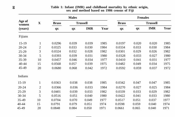
Table 1: Infant (IMR) and childhood mortality by ethnic origin,sex and method based on 1986 census of Fiji

Age ofwomen(years)

X Brass

qx

Males

Trussell

qx IMR Year

Brass

qx

Females

Trussell

qx IMR Year

Fijians

15-1920-2425-2930-3435-3940-44

45-49

Indians

15-19 1 0.0363 0.038 0.038 1985 0.0342 0.047 0.047 198520-24 2 0.0366 0.036 0.033 1984 0.0270 0.027 0.025 198425-29 3 0.0401 0.039 0.033 1982 0.0339 0.033 0.029 198230-34 5 0.0516 0.051 0.040 1980 0.0422 0.041 0.033 198035-49 10 0.0704 0.070 0.049 1977 0.0517 0.051 0.037 197740-44 15 0.0791 0.079 0.051 1974 0.0598 0.059 0.040 197445-49 20 0.0848 0.084 0.050 1971 0.0661 0.065 0.040 1971

1 0.0296 0.039 0.039 1985 0.0197 0.020 0.020 19852 0.0325 0.033 0.030 1984 0.0334 0.033 0.030 19843 0.0324 0.032 0.028 1982 0.0301 0.029 0.026 19825 0.0393 0.039 0.031 1980 0.0328 0.033 0.027 1980

10 0.0457 0.046 0.034 1977 0.0410 0.041 0.031 197715 0.0568 0.057 0.039 1975 0.0482 0.049 0.034 197520 0.0680 0.068 0.042 1972 0.0592 0.059 0.037 1972

Total

15-1920-2425-2930-3435-3940-44

45-49

1235

101520

0.0341 0.039 0.039 1985 0.0263 0.022 0.022 19850.0340 0.034 0.031 1984 0.0295 0.029 0.027 19840.0366 0.037 0.032 1982 0.0317 0.031 0.027 19820.0458 0.045 0.036 1980 0.0374 0.037 0.030 19800.0579 0.058 0.041 1977 0.0461 0.046 0.034 19770.0678 0.068 0.045 1974 0.0533 0.0530.0762 0.076 0.046 1971 0.0618 0.062

Table 2: Infant mortality rates (IMR) by ethnic origin and sexusing Feeney Method based on 1986 census of Fiji

0.036 19740.038 1971

Age ofwomen(years)

Fijians Indians Total

Male Female Male Female Male Female

IMR Year IMR Year IMR Year IMR Year IMR Year IMR Year

20-24 23 1984 24 1984 26 1984 18 1984 24 1984 20 198425-20 20 1982 19 1982 25 1982 21 1982 23 1982 19 198230-34 23 1980 18 1980 30 1980 24 1980 27 1980 21 198035-39 21 1977 18 1977 36 1977 24 1977 28 1977 21 197740-44 25 1974 20 1974 38 1974 27 1974 32 1974 23 197445-49 29 1971 24 1971 37 1971 27 1971 33 1971 25 1971

s

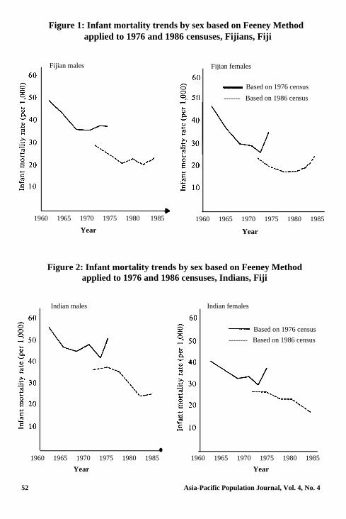
Figure 1: Infant mortality trends by sex based on Feeney Methodapplied to 1976 and 1986 censuses, Fijians, Fiji

Fijian males

%.%.

‘.“/-.. .’./

1960 1965 1970 1975 1980 1985

Year

Fijian females

- Based on 1976 census

------- Based on 1986 census

%, ,#’*--. ,/-._----

1960 1965 1970 1975 1980 1985

Year

Figure 2: Infant mortality trends by sex based on Feeney Methodapplied to 1976 and 1986 censuses, Indians, Fiji

Indian males Indian females

- Based on 1976 census

-------- Based on 1986 census

l1960 1965 1970 1975 1980 1985 1960 1965 1970 1975 1980 1985

Year Year


Figure 3: Infant mortality trends by sex based on Feeney Methodapplied to 1976 and 1986 censuses, Fiji

Total males

-mm.

‘*.---7

‘Le.--

1960 1965 1970 1975 1980 1985

Year

Total females

- Based on 1976 census_----. Based on 1986 census

1960 1965 1970

Year

1975 1980 1985

mortality, it seems reasonable to infer that the rates estimated by the Feeneymethod are a closer approximation of the infant mortality rates for Fiji.

The infant mortality rates estimated indirectly from the Trussell andFeeney methods are compared with those estimated from the life tables con-structed using the Brass method of linkages between child survivorship pro-babilities. These are set out in table 3. The detailed methodologies for thelife table construction are contained in Bureau of Statistics, 1989.

It should be noted that the infant mortality rates estimated by the Trusselland Feeney methods presented in this table are based on the reporting of child-ren ever born and surviving to women aged 20-24 years; these rates, therefore,refer to about 2.5 years before the census. Also presented for comparisonare infant mortality rates obtained from deaths registered by the RegistrarGeneral and Ministry of Health.

It can be seen from this table that the infant mortality rates based onlife table methods are only a few points lower than those of the Feeney method.It is also encouraging to note that the estimates based on the Feeney and lifetable methods are remarkably close to the rates obtained from the Ministryof Health. Additionally, the rates obtained from deaths registered by the Re-gistrar General are also not too far off the other estimates.


Table 3: Trends in infant mortality rates (IMR)a/, b/, c/ by ethnic origin and sexestimated by various methods

Ethnicoriginand sex

1966

Tf/ Fg/

FijiansMaleFemaleTotal

IndiansMaleFemale - -Total

TotalMaleFemale - -Total

-i/ -

58 50 - - - - - -

- -

79 69 - - - - - -

- -

71 61

1976 1986 1984

Tf/ Fg/ LTh/

46 38 36.8 30 23 19.6- - 41 35 28.2 30 24 18.8

59 50 41.346 38 32.6

54 45 -45 37 -- - - - - -

33 26 23.025 18 19.6- -

31 24 22.7 -27 20 19.1 -

Tf/ Fg/ LTh/ MOHd/ RGe/

- 17.7- 13.0

22.1 -

- 22.1- 16.2

22.7 -

19.014.2

22.5 -

Notes: aJ IMRs for the Trussell and Feeney methods are based on the reporting of children ever born and surviving to women aged

Notes: a/ IMRs for the Trussell and Feeney methods are based on the reporting of children ever born and surviving to women aged 20-24 years.b/ IMRs by males and females could not be estimated for 1966 census because questions on children ever born and surviving

were not asked for boys and girls separately.c/ IMRs obtained from registration data are based on infant deaths registered in 1984.d/ MOH: Ministry of Health.e/ RG: Registrar General.f/ T: Trussell Method.g/ F: Feeney Method.h/ LT: life table method.i/ -: Estimates not available.

However, the fact that the rates are calculated on the basis of the dateof registration of events rather than the date of occurrence makes the estimateshighly questionable, because some of the infant deaths registered in a givenyear may have occurred in the same year and some in the preceding years.For these reasons, infant mortality rates obtained from the Registrar Generalcannot be taken as authentic. Thus, the infant mortality rates estimated eitherby the Feeney or life table methods or those provided by the Ministry of Healthwould closely represent the rates prevailing in Fiji. Hence, on the basis of thisevidence we may conclude that there has been a substantial decline in theinfant mortality rate in Fiji, both among Fijians and Indians, between 1966and 1986. The infant mortality rates for Fiji around the period 1984 are below25 per thousand live births, with slightly higher rates among Indians than amongFijians.

Adult mortality

In the preceding section, infant and childhood mortality rates wereestimated indirectly by using data on survivorship of children by age of women.Similarly, indirect estimates of adulthood survivorship probabilities can bemade if the data on survivorship of fathers and mothers by age of respondentsare collected in the census. In the 1986 Population Census of Fiji, questionswere asked about each member of the household on the survival status of realfather and mother at the time of enumeration. The method derived by Brassand Hill (1973) converts the proportion of respondents with surviving fatheror surviving mother to yield a plausible estimate of adulthood survivorshipprobabilities. This method has been applied to the 1986 census data to estimatethe adulthood survivorship probabilities for males and females separately forFijians and Indians. The results are presented in table 4. (See United Nations,1983 for elaboration of the method and Bureau of Statistics, 1989 for applica-tion of the method.)

The estimated probabilities of surviving presented in table 4 reveal thatfemales, in general, have higher probabilities of surviving than males; this patternis followed for both Fijians and Indians. It is also apparent that the mortalitylevel corresponding to different age groups of respondents is not constant.The higher the age group of respondents used for estimating survivorship pro-babilities, the earlier is the time referring to these estimates. Apparently, adult-hood mortality rates have been shown to be continuously declining over time,so it becomes necessary to affix the time to which these estimates refer.

A method proposed by Brass and Bamgboye (1981) has been employedto estimate the actual time to which each estimate refers (see United Nations,1983 for elaboration of the method). The results are presented in table 4. It isevident from this table that the level of mortality has been increasing over time


Table 4: Estimates of conditional adult survivorship probabilities by ethnic origin and sexbased on 1986 census of Fiji

Agegroup(years)

Paternal mortality Maternal mortality

N Proportion 1 (35+N) Mortality Ref. Proportion 1 (25+N) Mortality Ref.with father 1 (32.5) level date with mother 1 (25) level date

alive alive

Fijians

15-1920-2425-2930-34

g 35-492 40-442 45-49;PFi; Indians2.Cl 15-19; 20-243[u 25-29; 30-34; 35-39z 40-44PP 45-49

20 0.9110 0.8775 20.45 1977 0.9559 0.9497 20.42253035404550

20253035404550

0.8456 0.7917 19.62 1976 0.9210 0.9156 19.750.7506 0.6660 18.52 1974 0.8709 0.8654 19.000.6344 0.4899 16.64 1973 0.7894 0.7846 17.830.4803 0.2916 14.13 1971 0.6767 0.6654 16.330.3298 0.1409 12.76 1970 0.5389 0.5193 15.090.2073 0.0437

0.8908 0.8147 16.96 19770.8058 0.6993 15.37 1975 0.9363 0.9186 19.95 19760.7015 0.5747 14.71 1973 0.8764 0.8534 18.37 19740.5996 0.4094 13.15 1972 0.7977 0.7671 17.02 19730.4748 0.2822 13.64 1970 0.6952 0.6513 15.79 19720.3669 0.1311 12.11 1969 0.5766 0.5148 14.92 19710.2514

0.4095 0.3603 14.32

0.9673 0.9572 21.05 1977

0.3067 0.3524 13.98

197719761974197319721971

D Totalg.

2 15-192.2 20-240” 25-29Di 30-34g 35-39i 40-442 45-49

-2P

ozP

20 0.9007 0.8460 18.67 1977 0.9616 0.9534 20.73 197725 0.8240 0.7435 17.42 1975 0.9291 0.9180 19.91 197630 0.7241 0.6160 16.48 1974 0.8741 0.8599 18.71 197435 0.6159 0.4516 15.01 1972 0.7944 0.7763 17.42 197340 0.4802 0.2790 13.47 1971 0.6883 0.6596 16.11 197245 0.3507 0.1351 12.38 1969 0.5607 0.5199 15.11 197150 0.2313 0.0353 0.4287 0.3572 14.18

Table 5: Expectations of life at birth by ethnic origin and sex,Fiji, 1976-1986

1976 1986Sex

Fijians Indians Fijians Indians Total

Male 60.7 59.5 63.1 59.6 61.0Female 63.9 62.4 65.3 65.1 65.2

Note: The 1976 estimates are obtained from: Zwart, F.H.A.G., Report on the Census of the Population 1976, Volume II: Demo- graphic Characteristics, Parliament of Fiji, Parliamentary Paper No. 43, Bureau of Statistics, Suva, 1979.

Fijian farmers at work - male adulthood mortality among the Melanesian population is substantially lower than among those of Indian background.

which means that adulthood mortality has been declining. This table alsosuggests that there is not any meaningful difference in female adulthoodmortality between the Fijians and Indians, but male adulthood mortality issubstantially higher among Indians than among Fijians. This means that a lowerproportion of Indian than Fijian males survive to adult ages.

Expectations of life at birth

Expectation of life at birth is one of the most important indices ofmortality which reflects the overall health standards of a given population. Itis generally estimated by constructing life tables, for which age-specific deathrates or the probabilities of surviving by age are the basic data required. Age-specific death rates are commonly obtained from the vital registration datawhile the probabilities of surviving by age can be estimated through indirectmeans. In the case of Fiji, although age-specific death rates are available fromdeaths registered by the Registrar General, for the aforementioned reasons,these data are not very reliable for constructing the life tables. An attempt wasmade, however, to construct life tables based on these age-specific death rates,but the expectations of life at birth derived from these data were unbelievablyhigh. This also gives an indication of under-registration of deaths. An alternativemethod was to estimate expectations of life at birth indirectly. One of the indi-rect ways often used to construct life tables is through the intercensal survivalmethod, which is strictly limited to closed populations with accurate censusestaken five or ten years apart. In the case of Fiji, although the censuses can beconsidered to be fairly accurate, the assumption of a closed population does nothold. The population of Fiji, especially that of Indians, has been substantially


affected by migration; hence, the application of this method to construct lifetables was ruled out.

It was then finally decided to apply the Brass method of linkages of childsurvivorship probabilities with conditional adult survivorship probabilities toconstruct life tables. This method not only has advantages in constructinglife tables but also has a built-in procedure to graduate the range of survivorshipprobabilities (United Nations, 1983). For this purpose, child survivorship pro-babilities, 1(2), 1(3) and 1(5) estimated by the Trussell method were linkedwith conditional adult survivorship probabilities to construct life tables formales and females separately for Fijians, Indians and the total population(Bureau of Statistics, 1989).

Table 5 presents the expectations of life at birth estimated from the 1986census; also shown are the estimates based on the 1976 census report (Zwart,1979). This table reveals that the overall expectation of life at birth for Fijireached 61 years for males and 65.2 years for females in 1986. The expectationsof life at birth are somewhat higher for Fijians than for Indians; this is muchmore evident for males than for females. The Fijian life expectancy at birthincreased from 60.7 years in 1976 to 63.1 years in 1986 for males, while forfemales it increased from 63.9 years to 65.3 years during the same period. Incontrast, there appears to be very little increase in the expectation of life at birthfor Indian males, which increased from 59.5 years in 1976 to 59.6 years in1986*, but for Indian females it increased relatively more, from 62.4 to 65.1years during the same period,. In general, it can be inferred that the healthstandards of Fiji, as measured by the expectations of life at birth, improvedsignificantly between 1976 and 1986.

Fertility

Crude birth rate

Crude birth rates are calculated from the information on births to womenaged 15 years and above during the year preceding the 1986 census; theserates are presented in table 6. Also presented are crude birth rates obtainedfrom the censuses of 1966 and 1976 and those obtained from the RegistrarGeneral and the Ministry of Health. According to the 1986 census, the crudebirth rate for Fiji is 27 per thousand population, with the Fijians having highercrude birth rates at 30 per thousand than the Indians at 24.3 per thousand.The rates obtained from the Registrar General for the year 1985 are 27.9 forFiji as a whole, 29.2 for Fijians and 26.7 for Indians. The Ministry of Health’sfigure for Fiji is 30.0 per thousand pertaining to the same year; and the rates

* It is difficult to explain the ethnic differentials in mortality between Fijians and In-dians; however, one can speculate that part of the variance may be due to differentdietary habits, life-styles and related socio-cultural factors among the two ethnic groups.


Table 6: Crude birth rates by ethnic origin and source,Fiji, 1966-1986

Source Year Fijians Indians Total

Population Census 1966Report 1976a/

39.3 39.91976 31.6 30.9

Ministry of Healthb/ 1976 31.2 30.0 30.3" " " 1985 33.5 27.2 30.0

Registrar Generalc/ 1985 29.2 26.7 27.9

Censusd/ 1986 30.0 24.3 27.0

Sources: a/ Zwart, F.H.A.G., Report on the Census of the Population 1976, Volume II:Demographic Characteristics, Parliament of Fiji, Parliamentary Paper No. 43,Bureau of Statistics, Suva, 1979;

b/ Ministry of Health and Social Welfare, Annual Report for the Year 1984,Parliament of Fiji, Parliamentary Paper No. 1 of 1986;

c/ Bureau of Statistics, Vital Statistics in Fiji (Statistics of Births, Deaths andMarriages), A Report for the Year 1985, Suva, 1986; and

d/ Current estimates based on 1986 census.

are 33.5 and 27.2 per thousand for Fijians and Indians, respectively. It is alsonoteworthy that the crude birth rates estimated from the 1976 census andMinistry of Health for the period 1976 are close to each other.

Table 6 also presents the trends in crude birth rate, and shows thatthere was a faster decline in crude birth rate among both the Fijian and Indianpopulations between 1966 and 1976. During this period, the Fijian crudebirth rate declined from 39.3 to 31.6 per thousand while the correspondingdecline for Indians was from 39.9 to 30.9 per thousand respectively. However,between 1976 and 1986, the Fijian crude birth rate declined very little, from31.6 to 30 per thousand, while the Indian crude birth rate declined from30.9 to 24.3. It is clear that the Indian crude birth rate was consistently de-clining from 1966 to 1986, while there has been a slow-down in recent yearsin the pace of decline in the crude birth rate among Fijians.

Age-specific and total fertility rates

The preceding section examined the fertility level of Fiji in terms ofcrude birth rate. Because of its limitation, i.e. the rates are subject to changesin age structure of the population under study, a more refined measure offertility is warranted to depict the true level of fertility. The age-specific andtotal fertility rates are the most practical measures of current fertility. These


rates are readily obtained from the information on live births which occurredduring the year preceding the census. The rates, therefore, represent the pe-riod immediately preceding the census. Alternatively, the age-specific and totalfertility rates can be estimated indirectly for the 1.5 years preceding the census,provided the census collects additional information on the relationships ofmothers with their own children. Fortunately, Fiji made an effort in the censusto collect data on the relationships of mothers with their own children; thisfacilitated the application of the own-children method to estimate fertilitytrends in Fiji for the 15 years preceding the census.

The input data required for the application of the own-children tech-nique is the single-year age distribution of population under 16 years of ageby the age of their own mothers; these are tabulated in the 1986 census re-port (see Bureau of Statistics, 1988). Based on this method, the age-specificfertility rates are estimated by reverse projection of enumerated childrento the time of their birth and the female population to each of the years pre-

Figure 4: Trends in total fertility rate (TFR) based on own-childrenmethod by ethnic origin, 1966-1986

1966 67 68 69 70 71 72 73 74 75 76 77 78 79 80 81 82 83 84 85 86

Years

Notes: 0 , 0 = Based on 1976 census;

X , -̂ = Based on 1986 census.


Table 7: Trends in total fertility rates (TFR) by ethnic origin and source, Fiji, 1976-1986

Year Own Own Vital Census Own Own Vital Census

Fijians Indians TotalOwn Vital Census

child. child. reg. 1986 child. child. reg. 1986 child. reg. 19861976a/ 1986b/ c/ d/ 1976a/ 1986b/ c/ d/ 1986b/ c/ d/

1966 5.6 5.41967 5.2 4.81968 5.2 4.51969 5.0 4.51970 5.0 4.21971 4.6 4.11972 4.5 4.4 3.8 3.9 4.11973 4.5 4.4 3.9 3.9 4.21974 4.4 4.5 3.6 3.7 4.11975 4.5 4.5 3.6 3.7 4.11976 4.3 4.3 3.5 3.7 4.01977 4.4 3.5 3.91978 4.4 3.6 4.01979 4.6 3.7 4.21980 4.7 3.8 4.21981 4.5 3.7 4.11982 4.5 3.5 4.01983 4.5 3.3 3.81984 4.4 3.2 3.71985 4.1 3.4 2.9 2.8 3.4 3.11986 4.1 3.9 2.8 2.6 3.4 3.2

Notes: a/ Zwart, F.H.A.G., Report on the Census of Population 1976, Volume II: Demographic Characteristics, Parliament of Fiji,Parliamentary Paper No. 43, Bureau of Statistics, Suva, 1979.

b/ Current estimates based on own-children method.c/ Bureau of Statistics, Vital Statistics in Fiji (Statistics of Births, Deaths & Marriages): A Report for the Year 1985, Suva, 1986.d/ Current estimates based on births occurring during one year preceding the census.

ceding the census. For the purpose of the reverse projection of enumeratedchildren to the time of their birth and the female population, the life tablesconstructed from the 1986 census have been used (Bureau of Statistics, 1989).

The advantage of this method is that it does not depend upon any assump-tion about fertility trends and is not very sensitive to assumptions about recentchanges in the level of mortality (United Nations, 1983). Therefore, only oneset of mortality levels has been used in the reverse projection of the popu-lation and mortality is assumed to have remained constant during the periodstudied.

Detailed outputs of age-specific and total fertility rates for the periodbetween 1972 and 1986, obtained by using the software package, EASWESPOP:Fertility Estimates Program (East-West Center, 1987), are contained inBureau of Statistics (1989) while the summary results are presented in table7 and displayed in figure 4. The fertility trends based on the own-children me-thod applied to the 1976 census (Zwart, 1979) are also presented for compa-rison.

The results show that these two data sets present remarkably close esti-mates and they almost overlap for the period 1972-1976. Among Fijians, thetrends in fertility reveal that the total fertility rate was 5.6 in 1966; it expe-rienced a continuous decline and reached 4.3 in 1976. It then slowly increasedup to 4.7 in 1980, remained constant at 4.5 between 1982 and 1984 and de-clined steadily to 4.1 in 1986. The rates estimated by the own-children me-thod are also compared with those obtained from other sources. The totalfertility rate of 3.4 for 1985 obtained from the Registrar General is lower thanother estimates. For example, the total fertility rates estimated by the own-children method and the one obtained directly from the census data, bothreferring to the year 1986, are 4.1 and 3.9, respectively.

It can also be seen from this table that compared with Fijians, Indianshave experienced a much faster decline in fertility. The total fertility rate of5.4 observed among Indians in 1966 declined to 3.8 in 1972; it then remainedalmost unchanged, or fluctuated between 3.5 and 3.9 during the period 1972-1981 ; it was not until after 1981 that Indian fertility resumed its pace ofdecline. The total fertility rate has now come down to less than 3 children perwoman. The other estimates also tend to put the Indian total fertility ratebetween 2.6 and 2.8 for the year 1986.

It is also apparent from the above trends that the Fijian and Indian fert-lity rates were both high and similar in 1966: the total fertility rates were 5.6for Fijians and 5.4 for Indians. Both ethnic groups experienced a decline infertility over time, but it was much more noticeable among Indians than Fijians,with the result that the gap in fertility between Fijians and Indians started


Figure 5 : Age-specific fertility rates (ASFR) per thousand Fijians, 1966 -1986

340320 - ,a/' '\

/' \300 -

280260240

8220

O"200; 180a 160g 140

4 12010080

6040

200 4

Age 15-19 20-24 25-29 30-34 35-39 40-44 45-49years

0 1966 x 1976 -̂ 1986

Table 8: Age-specific fertility rates (per thousand) by ethnic origin,Fiji, 1966-1986

Agegroup(years)

Fijians Indians

1966a/ 1976a/ 1986b/ 1966a/ 1976a/ 1986b/

15-19 55 42 62 95 53 6220-24 287 237 211 329 244 20725-29 323 257 227 299 218 16230-34 238 174 171 203 113 8035-39 148 99 106 122 49 2940-44 59 37 40 48 14 1045-49 7 4 11 6 1 5

Notes: a/ Zwart, F.H.A.G., Report on the Census of the Populution 1976, Volume II:Demographic Characteristics, Parliament of Fiji, Parliamentary Paper No. 43,Bureau of Statistics, Suva 1979; and

b/ Current estimates based on own-children method.


Figure 6: Age-specific fertility rates (ASFR) per thousand Indians, 1966-1986

340320300

280260240

220g 200_

180& 160

g 140q 120

100

80

60

4020

0

Age 15-19 20-24 25-29 30-34 35-39 40-44 45-49years

El 1966 x 1976 -̂ 1986

widening. Eventually in 1986, the Fijian total fertility rate was 4.1 as opposedto 2.8 for Indians, a difference of more than one child between Fijians andIndians.

It is not only the total fertility rate but also the age pattern of fertilitythat is different between Fijians and Indians. Table 8 and figures 5 and 6 presentthe age-specific fertility rates for Fijians and Indians for the 1966, 1976 and1986 censuses. Apparently, the fertility decline was observed for every agegroup between 1966 and 1976 for both the Fijians and Indians.

It is interesting that fertility among Fijians seems to have gone up between1976 and 1986 in the younger age group, 15-19 years, and the older age group,35-49 years. It is only the middle age group, 20-34 years, which appears to haveexperienced some decline in fertility between these periods. But in contrast,among Indians - except for the age groups 15-19 and 45-49 years - all agegroups of women experienced a noticeable decline in fertility. The pattern offertility shows that among Fijians, peak fertility occurred among women aged25-29 years, while among Indians the peak occurred among women aged 20-24years. These patterns prevailed during all the censuses of 1966, 1976 and 1986.


References

Brass, W. (1975). Methods for Estimating Fertility and Mortality from Limited andDefective Data, (The Carolina Population Center, University of North Carolina atChapel Hill).

and K.H. Hill (1973). “Estimating Adult Mortality from Orphanhood.”Proceedings of the International Population Conference, Liege, 1973, Vol. 3, (Liege,IUSSP), pp. 111-123.

and E.A. Bamgboye (1981). The Time Location of Reports of Survivor-ship: Estimates of Maternal and Paternal Orphanhood and the Ever-Widowed”.Working Paper No. 81-1, (London, Centre for Policy Studies, London School ofHygiene and Tropical Medicine).

Bureau of Statistics (1985). Vital Statistics in Fiji (Statistics of Births, Deaths andMarriages), A Report for the Year 1985, (Suva, Fiji).

(1988). Report on Fiji Population Census 1986, Volume 4 - Fertility andMortality. Parliament of Fiji, Parliamentary Paper No. 10 of 1988, (Suva, Fiji).

(1989). Report on Fiji Population Census, 1986: Analytical Report on theDemographic, Social and Economic Characteristics of the Population, (Suva, Fiji).

Cho, Lee-Jay (1973). “The Own-Children Approach to Fertility Estimation: An Elabora-tion.” Proceedings of the International Population Conference, Liege, 1973, Vol. 2,(Liege, IUSSP), pp. 263-280.

Coale, A.J. and P. Demeny (1966). Regional Model Life Tables and Stable Populations,(Princeton, Princeton University Press).

East-West Center (1987). EASWESPOP: Fertility Estimates Program, User’s Manual,Version 1.1, (Honolulu, East-West Center, East-West Population Institute).

Feeney, G. (1976). “Estimating Infant Mortality Rates from Child Survivorship Databy Age of Mother.” Asian and Pacific Newsletter, vol. 3, No. 2, pp. 12-16.

(1980). “Estimating Infant Mortality Trends from Child SurvivorshipData.” Population Studies, vol. 34, No. 1, pp. 109-128.

Kraly, E.P. and D.A. Norris (1978). “An Evaluation of Brass Mortality Estimates UnderConditions of Declining Mortality.” Demography, vol. 15, No. 4, pp. 549-557.

Ministry of Health and Social Welfare (1986). Annual Report for the Year 1984, Parlia-ment of Fiji, Parliamentary Paper No. 1 of 1986, (Suva, Fiji).

Trussell, T.J. (1975). “A Reestimation of the Multiplying Factors for the Brass Techniquefor Determining Childhood Survivorship Rates.“ Population Studies, vol. 29, No. 1,pp. 97-108.

United Nations (1983). Manual X: Indirect Techniques for Demographic Estimation,Department of International Economic and Social Affairs, Population Studies,No. 81, (New York, United Nations).

Zwart, F.H.A.G. (1979). Report on the Census of the Population 1976, Volume II:Demographic Characteristics, Parliamentary Paper No. 43, (Suva,Bureau of Statistics,Fiji).


Demographers’ Notebook

Population Conference

The International Union for the Scientific Study of Population (IUSSP)held its Twenty-first International Population Conference at New Delhi from20 to 27 September 1989. The Conference, which was organized at the in-vitation of the Indian Association for the Study of Population (IASP), wasopened by India’s Prime Minister Rajiv Ghandi.

The numerous papers presented at the Conference were published undervarious headings in three volumes. Volume 1: patterns of fertility change inAsia, demography of China, data collection systems in South Asia, popula-tion growth policies in South-east Asia, social structure and fertility change,emerging issues in fertility control, fertility analysis, the conditions of childsurvival, and biomedical and demographic aspects of health. Volume 2: non-traditional approaches to demographic data collection; indirect methods ofdemographic analysis; international migration systems, processes and policies;megacities: trends, issues and policies; changing patterns of migratory flows;population and rural development; population and long-term perspectivesin pre-modern economic development; and changing family structure andlabour markets in industrialized countries. Volume 3: demographic aspectsof planning for health, education and employment; aging: economic and so-cial aspects; changing family structures and life courses; marriage systems anddemographic trends in developed countries; demographic issues in developedcountries; case studies in anthropological demography; peopling of the conti-nents; and priority needs for the development of the discipline of demography.

In addition to the many papers that were presented at the Conference,new members of the Council of the Union were selected for the period 1989-1993. Among them were Massimo Livi-Bacci of Italy who replaces WilliamBrass as President; John C. Caldwell of Australia as Vice-President; and AllenG. Hill of the United Kingdom of Great Britain and Northern Ireland replacingGeorges Tapinos as Secretary General and Treasurer. New members of theCouncil are Dragana Avromov of Yugoslavia, J.A. Magna de Carvalho of Bra-zil, Monica Das Gupta of India, Charlotte Hohn of the Federal Republic ofGermany, Jacques Legare of Canada, John H. Pollard of Australia, RolandPressat of France and Saw Swee-Hock of Singapore.


Documents

China: Surplus Labour and Migration - · PDF fileChina: Surplus Labour and Migration ... which villages and small towns are encouraged to build small factories to ... often serve local