Embed Size (px)
Citation preview

c e p a l r e v i e w 1 1 0 • a u g u s t 2 0 1 3 189
Chile: subsidies, credit and housing deficit
Fernando Garcia de Freitas, Ana Lélia Magnabosco and Patrícia H. F. Cunha
ABSTRACT This article has two objectives: to analyse the effects of the housing subsidy on
access to credit and on real-estate investment; and to study the influence of those
relations in the Chilean experience. Following a review of the financing and subsidy
systems in Chile, a theoretical model is put forward to analyse the effect of subsidies
on housing credit and on the equilibrium of the real-estate market. The model offers
new perspectives on the role played by subsidies policy and the structure on which
the empirical research is based. The econometric analysis corroborates the two main
theoretical proposals, namely: access to the subsidy increases a family’s chances
of obtaining credit and reduces the number of families living in a housing-deficit
situation. The econometric results also help to interpret the trend of the housing
deficit in Chile.
KEYWORDS Housing, housing needs, housing subsidies, credit, econometric models, statistical data, housing finance, Chile
JEL CLASSIFICATION R21, R28, H53
AUTHORS Fernando Garcia de Freitas, National Services Confederation, Brazil. [email protected]
Ana Lélia Magnabosco, University of São Paulo, Brazil. [email protected]
Patrícia H. F. Cunha, Pontifical Catholic University of São Paulo, Brazil. [email protected]

c e p a l r e v i e w 1 1 0 • a u g u s t 2 0 1 3190
Chile: SubSidieS, Credit and houSing defiCit • fernando garCia de freitaS, AnA LéLiA MAgnAbosco And PAtríciA H. F. cunHA
In the mid-1970s, a far-reaching reform of the real-estate financing system was undertaken in Chile, with the explicit aim of boosting investments in homes and overcoming the housing deficit. Innovative mechanisms combining credits and subsidies were created, and these had an immediate effect on the market.
Apart from representing a satisfactory experience of real-estate financing and serving as a benchmark for other Latin American countries, the Chilean case provides a good empirical basis for an analysis of how a subsidies policy can affect economic agents’ decisions and the volume of real-estate investments —partly because it is a policy that has now been applied for many years, so its long-term effects can be observed. Moreover, the wide variety of home-purchase modalities available allow for a more effective evaluation of the relations that exist between subsidy, credit and income. Housing can be financed through subsidies, credit, self-financing without subsidies and, lastly, through a combination of credit and subsidies.
This article is organized in five sections following this introduction. Section II describes the Chilean financing model and the main subsidy programmes; section III sets forth a theoretical model to analyse how subsidies influence housing credit and affect equilibrium in the real-estate market. That model offers new perspectives on the role played by subsidies policy and provides the structure on which the empirical research reported in the following sections is based. Section IV performs an econometric analysis to measure the influence of the subsidies on a family’s chances of obtaining housing credit, which, in addition to helping to interpret the Chilean experience, provides empirical elements that corroborate the proposed theoretical model. Section V describes the methodology for estimating the housing deficit in Chile, and provides details of the calculations, based on data obtained from the National Socioeconomic Survey (casen). The section also reports other econometric research inspired in the relations that exist between the variables that determine real-estate investment. The article concludes with a section offering final thoughts.
IIntroduction
IIsummary of housing policy in chile
Chilean housing policy has three dimensions: (i) the financing system; (ii) the subsidies policy; and (iii) the regulations governing construction and urban development. Each of those dimensions has evolved at a different rate over the last 50 years, displaying well-defined phases. This section reviews the housing-finance models, the subsidy policy and its interaction with credit —issues that provide the central focus of this article.1
1. Financing system
The history of housing finance in Chile in the twentieth century can be divided into three periods, identified by the financial intermediation instruments used to channel
1 For a broader historical view of Chilean housing policy, see Castillo and Hidalgo (2007); minvu (2007), and Brain, Cubillos and Sabatini (2007).
savings into real-estate investment: (i) up to 1959; (ii) from 1959 to 1976; and (iii) after 1976.
According to Morandé (1993), mortgage finance played a key part in Chilean financial intermediation policy in the first period. In the 1930s, mortgage bonds —instruments issued in pesos with nominal interest rates— grew to represent 50% of total bank lending. In the wake of the upsurge in inflation from 1940 onwards, however, the corresponding interest rates fell below the rate at which prices were rising and came to represent income transfers from investors to mortgage borrowers. The market was unable to resist, and the supply of credit in the system decreased sharply.
In 1959, the government solved the problem by creating tax incentives for both supply and demand, defined in Decree with Force of Law No. 2 of 1959 (dfl2). The innovation contained in the decree consisted of instituting a monetary-correction scheme for long-term

c e p a l r e v i e w 1 1 0 • a u g u s t 2 0 1 3
chile: subsidies, credit and housing deficit • fernando garcia de freitas, ana lélia Magnabosco and patrícia h. f. cunha
191
operations, thereby making it possible for investment and saving to coexist with high inflation rates.
In the same year, the National Saving and Loan System (sinap) was created. This played an important role in capturing saving through saving and loan associations; and it also revitalized housing activity and validated the system of readjustment indices, which formed the basis for the subsequent success of the new housing finance systems established from the 1970s onwards. The indexation of saving deposits and mortgage loans, which remains in force today, played a crucial role in eliminating inflationary risk and guaranteeing the supply of credit at lower cost.
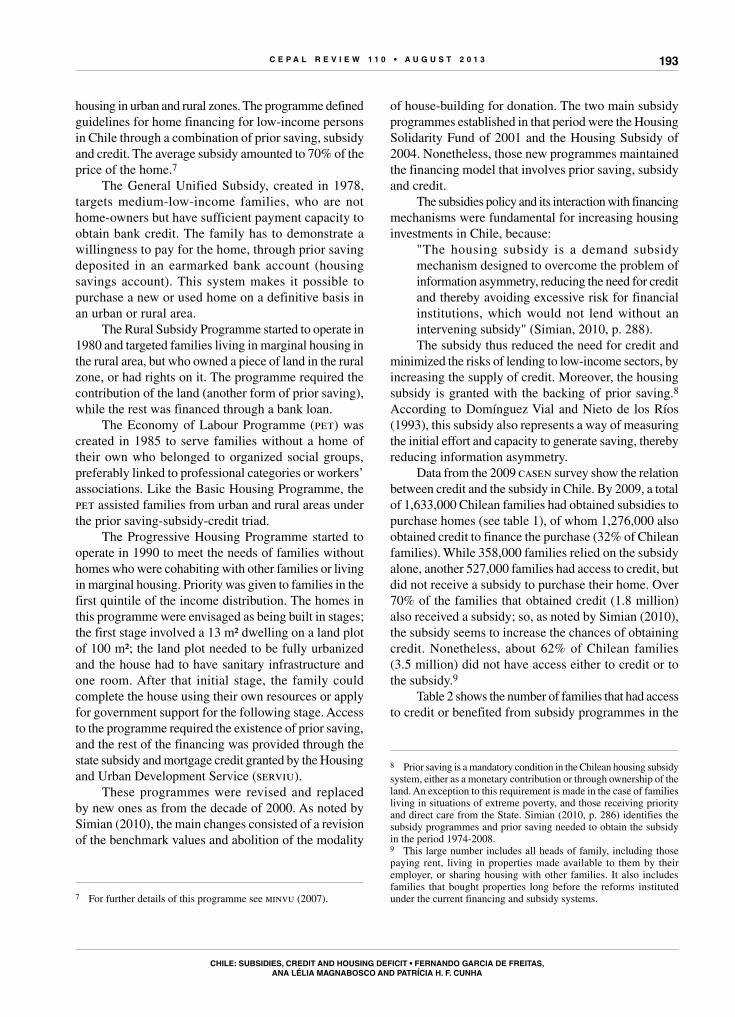
In the 1960s and early 1970s, the government introduced a wide-ranging subsidies policy to help low-income sectors purchase homes. Between 1960 and 1969, nearly 68,000 families received a subsidy to buy their own home, and the number grew to almost 150,000 between 1970 and 1979 (see figure 1). In just three years of that period, from 1970 to 1972, over 72,500 families received the subsidy.
The sinap lost momentum in the 1970s, however; and between 1974 and 1976, the number of housing units
financed per year (16,100) fell by 28% compared to the previous four years (22,400).2 That occurred because savings dwindled in the wake of the recession, and this was compounded by a loss of purchasing power among the population and political instability in the country. There was also a mismatch between investment and savings maturity periods, a problem previously encountered in the North American system.
In 1976, a new institutional framework was introduced through structural reforms to liberalize the economy, accompanied by economic stabilization measures. This resulted in a far-reaching reorganization of the capital market, which in turn had repercussions on financial intermediation and housing credit.
The social security reform implemented in late 1980 was another important factor which promoted the secondary securities market and channelled large amounts of long-term savings into real-estate financing. According to the Pensions Supervisor, the number of funded pension accounts grew rapidly following the
2 casen Survey 2009.
FIgurE 1
chile: total number of families with access to credit and the subsidy,a 1950-2009
10 4
80
67 9
00 149
974
326
979
514
784
510
390
13 9
51
87 7
34
180
880
323
397
529
700 60
5 49
2
0
100 000
200 000
300 000
400 000
500 000
600 000
700 000
1950-1959 1960-1969 1970-1979 1980-1989 1990-1999 2000-2009
Subsidy Credit
Source: prepared by the authors on the basis of the 2009 National Socioeconomic Survey.
a Includes social rental programmes.
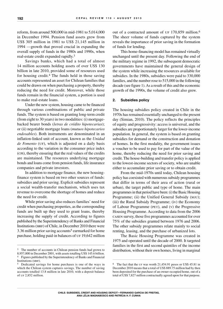
c e p a l r e v i e w 1 1 0 • a u g u s t 2 0 1 3192
Chile: SubSidieS, Credit and houSing defiCit • fernando garCia de freitaS, AnA LéLiA MAgnAbosco And PAtríciA H. F. cunHA
reform, from around 500,000 in mid-1981 to 5,014,000 in December 1994. Pension fund assets grew from uS$ 305 million in 1981 to uS$ 21,145 million in 1994 —growth that proved crucial in expanding the overall supply of funds in the 1980s and 1990s, when real-estate credit expanded rapidly.3
3 The number of accounts in Chilean pension funds had grown to 8,957,000 in December 2001, with assets totalling uS$ 145.6 billion.
Savings banks, which had a total of almost 14 million accounts holding assets of over uS$ 130 billion in late 2010, provided some of resources used for housing credit.4 The funds held in those saving accounts represented an asset for Chilean families that could be drawn on when purchasing a property, thereby reducing the need for credit. Moreover, while those funds remain in the financial system, a portion is used to make real-estate loans.
under the new system, housing came to be financed through various combinations of public and private funds. The system is based on granting long-term credit (from eight to 30 years) in two modalities: (i) mortgage-backed bearer bonds (letras de crédito hipotecarias); or (ii) negotiable mortgage loans (mutuos hipotecarios endosables). Both instruments are denominated in an inflation-linked unit of account, known as the Unidad de Fomento (uf), which is adjusted on a daily basis according to the variation in the consumer price index (cpi), thereby ensuring that the real values of the credits are maintained. The resources underlying mortgage bonds and loans come from pension funds, life insurance companies and private investors.
In addition to mortgage finance, the new housing-finance system is based on two other sources of funds: subsidies and prior saving. Explicit subsidies represent a social wealth-transfer mechanism, which uses tax revenue to overcome the shortage of homes and reduce the need for credit.
While prior saving also reduces families’ need for credit when purchasing properties, as the corresponding funds are built up they used to grant loans, thereby increasing the supply of credit. According to figures published by the Superintendency of Banks and Financial Institutions (sbif) of Chile, in December 2010 there were 3.36 million prior saving accounts5 earmarked for home purchase, holding paid-in balances of uf 19,642 million
4 Figures published by the Superintendency of Banks and Financial Institutions (sbif). 5 Dedicated savings for home purchases is one of the ways in which the Chilean system captures savings. The number of saving accounts totalled 13.8 million in late 2010, with a deposit balance of uf 2,852 million.
out of a contracted amount of uf 170,859 million.6 The sheer volume of funds captured by the system reveals the importance of prior saving in the formation of funds for lending.
This home-financing model has remained virtually unchanged until the present day. Following the end of the military regime in 1992, the subsequent democratic governments have maintained the general design of the system while increasing the resources available for subsidies. In the 1980s, subsidies were paid to 330,000 families, and the number rose to 515,000 in the following decade (see figure 1). As a result of this and the economic growth of the 1990s, the volume of credit also grew.
2. subsidies policy
The housing subsidies policy created in Chile in the 1970s has remained essentially unchanged to the present day (Simian, 2010). The policy reflects the principles of equity and progressivity: access is universal, and the subsidies are proportionately larger for the lower-income population. In general, the system is based on granting subsidies for demand or the construction and donation of homes. In the first modality, the government issues a voucher to be used to pay for part of the value of the home, thereby reducing the need for prior saving and credit. The house-building and transfer policy is applied to the lowest-income sectors of society, who are unable either to accumulate prior saving or to obtain credit.
From the mid-1970s until today, Chilean housing policy has coexisted with numerous subsidy programmes that differ in terms of their area of action (rural or urban), the target public and type of home. The main programmes in that period have been: (i) the Basic Housing Programme; (ii) the unified general Subsidy (sgu); (iii) the rural Subsidy Programme; (iv) the Economy of Labour Programme (pet), and (v) the Progressive Housing Programme. According to data from the 2006 casen survey, those five programmes accounted for over 75% of the subsidies granted between 1976 and 2006. The other subsidy programmes relate mainly to social renting, leasing, and the purchase of urbanized lots.
The Basic Housing Programme was created in 1975 and operated until the decade of 2000. It targeted families in the first and second quintiles of the income distribution, without their own homes, living in marginal
6 The fact that the uf was worth 21,454.91 pesos or uS$ 45.81 in December 2010 means that a total of uS$ 889.75 million had by then been deposited for the purchase of an owner-occupied home, out of a total of uS$ 7,827 million contractually agreed upon for that purpose.
c e p a l r e v i e w 1 1 0 • a u g u s t 2 0 1 3
chile: subsidies, credit and housing deficit • fernando garcia de freitas, ana lélia Magnabosco and patrícia h. f. cunha
193
housing in urban and rural zones. The programme defined guidelines for home financing for low-income persons in Chile through a combination of prior saving, subsidy and credit. The average subsidy amounted to 70% of the price of the home.7
The general unified Subsidy, created in 1978, targets medium-low-income families, who are not home-owners but have sufficient payment capacity to obtain bank credit. The family has to demonstrate a willingness to pay for the home, through prior saving deposited in an earmarked bank account (housing savings account). This system makes it possible to purchase a new or used home on a definitive basis in an urban or rural area.
The rural Subsidy Programme started to operate in 1980 and targeted families living in marginal housing in the rural area, but who owned a piece of land in the rural zone, or had rights on it. The programme required the contribution of the land (another form of prior saving), while the rest was financed through a bank loan.
The Economy of Labour Programme (pet) was created in 1985 to serve families without a home of their own who belonged to organized social groups, preferably linked to professional categories or workers’ associations. Like the Basic Housing Programme, the pet assisted families from urban and rural areas under the prior saving-subsidy-credit triad.
The Progressive Housing Programme started to operate in 1990 to meet the needs of families without homes who were cohabiting with other families or living in marginal housing. Priority was given to families in the first quintile of the income distribution. The homes in this programme were envisaged as being built in stages; the first stage involved a 13 m² dwelling on a land plot of 100 m²; the land plot needed to be fully urbanized and the house had to have sanitary infrastructure and one room. After that initial stage, the family could complete the house using their own resources or apply for government support for the following stage. Access to the programme required the existence of prior saving, and the rest of the financing was provided through the state subsidy and mortgage credit granted by the Housing and urban Development Service (serviu).
These programmes were revised and replaced by new ones as from the decade of 2000. As noted by Simian (2010), the main changes consisted of a revision of the benchmark values and abolition of the modality
7 For further details of this programme see minvu (2007).
of house-building for donation. The two main subsidy programmes established in that period were the Housing Solidarity Fund of 2001 and the Housing Subsidy of 2004. Nonetheless, those new programmes maintained the financing model that involves prior saving, subsidy and credit.
The subsidies policy and its interaction with financing mechanisms were fundamental for increasing housing investments in Chile, because:
"The housing subsidy is a demand subsidy mechanism designed to overcome the problem of information asymmetry, reducing the need for credit and thereby avoiding excessive risk for financial institutions, which would not lend without an intervening subsidy" (Simian, 2010, p. 288).The subsidy thus reduced the need for credit and
minimized the risks of lending to low-income sectors, by increasing the supply of credit. Moreover, the housing subsidy is granted with the backing of prior saving.8 According to Domínguez Vial and Nieto de los ríos (1993), this subsidy also represents a way of measuring the initial effort and capacity to generate saving, thereby reducing information asymmetry.
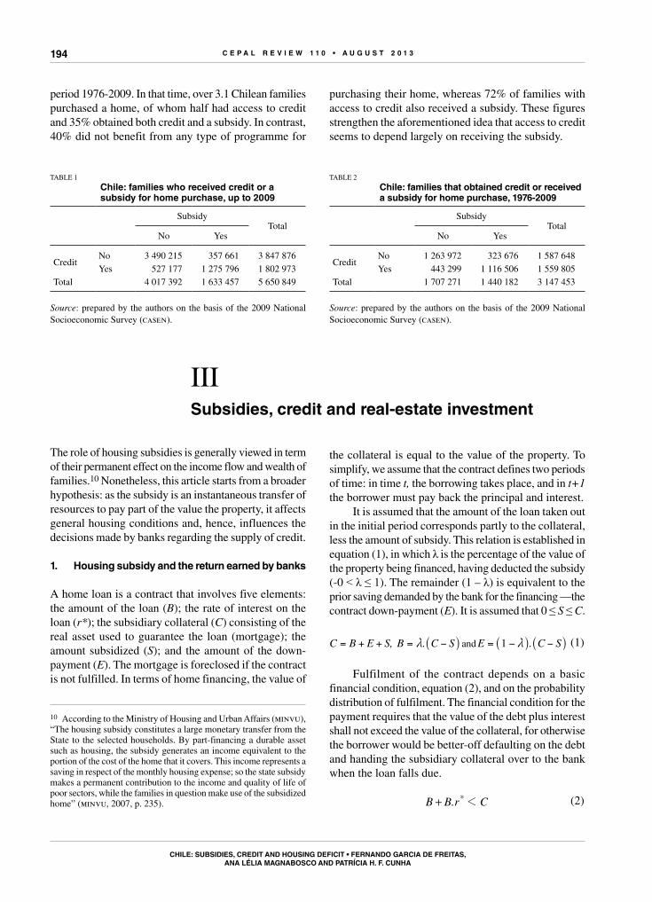
Data from the 2009 casen survey show the relation between credit and the subsidy in Chile. By 2009, a total of 1,633,000 Chilean families had obtained subsidies to purchase homes (see table 1), of whom 1,276,000 also obtained credit to finance the purchase (32% of Chilean families). While 358,000 families relied on the subsidy alone, another 527,000 families had access to credit, but did not receive a subsidy to purchase their home. Over 70% of the families that obtained credit (1.8 million) also received a subsidy; so, as noted by Simian (2010), the subsidy seems to increase the chances of obtaining credit. Nonetheless, about 62% of Chilean families (3.5 million) did not have access either to credit or to the subsidy.9
Table 2 shows the number of families that had access to credit or benefited from subsidy programmes in the
8 Prior saving is a mandatory condition in the Chilean housing subsidy system, either as a monetary contribution or through ownership of the land. An exception to this requirement is made in the case of families living in situations of extreme poverty, and those receiving priority and direct care from the State. Simian (2010, p. 286) identifies the subsidy programmes and prior saving needed to obtain the subsidy in the period 1974-2008.9 This large number includes all heads of family, including those paying rent, living in properties made available to them by their employer, or sharing housing with other families. It also includes families that bought properties long before the reforms instituted under the current financing and subsidy systems.
c e p a l r e v i e w 1 1 0 • a u g u s t 2 0 1 3194
Chile: SubSidieS, Credit and houSing defiCit • fernando garCia de freitaS, AnA LéLiA MAgnAbosco And PAtríciA H. F. cunHA
period 1976-2009. In that time, over 3.1 Chilean families purchased a home, of whom half had access to credit and 35% obtained both credit and a subsidy. In contrast, 40% did not benefit from any type of programme for
purchasing their home, whereas 72% of families with access to credit also received a subsidy. These figures strengthen the aforementioned idea that access to credit seems to depend largely on receiving the subsidy.
TABLE 1
chile: families who received credit or a subsidy for home purchase, up to 2009
Subsidy
TotalNo Yes
CreditNo 3 490 215 357 661 3 847 876Yes 527 177 1 275 796 1 802 973
Total 4 017 392 1 633 457 5 650 849
Source: prepared by the authors on the basis of the 2009 National Socioeconomic Survey (casen).
TABLE 2
chile: families that obtained credit or received a subsidy for home purchase, 1976-2009
Subsidy
TotalNo Yes
CreditNo 1 263 972 323 676 1 587 648Yes 443 299 1 116 506 1 559 805
Total 1 707 271 1 440 182 3 147 453
Source: prepared by the authors on the basis of the 2009 National Socioeconomic Survey (casen).
III subsidies, credit and real-estate investment
The role of housing subsidies is generally viewed in term of their permanent effect on the income flow and wealth of families.10 Nonetheless, this article starts from a broader hypothesis: as the subsidy is an instantaneous transfer of resources to pay part of the value the property, it affects general housing conditions and, hence, influences the decisions made by banks regarding the supply of credit.
1. Housing subsidy and the return earned by banks
A home loan is a contract that involves five elements: the amount of the loan (B); the rate of interest on the loan (r*); the subsidiary collateral (C) consisting of the real asset used to guarantee the loan (mortgage); the amount subsidized (S); and the amount of the down-payment (E). The mortgage is foreclosed if the contract is not fulfilled. In terms of home financing, the value of
10 According to the Ministry of Housing and urban Affairs (minvu), “The housing subsidy constitutes a large monetary transfer from the State to the selected households. By part-financing a durable asset such as housing, the subsidy generates an income equivalent to the portion of the cost of the home that it covers. This income represents a saving in respect of the monthly housing expense; so the state subsidy makes a permanent contribution to the income and quality of life of poor sectors, while the families in question make use of the subsidized home” (minvu, 2007, p. 235).
the collateral is equal to the value of the property. To simplify, we assume that the contract defines two periods of time: in time t, the borrowing takes place, and in t+1 the borrower must pay back the principal and interest.
It is assumed that the amount of the loan taken out in the initial period corresponds partly to the collateral, less the amount of subsidy. This relation is established in equation (1), in which λ is the percentage of the value of the property being financed, having deducted the subsidy (-0 ˂ λ ≤ 1). The remainder (1 – λ) is equivalent to the prior saving demanded by the bank for the financing —the contract down-payment (E). It is assumed that 0 ≤ S ≤ C.
, . .C B E S B C S E C S1m m= + + = − = − −_ _ _i i iand (1)
Fulfilment of the contract depends on a basic financial condition, equation (2), and on the probability distribution of fulfilment. The financial condition for the payment requires that the value of the debt plus interest shall not exceed the value of the collateral, for otherwise the borrower would be better-off defaulting on the debt and handing the subsidiary collateral over to the bank when the loan falls due.
.B B Cr* 1+ (2)

c e p a l r e v i e w 1 1 0 • a u g u s t 2 0 1 3
chile: subsidies, credit and housing deficit • fernando garcia de freitas, ana lélia Magnabosco and patrícia h. f. cunha
195
Provided condition (2) is satisfied, the contract will be fulfilled or otherwise depending on the interest conditions and the resources available to the borrower. Let p be the probability of fulfilment of the financing contract: in period t + 1 each contract has a probability p of being paid and (1 - p) of not being paid. The probability p depends on the resources of the families (w) and the interest rate on the home financing, as shown in equation (3).
f , , ,p w r p 0 1* d= _ i 7 A (3)
A rise in the interest rate on the home loan is assumed to reduce the probability of fulfilment of the contract, whereas an increase in the wealth of the families raises this.11 The second derivatives are assumed positive.
and,r
p
r
pwp
w
p0 0 0 0* *2
2
2
2
2
2
2
2
2
2
2
21 2 2 2 (4)
The return to the banks depends on the parameters of the contract and the probability of fulfilment. If the borrower respects the contract, the bank pays out the amount lent and receives the same amount back plus the loan interest. If the borrower does not respect the contract, the bank loses the amount lent but receives the subsidiary collateral. Figure 2 shows the return to the banks each case.
FIgurE 2
possible return from the real-estate loan
B C–t 1
++
p
1 – p
. .B r B r C S rB B * * *tm− + + = _ i. .= −
Source: prepared by the authors.
To simplify, it is assumed that the value of the collateral in t + 1 is equal to its value in t, in other
11 It should be remembered that, by definition, p is constrained to the interval between 0 and 1. When p attains the value 1, the derivative of p with respect to w becomes zero.
words, neither the increase in the value of the property through time, nor the depreciation rate (δ) in the period, are taken into account.
C C Ct t1 = =+ (5)
Considering the two possibilities, fulfilment or not fulfilment, the bank’s expected return (Π) is a function of the loan interest rate, the amount of the subsidy and the amount lent.
, , . . .r S B p B r p C B1* *P = + − −_ _ _i i i (6)
The banks’ expected rate of return is defined as the expected return divided by the amount lent:
, , , , . .r S B r S B B p r p C B1 1* * *t P= = + − −_ _ _ `i i i j (7)
The banks are assumed to be profit-maximizers, so the interest rate on the loan will be that which maximizes the bank’s expected return, as proposed by Stiglitz and Weiss (1981). Formulating the derivative of the banks’ expected rate of return with respect to r*, and taking account of equation (3), gives:
. .
rp r p p C B 1*
*r r2
2t= + − −' ' ` j
This relation may be greater or less than zero (0) depending on the interest rate on the loan. given that p>0, p'r<0 , as assumed in equation (4), and C ≥ B, when the interest rate tends to zero (0) the derivative is positive. In contrast, when r* tends to infinity, the derivative is negative.
lim limyr r0 0* *
r r0* *2 2 2 22 1t t
" "3 and lim limyr r0 0* *
r r0* *2 2 2 22 1t t
" "3
Identifying the interest rate that maximizes the banks’ rate of return requires setting the aforementioned derivative to zero (0). That condition assumes that:
B p1 1= − − =or. .p r p C r BC
p
p* *r r
r
− −' ''
` j (8)
Consequently, there is a maximum interest rate that is positive. If the interest rate is greater than r*, the
c e p a l r e v i e w 1 1 0 • a u g u s t 2 0 1 3196
Chile: SubSidieS, Credit and houSing defiCit • fernando garCia de freitaS, AnA LéLiA MAgnAbosco And PAtríciA H. F. cunHA
banks’ rate of return is not at a maximum.12 The amount of the subsidy granted to purchase a property affects the expected return to the banks. As the value of the subsidy rises, the amount lent by the bank declines, because part of the price of a property has been paid by the government. Substituting definition B of equation (1) into (7) gives:
, , . . .
.
. .
r S B p r p C C S
pC S
C S
1 1
11
* *
*
t m
m
m m
= + − − −
−−
− +. .p r= +
J
L
KKK
_ _ _`
_ __ N
P
OOO
i i i j
i ii
The derivative of the banks’ expected rate of return with respect to the subsidy is:
.
. .
S C S
C p1022
22
t
m
m=
−
−
__ii
9 C
This means that the larger the subsidy, holding other variables constant, the greater will be the banks’ expected rate of return. An analysis of the second derivative of the rate of return with respect to the subsidy shows that the rate of return rises at increasing rates as the amount of subsidy rises.
.
. . .
S C S
C p2 102
2
3
2
2
22
t
m
m=
−
−
__ii
9 C
Another important point is that the subsidy affects the loan interest rate r* that maximizes the banks’ return —equation (8). As B contains the value of the subsidy, a change in that value affects the equilibrium rate. Formulating the derivative of equation (8) with respect to S, gives:
.
.Sr
C S
C0
*
max 222
2m
m=−t _ i9 C
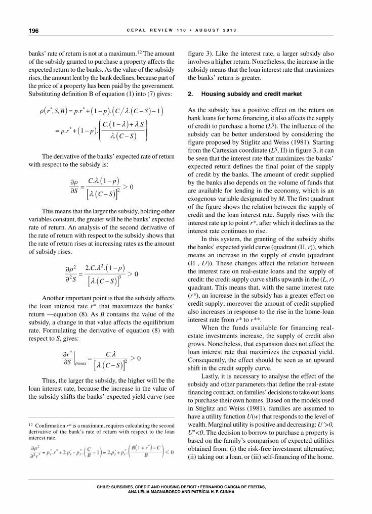
Thus, the larger the subsidy, the higher will be the loan interest rate, because the increase in the value of the subsidy shifts the banks’ expected yield curve (see
12 Confirmation r* is a maximum, requires calculating the second derivative of the bank’s rate of return with respect to the loan interest rate.
figure 3). Like the interest rate, a larger subsidy also involves a higher return. Nonetheless, the increase in the subsidy means that the loan interest rate that maximizes the banks’ return is greater.
2. Housing subsidy and credit market
As the subsidy has a positive effect on the return on bank loans for home financing, it also affects the supply of credit to purchase a home (LS). The influence of the subsidy can be better understood by considering the figure proposed by Stiglitz and Weiss (1981). Starting from the Cartesian coordinate (LS, Π) in figure 3, it can be seen that the interest rate that maximizes the banks’ expected return defines the final point of the supply of credit by the banks. The amount of credit supplied by the banks also depends on the volume of funds that are available for lending in the economy, which is an exogenous variable designated by M. The first quadrant of the figure shows the relation between the supply of credit and the loan interest rate. Supply rises with the interest rate up to point r*, after which it declines as the interest rate continues to rise.
In this system, the granting of the subsidy shifts the banks’ expected yield curve (quadrant (Π, r)), which means an increase in the supply of credit (quadrant (Π , Ls)). These changes affect the relation between the interest rate on real-estate loans and the supply of credit: the credit supply curve shifts upwards in the (L, r) quadrant. This means that, with the same interest rate (r*), an increase in the subsidy has a greater effect on credit supply; moreover the amount of credit supplied also increases in response to the rise in the home-loan interest rate from r* to r**.
When the funds available for financing real-estate investments increase, the supply of credit also grows. Nonetheless, that expansion does not affect the loan interest rate that maximizes the expected yield. Consequently, the effect should be seen as an upward shift in the credit supply curve.
Lastly, it is necessary to analyse the effect of the subsidy and other parameters that define the real-estate financing contract, on families’ decisions to take out loans to purchase their own homes. Based on the models used in Stiglitz and Weiss (1981), families are assumed to have a utility function U(w) that responds to the level of wealth. Marginal utility is positive and decreasing: U´>0, U''<0. The decision to borrow to purchase a property is based on the family’s comparison of expected utilities obtained from: (i) the risk-free investment alternative; (ii) taking out a loan, or (iii) self-financing of the home.

c e p a l r e v i e w 1 1 0 • a u g u s t 2 0 1 3
chile: subsidies, credit and housing deficit • fernando garcia de freitas, ana lélia Magnabosco and patrícia h. f. cunha
197
In the first case, the family does not purchase the property but rents their housing. All family resources are invested risk-free financial assets. The expected utility of alternative (i) is defined as the utility associated with the value of the family’s initial wealth (w0), capitalized by the rate of return on the safe investment (r), less the rental payment.
.U U w r R1a 0/ + −_` i j (9)
If the family obtains a home loan (situation (ii)), the expected utility corresponds to equation (10), namely the probability-weighted sum of the utilities in the case of payment or non-payment of the debt. When the debt is paid, the family’s utility corresponds to the value of initial wealth less the down-payment made to purchase their own home, capitalized by the market interest rate, having deducted the principal and debt service on the home loan, plus the value of the property. If the loan is defaulted, the utility corresponds to the value of wealth less the down-payment for the purchase of the home,
capitalized by the market interest rate, less the value of the property which reverts to the bank.
. . .
. .
U U w E r B r C p
U w E r C p
1 1
1 1
*b 0
0
/ − + − + + +
− + − −
_ _ _b_ _b _
i i i li i l i (10)
If the family chooses to self-finance their house purchase (situation (iii)), the expected utility corresponds to expression (11). That value is virtually the same as in equation (9), except that the value of the property multiplied by r is deducted, instead of the rent.
. . .U U w C r C U w r C r1 1c 0 0/ − + + = + −_ _b _`i i l i j (11)
A direct comparison of equations (9) and (11) leads to the relation that defines the choice between the safe investment or self-financing of the property. The expected utility of self-financing is greater than that of the safe investment when the rental R exceeds the value of the property multiplied by the interest rate on the safe investment (C.r). The latter is the amount of financial
FIgurE 3
effect of the subsidy on the supply of credit
L
LS
r* r** r LS L** L*
L*
L**
Π
Source: prepared by the authors on the basis of Ana Lelia Magnabosco, “A política de subsídios habitacionais e sua influência na dinâmica de investimento imobiliário e no déficit de moradias do Brasil e do Chile”, São Paulo, Catholic university of São Paulo, 2011.

c e p a l r e v i e w 1 1 0 • a u g u s t 2 0 1 3198
Chile: SubSidieS, Credit and houSing defiCit • fernando garCia de freitaS, AnA LéLiA MAgnAbosco And PAtríciA H. F. cunHA
income that will be forgone because the money was invested in the property.13
The analysis of the decision to take out a loan entails comparing the expected utility functions (10) and (11). For that purpose, equation (10) is divided into two parts: the first indicates the value obtained when the loan is paid (subindex 1); and the second the value in the case of default (subindex 2). The first part of equation (10) can be written as follows:
. . . .U U w r C r B S r B r1 1 1 *b1 0/ + − + + + − +_ _ _ _b i i i il
Comparing the argument of this function with that of equation (11) shows that the expected utility of self-financing could be either greater or less than the expected utility of the loan (in the case of payment). When the following expression is positive, the expected utility of the loan (in the case of payment) is less than the expected utility of self-financing:
. .B S r B r1 1 0* 2+ + − +_ _ _i i i
This is so because the value of the subsidy, capitalized by the interest rate on the safe investment, is greater (in absolute terms) than the amount of the debt multiplied the difference between the interest rate on the safe investment and the rate on the real-estate loan. If there is no subsidy, clearly Ub1 < Uc. As the value of the subsidy rises, the expected utility of the loan tends to be greater than the expected utility of self-financing. The same is true when the home-loan interest rate tends towards the safe-investment rate.
The second part of equation (10), related to subindex 2, can be written as follows :
. .U U w r C E r1 1b2 0/ + − − +_ _` i ij
A comparison of the argument of this function with that of equation (11) shows that the expected utility of self-financing can also be greater or less than the expected utility of the loan in the case of default. The condition is as follows: Uc is greater than Ub2 when C + E.(1+r) is greater than C.r. This happens when the interest-rate r is less than the ratio between (C + E) and (C – E), in other words, when the interest rate on the safe investment is
13 This relation shows that markets with a repressed rental value, or a very high interest rate on safe investments, discourage families from self-financing their properties.
not very high. For example, if E were equal to zero (0), the limiting two-period interest rate would be 100%. If there is an interest rate greater than 100% between the two periods,14 the expected utility of the loan tends to be greater than that of self-financing, as the value of the down-payment decreases.
In short, the expected utility of requesting a loan could be greater or less than the expected utility of self-financing. Nonetheless, loan contracts with a high subsidy and a small down-payment are known to increase the expected utility of choosing a loan. The same is true when the loan interest rate tends towards the rate on the safe investment. Moreover, low rental rates or high interest rates on the safe investment repress both self-financing and borrowing for the purchase of owner-occupied housing.
Family decisions are also affected by their level of wealth. In the case of very poor families with very little initial wealth w0, the amount of the down-payment (E) prevents them from entering the credit market. They are also unable to self-finance, because if their initial wealth is less than the value of the down-payment, it will also be less than the value of the property. Families in this situation put their sparse resources in the safe investment, and therefore rent their home.
In the case of families whose initial wealth is greater than the value of the property, it is assumed, on the basis of progressivity, that the homes they seek are not eligible for a state subsidy. In this case, as noted above, the utility of the loan is certainly less than that of self-financing if the debt is repaid (Ub1 < Uc). If the debt is not paid, for Ub2 to be less than Uc, the value of the property demanded by the family needs to be greater than half of the value of the debt, capitalized by the interest rate on the safe investment. If this is the case, the family will choose to self-finance their home. But even if the latter condition does not hold, it should be remembered that the probability of default declines as family wealth grows (equation (4)). For this reason, the decision to self-finance owner-occupied housing becomes more advantageous as the initial wealth of the families increases. Borrowing to purchase their own home is, therefore, an alternative typical of the middle-class.
14 This is a common level in real-estate financing plans. The two-period interest rate is the total value of interest paid in a financing operation divided by the value of the loan. In a financing plan with a constant instalment, for instance for a 30-year period and at an interest rate of 9% per year, the two-period interest rate would be 192%. If the annual interest rate were 6%, the two-period interest rate would be 118%.
c e p a l r e v i e w 1 1 0 • a u g u s t 2 0 1 3
chile: subsidies, credit and housing deficit • fernando garcia de freitas, ana lélia Magnabosco and patrícia h. f. cunha
199
A direct consequence of the above is that housing subsidies affect the demand for credit. When the subsidy value increases, the utility of loan financing rises and will exceed the utility of self-financing for some families. Moreover, the increase in the subsidy reduces the value of both the loan and the down-payment, and thus expands the set of families that apply for and are granted credit. Thus, the subsidies have a direct and positive effect on the demand for credit.
3. the housing subsidy and the dynamic of the real-estate market
The dynamic model of housing investment follows the formulation proposed by garcia and rebelo (2002), which is based on Muth (1960) and Tobin (1969). In this model, the economy consists of Nt families which grow at a constant rate of n. At time t, the demand for properties by the representative family, kt
d , depends on wealth (wt) and the rental value (Rt). The demand for properties is given by equation (12):
k f w g Rtd
t t= +_ _i i (12)
It is assumed that and and and ; in other words the variation in the demand for property with respect to wealth is positive and the variation with respect to the rental is negative. For convenience, it is assumed that g(Rt) is a linear function: g(Rt) = –β.Rt , β>0. In the short run, the supply of properties is fixed, and given by equation (13).
k k kts
t t0= = (13)
The rental value is determined by the equilibrium between demand and supply:
R
f w kt
t t
b=
−_ i
To analyse investor behaviour, the profitability of real-estate enterprises is defined. Following Tobin (1969), qt is defined as the ratio between the market price of the property (pmt) and the replacement cost of one unit of housing capital (ct). Assuming that the cost of construction is constant and equal to 1, qt is equal to the market price of the properties, which varies according to the profitability net of depreciation provided by the rental income on the asset.
q cpm
pmtt
tt= = (14)
The yield of the real-estate asset between two periods has three components: the capital gain qt , the rental income (Rt) and the physical depreciation (δ) of the asset, which is a proportion of the property value qt. The rate of return (rK) is defined as the ratio between the yield and the asset price.
.r q
q R qK
t
t t t/
d+ −o (15)
rearranging expression (15) gives:
.q r q RtK
t td= + −o _ i (16)
Substituting expressions (12) and (13) into equation (16), gives the dynamic equation qt:
.q r qf w k
tK
t
t td
b= + −
−o _ _i i
(17)
The model is completed by observing the variation in the amount of housing capital through time. By definition, the amount of capital in t is equal to the capital in t - 1, less capital depreciation in t, plus investment:
.K I Kt t td= −o . Dividing both sides of the equation by the number of families (Nt), and considering that
.k K N n kt t t t= −o o and i I Nt t t= , gives:
.k i n kt t td= − +o _ i (18)
Credit rationing is introduced into the general dynamic real-estate model through the families’ investment function (it). This function responds to the amount of credit offered by the banks and property prices, and is defined as the sum of the investment made by families classified in three classes according to their income level. Classes a and c encompass very wealthy and very poor families, respectively. Families of medium wealth belong to class b.
Very poor families, whose wealth is less than the down-payment on the property, do not have access to credit. In this case, their wealth is also less than the value of the property itself. Consequently, those families are not in a condition to self- finance and therefore rent their housing. real-estate investment serving that sector of
c e p a l r e v i e w 1 1 0 • a u g u s t 2 0 1 3200
Chile: SubSidieS, Credit and houSing defiCit • fernando garCia de freitaS, AnA LéLiA MAgnAbosco And PAtríciA H. F. cunHA
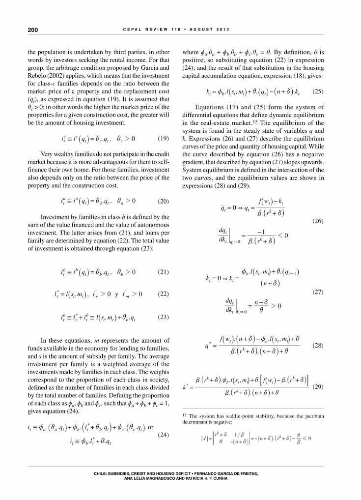
the population is undertaken by third parties, in other words by investors seeking the rental income. For that group, the arbitrage condition proposed by garcia and rebelo (2002) applies, which means that the investment for class-c families depends on the ratio between the market price of a property and the replacement cost (qt), as expressed in equation (19). It is assumed that θc > 0; in other words the higher the market price of the properties for a given construction cost, the greater will be the amount of housing investment.
. ,i i q q 0tc c
t c t c 2/ i i=_ i (19)
Very wealthy families do not participate in the credit market because it is more advantageous for them to self-finance their own home. For those families, investment also depends only on the ratio between the price of the property and the construction cost.
. ,i i q q 0ta a
t a t a 2/ i i=_ i (20)
Investment by families in class b is defined by the sum of the value financed and the value of autonomous investment. The latter arises from (21), and loans per family are determined by equation (22). The total value of investment is obtained through equation (23):
. ,i i q q 0tb b
t b t b 2/ i i=_ i (21)
mt y,l l s m l l0 0*t t s 2 2= ' ',_ i (22)
.i l i l s m q*tb
t tb
t t b t/ / i+ +,_ i (23)
In these equations, m represents the amount of funds available in the economy for lending to families, and s is the amount of subsidy per family. The average investment per family is a weighted average of the investments made by families in each class. The weights correspond to the proportion of each class in society, defined as the number of families in each class divided by the total number of families. Defining the proportion of each class as ɸa, ɸb and ɸc, such that ɸa + ɸb + ɸc = 1, gives equation (24).
or. . . . . . ,
. .
i q l q q
i l q
*
*
t a a t b t b t c c t
t b t t
/
/
z i z i z i
z i
+ + +
+
_ ` _i j i (24)
where ɸa.θa + ɸb.θb + ɸc.θc = θ. By definition, θ is positive; so substituting equation (22) in expression (24); and the result of that substitution in the housing capital accumulation equation, expression (18), gives:
t. . .k l s q n kt b t t tz i d= + − +,mo _ _ _i i i (25)
Equations (17) and (25) form the system of differential equations that define dynamic equilibrium in the real-estate market.15 The equilibrium of the system is found in the steady state of variables q and k. Expressions (26) and (27) describe the equilibrium curves of the price and quantity of housing capital. While the curve described by equation (26) has a negative gradient, that described by equation (27) slopes upwards. System equilibrium is defined in the intersection of the two curves, and the equilibrium values are shown in expressions (28) and (29).
.
.
q qr
f w k
dk
dq
r
0
10
t t k
t t
t
t
q k0t
&
1
b d
b d
= =+
−
=+
−=
o
o
__
_
ii
i
(26)
. .k k
n
l s q
dk
dq n
0
0
t t
b t t t
t
t
k
1
0t
&
2
d
z i
id
= =+
+
= +
-
=
, mo
o
__ _
ii i
(27)
. .
. .q
r n
f w n l s* t b t t
b d d i
d z i=
+ + +
+ − +k
, m
_ __ _ _
i ii i i
(28)
. .
. . . . .k
r n
r l s f w r*
b t t t
b d d i
b d z i b d=
+ + +
+ + − +
k
k k, m
_ __ _ _ _
i ii i i i: D
(29)
15 The system has saddle-point stability, because the jacobian determinant is negative:

c e p a l r e v i e w 1 1 0 • a u g u s t 2 0 1 3
chile: subsidies, credit and housing deficit • fernando garcia de freitas, ana lélia Magnabosco and patrícia h. f. cunha
201
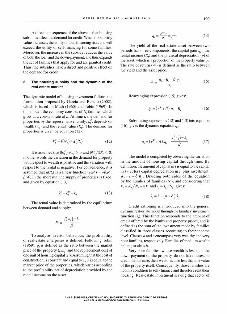
Lastly, the effects on housing-market equilibrium of changes in the system’s exogenous variables need to be evaluated, namely the amount of subsidy per family (st), the value of funds available for lending per family (mt), average family wealth (wt) and the rate of growth of the number of families (nt). An increase in the amount of subsidy per family reduces the value of the property and increases the amount of capital. Those effects, described by the partial derivatives set out below, correspond to a downward shift in the curve k 0t =o (see figure 4 (a)).16
and. .
.
. .
. . .
sq
n r
l
sk
n r
l r
0
0
'
'
k
b s
k
b sk
*
*
2
2
22
1
2
b d d i
z
b d d i
b z d
=+ + +
−
=+ + +
+
_ _
_ __
i i
i ii
If there is an increase in loanable funds in the economy, the price of the property will fall and the amount of capital should increase. This is because the curve k 0t =o also shifts downwards (see figure 4(b)). These effects are described through the partial derivatives:
16 In this model, the effects of the subsidy on the price of the property and the equilibrium amount of housing capital tend to be greater in societies with a relatively larger middle class.
and. .
.
. .
. . .
q
n r
l
n r
l r
m
mk
0
0
'
'
k
b m
k
b mk
*
*
2
2
22
1
2
b d d i
z
b d d i
b z d
=+ + +
−
=+ + +
+
_ _
_ __
i i
i ii
An increase in family wealth raises the market price of properties and increases the amount of housing capital. In this case, there is an upward shift in the curve qto = 0 (see figure 4(c)). That the effect is described through the partial derivatives of q* and k* with respect to wt . Faster population growth raises the market price of properties and reduces the amount of housing capital per family, as a result of an upward shift in the curve k 0t =o .
and. .
.
. .
.
q
n r
n f w
n r
f w
w
wk
0
0
'
k
t
k
t
*
*
2
2
22
2
2
b d d i
d
b d d i
i
=+ + +
+
=+ + +
'
_ _
_ _
_ __
i i
i i
i ii
and. .
. .
. .
nq
n r
k
nk
n r
k r
0
0
k
t
k
tk
*
*
2
2
22
2
2
b d d i
b d d i
b d
=+ + +
=+ + +
− +
_ _
_ __
i i
i ii
FIgurE 4
changes in the steady-state equilibrium
(a) (b)
Effect of and increasein subsidies per
family
Effect of an increasein loanable
funds
Effect of faster growthin the number
of families
Effect of an increasein family wealth
qt
q*
q1*
qt
q*
q1*
qt
q1*
q*
qt
q1*
q*
ktk1*k*
ktk1*k*
ktk1*k*
ktk*k1*
k̇t = 0
q̇t = 0
k̇t = 0
q̇t = 0
k̇t = 0
q̇t = 0
k̇t = 0
q̇t = 0

c e p a l r e v i e w 1 1 0 • a u g u s t 2 0 1 3202
Chile: SubSidieS, Credit and houSing defiCit • fernando garCia de freitaS, AnA LéLiA MAgnAbosco And PAtríciA H. F. cunHA
4. subsidies and housing deficit
garcia and rebelo (2002) proposed a formula for relating housing investment to the housing deficit, based on the hypothesis that there is an arbitrary level of income, yc, below which basic housing needs are not satisfied. In other words, below that level, the family is in a housing-deficit situation. This article adopts a similar approach, in which the critical variable is the amount of capital (kc).
The foregoing results show that family wealth and the amount of housing capital are positively related. Thus, for the critical level of capital kc, there is a critical wealth level wc. Families with a very low wealth level (wl) reach equilibrium with a small amount of steady-state capital; these are families in a deficit situation. Those that are not in deficit conditions have a higher level of wealth (wh). The steady-state price of properties (per m2) is also different for each class, which means that the property market is segmented.
The absolute and relative housing deficit is given by:
and.
.
.
D k dk d
k dk
k dk
i i i
i
i
k
k
0
0
0
c
c
r
r
r
= = 3__
_
ii
i
#
## (30)
where Di is the absolute housing deficit in a given region i; di is the relative deficit; and πi(k) is the distribution of the
amount of housing capital. The integral of the numerator shows the number of families with a capital reserve of up to the critical level, and that of the denominator indicates the total number of families. This reasoning is illustrated in figure 5.
FIgurE 5
Distribution of families by amount of housing capital and deficit
N
kkc
Subject to housing de�cit
Not subject to housing de�cit
πi(k)
π'i(k)
Source: prepared by the authors on the basis of Fernando garcia and André rebelo, “Déficit habitacional e desigualdade da renda familiar no Brasil”, Revista de Economia Aplicada, vol. 6, No. 3, São Paulo.
As shown in figure 5, the subsidies policy has the effect of redistributing the amount of capital from πi(k) to π'i(k), which expands the sector of the population
(c) (d)
Effect of and increasein subsidies per
family
Effect of an increasein loanable
funds
Effect of faster growthin the number
of families
Effect of an increasein family wealth
qt
q*
q1*
qt
q*
q1*
qt
q1*
q*
qt
q1*
q*
ktk1*k*
ktk1*k*
ktk1*k*
ktk*k1*
k̇t = 0
q̇t = 0
k̇t = 0
q̇t = 0
k̇t = 0
q̇t = 0
k̇t = 0
q̇t = 0
Source: prepared by the authors on the basis of Ana Lelia Magnabosco, “A política de subsídios habitacionais e sua influência na dinâmica de investimento imobiliário e no déficit de moradias do Brasil e do Chile”, São Paulo, Catholic university of São Paulo, 2011.
Figure 4 (concluded)

c e p a l r e v i e w 1 1 0 • a u g u s t 2 0 1 3
chile: subsidies, credit and housing deficit • fernando garcia de freitas, ana lélia Magnabosco and patrícia h. f. cunha
203
that is above the critical housing capital level, and thus reduces the absolute number of families living in a deficit situation. Similarly, an increase in investment funds (m) or family wealth (w) reduces the housing deficit in both
absolute and relative terms, whereas faster demographic growth increases it.
, , , , , , ,D f s w m n f f f f0 0 0 0i i i i i s w m n1 1 1 2= ' ' ' '_ i (31)
IV effect of the subsidy on housing credit
This section uses an econometric model to examine the determinants of credit in Chile and the role played by subsidies in that process. The empirical analysis is based on data from the 2009 casen survey, undertaken by the Ministry of Social Development (formerly the Ministry of Planning and Cooperation – mideplan). The survey interviewed 84,946 families. The monetary variables were standardized in dollars adjusted to purchasing power parity in Chile at 2009 prices.17
A logistic regression model was used to identify the factors that determine the probability of obtaining credit. Access to credit (c) is a variable with a binary distribution, which indicates whether the family obtained the property using credit (c=1) or not (c=0). The estimated function is described through equation (32):
P c X G x x
G X
1 … k k0 1 1
0
b b b
b b
= = + + +
= +
_ __
i ii (32)
where G(z) is a logistic function that takes values between zero (0) and one (1) for all real numbers z, such that:
exp
expG z
z
zz
1K=
+=_ _`
__i ij
ii 18
The set of variables that affect the probability of a family having access to credit (X) includes: its access to subsidy programmes; its monthly family income; the number of family members; the age of the head of the family; his or her level of schooling; the location
17 The conversion factor was taken from World Development Indicators (online), World Bank.18 This is the cumulative distribution function of a standard logistic random variable.
of the home in rural or urban zones; regional units, and a dummy time variable (representing the financing regime) to distinguish homes acquired after 1976, the year in which the Chilean housing financing system was reformed.
The regression results are reported in detail in table 3.19 The coefficients of income, access to subsidy, financing regime and schooling of the head of the household are all positive and significant; in other words as those variables increase, the probability of obtaining credit also rises. The coefficient on the subsidy variable is on the order of three, which means that if the family receives a subsidy, its chances of obtaining credit improve considerably. The financing regime variable displayed a positive and significant coefficient: after 1976, the chances of obtaining credit for own-home purchase are almost 20 percentage points higher than in the previous period. This reflects the effect of the policies promoted in that period, which restored the conditions of real-estate credit in Chile.
The empirical model described above corroborates the idea that access to the subsidy improves the chances of gaining access to credit. The subsidy thus supplements the income of poor families and reduces the banks’ credit risk, allowing both the demand for and the supply of credit to expand. Nonetheless, the model’s major shortcoming is the absence of other control variables for the supply of credit in the Chilean real-estate market. The casen survey that was analysed encompasses homes acquired between 1930 and 2009, in other words those purchased with and without credit under a very different macroeconomic conditions and credit regimes (see section II).
19 As the casen is a sample-based survey, each observation has a weight attributed to it by the sample selection process. The regression used the observations weighted by their respective sample weights.

c e p a l r e v i e w 1 1 0 • a u g u s t 2 0 1 3204
Chile: SubSidieS, Credit and houSing defiCit • fernando garCia de freitaS, AnA LéLiA MAgnAbosco And PAtríciA H. F. cunHA
As noted in the theoretical model, macroeconomic conditions affect the supply of funds for real-estate credit; and the value of the down-payment (related to prior saving) affects the relation between the size of the mortgage and the amount of the loan, with repercussions on the return to the banks and their willingness to lend. Owing to the restructuring of the credit system, reform of the pension system, and continuing expansion of banking services that occurred during the period under analysis, the supply of funds in the Chilean economy and prior family saving both grew considerably in those years. The proportion of families using credit to buy homes also increased. Figure 6 clearly shows the rising trend of that proportion and distinguishes three historical levels, which can be associated with the credit regimes described in section II of this article: up to 1959, between 1959 and 1976, and after 1976.
In this context, it is reasonable to ask whether the omission of those factors has a decisive effect on the estimation of the influence of access to the subsidy on access to credit. As there is no way of distinguishing
credit supply conditions between the individuals in the sample, they are assumed to vary very little through time. One way of capturing the influence of those conditions on the chances of access is to include dummy variables in the logistic regression to indicate the year in which the property was purchased. The set of dummy variables informs the conditions of credit supply, thereby balancing the model’s set of explanatory variables.20 The new calculations are shown in table 4.21
20 This reasoning implies that macroeconomic conditions and the aggregate volume of prior family saving in a given year affects the chances of obtaining credit for all families that acquired their homes in that year, in the same way and with the same intensity.21 The set of dummy variables that express the year of purchase is significant according to the maximum likelihood test (lr). The calculated value of the lr statistic is 87,600, way above the critical value for any conventional significance level. Accordingly, the null hypothesis that the coefficients on the dummy variables representing the year of home purchase are not significant, is rejected. The value of the estimated coefficients captures the rising trend of the chances of obtaining credit, as illustrated in figure 6.
TABLE 3
chile: logistic regression of access to credit
CoefficientStandard deviation
z P>|z|Confidence interval (95%)
Lower upper
Monthly income of the family (ln) 0.3442 0.00144 239.86 0.0000 0.3414 0.3471Access to the subsidy 2.8449 0.00311 915.50 0.0000 2.8389 2.8510Financing regime 0.1966 0.00365 53.91 0.0000 0.1894 0.2037
Number of persons -0.0538 0.00077 -69.50 0.0000 -0.0553 -0.0522Age of head of family -0.0016 0.00010 -15.74 0.0000 -0.0018 -0.0014Schooling of head of family 0.0965 0.00038 254.18 0.0000 0.0958 0.0973
urban area (0 or 1) 1.1454 0.00495 -231.24 0.0000 -1.1551 -1.1357regionI Tarapacá 0.6749 0.01654 40.80 0.0000 0.6424 0.7073II Antofagasta 0.2965 0.01640 18.08 0.0000 0.2643 0.3286III Atacama 0.9405 0.01819 51.71 0.0000 0.9049 0.9762IV Coquimbo 1.0538 0.01556 67.74 0.0000 1.0233 1.0843V Valparaíso 0.8854 0.01476 59.97 0.0000 0.8565 0.9144VI Libertador O’Higgins 0.9905 0.01546 64.08 0.0000 0.9602 1.0208VII Maule 0.5674 0.01523 37.25 0.0000 0.5376 0.5973VIII Bío Bío 0.7269 0.01470 49.44 0.0000 0.6981 0.7557IX La Araucanía 0.5393 0.01541 35.00 0.0000 0.5091 0.5695X Los Lagos 0.7141 0.01511 47.27 0.0000 0.6845 0.7437XI Aysén 0.4735 0.02293 20.65 0.0000 0.4285 0.5184XIII Metropolitan region 1.2471 0.01433 87.03 0.0000 1.2190 1.2752
Constant -6.4961 0.01945 -216.18 0.0000 -4.2434 -4.1671
Source: prepared by the authors on the basis of the 2009 National Socioeconomic Survey (casen).
Note: No. of weighted observations = 3,553,491. Degree of fit: -2 log of maximum likelihood = 3,340,059. Degree of fit (pseudo r2) = 32.04%.

c e p a l r e v i e w 1 1 0 • a u g u s t 2 0 1 3
chile: subsidies, credit and housing deficit • fernando garcia de freitas, ana lélia Magnabosco and patrícia h. f. cunha
205
FIgurE 6
chile: proportion of homes acquired with credit, 1949-2009(Percentages)
0
10
20
30
40
50
60
70
1949 1959 1969 1979 1989 1999 2009
Source: prepared by the authors on the basis of the 2009 National Socioeconomic Survey (casen).
TABLE 4
chile: logistic regression of access to credit, with dummy variables for year of purchase
CoefficientStandard deviation
z P>|z|Confidence interval (95%)
Lower upper
Monthly income of the family (ln) 0.3156 0.00143 221.20 0.0000 0.3128 0.3184Access to the subsidy 2.8449 0.00311 915.50 0.0000 2.8389 2.8510
Number of persons -0.0352 0.00077 -45.52 0.0000 -0.0367 -0.0337Age of head of family 0.0016 0.00011 15.10 0.0000 0.0014 0.0018Schooling of head of family 0.0968 0.00038 256.51 0.0000 0.0960 0.0975
urban area (0 or 1) 1.1993 0.00496 241.57 0.0000 1.1895 1.2090regionI Tarapacá 0.7667 0.01663 46.11 0.0000 0.7341 0.7992II Antofagasta 0.4507 0.01652 27.28 0.0000 0.4183 0.4831III Atacama 1.0398 0.01817 57.22 0.0000 1.0042 1.0755IV Coquimbo 1.1121 0.01576 70.54 0.0000 1.0812 1.1430V Valparaíso 0.9690 0.01498 64.67 0.0000 0.9396 0.9984VI Libertador O’Higgins 1.1386 0.01564 72.78 0.0000 1.1080 1.1693VII Maule 0.6774 0.01544 43.88 0.0000 0.6471 0.7077VIII Bío Bío 0.8243 0.01491 55.28 0.0000 0.7951 0.8535IX La Araucanía 0.6300 0.01559 40.41 0.0000 0.5994 0.6605X Los Lagos 0.8000 0.01530 52.29 0.0000 0.7700 0.8300XI Aysén 0.6129 0.02269 27.01 0.0000 0.5684 0.6574XIII Metropolitan region 1.3805 0.01455 94.85 0.0000 1.3520 1.4090
Constant -5.7599 0.26354 -21.86 0.0000 -6.2764 -5.2434
Source: prepared by the authors on the basis of the 2009 National Socioeconomic Survey (casen).
Note: No. of weighted observations = 3,553,491. Degree of fit: -2 log of maximum likelihood = 3,427,659.4. Degree of fit (pseudo r2) = 33.43%.

c e p a l r e v i e w 1 1 0 • a u g u s t 2 0 1 3206
Chile: SubSidieS, Credit and houSing defiCit • fernando garCia de freitaS, AnA LéLiA MAgnAbosco And PAtríciA H. F. cunHA
The results shown in table 4 reinforce those reported in table 3, because the coefficient that relates access to the subsidy to access to credit has the same sign and magnitude. The same can be said of the coefficients on the other explanatory variables, except for that relating the age of the head of family to access to credit. This coefficient changes sign, from negative to positive, thereby suggesting that the older the head of the family, the greater the chances of obtaining credit, which makes
more economic sense. The correction of the coefficient reflects the fact that there is a naturally positive correlation between the year of purchase of the home and the age of the head of the family, which, if not controlled for, biases the coefficient on that variable. Consequently, the macroeconomic and institutional conditions that affect the supply of credit help not only to explain the chances of obtaining credit, but also to correct the model’s calculations.
V subsidies, credit and housing deficit in chile
This section analyses the housing deficit in Chile. After defining the methodology used in this article to measure the deficit and analysing its recent trend, the section investigates the factors that are decisive for the housing deficit, highlighting the role of the subsidies and real-estate credit.
1. Housing deficit
The Chilean housing deficit can be measured in several different ways. Simian (2010) mentions the three main methodologies: that used by the Ministry of Housing and urban Affairs (minvu); the methodology used by the Chilean Chamber of Construction; and that used by the Libertad y Desarrollo think tank. These differ conceptually, and the numerical calculations vary considerably from one to another.
Arriagada (2005) analyses the methods used to measure the housing deficit in Latin American countries, and identifies two concepts that are present in nearly all methodologies: Homes made from precarious materials and squatter households, in which more than one family shares a home, are classified as housing-deficit situations; in other words there is a need for immediate relocation and an increase in the number of homes.
This article uses a methodology based on Szalachman (2000) to estimate the housing deficit in Chile. This methodology is less restrictive and brings together the elements that are common to most of studies in this field. While allowing for comparisons with other countries, this methodology does not use income criteria to select
deficit families, which makes it possible to use income in the explanatory models of the housing deficit. Box 1 sets out the concepts used to estimate the housing deficit in Chile, which is analysed in the dimensions “Precarious housing” and “Cohabitation”.22
Table 5 shows the trend in the number of families in the two dimensions of housing deficit between 1996 and 2009. Firstly, the number of families living in precarious housing dropped sharply from 148,000 in 1996 to 67,000 in 2009, representing a 5.9% decrease per year between 1996 and 2009. The downward trend seems to be related to the systematic increase in housing subsidies and credit in the decades of 1990 and 2000.
Over the 13-year period, the number of families sharing a home with another family grew by 2.2% per year. In addition to displaying a trend that differs from that of precariousness, this sector represents between 16% and 19% of all Chilean families. This means that, over those years, family cohabitation continued to increase until 2006, despite the growth of subsidies and credit for families.
22 The concept of precarious housing used in this article did not take account of conditions outside the home, such as the existence of sewerage services, access to water, garbage collection and urban infrastructure. Those characteristics were not included in the analysis because the investment to construct such networks and services is not a matter of individual decision or a decision by the real-estate credit market. These are public services for which installation and operation is subject to other types of credit constraint and other decision processes. Those issues, which are highly important for the housing and urban context, require different treatment to that used in this article.

c e p a l r e v i e w 1 1 0 • a u g u s t 2 0 1 3
chile: subsidies, credit and housing deficit • fernando garcia de freitas, ana lélia Magnabosco and patrícia h. f. cunha
207
According to Housing Minister Patricia Poblete Bennett,23 many Chilean families live with their relatives because they lack conditions to maintain a home of their own. Those families should not even be considered in the housing deficit, because the construction of a home would not resolve the problem. Data obtained by the 2009 casen confirm that phenomenon. Of the over 941,000 families living in the residency of other families, 577,000 (61.3%) cite economic reasons for cohabitation. On the other hand, about 20% of families in that situation cite
23 The opinions of Patricia Poblete Bennett, Minister of Housing and urban Affairs of Chile, in the administration of President Michelle Bachelet, were taken from Magnabosco (2011) – Annex 2.5.
motives of family tradition or preference for shared housing. The same survey notes that a minority (42.2%) of cohabiting families had plans to build their own home in the next few years.24
2. Factors determining the deficit
The empirical analysis developed in this section also uses the database of the 2009 casen survey. As in the analysis of the relation between credit and subsidy, the
24 The methodology used to calculate the housing deficit in Brazil, which was developed by the João Pinheiro Foundation, does not count families that do not intend to build a home of their own.
BOX 1
concepts used to estimate the housing deficit
Components Specification
Precariousness Families who live in homes included in at least one of the three following categories:
(i) Improvised housing Locations and properties not intended for residential use which serve as alternative housing (commercial properties, under bridges and viaducts, the shells of abandoned vehicles, boats, caves, among others)
(ii) rustic homes Those that do not have brick wall wooden walls
(iii) rented or donated homes Correspond to housing in rented or donated homes
Cohabitation Families who live in another family’s home
Source: prepared by the authors on the basis of Camilo Arriagada, “El déficit habitacional en Brasil y México y sus dos megaciudades globales: Estudio con los censos de 1990 y 2000”, Población y Desarrollo series, No. 62 (LC/L.2433-P), Santiago, Chile, Economic Commission for Latin America and the Caribbean (eclac), 2005. united Nations publication, Sales No. S.05.II.g.179.
TABLE 5
chile: number of families in a housing-deficit situation, 1996 to 2009
Year Precarious housing Family cohabitation Total families relative deficit (percentages)
Precarious housing Family cohabitation
1996 147 915 711 172 4 334 620 3.41 16.411998 164 615 745 667 4 522 690 3.64 16.492000 166 608 822 220 4 723 832 3.53 17.412003 116 835 898 422 5 028 826 2.32 17.872006 78 717 975 828 5 312 894 1.48 18.372009 66 859 941 377 5 626 867 1.19 16.73Variation (percentages)a -5.90 2.20 2.00 -2.22 0.32
Source: prepared by the authors on the basis of the National Socioeconomic Survey (casen) (various years).
a In the case of the relative deficit, this is measured as the percentage-point difference between 1996 and 2009.

c e p a l r e v i e w 1 1 0 • a u g u s t 2 0 1 3208
Chile: SubSidieS, Credit and houSing defiCit • fernando garCia de freitaS, AnA LéLiA MAgnAbosco And PAtríciA H. F. cunHA
family-income variable was standardized in dollars, adjusted for purchasing power parity in Chile, at 2009 prices.
The dependent variables of the logistic regression models used to identify the determinants of the deficit are membership of the group living in precarious housing (0 no; 1 yes), and membership of the group living in a situation of cohabitation (0 no; 1 yes). The estimated equations are specified in expression (32) of the previous section, and the distributions depend on the variables that indicate whether the families have access to the subsidy programmes and credit and, also, monthly family income. The set of control variables includes the number of family members, the age of the head of the family, his or her level of schooling, the location of the home in rural or urban zones, and regional units. Tables 6 and 7 report the results of the logistic regressions to determine the probability of being in a housing-deficit situation owing to precariousness and cohabitation.
The results shown in table 6 are highly significant. The coefficients on income, access to credit and access to the subsidy are negative. As family income rises, the likelihood of being subject to a housing deficit on the grounds of precariousness declines. Access to credit and the subsidy also considerably reduce the probability of a family living in precarious housing; as do the number of family members, and the age and schooling of family heads. The spatial variables indicate that housing deficit is less prevalent in urban areas and in the southern regions of the country. In contrast, the regions in which families are most likely to live in precarious housing are Antofagasta and Atacama.
The results reported in table 7 on the probability of belonging to the group of cohabiting families are even more significant. The coefficients on income and access to the subsidy are negative, which indicates that access to the subsidy and higher family income reduce the chances
TABLE 6
chile: logistic regression of membership of the group living in precarious housing
CoefficientStandard deviation
z P>|z|Confidence interval (95%)
Lower upper
Monthly income of the family (ln) -0.3553 0.00362 -98.03 0.0000 -0.3624 -0.3482Access to credit -2.2771 0.03476 -65.52 0.0000 -2.3453 -2.2090Access to the subsidy -1.5298 0.02546 -60.09 0.0000 -1.5797 -1.4799
Number of persons -0.4027 0.00271 -148.68 0.0000 -0.4080 -0.3973Age of head of family -0.0396 0.00028 -141.53 0.0000 -0.0402 -0.0391Schooling of head of family -0.1146 0.00111 -102.94 0.0000 -0.1168 -0.1124
urban area (0 or 1) -0.3799 0.01095 34.68 0.0000 0.3584 0.4013regionI Tarapacá 1.7048 0.30313 12.41 0.0000 3.1692 4.3574II Antofagasta 3.0099 0.30207 16.78 0.0000 4.4764 5.6605III Atacama 2.8765 0.30242 16.32 0.0000 4.3423 5.5278IV Coquimbo 2.1969 0.30213 14.08 0.0000 3.6633 4.8476V Valparaíso 1.9148 0.30190 13.16 0.0000 3.3816 4.5651VI Libertador O’Higgins 2.1299 0.30200 13.87 0.0000 3.5965 4.7804VII Maule 1.3610 0.30222 11.31 0.0000 2.8272 4.0119VIII Bío Bío 1.7982 0.30185 12.78 0.0000 3.2651 4.4483IX La Araucanía 1.4872 0.30218 11.73 0.0000 2.9534 4.1380X Los Lagos 1.5587 0.30203 11.98 0.0000 3.0253 4.2092XI Aysén -2.0585 0.32746 6.29 0.0000 1.4167 2.7003XIII Metropolitan region 2.2047 0.30170 14.13 0.0000 3.6719 4.8546
Constant 0.8941 0.30328 -6.34 0.0000 -2.5185 -1.3297
Source: prepared by the authors on the basis of the 2009 National Socioeconomic Survey (casen).
Note: No. of weighted observations = 5,431,713. Degree of fit: -2 log of maximum likelihood = 593,702. Degree of fit (pseudo r2) = 15.89%.

c e p a l r e v i e w 1 1 0 • a u g u s t 2 0 1 3
chile: subsidies, credit and housing deficit • fernando garcia de freitas, ana lélia Magnabosco and patrícia h. f. cunha
209
of belonging to the cohabiting group. Access to credit, in contrast, increases the likelihood that a family shares housing with another family. The number of people in the family and the level of schooling of family heads have a positive effect on that probability, indicating that cohabitation is more frequent among larger families whose head has a higher education level. The age of the head of the family has a negative coefficient, indicating that cohabitation is more frequent in families headed by young people. The spatial variables show that housing deficit is more frequent in urban areas and in the country’s most heavily populated regions: the Metropolitan region of Santiago and the Libertador Bdo. O’Higgins region.
Special attention should be paid to the positive coefficient relating access to credit to the likelihood of cohabitation, since those two variables could be reflecting other aspects of the behaviour of Chilean families that are not considered in the theoretical model
of the real-estate market developed in this article. Apart from cohabitation for reasons of preference and family tradition, some families have an economic strategy of sharing durable consumer goods and increasing the wealth of the family group.
The strategy of sharing consumer durables can be inferred from casen survey data. Ownership of this type of good is much more frequent among principal families than secondary families. In 2009, for example, 91.6% of principal families had a refrigerator, compared to just to 6.9% of secondary families. This indicates reliance on the refrigerator owned by the principal family. The strategy to increase the wealth of the family group is reflected in the number of secondary families that have their own property or are paying a mortgage (287,500, or 30.5% of cohabiting families). The homes of those families are mostly rented, which increases the income flow of the family group.
TABLE 7
chile: logistic regression of membership of the group living in conditions of cohabitation
CoefficientStandard deviation
z P>|z|Confidence interval (95%)
Lower upper
Monthly income of the family (ln) -0.9295 0.00180 -517.23 0.0000 -0.9330 -0.9259Access to credit 0.0751 0.00480 15.66 0.0000 0.0657 0.0845Access to the subsidy -0.0464 0.00480 -9.67 0.0000 -0.0558 -0.0370
Number of persons 0.6503 0.00096 680.00 0.0000 0.6484 0.6522Age of head of family -0.0732 0.00014 -527.73 0.0000 -0.0735 -0.0730Schooling of head of family 0.1121 0.00053 212.57 0.0000 0.1111 0.1131
urban area (0 or 1) 0.0954 0.00545 -17.53 0.0000 -0.1061 -0.0848regionI Tarapacá 0.5279 0.02090 2.14 0.0320 0.0039 0.0858II Antofagasta 0.7758 0.02052 14.26 0.0000 0.2525 0.3329III Atacama 0.2476 0.02291 -10.28 0.0000 -0.2804 -0.1906IV Coquimbo 0.4963 0.02053 0.64 0.5190 -0.0270 0.0535V Valparaíso 0.5857 0.01951 5.26 0.0000 0.0644 0.1408VI Libertador O’Higgins 0.8367 0.02011 17.59 0.0000 0.3142 0.3930VII Maule 0.4005 0.02019 -4.09 0.0000 -0.1222 -0.0430VIII Bío Bío 0.4868 0.01945 0.19 0.8490 -0.0344 0.0418IX La Araucanía -0.0545 0.02052 -26.20 0.0000 -0.5778 -0.4974X Los Lagos 0.4856 0.01988 0.13 0.9000 -0.0365 0.0415XI Aysén 0.4831 0.03284 -14.71 0.0000 -0.5474 -0.4187XIII Metropolitan region 0.8278 0.01905 18.10 0.0000 0.3074 0.3821
Constant 2.7273 0.02384 142.65 0.0000 3.3545 3.4480
Source: prepared by the authors on the basis of the 2009 National Socioeconomic Survey (casen).
Note: No. of weighted observations = 5,431,713. Degree of fit: -2 log of maximum likelihood = 2,675,684. Degree of fit (pseudo r2) = 40.85%.

c e p a l r e v i e w 1 1 0 • a u g u s t 2 0 1 3210
Chile: SubSidieS, Credit and houSing defiCit • fernando garCia de freitaS, AnA LéLiA MAgnAbosco And PAtríciA H. F. cunHA
This article has analysed housing policy in Chile, where far-reaching reforms were implemented in the housing finance system in the mid-1970s; and it highlights the strategy of combining credit with a subsidy in real-estate financing. That policy achieved positive results in combating the housing deficit, particularly in reducing the number of precarious homes, and it became a reference in this field for Latin America. Beyond individual government programmes, Chilean housing policy has gained the status of a state policy, maintained across several government administrations with different ideological tendencies.
Based on the financing system in Chile, in which the property is purchased using resources based on prior saving, credit and subsidy, a theoretical model was developed to analyse the influence of the housing subsidies policy on the credit market and on the real-estate market. The granting of subsidies for home purchase increases the return on bank loans and expands the supply of credit. The subsidy also boosts the demand for loans. An increase in subsidies and the expansion of the supply of credit change the equilibrium in the real-estate market, resulting in an increase in housing capital per family and a reduction in property prices, with repercussions on the housing deficit.
Those theoretical relations guided the econometric analyses undertaken in the following sections, the results of which results for Chile corroborate the theoretical proposals formulated in the article. The most important new theoretical results were not refuted by the data: (i) access to the subsidy has a decisive influence on the granting of credit, directly increasing a family’s chances of obtaining credit; and (ii) an increase in the amount of the subsidy reduces the number of families with housing capital below the critical level, in other words those living in housing-deficit situations.
The econometric results also help in interpreting the trend of the housing deficit in Chile between 1996 and 2009. New subsidies were granted year by year, and
the percentage of families assisted by this policy grew. Whereas in 1996, 20.9% of Chilean families had received some type of housing subsidy, by 2009 the proportion had risen to 28.2%. Credit also flowed liberally: the proportion of families with access to real-estate credit rose from 22.3% in 1996 to 31.0% in 2009. The average income of Chilean families grew from uS$1,600, in purchasing- power-parity terms, to uS$ 2,100 —equivalent to 27% growth in the period analysed.
That trend of credit and subsidies, together with the growth of family incomes, led to a gradual reduction in the deficit caused by precariousness, as predicted by the theoretical model and in the econometric analysis. The trend of those variables also explains the relative persistence of families living in situations of cohabitation. In the reference period, the proportion of families with access to credit grew, and Chile became more urbanized,25 factors that ended up increasing the frequency of cohabitation. Increased access to the subsidy, higher average family income, and the lower average age of heads of family apparently prevented cohabitation from increasing by even more.26
The results show that Chile’s housing subsidies policy has considerable effects on the deficit, reducing precariousness and reorganizing its dimensions, with a relative increase in family cohabitation. The tests undertaken add to knowledge of the effects of housing policy, which is useful not only for analysing the Chilean real-estate market, but also for research in other Latin American countries, such as Brazil and Mexico, which adopted policies similar to those of Chile in the decade of 2000.
25 In absolute terms, between 1996 and 2009, 1,167,000 new families were formed in urban areas in Chile compared to just 83,000 new families in rural areas. The proportion of families living in urban areas rose from 85.7% to 87.4% in the same period.26 The average age of heads of family rose from 45.6 years in 1996 to 49.3 in 2009.
VI Final thoughts

c e p a l r e v i e w 1 1 0 • a u g u s t 2 0 1 3
chile: subsidies, credit and housing deficit • fernando garcia de freitas, ana lélia Magnabosco and patrícia h. f. cunha
211
Arriagada, Camilo (2005), “El déficit habitacional en Brasil y México y sus dos megaciudades globales: Estudio con los censos de 1990 y 2000”, Población y Desarrollo series, No. 62 (LC/L.2433-P), Santiago, Chile, Economic Commission for Latin America and the Caribbean (eclac). united Nations publication, Sales No. S.05.II.g.179.
Brain, Isabel, gonzalo Cubillos and Francisco Sabatini (2007), “Integración social urbana en la nueva política habitacional”, Temas de la Agenda Pública, year 2, No. 7, Santiago, Chile, Catholic university of Chile.
Castillo, Maria José and rodrigo Hidalgo (2007), “1906/2006. Cien años de política de vivienda en Chile”, Arquitectura series, No. 1, Santiago, Chile, Ediciones unab.
Domínguez Vial, Vicente and María de la Luz Nieto de los ríos (1993), “Ahorro previo y subsidios para la adquisición de viviendas”, Políticas de financiamiento habitacional en Chile, Santiago, Chile, Social Security research Corporation (ciedess).
Fundação João Pinheiro (2009), Déficit habitacional no Brasil em 2007, Belo Horizonte.
garcia, Fernando and André rebelo (2002), “Déficit habitacional e desigualdade da renda familiar no Brasil”, Revista de Economia Aplicada, vol. 6, No. 3, São Paulo.
Magnabosco, Ana Lélia (2011), “A política de subsídios habitacionais e sua influência na dinâmica de investimento imobiliário e no déficit de moradias do Brasil e do Chile”, São Paulo, Catholic university of Chile.
mideplan (Ministry of Planning and Cooperation) (1996-2009), “Encuesta de Caracterización Socioeconómica Nacional”, Santiago, Chile.
minvu (Ministry of Housing and urban Affairs) (2007), Un siglo de políticas de vivienda y barrio, Santiago, Chile.
Morandé, Eugenio (1993), “El mercado inmobiliario habitacional”, Políticas de financiamiento habitacional en Chile, Santiago, Chile, Social Security research Corporation (ciedess).
Muth, richard (1960), “The demand for non-farming housing”, The Demand for Durable Goods, Arnold C. Harberger, Chicago, The university of Chicago Press.
Simian, José Miguel (2010), “Logros y desafíos de la política habitacional en Chile”, Estudios Públicos, No. 117, Santiago, Chile, Centre for Public Studies.
Stiglitz, Joseph and Andrew Weiss (1981), “Credit rationing in markets with imperfect information”, American Economic Review, vol. 71, No. 3, Nashville, Tennessee, American Economic Association.
Szalachman, raquel (2000), “Perfil de déficit y políticas de vivienda de interés social: Situación de algunos países de la región en los noventa”, Financiamiento del Desarrollo series, No. 103 (LC/L.1417-P), Santiago, Chile, Economic Commission for Latin America and the Caribbean (eclac), September. united Nations publication, Sales No. S.00.II.g.89.
Tobin, James (1969), “A general equilibrium approach to monetary theory”, Journal of Money, Credit and Banking, vol. 1, No. 1, Ohio, Ohio State university Press.
Bibliography