1

Child Labor and the Labor Supply of Other Household Members

Evidence from 1920 America

Marco Manacorda

CEP & STICERD, LSE

March 2003

I study the effect of child labor on the labor supply of different household members using 1920 US Census data. In order to identify a source of exogenous variation in child labor I use state child labor laws. First, I find a strong effect of child labor laws on labor market participation of individual children. Second, I find that a rise in average children labor force participation at the household level is associated with no variation in parents’ labor supply. However, as the proportion of working children by household rises, the probability that each individual child works falls while the probability that he attends school rises. This suggests that the returns from child labor are redistributed to children in the household rather than to parents, consistently with a model of child labor with altruistic parents. I am grateful to the Nuffield Foundation for the financial support provided under the New Career Development Scheme and to Jan Eeckhout, Maia Guell, Alan Manning, Steve Pischke and seminar participant at the LSE for comments and suggestions on a previus draft. I am also indebted to Adriana Lleras-Muney for making her data on child labor and compulsory schooling laws available and for clarifying some details of these laws. Address for correspondence: Center for Economic Performance, London School of Economics, Houghton Street, WC2 2AE, London, GB. m.manacorda@lse.ac.uk.

2

Introduction

In this paper I investigate the effect of child labor laws in 1920’s America and I explore the effect of a

rise in children’s labor force participation on other household members’ labor supply. I show how one

can use the labor supply responses of different household members as average children labor market

participation by household varies to infer the degree of parental altruism.

The assumption that parents are altruistic with respect to their children goes mainly

unchallenged in the theoretical literature (Becker, 1981), including the more recent literature on child

labor (e.g. Basu and Van 1998, Baland and Robinson 2000). However, the empirical evidence on

parents' altruism is mixed. Altonji et al. (1997) for example find only a modest degree of parental inter-

vivos altruism in contemporary and Parson and Goldin (1989), in a paper that is similar in spirit to the

present one, tend to reject parental altruism. The question is crucial because parental selfishness might

be at the root of individuals’ poor capital accumulation of human capital and policy intervention (in the

form of child labor laws for example) might be desirable if parents’ selfishness is associated to some

inefficiently low levels of education.

1920 America is a good testing ground for this analysis. This was a period of tremendous

transformation of the American economy (Goldin 1996; Goldin and Katz 1996, 1998) and while

educational attainment was raising very rapidly (Goldin, 1998, 1999a, 1999b; Goldin and Katz, 1999),

school attendance was not universal, especially in rural areas and a non negligible proportion of

children were involved in some form of work. By 1920, most US states had some child labor law but

still one million children between the ages of 10 and 15 were involved in some form of gainful

employment. While there is evidence that prior to then child labor laws had little effect (Sanderson,

1974; Moehling 1999), there is some consensus that by the early 1900s child labor laws had a

significant effect on children’s participation (Margo and Finegan, 1996; Acemoglu and Angrist 2000;

3

Lleras-Muney, 2001) so one can use child labor laws as a source of variation in children’s labor supply

that is arguably exogenous to the labor supply choices of other household members.

The structure of the paper is as follows. In Section 1 I present some basic evidence on the effect

of child labor laws on child labor force participation. Section 2 introduces a simple theoretical model of

household labor supply with child labor. I show how one can infer the degree of parental altruism by

looking at variations in household labor supply induced by (exogenous) changes in child labor. Section

3 examines carefully the patterns of labor force participation in 1920 America and presents the

regression results. Section 4 presents a variety of robustness checks and Section 5 concludes.

1. Labor markets, child labor and child labor laws in 1920 America

1.1 The background

The first decades of last century saw a massive transformation of the economy and the American

society (Goldin 1996; Goldin and Katz 1996, 1998). This was the period when automobiles, office

equipment, commercial radio and electrical household appliances entered the life of ordinary

Americans. Manufacturing, by far the most important sector of the economy, was undergoing profound

changes: the availability of new technologies and in particular of purchased electrical horsepower

prompted the passage from the traditional factory (assembly lines) to continuous and batch production

processes. This change in production technology was associated to a tremendous rise in the demand for

skilled labor.1 Changes in the labor market took place not only on the demand side but also on the

supply side. Immigration (especially of unskilled workers) boomed in the first decades of the century

1 This change contrasted with the first transformation of the American manufacturing sector (from the artisan shop to the factory) that took place during the 19th century and that brought about a rise in the demand for unskilled workers. Goldin and Sokoloff (1982) examine the rise and fall of child (and female) employment in manufacturing during the first half of the 19th century. They argue that employment of children in manufacturing peaked somewhere in the first half of that century (between the late 1830s and the early 1840s) and they track down this movement to a rise in demand for unskilled labor linked to general technical progress and to the increase in the share of manufacturing over total output. For a fascinating analysis of child labor in 19th century America see also Willoughby (1890).

4

until the onset of the World War I. Arguably as a partial consequence of the shift in the demand for

skills, the decades from 1910 to 1930 saw an unprecedented rise in high school attendance and

graduation of young Americans.2

The high school movement was the greatest transformation of American education (Goldin

1998, 1999a). New schools were built, school districts were consolidated and curricula were changed to

meet the needs of a middle class increasingly willing to enter the labor market after completion of high

school rather than continuing to college. The interplay between the demand for skills and the supply of

skills was crucial in shaping the outcomes in the labor market. (Goldin, 1999b; Goldin and Katz, 1999)

What evidence there exists, it suggests that skill premiums were high in the early 1910s and tended to

fall up to at least 1920. 3 High returns to education prompted an increased demand for schooling, which

in turn lowered returns and fostered further economic progress. 4 After 1920, high school graduation

and enrollment rose dramatically but returns stayed roughly constant up to 1940.

The tremendous rise in school attainment was associated with a fall in the employment of

children especially in manufacturing. Although there is some disagreement as to when exactly child

labor reversed its trend, certainly the decade between 1910 and 1920 was one of rapidly decreasing

labor force participation of children. Still, in 1920 around one million children aged 10 to 15

(approximately equal to 8.5% of the population in that age group) were involved in gainful occupations

according to the Census (down from about two million in the 1910 Census).5

2 There are pronounced differences across regions in the impetus of the high school movement. Expansion was particularly rapid in the non-south. By contrast, the movement towards the abolition of child labor was largely opposed by Southern capitalists who still employed cheap labor in agriculture well into the beginning of the 20th century. A separate issue regards blacks who were concentrated in the South. Almost the totality of black children attended segregated schools (Boozer et al., 1992) and the quality of their education was much lower than the one of whites (Card and Krueger, 1992). 3 Goldin and Katz (2000) based on data from Iowa estimate that the return to an additional year of high school for young male workers was about 12% in 1915. 4 Differentials fell somewhat during World War I, a likely effect of the rise in the demand for unskilled labor in the war period. 5 Notice however after world war the US entered into a recession with unemployment rising to a level estimated between 8.7% and 11.7%. Also, data from 1910 are not strictly comparable to the ones from the 1920 census since the former was conducted in April while the latter in January (a period in which agriculture is at a standstill).

5

There is some dispute in the literature as to whether child labor and compulsory schooling

legislation contributed to the falling trend in child labor force participation or whether legislation only

embodied ex-post the changes that had occurred in the labor market. A view that is generally held is

that legislation followed suit the great transformation of the American economy: the fall in the relative

importance of agriculture, the transformation of manufacturing with the associated rise in the demand

for skills, the rise in the supply of unskilled labor brought about by immigration, the secular increase in

standards of living and real wages, the increased availability of educational opportunities.6 7 Certainly,

however, the first two decades of the century saw the rise of a strong movement advocating more

stringent child labor legislation (Trattner, 1970). Although originally prompted by few social reformers

and philanthropists, the movement against child labor soon encountered the consensus of the middle

class. Civic participation was at its highest over the century,8 and the middle class, helped by

widespread propaganda, started to recognize the benefits of schooling and the ‘evils’ of child labor.

The decade between 1910 and 1920 is probably the one where the most progress was made in terms of

child labor legislation. Although later declared unconstitutional by the Supreme Court, two Federal

laws were passed in 1916 and 1919 that greatly limited the employment of children under age 14 and

restricted employment in several industries and occupations.9 The experience of the 1910s contrasted

6 Goldin (1998) argues though that secondary schooling was facilitated by a rich agricultural sector (which increased the base for taxation) and hindered by a large manufacturing sector (that created desirable employment opportunities for youth). 7 Sanderson (1974) concludes that it is unlikely that child labor legislation was a major force behind the fall in child labor. Landes and Solmon (1972) based on data for the end of 19th century argue that the passage of child labor legislation and compulsory schooling laws was largely endogenous to the initial level if schooling in the state. This view is also reported in many of Claudia Goldin’s papers quoted above. The existing evidence suggests that child labor and compulsory schooling legislation had little impact on participation of young Americans in the labor market up to 1920. Moehling (1999) finds little effect of child (manufacturing) labor laws on child work in turn of the century America. Her analysis though stops in 1910 and indeed she finds stronger effects for the decade after the turn of the century than for the period preceding it. Margo and Finegan (1996) though find a strong effect of compulsory schooling laws when used in conjunction with child labor laws on school attendance of 14-years old in 1900 America. 8 Putnam (2000) reports that civic participation was higher in the first decades of the last century than in any other period after that. 9 Both laws prohibited employment of children under fourteen in mills, canneries, workshops or factories, employment of children under sixteen in mines or quarries (Fuller, 1922).

6

with the experience of the previous decades: in late 19th century America child labor legislation was

uniform across states and poorly enforced.

1.2 Basic evidence

If there was a period when child labor legislation was potentially able to have an effect was indeed in

1920 America. By then all states had compulsory schooling laws and child labor legislation (in various

forms). Enforcement was stricter than ever before, possibly also a reflection of the change in people’s

attitudes and the increased pressure by the Federal Government.10 In order to investigate the effect of

child labor laws on children labor force participation, I integrate the data from the 1920 US census with

data on state child labor laws. The 1920 Census provides detailed information on the usual occupation

and industry of employment of individuals aged 10 or more.11 One drawback of the data however is

that no information on either work intensity (hours, days, weeks or months of work) or wages and

earnings is collected. Child labor laws refer to the minimum age at which a child can obtain a work

permit.12 13 14

Before presenting the basic evidence, it is worth speculating on the likely effects of child labor

laws on child labor. In the absence of a minimum working age, child labor force participation is likely

to grow with age. First, productivity (and hence the wage) grows with age. Second, parents might value

their children's leisure less as they grow up. Both these two effects make child labor less likely at early

10 What evidence there exists, it clearly suggests that child labor legislation had (probably more than compulsory schooling laws) a significant effect on school attainment of individuals born from 1914 onwards (see Section 3). 11 The concept of unemployment did not exist at that time. Individuals were classified according as to whether they had a gainful occupation or not. 12 Census data come from IPUMS (www.ipums.org). Data from child labor laws are the ones collected by Adriana Leeras-Muney and are available on her website (http://www.princeton.edu/~alleras/papers.htm). States had different provisions against child labor: the legislation set minimum working ages, prohibited employment in some occupations, set restrictions on working hours or specified educational requirements for employment. In this paper I only use data on minimum working age. As a general rule, there where different minimum ages were set for different types of child labor, the minimum of these ages in each state has been reported (personal communication to Adriana Lleras-Muney). 13 Work permits were generally administer and granted by schools (Angrist and Krueger, 1991). 14 My sample only refers to the 48 mainland states with the exclusion of the District of Columbia.

7

ages. When child labor laws exist, and assuming compliance, one would expect children below legal

working age not to work and one would expect a sharp rise in participation as a child turns minimum

working age. If job search is costly, and in the absence of other effects, one would expect child labor to

converge gradually towards the desired level (i.e. the one which would have prevailed in the absence of

child labor laws). Notice however that a second effect might be at work. If children are not allowed to

work at early ages, they (their parents) might make up for missed earnings in early years of life by

working (making them work) more as they turn legal working age. The hypothesis that child labor laws

induce individuals to inter-temporally substitute their labor supply introduces a further degree of

steepness in the employment age profile of children. Labor force participation in states affected by

child labor laws can potentially overshoot participation in states unaffected. Eventually, employment

rates will converge to their desired level. If child labor laws are not systematically related to the desired

level of labor force participation, employment among prime age individuals should be the same across

states.

In order to motivate this paper, in Figure 1 I report employment rates by age for individuals

aged 10-18 in seven groups of states, which I have classified based on their minimum working age.15

For each group of states the vertical line indicates the maximum age at which work is not permitted

(i.e. minimum working age minus one). In some states minimum working age is less than 10 and so no

vertical line is reported since this is to the left of 10. In principle everybody to the right of that vertical

line is allowed to work. The data are remarkably consistent with the predictions of the model. First,

children aged less than minimum working age virtually do not do any work. For example, the

employment rate in states with minimum working age of 14 stays flat until age 13 while in states with

15 Here employment includes both market work and work in the household enterprise. See below for a further discussion on these different types of work.

8

minimum working age of 7 or 8 it tends to increase roughly monotonically with age.16 Second,

participation starts to increase just after children turn minimum working age. While for example labor

force participation of children living in states with minimum working age equal 13 tends to grow

smoothly from age 13 onwards, for children living in states with minimum working age equal 14

participation increases only after this age. However, there is no discrete jump in employment: entry

into work takes place gradually and participation tends to grow more rapidly in the states with higher

minimum working age. There is evidence that these states tend to catch up in terms of youth labor force

participation with states where minimum working age is lower, and even to outperform them.

Eventually participation in different states converges to a similar level. In Figure A1 in the appendix I

report participation for individuals aged 10-30 in two groups of states which account for almost 90% of

the whole sample: those with minimum working age equal 12 and those with minimum working age

equal 14. It is remarkable how labor force participation of children in states with higher legal working

age rises rapidly from age 14 onwards, overshoots participation in states with lower legal working age

and then decelerates. By age 25 participation tends to be similar across states with different child labor

laws.17

In order to capture the effect of child labor laws on child labor force participation, I have fit a

statistical model to the data. Essentially I have estimated a linear spline in age with a kink at the age

just below minimum working age. The details of this model are presented in Section 3 where I discuss

my regression results. In Figure 2 I have superimposed this estimated curve to the actual series of labor

force participation. For now it is interesting to notice that this model predicts remarkably well the

actual employment series.

16 Notice however that there are pronounced differences in the number of children living in each of these different groups of states so some caution should be used in making these comparisons. See Section 3 for the distribution of children by legal working age.

9

The basic evidence in Figures 1 and 2 suggests that child labor laws had a discernible impact on

labor force participation. One can interpret this evidence as a suggestion that in the absence of child

labor laws different states would have experienced similar trends in children employment. This is

essentially one of the approaches I use in this paper to identify the effect of children's labor force

participation on household labor supply. Another possible but not necessarily mutually exclusive

interpretation of the data in Figures 1 and 2 is that in the absence of child labor laws, child labor would

have grown smoothly with age in each group of states. One can think of the discontinuity in the age

profiles that is apparent in Figures 1 and 2 to be the product of child labor laws and attempt to use this

discontinuity as a source of variation in child labor. This is the second approach I use in this paper to

identify arguably exogenous variations in child labor.

One last caveat of this analysis regards the possible underreporting of child labor in those states

where this was banned. In this case the evidence in Figure 1 has no behavioral content since it only

suggests that households did not report the labor of the children below legal working age. Possibly the

evidence in Figure A1 speaks against this alternative hypothesis. The observation that individuals tend

to work more in later years of life the higher legal working age is hard to reconcile with underreporting,

unless one believes that reporting errors are corrected only gradually over time and even push

individuals to over-report their participation at later stages of life. However this evidence is far from

conclusive and I try to add more evidence in this direction later on in the paper when I present my

regression results.

17 Some caution is needed in interpreting this data, since that individuals belonging to earlier cohorts might have been exposed to different child labor laws.

10

2. A stylized model of household labor supply with child labor

Before turning to analyzing empirically the effect of child labor on the labor supply of other household

members, in this section I present a simple model of household labor supply. I show that, unless parents

are altruistic, a rise in child labor should be associated to a fall in parents’ labor supply.18 19

To fix ideas, consider a household made by two individuals. For now assume that the two

individuals are a father and a child. Either individual can work or stay idle.20 The decision as to

whether each individual works is taken by the parent. In order to conform to the existing literature on

child labor, I use the same household labor supply model as in Basu and Van (1998). Differently from

Basu and Van (1998), though, I assume that some utility accrues to the household from consumption of

the parent’s leisure. Since in their model parents are altruistic, they are always at the corner (i.e. they

work irrespective of their own and their children's wage). Here instead parents might well be at the

interior solution or even be inactive. Their choice as to whether to work or not will depend not only on

their own market wage relative to their children's but also on the degree of their altruism.

Assume that parents maximize the following Stone-Geary utility function

(1) U(c,e1,e2)=(c-s)[(1-e1) 1-α(1-e2)α] c>=s

U(c,e1,e2)=(c-s) c<s

s.t. c=w1e1+w2e2

where c>=0 is household consumption that is a public good, 0<=e<=1 is effort (with 1 being the

endowment), s>=0 is the level of necessary consumption (net of any unearned income), w is the wage

18 And assuming that leisure of different household members are substitutes in the household utility function. 19 Obviously parents must be altruistic to some extent otherwise it is likely that children would not attend school. The issue here is whether they are fully altruistic i.e. whether to one extent they exploit their children. 20 The model can be easily rephrased so that the time children spend in non productive activities (leisure) is spent in school. If parents do not draw any direct utility from their children schooling (because of parents' mortality of because of the non-enforceability of contracts stipulating that part of the returns from children education will accrue to parents as children enter the labor market) then the conclusions of the model are unchanged. Indeed the evidence in Section 3 suggests that the large majority of non-working children were attending school.

11

rate and the subscripts 1 and 2 denote respectively the parent and the child.21 The utility function in (1)

states that the parent maximizes a combination of consumption and household leisure with α being the

weight that the parent attaches to his children’s leisure relative to his own. The budget constraint

simply states that consumption must me financed by either the parent's earnings or the child's or both.

Basu and Van’s (1998) model is a special case of (1) where α=1, i.e. the parent is fully altruistic. The

way the model is written implies that for consumption below the subsistence level both household

members will work. The parent maximizes the utility in (1) subject to the budget constraint. Three

outcomes are possible in equilibrium: either both individuals work or only one of them does.

1. e1>0, e2=0 if w2< α(w1 -s)/(2−α) (2) 2. e1=0, e2>0 if w2>(1+α)w1/(1−α)+s

3. e1>0, e2>0 if α (w1 -s)/(2-α)<w2<(1+α)w1/(1-α)+s

The equilibrium for this model in the w10w2 space (i.e. conditional on s and α) is depicted in Figure 3.

For very low wages both the parent and the child work: this is to guarantee some subsistence

consumption. For very low levels of the child's (father's) wage the father (child) will work irrespective

of his wage. If the wage of the child (father) grows sufficiently, the child (father) will invariably work

and the father (child) will eventually stop working. There are two effects at work: an income and a

substitution effect. On the one hand a rise in the child's wage tends to increase household income and to

reduce the father's labor supply. In addition, because the child and the parent leisure are substitutes in

the utility function (1), the substitution effect acts in the same direction. A rise in the child’s wage

21 While in Basu and Van (1998) c and s are respectively per-capita levels of consumption and subsistence consumption, in my notation these are household-level variables.

12

makes the child's leisure more expensive and the household substitutes away from the more expensive

input (the child’s leisure) towards the cheaper one (the father’s leisure).22

A way of thinking about child labor laws is they act in setting the market wage of children

below legal working age to zero.23 So one can use the diagram in Figure 3 to predict the effect of child

labor laws on the labor force participation of other household members. Conditional on the parent’s

wage (w1) (as well as the level of subsistence consumption (s) and preferences (α)), a rise in the child's

wage from zero to a positive number (i.e. the fact that the child turns minimum working age) has a non-

negative effect on the child labor force participation (from zero to a positive number). One can see this

by moving from any point on the horizontal axis (where child labor force participation is zero) to a

point above it. Either the child remains inactive (if the parent’s wage is sufficiently high or the parent is

sufficiently altruistic) or he starts working. Similarly, a rise in the child’s wage has a non-positive

effect on the participation of the father. The parent eventually withdraws from the labor market as his

child's wage rises. Again this effect depends on the degree of parental altruism.24

In the extreme case in which the parent is fully altruistic (α=1), the father will work irrespective

of the child’s wage (e1>0). In equilibrium the child might still work even if the parent is altruistic:

(3) e2>0 if w2>w1-s

I have depicted the extreme case in which parents are completely altruistic in Figure 4. The child will

work if either the parent’s earnings do not allow the household to reach a subsistence level of

22 In practice, it is hard to know a priori whether the child and the parent’s leisure are substitutes or complements in the utility function and in theory the overall effect of a rise in the child's wage is therefore a priori ambiguous. In my empirical estimates below I impose no restriction on these patterns of substitution. 23 This is the approach used, among others, by Deaton and Muellbauer (1980) in the context of commodity demand with rationing. One can derive a shadow price that is the price of leisure under which unconstrained households would chose zero working hours for children. Clearly a wage level that satisfies this property is a wage equal zero. For an analysis of household labor supply with rationing (i.e. involuntary unemployment) see Ashenfelter (1980). 24 If child labor legislation is only partly enforced (i.e. there is some non compliance), one can still use this framework to understand the effect of a child turning legal working age. In this case, turning legal working age is still associated with a rise in the child’ wage (although starting from a positive number rather than zero) and one can see that the main conclusions of the discussion above remain unchanged.

13

consumption (w1<s) or the disutility from the child’s work is lower that the marginal utility of an

additional unit of consumption. In this case, a rise in the child’s wage from zero to a positive number

(conditional on w2) has no effect on the parent’s participation, while it tends to have a non-negative

effect on the child's participation.

The discussion so far suggests that if the parent is altruistic (α=1), and conditional on his wage

(plus preferences and subsistence consumption), one should not expect any correlation between the

parent and the child's labor force participation as the latter increases exogenously because of a rise in

the wage.

This same model can be used to discuss the effect of child labor on labor force participation of

other siblings in the households. If parents are altruistic towards all of their children, then the graph

show the effect of changes in one child labor market opportunities on the labor supply of his sibling.

The exogenous rise in the labor force participation of one child should tend to reduce the labor force

participation of his sibling if the parent is altruistic. However if the parents is selfish, the child will

work irrespective of his siblings’ labor supply. Essentially, in this simple model, altruistic parents do

not appropriate the returns from their child labor but they tend to distribute it to other children in the

household.

3. Regression analysis

3.1 Child labor and child labor laws in 1920 America: Further evidence

In this section I turn to a more formal analysis of child labor in 1920 America. Before presenting the

regression analysis which is the core of this section, I present some further evidence on children labor

supply using IPUMS data.

14

From now on, I classify individuals aged 10-16 as children.25 Because I am interested in the

effect of child labor laws on different household members, I restrict the sample to children living with

both parents. 26 Also, in order to minimize the probability that older children of the parents live outside

the household, which might induce a spurious correlation between the labor supply of the child and the

labor supply of other members of the household, I restrict to children whose mother is aged 25-40 and

whose father is aged 25-60.27 I finally exclude households with members other than children aged 10-

16 and their parents. This avoids the complication of having to model simultaneously the labor supply

of children and their parents together with the one of other household members. This gives an overall

sample of 48,723 children in 29,630 households.28

Table 1 reports some descriptive statistics on children’s work activity by age and sex. The first

column reports the proportion of children at work. This refers to usual economic activity.29 This

25 It is not obvious what the maximum age for child labor should be. For the purpose of child labor, the ILO includes among children those aged up to 14 or 15. Perhaps the model in Section 2 suggests that – if one had such a measure –working children should be the ones whose labor supply choices are taken by parents. I include children up to age 16 in order to maintain a relatively large sample and exploit the variation coming form child labor laws. 26 89% of children aged 10-16 are classified as children of the head of the household. Less than 0.5% are classified as heads or spouses. Since in order to link children to their parents I use the imputed relation variable that is available in the IPUMS, I also exclude children living with their parents but for whom no imputed relation can be detected. 27 This selection rule is perfect if women have no children before the age of 24. To check for this, I have examined data from the 1910 census. In Table A1 in the appendix I report data on distribution of women born between 1870 and 1885 (and therefore aged between 35 and 50 in 1920) with a child born between 1904 and 1910 (and therefore aged 10-16 in 1920). I exclude women born between 1886 and 1895 (and therefore aged between 25 and 34 in 1920) because imputations of mothers in the household seems to work pretty poorly for very young women (those aged 15-24 in 1910). The first column reports the mother’s birth cohort and the second column reports her age in 1920. The third and fourth columns report the cumulative frequency distribution of mother's birth cohort respectively in 1910 and 1920. These are fairly similar. The following two columns report the cumulative probability of having a cohabiting child born before 1904 (and therefore older than 6 in 1910 and older than 16 in 1920). If children of women born between 1870 and 1885 were all living with their mothers in 1910 (which might be a not too bad assumption) and abstracting from mortality of mothers and children then the difference between these two columns gives us the cumulative proportion of mothers in each cohort with children older than 16 in 1920 who live outside the household. For mothers born after 1880 (and therefore aged 40 or less in 1920), this difference is less than 7%. 28 This is out of 114,188 available observations on individuals aged 10-16. 29 Individuals in the 1920 census are asked their "Trade, profession, or particular kind of work done […]". "The entry should […] indicate the particular kind of work done by which the person enumerated earns money or a money equivalent […]. Persons […] may […] happen to be idle or unemployed at the time of the visit. In such cases the return should be the occupation followed when the person is employed. […] If a person has two occupations, return only the more important one—that is, the one from which he gets the more money." In this paper, work is defined based on the variable occ1950. A worker is everybody with an occupation code less than 980 (i.e. I exclude the following occupations: Invalid/sick/disabled, Keeps house/house work/housewife, school inmate/prisoner, other non-occupation, N/A).

15

includes both work in the market for pay (whether in cash or kind) as well as work in the household

enterprise, but excludes household chores in the own home as well as occasional work in the household

farm.30 In the following two columns I split this data into those classified as performing work in the

household farm31 and everybody else, whose activity I label as work in the market.32 The data show

that participation rises sharply with age, although this rise is more pronounced for boys than for girls.

While at age 10 only 3% of boys and about 1.5% of girls perform some work, participation among 16-

years old is 47% for boys and 28% for girls. Among working children, about half work in the market

and half work in the household farm, although the age participation profiles differ substantially

between the two sectors, a likely consequence of child labor laws.

In the fourth column I report the proportion of those enrolled in school, which comes from the

answer to a separate question in the census form.33 School enrollment declines rapidly with age,

especially for boys. While around 5% of both boys and girls aged 10 are out school, this proportion

rises to 48% for boys and 44% for girls by age 16.

Notice that the proportions of those enrolled in school and those working do not add up to 100.

There are a certain number of children who are inactive. Also, some children are both enrolled in

30 "In the case of a woman doing housework in her own home and having no other employment, the entry […] should be none. But a woman working at housework for wages should be returned [..,] as housekeeper, servant, or cook, or chambermaid, as the case may be. […] If a woman, in addition to doing housework in her own home, regularly earns money by some other occupation, whether pursued in her own home or outside, that occupation should be returned […]. For a woman who works only occasionally, or only a short time each day at outdoor farm or garden work, or in the dairy, or in caring for live stock or poultry, the return should be none; but for a woman who works regularly and most of the time at such work, the return should be farm laborer—home farm; farm laborer—working out; laborer—garden; laborer—dairy farm; laborer—stock farm; or laborer—poultry yard as the case may be. Of course, a woman who herself operates or runs a farm or plantation should be reported as a farmer and not as a "farm laborer." In the case of children who work regularly for their own parents on a farm, the entry […] should be farm laborer but for children who work as farm laborers for others, the entry […] should be working out. Children who work for their parents at home merely on general household work, on chores, or at odd times on other work, should be reported as having no occupation. Those, however, who somewhat regularly assist their parents in the performance of work other than household work or chores, should be reported as having an occupation. 31 These are those whose occupation is “Farm laborers, unpaid family workers” or “Farmers” (respectively values 100 and 830 of the variable occ1950). 32 In practice this category includes also work in the household non-agricultural enterprise.

16

school and work. In the remaining columns of Table 1 I report the cross distribution of work and school

enrollment. About 6% of boys and 3% of girls work while being enrolled in school and about 6% of

boys and 7% of girls declare neither school enrollment nor a gainful occupation. I classify these

children as idle although in reality this category might include those performing household chores plus

occasional work in the household farm.

In the following column of Table 1 I report the proportion of children at each age who are

legally allowed to work in their state of residence. While less than 4% of children below age 12 are

allowed to work, the corresponding proportion at age 15 is 100%. Notice that about 17% of children

live in states with a minimum working age of 12 and around 72% live in states with a minimum

working age of 14. The proportion of working children is well below the proportion of those allowed to

work.

In the last two columns I finally report the proportion of children at each age who are above

compulsory schooling age. Notice that more than 70% of children live in states with compulsory

schooling age of 16. No child below age 12 is formally exonerated from school. The data clearly show

some non compliance. For example at age 11.5% of boys and 4% of girls fail to report school

enrollment despite schooling being compulsory for everybody at that age. However, by age 16 a large

proportion of boys and girls are still at school despite being above compulsory schooling age.

It is interesting to notice that minimum legal working age is generally below compulsory

schooling age and so the proportion legally allowed to work is above the proportion of those above

compulsory schooling age at any age. This should be no surprise since several states in 1920 America

allowed children to have a work permit before them having turned compulsory schooling age. In some

of these states a special provision was made for children with a work permit (or exempted from school

33 This variable records whether the individual attended "school, college, or any educational institution at any time since September 1, 1919 […] In the case of a person who is at work and also attends a school or college, enter the occupation

17

for other reasons) to attend continuation school up to a certain age. In the last column of Table 1 I

report the age distribution of children by compulsory schooling age defined as the maximum between

compulsory schooling age and continuation age (where available). Although this lowers slightly the

proportion of children required to go to school at each age, it makes essentially no difference to the

overall picture.

Table 2 reports the top 5 five jobs (i.e. occupation and industry) for working children, together

with the associated frequencies. Here I only restrict to work in the market. Boys are predominantly

engaged in manual work in agriculture, mining and the textile industry. They also work as newsboys.

Girls are also mainly involved in manual work in the textile and apparel industry but a non-negligible

proportion work as domestic servants in other peoples' homes, as salaried workers in agriculture or as

shop assistants.

3.2 The effect of child labor laws on children labor supply

In this section I turn to the data in presented in preceding section in order to test formally the effect of

child labor on household labor supply. The evidence in Section 1 suggests that child labor laws had an

effect on children labor force participation in 1920 America. The model in Section 2 suggests that one

can infer the degree of parental altruism by examining the labor supply responses of different

household members to exogenous variations in child labor. So one can use variations in child labor

induced by child labor laws in order to make this inference. Obviously one has to argue that child labor

laws were exogenous to other determinants of child and parent labor supply and so I will spend some

time below discussing this assumption.

As a first step, I investigate further the effect of child labor laws on the individual probability of

child work. Essentially, I fine-tune the analysis in Section 1 using simple regression tools. Based on the

followed [...], and indicate the fact of school or college attendance […]."

18

simple theoretical model in Section 2 and following a well established literature in household labor

supply (e.g. Ashenfelter and Heckman and, 1974), the labor supply of each individual will depend on

his own wage rate, other household members’ wages and family full income (net of any subsistence

level of consumption). Additionally, the model should allow for differences in preferences across

households. To make the model operational, I model child labor force participation as a function of age

(which picks up both changes in the utility of leisure as well changes in productivity over the life

cycle), child labor laws, state dummies plus a set of controls. Specifically, I estimate the following

equation:

(4) yCS=β0+β1AgeC+β2MSupAgeCS+β3dS+XCSβ4+[XH1XH2][β5’ β6’]’+uCS

where C denotes a child, S a state, y is employment and dS are state dummies. SupAgeCS is the

difference between the child’s age and the maximum age at which a child is not allowed to work in

state S, conditional on the child being at or above legal working age. This variable takes zero values if

the child is younger then minimum working age. If MWAS is minimum legal working age in state S:

SupAgeCS =AgeC-MWAS+1 if AgeC>=MWAS

SupAgeCS =0 if AgeC<MWAS

values XCS is a vector of children controls, XH=[XH1 XH2] (C∈H) is a vector of household controls,34

and uCS is an error term that also accounts for unobserved variation in individual household members’

wages, family income and preferences.

The model assumes that child work varies uniformly with age across different states35 but it

accelerates after the child turns legal working age MWAS and rises then at higher speed. The increase

in the steepness of the age profile is picked up by the term β2 . This term reflects the effect of child

labor laws, i.e. the increase in the shadow wage of children at or above legal working age. To keep the

34 The reason for keeping these two sets of variables separate will become clear later. 35 The model therefore allows for work to be performed before minimum working age, possibly because of non compliance.

19

model sufficiently flexible and accommodate the features of labor force participation in the presence of

child labor laws the model allows for the rate of growth in child labor to vary with legal working age.

This is picked up by the subscript M appended to the coefficient β2. Based on the discussion in Section

1, I expect β2M to grow with M. The third set of variables are state fixed effects. These pick up average

difference in child labor participation across states. Ignoring any additional controls, the model

suggests that in the absence of child labor laws, child labor should increase with age at the same rate

across states.

In the first row of Table 3 I report the effect of child labor laws on total (whether in the market

or in the household farm) children labor supply in each group of states. The estimated effects come

from model (4) where I control for state fixed effects and a linear spline in age. This is essentially an

estimate of the curve I have fit to the data in Figure 2. Standard errors in this and the following rows

are clustered by age and child labor laws. Overall this gives 49 cells (7 ages times 7 groups of states).

Consistently with my discussion in Section 1 and with the evidence in Figures 1 and 2, the model

suggests that child labor grows at a rate that is roughly proportional to minimum working age. For

example, participation for children above legal working age grows at a rate of 4 percentage points a

year in states with minimum working age equal 12, and more than twice as much for those living in

states with minimum working age 14. This simple model explains 14% of the individual level variation

in child labor force participation. I report the full set of regression coefficients for this and the

following regressions in the Table A2 in the appendix. One can notice that there is no discernible

increase in participation before working age, a fact that comes clearly out of a simple inspection of

Figure 1.

In row 2 I include some additional regressors. Recall that the basic implications of the

theoretical model in Section 2 are derived under the assumption that everything else (i.e. parents'

20

wages, preferences, and household resources) are kept constant. In the absence of direct measures of

these variables, I approximate them with a set of observed children and household characteristics. As

additional children controls (XCS) I include a gender dummy and an order of birth dummy. I also

include two sets of household controls(XH=[XH1,XH2]): (XH1) dummies for number of children 10-16

(from 1 to 6 or more), the proportion of male children 10-16, the average age of children aged 10-16

and (XH2) number of children aged 0-9, average age of children 0-9, three dummies for residential

location (in metro area, in metro area not central city, in metro area in central city), a dummy for

whether the household lives on a farm, three dummies for race (white, black and other), three dummies

for home ownership (owned and not mortgaged, mortgaged, rented), two dummies equal to one if the

father or the mother are immigrants, two dummies equal to one if the father’s or the mother’s mother

tongue is not English, two dummies equal to one if the father or the mother are illiterate, father’s and

mother’s age and age squared. The point of this exercise is to test whether child labor laws are

correlated with omitted children and household characteristics. A comparison of the first and second

rows in Table 3 shows virtually no difference in the estimates of the effect of child labor laws,

implying little correlation between observed characteristics and child labor laws. 36

As an additional test for my model, in row 3 of Table 3 I have estimated equation (4) with the

inclusion of household fixed effects. Household fixed effects absorb any heterogeneity across

36 An analysis of the other coefficients in Table A2 provides some interesting insight into the factors that are correlated with child labor. First, boys are more likely to work than girls, a fact that was already noticed in Table 1 and that remains true even once one conditions on other covariates. Second, younger children in the household tend to work less. Perhaps not surprisingly, child labor seems to be associated to poverty. Although no information on family income or assets is available in the 1920 Census, some included regressors act as proxy for these omitted variables. Children living in rented or mortgaged homes tend to work more relative to those that those living in owned homes. This might reflect both an income affect and the effect of credit constraints on child labor (Fitzsimons, 2002; Dehejia and Lleras-Muney, 2003). Notice also that black kids tend to work substantially more than whites and those of other races. Children living on farms are more likely to be engaged in work, a reflection of the fact that they can exploit the production possibilities in the family farm. Children in urban areas are also more likely to work, possibly a consequence of differences in labor demand between cities and the countryside. Among the significant determinants of child labor is parents' education: both fathers and mother's literacy status significantly affect the probability of child work. Although this is not necessarily to be interpreted as a causal association, notice finally that children in larger households tend to work more. The effect however seems to be non-linear as it tends to decline at larger parities.

21

households that affects equally the labor force participation of children in the household. Identification

here stems from variation in participation within households: essentially I compare children in the same

household who are above or below legal working age. I still control for individual children

characteristics, namely age, sex and order of birth. It is remarkable how the effect of child labor laws

remains essentially unchanged with respect to row 2, suggesting that child labor laws are largely

uncorrelated with household unobserved characteristics.

In the remaining part of Table 3 I report the effect of child labor laws on other measures of

children labor supply. For each regression here I report only the specification that controls for

individual and household controls, although one can find regression results with no controls and with

household fixed effects in Table A2 in the Appendix. Since child labor laws explicitly refer to the

possession of a work permit, I would expect these laws only to have an effect on market work but not

on work in the household farm. In rows 4 and 5 I therefore report separate estimates for the effect of

child labor laws on market work and work in the household farm. The sum of market work and work in

the household farm is total work, which is reported in the row 2. One can notice that most of the

variation in child labor induced by child labor laws comes from changes in market work. I find little or

no effect on work in the household farm.37

In order to further investigate the effect of child labor laws of children’s labor supply, in the

remaining part of Table 3 I report separate estimates for the effect of child labor laws on schooling and

idleness. Recall that the information on school enrollment comes from a different question with respect

to the one used to ascertain gainful employment and that some children might work while being in

school.

37 Most of the other variables in the model (reported again in Table A2) have similar effects on market work and work in the household enterprise. One clear exception is given by the status of living on a farm which obviously raises work in the household farm and depresses work in the market.

22

It is interesting to notice that child labor laws seem to have a very pronounced negative effect

on school enrollment. One objection to this conclusion is that child labor laws might be correlated with

compulsory schooling laws. In this case, I might be attributing to child labor laws the effect of the

latter. I will go back to this issue later on in the paper where I will show that my results are insensitive

to explicit controls for compulsory schooling laws.

As a last piece of evidence, I investigate the effect of child labor laws on idleness (defined as

neither working nor attending school). I find that idleness increases when children turn legal working

age.38 One interpretation of this finding is that job search is costly so that the higher legal working age,

the higher the proportion of children looking for jobs. Children stay in school if prevented from

working and they gradually shift from schooling to the market when allowed to work, with some spell

into unemployment or inactivity.

Notice that the evidence on the effect of child labor laws on schooling and idleness is an

additional piece of evidence speaking against the hypothesis that data on children’s employment in the

Census largely reflect underreporting. If this were the case, one should not expect a correlation between

child labor laws and school enrollment. It is likely that in the presence of underreporting and if working

children do not attend school, these children would be classified as inactive since they would neither

declare a gainful activity when asked about usual occupation and industry nor they would report school

attendance. If this were the case, one should not find a strong effect of child labor laws on schooling

and if anything one should find that child labor laws reduce inactivity.

Having ascertained that child labor laws had a significant impact on the participation of children

in the labor market and that they were largely uncorrelated with other determinants of child labor, I

38 Observe also that the coefficient on school enrollment and total work do not necessarily need to add to one minus the coefficient of idleness, since schooling and work are not two mutually exclusive categories in my data.

23

now turn to the effect of child market work on the labor supply of different household members: their

parents and their siblings, in the spirit of the theoretical model in Section 2.

3.3 The effect of child labor on other household members labor supply

I first concentrate on the effect of average child market work on individual children's participation. To

do so, I modify equation (4) by allowing for an extra term that picks up the effect of average child labor

force participation by household on the participation rate of each individual child :

(5) yCS=δ0+φyCHS+δ1AgeC +δ2MSupAgeCS+δ3dS+XCS’δ4+[XH1 XH2][δ5’ δ6’]’+eCS

Here yCHS is the average participation of children in the household aged 10-16 (yCHS=ΣC∈H yCS/nCHS and

nCHS is the number of children aged 10-16 in the household). This term includes participation of all

children, including the one whose labor force status is reported on the left hand side of equation (5).

The coefficient φ picks the effect of average child labor participation on individual labor force

participation. On the basis of the discussion in Section 2, this term picks up the income effect due to the

increased labor supply of the children in the household. Additionally, and unless the leisure of different

children is separable in the household utility function, this term reflects also patterns of substitution

between the leisure of different children in the household. If parents are altruistic (and the leisure of

one child i is a substitute for the leisure of other children in the household utility function) φ is

negative.

Obviously the OLS estimate of φ is likely to be inconsistent. Any omitted household variable

(e.g. family unearned income) that affects the labor of all children in the household leads to a biased

estimate of φ. The omission of these unobserved variables should imply an upward bias when the

dependent variable is child work and a downward bias when the dependent variable is schooling or

idleness. In addition the OLS estimate suffers from a form of division bias due to the circumstance that

24

market work of the child whose labor force status is measured on the left hand side enters the

computation of average child market work. The direction of bias is likely to be the same of the one due

to the omission of relevant household variables.

However, one can, under reasonable assumptions, use child labor laws to identify the social

effect φ. To see this, observe that from equation (5) and aggregating across children within a

household, it follows:

(6) yCHS=θ0+θ1AgeCH+θ2M SupAgeCHS+θ3dS+[XH1 XH2][(θ4+θ5)’ θ6’]’+e’CHS

where AgeCHS is the average age of children in the household, and SupAgeCHS is the average difference

between the age of children above or at legal working age and the maximum age at which children are

prevented from working in state S (SupAgeCHS=Σ C∈HSupAgeCS/nCHS) and θj= δj/(1-φ), j=0,…,6. So

aggregate labor supply among children in the household depends on the average age of children in the

household, the average age of those above or at minimum working age, state dummies plus additional

household controls.

A comparison of equations (5) and (6) suggests that the SupAgeCHS is a good instrument to

identify the causal effect of aggregate children's labor supply on each individual child probability of

work. Under the assumption that the average age of those above legal working age can be excluded

from equation (5), the 2SLS estimate of φ is consistent.39

Identification here is a mix of discontinuous design and difference-in-difference. One way to

identify the social effect φ is to compare two children who are observationally equivalent (i.e., among

other things, living in the same state, of the same age, with the same work eligibility, with the same

average distribution of siblings’ age) if not for the average age of children who are legally allowed to

39 The 2SLS estimate of φ equals the ratio of the OLS estimates of the effect of (SupAgeCHS) on yCS and yCHS, which are both consistent estimates of the true parameters. By plugging (6) into (5) one can see that the first estimates converge to

25

work in their own households.40 I attribute any difference in the labor market behavior of these two

children to the difference in average children work eligibility.

For example, I compare two children, say Andrew and Bob, both aged 14 and both living in

Massachusetts where legal working age equals 14. Both Andrew and Bob are therefore legally allowed

to work. Assume they both have two siblings. Andrew has a sibling aged 13 and a sibling aged 15. Bob

has a sibling aged 12 and a sibling aged 16. The average age of children in the two households is the

same and equal 14. Ignoring any externality, and assuming that work grows with age after legal

working age, average children labor supply in Bob’s household is larger than Andrew’s because

Bob’s elder sibling is older than Andrew’s and both Andrew’s and Bob’s younger siblings are not

allowed to work. If there is some externality at work one will still expect average children’s labor

supply in Bob’s household to differ from average labor supply in Andrew’s household. In particular, if,

as it seems reasonable, -1<φ<0, average labor supply in Bob’s household is larger than in Andrew’s

(see equation (6)). If this is the case, one would expect Bob to work less than Andrew. I attribute the

difference in their behavior to the externality I am after. It is important to notice that I would not expect

this externality to show up in the absence of child labor laws. If child labor force participation grows

linearly with age (an assumption that I maintain throughout this paper) I would expect average labor

supply in Bob’s and Andrew’s household to be similar, since, while in the absence of child labor laws

Bob’s elder sibling would still work more than Andrew’s elder sibling, Bob’s younger siblings should

work less than Andrew’s younger sibling and the two effects should cancel out. This identification

strategy therefore relies on the discontinuity in the age participation profiles induced by child labor

laws.

φ θ2M while the second converges to θ2M, so that their ratio converges to φ. Obviously a necessary condition for identification is that φ ≠ 1. 40 Obviously children with no siblings do not contribute to the identification of φ but they still contribute to the identification of the other coefficients in the regressions.

26

However, this is not the only source of variation I exploit to identify φ in equation (5). In

particular, since I have assumed that the age profiles vary with age at the same rate across states if not

for child labor laws, one can get to identify the effect of the externality by comparing a couple of

children who are observationally equivalent (i.e., again living in the same state, of the same age, with

the same work eligibility, in households with the same distribution of children’s age as picked up by

their average age) if not for the average age of children who are legally allowed to work in their own

households to another couple of children who are similar to the first two but who live in a different

state with different minimum working age.

For example, suppose Al and Ben live in Maryland, where legal working age is 13. Suppose

that except for their state of residence, Al is observationally identical to Andrew and Ben is identical to

Bob. It is even the case that the age distribution of Andrew’s siblings is identical to Al’s and so is

Ben’s with respect to Bob’s. The difference in Andrew’s and Al’s behavior will be due to two factors.

On the one hand Andrew will have only one sibling who is legally allowed to work (the one aged 15),

while, since in Al’s state everybody aged 13 or more can work, Al will have two siblings who can work

(the one aged 13 and the one aged 15). I attribute the difference in Al’s behavior with respect to

Andrew’s to the presence of this extra sibling who can work plus to the fact that children in

Massachusetts tend to work on average less or more than in Maryland, maybe itself a potential effect of

different child labor laws. Obviously Bob and Ben, who both have a younger child aged 12 are bound

to behave similarly. Any difference in their behavior will only be explained under my assumptions by

average differences in participation between Massachusetts and Maryland since the behavior of their

siblings should be the same. So the difference (between Al and Andrew) in difference (between Bob

and Ben) should genuinely identify the effect of the externality as induced by child labor laws.

27

Because variations in child labor force participation due to the effect of the externality stem

both from the discontinuity in age profiles as well as differences between and within states, later in the

paper I will use these two identification strategies separately to identify the effect of the externality and

I will show that my results are largely unchanged whichever identification strategy I use.

Before turning to the estimation of equations (5) and (6) it is worth noticing what relation it

exists between the reduced form coefficients and the structural parameters of the household labor

supply model. The 2SLS estimate of φ in equation (5) delivers a mix of income effects (the one arising

from the extra income accruing to the household by a change in average children’s participation

including the participation of the child whose labor force status is measured on the left hand side) and

substitution effects (the ones arising from the fact that other siblings’ price of leisure changes).41

Although there is no way to separately identify these two effects based on the reduced form estimates

in equation (5), one should notice that under the assumption that parents do not care for their children’s

well being (i.e. they are selfish), the coefficient φ will be equal to zero, since every child in the

household will work irrespective of his wage and there will be neither an income nor a substitution

effect arising from a sibling in the household turning legal working age. So, despite the difficulty of

separately identifying the income and substitution effects, the model is still able to deliver a simple test

of parental altruism. 42

In Table 4, I report the OLS estimate of (6). This is the household level estimate of the

probability of child work and it can be interpreted as my first stage estimate. I regress average child

labor market participation in the household on the average age of the children in the household, state

fixed effects and the average age of those at or below legal working age in the household minus the

41 It excludes though the substitution effect arising from variations in the own wage, that is arguably picked up by the individual effect of child labor laws.

28

maximum age at which work is not permitted, whose effect I allow to vary by legal working age.43 This

last variables is my instrumental variable. I experiment with and without household controls. Notice

that because of the findings in Table 3 that child labor laws had no effect on work in the farm, here I

only restrict to market work. In the first row I report the results of a regression where I only control for

the average age of children 10-16 plus state dummies. This is equivalent to the individual level

specification with no controls in row 1 of Table 3. In row 2 of Table 4 I control for the whole set of

household controls. The results are remarkably consistent with the individual level model in Table 3,

irrespective of whether I control or not for the whole set of household controls. I again find a strong

effect of child labor laws on the probability of child work at the household level. I also find that the

inclusion of household characteristics makes virtually no difference to the estimated coefficients,

suggesting again little correlation between child labor laws and household characteristics. It is worth

noticing that the estimated effect of child labor laws on the average participation in the household are

somehow below the individual level estimates. This is a first indication that some externality might be

at work, since the rise in average child labor force participation at the household level as children turn

legal working age is lower than the one implied by the sum of the individual probabilities of work (see

equation (6)). In the last column of the table I report an F-test for the joint validity of the instruments.

The data show that the instruments are jointly highly significant with an F-test of about 53 (p-value

0.000).

I now use these estimates to ascertain the effect of changes in children’s average labor market

opportunities on the labor supply of each individual child in the household. In Table 5 I report OLS and

42 A similar argument is made by Manski (1993). Endogenous social effects (income effect) and exogenous social effects (substitution effect) cannot be separately identified. One can simply identify a composite social effect. However, if no social effects are present then the composite social effect should be zero. 43 This is a household-level regression. In order to compute the standard errors I have used GLS with clustered standard errors. In particular have I treated each child as an individual observation imposing the same structure of the variance covariance matrix as in the individual level regressions (i.e. clustered by age and child labor law) and I have reweighted each observation by the reciprocal of the household size.

29

2SLS estimate of equation (5) for different measures of children’s labor supply. Specifically I look at

the effect of changes in average children’s labor market participation on individual children’s total

work, school and idleness. I discuss the effect of changes in this variable separately on market work

and work in the household farm below. All the regressions in the table control for the whole set of

additional controls. In row 1 of Table 5 I report the results of a regression of child labor on a linear

term in age, the interaction of age with child labor laws, state dummies, the average labor market

participation of children in the household plus individual and household controls, as implied by

equation (5). The OLS estimate in row 1, column 1 implies a very high and significant positive

correlation between average child labor market participation and the probability of individual child

labor. The effects on schooling and idleness are large, negative and significant.

However, as already pointed out, these estimates are likely to be biased by the omission of

household characteristics as well by a division bias. In column 2 I therefore report the 2SLS estimate of

φ, where I use the regression in Table 4, row 2 (i.e. the one with the whole set of household controls),

in order to instrument for child market work at the household level. I find a coefficient on total child

labor of -0.22 (s.e. 0.050) implying that a 50 percentage point rise in average child market work

(equivalent to one extra child working in a household with two children aged 10-16) reduces the

probability of work of each individual child in the household by approximately 11 percentage points.

Below the 2SLS estimate I report an over-identification test for the hypothesis that the instruments are

mutually consistent. The data pass the test very easily, suggesting that the average age of those above

legal working age has no separate effect on individual labor force participation if not through its

predicted effect on average participation in the household.

An examination of other children’s outcomes in rows 2 and 3 of Table 5 shows that most of the

fall in children’s average labor force participation comes in the form of increased schooling. In rows 2 I

30

report the same of regressions as in row 1, where now the dependent variable is school enrollment.

There is a strong positive effect of average child labor market participation on schooling. The effect is

essentially equal (with a minus in front) to the effect on total children labor supply. As shown in row 3,

I find no effect on idleness, suggesting that child work might prevent children from attending school.44

Notice that because a rise in the average child labor force participation of children tends to

decrease the probability of work of each individual child in the household this suggests again that the

data are unlikely to be severely affected by underreporting. If underreporting were to explain the

variation in participation around legal working age one would not expect any behavioral effect of

changes in participation induced by child labor laws.45

Having found that a rise in family resources tends to reduce children’s labor supply and to

increase schooling, I now turn to the effect of child labor on parents' labor supply. For each parent

(father and mother) I run the following regression:

(7) yPS=θ0+ ρyCHS +θ1AgeCH+γ3dS+[XH1 XH2][θ5’ θ6’]’ +eCHS

where P denotes a parent. ρ measures parents’ altruism since, if parents are fully altruistic, this should

be equal to zero. Essentially I regress parents’ labor force participation on the average age of children

10-16, state dummies, household characteristics plus the average labor force participation of children in

the household. Notice that the model includes a set of father’s and mother’ characteristics (age, age

squared, literacy status, etc.) which aim at picking differences in parents’ wages as well as preferences.

As above, a number of household controls pick up some variation in household income. Obviously,

44 An examination of Table A4 in the appendix shows that the coefficients on the other variables in the model stay essentially unchanged with respect to the model in Table 3, again a suggestion that the instruments are largely orthogonal to the observed covariates. 45 As a check for this I have simulated a model where individual child labor does not depend on average child labor force participation in the household. I have used the regression coefficients from the individual level regression with controls (row 2 in Table 3) to simulate this model and I have appended a normal error term with the same variance as the residuals from my estimated equation. I have then constructed average child labor force participation by household and included this as an additional regressor which I have instrumented using child labor laws. The estimated coefficient is 0.013 (s.e. 0.045), suggesting that measurement error is not by itself able to induce the negative correlation I have found above.

31

though, unobserved determinants of parents’ wages, household income and preferences might enter the

error term and if, as likely, these are correlated with average participation of children, this might induce

a bias in the OLS estimate of ρ. The direction of this bias is uncertain because while some variables

(i.e. household income) have a similar effect of each individual member labor supply, inducing an

upward bias in the OLS estimates, other variables (such as parents’ wages) might have opposite effects

on parents and children labor supply.

Regression results are reported in the remaining columns of Table 5. I first report the results for

fathers. Column 3 reports the OLS estimate of equation (7). I find a very small, positive and significant

correlation between fathers' and children's labor. However this is not necessarily an indication of a

behavioral response. Although the 2SLS estimate cannot be told apart from the OLS estimate, once I

instrument child labor by the average age of those above legal working age I find a small and

insignificant effect of children’s market work on the father’s labor supply. I obtain very similar results

for mothers for whom the OLS and 2SLS estimates are reported in the last two columns of Table 5. The

correlation of child labor with mother's labor is again positive and significant, although somehow larger

than the one with the father’s, possibly a suggestion that mothers and children work are affected by

similar forces. However, when child labor is instrumented with child labor laws, this correlation

disappears.

The over-identification test passes easily for fathers but fails marginally for mothers, suggesting

that the instruments might be correlated with mother’s labor supply. I will investigate this issue

below.46

46 In Table A5 in the appendix I report the estimated coefficients on the other variables in the model. I find that fathers in urban areas are significantly more likely to work and so are fathers who live on farms. Black and white fathers are more likely to work than those of other races, although immigrants are more likely to work than natives. Having a mother tongue other than English seems to impose a penalty on the probability of finding a job. Similarly to what found for kids, participation is higher the lower family assets (picked up by home ownership). Clearly father’s participation rises with age, but at a decreasing rate and peaks at around age 40. Similar patterns can be detected for mothers. However, mother’s labor force participation falls with a rise in the number of small children, obviously a consequence of child rearing. Some

32

Taking together the evidence so far presented, it appears that the data are consistent with a

model where the returns from child labor do not accrue to the parents. Parents redistribute entirely

these returns to their children in the form of lower labor supply and higher schooling (plus possibly

increased consumption).47

I now turn to a number of checks on my data to show that my results are essentially unchanged

if I cut the sample along different dimensions, take different definitions or labor supply or use different

identification strategies.

4. Sensitivity analysis

In this section I begin by exploring the effect of child market work on the allocation of household time

between the market and household production. I then turn to separately identifying the effect of boys

and girls work on the labor supply of different household members. Third, I examine more closely the

effect of compulsory schooling laws. As a fourth check, I use separately the two identification

strategies I have illustrated before (difference in difference and discontinuous design) to estimate the

effect of child market work on household labor supply.

4.1 The allocation of time between the market and the farm

In Table 5 I have examined the effect of child market work on total work of children and parents. I now

turn to estimating separately the effect of this variable on market wok and work in the household farm.

variables seem to have opposite effects on mother and fathers’ labor supply suggesting pattern of intrahousehold substitution. For example non-white women tend to work more than white ones, women living in farms appear less likely to work and women’s’ participation varies along the husbands life cycle following a u-shape with a minimum when the husband is aged around 36. 47 Implicit in my conclusion that parents are altruistic is the assumption that parents do not draw any direct utility from a rise in their children’s education and therefore, if selfish, they fail to internalize the effect of a rise in their children future income due to a rise in the education. Although there might be reasons to object to this view, it is probably undisputable that parents mortality as well the non-enforceability of contracts that bind children to make positive transfers to their parents as

33

A rise in labor market participation of children might have different effects on these two outcomes. If

different household members are substitutes in home production and this exhibits decreasing marginal

productivity, then a rise in the wage of one child might increase labor force participation of other

household members via a rise in their work in the household farm. This is the argument made by

Gronau (1973) in the context of the labor supply choices of two individuals (wife and husbands) who

can allocate their time between the market, home production and leisure. To see this point, consider a

household with some land and suppose a child in the household turns legal working age. The rise in

one child’s wage tends to increase the production possibilities in the household farm for other children.

This happens because the child in question has an incentive to move from the farm to the market. This

withdrawal tends to increase the productivity of other children’s work in the farm (because of the

assumption of marginal decreasing productivity) and so to increase their labor supply to the farm. In

Table 6, row 1, I examine the effect of a rise in average children’s labor market participation on each

individual work in the market. I only present 2SLS estimates. The effect is negative and statistically

significant for children. The point estimate is -0.15, implying that a 50 percentage point rise in average

children’s market work reduces each individual child participation in the market by about 7.5

percentage points. Consistently with the Gronau model, I find smaller effects on work in the household

farm. The results are reported in row 2 of Table 6. The effect on farm work is approximately half of the

effect I find on market work and significant only at a 10% level. Again, the data pass the over-

identification tests quite easily. As for parents, I find little evidence of these patterns of substitution

being at work. I find no significant effect of child market work on either the father’s or the mother’s

labor supply, be it in the market or in the farm. Coefficients are small and the effect of market work

appears consistently positive while the effect on work in the household farm appears consistently

they grow up implies that parents are unlikely to internalize the effect of rise in children’s education on their future income unless they are altruistic.

34

negative. Although this is hard to reconcile with the simple Gronau model, the two coefficients cannot

be told apart and one cannot reject the hypothesis that the effect on market work and farm work of

fathers and mothers are both equal to zero. Notice that the over-identification test leads to a strong

rejection of the hypothesis that the instruments are mutually consistent for mothers’ farm work.

As an additional check, I have also estimated model (4) to (7) separately on the urban and rural

samples using as a dependent variable total work (i.e. market plus farm work).48 Results are consistent

with the finding in row 1 and 2. I find a strong negative effect of average children’s market work on

individual work in urban areas but no effect in rural areas. Results are small for fathers and mothers,

although there is some positive but not very precisely estimated effect of children market work on

mothers’ labor supply in rural areas.

Taking this evidence together, one possible interpretation is that the results in Table 5 possibly

underestimate the negative effect of average child labor market participation on individual child labor

supply, since the estimates in Table 5 also embody the substitution effects within the household farm.

In this sense, one can take the estimates for children in Table 5 as conservative estimates. As for

parents, results are more mixed, but I find no evidence of parents cutting their labor supply in response

to their children’s increase in market participation.

4.2. Gender differences in child labor

So far I have treated the labor supply of boys and girls similarly. Implicit in my model (4) to (7) is the

hypothesis that the effect of child labor laws is the same across gender groups and that the effect of a

rise in child labor on household labor supply is the same whether this comes from changes in boys’ or

girls’ participation. In this section I investigate whether departures from this fairly restrictive

48 The rural sample includes those households whose Metropolitan central city status is defined as “Not in Metro area”. This sample includes for 30,265 children living in 17,861 households.

35

specification make any difference to my results. In particular, I am interested in assessing whether there

are systematic different responses to changes in girls’ work compared to changes in boys’ work. In

order to estimate my first stage equation (6), for each household I have computed the number of boys

and girls doing market work over the total number of children and I have regressed these two variables

in turn on the average age of boys and the average age of girls at or above legal working age (minus the

maximum age at which work is not permitted) divided by the number of children. Once I interact these

proportions with dummies for different minimum working ages, this gives two sets of instruments: one

for boys and one for girls. Regressions includes in addition to the whole set of household controls,

controls for the average age of boys and girls over the number of children, and the number of boys and

girls in the household. I have used the results from these two regressions in order to instrument girls

and boys market work in a set of regression where the dependent variable is individual total work. Now

I allow the coefficient on girls and boys market work to vary. Regressions for children include the

standard individual controls, the additional household controls listed above plus the interaction of the

child’s age with a gender dummy and the interaction of the instrument with a gender dummy. In row 5a

of Table 6 I report the effect of boys market work on total labor supply of different household members

while in row 5b I report the result for girls market work. Although some caution should be exercised in

interpreting these coefficients given the high values of the over-identification tests, especially for

mothers, it seems that there is no differential effect of boys and girls labor market work on household

labor supply, suggesting that the bias that comes from imposing the fairly restrictive specification of

Section 3 (where girls and boys behave similarly and have similar effects on other household members’

labor supply) is likely not be severe. These results also suggest that there is little evidence of a different

treatment of boys and girls in the household.

36

4.3 Compulsory schooling laws

One potential worry I have with results in Tables 3 to 5 is that I am attributing to child labor laws the

effect of other forces, in particular the effect of compulsory schooling laws. This is potentially a

problem in the interpretation of the coefficients on the school enrollment variable: what I might be

picking up is the effect of schooling laws rather than child labor laws. Although this is unlikely to

affect my overall conclusions, there is a debate as to whether compulsory schooling laws are a more

effective way of restraining child labor than child labor laws (Krueger, 1996), and my analysis could

potentially say something about the relative effect of these policies in 1920 America.

As a first observation, notice that since I find little or no effect of child labor laws on work in

the household farm, this might be a suggestion that what I am identifying is genuinely the effect of

child labor laws rather than the effect of compulsory schooling laws. If compulsory schooling laws are

enforced and this is the variation I am identifying out of, one would expect also participation in the

household farm to vary with child labor laws, a fact that does not appear to be true.

As an additional check, I have replicated the estimates in Table 5 using only data on children

living in states with compulsory schooling age equal 16. As noticed above, these account for almost

90% of the sample. Results are reported in row 6 of Table 6. One can easily see that my results are

essentially unchanged when this restricted sample is used, suggesting that the bias coming from the

omission of compulsory schooling laws is likely not to affect substantially my results. In row 7 I report

the effect of children’s market work on school attendance in this subsample of states. Again the effect

on total work and school attendance is essentially one the opposite of the other.49 I conclude that

omission of compulsory schooling laws is likely not to be problematic. This is consistent with what

others have found on the educational achievement of cohorts who were attending school over these

37

years. Both Acemoglu and Angrist (2000) and Lleras-Muney (2001) shows that child labor laws were

more effective in raising education than compulsory schooling laws. Margo and Finegan (1996) in their

analysis of 1900 America find that compulsory schooling laws had a strong and significant effect on

school attendance when combined with child labor legislation.

4.4 Within state variation in household labor supply

In Section 3 I have also discussed at some length the identification assumptions underlying my

estimates of the effect of child market work on household labor supply. I have emphasized how

identification relies on a mix of discontinuous design and difference in difference. In this section I

show how one can use these two different identification strategies separately and still get very similar

results. By analyzing these two identification strategies separately I will also be able to expose the

restrictive assumptions that underlie my results in Section 3.

One assumption that is underlying the identification of the model in Section 3 is that, if not for

the proportion of children within the household subject to child labor laws, changes in labor supply

along the life cycle for individuals living in different states should be the same (of course once one has

conditioned out for other observed characteristics). This is embodied in the assumption that the age

participation profiles of children and parents can be expressed as the sum of an age effect and some

state dummies plus the effect of the instrument. There are reasons though to believe that this

assumption is not necessarily a good one.

Child labor laws might have an effect not only on the labor supply of children within the

household but also on the overall labor supply of children to the economy. One might suspect that this

explains the negative coefficient I find on children’s labor supply. In particular if a lower minimum

49 I have also replicated this exercise re-defining compulsory schooling age to include continuation age. Estimates based on the sample of states with this broad definition of compulsory schooling age equal 16 give practically identical results to the

38

working age increases the overall supply of child labor to the economy, one might find that children

with more siblings in working age (and therefore living in states with lower minimum working age)

tend to work less. This happens if, at given demand, a rise in labor supply tends to depress everybody’s

wages. A similar argument can be made with respect to parents (this is essentially the argument made

by Basu and Van, 1998, who assume that children and parents are perfect substitutes in production).

One can raise a similar objection to the analysis in Section 3 by observing that the model does

not allow for the state of local labor demand. Differently from the omission of local labor supply

indicators, the omission of local labor demand indicators is likely to lead to an upward biased estimate

for the effect of child labor on other household member’s participation if labor demand affects

everybody in the household in the same direction. Obviously, by instrumenting average child labor

market participation with child labor laws, one would hope to get rid of most of this spurious

correlation. One case in which this is likely not to be the case is when child labor laws are

endogenously set to accommodate different levels of child labor demand (possibly because of the

pressure exercised by the owners of capital) or if capital migrates where child labor is available. If the

demand for child labor is associated to lower minimum working age, a higher proportion of working

children should be associated to higher labor force participation of individual children in the household,

and, if anything, one should tend to overestimate the effect of average child market work on other

children labor force.

One should recognize though that these forces (whether aggregate demand or aggregate supply)

should have the same effect on households living in the same market, irrespective of the proportion of

children in legal working age in the household, so differentiation across households in the same state

should essentially get rid of all these problems. It might still be though that the assumption that

working age profiles would change at the same rate across states if not for child labor laws is too

ones in Rows 6 and 7 of Table 6.

39

restrictive. One way to relax the model is to assume that participation age profiles for both children and

parents are state specific. The model is still identified by the variation within states, i.e. from the

discontinuity around legal working age induced by child labor laws. One simple way to embody this

into the model in (4) to (7) is to add as additional regressors the interaction of children’s’ age and

parents’ age (and age squared) with state dummies. Obviously this also implies that I will have to

control additionally for the differential effect of children’s average age across states on the labor supply

of each household members. I report the 2SLS results for this pretty unrestricted model in row 8 of

Table 6. Again, I find no difference in my estimates with respect to the baseline case in Table 5. Notice

also that the over-identification test now passes easily for mothers, suggesting that there are potential

benefits from relaxing the model, although this does not affect my main conclusions. 50

4.5. Difference in difference estimation

Having found that identification within state variation delivers very similar results to the one presented

in Section 3, one might wonder whether those results are mainly driven by the within state variation. I

can try and check for this by re-estimating model (4) to (7) using a different identification strategy,

namely differences in differences. Obviously for this strategy to deliver some results, I need to go back

to the assumption that age participation profiles grow at the same rate within states if not for child labor

laws. To estimate my model in differences in differences I include as an additional regressor the

average age of those above legal working age. Identification therefore stems from differences in the

average age of those above legal working age between states, once I have differentiated within states. I

report the 2SLS estimates of my model in row 9 of Table 6. I find the effect of average children market

work on each individual child labor force participation to be the order of -.26, suggesting that a 50

percentage point rise in average labor market participation reduces each individual child labor by about

50 The same is true if one runs separate regressions for market work and work in the farm.

40

13 percentage points. Although the coefficient is precisely estimated, one cannot tell it apart from the

2SLS estimates in Table 5. Results for fathers are unchanged: I find a small and insignificant positive

effect of child market work on fathers labor supply. As for mothers, I find evidence of child market

work having some negative impact, in the order of -0.06. This suggests that a 50 percentage point rise

in children labor market supply reduces mother’s labor supply by about 3 percentage points. The

estimate however is not very precise and again one cannot tell it apart from the 2SLS estimates in Table

5.

5. Conclusions

In this paper I have examined the effect of a rise in child market work on the labor supply decisions of

different household members in 1920 America. In order to identify the exogenous effect of a rise in

child labor I have used state child labor laws. First, I find that child labor laws had a strong and

discernible impact on child labor market participation. I find no effects on children work in the

household farm. Second, I find that most of the returns from child labor are redistributed to other

children in the household in terms of lower labor supply and higher school attendance. A 50 percentage

point rise in the average labor market participation of children in the household (equal to one extra

child working out of two) produces a fall in the participation of each individual child of between 9 to

11 percentage points and a similar rise in each individual child schooling. My results show no effect of

increased resources coming from child labor on either the mother’s or the father’s labor supply.

I find that most of the effect I identify comes through reduced labor supply of children to the

market. An increase in average children market work has a negative but small and not very precisely

estimated effect on children’s participation in household production. This is consistent with a model of

household labor supply with market work and work in the household enterprise, where the latter shows

41

diminishing marginal productivity. In line with this result, I also show that most of the effect I find

comes from households living in urban areas.

As further robustness checks, I have examined separately the impact of girls and boys labor

market participation and I find no evidence of a differential effect of these two variables on household

labor supply. My results are also robust to explicit controls for compulsory schooling laws, suggesting

that the variation I exploit is genuinely generated by child labor laws. Finally, I have tested the

robustness of my results to different identification strategies. I use separately a difference in different

type of identification and an identification strategy based on discontinuous design. Whichever

identification strategy I use, my main results are essentially confirmed.

I have argued that my results are consistent with a model where parents fully redistribute to

their children the extra resources that accrue to the household. This is the model generally taken for

granted in most of the theoretical literature on child labor and one that my empirical estimates lend

strong support to. Although this does not rule out that child labor is inefficient and that policy

intervention is desirable (Baland and Robinson, 2000), my results suggest that it is not parents’

greediness to explain why children work and do not attend school.

What does my model suggest in terms of policy and in particular in terms of policies aimed at

banning child labor? It is obvious that a ban on child labor might harm some children in the household.

Allowing some children to work appears be largely beneficial in terms of increased school attendance

and lower labor supply of their younger siblings. On the other hand this calls in distributional issues

within the household. Removing a ban on child labor might harm elder children to the benefit of

younger ones, consistently with a model of siblings’ rivalry.

42

References

Acemoglu Daron and Joshua Angrist (2000), ‘How Large Are Human Capital Externalities? Evidence from Compulsory Schooling Laws’, NBER Macroannual 2000, 9-59.

Altonji Joseph, Fumio Hayashi and Laurence Kotlikoff (1997), ‘Parental Altruism and Inter Vivos Transfers: Theory and Evidence’, Journal of Political Economy, 105, 1997, 1121-66.

Angrist Joshua and Alan Kruger (1991), ‘Does Compulsory School Attendance Affect Schooling and Earnings?’ Quarterly Journal of Economics, 106, 1991, 979-1014.

Ashenfelter Orley (1980), ‘Unemployment as Disequilibrium in a Model of Aggregate Labor Supply’, Econometrica, 48, 1980, 547-564. Ashenfelter Orley and James Heckman, ‘The Estimation of Income and Substitution Effects in a Model

of Family Labor Supply’, Econometrica, 42, 1974, 73-86.

Baland Jean Marie and James Robinson, ‘Is Child Labor Inefficient?’, Journal of Political Economy, 108, 2000, 633-679.

Basu Kaushik and Pham Hoang Van (1988), ‘The Economics of Child Labor’, American Economic Review, 89, 1988, 412-427.

Becker Gary (1981), A Treatise on the Family, Harvard University Press, 1981.

Boozer Michael, Alan Krueger and Shari Wolkon (1992), ‘Race and School Quality since Brown v. Board of Education’, Brookings Papers on Economic Activity: Microeconomics, 1992, 269-326.

Card David and Alan Krueger (1992), ‘School Quality and Black-White Relative Earnings: A Direct Assessment’, The Quarterly Journal of Economics, 107, 1992, 151-200.

Deaton Angus and John Muellbauer (1980), Economics and Consumer Behavior, Cambridge University Press, 1980.

Dehejia Rajeev and Adriana Llera-Muney (2003), ‘Why Does Financial Development Matter? The United States from 1900 to 1940’, NBER Working Paper No 9551, 2003.

Fitzsimons Emla (2002), The Effects of Risk on Education and Child Labour, IFS Working Paper W02/07, (updated February 2003).

Fuller Raymond (1922), ‘Child labor and Federal Legislation’, American Review of Reviews, 66, 1922.

Goldin Claudia (1996), ‘Labor Markets in the Twentieth Century’, in S.L. Engeman and R.E. Gallman (ed.s), The Cambridge History of the United States, 1996.

Goldin Claudia (1998), ‘America's Graduation from High School: The Evolution and Spread of Secondary Schooling in the Twentieth Century’, Journal of Economic History, 58, 1998, 345-374

43

Goldin Claudia (1999a), ‘A brief history of Education in the united States’, NBER Working Paper No h0119, 1999.

Goldin Claudia (1999b), ‘Egalitarianism and the Returns to Education during the Great Transformation of American Education’, Journal of Political Economy, 107, 1999, S65-94.

Goldin Claudia and Kenneth Sokoloff (1982), ‘Women, Children, and Industrialization in the Early Republic: Evidence from the Manufacturing Censuses’, The Journal of Economic History, 42, 1982, 741-774.

Goldin Claudia and Lawrence Katz (1996), ‘ Technology, Skill, and the Wage Structure: Insights from the Past’, American Economic Review, 86, 1996, 252-57.

Goldin Claudia and Lawrence Katz (1998), ‘The Origins of Technology-Skill Complementarity’, Quarterly Journal of Economics, 113, 1998, 683-732.

Goldin Claudia and Lawrence Katz (1999), ‘Why the United States Led in Education: Lessons from Secondary School Expansion, 1910 to 1940’, NBER Working Paper w6144, 1997.

Goldin Claudia and Lawrence Katz, (2000), ‘Education and Income in the Early 20th Century: Evidence from the Prairies’, Journal of Economic History, 60, 2000, 782-818.

Gronau Ruben (1973), ‘The Intrafamily Allocation of Time: the Value of Housewives' Time’, American Economic Review, 63, 1973, 634-651.

Krueger Alan (1996), ‘Observations on International Labor Standards and Trade’, in Bruno M. and B. Pleskovic (eds.), Annual World Bank Conference on Development Economics, 281-302, 1996.

Landes William and Lewis Solmon (1972), ‘Compulsory Schooling Legislation: An Economic Analysis of Law and Social Change in the Nineteenth Century’, The Journal of Economic History, 321972, 54-91.

Lleras-Muney Adriana (2001), ‘Were Compulsory Attendance and Child Labor Laws Effective: An Analysis from 1915 to 1939’, Journal of Law and Economics, forthcoming.

Manski Charles (1993), ‘ Identification of Endogenous Social Effects: The Reflection Problem’, The Review of Economic Studies, 60, 1993, 531-542.

Margo Robert and Aldrich Finegan (1996), ‘Compulsory Schooling Legislation and School Attendance in Turn-of-the-Century America: A "Natural Experiment" Approach’, Economic Letters, 53, 1996, 103-110.

Moehling Carolyn (1999), State Child Labor Laws and the Decline in Child Labor, Explorations in Economic History, 36, 1999, 72-106.

Parson Donald and Claudia Goldin (1989) , ‘Parental Altruism and Self-Interest: Child Labor Among late Nineteenth Century American Families’, Economic Inquiry, 27, 1989, 637-659.

44

Putnam Robert (2000), Bowling Alone: The Collapse and Revival of American Community , Simon & Schuster, New York, 2000.

Sanderson Allen (1974), ‘Child-Labor Legislation and the Labor Force Participation of Children’ (in Summaries of Doctoral Dissertations), The Journal of Economic History, 34, 1974, 297-299.

Trattner Walter (1970), Crusade for the children : a history of the National Child Labor Committee and child labor reform in America, Quadrangle Books, Chicago, 1970.

Willoughby William (1890), ‘Child Labor’, Publications of the American Economic Association, 5, 1890, 5-70.

Table 1: Descriptive statistics

Children’s activities

BOYS work school school and work % >= work

age % >=

school age

Age total market HH farm work only school only

school and work

idle

10 2.87 0.49 2.38 94.41 0.35 91.89 2.52 5.24 3.21 0.00 11 3.80 0.55 3.26 94.65 0.57 91.41 3.23 4.78 3.64 0.00 12 6.30 1.16 5.14 94.58 0.93 89.22 5.37 4.48 20.31 1.94 13 7.92 1.88 6.04 94.02 1.66 87.77 6.26 4.32 21.43 2.16 14 14.73 6.05 8.68 88.95 4.34 78.56 10.39 6.71 93.06 20.62 15 24.89 14.98 9.91 76.07 13.75 64.93 11.14 10.18 100.00 29.90 16 44.27 31.55 12.72 54.41 32.27 42.41 12.00 13.32 100.00 100.00 Total 10.68 4.98 5.69 89.29 4.63 83.24 6.05 6.08 34.86 13.00 GIRLS work school school and work % >= work

age % >=

school age(1)

total market HH farm work only school only

school and work

idle

10 1.59 0.15 1.44 94.80 0.36 93.57 1.23 4.84 4.06 0.00 11 1.76 0.15 1.61 95.66 0.35 94.25 1.41 3.99 3.52 0.00 12 2.95 0.44 2.52 95.02 0.69 92.76 2.26 4.29 20.83 2.16 13 3.27 0.45 2.82 94.27 0.52 91.52 2.75 5.21 22.44 2.46 14 6.03 3.39 2.64 89.08 2.64 85.69 3.39 8.29 93.07 18.61 15 11.70 7.87 3.83 79.62 7.17 75.09 4.53 13.21 100.00 30.89 16 26.72 22.88 3.83 58.50 21.52 53.31 5.19 19.98 100.00 100.00 Total 5.35 2.97 2.38 90.26 2.86 87.76 2.50 6.89 35.58 13.00 Notes: Sample refers to children living with both parents, with mother aged 25-40, father aged 25-60, with no cohabiting siblings older than 16 and with no other household members other than father, mother and siblings. Number of observations XXXX. (+)

Table 2: Children’s top-5 market jobs

BOYS %

Farm laborers, wage workers Agriculture 0.107 Mine operatives and laborers Coal mining 0.044 Newsboys Printing, publishing 0.042 Newsboys Misc. retail stores 0.039 Operative and kindred workers Yarn, thread, and fabric 0.027

GIRLS %

Operative and kindred workers Yarn, thread, and fabric 0.069 Operative and kindred workers Apparel and accessories 0.058 Farm laborers, wage workers Agriculture 0.054 Private household workers Private households 0.054 Salesmen and sales clerks General merchandise 0.032

Notes: see notes to Table 1.

Table 3: The effect of child labor laws on children labor supply Individual level estimates

Legal working age 0 7 8 12 13 14 15 Dependent variable

1. Total work 0.025** 0.039** 0.051** 0.044** 0.089** 0.099** 0.128**

no controls (0.012) (0.011) (0.009) (0.004) (0.012) (0.009) (0.017)

2. Total work 0.025** 0.036** 0.049** 0.043** 0.091** 0.100** 0.128** individual child controls and HH controls

(0.013) (0.010) (0.009) (0.004) (0.014) (0.009) (0.018)

3. Total work 0.009 0.042** 0.052** 0.041** 0.103** 0.105** 0.143**

individual child controls and HH fixed effects

(0.008) (0.011) (0.008) (0.006) (0.018) (0.013) (0.029)

4. Market work 0.026* 0.027** 0.027** 0.022** 0.088** 0.094** 0.127**

individual child controls and HH controls

(0.014) (0.008) (0.006) (0.003) (0.013) (0.011) (0.019)

5. Work in HH farm -0.001 0.010** 0.022** 0.021** 0.003 0.005* 0.001

individual child controls and HH controls

(0.005) (0.003) (0.004) (0.003) (0.002) (0.003) (0.004)

6. School -0.038 -0.044** -0.037** -0.045** -0.126** -0.131** -0.213**

individual child controls and HH controls

(0.023) (0.015) (0.014) (0.005) (0.015) (0.010) (0.012)

7. Idleness 0.016 0.010 0.006 0.012** 0.043** 0.040** 0.081**

individual child controls and HH controls

(0.016) (0.008) (0.006) (0.003) (0.010) (0.003) (0.009)

Notes: clustered standard errors (by state and age) in parentheses. * Significant at 10%; ** significant at 5%. Individual child controls include a gender dummy and order. Household controls include dummies for number of children 10-16 (from 1 to 6 or more), the proportion of male children 10-16, the average age of children aged 10-16, the number of children aged 0-9, the proprtion of children age 0 to 9 in each age group (from 0 to 9), average age of children 0-9, a rural dummy, a dummy for whether the household lives on a farm, three dummies for race (white, black and other), three dummies for home ownership (owned and not mortgaged, mortgaged, rented) two dummies equal to one if the father or the mother are immigrants, two dummies equal to one if the father or the mother are illiterate, father’s and mother’s age and age squared. All regressions control for a linear term in age and state fixed effects. Number of observations XXXXX. See also notes to Table 1.

Table 4: The effect of child labor laws on child market work Household level estimates

Legal working age 0 7 8 12 13 14 15 [F-test]

(p-value) Dependent variable 1. Market work 0.036 0.026** 0.033** 0.022** 0.081** 0.091** 0.116** 34.129

no HH controls (0.023) (0.005) (0.015) (0.004) (0.019) (0.006) (0.013) (0.000)

2. Market work 0.037* 0.025** 0.032** 0.021** 0.081** 0.091** 0.117** 35.112

HH controls (0.022) (0.005) (0.014) (0.003) (0.019) (0.006) (0.012) (0.000) Notes: F-test is a test for the joint validity of the instruments. Number of observations XXXX. Degrees of freedoem of F-test (7, 335) See also notes to Table 3.

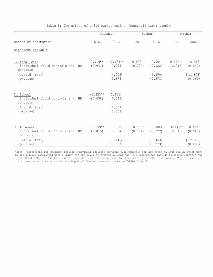
Table 5: The effect of child market work on household labor supply

Children Father Mother

Method of estimation OLS 2SLS OLS 2SLS OLS 2SLS

Dependent variable 1. Total work 0.919** -0.164** 0.008* 0.004 0.113** -0.015

(individual child controls and) HH controls

(0.041) (0.075) (0.004) (0.022) (0.016) (0.049)

[Overid. test] [4.008] [6.470] [11.878] (p-value) (0.676) (0.373) (0.065)

2. School -0.451** 0.131*

(individual child controls and) HH controls

(0.038) (0.076)

[Overid. test] 2.553 (p-value) (0.863)

3. Idleness -0.139** -0.025 -0.008* -0.003 -0.112** 0.006

(individual child controls and) HH controls

(0.015) (0.064) (0.004) (0.022) (0.016) (0.049)

[Overid. test] [0.745] [6.463] [12.309] (p-value) (0.993) (0.373) (0.055)

Notes: Regressions for children include individual children controls plus controls for age minus maximum age by which work is not allowed interacted with a dummy for the level of minimum working age. All regressions include household controls and state fixed effects. Overid. test is the over-identification test for the validity of the instruments. The statistic is disitrbuted as a chi-square with six degree of freedom. See also notes to Tables 3 and 4.

Table 6: The effect of child market work on household labor supply – 2SLS estimates Robustness checks

Children Father Mother

Dependent variable

1. Total work (age 10-15) -0.378** 0.038 0.025

(0.164) (0.046) (0.114) [Overid. test] [2.380] [5.060] [6.877] (p-value) (0.882) (0.536) (0.332)

2. Total work (age 10-18) -0.147** 0.014 -0.041

(0.042) (0.013) (0.028) [Overid. test] [10.667] [2.868] [11.061] (p-value) (0.099) (0.825) (0.086)

3. Market work -0.083 0.058 -0.003

(0.072) (0.041) (0.047) [Overid. test] [2.575] [2.059] [6.657] (p-value) (0.860) (0.914) (0.354)

4. Work in HH farm -0.081** -0.054 -0.012

(0.035) (0.036) (0.019) [Overid. test] [6.338] [1.872] [9.698] (p-value) (0.386) (0.931) (0.138)

5a. Total work – effect of boys market work -0.197* -0.006 -0.108 (0.113) (0.037) (0.078) 5b. Total work – effect of girls market work -0.135* 0.014 0.038 (0.080) (0.027) (0.060)

[Overid. test] [11.583] [9.728] [18.470] (p-value) (0.480) (0.640) (0.102)

6. Total work –States with Compulsory school age 16 -0.124* 0.006 -0.025

(0.068) (0.024) (0.048) [Overid. test] [1.240] [0.392] [10.083] (p-value) (0.538) (0.822) (0.006)

7. School enrollment–States with Compulsory school age 16 0.120 (0.077) [Overid. test] [1.355] (p-value) (0.508)

8. Total work – Households with one child only 0.007 0.023 (0.028) (0.059) [Overid. test] [3.930] [8.667] (p-value) (0.686) (0.193)

9. Total work –state specific age profiles -0.123* 0.007 0.031 (0.073) (0.023) (0.051) [Overid. test] [3.425] [4.659] [8.154] (p-value) (0.331) (0.588) (0.227)

Notes: Specification 8 controls for the interaction of following variables with state dummies: father and mother age and age squared, average age of children 10-16, child age (this variable only in children regressions). Specification 9 controls for the average age of children at or above legal working age in minus maximum age by which work is not permitted in the state of residence. See also notes to Table 5.

Table A1: Distribution of children age in 1910 and 1920

Mother birth cohort

Mother age in 1920

cumulative % of mothers born 1870-1895

cumulative % of mothers with cohabiting children

born before 1904

Difference

1910 1920 1910 1920 1920-1910 1885 35 7.726 7.976 17.833 14.632 3.202 1884 36 15.471 15.746 21.307 16.850 4.457 1883 37 22.666 22.963 24.647 19.593 5.055 1882 38 30.816 31.301 29.284 23.240 6.044 1881 39 37.508 38.829 32.836 26.446 6.390 1880 40 45.427 47.645 37.029 30.173 6.856 1879 41 50.854 53.162 39.569 32.430 7.140 1878 42 57.846 60.120 42.980 35.315 7.665 1877 43 63.828 65.961 45.915 37.384 8.530 1876 44 69.668 71.407 48.464 39.356 9.108 1875 45 75.702 77.620 51.037 41.607 9.431 1874 46 81.392 82.530 53.241 43.255 9.986 1873 47 86.085 87.178 55.053 44.736 10.317 1872 48 91.385 91.821 57.042 46.181 10.862 1871 49 95.570 95.731 58.397 47.338 11.059 1870 50 100.000 100.000 59.793 48.458 11.335 Notes: a mother is defined as a woman with a child born between 1904 and 1910, i.e. aged 10-16 in 1920.

Figure 1

Child labor by minimum legal working age

MWA==0

0

.3

.6

MWA==7 MWA==8

MWA==12

0

.3

.6

MWA==13

10 12 14 16 18

MWA==14

10 12 14 16 18MWA==15

10 12 14 16 180

.3

.6

Notes: MWA is Minimum legal working age.

Figure 2

Child labor by minimum legal working age: actual and estimated

MWA==0

0

.3

.6

MWA==7 MWA==8

MWA==12

0

.3

.6

MWA==13

10 12 14 16 18

MWA==14

10 12 14 16 18MWA==15

10 12 14 16 18

0

.3

.6

Notes: See notes to Figure 1.

Figure 3

Household labor supply with no altruism

s w1

w2

w2=α(w1-s)/(2-α)

w2=(1+α)w1/(1-α)+s

e1>0 e2>0

e1>0 e2=0

e1=0 e2>0

s

Figure 4

Household labor supply with altruism

s w1

w2

w2=w1-s e1>0 e2>0

e1>0 e2=0

Figure A1

Labor force participation by age in states with minimum legal working age 12 and 14

MWA=12 MWA=14

10 20 30

0

.2

.4

.6

.8

Notes: See notes to Figure 1.