Embed Size (px)
Citation preview

This paper can be downloaded without charge at:
The Chicago Working Paper Series Index:http://www.law.uchicago.edu/Publications/Working/index.html
The Social Science Research Network Electronic Paper Collection:http://papers.ssrn.com/paper.taf?abstract_id=160530
CHICAGOJOHN M. OLIN LAW & ECONOMICS WORKING PAPER NO. 60
(2D SERIES)
How Dramatically Did Women’s SuffrageChange the Size and Scope of Government?
John R. Lott, Jr., and Larry Kenny
THE LAW SCHOOLTHE UNIVERSITY OF CHICAGO
How Dramatically Did Women’s SuffrageChange the Size and Scope of Government?
John R. Lott, Jr. and Larry Kenny1
It is not really surprising that this welfare state should breed apolitics not of “justice” or “fairness” but of “compassion,” whichcontemporary liberalism has elevated into the most important civicvirtue. Women tend to be more sentimental, more risk-averse andless competitive than men—yes, it’s Mars vs. Venus—and thereforeare less inclined to be appreciative of free-market economics, inwhich there are losers as well as winners. College-educatedwomen—the kind who attend Democratic conventions—are alsomore “permissive” and less “judgmental” on such issues ashomosexuality, capital punishment, even pornography.
Irving Kristol, “The Feminization of the Democrats,”The Wall Street Journal (September 9, 1996): p. A16
Citing marriage as “a very important financial divider,” theAmerican Enterprise Institute's Doug Besharov suggests moremarried women did not vote for Dole because of a widespread senseof societal insecurity: “It is not that they distrust their husband, butthey have seen divorce all around them and know they could benext.” The Polling Company's Kellyanne Fitzpatrick is categorical:“Women see government as their insurance.” (Perhaps significantly,of the 24 million individuals working in government and in semi-governmental non-profit jobs, 14 million—58 percent—are women.)
The Richmond Times Dispatch, December 5, 1996
For decades we have known that women vote differently thanmen. In the presidential elections from 1980 to 1996 the gendergap—the difference between the way men voted and the waywomen did—was: 14 points in 1980, 16 in 1984, 15 in 1988, 5 in1992, and 17 in 1996 (Langer, November 8, 1996). According toVoter News Service election day exit polls, if men alone could havevoted in the 1996 presidential election, Robert Dole would havebeen elected president by carrying 31 states. We know that the 1 University of Chicago Law School, and University of Florida Department ofEconomics.

Chicago Working Paper in Law and Economics 2
differences between men and women extend to even such things astheir sources of news, with women relying predominantly ontelevision and men on newspapers and radio (Nando News July 30,1996).
Disciplines such as sociobiology emphasize why the differentsexes develop distinct behavioral patterns consistent with maximizingtheir probability of successfully passing on their genes (Trivers, 1985,p. 20).2 While sociobiology discusses this theory across many species,a large psychology literature focuses more specifically on humans.This research finds that men are more likely to take career risks andmore single-minded about acquiring resources,3 while “women aremore inclined to be nurturing and orientated towards others withgreater attachment towards their children and less willing to tradematerial resources for time spent with their children or in otheractivities” (Browne, 1995, p. 980 and see also Epstein, 1992, pp.986-995).
Many feminists argue that this different perspective arises, atleast in part, from “their sexuality,” and provides a reason forincluding women in the political process (Gilligan, 1982, p. 129).4Men can not be expected to see things the same way that womendo. “[T]he disappointment of suffrage is recorded in the . . .tendency of [some women] in voting only to second their husbands’opinions” (Gilligan, 1982, p. 129). To these women, it would beshocking to think that suffrage did not alter the outcomes of thepolitical process.5,6
2 For example, males’ ability to reproduce often depends upon them beingwilling to take more risky strategies in order to acquire resources or otherwiseimpress females. For males, the payoff for being the winner is high, as he canthen sire many children. While all the females in a herd of animals will havean opportunity to mate, for many species it is frequently only a few percent ofthe males who sire offspring. To the extent that this strategy is imprinted atthe genetic level, it might not be too surprising that males and females haveinnately different attitudes towards risk.3 Social biologists have long predicted that the sex making the smallestparental investment would gain from taking relatively riskier strategies.4 See also Chodorow (1978) for related discussions on this topic.5 Many women who fought for suffrage felt the same way. For example, seeLewis (1987, pp. 141-158).

3 Women’s Suffrage and the Size of Government
Yet, why these differences would affect the views of what rolegovernment should play is not completely clear. The first quote byKristol raises some interesting possibilities. Maybe, as thesociobiologists and psychologist argue, women are more risk-aversethan men, but why do women choose to use the government ratherthan other mechanisms to provide insurance? Many types ofgovernment programs are primarily wealth transfer programs ratherthan insurance programs in the normal sense.
Marriage also provides another economic basis for men andwomen preferring different policies. It typically encourages men toaccumulate market capital and leads women to acquire householdskills and shoulder most of the child rearing responsibilities. Whilethe gains from marital specialization and from efficient statisticaldiscrimination in the labor market can be internalized throughmarriage, divorced women are unable to recoup the fullcompensation for their family-specific investments, and singleworking women lose from labor market discrimination (see Huntand Rubin, 1980). Hence, single women as well as women whoanticipate that they may become single may prefer a more progressivetax system and more wealth transfers to low-income people asalternative to a share of a husband’s uncertain future income.
Others have noted that at least in some countries governmentjobs are filled primarily by women (e.g., see Rosen, 1996, discussingSweden). Today women make up 54.8 percent of the U.S. Federalgovernment white collar workers. Thus, women may feel that theyhave more at stake the government remaining the same or growing(Stark, 1996, p. 78). Possibly, it is even more specific. Men andwomen may support those government activities where they aremore heavily employed (e.g., defense and education, respectively).
One long standing puzzle facing public choice has been whygovernment growth started when it did (Tullock, 1995). In theUnited States, many have noted the general problem: “There wastremendous expansion of government growth in the 1930’s, to besure, but that expansion is better seen as a continuation of the
6 Strauss (1992, p. 1012) discusses the tensions feminists face in arguing thatthere are “biological or otherwise deep-seated differences between men andwomen.” If they acknowledge these differences, to what extent might thesearguments then be used against moves to equality in other areas?

Chicago Working Paper in Law and Economics 4
expansion of the scope of government in the 1920’s” (Holcombe,1997, p. 26). The literature is littered with theories from theunbalanced growth hypothesis (Baumol, 1967), ratcheting effects(Peacock and Wiseman, 1961), revenue maximizing bureaucrats(Niskanen, 1971), reductions in the costs of collecting taxes (Kauand Rubin, 1981), entrepreneurial politicians (Becker, 1985 andLott, 1990 and 1997), the development of interest groups(Holcombe, 1997), and the notion that government is a superiorgood (Wagner’s Law).7 All these theories face one significantproblem: government has not always been growing. Previous generaldiscussions involving the extensions of the voting franchise (e.g.,Meltzer and Richard, 1978, 1981, and 1983) also have problemsexplaining the timing of growth. Indeed in the United States, withthe exceptions of wars, real per capita Federal Governmentexpenditures remained remarkably constant until the 1920’s. In fact,as has been widely noted by public choice scholars, World War I wasthe first war after which per capita government expenditures did notreturn back to their pre-war levels and by the end of the 1920’s thegrowth trend that we are so familiar with today had begun.8 Toexplain this timing, some point to the effect that the seeminglysuccessful economy wide regulations during the war had on people’sbeliefs about the role of government (Higgs, 1987).
We propose that giving women the right to vote changed thesize of government. We examine several indcators of the size andscope of government, from state government expenditures andrevenues to voting index scores for Federal House and Senatemembers from 1870 to 1940.
Twenty-nine states gave women the right to vote before the19th amendment to the Constitution was approved in 1920, withseven of the remaining nineteen approving the amendment andtwelve having women’s suffrage imposed on them. Womenobtained the right to vote in four states even prior to the turn of thecentury, in eight states between 1910 and 1914, and in 17 states in
7 For an extensive survey of Wagner’s Law see Bennett and Johnson (1980).8 Another argument claims that larger government has resulted fromincreasing income equality and education (Peltzman, 1980). See Lott (1990) fora response to the claims regarding education.

5 Women’s Suffrage and the Size of Government
1917-19. By 1940, the end of our sample, women had been votingin 12 states for at least 26 years and in 4 states for at least 44 years.
Although a number of women took advantage of their newright to vote immediately, it took several decades for turnout to fullyadjust. We find the growth in female voter turnout to be positiveassociated with teh expansion of government. Since suffrage wasgranted to women in different states over a long period of timeextending from 1869 to 1920, it is unlikely that World War I is thekey. These data also allow us to address causality questions in unusualways. The central issue is: did giving women the right to vote causegovernment to grow or was there something else which bothcontributed to women getting the right to vote and also increasedgovernment growth? We find very similar effects of women’ssuffrage in states that voted for suffrage and states that were forcedto give women the right to vote, which suggests the second effect issmall.
The remaining empirical analysis utilizes more recent pollingdata to help explain why women and men vote so differently. Wefind that there is a greater gender gap for single mothers, and thatwomen—particularly single women—are more likely to be liberaland a Democrat and to have voted for the Democrat presidentialcandidate.
II. Examining the PoliticalDifferences between Women and Men
“Although many media accounts still suggest that the gender gap isgreatest on ‘women’s issues,’ in fact the gulf today tends to be onissues involving the existence and expansion of the social-welfarestate.”
Steven Stark, “Gap Politics,”Atlantic Monthly, July 1996, p. 72.
Why would men and women have differing political interests?Starting with the simplest case as a comparison: if there were nodivorces in society and women and men married early in life, theinterests of men and women would appear to be closely linked
Chicago Working Paper in Law and Economics 6
together.9 However, as divorce or desertion rates rise, more womenwill be saddled with the costs of raising the children.10 Divorcedwomen may seek legal guarantees to some portion of this expectedhigher income through alimony, but, besides difficulties in trackingdown the man to ensure payment, relatively risk averse women mayin addition prefer some guaranteed minimum income over the riskyreturn from the particular man that they were originally married to.While the evidence indicates that welfare leads some fathers todesert their families, some women may also view welfare as a meansof allowing them to remain at home and raise their children whentheir husbands leave them.
The relative investments women and men make in householdproduction versus careers also plays a role. Take the limiting casewhere women make investments in the family and men investmentsin their careers. As the divorce rate rises, women’s expected ability tointernalize these men’s early investments in their careers declines.Some women may acquire skills that will be useful in themarketplace outside the family, and they will make fewer householdinvestments. Even ignoring the lost family-specific sunkinvestments and the costliness of the marriage market, such thingsas the growing age differential between men and women in latermarriages make remarriage appear to be somewhat less satisfactoryfor women then for men, possibly in part because age differentiallyaffects their abilities to have children. (Presumably, on average thisfact is taken into account in the initial marriage market competition,and women are compensated at that point.) Again women face twooptions, either relying on some share of the husband’s relatively risky
9 Of course, this linkage might not be perfect because views might not only bea function of current costs and benefits but also the biologically hardwiredattitudes, for example, towards risk which evolved over the eons.10 This might arise because if the old biological forces, discussed in theintroduction, assert themselves with some men leaving the relationship afterthe women have born children. If men are trying to maximize the rate atwhich they pass on their genes, they will try to find younger still fertilewomen as their spouses age. Indeed while men are older than women whenthey marry, the age gap is larger for those entering into their second and thirdmarriages than it is for those in their first marriage. For first marriages the agegap is 3 years, for second marriages it is 5, and for third marriages 8. (SeeBrowne, 1995.)

7 Women’s Suffrage and the Size of Government
future earnings (assuming that those earnings can be attached) orsome guaranteed minimum income.
Our earlier discussion on the differences between men andwomen appear to suggest two other reasons why women, onaverage, would favor a more progressive tax system and more wealthtransfers to lower income people.11 First, is the claim “that men aremore single-minded about acquiring resources than women.”12
While many women will be married to these men and while manywill gain through inheritance,13 it would appear that men, simplybecause some of them will be single when they earn and spend thisincome, might be discriminated against by a progressive income tax.Second, if women are more willing to “trade material resources fortime spent with their children,”14 women by consuming untaxedactivities are going to avoid some of the burden of the tax.
Differences in women’s and men’s views toward wealthtransfers, even if true on average, are unlikely to be monolithic andare likely to vary over time as the divorce rate and personalcharacteristics such as marriage and children change. The conflictswithin the ranks of women or men seem obvious: women whoremain married to successful men would oppose such transfers, butunsuccessful men and their spouses and divorced and single womenwould support them. Indeed there is already some cross-sectionalempirical evidence that supports this conclusion. Hunt and Rubin(1980) find that it is the number of single women—not the femalelabor force participation rate as one might suspect if employmentdiscrimination were the real concern—that determined what stateswere most likely to pass the Equal Rights Amendment during the1970s.15
11 International polling data find that women tend to be relatively risk averse“almost” everywhere (see Stark, 1996, p. 75).12 Browne, 1995, p. 980.13 Because of inheritance, this effect may be partially offset by the longer lifeexpectancy of women.14 Browne, 1995, p. 980.15 If men and women do indeed benefit differentially from government policy,their political positions should depend not only upon their own sex but alsothat of their children. Women with male children and men with femalechildren will find it more in their interests at the margin to supportgovernment policies that favor the other sex. Similarly parents (particularly
Chicago Working Paper in Law and Economics 8
III. Changes in Voting LawsA great expansion of voting rights has occurred over the last
century and a half, with a corresponding shift in political power. It isimportant to account for these and other changes in voter turnout sothat we do not falsely attribute changes in voting participation ratesto female suffrage when other changes may have been occurringaround the same time. This information will also allow us toexamine whether it is an increase in the franchise per se that isproducing higher government expenditures or whether extendingthe franchise to women was in some way unique. Table 1 describeshow the various legal restrictions on voting changed over time. Ourvoter turnout, state government spending, and federal legislativevoting data were collected beginning in 1870 or when a stateentered the union, whichever is later, so the first column lists eachstate’s year of entry. The one exception is Arizona, whose stateexpenditure and revenue data are available for 1911.
Adopting secret ballots prevented many illiterate citizens fromvoting; reading skills were required when voting no longer involvedsimply taking a colored card that represented one’s party preferenceinto the voting booth. Secret ballots also greatly hampered votebuying, since it was much more difficult for those buying votes tomonitor which candidates a person voted for. The first columnillustrates how the secret ballot swept through the country, with 40states adopting it between 1888 and 1896 (See Anderson andTollison (1990) and Heckelman (1995)).
The timing of women’s suffrage is shown in column 2.Women obtained the right to vote in four states even prior to theturn of the century, in eight states between 1910 and 1914, and in17 states between 1917 and 1919.
As shown in column 3, the poll tax was used by 16 states atsome point during our sample period. During this time, the tax wasimposed in 10 states, eliminated and reimposed in 2 states, andeliminated in 8 states. By 1940, for 5 states at least 20 years hadelapsed since the poll tax had been repealed. single parents) with children of the same sex as themselves will obtain an evengreater return to political activity. Altruism towards siblings could alsocomplicate this picture. In any case, using a person’s own sex is an imperfectmeasure of one’s political preferences.
9 Women’s Suffrage and the Size of Government
The last column depicts states’ reliance on the literacy test.Nineteen states used this restriction at some time during the period.
IV. Effect of Suffrage on Spending and TaxationUsing state government expenditure and revenue data for all 48contiguous states from 1870 to 1940, it is possible to study theimpact of women’s suffrage on the size of government. Theexpenditure and taxation data prior to 1915 were provided by JohnWallis. Subsequent data were obtained from various issues ofFinancial Statistics of States. Since the series from both sourcesneeded to be comparable, analysis of taxation and expenditure wasrestricted to series satisfying that criterion: total expenditure(TOTAL EXPENDITURE), total revenue (TOTALREVENUE), property tax revenue (PROPERTY TAX), currentand capital expenditures on elementary and secondary schools andlibraries (EDUCATION), current expenditures on charities,hospitals, and corrections (SOCIAL SERVICES), and current andcapital expenditures on highways (HIGHWAY) (see Table 2).16
Given that most serious crime is committed against males and thatwomen may be more likely to value spending on charities,aggregating these different types of spending together under thelabel of social services is less than ideal. These variables are in real(1967) dollars per capita. These data were checked thoroughly, andsuspicious data from the earlier period were deleted.17 Spending ortaxation had to be at least twice or less than half that of surrounding
16 Although we were unable to replicate exactly the data on TOTALEXPENDITURE from Wallis using Financial Statistics of States, the figures forthe two series seemed close enough to permit analysis.17 The deleted data included: TOTAL EXPENDITURE: DE 1888, IN 1889,KS 1877, KY 1882-83, MD 1903, MA 1939, MS 1939, ND 1939, NH 1939,NJ 1939, SC 1877 - EDUCATION: CA 1908; IN 1875-77, 1879, 1884,1901; KY 1897; MD 1871; SC 1877 - SOCIAL SERVICES: FL 1871-72;KY 1882-83; OH 1912; SC 1877 - TRANSPORTATION: none - TOTALREVENUE - DE 1887, 1891; ID 1912; IN 1889; IA 1905; KY 1873; NV1880; NY 1874; PA 1877; SC 1877; TN 1875; TX 1885; WA 1896; WV1895; WY 1893, 1899 - PROPERTY TAX: AL 1911, AR 1908; TN 1879;UT 1905; WV 1895; WY 1893. We also tried deleting all the spending andrevenue data from Washington for 1907-14, but this did not alter our basicfindings.

Chicago Working Paper in Law and Economics 10
years to warrant deletion, though this does not affect the results wereport.18
Figure 1 provides a simple graphic illustration on therelationship between women’s suffrage and the percent of the totalpopulation over age 21 that voted. All state dates are normalized sothat year zero on the horizontal axis is the first year when women ina state were allowed to vote. Values to the right along the bottomaxis shows the number of years following suffrage, and values to theleft indicate the number of years prior to the adoption of the law.While Figure 1 does not control for any other factors that mightinfluence the returns to voting, the graph is very suggestive. Onaverage voting participation rates were very stable in the yearspreceding suffrage. Yet, once suffrage was granted, participationrates immediately rose from 25 to 37 percent, with a continuedslower rise to 43 percent occurring over the subsequent decade. Tothe extent that voting by women reduces the return to men voting,the simple increase in the percent of the population votingunderestimates the number of women who vote. The appendixprovides a more systematic investigation of the factors affectingparticipation rates during these years.
Figure 2 graphs the simple relationship between the granting ofwomen’s suffrage and per capita state government expenditures andrevenue. The bottom axis is the same as that used in Figure 1, and itsets year zero as the fiscal year during which women first voted inany state.19
18 We ended up deleting only about 6 observations per regression. While ithad virtually no effect on the expenditure results, including these observationsslightly increased the size of female suffrage’s impact on state governmentrevenue. For example, reestimating the results that we will be reporting inTable 3 with these additional observations implies that the impact of additionalturnout due to female suffrage on total state government expenditures is .8297(t-statistic = 2.661) and on total state government revenue is .8222 (t-statistic =2.691).19 Because state expenditures and revenues were missing for some years, thechanges in the average state’s values between years were calculated for thosestates which had values in both adjacent years. When a state is missing nomore than one consecutive year of data, the change between the two years forwhich the data is available is calculated and then divided by 2. These changeswere linked to the average expenditure and revenue levels in the eleventh year

11 Women’s Suffrage and the Size of Government
Figure 1: The Effect of Giving Women the Right to Vote on The
Percentage of the Adult Population that Votes
0
0.05
0.1
0.15
0.2
0.25
0.3
0.35
0.4
0.45
0.5
-10 -5 0 5 10
Years Before and After Women Were Given the Ri ght to Vote in Different
States: Year Zero is the First Year that Women Were Allowed to Vote in Different
States
The
Per
cent
age
of th
e O
ver
21 Y
ear
Old
Pop
ulat
ion
that
Vot
ed
after suffrage was enacted. Graphing the means for the observed stateexpenditures and revenues in each year produces a very similar graph.

Chicago Working Paper in Law and Economics 12
Per Capita StateExpenditures
Per Capita State Revenue
0
50
100
150
200
-10 -5 0 5 10
Years Before and After Women Were Given the Right to Vote in Different States: Year Zero is the First Year that Women Were Allowed to Vote in Different States
Rea
l Per
Cap
ita 1
996
Dol
lars
Figure 2: The Effect of Giving Women the Right to Vote on Per Capita State
Government Expenditures and Revenue
13 Women’s Suffrage and the Size of Government
While some caution is needed in reading this graph—asnothing else is being controlled for—the figure illustrates thedramatic change in state governments when women were given theright to vote. State government expenditures declined for four of thefive years before women began voting and expenditures reach theirlowest point immediately before women were given the right tovote. Within four years after women’s suffrage, expenditures hadrisen above their previous peak and, within eleven years, real percapita expenditures had more than doubled from $101 to $208.20
Given that the vast majority of spending for the fiscal year thatcoincided with “year zero” was decided immediately before womenwere allowed to first vote, it appears that legislators started approvingincreased spending only after women began to vote. This timingprovides some evidence that the causation primarily runs from givingwomen the right to vote to larger government—as opposed to someleft-out variable (e.g., a general change in values) which bothresulted in women’s suffrage and increased government spending.21
We will return to the question of causation in Section VI.One concern with Figure 2 is that many states made the
decision to let women vote around World War I and that the war,rather than suffrage, may have prompted higher governmentexpenditures.22 Since the war ended in November 1918 and the19th Amendment was ratified in August 1920, examining just thenineteen states that extended suffrage as a result of the Amendmentallows us to see whether state governments started expanding due tothe war and not suffrage. As shown in Table 1, this group of statesincluded states from across the nation—most of which were notmembers of the old Confederacy (e.g., Connecticut, Delaware,
20 By comparison, 1994 per capita state government expenditures in 1996dollars averaged $3,177.21 This result is quite consistent with more recent evidence that congressmenand senators do not alter their voting behavior when they face a new set ofconstituents—either due to running for another office or due to redistricting(see Lott and Bronars, 1993 and Lott and Davis, 1992).22 Of the 19 states where women voted for the first time in 1920, seven hadstate legislatures which approved the amendment (KY, MA, NH, NJ, NM,PA, WV) and twelve did not (AL, CT, DE, FL, GA, LA, MD, MS, NC,SC, VT, and VA). Figure 3 was put together in the exact same manner asFigure 2 described in footnote 29.

Chicago Working Paper in Law and Economics 14
Kentucky, Massachusetts, Maryland, New Hampshire, New Jersey,New Mexico, Pennsylvania, Vermont, and West Virginia). Figure 3provides equally dramatic evidence that state governments did notstart expanding as a result of either the beginning or end of the war,but only once women were given the right to vote. Unfortunately,only one state had expenditure data and no states had revenue datafor 1920, so the values shown in the figure for 1920 are essentiallythe average change from 1919 to 1921. While we are not able topinpoint exactly when state government spending and revenueincreased, state government expenditures continued to decline for aleast one year after the war was over, which suggests that thesubsequent increases were not due to the war.
World War I appears to have had little noticeable impact onstate governments, as the slight downward trend in state per capitaspending and revenue that started in 1913 continues through 1919and is remarkably similar to the pre-suffrage pattern observed in thefull sample. If anything, the slightly greater explosion in governmentspending shown in Figure 3 may explain part of the reason whythese states were the most reluctant to extend suffrage.
Obviously other socioeconomic variables must be accounted forwhen we attempt to explain changes in government revenue orspending. Data on illiteracy rates, foreign born population, male andfemale populations aged 21 or older, the percent of the workforce inmanufacturing, and real manufacturing wages were obtained fromthe eight censuses conducted during this period.23 Our business cyclemeasure was (ACTUAL GNP/TREND GNP).24 The HistoricalStatistics of the United States: Colonial Times to 1970 providedconsistent decennial series on: total population, rural and elderlypopulations, and on the number of female gainful workers. 23 We also tried using the real average value per farm and a very crude measureof per capita personal income based on two sources, but this produced verysimilar results to those we show. Since the government series on state personalincome goes back only to 1929, a crude measure of per capita personal incomewas created by combining the government figures for 1930 and 1940 with dataon 1880, 1900, and 1920 from Lee, Miller, Brained, and Easterlin (1957).Interpolated estimates for 1890 and 1910 and extrapolated estimates for 1870were created taking into account changes in U.S. GNP over these years.24 This was constructed from GNP data reported in Historical Statistics of theUnited States: Colonial Times to 1970.

15 Women’s Suffrage and the Size of Government
Per Capita StateExpendituresPer Capita State Revenue
Figure 3: The Effect of Giving Women in the Right to Vote on Per Capita State Government
Revenue for Only Those States Which Gave Women the Vote in 1920
50
100
150
200
250
1910 1915 1920 1925 1930
Years Before and After Women Were Given the Right to Vote in Different States: 1920 is the First Year Women Were
Allowed to Vote in This Set of States
Rea
l Per
Cap
ita 1
996
Dol
lars

Chicago Working Paper in Law and Economics 16
Interpolation was also used to create inter-census estimates forall the socioeconomic variables. State dummies capture time-invariant cross-sectional differences in amenities, “tastes” forgovernment, and institutional structure. The year dummies pick upchanges over time in the relative price of government services, federalprograms, national business cycle conditions, and “tastes” forgovernment programs. However, the use of fixed state and yeareffects also has its drawbacks: while it may correctly measure left-outvariables, it may falsely cause us to attribute some changes ingovernment growth to fixed effects that should be attributed tovariables like women voting.
Table 3 provides our first estimates of the effects of givingwomen the right to vote and of imposing and removing poll taxes.The specification regresses our estimated effects of women’s suffrageon voter turnout from the appendix on measures of stategovernment total expenditures and revenue. The coefficients for afemale suffrage dummy, time since suffrage, and time since suffragesquared reported in Table A.1 specification 6 were used to create ameasure of ADDITIONAL TURNOUT DUE TO FEMALESUFFRAGE.25 The estimates imply that after women were giventhe right to vote, voter turnout increased immediately and then grewsteadily for many years. Similarly the coefficients from the sameregression in the appendix on 1) poll tax, 2) a dummy indicatingwhether a poll tax has been removed, 3) time since removal of thepoll tax, and 4) time since removal squared have been multiplied bytheir variable values, creating an estimate of ADDITIONALTURNOUT DUE TO POLL TAX. With the exception ofPROPERTY TAX (1230 observations), these regressions are basedon 1541 to 1876 observations.
Granting women the right to vote is estimated to raise totalspending and revenue. In Table 3, ADDITIONAL TURNOUTDUE TO FEMALE SUFFRAGE has significantly positivecoefficients in the total expenditure and total revenue regressions butnot in the other four regressions. Our voter turnout regressionsimplied that in a typical state, where 46 percent of the adultpopulation is female, suffrage resulted in an immediate 17.5percentage point increase in the fraction of the adult population 25 The other estimates of turnout produced similar results.

17 Women’s Suffrage and the Size of Government
voting and in increases of 26 percentage points after 25 years and 33percentage points after 45 years. Based on these estimates, grantingwomen the right to vote caused expenditures to rise immediately by16 percent (.175_.845 increase in log), by 24 percent after 25 years,and by 31 percent after 45 years. Similarly, female suffrage led to a 22percent rise in revenue after 25 years and a 28 percent rise after 45years.
Table 4 reports a simple dummy for whether women wereallowed to vote times the fraction of the population over 21 that isfemale (FEMALE SUFFRAGE * FRACTION OFPOPULATION OVER 21 FEMALE) and a dummy variableindicating whether a poll tax was in effect (POLL TAX). Theinteraction between the suffrage dummy and the percent female isused because the impact of suffrage on turnout depends upon howmany women there are in the population. In the extreme, obviouslyif there were no women, enacting suffrage would not increase thepercent of the adult population that voted, and thereby the size ofgovernment.
The results for the simple specification in Table 4 are consistentwith the evidence in Table 3. Female suffrage has a significantimpact only on total spending and revenue. Granting women theright to vote is estimated to raise total expenditure and revenue by 13percent on average in our sample. Recall that the median stategranted suffrage in 1918 and that our data do not extend past 1940.However, Tables 3 and 4 also produce a puzzle, but not sufficientdata for an answer: what revenue and spending categories areincreasing? Total spending and taxes are rising, but the componentsthat we so far have been able to measure do not change much. Thepoint estimates for social service expenditures are large and positive,and imply that these expenditures are increasing at least at half therate of the increase in total expenditures in response to the growinginfluence of female voters. However, the coefficients are onlystatistically significant when the fixed year effects are replaced with aquadratic time trend. Unfortunately, the one tax category and threespending categories are not important enough to capture the majortrends in taxes and spending. In this sample, property taxes are only26 percent of state revenue and the three categories of spending thatwe can measure (education, social services, and transportation)account for just 41 percent of total expenditures.
Chicago Working Paper in Law and Economics 18
Because of data limitations Tables 3 and 4 do not examine theincreases for omitted revenue sources like income, poll, business, orsales taxes or for omitted expenditures on police, insurance trusts,natural resources, interest costs, higher education, regulation, oradministration that are correlated with giving women the right tovote. Fortunately, some evidence of total state governmentexpenditures by type are available from the Historical Statistics of theUnited States: Colonial Times to 1970 for 1902, 1913, 1922, and1927. Table 5 lists all the different components of expenditures.Over this period the eight largest absolute increases in per capita stateand local government expenditures in real 1996 dollars were:education, $110; highways, $96; state government transfers to localgovernment, $33; interest on general debt, $28; “other” generalexpenditures, $24; utilities, $19; sanitation, $12; and hospitals, $11.The influence of female voters may have been reflected in the largeincreases in education, sanitation, and hospital expenditures by localgovernments and the large increase in state transfers to localgovernments, which spend over a quarter of their budgets oneducation. Our inability to document the influence of women’ssuffrage on state education expenditures may be due to the very smallrole that state support played in education funding.
There is also the issue of whether higher state governmentexpenditures are merely substituting for reduced expenditures at thelocal level. If giving women the right to vote merely transferredgovernment operations from the local to the state level, it would bedifficult to argue that suffrage was responsible for larger government.Table 5 demonstrates that this is not the case. While total per capitastate government expenditures in real 1996 dollars rose from $42 in1902 to $154 in 1927, local government spending also rosedramatically over the same period: $219 to $478.The evidence is also weakly consistent with past work on the polltax. Filer, et al. (1991) and Husted and Kenny (1997) show that polltaxes reduced voter turnout, particularly among the poor. As a result,the new pivotal voter had a higher income and should prefer lessredistribution to the poor. This hypothesis is supported by evidencein Table 4 that it resulted in lower total spending and total revenue.On the other hand, the significant and negative coefficient onADDITIONAL TURNOUT DUE TO POLL TAX and thesignificantly positive coefficients on POLL TAX in the SOCIAL

19 Women’s Suffrage and the Size of Government
SERVICES regressions are not consistent with this hypothesis,though this interpretation is complicated by the inclusion of prisonexpenditures into this measure. The poll tax lowered turnout, whichis estimated to raise spending on hospitals, charities, and prisons.Similarly, the results in Tables 3 and 4 showing that the poll taxlowered spending on education are not consistent with both the polltax reducing voter turnout among the poor and the evidence thatpublic education creates transfers to middle and upper incomefamilies (Stigler, 1970 and Lott, 1987). The poll tax is also associatedwith greater reliance on property taxes in Table 3.
Similarly, the literacy test was supposed to keep the illiteratefrom voting, again producing a new pivotal voter who preferred lessredistribution than the old pivotal voter. The literacy test, however,also was used to keep immigrants with poor language skills fromvoting and to discriminate against blacks. Husted and Kenny (1997)find only weak support for the literacy test having a negative impacton welfare spending. The results in Table 3 do not support thatevidence. Indeed, we find that the test raised social service spending(charities, hospitals, prisons). It was also associated with higherspending on education, higher total revenues (but not totalexpenditure), and lower highway budgets.
The secret ballot made it more difficult to monitor voting andthus greatly hampered vote buying. If the rich purchase votes tothwart income redistribution, Anderson and Tollison (1990)hypothesize that secret ballots should result in more incomeredistribution and thus greater spending. The secret ballot dummyvariable is, however, not significant in these regressions.
Motor vehicle registrations per capita (MOTOR VEHICLEREGISTRATIONS) track the rise in highway budgets as theautomobile grew in popularity.26 It has the expected positive impacton highway spending.
Salaries are higher in urban areas, which primarily compensatesfor the higher cost of living. Since the price elasticity forgovernment services is less than one, this should result in highergovernment spending. The significant and positive coefficients on 26 Passenger Cars and Motor Trucks Combined (includes road tractors after1923). U.S. Dept. of Commerce, Bureau of the Census, Statistical Abstract of theUnited States . (various years, various editions).
Chicago Working Paper in Law and Economics 20
LOG DENSITY in the total spending and revenue and educationand social services expenditures regressions support this hypothesis.Similarly, total spending and revenue fall as the fraction living inrural areas (RURAL) increase; the significantly positive coefficientin the EDUCATION regression is puzzling.
The log of state population (LOG POPULATION) is utilizedto capture economies of scale at the state level. The negativecoefficients are consistent with economies of scale, but theelasticities between 2 and 6 seem implausibly large. Our businesscycle measure (ACTUAL GNP/TREND GNP) adds little to thetime dummies that are in the regressions. This variable is neversignificant.
An increase in either the fraction of the population that is blackor the fraction 65 or older is associated with a rise in the potentialpopulation who depend on assistance and a fall in per capita income.Although there are some exceptions to this pattern, on net theincome effect appears to dominate. Significantly negativecoefficients are found for percentage black or elderly in threeregressions.
Five variables are included to capture differences in income.Multicollinearity is likely to be a problem with so many similarmeasures in the same regressions, and indeed it appears to be so. Thefraction of females 21-64 who are gainful workers (FEMALEWORKERS) has an unexpectedly negative impact on total andhighway expenditures. The fraction of the population 21-64working in manufacturing (MANUFACTURING) has theexpected positive impact on total expenditures and revenue and onhighway spending. The fraction aged 10 or older who are illiterate isnegatively associated with expenditures on education but hasunexpectedly positive coefficients in the highway and total revenueregressions. The fraction who are foreign born has a negative impacton spending on charities, hospitals, and prisons and on propertytaxes. The real wage per worker in manufacturing has a significantlypositive coefficient in the total revenue regressions, but it hassignificantly negative coefficients in the total expenditure andhighway regressions.
Our data also allow us to test whether our results arise becausewe are not accounting for Stigler’s hypothesis that governmentgrowth and expenditure patterns can be explained by the innovation

21 Women’s Suffrage and the Size of Government
of income taxes (1970, p. 9). We reran the regressions shown inTable 3 with a dummy variable for the introduction of the stateincome tax, but this did not alter our results and the dummy variablefor the tax is negative but not statistically significant.27
V. Other Dimensions of the Effect ofGiving Women the Right to Vote Part
If women vote differently then men, giving women the rightto vote should affect other aspects of politics. On the national level,we should expect that members of the House and Senate shouldbehave differently. On the state level, other issues were being decidedbesides the level and composition of state government expendituresand revenue. We have gathered data on prohibition, maximum hour,and divorce laws which would reduce the competitive threat thatwomen poised for men in employment.
Congressional Voting RecordsThe measures of congressional and senate voting behavior are
obtained from the legislative vote indexes compiled by Keith Pooleand Howard Rosenthal (1991). Since 80 to 92 percent ofCongressional voting can be described by their first dimension andsince it is easiest to relate to liberal versus conservative votingdimension on issues, that is what we chose to explain. This score ispositively correlated with what they label “conservative” positions.For example, more “conservative” legislators, with large positivevoting index values, during the 1870 to 1940 period consistentlyopposed increased government regulation ranging from theInterstate Commerce Commission to the minimum wage law(Poole and Rosenthal, 1997, Chp. 6). They also claim that over thisperiod the index consistently predicts congressional votes on otherissues such as government spending—higher scores predictopposition to greater government spending in the 1870’s as well asthey do in the 1930’s.
As with the voter turnout data, we calculated what the averagevoting score was for members of the House and Senate delegations 27 For example, the coefficient for the impact of additional turnout due tofemale suffrage on total state government expenditures is now .832 (t-statistic =2.720) and on total state government revenue is .774638 (t-statistic = 2.763).

Chicago Working Paper in Law and Economics 22
at the state level for each year from 1870 to 1940. In our sample, themean and standard deviation in the Senate (House) were 0.025 and0.492 (0.041 and 0.348), respectively. Table 6 reports results fromregressions with the same specification as Tables 3 and 4. Results forthe additional turnout specification of Table 3 are found in the toppanel, and results for the dummy specification of Table 4 are shownin the bottom panel.
While the regressions reported here use the same sets of controlvariables that were used in Table 3, only the coefficients with respectto the voting rules are reported. The two consistent results were:allowing female suffrage resulted in a more liberal tilt incongressional voting for both houses, and the extent of that shiftwas mirrored by the increase in turnout due to female suffrage. Theeffects are quite large. For voting by House members, a one standarddeviation change in the FEMALE SUFFRAGE * FRACTIONOF THE POPULATION OVER 21 THAT IS FEMALE isable to explain about 16.5 percent of a one standard deviation changein how a state’s House of Representatives delegation votes and a onestandard deviation change in the additional turnout due to femalesuffrage explains about 20 percent. The impact is even greater inexplaining how members of a state’s Senate delegation vote, with 27percent of a one standard deviation change in the delegations votingexplained by the suffrage dummy times the percent of the over 21year population that is female and 32 percent being explained by theadditional turnout due to suffrage.28
Another way of understanding the importance of these changescan be seen in comparing how these changes correspond to thedifferences in political parties. For the House, a one standarddeviation change in the FEMALE SUFFRAGE * FRACTIONOF THE POPULATION OVER 21 THAT IS FEMALEproduces a change in voting behavior that equals about 10 percent ofthe difference between the average voting score for the Republican
28 These changes in voting patterns are 10 to 20 times larger than the changesthat are observed in other measures of contemporary congressional votingscores when constituent interests change or when redistricting occurs (e.g.,Lott and Bronars, 1993). See also Jung et. al. for a related discussion.

23 Women’s Suffrage and the Size of Government
and Democrat congressmen in 1913.29 Poole and Rosenthal do notbreak out the analogous numbers for the Senate during this periodof time, but, if anything, the change was likely to have been evenmore dramatic. Assuming that same difference between the partiesin the Senate, the regression implies a change equaling 18 percent ofthe difference between the political parties.
We expected that the poll tax, by reducing turnout at the lowertail of the income distribution, would result in a richer, moreconservative constituency who would oppose a more expansivegovernment. However, these results imply that the oppositeoccurred. The significantly negative coefficients on POLL TAXand the significantly positive coefficients on ADDITIONALTURNOUT DUE TO POLL TAX indicate that it was associatedwith a more liberal voting record in Congress. (In interpreting theseresults, it is important to remember that the poll tax lowers turnout,making ADDITIONAL TURNOUT DUE TO THE POLLTAX a negative number.) Thus, surprisingly, all four specificationsimply that the poll tax works in the same direction as femalesuffrage, which is inconsistent with the POLL TAX results forspending.
Prohibition LawsWomen dominated the temperance movement. In Table 7, we
examine whether their electoral influence raised the likelihood thatstates would prohibit the sale of liquor. Kansas, Maine, and NorthDakota enacted prohibition laws between 1880 and 1890. Five statesenacted prohibition in 1907-09, followed by twelve more between1912 and 1915 and another twelve between 1916 and 1918.30 TheU.S. constitutional amendment on prohibition was adopted in 1920,and our sample is confined to the period through 1920. Results fortwo probits explaining whether prohibition had been adopted by the 29 This number was constructed using Figure 1 in the 1991 Poole andRosenthal paper.30 The sources that we used for this were: Ernest H. Cherrington, TheEvolution of Prohibition in the United States of America. Westerville, Ohio: 1920,The American Issue Press; Edward B. Dunford, The History of the TemperanceMovement. Washington, D.C.: 1943, Tem-Press; D. Leigh Colvin,Prohibition in the United States. New York, N.Y.: 1926, George H. Doran Co.;as well as state statutes (as a check).

Chicago Working Paper in Law and Economics 24
state or federal government are found in Table 7. In both, women’ssuffrage had a highly significant impact, raising the odds ofprohibition. While these results control for state fixed effects, wewere only able to get the probit regressions to converge by replacingthe year fixed effects with a time and time squared trend.
To the extent that poll taxes reduced the influence of the poorand given that temperance was more a middle class movement, a polltax would increase the likelihood of prohibition being adopted. Inthe top panel, there is evidence that this raised the probability ofthere being prohibition.
Maximum Hours LegislationMany states passed laws limiting the hours that women could
work during this time period. Eleven states had passed a maximumhours law by 1900, and 29 additional states follow suit in the nexttwenty years. One traditional explanation for these laws is that theybenefited men at the expense of women. Landes (1980) suggeststhat there is a more complicated relationship going on. She providesevidence that these laws largely left the employment of native whitewomen unaffected, but that they did hurt new immigrant women.While Landes did not examine the impact of women’s suffrage onthe passage of these laws, the traditional explanation and Landes’evidence imply different predictions. The traditional explanationwould predict that woman’s suffrage should negatively impact theprobability of these laws being passed, while Landes’ explanationwould likely imply little relationship since new immigrant womenare unlikely to be voting at very high rates.31 Using Landes’ dates onthe enactment of these laws, Table 7 reports the probits that explorewhether the passage of suffrage had any effect on this legislation.Consistent with Landes’ explanation, no effects from suffrage arefound.
Divorce LawsGovernment can make direct wealth transfers not only through
taxes and expenditures, but also through the assignment of legal
31 See Goldstein (1984) for some evidence from Illinois that immigrantwomen were particularly unlikely to vote during at least the first seven yearsafter suffrage was granted in that state.

25 Women’s Suffrage and the Size of Government
rights. For example, women have used suffrage to alter divorcelaws.32 The results in Table 8 indicate that allowing women to voteincreases the length of time after desertion before divorce is grantedand increases both the probability that a state will allow permanentalimony to be granted and the probability that it will only be grantedto women. There is some evidence, though it is not statisticallysignificant, that suffrage also increases the probability that onlywomen will be granted alimony while a divorce suit is pending. Allof these effects seem consistent with what one would expect womenwould want. Lengthening the number of years before desertionqualifies for divorce makes divorce more costly for men because theyare not able to remarry quickly and thus would seem to protectwomen’s relatively higher investments in household production.Likewise women obviously benefit from restricting alimony only towomen and allowing it to be granted permanently, which againallows women to concentrate more fully in investing in householdproduction. The one puzzle in these results is the finding thatsuffrage lowers the probability that alimony will be granted whilethe divorce suit is pending.
All these results in Table 8 were produced using Ordinary LeastSquares. Especially with the regressions examining the simpledummy variables for whether alimony could be granted to onlywomen or men and women, the ideal specification is to use a probitor logit procedure. Unfortunately, when we did this the results didnot converge when state and year fixed effects were used. Using theprobit procedure and excluding the fixed effects produceddramatically more significant results that are consistent with thenotion that suffrage benefited women, but we are skeptical of howmuch weight to give any estimates that do not at least include thestate fixed effects.
VI. The Issue of CausalityAs noted earlier, one of the more difficult problems in
examining these questions is the issue of causation. The precedingresults which link the extent of the legislative changes to how many 32 All the divorce rules were gathered from Chester G. Vernier, AmericanFamily Laws, Volume II. Stanford, CA: 1932, Stanford University Press. (pp.32-36, 312-320, 268-273) as well as a search of state statutes.

Chicago Working Paper in Law and Economics 26
more women are voting help answer this question, but they are notenough. A general concern is that higher government spending ormore liberal congressional delegations may arise not from womenvoting, but from something else that may cause both women’ssuffrage and larger government. Fortunately, the data here providesus with a relatively unique way of dealing with this issue. Not all thestates voluntarily granted suffrage. If in fact there is a politicalclimate that both promotes suffrage and bigger government, onewould expect the changes in government size to show up only instates that voluntarily granted suffrage. To do this, we definedvoluntary states as those which either adopted women’s suffrage ontheir own or voted in favor of the 19th amendment.33
The results reported in Table 9 imply virtually no difference inHouse delegation voting from either giving women the right to votevoluntarily or as a result of the 19th amendment. The results for theSenate voting do, however, indicate that while both types of statessaw their Senate delegations voting more liberally, the voluntarystates experienced a statistically significant bigger change. TheSenate results imply that while giving women the right to voteshifted the political spectrum, at least part of the change (about athird), may have been due to other pre-existing tendencies in a stateand not women voting per se.The results on state government revenue and expenditures differfrom the Senate voting scores, though they generally confirm whatwas observed in Figures 2 and 3. Again, while both sets of statesmove in similar directions, states that were forced to grant womensuffrage experienced much more profound changes in voting thandid those that voluntarily granted these privileges. These differencesare again quite statistically significant, and they strongly rule out thepossibility that higher government spending simply arose becausethere was something that was correlated with both giving womenthe right to vote and a desire for greater government spending.
33 The states which had not granted suffrage but which voted for the 19thamendment were: Kentucky, Massachusetts, New Hampshire, New Jersey, NewMexico, Pennsylvania, and West Virginia.

27 Women’s Suffrage and the Size of Government
VII. So Why do Women Vote so Differently?Basically two explanations based upon direct financial self-
interest have been advanced for why women vote differently thanmen. Either they were more likely to be employed by thegovernment or they were more likely to value the services of thegovernment and least likely to bear the burden of progressive taxes tofinance those services. This second financial interest explanation wasdirectly tied to whether women had children or were married. Inthis section we will concentrate on providing tests for these first twoexplanations using general election exit poll data in two differentways. Because some variables such as the percent of state governmentemployees that are women are only available at the state level, wewill use state level polling data on the gender gap for the first set ofestimates. We also examine the impacts of marriage and children onvoting using individual level poll data, which are more suitable forinvestigating these effects.
While female and male government employment data are notavailable during the period when women were first given the rightto vote, fortunately some unique modern polling data are available tohelp us test whether women are voting for their direct financialinterests. Voter News Service collected general election exit pollingdata for national news bureaus (CNN, CBS, ABC, NBC, Fox, andAP) for the 1990, 1992, 1994, and 1996 elections. Earlier generalelection exit poll data were available from CBS for 1988. Thesepolling data were available for gubernatorial, senate, and presidentialelections for most states and they showed the percentage of bothmales and females that voted for both the Democrat and Republicancandidates. We were able to combine these data with informationon the percentage of state and local government employees whowere women from 1988 to 1994.
The first test is actually very simple. The question is whetherthe gender gap in gubernatorial elections across states and over timecan be explained by the percent of state and local governmentemployees who are women. The gender gap is defined as thepercentage of females who voted for the Democrat minus thepercentage that voted Republican and all that minus the same partydifference for male votes between the two parties. The differencebetween the percentage of male votes for the Democrat and that

Chicago Working Paper in Law and Economics 28
percentage for the Republican is included so as to separate out truegender gaps from political landslides. To control for other thingsthat might influence this gender gap, we also included the gendergap that existed for senate or presidential races, though these wereincluded separately because presidential elections rarely overlap withgubernatorial elections. Using federal elections, especially presidentialelections, provided a useful contrast with gubernatorial electionsbecause presumably the stakes for female employment at the federalgovernment level were similar across all states.
The regressions that test this relationship in Table 11 examinewhether or not results are sensitive to the inclusion of fixed state andyear effects. The fixed effects for the states should capture timeinvariant differences in the states in the propensity for men andwomen to have different positions, while the year effects will pick uphow these propensities vary over time at the national level. Thus,federal election gender gaps (either senate or presidential) maymeasure the same forces that explain gender voting differences as dothese fixed effects. To account for these possibilities, the results inTable 11 report three sets of estimates: fixed effects together withthe gender gap in federal elections, the gender gap in federalelections, and fixed effects alone. None of the specifications indicatea positive and significant relationship between governmentemployment and the gender gap in the gubernatorial election.Indeed, in specification 3, which produces the only statisticallysignificant result, the coefficient is negative. Generally, it made nodifference whether the Republican gubernatorial candidates weremen or women, but the sex of the Democrat was extremelyimportant both economically and statistically.34,35
34 Running a man as the Democrat nominee reduced the gender gap by usuallyby between anything from 6 to 13 percentage points, though specification 3implies an incredible 31 percentage point change. We attempted to see whetherthe gap arising from the Democrat nominee’s gender was primarily driven bymale or female voters by rerunning these regressions separately on the gaps inmale voters or just the gaps in female voters. The results showed that we couldnot reject the hypothesis that both sexes were equally responsible for producingthis gap. It would be interesting to relate these differences in constituencies todifferences in the way women and men vote once in office. Given thesefindings, we would expect that there to be relatively little voting differencesamong Republican representatives by sex as compared to Democrats.
29 Women’s Suffrage and the Size of Government
A second test focuses on whether women’s voting patterns areaffected by the risks that they face in raising children as singlemothers. To examine this, we regressed measures of the gender gapon the number of households where single women are raisingchildren by themselves divided by the number of married couplesraising children. Unfortunately, since the data are only collectedduring the censuses, we are only able to run a simple cross-sectionalregression and thus unable to take into account year and state fixedeffects. Restricting ourselves to only 1990 also limits us to examininggubernatorial or senatorial elections. Besides controlling for thecandidate’s sex, we attempted to control for unemployment rates andper capita income as rough measures of the difficulties women mightface in raising children.36
Table 12 presents mixed results. Increasing the number ofsingle mothers relative to the number of couples raising children isassociated with greater gender gaps for both gubernatorial and senateelections, though the effect is statistically significant only for thelarger sample of gubernatorial races. A one standard deviationincrease in the single mother/married couple ratio produces a 9 to 12percentage point increase in the gender gap in gubernatorialelections. The corresponding number for the senate races is 2 to 7percentage points.37
35 While not reported, additional data were available, though only available for1990, on the percentage of women employed in just state governments.Possibly because of the even smaller sample, using this measure produced evenless statistically significant results.36 We also tried including the poverty rate, but it did not make any differencein the results.37 Another test examines whether women are particularly sensitive to the riskof losing their health insurance. Stark (1996) and Colson and Pearcy (1996, p.112) claim that women were far more supportive of President Clinton’s health-care plan because women are less likely to be covered by existing insuranceplans. Ideally, we would like to have a variable measuring the rate that adultwomen specifically lacked health insurance by state. Unfortunately, the onlymeasure that we were able to obtain provided the percentage of uninsured forthe total population in each state. Using this measure, we replaced the singlemother/married couple ratio in Table 12 with the percent of the populationwithout health insurance. None of the results support this hypothesis (theresults are available from the authors). Half of the coefficients are negative,

Chicago Working Paper in Law and Economics 30
Given that the interests of married men and women should beclosely linked (see our discussion in Section II), we examinedwhether marriage and the presence of children altered women’spolitical positions. To do this, we used the individual respondentdata in the 1988 CBS News General Election Exit Poll and the1996 Voter News Service National General Election Exit Poll. Thesurveys not only asked for whom people voted in the presidentialelection and what issues they were most concerned about, but alsoquestions concerning their income,38 type of employment,39
education,40 religion,41 age,42 race,43 sex, how urban or rural was thearea they lived in,44 whether they and/or anyone in their family wereunion members, as well as what state they lived in.45 The General
while half are positive. In none of the specifications are the coefficientsstatistically significant.38 The respondents for the 1988 election were asked if their income was lessthan $12,500, $12,500 to $24,999, $25,000 to $34,999, $35,000 to $49,999,$50,000 to $100,000, and over $100,000. For the 1996 election, the categoriesare under $15,000, $15,000 to $30,000, $30,000 to $50,000, $50,000 to$75,000, $75,000 to $100,000, and over $100,000.39 These categories were: out of work, professional or manager, school teacher,other white collar, blue collar, agriculture/farm, full time student, homemaker,or retired. They were only available for the 1988 survey.40 The education categories for both surveys were: did not graduate from highschool, high school graduate, some college but no four years, college graduate,or post graduate study.41 The religious categories for both surveys were: protestant, catholic,fundamentalis or evangelical christian, other christian, jewish, something else,or none.42 For the 1988, the age question asked whether people were 18 to 29, 30 to 44,45 to 59, or 60 or over. For the 1996 survey, 18 to 24, 25 to 29, 30 to 39, 40 to44, 45 to 49, 50 to 59, 60 to 64, and over 65.43 For the 1988, the race categories were: white, black, hispanic, or other. For1996, a category for asian is added.44 The urbanity categories for 1988 were: cities over 500,000, 250,000 to499,999, 50,000 to 249,999, suburbs, 10,000 to 49,999, and rural. The 1996categories were: cities over 500,000, 50,000 to 499,999, suburbs, 10,000 to49,999, and rural.45 For 1988, the states were: California, Connecticut, Florida, Illinois,Indiana, Iowa, Maryland, Massachusetts, Michigan, Minnesota, Mississippi,Nevada, New Jersey, New Mexico, New York, North Carolina, Ohio, Oregon,Pennsylvania, Texas, Vermont, Washington, and Wisconsin. While a small

31 Women’s Suffrage and the Size of Government
Election Exit Polls means and standard deviations are reported inTable 13. Using logit regressions, the first set of specifications testedwhether people’s marital status or presence of children under 18affected either their party affiliation, whom they supported forpresident, or their ideology. The regressions utilize, in addition toindividual state dummy variables, dummy variables representing over50 different personal characteristics listed above. The missingcategory was married men with no children, so all the coefficientsfor marital status and the presence of children are evaluated relativeto that benchmark.
The survey also inquired about: “Which issues mattered most indeciding how you voted [for President]?” Voters were given aselection of nine topics and they were allowed to pick zero to 2 ofthe choices. These included: taxes (1988 and 1996), education(1996), and whether the candidate cared about poor people (1988).The obvious problem with this question is that, except in the case ofhelping poor people, the poll asked what determined how peoplevoted and not what their positions were on these issues. To correctthis, we interacted the choice of these issues with whether a personvote for the Democrat or Republican presidential candidates, thenotion being that if one supports the Democrat and these issueswere the most important in determining how one voted, theinteraction of these two variables should be correlated with theDemocrat’s views on these issues.
The results shown in Table 14 indicate that single women withchildren were the most likely to support Dukakis and Clinton, toconsider themselves to be a Democrat, to identify themselves as aliberal, to support Democrat positions on taxes and education, andcare about the poor.46 Single women were also the least likely tohave voted for Dole or identify themselves as Republicans. Marriedwomen’s views were consistently closer to the average man’s views,though there is still a large and statistically significant gap that exists number of people were surveyed for the 1996 exit poll, almost all the states hada least some respondents.46 Other unreported results that are available from the authors indicate thatsingle women with children are much more likely to support Democratpositions on the economy and jobs and on ways to help the middle class. Theinteractions between Republican and education are not reported but are themirror image of those for the Democrat interaction.

Chicago Working Paper in Law and Economics 32
between married women and men. The change in the odds ratio infavor of women voting for Dukakis in 1988 fell by .12 percentcomparing a single woman without children with a married womanwithout children. Larger changes in voting behavior are implied forthe 1996 presidential election. Assuming that this pattern existedwhen women were first given the right to vote, the findings implythat even before concerns over large numbers of single womenraising children on their own existed, there would still have been asignificant change in voting outcomes. Possibly, just as the growthin female turnout was leveling off during the 1960’s, the rise indivorces and out of wedlock births created additional support forlarger government among women.47
There are however some surprising twists. Once marriedwomen and men have children, the gap between them againbecomes larger even though married women with children arebecoming more conservative because married men are becomingeven more conservative. Single men raising children on their ownwere the most similar to women in all but one of these dimensions,though even here there is usually a substantial difference betweenthem and the women with the most similar voting patterns.Perhaps because they have no spouse to assist them in raising their
47 Similar regressions were run to estimate the impact of marriage and childrenon support for abortion (the results are available from the authors). We suspectthat on abortion it is single women who would bear the greatest cost frompregnancy and who should be most inclined towards supporting itslegalization. The issue for married women is more complicated because whilethey too face the costs of raising a child if their husband disserts them,opposing abortion makes it more costly for women to have sexual relationshipsoutside of marriage and thus may make affairs less likely. The point estimatesfor the interaction of the Democrat presidential candidate and abortion-matters-the-most-dummy imply that single women are more concerned about abortionthan married women, but the differences are not statistically significant. Theinteraction of Republican and abortion matters implies that married women aremuch more likely to oppose abortion than single women—indeed the odds ratioof a woman opposing abortion increases by between .25 and .45 percent whenshe gets married. (To calculate these percentages, we use the approximation100*[exp(change in coefficient)-1].) A slightly more continuous variable thatwas available for 1996 also shows that married women are much more likely tooppose abortion than are single women.

33 Women’s Suffrage and the Size of Government
children, single men with children would also like government aidso that they could spend more time with their children.
While these results are consistent with our discussion of howwomen should vary their political support depending upon theircircumstances, there is the concern that a self-selection problem mayexist: liberals may not value the institution of marriage and may bemore likely to raise children on their own. A similar phenomenonmay be occurring for men.48 If time-series cross-sectional data onindividual voting patterns as well as a person’s marital status wereavailable, solving the issue of causality would be relativelystraightforward. We could then observe whether an individual’spolitical preferences change when their marital status changes orwhen they have children. Unfortunately, political polling data doesnot ask the same people about their preferences and personalcharacteristics on many different occasions over the years. Theclosest that we can come to this is a question in the 1988 and 1996polls that asked people who they voted for in the previouspresidential election, though there is no information on how therespondent’s personal characteristics changed over the interveningyears. An admittedly second best option is to explain changes inpresidential voting across elections using only relatively youngindividuals between the ages of 18 and 30. Presumably at least someof these young people who are currently married did so between thepresidential election for which they answered these poll questionsand the previous presidential election, so we ran the change in their 48 As a test of this, we reran the regressions reported in Table 14 by removingthe seven interactions for sex, marital status, and children present and insteadused them each one at a time as the endogenous variables. The other changewas to take the variables measuring political preferences that had beenendogenous variables and instead use them as explanatory variables. All theother control variables remained unchanged. Thus all eight interactions forsex, marital status, and children present were run on the ideology measure andthen on the presidential vote as well as the party identification dummies. While the results for the men indicated no clear order, the pattern for womenwas exactly the same as that already reported in Table 14. For example, themost liberal women were most likely to be single with children, the next mostliberal to be single without children, and the most conservative were likely tobe married with children. In fact, the only two cases that deviate from thisordering are the two cases for Dole in 1996 and the Republican Party in 1988where the previous results also differed from this pattern.
Chicago Working Paper in Law and Economics 34
presidential voting on the set of coefficients used in Table 14. Usingthe poll data for 1996, the regressions imply that married womenwith and without children were less likely to vote for PresidentClinton the second time around—but the only the coefficient forwomen without children was statistically significant. The coefficienton single women with children was positive, but it was onlystatistically significant at the 12 percent level using the 1996 polldata. The point estimates for the 1988 poll results were similar, butwere not statistically significant.49 The preceding regressionscontrolled for whether women were currently married, but not forwhether they had never been married. Census data for 1990 allowedus to compare the percentage of the adult female population whohad never been married or who were currently married for threedifferent age groups (20 to 44, 45 to 64, and 65 and over), thoughthese data only allow us to use the state level poll results for 1990.Perhaps not surprisingly—given the small sample and the highcorrelation between these different measures—50 regressing eitherthe gubernatorial or senatorial gender gaps on these six measures andthe candidate gender dummy variables did not produce statisticallysignificant results. Next we tried explaining the two different typesof gender gaps by using one measure of female marital status at atime, as well as the candidate gender dummy variables. They indicatea consistent pattern with more never married women increasing thegender gap and more currently married women reducing it. Thecoefficient estimates between the two categories of women arealways statistically different from each other at least at the 10 percentlevel for a two-tailed t-test for each of the age group categories andfor each type of race. The same test was performed by looking at theimportance of all never married or currently married adult womenand obtains a similar pattern of results. Again the differencesbetween the two categories of women are statistically significantlydifferent from each other.
49 We also reran these specifications using only the data for those over age 30since the variables for marriage or children will be less related to recentchanges in their marital or child rearing status. Indeed, this set of regressionsproduced less consistent patterns and were much less statistically significant.
35 Women’s Suffrage and the Size of Government
Taken together these results provide consistent evidence thatwomen and men benefit differentially from government policy andsome, albeit weaker, evidence that marriage works to make womenmore conservative. The effects also appear to be quite large, thoughmarriage only cuts the difference between men and women by atmost half and the possibility of sorting makes this estimate an upperbound.
VIII. ConclusionGiving women the right to vote dramatically changed
American politics from the very beginning. Despite claims to thecontrary, the gender gap is not something that has arisen since the1970s. Suffrage coincided with immediate dramatic increases in stategovernment expenditures and revenue, and these effects continuedgrowing as more women took advantage of franchise. Similarchanges occurred at the federal level as female suffrage led to moreliberal voting records for the state’s two Congressinal delegations. Inthe Senate, suffrage changed voting behavior by an amount equal toalmost 20 percent of the difference between Republican andDemocrat senators. Suffrage also coincided with changes in theprobability that prohibition would be enacted and changes in divorcelaws. We were also able to deal with questions of causality by takingadvantage of the fact that while some states voluntarily adoptedsuffrage others where compelled to do so by the 19th Amendment.The conclusion was that suffrage dramatically changed governmentin both cases. Accordingly, the effects of suffrage we estimate arenot reflecting some other factor present in only states that adoptedsuffrage.
Not all women immediately took advantage of the right to vote.About half of the ultimate percent of women who eventually votedin elections appeared to have started voting immediately aftersuffrage was granted and most of those women were in the 45 to 64year old age group.
More work remains to be done on why women vote sodifferently, but our initial work provides scant evidence that it is dueto self-interest arising from their employment by government. Theonly evidence that we found indicated that the gender gap in partarises from women’s fear that they are being left to raise children on

Chicago Working Paper in Law and Economics 36
their own. If this result is true, the continued breakdown of thefamily and higher divorce rates implies growing political conflictsbetween the sexes. The data also show that marriage does noteliminate all the difference between men and women.
Interestingly, we also find that both women and men care a lotmore whether the Democrat is a women or a man than they careabout the sex of the Republican candidate. Women flock to a femaleDemocrat as quickly as men desert them. Future work shouldexamine whether in fact a candidate’s sex appears to primarily predictthe voting behavior of Democrat candidates.
Claims that the gender gap has arisen as men have left theDemocrat party and that the “modern” gender gap has only arisensince the 1970’s can now be put in a different perspective (Stark,1996, p. 78). Combining these claims with our work implies thatthe gender gap disappeared during the 1960’s and 1970’s as menmoved towards women, but that it reappeared again when menmoved back to their original position relative to women. Indeed, the1960’s and 1970’s witnessed one of the largest fundamental increasesin government both in terms of entitlements and regulations.Obviously, our work suggests also additional tests that can be donewith cross-country data, but we believe that the data put together forthe current paper still presents a comprehensive start to this question.
Appendix: The Relationship between VoterParticipation Rates and Female Suffrage
A.1 A TheoryFor many individuals, the economic and consumption benefits
from voting appear to barely cover the cost of voting. According toestimates, even small changes in the costs and benefits have sizableimpacts on voter turnout. Over the past two centuries, the barriersto voting have been lowered successively: replacing propertyrequirements with poll taxes, allowing black males to vote, allowingwomen to vote, and most recently outlawing poll taxes and literacytests.
Over a lifetime, individuals acquire “political capital” about partypositions and candidates, and this knowledge increases thelikelihood of voting for the best candidate or policy. But a 50 year

37 Women’s Suffrage and the Size of Government
old, just given the right to vote, may not find it worthwhile toacquire any political capital and therefore abstains from voting. Onthe other hand, a 25 year old, facing a lifetime over which to usepolitical capital, is more likely to become informed and participatein elections. The decisions to vote and acquire political knowledgeare thus simultaneously determined.51
Potentially, it can take many years before the full impact ofvoting reform is manifested, as cohorts with only a few years tobenefit from voting will gradually be replaced. The larger thenecessary investments in political capital, the younger a potentialvoter must be before it will pay to make them, and the longer it willtake before the full adjustment is made.
The growth in turnout as cohorts with little incentive toacquire knowledge are replaced by newer cohorts may be morecomplicated than we have just described. Elderly women have agreater starting stock of knowledge simply by virtue of having hadthe opportunity to learn about issues over many years. They mayalready have acquired a great deal of information about politicalissues even if they never invested particularly heavily in learningabout them in any given year and thus may be more likely to takeadvantage of the new voting franchise, other things equal.
How long is this lag? There is little evidence on how long ittakes voter turnout to fully respond to an expanded votingfranchise. Filer, Kenny, and Morton (1991) found that the poll tax,which was repealed in 1964 under the 24th Amendment, was stilldepressing turnout 16 years later. In fact, about a third of the polltax’s dampening impact still remained in 1980, sixteen years after itsremoval. Their paper examined turnout in only four elections —the1948, 1960, 1968, and 1980 presidential elections —and their dataset was therefore inadequate to estimate how voting rates adjustedover time.
In contrast, we use a much larger data set over a much longerperiod of time, observing gubernatorial elections on a biennial basisfrom 1870 to 1940. The turnout in gubernatorial elections for all48 contiguous states is viewed as dependent on the imposition andremoval of poll taxes as well as giving women the right to vote. We
51 It is interesting to note that people’s political views are formed relativelyearly in life and appear to change relatively little over time.
Chicago Working Paper in Law and Economics 38
find evidence of long lags before the full effects of either women’ssuffrage or the poll tax on voter turnout were realized. Our paperalso adds to the empirical literature on historical voter turnout, aliterature that has been rather meager despite the manyfundamental changes in voting regulations.52
A.2 The Empirical FrameworkData on up to 36 biennial years in 1870-1940 were obtained for
the 48 states in our sample. Infrequent elections and recentstatehood reduced the sample to 1215 elections.53 The dependentvariable (GOV TURNOUT) is defined as the fraction of the totalpopulation (and not just the population that was eligible to vote)aged 21 or older who voted in the state’s gubernatorial election.54
This variable ranges from 2 to 83 percent, with a mean of 37percent. In 1870-1908, the mean for GOV TURNOUT was 32percent (for all but the four states that had approved women’ssuffrage before 1910). Other things equal, turnout should haverisen to 59 percent after women were given the right tovote—given their slightly lower portion of the population andassuming that they had the same participation rate as men. By theend of our sample (1936-40), average turnout had risen to 55percent, which is quite close to current rates.
The socioeconomic and voting law variables that are used toexplain changes in voter participation rates are the same as thoseused in Table 3. Admittedly, there are many state-specific and year-specific differences in voter turnout rates that will not be capturedby the variables that we control for and other differences thatmight affect the returns to voting over time. One simple way ofdealing with this is the use of state and time fixed effects, where aseparate dummy variable is used for each state and year. Again, thereis still the concern that while these fixed effects measure left-outvariables. While fixed-effects may correctly measure left-out
52 See Settle and Abrams (1976), Rusk and Stucker (1978), andHeckelman (1995).53 A gubernatorial election, if available, from the prior odd year wasused if there was no election in the even year.54 The number of votes and the margin of victory were found inGlashan (1979).

39 Women’s Suffrage and the Size of Government
variables, it may also cause us to falsely attribute some of the impactof changes in our other variables, (for example, voting rules) tothese fixed effects.
Three sets of variables are employed to estimate the effects ofgiving women the right to vote and of imposing and removing polltaxes. As in the government expenditure and revenue regressions,the first specification reports a simple dummy variable indicatingwhether a poll tax was in effect (POLL TAX) and a dummy forwhether women were allowed to vote times the fraction of thepopulation over 21 that is female (FEMALE SUFFRAGE *FRACTION OF POPULATION OVER 21 FEMALE). Theinteraction between the suffrage dummy and the percent female isused because the impact of suffrage on turnout depends upon howmany women there are in the population. In the extreme, obviouslyif there were no women, enacting suffrage would not increase thepercent of the over 21-year old population that voted.
The second specification allows for an initial effect thatdepends on the fraction of adults who were female when suffragewas adopted (INITIAL FRACTION OF THEPOPULATION OVER 21 FEMALE) and captures women’s lagin taking advantage of the right to vote with a spline. The splineestimates a piecewise linear relationship between turnout and thetime since granting women’s suffrage. Define YEARS AFTERPASSAGE to be the time since women obtained the right to vote.Furthermore, let
FEMALE SUFFRAGE: 0-T YRS _ YEARS AFTERPASSAGE if YEARS AFTER PASSAGE _ T _ Tif YEARS AFTER PASSAGE > TFEMALE SUFFRAGE: T+ YRS __0 if YEARS AFTERPASSAGE _ T _ (YEARS AFTER PASSAGE - T) if YEARS AFTER PASSAGE > T
These two variables also are multiplied by the current fraction ofadults who are female. The regression coefficient on the firstvariable (FEMALE SUFFRAGE 0-T YRS * FRACTION OFTHE POPULATION OVER 21 FEMALE) captures the rateof increase in turnout over time in the first T years after suffragewas granted, and the coefficient on the second variable estimates

Chicago Working Paper in Law and Economics 40
the rate of increase in turnout after at least T years have passed.After searching in yearly increments, T* was estimated to be 9 yearsin the specification with no fixed effects. Although the fixed effectsestimation suggested that two segments were not needed, a splinefor T* equal to 5 is reported for comparison. Poll taxes are allowedto have a lingering effect. POLL TAX LINGER _,T’ equals 1when a poll tax is in place, _ immediately after the poll tax isreplealed, and declines linearly to 0 over T’ years.
The third specification uses a quadratic time trend to estimatethe lagged response to the granting of women’s suffrage. Thisformulation includes a dummy variable for the enactment of thesuffrage law, the number of years since adoption, and that timetrend squared. The first is multiplied by the initial fraction of adultswho are female, and the second two variables are interacted withthe current fraction of the over 21-year old population that isfemale. For the poll tax, a similar set of variables (a dummy, a timetrend since repeal, and that time trend squared) are also used.
A.3 The Impact of Giving Women the Right to Vote and the Effect ofPoll Taxes
Table A.1 reports means and standard deviations for theindependent variables and the results of regressions based on thethree specifications described above both with and without year andstate fixed-effects. The regressions fit the turnout rates well, withlittle noticeable differences between the three specifications. Thehypotheses regarding literacy tests, age, real wages, and the numberof voters receive much less support in the fixed effects specificationsthan in the regressions without state and year fixed effects.Generally, consistently significant and predicted effects on voterturnout were obtained for: the presence of presidential elections,the winning gubernatorial candidate’s vote share, the relativemanufacturing wage, the percent foreign born, the secret ballot,female suffrage, and the poll tax. Let us now turn to the specificresults.
FEMALE SUFFRAGE * FRACTION OF THEPOPULATION OVER 21 FEMALE is employed in the simplespecification in the first and fourth regressions. Evaluated at themean fraction female (.46), granting women the right to vote isestimated to increase voter turnout by 14 to 21 percentage points on

41 Women’s Suffrage and the Size of Government
average over the sample. While the 13 percent estimate with thefixed effects probably underestimates the true impact, the 21percent is likewise undoubtedly too high.
Two specifications estimate the lag in voter turnout to womenbeing given the right to vote. Regressions 3 and 6 use a quadratictime trend. There is evidence for a diminishing rate of increase inturnout after women’s suffrage was granted in regression 3, but notin the fixed effects specification (regression 6). In regression 3,turnout initially is 17 percentage points higher and rises at adiminishing rate until 55 years after suffrage was granted; at thispoint, turnout is 30 percentage points higher than before womengot the right to vote. For regression 6, women’s suffrage raisesturnout initially by 17.5 percentage points and after 44 years by 32percentage points, which is the level where women turnout wouldbe the same as male turnout prior to women suffrage. Interestingly,when the Census Bureau first asked people about voting in 1964, itfound out that women justly slightly made up the majority ofvoters, and their share has continued to grow over time since then(Byrne, 1996, p. 1A). Given that 36 states gave women suffragebetween 1917 and 1920 and that these were by far the mostpopulous states, 44 years after 1920 is in fact 1964. It was not until1984 that women actually voted at a higher rate than men.
The spline results are reported in regressions 2 and 5. The bestfit was obtained by allowing the slope on YEARS AFTERPASSAGE to change 9 years after suffrage was granted inregression 2. The highly significant coefficients in regression 2imply that women’s suffrage raises turnout initially by .134 and thatturnout rises by .009 each year for the next 9 years until it has risenby .215. The subsequent rate of growth, although significantlypositive, is only one third the growth rate found in the initialsegment; it takes 44 years from passage for turnout to rise by .32.The results for regression 5 tell a similar story. Turnout initially risesby .132 and after 5 years has grown by .195; another 45 years areneeded for suffrage to have brought about a .32 rise in voterturnout.
One further test was made on the effect of suffrage. A questionexists over whether the greater share of the adjustment is made byyounger or older women. If the decision to vote involves a questionof whether women will be able to recoup large sunk investments in

Chicago Working Paper in Law and Economics 42
learning about politics, it will be the relatively young women whoshould be most responsive to the new rights. Anotherinterpretation is that younger women do not have of “habits” of notvoting. It is not only the issue of having to acquire new capital, butof habits that it are difficult to overcome. Both theories make thesame prediction: younger women should respond the most. On theother hand, it is possible that older women—even if the returns toacquiring new political capital are low—have acquired a greaterstock of political capital simply by virtue of their longer lifeexperience.
To test this, we use not only the variable FEMALESUFFRAGE * FRACTION OF THE POPULATION OVER21 FEMALE, but also two new variables that interact the suffragedummy for the first year that women are allowed to vote times thefraction of women over 21 who were either 45 to 65 years of age orat least 65 years old at the time suffrage was granted. The omittedcategory was the initial fraction of women between 21 and 44 yearsold. Reestimating specifications 2, 3, 5, and 6 with these newvariables produced very similar results. The results consistentlysuggest that there was a greater initial increase in turnout in stateswith a larger fraction of adult women who were 45 to 64 years ofage, with no statistically significant differences between women inthe younger or older categories. In all cases the coefficient for therelative impact of middle age women is statistically significant at the1 percent level for a two-tailed t-test. A one standard deviationchange in the percent of adult women in the 45 to 64 year oldcategory explains slightly over 50 percent of a one standarddeviation change in turnout rates for specifications 2 and 3, and atleast 20 percent in specifications 5 and 6.
We also found that the poll tax lowered turnout. As for ourfindings with respect to women voting, it took some time after itsremoval to offset its depressing effect. In the first and fourthregressions, the poll tax is estimated to have lowered turnout by .113and .089 on average, or about 24-31 percent. Indeed, all thespecifications produce similar implications. This coefficient is closeto the effect estimated by Heckelman (1995) for 1870-1910.Regression 3 implies that it would take 30 years before the votesuppressing impact of poll taxes is eliminated, with about 44 percentof the reduction made up immediately. A different specification in

43 Women’s Suffrage and the Size of Government
regressions 2 and 5 estimates the lingering impact of poll taxes.POLL TAX LINGER _,T’ equals 1 when a poll tax is in place,__immediately after the poll tax is repealed, and declines linearly to 0over T’ years. _ is estimated to be .70 in regression 3 and .95 in thefixed effects regression; that is, immediately after the repeal of thepoll tax, its impact falls by 5 to 30 percent. The estimates from thethird and sixth regressions for T’ suggest that it takes 20 and 30years, respectively, for the effects of the poll tax to fully dissipate.
Let us briefly highlight our other results, which are mostlyconsistent with our predictions. Turnout is expected to be higherwhen there is more at stake. We find that a Presidential race raisesturnout in Gubernatorial elections but Senate races, mandated in1913, have no impact on turnout. The positive coefficients onRELATIVE MANUF WAGE lend some support to turnoutrising with the stakes in the struggle over income distribution,which are measured by the state's position on the national incomedistribution.55
An increase in the individual's probability of affecting theoutcome should cause more people to vote.56 As predicted, the shareof the gubernatorial vote going to the winner and the log of the
55 To capture how turnout depends on the state’s position on the incomedistribution, the following variable was created:
RELATIVE MANUF WAGE = (STATE REAL MANUF WAGE - U.S.
REAL MANUF WAGE)/_WAGE
where U.S. REAL MANUF WAGE is an unweighted average of the statewages and _ WAGE represents the standard deviation across states in the realmanufacturing wage that year. According to the theory, at low income levels,turnout could increase or decrease as we move up the income distribution. Athigher income levels, the prediction is unambiguous; a rise in relative incomeshould lead to greater turnout. We found no evidence for an initial drop inturnout as we moved up the income distribution. The positive coefficients onthis variable are highly significant. Previous work by Filer, Kenny, andMorton (1993) used a similar variable and also found that those at the top ofthe income distribution have higher turnout rates.56 There is little support for this prediction in the literature. Matsusaka andPalda (1993) report in their survey that only 30 of 43 margin of victorycoefficients and 9 of 21 population coefficients were negative and significant.

Chicago Working Paper in Law and Economics 44
state's population have significant and negative impacts on voterparticipation.
The hypothesis that the cost of voting has a negative impact onturnout receives much more support in the regressions withoutfixed effects. In these, turnout increases as real manufacturingwages fall and as population density, measuring distance to thepolls, rises.57 Common measures of human capital (age, educationalattainment) are hypothesized to be inversely related to the cost ofcorrectly evaluating political information. There is strong evidencethat turnout rises as the fraction over age 65 increases, but there isonly very weak support for the expected negative relationshipbetween the fraction illiterate and turnout.58
Voting regulations and whether one is native born alsodetermine the probability of voting. Turnout is lower in states witha larger population who are foreign born and thus less likely to becitizens. The hypothesis that literacy tests kept some from voting issupported only in the regressions without fixed effects. We also findthat the secret ballot lowered turnout, perhaps because it requiredsome reading skills and made vote buying more difficult. Thesignificantly negative coefficients on the SECRET BALLOTvariable suggest that this provision lowered turnout by about 5.4 to10.8 percent.59
57 We get similar income effects using the real average value per farm and avery crude measure of per capita personal income based on two sources. Sincethe government series on state personal income goes back only to 1929, a crudemeasure of per capita personal income was created by combining thegovernment figures for 1930 and 1940 with data on 1880, 1900, and 1920 fromLee, Miller, Brained, and Easterlin (1957). Interpolated estimates for 1890 and1910 and extrapolated estimates for 1870 were created taking into accountchanges in U.S. GNP over these years.58 Data on illiteracy, measured as an inability to write, are available onlythrough the 1930 census. (In 1940, the Census started gathering data oneducational attainment.) Illiteracy rates for 1940 were projected based onchanges between 1920 and 1930.59 See Heckelman (1995), who graciously provided data on secret ballots formost states.

45 Women’s Suffrage and the Size of Government
ReferencesAnderson, Gary M. and Robert D. Tollison. “Democracy in the
Marketplace.” in W. Mark Crain and Robert D. Tollison,editors. Predicting Politics: Essays in Empirical Public Choice.Ann Arbor: University of Michigan Press, 1990.
Baumol, William J., “Macroeconomics of Unbalance Growth,”American Economic Review (June 1967):415-426.
Becker, Gary S., “Public Policies, Pressure Groups, and DeadweightCosts,” Journal of Public Economics Vol. 28 (December 1985):329-347.
Becker, Gary S., “Gender Politics: You Ain’t Seen Nothin’ Yet,”Business Week (February 17, 1997): 20.
Bennett, James T. and Manuel H. Johnson, The Political Economyof Federal Government Growth: 1959-1978, College Station,Texas: Texas A&M University Press (1980).
Browne, Kingsley R., “Sex and Temperament in Modern Society: ADarwinian View of the Glass Ceiling and the Gender Gap,”Arizona Law Review 37 (1995): 973-1105.
Byrne, Carol, “Gap in how sexes vote isn't greatest divide,” StarTribune, August 25, 1995, p. 1A
Chodorow, Nancy, The Reproduction of Mothering: Psychoanalysisand the Sociology of Gender, Berkeley, California: University ofCalifornia Press (1978).
Colson, Charles and Nancy Pearcy, “Why Women Like BigGovernment,” Christianity Today (November 11, 1996): p.112.
Epstein, Richard A., “Gender is for Nouns,” DePaul Law Review41 (1992): 981-1005.
Filer, John E. and Lawrence W. Kenny. “Voter Turnout and theBenefits of Voting.” Public Choice 35 (1980): 575-85.
Filer, John E., Lawrence W. Kenny, and Rebecca B. Morton.“Redistribution, Income, and Voting.” American Journal ofPolitical Science 37 (February 1993): 63-87.
Filer, John E., Lawrence W. Kenny, and Rebecca B. Morton.“Voting Laws, Educational Policies, and Minority Turnout.”Journal of Law and Economics 34 (October 1991): 371-93.

Chicago Working Paper in Law and Economics 46
Gilligan, Carol, In A Different Voice, Harvard University Press:Cambridge, Mass. (1982).
Glashan, Roy R. American Governors and Gubernatorial Elections1775-1978. Westport, Conn.: Meckler Books, 1979.
Goldstein, Joel H., The Effects of the Adoption of Woman Suffrage:Sex Differences in Voting Behavior—Illinois, 1914-21, NewYork: Praeger Special Studies (1984).
Gordon, Sarah Barringer, “ ‘The Liberty of Self-Degradation’:Polygamy, Woman Suffrage, and Consent in Nineteenth-Century America,” Journal of American History (December1996): 815-847.
Heckelman, Jac C. “The Effect of the Secret Ballot on VoterTurnout Rates.” Public Choice 82 (January 1995):107-24.
Higg, Robert, Crisis and Leviathan, New York: Oxford UniversityPress, 1987.
Holcombe, Randall G. “Interest Groups and the Transition toGovernment Growth: 1870-1915.” (presented at 1996 PublicChoice meetings).
Holcombe, Randall G., “The Growth of the Federal Governmentin the 1920s,” Florida State University working paper, 1997.
Hunt, Janet C. and Paul H. Rubin, “The Economics of theWomen’s Movement,” Public Choice Vo. 35 (1980): 287-295.
Husted, Thomas A. and Lawrence W. Kenny. “The Effect of theExpansion of the Voting Franchise on the Size ofGovernment.” Journal of Political Economy 108 (February 1997):54-82.
Jung, Gi-Ryong; Lawrence W. Kenny; and John R. Lott, Jr. “AnExplanation for Why Senators from the Same State VoteDifferently So Frequently,” Journal of Public Economics, Vol. 54,no. 1 (May 1994): 65-96.
Kau, James and Paul H. Rubin, “The Size of Government,” PublicChoice (1981): 261-274.
Landes, Elisabeth M., “The Effect of State Maximum-Hours Lawson the Employment of Women in 1920,” Journal of PoliticalEconomy 88 (June 1980): 476-494.
Lee, Everett S., Ann R. Miller, Carol P. Brainerd, Richard A.Easterlin. “Methodological Considerations and ReferenceTables.” in Simon S. Kuznets, editor, Population Redistribution

47 Women’s Suffrage and the Size of Government
and Economic Growth: United States, 1870-1950. Philadelphia:American Philosophical Society, 1957.
Lewis, Jane, editor, Before the Vote Was Won: Arguments for andAgainst Women’s Suffrage, New York: Routledge & Kegan Paul(1987).
Lott, John R., Jr., “Why is Education Publicly Provided?: A CriticalSurvey,” Cato Journal 7 (Fall 1987): 475-501.
Lott, John R., Jr., “An Explanation for Public Provision ofSchooling: The Importance of Indoctrination,” Journal of Lawand Economics, Vol. 33, no.1 (April 1990): 199-231.
Lott, John R., Jr., “Schooling, Indoctrination, and The BattleBetween the State and the Family in Forming Children’sViews,” University of Chicago Working Paper (1997).
Lott, John R., Jr. and Michael L. Davis, “A Critical Review and AnExtension of the Political Shirking Literature,” Public Choice,Vol. 74, no. 4 (December 1992): 461-484.
Lott, John R., Jr. and Stephen G. Bronars, “Time Series Evidenceon Shirking by Members of the U.S. House ofRepresentatives,” Public Choice, Vol. 76, no. 1-2 (June 1993):125-149.
Meltzer, Allan H. and Scott F. Richard, “Why Government Grows(and Grows) in a Democracy,” Public Interest, Vol. 52 (Summer1978): 111-118.
Meltzer, Allan H. and Scott F. Richard, “A Rational Theory of theSize of Government,” Journal of Political Economy, Vol. 89(October 1981): 914-927.
Meltzer, Allan H. and Scott F. Richard, “Tests of a RationalTheory of the Size of Government,” Public Choice, Vol. 41(1983): 403-437.
Peltzman, Sam, “The Growth of Government,” Journal of Law andEconomics, Vol. 23, no.2 (October 1980): 209-288.
Poole, Keith T. and Howard Rosenthal, “Patterns in CongressionalVoting,” American Journal of Political Science, Vol. 35 (1991):228-278.
Poole, Keith T. and Howard Rosenthal, Congress: A Political-Economic History of Roll Call Voting, New York: Oxford Press(1997).

Chicago Working Paper in Law and Economics 48
Matsusaka, John G. and Filip Palda. “The Downsian Voter Meetsthe Ecological Fallacy.” Public Choice 77 (December 1993):855-78.
Newman, Jody, “The Gender Gap; Do Women Vote ForWomen?” The Public Perspective, Vol. 7, No. 2, February, 1996/ March, 1996, p. 10.
Peacock, A.T. and J. Wiseman, The Growth of Public Expendituresin the United Kingdom, Princeton, N.J: Princeton UniversityPress, 1961.
Rosen, Sherwin, “Public Employment and the Welfare State inSweden,” Journal of Economic Literature (June 1996): 729-740.
Rusk, Jerrold G., and Stucker, John J. "The Effect of the SouthernSystem of Election Laws on Voting Participation: a Reply toV.O. Key, Jr." In The History of American Electoral Behavior,edited by Joel H. Silbey, Allan G. Bogue, and William H.Flanigan. Princeton: Princeton University Press, 1978.
Settle, Russell F. and Burton Abrams. “The Determinants of VoterParticipation: A More General Model.” Public Choice 27(1976): 81-89.
Stigler, George J., “Director’s Law of Public IncomeRedistribution,” Journal of Law and Economics 13 (April 1970):1-10.
Stark, Steven, “Gap Politics,” Atlantic Monthly (July 1996): 71-80.Strauss, David A., “Biology, Difference, and Gender
Discrimination,” DePaul Law Review 41 (1992): 1007-1020.Trivers, Robert, Social Evolution, Menlo Park, Calif.:
Benjamin/Cummings Pub. Co. (1985).Tullock, Gordon, “Government Growth,” Taiwan Journal of
Political Economy 1 (1995): 21-36.U.S. Bureau of the Census. Historical Statistics of the United States:
Colonial Times to 1970. Washington: U.S. Dept. ofCommerce, 1975.

Chicago Working Paper in Law and Economics #60 – TABLES
page 49
Table 1: Changes in Voting Laws: 1870-1940
Year Admittedas a State
Start ofSecret Ballot
Start ofWomen’s Suffrage Poll Tax Literacy Test
Alabama 1819 1893 1920 1901-1963 1901-Arizona 1912 1891 1912 1891-1963 1912-Arkansas 1836 1891 1917California 1850 1891 1911 1894-Colorado 1876 1891 1893Connecticut 1788 1909 1920 1856-Delaware 1787 1891 1920 -1907 1897-Florida 1845 1895 1920 1889-1927Georgia 1788 1922 1920 -1945 1908-Idaho 1890 1891 1896Illinois 1818 1891 1913Indiana 1816 1889 1919Iowa 1846 1892 1919Kansas 1861 1893 1912Kentucky 1792 1882 1920Louisiana 1812 1896 1920 1898-1934 1898-Maine 1820 1891 1919 1892-Maryland 1788 1892 1920Massachusetts 1788 1888 1920 -1891 1857-Michigan 1837 1891 1918Minnesota 1858 1891 1919Mississippi 1817 1890 1920 1889-1963 1890-Missouri 1821 1891 1919

Chicago Working Paper in Law and Economics #60 – TABLES
page 50
Montana 1889 1889 1914Nebraska 1867 1891 1917Nevada 1864 1891 1914 -1910New Hampshire 1788 1891 1920 1902-New Jersey 1787 1911 1920New Mexico 1912 1912 1920New York 1788 1895 1917 1921-North Carolina 1789 1929 1920 1899-1920 1900-North Dakota 1889 1891 1917Ohio 1803 1891 1919Oklahoma 1907 1890 1918 1912-Oregon 1859 1891 1912 1924-Pennsylvania 1787 1891 1920 -1933Rhode Island 1790 1889 1917 -1888South Carolina 1788 1950 1920 1895-1951 1895-South Dakota 1889 1891 1918 1870, 1890-1951Tennessee 1796 1921 1919Texas 1845 1905 1918 1902-1963Utah 1896 1896 1870Vermont 1791 1890 1920Virginia 1788 1894 1920 1875-82, 1902-63 1902-Washington 1889 1890 1910 1896-West Virginia 1863 1891 1920Wisconsin 1848 1894 1919Wyoming 1890 1890 1869 1889-

Chicago Working Paper in Law and Economics #60 – TABLES
page 51
Table 2: Sample Means and Standard Deviations forEndogenous Variables Examining Why Women Vote So Differently
Mean Standard Deviation Number of Observations
ln(Real Per Capita State Revenue) 2.87 .938 1818
ln(Real Per Capita State Expenditures) 2.82 .960 1876
ln(Real Per Capita Educational Expenditures) 1.33 1.18 1819
ln(Real Per Capita Social Service Expenditures) .692 1.12 1791
ln(Real Per Capita Social Service Expenditures) .692 1.12 1791
ln(Real Per Capita Transportation Expenditures) .123 2.67 1541
ln(Real Per Capita Property Taxes) 1.52 1.37 1230
U.S. House State Delegation Voting Index (Scale -1 to 1) .041 .348 1588
U.S. Senate State Delegation Voting Index (Scale -1 to 1) .025 .492 1588
Prohibition .341 .474 3074
Length of Desertion Required for Divorce (in Years) 1.84 1.1 3117
Alimony May Be Granted Pending Suit (Yes=2/Maybe=1/No=0) .93 .44 3146
(Granted to Woman Only=1Granted to Either Woman or Man=0)
.89 .32 2725
Permanent Alimony May Be Granted (Yes=2/Maybe=1/No=0) 1.1 .47 3146
(Granted to Woman Only=1Granted to Either Woman or Man=0)
.80 .40 2941
First Law Implementing Maximum HourLegislation for Women
.48 .50 3339

Chicago Working Paper in Law and Economics #60 – TABLES
page 52
Table 3: Expenditure and Taxation Regressions: Additional Turnout Specification(With the exception of the first column, absolute t-statistics in parentheses)
Endogenous Variables
Expenditures Revenues
Mean(Stan. Dev.) Total Education Social Services Highways Total Property
Additional Turnout Due toFemale Suffrage
0.096(.111)
0.845(2.746)
-0.082(.182)
0.429(1.068)
0.103(0.123)
0.764(2.725)
-0.789(0.750)
Additional Turnout Due to theElimination of the Poll Tax
-0.030(.052)
-0.365(0.850)
1.570(2.449)
-1.886(3.079)
0.967(0.676)
0.094(0.234)
-2.606(1.925)
Literacy Test 0.257(.437)
0.073(1.417)
0.292(3.826)
0.199(2.571)
-0.620(3.784)
0.219(4.679)
-0.089(0.471)
Secret Ballot 0.747(.435)
-0.004(0.073)
-0.124(1.493)
-0.139(1.785)
-.126(0.750)
0.045(0.752)
0.152(0.771)
Motor Vehicle Registrations 0.060(0.088)
10.23(1.452)
. . . . . . 18.894(2.763)
9.31(1.298)
. . .
Log Density 3.379(1.53)
1.723(3.267)
3.691(4.808)
5.807(7.775)
1.037(0.601)
2.312(4.746)
-0.880(0.544)
Rural 0.621(.216)
-0.926(3.200)
2.161(5.082)
0.585(1.459)
-0.987(1.102)
-0.586(2.135)
-1.157(1.141)
Log Population 7.063(1.15)
-1.916(3.616)
-3.812(4.917)
-6.122(8.087)
-2.242(1.311)
-2.530(5.165)
.216(0.132)

Chicago Working Paper in Law and Economics #60 – TABLES
page 53
Fraction of the Pop.That Is Black
0.113(.157)
-1.005(1.104)
-4.672(3.525)
-1.223(0.988)
-17.455(6.146)
-3.819(4.536)
-0.538(0.194)
Fraction of the Pop. Age 65and Older
0.044(.017)
-7.831(3.379)
-4.813(1.432)
-8.982(2.832)
15.556(2.200)
-8.277(3.656)
16.095(2.532)
Female Workers 0.279(.102)
-1.023(2.121)
0.786(1.079)
0.254(0.368)
-4.466(3.264)
-0.533(1.202)
-1.587(1.331)
Manufacturing 0.113(.089)
1.572(2.713)
0.893(1.057)
-1.446(1.821)
11.919(7.191)
1.760(3.256)
-1.950(1.201)
Actual Gnp/Trend Gnp
1.015(.060)
-1.080(0.740)
0.473(0.229)
-0.806(0.418)
-3.804(1.037)
1.865(1.401)
-3.449(1.262)
Fraction of the Pop. Over Age10 That Is Illiterate
0.099(.114)
0.559(1.305)
-1.262(1.960)
0.560(0.924)
5.677(3.897)
1.926(4.575)
-1.484(1.147)
Fraction of the Pop. That IsForeign Born
0.120(.094)
0.058(0.112)
-0.030(0.040)
-0.252(6.182)
1.857(1.092)
0.769(1.585)
-4.136(2.130)
Real Manuf. Wage 2322(1338)
-8*10-5
(1.942)3*10-6
(0.052)-3*10-6
(1.315)-4*10-4
(3.358)8*10-5
(2.132)8*10-5
(0.946)
Fixed State Effects Fixed YearEffects
YESYES
YESYES
YESYES
YESYES
YESYES
YESYES
YESYES
Adjusted R-Square 0.8171 0.7520 0.7596 0.8526 0.8394 0.7026
Root Mean Squared Error 0.4106 0.5875 0.5489 1.027 0.3758 0.7454
F-Statistic 68.547 45.451 46.603 72.266 77.577 24.412
Number of Observations 1876 1819 1791 1541 1818 1230

Chicago Working Paper in Law and Economics #60 – TABLES
page 54
Table 4Expenditure and Revenue Regressions: Alternative Specification
(All the Other Variables Controlled for in Table 3 are included here,though they are not reported. Absolute t-statistics are shown in parentheses.)
Expenditures Revenues
DummySpecification
Mean(Stan. Dev.) Total Education
SocialServices Highways Total Property
Female Suffrage *Fraction of the Pop
Over 21 That IsFemale
0.211(.236)
0.264(2.319)
-0.121(0.729)
0.1732(1.102)
0.172(0.555)
0.257(2.474)
-0.171(0.698)
Poll Tax 0.228(.420)
-0.095(2.129)
-0.342(5.211)
0.124(1.939)
-0.262(1.725)
-0.112(2.695)
0.285(1.743)

Chicago Working Paper in Law and Economics #60 – TABLES
page 55
Table 5: State and Local Real Per Capita Government Expenditures in 1996 Dollars*
State Per Capita Expenditures
Year
1927 1922 1913 1902Absolute increase in
per capita expendituresPercentage Increasefrom 1902 to 1927
Intergovernmental transfers to Localgovernments
44.8 26.5 14.8 11.9 32.9 277%
Education 16.4 13.9 8.9 3.9 12.5 322%Highways 38.6 25.7 4.2 0.9 37.7 4120%Welfare 3.0 3.2 2.6 2.3 0.7 32%hospitals 11.0 8.9 7.6 6.4 4.6 72%Health 1.8 1.7 1.0 0.9 0.9 98%Police 0.5 0.3 0.2 0.0 0.5 N/ANatural resources 7.1 5.2 2.3 2.1 5.0 244%Financial administration and generalcontrol
7.2 5.9 6.2 5.2 2.0 37%
Interest on general debt 6.2 3.8 2.3 2.3 4.0 173%Correction 4.8 5.4 4.6 3.2 1.6 51%Other 7.1 13.4 8.5 3.4 3.6 106%Insurance trust expenditures 5.3 4.6 0.0 0.0 5.3 N/ATotal Per Capita Expenditures 153.8 118.6 63.1 42.4 111.4 262%
* Source Historical Statistics of the United States: Colonial Times to 1970.
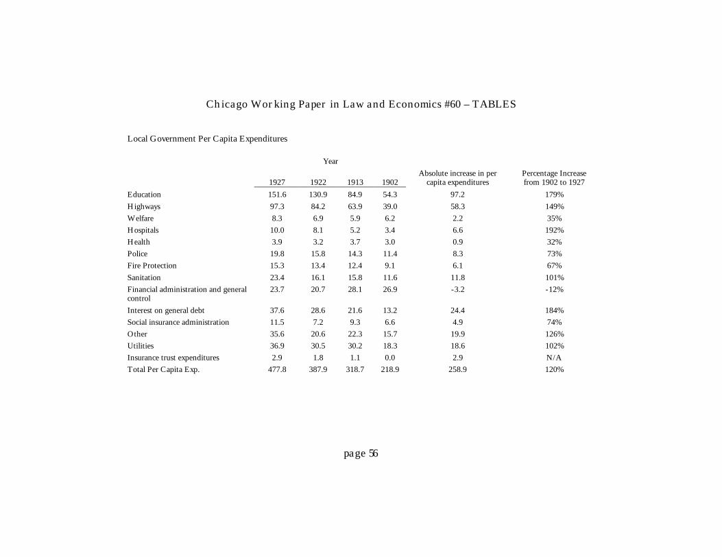
Chicago Working Paper in Law and Economics #60 – TABLES
page 56
Local Government Per Capita Expenditures
Year
1927 1922 1913 1902Absolute increase in per
capita expendituresPercentage Increasefrom 1902 to 1927
Education 151.6 130.9 84.9 54.3 97.2 179%Highways 97.3 84.2 63.9 39.0 58.3 149%Welfare 8.3 6.9 5.9 6.2 2.2 35%Hospitals 10.0 8.1 5.2 3.4 6.6 192%Health 3.9 3.2 3.7 3.0 0.9 32%Police 19.8 15.8 14.3 11.4 8.3 73%Fire Protection 15.3 13.4 12.4 9.1 6.1 67%Sanitation 23.4 16.1 15.8 11.6 11.8 101%Financial administration and generalcontrol
23.7 20.7 28.1 26.9 -3.2 -12%
Interest on general debt 37.6 28.6 21.6 13.2 24.4 184%Social insurance administration 11.5 7.2 9.3 6.6 4.9 74%Other 35.6 20.6 22.3 15.7 19.9 126%Utilities 36.9 30.5 30.2 18.3 18.6 102%Insurance trust expenditures 2.9 1.8 1.1 0.0 2.9 N/ATotal Per Capita Exp. 477.8 387.9 318.7 218.9 258.9 120%

Chicago Working Paper in Law and Economics #60 – TABLES
page 57
Table 6Voting by Members of the U.S. House of Representatives and the Senate:
Additional Turnout and Dummy Variable Specifications(All the Other Variables Controlled for in Table 3 are included here,
though they are not reported. Absolute t-statistics in parentheses)
Voting By Members of theU.S. House of Representatives
Voting ByMembers of the Senate
A. Additional Turnout Specification
Additional Turnout Due to Female Suffrage -.6305(3.385)
-1.4514(5.429)
Additional Turnout Due to Poll Tax 0.9974(4.634)
1.5621(5.023)
Literacy Test -.0217(0.899)
-0.0099(0.285)
Secret Ballot 0.0583(2.143)
0.0200(0.510)
Fixed State EffectsFixed Year Effects
YESYES
YESYES
Adjusted R-Square 0.6757 0.6614
Root Mean Squared Error 0.1982 0.2862
F-Statistic 35.44 33.289
Number of Observations 1587 1587
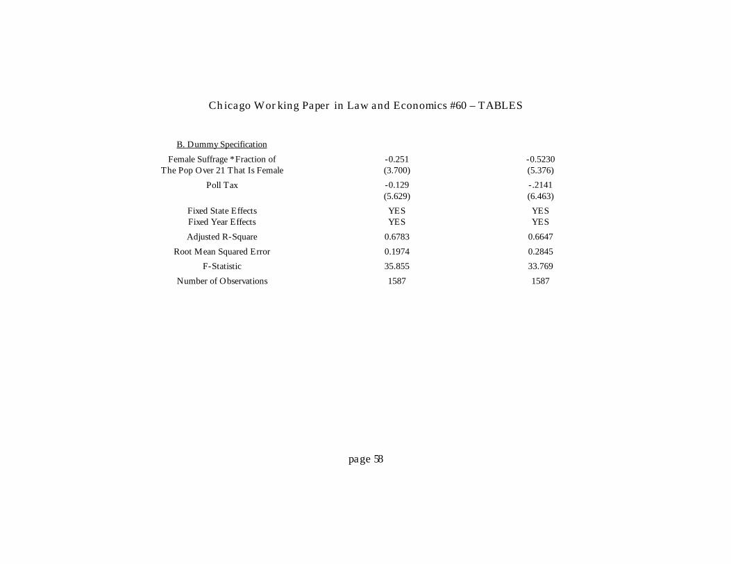
Chicago Working Paper in Law and Economics #60 – TABLES
page 58
B. Dummy Specification
Female Suffrage * Fraction ofThe Pop Over 21 That Is Female
-0.251(3.700)
-0.5230(5.376)
Poll Tax -0.129(5.629)
-.2141(6.463)
Fixed State EffectsFixed Year Effects
YESYES
YESYES
Adjusted R-Square 0.6783 0.6647
Root Mean Squared Error 0.1974 0.2845
F-Statistic 35.855 33.769
Number of Observations 1587 1587

Chicago Working Paper in Law and Economics #60 – TABLES
page 59
Table 7Giving Women the Right to Vote and the Probability that a State will Support
Prohibition or Law Limiting Hours of Employment in Manufacturing for Adult Women
(Estimates are made using probit estimation procedures. All the Other Variables Controlled for in Table 3 areincluded here, though they are not reported. Chi Square statistics are in parentheses)
Prohibition LegislationYes = 1 / No = 0
First Law ImplementingMaximum Hours Legislation
Yes = 1 / No = 0
A. Additional Turnout Specification
Additional Turnout Due to Female Suffrage 140.25(90.37)
-0.5976(0.063)
Additional Turnout Due to Poll Tax -192.01(73.75)
22.796(20.37)
Literacy Test 0.184(0.228)
-0.560(0.614)
Secret Ballot 0.013(0.0017)
-0.4239(1.254)
Fixed State EffectsYear Trend and Trend Squared
YESYES
YESYES
Log Likelihood for Normal Number of Observations -285.612379
-199.183339
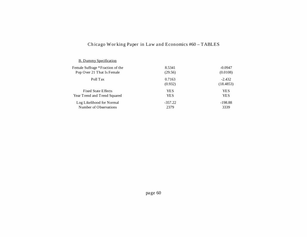
Chicago Working Paper in Law and Economics #60 – TABLES
page 60
B. Dummy Specification
Female Suffrage * Fraction of thePop Over 21 That Is Female
8.5341(29.56)
-0.0947(0.0108)
Poll Tax 0.7163(0.932)
-2.432(18.4853)
Fixed State EffectsYear Trend and Trend Squared
YESYES
YESYES
Log Likelihood for NormalNumber of Observations
-357.222379
-198.883339

Chicago Working Paper in Law and Economics #60 – TABLES
page 61
Table 8Divorce Laws:
Length of desertion in years before divorce is allowed, whether alimony is granted pending suit and whether itis just the woman or the man and the woman who may receive it, and whether permanent alimony is granted and
whether it is just the woman or the man and the woman who may receive it
(All the Other Variables Controlled for in Table 3 are included here, though they are not reported. Absolute t-statistics are shown in parentheses. While these estimates use Ordinary Least Squares, when attempts were made to
use probits with the fixed effects we were not able to get the procedures to converge.)
Alimony May Be Granted Pending Suit Permanent Alimony May Be Granted
Length of DesertionRequired for
Divorce in Yrs.
Shall (2) /May (1) / No(0)
Granted to Women (1)or Women & Men (0)
Shall (2) /May (1) / No(0)
Granted to Women (1)or Women & Men (0)
A. Additional TurnoutSpecification
Additional TurnoutDue to Female
Suffrage
.5342(2.591)
-.4095(3.711)
.1243(1.411)
.0786(1.162)
.2290(2.912)
Additional TurnoutDue to Poll Tax
.2540(1.017)
-.3416(2.549)
.2092(1.787)
.0015(0.019)
.1680(1.770)
Literacy Test -.0899(3.294)
-.0858(5.855)
-.0553(-4.250)
.011(1.260)
0.0241(2.353)
Secret Ballot .1240(3.991)
-.0102(0.601)
0.0110(0.712)
-.0195(1.886)
-.0074(0.563)
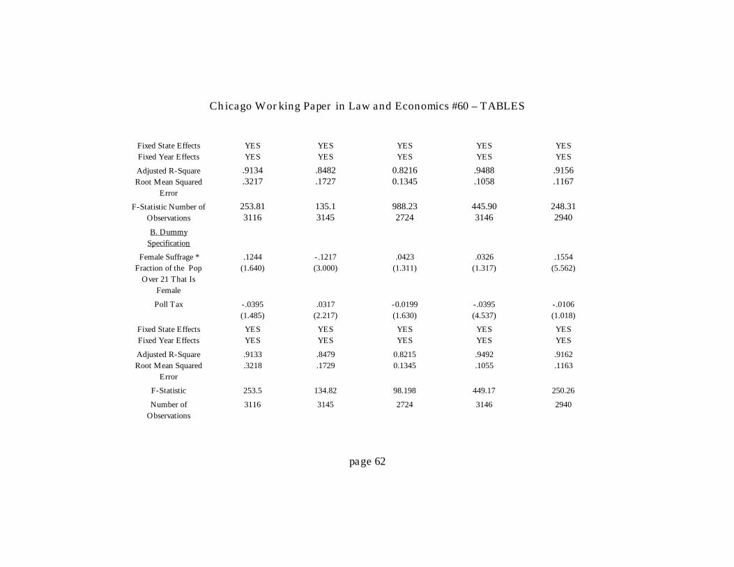
Chicago Working Paper in Law and Economics #60 – TABLES
page 62
Fixed State EffectsFixed Year Effects
YESYES
YESYES
YESYES
YESYES
YESYES
Adjusted R-SquareRoot Mean Squared
Error
.9134
.3217.8482.1727
0.82160.1345
.9488
.1058.9156.1167
F-Statistic Number ofObservations
253.813116
135.13145
988.232724
445.903146
248.312940
B. DummySpecification
Female Suffrage *Fraction of the Pop
Over 21 That IsFemale
.1244(1.640)
-.1217(3.000)
.0423(1.311)
.0326(1.317)
.1554(5.562)
Poll Tax -.0395(1.485)
.0317(2.217)
-0.0199(1.630)
-.0395(4.537)
-.0106(1.018)
Fixed State EffectsFixed Year Effects
YESYES
YESYES
YESYES
YESYES
YESYES
Adjusted R-SquareRoot Mean Squared
Error
.9133
.3218.8479.1729
0.82150.1345
.9492
.1055.9162.1163
F-Statistic 253.5 134.82 98.198 449.17 250.26
Number ofObservations
3116 3145 2724 3146 2940

Chicago Working Paper in Law and Economics #60 – TABLES
page 63
Table 9: Do States that Adopted These Laws Voluntarily Differ fromThose that Had Them Imposed upon Them by the 19th Amendment?
(All the other variables controlled for in Table 3 are included here,though they are not reported. Absolute t-statistics in parentheses)
Endogenous Variables
House Voting Senate Voting Total State Revenue Total State Expenditures
A. Additional Turnout Specification
Additional Turnout Due to FemaleSuffrage Adopted Voluntarily
-0.6574(3.472)
-1.577(5.814)
0.3965(1.736)
0.514789(1.632)
Additional Turnout Due to FemaleSuffrage Adopted under 19th
-.5383(2.452)
-1.0203(3.238)
1.7636(5.147)
1.7581(4.720)
Additional Turnout Due to Poll Tax .9814(4.539)
1.4898(4.779)
-.0806(0.201)
-.4541(1.059)
Literacy Test -.0228(0.943)
-.01555(.444)
.1943(4.148)
.0505(0.986)
Secret Ballot 0.0561(2.048)
.0093(.236)
.02133(0.345)
-.0344(0.600)
Fixed State EffectsFixed Year Effects
YESYES
YESYES
YESYES
YESYES
Adjusted R-Square .6756 .6627 .8416 .8189
Root Mean Squared Error .1982 .2857 .3732 .40859

Chicago Working Paper in Law and Economics #60 – TABLES
page 64
F-Statistic 35.076 33.138 78.252 68.827
Number Of Observations 1587 1587 1817 1875
B. Dummy Specification
Female Suffrage * Fraction of the PopOver 21 That Is Female Adopted
Suffrage Voluntarily
-.252(3.646)
-.557(5.625)
0.1215(1.681)
0.1421(1.611)
Female Suffrage * Fraction of the PopOver 21 That Is Female Adopted
Suffrage Under 19th
-.2466(2.845)
-.3824(3.068)
.7135(5.129)
0.6686(4.457)
Poll Tax -.129(5.541)
-.2047(6.109)
-.082(1.969)
-.0743(1.655)
Fixed State EffectsFixed Year Effects
YESYES
YESYES
YESYES
YESYES
Adjusted R-Square .6781 .6652 .8421 .8189
Root Mean Squared Error .1975 .2846 .3727 .4086
F-Statistic 35.461 33.51 78.51 68.835
Number Of Observations 1587 1587 1817 1875

Chicago Working Paper in Law and Economics #60 – TABLES
page 65
Table 10Sample Means and Standard Deviations for Data Examining Why Women Vote So Differently
Mean Standard Dev. Number of Obs.
Percent of State and Local Government Employees Who are Women .435 .035 392
Gender Gap in Gubernatorial Races where the gap is: (Percent of theFemale Vote for the Democrat - Percent of the Female Vote for theRepublican) - (Percent of the Male Vote for the Democrat - Percent ofthe Male Vote for the Republican) 9.7 9.6 92
Gender Gap in Senate Races 11.1 9.2 139
Gender Gap in Presidential Races 11.7 8.9 126
Gender of Democrat Gubernatorial Candidate (Male =1, Female = 0) .84 .37 92
Gender of Republican Gubernatorial Candidate (Male =1, Female = 0) .90 .30 92
Single Mothers Raising Children Divided by the Number of MarriedCouples with Children (U.S. Census Department) — 1990 only .257 .127 51
Percent of Population Without Health Insurance (U.S. CensusDepartment) — 1994 only 13.8 3.72 51
Unemployment Rate (Statistical Abstract)— 1990 only— 1994 only
5.365.63
1.121.2
5050
Real Per Capita Income in 1983 dollars (Statistical Abstract)— 1990 only— 1994 only
13,67514,244
2,2582,071
5150

Chicago Working Paper in Law and Economics #60 – TABLES
page 66
Table 11Do Women Vote Differently Because of Higher Possible Employment Rates By Government?
(The numbers reported in parentheses are absolute t-statistics)
Endogenous Variable: Gender Gap in Gubernatorial Races(Percent of the Female Vote for the Democrat - Percent of the
Female Vote for the Republican) - (Percent of the Male Vote forthe Democrat - Percent of the Male Vote for the Republican)
(1) (2) (3) (4) (5)
Percent of State and Local GovernmentEmployees Who are Women
52.2(0.529)
41.4(1.250)
-916.36(2.566)
65.54(1.477)
65.3(0.533)
Gender Gap in Senate Races .668(3.448)
.6106(5.685)
. . . . . . . . .
Gender Gap in Presidential Races . . . . . . 1.21(4.317)
.176(1.122)
. . .
Gender of Democrat Gubernatorial Candidate(Male =1, Female = 0)
-17.66(3.743)
-13.3(4.772)
-30.9(4.992)
-5.78(1.722)
-6.81(1.355)
Gender of Republican Gubernatorial Candidate(Male =1, Female = 0)
2.77(0.595)
-2.8(0.628)
11.1(3.610)
2.99(0.878)
1.003(0.216)
Fixed State EffectsFixed Year Effects
YESYES
NONO
YESYES
NONO
YESYES
Adjusted R-Square .8001 .4649 .9110 .2771 .3590
F-Statistic 5.75 12.08 11.92 2.53 1.92
Number Of Observations 52 52 17 17 80
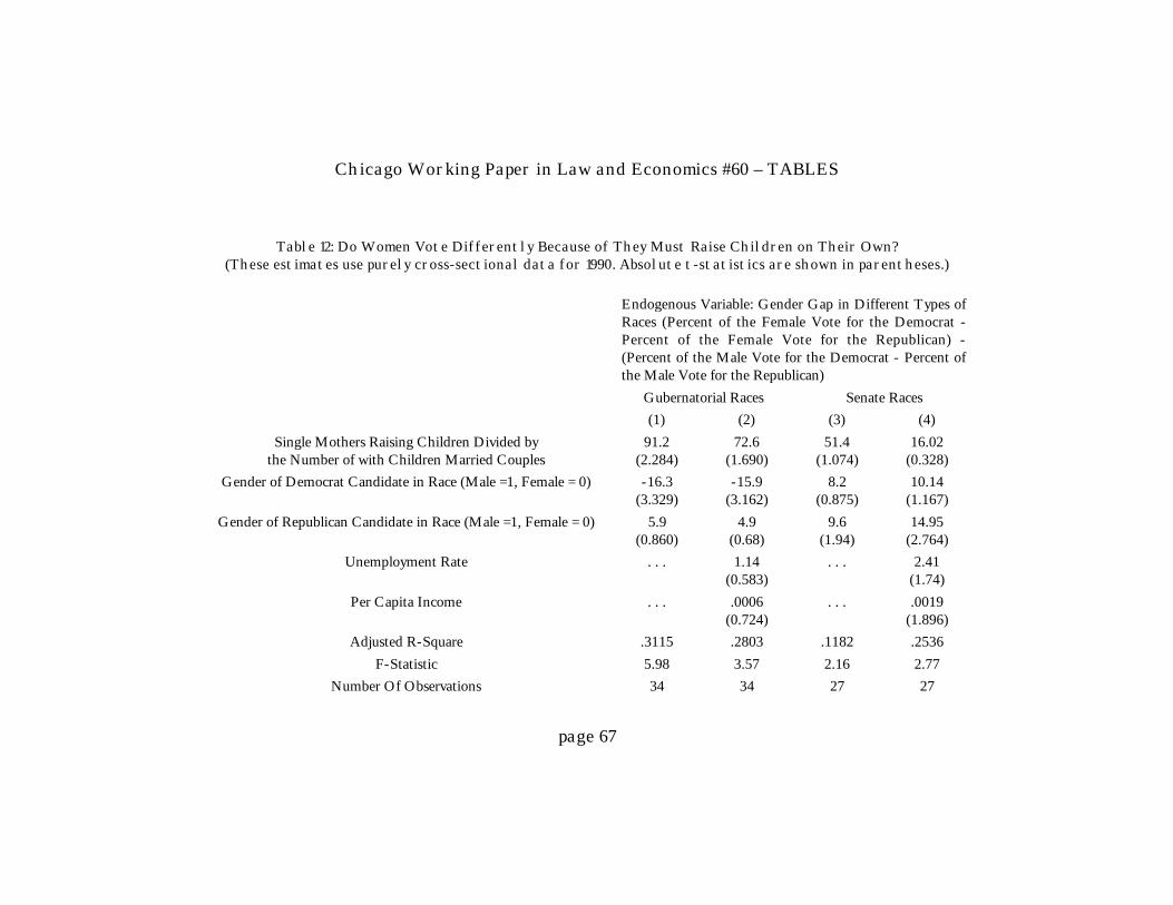
Chicago Working Paper in Law and Economics #60 – TABLES
page 67
Table 12: Do Women Vote Differently Because of They Must Raise Children on Their Own?(These estimates use purely cross-sectional data for 1990. Absolute t-statistics are shown in parentheses.)
Endogenous Variable: Gender Gap in Different Types ofRaces (Percent of the Female Vote for the Democrat -Percent of the Female Vote for the Republican) -(Percent of the Male Vote for the Democrat - Percent ofthe Male Vote for the Republican)
Gubernatorial Races Senate Races
(1) (2) (3) (4)
Single Mothers Raising Children Divided bythe Number of with Children Married Couples
91.2(2.284)
72.6(1.690)
51.4(1.074)
16.02(0.328)
Gender of Democrat Candidate in Race (Male =1, Female = 0) -16.3(3.329)
-15.9(3.162)
8.2(0.875)
10.14(1.167)
Gender of Republican Candidate in Race (Male =1, Female = 0) 5.9(0.860)
4.9(0.68)
9.6(1.94)
14.95(2.764)
Unemployment Rate . . . 1.14(0.583)
. . . 2.41(1.74)
Per Capita Income . . . .0006(0.724)
. . . .0019(1.896)
Adjusted R-Square .3115 .2803 .1182 .2536
F-Statistic 5.98 3.57 2.16 2.77
Number Of Observations 34 34 27 27

Chicago Working Paper in Law and Economics #60 – TABLES
page 68
Table 13General Election Exit Polls Means and Standard Deviations for Reported Variables
1988 General Election Exit Poll 1996 General Election Exit Poll
MeanStandardDeviation Observations Mean
StandardDeviation Observations
Ideology 2.11 .72 31,913 2.099 .717 15,205
Vote for Democrat for President .47 .50 34,245 .51 .50 16,637
Vote for Republican for President .48 .50 34,245 .37 .48 16,637
Identify Self as Democrat .38 .49 34,245 .39 .488 16,637
Identify Self as Republican .31 .46 34,245 .30 .46 16,637
Abortion Matters the Most *Democrat Party Dummy
.03 .17 34,245
Abortion Matters the Most *Republican Party Dummy
.03 .16 34,245
Abortion (Legal, Mostly Legal,Mostly Illegal, Illegal)
2.22 .97 3,822
Taxes Matter the Most *Democrat
.05 .21 34,245
Taxes Matter the Most *Republican
.06 .23 34,245 .03 .17 16,637
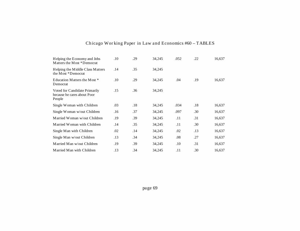
Chicago Working Paper in Law and Economics #60 – TABLES
page 69
Helping the Economy and JobsMatters the Most * Democrat
.10 .29 34,245 .052 .22 16,637
Helping the Middle Class Mattersthe Most * Democrat
.14 .35 34,245
Education Matters the Most *Democrat
.10 .29 34,245 .04 .19 16,637
Voted for Candidate Primarilybecause he cares about PoorPeople
.15 .36 34,245
Single Woman with Children .03 .18 34,245 .034 .18 16,637
Single Woman w/out Children .16 .37 34,245 .097 .30 16,637
Married Woman w/out Children .19 .39 34,245 .11 .31 16,637
Married Woman with Children .14 .35 34,245 .11 .30 16,637
Single Man with Children .02 .14 34,245 .02 .13 16,637
Single Man w/out Children .13 .34 34,245 .08 .27 16,637
Married Man w/out Children .19 .39 34,245 .10 .31 16,637
Married Man with Children .13 .34 34,245 .11 .30 16,637

Chicago Working Paper in Law and Economics #60 – TABLES
page 70
Table 14The Effect of Martial Status and the Presence of Children on People’s Ideology, Voting, and Party Identification
(The missing category is married men without children, so all the categories are interpreted as deviations from what that groupbelieves. While not reported each regression controls for income, type of employment, education, religion, age, race, sex, howurban or rural was the area they lived in, whether they and/or anyone in their family were union members, as well as whatstate they lived in. The regressions for 1988 also control for the type of employment. Absolute t-statistics and Chi-square values are shown in parentheses.)
Ideology* Presidential Vote†Self Identified
DemocratSelf Identified
Republican Taxes§ Education# Poverty**
1988 1996 Dukakis1988
Clinton1996
Dole1996
1988 1996 1988 1996 Dem.1988
Rep.1988
Rep. 1996 1996 1988
Single Womanwith Children
-.22(8.798)
-.12(1.985)
.76(9.437)
.92(4.362)
-1.04(-4.217)
.46(5.996)
.55(2.820)
-.66(7.003)
-.82(3.313)
.32(2.181)
-.58(3.076)
-1.02(2.041)
.68(2.082)
.54(5.920)
Single Womanw/out Children
-.20(13.14)
-.12(2.816)
.50(10.67)
.65(4.681)
-.48(3.253)
.31(6.723)
.39(2.856)
-.23(4.611)
-.26(1.686)
.22(2.195)
-.25(2.737)
-.73(2.857)
.46(1.753)
.21(3.375)
Married Womanw/out Children
-.12(8.837)
-.09(2.219)
.38(9.125)
.40(3.135)
-.22(1.691)
.25(5.123)
.30(2.332)
-.12(2.828)
-.17(1.256)
.29(2.545)
-.16(2.048)
-.56(1.992)
.42(1.637)
.36(6.360)
Married Womanwith Children
-.11(6.665)
-.08(1.859)
.34(6.837)
.32(2.356)
-.23(1.634)
.24(5.621)
.26(1.923)
-.18(3.497)
-.16(1.098)
.20(2.101)
-.25(2.565)
-.41(1.778)
.41(1.618)
.28(4.029)
Single Man withChildren
-.05(1.692)
-.08(1.017)
.20(2.137)
-.005(0.018)
-.05(0.171)
.03(0.351)
.28(1.097)
-.25(2.315)
-.15(0.511)
-.07(0.345)
-.14(0.691)
-.14(0.299)
.71(1.845)
.19(1.569)
Single Manw/out Children
-.06(1.991)
.005(0.112)
.09(1.858)
-.014(0.094)
-.09(0.593)
-.07(1.305)
-.16(1.051)
-.0007(0.013)
-.08(0.518)
-.16(1.286)
-.14(1.821)
-.16(0.952)
-.35(1.075)
.09(1.393)

Chicago Working Paper in Law and Economics #60 – TABLES
page 71
Married Manwith Children
.02(1.392)
.156(3.636)
-.12(2.501)
-.32(2.354)
.34(2.438)
-.13(2.710)
-.21(1.521)
.07(1.557)
.25(1.722)
-.15(1.249)
-.05(0.625)
.09(0.380)
-.07(0.253)
.13(1.88)
State FixedEffects
YES YES YES YES YES YES YES YES YES YES YES YES YES YES
LogLikelihood =
-18374 -2014.7 -1874 -18179 -2029.4 -17020 -1796 -5062.7 -6602 -1693 -758.7 -11721
adj-R2 .0965 .1169
Number ofObservation
28,768 3341 29,453 3,385 3,385 29,453 3,385 29,453 3,385 29,453 29,453 3,365 3,365 29,453
Chi-square 4042 661.4 713.5 3171.8 538.4 3144 600.6 859.4 453.5 385.5 209.4 1206.6
F-statistic 48.28 6.53
* (Liberal=1, Moderate=2, and Conservative=3)† (Only Dukakis is reported for 1988 because there were no significant third party candidates).§ (Endogenous variable is Party Dummy * Taxes Matter the Most. Only nine-tenths of one percent of the respondents were Democrats who listed taxes as their greatest concern in1996. Because of this the regressions were unable to distinguish between the different categories of women and men.# (Endog. variable is Democrat Dummy * Education Matters the Most)** Did the factor that “He Cares About Poor People” Matter Most in Deciding How One Voted (Yes=1, No=0)
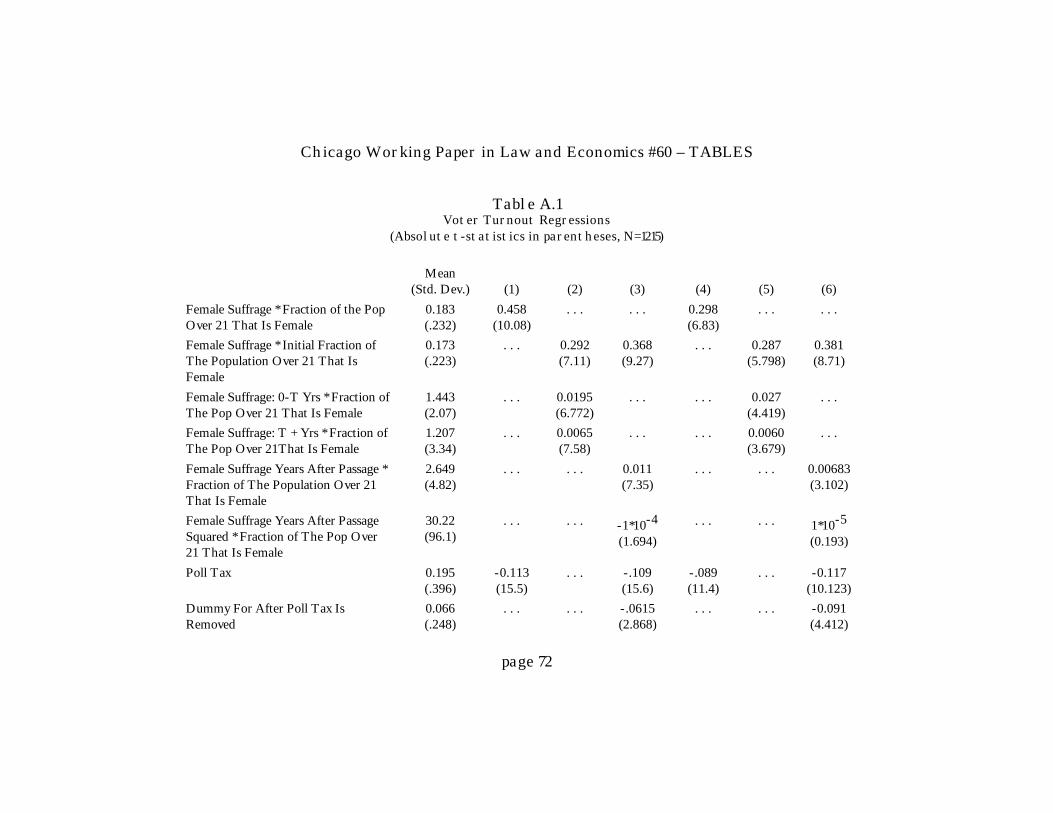
Chicago Working Paper in Law and Economics #60 – TABLES
page 72
Table A.1Voter Turnout Regressions
(Absolute t-statistics in parentheses, N=1215)
Mean(Std. Dev.) (1) (2) (3) (4) (5) (6)
Female Suffrage * Fraction of the PopOver 21 That Is Female
0.183(.232)
0.458(10.08)
. . . . . . 0.298(6.83)
. . . . . .
Female Suffrage * Initial Fraction ofThe Population Over 21 That IsFemale
0.173(.223)
. . . 0.292(7.11)
0.368(9.27)
. . . 0.287(5.798)
0.381(8.71)
Female Suffrage: 0-T Yrs * Fraction ofThe Pop Over 21 That Is Female
1.443(2.07)
. . . 0.0195(6.772)
. . . . . . 0.027(4.419)
. . .
Female Suffrage: T + Yrs * Fraction ofThe Pop Over 21That Is Female
1.207(3.34)
. . . 0.0065(7.58)
. . . . . . 0.0060(3.679)
. . .
Female Suffrage Years After Passage *Fraction of The Population Over 21That Is Female
2.649(4.82)
. . . . . . 0.011(7.35)
. . . . . . 0.00683(3.102)
Female Suffrage Years After PassageSquared * Fraction of The Pop Over21 That Is Female
30.22(96.1)
. . . . . . -1*10-4
(1.694)
. . . . . . 1*10-5
(0.193)
Poll Tax 0.195(.396)
-0.113(15.5)
. . . -.109(15.6)
-.089(11.4)
. . . -0.117(10.123)
Dummy For After Poll Tax IsRemoved
0.066(.248)
. . . . . . -.0615(2.868)
. . . . . . -0.091(4.412)

Chicago Working Paper in Law and Economics #60 – TABLES
page 73
Poll Tax Linger: _,T . . . . . . -.113(16.3)
. . . . . . -0.127(13.71)
. . .
Poll Tax Years After Removed 1.394(6.436)
. . . . . . 0.0038(1.809)
. . . . . . 0.0023(1.437)
Poll Tax Years After RemovedSquared
43.335(248.2)
. . . . . . 1*10-5
(0.24)
. . . . . . .000047(1.476)
Dummy Variable For A Literacy Test 0.239(.426)
-0.040(6.462)
-0.037(6.07)
-0.035(5.771)
0.0034(0.420)
0.010(1.29)
0.0144(1.806)
Dummy Variable For A Secret Ballot 0.681(.466)
-0.040(6.13)
-0.029(4.72)
-0.033(5.32)
-.030(3.49)
-.021(2.57)
-.020(2.448)
Dummy Variable For A PresidentialElection
0.470(.499)
0.072(15.9)
0.069(16.5)
0.069(16.5)
0.047(5.05)
0.046(5.13)
0.050(5.54)
Dummy Variable For A SenateElection
0.297(.457)
-0.0043(0.68)
-0.0019(0.32)
-0.0037(0.62)
-5*10-4
(0.10)
.0009(0.18)
0.00025(0.049)
Winning Governor Vote Share 0.582(.137)
-0.410(16.7)
-0.410(17.8)
-0.401(17.48)
-.306(13.8)
-.293(13.52)
-.293(13.6)
Log Population 7.070(1.03)
-0.0060(1.925)
-0.0095(3.209)
-0.0056(1.815)
-.205(2.41)
-.139(1.646)
-.099(1.176)
Fraction of The Pop. Age 65 AndOlder
0.045(.019)
1.549(8.11)
1.11(6.065)
1.210(6.573)
-.364(1.013)
-.455(1.292)
-.583(1.646)
Fraction of The Pop. Over Age 10That Are Illiterate
0.097(.117)
-0.055(1.439)
-0.0039(0.11)
0.0062(0.172)
0.433(8.57)
.286(5.396)
.2929(5.310)
Relative Manuf Wage -0.068(.905)
0.054(11.3)
0.056(12.4)
0.055(12.1)
0.020(2.65)
.019(2.512)
.0206(2.800)

Chicago Working Paper in Law and Economics #60 – TABLES
page 74
Real Manuf Wage 2096.3(1189)
-7*10-6
(2.710)-7*10-6
(2.81)-3*10-6
(1.315)-8*10-6
(0.72)-7*10-6
(0.666)-1*10-5
(1.013)
Female Workers 0.283(.114)
0.032(0.842)
0.023(0.63)
0.012(0.340)
0.461(7.57)
.497(8.47)
.521(8.752)
Female Workers * Female Suffrage 0.113(.150)
-0.187(2.794)
-0.146(2.49)
-0.219(3.66)
-.070(1.15)
-.132(2.172)
-.201(3.314)
Rural 0.633(.221)
-0.269(4.143)
-0.15(2.416)
-0.0039(0.06)
0.154(1.77)
.121(1.422)
0.119(1.411)
Rural2 0.449(.250)
0.286(5.458)
0.23(4.70)
0.122(2.265)
0.109(1.61)
0.104(1.595)
0.059(0.899)
Log Density 3.427(1.43)
-0.0049(1.290)
0.007(1.886)
0.0062(1.687)
0.198(2.288)
0.125(1.435)
0.081(0.941)
Fraction of the Pop. That Is ForeignBorn
0.134(.099)
-0.380(9.10)
-0.268(6.559)
-0.252(6.182)
-.482(7.47)
-.509(8.11)
-.489(7.798)
Intercept 0.670(15.5)
0.596(14.8)
0.51(11.79)
1.10(2.81)
1.06(2.659)
.99(2.50)
Fixed State EffectsFixed Year Effects
NONO
NONO
NONO
YESYES
YESYES
YESYES
Adjusted R-Square 0.7769 0.8040 .8070 .8871 .8933 .8953
Root Mean Squared Error 0.0771 0.0723 .0718 .0549 .0534 .0529
F-Statistic 235.88 250.1 221.69 96.406 100.7 99.83


