Embed Size (px)
Citation preview

Chemo-dynamical Simulations of
the Milky Way
by
Chris Brook
A DissertationPresented in fulfillment of the requirements
for the degree ofDoctor of Philosophy
at Swinburne University Of Technology
March 2004

Abstract
Using a state of the art galaxy formation software package, GCD+, we model the
formation and evolution of galaxies which resemble our own Galaxy, the Milky Way.
The simulations include gravity, gas dynamics, radiative gas cooling, star formation
and stellar evolution, tracing the production of several elements and the subsequent
pollution of the interstellar medium. The simulations are compared with observa-
tions in order to unravel the details of the Milky Way’s formation. Several unresolved
issues regarding the Galaxy’s evolution are specifically addressed. In our first study,
limits are placed on the mass contribution of white dwarfs to the dark matter halo
which envelopes the Milky Way. We obtain this result by comparing the abundances
of carbon and nitrogen produced by a white dwarf-progenitor-dominated halo with
the abundances observed in the present day halo. Our results are inconsistent with
a white dwarf component in the halo >∼ 5 % (by mass), however mass fractions of
∼1-2 % cannot be ruled out. In combination with other studies, this result sug-
gests that the dark matter in the Milky Way is probably non-baryonic. The second
component of this thesis probes the dynamical signatures of the formation of the
stellar halo. By tracing the halo stars in our simulation, we identify a group of high-
eccentricity stars that can be traced to now-disrupted satellites that were accreted
by the host galaxy. By comparing the phase space distribution of these stars in our
simulations to observed high-eccentricity stars in the solar neighbourhood, we find
evidence that such a group of stars - a “stellar stream” - exists locally in our own
Galaxy. Our next set of simulations demonstrate the importance of strong energy
feedback from supernova explosions to the regulation of star formation. Strong feed-
back ensures that the building blocks of galaxy formation remain gas-rich at early
epochs. We demonstrate that this process is necessary to reproduce the observed
low mass and low metallicity of the stellar halo of the Milky Way. Our simulated
galaxy is shown to have a thick disk component similar to that observed in the Milky
Way through an abrupt discontinuity in the velocity dispersion-versus-age relation
i

ii
for solar neighbourhood stars. This final study suggests that the thick disk forms in
a chaotic merging period during the Galaxy’s formation. Our thick disk formation
scenario is shown to be consistent with observed properties of the thick disk of the
Milky Way.
Acknowledgements
First and foremost, I thank my supervisors Brad Gibson and Daisuke Kawata.
Brad took me on as a PhD student through email correspondence alone. Weboth took a bit of a risk and from my point of view it could not have worked outbetter. Brad’s enthusiasm and energy are legendary. The faith he shows in hisstudents and postdocs provides confidence, and this has definitely been true in mycase.
Daisuke has been invaluable in helping me attain my PhD. He is always helpful,as well as knowledgeable. I am very lucky to have worked with you Daisuke, andwish you a very successful future, which you no doubt have coming.
It has been great to make two such good freinds in Brad and Daisuke.
Thanks to Chris Flynn for his useful advice during my PhD candidacy. It isalways a great pleasure to work with someone as positive as Chris and he remainsa great inspiration to me. I thank Chris and his wonderful wife Lena for their hos-pitality in my stay in Tuorla, and appreciate the Tuorla Observatory for facilitatingmy visit.
I thank everyone at the Centre for Astrophysics and Supercomputing at Swin-burne University. Matthew Bailes accepted me as a PhD student and I am proudto have been a part of the exciting Centre that he has built up. I further thankMatthew for the financial support that he provided on top of the APA.
Huge gratitude and salutations to Annie Hughes for getting me invovled at thecentre, for her unsurpassed skills as an editor, but primarily for being a great freindover the past eight years.
Thanks to David Barnes, James Murray, Andrew Jamieson and Craig West fortheir assistance with all things computer-related.
Thanks to Paul Bourke for his help in creating fantastic animations of our galaxyformation simulations, as well as his assistance in creating posters for Research Weekand conferences.
iii

iv
I am grateful to the Department of Education and Science for their financialassistance in the form of an Australian Postgraduate Award.
Thanks to Masashi Chiba and Tim Beers for providing the data for figure 4.10.Thank you to Andi Burkert and MPIA in Heidleberg, Gerhard Hensler and KielUniversity for their hospitality and facilitating stays at their institutions.
Many people have made suggestions which have helped improve the studies foundin this thesis, including Gerhard Hensler, Andi Burkert, Amina Helmi, Mike Beasley,Stuart Gill, Vincent Eke, Alice Quillen, Tim Connors and a couple of anonymousreferees.
It has been a pleasure to work with the people at Swinburne, and to make freind-ships which will endure. Cheers to Stuart Gill and his wife Nikki, Mike and Amaya,Steve Ord, Chris T., Yeshe, Sarah and Dave, Ago, Craig and anyone I missed.
The support of Max and Sue Brook of my indulgences has been ever present,and unwavering.
Finally, thanks to Kim Kneipp for her encouragement, her support and her love.

Declaration
This thesis contains no material that has been accepted for the award of any otherdegree or diploma. To the best of my knowledge, this thesis contains no materialpreviously published or written by another author, except where due reference ismade in the text of the thesis. All work presented is primarily that of the author.
Science is a collaborative pursuit, and the studies presented in this thesis arevery much part of a team effort. The collaborators listed below have great experi-ence and knowledge, and were all integral in obtaining the presented results.
Chapter 3 was previously published as C. B. Brook, D. Kawata, B. K. Gibson, 2003,“Simulating a white dwarf dominated Galactic halo”, MNRAS 343 913.
Chapter 4 was previously published as C. B. Brook, D. Kawata, B. K. Gibson, &Flynn C. 2003, “Galactic Halo Stars in Phase Space: A Hint of Satellite Accretion?”,MNRAS 585 L125.
Chapter 5 was previously published as C. B. Brook, D. Kawata, B. K. Gibson, &Flynn C. 2004, “Stellar Halo Constraints on Simulated Late Type Galaxies ”, MN-RAS 349 52.The results section has been expanded slightly to include two additional satellitedisruptions events.
Chapter 6 has been submitted to ApJ. as C. B. Brook, D. Kawata, B. K. Gibson,& Freeman K. C. “The Emergence of a Thick Disk in a CDM Cosmology”.
Minor alterations have been made to these studies in order to maintain consistencyof style.
Chris Brook
16 March 2004
v
Contents
1 Background 11.1 Introduction . . . . . . . . . . . . . . . . . . . . . . . . . . . . . . . . 11.2 Our Home Galaxy, The Milky Way . . . . . . . . . . . . . . . . . . . 3
1.2.1 The Thin Disk . . . . . . . . . . . . . . . . . . . . . . . . . . 61.2.2 The Thick Disk . . . . . . . . . . . . . . . . . . . . . . . . . . 61.2.3 The Bulge . . . . . . . . . . . . . . . . . . . . . . . . . . . . . 71.2.4 The Stellar Halo . . . . . . . . . . . . . . . . . . . . . . . . . 81.2.5 The Dark Halo . . . . . . . . . . . . . . . . . . . . . . . . . . 10
1.3 Cosmology and Structure Formation . . . . . . . . . . . . . . . . . . 101.4 A Framework for Disk Galaxy Formation . . . . . . . . . . . . . . . . 131.5 Simulating Galaxy Formation . . . . . . . . . . . . . . . . . . . . . . 141.6 Studies in this Thesis . . . . . . . . . . . . . . . . . . . . . . . . . . . 16
1.6.1 Simulating a White Dwarf-dominated Halo . . . . . . . . . . . 161.6.2 High-eccentricity Halo Stars . . . . . . . . . . . . . . . . . . . 171.6.3 Halo Constraints on Simulated Late-type Galaxies . . . . . . . 171.6.4 The Emergence of the Thick Disk in a CDM Universe . . . . . 18
2 GCD+ 192.1 Introduction . . . . . . . . . . . . . . . . . . . . . . . . . . . . . . . . 192.2 Modeling Dark Matter and Stellar Dynamics: The N-Body Method . 202.3 Modeling Gas Dynamics: The SPH Method . . . . . . . . . . . . . . 212.4 Radiative Gas Cooling . . . . . . . . . . . . . . . . . . . . . . . . . . 262.5 Star Formation . . . . . . . . . . . . . . . . . . . . . . . . . . . . . . 272.6 Initial Mass Function . . . . . . . . . . . . . . . . . . . . . . . . . . . 272.7 Feedback . . . . . . . . . . . . . . . . . . . . . . . . . . . . . . . . . . 28
2.7.1 Supernovae . . . . . . . . . . . . . . . . . . . . . . . . . . . . 282.7.2 Heavy Elements . . . . . . . . . . . . . . . . . . . . . . . . . . 292.7.3 Energy Feedback . . . . . . . . . . . . . . . . . . . . . . . . . 31
3 Simulating a White Dwarf dominated Halo 333.1 Introduction . . . . . . . . . . . . . . . . . . . . . . . . . . . . . . . . 333.2 Method . . . . . . . . . . . . . . . . . . . . . . . . . . . . . . . . . . 36
3.2.1 The Code . . . . . . . . . . . . . . . . . . . . . . . . . . . . . 36
vi
CONTENTS vii
3.2.2 The Model . . . . . . . . . . . . . . . . . . . . . . . . . . . . . 433.3 Results . . . . . . . . . . . . . . . . . . . . . . . . . . . . . . . . . . . 45
3.3.1 White Dwarf-dominated Halo . . . . . . . . . . . . . . . . . . 463.3.2 Chemical Constraints . . . . . . . . . . . . . . . . . . . . . . . 49
3.4 Discussion . . . . . . . . . . . . . . . . . . . . . . . . . . . . . . . . . 523.5 Summary . . . . . . . . . . . . . . . . . . . . . . . . . . . . . . . . . 55
4 Halo Stars in Phase Space 574.1 Introduction . . . . . . . . . . . . . . . . . . . . . . . . . . . . . . . . 574.2 The Code and Model . . . . . . . . . . . . . . . . . . . . . . . . . . . 594.3 Simulation Results . . . . . . . . . . . . . . . . . . . . . . . . . . . . 604.4 Phase Space Analysis . . . . . . . . . . . . . . . . . . . . . . . . . . . 654.5 Discussion . . . . . . . . . . . . . . . . . . . . . . . . . . . . . . . . . 69
5 Constraints on Simulated Late-type Galaxies 725.1 Introduction . . . . . . . . . . . . . . . . . . . . . . . . . . . . . . . . 725.2 The Code and Model . . . . . . . . . . . . . . . . . . . . . . . . . . . 745.3 Results . . . . . . . . . . . . . . . . . . . . . . . . . . . . . . . . . . . 765.4 Discussion . . . . . . . . . . . . . . . . . . . . . . . . . . . . . . . . . 88
6 Thick Disk Formation in a CDM Universe 916.1 Introduction . . . . . . . . . . . . . . . . . . . . . . . . . . . . . . . . 916.2 The Code and Model . . . . . . . . . . . . . . . . . . . . . . . . . . . 936.3 Properties of Final Galaxies . . . . . . . . . . . . . . . . . . . . . . . 946.4 Discussion . . . . . . . . . . . . . . . . . . . . . . . . . . . . . . . . . 97
7 Conclusions and Future Directions 100
References 106
Publications 118

List of Figures
1.1 HST images of remote galaxies . . . . . . . . . . . . . . . . . . . . . . 21.2 The Hubble sequence of galaxy classification . . . . . . . . . . . . . . . 41.3 COBE image of the Milky Way . . . . . . . . . . . . . . . . . . . . . . 51.4 Rotation curve of the Milky Way . . . . . . . . . . . . . . . . . . . . . 71.5 Metallicity distributions of Milky Way components . . . . . . . . . . . . 91.6 Structure formation in CDM cosmology . . . . . . . . . . . . . . . . . . 12
2.1 Cooling rates . . . . . . . . . . . . . . . . . . . . . . . . . . . . . . . . 262.2 Chemical yields . . . . . . . . . . . . . . . . . . . . . . . . . . . . . . . 30
3.1 Salpeter vs. Chabrier IMF . . . . . . . . . . . . . . . . . . . . . . . . . 383.2 Carbon & nitrogen to oxygen abundance ratios . . . . . . . . . . . . . . 423.3 Galaxy evolution in the X-Y plane . . . . . . . . . . . . . . . . . . . . . 453.4 Galaxy evolution in the X-Z plane . . . . . . . . . . . . . . . . . . . . . 463.5 Global star formation rates . . . . . . . . . . . . . . . . . . . . . . . . . 473.6 Final simulated galaxy . . . . . . . . . . . . . . . . . . . . . . . . . . . 473.7 Carbon, nitrogen/oxygen vs. metallicity . . . . . . . . . . . . . . . . . . 51
4.1 δ(U −B) vs. eccentricity for Galactic halo stars . . . . . . . . . . . . . 584.2 metallicity vs. eccentricity for Galactic halo stars . . . . . . . . . . . . . 594.3 The evolution of model 1 . . . . . . . . . . . . . . . . . . . . . . . . . 614.4 The evolution of model 2 . . . . . . . . . . . . . . . . . . . . . . . . . 624.5 Eccentricity distribution of halo stars for 2 models . . . . . . . . . . . . 634.6 X-Z plots of the accretion of S1 . . . . . . . . . . . . . . . . . . . . . . 644.7 X-Z plots of the accretion of S2 . . . . . . . . . . . . . . . . . . . . . . 654.8 Eccentricity distribution of satellite debris . . . . . . . . . . . . . . . . . 664.9 Phase space projections of stars from model 1 . . . . . . . . . . . . . . 674.10 Phase space projections of stars from Chiba & Beers . . . . . . . . . . . 68
5.1 Final galaxies for thermal feedback model & adiabatic feedback model . . 755.2 Star formation rates of 2 models . . . . . . . . . . . . . . . . . . . . . 765.3 Halo metallicity distributions of 2 models . . . . . . . . . . . . . . . . . 775.4 The disruption process for TS1, X-Y plane . . . . . . . . . . . . . . . . 795.5 The disruption process for TS1, X-Z plane . . . . . . . . . . . . . . . . 805.6 The disruption process for TS2, X-Y plane . . . . . . . . . . . . . . . . 81
viii

LIST OF FIGURES ix
5.7 The disruption process for TS2, X-Z plane . . . . . . . . . . . . . . . . 825.8 The disruption process for AS1, X-Y plane . . . . . . . . . . . . . . . . 835.9 The disruption process for AS1, X-Z plane . . . . . . . . . . . . . . . . 845.10 The disruption process for AS2, X-Y plane . . . . . . . . . . . . . . . . 855.11 The disruption process for AS2, X-Z plane . . . . . . . . . . . . . . . . 865.12 Total star formation rates of TS1 & AS1 . . . . . . . . . . . . . . . . . 875.13 Total star formation rates of TS2 & AS2 . . . . . . . . . . . . . . . . . 88
6.1 Density plots of simulated galaxy . . . . . . . . . . . . . . . . . . . . . 946.2 Star formation rates . . . . . . . . . . . . . . . . . . . . . . . . . . . . 956.3 Age-velocity dispersion relation for simulation star particles . . . . . . . . 966.4 Evolution of the simulated galaxy . . . . . . . . . . . . . . . . . . . . . 97

List of Tables
3.1 IMF-weighted stellar yields for massive stars . . . . . . . . . . . . . . . 403.2 IMF-weighted stellar yields for low & intermediate mass stars . . . . . . 413.3 The three models . . . . . . . . . . . . . . . . . . . . . . . . . . . . . 443.4 Stellar and white dwarf number densities . . . . . . . . . . . . . . . . . 49
x
“Equipped with his five senses, man explores the Universe around him and calls thisadventure science.”
Edwin Hubble
“It is not worth an intelligent man’s time to be in the majority. By definition,there are already enough people to do that.”
Godfrey H. Hardy
xi

Chapter 1
Background
1.1 Introduction
Galaxies are the major structural components of our Universe, yet their forma-
tion and evolution remain perhaps the outstanding mystery of contemporary astro-
physics. The latest generation of telescopes, including KECK, VLT, Gemini and
HST provide snapshots of galaxies at various redshifts, providing detail to a degree
almost inconceivable little more than a decade ago (figure 1.1), yet the path taken for
galaxies to evolve between these stages is not clear. At the same time, rapid develop-
ment in computational power has allowed researchers to create increasingly detailed
models of the processes of galaxy formation and evolution. Obviously, the galaxy
for which we have the most information is our home galaxy, the Milky Way. We
have unprecedented access to observational data for the stars of our Galaxy, includ-
ing their distances, kinematics (3 dimensional in many cases), ages and exquisite
chemical abundance determinations. This information is being matched with in-
creasingly sophisticated galaxy formation models and simulations, the goal of which
remains the reconstruction of the Milky Way’s formation and subsequent evolution.
It is hoped that this history will provide a blueprint for the evolution of other disk
galaxies, and indeed the impetus for unraveling a general sequence for the forma-
tion of all galaxies. In this thesis, use is made of a state-of-the-art galaxy formation
simulation code, Galactic Chemo-dynamics Plus -(GCD+)-, to simulate disk galaxies
representative of our Milky Way. These simulations are then compared with obser-
vational data in a series of studies, in order to illuminate specific issues related to
the formation of the Milky Way.
1
CHAPTER 1. BACKGROUND 2
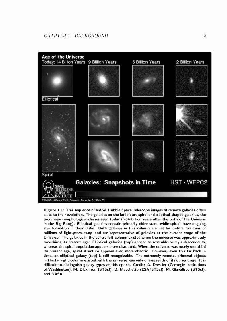
Figure 1.1: This sequence of NASA Hubble Space Telescope images of remote galaxies offersclues to their evolution. The galaxies on the far left are spiral and elliptical-shaped galaxies, thetwo major morphological classes seen today (∼14 billion years after the birth of the Universein the Big Bang). Elliptical galaxies contain primarily older stars, while spirals have ongoingstar formation in their disks. Both galaxies in this column are nearby, only a few tens ofmillions of light-years away, and are representative of galaxies at the current stage of theUniverse. The galaxies in the centre-left column existed when the universe was approximatelytwo-thirds its present age. Elliptical galaxies (top) appear to resemble today’s descendants,whereas the spiral population appears more disrupted. When the universe was nearly one-thirdits present age, spiral structure appears even more chaotic. However, even this far back intime, an elliptical galaxy (top) is still recognizable. The extremely remote, primeval objectsin the far right column existed with the universe was only one-seventh of its current age. It isdifficult to distinguish galaxy types at this epoch. Credit: A. Dressler (Carnegie Institutionsof Washington), M. Dickinson (STScI), D. Macchetto (ESA/STScI), M. Giavalisco (STScI),and NASA

CHAPTER 1. BACKGROUND 3
The remainder of this chapter is used to present a general background to these
studies. A historical context and a cursory examination of the Milky Way’s major
structural components is provided in section 1.2. As theories of galaxy formation
are made within a context of cosmological structure formation, it is necessary to
outline the Big Bang paradigm in section 1.3. A broad picture of current theories of
galaxy formation follows in section 1.4. In section 1.5 galaxy formation models are
introduced, in particular those based upon N-body chemo-dynamical codes. Finally
in section 1.6 we summarise the specific galaxy formation problems investigated in
this thesis.
The chemo-dynamical galaxy evolution code (GCD+), employed here is described
in chapter 2. Chapters 3-6 contain the primary outcomes of this thesis, with each
chapter representing an original study relating to the formation and evolution of the
Galaxy’s dark halo, stellar halo, thin disk and thick disk. A brief note on potential
future work is made in chapter 7.
1.2 Our Home Galaxy, The Milky Way
One of the great sights afforded to mankind is the view of the night sky, highlighted
by the brilliant streak of the Milky Way. It was Galileo who first observed that
the light of the Milky Way emanated from a vast array of stars, showing that the
Milky Way was a stellar system. Subsequent work by, amongst others, Herschel,
Kapteyn and Parsons, set out to discover the structure of the Milky Way, our place
within it, and its relation to other structures such as spiral nebulae. The discovery
of such nebulae, fuzzy objects in the sky that were not planets, comets or stars, is
attributed to Messier in the late 1700s. Herschel (1792-1871) used a large reflecting
telescope to produce a general catalog of these nebulae. By 1920, the two primary
astronomical problems of the day were the size and scale of our Galaxy, and whether
spiral nebulae were extragalactic systems. By 1927, these questions had been settled,
primarily due to observations made by E. Hubble using Cepheid variable stars as
standard candles, setting distance scales to show that spiral nebulae were a great
distance from the Milky Way. In addition, analysis of the kinematics of stars done
by J. H. Oort allowed an estimate of total mass and spatial extent of our Galaxy.
Estimates of the scale of the Milky Way were subsequently improved once the nature
of the absorbing medium in the Galactic Plane was appreciated, for example through
CHAPTER 1. BACKGROUND 4
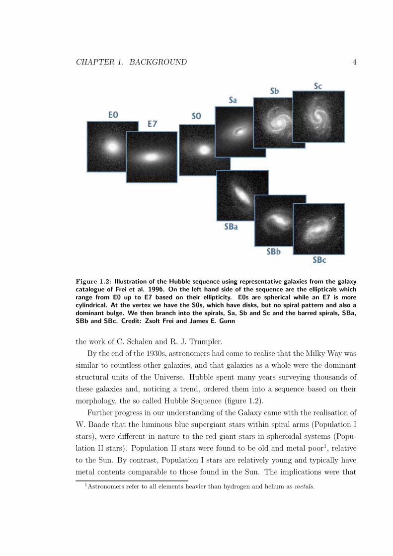
Figure 1.2: Illustration of the Hubble sequence using representative galaxies from the galaxycatalogue of Frei et al. 1996. On the left hand side of the sequence are the ellipticals whichrange from E0 up to E7 based on their ellipticity. E0s are spherical while an E7 is morecylindrical. At the vertex we have the S0s, which have disks, but no spiral pattern and also adominant bulge. We then branch into the spirals, Sa, Sb and Sc and the barred spirals, SBa,SBb and SBc. Credit: Zsolt Frei and James E. Gunn
the work of C. Schalen and R. J. Trumpler.
By the end of the 1930s, astronomers had come to realise that the Milky Way was
similar to countless other galaxies, and that galaxies as a whole were the dominant
structural units of the Universe. Hubble spent many years surveying thousands of
these galaxies and, noticing a trend, ordered them into a sequence based on their
morphology, the so called Hubble Sequence (figure 1.2).
Further progress in our understanding of the Galaxy came with the realisation of
W. Baade that the luminous blue supergiant stars within spiral arms (Population I
stars), were different in nature to the red giant stars in spheroidal systems (Popu-
lation II stars). Population II stars were found to be old and metal poor1, relative
to the Sun. By contrast, Population I stars are relatively young and typically have
metal contents comparable to those found in the Sun. The implications were that
1Astronomers refer to all elements heavier than hydrogen and helium as metals.

CHAPTER 1. BACKGROUND 5
Figure 1.3: This picture was taken by the COBE satellite, and shows the plane of our Galaxyin infrared light. The thin disk is clearly apparent, with stars appearing white and interstellardust appearing red. Credit: E. L. Wright (UCLA), The COBE Project, DIRBE, NASA
the chemical composition of the old stars were likely indicative of primordial mate-
rial formed in the Big Bang, and that heavy elements were made by nucleosynthesis
in the interiors of stars and then recycled into the interstellar medium (ISM). This
work provided insights into stellar evolution, and led to rapid developments in the
fields of stellar structure and evolution, from both a theoretical and observational
perspective. This classification also naturally supported a scenario on which these
two components of the Milky Way formed on different timescales: an old metal-weak
spheroid, and a young, metal rich disk. The concept of characterising distinct stellar
populations by their spatial distribution, kinematic structure, metal content and age
became key in interpreting observations of the Milky Way and other galaxies.
Astronomical work has continued in recent times in establishing details of the
Milky Way’s structure, and characteristics of its constituent stars (figure 1.3). We
know now that our Sun is one of the 200 billion stars in the Milky Way, which
itself has a total mass of approximately 500 billion solar masses (5×10¹¹M) and
diameter 100,000 light years 2. The Milky Way is classified as Hubble type Sb or
Sc (Sbc) (e.g. Hodge 1983), with the possibility of the existence of a central bar
(e.g. Kuijken 1996), which would make it an SBbc, and resides on the periphery
of the great Virgo super cluster. It is widely accepted that our Galaxy has several
2100,000 lyrs '30 kpc, where 1 pc= 3.1×10¹³km
CHAPTER 1. BACKGROUND 6
distinct structural components, and that these components appeared at different
stages in its evolution. The stellar components, the thin disk, the thick disk, and the
spheroid (often broken down again to an inner bulge and outer stellar halo), have
different stellar populations in terms of their kinematic and dynamic properties,
ages, and chemical compositions. The final component of the Galaxy is the dark
halo, presumed to be composed of non-stellar, non-baryonic, matter.
1.2.1 The Thin Disk
The defining stellar component of spiral galaxies, the disk contains stars, star clus-
ters, gas and dust which are confined to the Galaxy’s plane of rotation. The disk
contains ∼90 % of the Milky Way’s baryonic material, approximated by an expo-
nential density distribution with a radial scale length of 4.5 kpc and a scale height
of about 300 pc. The rotation velocity of stars in the disk is relatively constant with
radial distance from the centre (a flat rotation curve, see figure 1.4), with the disk
rotating at about 220 km/s. Thin disk stars are relatively young, with an average
age around 6 Gyrs, with the oldest disk stars around 10 Gyrs old (e.g. Edvards-
son et al. 1993). Age determinations come from the white dwarf cooling sequence,
isochrone estimates for individual evolved stars and open clusters, and radioactive
dating. Disk stars are also metal rich, with a narrow distribution peaking around
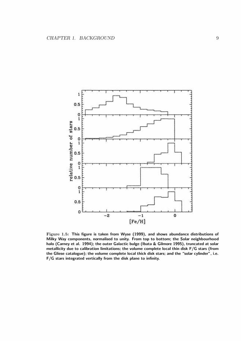
solar metalicity, as shown in the middle panel of figure 1.5. The disk contains sig-
nificant quantities of gas and dust, and is an active site of ongoing star formation,
especially in the spiral arms. Star formation there is believed to be triggered both
by density waves through the spiral arms (Lin & Shu 1964) and by self-sustained
star formation (Talbot & Arnett 1975). Self-sustained star formation occurs when
stellar winds and supernovae explosions from massive stars compress neighbouring
clouds of gas, triggering further star formation. Young hot stars in the disk are
often contained in associations, groups of 10-100 stars which formed recently from
the same nebula, and are moving together through space. Larger, gravitationally
bound open clusters of 100-10,000 stars, also reside in the disk.
1.2.2 The Thick Disk
Using star counts, Gilmore & Reid (1983) showed that the Galaxy has a second disk
component, referred to as the thick disk due to its significantly greater (relative to
the thin disk) vertical scale height, of around 1 kpc (e.g. Phelps et al. 1999). The

CHAPTER 1. BACKGROUND 7
Figure 1.4: A rotation curve for the Milky Way is constructed from measurements of starsand gas in the galactic disk. Figure from Clemens (1985).
thick disk has a surface brightness about 10% that of the thin disk, and the stars
therein are almost exclusively older than 12 Gyrs old (e.g. Gilmore & Wyse 1995).
The bulk of the thick disk stars have metallicities3 in the range −1<[Fe/H]<−0.2,
with a peak near [Fe/H]∼−0.6 (fourth panel of figure 1.5), although there is evidence
for the existence of both metal weak (Chiba & Beers 2000), and metal rich (Feltzing
Bensby & Lundstrom 2003) tails to the metallicity distribution. The thick disk
rotates, lagging the thin disk by about 40 km/s (Gilmore et al. 1989), and is hotter
than the thin disk, with a vertical velocity dispersion of 40-45 km/s (e.g. Chiba
& Beers 2000). The kinematics, age and chemical properties of the thick disk all
support the hypothesis that it is truly a distinct component of the Milky Way, and
not simply a sub-component of the thin disk. Thick disks were not believed to exist
in all disk galaxies (Fry et al. 1999), until the study of 47 edge on disk galaxies by
Dalcanton & Burnstein (2002) provided evidence that thick disks may be ubiquitous.
1.2.3 The Bulge
The central bulge of the Galaxy is a dense swarm of stars, containing approximately
10% of the Galaxy’s mass in a slightly flattened spheroidal distribution with effective
3[Fe/H]≡log(Fe/H)−log(Fe/H), ie the abundance of iron relative to hydrogen of the star,compared to solar ratio, on a log-based ten scale
CHAPTER 1. BACKGROUND 8
radius of ∼2.7 kpc. The bulge stars are generally assumed to be old, an assumption
supported by the presence of RR Lyrae stars, as well as the field colour-magnitude
diagram (Rich 2001). The advent of infrared cameras and adaptive optics techniques
though, has also has revealed the presence of massive stars in the bulge, indicative
of recent star formation. The ISOGAL consortium (van Loon et al. 2003) has
confirmed that the bulge is dominated by old stars (>7 Gyr), but that intermediate
age and young stars (<200 Myr) are also present. The presence of the later is
consistent with the bulges of other spirals, such as M31 (e.g Davies et al. 1991),
M33 (Mighell & Rich 1995), NGC 247 and NGC 2403 (Davidge & Couteau 2002).
The metallicity distribution of the bulge shows significant spread, with a peak near
[Fe/H]∼−0.25 (second panel of figure 1.5). The Milky Way’s bulge appears to be
typical of bulges in late type spirals (Frogel 1990).
1.2.4 The Stellar Halo
The Galactic stellar halo is an approximately 109 M spherical population of stars
and globular clusters, of which there are around 100, and contains little gas, dust or
on-going star formation. The halo has a density distribution which is well approxi-
mated by a power law, ρ ∝ r−3.5. Only ∼1 % of the Milky Way’s stellar component
is found in the halo. The halo has almost no net rotation (Freeman 1987) and is sup-
ported almost entirely by its velocity dispersion. The most kinematically energetic
halo stars have apogalacticons more than 100 kpc from the Galactic centre (Car-
ney et al. 1990). Galactic halo stars are uniformly old, and were probably among
the first galactic objects to form. Dating of halo globular clusters by their main-
sequence turnoff points indicates that they may be as old as 14 Gyrs (e.g. Gratton
et al. 2003). Halo stars are metal poor, with a distribution peak near [Fe/H]∼−1.5
(top panel of figure 1.5), although there does exist a significant range in the halo
MDF. The most metal-poor object known in the Universe is a halo star with an
iron abundance of [Fe/H]∼ −5.4 (Christlieb et al. 2002). The low luminosity of the
stellar halo makes observations of similar extragalactic halos difficult, although a
study by Zibetti et al. (2004) provides some evidence that stellar halos are common
in disk galaxies.
CHAPTER 1. BACKGROUND 9
Figure 1.5: This figure is taken from Wyse (1999), and shows abundance distributions ofMilky Way components, normalised to unity. From top to bottom; the Solar neighbourhoodhalo (Carney et al. 1994); the outer Galactic bulge (Ibata & Gilmore 1995), truncated at solarmetallicity due to calibration limitations; the volume complete local thin disk F/G stars (fromthe Gliese catalogue); the volume complete local thick disk stars; and the “solar cylinder”, i.e.F/G stars integrated vertically from the disk plane to infinity.
CHAPTER 1. BACKGROUND 10
1.2.5 The Dark Halo
The observed rotation of the stars and gas clouds of the Galactic disk suggest that
the visible matter of the Milky Way is surrounded by a dark halo which contains
90% of the Galaxy’s mass, and extends to at least 100 kpc (e.g. Kochanek 1996).
The nature of the dark matter is unknown, and is peraps the greatest contemporary
question facing astrophysics. We will review the evidence for its existence below in
the context of structure formation within current theories of cosmology. The dark
halo of the Milky Way has a density distribution ρ ∼ r−2, and is believed to be
spheroidal (Creze et al. 1998; Ibata et al. 2001; c.f. Helmi 2004).
1.3 Cosmology and Structure Formation
Studying the Coma and Virgo clusters in 1933, Fritz Zwicky found that nearly 10
times as much mass as observed in the form of visible light was needed to keep the
individual galaxies within the cluster gravitationally bound. Zwicky reasoned that
luminous matter made up only a fraction of the matter in the Universe. Scientists
began to explore this discrepancy comprehensively in the 1970’s, and the existence
of dark matter began to be taken seriously. At this time Rubin, Freeman and
Peebles, amongst others, started measuring rotation curves for galaxies, and found
that their orbital speeds remained remarkably constant as radius increased (recall
figure 1.4). The implication was that the there was a significant component of
the Galaxy that we were unable to see. Peebles & Ostriker (1973) found that
numerical simulations of spiral galaxies were unstable when constructed using only
the observed matter distributions; the presence of a dark matter halo enveloping the
visible matter was required. Dark matter has since been invoked to explain a wide
range of observational data, including the motions of stars within dwarf galaxies
(e.g. Aaronson 1987), the motion of globular clusters within elliptical galaxies (e.g.
Huchra & Brodie 1987), X-ray emmisions from clusters (e.g. Mulchaey et al. 1993)
and elliptical galaxies (e.g. Mushotzky et al. 1994; Loewenstein & Mushotzky 2001),
the gravitational lensing of very distant galaxies by foreground clusters (e.g. Tyson
et al 1990), and Big Bang nucleosynthesis (Walker et al. 1991).
Independent of the quest for dark matter, the favoured cosmological framework
for the Universe emerged in the form of the Big Bang model. Edwin Hubble had
shown in 1929 that the more distant a galaxy, the more rapidly it appears to be

CHAPTER 1. BACKGROUND 11
receding, suggesting that the space between galaxies was expanding. George Gamow
argued that this implied that the Universe had emerged from an incredibly dense
and hot state in a cataclysmic event, the so-called “Big Bang”. This hypohesis was
confirmed with the discovery of the predicted cosmic microwave background (CMB)
in 1965 by A. A. Penzias and R. W. Wilson. The Wilkinson Microwave Anisotropy
Probe (WMAP, Spergel et al. 2003) satellite has recently added unprecedented
precision to earlier experiments, such as the Balloon Observations of Millimetric
Extragalactic Radiation and Geophysics (BOOMERANG, de Bernardis et al. 2000)
and the Millimeter Anisotropy Experiment Imaging Array (MAXIMA, Stompor
et al. 2001), in measuring the temperature fluctuations of the CMB imprinted from
the last scattering surface when radiation and matter decoupled.
The accuracy of the current CMB data has resulted in the establishment of what
has been called a “concordance model” of cosmology. We live in a flat Universe, with
total energy density close to the critical density, ρc, or Ω = ρ/ρc ' 1. About 1/3 of
the density is attributed to matter (ΩM = 0.29± 0.07, Spergel el al. 2003), of which
dark matter dominates (ΩDM = 0.243± 0.06), with baryons contributing less than
5 % (ΩB = 0.047± 0.006). The remainder of the critical density is contributed by a
smoothly distributed vacuum energy (ΩΛ = 0.73±0.04), which acts to accelerate the
expansion of the Universe. The existence of this “dark energy” was already suggested
by observations of distant supernovae (Schmidt et al. 1998). The value obtained
from WMAP for the expansion rate of the Universe, the Hubble constant H0, is
consistent with that obtained from earlier HST measurements (H0 = 71.4km/s/kpc;
Gibson et al. 2000).
Most cosmologists favour the cold dark matter (CDM) theory as a description
of how the temperature (i.e. density) perturbations apparent in the CMB become
the seeds for the collapse of matter into overdense regions, and the formation of
structure. The assumption that dark matter is “cold”, or non relativistic, is sup-
ported by the WMAP CMB observations. Warm dark matter may also exist, but
its contribution to the energy density of the Universe is marginal, limited to a few
percent at most (Spergel et al. 2003). In CDM cosmologies, the amplitudes of
density perturbations increase with decreasing scale, with small-scale perturbations
collapsing first. These then merge into larger structures in a process of hierarchical,
or “bottom-up”, structure formation. In order to study how strucure evolves and
forms through these processes, from small fluctuations when the universe was around
300,000 years old to the present day, the non-linear nature of gravity has meant that

CHAPTER 1. BACKGROUND 12
Figure 1.6: A numerical simulation of a ΛCDM Universe. In the top row, we see theformation of large scale structure from the early Universe to the present. The boxes shownare 100 Mpc in size. The statistical properties of the derived distribution at redshift zeroprovide a close match to those derived from large galaxy surveys. By zooming in on a 1 Mpcregion, we see a cluster of galaxies (bottom left), which is seen to resemble the observedcluster C10024+1654 (bottom right). Credit: Alexander Knebe
numerical simulations become crucial. Such simulations have been highly successful
in reproducing many observed structural features of the Universe (see figure 1.6).
The CDM model is consistent with an impressive array of observations, including
the age of the oldest stars (e.g. Chaboyer et al. 1998), the extragalactic distance
scale, as measured by distant Cepheids (e.g. Gibson et al. 2000), the baryonic mass
fraction of galaxy clusters (e.g. White et al. 1993), the abundance of massive galaxy
clusters (e.g. Eke, Cole & Frenk 1996), the shape and amplitude of galaxy clustering
patterns (e.g. Wu, Lahav & Rees 1999), and the magnitude of large-scale coherent
motions of galaxy systems (e.g. Strauss & Willick 1995; Zaroubi et al. 1997).
However, at least two important discrepancies between the predictions of the CDM
paradigm and the observations of galaxies have arisen. First the inner density profile
of virialized CDM halos (Navarro, Frenk & White 1997) is too steep with respect
CHAPTER 1. BACKGROUND 13
to what is inferred from rotation curves of dwarf spiral and low surface brightness
galaxies (e.g. McGaugh & De Block 1998). Second, CDM predicts significantly
greater numbers of dwarf galaxies than are observed in systems such as the Local
Group (Moore et al. 1999; Klypin et al. 1999).
1.4 A Framework for Disk Galaxy Formation
A detailed prescription for the formation of disk galaxies was outlined in Fall &
Efstathiou (1980). In their model, a uniformly rotating, homogeneous protogalactic
cloud of gas begins to collapse when a galaxy de-couples from the Hubble flow
and begins to collapse. This protogalaxy is endowed with angular momentum from
tidal torques driven by surrounding structure (Peebles 1969). It is assumed in their
model that the baryons destined to become the disk receive the same tidal torques
as the dark matter before much disspiation occurs, and thus the two components
initially have the same specific angular momentum. If the collapse is smooth, then
specific angular momentum is conserved and the gas forms a thin, rapidly rotating
disk. This type of model has been successful in explaining several properties of disk
galaxies, including the slope and scatter of the Tully-Fisher relation (Mo, Mao &
White 1998), and the distribution of disk surface brightness profiles (Dalcanton,
Spergel & Summers 1997).
Admittedly a model predicated upon a homogeneous, uniformly rotating proto-
galaxy is at odds with the CDM hierarchical structure formation outlined above,
in which a galaxy is formed through the merger of smaller “building blocks”. The
general scenario of galaxy formation within the cosmological context, as envisioned
by White & Rees (1978), involves extended dark halos of galaxies forming hierar-
chically by gravitational clustering of non-dissipative dark matter. The luminous
components form by a combination of the gravitational clustering and dissipative
collapse. As the baryons cluster and collapse due to gravity, they are shoch-heated
to the virial temperature of the halo, at which point the gas can be fully ionised
and dissipate energy efficiently by means of bremsstrahlung radiation. With hi-
erarchical structure formation, dark matter “building blocks” form first. The gas
then collapses into these building blocks, rather than forming a homogeneous cloud.
Problems with this model are encountered when gas falls to the centre of these
building blocks. When the building blocks subsequently merge, the gas component

CHAPTER 1. BACKGROUND 14
transfers angular momentum to the dark matter. This results in the so called “an-
gular momentum catastrophe” in which simulated spiral galaxies are deficient in
specific anglar momentum when compared with observation (e.g. Navarro, Frenk &
White 1995). In order to reconcile the two models of formation -i.e. (i) creating a
disk galaxy by a collapsing gaseous sphere, and (ii) the general mode of hierarchi-
cal clustyering- White & Rees (1978) suggested it was necessary to include energy
feedback from star formation, preventing gas from collapsing into “building blocks”.
Thus it becomes imperative to include processes such as star formation, energy re-
lease by stellar winds and supernova explosions, and metal enrichment in modeling
the baryonic components of galaxies.
1.5 Simulating Galaxy Formation
One approach which has been used to gain valuable insight into galactic evolution
are semi-analytic galactic chemical evolution codes (Talbot & Arnett 1971; Tinsley
1980). These codes take advantage of the fact that the evolution of individual
stars is reasonably well understood. The basic picture of chemical evolution is
to start with gas of primordial composition and add in an empirical treatment
of star formation (with the mass distribution of newly formed stars -the initial
mass function (IMF)- specified), with chemical enrichment of the ISM traced self-
consistently with each subsequent generation of star birth and death. In addition,
these models may consider input and output of gas from any particular region,
with either primordial or modified composition. Such semi-analytical models have
become increasingly sophisticated, incorporating processes such as enrichment of
the ISM, multiple epochs of infall, differential loss of various elements by galactic
winds, multi-zone models, and time-dependent IMFs (e.g. Matteucci & Francois
1989; Pagel & Tautaisiene 1995; Timmes, Woosely & Weaver 1995; Fenner & Gibson
2003). By tracing the evolution of chemical abundances as they cycle through gas
and stars, these models have been succesful in explaining mean trends in the chemical
properties of galactic systems.
Semi-analytical models (SAMs) of galaxy formation attempt to tie galactic chem-
ical evolution to structure formation. The merger history of a given halo is con-
structed, most commonly by Monte Carlo realisations of the Press-Schechter for-
malism. The gas processes involved in galaxy formation, namely the shock heating

CHAPTER 1. BACKGROUND 15
and radiative cooling of gas, star formation and feedback are followed using a set
of physical laws or, where the physics is poorly understood, phenomenological for-
malisms. The ease of calculations of these models allows large tracts of parameter
space to be explored. White & Frenk (1991) used such models to recover observed
properties of galaxies, including their luminosity functions and Tully-Fisher relation.
Since that pioneering study, SAMs have also become increasingly sophisticated (e.g.
Cole et al. 1994; Cole et al. 2000; Kauffmann 1996; Somerville & Primack 1999).
Numerical models of galaxy formation have one significant advantage over semi-
analytical models by providing a self consistent treatment of kinematics and struc-
tural evolution. Early models incorporating gas dissipative processes can be traced
to Larson (1969), whose axisymmetric models, with self-consistent chemical evolu-
tion included, reproduced several essential properties of elliptical (Larson 1974a,b,
1975) and disk (Larson 1976) galaxies. Carlberg (1984a,b) and Carlberg, Lake &
Norman (1986) improved upon these models, treating gas and star formation pro-
cesses in a phenomenological manner. Various parameters introduced include the
collision rate of gas clouds, the rates of dissipation, star formation efficiency, and
the strength of supernova energy feedback.
Advances in both hardware and software algorithms in the past decade have
dramatically improved the quality of such numerical simulations, increasing the dy-
namical range of the models, as well as the sophistication of physical modeling.
The simulations used in this thesis are predicated on the algorithm developed by
Katz & Gunn (1991), whose code evolves self-gravitating fluids in three dimensions.
Their code -TreeSPH (Hernquist & Katz 1989; Katz, Weinberg & Hernquist 1996)-
is a Lagrangian code which combines smoothed particle hydrodynamics (SPH; Lucy
1977; Gingold & Monaghan 1977) with a hierarchical tree algorithm for computing
gravitational forces (Barnes & Hut 1986). The explicit calculation of the thermody-
namic state of the gas within the TreeSPH algorithm allows radiative cooling to be
included via the use of standard cooling curves, resulting in more realistic modelling
of gas dissipation. Further, TreeSPH allows for the natural inclusion of a treatment
for star formation (Katz 1992) and the subsequent effects of chemical enrichment
(Steinmetz & Muller 1994, 1995).
These early simulations were made within a “semi-cosmological” framework, by
investigating the collapse of an isolated “top-hat” sphere of dark and baryonic mat-
ter which initially follows the Hubble flow. Large scale tidal fields, missing in the
semi-cosmological treatment, are instead incorporated by providing the sphere with

CHAPTER 1. BACKGROUND 16
an initial degree of solid-body rotation, characterised by a dimensionless spin param-
eter, λ (Peebles 1971). Small scale density perturbations were then superimposed
on the sphere, consistent with the CMB and present day structure of the Universe.
Semi-cosmological galaxy evolution models now trace information such as gas tem-
perature and density, stellar age, and various chemical abundances in stars as well as
the ISM. By use of stellar poplulation synthesis models, the photomeric properties
of the simulated galaxies can be investigated and compared with observation (e.g.
Bekki & Shioya 1998; 1999; Steinmetz & Navarro 1999; Mori, Yoshii & Nomoto
1999; Kawata 1999; Koda et al. 2000).
Full cosmological simulations are the most recent development in galaxy forma-
tion codes (e.g. Steinmetz & Navarro 1999; Navarro & Steinmetz 2000; Abadi et al.
2003; Kawata & Gibson 2003b). Here, galaxy sized regions of interest within larger
scale, lower resolution, cosmological simulations are resimulated at higher resolu-
tion, with hydrodynamical gas processes and star formation treatments included.
The background cosmological setting remains at low resolution, but still provides a
realistic halo mass, merging history and tidal forces which ultimately provide angu-
lar momentum and set the collapse redshift. The downside to such simulations is the
extra computational resources required when compared against semi-cosmological
simulations. Semi-cosmological simulations have a further advantage in being read-
ily suited to arbitrary user specified initial conditions. While computational power
has partially eroded the advantages enjoyed by semi-cosmological codes, thier still
superior parameter space coverage abilities made them the method of choice for this
thesis.
1.6 Studies in this Thesis
Each of the components of this thesis is based upon a comparison of the predictions
of our chemo-dynamical semi-cosmological simulations with specific observational
data sets of the Milky Way. The overarching goal of this work is to shed light on
unanswered questions concerning the formation and evolution of our Galaxy.
1.6.1 Simulating a White Dwarf-dominated Halo
Observational evidence has suggested the possibility of a Galactic halo which is
dominated by white dwarfs (WDs). While debate continues concerning the in-
CHAPTER 1. BACKGROUND 17
terpretation of this evidence, it is clear that an IMF biased heavily toward WD
precursors (1 <∼ m/M <∼ 8), at least in the early Universe, would be necessary in
generating such a halo. Within the framework of homogeneous, closed-box models of
Galaxy formation, such biased IMFs lead to an unavoidable overproduction of car-
bon and nitrogen relative to oxygen (as measured against the abundance patterns
in the oldest stars of the Milky Way). Using our three-dimensional Tree N-body
smoothed particle hydrodynamics code, we study the dynamics and chemical evolu-
tion of a galaxy with different IMFs. Both invariant and metallicity-dependent IMFs
are considered. Our variable IMF model invokes a WD-precursor-dominated IMF
for metallicities less than 5% solar (primarily the Galactic halo), and the canon-
ical Salpeter IMF otherwise (primarily the disk). Halo WD density distributions
and C,N/O abundance patterns are presented. While Galactic haloes comprised
of >∼ 5% (by mass) of WDs are not supported by our simulations, mass fractions
of ∼1-2% cannot be ruled out. This conclusion is consistent with the present-day
observational constraints.
1.6.2 High-eccentricity Halo Stars
The present day chemical and dynamical properties of the Milky Way bear the im-
print of the Galaxy’s formation and evolutionary history. One of the most enduring
and critical debates surrounding Galactic evolution is that regarding the competition
between “satellite accretion” and “monolithic collapse”; the apparent strong corre-
lation between orbital eccentricity and metallicity of halo stars was originally used
as supporting evidence for the latter. While modern-day unbiased samples no longer
support the claims for a significant correlation, recent evidence has been presented
by Chiba & Beers (2000) for the existence of a minor population of high-eccentricity
metal-deficient halo stars. It has been suggested that these stars represent the signa-
ture of a rapid (if minor) collapse phase in the Galaxy’s history. Employing velocity-
and integrals of motion-phase space projections of these stars, coupled with a series
of N-body/SPH chemo-dynamical simulations, we suggest an alternative mechanism
for creating such stars may be the recent accretion of a polar orbit dwarf galaxy.
1.6.3 Halo Constraints on Simulated Late-type Galaxies
How do late type spiral galaxies form within the context of a CDM cosmology? The
reconciliation of the models of hierarchical build up of galaxies proposed by White &

CHAPTER 1. BACKGROUND 18
Rees (1978), with the disk galaxy formation model of Fall & Efstathiou (1980), is a
central problem of galaxy formation modeling. It has long been assumed that such a
reconciliation lies with the processes of energy feedback, primarily due to supernova
explosions. Unfortunately these processes have been notoriously difficult to model.
We contrast N-body, smoothed particle hydrodynamical simulations of galaxy for-
mation which employ two different supernova feedback mechanisms. Observed mass
and metallicity distributions of the stellar halos of the Milky Way and M31 provide
constraints on these models. A strong feedback model, incorporating an adiabatic
phase in star burst regions, better reproduces these observational properties than
our comparative thermal feedback model. This demonstrates the importance of en-
ergy feedback in regulating star formation in small systems, which collapse at early
epochs, in the evolution of late-type disk galaxies.
1.6.4 The Emergence of the Thick Disk in a CDM Universe
We simulate a Milky Way like disk galaxy using our chemo-dynamical code, GCD+;
we demonstrate that this disk galaxy has a significant thick disk component. This
is evidenced by the velocity dispersion versus age relation for solar neighbourhood
stars, which clearly shows an abrupt increase in velocity dispersion at a lookback
time of approximately 8 Gyrs, and is in excellent agreement with observation. These
thick disk stars are formed from gas which is accreted onto the Galaxy during a
chaotic period of hierarchical clustering at high redshift. This formation scenario is
shown to be consistent with observations of both the Milky Way and extragalactic
thick disks.

Chapter 2
GCD+
2.1 Introduction
Our Galactic chemo-dynamics software package GCD+ was originally developed by
Kawata (1999). Work on this package is ongoing, as new techniques are developed in
order to better simulate galaxy evolution. Studies employing this software package
form the bulk of the work in this thesis, thus it is necessary to provide the reader with
sufficient background to appreciate its inner workings and capabilities. A number of
enhancements have been made to Kawata’s (1999) original version of GCD+ during
the course of this thesis. These enhancements, as well as the underlying structure
of GCD+ are outlined below.
In GCD+, the dynamics of dark matter and stars are calculated using an N-body
scheme, whilst gas dynamics are modeled using smoothed particle hydrodynamics
(SPH). The code is based on earlier numerical models of galaxy formation which
combine N-body techniques with the SPH method, including Hernquist & Katz
(1989), Navarro & White (1993), Katz et al. (1996) and Steinmetz (1996).
GCD+ is vectorised and parallelized. Parallelization is achieved by use of the MPI
library, so that the code can run efficiently on most platforms from clusters to PCs
to large shared-memory supercomputers. Further details concerning GCD+ can be
found in Kawata (1999, 2000, 2001, hereafter K99, K00, K01) and in Kawata &
Gibson (2003a,b).
19

CHAPTER 2. GCD+ 20
2.2 Modeling Dark Matter and Stellar Dynamics:
The N-Body Method
Physical entities in GCD+ are represented by a large number, N, of point-like particles
which represent the gas, stars and dark matter of the Universe. These particles are
then “tagged” with characteristics corresponding to their physical properties. The
cosmological framework in which GCD+ operates is a standard Cold Dark Matter
(CDM) Universe. Incorporating the gravitational effects of dark matter is perhaps
the most fundamental aspect of structure formation theory. Dark matter is typically
represented within the theory as massive particles that interact with each other and
with baryonic matter particles only through the gravitational force. Computation-
ally this is done via the application of a gravitational N-body algorithm. In addition
to such gravitational forces, gas particles interact with each other via hydrodynam-
ical forces, which are dealt with in the next section.
We employ a gravitational force calculation based upon the hierarchical tree
formalism (Barnes & Hut 1986; Pealzner & Gibbon 1996). The tree algorithm is
computationally efficient, though at the expense of several approximations being
required to describe the gravitational potential. One calculates the multipole mo-
ments of a nested hierarchy of particles in which each particle then interacts with
other elements of the hierarchy, subject to accuracy conditions, in order to calcu-
late gravitational forces. “Clustered” particles well away from from a given single
particle are treated as a single entity with a given multipole expansion of sufficient
accuracy. The ratio of the size of a “cluster” to its distance from the given particle
is compared to a tolerance parameter to determine whether treating that cluster as
a point mass is sufficient, or whether it is necessary to proceed further down the tree
to smaller clusters. As the number of terms in the multipole expansion is typically
small compared with the number of particles in the cluster, a significant gain in
efficiency is realised. Conceptually, the detailed distribution of particles is neglected
when calculating their collective gravitational effect on a given particle, up to a
given level of accuracy, determined by a tolerance parameter. In GCD+, expansion is
made to the quadrupole order with a tolerance parameter θ=0.8.
In order to minimise the effects of two body relaxation, a gravitational softening
length is employed. Specifically, the gravitational force term of the i-th particle is
CHAPTER 2. GCD+ 21
the sum of the contributions from dark matter, star and gas particles
∇iΦ = −G∑
j
mjxij(r2ij + ε2ij)
3/2(2.1)
where rij ≡ |xij|, xij ≡ xi − xj and εij ≡ (εi + εj)/2 is the mean softening length of
the i-th and j-th particles.
2.3 Modeling Gas Dynamics: The SPH Method
Gas dynamics in GCD+ is treated by modeling a collection of particles, using the
smoothed particle hydrodynamics (SPH) method (Lucy 1977; Gingold & Monaghan
1977). These gas particles experience local forces from pressure gradients in addition
to gravitational forces. In SPH the Lagrangian form of the hydrodynamical equa-
tions is used to determine the dynamics of the particles. Local physical conditions
are described by a finite number of neighbour particles in order to mimic a fluid. It
is assumed that the mass density of the fluid is roughly proportional to the particle
mass density. A consequence of this is that susceptibility to local statistical fluctu-
ations in particle numbers must be minimised, which is achieved by introducing the
concept of a “kernel”. GCD+ employs a spherically symmetric spline kernel of the
form
W (r, h) =8
πh3
1− 6(r/h)2 + 6(r/h)3 if 0 ≤ r/h ≤ 1/2,
2[1− (r/h)]3 if 1/2 ≤ r/h ≤ 1,
0 otherwise,
(2.2)
where r is the distance from the particle and h is a particle’s individual smoothing
length, chosen to keep the number of particles within its smoothing length roughly
constant.
We use a smoothing length algorithm based upon that of Thacker et al. (2000),
an improvement upon the original technique used by K99 and K00 (which was
derived from Steinmetz 1996). This variable smoothing length ensures that all
points in the fluid have smoothed quantities computed to the same level of mass
resolution. First, neighbour particles are counted for the i-th particle using the
smoothing kernel,

CHAPTER 2. GCD+ 22
Wnn(r, hi) =
1 if 0 ≤ r/hi ≤ 3/4,
πh3i
8W (4(r/hi − 3/4)) if 3/4 ≤ r/hi ≤ 1,
(2.3)
where r is the distance between the i-th particle and its neighbour, and W(x) is
the spline kernel (equation 2.2). The number of neighbours, Nnb,i is a real number
rather than an integer, alleviating discontinuity in the number of neighbours. Then
the smoothing length, hn+1i , at the time-step n+ 1 is determined by the smoothing
length, hni , and the number of neighbours, Nnnb,i, at the previous time-step n:
hn+1i = hni
1− a+ a
(Ns
Nnnb,i
)1/3 , (2.4)
where Ns = 40 is the desired number of neighbours. This adopted value for Ns
provides acceptable accuracy as demonstrated by one-dimensional shock tube tests.
The variable a changes as a function of the parameter s = (Ns/Nnnb,i)
1/3, as
a =
0.2(1 + s2) if s < 1
0.2(1 + 1/s3) if s ≥ 1(2.5)
Physical parameters pertaining to each particle, such as density, ρ, are then
calculated by
ρi =∑
j
mjW (rij, hij), (2.6)
where hij = (hi + hj)/2 is the pair averaged smoothing length. Euler’s equation is
employed to trace the kinematics of particle i, and takes the form
dvidt
= − 1
ρi∇i(P + Pvisc)−∇iΦi (2.7)
where Φ, P and Pvisc are the gravitational potential, pressure, and the artificial
viscous pressure, respectively. The gravitational force, ∇iΦi, is computed as in
equation (2.1). GCD+ uses the following smoothed estimate of the pressure-gradient
term
1
ρi∇i(P + Pvisc) =
∑
j
(Piρ2i
+Pjρ2j
+Qij
)∇iW (xij, hij), (2.8)

CHAPTER 2. GCD+ 23
where Qij is the artificial viscosity. The artificial viscous pressure term allows for the
presence of shock waves in the flows to be included computationally. Shock fronts
generate energy and transform kinetic energy into internal energy, preferably with
minimum post-shock oscillations to the hydrodynamical variables. The form taken
for the artificial viscosity follows Navarro & Steinmetz (1997),
Qij =
−αvs,ijµij + βµ2ij
ρijif xij · vij < 0,
0 otherwise,
(2.9)
withµij = 0.5hijvij · xij
r2ij + η2
, (2.10)
where vij ≡ vi − vj. The parameters α = 0.5, β = 1.0, controlling the amplitude of
post-shock oscillations, are set to reproduce features of the one-dimensional shock
tube experiment. The parameter η = 0.05hij is introduced to prevent numerical
divergences. A correction is then made in order to reduce the shear component of
the artificial viscosity (see Balsara 1995; Navarro & Steinmetz 1997)
Qij = Qijfi + fj
2, (2.11)
fi =|〈∇ · v〉i|
|〈∇ · v〉i|+ |〈∇ × v〉i|+ 0.0002vs,i/hi(2.12)
where vs is the sound velocity. The velocity divergence and rotation are calculated
by
〈∇ · v〉i = − 1
ρi
∑
j
mjvij · ∇iW (xij, hij), (2.13)
〈∇ × v〉i = − 1
ρi
∑
j
mj[vij,z∇i,yW (xij, hij)− vij,y∇i,zW (xij, hij)], (2.14)
where vij,x ≡ vi,x − vj,x. If the flow is shear-free and compressive, the corrected
viscosity term is identical to the uncorrected term. In the presence of shear flows,
the effect of the correction is to reduce the importance of the viscous term.
The velocity and position of each particle is updated by integrating equation (2.7)
using a leap-frog algorithm with individual time-steps, following Hernquist & Katz

CHAPTER 2. GCD+ 24
(1989) and Makino (1991). The time-step of the i-th particle is chosen to be ∆ti
= min(0.3∆tCFL,i, 0.1∆tf,i), where ∆tCFL is determined by the Courant-Friedrichs-
Lewy condition
∆tCFL,i =0.5hi
vs,i + 1.2(αvs,i + βmaxj |µij|), (2.15)
and ∆ti is determined by the requirement that the force should not change signifi-
cantly from one time-step to the next. This is achieved by
∆tf,i =
√hi2
∣∣∣∣dvidt
∣∣∣∣−1
. (2.16)
A lower limit for the smoothing length is set to be hmin = ε/2. For collisionless dark
matter and star particles, the time-step is determined by
∆t = min[0.16(ε/v), 0.4(ε/|dv/dt|1/2]. (2.17)
The leap-frog method then involves integrating the position and velocity in the
following manner:
vn+1/2 = vn + 0.5
(dv
dt(xn, vn, ...)
)n∆tn→n+1, (2.18)
xn+1 = xn + vn+1/2∆tn→n+1, (2.19)
vn+1 = vn+1/2 + 0.5
(dv
dt(xn, vn, ...)
)n∆tn→n+1, (2.20)
vn+1 = vn+1/2 + 0.5
(dv
dt(xn+1, vn+1, ...)
)n+1
∆tn→n+1, (2.21)
where ∆tn→n+1 represents a time interval between n and n+ 1 steps.
The smoothed form of the thermal energy equation used in GCD+ to determine
the evolution of the internal energy, ui is
duidt
=Piρi
∑
j
mjvij ·∇iW (xij, hij)+1
2
∑
j
mjQijvij ·∇iW (xij, hij)−Λi
ρi+Hi, (2.22)

CHAPTER 2. GCD+ 25
where Λρ and H are the cooling rate and heating rate per unit mass. We consider
cooling due to metallicity dependent radiative gas processes using cooling curves
derived from the literature (see below). Heating in the form of supernovae (SNe)
feedback also is taken into account.
The minimum time-step between the particles is employed when calculating the
time evolution of internal energy for each particle. The energy equation is then
integrated semi-implicitly using the trapezoidal rule,
un+1 = un + 0.5
[(du
dt
)n+
(du
dt
)n+1]
∆tn→n+1. (2.23)
This equation must be solved iteratively, since (du/dt)n+1 depends on un+1. First,
a prediction for the thermal energy un+1 is found by assuming that (du/dt)n+1 =
(du/dt)n. The predicted value un+1 is then used along with the predicted velocity
vn+1 from equation (2.20), to estimate the adiabatic term, including the artificial
viscosity and the heating in equation (2.22). Only the cooling term Λn+1 is estimated
iteratively using the corrected internal energy, once the adiabatic term is obtained.
A convergence solution is found using the bisection technique. In order to ensure
numerical stability, the radiative cooling is damped according to,
(du
dt
damped
rad=
)a(du/dt)rad√
a2 + [(du/dt)rad]2, (2.24)
a = 0.5u
δt+
(du
dt
)
rad
. (2.25)
Here, (dudt
)rad is the change in the thermal energy excluding the contribution from
the undamped radiative cooling, ( dudt
)rad = λρg in equation (2.22).
An equation of state closes the system of equations describing the evolution of
the fluid, as well as determines the pressure of each particle. The ideal gas law is
used
P = (γ − 1)ρu, (2.26)
where u is the specific internal energy, and γ = 5/3 for a mono-atomic gas.
CHAPTER 2. GCD+ 26
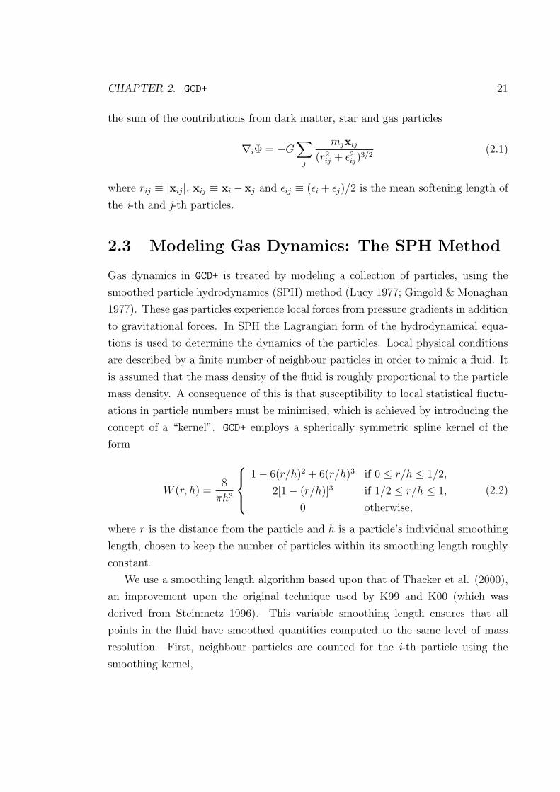
Figure 2.1: Cooling rates, plotted as a function of temperature, for the metallicities indi-cated. Linear interpolation of these curves is used to calculate cooling rates as a function oftemperature and metallicity.
2.4 Radiative Gas Cooling
The temperature of gas particles in GCD+ is derived by Ti = Piµmp/(kBρi), where
Pi and ρi are the pressure and density of the i-th particle, µ is the mean molecular
weight, kB is Boltzmann’s constant and mp is the proton mass. For simplicity, the
mean molecular weight is set to µ=0.6, independent of metallicity. The lower limit
to the calculated temperature is Tlim=100 K, unless otherwise stated. Radiative
cooling of gas is modeled using the cooling curves of MAPPINGS III (Sutherland &
Dopita, 1993). It is important to use metallicity-dependent models due to the strong
role played by metals in radiatively cooling gas (Kaellander & Hultman 1998; Kay
et al. 2000) . The models adopted in GCD+ are shown in figure 2.1. It is assumed
that gas with metallicity below [Fe/H]= −3 cools at the same rate as gas with
[Fe/H]= −3, and that the cooling rate for gas with [Fe/H]> 0.5 is the same as that
for [Fe/H]= 0.5. The cooling rates for −3 <[Fe/H]< 0.5 are calculated, as a function
of the temperature and metallicity of each gas particle, by linear interpolation of
the cooling curves.
CHAPTER 2. GCD+ 27
2.5 Star Formation
Star formation prescriptions similar to those of Katz (1992) and Katz, Weinberg &
Hernquist (1996) were employed. Star formation occurs whenever
1. the gas density is greater than a critical density:
ρcrit = 2× 10⁻²⁵ g cm−3 (Katz et al. 1996),
2. the gas velocity field is convergent: ∇ · vi < 0, and
3. the gas is Jeans unstable, i.e. h/vs > τg, where h is the smoothing length, vs
the speed of sound, and τg =√
3π/16Gρg is the dynamical time of the gas.
The adopted star formation law is written
dρ∗dt
= −dρgdt
=c∗ρgτg
(2.27)
where dρ∗dt
is the star formation rate (SFR). Equation (2.27) corresponds to a Schmidt
law in which the SFR is proportional to ρ1.5g . The star formation timescale is assumed
to be the local dynamical timescale, τg =√
(3π/16Gρg) because in regions eligible
for star formation, the dynamical timescale is generally longer than the cooling
timescale. Star formation efficiency is parameterised by the dimensionless parameter
c∗.
Equation (2.27) implies that the probability, p∗, with which one gas particle
entirely transforms into a star particle during a discrete time step, ∆t, is p∗ =
1 − exp(−c∗∆t/tg). Entirely transforming gas particles into star particles, using
such a probabilistic approach, avoids the creation of an intolerably large number
of star particles of different masses being formed. The newly created star particle
behaves as a collisionless particle, as described in section 2.2.
2.6 Initial Mass Function
In GCD+ simulations, “stars” are represented as particles, which for the simulations
described here have a typical mass of 105−106 M. The relative number distribution
of stellar masses within a star particle at its birth is governed by the assumed
initial mass function (IMF). Variation of this IMF, in particular with respect to low
metallicity stars, is central to our feasibility study concerning white dwarfs being a
CHAPTER 2. GCD+ 28
significant component of the dark matter of the halo of Milky Way (chapter 3). In
other studies presented in this thesis, the IMF is considered to be universal, with the
canonical Salpeter (1955) form adopted. The Salpter IMF is written (by number)
Φ(m)dm = dn/dm = Am−(1+x) dm, (2.28)
with x=1.35. The coefficient A in equation (3.3) is determined by normalising the
IMF to unity over the specified range of stellar masses.
2.7 Feedback
GCD+ takes into account metal enrichment and energy released by both Type II
(SNe II) and Type Ia (SNe Ia) supernovae, as well as the metal enrichment from
intermediate mass stars. The event rates and yields of SNe II and SNe Ia, and the
yields of intermediate mass stars, are calculated for each particle at each time-step,
by taking into account the IMF and stellar lifetimes.
The amount of mass, energy, and heavy elements released by SNe is smoothed
over neighbouring gas particles using the SPH kernel (Katz 1992). For example, in
the time-step in which mass Mej,i is ejected from the i-th star particle, the increment
of the mass of the j-th neighbour particle is
∆Mej,j =mj
ρg,iMej,iW (rij, hij) (2.29)
where
ρg,i = 〈ρg(xi)〉 =∑
j 6=imjW (rij, hij) (2.30)
and W (rij, hij) is the SPH kernel (equation 2.2).
2.7.1 Supernovae
It is assumed that each massive star (≥8 M) explodes as a SNe II. Rates for SNe Ia
are calculated following the model proposed by Kobayashi, Tsujimoto & Nomoto
(2000, KTN00 hereafter). This model assumes that SNe Ia occur in binary systems
which consist of primary and companion stars with appropriate masses. The model
also assumes that SNe Ia do not occur in low metallicity stars with [Fe/H]< −1.1
CHAPTER 2. GCD+ 29
(although this is implemented in GCD+ by using total metallicity rather than iron
abundance, logZ/Z < −1.1).
In this formalism, primary stars have main-sequence masses in the range of
mp,l = 3 M and mp,u = 8 M, and evolve into C+O white dwarfs (WDs). The
mass range of companion stars are restricted to being between md,RG,l = 0.9 M and
md,RG,u = 1.5 M for low-mass red giants, with the system designated a ’RG+WD
system’ and between md,MS,l = 1.8 M md,MS,u = 2.6 M for slightly evolved main
sequence companions, designated a ’MS+WD system’. The total number of SNe Ia
is then obtained as a function of age, t, of a star particle with the mass of ms M,
via
NSNeIa(t) = ms
∫ mp,u
mp,l
m−(1+x)dm
∫ Mu
Ml
m−xdm
−1
×[bMS
∫ md,MS,u
max(md,MS,l ,mt)Φd(m)dm
∫ md,MS,u
md,MS,lΦd(m)dm
+ bRG
∫ md,RG,umax(md,RG,l ,mt)
Φd(m)dm∫ md,RG,umd,RG,l
Φd(m)dm
], (2.31)
where mt is the mass of a star whose lifetime is equal to t, and the mass function of
the companion stars is assumed to be Φd(m) ∝ m−0.35, following KTN00. The term
before the square bracket indicates the number of C+O WDs, i.e. primary stars.
The first term within the square bracket determines the fraction of C+O WDs which
evolve into SNe Ia from MS+WD systems, and the second term determines the
fraction of C+O WDs which evolve into SNe Ia from RG+WD systems. Following
KTN00, we set bMS = 0.05 and bRG = 0.02. The nucleosynthesis prescriptions for
SNe Ia are taken from the W7 model of Iwamoto et al. (1999).
2.7.2 Heavy Elements
The evolution of several chemical elements are followed in GCD+; 1H, 4He, 12C, 14N,16O, 20Ne, 24Mg, 28Si, 56Fe and total metallicity, Z. The stellar yields of Woosley
& Weaver (1995, hereafter WW95) are used to provide the mass of gas and metals
ejected by SNe II. These provide yields for stars between the mass range 11 M
and 40 M (using their ’B’ Model for stars greater than 30 M). For masses above

CHAPTER 2. GCD+ 30
Figure 2.2: Chemical yields of a burst of star formation of mass 1 M as a function of time.The upper (lower) panel shows the total ejected oxygen (iron) mass. The history of a starparticle are shown for two metallicities, Z=0.02 (thick line) and Z=10−4 (thin line).
CHAPTER 2. GCD+ 31
40 M the same abundance ratios for stars of mass 40 M are assumed. The yields of
WW95 are metallicity dependent, and the code makes linear interpolations between
grids of different metallicity to calculate the yields.
For intermediate mass stars (≤8 M) yields and remnant masses are taken from
van den Hoek & Groenwegen (1997), which provide metallicity dependent yields of1H, 4He, 12C, 14N and 16O for stars in the mass range 0.8 M-8 M. Abundances
for 20Ne, 24Mg, 28Si, and 56Fe are scaled to the solar abundance set. Yields for
stars in the mass range 8 M-11 M remain uncertain, so linear interpolation is used
between yields of the most massive stars in the van den Hoek & Groenwegen (1997)
tables and the lowest mass stars in the tables of WW95.
A further uncertainty is in the yields from zero metallicity stars. We simply use
the yields from the lowest metallicity stars in the vdHG tables, i.e. Z= 0.001, for
all stars with lower metallicity. Recent yields of Limongi & Chieffi (2003) indicate
that this simplification will not have a dramatic effect. It is important though
to acknowledge those particular studies for which such an assumption could be
problematic. This is the case for our study of a putative white dwarf dominated
Galactic halo (chapter 3).
A look-up table of all yields, remnant masses and number of SNe as a function
of a star particle’s age and metallicity is used for each star particle at each time-
step. Here, we use the stellar lifetimes adopted by Kodama (1997) and Kodama &
Arimoto (1997). Figure 2.2 shows the total amount of oxygen and iron ejected from
a 1 M burst of star formation as a function of time. Metals are initially ejected
by SNe II, which produce most of the oxygen. After SNe II cease, at the time of
death of an 8 M star, any additional oxygen ejection is due to intermediate-mass
stars. The timescale for iron production is set by the lifetime of the secondary in
the binary systems which lead to SNe Ia.
2.7.3 Energy Feedback
Structure formation in our models is driven by dark matter, initially expanding with
the Hubble flow, then collapsing due to local overdensities. Gas initially traces this
dark matter, with star formation triggered within the most dense regions. When
the most massive of these stars end their lives they “feedback” energy into the
surrounding ISM, affecting galaxy evolution on a global scale. These effects are seen
on scales ranging from the inter galactic medium and galaxy clusters, to globular

CHAPTER 2. GCD+ 32
cluster and dwarf galaxies.
The implementation of energy feedback into galaxy formation codes remains a
challenge. In a simulation by Katz (1992), energy feedback was implemented by
depositing thermal energy into the surrounding gas, using the SPH kernel. This
form of energy feedback was found to be inefficient, as the regions in which star
formation is occurring are, by design, high density regions, and hence have short
cooling timescales. Thus the thermal energy is radiated away rapidly, without regu-
lating star formation. The model assumes that SNe energy affects the temperature
of the surrounding gas, thereby increasing the internal energy of neighbour particles.
Hence, when the i-th particle ejects SNe energy of ESN,i, it deposits energy ∆ESN,j
in the j-th neighbour gas particle, using the smoothing kernel
∆ESN,j = ESN,imj
ρg,iW (ri,j, hi,j). (2.32)
In GCD+ it is assumed that each SNe yields an energy of εSN × 1051 ergs.
The difficulties in implementing feedback in galaxy evolution codes and the prob-
lems that result in terms of simulating galaxy formation are examined in some detail
in our study of disk galaxy formation in chapter 5. It is important in our studies
to be aware of these problems and to be aware of their potential effects on the
particular aspect of galaxy formation which is being probed.

Chapter 3
Simulating a White Dwarf
dominated Halo
3.1 Introduction
Evidence gathered by microlensing surveys toward the Large Magellanic Cloud sug-
gest that a substantial fraction of the Milky Way’s dark matter halo is comprised
of ∼0.5 M objects: the MACHO Team claim 20% of the halo’s dynamical mass
may be tied up in these half-solar mass constituents (Alcock et al. 2000), while
the EROS Team favour an upper limit of 30% (Lasserre et al. 2000). Constraints
set by Hubble Space Telescope red star counts (Flynn et al. 1996) rule out large
numbers of low-mass hydrogen burning stars in the halo. By process of elimina-
tion, white dwarfs represent one potential baryonic candidate for these microlensing
events. This would correspond to of order 2×10¹¹ white dwarfs out to a distance of
60 kpc in the Galactic halo (see Zritsky 1999).
The apparent identification of 2-5 high proper motion white dwarfs in the Hubble
Deep Field-North supported the white dwarf-dominated halo hypothesis (Ibata et al.
1999), as did the colour analysis of the Hubble Deep Field-South (Mendez et al.
2000). The Ibata et al. claim has since been retracted (Richer 2001). Ground-based
searches for nearby high-proper motion white dwarfs initially suggested a white
dwarf halo mass fraction of 10% (Ibata et al. 2000), although Flynn et al. (2001)
favoured <∼ 2%. Based upon dynamical arguments and Galactic winds driven by a
putative population of white dwarf progenitors, Zhao (2002) suggest a fraction <4%.
Regardless, Oppenheimer et al. (2001, hereafter OHDHS) have recently revived the
33

CHAPTER 3. SIMULATING A WHITE DWARF DOMINATED HALO 34
white dwarf-dominated halo picture with their claim that >2% of the halo is made
up of white dwarfs. While criticism of the OHDHS analysis is appreciable (Gibson
& Flynn 2001; Reid et al. 2001; Reyle et al. 2001; Flynn et al. 2003; Torres et al.
2002), their result (if confirmed) may yet be made consistent with the MACHO and
EROS Team results1
White dwarfs represent the end point in the life cycle of stars with initial masses
in the approximate range 1 − 8 M. Populating a white dwarf-dominated Galactic
halo, in conjunction with a standard stellar initial mass function (IMF), would lead
to a corresponding increase in the production of Type II supernovae (SNeII) and the
rapid overproduction of heavy elements (Gibson & Mould 1997, hereafter GM97).
In addition, the expected number of low-mass red dwarfs would violate the deep halo
star counts of Flynn et. al. (1996). These high- and low-mass constraints imply that
a standard IMF cannot be employed to populate a putative white dwarf-dominated
Galactic halo. Instead, the IMF would have had to have been comprised almost
exclusively of stars in the range 1 <∼ m/M <∼ 8; such white dwarf-heavy IMFs have
been discussed in the literature by Chabrier et al. (1996, hereafter C96) and Adams
& Laughlin (1996).
Besides the requirement that any white dwarf-heavy IMF be restricted to
1 <∼ m/M <∼ 8, there is an additional constraint provided by the observed abun-
dance patterns in Population II halo stars. GM97 found that a white dwarf-
dominated IMF (wdIMF) inevitably leads to the overproduction of carbon and
nitrogen relative to oxygen - by more than an order of magnitude - in compari-
son with that seen in the oldest stars of the Milky Way’s halo. This result is a
natural consequence of the life cycle of low- and intermediate-mass stars, the stars
which are responsible for synthesising the majority of the carbon and nitrogen in
the Universe. Fields et al. (2000) confirmed the analysis of GM97, concluding that
the carbon and nitrogen content of the halo provides the strictest constraint to any
white dwarf-dominated halo scenario.
While there is no compelling direct evidence for variable IMFs, at the present
time (e.g. Gilmore 2001), several theoretical studies suggest that the IMF of the first
1Note that Nelson et al. (2002) claim a 7% white dwarf dark halo based upon 24 candidatehigh-proper motion objects in the Groth Strip. Likewise Mendez (2002) argues that most of thedark matter in the solar vincinity can be accounted for by halo and thick-disk white dwarfs (albeitbased upon one apparent high-proper motion white dwarf seen towards NGC 6397). The EROS-2white dwarf proper motion survey find that the halo white dwarf fraction cannot exceed 5% (95%c.l.).
CHAPTER 3. SIMULATING A WHITE DWARF DOMINATED HALO 35
generation of stars (so-called Population III) might be quite different from that of the
canonical Salpeter IMF (sIMF). Direct attempts to form Pop III stars in numerical
simulations indicate an IMF biased toward super massive stars (M > 100 M) rather
than white dwarf progenitors (Abel, Bryan & Norman 1999, 2002). It is the lack of
metals, which cause cloud fragmentation of gas in star forming regions, that results
in such a top heavy IMF (see also Bromm et. al 2001). Other studies also indicate a
different IMF for Pop III stars, e.g. Yoshii & Saio (1987) and Nakamura & Umemura
(2001), the latter study proposing a bimodal IMF that produces large numbers of
super massive stars around 100 M and a futher peak in the intermediate, white
dwarf progenitor mass range. It is possible that the stars from the high mass peak
of such an IMF would not contribute to chemical enrichment due to the formation
of black holes, thus making such an IMF effectively favour white dwarf progenitors.
This Pop III IMF is expected to apply to the first generation of halo stars - the
generation which would manifest itself now in the population of putative high-proper
motion stellar halo white dwarfs. Such studies remain, however, highly uncertain.
Our motivation for invoking the wdIMF remains the MACHO observations and the
necessity for invoking such an IMF in order for these observations to be explained
by a large population of white dwarf stars populating the halo. In addition to the
wdIMF and sIMF possibilities, in what follows we will also consider a variable IMF in
which stars formed from the low (high) metallicity gas are distributed following the
adoption of the wdIMF (sIMF). One can anticipate that while the wdIMF phase will
invariably lead to high C/O and N/O ratios (as discussed by GM97), the subsequent
sIMF phase can ameliorate this effect. A variable IMF scenario was not considered
by GM97.
The currently favoured hierarchical clustering scenario of galaxy formation pos-
tulates that star formation progresses through the on-going accretion of galactic
building blocks. Within this framework, highly inhomogeneous chemical evolution
occurs; homogeneous closed-box models for the Milky Way’s evolution (as were
adopted by GM97) are no longer suitable. The early phases of galaxy formation
demand a chemo-dynamical approach, one which we adopt here explicitly within
the context of the white dwarf-dominated IMF hypothesis. In what follows, we
examine the ability of metallicity-dependent variable IMFs to resolve the apparent
contradiction between a significantly white dwarf-heavy Galactic halo and the C/O
and N/O abundance patterns of halo stars. To achieve this, we perform numerical
simulations that calculate the chemical and dynamical evolution of a Milky Way-like

CHAPTER 3. SIMULATING A WHITE DWARF DOMINATED HALO 36
galaxy in a self-consistent manner.
In section 3.2, we describe our numerical methods, concentrating upon the code
itself and our treatments of star formation, IMFs, and energy feedback to the inter-
stellar medium (ISM). Section 3.3 presents the results of our simulations in terms
of resulting white dwarf halo densities, and Galactic chemical evolution of carbon,
nitrogen, and oxygen. The implications for a white dwarf-dominated Galactic dark
matter halo are described in section 3.4.
3.2 Method
3.2.1 The Code
Our simulations were performed using a modified version of the software package
described by Kawata (1999, 2001). An overview of the code is provided here along
with the relevant modifications made for the current study - the reader is referred
to Kawata (1999, 2001) for all other details. Our code is based upon the Hern-
quist & Katz 1989 and Katz, Weinberg & Hernquist 1996 TreeSPH, combining a
tree algorithm (Barnes & Hut 1986) with smoothed particle hydrodynamics (SPH)
(Lucy 1977; Gingold & Monaghan 1977) for the computation of gravitational forces
and numerical hydrodynamics respectively. This three-dimensional code is fully La-
grangian, with individual smoothing lengths and time-steps making it highly adap-
tive in space and time. It includes a self-consistent treatment of physical processes
governing galaxy formation, including self-gravity, hydrodynamics, radiative cooling,
star formation, supernovae feedback, and metal enrichment. We employ metallicity-
dependent gas cooling rates derived from MAPPINGS III (Sutherland & Dopita
1993); their implementation is described by Kawata & Gibson (2003a).
Star Formation
Star formation prescriptions similar to those of Katz (1992) and Katz, Weinberg &
Hernquist (1996) were employed. Star formation occurs whenever
1. the gas density is greater than a critical density:
ρcrit = 2× 10⁻²⁵ g cm−3 (Katz et al. 1996), and
2. the gas velocity field is convergent: ∇ · vi < 0.

CHAPTER 3. SIMULATING A WHITE DWARF DOMINATED HALO 37
Our adopted star formation law is written
dρ∗dt
= −dρgdt
=c∗ρgτg
(3.1)
where dρ∗dt
is the star formation rate (SFR). Equation 3.1 corresponds to a Schmidt
law in which the SFR is proportional to ρ1.5g . The dynamical timescale of the gas is
given by τg =√
(3π/16Gρg); in regions eligible for star formation, this dynamical
timescale is generally longer than the cooling timescale. Star formation efficiency is
parameterised by the dimensionless parameter c∗, which, after Kawata (1999, 2001),
is set to c∗ = 0.5.
Equation 3.1 implies that the probability, p∗, with which one gas particle en-
tirely transforms into a star particle during a discrete time step, ∆t, is p∗ =
1 − exp(−c∗∆t/tg). This avoids an intolerably large number of star particles of
different masses being formed. The newly created star particle behaves as a colli-
sionless particle.
Initial Mass Functions
In our TreeSPH simulations, stars are represented as particles with a typical mass of
order 105 M; the relative number distribution of stellar masses within a “particle” is
governed by the assumed initial mass function (IMF). Fundamental to our modeling
is the adoption of the Chabrier et al. (1996) white dwarf progenitor-dominated IMF
(wdIMF). We represent this IMF by a truncated power-law of the form
Φ(m) dm = dn/dm = Ae−(m/m)β ×m−α dm (3.2)
for which we use m = 2.7, β = 2.2, and α = 5.75. The peak of this wdIMF occurs
at m ≈ 2 M, favouring the production of white dwarf progenitors.
The canonical Salpeter (1955) IMF (sIMF) is used to describe the local stellar
mass function (by number) and is written
Φ(m)dm = dn/dm = Am−(1+x) dm, (3.3)
with x=1.35. The sIMF (red line) and wdIMF (green line) are shown in figure 3.1.
The coefficient A in equations 3.2 and 3.3 is determined by normalising the
respective IMFs over the mass range 0.1≤m/M≤40.0. We explore simulations in
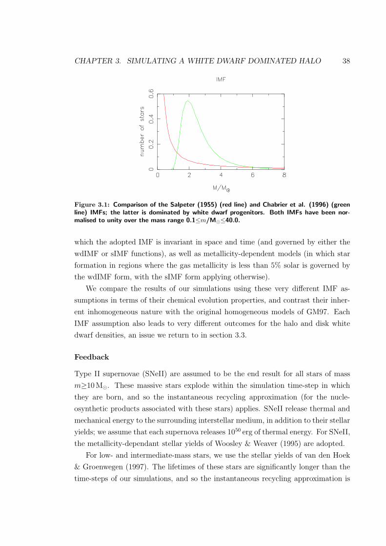
CHAPTER 3. SIMULATING A WHITE DWARF DOMINATED HALO 38
Figure 3.1: Comparison of the Salpeter (1955) (red line) and Chabrier et al. (1996) (greenline) IMFs; the latter is dominated by white dwarf progenitors. Both IMFs have been nor-malised to unity over the mass range 0.1≤m/M≤40.0.
which the adopted IMF is invariant in space and time (and governed by either the
wdIMF or sIMF functions), as well as metallicity-dependent models (in which star
formation in regions where the gas metallicity is less than 5% solar is governed by
the wdIMF form, with the sIMF form applying otherwise).
We compare the results of our simulations using these very different IMF as-
sumptions in terms of their chemical evolution properties, and contrast their inher-
ent inhomogeneous nature with the original homogeneous models of GM97. Each
IMF assumption also leads to very different outcomes for the halo and disk white
dwarf densities, an issue we return to in section 3.3.
Feedback
Type II supernovae (SNeII) are assumed to be the end result for all stars of mass
m≥10 M. These massive stars explode within the simulation time-step in which
they are born, and so the instantaneous recycling approximation (for the nucle-
osynthetic products associated with these stars) applies. SNeII release thermal and
mechanical energy to the surrounding interstellar medium, in addition to their stellar
yields; we assume that each supernova releases 1050 erg of thermal energy. For SNeII,
the metallicity-dependant stellar yields of Woosley & Weaver (1995) are adopted.
For low- and intermediate-mass stars, we use the stellar yields of van den Hoek
& Groenwegen (1997). The lifetimes of these stars are significantly longer than the
time-steps of our simulations, and so the instantaneous recycling approximation is
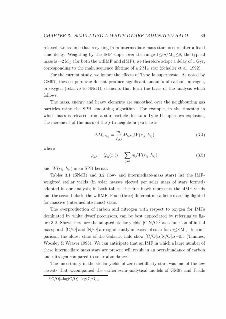
CHAPTER 3. SIMULATING A WHITE DWARF DOMINATED HALO 39
relaxed; we assume that recycling from intermediate mass stars occurs after a fixed
time delay. Weighting by the IMF slope, over the range 1≤m/M≤8, the typical
mass is ∼2 M (for both the wdIMF and sIMF); we therefore adopt a delay of 1 Gyr,
corresponding to the main sequence lifetime of a 2 M star (Schaller et al. 1992).
For the current study, we ignore the effects of Type Ia supernovae. As noted by
GM97, these supernovae do not produce significant amounts of carbon, nitrogen,
or oxygen (relative to SNeII), elements that form the basis of the analysis which
follows.
The mass, energy and heavy elements are smoothed over the neighbouring gas
particles using the SPH smoothing algorithm. For example, in the timestep in
which mass is released from a star particle due to a Type II supernova explosion,
the increment of the mass of the j-th neighbour particle is
∆MSN,j =mj
ρg,iMSN,iW (rij, hij) (3.4)
where
ρg,i = 〈ρg(xi)〉 =∑
j 6=imjW (rij, hij) (3.5)
and W (rij, hij) is an SPH kernal.
Tables 3.1 (SNeII) and 3.2 (low- and intermediate-mass stars) list the IMF-
weighted stellar yields (in solar masses ejected per solar mass of stars formed)
adopted in our analysis; in both tables, the first block represents the sIMF yields
and the second block, the wdIMF. Four (three) different metallicities are highlighted
for massive (intermediate mass) stars.
The overproduction of carbon and nitrogen with respect to oxygen for IMFs
dominated by white dwarf precursors, can be best appreciated by referring to fig-
ure 3.2. Shown here are the adopted stellar yields’ [C,N/O]2 as a function of initial
mass; both [C/O] and [N/O] are significantly in excess of solar for m≤8 M. In com-
parison, the oldest stars of the Galactic halo show [C/O]'[N/O]'−0.5 (Timmes,
Woosley & Weaver 1995). We can anticipate that an IMF in which a large number of
these intermediate mass stars are present will result in an overabundance of carbon
and nitrogen compared to solar abundances.
The uncertainty in the stellar yields of zero metallicity stars was one of the few
caveats that accompanied the earlier semi-analytical models of GM97 and Fields
2[C/O]≡log(C/O)−log(C/O)

CHAPTER 3. SIMULATING A WHITE DWARF DOMINATED HALO 40
Table 3.1: IMF-weighted stellar yields adopted for massive (m≥10 M) stars.
Salpeter (1955) - sIMFMetallicity 0.0 ≤ Z/Z < 10−4 10−4 ≤ Z/Z < 10−1 10−1 ≤ Z/Z < 1.0 1.0 ≤ Z/Z
ElementC 6.12× 10⁻⁴ 8.46× 10⁻⁴ 8.39× 10⁻⁴ 8.53× 10⁻⁴
O 2.74× 10⁻³ 5.99× 10⁻³ 6.55× 10⁻³ 7.26× 10⁻³
N 3.25× 10⁻⁵ 3.20× 10⁻⁵ 6.09× 10⁻⁵ 3.05× 10⁻⁴
Ne 2.08× 10⁻⁴ 7.32× 10⁻⁴ 5.47× 10⁻⁴ 6.92× 10⁻⁴
Mg 1.42× 10⁻⁴ 2.83× 10⁻⁴ 3.17× 10⁻⁴ 4.14× 10⁻⁴
Si 1.80× 10⁻⁴ 5.88× 10⁻⁴ 6.06× 10⁻⁴ 7.60× 10⁻⁴
Fe 4.78× 10⁻⁴ 4.76× 10⁻⁴ 7.86× 10⁻⁴ 7.05× 10⁻⁴
[C/O] −0.16 −0.35 −0.40 −0.44[N/O] −0.98 −1.33 −1.09 −0.44
Chabrier et al. (1996) - wdIMFC 3.62× 10⁻⁶ 5.49× 10⁻⁶ 6.06× 10⁻⁶ 5.77× 10⁻⁶
O 7.71× 10⁻⁶ 1.47× 10⁻⁵ 1.76× 10⁻⁵ 2.12× 10⁻⁵
N 1.20× 10⁻⁶ 1.21× 10⁻⁶ 1.47× 10⁻⁶ 3.31× 10⁻⁶
Ne 8.66× 10⁻⁷ 6.14× 10⁻⁶ 1.61× 10⁻⁶ 3.07× 10⁻⁵
Mg 5.63× 10⁻⁷ 7.32× 10⁻⁷ 8.30× 10⁻⁷ 1.36× 10⁻⁶
Si 1.72× 10⁻⁶ 3.62× 10⁻⁶ 2.92× 10⁻⁶ 4.04× 10⁻⁶
Fe 6.00× 10⁻⁶ 3.94× 10⁻⁶ 1.02× 10⁻⁵ 6.41× 10⁻⁶
[C/O] 0.167 0.067 0.032 −0.070[N/O] 0.14 −0.14 −0.13 0.13

CHAPTER 3. SIMULATING A WHITE DWARF DOMINATED HALO 41
Table 3.2: IMF-weighted stellar yields adopted for low- and intermediate-mass (m≤8 M)stars.
Salpeter (1955) - sIMFMetallicity 5× 10⁻³ ≤ Z/Z < 10−1 10−1 ≤ Z/Z < 1.0 1.0 ≤ Z/Z
ElementC 6.82× 10⁻⁴ 7.26× 10⁻⁴ 1.20× 10⁻³
O 1.27× 10⁻⁵ 1.18× 10⁻⁴ 1.11× 10⁻³
N 1.32× 10⁻³ 1.37× 10⁻³ 1.21× 10⁻³
Ne 1.06× 10⁻⁵ 1.56× 10⁻⁵ 2.36× 10⁻⁵
Mg 5.95× 10⁻⁷ 1.19× 10⁻⁵ 1.26× 10⁻⁴
Si 6.46× 10⁻⁷ 1.29× 10⁻⁵ 1.36× 10⁻⁴
Fe 1.07× 10⁻⁶ 2.14× 10⁻⁵ 2.26× 10⁻⁴
[C/O] 2.22 1.28 0.529[N/O] 2.95 2.00 0.97
Chabrier et al. (1996) - wdIMFC 3.96× 10⁻³ 3.10× 10⁻³ 3.96× 10⁻³
O 7.67× 10⁻⁵ 4.54× 10⁻⁴ 4.31× 10⁻³
N 2.42× 10⁻³ 1.43× 10⁻³ 1.74× 10⁻³
Ne 3.32× 10⁻⁵ 5.70× 10⁻⁵ 8.60× 10⁻⁵
Mg 9.81× 10⁻⁷ 4.47× 10⁻⁵ 4.70× 10⁻⁴
Si 1.07× 10⁻⁶ 4.85× 10⁻⁵ 5.11× 10⁻⁴
Fe 1.76× 10⁻⁶ 8.05× 10⁻⁵ 8.48× 10⁻⁴
[C/O] 2.21 1.32 0.46[N/O] 2.44 1.43 0.54
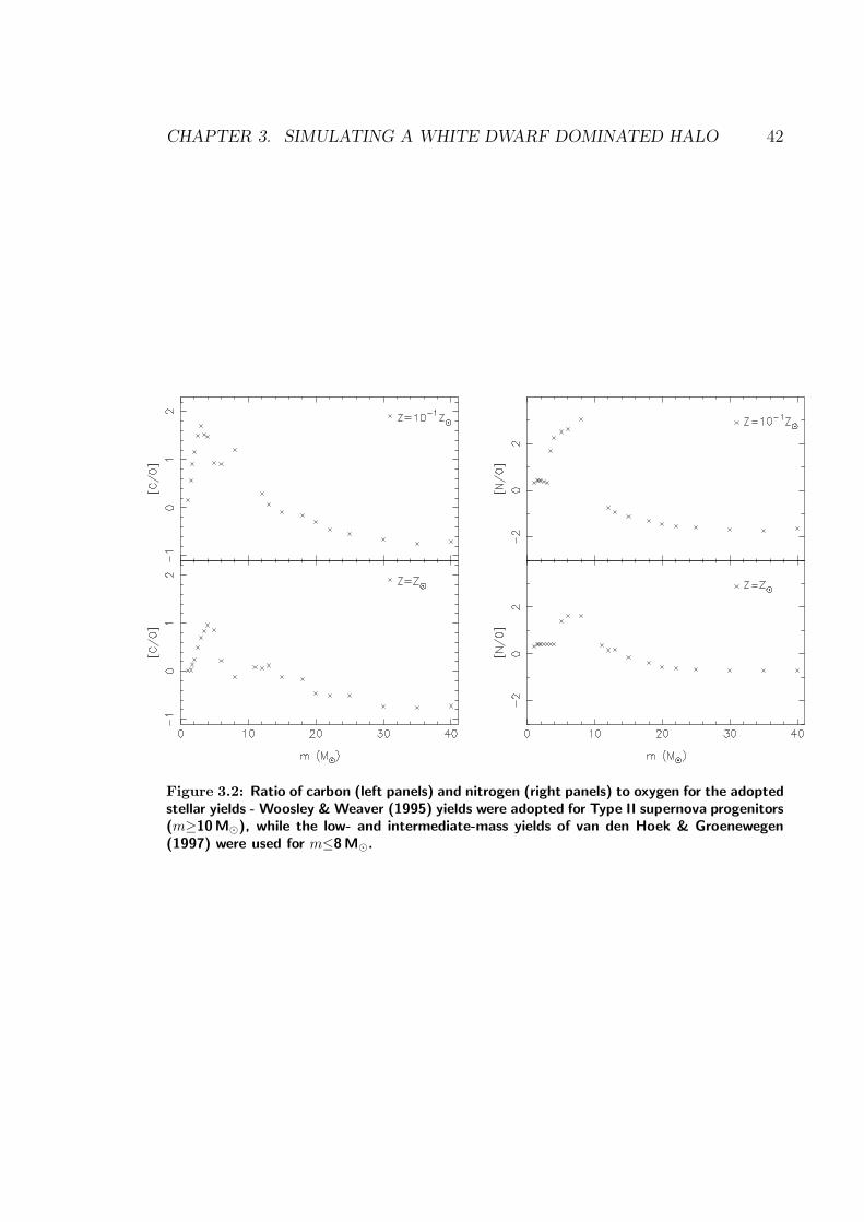
CHAPTER 3. SIMULATING A WHITE DWARF DOMINATED HALO 42
Figure 3.2: Ratio of carbon (left panels) and nitrogen (right panels) to oxygen for the adoptedstellar yields - Woosley & Weaver (1995) yields were adopted for Type II supernova progenitors(m≥10 M), while the low- and intermediate-mass yields of van den Hoek & Groenewegen(1997) were used for m≤8 M.

CHAPTER 3. SIMULATING A WHITE DWARF DOMINATED HALO 43
et al. (2000). As noted by Marigo et al. (2001) “the distinct evolutionary behaviour
of these (zero metallicity) stars may also imply a very distinct nucleosynthesis and
chemical pollution of the interstellar medium”; at issue here is the production of car-
bon and nitrogen in Population III stars. If it could be shown that neither element
was synthesised or ejected into the ISM in the early Universe, a “loophole” could
then exist that would allow a white dwarf-dominated Galactic halo without violat-
ing the elemental abundance patterns in the halo today. The new stellar evolution
models described by Abia et al. (2001) suggest that large quantitative differences
do not exist between extant low-metallicity models (which undergo thermal pulses
and eject significant carbon and nitrogen) and Population III (at least for masses
4≤m/M≤7; for masses m≤4 M, the Population III yields remain uncertain). Our
models are qualitatively robust against the specific choice of yield compilation.
3.2.2 The Model
We calculate semi-cosmological models, following the technique described by Kawata
(1999, 2001). Our seed galaxy is an isolated sphere upon which small-scale den-
sity fluctuations corresponding to a cold dark matter (CDM) power spectrum are
superimposed. These initial density fluctuations are generated using COSMICS
(Bertschinger 1995). The effects of longer wavelength fluctuations are incorporated
by enhanced density of the sphere and the application of a spin parameter λ re-
sponsible for initiating rigid rotation of the overdense sphere. This spin parameter
is defined
λ ≡ J |E|1/2GM
5/2tot
, (3.6)
where E is the total energy of the system, J the total angular momentum, Mtot the
total mass of the sphere (dark matter + gas). Mass fluctuations (rms) in a sphere of
radius 8h−1 Mpc are denoted σ8,in, and normalise the amplitude of the CDM power
spectrum. According to Katz & Gunn (1992) and Steinmetz & Muller (1995), a large
value of σ8,in leads a large transfer of angular momentum from the gas particles to
the dark matter particles, and a bulge larger than observed in the Milky Way; in
order to avoid this, we consider the Galaxy to be formed in an environment where
the small scale density perturbation is smoother than the mean value suggested in
standard CDM cosmology. We set σ8,in = 0.1. The expected collapse redshift is
given by zc. The amplitude of the top-hat density perturbation δi is approximately

CHAPTER 3. SIMULATING A WHITE DWARF DOMINATED HALO 44
Table 3.3: The three models adopted in the current analysis; the initial mass function (IMF)is the only variable.
IMFModel Z < 0.05 Z Z > 0.05 Z
model 1 Salpeter Salpetermodel 2 Chabrier Chabriermodel 3 Chabrier Salpeter
related to initial and collapse redshift by zc = 0.36δi(1 + zi) − 1 (Padmanabham
1993). Thus δi is determined for a given zc at zi. We set zc = 2.0. The simulated
galaxies described here have total mass Mtot = 5×10¹¹ M, approximating the total
mass of the Milky Way within 50 kpc (Wilkinson & Evans 1999). For our models,
the initial conditions are uniquely determined by the choice of λ, Mtot, σ8,in, and zc.
Using a comparable semi-cosmological model, Katz & Gunn (1991) found that
a seed galaxy with a large spin parameter evolves into a disk system. Our best
Milky Way models require λ = 0.07, in order to remain consistent with the Galaxy’s
present-day disk properties. We assume a flat (Ωo = 1) universe with baryon fraction
Ωb = 0.1 and Hubble constant Ho = 50 kms−1 Mpc−1; evolution within isolated
galaxy simulations using top hat overdensities are not greatly influenced by choice
of cosmology. Evolution is traced from an initial redshift zi = 40 to the present.
The initial conditions used are somewhat artificial, and do not exactly reflect
hierarchical formation of the Milky Way as expected in CDM cosmologies. However,
this approach still traces hierarchical build up of a galaxy, self-consistently treating
its chemical and dynamical history, and is sufficient for the purposes of documenting
the effects between different IMFs.
Our study relies on the chemical enrichment processes of SPH, as described in
section 3.2.1. In order to ensure that such processes are not determined by the
resolution adopted, we perform the study at three different resolution regimes. The
resolution regimes employ 6142, 18342, and 40958 particles (initially split evenly be-
tween gas and dark matter). The results presented in this paper are from the highest
resolution models; the results of different resolution regimes varied only marginally
quantitatively, and the analysis and conclusions presented hold in all three; we
therefore only present the highest resolution models. Our highest resolution models
have dark matter (baryonic) particles of mass 2.2 × 10⁶ M (2.4 × 10⁵ M), which
CHAPTER 3. SIMULATING A WHITE DWARF DOMINATED HALO 45
Figure 3.3: Density plot of the projection onto the X-Y plane of the evolution of stars (upperrow) and gas (bottom row) during the major star forming epoch of model 3.
is comparable in resolution with other recent simulations of disk galaxy formation
(e.g. Abadi et. al 2003)3. The gravitational softening length is 0.79 kpc (1.6 kpc)
for baryonic (dark matter) particles.
As noted earlier, the primary “variable” in our simulations is the initial mass
function (IMF). Three different scenarios have been considered here - models 1 and 2
assume the Salpeter (1955) and Chabrier et al. (1996) IMFs, respectively, regardless
of metallicity; model 3 assumes the Chabrier et al. IMF (wdIM) for metallicities
below 5% solar, and the Salpeter IMF (sIMF) elsewhere, as summarised in table 3.3.
3.3 Results
Figures 3.3 and 3.4 show the X-Y and X-Z projections of the morphological
evolution for model 3, over the redshift range z = 2.7 to z = 0.9; models 1 and 2
are qualitatively similar. The Z-axis corresponds to the initial rotation axis. Sub-
clumps associated with early star formation can be traced to initial small-scale
density fluctuations, and are clearly seen by redshift z ≈ 2.5. These sub-clumps
3In galaxy formation simulations including cooling, the physical resolution determines the com-putational costs rather than the total number of particles.

CHAPTER 3. SIMULATING A WHITE DWARF DOMINATED HALO 46
Figure 3.4: Density plot of the projection onto the X-Z plane of the evolution of stars (upperrow) and gas (bottom row) during the major star forming epoch of model 3.
merge hierarchically until redshift z ≈ 1.7; by redshift z ≈ 1.6, large sub-clumps
merging in the centre of the Galaxy (where the disk is forming) is responsible for
the bulk of star formation. An epoch of accretion (1.2 <∼ z <∼ 0.9) witnesses the
formation of the majority of the high-metallicity (Z > 0.05Z) stars, and the disk-
like structure of the Galaxy becomes evident. The star formation histories of the
three models are shown in figure 3.5. The system barely evolves morphologically
after redshift z ≈ 0.8. While not shown, we confirm that the radial scale lengths for
our simulated disk at z = 0 (both gas and stellar) match those of the Milky Way.
Density maps of the final distributions (z = 0) of star and gas particles for
model 3 are shown in figure 3.6. The X-Y (upper row) and X-Z (bottom row)
planes are shown. Note that the low-metallicity (Z < 0.05Z) stars of the Galaxy
preferentially populate the halo and thick disk, while the metal-rich (Z > 0.05Z)
component populates the bulge and thin disk.
3.3.1 White Dwarf-dominated Halo
In this section we investigate whether our models 2 and 3 produced a halo that
contains a significant amount of mass tied up in white dwarf stars. We make a
comparison of the resulting halo and disk white dwarf densities of our three models,

CHAPTER 3. SIMULATING A WHITE DWARF DOMINATED HALO 47
Figure 3.5: Evolution of the global star formation rate (SFR) of model 1 (red line), model 2(green) and model 3 (blue).
Figure 3.6: Density map of the final (z = 0) distribution of star particles (left panel), low-metallicity (Z < 0.05Z) stars, high-metallicity (Z > 0.05Z) stars, and gas particles, formodel 3, in the X-Y (upper row) and X-Z (bottom row) planes.

CHAPTER 3. SIMULATING A WHITE DWARF DOMINATED HALO 48
derived using the different assumed IMFs. The halo stars are defined as star particles
in the region 4 < RXYZ < 20 kpc and |Z| > 4 kpc. The mean halo white dwarf
number densities n for each of the IMF models discussed in section 2.1 are shown
in table 3.4, where n is defined as
n =1
V
∑
i
ms,i
∫ 8 M
1 M
Φ(m) dm (3.7)
The summation is over star particles older than 1 Gyr (the lifetime of a 2 M
stars, and also the time delay adopted in our chemical evolution modeling of white
dwarf progenitors- recall section 3.2.1) and located in the designated halo region.
It is important to note that the absolute values of the densities is sensitive to the
definition of the region selected; the densities are shown to provide details of how
the number densities of white dwarfs altered between the three models.
As expected, model 2 (Chabrier IMF at all metallicities) results in significantly
more white dwarfs in the halo (by a factor of 3.8), in comparison to model 1 (Salpeter
IMF at all metallicities). The variable IMF of model 3 (Chabrier at low-metallicities
and Salpeter elsewhere) results in a factor of 3.5 increase in the halo white dwarf
population with respect to model 1. In other words, model 3 increases the number
of halo white dwarfs to almost the same degree as model 2, compared with the
canonical Galactic models which use a Salpeter IMF alone (i.e., model 1). The
ability of model 3 to increase the number of halo white dwarfs by a similar amount
to model 2, makes it an important component of chemo-dynamical models that aim
to maximise the number of halo white dwarfs, while allowing higher metallicity stars
to be distributed according to the Salpeter IMF.
We are further able to examine the ratio of white dwarf stars to main sequence
stars in the halos of the three models. Using appropriate IMFs, we calculate∑haloi nWD,i/nms,i giving a number ratio of white dwarf to main sequence stars in
the halo region of 0.19 for model 1, 1.2 for model 2 and 1.0 for model 3. Here the
number of white dwarfs is nWD,i =∫ 8M
1MΦ(m)dm if tage,i > 1 Gyr and the number
of main sequence stars is nms,i =∫ 1M
0.3MΦ(m)dm. We see that model 3 significantly
increases the number of white dwarf halo stars, as required by our white dwarf halo
scenario. This demonstrates that models 2 and 3 have resulted in creating a stellar
halo that has a significant mass in the form of white dwarf stars. We found that
this result was robust over a range of “regions” which could be used to define the
halo. Unlike the values of densities quoted in table 3.3.1, this allows a comparison

CHAPTER 3. SIMULATING A WHITE DWARF DOMINATED HALO 49
Table 3.4: Total stellar and white dwarf number densities (in units of pc−3) for thethree models described here.
model 1 model 2 model 3
Halo total stellar density 1.4× 10⁻⁴ 1.5× 10⁻⁴ 1.5× 10⁻⁴
Halo white dwarf density 1.7 × 10⁻⁵ 6.0× 10⁻⁵ 6.5× 10⁻⁵
which is not directly sensitive to the region chosen as defining the halo.
The differences in evolution and final morphology of models 1 and 2 from model 3
are not significant enough to show as separate diagrams in section 3.3, yet they do
have some impact on the total stellar densities of our simulated halo region. Factors
which will influence these differences are; the different ejected mass due to different
IMFs result in different masses, and hence dynamics, of the remnant stellar particles;
different ejecta also results in different gas enrichment and mass and different star
formation rates (figure 3.5); different cooling rates due to differences in metallicity
of enriched gas particles; different energy feedback due to different supernova rates
(although our implementation of such feedback is known to be highly inefficient in
Tree-SPH codes). These are “secondary” effects of a different IMF on the white
dwarf densities quoted in this section. As it is difficult to disentangle these effects,
table 3.4 shows the total halo stellar densities of the three models in order to indicate
the magnitude of their combined effects. Here, total stellar density means the value
of the summation of the mass of star particles in the halo region, divided by the
volume of the halo region. There is little difference between the models in such total
stellar densities and thus these secondary effects are not what drives the differences
in white dwarf densities between the models. The difference in the number densities
of white dwarfs between models can therefore be attributed to the variation of the
adopted IMFs.
3.3.2 Chemical Constraints
In this section, we examine the constraints set by observartions of chemical abun-
dance - in particular carbon, nitrogen and oxygen - on the feasibility of our three
models. We are especially interested in whether the variable IMF of model 3 al-
leviates the problem of carbon and nitrogen overproduction relative to oxygen, as
originally noted by GM97. Figure 3.7 shows the [C/O] and [N/O] abundance ratios

CHAPTER 3. SIMULATING A WHITE DWARF DOMINATED HALO 50
as a function of global metallicity4 [Z] for the stellar particles in the solar neigh-
bourhood for all models, to compare with observations of solar neighbourhood stars.
We define the solar nighbourhood as the region bounded by 4< RXY <10 kpc and
|Z| <1.5 kpc. Carbon and nitrogen are highlighted due to the fact that their dom-
inant nucleosynthesis sites are the intermediate mass white dwarf precursors under
discussion here.
We constrain our models with the observed abundance distribution pattern of
carbon, nitrogen, and oxygen seen in the metal poor Population II stars, which are
dominated by halo stars (hashed regions in each panel of figure 3.7). We remind
the reader that Type Ia supernovae have not been included in the present anaylysis.
As such, we take the total metallicity [Z] to act as a proxy for [Fe/H], without
violating the validity of the simulations (since Type Ia supernovae are not critical
contributors to the Galaxy’s CNO abundances). The points in figure 3.7 correspond
to those simulated star particles that reside, at the present epoch, in the solar
neighbourhood defined above. No kinematical (i.e., disk versus halo kinematics) cut
has been applied since the observational data appertains to solar neighbourhood
stars without kinematic selection.
The solid lines in each panel of figure 3.7 correspond to the mass-weighted mean
stellar metallicity of the simulation. For model 1, we can see that there is essentially
no variation in [C,N/O] for halo metallicities (i.e., [Z] <∼ −1), with the simulated
halo particles occupying the same parameter space as the data (hashed regions). As
the chemical enrichment from low- and intermediate- mass stars becomes important,
[C,N/O] approaches the solar ratio and the dispersion increases, both remaining in
keeping with the observations of the solar neighbourhood distributions (Timmes
et al. 1995). Not surprisingly, this is consistent with the conventional picture in
which the sIMF (model 1) scenario is assumed to hold.
Model 2 (middle panels of figure 3.7) shows the clear signature of carbon and
nitrogen overproduction. As the intermediate mass stars that are responsible for
the nucleosynthesis of the bulk of these elements pass through the asymptotic giant
branch, the resulting [C/O] and [N/O] quickly exceeds the halo observational con-
straints by more than two orders of magnitude: an invariant wdIMF model cannot
be made consistent with the data. This is consistent with the analytical chemical
evolution analysis of GM97.
4[Z]=log10(Z/Z)

CHAPTER 3. SIMULATING A WHITE DWARF DOMINATED HALO 51
Figure 3.7: The values of [C,N/O] for simulated star particles in the solar neighbourhoodplotted against their metallicity [Z]=Z/Z at redshift z=0. The results of model 1 are in theupper panels, below which are the results for models 2 and 3 respectively. The red trend linesshow the mass-weighted mean values of the simulations. The hatched regions correspond tothe observational constraints listed by Timmes et al. (1995). All of the ∼150 halo stars shownin figures 13 and 14 of Timmes et al. lie within the bounds of the outer hatched regions, while∼80% of the sample lies within the inner regions.

CHAPTER 3. SIMULATING A WHITE DWARF DOMINATED HALO 52
The lower panels of figure 3.7 demonstrate that model 3 (the variable IMF)
does somewhat mitigate the overproduction of carbon and nitrogen at low metallic-
ities. Below [Z]≈−1, model 3 traces model 2; above [Z]≈−1, the Salpeter (1955)
component of the variable IMF begins to dominate star formation (and its associ-
ated element production), suppressing the extreme overproduction of the invariant
wdIMF model 2. Ultimately, [C/O] and [N/O] approach that of the model 1 (sIMF),
reaching the scaled-solar ratio at [Z]∼0. While a definite improvement (in the sense
that the factor of >∼ 100 overproduction in carbon and nitrogen seen in model 2 no
longer exists), model 3 still leads to a factor of ∼5-10 carbon and nitrogen excess
(with respect to oxygen) at metallicities in the range −2.5 <∼ [Z] <∼ −1.
Two features of the plots figure 3.7 in are worth further comment here. In
models 2 and 3 we notice a number of stars in a horizontal line with values of
[C,N/O]∼ 0. These stars were formed from gas polluted by massive stars, prior to
intermediate star’s yields being ejected. Reference table 3.1 which shows that the
wdIMF massive star’s (>10 M) integrated yields have [C,N/O]∼ solar. Also note
the limit of [C,N/O] of ∼ 2.2 in all models in figure 3.7 which comes from the low
metalicity intermediate mass stellar yields, as seen in table 3.2.
3.4 Discussion
Ascribing the detection of the 13-17 microlensing events seen toward the LMC to an
intervening halo white dwarf population implies that perhaps 20%−30% of Galaxy’s
dark matter is tied up in these stellar remnants (Alcock et al. 2000). This would
correspond to a local white dwarf halo number density of∼2×10⁻³ pc−3. In contrast,
Gould et al. (1998) used subdwarf star counts and an assumed Salpeter (1955) IMF,
to conclude that the local spheroid white dwarf number density was 2.2×10⁻⁵ pc−3
(i.e., two orders of magnitude smaller). More recently, the high proper motion survey
for cool white dwarfs conducted by Oppenheimer et al. (2001) claimed a local halo
white dwarf number density of 2.2×10⁻⁴ pc−3.5 Whether the Oppenheimer et al.
white dwarfs are actually members of the halo, as opposed to the thick disk, is still
a matter of debate (e.g. Gyuk & Gates 1999; Reid & Sahu 2001). Hansen (2001)
argues that if the halo is dominated by white dwarfs, ∼80% of these remnants
lie beyond the detection limit of Oppenheimer et al. - that is, the white dwarf-
5The re-analysis conducted by Gibson & Flynn (2001) suggests that the Oppenheimer et al.(2001) number density should be revised downward by 40% to 1.3×10⁻⁴ pc−3.

CHAPTER 3. SIMULATING A WHITE DWARF DOMINATED HALO 53
dominated halo issue has not yet been resolved and future (deeper) surveys must be
undertaken before the final word on the subject can be pronounced.
Regardless of the current observational constraints, it is recognised that populat-
ing the Galactic halo with a dynamically-dominant white dwarf component demands
a significant modification to the underlying stellar IMF (e.g. GM97). A Chabrier
IMF (1996), peaked in the white dwarf progenitor range, is one such possibility,
although this IMF cannot apply at all times since we observe today a fairly con-
ventional Salpeter (1955) or Scalo (1986)-like distribution. Metallicity may be the
controlling factor in “switching” from the Chabrier-like to Salpeter-like IMF; a phys-
ical motivation for such a switch can be found in the studies of Yoshii & Saio (1987),
Nakamura & Umemura (2001), Bromm et al. (2001) and Abel, Bryan & Norman
(1999, 2001) . Making our IMF dependent upon metallicity in our variable model
is further motivated by the different MDF’s of the Galactic disk and halo regions; if
one wishes to populate only the halo with large numbers of white dwarf stars, then
it is the low metalicity stars which should have an IMF biased toward white dwarf
progenitor stars. This appears necessary if we are to explain MACHO observations
by invoking white dwarf stars.
Our chemodynamical simulations employing a hybrid IMF (white dwarf-dominated
at metallicities [Z]<−1.3, and “conventional” at metallicities [Z]>−1.3) are success-
ful in increasing the Galactic halo white dwarf fraction (in comparison with models
employing a Salpeter 1955 IMF alone) without violating present-day observable lo-
cal carbon and nitrogen Pop II abundance constraints. These results are caused
by low metallicity stars preferentially being found in the halo region as seen in fig-
ure 3.6. Low metallicity stars are formed before and during the major star formation
epoch caused by the collapse of the whole system. These stars are scattered by vi-
olent relaxation. Later, gas polluted by past star formation accretes smoothly and
the metal rich disk component developes. This picture is consistent with previous
chemo-dynamical studies of a Milky Way like galaxy (Steinmetz & Muller 1995;
White et al. 2000; Bekki & Chiba 2001; Abadi et al. 2003). This metallicity segre-
gation is what allows our simple variable IMF to populate the low metallicity stars
of the halo with a large number of white dwarf stars. The discrepency between
observed metallicity distributions of Galactic halo and disk stars mean that our
scheme of varying the IMF according to metallicity would seem appropriate, indeed
necessary, if we are to explain MACHO events by white dwarfs.
That said, our best models were only capable of increasing the number of halo

CHAPTER 3. SIMULATING A WHITE DWARF DOMINATED HALO 54
white dwarfs by a factor of 3-4 (table 3.4) before violating the constraints of an
overproduction of carbon and nitrogen compared to oxygen. This factor is between
our simulated models, and unlike the absolute densities is not significantly affected
by the region selected as defining the halo. How does this factor relate to observed
white dwarf densities? The Gould et al. value of 2.2×10⁻⁵ pc−3 assumes a Salpeter
IMF; increasing this by a factor of 3-4 corresponds to halo white dwarf mass fractions
of ∼1-2% - halo white dwarf mass fractions beyond this limit are not supported by
our simulations.
Attempts to increase the halo white dwarf fraction further necessitate significant
revision to our fairly conventional star formation formalism. We attempted to force
the halo white dwarf issue by substantially increasing the efficiency of star formation
(c∗ in equation 3.1) in low-metallicity star-forming regions. We also tried decreasing
the density threshold for star formation ρcrit in these same regions.6. Both ad hoc
revisions introduced moderate increases in the halo white dwarf fraction. For exam-
ple, increasing c∗ by a factor of ten and decreasing ρcrit by the same factor of ten,
led to a halo white dwarf density of 1.3×10⁻⁴ pc−3 (c.f. model 3 entries of table 4).
While such a density would be consistent a factor of ∼ 8 incease of halo white dwarf
densities over the Salpeter IMF model, this “extreme” model suffers from the same
carbon and nitrogen overproduction which plagued model 2 (section 3.3), mitigating
its usefulness.
The hybrid IMF preferred here varies in a very simple manner in that the 0.05Z
transition metallicity for changing from the wdIMF to sIMF regime was a somewhat
arbitrary choice. We found that adopting a lower metallicity for the transition (e.g.
0.01Z) does diminish the carbon and nitrogen overproduction, but at the expense
of reducing the halo white dwarf mass fraction. Thus, it becomes clear that a trade-
off exists between increased white dwarf halo densities and the overproduction of
carbon and nitrogen compared to oxygen; any significant increases in white dwarf
numbers are accompanied by worsening of the overproduction of carbon and nitro-
gen, as well as contamination of the disk with an unacceptable number of white
dwarf stars. Our simulations suggest that attempts at increasing the number of
halo white dwarf beyond that obtained in model 2 (∼1-2% of the halo, by mass)
will violate these constraints.
Our best hybrid IMF model, while an improvement over purely white dwarf-
6both these simulations were done using ntot = 18342
CHAPTER 3. SIMULATING A WHITE DWARF DOMINATED HALO 55
dominated IMF models, still overproduces stars with supersolar [C/O] and [N/O]
ratios in the metallicity range −2.5 <∼ [Z] <∼ −1. Modifications to the star formation
efficiency and threshold were incapable of eliminating this overproduction. As such,
more extreme scenarios may need to be invoked in order to suppress the formation
of these stars. An early Galactic wind, fine-tuned such that the carbon and nitrogen
ejecta from the wdIMF component of our hybrid IMF is removed from the system
before being incorporated into the stars which ultimately form the Population II
halo of the Milky Way, is one such potential modification (e.g. Fields et al. 1997;
GM97). Although we do take into account the energy feedback of SNe (section 3.2.1),
our preferred model 3 does not develop a Galactic wind. The precise efficiency of
SNe feedback remains therefore uncertain; in a future work, we will explore more
extreme feedback scenarios in an attempt to suppress excess carbon and nitrogen
overproduction at early times. This study will also include the effects of Type Ia
SNe, although we remind the reader that this inclusion should have little impact
upon the results presented here (as SNe Ia are negligible contributors to the carbon,
nitrogen, and oxygen yields - see section 3.2.1).
3.5 Summary
We have undertaken galactic chemodynamical simulations of the formation and evo-
lution of the Milky Way, exploring a region of parameter space designed to test the
hypothesis that the Galaxy’s halo has a significant dynamical white dwarf compo-
nent (perhaps as high as 30% by mass). This is the first numerical examination
of the white dwarf-dominated hypothesis, and a natural extension to the earlier
semi-analytical investigation of Gibson & Mould (1997). Consistent with Gibson
& Mould, we have found that carbon and nitrogen overproduction (by factors in
excess of 100) are endemic to purely white dwarf-dominated IMF models. For the
first time, we have shown that a hybrid white dwarf-dominated/Salpeter style IMF
with a transition metallicity between the two of Z = 0.05Z can lead to a Milky
Way model that is marginally consistent with virtually all available present-day
constraints. A mild overproduction of carbon and nitrogen remains (although this
overproduction is reduced by more than an order of magnitude); an early Galactic
wind may alleviate this overproduction, an hypothesis we will explore in a future
study. Our best model can lead to a halo white dwarf mass fraction a factor of ∼ 4

CHAPTER 3. SIMULATING A WHITE DWARF DOMINATED HALO 56
greater than expected with a more conventional IMF (corresponding to ∼ 1− 2% of
the mass of the halo), but values in excess of this cannot be accommodated within
our chemo-dynamical framework.

Chapter 4
Halo Stars in Phase Space
4.1 Introduction
Proposed scenarios for galaxy formation are dominated by two canonical models:
the rapid “monolithic collapse” of a proto-galactic cloud and the hierarchical build-
up from low mass fragments, commonly referred to as “satellite accretion” (Searle
& Zinn 1978). The former model was best articulated by Eggen, Lynden-Bell &
Sandage (1962, hereafter ELS); key supporting evidence for the ELS picture was
the apparent correlation between eccentricity (ε) and metallicity of halo stars (fig-
ure 4.1). Using a large and reliable dataset of halo objects selected without kinematic
bias however, Chiba & Beers (2000, CB00 hereafter) found no strong correlation be-
tween ε and metallicity (figure 4.2). Bekki & Chiba (2000) argued that this lack of
correlation is naturally explained by hierarchical clustering scenarios of galaxy for-
mation. CB00 did, however, identify a concentration of stars of ε ∼ 0.9 and [Fe/H]
∼ −1.7. They suggested that this population of stars formed from infalling gas
during an early stage of Galaxy formation, in a manner similar to an ELS collapse.
Current cosmological theories of structure formation have more in common with
accretion scenarios, such as that proposed by Searle & Zinn (1978). Evidence in
support of satellite accretion during our Galaxy’s formation can be found in the
observations of considerable substructure in the halo (e.g. Ibata, Gilmore & Irwin
1994; Majewski, Munn & Hawley 1996; Helmi et al. 1999; CB00; Ibata et al. 2003).
Helmi & White (1999) noted that satellites disrupted several billions years ago will
not retain the spatial correlations required to allow identification. On the other
hand, these authors demonstrated that the trail of stars left by a disrupted dwarf
57

CHAPTER 4. HALO STARS IN PHASE SPACE 58
Figure 4.1: Plot of halo stars in the plane of δ(U − B) vs. eccentricity, taken from Eggen,Lynden-Bell & Sandage 1962 (ELS). δ(U − B) is a measure of the stars’ metallicity, and thecorrelation apparent in the sample was cited as evidence for the galaxy having undergone arapid collapse.
satellite will retain strong correlations in velocity space. Furthermore, the integrals
of motion (E,L,Lz) are conserved quantities, and should evolve only slightly within
the relatively stable potential of a galaxy after the halo is virialized. This space of
adiabatic invariants is a natural space to search for signatures of an accretion event
(e.g. Helmi & de Zeeuw 2000).
We were motivated to run a grid of chemodynamical simulations in order to
contrast the effects of the two collapse scenarios on the evolution of the Milky Way.
The two models described here vary primarily in their degree of clustering, and
we examine the properties of the resulting simulated galaxies, in order to uncover
present-day “signatures” of the models’ initial conditions and evolution.
Details of our code and the models used in this study are provided in section 4.2.
Section 4.3 presents the evolution and clustering histories of the simulated galaxies.
We focus on the eccentricity distribution of our simulated galaxies’ halo stars, and on
comparison with observations. Tracing the evolution of stars originating in recently
accreted satellite galaxies provides a clue to the source of high-eccentricity halo stars.
In section 4.4 we show that such stars occupy restricted regions of phase space, a
signature of common ancestry. Similar analysis of the CB00 dataset shows that the
identified “clump” of high-eccentricity, low-metallicity, halo stars occupies a similar
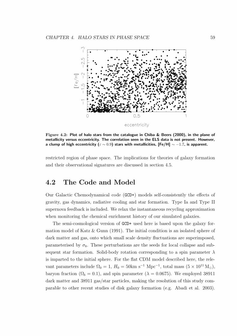
CHAPTER 4. HALO STARS IN PHASE SPACE 59
Figure 4.2: Plot of halo stars from the catalogue in Chiba & Beers (2000), in the plane ofmetallicity versus eccentricity. The correlation seen in the ELS data is not present. However,a clump of high eccentricity (ε ∼ 0.9) stars with metallicities, [Fe/H] ∼ −1.7, is apparent.
restricted region of phase space. The implications for theories of galaxy formation
and their observational signatures are discussed in section 4.5.
4.2 The Code and Model
Our Galactic Chemodynamical code (GCD+) models self-consistently the effects of
gravity, gas dynamics, radiative cooling and star formation. Type Ia and Type II
supernova feedback is included. We relax the instantaneous recycling approximation
when monitoring the chemical enrichment history of our simulated galaxies.
The semi-cosmological version of GCD+ used here is based upon the galaxy for-
mation model of Katz & Gunn (1991). The initial condition is an isolated sphere of
dark matter and gas, onto which small scale density fluctuations are superimposed,
parameterised by σ8. These perturbations are the seeds for local collapse and sub-
sequent star formation. Solid-body rotation corresponding to a spin parameter λ
is imparted to the initial sphere. For the flat CDM model described here, the rele-
vant parameters include Ω0 = 1, H0 = 50km s−1 Mpc−1, total mass (5× 10¹¹ M),
baryon fraction (Ωb = 0.1), and spin parameter (λ = 0.0675). We employed 38911
dark matter and 38911 gas/star particles, making the resolution of this study com-
parable to other recent studies of disk galaxy formation (e.g. Abadi et al. 2003).

CHAPTER 4. HALO STARS IN PHASE SPACE 60
The two models described here differ only in the value of σ8. In model 1, σ8 = 0.5,
as favoured in standard CDM (Ω0 = 1) cosmology. In model 2, we explore the use
of a smaller value for σ8 of 0.04, a value that results in a more rapid, dissipative,
collapse.
4.3 Simulation Results
Figure 4.3 illustrates the evolutionary histories of model 1, and figure 4.4 the evo-
lution of model 2, as density plots of star particles (panels with black backgrounds)
and gas particles (blue panels), with the redshift of each snapshot shown in its
respective star panel. Model 1 demonstrates classical hierarchical clustering - gas
collapses into the local dense regions seeded by the initial small-scale perturbation,
with star formation occurring subsequently in these over-dense regions. Stars con-
tinue to form in sub-clumps, as well as in the central region as a disk galaxy is built
up. We see less clumping in model 2, with gas streaming homogeneously toward the
centre of the galactic potential, resulting in most of the star formation occurring in
the central regions.
We analysed the bulk properties of our simulation at z = 0 and confirmed that
they were consistent with the simulations of Katz (1992), Steinmetz & Muller (1995),
Berczik (1999), and Bekki & Chiba (2001). The predicted surface density profiles,
metallicity gradients, specific angular momenta of gas and stars, and rotation curves
for our models did not differ significantly from previous studies, or between our own
two models. We suffer from the same classical overcooling problem encountered
in earlier studies (White & Frenk 1991). This results in excessive rates of star
production at early epochs, overly rapid metal enrichment, and a halo metallic-
ity distribution function peaked approximately one dex higher than that observed
(Ryan & Norris 1991). The field of metallicity distribution functions is the subject
of a future, lengthier, analysis, but we do note that this offset in the halo MDF peak
does not impact on our analysis here (as we can still adopt a differential metallicity
cut to delineate between the halo and thin disk in our simulation). We did find a
difference in the orbital eccentricity distribution of the simulated solar neighbour-
hood halo stars of the two models. After Bekki & Chiba (2000), individual stellar
eccentricities were calculated by allowing the orbits of star particles to evolve for
1.8 Gyrs under the gravitational potential of the simulated disk galaxy achieved at

CHAPTER 4. HALO STARS IN PHASE SPACE 61
Figure 4.3: X-Y stellar (black backgound) and gas (blue background) density plots of theevolution of model 1. The Z axis is defined to be the initial axis of rotation. Star panelsare labelled with redshifts, and appear below their corresponding gas panels. Hierarchicalclustering is evident in model 1. Gas collapses into local dense regions, and this is where starformation takes place.
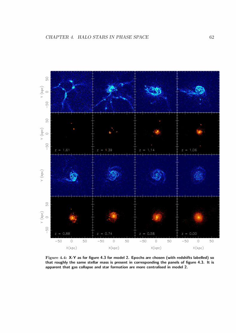
CHAPTER 4. HALO STARS IN PHASE SPACE 62
Figure 4.4: X-Y as for figure 4.3 for model 2. Epochs are chosen (with redshifts labelled) sothat roughly the same stellar mass is present in corresponding the panels of figure 4.3. It isapparent that gas collapse and star formation are more centralised in model 2.

CHAPTER 4. HALO STARS IN PHASE SPACE 63
Figure 4.5: Present-day eccentricity distribution of halo stars at the solar circle for our twomodels - the green line represents model 1, while the red line represents model 2. The blackline corresponds to the observational dataset of Chiba & Beers (2000). Model 1 leads to agreater number of high-eccentricity halo stars in the solar circle.
z = 0. Eccentricities ε were then derived using ε = (Rapo − Rperi)/(Rapo + Rperi),
where Rapo (Rperi) is the apogalactic (perigalactic) distance from the centre of the
simulated galaxy. Halo stars are defined to be simulated star particles with [Fe/H]
< −0.6. Due to the higher-than-expected absolute value for the halo MDF (alluded
to earlier), this metallicity cut may lead to an underestimate of the halo population,
but the final halo ”sample” is representative.
The green line of the histogram in figure 4.5 shows the eccentricity distribution
of halo star particles in the solar circle of model 1, with the red line representing
model 2. The solar circle is defined as an annulus of the galactic disk1, bounded
by 5 < RXY < 12 kpc and |Z| < 2 kpc, where Z corresponds to the rotation axis
and RXY =√
(X2 + Y2). Each bin shows the fraction of such star particles lying
in a given eccentricity range. Also shown (solid line) is the observational constraint
from CB00. Model 1 produced a greater number of high-eccentricity (ε > 0.8) solar
circle halo stars, and is in better agreement with observation.
Considering the analysis of ELS, whose rapid collapse model resulted in highly
eccentric halo stars, it was not unreasonable to expect that the more dissipative,
1The volume encompassed by our so-called ”solar neighbourhood” annulus is roughly an order-of-magnitude larger than the analog employed in the observational dataset by CB00. We haveensured that this apparent volume ”mismatch” does not impact upon our results by testing forsensitivity to azimuthal variations within the annulus through randomly subdividing the simulateddataset into random octiles. The effects described here in phase-space are robust to this azimuthalsubdivision.
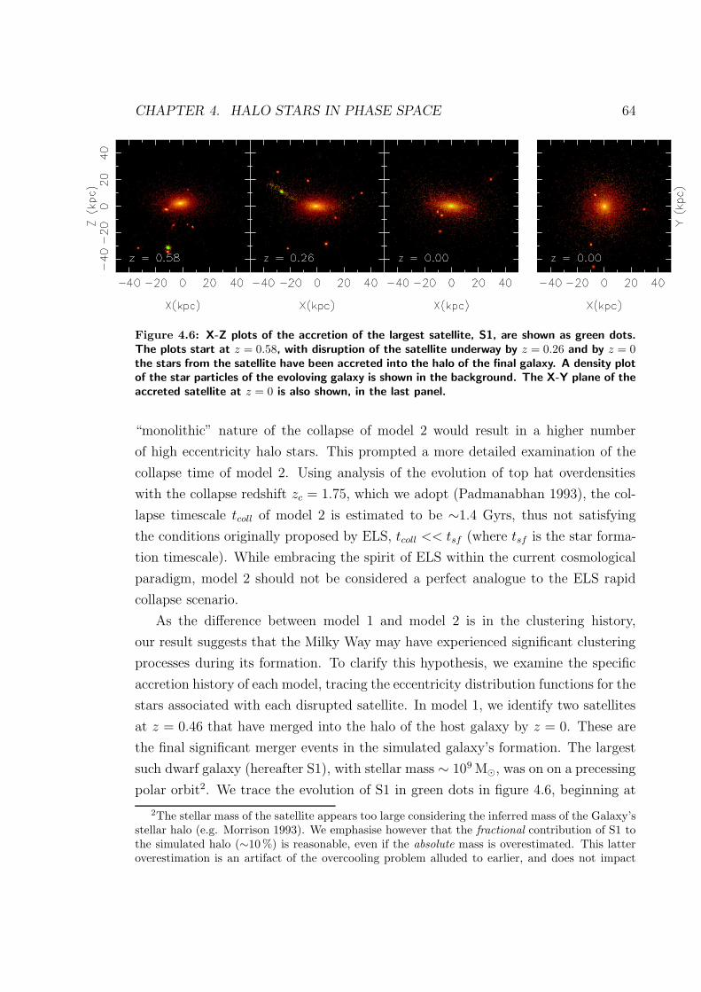
CHAPTER 4. HALO STARS IN PHASE SPACE 64
Figure 4.6: X-Z plots of the accretion of the largest satellite, S1, are shown as green dots.The plots start at z = 0.58, with disruption of the satellite underway by z = 0.26 and by z = 0the stars from the satellite have been accreted into the halo of the final galaxy. A density plotof the star particles of the evoloving galaxy is shown in the background. The X-Y plane of theaccreted satellite at z = 0 is also shown, in the last panel.
“monolithic” nature of the collapse of model 2 would result in a higher number
of high eccentricity halo stars. This prompted a more detailed examination of the
collapse time of model 2. Using analysis of the evolution of top hat overdensities
with the collapse redshift zc = 1.75, which we adopt (Padmanabhan 1993), the col-
lapse timescale tcoll of model 2 is estimated to be ∼1.4 Gyrs, thus not satisfying
the conditions originally proposed by ELS, tcoll << tsf (where tsf is the star forma-
tion timescale). While embracing the spirit of ELS within the current cosmological
paradigm, model 2 should not be considered a perfect analogue to the ELS rapid
collapse scenario.
As the difference between model 1 and model 2 is in the clustering history,
our result suggests that the Milky Way may have experienced significant clustering
processes during its formation. To clarify this hypothesis, we examine the specific
accretion history of each model, tracing the eccentricity distribution functions for the
stars associated with each disrupted satellite. In model 1, we identify two satellites
at z = 0.46 that have merged into the halo of the host galaxy by z = 0. These are
the final significant merger events in the simulated galaxy’s formation. The largest
such dwarf galaxy (hereafter S1), with stellar mass ∼ 109 M, was on on a precessing
polar orbit2. We trace the evolution of S1 in green dots in figure 4.6, beginning at
2The stellar mass of the satellite appears too large considering the inferred mass of the Galaxy’sstellar halo (e.g. Morrison 1993). We emphasise however that the fractional contribution of S1 tothe simulated halo (∼10 %) is reasonable, even if the absolute mass is overestimated. This latteroverestimation is an artifact of the overcooling problem alluded to earlier, and does not impact

CHAPTER 4. HALO STARS IN PHASE SPACE 65
Figure 4.7: As for figure 4.6, for a second satellite, S2, which is also accreted into the haloof the galaxy, Disruption for this satellite begins after z = 0.46, is well advanced by z = 0.26,and the satellite is accreted to the halo by z = 0. The stars from S2 end up in a slightly moreflattened distribution than the stars of S1.
z = 0.58, prior to disruption. By z = 0.26, tidal forces have begun stripping stars
from S1, and by z = 0, its stars are spread effectively throughout the halo. Accretion
of a second satellite, identifed as S2, is shown in figure 4.7. Again, it is evident that
stars from the satellite accrete predominantly to the halo of the galaxy.
The histogram of figure 4.8 shows the eccentricity distribution of solar circle
halo stars that originated in the satellites identified at z = 0.46, plotted with a red
line. The y-axis is normalised by the total number of solar circle halo stars in each
eccentricity bin. The green line is those stars from S1. We notice that the majority
of these halo stars are of high-eccentricity, and that S1 in particular contributes
∼20 % of all high-eccentricity halo stars in the solar circle at z = 0.
4.4 Phase Space Analysis
In figure 4.9, we plot the phase space distributions of solar circle stars of model 1.
Figures 4.9 a-c show: velocity directed radially away from the galactic center Vrad
versus rotational velocity in the plane of the disk Vφ; velocity out of the plane Vz
versus Vφ; and Vrad versus Vz. Figure 4.9 d plots the integrals of motion, projected
angular momentum Lz versus the absolute value of the energy (|E|). Stars originat-
ing in S1 are marked as open circles. We see that such stars occupy a restricted
region of phase space. It is worth noting that these results are qualitatively similar
upon the phase-space conclusions described here. Overcooling is a serious problem plaguing allchemodynamical codes, and is addressed in a more detailed paper to follow.
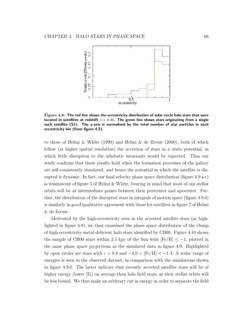
CHAPTER 4. HALO STARS IN PHASE SPACE 66
Figure 4.8: The red line shows the eccentricity distribution of solar circle halo stars that werelocated in satellites at redshift z = 0.46. The green line shows stars originating from a singlesuch satellite (S1). The y-axis is normalised by the total number of star particles in eacheccentricity bin (from figure 4.5).
to those of Helmi & White (1999) and Helmi & de Zeeuw (2000), both of which
follow (at higher spatial resolution) the accretion of stars in a static potential, in
which little disruption to the adiabatic invariants would be expected. Thus our
study confirms that these results hold when the formation processes of the galaxy
are self-consistently simulated, and hence the potential in which the satellite is dis-
rupted is dynamic. In fact, our final velocity phase space distribution (figure 4.9 a-c)
is reminiscent of figure 5 of Helmi & White, bearing in mind that most of our stellar
orbits will be at intermediate points between their pericenter and apocenter. Fur-
ther, the distribution of the disrupted stars in integrals of motion space (figure 4.9 d)
is similarly in good qualitative agreement with those for satellites in figure 7 of Helmi
& de Zeeuw.
Motivated by the high-eccentricity seen in the accreted satellite stars (as high-
lighted in figure 4.8), we then examined the phase space distribution of the clump
of high-eccentricity metal-deficient halo stars identified by CB00. Figure 4.10 shows
the sample of CB00 stars within 2.5 kpc of the Sun with [Fe/H] ≤ −1, plotted in
the same phase space projections as the simulated data in figure 4.9. Highlighted
by open circles are stars with ε > 0.8 and −2.0 < [Fe/H] < −1.4. A wider range of
energies is seen in the observed dataset, in comparison with the simulations shown
in figure 4.9 d. The latter indicate that recently accreted satellite stars will be of
higher energy (lower |E|) on average than halo field stars, as their stellar orbits will
be less bound. We thus make an arbitrary cut in energy in order to separate the field

CHAPTER 4. HALO STARS IN PHASE SPACE 67
Figure 4.9: (a)-(c): Velocity space (Vφ, Vrad, Vz) projections of the present-day solar circlestars of model 1. Open circles denote the subset of stars originating in S1. (d): The distributionfor the same stars in integrals of motion space - i.e., the absolute value of the total energy(|E|) versus projected angular momentum (Lz).

CHAPTER 4. HALO STARS IN PHASE SPACE 68
Figure 4.10: Velocity and integrals of motion phase space for the 729 Chiba & Beers (2000)stars within 2.5 kpc of the Sun with [Fe/H] <−1. (a)-(c): velocity space; (d): energy versusprojected angular momentum. Stars with eccentricity 0.8< ε < 1.0 and metallicity −2.0<[Fe/H] <−1.4 are represented as open circles. Solid black circles denote stars of high energy,while solid grey circles correspond to high energy stars with −800< Lz < 0 kpc km/s.

CHAPTER 4. HALO STARS IN PHASE SPACE 69
stars from those we suspect come from an accreted satellite, and the new subset of
stars are marked by solid circles. We notice immediately that these stars are more
tightly confined in phase space, and closely resemble the distribution of the accreted
satellite in our simulation.
4.5 Discussion
We have simulated self-consistently two models representing the formation of a Milky
Way-like galaxy using our N-body/SPH chemodynamical code GCD+. The models
differ only in the amplitude of small scale density perturbations σ8 incorporated
into the initial conditions. This results in different merging histories, which we then
use to search for distinctive present-day chemical and kinematical signatures of the
simulated galaxies’ early formation epochs. In model 1, stars form in local dense
regions of gas, seeded by a value of σ8 comparable to current CDM orthodoxy. The
galaxy subsequently builds up via a series of mergers in the manner of standard
hierarchical structure formation scenarios. A low value of σ8 in model 2 results in
a more dissipative collapse of the baryonic matter, with star formation occurring
predominantly in the galaxy’s central regions. Both models result in disk galaxies
with remarkably similar qualities; model 1, however, produces a greater number
of high-eccentricity halo stars, and in this regard is in better agreement with the
observational dataset of CB00. By tracing the merging histories of satellites in
model 1, it becomes apparent that a significant number of high-eccentricity halo stars
originate in accreted dwarf galaxies. In fact, almost 20 % of high-eccentricity halo
stars located in the solar circle originate in one satellite, of stellar mass ∼109 M,
which was on a precessing polar orbit and was accreted over the past ∼5 Gyrs.
Thus our simulation suggests that stars from an accreted satellite that was on a
polar orbit can constitute part of the galaxy’s halo, and that such stars have highly
eccentric orbits. Originating in accreted polar satellites, these stars would not gain
the angular momentum induced by the tidal torque of the external gravitational
field that results in the rotation of the disk component of the galaxy. Such stars
will fall toward the centre of the galactic potential and end up on highly eccentric
orbits.
The existence of an apparent correlation between metallicity and eccentricity in
halo stars was interpeted by ELS as a sign that rapid collapse drives the formation of

CHAPTER 4. HALO STARS IN PHASE SPACE 70
the Galaxy. Our study suggests that another way of creating such high-eccentricity
halo stars is through the recent accretion of polar orbit satellites. Furthermore, dwarf
galaxies of stellar mass ∼ 109 M typically have appropriate average metallicities
to be the source of this group of stars with [Fe/H] ∼ −1.7 (e.g. Mateo 1998).
Velocity phase space and the space of adiabatic invariants is where we would expect
substructure within the halo due to past merging to be apparent. The distribution in
such space of an accreted satellite of our simulated galaxy resembles that of previous
studies that traced the disruption of dwarf galaxies in static potentials, in particular
figure 5 of Helmi & White (1999). The greater dispersion in the distributions of our
simulation can most likely be attributed to the dynamic nature of the potential in
our full simulation of Galactic evolution, eroding the invariance of the integrals of
motion. The identified concentration of high-eccentricity, low-metallicity, halo stars
from CB00 occupy a very similar, restricted, region of phase space to the simulated
accreted satellite.
The possibility that this concentration of stars in the eccentricity-metallicity
plot is caused by satellite accretion was previously noted by Dinescu (2002). In
the metallicity range −2.0 < [Fe/H] < −1.5 of the CB00 data, Dinescu notes an
excess of stars in retrograde orbits with rotational velocity (Vφ) ∼ −30 km s−1,
from that expected from a “pure” halo. She identifies these stars as candidates for
having been torn from the system that once contained ω Cen. ω Cen is believed
to be the nucleus of a disrupted, accreted dwarf galaxy (e.g. Lee et al. 1999;
Majewski et al. 2000), is in a retrograde orbit, and has an orbital eccentricity of
∼0.67. Using a simple disruption model, Dinescu showed that the tidal streams
tend to have higher orbital eccentricity than the disrupted satellite. Along with the
mean metallicity of ω Cen being [Fe/H] = −1.6, the inference is that the clump of
high-eccentricity halo stars identified in CB00 contains a significant number of stars
which have been tidally stripped from ω Cen. Our simulations provide a degree of
support for this hypothesis. Taking only those stars with Lz < 0 in figure 4.10 d,
we see a clump of stars with intermediate energies and Lz ∼ −400 kpc km s−1.
These stars are identified in all phase space plots by black circles; we see that the
distribution becomes more restricted in each velocity space dimension, and there
is greater concordance with Helmi & White’s (1999) idealized satellite accretion
studies.
The key question we wish to address remains ... what are the implications for
the competing galaxy formation paradigms? A brief response is as follows: CB00

CHAPTER 4. HALO STARS IN PHASE SPACE 71
observed no correlation between eccentricity and metallicity for halo stars near the
Sun, obviating the need for a “rapid collapse” picture of the formation of the Galaxy
(ELS). However, CB00 do interpret a clump of high-eccentricity low-metallicity
([Fe/H]∼−1.7) stars in their dataset in terms of ELS - i.e. as a relic of a rapid
collapse phase. Our simulations suggest that an equally plausible origin for this
population is the recent accretion of a polar orbit satellite in the Galactic halo.
Chapter 5
Stellar Halo Constraints on
Simulated Late-Type Galaxies
5.1 Introduction
Formation scenarios for the Milky Way have been dominated by two canonical mod-
els: the rapid collapse of a proto-galactic cloud (Eggen, Lynden-Bell & Sandage
1962), and the hierarchical build up from low mass fragments (Searle & Zinn 1978).
Burkert (2001) reviews evidence that the early dissociation of gas from dark matter
in the first stages of the hierarchical build-up allows these two models to be com-
bined into one consistent formation scenario. In this scenario, the Galactic spheroid
is formed by hierarchical merging of substructures, while the disk components result
from the smooth infall of diffuse gas. This picture is consistent with the predictions
of classical cold dark matter (CDM) scenarios (White & Frenk 1991; Kauffmann
et al. 1993)
Simulations now show that the observed large scale properties of galaxies can
be reproduced within CDM cosmological models. For example, Steinmetz & Muller
(1995) studied the chemo-dynamical evolution of disk galaxies, and succeeded in
distinguishing the chemical properties between halo, disk and bulge stars. Raiteri,
Villata, & Navarro (1996) and Berczik (1999), reproduced the correlation between
[O/Fe] and [Fe/H] of solar neighbourhood stars by tracing the metal enrichment
by Supernovae Type II (SNe II) and Type 1a (SNe Ia). Steinmetz & Navarro
(1999), Navarro & Steinmetz (2000), and Koda, Sofue, & Wada (2000) discussed
the zero point of the Tully-Fisher relationship by analysing the end products of
72
CHAPTER 5. CONSTRAINTS ON SIMULATED LATE-TYPE GALAXIES 73
their chemical evolution and stellar population synthesis models. The observed
eccentricity-metallicity relation of Milky Way halo stars has also been successfully
reproduced (Bekki & Chiba 2000; Brook et al. 2003).
However, several problems continue to plague these simulations. Notoriously,
the resulting structures are deficient in angular momentum (e.g. Navarro, Frenk &
White 1995). The simulations also fail to create galaxies in which most baryonic
matter resides in the thin disk, as observed in the Milky Way. Typically, these
simulations result in a stellar halo which is as massive or more massive than the
stellar disk. For example, in a recent high resolution study, Abadi et al. (2003)
create a galaxy with a stellar halo which contains over 60% of the total stellar mass
of the system, and a thin disk which constitutes only 17 % of the stellar mass, more
akin to an S0 than a late type disk galaxy. Such massive stellar halos inevitably
have a greater metallicity than observed in late type spirals. This leaves open the
question of the formation processes which lead to late type disk galaxies such as the
Milky Way, within the context of hierarchical structure formation scenarios.
It has long been postulated that energy feedback from SNe is necessary to solve
many of the above problems. Unfortunately, energy feedback from SNe explosions
remains one of the most difficult processes to model in galaxy formation simulations,
largely because feedback occurs on sub-resolution scales. A number of different SNe
feedback implementations have been employed in chemo-dynamical codes; for a
survey of such methods, see Thacker & Couchman (2000, TC hereafter).
Katz (1992) smooths thermal energy into nearest neigbour gas particles using the
smoothed particle hydrodynamic (SPH) kernel. This feedback scheme is known to
be largely inefficient, as the characteristic timescale of radiative cooling in the high
density regions, where star formation typically occurs, is shorter than the dynamical
timescale. Navarro & White (1993) extend this technique to include both thermal
and kinetic energy. A parameter, f, controls the fraction of energy input as kinetic
as opposed to thermal energy. Although f and the total amount of energy both may
vary, this feedback scheme is common to many galaxy formation simulations (e.g.
Steinmetz & Navarro 2002; Kobayashi 2002; Nakasato & Nomoto 2003; Abadi et al.
2003). Representations of the multi-phase interstellar medium are made by Hultman
and Pharasyn (1999) and by Springel & Hernquist (2003), but these studies are
limited by the dynamical dependence of the two phases. In Gerritsen (1997), energy
is returned by heating an individual SPH particle, a technique that is successful
for simulating dwarf size systems. TC and Kay et al. (2002) examine a scheme in
CHAPTER 5. CONSTRAINTS ON SIMULATED LATE-TYPE GALAXIES 74
which the feedback region is adiabatic. Such a feedback scheme was shown to be
more effective in an isolated, dwarf type galaxy than in a MilkyWay-sized galaxy.
In this study, we examine the link between the energy feedback and the prop-
erties of the final galaxy; specifically the halo/disk stellar mass ratio and the halo
metallicity distribution function (MDF). We demonstrate the importance of feed-
back in regulating star formation in the small systems that collapse at early epochs
of galaxy evolution. In section 5.2, details of our chemo-dynamical code, GCD+, and
our two models incorporating different feedback schemes are provided. We examine
and compare the properties of the two simulated galaxies in section 5.3, concentrat-
ing on the halo/disk stellar mass ratio and the halo MDFs of the simulated disk
galaxies. One feedback model results in a galaxy which is a better representation
of a late type galaxy than the other. In section 5.4, we trace the baryons that form
the disk of the galaxies, highlighting the processes that lead to the difference in
the fraction of stars ending up in the disk rather than the halo. The discussion in
section 5.5 summarises the contribution of this study to our understanding of how
thin disks form from structures within CDM cosmologies.
5.2 The Code and Model
Our Galactic chemo-dynamical code, GCD+, self-consistently models the effects of
gravity, gas dynamics, radiative cooling and star formation. We include SNe II and
SNe Ia feedback, and avoid use of the instantaneous recycling approximation in
modelling the chemical enrichment. Details of GCD+ can be found in chapter 2. We
describe here only the details concerning the inclusion of SNe energy feedback.
We assume that 1051ergs is fed back as thermal energy from each SNe. In our
thermal feedback model, denoted “TFM” hereafter, energy from SNe II and SN Ia is
smoothed over surrounding gas particles according to the SPH kernel, in the form
of thermal energy (following Katz 1992).
Our second model incorporates a different feedback mechanism for SNe II. These
SNe trace starburst regions, and are therefore more susceptible to the inefficiency of
the feedback algorithms used in the TFM. In our adiabatic feedback model, “AFM”
hereafter, gas within the SPH smoothing kernel of SNe II explosions is prevented
from cooling. This adiabatic phase is assumed to last for the lifetime of the lowest
mass star which ends as a SNe II, i.e. the lifetime of an 8 M star (∼100 Myr). In

CHAPTER 5. CONSTRAINTS ON SIMULATED LATE-TYPE GALAXIES 75
Figure 5.1: Density plots for TFM (top) and AFM at z=0. Stars and gas are shown face-on(X-Y plane) and edge-on (X-Z). In the TFM, a thin disk is evident in the gas distribution, butthe galaxy’s stellar mass is dominated by halo stars, and resembles an S0 galaxy. In the AFM,the galaxy is dominated by a thin stellar disk. A large gaseous thin disk, still undergoing starformation, has also formed.
the AFM, the energy released by SNe Ia, which do not trace starburst regions, is
fed back as thermal energy. The AFM is similar to a model presented in TC.
We use semi-cosmological simulations that are based upon the galaxy forma-
tion model of Katz & Gunn (1991). The initial condition is an isolated sphere
of dark matter and gas, onto which small scale density fluctuations are superim-
posed, parameterised by σ8. These perturbations are the seeds for local collapse
and subsequent star formation. Solid-body rotation corresponding to a spin param-
eter, λ≡J |E|1/2/GM5/2tot , is imparted to the initial sphere, where J , E and Mtot are
the total angular momentum, energy, and mass of the system respectively. Rel-
evant parameters include the total mass (5×10¹¹ M), baryon fraction (Ωb=0.1),
spin parameter (λ=0.0675) and σ8=0.5. We employed 38911 dark matter and 38911
gas/star particles, making the resolution of this study comparable to other recent
studies of disk galaxy formation (e.g. Abadi et al. 2003).
We again emphasise that the two models analysed here are identical, except in
the way in which the energy from SNe II affects the surrounding gas.

CHAPTER 5. CONSTRAINTS ON SIMULATED LATE-TYPE GALAXIES 76
Figure 5.2: Global star formation rate (SFR) as a function of lookback time for the twosupernova energy feedback models applied to the same CDM overdensity. Inefficient feedbackof the TFM results in high SFR at early times compared to the AFM.
5.3 Results
Figure 5.1 shows a density plot of the final stellar and gaseous components of the
two models. Both simulations result in flattened stellar structures and thin gaseous
disks. In the TFM, the stellar mass is dominated by halo stars, and a thin disk is
evident in the gas distribution. The final galaxy more closely resembles an S0 galaxy
than a late type spiral. Star formation is rapid during early epochs (figure 5.2), as a
result of the inefficiency of the feedback. The peaks in the star formation rates are
related to early major merger episodes. Star formation continues at a steady rate,
primarily in the disk, over the last ∼7 Grys, a relatively quiescent period with only
a few minor merger events.
It is clear from the edge on view of the stellar populations in figure 5.1 that
the AFM has created a more dominant stellar disk. Star formation in the AFM
is suppressed at early epochs (figure 5.2) compared to the TFM. The signatures of
the early mergers of the TFM are also evident in the AFM star formation peaks, a
result of the identical initial conditions. The greater availability of gas means the
AFM creates more stars at later times than the TFM: ∼1.9×10¹⁰M compred with
∼8.2×10⁹ M in the last 8 Gyrs. The result is the creation of a more dominant
stellar disk. A large gaseous thin disk, still undergoing star formation, has also
formed. The mass of cold gas (T<4×10⁵K) associated with the disk is larger for the
AFM, ∼9×10⁹ M than for the TFM, ∼5×10⁹ M.

CHAPTER 5. CONSTRAINTS ON SIMULATED LATE-TYPE GALAXIES 77
Figure 5.3: Halo metallicity distributions for the TFM (red line) and AFM (blue line), givingthe relative fraction of halo stars within a given metallicity bin. Halo stars are defined byweighting star particles by mass within the regions 4<R<50 kpc and |Z|>4 kpc.
In this study, we focus on the mass and metallicities of the stellar halos of our
simulated galaxies. Halo stars are defined spatially using two hemispheres defined
by 4<R<50 kpc and |Z|>4 kpc. The density gradient in shells of these hemispheres
is integrated over the sphere out to 50 kpc to find the mass of the stellar halo.
Disk stars are defined by the distribution of specific angular momentum (Lzs) as
a function of specific binding energy(Es). It is clear from figure 5.1 that the gas
particles are predominantly in a disk, resulting in their confinement to a small
region in Lzs vs. Es space. This same region is used to define simulation disk stars;
cuts in the Z components of velocity (|VZ |<65 km/s) and position (|Z|<1 kpc) have
also been imposed.
The stellar population of the TFM is dominated by halo stars; indeed, the stellar
halo is a factor of 1.2 times more massive than its stellar disk population. The AFM
has a halo/disk mass fraction ∼6 times smaller, more closely resembling a late type
galaxy. Nevertheless, this fraction is still almost an order of magnitude larger than
the halo/disk ratio of the Milky Way. The large mass of the stellar halo in the
TFM is intimately linked to its high metallicity, as seen in figure 5.3. The peak of
the halo MDF has shifted from [Fe/H]∼0 for the TFM (red line), to [Fe/H]∼−1.0
for the AFM (blue line), a full factor of ten in metallicity. The peak of the halo
MDF in the AFM is somewhat higher than that of the Milky Way halo MDF, which

CHAPTER 5. CONSTRAINTS ON SIMULATED LATE-TYPE GALAXIES 78
peaks at [Fe/H]∼−1.5 (Ryan & Norris 1991), but is lower than the peak for M31,
[Fe/H]∼−0.7 (Durrell et al. 1994). These results suggest that strong feedback from
SNe is important for the formation of the stellar halos of disk galaxies.
Recently, significant progress has been made on the theoretical and observational
signatures of satellite accretion in present day stellar populations, e.g. Helmi &
White 2000; Bekki & Chiba 2001; Brook et al. 2003. Moreover, the model used
in TC that incorporated adiabatic feedback was shown to have a greater effect on
smaller systems. Thus, the subclumps of the simulation were a natural place to
search for the formation processes responsible for the different galaxy properties
produced by the different models.
In figures 5.4-5.11, we show the disruption process for two typical satellites from
each of the TFM and the AFM. Red particles are stars present in the satellite prior
to any disruption. Gas particles are green. Star particles formed after the disruption
process begins are blue. A grey scale density plot of the simulation stars is in the
background. There are ∼1000 baryon particles in each satellite, corresponding to
∼109 M. Six time-steps are shown, both face-on and edge-on, for these typical
merging events.
The disruption of one satellite in the TFM, TS1, is shown in the panels of
figures 5.4-5.5. The satellite begins as a dense, stellar dominated system. This is a
result of rapid early star formtion, between 11 and 8 Gyrs ago (figure 5.12 red line).
By 4.7 Gyrs ago, the satellite is disrupted and star formation has ceased within the
dwarf. By 3.6 Gyrs ago, accretion is well underway. Due to their collisionless nature,
the accreted stars spread throughout the halo by z=0. Gas from the satellite falls
to the disk region of the host galaxy, where new stars (blue) are born. The amount
of gas falling into the disk region, and forming stars, is small as most gas has been
exhausted before the satellite merged. The disruption of a second satellite in the
TFM, TS2, is also shown in the panels of figures 5.6-5.7. TS2 is accreted at an
ealier time than TS1, with disruption well under way by 6.7 Gyrs ago. Again, the
star formation rate is high at early epochs (figure 5.13 red line), and stars accrete
predominantly to the halo of the galaxy.
In satellite AS1 from the AFM, star formation in the subclumps is regulated
(figure 5.12, blue line) prior to disruption. Gas remains less densely concentrated
than stars and is preferentially stripped. This pre-enriched gas dissociates from the
dark matter, and accretes smoothly on to the disk region. On the other hand, stars
from the satellite are accreted into the halo of the galaxy by z=0. Therefore, the
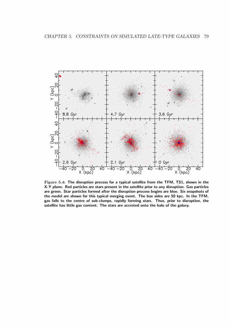
CHAPTER 5. CONSTRAINTS ON SIMULATED LATE-TYPE GALAXIES 79
Figure 5.4: The disruption process for a typical satellite from the TFM, TS1, shown in theX-Y plane. Red particles are stars present in the satellite prior to any disruption. Gas particlesare green. Star particles formed after the disruption process begins are blue. Six snapshots ofthe model are shown for this typical merging event. The box sides are 50 kpc. In the TFM,gas falls to the centre of sub-clumps, rapidly forming stars. Thus, prior to disruption, thesatellite has little gas content. The stars are accreted onto the halo of the galaxy.

CHAPTER 5. CONSTRAINTS ON SIMULATED LATE-TYPE GALAXIES 80
Figure 5.5: The disruption of TS1 shown in the X-Z plane. All other details as in figure 5.4.From side-on, it is apparent that old stars accrete to the stellar halo of the simulated galaxy.

CHAPTER 5. CONSTRAINTS ON SIMULATED LATE-TYPE GALAXIES 81
Figure 5.6: Same as figure 5.4, for the accretion of a second satellite, TS2, in the TFM.Again we see a satellite with little gas, whose stars are accreted predominantly into the galactichalo. Stars born after the disruption of the satellite begins (blue) are more centralised thanold stars (red).
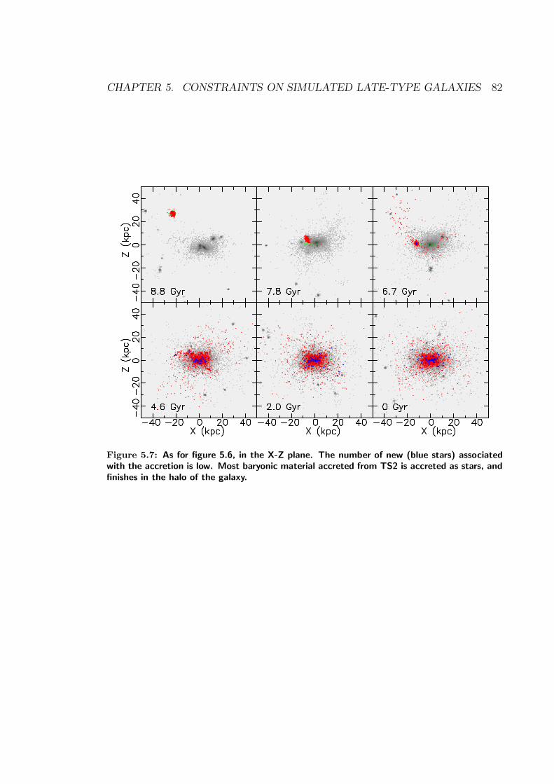
CHAPTER 5. CONSTRAINTS ON SIMULATED LATE-TYPE GALAXIES 82
Figure 5.7: As for figure 5.6, in the X-Z plane. The number of new (blue stars) associatedwith the accretion is low. Most baryonic material accreted from TS2 is accreted as stars, andfinishes in the halo of the galaxy.

CHAPTER 5. CONSTRAINTS ON SIMULATED LATE-TYPE GALAXIES 83
Figure 5.8: The disruption process for a typical satellite, AS1, from the AFM. Red particlesare stars present in the satellite prior to any disruption. Gas particles are green. Star particlesformed after the disruption process begins are blue. Four edge-on snapshots of the modelare shown for this typical merging event. In the AFM, gas remains less densely concentratedthan stars and is preferentially stripped, decoupling from the dark matter. The stripped gasaccretes smoothly to the disk region. Stars from the satellite are accreted into the halo of thegalaxy by z=0. Pre-enriched gas stripped from the satellites feeds the thin disk, where newstars (blue) are born over the past ∼8 Gyrs.

CHAPTER 5. CONSTRAINTS ON SIMULATED LATE-TYPE GALAXIES 84
Figure 5.9: As for figure 5.8, in the X-Z plane. It is clear in this plane that gas (greenparticles) accreted from AS1 falls to the disk, where new stars (blue) are born, whereas starsaccreted from the satellite end up in the galactic halo.

CHAPTER 5. CONSTRAINTS ON SIMULATED LATE-TYPE GALAXIES 85
Figure 5.10: As for figure 5.8, for a second satellite, AS2, from the AFM. Again the effectof gas remaining less densely concentrated than stars is apparent, and stripped gas accretessmoothly to the disk region. Stars from the satellite are accreted into the halo of the galaxyby z=0. New stars (blue) are born in the disk over the past ∼8 Gyrs.

CHAPTER 5. CONSTRAINTS ON SIMULATED LATE-TYPE GALAXIES 86
Figure 5.11: The satellite in figure 5.10, shown in the X-Z plane. Again it is evident thatstars present as accretion begins (red particles) end up in the halo of the galaxy. The edge-onview makes it clear that gas (green particles) accretes to the disk where new stars (blue) areborn.

CHAPTER 5. CONSTRAINTS ON SIMULATED LATE-TYPE GALAXIES 87
Figure 5.12: Total star formation rates (SFR) within the satellite systems TS1 of the TFM(red line), seen in figures 5.4-5.5, and AS1 from the AFM (blue line), seen in figures 5.8-5.9. As in the host galaxy, star formation is early and rapid in the satellite TS1 of the TFM,compared to the star formation in satellite AS1 of the AFM.
stars that end up in the halo are the oldest stars formed in the subclumps, as well
as the most metal poor, as chemical enrichment has been suppressed in these small
systems by the strong feedback in the AFM. Disruption of a second, more massive
satellite (∼ 2×10⁹ M), AS2 from the AFM is also shown, with regulated early star
formation (figure 5.13, blue line), and gas accreting to the disk region where new
stars are born.
The accretion events shown in this section occur at intermediate age in the
galaxy formation process. They do not demonstrate that late accreting satellites
are the source of all disk and halo material. Rather, they evince the effectiveness
of SNe feedback on satellites. AFM also leads to regulated star formation in the
smaller systems that have collapsed at high redshift, as is clear from figure 5.2.
In a CDM cosmology, the stellar halo is likely to be built up by the accretion of
a significant number of such small systems, including tidally-stripped stars during
multiple mergers of building blocks at high redshift (Bekki & Chiba 2001). Our
results demonstrate that the AFM produces enough SNe energy to suppress star
formation and chemical enrichment in the building blocks of galaxy formation, and
that this leads to a less massive, more metal poor, stellar halo that is in better
agreement with observation.

CHAPTER 5. CONSTRAINTS ON SIMULATED LATE-TYPE GALAXIES 88
Figure 5.13: Total star formation rates (SFR) within the satellite systems TS2 of the TFM(red line), seen in figures 5.6-5.7, and AS2 from the AFM (blue line), seen in figures 5.10-5.11.Again, star formation is early and rapid in the satellite TS2 of the TFM compared to AS2 ofthe AFM.
5.4 Discussion
Energy feedback has emerged as a possible solution to several of the problems that
plague models of the formation of late type disk galaxies in CDM scenarios. Despite
this recognition, the manner in which feedback is incorporated into SPH codes re-
mains problematic. In this study we have been concerned primarily with the effects
of feedback on the mass and metallicity distribution of the stellar halos of simulated
galaxies, and its capacity to regulate star formation in high-redshift galactic building
blocks.
We implement two different feedback schemes into a seed galaxy with the same
initial perturbation. Incorporating thermal feedback similar to that of Katz (1992)
results in a flattened, disk-like galaxy that resembles those of previous studies (e.g.
Steinmetz & Mullar 1995; Berzcik 1999; Abadi et al. 2003). The fundamental
problem is that the ratio of the mass of the halo and disk components is much too
high and the metallicity of the halo component is also too high in comparison to
the observations of the Millky Way; in both cases by about a factor of 10. There is
less conflict with observations of M31. In the TFM, the gas cools to the centre of
building blocks, rapidly forming stars (figure 5.2). The rapid star formation cycles
also result in metallicities that quickly approach solar levels and more stars with
high metallicity. Due to the collisionless nature of the stellar component, these stars

CHAPTER 5. CONSTRAINTS ON SIMULATED LATE-TYPE GALAXIES 89
end up in the halo of the host galaxy after tidal disruption. The halo thus becomes
very massive and very metal rich.
With the AFM, gas is delayed from cooling in star burst regions. Star formation
is regulated in small systems, such as building blocks, and lower fractions of the
initial baryonic content of these building blocks are converted to stars. These build-
ing blocks thus have lower metallicity stars and a hotter, more diffuse gas content,
allowing gas to be dissociated from the collapsing dark matter that drives structure
formation. During the tidal disruption of these building blocks, the gas is prefer-
entially stripped and, due to its dissipative nature, accretes smoothly onto the thin
disk; this pre-enrichment helps in alleviating the G-dwarf problem (Fenner & Gibson
2003). The stars that are formed in these building blocks are accreted preferentially
into the halo of the galaxy. As a smaller fraction of baryons are turned into star
particles in the building blocks in the AFM, the halo of the resulting host galaxy is
less massive and more metal poor. Also, even if they are accreted into the galaxy at
a later epoch than the gas, the stars stripped from these building blocks are older
than the stars that subsequently form in situ in the thin disk: halo stars are old and
metal poor, disk stars are new and metal rich. The result is a disk galaxy that is a
far better realisation of the Milky Way and M31, compared to the canonical TFM.
Besides observations of the Milky Way’s stellar halo mass and MDF, which have
been the main focus of this paper, additional Local Group observations provide a
measure of support for the processes outlined here. The Magellanic Stream is con-
sistent with the suggestion that gas is preferentially stripped from accreting satellite
galaxies (Putman et al. 1998). The Sagittarius Dwarf and Sagittarius stream are
totally stellar (Koribalski et al. 1994; Burton & Lockman 1999), suggesting that
this accreted satellite had previously lost its gas. The fact that Local Group dwarf
spheroidals are gas poor, and preferentially closer to the centre of the Milky Way
than gas rich dwarf irregulars provides further evidence, albeit circumstantial, that
gas from satellites is stripped prior to stellar accretion (van den Bergh 1999).
At this point, we note that we tested several other techniques in an attempt to
reproduce a halo mass and MDF closer to those observed in the Milky Way. These
included varying the star formation efficiency, adjusting the amount of feedback in-
corporated as kinetic energy, and implementing “re-ionisation epochs” during which
radiative cooling was essentially “squelched”(Somerville 2002). None of these adjust-
ments were successful in lowering the mass and metallicity of the simulated stellar
halo. To date, only the AFM has succeeded in lowering the metallicity and mass
CHAPTER 5. CONSTRAINTS ON SIMULATED LATE-TYPE GALAXIES 90
of the simulated galaxies’ stellar halos significantly. We believe that the observed
properties of the stellar halo provide strong constraints on disk galaxy formation
models, and suggest that many previous studies have inevitably failed to reproduce
these properties. The success of the AFM lies in two features: its ability to regulate
star formation at early epochs (figure 5.2), and the fact that its effect is more pro-
nounced in smaller systems (the early collapsing subclumps and later-forming dwarf
galaxies) than in a Milky Way-sized system.
Our simulations emphasise that it is critical for disk galaxy formation in a CDM
context that building blocks and later-accreting satellites be gas dominant. We
regard our simulations as a successful realistion of the scenario sketched by Burkert
(2001), which emphasised the need for an early phase of gas heating and dissociation
from dark matter in forming the Milky Way within hierarchical cosmologies.

Chapter 6
The Emergence of the Thick Disk
in a CDM Universe
6.1 Introduction
Since its existence was detected through star counts by Gilmore & Reid (1983), the
thick disk has become established as a component of the Milky Way that is distinct
from the thin disk. It is hoped that the old age of the stars associated with the
thick disk of the Milky Way will allow it to serve as a fossil record of the formation
processes of the early parts of Galactic evolution.
Several large surveys have been undertaken to constrain the properties of the
Milky Way’s thick disk. The local density of thick disk stars is about 6-13% of
that of the thin disk (e.g. Chen et al. 2001); the thick disk has a scale height
of 0.6-1 kpc (e.g. Phelps et al. 1999, Ojha 2000, Chen et al. 2001), about three
times larger than the thin disk; its stars are old, almost exclusively older than
12 Gyrs (e.g. Gilmore & Wyse 1985; Edvardsson et al. 1993; Fuhrmann 1998).
Thick disk stars have a wide range of metallicity, −2.2 ≤[Fe/H]≤ −0.5, (Chiba
& Beers 2000, hereafter CB), although the metal weak ([Fe/H]< −1.0) tail of the
distribution contributes only ∼1 % of the thick disk (Martin & Morrison 1998),
and may be a different population to the canonical thick disk (Beers et al. 2002).
We also note that Feltzing, Bensby & Lundstrom (2003, hereafter FBL) find that
the thick disk metallicity distribution extends to metallicities higher than [Fe/H]=
−0.5. The metallicity distribution peaks at [Fe/H]∼ −0.6 (Gilmore & Wyse 1985;
Wyse & Gilmore 1995; CB). Thick disk stars are also characterised by their warm
91

CHAPTER 6. THICK DISK FORMATION IN A CDM UNIVERSE 92
kinematics and a rotation that lags behind the thin disk, e.g. Stromgren (1987)
finds (σU ,σV ,σW )=(65,54,38)km/s, Vlag ∼40 km/s.
There is mounting evidence that the chemical trends in the thick and thin disk
stars are different (Fuhrmann 1998; Prochaska et al. 2000; Tautvaisiene et al. 2001;
Schroder & Pagel 2003; Mashokina et al. 2003, hereafter MGTB; Reddy et al. 2003;
FBL; also see Chen et al. 2000 for an alternative view). An important diagnostic
derived from this divergence the α-element to iron abundance ratio, which indicates
different formation timescales for the thin and thick disk. The enhanced α-element
abundances (compared to iron) that are observed in thick disk stars indicate a
short formation timescale in which enrichment is dominated by Type II supernovae
(SNe II). Although FBL found evidence of Type Ia supernovae (SNe Ia) enrichment
in the most metal rich of the thick disk stars, their values for [α/Fe] are systemati-
cally higher than thin disk stars with the same [Fe/H]. Fuhrmann (1998), Gratton
et al. (2000), and Mashonkina & Gehren (2001) conclude that star formation in the
thick disk lasted less than 1 Gyr, while correlations of various chemical elements in
thick disk stars lead MGTB to estimate this time scale to be ∼0.5 Gyrs. MGTB
also conclude that the homogeneity of abundances of thick disk stars indicates that
it formed from well-mixed gas, a conclusion that is consistent with the results of
Nissen & Schuster (1997), Fuhrmann (1998), and Gratton et al. (2000).
Over the past decade, N-body cosmological simulations have been successful in
reproducing many properties of disk galaxies. Employing a new implementation of
SNe feedback, Brook et al. (2003, BKGF hereafter) recently simulated a realistic disk
galaxy with a stellar mass dominated by a young stellar disk component, surrounded
by a less massive, old, metal poor, stellar halo. In this chapter, we examine this
simulated disk galaxy for evidence of a thick disk component, searching for clues as
to the origins of the thick disk within the hierarchical galaxy formation of a CDM
context.
In section 6.2, we outline details of our N-body chemo-dynamical evolution code,
GCD+, and the semi-cosmological galaxy formation model that we invoke. Initial con-
ditions are chosen that lead to the formation of a late type galaxy, whose properties
are presented in section 6.3. Further study of our simulated galaxy provides evidence
for the existence of a distinct thick disk population, similar to that of the Milky Way.
This allows us, in section 6.4, to trace the major thick disk formation epoch and
propose a thick disk formation scenario. In section 6.5 we compare our scenario to
other theories of thick disk formation, and discuss how current observational data
CHAPTER 6. THICK DISK FORMATION IN A CDM UNIVERSE 93
may discriminate between these theories.
6.2 The Code and Model
This chapter analyses data from the simulated late type galaxy of the Adiabatic
Feedback Model from BKGF. We briefly review some features of the code and model.
Our galactic chemo-dynamical evolution code, GCD+, self-consistently models the
effects of gravity, gas dynamics, radiative cooling, and star formation. We include
SNe Ia and SNe II feedback, tracing the lifetimes of individual stars, which enables
us to monitor the chemical enrichment history of our simulated galaxies. Details of
GCD+ can be found in Kawata & Gibson (2003).
We assume that 1051 ergs is fed back as thermal energy from each SNe. The
energy released by SNe is fed back as thermal energy, and smoothed over the nearest
neighbour gas particles according to the SPH kernel. This feedback scheme is known
to be inefficient (Katz 1992). To address this problem, gas within the SPH smoothing
kernel of SNe II explosions is prevented from cooling, creating an adiabatic phase
for gas heated by such SNe. This is similar to a model presented in Thacker &
Couchman (2000).
The semi-cosmological version of GCD+ used in this study is based upon the
galaxy formation model of Katz & Gunn (1991). The initial condition is an isolated
sphere of dark matter and gas. The top-hat overdensity has an amplitude, δi,
at initial redshift, zi, which is approximately related to the collapse redshift, zc,
by zc = 0.36δi(1 + zi) − 1 (e.g. Padmanabhan 1993). We set zc = 1.8, which
determines δi at zi = 40. Small scale density fluctuations are superimposed on the
sphere, parameterised by σ8. These perturbations are the seeds for local collapse and
subsequent star formation. Solid-body rotation corresponding to a spin parameter,
λ, is imparted to the initial sphere to incorporate the effects of longer wavelength
fluctuations. A large value of λ is chosen along with initial conditions in which
no major merger occurs in late epochs (z <1), in order to ensure a disk galaxy is
formed. For the model described here, the relevant parameters include the total
mass, 5 × 10¹¹ M, baryon fraction, Ωb = 0.1, star formation efficiency, c∗ = 0.05,
spin parameter, λ = 0.0675 and σ8 = 0.5. We employed 38911 dark matter and
38911 gas/star particles, making the resolution of this study comparable to other
recent studies of disk galaxy formation (e.g. Abadi et al. 2003).

CHAPTER 6. THICK DISK FORMATION IN A CDM UNIVERSE 94
Figure 6.1: z=0 density plots for stars and gas in both the X-Y (face on) and X-Z (edge on)planes. The galaxy is dominated by a stellar disk. A large gaseous thin disk, still undergoingstar formation, has also formed.
6.3 Properties of Final Galaxies
Figure 6.1 shows a density plot of the final stellar and gas populations of the simu-
lated galaxy, viewed face-on and edge-on. The stellar mass is dominated by a young
disk component. A large gaseous thin disk, still undergoing star formation, has also
formed. The stellar population of the low mass stellar halo component is old and
metal poor. The star formation history is shown in figure 6.2, which plots look-back
time against the star formation rate (SFR). The SFR peaks ∼9 Gyrs ago. The SFR
then declines over the next 4-5 Gyrs, but is reasonably steady over the last ∼5 Gyrs.
For this study, we are interested in the thick disk component. In observations
of the Milky Way, the peculiar velocity of stars is a useful diagnostic to distinguish
thick disk stars from thin disk stars. For observed solar neighbourhood stars, it
is well established that there is a relationship between velocity dispersion and age.
Figure 6.3 shows the observed relation as grey symbols, with error bars, as read
from figure 3 of Quillen & Garnett (2001), who use the data of Edvardsson et al.
(1993). The velocity dispersion data plateau between the ages of ∼10 and 2 Gyrs;
these stars belong to the old thin disk. A slight decrease in dispersion is apparent
for star particles less than ∼2 Gyrs old. Notably, the velocity dispersions increase
abruptly, approximately doubling, ∼10 Gyrs ago. These older stars belong to the
thick disk1. In figure 6.3 we use “+” symbols to plot the relation between the three
components of the velocity dispersion, and the stellar age, for solar neighbourhood
star particles in our simulation. The solar neighbourhood is defined as the annulus
1We note that a more recent study by Nordstrom et al. (2004) revisits this relation, and findsthat the thin disk stars do show a slight increase of velocity dispersion with age, but stars olderthan ∼10 Gyrs were excluded from their study.

CHAPTER 6. THICK DISK FORMATION IN A CDM UNIVERSE 95
Figure 6.2: Global star formation rate (SFR) as a function of look-back time for our simulation.A peak of star formation is evident ∼9 Gyrs ago.
4< RXY <12 kpc and |Z| <1 kpc. The three features relating to the young thin
disk, the old thin disk, and the thick disk, are reproduced in our simulated galaxy.
Interestingly, the advent of an abrupt increase in velocity dispersion in our sim-
ulations corresponds to the end of the peak of the SFR (figure 6.2). This motivated
us to explore the main processes that were taking place during the epoch of the peak
star formation rate, when stars of age >8 Gyrs were forming rapidly. This epoch
appears to be associated with thick disk formation. Figure 6.4 displays the evolu-
tion of the stellar (upper panels) and gaseous (lower panels) density distribution of
the simulated galaxy during this epoch, between 9.5 and 8.3 Gyrs ago. The epoch
is characterised by a series of merger events, and is by far the most chaotic period
during the galaxy’s evolution. At the beginning of this epoch, ∼10 Gyrs ago, at least
four proto-galaxies of significant mass exist. These building blocks are gas rich, with
combined gas mass of ∼2.4×10¹⁰ M, compared with stellar mass of ∼7.0×10⁹ M.
By ∼8 Gyrs ago, a single central galaxy has emerged. The flattened nature of this
central galaxy is apparent in the last panel of figure 6.4, yet the disk has significant
thickness. The thin disk forms in the quiescent period of the remaining 8 Gyrs.
There is an offset in the timescales of thick disk formation between the simulation
and observation, with the abrupt increase in velocity dispersion occurring around
10 (8) Gyrs ago for observations of the Milky Way (simulated galaxy). To further
investigate this offset, we examine a simulation that evolves to a disk galaxy for
which the collapse redshift, zc = 2.2, occurs earlier than the model examined so

CHAPTER 6. THICK DISK FORMATION IN A CDM UNIVERSE 96
Figure 6.3: Age-velocity dispersion relation in the U, V and W direction for solar neighbour-hood simulation star particles. An abrupt increase in the velocity dipersion is apparent atlook-back time of ∼8 Gyr.
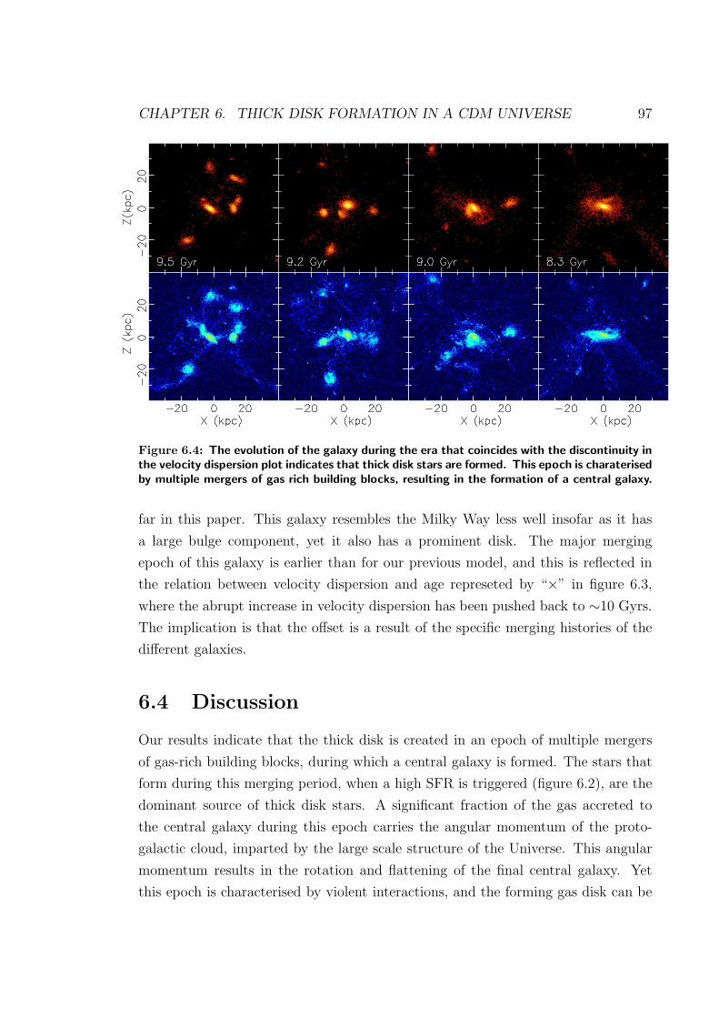
CHAPTER 6. THICK DISK FORMATION IN A CDM UNIVERSE 97
Figure 6.4: The evolution of the galaxy during the era that coincides with the discontinuity inthe velocity dispersion plot indicates that thick disk stars are formed. This epoch is charaterisedby multiple mergers of gas rich building blocks, resulting in the formation of a central galaxy.
far in this paper. This galaxy resembles the Milky Way less well insofar as it has
a large bulge component, yet it also has a prominent disk. The major merging
epoch of this galaxy is earlier than for our previous model, and this is reflected in
the relation between velocity dispersion and age represeted by “×” in figure 6.3,
where the abrupt increase in velocity dispersion has been pushed back to ∼10 Gyrs.
The implication is that the offset is a result of the specific merging histories of the
different galaxies.
6.4 Discussion
Our results indicate that the thick disk is created in an epoch of multiple mergers
of gas-rich building blocks, during which a central galaxy is formed. The stars that
form during this merging period, when a high SFR is triggered (figure 6.2), are the
dominant source of thick disk stars. A significant fraction of the gas accreted to
the central galaxy during this epoch carries the angular momentum of the proto-
galactic cloud, imparted by the large scale structure of the Universe. This angular
momentum results in the rotation and flattening of the final central galaxy. Yet
this epoch is characterised by violent interactions, and the forming gas disk can be

CHAPTER 6. THICK DISK FORMATION IN A CDM UNIVERSE 98
described as dynamically hot, resulting in the high velocity dispersion of the stars
forming in the disk. The result is the formation of a thick disk. Infalling gas after
this multiple merger epoch settles smoothly to a thin disk.
Several formation scenarios for the thick disk were presented by Gilmore et al.
(1989): 1) a slow, pressure-supported collapse that follows the formation of halo
Population II stars (Larson 1976); 2) violent dynamical heating of the early thin
disk by satellite accretion (Quinn et al. 1993) or violent relaxation of the Galactic
potential (Jones & Wyse 1983); 3) accretion of thick disk material directly (Statler
1988; Bekki & Chiba 2000; Abadi et al. 2003); 4) enhanced kinematic diffusion
of the thin disk stellar orbits (Norris 1987); and 5) a rapid dissipational collapse
triggered by high metallicity (Wyse & Gilmore 1988). To determine which of these
processes was the major driver of thick disk formation, observational evidence for
the metallicity, ages, and chemical abundances of thick disk stars may be compared
to the various predictions of each scenario.
Lack of a vertical metallicity gradient in the thick disk (Gilmore et al. 1995),
as well as a lack of large intermediate age thick disk population would seem to
rule out the slow collapse of scenario 1). The lack of overlapping age distributions
between thick and thin disk stars, as well as the discontinuity in their chemical
abundances, argues against the enhanced kinematic diffusion scenario 4). Further
evidence against such a scenario is the size of the discontinuity in velocity dispersion,
which appears to be too great to be explained by the known heating mechanisms,
i.e. local gravitational perturbations in the thin disk such as giant Molecular Clouds
(Spitzer & Schartzschild 1953) or transient spiral structure (Barbanis & Woltjer
1967; Carlberg & Sellwood 1985). Freeman (1991) suggested that these disk heat-
ing mechanisms saturate or become inefficient at σ ∼30 km/s. Lack of correlation
between the scale length of the thick and thin disk components of disk galaxies ob-
served by Dalcanton & Burnstein (2002, DB hereafter) also contradicts scenario 4)
for thick disk formation in other galaxies. If the thick disk were composed primarily
of material accreted slowly over time from many smaller satellites on suitable orbits,
as in scenario 3), then the metallicity of the stars would be too low to explain the
observed peak metallicity of the thick disk. The well known metallicity-mass rela-
tion of galaxies would require accretion of massive satellites (>1010 M), destroying
the thin disk, in order to obtain metallicities of [Fe/H]∼−0.6, unless the accreted
satellites are gas rich and the accretion process induces a significant self-enrichment
(Bekki & Chiba 2002). In addition, recent high resolution spectroscopic observa-
CHAPTER 6. THICK DISK FORMATION IN A CDM UNIVERSE 99
tions of individual stars in dwarf spheroidals (dSphs), find solar α-element to iron
abundance ratios (e.g. Shetrone et al. 2001, 2003) that differ significantly from
observed [α/Fe] and [Fe/H] in the thick disk. This indicates that the accretion of
systems similar to dSphs is not the dominant source of thick disk stars.
The heating of the disk early in its violent evolution, as in scenario 2), is well sup-
ported by Galactic observations (Quillen & Garret 2001; Wyse 2000; Gilmore et al.
2002; Freeman & Bland-Hawthorn 2002; FBL). This scenario is consistent with the
observed abrupt increase in velocity dispersions, the distinct chemical properties of
the two disk components, and the homogeneity of thick disk abundances. We con-
tend that our scenario of thick disk formation during the epoch of multiple mergers
of gas-rich building blocks is consistent with scenario 2), and hence with these ob-
servations of the Milky Ways thick disk. We note that the scenario 2) suggests two
possible heating mechanisms. In the first possible mechanism, a thin disk forms
and is heated by an accretion event. Our simulations more closely resemble the
mechanism of Jones & Wyse (1983), in which a thick disk forms during a violent
relaxation of the galactic potential, prior to the formation of the thin disk. Evidence
that the thick disk has had a more intense star formation history than the thin disk
(e.g. Bensby et al. 2003; MGTB) would seem to favour the mechanism we propose
over the “puffed up” thin disk, although neither mechanism proposed in scenario
2) is inconsistent with a rapid thick disk formation timescale (e.g. FBL). We note
also that the in situ formation of the thick disk in our scenario leads to efficient
self-enrichment. The increased cooling due to metals, as mentioned in scenario 5),
ensures a rapid star formation rate in the thick disk.
The formation of the thick disk in the manner we have outlined is a natural
consequence of the early, violent merging epoch of the CDM universe, indicating
that thick disks should be a common component of disk galaxies. Recent, deep
observations of a sample of 47 nearby edge-on galaxies by DB indicate that thick
disks are widespread around disk galaxies. A lack of correlation between thick and
thin disk scale lengths, as found by DB, is also explained by our formation scenario.
Confirmation of these findings would strengthen the case for our thick disk formation
scenario.

Chapter 7
Conclusions and Future Directions
The notion that stellar populations can be traced to their birthplace in the pro-
togalactic cloud through a study of their chemical and kinematic properties was
recently reviewed by Freeman & Bland-Hawthorn (2002), who nicknamed the pur-
suit “Galactic Archaeology”. However ambitious it may seem, Galactic Archaeology
is an instructive blueprint: it reminds us that processes and events at high redshift
are responsible for many current observations of the Milky Way. By interpreting
local observations within the context of the Cold Dark Matter paradigm, a connec-
tion is made with the distant Universe. Embracing an historical perspective, we
endeavour to unravel a detailed physical understanding of the sequence of events
which led to the formation of the Milky Way.
Prior to surveying present and future work, we present a brief summary of the
key results of this thesis:
• White dwarf stellar halo: As chemical signatures of white dwarf progenitor
stars, carbon and nitrogen abundances in the halo of a simulated galaxy were
compared with observations for the Galactic halo. This has enabled us to place
upper limits on the halo white dwarf population. Our results are inconsistent
with a white dwarf component in the halo >∼ 5 % (by mass), however mass
fractions of ∼1-2 % cannot be ruled out.
• Milky Way substructure: The dynamical signatures of the formation of the
stellar halo were examined. A group of simulated high-eccentricity stars were
traced to disrupted satellites that had been accreted by the host galaxy. The
phase space distribution of the accreted stars were compared with observed
100
CHAPTER 7. CONCLUSIONS AND FUTURE DIRECTIONS 101
high-eccentricity stars in the solar neighbourhood, providing evidence for a
“stellar stream” in our own Galaxy.
• Constraints set by the stellar halo: The observed low metallicity and low
mass of the Galactic stellar halo are typically invoked to constrain disk galaxy
formation models. We demonstrate the importance of strong feedback - the
mechanism that regulates star formation in Galactic building blocks - to mod-
els that successfully conform to observational constraints.
• Thick disk formation: An abrupt increase in the velocity dispersion versus
stellar age relation provides evidence that a thick disk forms in our simulated
disk galaxy. The thick disk in our simulation forms in a chaotic merging period
at early epochs of galaxy formation. This formation scenario for the thick disk
component of the Milky Way is shown to be consistent with observations.
Some of the following investigations have arisen directly from the issues raised
by this thesis.
• Heating of disk stars: Heating of the thin disk stars by local gravitational
disturbance or transient spiral structure was ruled out as the origin of the
thick disk in chapter 6. However, recent results of Nordstrom et al. (2004)
indicate that the kinematic diffusion of the thin disk has been enhanced over
the past 8-10 Gyrs, presumably by mechanisms similar to those mentioned
above. Preliminary analysis suggests that stars in our simulated thin disk do
exhibit signs of heating. We intend to develop an explanatory framework for
the observations by determining the influential parameters for the heating in
our simulations.
• Statistical thick disk study: By examining a statistically significant number
of simulated disk galaxies similar to the one examined in chapter 6, with
varying masses, angular momentum and merging histories, we hope to predict
the expected frequency of thick disks and to characterise thick disk properties
such as age, metallicity and colour of the stellar populations.
• Substructure: Martin et al. (2004) have published evidence that a satellite
has recently been accreted by the Milky Way, resulting in a population of stars
with thick disk characteristics. Simulations by Abadi et al. (2004) suggest that

CHAPTER 7. CONCLUSIONS AND FUTURE DIRECTIONS 102
thick disk formation processes are dominated by accretion events. However,
the scenario presented in chapter 6, in which the thick disk forms in an epoch of
merging and high star formation early in the Galaxy’s evolution, implies that
only a minor proportion of thick disk stars are directly accreted. These studies
are in addition to the now established role that accretion plays in building up
the stellar halo (e.g. Ibata et al. 1994, Helmi et al. 2000, chapter 4 of this
thesis). By combining new observations, such as those from the Sloan Digital
Sky Survey, the Radial Velocity Experiment (RAVE) and GAIA (see below),
we hope that the full extent to which accretion has contributed to both the
stellar halo and thick disk will be revealed.
• σV versus RGAL: Toomre (1964) demonstrated that the stability of a uniform
cold disk requires the parameter, Q, to be greater than unity, where
Q =σRκ
3.36GΣ, (7.1)
σR is the radial component of velocity dispersion, κ is the local epicyclic fre-
quency, Σ is the surface density, and G is the gravitational constant. Lewis
& Freeman (1989) observe a relation between radial velocity dispersion and
radius of the old Galactic disk, as would be implied from the Toomre parame-
ter for a stable disk. Preliminary analysis of our simulations reveals a similar,
if slightly weaker, negative trend of σR versus RGAL to those observed. We
intend to investigate the significance of this divergence from the observational
data.
• Self-consistent elliptical and disk simulations: Models for simulating disk and
elliptical galaxy formation have often required use of different values of various
parameters, such the spin parameter. A further test of the feedback algorithm
introduced in chapter 5 is to apply it to initial conditions that result in realistic
elliptical galaxies as well as disk galaxies. Our preliminary studies of this are
promising. We have run the Adiabatic Feedback Model (AFM, chapter 4) with
the initial conditions of 2 × 10¹¹ and 8 × 10¹¹ solar masses from Kawata &
Gibson (2003a). The resultant galaxies are morphologically elliptical. We
have not yet completed a detailed analysis of these simulations, but we do find
that star formation is ongoing at redshift zero. A further line of inquiry in this
project will be to examine whether applying the AFM to SNe Ia affects the

CHAPTER 7. CONCLUSIONS AND FUTURE DIRECTIONS 103
ongoing star formation in ellipticals, and determining the effect of feedback
from SNe Ia on disk galaxies.
• Cosmological simulations with GCD+: In this thesis, a semi-cosmological ver-
sion of GCD+ was employed. As was prefaced in chapter 1, advantages exist
in using a full cosmological code. Full cosmological simulations permit galaxy
simulations with realistic halo masses, merging histories and tidal forces, i.e.
the properties that ultimately provide angular momentum and determine the
collapse redshift. A cosmological version of GCD+ employs the multi- resolution
technique to simulate galaxy formation (Kawata & Gibson 2003b). A galaxy
that resembles the Milky Way has been identified within GCD+ cosmological
simulations (Gibson et al. 2003). We plan to employ the AFM to make mock
observations of the simulated galaxy, and then to compare the “observed” val-
ues of angular momentum with the values derived directly from the simulated
end products. A study such as this is not possible with a semi-cosmological
model since a solid body spin parameter is included in the initial conditions.
• Comparing galaxy formation models: As noted in chapter 1, several different
methods are used to model the formation of the Milky Way. Semi-analytic
chemical galaxy evolution models of the Milky Way are able to reproduce
the solar neighbourhood metallicity distribution function (MDF), e.g. Fenner
& Gibson (2003), as well as broad chemical trends. Our simulations, using
both the semi- and full- cosmological versions of GCD+, have also reproduced
the local MDF and similar chemical trends. In all codes, these results are
influenced by outflows and inflows of gas of varying chemical composition. It
would be interesting to compare these models, to evaluate dynamical effects
on the chemical evolution, and assess the different gas mixing assumptions of
the two types of codes.
• Disk-dark matter alignment: Knebe et al. (2003) recently showed that the
orbits of simulated galaxy cluster sub-halos are biased to lie along the major
axis of the cluster, due to infall along filaments. They postulated that this
bias may explain the Holmberg effect, if galaxy disks are perpendicular to the
major axis of their dark matter halos. Using results from cosmological GCD+
disk galaxy simulations, we hope to establish how disks align with the tri-axial
halos in which they reside.
CHAPTER 7. CONCLUSIONS AND FUTURE DIRECTIONS 104
Galactic astronomy will remain an exciting field for theorists and observers over
the next decade and beyond. Planned surveys will provide an extraordinary abun-
dance of information about the Milky Way’s components. Moore’s law coupled with
sophisticated galaxy formation algorithms promise increasingly detailed modeling
at higher and higher resolution. We embarked on the “journey” of this thesis by
describing the sequence of discoveries that established our current understanding of
our Galaxy and its constituents. Arriving at our present (albeit temporary) desti-
nation, it is perhaps fitting that we should preview the next historic phase of Milky
Way exploration.
New Views of the Milky Way
For studies of the Milky Way, an exciting new observational era approaches. To
understand the evolution of the Galaxy in a quantitative sense, it will be imperative
to know the full multivariate distribution of stars over parameters such as age,
metallicity, the three components of velocity, and the components of position. In
particular, two new surveys, RAVE and GAIA promise to transform our knowledge
of the stars that populate the Milky Way.
RAVE will conduct an all-sky survey to measure radial velocities, metallicities,
and abundance ratios for 50 million stars. Phase I of RAVE is under way, using
the UK Schmidt Telescope to survey 100,000 stars over 10,000 square degrees to
I=12. Phase II will cover the sky to I=15, include 50 million stars, and run from
2006 to 2010. RAVE will provide a truly representative inventory of stellar radial
velocities for all major components of the Galaxy; 26 million thin disk main sequence
stars, 9 million thick disk stars, 2 million bulge stars, 1 million halo stars, and
12 million giant stars. The ability to combine the radial velocities with proper
motions and parallaxes from other sources (USNO, Tycho-2, Hipparcos, GAIA)
should accomplish an extraordinary advance in our understanding of our Galaxy.
The GAIA satellite is due for launch in 2010. The goal is to make the largest,
most precise map of our Galaxy by surveying more than one billion stars, about one
per cent of our Galaxy’s population. GAIA will detect the motion of each star in
its orbit around the Galactic Centre. GAIA will compile a complete sample of G
sub-giants, which provide the most accurate ages for individual older stars, along
with accurate kinematics and distances. The GAIA sample comprises a very signif-
icant radial zone in the Galactic disk: about 2 to 4 scale lengths from the Centre.
CHAPTER 7. CONCLUSIONS AND FUTURE DIRECTIONS 105
Ground-based metallicity data will complement chemical abundance estimates.
To interpret such unprecedented data sets, and disentangle the formation history
of the Milky Way, theoretical models which can directly compare with observation
are required. This will ensure that chemo-dynamical models for Milky Way forma-
tion continue to play an important role in Galactic Archaeology.

Bibliography
Aarseth S. 1963, MNRAS, 126, 223
Aaronson M. 1987 in Nearly normal galaxies: From the Planck time to the present;
Proceedings of the Eighth Santa Cruz Summer Workshop in Astronomy and As-
trophysics. New York, Springer-Verlag, 57-66.
Abadi M. G., Navarro J. F. & Steinmetz M. 2003, ApJ, 597, 21
Abadi M. G., Navarro J. F., Steinmetz M. & Eke V. R. 2003, ApJ, 591 499
Abia C., Dominguez I., Straniero O., Limongi M., Chieffi A., Isern J. 2001, ApJ,
557, 126
Abel T., Bryan G. & Norman M. 1999, in Space, meeting held in Paris, France,
September 28th - October 1st, eds.F. Combes, G. Pineau des Forets. Cambridge
University Press, Astrophysic Series
Abel T., Bryan G., Norman M. 2002, Science, 295, 5552, 93
Adams F. C. & Laughlin G. 1996, ApJ, 468, 586
Alcock C. et al., 2000 ApJ, 542, 281
Balsara D. 1995 AAS, 187 5204
Barnes J.E. & Hut P. 1986, Nature, 324, 446
Beers T.C. et al. 2002, AJ, 124, 931
Beers T. C. & Sommer-Larsen J. 1995, ApJS, 96, 175
Bekki K. & Chiba M. 2001, ApJ, 558, 666
106

BIBLIOGRAPHY 107
Bekki K. & Chiba M. 2000, ApJ, 534, 89
Bekki K. & Shioya Y. 1998, ApJ, 497, 108
Bekki K. & Shioya Y. 1999, ApJ, 531, 108
Bensby T., Feltzing S., & Lundstrom I. 2003, A&A, 410, 527
Berczik P. 1999, A&A, 348, 371
de Bernardis P. et al. 2000, Nature, 404, 955
Bertschinger E., 2001 ApJS 137 1
Bromm V., Ferrara A., Coppi P. S. & Larson, R. B. 2001, AAS, 198, 603
Brook C. B, Kawata D. & Gibson Brad K. 2003, ApJ, 585 125
Brook C. B, Kawata D., Gibson Brad K., & Flynn C. 2004, MNRAS, 349, 52
Bruzual G. & Charlot S. 2003 MNRAS 344, 1000
Burkert, A. 2001, in Cosmic Evolution, Institut d’Astrophysique de Paris, eds.
Vangioni-Flam E., Ferlet R., & Lemoine M. New Jersey: World Scientific, p.245
Burton W. B. & Lockman F. J. 1999, A&A, 349, 7
Carlberg R. G. 1984a ApJ, 286, 403
Carlberg R. G. 1984b ApJ, 286, 416
Carlberg R. G., Lake G. & Norman C. A. 1986 ApJ, 300, L1
Carney B. W., Latham D. W. & Laird J. B. 1990 AJ, 99, 201
Carney B. W., Latham D. W., Laird J. B. & Aguilar L. A. 1994 AJ, 107, 2240
Chaboyer B., Demarque P., Kernan P. J., & Krauss L. M. 1998, ApJ, 494, 96
Chabrier G., Segretain L. & Mera D. 1996, ApJ, 486, L21
Chen Y. Q., Nissen P. E., Zhoa G., Zhang H. W. & Benoni T. 2000, A&AS, 141,
491
Chiba M. & Beers T. C., 2000, AJ, 119, 2843

BIBLIOGRAPHY 108
Clemens D. P. 1985, ApJ, 295, 422
Cole S., Aragon-Salamanca A., Frenk C. S., Navarro J. F. & Zepf S. E. 1994, MNRAS
271, 781
Cole S., Lacey C. G., Baugh C. M. & Frenk C. S., 2000 MNRAS, 319, 168
Creze M., Chereul E., Bienayme O. & Pichon C. 1998 A&A 329 920
Christlieb N. et al. 2002 Nature, 419, 904
Dalcanton J. J. & Bernstein R. A. 2002, AJ, 124, 1328
Dalcanton J. J., Spergel D. N. & Summers F. J. 1997 ApJ, 482, 659
Davies R. L., Frogel J. A. & Terndrup D. M., 1991 AJ 102 1729
Davidge T. J. & Courteau S. 2002 AJ 123 1438
Dominguez I., Straniero O., Limongi M. & Chieffi A., 1999, ApJ, 524, 226
Dinescu, D. I 2002 in Omega Centauri: A Unique Window into Astrophysics, eds.
F. van Leeuwen, G. Piotto & J. Hughes (San Francisco: ASP)
Durrell P. R., Harris W. E. & Pritchet C. J. 1994, AJ, 108, 2114
Edvardsson B., Anderson J., Gustafsson B., Lambert D. L., Nissen P. E. & Tomkin
J. 1993, A&A 275, 101
Eggen O. J., Lynden-Bell D. & Sandage A. R. 1962, ApJ, 136, 748
Eke V. R., Cole S. & Frenk C. S. 1996, MNRAS, 282, 263
Fall S. M. & Efstathiou G. 1980 MNRAS, 193, 189
Feltzing S., Bensby T. & Lundstrom I. 2003, A&A, 397, 1
Fenner Y. & Gibson B. K. 2003, PASA, 20, 189
Fich M., Blitz L. & Stark A. A. 1989, ApJ, 342, 272
Fields B. D., Freese K. & Graff D. S. 2000, ApJ, 534, 265
Flynn C., Gould A. & Bahcall J. 1996, ApJ, 466, L55
BIBLIOGRAPHY 109
Flynn C., Holopainen J. & Holmberg J. 2003, MNRAS, 339, 817
Flynn C., Sommer-Larsen J., Fuchs B., Graff D.S. & Salim S. 2001, MNRAS, 322,
553
Freeman K. C, 1987 ARA&A, 25, 603
Freeman K. C. 1991, in Dynamics of Disk Galaxies, eds. B. Sundelius, (Goteborgs
University and Chalmer University of Technology, Goteborg Sweden), 15
Freeman K. C & Bland-Hawthorn J. 2002 ARAA, 40, 487
Frei Z., Guhathakurta P., Gunn J. E. & Tyson J. A. 1996 AJ,111,174
Frogel J.A., 1990, in ESO/CTIO Workshop on Bulges of Galaxies ESO, Garching,
A92-18101 05-90, 177
Fuhrmann K., 1998, A&A, 338, 161
Fry A. M., Morrison H. L., Harding P. & Boroson T. A. 1999 AJ 118 1209
Gerritsen J. P. E. 1997, Ph.D. thesis, Kapetyn Ast. Inst.
Gibson B.K. et al. 2000 ApJ 529 723
Gibson B.K. & Flynn C. 2001 Science, 292, 2211
Gibson B.K. & Mould J.R. 1997, ApJ, 482, 98 (GM97)
Gilmore, G., 2001, in Starbursts: Near and Far, eds. Tacconi, L.J., Lutz, D.,
Springer-Verlag, Heidelberg, 34
Gilmore, G. 2003, in Galaxy Evolution: Theory and Observations eds. V. Avila-
Reese, C. Firmani, C. Frenk & C. Allen Rev Mex AA, CS, vol. 17, 149
Gilmore G., & Reid N. 1983, MNRAS, 202, 1025
Gilmore G., Wyse R. F. G. & Kuijken K. 1989, ARA&A, 27, 555
Gilmore G., Wyse R. F. G. & Jones J. B. 1995, AJ, 109, 3
Gilmore G., & Wyse R. F. G. 1985, AJ, 90, 2015
Gingold R. A., Monaghan J. J. 1977, MNRAS, 181, 375
BIBLIOGRAPHY 110
Girardi L., Bressan A., Bertelli G. & Chiosi C. 2000, A&AS, 141, 371
Goldman B. et al. 2002, A&A, 389, 69
Gould A., Flynn C. & Bahcall J. 1998, ApJ, 503, 798
Gratton R. G., Carretta E., Matteucci F. & Sneden C. 2000, A&A, 358, 671
Gratton R. G., Bragaglia A., Carretta E., Clementini G., Desidera S., Grundahl F.,
Lucatello S. 2003 A&A, 408, 529
Gyuk G. & Gates E. 1999, MNRAS, 304, 281
Hansen B. M. S. 1998 Nature, 394, 798
Hansen B. M. S. 2001, ApJ, 558, L39
Harris H. C. et al. 2001, ApJ, 549, L109
Helmi A. 2004 MNRAS in press
Helmi A., White S. D. M., de Zeeuw P. T. & Zhao H. 1999, Nature 402 53
Helmi A. & White S. D. M. 1999, MNRAS, 307, 495
Helmi A. & de Zeeuw H. S. 2000, MNRAS, 319, 657
Hernquist L. & Katz N. 1989, ApJS, 70, 419
Hodgkin S. T. et al., Nature, 2000, 403, 57
Honma M. & Sofue Y. 1997, PASJ, 49, 539
Hodge P. W. 1983 PASP, 95, 721
Hultman J. & Pharasyn A. 1999, A&A, 347, 769
Huchra J. & Brodie J. 1987, AJ, 93, 779
Ibata R. & Gilmore G. 1995, MNRAS, 275, 605
Ibata R., Gilmore G. & Irwin M. J. 1994, Nature, 370, 194
Ibata R.A., Irwin M., Bienayme, O., Scholz R. & Guibert J. 2000, ApJ, 532, L41

BIBLIOGRAPHY 111
Ibata R. A., Irwin M. J., Lewis G. F., Ferguson A. M. N. & Tanvir N. 2003 MNRAS
340 21
Ibata R. A., Richer H. B., Gilliland R. L. & Scott D. 1999, ApJ, 524, 95
Ibata R., Lewis G. F., Irwin M., Totten E. & Quinn T. 2001 ApJ 551 294
Iwamoto K., Brachwitz F., Nomoto K., Kishimoto N., Umeda H., Hix W. R &
Thielemann F-K. 1999, ApJS, 125, 439
Kaellander D. & Hultman J. 1998, A&A, 333, 399
Katz N., 1992, ApJ, 391, 502
Katz N. & Gunn J.E. 1991, ApJ, 377, 365
Katz N. 1992 ApJ, 391, 502
Katz N., Weinberg D. H., Hernquist L. 1996, ApJS, 105, 19
Kauffmann G. 1996 MNRAS, 294, 705
Kauffmann G., White S. D. M. & Guiderdoni B. 1993 MNRAS, 264, 201
Kay S.T., Pearce F.R., Jenkins A. et al. 2000, MNRAS, 316, 374
Kay S. T., Pearce F. R., Frenk C. S. & Jenkins A. 2002, MNRAS, 330, 113
Kawata D. 1999, PASJ, 51, 931
Kawata D. 2001, ApJ, 548, 703
Kawata D. & Gibson B. K. 2003a, MNRAS, 340, 908
Kawata D. & Gibson B. K. 2003b, MNRAS, 346, 135
Klypin A., Kratsov A. V., Valenzuela O. & Prada F. 1999, ApJ, 522, 8
Knebe A., Gill S. P. D., Gibson B. K., Lewis G. F., Ibata R. A. & Dopita M. A.
2004, ApJ, 603, 7
Koda J., Sofue Y. & Wada K. 2000, ApJ, 531, 17
Kobayashi C. 2002, Ap&SS, 281, 301
BIBLIOGRAPHY 112
Kobayashi C., Tsujimoto T. & Nomoto K. 2000 ApJ, 539 26
Kobayashi C. 2004 MNRAS 347 740
Kato M. 1998, ApJ, 503, 155
Kochanek C. S. 1996 ApJ, 457 228
Kotenova E., Flynn C., Chiappini C. & Matteucci F. 2002, MNRAS, 336, 879
Koribalski B., Johnston S. & Otrupcek R. 1994, MNRAS, 270, 43
Kroupa P. 2001, MNRAS, 322, 231
Kuijken K. 1996, in ASP Conf. Ser. 91, Barred Galaxies, eds. R. Buta, D. A. Crocker
& B. G. Elmegreen (San Francisco: ASP), 504
Larson R. B. 1969 MNRAS, 145, 405
Larson R. B. 1974a MNRAS, 166, 585
Larson R. B. 1974b MNRAS, 169, 229
Larson R. B. 1969 MNRAS, 173, 671
Lasserre T. et al. 2000, A&A, 355, 39
Lee Y-W., Joo J.-M., Sohn Y.-J., Rey S.-C., Lee H.-C. & Walker A. R. 1999, Nature,
402, 55
Lewis J. R. & Freeman K. C. 1989 Astron. J, 97, 139
Leggett S. K., Ruiz M. T. & Bergeron P. 1998, ApJ, 497, 294
Lin C. C. & Shu F. H. 1964, ApJ, 140, 646
Limongi M. & Chieffi A. 2003 in From Twilight to Highlight: The Physics of Su-
pernovae. Proceedings of the ESO/MPA/MPE Workshop, Garching, Germany, p.
367.
Lucy L. 1977, AJ, 82, 1013
Loewenstein M. & Mushotzky R. F. 2001 AAS, 199 2505

BIBLIOGRAPHY 113
Majewski S. R., Munn J. E. & Hawley S. L. 1996, ApJ, 459, 73
Makino J. 1991 PASJ, 43 859
Marigo P., Bressan A. & Chiosi C., 1996, A&A, 313, 545
Marigo P., Girardi L., Chiosi C. & Wood P. R. 2001, A&A, 371, 152
Mashonkina L. & Gehren T. 2001, A&A, 376, 232
Mashonkina L., Gehren T., Travaglio C. & Borkova T. 2003 A&A, 397, 275
Mateo M. L. 1998 ARA&A, 36, 435
Matteucci F. & Francois P. 1989, MNRAS, 239, 885
Martin N. F., Ibata R. A., Bellazzini M., Irwin M. J., Lewis G. F. & Dehnen W.
2004, MNRAS, 348, 12
McGaugh S. S. & De Block W. J. G. 1998, ApJ, 499, 41
Mendez R. A. 2002, A&A, 395, 779
Mendez R. A. & Minniti D. 2000 ApJ, 529, 911
Mera D., Chabrier G. & Schaeffer R., 1998, A&A. 330, 953
Mighell K. J. & Rich R. M. 1995 AAS, 186, 3906
Mo H. J., Mao S. & White S. D. M. 1998 MNRAS, 295 319
Morrison H. L. 1993, Astron. J., 106, 578
Moore B., Ghigna S., Governato F., Lake G., Quinn T., Stadel J. & Tozzi P. 1999,
ApJ, 524, 19
Mori M., Yoshii Y. & Nomoto K. 1999, ApJ, 511, 585
Mulchaey J. S., Davis D. S., Mushotzky R. F. & Burstein D. 1993 ApJ, 404, 9
Mushotzky R. F. & Loewenstein M., Awaki H., Makishima K., Matsushita K. &
Matsumoto H. 1994, ApJ, 436, L79
Nakamura F. & Umemura M. 2001, ApJ, 548, 19

BIBLIOGRAPHY 114
Nakasato N. & Nomoto K. 2003, ApJ 588 842
Navarro J. F., Frenk C. S. & White S. D. M. 1995 MNRAS, 275, 56
Navarro J. F., Frenk C. S. & White S. D. M. 1997, ApJ, 490, 493
Navarro J. F. & Steinmetz M. 1997, ApJ, 478, 13
Navarro J. F. & Steinmetz M. 2000, ApJ, 538, 477
Navarro J. F & White S. D. M. 1993, MNRAS, 265, 271
Nelson C. A., Cook K. H., Axelrod T. S., Mould J. R. & Alcock C. 2002, ApJ, 573,
644
Nissen P. E. & Schuster W. J. 1997, A&A, 326, 751
Nordstrom B. et al. 2004, A&A in press
Ojha D. K. 2001, MNRAS, 322, 426
Oppenheimer B. R. et al. 2001, Science, 292, 698
Ostriker J. P. & Peebles P. J. E. 1973 ApJ, 186, 467
Phelps S., Meisenheimer K., Fuchs B., Wolf C. & Jahreiss H. 1999, in Galaxy Evolu-
tion: Connecting the Distant Universe with Local Fossil Record, Obs de Meudon,
1998.
Padmanabham T. 1993 Structure Formation in the Universe, Cambridge Univ.
Press, Cambridge
Pagel B. E. J. & Tautaisiene G. 1995, MNRAS, 276, 505
Peebles P. J. E. 1969, ApJ, 155, 393
Peebles P. J. E. 1971, A&A, 11, 377
Prochaska J. X., Naumov S. O., Carney B. W., McWilliam A. & Wolfe A. M. 2000,
ApJ, 120, 2513
Quillen A. C. & Garnett D. 2001. in Galaxy Disks and Disk Galaxies, ASP Conf.
Ser., eds. G. Jose, S. J. Funes, E. M. Corsini, 230:87-88. San Francisco: Publ.
Astron. Soc. Pac.
BIBLIOGRAPHY 115
Raiteri C. M., Villata M. & Navarro J. F. 1996, A& A, 315, 105
Reddy B. E., Tomkin J., Lambert D. L. & Allende Prieto C. 2003, MNRAS, 340,
304
Reid N., Sahu K. C. & Hawley S. 2001, ApJ, 559, 942
Renzini A. & Voli M. 1981, A&A, 94, 175
Reyle C., Robin A. C. & Creze M. 2001, A&A, 378, L53
Rich R. M. 2001 in Astrophysical Ages and Timescales, eds. T. van Hippel, N.
Mansuset & C. Simpson, ASP Conf. Ser. 245, 216
Richer H. B., 2001, in The Dark Universe: Matter, Energy and Gravity, ed. M.
Livio, Cambridge Univ. Press, Cambridge
Ryan S. G. & Norris J. E. 1991, AJ, 101, 1865
Salpeter E. E. 1955 ApJ, 121, 161
Sauman D. & Jacobson S. B. 1999, ApJ, 511, L107
Scalo J. M. 1986, Fund. Cosm. Phys., 11, 1
Schroder K. P. & Pagel B. E. J. 2003, MNRAS, 343, 1231
Schmidt B. P. et al. 1998 ApJ 507, 46
Searle L. & Zinn R. 1978, ApJ, 255, 357
Schaller G., Schaerer D. & Meynet G. 1992, A&AS, 96, 269
Somerville R. S. 2002 ApJ, 572, 23
Somerville R. S. & Primack J. R. 1999 MNRAS, 310, 1087
Spergel et al. 2003 ApJS, 148, 175
Springel V. & Hernquist L. 2003, MNRAS, 339, 289
Steinmetz M. 1996, MNRAS 278, 1005
Steinmetz M. & Muller E. 1994, A&A, 281, L97

BIBLIOGRAPHY 116
Steinmetz M. & Muller E. 1995, MNRAS, 276, 549
Steinmetz M. & Navarro J. F. 1999, ApJ, 513, 555
Steinmetz M. & Navarro J. F. 2002, NewA, 7, 155
Strauss M. A. & Willick J. A. 1995, Phys. Rep., 261, 271
Stompor R. et al. 2001, ApJL, 561, 7
Sutherland R. S. & Dopita M. A. 1993, ApJS, 88, 253
Tautaisiene G., Edvardsson B., Tuominen I. & Ilyin I. 2001, A&A, 380, 578
Talbot R. J. & Arnett D. W. 1971, ApJ, 170, 409
Talbot R. J. & Arnett D. W. 1975, ApJ, 197, 551
Thacker R. J. & Couchman H. M. P. 2000, ApJ, 545, 728
Theis C., Burkert A. & Hensler G. 1992, A&A, 265, 465
Timmes F. X., Woosley S. E. & Weaver T. A. 1995, ApJS, 98,617
Tinsley B. M. 1980, Fund. Cosm. Phys., 5, 287
Torres S., Garcia-Berro E., Burkert A. & Isern J. 2001, MNRAS 328, 492
Tripicco M. J. & Bell R. A. 1995 AJ 110 3035
Tyson J. A., Wenk R. A. & Valdes F. 1990 ApJL, 349, L1
van den Bergh, S. 1999 A&AR 9, 273
van den Hoek L. B. & Groenewegen M. A. T. 1997, A&AS, 123, 305
von Hoerner S., 1963 Z. Astrophys. 57, 47.
van Loon J. Th., Gilmore G. F., Omont A., Blommaert J A. D. L., Glass I. S.,
Messineo M., Schuller F., Schultheis M., Yamamura I. & Zhao H. S. 2003 MNRAS
338 857
Vazdekis A., Casuro E., Peletier R. F. & Beckman J. E. 1996, ApJS, 106, 307
BIBLIOGRAPHY 117
Walker T. P., Steigman G., Kang H., Schramm D. M. & Olive K. A. 1991 ApJ, 376,
51
White S. D. M., Navarro J. F., Evrard A. E. & Frenk C. S. 1993, Nature, 366, 429
White S. D. M. & Rees M. J. 1978 MNRAS 183 341
White S.D.M. & Springel V., 2000, in The First Stars,eds. A. Weiss, T.G. Abel, V.
Hill, Spinger-Verlag, Heidelberg, 327
White S. D. M. & Frenk C. S. 1991, ApJ, 379, 52
Wilkinson M. I. & Evans, N. W. 1999, MNRAS, 310, 645
Woosley S. E., Weaver, T. A. 1995, ApJS, 101, 181
Worthey G. 1994, ApJS, 94, 687
Wu K., Lahav O. & Rees M. 1999, Nature, 397, 225
Wyse R. F. G. 1999, Baltic Astronomy, 8, 593
Wyse R. F. G. & Gilmore G. 1995, AJ 110, 2771
Yoshii Y. & Saio H. 1986, ApJ, 301, 587
Zibetti S., White S. D. M. & Brinkmann J. 2004, MNRAS, 347, 556
Zaritsky D. in The Third Stromlo Symposium: The Galactic Halo ASP Conference
Series, eds. B.K. Gibson, T.S. Axelrod, M.E. Putman, Vol 165, 1999, p. 34
Zaroubi S., Zehavi I., Dekel A., Hoffman Y. & Kolatt T. 1997, ApJ, 486, 21
Zinn R. 1985, ApJ, 293, 424
Publications
List of Publications
Refereed Journals
[6] C. B. Brook, D. Kawata, B. K. Gibson, K. C. Freeman:
The Emergence of the Thick Disk in a CDM Universe
Astrophys. J. submitted
[5] H.-C. Lee, B. K. Gibson, Y. Fenner, C. B. Brook, D. Kawata, A. Renda,
J. Holopainen, C. Flynn:
Photometric Properties of White Dwarf Dominated Halos
accepted for publication in PASA
[4] C. B. Brook, D. Kawata, B. K. Gibson, C. Flynn:
Stellar Halo Constraints on Simulated Late-type Galaxies
Mon. Not. R. Astron. Soc. 349, 52 (2004)
[3] C. B. Brook, D. Kawata, B. K. Gibson:
Simulating a White Dwarf-dominated Galactic Halo
Mon. Not. R. Astron. Soc. 343, 913 (2003)
[2] C. B. Brook, D. Kawata, B. K. Gibson, C. Flynn:
Galactic Halo Stars in Phase Space: A Hint of Satellite Accretion?
Astrophys. J. Letter 585, 125 (2003)
[1] C. B. Brook, D. Kawata, B. K. Gibson, C. Flynn:
On the origin of high eccentricity halo stars
Astrophys. & Sp. Sci. 284, 845 (2003)

Proceedings
[3] C. B. Brook, D. Kawata, B. K. Gibson:
Phase Space Plots of Streams in the Halo, and their Chemical Tags
in Satellites and Tidal Streams, ING-IAC Joint Conference
eds. D. Martnez-Delgado & F. Prada, in press
[2] C. B. Brook, D. Kawata, B. K. Gibson, C. Flynn:
Simulating a White Dwarf Dominated Halo
in Astrophysical Supercomputing using Particle Simulations,
eds. J. Makino & P. Hut, (ASP, San Franciso), 381-382
[1] B. K. Gibson and C. B. Brook
Type Ia Supernovae and the Value of the Hubble Constant
in New Cosmological Data and the Values of the Fundamental Parameters
(IAU Symposium #201)
eds. A. Lasenby & A. Wilkinson, ASP Conference Series
Oral Presentations
[3] Phase Space Plots of Streams in the Halo, and their Chemical Tags
at Satellites and Tidal Streams, ING-IAC Joint Conference
La Palma, Canary Islands, Spain, May 26-30, 2003
[2] High eccentricity halo stars in phase spase
at The Evolution of Galaxies III, Kiel, Germany, July 2002
[1] The origin of high eccentricity halo stars
at the Astronomical Society of Australia Annual Science Meeting,
Mollymook, Australia, June 2002