Chemistry 155 Introduction to Instrumental … Lecture 2009...Chem 155 Unit 1 Page 1 of 313 Page 1 of 313 Chemistry 155 Introduction to Instrumental Analytical Chemistry Unit 1 Spring

Chem 155 Unit 1 Page 1 of 313

Page 1 of 313

Chemistry 155 Introduction to Instrumental

Analytical Chemistry Unit 1 Spring 2009 San Jose State University Roger Terrill


Page 2 of 313

1 Overview and Review ........................................................................................ 7 2 Propagation of Error ......................................................................................... 56 3 Introduction to Spectrometric Methods ............................................................ 65 4 Photometric Methods and Spectroscopic Instrumentation ............................... 86 5 Radiation Transducers (Light Detectors): ...................................................... 100 6 Monochromators for Atomic Spectroscopy: ................................................... 114 7 Photometric Issues in Atomic Spectroscopy .................................................. 134 8 Practical aspects of atomic spectroscopy: ..................................................... 148 9 Atomic Emission Spectroscopy ...................................................................... 159 10 Ultraviolet-Visible and Near Infrared Absorption .......................................... 174 11 UV-Visible Spectroscopy of Molecules ........................................................ 192 12 Intro to Fourier Transform Infrared Spectroscopy ........................................ 208 13 Infrared Spectrometry: ................................................................................. 231 14 Infrared Spectrometry - Applications ............................................................ 244 15 Raman Spectroscopy: .................................................................................. 256 16 Mass Spectrometry (MS) overview: ............................................................. 276 17 Chromatography .......................................................................................... 291


Page 3 of 313

1 Overview and Review ........................................................................................ 7

1.1 Tools of Instrumental Analytical Chem. ................................................ 8 1.2 Instrumental vs. Classical Methods. ................................................... 12 1.3 Vocabulary: Basic Instrumental .......................................................... 13 1.4 Vocabulary: Basic Statistics Review .................................................. 14 1.5 Statistics Review ................................................................................ 15 1.6 Calibration Curves and Sensitivity ...................................................... 23 1.7 Vocabulary: Properties of Measurements .......................................... 24 1.8 Detection Limit ................................................................................... 25 1.9 Linear Regression .............................................................................. 31 1.10 Experimental Design: ....................................................................... 35 1.11 Validation – Assurance of Accuracy: ................................................ 43 1.12 Spike Recovery Validates Sample Prep. .......................................... 45 1.13 Reagent Blanks for High Accuracy: .................................................. 46 1.14 Standard additions fix matrix effects:................................................ 47 1.15 Internal Standards ............................................................................ 52

2 Propagation of Error ......................................................................................... 56 3 Introduction to Spectrometric Methods ............................................................ 65

3.1 Electromagnetic Radiation: ................................................................ 66 3.2 Energy Nomogram ............................................................................. 67 3.3 Diffraction ........................................................................................... 68 3.4 Properties of Electromagnetic Radiation: ........................................... 71

4 Photometric Methods and Spectroscopic Instrumentation ............................... 86 4.1 General Photometric Designs for the Quantitation of Chemical Species ................................................................................................................. 87 4.2 Block Diagrams .................................................................................. 88 4.3 Optical Materials ................................................................................ 89 4.4 Optical Sources .................................................................................. 90 4.5 Continuum Sources of Light: .............................................................. 91 4.6 Line Sources of Light: ........................................................................ 92 4.7 Laser Sources of Light: ...................................................................... 93

5 Radiation Transducers (Light Detectors): ...................................................... 100 5.1 Desired Properties of a Detector: ..................................................... 100 5.2 Photoelectric effect photometers ...................................................... 101 5.3 Limitations to photoelectric detectors: .............................................. 103 5.4 Operation of the PMT detector: ........................................................ 104 5.5 PMT Gain Equation: ......................................................................... 105

6 Monochromators for Atomic Spectroscopy: ................................................... 114 6.1 Adjustable Wavelength Selectors ..................................................... 115 6.2 Monochromator Designs: ................................................................. 116 6.3 The Grating Equation: ...................................................................... 117 6.4 Dispersion ........................................................................................ 120 6.5 Angular dispersion: .......................................................................... 121 6.6 Effective bandwidth .......................................................................... 123 6.7 Bandwith and Atomic Spectroscopy ................................................. 124


Page 4 of 313

6.8 Factors That Control ΔλEFF ............................................................... 125 6.9 Resolution Defined ........................................................................... 126 6.10 Grating Resolution ......................................................................... 127 6.11 Grating Resolution Exercise: .......................................................... 128 6.12 High Resolution and Echelle Monochromators .............................. 129

7 Photometric Issues in Atomic Spectroscopy .................................................. 134 8 Practical aspects of atomic spectroscopy: ..................................................... 148

8.1 Nebulization (sample introduction): .................................................. 149 8.2 Atomization ...................................................................................... 153 8.3 Flame Chemistry and Matrix Effects ................................................ 154 8.4 Flame as ‘sample holder’: ................................................................ 155 8.5 Optimal observation height: .............................................................. 156 8.6 Flame Chemistry and Interferences: ................................................ 157 8.7 Matrix adjustments in atomic spectroscopy: ..................................... 158

9 Atomic Emission Spectroscopy ...................................................................... 159 9.1 AAS / AES Review: .......................................................................... 160 9.2 Types of AES: .................................................................................. 161 9.3 Inert-Gas Plasma Properties (ICP,DCP) .......................................... 162 9.4 Predominant Species are Ar, Ar+, and electrons .............................. 162 9.5 Inductively Coupled Plasma AES: ICP-AES .................................. 163 9.6 ICP Torches ..................................................................................... 164 9.7 Atomization in Ar-ICP ....................................................................... 165 9.8 Direct Current Plasma AES: DCP-AES ........................................... 166 9.9 Advantages of Emission Methods .................................................... 167 9.10 Accuracy and Precision in AES ...................................................... 169

10 Ultraviolet-Visible and Near Infrared Absorption .......................................... 174 10.1 Overview ........................................................................................ 174 10.2 The Blank ....................................................................................... 175 10.3 Theory of light absorbance ............................................................. 176 10.4 Extinction Cross Section Exercise: ................................................. 177 10.5 Limitations to Beer’s Law: .............................................................. 179 10.6 Noise in Absorbance Calculations: ................................................. 182 10.7 Deviations due to Shifting Equilibria: .............................................. 183 10.8 Monochromator Slit Convolution in UV-Vis: ................................... 186 10.9 UV-Vis Instrumentation: ................................................................. 188 10.10 Single vs. double-beam instruments: ........................................... 189

11 UV-Visible Spectroscopy of Molecules ........................................................ 192 11.1 Spectral Assignments ..................................................................... 193 11.2 Classification of Electronic Transitions ........................................... 194 11.3 Spectral Peak Broadening .............................................................. 195 11.4 Aromatic UV-Visible absorptions: ................................................... 198 11.5 UV-Visible Bands of Aqeuous Transition Metal Ions ...................... 199 11.6 Charge-Transfer Complexes .......................................................... 202 11.7 Lanthanide and Actinide Ions: ........................................................ 203 11.8 Photometric Titration ...................................................................... 204 11.9 Multi-component Analyses: ............................................................ 205


Page 5 of 313

12 Intro to Fourier Transform Infrared Spectroscopy ........................................ 208 12.1 Overview: ....................................................................................... 209 12.2 IR Spectroscopy is Difficult! ............................................................ 212 12.3 Monochromators Are Rarely Used in IR ......................................... 213 12.4 Interferometers measure light field vs. time .................................... 214 12.5 The Michelson interferometer: ........................................................ 215 12.6 How is interferometry performed? .................................................. 216 12.7 Signal Fluctuations for a Moving Mirror .......................................... 217 12.8 Mono and polychromatic response ................................................ 219 12.9 Interferograms are not informative: ................................................ 220 12.10 Transforming time frequency domain signals: ......................... 221 12.11 The Centerburst: .......................................................................... 222 12.12 Time vs. frequency domain signals: ............................................. 223 12.13 Advantages of Interferometry. ...................................................... 224 12.14 Resolution in Interferometry ......................................................... 225 12.15 Conclusions and Questions: ......................................................... 229 12.16 Answers: ...................................................................................... 230

13 Infrared Spectrometry: ................................................................................. 231 13.1 Absorbance Bands Seen in the Infrared: ........................................ 232 13.2 IR Selection Rules .......................................................................... 233 13.3 Rotational Activity ........................................................................... 235 13.4 Normal Modes of Vibration: ............................................................ 236 13.5 Group frequencies: a pleasant fiction! ............................................ 239 13.6 Summary: ....................................................................................... 243

14 Infrared Spectrometry - Applications ............................................................ 244 14.1 Strategies used to make IR spectrometry work - ............................ 245 14.2 Solvents for IR spectroscopy: ......................................................... 246 14.3 Handling of neat (pure – no solvent) liquids: .................................. 246 14.4 Handling of solids: pelletizing: ........................................................ 247 14.5 Handling of Solids: mulling: ............................................................ 247 14.6 A general problem with pellets and mulls: ...................................... 248 14.7 Group Frequencies Examples ........................................................ 249 14.8 Fingerprint Examples ..................................................................... 250 14.9 Diffuse Reflectance Methods: ........................................................ 251 14.10 Quantitation of Diffuse Reflectance Spectra: ................................ 252 14.11 Attenuated Total Reflection Spectra: ............................................ 253

15 Raman Spectroscopy: .................................................................................. 256 15.1 What a Raman Spectrum Looks Like ............................................. 258 15.2 Quantum View of Raman Scattering. ............................................. 259 15.3 Classical View of Raman Scattering .............................................. 260 15.4 The classical model of Raman: ...................................................... 262 15.5 The classical model: catastrophe! .................................................. 263 15.6 Raman Activity: .............................................................................. 264 15.7 Some general points regarding Raman: ......................................... 266 15.8 Resonance Raman ........................................................................ 268 15.9 Raman Exercises ........................................................................... 269


Page 6 of 313

16 Mass Spectrometry (MS) overview: ............................................................. 276 16.1 Example: of a GCMS instrument: ................................................... 276 16.2 Block diagram of MS instrument. ................................................... 277 16.3 Information from ion mass .............................................................. 278 16.4 Ionization Sources .......................................................................... 279 16.5 Mass Analyzers: ............................................................................. 284 16.6 Mass Spec Questions: ................................................................... 289

17 Chromatography .......................................................................................... 291 17.1 General Elution Problem / Gradient Elution .................................... 304 17.2 T-gradient example in GC of a complex mixture. ........................... 306 17.3 High Performance Liquid Chromatography .................................... 307 17.4 Types of Liquid Chromatography ................................................... 308 17.5 Normal Phase: ............................................................................... 308 17.6 HPLC System overview: ................................................................. 311 17.7 Example of Reverse-phase HPLC stationary phase: ..................... 312 17.8 Ideal qualities of HPLC stationary phase: ....................................... 313


Page 7 of 313

1 Overview and Review Skoog Ch 1A,B,C (Lightly) 1D, 1E Emphasized Analytical Chemistry is Measurement Science. Simplistically, the Analytical Chemist answers the following questions: Additionally, Analytical Chemists are asked:

What chemicals are present in a sample?

• Where are the chemicals in the sample? • liver, kidney, brain • surface, bulk

• What chemical forms are present?

• Are metals complexed? • Are acids protonated? • Are polymers randomly coiled or crystalline? • Are aggregates present or are molecules in

solution dissociate? • At what temperature does this chemical

decompose? • Myriad questions about chemical states…

QUALITATIVE ANALYSIS

At what concentrations are they present?

QUANTITATIVE ANALYSIS


Page 8 of 313

1.1 Tools of Instrumental Analytical Chem. 1.1.1 Spectroscopy w/ Electromagnetic (EM)

Radiation Name of EM regime:

Wavelength Predominant Excitation

Name of Spectroscopy

Gamma ray ≤ 0.1 nm Nuclear Mossbauer

X-Ray 0.1 to 10 nm Core electron

x-ray absorption, fluorescence, xps

Vacuum Ultraviolet

10 - 180 nm Valence electron

Vuv

Ultraviolet 180 - 400 Valence electron

Uv or uv-vis

Visible 400-800 Valence electron

Vis or uv-vis

Near Infrared 800-2,500 Vibration (overtones)

Near IR or NIR

Infrared 2.5-40 μm Vibration IR or FTIR

Microwave 40 μm – 1 mm

rotations Rotational or microwave

Microwave ≈30 mm Electron spin in mag field

ESR or EPR

Radiowave ≈1 m Nuclear spin in mag field

NMR


Page 9 of 313

1.1.2 Chromatography – Chemical Separations

Different chemicals flow through separation medium (column or capillary) at different speeds ‘plug’ of mixture goes in chemicals come out of column one-by-one (ideally)

Gas Chromatography ‘GC’ Powerful but Suitable for Volatile chemicals only Liquid Chromatography High Performance (pressure), ‘HPLC’ in it’s many forms – Electrophoresis -Liquids, pump with electric current, capillary, gel, etc.

time / s

abso

rban

ce

Chromatogram


Page 10 of 313

1.1.3 Mass Spectrometry Detection method where sample is: volatilized, injected into vacuum chamber,

ionized, usually fragmented, accelerated, ions are ‘weighed’ as M/z – mass charge.

Often coupled to: chromatograph laser ablation atmospheric “sniffer”.

Very sensitive (pg) quantitation Powerful identification tool


Page 11 of 313

1.1.4 Electrochemistry Simple, sensitive, limited to certain chemicals

Ion selective electrodes (ISE’s): e.g. pH, pCl, pO2 etc. ISE’s measure voltage across a selectively permeable membrane (e.g. glass for pH) E α log[concentration] ISE’s have incredible dynamic range!

pH 4 pH 10 [H+] = 0.0001 0.0000000001 M Dynamic electrochemistry – measure current (i) resulting from redox reactions at an driven by a controlled voltage at an electrode surface

i(E,t) α [concentration] 1.1.5 Gravimetry

Precipitate and weigh products – very precise, very limited

1.1.6 Thermal Analysis Thermogravimetric Analysis TGA Mass loss during heating – loss of waters of

hydration, or decomposition temperature Differential Scanning Calorimetry DSC Heat flow during heating or cooling


Page 12 of 313

1.2 Instrumental vs. Classical Methods.

Methods of Analytical Chemistry

Classical

# Chemicals Isolated / hr and amount

(g)

Instrumental

# Chemicals Isolated / hr and amount

(g)

Separation

Extraction 1-2 g High Performance

Liquid Chromatrography

10 ng

Distillation 1-2 g Gas Chromatography 100 ng

Precipitation 1-2 g Electrophoresis 50 pg

Crystallization 1-2 g

Estimated Number of uniquely identifiable molecules by method

Qualitative Speciation

Combination of Color / Smell Melt / Boiling

Point, Solubility Wetting Density

Hardness

100’s

UV-Vis 1,000’s

Infrared 100,000’s

Mass Spectrometry > 106

NMR Spectroscopy > 106

Best Quantitative Precision and Sensitivity

Quantitation Precision

Titration

0.1% 1 ppm

Optical Spectroscopy

0.1% 10-23 M

Gravimetry

0.01% 1 ppm

Mass Spectrometry

0.1% amount 10-13 M 10-4% mass

Colorimetry 10% 1 ppm NMR

Spectroscopy

1% 100

pppm

What are the more precise measurements that you have made and what were they?

Relax, you don’t need to memorize this table – just humor Dr. Terrill while he talks about it.


Page 13 of 313

1.3 Vocabulary: Basic Instrumental Analyte The chemical species that is

being measured. Matrix The liquid, solid or mixed

material in which the analyte must be determined.

Detector Device that records physical or chemical quantity.

Transducer The sensitive part of a detector that converts the chemical or physical signal into an electrical signal.

Sensor Device that reversibly monitors a particular chemical – e.g. pH electrode

Analog signal A transducer output such as a voltage, current or light intensity.

Digital signal

When an analog signal has been converted to a number, such ‘3022’, it is referred to as a digital signal.

Analog signals are susceptible to distortion, and so are usually converted into digital signals (numbers) promptly for storage, transmission or readout.


Page 14 of 313

1.4 Vocabulary: Basic Statistics Review Precision If repeated measurements of the same thing are

all very close to one another, then a measurement is precise. Note that precise measurements may not be accurate (see below).

Random Error Random error is a measure of precision. Random differences between sequential measurements reflect the random error.

Accuracy If a measurement of something is correct, i.e. close to the true value, then that measurement is accurate.

Systematic Error (bias)

Systematic error is the difference between the mean of a population of measurements and the true value.

Histogram A graph of the number or frequency of occurences of a certain measurement versus the measurement value.

Probability Distribution

A theoretical curve of the probability of a certain measured value occurring versus the measured value.

A histogram of a set of data will often look like a Gaussian probability distribution.

Average The sum of the measured values divided by the number of measurements.

.

Median Half of the measurements fall above the median value, and half fall below.

Variance (σ2) A measurement of precision. The sum of the squares of the random measurement errors.

Standard Deviation (σ)

A widely accepted ‘standard’ measurement of precision. The square root of the variance.

Relative Standard Deviation

The standard deviation divided by the mean, and often expressed as : %RSD=σ/xMEAN100%.

Propagaion of Error

When the mean of a set of measurement (x) has a random error (σx), it is reported as x±σx. If we wish to report the result of a calculation y=f(x) based on x, we propagate the error through the calculation using a mathematical method.

xMEANn

xn

n

σ2 n

xMEAN xn2

n 1

σn

xMEAN xn2

n 1


Page 15 of 313

PopulationStandardDeviation: σx

∞N

N

xN μ−( )2∑N

lim→Mean : μ

∞N N

xN∑lim→

N

SampleStandardDeviation:xavg

N

xN∑N

sxN

xN xavg−( )2∑N 1−Average:

Bias or absolute systematic error = xavg μ−

Relative standard deviation = sxavg

1.5 Statistics Review 1.5.1 Precision and Accuracy

0 1 2 3 4 5 60

20

40

60

80

Histogram of normally distributed events

Value observed

Num

ber o

f tim

es it

was

obs

erve

d

Histogram of 1024 events 1.5.2 Basic Formulae

Mean

Mean + one standard deviation

Mean - one standard deviation


Page 16 of 313

When you make real measurements of things you generally don’t know the ‘true’ value of the thing that you are measuring. (Call this the true mean, μ, for now. For the purposes of this discussion let us assume that there is no systematic (accuracy) error (i.e. no bias). 1.5.3 Confidence Interval

WHAT DO YOU DO TO ENSURE THAT YOUR ANSWER IS AS CLOSE AS POSSIBLE TO THE TRUTH?

But, you still don’t know the exact answer…

SO WHAT DO YOU REALLY WANT TO SAY?

How do you calculate what that interval is? You need to know: The average of the data set: x The standard deviation: σ or s The number of measurements (observations) made: N This interval is called a confidence interval (CI). Which is better,a bigger or a smaller CI? How can you improve your CI?

TAKE THE AVERAGE xAVG

I am highly confident that the true mean lies within this interval (e.g between 92 and 94 grams). In fact, there is only a 1 in 20 chance that I am wrong!

Smaller is better…

Make more measurements (N)


Page 17 of 313

Confidence Interval (continued). If you know the standard deviation, σ, (less common case), then:

If you don’t know the standard deviation, σ, (more commonly the case), then:

This leaves only z and t – what are they? These numbers represent the multiple of one standard deviation (σ or s) that correspond to the confidence interval. In the second case, s is only an estimate of σ, so the error in s needs to be taken into account, so t is a function of the “number of degrees of freedom”. For our purposes, i.e. averaging multiple identical measurements, the number of degrees of freedom is simply N-1.

The x% confidence interval for μ = xAVG ± zσ / N½

The x% confidence interval for μ = xAVG ± ts / N½ In this case t is a function of N

If you have only a rough estimate of xAVG, then you are less confident that it is close to μ, hence you divide by N½.


Page 18 of 313

An example: Assume that we do our best to measure the concentration of basic amines in a fish tank. Our answers are 4.2, 4.6, 4.0. N = XAVG = s = Number of degrees of freedom for confidence interval = 95% confidence limits for μ =

5.0

3.5

5.4

(4.2+4.6+4.0) / 3 = 4.27

(4.2-4.27)2+(4.6-4.27)2+(4.0-4.27)2 3-1

4.27± (4.3*0.31) / (31/2) = 4.27±0.93 or = 4.3 ± 0.9 or = 3 4 to 5 2

4.5

3

3-1=2

= 0.31


Page 19 of 313

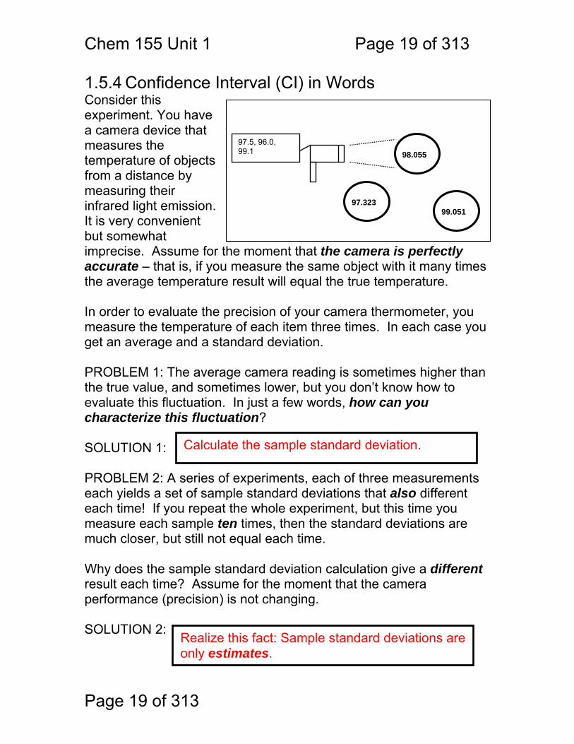
1.5.4 Confidence Interval (CI) in Words Consider this experiment. You have a camera device that measures the temperature of objects from a distance by measuring their infrared light emission. It is very convenient but somewhat imprecise. Assume for the moment that the camera is perfectly accurate – that is, if you measure the same object with it many times the average temperature result will equal the true temperature. In order to evaluate the precision of your camera thermometer, you measure the temperature of each item three times. In each case you get an average and a standard deviation. PROBLEM 1: The average camera reading is sometimes higher than the true value, and sometimes lower, but you don’t know how to evaluate this fluctuation. In just a few words, how can you characterize this fluctuation? SOLUTION 1: PROBLEM 2: A series of experiments, each of three measurements each yields a set of sample standard deviations that also different each time! If you repeat the whole experiment, but this time you measure each sample ten times, then the standard deviations are much closer, but still not equal each time. Why does the sample standard deviation calculation give a different result each time? Assume for the moment that the camera performance (precision) is not changing. SOLUTION 2:

97.5, 96.0, 99.1 98.055

97.323 99.051

Calculate the sample standard deviation.

Realize this fact: Sample standard deviations are only estimates.


Page 20 of 313

1.5.5 CI PROBLEM: This imperfect camera thermometer is going to be used to screen passengers boarding an airliner. Passengers with a high temperature may have avian flu. Our criterion is this: if there is more than a 90% probability that a given passenger’s temperature exceeds 102°, then we will take him aside and test him for bird flu. We have only moments to acquire three measurements per passenger, so precision is low. Also, the precision is not the same each time. For three passengers we get the following results: Passenger 1: 100.3°, 101.1°, 103.0°. Passenger 2: 98.8°, 98.5°, 98.4° Passenger 3: 104.0°, 103.9°, 103.9° How do we answer the question: does this person’s temperature exceed our 90% / 102° criterion? To answer this, we must accept the following: Assuming that measurements are unbiased (accurate) we can state, for the 80% CI, that there is a 10% probability that the true mean lies below the lower limit of the CI, an 80% probability that the true mean lies within this CI, and a 10% probability that the true mean lies above this CI. So, there is a 90% probability that the true mean lies within or above the 80% CI. For example, if we took some measurements and then computed the 80% CI to be 101.8° to 102.6° then we could say that the probability that the true temperature is 101.4° or higher is 90%.

10% chance

μ is 101.8° or lower

101° 102° 103°

80% chance

101.8° < μ < 102.6°

10% chance

μ is 102.6° or higher


Page 21 of 313

Use this table: Use this formula: % confidence interval

°freedom 50 80 95 991 1.00 3.08 12.71 63.662 0.82 1.89 4.30 9.923 0.76 1.64 3.18 5.844 0.74 1.53 2.78 4.605 0.73 1.48 2.57 4.036 0.72 1.44 2.45 3.717 0.71 1.41 2.36 3.508 0.71 1.40 2.31 3.369 0.70 1.38 2.26 3.25

10 0.70 1.37 2.23 3.1720 0.69 1.33 2.09 2.8550 0.68 1.30 2.01 2.68

100 0.68 1.29 1.98 2.63 Complete the following table: Lower

boundaryof 80% CI

Upper boundary of 80% CI

Is the probability that the passenger’s Temp is > 102° 90% or more?

Passenger TAVG(°F) St dev (°F)

1 101.5 1.1 2 98.57 0.17 3 103.93 0.047

CI μ±t s⋅

N⋅

Note the following: For a straight average of N points, the number of degrees of freedom is N-1.


Page 22 of 313

1.5.6 tEXP PROBLEM: Another way of approaching this type of problem is to calculate an experimental value of ‘t’ called tEXP. In the example below, we will compare a measured result with an exact one. The question one answers with tEXP is this: Am I confident that the observed value (x) differs from the expected value (μ)? Our threshold temperature, exactly 102° was tested, so we can make measurements and test the hypothesis that ‘the true temperature is greater than 102°’. Given the following three measurements of a passenger’s temperature: 103.76°, 102.11°, 105.38° – calculate an experimental value of the ‘t’ statistic for this population relative to the true value of 102°. Average = 103.75, std dev = 1.34

% confidence interval °freedom 50 80 95 99

1 1.00 3.08 12.71 63.66 2 0.82 1.89 4.30 9.92 3 0.76 1.64 3.18 5.84

texp103.76 102−( ) 3⋅

1.34:=

texp 2.275= Can you state with the given confidence that this person’s temperature differs from the expected value of 102°? 99%? No 95%? No 80%? Yes 50%? Yes

texpxav μ−( ) N⋅

sμ = test value


Page 23 of 313

ΔS

ΔC= m

0 20 40 60 80 1000

5

10

15

Analyte Concentration (C)

Inst

rum

ent S

igna

l (S)

13.166

0

Si

1000 Ci

1.6 Calibration Curves and Sensitivity

A highly sensitive instrument can discriminate between small differences in analyte concentration.

ΔS

ΔC

≈σS

But, can we really distinguish between small changes in concentration?

Calibration Sensitvity: S = mC + Sb S = instrument signal C = analyte conc. m = slope calibration Sb = signal for blank m = calibration sensitivity

γ = Analytical Sensitvity γ = m / σS γ = (ΔS/ΔC) / σS γ = 1/ΔC for the “ΔC” corresponding to σS

m ≈ and σS ≈ so γ ≈

1 / γ = ‘noise’ in concentration ≈ σC.

So small γ is?

Good

Bad


Page 24 of 313

1.7 Vocabulary: Properties of Measurements Sensitivity A detector or instrument that responds to only a

small change in analyte concentration is sensitive. Numerically, the sensitivity of an instrument is the slope of the calibration curve in untis of: signal / unit concentration – often given as ‘m’. Sometimes the detection limit (see below) is called the instrument sensitivity – but this is not correct.

Selectivity The ratio of the sensitivity of an instrument to an analyte to that of an interferant.

Specimen The material removed for analysis – e.g. a given tablet from an assembly line.

Sample The mixture that contains the chemical to be measured – e.g. the blood sample that we want to measure iron in.

Analyte The chemical that is being measured – e.g. the iron in the blood sample.

Calibration Curve A linear or non-linear function relating instrument response (signal) to analyte concentration.

Interferant Another chemical in the sample that either affects the instrument’s sensitivity to the sample or gives a signal of it’s own that may be indistinguishable from the analyte signal.

Detection Limit CMIN or CM

The minimum detectable concentration of analyte. Usually defined as that concentration that gives a signal of magnitude equal to three times the standard deviation in the blank signal.

Limit of Quantitation (LOQ)

The minimum concentration of analyte for which an accurate determination of concentration can be made. The LOQ is typically that concentration for which the signal is 10x the standard deviation of the blank signal.

Limit of Linearity (LOL) The largest concentration for which a calibration curve remains linear.

Linear Dynamic Range (LDR)

The range of concentrations (or signal strengths) between the LOQ and the LOL. An instrument is most useful within its’ LDR.


Page 25 of 313

1.8 Detection Limit The detection limit is denoted “CM” CM is the minimum concentration that can be “detected,” or distinguished confidently from a blank. Let us define the minimum detectable signal change as: ΔSM Therefore: ΔSM = mCM must be a multiple (n) of the noise level in the blank: (σb).

By convention, m=3. Derive a formula for CM based on σB and m:

Derive a formula for CM based on γ :

γ = m/σ so 1/γ = σ/m CM = 3σ/m = 3/γ

ΔSM ≡ 3σb = mCM

Minimum Detectable Signal

Signal due to blank

mCM = 3σb so

CM = 3σb/m

Minimum detectable concentration


Page 26 of 313

1.8.1 A Graphical Look at Detection Limit (CMIN)

Consider the minimum detectable signal in the context of the confidence interval: SMIN = 3σb + Sb To what confidence interval does 3σ correspond? Assume N=2 (two replicate measurements of Sb) Another way of saying this (crudely) is that we consider a signal ‘detected’ when it falls outside of the boundaries corresponding to the 99.7% confidence interval for the blank signal.

zσ/N1/2 = 3σ z/N1/2 = 3 z = 3*11/2 = 3 z = 3 corresponds to the 99.7% confidence interval


Page 27 of 313

1.8.2 Minimum Detectable Temperature Change? Using the thinking that we developed for the general case of signals with random error – what do you think is the probability that the following signal change is due to random fluctuations?


Page 28 of 313

1.8.3 Dynamic Range LOQ = Limit of Quantitation (σS/S ≈ 0.3) LOL = Limit of Linearity

Between LOQ and LOL your instrument is most useful! This is called:

Linear Dynamic Range


Page 29 of 313

1.8.4 Selectivity Sometimes another chemical species will add to or subtract from your analyte signal – S = mACA + mBCB + mCCC + mDCD + … + SB Selectivity coefficients determine how serious an interferant is to your determination of analyte CA: kB,A = mB/mA, kC,A = mC/mA, etc… So: S = mA(CA + kB,ACB + kC,ACC + …) + SB

Analyte Interferants Blank


Page 30 of 313

1.8.5 Direct Interference In order to measure a concentration directly, without corrections, kB,A, kC,A must be approximately: If there is interference, it is necessary to know both: and before one can determine the desired quantity CA!

Zero!

kB,A, kC,A

CB, CC


Page 31 of 313

1.9 Linear Regression Least-Squares Regression or Linear Regression

Assuming that a set of x,y data pairs are well described by the linear function y = a+bx, and assuming that most error is in y (x is more precisely known) and the errors in y are not a function of x, then the coefficients that minimize the residual function:

χ2 = Σ(yI – (a + bxI))2 can be found from the following equations:

from Data Reduction and Error Analysis for the Physical Sciences, Philip R. Bevington, cw. 1969 Mc Graw Hill.

Non-linear Regression

Methods for fitting arbitrary curves to data sets.

Standard Additions Plot

A nearly matrix-effect free form of analysis. A standard additions plot is a linear plot of instrument signal versus quantity of a standard analyte solution ‘spiked’ or added to the unknown analyte sample. The unknown analyte concentration is derived from the concentration axis-intercept of this plot.

Sample Matrix / Standards Matrix

The matrix is the solution, including solvent(s) and all other solutes in which an analyte is dissolved or mixed

Matrix Effect A matrix effect refers to the case where the instrumental sensitivity is different for the sample and standards because of differences in the matrix.

Internal Standards A calibration method in which fluctuation in the instrument signals due to matrix effects are, ideally, cancelled out by monitoring the fluctuations in the instrument sensitivity to chemicals, internal standards, that are chemically similar to the analyte.


Page 32 of 313

0 2 4 6 8 100

0.5

1

1.5

Analyte Concentration (C)

Inst

rum

ent S

igna

l (S)

1.5

0

Si

Si

FiFi

100 Ci

1.9.1 Linear Least Squares Calibration The most common method for determining the concentration of an unknown analyte is the simple calibration curve. In the calibration curve method, one measures the instrument signal for a range of analyte concentrations (called standards) and develops an approximate relationship (mathematically or graphically) between some signal ‘S’ and analyte concentration ‘C’. If the signal-concentration relationship is linear, then: But, one can not just draw the line between any two points because all the points have some error. So, one mathematically attempts to minimize the residuals.

χ2 = Σ(yi – (a + bxi))2

S = SB + mC y = a + bx


Page 33 of 313

The values of a and b for which χ2 is a minimum are the following: The errors in the coefficients, σa and σb can be found, similarly, using:

These quantities are best found using a computer program. Modern versions of Microsoft Excel will calculate a and b for you (use ‘display equation’ option on the ‘trend line’), and σa and σb if you have the data analysis ‘toolpack’ option installed. Excel is also fairly well suited to doing the sums and formulas.


Page 34 of 313

See also, appendix a1C in Skoog, Holler and Nieman. But, be advised that there is a typo in older editions. Equation a1-32 should read:

m = SXY/SXX Also – it is a somewhat more subtle problem to calculate the error in a concentration determined from a calibration curve of signal (y) versus concentration (x). You will need to follow Skoog appendix-a calculations to deal with this problem in your lab reports where you determine an unknown concentration. M = the number of replicate analyses, N = the number of data points. Note: when computing a confidence interval using this sC value, the degrees of freedom are N-2. (See for example Salter C., “Error Analysis Using the Variance-Covariance Matrix” J. Chem. Ed. 2000, 77, 1239.

Equation a1-37Skoog 5th edition. sc

sym

1M

1N

+ycavg yavb−( )2

m2 Sxx⋅+⋅


Page 35 of 313

1.10 Experimental Design: Designing an experiment involves planning how you will: make calibration and validation standards; prepare the sample for analysis; and perform the measurements. 1.10.1 Making a set of calibration standards.

1. You need to know the dynamic range of your instrument.

2. You need to know the sample size requirement of your instrument.

3. You need to know the estimated expected concentration of your sample.

4. You need to prepare and dilute your sample until it is a. within the dynamic range of your instrument and b. such that there is enough solution to measure.

5. You need to choose target standard concentrations that bracket the expected sample concentration generously – e.g. by a factor of 2 to 3. For example, if your expected concentration is 5.3 ppm, you may wish to make a calibration set that consists of standards that are about 2,4,8,10 and 12 ppm.


Page 36 of 313

6. You need to make a primary stock solution, the concentration of which you know accurately and precisely. This solution will usually be more than twice as concentrated as your most concentrated calibration standard. You will dilute this primary stock solution to make the calibration standards. You need to have enough to make all of your calibration standards.

7. You need to choose the pipets and volumetric flasks that you will use to perform the dilutions. This means that you plan the preparation of each standard. This takes some planning and compromising and many choices – there are many ways to do this correctly – there is more than one right answer!

8. Decide on and record a labeling system in your notebook, collect the glassware, and do the work. I have a labeling system for your caffeine, benzoic acid, iron and zinc standards – I need you to use these labels so that we can sort things out in the class.


Page 37 of 313

1.10.2 Exercise in planning an analysis: Assume that you will be analyzing sucrose in corn syrup sweetened ketchup packets. The packets are thought (i.e. expected) to contain about 0.8 grams of corn syrup that is about 70% sucrose by weight. The HPLC instrument that you will be using can detect sucrose by refractive index in the 0.1-20 parts per thousand (ppth) range (this is the instrument’s dynamic range for sucrose). You have pure sucrose for standards, and will be making five calibration standard solutions. The instrument requires between 250 and 1000 μL of sample. You have the following glassware at your disposal: Pipets Volumetric Flasks Volume Relative

Precision Volume Relative

Precision 20-200 μL 5-1% 1 mL 1% 1 mL 1% 5 mL 1% 5 mL 1% 10 mL 1% 10 mL 1% 25 mL 1% 15 mL 1% 50 mL 1% 20 mL 1% 100 mL 0.5% 25 mL 0.5% 250 mL 0.5% 50 mL 0.5% 1000 mL 0.25%


Page 38 of 313

1.10.3 Plan the analysis!

1. If you dissolve the packet in water, dilute it to 100.0 mL and filter it, what will the approximate sucrose concentration be (ppth)?

0.8 g syrup

0.7 g sucrose 1

1000 mg sucrose

1 mL water

= 5.6 ppth

g syrup 100 mL water g sucrose

1 g water

Is this within the dynamic range? Would it be better to use 10, 25 or 50 mL of water?

2. You need to prepare a stock solution of sucrose

to make the calibration standards. What concentration should this stock solution be? 1, 10, 100 or 1000 ppth?

3. How much sucrose would be required to make: 1, 10, 100 or 1000 mL of this solution?

1.0 mL

100 mg sucrose

=

100 mg sucrose =

0.100 g sucrose

1 mL

soution

10 mL =>

1.00 g sucrose

100 mL

=>

10.0 g sucrose


Page 39 of 313

1.10.4 How to make primary stock solution:

1. Weigh out the desired quantity of pure (e.g. dry,

or oxide-free) analyte material. 2. Dissolve this amount quantitatively, i.e. without

any loss, in the desired solvent. 3. Transfer this liquid quantitatively into the

desired volumetric flask. 4. Dilute to volume with the desired solvent – this

process is important! It is often poor practice to add 5 mL of ‘a’ to 5 mL of ‘b’ and anticipate that the final volume will be exactly 10 mL!

Remember the words DILUTE TO VOLUME!


Page 40 of 313

4. What concentrations ‘bracket’ the 5.6 ppth

target? For example:

5.2, 5.4, 5.6, 5.8, 6.0 ppth --- or --- 1, 2, 4, 6, 8 ppth --- or --- 1, 2, 5, 10, 15 ppth --- or --- 0.050, 0.50, 5.0, 50, 500 ppth

5. What volumes of standards should you prepare? How much is needed by the instrument? What is the smallest volume that you can conveniently and precisely measure? How expensive is the analyte and solvent? How expensive is it to dispose of the waste?

0.1 or 1 or 10 or 100 or 1000 mL

Do you need to make standards on an even spacing?

Does the analyte have to fall right in the middle of the calibration standards?

No, but it minimizes error!

No – but calibration points above and below the std. are needed.


Page 41 of 313

6. How do you prepare the calibration series from

the primary stock solution? Primary Stock (1) is diluted to make Calibration Standard (2) C1V1 = C2V2 First calibration standard: 10 mL of 1 ppth sucrose from 100 ppth stock solution. C1 = 100 ppth C2 = 1 ppth V2 = 10.0 mL V1 = ? = volume to pipet over

V1 = C2V2/C1


Page 42 of 313

7. How to plan a set of standard preparations in the

MS Excel spreadsheet program: Calibration Standard Preparation:Target Conc: Stock Conc: Final Volume: Volume to Pipet:C2 / ppt C1 / ppt V2 / mL V1=C2*V2/C1

1.00 100.0 10.00 0.100 mL2.00 100.0 10.00 0.200 mL5.00 100.0 10.00 0.500 mL

10.00 100.0 10.00 1.000 mL15.00 100.0 10.00 1.500 mL

Calibration StandTarget Conc: Stock Conc: Final Volume: Volume to Pipet:C2 / ppt C1 / ppt V2 / mL V1=C2*V2/C11 100 10 =A4*C4/B4 mL2 100 10 =A5*C5/B5 mL5 100 10 =A6*C6/B6 mL10 100 10 =A7*C7/B7 mL15 100 10 =A8*C8/B8 mL These are formulas that you type into Excel – normally only the result of the formula calculation is displayed.


Page 43 of 313

1.11 Validation – Assurance of Accuracy: Calibration and linear regression optimizes the precision of a calibration curve determination but a calibration curve can only be said to be accurate if: Another way of saying this is that a method is valid if: Validation addresses the various aspects of an analysis that can ‘go wrong’ and give you a wrong answer. The table below lists some of the aspects of an analysis that can be invalid, and suggests ways to validate them. Source of bias: Possible Solution(s): Analyst erratic Analyst can repeat experiment Error in analyst technique

Different analyst does same analysis and gets same result.

Calibration standards are in error (are not what they say the are)

Entire analysis repeated with indpendent calibration standard set

Independent standard measured periodically - called validation standard or QC standard (quality control)

Calibration method

Different calibration method used (standard additions)

Instrument function erratic

Different instrument used (can be a different kind of instrument)

Instrument drift Periodically measure validation standard or internal standard

the analysis has been validated

all significant sources of bias have been removed


Page 44 of 313

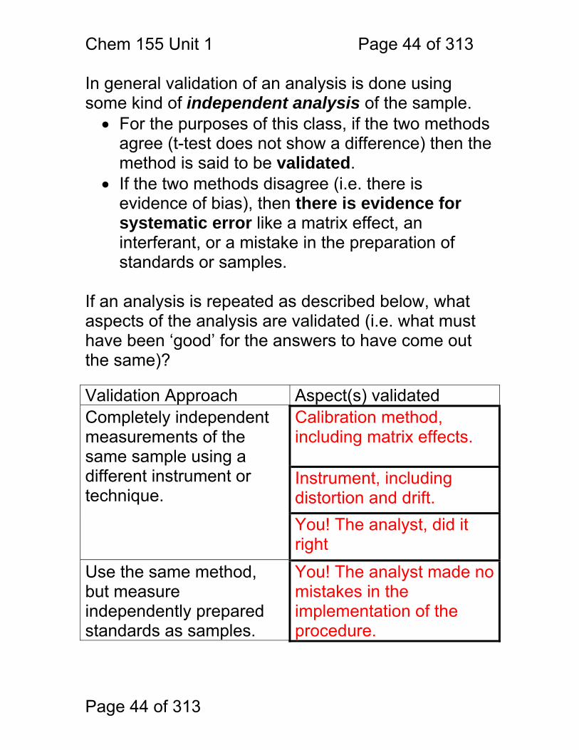
In general validation of an analysis is done using some kind of independent analysis of the sample.

• For the purposes of this class, if the two methods agree (t-test does not show a difference) then the method is said to be validated.

• If the two methods disagree (i.e. there is evidence of bias), then there is evidence for systematic error like a matrix effect, an interferant, or a mistake in the preparation of standards or samples.

If an analysis is repeated as described below, what aspects of the analysis are validated (i.e. what must have been ‘good’ for the answers to have come out the same)? Validation Approach Aspect(s) validated Completely independent measurements of the same sample using a different instrument or technique.

Calibration method, including matrix effects. Instrument, including distortion and drift. You! The analyst, did it right

Use the same method, but measure independently prepared standards as samples.

You! The analyst made no mistakes in the implementation of the procedure.


Page 45 of 313

1.12 Spike Recovery Validates Sample Prep. To do a spike recovery analysis, one takes replicate samples and to a subset of them adds a spike of analyte before the sample prep begins. So, for example, one could take four vitamin tablets, and divide them into two groups of two. To one group one could add some Fe, say half the amount originally expected. For example, if there is supposed to be 15 mg of iron in the tablet, one could spike two samples each with 5 mg of iron and leave two unspiked.

digest filter

Dilute to 100 mL volume

Sample

Sample+ 5.00 mg spike

Analyze 140

ppm 14.0 mg found

digest filter


Analyze 187

ppm 18.7 mg found

18.7-14.0 = 4.7 mg of spike found: spike recovery percent = 4.7 / 5.00 94%

Acids etc.

What does this say about our sample preparation method?

We may be losing about 6% of the analyte during sample prep.


Page 46 of 313

1.13 Reagent Blanks for High Accuracy: A reagent blank is a blank that is made by doing everything for the sample prep etc. but without the sample:

In this example the reagent blank is analyzed against ultrapure water. The 0.23 mg Fe found in the reagent blank may be due to Fe impurities in the acids, but it also may be a matrix effect. In either case, it suggests that we should do what in order to arrive at a more accurate result?

digest filter


“No Sample” sample.

Ultrapure water blank

Analyze 2.3

ppm0.23 mg Fe found

Acids etc used in sample prep.

Either: a. analyze all standards and samples against reagent blanks or b. subtract the signal from the reagent blank against result from sample results made with pure water blanks!


Page 47 of 313

1.14 Standard additions fix matrix effects: Use the method of standard additions when matrix effects degrade the accuracy of the calibration curves. There is one important assumption built into the calibration curve idea. That assumption is the following: Why would the sensitivity be different? 1. Many Instruments are sensitive to things like: 2. Sometimes other chemicals can change the

calibration sensitivity by: These two things are examples of:

the sensitivity of the instrument to the analyte in the standards is

the sensitivity of the instrument to the analyte in the sample matrix

EQUAL TO

1. pH 2. ionic strength 3.organic components of the solvent matrix

chemically binding to or interacting with the analyte atom/molecule

Matrix Effects


Page 48 of 313

1.14.1 How does one deal with matrix effects? 1. Make the sample and standard matrix as nearly

identical as possible: But – matrix matching requires that you already know a lot about your ‘unknown’ – often not the case. So, the matrix-immune alternative to the calibration curve is to: 2. Use the method of: standard additions: In other words, the assumption built into the calibration curve method is that the matrix effects are negligible or identical for standards and samples. If this can not be assumed, one must match the sample and standard matrices. The way that the method of standards additions does with this is to dilute both standards and samples:

matrix matching

in the same matrix (solution)


Page 49 of 313

1.14.2 An Example of Standard Additions: 1. The analyte sample is split up into e.g. 6 aliquots of

identical, known volume – e.g. 1.00 ml. 2. To each of these, a known quantity of standard

(known as a spike) is added – e.g. 0, 0.1, 0.2, 0.3, 0.4, 0.5 ml – standard is dissolved in known matrix like water or 0.1M pH 7 phosphate etc.

3. Each aliquot is diluted to a total volume.

Note: you split and dilute your sample – how does this impact the precision of your measurement?

It decreases it! If volume change is big.

How does this process impact the accuracy of your measurement?

It increases it!

3. Dilute to volume, and mix mix mix!

2. Add standard

1. Add sample


Page 50 of 313

1.14.3 Calculating Conc. w/ Standard Additions: One way of analyzing this uses similar triangles: a / b = The y-axis absorbance signal (S) is proportional to the moles of analyte (VXCX) and standard (VSCS). The x-axis is simply the standard ‘spike’ volume. The x-intercept is the hypothetical spike volume (VS)0 containing the same amount of analyte as the sample. a is proportional to moles of analyte in the sample = VXCX a’ is proportional to moles of std added = VSCS b is (VS)0 – the x-intercept of the graph b’ is VS – the spike volume Substitute for a,a’,b,b’: Solve for CX:

a

b

a'

b'

(VS)0

CX = CS(VS)0/VX

a’/b’

VSCS

= VXCX

VS


Page 51 of 313

1.14.4 Standard Additions by Linear Regression: Let:

VX = volume of unknown analyte solution added to each flask CX = concentration of unknown solution VT = final, diluted volume VS = volume of ‘spike’ added to unknown soln. before dilution CS = concentration of analyte in spike solution

Dilution Calc 1: (V1C1 = VTCT CT = V1C1/VT)

Contribution to concentration of analyte from sample: Dilution Calc 2:

Contribution to concentration of analyte from spike: Total Signal (sensitivity = k) given that ‘x’ variable is CS. S = k + k Slope = m = intercept = b = we can get b and m from linear regression and we want CX … so … b/m = = so : CX =

VXCX/VT

VSCS/VT

VXCX/VT VSCS/VT

kCS/VT

kVXCX/VT

kVXCX/VT kCS/VT

VXCX/CS

bCS mVX


Page 52 of 313

1.15 Internal Standards Internal standards can correct for sampling, injection, optical path length and other instrument sensitivity variations. An internal standard is a substance added (or simply present) in constant concentration in all samples, and standards. When something unexpected decreases the sensitivity of the instrument (m) so the signal drops (S = mC + SB) – it can be impossible to distinguish this from a change in analyte concentration without an internal standard. Consider the ratio of the blank corrected analyte ( BANAN sSS −=' ) to the

internal standard (IS) signals (S): IS

AN

ISIS

ANAN

IS

AN

CCk

CmCm

SS

==''

Assumes for the moment that k is a constant, i.e. invariant to factors affecting overall instrumental sensitivity. As an example, let’s consider k to be a correction for injection volume in a chromatographic system. It is perfectly reasonable to assume that an accidentally low or high injection volume would affect the internal standard and analyte signals identically – e.g. if a given injection were 6% high, then both analyte and internal standard peaks would be 6% larger than expected. If k is invariant to instrument fluctuations, then the true analyte concentration can always be derived from the ratio of the corrected signals so long as the internal standard concentration remains constant.

kSCSC

IS

ISANAN '

'= where

kCIS is easily derived from a previously measured

calibration standard for which the analyte signal ( STDAS −' ) and concentration ( STDAC − ) of the analyte and internal standard

( STDISSTDIS CS −− ,' ) are known: IS

AN

STDASTDIS

STDISSTDA

mm

CSCSk ==

−−

−−

''

From a calibration standard.

Anlalyte conc. in a sample.


Page 53 of 313

In other words, if CIS is held constant in all experiments, then the ratio of the analyte to internal standard signals will be independent of instrument sensitivity. When to use an internal standard? When substantial influence on instrument sensitivity is expected due to variation in things like: Sample matrix Temperature Detector sensitivity Injection volume Amplifier (electronics) drift Flow rate An internal standard must:

a. not interfere with your analyte b. ideally have the same dependence on the chemical matrix,

temperature (or other troublesome variable) as the analyte. Consider the ubiquitous ‘salt plate’ IR sampling method. A drop of analyte is sandwiched between two salt plates and this is placed in the IR beam. The path-length is highly variable from experiment to experiment. The signal A = εbC where ε is characteristic of the molecule, b is pathlength and C is concentration. If you are doing an experiment to measure the increase in amide formation versus time by the intensity of the amide bands near 1700 cm-1. You could take samples and measure them periodically, but the variability of the pathlength would distort the results. On the other hand, if all the samples were spiked with the same amount of acetonitrile then the sharp nitrile stretch at 2250 cm-1 could be used as an internal standard.


Page 54 of 313

1.15.1 Internal Standards Example: In HPLC the sample is injected into a flowing stream, and the signal is a peak in a plot of absorbance versus time (a chromatogram). Often the volume of the injection will vary from injection to injection, so the peaks will vary in size! All

0 400 800 1200 1600 2000 2400 2800 3200 3600 40000

0.5

1

time / s

abso

rban

ce

0 400 800 1200 1600 2000 2400 2800 3200 3600 40000

0.5

1

time / s

abso

rban

ce

0 400 800 1200 1600 2000 2400 2800 3200 3600 40000

0.5

1

time / s

abso

rban

ce

Peak 5 is the analyte, a caffeine standard, 25 ppm, 530 mAu.s

Peaks 2, 3 and 4 are other ingredients in the sample.

Chromatogram 1 is a standard. Did the caffeine concentration increase from chromatogram 1 to 2? Did the caffeine concentration increase in chromatogram 1 to 3?

1

2

3

Peak 1 is the internal standard. 100 ppm NaNO3, 480 mAu.s

100 ppm NaNO3, 520 mAu.s

Unknown caffeine conc. 630 mAu.s


Page 55 of 313

1.15.2 Internal Standards Calculation How about calculating the actual concentration of the sample in 3 above?

Standard

STDAS −' 530 mAu.s

STDAC − 25 ppm

STDISS −' 480 mAu.s

STDISC − 100 ppm

IS

AN

STDASTDIS

STDISSTDA

mm

CSCSk ==

−−

−−

'' 530 100⋅

480 25⋅4.417= unitless

Sample

ANS ' 630 mAu.s

ISS ' 520 mAu.s

ISC 100 ppm

kSCSC

IS

ISANAN '

'= 630 100⋅

520 4.417⋅27.4= ppm


Page 56 of 313

2 Propagation of Error Skoog Chapters Covered: Appendix a1B-4 a1B-5 and – eqn. a1-28 table a1-5 There is a general problem in experimental science and engineering: How to estimate the error in calculated results that are based on measurements that have error? Let’s consider the sum of two measurements a and b that both have some fluctuation sa = 0.5 lb and sb = 0.5 lb. Let’s also pretend that we know the true values of a and b. True value of: a = 5.0 lb

b = 5.0 lb Let’s say that we are weighing a and b and putting them into a box for shipment. We need to know the total weight. Our scale is really bad (poor precision, lots of fluctuation), and it can’t weigh both a and b at the same time because it has a limited capacity. So, we have to first weigh a, then b and then calculate the total weight. But we know that there is a problem with fluctuations, so we repeatedly weigh the same items a and b and do the following experiment:

Characteristics of numbers in sum ‘a’ and ‘b’

Characteristics of sum ‘c’

Trial # Weight of: Deviation: Total weight:

Deviation from avg: A b da db

1 4.5 4.5 -0.5 -0.5 9.0 -1 2 5.5 4.5 +0.5 -0.5 10.0 0 3 4.5 5.5 -0.5 +0.5 10.0 0 4 5.5 5.5 +0.5 +0.5 11.0 +1 average 5.0 5.0 0.5 0.5 10 0.5 This is somewhat artificial and is not quite right, but it gives you the general idea. Errors in a and b propagate into c.


Page 57 of 313

From this example above, one would conclude that the fluctuation in the sum is equal to the fluctuation in the numbers summed – but this is not right. Which is bigger?

a. the fluctuations in the individual numbers summed b. the fluctuations in the sum

Graphically we consider here a similar case, for clarity we let a have a slightly larger fluctuation than b. a = 5 ± 2, b = 3± 1

“Rea

l” d

istri

butio

n

th

eore

tical

th

eore

tical

c

a+sa

a-sa

a+sa+b+sb

a+sa+b-sb

a-sa+b+sb

a-sa+b-sb

a


Page 58 of 313

0 2 4 6 8 100

500

1000

a_dist j 1,

b_dist j 1,

c_dist j 1,

a dist j 0 b dist j 0, c dist j 0,

c_dist histogram 40 c,( ):=

b_dist histogram 40 b,( ):=0.52 0.52

+ 0.707=a_dist histogram 40 a,( ):=

stdev c( ) 0.712=stdev b( ) 0.504=stdev a( ) 0.498=

mean c( ) 6=mean b( ) 2.996=mean a( ) 3.004=

c

0

01

2

3

4

6.3345.991

4.744

6.006

6.005

=b

0

01

2

3

4

3.5543.331

1.98

3.482

3.848

=a

0

01

2

3

4

2.7812.66

2.763

2.524

2.157

=

c a b+:=b rnorm 10000 3, 0.5,( ):=a rnorm 10000 3, 0.5,( ):=

error propagation through sums:


Page 59 of 313

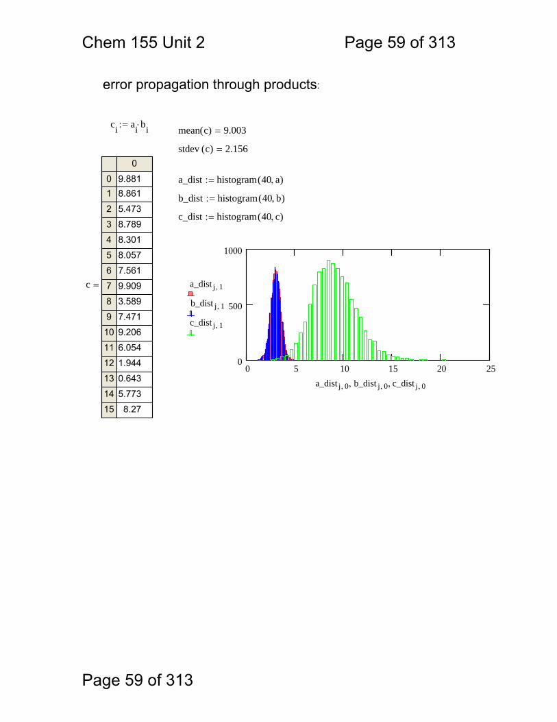
error propagation through products:

ci ai bi⋅:= mean c( ) 9.003=

stdev c( ) 2.156=

a_dist histogram 40 a,( ):=

b_dist histogram 40 b,( ):=

c_dist histogram 40 c,( ):=

0 5 10 15 20 250

500

1000

a_dist j 1,

b_dist j 1,

c_dist j 1,

a_dist j 0, b_dist j 0,, c_dist j 0,,

c

0

01

2

34

5

6

78

9

10

1112

13

1415

9.8818.861

5.473

8.7898.301

8.057

7.561

9.9093.589

7.471

9.206

6.0541.944

0.643

5.7738.27

=


Page 60 of 313

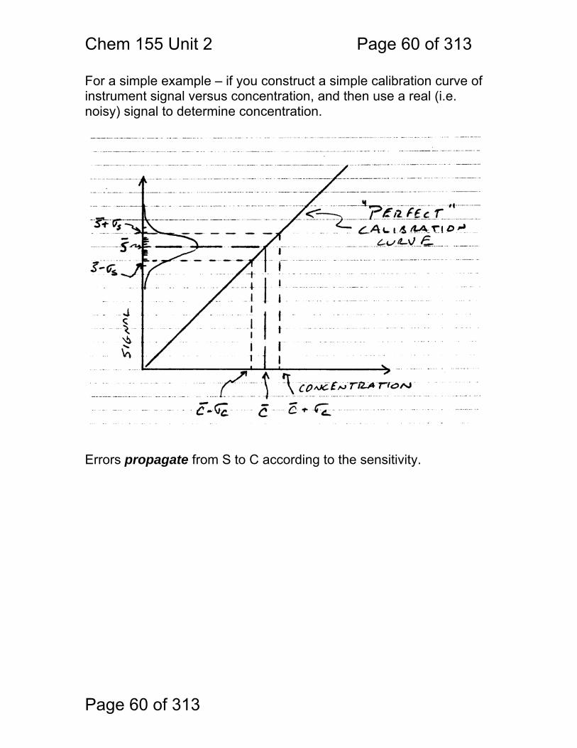
For a simple example – if you construct a simple calibration curve of instrument signal versus concentration, and then use a real (i.e. noisy) signal to determine concentration.

Errors propagate from S to C according to the sensitivity.


Page 61 of 313

Let’s consider an example wherein the relationship between the measured signal and the desired quantity is non-linear :

Obviously – the same error in P can give rise to different errors in A! This is a propagation of error problem. How can you calculate the error in A that should result from a particular error in P?

Absorbance

Absorbance is a nonlinear function of light power - the measured quantity in a spectrophotometric experiment.

A logPP l

0 0.1 0.2 0.3 0.4 0.5 0.6 0.7 0.8 0.9 10

0.5

1

1.5

2

Ai

Pi

A = -log (P/Po)


Page 62 of 313

Obviously, the answer has to do with the way that the dependent variable (A) in this case changes as a function of the independent variable (P). Consider a calculated value ‘S’ that depends on the measured quantites, e.g. instrument signals, a,b,c…

S = f(a,b,c…) In fact – the variance in S is proportional to the variance in a,b,c – and the proportionality is the partial derivative squared: (Skoog appendix a1B-4 has a derivation if you are curious)

So – let’s take an example: S = a+b-c find σS = f(S,a,σa, b,σb,c,σc) Note that the larger terms dominate!

S f a±σa b±σb, c±σc,( )for:

σS2 δS

δa⎛⎜⎝

⎞⎟⎠

2σa

2⋅

δSδb

⎛⎜⎝

⎞⎟⎠

2σb

2⋅+

δSδc

⎛⎜⎝

⎞⎟⎠

2σc

2⋅+


Page 63 of 313

Exercise: Prove the “multiplication / division rule” Show that for S = a*b/c

σ S2

S2

σ a2

a2

σ b2

b2

σ c2

c2


Page 64 of 313

The propagation of error rules for special cases:

Documents

Chemistry 155 Introduction to Instrumental … Lecture 2009...Chem 155 Unit 1 Page 1 of 313 Page 1 of 313 Chemistry 155 Introduction to Instrumental Analytical Chemistry Unit 1 Spring