Embed Size (px)
Citation preview

Chemical Kinetics: Rate and Mechanistic
Models
(CHE 505)
M.P. Dudukovic
Chemical Reaction Engineering Laboratory
(CREL),
Washington University, St. Louis, MO

ChE 505 – Chapter 4N Updated 01/28/05
CHAPTER 4. Chemical Kinetics: Rate and Mechanistic Models 4.1 Introduction By listing the plausible reaction stoichiometries, we can calculate the composition of the system in its final state, i.e. at equilibrium, provided that we are given the thermodynamic properties such as heats (enthalpies) of formation, Gibbs free energies of formation, temperature and pressure of the system, as well as the composition of its initial state. As important as this may be, it does not tell us at all how long will it take for the system to transit from its initial to the final state. Chemicals kinetics deals with the rates of chemical reactions and with how these rates are affected by the composition of the system, temperature and pressure. Kinetic studies are important, since based on them empirical and semi-empirical rate expressions are obtained which then can be used for predictive purposes in analysis of system's dynamic behavior or in design of chemical reactors. Kinetic studies deal with reactions of wide variety of characteristic times. Reactant half-life can vary from a pico- second to a period longer than the age of the universe. Reaction speed will often depend on the conditions of the system. For example, O2 and H2 at room temperature and pressure left alone at stoichiometric ratio for water production would have a half-life of 1025 years or 3 x 1032 seconds. However, a spark causes the half-life to be reduced to 10-6 s! In summary, the scope of kinetic studies is to quantify the rate of reaction as a function of system intensive properties (composition, temperature, etc.) and to suggest a fundamental theory (if possible) for estimation of kinetic parameters. The knowledge of kinetics can answer many important questions related to the environment: For example,
- how fast a species will disappear in a given compartment discussed in Chapter 3. - how much time it is needed to oxidize a pollutant in treatment facilities - how fast processes take place in natural water, and thus will help understanding aquatic kinetics.
In the next section, we start with the definition of reaction rate and investigate how concentration, temperature and other system properties affect these rates. The rate constants can be calculated in different ways, such as empirically, mechanistically, and by performing molecular and quantum level calculations. In this book, we will focus on estimating these rate constants using empirical and mechanistic approaches. These calculations are provided in a later chapter. The present chapter mainly focuses on how reaction rate can be expressed as a function of system variables. 4.2 Reaction Rate Consider an arbitrary mass of the reaction system in its initial state and place an invisible envelope around all the molecules that comprise that mass. This envelope creates the control volume within it. The control volume of the system should be large enough to contain a statistically significant number of molecules so that the concept of molar concentration is meaningful. The control volume of the system should also be small enough so that there are no spatial gradients of composition or temperature within this volume. Let us assume that we can observe this control volume at time t and count the molecules N j of each species j in it. We repeat the observation at time t + ∆ t when the number of molecules of the same species is N j + ∆ N j . During time ∆ t the number of molecules crossing the boundary of the control volume is negligible compared to the change in molecular form due to reaction within the system. The volume of the system can be evaluated at some time
1

ChE 505 – Chapter 4N Updated 01/28/05
θ (t ≤θ ≤ t + ∆t) so that V θ( )=1
∆ tV t( )dt
t
t + ∆ t
∫ is the mean control volume of the system. (Note that
while the control volume may change the mass within it is constant). We can relate the number of
molecules to the number of moles via Avogradro's constant L, n j =N j
L. (L = 6.022.. x 1023
molecules/mol). Then the rate of reaction (rate of formation) of species j is defined as the number of moles of j produced by reaction per unit time and unit volume of the system and is, therefore, given by
R j =lim
∆ t → 01
V θ( )∆ n j
∆ t=
1V
d n j
d t (1)
Please, note that while our above verbal statement is indeed the general definition of the reaction rate, eq (1) is not - it is subject to the assumptions and scenarios depicted above for an isolated, closed, batch control volume. The point is that the rate of reaction of j is always the change in the number of moles of j per unit time and unit volume of the system caused by reaction, but it is only represented mathematically by eq (1) for a closed batch system without spatial gradients. One should remember that in flow systems, or in macroscopic batch systems with spatial gradients, the number of molecules of a species within an element of volume changes not only due to reaction but also due to species being brought in and out of this element of volume by flow or diffusion. Hence, one must take considerable precautions in obtaining reaction rates from experimental data in order not to attribute rates of other processes to the rate of reaction. Details of including flow and diffusion is consider in later chapters. Our above definition defines reaction rate as an intensive property of the system. If only a single reaction takes place in the system then stoichiometry requires that the rates of various components participating in the reaction are tied as shown by equation (2).
R j
ν j= r (2)
where r is the intrinsic kinetic rate of reaction. Unfortunately, even r is not uniquely defined for a reaction system since stoichiometric coefficients can by multiplied by any arbitrary constant, while the number of moles of j converted per unit time and unit volume, R j, only depends on the conditions of the system not on how stoichiometry is written. Thus when we define, r, it is usually with reference to a given stoichiometry for the reaction. Experience shows that reaction rate is a function of composition, i.e concentrations, temperature, catalyst activity, etc. We will talk about the dependence of rate on concentration in the next section. 4.2.1 Dependence of rate on concentration Often, within a narrow range of composition and temperature, the rate can be correlated with a power law dependence on concentration and an exponential dependence on temperature. Hence, for an irreversible reaction a A + b B → p P with K → ∞ an n-th order rate form is frequently fitted to data r = k o e −E /R T C A
α C Bβ (3)
2

ChE 505 – Chapter 4N Updated 01/28/05
This rate form is a product of a function of temperature with a function of composition. At constant temperature we speak of a (specific) rate constant k = k o e −E /R T where k o is the frequency factor, E is the activation energy, R the ideal gas constant and T absolute temperature. This is an Arrhenius form for the temperature dependence which will be discussed later. The order of reaction with respect to reactant A is α and the order with respect to reactant B is β . The overall reaction order is n = α + β. If we measure concentrations in (mol/L) then the units of the rate constant for an n-th order reaction are {(mol/L)1-ns-1]. For a reversible single n-th order reaction (aA + bB = pP) the rate is given by γβα
pRTE
boBARTE
fo CekCCekr 21 −− −= (4) The rate constant for the forward reaction is RTE
fof ekk 1−= , where Ef is the activation energy for the
forward reaction, and RTEbob
bekk −= is the rate constant for the reverse reaction and Eb the activation energy for the reverse reaction. Reaction order for the forward reaction is n = α + β and for the reverse reaction is γ . At equilibrium the net rate of reaction is zero and the forward rate equals the reverse rate. Hence, the rate form must be compatible with thermodynamics and this requires that
sc
eqBA
p
b
f KCC
Ckk /1=
⎟⎟⎠
⎞⎜⎜⎝
⎛=
βα
γ
(5)
so that p = sγ , a = sα, b = sβ and and
sHEE r
bf∆
=− (6)
where s is the stoichiometric number of the rate limiting step to be discussed later. One should note that reaction rate is a much stronger function of temperature than of concentration. Activation energies are typically in the range of 10 to 60 kcal/mol (about 40 to 250 kJ/mol). For example, for a irreversible second order reaction, with an activation energy of 40 kcal/mol, doubling the reactant concentration quadruples the reaction rate but raising the temperature by 10oC, from 20oC to 30oC, raises the rate almost tenfold (9.66 times). Many reaction rates cannot be fitted by the power law form and more complex forms are required to tie reaction rate, temperature and concentrations. Often when the functional dependence on temperature and composition cannot be separated in a convenient product of two functions, then a reaction order and activation energy cannot be separately defined. For example the simplest rate form of the Hougen-Watson or Langmuir-Hinshelwood type is given by
3

ChE 505 – Chapter 4N Updated 01/28/05
r =
k o e − E 1 / RT C A
K o e − ∆ E / R T + C A
(7)
where are positive constants. Figure 1a illustrates that reaction order cannot be defined as it is readily seen that the apparent reaction order varies between order one (when at small
E 1,∆ E , k o and K o
,AC C A << K o e − ∆ E / RT ) and zero (whenC A >> Ko e − ∆ E / R T ). We also see from Figure 1b that the apparent activation energy varies between E1 at low temperature, when C A >> Ko e − ∆ E / R T, and (E 1 − ∆ E) at sufficiently high temperature when C A << K o e −∆ E/ RT .
r ln r
1/T
EEEapp ∆−≈ 1
11 EEEapp ∆−≈
Figure 1: a) Sketch of rate of eq(7) vs. concentration, b) Plot of the ln r (at fixed vs. reciprocal temperature.
AC
Two additional remarks are in order. The stoichiometry of the reaction for which the rate form, r, is reported should always be clearly stated. Then R j = ν j r and the rate constant for species j is k j = ν j k . Forgetting this multiplier is a frequent source of unnecessary errors. Similarly if the rate form for species i is reported, Ri , the rate for species j is
R j =ν j
ν iR i . (8)
Often in heterogeneous systems it is more practical to utilize rate forms based on unit surface of catalyst,
r ' molm 2 s
⎛
⎝ ⎜ ⎞
⎠ ⎟ , or unit mass of the system, instead of using a rate form r
molL s
⎛ ⎝ ⎜ ⎞
⎠ , that expresses the rate of
change of in moles per unit volume of the system r ' ' mol / kg s( ). One should then incorporate the appropriate conversion of units into the rate constants. In summary, the intrinsic kinetic rate of reaction can be defined as
rate of reaction( ) =change in moles of j caused by reaction( )
stoichiometric coefficient of j( ) unit measure of the system( ) unit time( )
where unit measure of the system can be volume, mass, surface, etc. It is usually the volume for homogeneous reaction. A final word of caution. When one deals with an n-th order reaction the reaction orders with respect to various species are not necessarily related to stoichiometric coefficients unless the reactions are elementary, i.e proceed in one step. We will talk about the elementary reactions later on.
4

ChE 505 – Chapter 4N Updated 01/28/05
We note that in order to evaluate the rate of reaction at given conditions of the system we will need to know the functional dependence of the rate form on composition and temperature. This can be accomplished based on theory or experiments. We will see how far we can get by using the theory for elementary reactions (e.g. those that proceed in one step) to estimate activation energies and reaction order. We will also see how mechanisms, consisting of elementary reactions, can help us derive rate forms for more complex reactions. At the end we will consider establishing rate forms based on experimental evidence, and planning experiments for evaluation of rate forms. Next we need to examine the temperature dependence of the rate form. 4.2.2 Temperature Dependence of Reaction Rates We have already seen that the expression for the reaction rate at fixed temperature may take a relatively simple n-th order form e.g. r = k C A
α C β with α + β = n (3) or it may have a more complex form e.g.
r =k 1 C A
α
K + C A (7a)
In either case the "constants" in the rate expression are functions of temperature. For the n-th order reaction rate, k may not be a rate constant of a particular elementary step of the mechanism. In general it is a combination (product or ratio) of several rate constants of mechanistics steps. The same is true of k 1, in our Langmuir-Hinshelwood kinetic form of equation (7a), while K in the example given above is also a ratio of some rate constants for elementary steps. (When α = 1 the above form is the Michaelis-Menten form for enzyme catalyzed reactions). The engineer's goal often is to find an empirical n-th order rate expression (such as the first form shown above) since such a form can often match the data reasonably well within the experimental accuracy and is easier to use than the complex rate form. It is further assumed that the temperature dependence can be lumped into the dependence of the rate constant k on temperature. Note: the rate constant is only a constant in the sense that it does not depend on concentrations but it is a function of temperature. Furthermore it is widely assumed that the functional form of the rate constant's dependence on temperature is: k = k o e −E /R T (9) where E is called the activation energy for the reaction, k o is the constant independent of temperature (sometimes called frequency factor - a term borrowed from collision theory), R is universal gas constant. Taking logarithms of both sides of the above equation one gets
l nk = l n k o −
ER
1T
or log k = log k o −
ER
1T
x 0.43429log e6 7 4 8 4
5

ChE 505 – Chapter 4N Updated 01/28/05
The customary engineering practice is, therefore, to plot k vs1T
on a semilog plot (k is on the
logarithmic scale and 1T
on the linear). The slope of such a plot can be related to the activation energy.
ER
= 2.3026 x slope
If semilog paper is unavailable, a plot of l n k vs
1T
yields slope =ER
. Furthermore, often it is
suggested to plot the log (rate) vs 1T
at fixed composition. This is convenient since rate data can be
taken at fixed concentrations (e.g in a differential reactor) at various temperatures. Then a plot of log (r)
vs 1T
is made and the slope is related to E / R (see Figure 1).
FIGURE 2a: Arrhenius Plot for an n-th Order Reaction
slope =ln r2 − ln r1
1T2
−1T1
= −ER
slope =ln
r2
r1
1T1
−1T2
=ER10
100
1
0.1
1T2
1T1
r1
r2
1T
→ Linear Scale
rat fixed comp.
However, occasionally a situation presented in Figure 2b is encountered. A single value of activation energy cannot be extracted.
6

ChE 505 – Chapter 4N Updated 01/28/05
FIGURE 2b: Arrhenius Plot for the L-H Reaction
10
100
1
0.1
1T
Linear Scale
2.3 slope =
E1 − ∆ER
2.3 slope =
E1
R
1,000
r at fixed C
This shows that the habit of plotting the logarithm of the rate vs 1T
is a bad one unless one is sure that
the rate form has an n-th order form, i.e that the temperature and composition dependence of the rate are separable. If this is the case, then at fixed concentrations the rate r = koe
− E RTCAα CB
β( ) can be evaluated at two temperatures T 1 and T 2 and the logarithm taken.
log r 2 = log [k o C A
α C Bβ( )] −
ER T 2
x 0.434
log r 1 = log[ k o C Aα C B
β( )] −E
R T 1x 0.434
Thus
log r 2 − log r 1 = logr 2
r 1
=ER
1T 1
−1
T 2
⎛
⎝ ⎜ ⎞
⎠ ⎟ x 0.434
(9a) and
ER
=2.3026 log
r 2
r 1
1T 1
−1
T 2
=ln
r 2
r 1
1T 1
−1
T 2
= slope
as shown in Figure 2a. However if the rate form is complex, as illustrated below and shown in Figure 2b
7

ChE 505 – Chapter 4N Updated 01/28/05
r =k o1 e − E 1 / R T C A
α
Ko e−
∆ ERT + C A
;k 1 = k o1 e − E 1 RT
K = Ko e − ∆ E / RT
then clearly even at fixed composition plotting log (r ) vs 1T
will not yield a straight line.
Indeed an activation energy does not exist for the above rate form. One can only talk about the apparent activation energy E a p p . Usually for gas phase reactions, at high enough temperatures
Ko e− ∆ E
R T >> C A and the apparent activation energy is E a p p = E 1 − ∆ E since the apparent rate
constant is k o1
K oe
−E 1 −∆ E( )
RT . At low enough temperatures K o e − E/ RT << C A and the apparent
activation energy is E a p p = E 1 as shown in Figure 2b.
In conclusion, a plot of log (r ) vs 1T
will yield an activation energy only if the rate is of the n-th order
type. Even then, if as a result of a particular mechanism the rate constant is actually a combination of
constants for elementary steps, for example k =k 1
'
k 2' + k 3
' , this may not be true. It is also misleading to
do this in heterogeneous systems where mass transfer effects (to be shown later) can mask the kinetic activation energy. Clearly, the above method fails for complex rate forms. The advisable procedure is as follows. Once a rate form is identified, evaluate at each temperature all of
the constants that appear in the rate form and plot them individually as log k( ) vs1T
to extract the
activation energy for each of them.
Plotting log r( ) vs1T
often saves time for the engineer but has to be done with due caution.
We have mentioned that it is a custom to expect the constants in any rate form to show an exponential dependence on temperature of the form k = k o e −E /R T . We will now show which theories suggested that particular form. 4.2.2.1 Arrhenius Law Arrhenius considered in 1889 reversible elementary reactions
Ak 1 f⎯ → ⎯ ⎯
k 1b← ⎯ ⎯ ⎯
P with r = k 1 f C A − k 1b C p (10)
He argued that since for an elementary reaction the equilibrium constant is given by
8

ChE 505 – Chapter 4N Updated 01/28/05
K c =k 1 f
k 1b=
C p
C A
⎛
⎝ ⎜ ⎞
⎠ ⎟
eq (11)
and since van't Hoff's equation for the variation of the thermodynamic equilibrium constant with temperature is
d ln Kd T
=∆ HRT 2 (12)
it is reasonable to assume that the rate constants follow the same type of temperature dependence:
d l n k 1 f
d T=
E f
RT 2 (13a) ;d l n k 1 b
d T=
E b
R T 2 (13b)
We recall that
K =a p
a A
⎛
⎝ ⎜ ⎞
⎠ ⎟
eq=
γ p
γ A
⎛
⎝ ⎜ ⎞
⎠ ⎟
eq
C p
C A
⎛
⎝ ⎜ ⎞
⎠ ⎟
eq= K γ K c = e
− ∆ G °RT (14)
∆ G ° = ∆ H ° − T ∆ S ° (15) Integration of the above derivatives for the rate constants, with Ef and Eb kept constant, gives: k 1 f = ko f e − E f /R T ; k 1b = k ob e − E b /RT (16) E f - activation energy for the step forward E b - activation energy for the reverse step k o f, , k o b - frequency factors for the forward and reverse reaction, respectively. In view of the Arrhenius theory, molecules must acquire a certain critical energy level before they can react. E f is the activation energy for the forward step viewed as the difference between the mean energy level of reactant molecules prone to react (i.e in excited state susceptible to reaction) and the mean energy level of other reactant molecules which are not ready to react. Similarly, E b is the activation energy for the reverse step, i.e the difference in mean energy of "excited" product molecules and "base" product molecules. The factor e - E/ R T is the familiar Boltzmann factor (see any physical chemistry book and the chapter on kinetic theory of gases) which yields the fraction of molecules that managed to acquire sufficient energy level above the mean. Substituting eqs. (11) and (15) into eq (14) yields the following form:
K = K γ K c = K γko fk ob
e−
E f − E b( )RT = e
−∆ H o
R T e∆ S o
R (17)
Thus
9
ChE 505 – Chapter 4N Updated 01/28/05
K γ
k o f
k o b= e
∆So
R (17a)
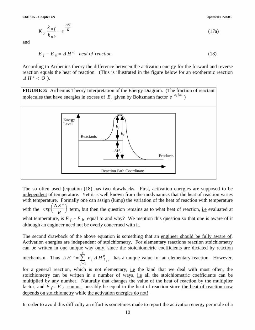
and E f − E b = ∆ H ° heat of reaction (18) According to Arrhenius theory the difference between the activation energy for the forward and reverse reaction equals the heat of reaction. (This is illustrated in the figure below for an exothermic reaction ∆ H ° < O ). FIGURE 3: Arrhenius Theory Interpretation of the Energy Diagram. (The fraction of reactant molecules that have energies in excess of Ef given by Boltzmann factor e− Ef RT )
−∆Hr
Ef
Eb
Products
Reactants
Energy Level
Reaction Path Coordinate The so often used (equation (18) has two drawbacks. First, activation energies are supposed to be independent of temperature. Yet it is well known from thermodynamics that the heat of reaction varies with temperature. Formally one can assign (lump) the variation of the heat of reaction with temperature
with the exp
∆ S °R
⎛ ⎝
⎞ ⎠ term, but then the question remains as to what heat of reaction, i.e evaluated at
what temperature, is E f - E b equal to and why? We mention this question so that one is aware of it although an engineer need not be overly concerned with it. The second drawback of the above equation is something that an engineer should be fully aware of. Activation energies are independent of stoichiometry. For elementary reactions reaction stoichiometry can be written in one unique way only, since the stoichiometric coefficients are dictated by reaction
mechanism. Thus ∆ H ° = ν j ∆ H f j T
o
j =1
s
∑ has a unique value for an elementary reaction. However,
for a general reaction, which is not elementary, i.e the kind that we deal with most often, the stoichiometry can be written in a number of ways, i.e all the stoichiometric coefficients can be multiplied by any number. Naturally that changes the value of the heat of reaction by the multiplier factor, and E f - E b cannot possibly be equal to the heat of reaction since the heat of reaction now depends on stoichiometry while the activation energies do not! In order to avoid this difficulty an effort is sometimes made to report the activation energy per mole of a 10

ChE 505 – Chapter 4N Updated 01/28/05
component, and to require that the heat of reaction be reported per mole of the same component. But activation energies are numbers determined from experiments, while the heat of reaction will again depend if we choose A or B or Q to have a stoichiometric coefficient of magnitude one as shown below. a) 3 A + B = 2Q
b) A +13
B =23
Q
c) 32
A +12
B = Q
If by convention we then require that stoichiometry be written with all stoichiometric coefficients as integers, with no common factor among them, then in the situation above only case a) would be an acceptable representation of stiochiometry. Then
K c( )1/ s =k 1 fk 1b
K c = K / K γ
e∆So
RK γ
⎛
⎝
⎜ ⎜ ⎜
⎞
⎠
⎟ ⎟
e− ∆ H °
RT
⎡
⎣
⎢ ⎢ ⎢
⎤
⎦
⎥ ⎥ ⎥
1/ s
=k o fk o b
e−
E f − E b
RT
and therefore E f − E b =∆ H°
s (19)
where s is the stoichiometric number of the rate determining step. The most useful aspect of the Arrhenius theory is the functional form of the dependence of k on T , i.e k = k o e −E/ RT . However, one should be aware that by assigning such a form to the rate constant irrespective of variables that are used as a "driving force" for the rate (i.e concentration, partial pressure, mole fraction, etc.) the activation energy E, i.e its numerical value, becomes dependent on the choice of variables used in the "driving force". For example consider the rate form for an n-th order reaction:
rmollit s
⎛ ⎝ ⎜ ⎞
⎠ = k c
mollit
⎛ ⎝
⎞ ⎠
1− n
s −1⎡
⎣ ⎢ ⎤
⎦ ⎥ C An mol
lit⎛ ⎝
⎞ ⎠
n
(20)
Suppose then k where E c is the numerical value of the activation energy. c = k co e − Ec
/ RT
If we deal with gas reaction it is often more useful to express the rate as
rmollit s
⎛ ⎝ ⎜ ⎞
⎠ = k p
mollit
⎛ ⎝
⎞ ⎠ atm( )−n s −1⎡
⎣ ⎢ ⎤ ⎦ ⎥ P A
n atm( )n (21)
and the driving force is now expressed in partial pressures.
11

ChE 505 – Chapter 4N Updated 01/28/05
If we now take k p = k po e −E p / RT (and there is nothing in Arrhenius theory to prevent us from doing it) the question arises whether E p = E c , as it should be if the activation energy is a unique number for the reaction. For simplicity we will assume ideal gas behavior PA = CA RT . By comparison of the two rate forms we conclude: k c = k p RT( )n . Then, from the Arrhenius temperature dependence of the rate constants
d ln k cd T
=E c
RT2 ;d ln k p RT( )n[ ]
d T=
E PRT 2 +
nT
we get the following relationship between activation energies E c = E p + n RT (22) The relationship between k c o , and k p o is: (23) k co = k po RT( )n e n
Clearly the value of the activation energy does depend on the quantities used in the driving force term. However, for high activation energies, moderate temperatures (T < 500o K) and reasonable orders of reaction, , the relative error made is usually within 10% which is well within the customary experimental uncertainty in this kind of problems. We will define here
n ≤ 2
relative error = E c − E p
E c=
n RTE c
In spite of all its deficiencies Arrhenius law is used almost exclusively for engineering purposes due to
its simplicity. Thus, Arrhenius plots of l n k vs
1T
are usually made of experimental data, and that is
the simplest and most useful form for engineering work. However, Arrhenius law cannot predict the values of the rate constants even when activation energy is known. This is the ultimate goal of rate theories to be discussed next.
Note: Sometimes rates are given in atm
s⎛ ⎝
⎞ ⎠ especially for gas phase reactions that proceed with the
change in the number of moles, as the change in partial pressure or total pressure is monitored.
?r atms
⎛ ⎝
⎞ ⎠ = k p
' atm( )1−n s −1[ ]P An atm( )n (24)
Then: E c = E' p + (n-1) R T (25) and k co = k p o
' RT( ) n−1 e n−1 for k p' atm 1−n s −1[ ]and k c mol / L( )1−n s −1[ ] (26)
12

ChE 505 – Chapter 4N Updated 01/28/05
Example 1. For the reaction 2NO + Cl2 = 2NOCl
log k c =−803
T+ 3.66 where k c and k c o are in [(lit/mol)2 s-1]
Calculate the rate constant in [torr -2 s-1]. Use 400K as the mean reaction temperature. Note first that n = 3.
E p' = E c − n−1( )RT
E p' = 803
given{ x 1.987
R1 2 3 x 2.3025
conversionof log s1 2 3 − 3−1( )
n−11 2 3
x 1.987R
1 2 3 x 400T
{
E p
' = 3673.8 − 1589.6 = 2084.2calmol
E c = 3674calmol
E p' = 2084
calmol
In reactions with low activation energies the difference in activation energy depending on the choice of units is considerable. The difference above is 43% based on E c.. Now k c o = 103.66 so that
k po
' = k c o ′ R T( )1− n e 1−n
k po' = 103.66 760 x 0.0821 x 400( )1−3 e 1−3
Note that here we needed ′ R in units of (torr L /mol K) and we obtain it by taking R = 0.0821 ( L atm/ mol K ) and multiplying it by 760 (torr/atm). [ ]127' 1093.9 −−−×= storrk po
k c o = 103.66 = 4.57 x 10 3 lit
mol⎛ ⎝ ⎜ ⎞
⎠
2
s −1⎡
⎣ ⎢
⎤
⎦ ⎥
The last example demonstrates that if say k c o, Ec are assumed to be independent of temperature, then k p o
' , E p' and E p would vary with temperature.
The realization that these parameters may indeed be a function of temperature, especially over a broad temperature range, led to the use of the modified Arrhenius equation. k = k o
' T m e −E' / RT (27) The relationship to the usual form of Arrhenius equation k = k o e - E / R T is as follows:
13

ChE 505 – Chapter 4N Updated 01/28/05
RTEm
oo eTkk'' −= (28a)
E = E' + m RT (28b) T is the mean temperature for the range of experiments, E' , k o ' are constants independent of
temperature, m is a parameter proportional to the ratio C p act
Rwhere C p act is the molal heat
capacity for activation. Hence, m is small for gas phase reactions but may be as high as 40 for ionic reactions in solution.
Several times on the last few pages we have presented the relationships between activation energies and frequency factors of the rate constant for different representations of the rate forms. These relationships are the result of simple mathematical manipulations which for completeness are outlined in detail below. Assume that we want to relate the kinetic constants and their activation energies for the rate form expressed by equation (20) and that expressed by equation (24) for the same reaction.
nA
RTEc Cek
sLmolr c /
0−=⎟⎟
⎠
⎞⎜⎜⎝
⎛ (20)
?r atm
s⎛ ⎝
⎞ ⎠ = k po
' e−EP' / RT pA
n (24)
We need an equation of state, in this case the ideal gas law pA = CART. By multiplying equation (20) with RT we convert the form r into as shown below: ?r
rmolLs
⎛
⎝ ⎜ ⎞
⎠ ⎟ RT
atm Lmol
⎛ ⎝
⎞ ⎠ =
?r atm
s⎛ ⎝
⎞ ⎠ (29)
The above equality can be represented by kcoe
− Ec / RTCAnRT = k po
' e− EpRTCAn (RT )n (29a)
Upon canceling the common factors we have (29b) kcoe
− Ec / RT = k po' e−Ep
' / RT (RT ) n−1
We require now that the derivative with respect to temperature T of the natural logarithm of the left hand side (LHS) and the right hand side (RHS) are equal. This is essentially equivalent to requiring that the Van’t Hoffs equation applied to the representation of the rate constant on the LHS and on the RHS is identical. This yields
( )[ ] [ ))(( 1/'/ '−−− = nRTE
poRTE
co RTeknd
]Tdekn
dTd pc ll (30)
14

ChE 505 – Chapter 4N Updated 01/28/05
Ec
RT 2 =Ep
'
RT 2 +n −1
T=
E p' + (n −1)RT
RT 2 (30a)
This yields equation (25) (25) Ec = E p
' + (n −1)RT Now substituting in terms of EEp
'c from equation (25) e.g. Ep
' = Ec − (n −1)RT , into equation (29b) we get kcoe
− Ec / RT = kpo' e−Ec / RT e(n−1) RT( )n−1
(29c) which upon canceling the common factor e− Ec / RT yields equation (26) (26) kco = k po
' (RT )n−1 e(n−1)
Clearly, equations (25) and (26) cannot be satisfied at every temperature! Usually some reference temperature or the mean temperature in the region of interest is used. So these equations hold at T = T . The same procedure is used to relate the rate constants predicted by collision theory and transition state theory, discussed in the next chapter, to the parameters kco and Ec of the Arrhenius form. 4.3 Elementary Reactions For elementary reactions, the one to one correspondence exists between order and molecularity of reaction. Unimolecular reactions are first order, bimolecular are second order, etc. Elementary reactions are those that proceed in one step (a rather loose definition since possibilities of the intermediate on the way from reactants to product is allowed in many theories as we will see later). The stoichiometry of elementary reactions is not arbitrary and the stoichiometric coefficients must be integers reflecting the molecularity of the process. Molecularity of an elementary reaction is identified by the number of elementary particles involved in the event leading to reaction. Molecularity with respect to species j is the number of molecules of that species involved in the event leading to the reaction. Stoichiometric coefficients are now equal to molecularity of the species involved. Only for elementary reactions the law of mass action applies, and the rate of the forward reaction equals the product of reactant concentrations raised to their respective stoichiometric coefficients, (e.g. for A+B P the rate forward is r f = k 1C A C B.). The same rule holds for the reverse reaction (e.g. for
→P → A + B reverse rate is r b = k 2 C P ).
In this section, we will give examples of elementary gas-phase reactions and elementary reactions in solution. Let’s start with gas-phase reactions; we will classify these as unimolecular, bimolecular, and trimolecular. Unimolecular elementary gas-phase reactions:Originally simple decompositions were thought to be elementary unimolecular reactions such as (31) 2 5 2 4 1/ 2N O N O O→ + 2
but this was later proven to be untrue. However, examples of unimolecular (hence first order reactions) do exist such as isomerization of cyclopropane to propylene, dissociation of molecular bromine and
15

ChE 505 – Chapter 4N Updated 01/28/05
decomposition of sulfuryl chloride (i.e ). 2 2 2S O C S O C→ +l l 2
Unfortunately, the original simple hypothesis that unimolecular reactions do not depend on molecular collisions and hence occur only by absorbing energy and forming an activated complex was later disproven by showing that believed unimolecular reactions do not remain first order at very low pressures. Hence, although a unimolecular reaction is supposed by definition to involve one molecule of the reactant species only, and proceed in one step, the definition was broadened to allow mechanisms for explanation of unimolecular reactions. A mechanism is a postulated sequence of elementary steps that leads from reactants to products. Lindemann-Christansen (L-C) Hypothesis asserts the following mechanism for a unimolecular reaction
A P R→ +
R
(32a) 1
1
*k
k
A A A A−
⎯⎯→+ +
←⎯⎯
(32b) 2* kA P⎯⎯→ +
Since [A * ] << [A] its rate of change is very small so that
[ ] [ ][ ] [ ]
[ ] [ ][ ]
2* 1 1 2
21
1 2
* *
*
AR k A k A A k A O
k AA
k A k
−
−
= − −
=+
=
Now from stoichiometry R p = R A - so that
[ ] [ ][ ] [ ]
21 2 1
21 2
*p
k k AR k A k A
k A k−
= = =+
(33)
When pressure is not too low k - 1 [A ] >> k 2 and
[ ] [ ]11 2
1p
k kR A k Ak ∞
−
= = (34)
If pressure is sufficiently low k - 1 [A ] << k 2
[ ] 21pR k A= (35)
and second order is observed. This analysis indicates that the observed rate constant the unimolecular reaction would be pressure,
1ki.e concentration of A, dependent since
[ ][ ]
[ ]
12
1 2 11
21 2
1
1
kkk k A k
k kk A kk A
−
−
−
⎛ ⎞⎜ ⎟⎝ ⎠= =
+ + (36)
The plot of [ ]1
1 vsk A
1 should be a straight line
16

ChE 505 – Chapter 4N Updated 01/28/05
[ ]
11
1 2 1
1 kk k k k A
−= +1 (37)
which unfortunately is not quantitatively confirmed as evident from Figure 4. However the dependence of the "first order" rate constant k 1 on pressure is evident. This means that while Lindemann's theory qualitatively predicts correctly the change in reaction order with pressure it does not explain it quantitatively. However, Lindemann- Cristensen’s theory holds when the proper estimates of the rate constants are arrived at by using quantum mechanics and statistical mechanics calculations as shown in the approach of Rice, Ramsberger, kassel and Marcus ( the RRKM theory). Professor Marcus at Caltech was a Nobel prize recipient. Those interested for a more in debt discussion of unimolecular reactions or RRKM theory should consult the literature ( e.g. W. Frost, ‘Theory of Univmolecular reactions”. FIGURE 4: Schematic plots of 1/k1 versus 1/[A]
1/[A]
Bimolecular elementary gas-phase reactions: Bimolecular gas phase reactions can occur:
- between two molecules - between a free radical and a molecule - between an ion and a molecule - between two free radicals
Kinetic results are also available for bimolecular reactions involving atoms and free radicals. Many of these are abstraction (e.g. metathetical) reactions such as
3 2 6 4 2CH C H CH C H° + → + 5° (38)
For all bimolecular reactions the rate is second order and given by:
/E RTA Br Ae C C−= (39a)
or
(39b) /' PE RTA Br A e p p−=
17

ChE 505 – Chapter 4N Updated 01/28/05
The pre-exponential factor can be estimated from collision or transition state theory as will be discussed later. At that time some typical bimolecular gas phase reactions and values of their kinetic parameters will be presented. Trimolecular elementary gas-phase reactions: The first gas phase reaction of this type that was observed was (40) 22 2NO Cl NOCl+ = Later it was found that indeed all reactions of the type (41) XNOXNO 22 2=+ with , ,X Cl O Br= , etc. are trimolecular and occur in one step. Hence, the rate is third order, second order in NO and first order in X 2. At constant temperature the rate is given by (42) [ ] [ 2
2 XNOkr= ]
] where indicates the concentration of N O and X 2 respectively. Of course the rate can also be represented in terms of partial pressures but overall reaction order is always 3 (three).
[ ] [ 2 and XNO
Combination and Disproportionation Gas Phase Reactions
Examples of these are
- reactions between atoms (43) 2H H H+ →
- reactions between free radicals (44) * *
3 3 2C H C H C H+ → 6
These have essentially zero activation energy and occur due to every collision.
- free radical-molecule reaction (45) *
2 4 2H C H C H+ → *5
6
- disproportionation (46) * *
2 5 2 5 2 4 2C H C H C H C H+ → +
These are not simple bimolecular reactions since they are the reverse of unimolecular reactions and hence have special features. If the rate of the reverse reaction is known or calculable by RRKM theory, then the equilibrium constant can be used to derive the rate form and kinetic constants for the forward reaction. Consider (47a) * *
3 3 2C H C H C H+ → 6
18

ChE 505 – Chapter 4N Updated 01/28/05
[ ]2 62*
3
with c
C HK
C H=
⎡ ⎤⎣ ⎦ (47b)
The reverse decomposition reaction
(47c) *2 6 3C H C H C H→ + *
3
at sufficiently high pressure is 1-st order by LC mechanism:
r-1 = k - 1 [C 2 H 6 ] (48)
At equilibrium it follows that:
(49a) 1 1r r−=
[ ] [ ]1 3 1 2k CH k C Hα−= 6 (49b)
Since
[ ]2 61
*2 3
C Hkk CH
α=⎡ ⎤⎣ ⎦
(49c)
and due to equilibrium equation (47b)
and the fact that we must have 1
2c
k Kk
= , it follows that 2α = . Then,
(50) 2
*1 1 3r k C H⎡ ⎤= ⎣ ⎦
On the other hand at very low pressure the decomposition is 2nd order (due to LC mechanism)
[ ] 2
1 1 2 6r k C H− −= (51)
which implies that
[ ]2*1 1 3 2 6r k C H C H⎡ ⎤= ⎣ ⎦ (52)
The forward rate is now third order. Mechanisms of Atom and Radical Combinations In the dissociation of a molecule R 2 into two radicals R * the initial step is the energization process
*2 2R M R M+ → + (53a)
the second step is the dissociation
* *2 2R R→ (53b)
The initial step (initation) was brought about by a molecule M which may be R 2 or an added substance (third body).
Termination of the free radical R * follows then the reverse of the above process
19

ChE 505 – Chapter 4N Updated 01/28/05
1
1
*22
k
k
*R R−
⎯⎯→←⎯⎯
(54a)
2*2
k2R M R+ ⎯⎯→ + M (54b)
For combination (termination) reactions the third body M is known as the chaperon. The energy of *2R
is transferred to M, which provides the energy transfer mechanism.
Using the fact that the net rate of formation is zero, *2R 30*
2=
RR , the concentration of can be found
as shown below:
*2R
[ ]2* * *1 1 2 2 2 0k R k R k R M−⎡ ⎤ ⎡ ⎤ ⎡ ⎤− −⎣ ⎦ ⎣ ⎦ ⎣ ⎦ = (55a)
[ ]
2*
1*2
1 2
k RR
k k M−
⎡ ⎤⎣ ⎦⎡ ⎤ =⎣ ⎦ + (55b)
The rate of *R termination is twice the rate of 2R formation since the overall stoichiometry is : 2
*2 RR =
[ ][ ]
[ ]
2*1 2*
* 2 21 2
22R
k k R MR k R M
k k M−
⎡ ⎤⎣ ⎦⎡ ⎤− = =⎣ ⎦ + (56)
Hence, at sufficiently high pressures
and [ ]
2
1 2
** 12R
k k M
R k R
− <<
⎡ ⎤− = ⎣ ⎦ (57)
second order termination rate is observed.
At sufficiently low pressures
and [ ]
[ ]1 2
2** 1 22R
k k M
R K k R M
− >>
⎡ ⎤− = ⎣ ⎦ (58)
and third order termination is observed. Here 1 1/K k k 2= is the equilibrium constant for the first step.
Combination and termination of free radicals most likely follows the above mechanism. The combination of atoms represents an extreme situation. If energy transfer applies two atoms will come together and separate within the period of first vibration ~ 10-13 s unless an effective chaperon molecule arrives and collides with the complex within such short a time. Only at gas pressures of 104 to 105 atm are collision frequencies high enough for them to be likely. The combination rates are low and 3rd order. However, an alternative mechanism often plays a role, that is the atom-molecule complexation mechanism.
1
1
*k
k
*R M R−
⎯⎯→←⎯⎯⎯+ M (59a)
20

ChE 505 – Chapter 4N Updated 01/28/05
2
2
* k
kRM M RM M
−
⎯⎯→←⎯⎯⎯+ + (59b)
2*2
kRM R R M+ ⎯⎯→ + (59c) The predicted rate is [ ]2*
* 3 1 22RR k K K R M⎡ ⎤− = ⎣ ⎦ (60) where 111 −= kkK and 222 −= kkK . The kinetics remains third order at all pressures. This mechanism is favored if k1 is large, R M * is a strong complex. How to derive rate forms from postulated mechanism in a systematic way will be discussed in the next Chapter. Elementary reactions in solution Elementary reactions also occur in the liquid phase. They can be reactions between two species dissolved in a solvent or reactions of solute with the solvent. These reactions are quite different from gas phase reactions, since the medium (solvent) is considerably denser and more viscous. The solvent may and may not participate in the stoichiometry of the reaction. In either event, since the concentration of the solvent is much greater than that of the solute reactants, the solvent concentration does not change due to reaction. Some new concepts, yet to be introduced, will be needed, to handle even elementary reactions in solution. This will be postponed for a later chapter, after our treatment of elementary gas phase reactions via collision and transition complex theory. 4.4 Non-elementary Reactions Composite or complex reactions consist of a sequence of elementary steps and speaking of the molecularity for the overall reaction has no meaning. Reaction order and stoichiometry are now unrelated.
Many reactions proceed via chain mechanisms that induce a closed loop catalytic sequence. Catalysts can be generated by initiation steps of the chain reaction or are unchanging species that speed up reaction rates. Inhibition of the rate, i.e slow down, is catalyzed by inhibitors - negative catalysts. We will consider next how to evaluate rate forms for gas phase reactions based on proposed mechanisms consisting of sequences of elementary steps.
21

1
February 9, 2007 Addendum to Chapter 4 For the spontaneous decomposition of ozone triggered by activation caused by UV
radiation, we have seen that the following mechanism is in agreement with the observed
rate form.
O3
k1⎯ → ⎯
k2← ⎯ ⎯
O + O2 (1)
O + O3k3⎯ → ⎯ 2O2 (2)
The overall stoichiometry is
2O3 = 3O2 (3)
The first step, shown is reversible, is essentially the UV triggered initiation step, from left
to right, and extinction (termination) step for the free radical, from right to left.
We have seen that application of PSSA to the above mechanism leads to the following
rate form:
−RO3=
2k1k3CO 32
k2CO2+ k2CO3
(4)
Since the first term in the denominator dominates at most conditions, the rate can be
represented as
−RO3= 2k3K1
CO 32
CO2
(5)
where K1 = k1/k2 is the equilibrium constant for the first step.
Observing our previous result for the concentration of the active intermediate, CO, we
note that
CO = K1CO3
CO2
(6)
so that the rate can be represented by
−RO3= 2k3(CO )(CO 3 ) (7)
which is the rate for step 2, which is the rate-limiting step (RLS).

2
The value of the rate constant is reported as:
k3 =1.9x10⁻¹¹e−2300 / T (cm3 / molecule s) (8)
[Convert this to usual molar units such as (cm3/mol s) or (L/mol s)]
We are interested in estimating by how much can this rate be accelerated in the presence
of the catalyst such as chlorine atoms or radicals that occur in the stratosphere due to the
presence of fluorochlorocarbons like freons.
This catalyzed decomposition of ozone can be represented by a simplified Rowland-
Robinson mechanism
CF2Cl 2
hυ→
< 220nm
Cl + CF2Cl (9)
The above is the initiation step that gives rise to the following catalytic sequence (cycle)
Cl + O3kc1⎯ → ⎯ O2 + ClO (10)
ClO + O kc2⎯ → ⎯ Cl + O2 (11)
The sum of (10) and (11) leads to
O + O3Cl⎯ → ⎯ 2O2 (12)
and we want to compare the rate of the catalyzed ozone decomposition (reactions (10)
and (11)) to step (2) of the uncatalyzed mechanism. It is known that
kc1 = 5x10⁻¹¹e−140 / T (cm3 / molecule s) (13)
kc 2 =1.1x10⁻¹⁰e−2.20 / T (cm3 / molecule s) (14)
Notice the much lower activation energy for the rate constants of the catalyzed steps.
Using PSSA we set the net rate of formation of ClO to zero.
RClO = kc1CClCO 3 − kc 2CClOCO = 0 (15)
Since the sequence is catalytic we recognize that the total concentration of
Chlorine atoms available (Cl and ClO) is constant
CCl + CClO = CClo (16)
3
Since from eq (15) it follows that
CCl =
kc2CO
kc1CO 3
CClO (17)
Upon substitution for CClO from eq(16) into eq (17) we get
CCl =
kC 2COCClo
kc1CO 3 + kc2CO
(17a)
and
CClO =
kC1C03CClO
kc1CO 3 + kc2CO
(17b)
The catalyzed rate of ozone decomposition becomes
−RO3C
= kc1CClCO 3 =k1kc2CCl
o COCO 3
kc1CO3 + kc2CO
(18)
Typically, kc2CO << kc1CO3 so that the rate can be represented by
−RO 3 = kc2CClO CO (19)
Now let us compare the above catalytic rate of ozone decomposition and the spontaneous
rate of eq (2).
−RO 3C
−RO 3
=kc2CCl
O CO
k3COCO 2
=kC 2CCl
O
k3CO3
(20)
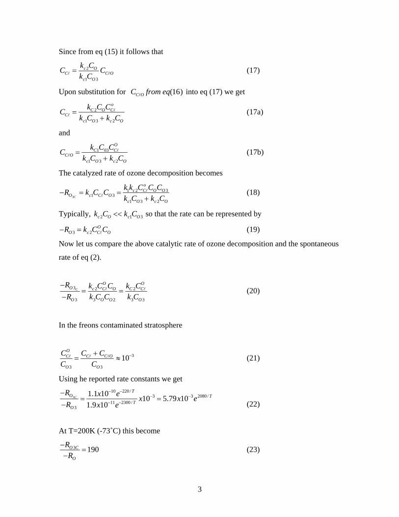
In the freons contaminated stratosphere
CClO
CO3
=CCl + CClO
CO3
≈10−3 (21)
Using he reported rate constants we get
−RO3C
−RO 3
=1.1x10⁻¹⁰e−220 / T
1.9x10⁻¹¹e−2300 / T x10−3 = 5.79x10⁻³e2080 / T
(22)
At T=200K (-73˚C) this become
−RO 3C
−RO
=190 (23)

4
Thus the presence of CFCs accelerates ozone decomposition almost 200 times! For full
explanation of the dynamics of the ozone hole above Antarctica read the Rowland and
Molina’s paper. Now you have the tools to understand it.
Remember that other components such as oxides of nitrogen contribute significantly to
ozone dynamics.

REACTION MECHANISMS AND
EVALUATION OF RATE FORMS
(CHE 505)
M.P. Dudukovic
Chemical Reaction Engineering Laboratory
(CREL),
Washington University, St. Louis, MO

ChE 505 – Chapter 5N Updated 01/31/05
5. REACTION MECHANISMS AND EVALUATION OF RATE FORMS We have already seen that single reactions, in general, do not occur in one step; but that it is a particular sequence of elementary reactions (reaction mechanism) that leads to the overall reaction. The knowledge of the reaction mechanism is extremely desirable since then the overall rate can be determined from first principles of the law of mass action which applies to every elementary step in the sequence. If such an attempt results in too complex algebraic expressions, at least experiments can be designed to test whether certain steps of the mechanism are rate limiting, which helps in finding a simplified rate form. Knowledge of the expected rate form helps in designing the right experiments for rate determination. Reaction Mechanism - this sequence of elementary events represents the detailed pathway of transformation of the reactants through highly reactive intermediates (active centers) to final products. Based on the structure of this sequence we can draw a more appropriate distinction between catalytic and noncatalytic processes. An open sequence is one in which an active center is not reproduced in other steps of the sequence. The reaction is noncatalytic. A closed sequence is one in which an active center is reproduced so that a cyclic pattern repeats itself, and a large number of molecules of products can be made from only one active center. Reaction is catalytic. Let us consider some examples: Mechanism 1: active center −+ +⇔ ClRRCl +R ; open sequence; noncatalytic RFFR ⇔+ −+
------------------------- Overall stoichiometry: −− +⇔+ ClRFFRCl Mechanism 2: active center ES*; closed sequence; *ESSE ⇔+ catalytic PEES +⇔ ------------------------ Overall stoichiometry: S = P E This second mechanism above is the Michaelis-Menten mechanism for enzyme catalyzed reactions such as isomerization of glucose, etc. We should be particularly careful to spot a closed sequence loop within a larger mechanistic path. For example, a typical chain propagation reaction follows Mechanism 3 below:
1

ChE 505 – Chapter 5N Updated 01/31/05
5*2
4*1
*2
1*1
3*1
*2
*221
*1
*11
2
2
2
MR
MRR
MR
MRR
RMMRRM
→
→+
→
+→
+→+
→
Steps 2 and 3 of the above mechanism form a closed (catalytic) sequence in which the active centers (intermediates, radicals) are repeatedly regenerated. #
2*1 RandR
Basic Rule: Whenever a mechanism is hypothesized for a single reaction consisting of N elementary steps the weighted sum of the N steps (i.e. the sum of all steps each of them multiplied by an integer 1, 2, 3 etc.) must result in the overall stoichiometry for the reaction under consideration. If it does not, the mechanism is not consistent with stoichiometry and should be discarded. The above Basic Rule has to be applied judiciously. It is certainly true for an open sequence mechanism. As a matter of fact, it can be used then to discard the steps that are incompatible. However, in mechanisms containing a closed sequence it is the steps of the closed sequence that must lead to the overall stoichiometry. In our mechanism 3 above, the stoichiometry is 321 MMM += . The fact that termination of active centers may lead to or is immaterial since those would be present in an infinitesimal amount and would not affect the mass balance of the single reaction under consideration
i.e.
*2R 4M 5M
,111
321 nnn ∆=
∆=
−∆ .
However, the "impurities" (e.g., and ) resulting from such a mechanism may be important from an environmental standpoint and we should strive to understand what they are and in what amounts they could form.
4M 5M
Finding the multipliers (stoichiometric numbers), by which certain steps of the mechanism have to be multiplied in order to lead to the overall stoichiometry upon summation, is a trivial matter for relatively simple mechanisms consisting of two to three steps. For example, if a single reaction stoichiometry is given by 2A = R and the mechanism is Mechanistic Step Stoichiometry of the Step Stoichiometric Number 1. AAAA +⇔+ * A = A* 2 2. RAA ⇔+ ** 2A* = R 1 Overall Stoichiometry: 2A = R it is clear that the first step should be repeated twice (stoichiometric number ) in order to get the overall stoichiometry.
21 =v
For lengthy complex mechanisms simple inspection may not be the best way to proceed. If the reaction stoichiometry is given in such a way that all stoichiometric coefficients are integers (which can always
2

ChE 505 – Chapter 5N Updated 01/31/05
be done by multiplying through with an appropriate number) then the reaction stoichiometry may be written as:
(1) ∑=
=S
jjj Av
1
0
If the mechanism consists of N steps, and the stoichiometric coefficient of species j in step i is , then the steps of the mechanism can be presented by a set of linear equations:
ijv
(2) NiAvS
jjij ...3,2,1for0
1
1==∑
=
In order for the mechanism to be consistent with stoichiometry we must be able to find a set of stoichiometric numbers (multipliers) not all zeroNivi ,....2,1= from the following set of linear equations:
(3) ∑=
==N
ijij
i Sjvvv1
1...3,2,1for
where is the total number of species including active intermediates, i.e.1S , where I is the total number of active intermediates. Naturally the overall stoichiometric coefficients for active
intermediates must all be zero.
ISS +=1
jv11 ,1.....,3,2,1 SSSSSj −+++=
Example:
Mechanism: Stoichiometry of each step: AAAA +⇔+ * *AA = RAA ⇔+ ** RA =*2 Overall Stoichiometry: RA =2
A: 201 −=+− v 21 =v R: 10 2 =+ v 12 =v I: 02 21 =− vv
Thus we have a set of equations 1S ( )3121 =+=+= ISS with N unknowns ( )iv ( 2)=N . The nonzero solution for exists if the matrix of has rank N. If that is the case select N equations and
solve for .
iv ijviv
In the above simple example we have one intermediate species (A*) so that I = 1 and we have two stable species (A and R) so that S = 2 and hence S1 = S + I = 3. The mechanism consists of two steps so that N = 2 and we need to determine the two stoichiometric numbers and by which step 1 and step 2, respectively, should be multiplied to arrive at the overall stoichiometry. If we number A, R and A* as species 1, 2, and 3, in that order, equation (3) can be written in the following matrix form:
1v 2v
3

ChE 505 – Chapter 5N Updated 01/31/05
( ) ⎟⎟⎠
⎞⎜⎜⎝
⎛−=⎟⎟
⎠
⎞⎜⎜⎝
⎛−
−12
21010121 νν (3a)
The matrix of stoichiometric coefficient ( )ijν is:
⎟⎟⎠
⎞⎜⎜⎝
⎛−
−210
101
and the nonzero solution for the ( )21 νν vector is guaranteed if that matrix has rank 2 which it clearly does. The matrix multiplication in eq (3a) results in 3 rows that are presented above which generate the solution for and . See any text on linear algebra or matrices for details if you encounter a problem of this nature. A good reference for chemical engineers is Amundson N.R., "Mathematical Methods in Chemical Engineering-Matrices and Their Applications", Prentice Hall, 1966.
1ν 2ν
When a consistent mechanism is proposed, the overall rate of reaction can be derived based on one of the following two assumptions: 1. Pseudo-steady state assumption (PSSA), also called Quasi-steady state assumption (QSSA) 2. Rate limiting step assumption (RLSA) 5.1. PSEUDO-STEADY STATE ASSUMPTION (PSSA) Since the intermediates (active centers) which may be of various nature, (e.g., free radicals, ions, unstable molecules etc.) appear only in the mechanism but not in the overall stoichiometry for the reaction it can be safely assumed that their concentration is at all times small. If this was not so, then they would be detectable and would appear in the overall stoichiometry since a substantial portion of the reactants would be in that form at some point in time. Now, reasoning leads us to conclude that then the net rate of formation of these active intermediates must also always be small. If this was not true, and if at some point in time the net rate of formation was high, then the quantity of this intermediate would have to rise and we have already concluded that this cannot happen. Thus, the net rate of formation of all the active intermediates involved in the mechanism, but not appearing in the overall stoichiometry for the reaction, must be very small. This is the basic hypothesis of the PSSA: The net rates of formation of all active intermediates are negligibly small and hence are approximately zero.
This requirement for a mechanism of N steps including S stable species that appear in overall reaction stoichiometry and I intermediates can be formally written as: ISS +=1
(4) ∑=
+===N
ijiij SSjRrv
1
1,...1for0
4

ChE 505 – Chapter 5N Updated 01/31/05
From these I linear expressions we can evaluate the I concentrations of the intermediates in terms of the rate constants and the S concentrations of stable species. Substituting these intermediate concentrations into the expression for the rate of a desired component j
(5) Sj
rvRN
iiijj
,....2,11
=
= ∑=
we obtain the required rate form for that component. Thus, the procedure for applying the PSSA to a single reaction can be outlined as follows: 1. Write down the hypothesized mechanism and make sure that it is consistent with stoichiometry. 2. Count all the active intermediates. 3. Set up the net rate of formation for every active intermediate. Remember, since the steps in the
mechanism are elementary, law of mass action applies in setting up rates of each step. Make sure to include the contribution of every step in which a particular intermediate appears to its net rate of formation.
4. Set all the net rates of active intermediates to be zero and evaluate from the resulting set of
equations the concentrations of all active intermediates. 5. Set up the expression for the rate of reaction using a component which appears in the fewest steps
of the mechanism (in order to cut down on the amount of algebra). Eliminate all the concentrations of active intermediates that appear in this rate form using the expressions evaluated in step 4. Simplify the resulting expression as much as possible.
6. If you need the rate of reaction for another component simply use the rate form evaluated in step 5
and the relationship between the rates of various components and their stoichiometric coefficients. 7. If there is solid theoretical or experimental information which indicates that certain terms in the
rate form obtained in step 5 or 6 may be small in comparison to some other ones simplify the rate form accordingly.
8. Check the obtained rate form against experimental data for the rate. 9. Remember that even if the derived rate form agrees with experimental data that still does not prove
the correctness of the proposed mechanism. However, your rate form may be useful especially if the reaction will be conducted under conditions similar to those under which experimental data confirming the rate form were obtained.
Let us apply this to an example. Consider the decomposition of ozone. We want to know its rate. The overall stoichiometry is (6) 23 32 OO = 1. The proposed mechanism consists of 2 steps:
5

ChE 505 – Chapter 5N Updated 01/31/05
*
23
1
1OOO
fk
bk+⎯⎯ →⎯
⎯⎯ ⎯← (7a)
223
* 2 OOOO k +⎯→⎯+ (7b) The mechanism is obviously consistent with the overall stoichiometry, the stoichiometric number
of both steps being one. We have already assumed that the last step is irreversible since it is highly unlikely that two
oxygen molecules would spontaneously "collide" to produce an active oxygen atom and ozone. 2. Counting the active intermediates we find one, namely, . *O 3. The net rate of formation of is: *O
03**23* 211 =−−= OOOObOfO
CCkCCkCkR (8) 4. According to PSSA the above rate must be zero. From the above equation we get
3*
2 3
1
1 2
f OO
b O O
k CC
k C k C=
+ (9)
5. Since both and appear in both steps of the mechanism we can set up the rate of
disappearance of ozone directly 2O 3O
3*2*33 211 OOOObOfO CCkCCkCkR +−=− (10) Substituting the expression for , and finding the common denominator, leads to: *O
C
3 2 3 3 2 3
3
2 3
3
3
2 3
2 21 1 1 2 1 1 1 2
1 2
21 2
1 2
2
f b O O f O f b O O f OO
b O O
f OO
b O O
k k C C k k C k k C C k k CR
k C k C
k k CR
k C k C
+ − +− =
+
− =+
(11)
This is a complete rate expression based on the hypothesized mechanism.
7. Concentration of ozone is orders of magnitude smaller than the concentration of oxygen. It also
appears that the second step in the mechanism is slow. Thus, when the rate simplifies to:
32 21 OOb CkCk >>
2
3
3
2
1
212
O
O
b
fO C
Ck
kkR ≈− (12)
6

ChE 505 – Chapter 5N Updated 01/31/05
8. The experimentally found rate under these conditions of low is . Agreement seems to exist between the proposed mechanism and data.
3O 12233
−= OOO CCkR
Consider another example. The overall reaction stoichiometry is given as: A + B = R (13) and the experimentally determined rate is (14) 2
AA CkR =− It is desired to determine whether the mechanism outlined below is consistent with the observed rate. 1. (15a) IAA k⎯→⎯+ 1
(15b) ARBI k +⎯→⎯+ 2
2. The mechanism is obviously consistent with the overall stoichiometry since a straight forward
addition of steps leads to it. The number of intermediates is one, I. 3. The net rate of formation of the intermediate is:
0 (16) 22
1 =−= BIAI CCkCkR 4. And according to PSSA is equal to zero. The concentration of I is then
B
AI Ck
CkC2
21= (17)
5. Since A appears in both steps of the mechanism and R only in one, set up the rate of formation of R for convenience
(18) BIR CCkR 2=
Eliminating we get IC
(19) 21 AR CkR =
6. From stoichiometry
2111 A
RA CkRR==
− (20)
7. The rate agrees with the experimentally determined one. (Compare eq. (20) and (14)). The
mechanism may be right.
7

ChE 505 – Chapter 5N Updated 01/31/05
NOTE: In writing the net rate of formation of , in step 3 we used the equivalent rate and thus based the rate constant on I. If we were to write the rate of disappearance of A,
IRI ,
1k (21) BIAA CCkCkR 2
212 −=−
notice that the first term has to be multiplied by the stoichiometric coefficient of A in the 1st step, which is two, since the rate of disappearance of A in the 1st step is twice the rate of appearance of I in that step. If we followed a different convention we would have based on the left hand side from where the arrow originates i.e.
1k we would have based it on a component A. In that case a factor1/2 would have
appeared with k in step 3 and there would be no 2 but 1 in front of in the expression for 1 1k AR− . This seemingly trivial point often causes a lot of errors and grief. Just notice that if we forgot the proper stoichiometric relationship, and the expression for AR− in eq. (21) did not have a 2 but , while was as given, they would be identically equal to each other and thus asserting would be asserting that , which is absurd since
1k 1k IR0=IR
0=− AR RA RR =− which is a respectable expression. This demonstrates the importance of not forgetting the stoichiometric coefficients in setting up rates. At the end it should be mentioned that the PSSA fortunately does not only rest on the verbal arguments presented at the beginning of this section (can you find any fault with this?) but has solid mathematical foundations originating in the theory of singular perturbations. This will be illustrated in an Appendix since the same theory is applicable to may other situations. The application of PSSA to multiple reactions is a straightforward extension of the above procedure. 5.2 RATE LIMITING STEP ASSUMPTION (RLSA) This approach is less general than the previous one, in the sense that we must know more about the mechanism than just its form in order to apply it. The rate expression obtained from RLSA represents thus a limiting case of the one that could be obtained using PSSA. The basic hypothesis of the RLSA is as follows: 1. One step in the mechanism is much slower than the others and thus that rate limiting step
determines the overall rate. 2. With respect to the rate limiting step all other steps may be presumed in equilibrium. This is best explained based on an example. Consider a reaction 2A + B = R. Suppose that we want to find its rate form based on the mechanism shown below. In addition, it is known that the 1st step is the slowest. If we then depict the magnitude of the forward and reverse rates for each step with , and the magnitude of the net forward rate by a solid arrow, and if we keep in mind that the net rate must be of the same magnitude in all the steps (which is required by PSSA) because otherwise the active intermediates would accumulate someplace, we get the picture presented to the right of the hypothesized mechanism below. 1. *1
1AA
fk
bk
⎯⎯ ⎯←⎯⎯ →⎯
8

ChE 505 – Chapter 5N Updated 01/31/05
2. ** 2
2ABBA
fk
bk
⎯⎯ ⎯←⎯⎯ →⎯+
3. RAAB
fk
bk
⎯⎯ →⎯⎯⎯ ⎯←+3
3
**
Clearly the magnitude (length)of the arrows indicating forward and reverse rates isthe smallest in step 1, this step is the slowest and limits the rate. At the same time the magnitude of the net rate forward is almost 1/2 of the total rate forward in step 1 and that step clearly is not in equilibrium while the magnitude of the net rate forward ( ) in comparison to the total rate forward ( ) and total reverse rate (←) in steps 2 and 3 is negligible. Thus, in these two steps rates forward and backward are approximately equal, and in comparison to step 1 these two steps have achieved equilibrium. Thus, the procedure for applying the RLSA to a single reaction can be outlined as follows: 1. Write down the hypothesized mechanism and make sure that it is consistent with stoichiometry. 2. Determine which is the rate determining step. This should be done based on experimental
information. Often various steps are tried as rate limiting due to the lack of information in order to see whether the mechanism may yield at all a rate form compatible with the one found experimentally.
3. Set up the net rates of all the steps, other than the rate limiting one, to be zero, i.e. set up
equilibrium expressions for all other steps. 4. Set up the rate form based on the law of mass action for the rate determining step, and eliminate all
concentrations of intermediates using the expressions evaluated in step 3. 5. Using the stoichiometric number of the rate determining step relate its rate to the desired rate of a
particular component. 6. Check the obtained rate form against the experimentally determined rate. 7. Remember that the agreement or disagreement between the derived and experimental rate form
does not prove or disprove, respectively, the validity of the hypothesized mechanism and of the postulated rate limiting step. If the two rate forms disagree try another rate limiting step and go to step 3. If the two rate forms agree use the rate form with caution.
The greatest limitation of the rate forms based on RLSA is that they are much less general than those developed from PSSA and they do not test the mechanism in its entirety. The rate forms based on RLSA may be valid only in narrow regions of system variables (e.g., T, concentrations) since with the change in variables (i.e. concentrations, T) the rate limiting step may switch from one step in the mechanism to another. Clearly, the magnitude of our arrows representing the rates depends on concentration levels, temperature, pressure etc. and may change rapidly as conditions change. An example in the shift of the rate limiting step is the previously covered Lindemann's-Christensen mechanism for unimolecular reactions. Suppose that we want to evaluate the rate of formation of R for the reaction given above and under the assumptions made.
9

ChE 505 – Chapter 5N Updated 01/31/05
1. We first test the compatibility of the proposed mechanism with stoichiometry. By inspection we find:
*22 AA = 2 (22a) 1 =v
** ABBA =+ 1 (22b) 2 =vRAAB =+* 1 (22c) 3 =v
RBA =+2 2. Step 1 is rate limiting (given) 3. Set up equilibrium expressions for step 2 and 3
BA
AB
b
fC CC
Ckk
K*
*
22
2 == (23a)
BAC
R
AAB
R
b
fC CCK
CCC
Ckk
K 23
3
2**
3=== (23b)
4. Set up the rate for the rate limiting step
(24) *1 AbAf CkCkr −=l
Using eq. (23b) and eliminating we get *A
C
BCC
RA CKK
CC32
* =
21
211
1
32 B
R
CC
bAf C
CKK
kCkr −=l (24a)
5. The stoichiometric number of the rate limiting step is as per (eq. 22a). Thus, since 2== sv l
llr
vvR R
R =
21
2111
32222
1
B
R
CC
bA
fR C
CKK
kC
krR −== l (25)
6. Information not available.
Now suppose that in the same mechanism step 2 was rate limiting (i.e. arrows for the rate of step 2 now being much shorter than those in step 1 and 3). We can quickly write the equilibrium relationships for step 1 and 3:
10

ChE 505 – Chapter 5N Updated 01/31/05
b
f
A
AC k
kCCK
1
11
*
== (26a)
**3
33
AAB
R
b
fC CC
Ckk
K == (26b)
and from these obtain the concentrations of the intermediates (27a) ACA CKC 1
* =
ACC
RAB CKK
CC31
* = (27b)
The rate for the rate limiting step (step 2) is: (28) ** 22 ABbBAf CkCCkr −=l
ACC
RbBACCf
A
R
CC
bBACfe CKK
CkCCKKkCC
KKk
CCKkr
31
22
32
12
31
212
−=−= (28a)
since (29) eR rR = 1=lv
Clearly this is an entirely different rate form than obtained previously based on step 1 being rate limiting. NOTA BENE 1: It would be quite tedious to find the rate form for the above mechanism based on PSSA since when the net rates of formation of intermediates are set to zero we get nonlinear equations due to the product resulting from the rate forward in step 3. Try it anyway for an exercise. **
AAB CC NOTA BENE 2: If the first step ( )21 =v was rate limiting our rate form is given by
21
21
32
11
22 B
R
CC
bA
fR C
CKK
kC
kR −= (25)
21
21
B
RbAf C
CkCk −=
At equilibrium so that 0=RR
21
21
321
1
BA
RCC
b
f
b
f
CCCKK
kk
kk
== (30)
Recall that 11
1C
b
f Kkk
= (31a)
11

ChE 505 – Chapter 5N Updated 01/31/05
and that for the reaction 2A + B = R the equilibrium (concentration units) constant is given by CK
BA
RC CC
CK 2= (31b)
Substituting eqs. (31a) and (31b) into eq. (30) we get
21321 CCCC
b
f KKKKkk
== (32)
Recall that sCP
Cb
f KKkk 1
== where s is the stoichiometric number of the rate determining step.
Here . Hence, 21 == vs (33) 32
21 CCCC KKKK =
If the 2nd step ( )12 =v is rate limiting the rate form is given by eq. (28a)
A
R
CC
bBACfR C
CKK
kCCKkR
31
212 −= (28a)
A
RbBAf CCkCCk −=
so that at equilibrium 0=RR
'2 C
BA
R
b
f KCC
Ckk
== (33)
and 322
132
12
2CCCCC
b
fC KKKKK
kk
K == (33)
Let us go back to the reaction of decomposition of ozone 23 3020 = . The mechanism was given before and let us assume that the 2nd step is rate limiting. Then
3
2
1
11
*
O
OO
b
fC C
CCkk
K == (34a)
2
31*
O
OCO C
CKC = (34b)
12

ChE 505 – Chapter 5N Updated 01/31/05
2
23
1232 *
O
OCOO C
CKkCCkr ==l (35)
Now 2but1
3== Ovv l
Thus, 2
23
1
21
2
23
123
22
O
O
b
f
O
OCO C
Ck
KkCC
KkR ==− (36)
Notice that this is the rate form obtained when using PSSA after certain additional assumptions were made. The rate form generated by the use of PSSA without additional assumptions is much more general. The above expression is its limiting case. For multiple reactions, rate forms can be obtained by RLSA by the straightforward extension of the above rules. 5.3 HALF LIFE AND CHARACTERISTIC REACTION TIME Based on either PSSA or RLSA we are usually able to derive a rate form for a particular reaction. Often n-th order rate form is obtained , say for reactant j: ( ) n
jj kCR =− (37)
Then the characteristic reaction time is defined as 1
1−= n
joR kC
τ and it is the time that it would take
in a close system (batch) for the concentration to decay to of its original value . jC 1−e joC
The balance for reactant j in a closed system is jj R
dtdC
−= . So when the reaction is not n-th order the
characteristic reaction time can be defined as jo
joR R
C=τ where the rate is evaluated at initial
conditions.
joR
Half-life is the time needed for the reactant (species) concentration to be reduced to half of its original value in a closed system. Integration of the species balance yields
∫∫∫∫ ====1
21
1
21
2
21
21
Rcd
Rcd
RC
RdC
dtt Rjo
joC
C j
jt
o
jo
jo
τ (38)
where joj CCc = and joj RRR = . The integration is performed by substituting into the above expression all concentrations in terms of using the stoichiometric relations. For an n-th order reaction we get
jC
13

ChE 505 – Chapter 5N Updated 01/31/05
( ) ( ) R
n
njo
n
nCnkt τ
112
112 1
1
1
21 −−
=−
−=
−
−
−
(39)
For a first order process
2ln2ln21 Rk
t τ== (39a)
5.4 COMPARTMENTAL MODELING OF SINGLE PHASE SYSTEMS We should note that in developing the rate forms based on mechanisms we have so far assumed that we deal with a system of constant mass consisting of fixed amounts of various atomic species. These atomic species are constituents of chemical species (components) that participate in elementary chemical reactions taking place in the system. These chemical species are either stable, and present in measurable concentrations (e.g. reactants and products), or are active intermediates present in much smaller concentrations. The volume of the system (i.e. of the invisible envelope that engulfs our constant mass) is small enough that molecules are free to interact by molecular motion so that concentration or temperature gradients can never develop in the system. Hence, the system is well mixed. Moreover, the system is closed since no exchange of mass occurs across system’s boundaries. We extend this approach now to modeling of isothermal, single phase systems or arbitrary volume. We assume that the volume of the system is perfectly mixed at all times so that there never are any spatial composition gradients in the system. We can apply then the basic conservation law to quantities of the system that are conserved (e.g. mass, species mass, energy etc.) that states: ( ) ( ) ( ) ( )generation of Rateoutput of Rateinput of Rateonaccumulati of Rate +−= (40) Such a well mixed system, to which we apply equation (40) often is called a compartment - hence, the name compartmental modeling. We can have closed systems (no exchange of mass across system’s boundary) and open systems (that exchange mass with the surroundings). Here we focus only on single phase systems and we start by developing the governing equation for a closed system. A sketch of a closed system is shown below:
( )tc t t c c t
MV
j
jij
=
==
At time0 At time
MASS - VOLUME -
OF SYSTEM
- Total mass of the system ( ) constkgM =- Total volume of the system ( )3mV may vary in time
- Vnm
jmolc jj =⎟⎠⎞
⎜⎝⎛
3 molar concentration of species j in the system at time t
14

ChE 505 – Chapter 5N Updated 01/31/05
- ⎟⎠⎞
⎜⎝⎛
smmolR j 3 = reaction rate of j
For a well mixed closed system the species mass balance for species j can be written as:
d VCj( )
dt= VRj ; t = 0, Cj = Cjo (41)
where
Cjmol j
L⎛ ⎝
⎞ ⎠ = molar concentration of j at time t
V(L) = volume of the system t (s) = time
Rjmol j
L s⎛ ⎝ ⎜ ⎞
⎠ = reaction rate of production of species j (if j is a reactant Rj < 0)
Cjomol j
L⎛ ⎝
⎞ ⎠ = initial concentration of species j
Note: units of time instead of seconds could be minutes, hours or days; volume could be measured in m3, etc. If the volume of the system is constant V = const, eq (41) is reduced to:
dCj
dt= Rj ; t = 0, Cj = Cjo (41a)
If we have R reactions occurring in the system, then their stoichiometry is given by:
υijj =1
s
∑ Aj = 0 ; i = 1,2,...R (42)
here υij = stoichiometric coefficient of species j in reaction i (recall υij > 0 products, υij < 0 reactants) and S = total number of stable species in the system. Often, in chemical as well as in environmental systems such as encountered in air or water pollution, the set of R reactions is extended to include all active intermediate species (their total number is ) that are linked among themselves and with stable species via a large set of R' elementary reactions based on the proposed mechanism. (Note R’ > R).
'S
This augmented set of R' elementary reactions arising from the mechanism can be written as
υ ijm
j =1
S +S '
∑ A j = 0 ; i = 1,2,... 'R (43)
where υij
m is the stoichiometric coefficient chemical species of j in the mechanistic step i.
15

ChE 505 – Chapter 5N Updated 01/31/05
There are two ways now to proceed. a) An exact solution can be obtained by solving equation (41a) for all the S + S' species, stable as well as active intermediates, i.e for j = 1,2,3...S,S+1, S+2...S+S'. This can be stated as:
dCj
dt= Rj = υij
m
i=1
R'
∑ ri ; t = 0, Cj = Cjo (44)
for j = 1,2,...S, S + 1... (S' + S) where ri is the reaction rate of the elementary reaction i in the proposed mechanism for which the rate constant is evaluated from transition state theory (TST) or by other appropriate means. For each of the stable compounds (j = 1,2...S) the initial concentration, Cjo, is known, for all active intermediates (j = S + 1, S + 2...S + S') the initial concentration is zero, Cjo = 0. This (eq (44)) results in a stiff system of differential equations which must be solved by an appropriate computer package. Numerical solution is almost always required. The stiffness (vastly different eigenvalues) is caused by a wide range of time constants. The results can be displayed for active intermediates as well as stable compounds as functions of time. b) An approximate solution can be obtained by using PSSA. For all active intermediates we set
for j = S + 1, S + 2,...S + S' (45) Rj = υijm
i =1
R'
∑ rj = 0
From the resulting S' equations (often nonlinear) we evaluate the S' concentrations of active intermediates which then can be substituted into the rate forms for stable species. S differential equations need to be solved now (instead S+S’):
dCj
dt= Rj = υijri
o
i=1
R
∑ ; t = 0, Cj = Cjo (46)
only for the S stable species (j = 1,2,3...S). The reaction rate for reaction i among stable species, r , is now obtained from the mechanism by applying PSSA and eliminating the concentrations of active intermediates. These expressions for r are not rates of elementary reactions necessarily, and can be of rather complex form. Upon solution of equation (46) for the concentrations of the stable species these can be displayed as function of time. The concentrations of the active intermediates can then be calculated from the solution of equation (45) and are constant in time. Nota bene
io
io
: More complex dynamic behavior with limit cycles, etc., can also be encountered. Concentrations of active intermediates are always small. 2. Open System A sketch of the open system is shown below:
inQ
joC
outQ
jC V
M VOLUME
MASSOR SYSTEM
16

ChE 505 – Chapter 5N Updated 01/31/05
- ( )smQin
3 = volumetric flow rate in - ( )smQout
3 - volumetric flow rate out - for all j. Outlet of perfectly mixed system is representative of system’s content. joutj CC ≡ In the open system all the species are brought in and out across the system’s boundary. We will assume here that this happens by convection only, and that the volumetric flow rate in and out is the same,
( ) outin QQsLQ == . The species balance which is based on the basic conservation equation (40) can be written as:
VdCj
dt= RjV + Q Cjin
− Cj( ); t = 0, Cj = Cjo (47)
where Cjin
mol jL
⎛ ⎝
⎞ ⎠ is the concentration of species j in the incoming (feed) flow. Due to the assumption
of perfect mixing the concentration of j in the exit flow is the same as the concentration Cj of j at that time in the system. The rate Rj is given as before. Again one can go for the exact solution by applying eq (47) to all species, j = 1, 2, 3...S + S'. Or one can attempt a PSSA solution by setting Rj = 0 for j = S + 1, S + 2,...S + S' and by solving eq (47) for j = 1, 2...S for the stable species only.
An open system can reach steady state when dCj
dt= 0 and then
(−Rj)V = Q Cjin
− Cj( ) (47a) In complex reaction networks true steady state may never be reached as cycles set in. We can apply now the compartmental single phase model to gaseous systems contained in a vessel, in a room, urban atmosphere or in the whole atmosphere. The underlying assumption is then that in the volume we have chosen mixing is perfect so that no composition spatial gradients occur at any time. Otherwise we must divide the system into a number of compartments and describe the flows between them. Let us consider some gas phase atmospheric reactions next. 5.5 GAS-PHASE ATMOSPHERIC REACTIONS Atmosphere is an oxidizing environment with abundance of solar energy (during day time hours) so that the pollutants are continuously brought to a higher and higher oxidation state. Hydrocarbons are reacted to aldehydes, then acids, then CO2. Sulfur containing compounds are oxidized to SO2 and ultimately to H2SO4. Ammonia and other nitrogen containing species are oxidized to NO, then NO2 and HNO3. 5.5.1 Atmospheric Photochemical Reactions These are initiated by absorption of a photon by an atom, molecule, radical or ion. *kA h Aν+ ⎯⎯→
17

ChE 505 – Chapter 5N Updated 01/31/05
The excited activated molecule (radical), A * , can participate in four different reaction types (1) 1*
1dissociation kA B⎯⎯→ + 2B
h (2) 2*
1direct reaction kA B C+ ⎯⎯→ 3*fluorescence kA A ν⎯⎯→ + (3) (4) 4*collisional deactivation kA M A M+ ⎯⎯→ + Reactions (1) and (2) lead to chemical change while (3) and (4) return the molecule to its ground state. The quantum yield, iφ , of a process (i = 1 to 4) is defined as the ratio of the number of radicals A * reacting by that process to the number of photons absorbed. The active intermediate A * is short lived so that PSSA applies
[ ] [ ] [ ]* * * ** 1 2 3 40 AR k A k A k A B k A k A M⎡ ⎤ ⎡ ⎤ ⎡ ⎤ ⎡ ⎤= = − − − −⎣ ⎦ ⎣ ⎦ ⎣ ⎦ ⎣ ⎦
[ ][ ] [ ]
*
1 2 3 4
k AA
k k B k k M⎡ ⎤ =⎣ ⎦ + + +
The rate of formation of [A *] by absorption of light is k [ A ] where k is the specific absorption rate (k first order rate constant independent of [A ] ). Using the quantum yield definition for the above four processes we can write [ ]
1
*1 1BR k A k Aφ⎡ ⎤= =⎣ ⎦
[ ] [ ]1
*2 2CR k A B k Aφ⎡ ⎤= =⎣ ⎦
[ ]*3 3AR k A k Aφ⎡ ⎤= =⎣ ⎦
[ ] [ ]*4 4AR k A M k Aφ⎡ ⎤= =⎣ ⎦
So that . 4
11i
iφ
=
=∑ The solar flux, or actinic irradiance, F , (photons/cm2s) is the radiation intensity striking a unit area of surface per unit time. ( )dF I dλ λ= where ( )I dλ λ = actinic irradiance in the wave length range ( to dλ λ λ+ ) so that the actinic
irradiance density ( )I λ is in (photons/cm3s). We are most interested in dissociation reactions for which the first order rate constant is given by
18

ChE 505 – Chapter 5N Updated 01/31/05
( ) ( ) ( )2
1
1 , ,A Ak T T Iλ
λ
dσ λ φ λ λ= ∫ λ
)
where = absorption cross-section of A at wave length ( ,A Tσ λ λ and temperature T
= the quantum yield or probability that molecule A decomposes on absorbing ( ,A Tφ λ ) radiation of wave length λ at temperature T. The integral is usually approximated by summation. In the troposphere the wave lengths of interest are 280 nm < λ < 730 nm. Stratosphere O2 and O3 block out most small wave lengths λ < 280 nm. No chemistry occurs at λ > 730 nm. Absorption cross-sections and quantum yields are measured in laboratory. (Examples are shown in Figures 1 and 2). The major variable is the intensity change that occurs as a function of time of day, latitude, time of year and state of the atmosphere (e.g. humidity, cloudiness, particulates, etc.). Solar flux as a function of λ is shown in Figure 3. In the US maximum noontime, intensity in summer months is about 2 x 10¹⁶ (photons/cm2s) in the 300-400 nm range and is close to this value for 4-6 hours. In winter, 0.7 x 10¹⁶ to 1.5 x 10¹⁶ (photons/cm2s) are typical values depending on the latitude. Major photo dissociating species in the lower atmosphere are summarized in Table 1. FIGURE 1: Absorption cross section for O3 and NO2 in the uv and visible regions of the
spectrum (Luther and Gelinas, 1976)
FIGURE 2: Experimental quantum yield data for the production of atomic oxygen (O)
from the photolysis of NO2 as a function of wavelength. The dashed line represents the quantum yields suggested by Demerjian et al. 91980).
19

ChE 505 – Chapter 5N Updated 01/31/05
20

ChE 505 – Chapter 5N Updated 01/31/05
FIGURE 3: Direct solar flux at 0 and 15 km as a function of wavelength (National Center for Atmospheric Research, 1982).
21

ChE 505 – Chapter 5N Updated 01/31/05
TABLE 1: Major photodissociating species in the lower atmosphere.
22

ChE 505 – Chapter 5N Updated 01/31/05
TABLE 1CONTINUED:
From J. Seinfeld. Air Pollution
23

ChE 505 – Chapter 5N Updated 01/31/05
5.5.2 Ozone Formation - NOx Route When nitrogen oxides (NO or NO2 ) are present in sunlight, ozone formation occurs as the result of NO2 photolysis. The mechanism is as follows: (1) 1
2kNO h NO Oν+ ⎯⎯→ +
(2) 22
kO O M O M+ + ⎯⎯→ +3
2 2 (3) 33
kO NO NO O+ ⎯⎯→ + This is an entirely closed cycle in which the energy is ultimately absorbed by the third body, M , and no overall change occurs. However, the dynamics of the system are of interest in determining if one starts with a certain concentration of [ ]o
NO and [ ]2 oNO what would the peak concentration of ozone [ ]
max3O be. Clearly PSSA implies [ ] [ ][ ][ ]1 2 2 2 0OR k NO k O M O= − =
[ ] [ ][ ][ ]1 2
2 2
k NOO
k O M=
Since [O 2 ], [M ] are large and approximately constant we see that [O ] adjusts itself rapidly by following [N O 2 ]. A species balance for ozone in a closed system (i.e system of constant volume with no exchange with surroundings) yields
[ ] [ ][ ][ ] [ ][ ]3
32 2 3 3O
d OR k O O M k O NO
dt= = −
Upon substitution of [O ] in the above we get
[ ] [ ] [ ][3
31 2 3 3O
d O ]R k NO k O NOdt
= = −
Similarly making a balance on N O and N O 2 we get
[ ] [ ] [ ][1 2 3 3NO
d NO ]R k NO k O NOdt
= = −
[ ] [ ] [ ][2
21 2 3 3NO
d NO ]R k NO k O NOdt
= = − +
From the above it is evident that
[ ] [ ]{ }3 0d O NOdt
− =
24

ChE 505 – Chapter 5N Updated 01/31/05
so that [ ] [ ] [ ] [ ]3 3 o
O O NO NO− = −o
It is also evident that
[ ] [ ]{ 2 0d NO NOdt
+ } =
so that [ ] [ ] [ ] [ ]2o o
NO NO NO NO− = − 2 Using these relations we eliminate both concentrations of N O and N O 2 in terms of the concentration of ozone and of the initial concentrations indicated by subscript o [ ] [ ] [ ] [ ]3o o
NO NO O O= − + 3
[ ] [ ] [ ] [ ]2 2 3o oNO NO O O= + − 3
which yields the following rate of change of ozone concentration for any starting mixture
[ ] [ ] [ ] [ ]{ } [ ] [ ] [ ] [ ](31 2 3 3 3 3 3 3o o o o
d Ok NO O O k O NO O O
dt= + − − − + )
At [ ] [ ]3 30
ot O= = O
We are at the moment only interested in the maximum ozone concentration which occurs at the
pseudostationary state i.e when [ ]3 0.d O
dt= We can also look at it as the PSSA solution to the problem
if we assume O3 also to be an active intermediate. This is justified since its concentration is always much smaller than that of oxides of nitrogen. Now we get:
[ ] [ ][ ]
[ ] [ ] [ ][ ] [ ] [ ]( )
1 2 3 31 23
3 3 3
( )o o
o o
k NO O Ok NOO
k NO k NO O O+ −
= =− + 3
Solving the resulting quadratic equation for [O 3 ] results in:
[ ] [ ] [ ] [ ] [ ]( )2
1 13 2
3 3 3
412
o o o
k kNO O NO OO k k⎛ ⎞
− + + +⎜ ⎟= ⎝ ⎠3 o
[ ] [ ] 13
3
12 o o
kNO Ok
⎛ ⎞− − +⎜
⎝ ⎠⎟
If [ N O ]0 = [O 3 ] 0 = 0 then the above simplifies to the following:
25

ChE 505 – Chapter 5N Updated 01/31/05
[ ]2
1 1 13 2
3 3 3
1 4 [ ]2 o
k k kO NOk k k
⎛ ⎞⎛ ⎞⎜= + −⎜ ⎟⎜ ⎝ ⎠⎝ ⎠
⎟⎟
(*)
Since k 1 / k 3 = 0.01 ppm we get from equation (x)
[ ][ ]
2
3 max
0.1 1.0 10
0.027 0.095 0.311o
NO ppm
O ppm
If we take [ ] [ ] [ ]2 3 30
o oNO O then O= = = 0 since ozone formation cannot get started.
The maximum ozone concentration is achieved when the initial charge contains only NO2 in air. Nevertheless, the mechanism consisting solely of eqs (1-3) does not explain the level of ozone concentrations encountered (i.e it underpredicts them) and needs to be modified. 5.5.3 Photolysis Rate of NO2 We want to find the photolysis rate constant from experimental measurement in a closed system. To understand the dynamics of N O 2 photolysis let us add the following 6 mechanistic steps to the previously considered three step mechanism:
1k
(4) 4
2kO NO NO O+ ⎯⎯→ + 2
2
=
(5) MNOMNOO k +⎯→⎯++ 52
(6) 63 2kNO NO NO+ ⎯⎯→
(7) MNOMNOO k +⎯→⎯++ 227
(8) MONMNONO k +⎯→⎯++ 52328
(9) 92 5 2 3
kN O NO NO⎯⎯→ + Inclusion of a third body M indicates a third order reaction. Our experience and measurements in this system indicates that O , O3 , NO3 and N2O5 can be treated as active intermediates since their concentrations are much smaller than those of the other species. Applying PSSA to these 4 species we get
[ ] [ ][ ][ ] [ ][ ] [ ][ ][ ] [ ][ ][ ]
1 2 4 5 7
1 2 2 2 4 2 5 2 7 0OR r r r r r
k NO k O O M k O NO k O NO M k O NO M= − − − − =
− − − −
[ ][ ][ ] [ ][ ]3 2 3 2 2 3 3 0OR r r k O O M k O NO= − = − =
[ ][ ][ ] [ ][ ]
[ ][ ][ ] [ ]3 5 6 8 9 5 2 6 3
8 2 3 9 2 5 0NOR r r r r k O NO M k NO NO
k NO NO M k N O
= − − + = −
− + =
[ ][ ][ ] [ ]2 5 8 9 8 2 3 9 2 5 0N OR r r k NO NO M k N O= − = − =
26

ChE 505 – Chapter 5N Updated 01/31/05
From we get 2 5
0N OR =
[ ] [ ][ ][82 5 2 3
9
kN O NO NO Mk
= ]
From
3NOR = 0 we get
[ ] [ ][ ][ ][ ]
25 2
36
k O NO MNO
k NO=
which substituting in the above yields
[ ] [ ][ ] [ ][ ]
25 8 2
2 56 9
k k O NO MN O
k k NO=
From before we knew that
[ ] [ ][ ][ ][ ]
2 23
3
k O O MO
k NO=
and we get the active oxygen concentration from R O = 0 as:
[ ] [ ][ ][ ] [ ] [ ][ ] [ ][ ]
1 2
2 2 4 2 5 2 7 2
k NOO
k O M k NO k NO M k NO M=
+ + +
Substitution of the expression for [O] into the equation for [O3 ] completes the problem of determining the concentrations of active intermediates in terms of concentrations of stable species. Let us now consider our goal, which is to monitor the rate of change of [NO2 ] in a closed system. The governing equation is:
[ ]21 3 4 5 6 7 82
d NOr r r r r r r r
dt= − + − − + + − + 9
Using the above PSSA relations for the rates we get
[ ]22 4 5 3 62 2 2 2
d NOr r r r r
dt= − − − + + = − 4r
So that
27

ChE 505 – Chapter 5N Updated 01/31/05
[ ] [ ][ ]
[ ] [ ]
24 2
2 2
2
0o
d NOk O NO
dtt NO NO
= −
= =
The above can be rearranged as
[ ]
[ ] [ ] [ ]2 24
2
1 2d NO d n NO
k ONO dt dt
= = −l
Substituting in the expression for [O ] and rearranging yields
[ ][ ] [ ][ ]
[ ][ ][ ]
[ ]5 7 21
2 4 4 2 4
2 1k M k M NO k M Ok
d n NO k k NO k NOdt
−= + + +
l2
2
(**)
In the absence of any reactions but 1 and 4 (i.e 2 5 6 7 8 9k k k k k k= = = = = = 0) all oxygen atoms would end up as molecular oxygen giving an overall quantum yield of 2, i.e two molecules of N O 2 disappear for each photon absorbed. In that case
[ ]212
d n NOk
dt−
=l
which is observed at very low pressure experiments when [ ] 0M ≈ . However, that is not the case at atmospheric pressure when other interactions indicated by the mechanism above occur. Now, by assuming that the measurable stable nitrogen species are [N O ] and [N O 2] only, the mass balance on nitrogen requires that [ ] [ ] [ ] [ ]2 2o o
NO NO NO NO= + − Substitution into eq (**) and integration yields
[ ]
[ ] [ ] [ ][ ] [ ] [ ][ ]
[ ][ ][ ]
[ ][ ]
2
2 0
7 2 25 20 01
4 4 2 4 2
2 1NOt
o NO
k M NO NO NOk M k M O d NOk dt
k k NO k NO⎛ ⎞+ −
− = + + +⎜ ⎟⎜ ⎟⎝ ⎠
∫ ∫ 2 2
2NO
[ ] [ ]( ) [ ] [ ][ ]
[ ][ ][ ] [ ][ ]
[ ]2
2
7 2 25 21 2
4 4 2 4 2 2
12 1o
NOto o
o NO
k M NO NO NOk M k M Ok dt d NO
k k NO k NO NO⎛ ⎞+ −
− = + + +⎜ ⎟⎜ ⎟⎝ ⎠
∫ ∫ 2
The result of this integration can be presented as:
28

ChE 505 – Chapter 5N Updated 01/31/05
( ) [ ]
( )[ ]( )
[ ] ( )[ ][ ] [ ][ ] [ ] ⎟⎟
⎠
⎞⎜⎜⎝
⎛ −+
⎟⎟⎠
⎞⎜⎜⎝
⎛−+−+=
202
20202302
2
022
2
02211 1ln12
NONONONO
OaNOa
NONO
aNO
NOaatk
where [ ] [ ] [ ]5 71 2 3
4 4
; ;k M k M k M
a a ak k
= = = 2
4k
Further simplification is possible by conducting the experiment with [ ] [ ]2 0
o oNO O= = i.e in a closed
system containing only N 2 and N O 2 initially. Then
( ) [ ][ ]
[ ][ ]
2 21 1 2 2
2 2
2 1 o oNO NO
k t a a n aNO NO
⎛ ⎞= + − + −⎜ ⎟⎜ ⎟
⎝ ⎠l 1
Monitoring the concentration [N O 2] as a function of time and plotting the right hand side as the ordinate versus time, t , as abscissa allows the determination of k 1 . Agreement between data and experiment is indicated in Figure 4 for two different light intensities. FIGURE 4: Nitrogen dioxide concentration as a function of time in a system initially
comprising 5 ppm NO2 in N2. Experimental data and the predictions of the mechanism in the text are shown for two light intensities (Holmes et al, 1973).
5.5.4 Ozone Formation - CO Role The key reactions in O 3 formation via N O 2 are reactions 1-3 of the above proposed mechanism in section. In addition we will now consider 6 more mechanistic steps that can contribute to ozone formation. They are (for values of the rate constants at room temperature see Table 2):
29
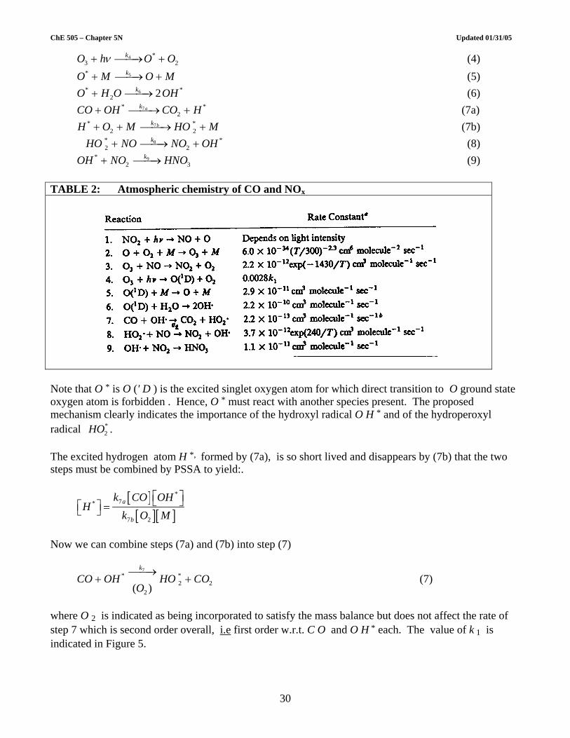
ChE 505 – Chapter 5N Updated 01/31/05
(4) 4 *3 2
kO h O Oν+ ⎯⎯→ +
(5) 5* kO M O M+ ⎯⎯→ + (6) 6* *
2 2kO H O OH+ ⎯⎯→ (7a) 7*
2akCO OH CO H+ ⎯⎯→ + *
*2 (7b) 7*
2bkH O M HO M+ + ⎯⎯→ +
8* *2 2
kHO NO NO OH+ ⎯⎯→ + (8) (9) 9*
2 3kOH NO HNO+ ⎯⎯→
TABLE 2: Atmospheric chemistry of CO and NOx
Note that O * is O (' D ) is the excited singlet oxygen atom for which direct transition to O ground state oxygen atom is forbidden . Hence, O * must react with another species present. The proposed mechanism clearly indicates the importance of the hydroxyl radical O H * and of the hydroperoxyl radical . *
2HO The excited hydrogen atom H *, formed by (7a), is so short lived and disappears by (7b) that the two steps must be combined by PSSA to yield:.
[ ]
[ ][ ]
*7*
7 2
a
b
k CO OHH
k O M
⎡ ⎤⎣ ⎦⎡ ⎤ =⎣ ⎦
Now we can combine steps (7a) and (7b) into step (7)
(7) 7
* *2
2( )
k
CO OH HO COO
⎯⎯→+ 2+
where O 2 is indicated as being incorporated to satisfy the mass balance but does not affect the rate of step 7 which is second order overall, i.e first order w.r.t. C O and O H * each. The value of k 1 is indicated in Figure 5.
30

ChE 505 – Chapter 5N Updated 01/31/05
FIGURE 5: Comparison of calculated diurnal variation of NO2, photolysis rate with experimental measurements of Zafonte et al. (1977) in Los Angeles. Reprinted with permission from Environmental Science and Technology. Copyright (1977). American Chemical Society.
The application of PSSA to the 4 intermediates yields *
2** ,,, HOOHOO
[ ] [ ][ ][ ] [ ] *
1 2 5 1 2 2 2 5 0OR r r r k NO k O O M k M O⎡ ⎤= − + = − + =⎣ ⎦
[ ] [ ] [ ]* ** 4 5 6 4 3 5 6 2 0OR r r r k O k M O k H O O⎡ ⎤ ⎡ ⎤= − − = − − =⎣ ⎦ ⎣ ⎦
* 6 7 8 92 0OH
R r r r r= − + − =
*2
7 8 0HO
R r r= − =
Summing the last two rates yields: [ ] [ ]* *
2
* *6 9 6 2 9 22 2
OH HOR R r r k H O O k OH NO⎡ ⎤ ⎡ ⎤+ = − = − =⎣ ⎦ ⎣ ⎦ 0
In addition, ozone can be treated as an active intermediate: [ ][ ][ ] [ ][ ] [ ]
3 2 3 4 2 2 3 3 4 3 0OR r r r k O O M k O NO k O= − − = − − = We solve now for the concentrations of all the active intermediates
[ ] [ ][ ][ ][ ]
2 23
3 4
k O O MO
k NO k=
+
[ ]
[ ]
*6 2*
9 2
2k H O OOH
k NO
⎡ ⎤⎣ ⎦⎡ ⎤ =⎣ ⎦
31

ChE 505 – Chapter 5N Updated 01/31/05
[ ][ ] [ ]
4 3*
5 6 2
k OO
k M k H O⎡ ⎤ =⎣ ⎦ +
[ ][ ] [ ]
[ ][ ]
*1 2 5
2 2
k NO k M OO
k O M
⎡ ⎤+ ⎣ ⎦=
Hence by substituting [O * ] into the expression for [O ] we get
[ ] [ ] [ ][ ] [ ] [ ] [ ][4 5
1 2 3 2 25 6 2
/k k M
O k NO O k O Mk M k H O
⎧ ⎫⎪ ⎪= +⎨ ⎬+⎪ ⎪⎩ ⎭]
Substitution of [O ] into the expression for [O 3 ] yields
[ ][ ] [ ][ ]
[ ] [ ][ ]
4 5 31 2
5 6 23
3 4
k k M Ok NO
k M k H OO
k NO k
++
=+
Solving for [O 3 ] we get
[ ] [ ][ ]
1 23
3 4
k NOO
k NO k a=
+
where [ ][ ]5
6 2
1
1a
k Mk H O
=+
which is constant at constant relative humidity. Now we also get
[ ][ ]
[ ][ ] [ ]( )
4 3 1 4 2*
6 2 6 2 3 4
k O k k NO aO a
k H O k H O k NO k a⎡ ⎤ = =⎣ ⎦ +
[ ][ ] [ ]( )
4 3* 1 4
9 2 9 3 4
2 2a k O a k kOHk NO k k NO k a
⎡ ⎤ = =⎣ ⎦ +
etc. The dynamics of the system is now described by:
[ ]21 3 8 9
d NOr r r r
dt= − + + −
32

ChE 505 – Chapter 5N Updated 01/31/05
[ ]
[ ]1 3
7
d NOr r r
dtd CO
rdt
= − −
= −
8
Upon substitution of the rate forms, and elimination of the concentrations of the intermediates, we get:
[ ] [ ] [ ]( )[ ]
1 4 7 9 22
3 4
2 / 3k k a k CO k NOd NOdt k NO k a
−=
+
[ ] [ ] [ ]( )[ ]
1 4 2 7 9
3 4
2 /k k a NO k CO kd NOdt k NO k a
−=
+
[ ] [ ][ ]
1 4 7 9
3 4
2 /d CO k k k a CO kdt k NO k a
= −+
with initial conditions at
[ ] [ ][ ] [ ][ ] [ ]
2 20o
o
o
t NO N
NO NO
CO CO
= =
=
=
O
The above equations certainly can be integrated on any computer. Before doing so an approximate analysis is in order. Examination of Table 2 reveals [ ]3k NO k a>> 4 for all levels of [N O ] concentrations of interest. Then
[ ] [ ][ ]
[ ][ ]
1 2 1 23
3 4 3
k NO k NOO
k NO k a k NO= =
+
as found before for the simple mechanism consisting of only 3 steps. This part of the cycle can be represented as follows:
2,
2 3
hv O
NO NO O⎯⎯⎯→
+←⎯⎯
Photolysis generates O and N O 2 which with O 2 results immediately in N O + O 3. Ozone reacts with N O to regenerate N O 2. When C O is present the above cycle is modified as N O can be converted back to N O 2 via the hydroperoxyl radical i.e step 8
33

ChE 505 – Chapter 5N Updated 01/31/05
3
,
2
2
ONONOOhv
+⎯⎯←
⎯⎯ →⎯
*2HO
But the radical gets converted to OH *, which with CO regenerates the radical. Hence, one has two cycles - the fast cycle
*2HO *
2HO*
2 3, , cycle and a slower , ,NO NO O CO OH HO*2
3
,
22
2
ONONOO
Ohv
+⎯⎯⎯←⎯⎯ →⎯
−
*2
* HOOHCO ⎯→⎯+
The CO/NO x reaction mechanism is a chain reaction with OH * as the chain carrier. The chain length Lc of such a reaction is defined as the number of propagation steps occurring for each termination step. In our mechanism
[ ][ ]
78 7
9 9 9 2c
k COr rLr r k NO
= = =
The role of the CO slow cycle is to slowly change (i.e increase) the [NO2] concentration and hence increase [O3 ] concentration which is still given by its pseudo steady state value. Because of the extreme rapidity of NO 2/O3 cycle it is the external independent paths that affect [NO2] which determine maximum [O3] levels. For completion of the ozone story one would need to include reactions of organic compounds and the effect of particulate matter (aerosol) as potential catalyst. This is beyond the scope of illustration of the PSSA assumption. The same rules as illustrated here can be applied.
34

THEORY OF ELEMENTARY
REACTIONS
(CHE 505)
M.P. Dudukovic
Chemical Reaction Engineering Laboratory
(CREL),
Washington University, St. Louis, MO

ChE 505 – Chapter 6N Updated 01/31/05
6. THEORY OF ELEMENTARY REACTIONS 6.1 Collision Theory Collision theory is the extension of the kinetic theory of gases in predicting reaction rates of a bimolecular gas phase reaction of the type: A + A → P (1) A + B → P (2) It is assumed that the reaction rate expressed in terms of disappearance of molecules of A is given by:
− ?r Amolecules
cm 3 s⎛
⎝ ⎜ ⎞
⎠ ⎟ =2 f Z A A for reaction(1)
A factor two appears on the right hand side of eq (1) because for each collision two molecules of A disappear.
− ?r A = − ?r Bmolecules
cm 3 s⎛
⎝ ⎜ ⎞
⎠ ⎟ = f Z A B for reaction (2)
where ZA B - is the total number of collisions between molecules A and B in 1 cm3 of reaction mixture per second (frequency of collision per 1 cm3) Z A A - is the total number of collisions among the molecules A in 1 cm3 per second f - the fraction of molecules that possess the required excess energy for reaction i.e the fraction of molecules that upon collision will react. The kinetic theory of gases postulates that the collision frequency Z A B is proportional to the size of the "target", to the relative mean velocity u A B ,, and to the number concentrations of both molecular species. The size of the "target" is interpreted as the maximum area perpendicular to the trajectory of the moving A (or B ) molecule which when it contains a B (or A ) molecule will lead to an inevitable collision of the two. (See Figure 1).
1

ChE 505 – Chapter 6N Updated 01/31/05
FIGURE 1: Frequency of collisions: molecule A is moving with speed u relative to B. In unit time the sphere of radius rA + rB has swept out a volume π rA + rB( )2
u and has
encountered molecules of B. π rA + rB( )2uNB
r
B
B
ur
A
A
B
r
Thus
" t arget area" = π d A B
2 = π σ A B2
where d A B = d A + d B2
= dAB is the radius of collision area
d A, d B can be interpreted as equivalent molecular diameter of molecule A and B , respectively, if the molecules are viewed as hard spheres according to the classical collision theory. d A, d B can also be viewed as diameters in space of the sphere within which the attraction forces of A or B would force a collision. The mean relative velocity is given by the kinetic theory as
u A B =8k B Tπ µ AB
⎛
⎝ ⎜
⎞
⎠ ⎟
1/2
(3)
where k B = 1.38062 x 10⁻²³JK-1 is the Boltzmann's constant.
µ A B =m A m B
m A + m B− reduced molecular mass (4)
with m Ag
molecule⎛ ⎝
⎞ ⎠ being the molecular mass of A , m B the molecular mass of B .
The number concentrations are:
2

ChE 505 – Chapter 6N Updated 01/31/05
N Anumber of molecules of A
c m 3
⎛ ⎝ ⎜ ⎞
⎠ ; N B
number of molecules of Bcm 3
⎛ ⎝ ⎜ ⎞
⎠
The fraction of molecules having sufficient energy levels to react are given by the Boltzmann factor f = e − E m /k B T where E m is the difference in energy of an "excited" and "base" molecule. The rate then becomes:
− ?r Amolecules
c m 3 s⎛ ⎝ ⎜ ⎞
⎠ = πσ A B
2 8k BTπ µ AB
e − E m/ k B T N A N B (5)
We want to express the rate in mollit s
⎛ ⎝ ⎜ ⎞
⎠ and the concentrations in
mollit
⎛ ⎝ ⎜ ⎞
⎠ . Then:
N a
10 3 C A =N A ;N a
10 3 C B = N B
− r Amoleslit s
⎛ ⎝ ⎜ ⎞
⎠ x
N a
10 3 = − ?r Amolecules
cm 3 s⎛ ⎝ ⎜ ⎞
⎠
Also
k B N a = R ; µ A B N a = M A B =M A + M B
M A M B
⎛
⎝ ⎜ ⎞
⎠ ⎟
−1
where N a is the Avogardro's constant
N a = 6.02217 x 10 23 molecules
moleM A ,M B − molecular weights
The expression for the rate finally becomes
− r Amolelit s
⎛ ⎝ ⎜ ⎞
⎠ = σ A B
2 8π R TM A B
e −E /RT N a10 3
k1 2 4 4 4 4 4 3 4 4 4 4 4
C A C B (6)
Thus
3
k = k o T 1/2 e −E/ RT (7a)

ChE 505 – Chapter 6N Updated 01/31/05
k o = σ AB2 8 π R
M AB
N a10 3 (7b)
Collision theory predicts the dependence of the rate constant on temperature of the type T 1/2 e - E / R T and allows actual prediction of the values for the frequency factor from tabulated data. For reaction of type (1)
Z A A =12
πσ A2 8k B T
π µ AA
⎛
⎝ ⎜ ⎞
⎠ ⎟
1/ 2
N A2 (8)
Factor 12
is there since all the molecules are the same and otherwise the collisions would have been
counted twice. This factor is offset by the 2 in the rate expression which simply indicates that in every collision two molecules of A react.
Now µ A A =m A2
− ?r Amolecules
c m 3 s⎛ ⎝ ⎜ ⎞
⎠ = σ A
2 16π k B Tm a
⎛
⎝ ⎜ ⎞
⎠ ⎟
1/ 2
e − E m/ k B T NA2 (9a)
− r Amoleslit s
⎛ ⎝ ⎜ ⎞
⎠ = 4σ A
2 πRMA
N a
10 3 T 1/ 2
k o coll
1 2 4 4 4 3 4 4 4
e − E / RT
k1 2 4 4 4 4 4 3 4 4 4 4 4
CA2
(9b)
Some predictions of the collision theory will be compared later to transition state theory. Note: T 1/2 dependence is almost entirely masked by the much stronger e - E / R T dependence. Thus Arrhenius form is a good approximation. The relationship to Arrhenius parameters is:
k o Arr
= k o colle T ( )1/2
(10a)
E Arr = E coll +12
R T (10b)
Original comparison of the collision theory prediction with experimental values for the reaction 2 H I → H 2 + I 2 resulted at 556K in k predicted = 3.50 x 10⁻⁷ (L/mol s) as opposed to kexp = 3.52 x 10⁻⁷ (l/mol s). This proved to be an unfortunate coincidence as later it became evident that predictions based on collision theory can lead to gross discrepancies with data. For example, for more complex gas molecules predicted pre-exponential factors are often order of magnitude higher than experimental values and severe problems arise for reactions of ions or dipolar substances. The modifications to the collision theory recognize that the collision cross-sectional area is not a
4

ChE 505 – Chapter 6N Updated 01/31/05
constant, but a function of energy, introduce a steric factor and acknowledge that molecules do not travel at the same speed but with a Maxwell-Boltzmann distribution of velocity! If one considers just the translational energy, ε t , one can argue that the rate constant can be predicted from
k T( ) = (8
πµ k T( )3 )1/ 2 ε to
∞
∫ σ ε t( )e− ε t / kT d ε t (11)
Similar but more complex expressions can be derived accounting for rotational and vibrational energies. Modern analytical tools allow measurement of effective reaction cross-section when reactant molecules are in prescribed vibrational and rotational states. When such information is available collision theory in principle leads to the 'a priori' prediction of the rate constant. Example 1. Using collision theory estimate the specific rate constant for the decomposition of H I at
321oC, σ H I = 3.5 A, E = 44000calmol
. Experimentally the rate constant is found to be
k = 2.0 x 10 −6 litmol s
⎛ ⎝ ⎜ ⎞
⎠ . Collision theory prediction is:
k = 4σ H I2 π RT
M H I
N a
103 e − E / RT
k = 4 x 3.5 x 10 −8( )2 π 8.314 x 10 7 x 273 + 321( )127.9
e− 44000
1.987 x 594 x6.023 x 10 23
103
σ H I = 3.51 x 10 −8 cm ; R = 8.314 x 10+7 erg / mol K
T = 273 + 321 = 594 K , M H I = 127.9
N a = 6.023 x 10 23 molecules / mol
k = 6.63 x 10 −6 lit
mol s← collision theory estimate
k = 2.0 x 10 −6 litmol s
← experimental value
Collision theory usually gives the upper bound of the rate constant. ________________________________________________________________________ 6.2 Classical Transition State Theory (CTST) This is the most promising of the rate theories and deals again with elementary reactions. However, even an elementary reaction is not viewed any more to occur exactly in one step (this shows how flexible the definition of elementary reactions has become since they are supposed to occur in one step). According to transition state theory every elementary reaction proceeds through an activated complex - a transition state.
reac tants( )⇔ transition state( ) ⇔ products( )
A + B ⇔ Z * ⇔ Q + P (12)
5

ChE 505 – Chapter 6N Updated 01/31/05
The transition state is a little more than the fraction of excited (energized) reactant molecules as in Arrhenius or collision theory. Its structure is neither that of the reactants nor of products, it is someplace in between and its concentration is always orders of magnitude lower than that of reactants or products. The transition state can either be formed starting solely with reactant molecules from the left or with product molecules from the right. The energy picture is as shown in Figure 2. FIGURE 2: Energy Diagram (Simplified for the Classical Transition State Theory)
E f
Reaction Coordinate
Eoz
−∆H Eb
Eob*
Eof*
Eor
ZZ* #
Energy Level
EopBase Level
Eor - energy level of reactants Eop - energy level of products Eoz - energy level of transition state Eof* - activation barrier for forward reaction Eob* - activation barrier for reverse reaction ∆ Ho - heat of reaction E o f
* = E f = E o z − E o R
E o b* = E b = E o z − E oP
∆ H = E o p − E o R = E o z − E b( )− E oz − E f( )∆ H = E f − E b
When the overall system, i.e reactants and products, is in equilibrium, clearly the net rate of reaction is zero, i.e r = r f - r b = 0 However, even in overall equilibrium a certain number of reactant molecules gets transformed per unit
6

ChE 505 – Chapter 6N Updated 01/31/05
time into the transition state, and the same number gets transformed from transition state to reactants as required by the principle of microscopic balancing. At the same time a certain rate of exchange exists between transition state and products which is balanced by the exchange between products and transition state. That exchange rate at overall equilibrium is proportional to ν C z where ν is the frequency of
occurrence of exchange 1s
⎛ ⎝
⎞ ⎠ and C z the number concentration of the transition state.
The three fundamental assumptions of transition state theory are: 1. The rate of reaction is given by r = ν C z (13) even when the system is removed from equilibrium i.e when there are no products, or products are
being removed, or they are present in amount less than required by equilibrium. This is equivalent to assuming that the equilibrium between the transition states and reactants is always established.
2. The frequency ν involved is a universal frequency, it does not depend on the nature of the
molecular system and is given by
ν =k B Th p
(14)
where k b = 1.38062 x 10⁻²³ JK-1 Boltzmann's constant h p = 6.6262 x 10⁻³⁴ Js Planck's constant T (K) - absolute temperature 3. The reaction system is "symmetric" with respect to the transition state and the above is also true
when starting from products to make reactants (from right to left). A more rigorous treatment is outlined in appropriate textbooks on kinetics (e.g. see Laidler, Chemical Kinetics). This is a very bold assumption asserting that the equilibrium rate of exchange is equal to the rate for the system out of equilibrium. If we refer to Figure 3, the above assumptions indicate that once reactant molecules have reached the col of the activated complex (transition state) from the left there is no going back and they get converted to products. Similarly, the product molecules that reach the col from the right cannot turn back and do get transformed to reactants.
7
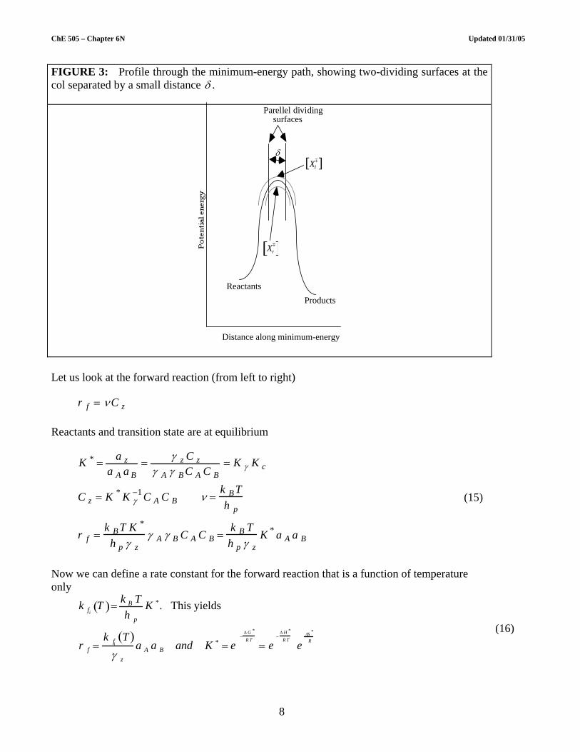
ChE 505 – Chapter 6N Updated 01/31/05
FIGURE 3: Profile through the minimum-energy path, showing two-dividing surfaces at the col separated by a small distance δ .
Xr
m[ ]
δ
ProductsReactants
Xl
m[ ]
Parellel dividingsurfaces
Distance along minimum-energy Let us look at the forward reaction (from left to right) r f = ν C z Reactants and transition state are at equilibrium
K * = a za A a B
= γ z C zγ A γ B C A C B
= K γ K c
C z = K * K γ−1 C A C B ν =
k B Th p
r f =k B T K *
h p γ zγ A γ B C A C B =
k B Th p γ z
K * a A a B
(15)
Now we can define a rate constant for the forward reaction that is a function of temperature only
k fiT( )= k B T
h p
K *. This yields
r f =k fi
T( )γ z
a A a B and K * = e−
∆ G *
R T= e
−∆ H *
R Te
∆S *
R
(16)
8

ChE 505 – Chapter 6N Updated 01/31/05
Similarly for the reverse reaction r b = ν C z , and the equilibrium between transition states and products is always established.
K ≠ = γ z C zγ Q γ P C Q C P
C z =a Q a p
γ zK ≠
K≠ = e− ∆ G ≠
RT
= e− ∆ H ≠
R T
e∆ S≠
R
The reverse rate is now expressed by
r b =k bi T( )
γ z
a Q a P where k bi T( )=k B Th p
K ≠ (17)
In the above ∆ G *,∆ H *,∆ S * and ∆ G ≠, ∆ H ≠, ∆ S ≠ are the Gibbs free energy, heat of reaction, and change in entropy for formation of the transition state starting from reactants and products, respectively. The net rate of reaction then is
r = rf − rb =1γ z
k fi aA aB − kb iaQaP[ ] or
r =kBThpγ z
K*aAaB − K≠
aQaP[ ]=koThpγ z
e− ∆H *
RT eAS*
R aAaB − e− ∆H ≠
RT e− ∆S≠
R aQaP
⎡
⎣ ⎢
⎤
⎦ ⎥ (18)
At equilibrium r = 0 so that the equilibrium constant K for the reaction is recovered:
K =aQaP
aAaB
= e− ∆H *−∆H≠
RT e∆S*− ∆S≠
R = e− ∆G* −∆G≠
RT
Therefore, the following equations hold:
∆ H * − ∆ H ≠ = ∆ H° − heat of reaction
∆ S * − ∆ S ≠ = ∆ S ° − entropy due to reaction
∆ G * − ∆ G ≠ = ∆ G ° − Gibbs free energy change due to reaction
∆ H * = E f ∆ H ≠ = E b
Let us call k rate constants which are functions of T only. f T( ) = k f i
k b T( )= k b i
[ PQbfBAfiz
aakaakri
−=λ1 ] (19)
9

ChE 505 – Chapter 6N Updated 01/31/05
We usually express the rate in the form: r = k f C A C B - k b C Q C P (20) This gives the relationship:
k f = k f i
γ A γ Bγ z
k b = k b i
γ Q γ P
γ z (21)
This is a very important result of the transition state theory. It tells us that whenever we write and evaluate a rate expression with its driving force being expressed in molar concentrations the rate constants, k f , k b , etc. that appear in such expressions are not only functions of temperature but also could be functions of pressure and concentration. This is obvious from the above since k are functions of temperature only but
f i, k b i
γ A,γ B, γ Q, γ P ,γ z can also be functions of pressure or concentration. The above relationship between rate constants k f , k b in nonideal systems for rates whose driving force is as usual expressed in concentrations, and the ideal rate constants k which would be observed in a system with all activity coefficients of unity, is frequently used to correct the constants for pressure effects in gas reactions or for concentration effects in ionic solutions.
f i, k b i
Relationship to Arrhenius parameters k o Arr
e − E Arr / RT is:
k o Arr= e
k B T γ zh p
⎛
⎝ ⎜
⎞
⎠ ⎟ e ∆ S ° /R ; E Arr = ∆ H * + R T (22)
Note: Sometimes transition state theory is interpreted by asserting that the rate is proportional to the product of the universal frequency and the activity of the transition state (rather than to its concentration). This would lead essentially to the same expressions as shown above except that γ z would not appear, i.e wherever it appears it would be replaced by unity. ________________________________________________________________________ Example.2 Estimate the rate constant for decomposition of methyl aride CH3N3 by transition state theory at 500K, given ∆ H * = 42 ,500 cal / mol , ∆ S * = 8.2 cal / mol K.
k =k B Th p
e− ∆ H *
R T
e∆ S*
R
k =
1.38062 x 10 −23 x 5006.6262 x 10 − 34 e
−42500
1 .987 x 500
e8 .2
1.987
k = 1.705 x 10 −4 s −1
10

ChE 505 – Chapter 6N Updated 01/31/05
When we use transition state theory to calculate the rate constant for reaction of the type A = B there is no ambiguity as to the units of the rate constant. However, when we deal with bimolecular reactions of the type A + B ⇔ P + Q and
k f =
k B Tν}
h p
Kd* ; kh =
k B Tν}
h p
K d≠
the units of the rate constants are not governed by the kinetic factor ν1s
⎛ ⎝
⎞ ⎠ but rather by the
thermodynamic factor , i.eK d* and K d
≠ by the choice of standard states for calculation of upon which the calculation of these parameters ∆ G * and ∆ G ≠ K d
*,K d≠ are based. If concentration is
chosen for the driving force in the rate expression then d = c and Kd* = Kc
* = Cz* / CACB , if pressure is
chosen then d = p and . Similarly, Kp* = Pz
* / pA pB
. Kc≠ =C z
* /C pCq, and K p≠ = Pz
* / PpPq
It is useful therefore to review the use of standard states and relationships between thermodynamic quantities at this point. For a general reaction
j=1
s
∑ ν j A j = 0
The thermodynamic quantities are generally tabulated for standard states of 1 atm and ideal gas. Frequently we want to transform these to standard states expressed in concentration
units, generally 1
K, ∆ H °,∆ G °,∆ S °,C p°
mollit
1 M( ) .
________________________________________________________________________ Example. 3
When using transition state theory for a bimolar reaction for which , since two moles of
reactant give one mole of transition complex, and when the quantities are based on standard states at 1 atm of ideal gases , then from transition theory
υ jj=1
S
∑ = −1
K *,∆ H *,∆ S *
∆ H p
* = ∆ Hc* − RT .
k p =k B Th p
e∆S p
*
R e−
∆ H p*
RT atm −1,s −1( )
Compared with Arrhenius equation
11

ChE 505 – Chapter 6N Updated 01/31/05
k p f Arr= k p o
' e − Ep' /R T atm−1,s −1( )
yields the frequency factor
k p o
' = ek B T h p
e∆ S p
*
R T atm −1,s −1( ) and activation energy E p
' = ∆ H * + RT = ∆ U * Compared with Arrhenius equation in concentration units
k c = k c oe −E c /R T lit
mol, s −1⎛
⎝ ⎞ ⎠
it gives the frequency factor:
k c o= k p o
' R' T( ) e = e 2 k BT h p
R'T e∆ S p
*
R
= e2 k B T h p
e∆ S p
* + Rln R'TR = e2 k B T
h pe
∆ Sc*/R
since ν j = − 1∑ going from two reactant molecules to one molecule of the transition state The activation energy is E c = E p
' + RT = ∆ H p* + 2 RT = ∆ U * + R T
________________________________________________________________________ Example. 4. The homogeneous dimerization of butadiene (CH2=CH-CH=CH2) has been studied extensively. An experimental rate constant based on disappearance of butadiene was found as:
k = 9.2 x 10 9
k o
1 2 4 3 4 e −23960/ RT cm 3
mol s⎛
⎝ ⎜ ⎞
⎠ ⎟
a) Use collision theory to predict a value of k o at 600 K and compare with experimental value of 9.2 x 10⁹. Assume effective collision diameter 5 x 10⁻⁸ cm.
k ocm 3
mol s⎛
⎝ ⎜ ⎞
⎠ ⎟ = 4σ B
2 π RTM B
N a e
k o = 4 x 5 x 10 −8( )2 π x 8.314 x 10 7 x 60054
x 6.023 x 10 23 e
12

ChE 505 – Chapter 6N Updated 01/31/05
k o = 8.81 x 10 14 cm 3
gmol s⎛
⎝ ⎜ ⎞
⎠ ⎟ ← collision theory prediction
k o = 9.2 x 10 9 cmgmol s
⎛ ⎝ ⎜ ⎞
⎠ ← experimental value
b) Use transition-state theory to predict k o at 600 K and compare to experimental value. Assume the
following form of the transition state (a hint from a friendly chemist!) ' ' CH2 -CH=CH-CH2-CH2-CH-CH=CH2
k o = e 2 k B Th p
R'T e∆ S p
*
R= e 2 k B T
h pe ∆Sc
* /R
∆ S c* = ∆ S p
* + Rln R'T
We have to calculate the change of entropy for the formation of transition state from reactants. To do this the group contribution method and appropriate tables are used. [D.A. Hougen and K.M. Watson "Chemical Process Principles" Vol. II: pp 759-764 Wiley, NY, 1947; or S.W. Benson "Thermochemical KInetics, 2nd ed. - Methods for the Estimation of Thermochemical Data and Rate Parameters", Wiley, NY 1976]. Using Benson's Tables (attached) we get for CH2=CH-CH=CH2
S ° = 2 x 27.61 + 2 x 7.97 = 71.16cal
mol K
T 300 400 500 600 Cp 18.52 22.78 26.64 30.00
For CH2-CH=CH-CH2-CH2-CH-CH=CH2 using the contributions of CH2 to be between those for -CH3 and -CH2 radical we get So = 110.995 cal/mol K.
T 300 400 500 600 Cp 40.0 49.42 57.82 65.02
Then
∆ S T* = ∆ S o
* +∆ C p
TT o
T
∫ d T
∆ S T* = ∆ S o
* + 12
∆ C p T o( )T o
+∆ C p T 1( )
T 1+
∆ C p T 2( )T 2
+ 12
∆ C p T 3( )T 3
⎡
⎣ ⎢ ⎤
⎦ ⎥ ∆ T
13

ChE 505 – Chapter 6N Updated 01/31/05
∆ S T* = 110.995−2 x 71.16( ) +
12
40.00 − 2 x 18.52300
+ 49.42 − 2 x 22.78400
+
57.82 − 2 x 26.64500
+12
65.02 − 2 x 30.00600
⎡
⎣
⎢ ⎢
⎤
⎦
⎥ ⎥
x 100
∆ S T* = − 31.325 + 2.785 = − 28.54
calmol K
k c o
= e 2 1.38062 x 10 23 x 6006.6262 x 10 34 e
−28.54 +1.987 ln 0.0821 x 600( )
1.987 x 10 3
k c o= 2.63 x 10 12 cm 3
gmol s⎛
⎝ ⎜ ⎞
⎠ ⎟ ← transition state theory prediction
k c o= 9.2 x 10 9 cm 3
gmol s⎛
⎝ ⎜ ⎞
⎠ ⎟ ← experimental value
A closer prediction but still an upper bound. Remember the structure of the transition state was only hypothesized and all thermodynamic quantities only estimated. Table 1: Some useful orders of magnitude Quantity Expression Order of Magnitude Units
8k B Tπ µ A B
⎛
⎝ ⎜
⎞
⎠ ⎟
1/2
5 x 10⁴ (cm/s) mean molecular velocity
universal frequency k B Th p
1013 (1/s)
collision frequency gas-gas 10-10 (cm3/s - molecule) π σ AB2 u A B
collision frequency gas-solid u 4
104 (cm/s)
It is instructive to gain an insight into the order of magnitude of some important quantities by examining Table 1 above, and to learn a little more about the comparison in prediction of the TST and collision theory from Table 2. ___________________________________________________________________________________ Table 2: Comparison of Theories Reaction Logarithm of kco Observed Transition State Collision Theory Theory NO + O 3 → NO 2 + O 2 11.9 11.6 13.7 NO 2 + O 3 → NO 3 + O 2 12.8 11.1 13.8 NO 2 + F 2 → NO 2 F + F 12.2 11.1 13.8 NO 2 + CO → NO + CO 2 13.1 12.8 13.6 F 2 + C lO 2 → FC lO 2 + F 10.5 10.9 13.7 2C lO → C l 2 + O 2 10.8 10.0 13.4 Transition theory seems to give consistently better predictions.
14

ChE 505 – Chapter 6N Updated 01/31/05
6.3. Transition State Theory explained by Statistical Mechanics In this section, we will investigate the relationship between molecular level concepts and thermodynamic properties. In order to be able to start looking at molecular level, we will introduce partition functions that describe a specific system using statistical mechanics. Let’s start with a few definitions. An ensemble is a collection of subsystems that make up the thermodynamic state. Different ensembles are obtained depending on the intensive (e.g. temperature (T)) or extensive (e.g. volume (V)) variables that define the thermodynamic state. Figure 4 shows an example of an ensemble that has 16 states. If there is no material exchange between the states, composition (N) is constant for each state. In a microcanonical ensemble, V, energy (E) and N are kept constant.
1 NVE 2 NVE 3 NVE 4 NVE 5 NVE 6 NVE 7 NVE 8 NVE 9 NVE 10 NVE 11 NVE 12 NVE 13 NVE 14 NVE 15 NVE 16 NVE
FIGURE 4. An example of a microcanonical ensemble with 16 states each at constant N, V and E Microcanonical ensemble is therefore isolated since each state is at the same energy and no energy transfer occurs between the states. In a canonical ensemble, the states are not isolated and T is fixed instead of E. By this way, E may be transferred as heat. If the states are not closed but open to material exchange and chemical potential (µ) , V and T are fixed, the ensemble is defined as grand canonical ensemble. Finally, the ensemble is called isothermal-isobaric for states with constant N, T, and pressure (P). In statistical mechanics, each ensemble can be connected to the classical thermodynamical information using partition functions. The derivation for the connectivity equations are explained in detail in statistical mechanics books (e.g. Donald A. McQuarrie, “Statistical Mechanics”, Harper Collins Publishers, NY, 1976 and M.P. Allen, D.J. Tildesley, “Computer Simulation of Liquids”, Clarendon Press, Oxford, 1997) Table 3 summarizes the connectivity equations between the micro-level partition functions and the macro-level classical thermodynamic equations. Table 3. Connectivity equations Ensemble Thermodynamic Quantity Equation microcanonical S
NVEBQkS = canonical A
NVTB
QTk
A ln−=
grand canonical pV VTB QTkpV µln=
isothermal-isobaric G NPTB QTkG ln−=
In the table Q represents the partition function for the ensemble. (e.g. QNVE represents partition function for the microcanonical ensemble where N,V, and E are constant.) If the molecules that make up the system are independent of each other as in an ideal gas at the canonical ensemble, the partition function, Q can further be divided into individual molecular partition functions as:
15

ChE 505 – Chapter 6N Updated 01/31/05
!N
qQN
= (23)
The molecular partition function itself consists of different contributing partition functions of different contributing partition functions arising from different modes of motion, mainly translational, rotational, vibrational, electronical and nuclear. In other words, (24) electronicnuclearlvibrationarotationalnaltranslatio qqqqqq = Let’s focus on the individual contributions: Translational contribution:
2/3
2
2⎟⎟⎠
⎞⎜⎜⎝
⎛=
p
Bnaltranslatio h
TmkVq π (25)
with m being the molecular mass and being the Plank constant = 6.62608 x 10⁻³⁴ Js ph Rotational contribution:
∑+
−
+=J
TkhcBJJ
rotationalBeJq
)1(
)12(1σ
(26)
with J = 0,1,2,…., σ = symmetry number, 1 for heteroatomic molecules and 2 for homoatomic molecules c = speed of light B = rotational constant for each molecule (cm-1) Rotational contribution is usually approximated by Eq. 27.
hcB
Tkq Brotational σ
≈ (27)
Vibrational contribution:
Tkh
Tkh
lvibrationa B
B
eeq ν
ν
−
−
−=
1
2/
(28)
where πµ
ν21
2/1
⎟⎟⎠
⎞⎜⎜⎝
⎛=
k (29)
with k being the force constant of the molecule and µ being the reduced mass.
16

ChE 505 – Chapter 6N Updated 01/31/05
Nuclear contribution:
nuclearq is taken as the degeneracy of the ground nuclear state. It is usually omitted in the calculations because for most cases, nuclear state is not altered for states of interest. Electronic contribution: (30) )(efqelectronic = The electronic partition function is basically given as a function of degeneracy of the electronic ground state and is equal to 1 for most cases. Rate Constant Related to Molecular Partition Functions If we look at our reaction Eq (12) and express the equilibrium constant, K using partial pressures, we can see how molecular partition functions correlate with transition state theory.
reac tants( )⇔ transition state( ) ⇔ products( )
A + B ⇔ Z * ⇔ Q + P (12)
From classical thermodynamics: (31) pVAG += Combining and keeping in mind that NTknRT B= (32)
⎟⎠⎞
⎜⎝⎛−=⎟
⎠⎞
⎜⎝⎛−
=+−+−=+−−=+−=
NqnRT
NqTNk
nRTNNNTkqTNknRTNqNTknRTNqTkG
B
BBB
N
B
lnln
)ln(ln)!lnln(!
ln (33)
We also know that (34) fi
s
j jr GG ∆=∆ ∑ =1ν
Then combining with Eq. 33
oTi
Tifi UNq
RTGGG +⎟⎠⎞
⎜⎝⎛−=+=∆ ln
0 (35)
Note that we lost the n factor of Eqn (35) since G is in terms of molar quantity. If we select our reference system as T = 0, then G = U. Combining Eqs (34) and (35) gives
17

ChE 505 – Chapter 6N Updated 01/31/05
01ln E
Nq
RTG s
jj
r
j
∆+⎟⎟⎠
⎞⎜⎜⎝
⎛−=∆ ∑ =
ν
(36)
We also know that (37) KRTGr ln−=∆ Finally we have K in terms of q by
∏ ∆−⎟⎟⎠
⎞⎜⎜⎝
⎛=
j
RTEj eNq
Kj
/0
ν
(38)
6.4 Some Consequences of TST 6.4.1 Rate Constants in Dilute Strong Electrolytes Debye-Hüchel theory relates the activity coefficient of dilute strong electrolytes with the ionic strength I of solution and with the charge of the ion in question:
IAZn jj2−=γl (39)
Where ion of charge jZ j −
jγ - activity coefficient of ion
∑=
=s
jjj ZCI
1
2
21 - ionic strength (40)
- molar concentration of j ion jC - constant (A ≈ 0.51 for water at 25ºC) A For reaction of A
ZA
+ BZ B
→ Z * (Z A +Z B ) (41)
the transition state theory predicts:
k 1c = k 1γ A γ B
γ Z* (42)
Clearly the transition state must have a charge of Z A + Z B in order to satisfy the law of conservation of charge. Taking logarithms
18

ChE 505 – Chapter 6N Updated 01/31/05
l nk 1c = ln k 1 + ln γ A + ln γ B − ln γ Z*
= l nk 1 − A I Z A2 + Z B
2 − Z A + Z B( )2[ ] (43)
l nk 1c = ln k 1 + 2 A Z A Z B I
This equation gives excellent agreement with experimental data and is very useful for correlating liquid phase reaction data. 3.2.2 Pressure Effects in Gas Phase Reactions For gases
a j = f j = φ j P j = γ j C j =γ j P j
Z j RT
Z j − compressibility factor of j
γ j − activity coefficient of j
P j − partial pressure of j
C j − molar concentration of j
φ j − fugacity coefficient of j
f j − fugacity of j
(44)
From the above γ j = φ j Z j RT (45) For a reaction A + B → Z *
k c = k
γ A γ Bγ Z
* = kφ A Z A RT( )φ B Z B
φ Z Z Z
k c = k φ A φ Bφ Z
Z A Z BZ Z
RT (46)
At sufficiently low pressures φ j→ 1, Z j →1
k ck
⎛ ⎝
⎞ ⎠ low pressure
= RT (47)
At high pressure
k ck
⎛ ⎝
⎞ ⎠ high P
= RTφ A φ B
φ Z
Z A Z BZ Z
(48)
19

ChE 505 – Chapter 6N Updated 01/31/05
Thus the ratio
k c, high Pk c,low P
⎛
⎝ ⎜ ⎞
⎠ ⎟ =
φ A φ Bφ Z
Z A Z BZ Z
(49)
In the case of a reaction 2 A →
k c high Pk c low P
⎛
⎝ ⎜ ⎞
⎠ ⎟ =
φ A2
φ Z
ZZ assu ming Z A ≈ Z Z (50)
The variation of the thermodynamic properties with pressure was calculated for H I decomposition (2 H I → I c + H c ). The above equation agreed excellently with all experimental data up to 250 atm which led to density variations of 300. 6.4.3 Dependence of Rate Constants on Temperature and Pressure In Chain Reactions So far we have treated only simple reactions (often elementary ones) and their rate constants. Let us take a look at more complex overall reactions - say in free radical polymerization:
r pol = k pk d fk t
k1 2 4 3 4
CM C I (51)
using Arrhenius form for k and each other constant we get tdp kkk ,,
RT
EEEfn
kk
knkntdp
t
dp
o
o
o
21
21
21
2/1 −+−+
⎥⎥
⎦
⎤
⎢⎢
⎣
⎡
⎟⎟⎠
⎞⎜⎜⎝
⎛= lll
(52)
k o = k p o
k d o
k t o
⎛
⎝ ⎜
⎞
⎠ ⎟
1/2
E = E p +12
E d − E t( ) (53)
Range of values 30 < E d < 35 kcal/mol 5 < E p < 10 kcal/mol 2 < E t < 5 kcal/mol 17 < E < 26
E ≈ 20kcalmol
Polymerization rate increases with temperature. However the degree of polymerization X n is proportional to the following group that depends on temperature:
20

ChE 505 – Chapter 6N Updated 01/31/05
X n ∝k p
k d k t( )1/2 (54)
The activation energy for the degree of polymerization is then given by
X n = X n oe
−E x n
RT
E x n= E p −
12
E d + E t( )− 15 < E x n
< − 6 kcal / mol
(55) (56)
Thus, degree of polymerization decreases rapidly with increasing temperature. The dependence on pressure is
d l nkdP
=− ∆V *
RT (57)
∆ V * - volume of activation, i.e change in volume in going from reactants to transition state.
∆ V R
* = ∆ V d*
2+ ∆ V P
* + ∆ V t*
2− 20 < ∆ V R
* < 15 cm 3/ gmol( ) (58)
Polymerization rate increases with pressure.
∆V X n
* = ∆V P* −
12
∆V d* + ∆V t
*(− 25 < ∆V X n
* < − 20 cm 3 / gmol()) (59)
Degree of polymerization increases with pressure
d l n X nd P
=− ∆V X n
RT (60)
6.5 Summary 1. Temperature dependence of rate constants can be represented over a limited range of temperature in a satisfactory manner by the Arrhenius equation k = k o e - E / R T 2. E, k o usually are constant within a narrow temperature range but may become functions of T in a
broader temperature range .E ∝ α + β T,k o ∝ T m 3. In case of high E ( E >> 20,000 cal) and moderate temperatures (T < 600 K) the value of E is not
affected by the choice of units for the driving force i.e C A (mol/lit) or P A (atm), etc.
21

ChE 505 – Chapter 6N Updated 01/31/05
4. In case of low E ( E < 10,000 cal) and high and moderate temperatures the value of E is greatly affected by the choice of variables for the driving force i.e C A (mol/lit) or P A (atm) etc.
5. The reaction rate can increase dramatically with temperature. The larger the E the more rapidly
the rate increases with T. FIGURE 5: Effect of Temperature on the Rate Constant
1
5
10
50
100
1,000
10,000
0 0.1 0.2 0.3 0.4 0.5 0.6 0.7 0.8 0.9 1.0
E = 80,000 E = 60,000 E = 20,000 cal/gmol
Say T = 300 KE = 10,000 cal/gmol
o
kT
kTo
1To
−1T
⎛
⎝ ⎜
⎞
⎠ ⎟ × 103
← T
E = 40,000
kT = rate constant at temperature T
kTo = rate constant at T = To = 300K = 27oC
The above figure (Figure 5) demonstrates the possible rapid rise in reaction constants and rates if activation energy is sufficiently high. The rate increases 10 times for E = 10,000 cal for a ∆ T of 50K. For the same rise in temperature the rate with E = 20,000 cal will increase 100 times. It takes only 35oK to raise a rate constant 1000 times for E = 40,000. 25oK temperature increase gives a 1000 times larger rate for E = 60,000 cal and a staggering 10,000 times larger rate for E = 80,000 cal!
6. for elementary reactors. E f − E b = ∆H o reaction For exothermic reactions ∆H ° < 0( ) E f < E b and a rise in temperature will promote more the reverse reaction and thus reduce
equilibrium conversion. This is obvious also from
dl n KdT
=∆H
RT 2 < 0.
22

ChE 505 – Chapter 6N Updated 01/31/05
∆H <O
d l n KdT
< 0 asT↑ K↓. However, forward rate rises also with T to some extent.
There always is a T optimal which balances the increased rate with more unfavorable equilibrium. 7. For endothermic reactions E f > E b , and for irreversible reactions, the higher the temperature the
higher the rate and the higher conversion is obtainable. 8. A temperature excursion of 10-20˚C can cause dramatic increases in the rate and lead to runaways
and explosion. 9. The reaction rate is so much more sensitive to temperature than to concentration. For a first order
reaction with E = 20,000 cal a rise of 50˚C in T leads to an increase of 100 times in the rate. To accomplish the same augmentation of the rate by changing concentrations we would have to increase concentration 100 times. For a 2nd order reaction with the same activation energy we would have to increase concentration 10 times. For higher activation energies the difference between temperature and concentration sensitivity of the rate is even more pronounced.
23


![Mechanism, Regioselectivity, and the Kinetics of Phosphine ... · chemistry of nucleophilic phosphine organocatalysis and re-lated reactions in general.[10] In addition, these mechanistic](https://img.dokumen.tips/doc/110x75/5f5af9d41faafe13b6143c53/mechanism-regioselectivity-and-the-kinetics-of-phosphine-chemistry-of-nucleophilic.jpg)