Embed Size (px)
Citation preview

Chemical Engineering MODULE
V E R S I O N 3 . 4
REFERENCE GUIDE COMSOL Multiphysics

How to contact COMSOL:
BeneluxCOMSOL BV Röntgenlaan 19 2719 DX Zoetermeer The Netherlands Phone: +31 (0) 79 363 4230 Fax: +31 (0) 79 361 [email protected] www.femlab.nl
Denmark COMSOL A/S Diplomvej 376 2800 Kgs. Lyngby Phone: +45 88 70 82 00 Fax: +45 88 70 80 90 [email protected] www.comsol.dk
Finland COMSOL OY Arabianranta 6FIN-00560 Helsinki Phone: +358 9 2510 400 Fax: +358 9 2510 4010 [email protected] www.comsol.fi
France COMSOL France WTC, 5 pl. Robert Schuman F-38000 Grenoble Phone: +33 (0)4 76 46 49 01 Fax: +33 (0)4 76 46 07 42 [email protected] www.comsol.fr
Germany FEMLAB GmbHBerliner Str. 4 D-37073 Göttingen Phone: +49-551-99721-0Fax: +49-551-99721-29 [email protected]
Italy COMSOL S.r.l. Via Vittorio Emanuele II, 22 25122 Brescia Phone: +39-030-3793800 Fax: [email protected]
Norway COMSOL AS Søndre gate 7 NO-7485 Trondheim Phone: +47 73 84 24 00 Fax: +47 73 84 24 01 [email protected] www.comsol.no Sweden COMSOL AB Tegnérgatan 23 SE-111 40 Stockholm Phone: +46 8 412 95 00 Fax: +46 8 412 95 10 [email protected] www.comsol.se
SwitzerlandFEMLAB GmbH Technoparkstrasse 1 CH-8005 Zürich Phone: +41 (0)44 445 2140 Fax: +41 (0)44 445 2141 [email protected] www.femlab.ch
United Kingdom COMSOL Ltd. UH Innovation CentreCollege LaneHatfieldHertfordshire AL10 9AB Phone:+44-(0)-1707 284747Fax: +44-(0)-1707 284746 [email protected] www.uk.comsol.com
United States COMSOL, Inc. 1 New England Executive Park Suite 350 Burlington, MA 01803 Phone: +1-781-273-3322 Fax: +1-781-273-6603 COMSOL, Inc. 10850 Wilshire Boulevard Suite 800 Los Angeles, CA 90024 Phone: +1-310-441-4800 Fax: +1-310-441-0868
COMSOL, Inc. 744 Cowper Street Palo Alto, CA 94301 Phone: +1-650-324-9935 Fax: +1-650-324-9936
For a complete list of international representatives, visit www.comsol.com/contact
Company home pagewww.comsol.com
COMSOL user forumswww.comsol.com/support/forums
Chemical Engineering Module Reference Guide © COPYRIGHT 1994–2007 by COMSOL AB. All rights reserved
Patent pending
The software described in this document is furnished under a license agreement. The software may be used or copied only under the terms of the license agreement. No part of this manual may be photocopied or reproduced in any form without prior written consent from COMSOL AB.
COMSOL, COMSOL Multiphysics, COMSOL Reaction Engineering Lab, and FEMLAB are registered trademarks of COMSOL AB. COMSOL Script is a trademark of COMSOL AB.
Other product or brand names are trademarks or registered trademarks of their respective holders.
Version: October 2007 COMSOL 3.4

C O N T E N T S
C h a p t e r 1 : I n t r o d u c t i o nTypographical Conventions . . . . . . . . . . . . . . . . . . . 1
C h a p t e r 2 : A p p l i c a t i o n M o d e I m p l e m e n t a t i o n s
Application Mode Equations 5
Application Mode Variables 7
Momentum Transport Application Modes . . . . . . . . . . . . . 9
Energy Transport Application Modes . . . . . . . . . . . . . . . 26
Mass Transport Application Modes . . . . . . . . . . . . . . . . 28
Reference . . . . . . . . . . . . . . . . . . . . . . . . . 38
Log-Formulation of the Turbulence Equations 39
Logarithmic Formulation of the k-ε Turbulence Model . . . . . . . . . 39
Logarithmic Formulation of the k-ω Turbulence Model . . . . . . . . 40
Reference . . . . . . . . . . . . . . . . . . . . . . . . . 40
Special Element Types For Fluid Flow 41
Reference . . . . . . . . . . . . . . . . . . . . . . . . . 43
INDEX 45
C O N T E N T S | i

ii | C O N T E N T S

1
I n t r o d u c t i o n
The Chemical Engineering Module 3.4 is an optional package that extends the COMSOL Multiphysics® modeling environment with customized user interfaces and functionality optimized for the analysis of with customized user interfaces and functionality optimized for the analysis of transport phenomena coupled to chemical reactions. Like all modules in the COMSOL family, it provides a library of prewritten ready-to-run models that make it quicker and easier to analyze discipline-specific problems.
The documentation set for the Chemical Engineering Module consists of two printed books, the Chemical Engineering Module User’s Guide and the Chemical Engineering Module Model Library, and this Chemical Engineering Module Reference Guide, which is available in PDF and HTML versions from the COMSOL Help Desk. This book contains reference information such as application mode implementation details.
Typographical Conventions
All COMSOL manuals use a set of consistent typographical conventions that should make it easy for you to follow the discussion, realize what you can expect to
1

2 | C H A P T E R
see on the screen, and know which data you must enter into various data-entry fields. In particular, you should be aware of these conventions:
• A boldface font of the shown size and style indicates that the given word(s) appear exactly that way on the COMSOL graphical user interface (for toolbar buttons in the corresponding tooltip). For instance, we often refer to the Model Navigator, which is the window that appears when you start a new modeling session in COMSOL; the corresponding window on the screen has the title Model Navigator. As another example, the instructions might say to click the Multiphysics button, and the boldface font indicates that you can expect to see a button with that exact label on the COMSOL user interface.
• The names of other items on the graphical user interface that do not have direct labels contain a leading uppercase letter. For instance, we often refer to the Draw toolbar; this vertical bar containing many icons appears on the left side of the user interface during geometry modeling. However, nowhere on the screen will you see the term “Draw” referring to this toolbar (if it were on the screen, we would print it in this manual as the Draw menu).
• The symbol > indicates a menu item or an item in a folder in the Model Navigator. For example, Physics>Equation System>Subdomain Settings is equivalent to: On the Physics menu, point to Equation System and then click Subdomain Settings. COMSOL Multiphysics>Heat Transfer>Conduction means: Open the COMSOL
Multiphysics folder, open the Heat Transfer folder, and select Conduction.
• A Code (monospace) font indicates keyboard entries in the user interface. You might see an instruction such as “Type 1.25 in the Current density edit field.” The monospace font also indicates COMSOL Script codes.
• An italic font indicates the introduction of important terminology. Expect to find an explanation in the same paragraph or in the Glossary. The names of books in the COMSOL documentation set also appear using an italic font.
1 : I N T R O D U C T I O N

2
A p p l i c a t i o n M o d e I m p l e m e n t a t i o n s
The Chemical Engineering Module is built completely on top of COMSOL Multiphysics. It is divided into the three main branches of transport phenomena: momentum transport, energy transport, and mass transport. Each of these transport mechanisms has a number of associated application modes, based on the set of equations that are best suited for a certain phenomenon or application. All application modes are based on the PDE and weak modes defined in COMSOL Multiphysics.
The PDEs, boundary conditions, and theoretical background for each application mode are described in the chapters “Momentum Transport,” “Energy Transport,” “Mass Transport,” and “Predefined Multiphysics Couplings” of the Chemical Engineering Module User’s Guide.
This reference guide is a complement to the Chemical Engineering Module User’s Guide. In the first section, “Application Mode Equations,” you find a brief description of the PDE general form that all application modes are based on. There are also guidelines demonstrating how you can inspect the implementation of the equations, boundary conditions, and variables for an application mode in the graphical user interface.
3

4 | C H A P T E R
The section “Application Mode Variables” lists the name and definitions of predefined application mode variables, which you can use in expressions and for postprocessing.
In the section “Log-Formulation of the Turbulence Equations” you find the logarithmic formulation of the turbulence equations that the turbulence application modes use.
The fourth section, “Special Element Types For Fluid Flow,” gives an overview of the available predefined element types available for the momentum transport application modes.
2 : A P P L I C A T I O N M O D E I M P L E M E N T A T I O N S

App l i c a t i o n Mode Equa t i o n s
The theoretical background, the subdomain equations and the boundary conditions for each application mode are presented in the Chemical Engineering Module User’s Guide. This chapter describes how you can study how the equations are implemented in COMSOL Multiphysics using the graphical user interface.
All subdomain equations for the application modes in the Chemical Engineering Module are based on the following general form:
(2-1)
To see how the equations for the application mode you are using are implemented in COMSOL Multiphysics, select Equation System>Subdomain Settings from the Physics menu. By selecting the da, γ, and f page, you can inspect how the application mode defines da, Γ, and F, respectively. On the Variables page you find the subdomain variables defined by the application mode. On the Weak page you can see if the application mode adds any contributions to the weak form of the equations. The weak form of Equation 2-1 is
or, using integration by parts,
The boundary conditions are specified on the form
where n is the boundary outward unit normal vector. By choosing Equation System>Boundary Settings from the Physics menu, you can view how R and G are defined from the expressions on the r and g pages. Additional constraints can be found in the constr edit field on the Weak page. On the Variables page you find a list of all application mode variables defined on the boundaries.
da t∂∂u ∇ Γ( )⋅+ F=
utestF ΩdΩ∫ utest da t∂
∂u ∇ Γ( )⋅+⎝ ⎠⎛ ⎞ Ωd
Ω∫– 0=
utestF ΩdΩ∫ utest da t∂
∂u⎝ ⎠⎛ ⎞ Ωd
Ω∫ ∇utest Γ⋅ Ωd
Ω∫ utest Γ n⋅( ) Ω∂d
Ω∂∫–+– 0=
R 0=
n– Γ⋅ Gu∂
∂R⎝ ⎠⎛ ⎞
Tµ–=
A P P L I C A T I O N M O D E E Q U A T I O N S | 5

6 | C H A P T E R
Note that you can modify the subdomain equations, boundary conditions, and definition of the application mode variables by editing the expressions in the different Equation System dialog boxes.
2 : A P P L I C A T I O N M O D E I M P L E M E N T A T I O N S

App l i c a t i o n Mode V a r i a b l e s
The application modes in the Chemical Engineering Module define a large set of variables. This chapter contains lists of the the variables that each application mode defines. Other information, like the theoretical background for the application modes, can be found in the Chemical Engineering Module User’s Guide.
Most application modes define variables of three different types. The dependent variables are the unknowns solved for. They are represented using shape functions, and are essential to any problem, that is, they cannot be replaced by numerical values or expressions in terms of other variables. You can specify names for the dependent variables when you select an application mode in the Model Navigator. Below, the default names are listed for each application mode.
The application scalar variables are normally numerical values, for example universal constants, model parameters and user-controlled constants such as the frequency of a harmonic oscillation. In rare cases, they can also be globally defined expressions in terms of other application mode variables. In the following sections, any application scalar variables are presented in a table together with their default value, unit and description.
Remaining variables defined by the application mode, collectively referred to as application mode variables, are expressions defined in terms of other variables and constants on domains of a specific dimension. Further, the definition can vary from domain to domain, depending on the currently applied physics settings. The application mode variable tables in the following sections are organized as follows:
• The Name column lists the names of the variables that you can use in expressions in the equations or for postprocessing. Note that some variables represent vector- or tensor-valued expressions. In that case, there is one variable for each component, using the independent variable names as index. For example, if the table writes the variable name as T_xi, the actual variables are typically called T_x and T_y in 2D Cartesian coordinates and T_r, T_z in axisymmetric geometries.
A P P L I C A T I O N M O D E V A R I A B L E S | 7

8 | C H A P T E R
Note: All variables defined by the application mode, except the dependent variables, get an underscore plus the application mode name appended to them. For example, the default application mode name for the Incompressible Navier-Stokes application mode is chns, hence, the density variable name is rho_chns.
• The Type column indicates if the variable is defined on subdomains (S), boundaries (B), edges (E), or points (P). The column indicates the levels where the variable is explicitly declared. Variables that are not explicit on domains of a given dimension can nevertheless be evaluated if they are declared in an adjacent domain of higher dimension. When there is more than one adjacent domain, an average value is computed. For example, all subdomain variables can also be evaluated on boundaries, but on interior boundaries take on the mean of the values in the two adjacent subdomains.
The Type column can also show a (V) or (T) to indicate that the variable is a component of a vector or tensor. Vector variables are included in the lists of predefined expressions for plot types such as Arrow, Deform and Streamline.
• The Description column gives a description of the variables.
• The Expression column gives the expression of the variables in terms of other variables or physical quantities, or a reference to an explanation elsewhere.
The application mode variables listed in the following sections are all available both for postprocessing and when formulating the equations. Note that you can also find the definitions of these variables directly in the graphical user interface of COMSOL Multiphysics. From the Physics menu, choose Scalar Variables to inspect the application scalar variables, or select one of the items in the Equation System submenu to open the Equation System dialog box for the corresponding dimension. On the Variables page, you will find the application mode variable names and their definitions (which you can also change, if you like).
Note that the actual variable names in your model may depend on the spatial coordinate names, as well as on the order in which application modes are added to a Multiphysics model. The names and definitions may also be affected by application mode property settings and by the physics settings for the particular subdomain or boundary. Therefore, it is good practice to always check the variable names for your particular model in the GUI, before using them in equations.
2 : A P P L I C A T I O N M O D E I M P L E M E N T A T I O N S

Momentum Transport Application Modes
This chapter contains tables of the application mode names, the dependent variables, the scalar variables and the application mode variables for all the Momentum Transport application modes.
A P P L I C A T I O N M O D E V A R I A B L E S | 9

10 | C H A P T E R
I N C O M P R E S S I B L E N A V I E R - S T O K E S
APPLICATION MODE NAME
chns
TABLE 2-1: DEPENDENT VARIABLES, INCOMPRESSIBLE NAVIER-STOKES
NAME DESCRIPTION
u, v, w Velocity in the x1, x2, and x3 directions
p Pressure
TABLE 2-2: APPLICATION MODE VARIABLES, INCOMPRESSIBLE NAVIER-STOKES
NAME TYPE DESCRIPTION EXPRESSION
rho S Density ρ
eta S Dynamic viscosity η
F S Volume force F
U S Velocity field | u |
V S Vorticity
K B Viscous force per unit area
T B Total force per unit area
cellRe S Cell Reynolds number
res S Equation residual
res_sc S Shock capturing residual
beta S Convective term ρu
da S Total time-scale factor ρ
divU S Divergence of velocity field
taum S GLS time scale
tauc S GLS time scale
∇ u×
η ∇u ∇u( )T+( )[ ] n⋅
η ∇u ∇u( )T+( ) pI–[ ] n⋅
ρ u hη
--------------
ρut ρ u ∇⋅( )u ∇p F–
∇ η ∇u ∇u( )T+( )[ ]⋅
–+ +
ρut ρ u ∇⋅( )u ∇p F–+ +
∇ u⋅
min ∆tρ------ 0.5h
max ρ u 6ηh
-------,⎝ ⎠⎛ ⎞
-------------------------------------,
⎝ ⎠⎜ ⎟⎜ ⎟⎜ ⎟⎛ ⎞
0.5 u hmin 1 ρ u hη
--------------,⎝ ⎠⎛ ⎞
2 : A P P L I C A T I O N M O D E I M P L E M E N T A T I O N S

Dm S Mean diffusion coefficient η
u0, v0, w0 B Velocity (Velocity BC) u0
p0 B Pressure (Pressure BC) p0
f0 B Normal stress (Normal stress BC)
f0
Fbnd B Stress (General stress BC) F
U0in B Normal inflow velocity (Velocity BC)
U0
U0out B Normal outflow velocity
(Velocity BC)
U0
uvw B Velocity of tangentially moving wall (Sliding wall BC, 2D)
uw
uw, vw, ww B Velocity of tangentially moving wall (Sliding wall BC, 3D)
uw
uwall B Velocity of moving wall (Moving/Leaking wall BC)
uw
U0 B Average velocity (laminar inflow/outflow BC)
U0
V0 B Volume per time unit (laminar inflow/outflow BC 3D)
V0
Lentr B Entrance length (laminar inflow BC)
Lentr
Lexit B Exit length (laminar outflow BC)
Lexit
p0_entr B Entrance pressure (laminar inflow BC)
p0, entr
p0_exit B Exit pressure (laminar outflow BC)
p0, exit
TABLE 2-2: APPLICATION MODE VARIABLES, INCOMPRESSIBLE NAVIER-STOKES
NAME TYPE DESCRIPTION EXPRESSION
A P P L I C A T I O N M O D E V A R I A B L E S | 11

12 | C H A P T E R
S W I R L F L O W
The application mode variables are identical to those of the Incompressible Navier-Stokes, see Table 2-2.
N O N - N E W T O N I A N F L O W
In addition to the application mode variables available for the Incompressible Navier-Stokes application mode (Table 2-2), the following variables are also available for Non-Newtonian Flow.
APPLICATION MODE NAME
chns
TABLE 2-3: DEPENDENT VARIABLES, SWIRL FLOW
NAME DESCRIPTION
u, v, w Velocity in the r, z, and directions
p Pressure
APPLICATION MODE NAME
chns
DEPENDENT VARIABLES, NON-NEWTONIAN FLOW
NAME DESCRIPTION
u, v, w Velocity in the x1, x2, and x3 directions
p Pressure
TABLE 2-4: APPLICATION MODE VARIABLES, NON-NEWTONIAN FLOW
NAME TYPE DESCRIPTION EXPRESSION
m S Power Law model; power law parameter m
n S Power Law model; shear thinning index n
eta_inf S Carreau model; infinite shear rate viscosity
eta_0 S Carreau model; zero shear rate viscosity η0
lambda S Carreau model; Carreau model parameter λ
sr S Shear rate
eta S Dynamic viscosity η
ϕ
η∞
γ·
2 : A P P L I C A T I O N M O D E I M P L E M E N T A T I O N S

The non-Newtonian viscosity, η, is defined as:
and the shear rate, , is defined as:
TU R B U L E N T F L O W, K - ε TU R B U L E N C E M O D E L
Table 2-8 shows the different scalar variables used in the k-ε Turbulence Model application mode:
TABLE 2-5: NON-NEWTONIAN FLOW—EQUATIONS FOR VISCOSITY
VISCOSITY MODEL EXPRESSION
Power Law
Carreau
TABLE 2-6: NON-NEWTONIAN FLOW—EQUATIONS FOR SHEAR RATE
2D
Axi 2D
3D
APPLICATION MODE NAME
chns
TABLE 2-7: DEPENDENT VARIABLES, K-ε TURBULENCE MODEL
NAME DESCRIPTION
u, v, w Velocity in the x1, x2, and x3 directions
p Pressure
log k Logarithm of turbulent kinetic energy
log d Logarithm of turbulent dissipation rate
TABLE 2-8: SCALAR VARIABLES, K-ε TURBULENCE MODEL
NAME DESCRIPTION EXPRESSION
Cmu Turbulence modeling constant (= 0.09)
Cd1 Turbulence modeling constant (= 1.44)
η mγ· n 1–=
η η∞ η0 η∞–( ) 1 λγ·( )2+[ ]n 1–( )
2-----------------
+=
γ·
γ·12--- 4
x∂∂u2
2y∂
∂ux∂
∂v+⎝ ⎠
⎛ ⎞2
4y∂
∂v2+ +⎝ ⎠
⎛ ⎞
γ·
12--- 4
r∂∂u2
2z∂
∂ur∂
∂v+⎝ ⎠
⎛ ⎞2
4z∂
∂v24 u
r---⎝ ⎠⎛ ⎞ 2
+ + +⎝ ⎠⎜ ⎟⎛ ⎞
γ·12--- 4
x∂∂u2
4y∂
∂v24
z∂∂w2
2y∂
∂ux∂
∂v+⎝ ⎠
⎛ ⎞+2
2z∂
∂vy∂
∂w+⎝ ⎠
⎛ ⎞2
2z∂
∂ux∂
∂w+⎝ ⎠
⎛ ⎞+2
+ + +⎝ ⎠⎛ ⎞
Cµ
Cd1 Cε1=
A P P L I C A T I O N M O D E V A R I A B L E S | 13

14 | C H A P T E R
In addition to the application mode variables available for the Incompressible Navier-Stokes application mode, the following variables are available.
Cd2 Turbulence modeling constant (= 1.92)
sigmak Turbulence modeling constant (= 1.0) σk
sigmad Turbulence modeling constant (= 1.3)
kappa von Kármán constant (=0.42) κ
Cplus Logarithmic wall function constant (= 5.5)
TABLE 2-9: APPLICATION MODE VARIABLES, K-ε TURBULENCE MODEL
NAME TYPE DESCRIPTION EXPRESSION
k0 S Turbulent kinetic energy
d0 S Turbulent dissipation rate
etaT S Turbulent viscosity
TABLE 2-8: SCALAR VARIABLES, K-ε TURBULENCE MODEL
NAME DESCRIPTION EXPRESSION
Cd2 Cε2=
σε
C+
k e klog=
ε e dlog=
ρCµk2
ε------
2 : A P P L I C A T I O N M O D E I M P L E M E N T A T I O N S

TU R B U L E N T F L O W, K - ω TU R B U L E N C E M O D E L
Table 2-11 summarizes the different scalar variables used in the k-ω Turbulence Model application mode:
In addition to the application mode variables available for the Incompressible Navier-Stokes application mode, the following variables are available.
APPLICATION MODE NAME
chns
TABLE 2-10: DEPENDENT VARIABLES, K-ω TURBULENCE MODEL
NAME DESCRIPTION
u, v, w Velocity in the x1, x2, and x3 directions
p Pressure
log k Logarithm of turbulent kinetic energy
logw Log of specific turbulent dissipation rate
TABLE 2-11: SCALAR VARIABLES, K-ω TURBULENCE MODEL
NAME DESCRIPTION EXPRESSION
Cmu Turbulence modeling constant (= 0.09)
alpha Turbulence modeling constant (= 13/25) α
beta0 Turbulence modeling constant (= 9/125) β0
beta0k Turbulence modeling constant (= 0.09) β0,k
sigmaw Turbulence modeling constant (= 0.5)
kappa von Kármán constant (=0.42) κ
Cplus Logarithmic wall function constant (= 5.5)
TABLE 2-12: APPLICATION MODE VARIABLES, K-ω TURBULENCE MODEL
LABEL TYPE DESCRIPTION EXPRESSION
k0 S Turbulent kinetic energy
omega0 S Specific turbulent dissipation rate
etaT S Turbulent viscosity
Cµ
σω
C+
k e klog=
ω e wlog=
ρe k wlog–log
A P P L I C A T I O N M O D E V A R I A B L E S | 15

16 | C H A P T E R
D A R C Y ’ S L A W
The following application mode variables are available:
T H E B R I N K M A N E Q U A T I O N S
The application mode variables are identical to those for the Incompressible Navier-Stokes application mode, given in Table 2-2.
APPLICATION MODE NAME
chdl
TABLE 2-13: DEPENDENT VARIABLES, DARCY’S LAW
NAME DESCRIPTION
p Pressure
TABLE 2-14: APPLICATION MODE VARIABLES, DARCY’S LAW
NAME TYPE DESCRIPTION EXPRESSION
gradP S Pressure gradient
u, v, w S Velocity components
U S Velocity field
u0 B Inward velocity u0
Dts S Time-scaling coefficient δts
k S Permeability κ
rho S Density ρ
eta S Viscosity η
F S Source term F
epsilon S Volume fraction ε
APPLICATION MODE NAME
chns
TABLE 2-15: DEPENDENT VARIABLES, BRINKMAN EQUATIONS
NAME DESCRIPTION
u, v, w Velocity in the x1, x2, and x3 directions
p Pressure
p∇
κη--- p∇–
κη--- p∇
2 : A P P L I C A T I O N M O D E I M P L E M E N T A T I O N S

T H E L E V E L S E T M E T H O D
T H E L E V E L S E T M E T H O D F O R TW O - P H A S E F L O W
APPLICATION MODE NAME
mmls
TABLE 2-16: DEPENDENT VARIABLES, LEVEL SET
NAME DESCRIPTION
phi Level set variable
TABLE 2-17: APPLICATION MODE VARIABLES, LEVEL SET
NAME TYPE DESCRIPTION EXPRESSION
gamma S Reinitialization parameter
γ
epsilon S Parameter controlling interface thickness
ε
u S Velocity u
gradphi S Gradient of phi
norm S Interface normal
kappa S Mean curvature
hmaxi S Maximum mesh size in subdomain i
hmax S Maximum mesh size in each subdomain
APPLICATION MODE NAME
chns
TABLE 2-18: DEPENDENT VARIABLES, LEVEL SET TWO-PHASE FLOW
NAME DESCRIPTION APPLICATION MODE PROPERTY
u, v, w Velocity in the x1, x2, and x3 directions
p Pressure
phi Level set variable
log k Logarithm of turbulent kinetic energy k-eps
log d Logarithm of turbulent dissipation rate k-eps
φ∇
ninterfaceφ∇φ∇
----------=
∇– ninterface⋅( ) φ 0.1>( ) φ 0.9<( )
A P P L I C A T I O N M O D E V A R I A B L E S | 17

18 | C H A P T E R
The Level Set Two Phase Flow application mode contains all the variables for Incompressible Navier-Stokes (Table 2-2) and Level Set (Table 2-17). For Level Set Two Phase Flow, k-ε Turbulence Model, the variables in Table 2-9 are also available. In addition to that, the following application mode variable is available:
TABLE 2-19: APPLICATION MODE VARIABLE, LEVEL SET TWO PHASE FLOW
NAME TYPE DESCRIPTION EXPRESSION
delta S Dirac delta function
Vf1 S Volume fraction of fluid 1
Vf2 S Volume fraction of fluid 2
6 ∇φ φ 1 φ–( )
1 φ–
φ
2 : A P P L I C A T I O N M O D E I M P L E M E N T A T I O N S

B U B B L Y F L O W M O D E L
APPLICATION MODE NAME
chbf
TABLE 2-20: DEPENDENT VARIABLES, BUBBLY FLOW
NAME DESCRIPTION APPLICATION MODE PROPERTY
ul, vl, wl Liquid velocity
p Pressure
rhogeff Effective gas density
log k Logarithm of turbulent kinetic energy k-eps
log d Logarithm of turbulent dissipation rate k-eps
nbub Bubble number density Interfacial area/volume
TABLE 2-21: SCALAR VARIABLES, BUBBLY FLOW
NAME DESCRIPTION EXPRESSION
Cmu Turbulence modeling constant (= 0.09)
Cd1 Turbulence modeling constant (= 1.44)
Cd2 Turbulence modeling constant (= 1.92)
sigmak Turbulence modeling constant (= 1.0) σk
sigmad Turbulence modeling constant (= 1.3)
kappa von Kármán constant (= 0.42) κ
Cplus Logarithmic wall function constant (= 5.5)
Ck Bubble-induced turbulence modeling constant (= 1.0) Ck
Ce Bubble-induced turbulence modeling constant (=1.0)
R Universal gas constant (= 8.315 J/(mol·K)) R
pref Reference pressure(=105 Pa) pref
TABLE 2-22: APPLICATION MODE VARIABLES, BUBBLY FLOW
NAME TYPE DESCRIPTION EXPRESSION
rhol S Density of pure liquid ρl
etal S Dynamic viscosity of pure liquid
ηl
T S Temperature T
Cµ
Cd1 Cε1=
Cd2 Cε2=
σε
C+
Cε
A P P L I C A T I O N M O D E V A R I A B L E S | 19

20 | C H A P T E R
M S Molecular weight of gas M
grav S Gravity vector g
F S Volume force F
diam S Bubble diameter db
sigma S Surface tension coefficient
σ
Cdud S User-defined drag coefficient
Cd
henry S Henry’s constant H
kmasstrans S Mass transfer coefficient k
c S Concentration of species dissolved in liquid
c
masstransud S User-defined mass transfer rate
mgl
uslip, vslip, wslip S Slip velocity, small bubbles
uslip, vslip, wslip S Slip velocity, large bubble or user-defined drag coefficient
Cdrag S Drag coefficient, large bubbles
Cdrag S Drag coefficient, small bubbles
Reb S Bubble Reynolds number
Eotvos S Eotvos number
rhog S Gas density
TABLE 2-22: APPLICATION MODE VARIABLES, BUBBLY FLOW
NAME TYPE DESCRIPTION EXPRESSION
uslippdb
2∇12ηl---------------–=
uslip4db
3Cdρl p∇--------------------------- p∇–=
Cd0.622
1Eö------- 0.235+----------------------------=
Cd16
Reb----------=
dbρl uslipηl
---------------------------
gρldb2
σ---------------
p pref+( )MRT
------------------------------
2 : A P P L I C A T I O N M O D E I M P L E M E N T A T I O N S

phig S Volume fraction of gas
phil S Volume fraction of liquid
masstrans S Mass transfer rate, two film theory
a S Interfacial area per unit volume
ug, vg, wg S Gas phase velocity
udrift, vdrift, wdrift S Bubble drift velocity (k-ε Turbulence model)
etaT S Turbulent viscosity (k-ε Turbulence model)
TABLE 2-22: APPLICATION MODE VARIABLES, BUBBLY FLOW
NAME TYPE DESCRIPTION EXPRESSION
ρgeffρg
-----------
1 φg–
Ekp pref+
H------------------- c–⎝ ⎠⎛ ⎞Ma
4nbubπ( )1 3⁄ 3φg( )2 3⁄
ul uslip udrift+ +
ηTρl------
∇φgφg
----------–
ρlCµk2
ε------
A P P L I C A T I O N M O D E V A R I A B L E S | 21

22 | C H A P T E R
T H E M I X T U R E M O D E L
APPLICATION MODE NAME
chmm
TABLE 2-23: DEPENDENT VARIABLES, MIXTURE MODEL
NAME DESCRIPTION APPLICATION MODE PROPERTY
u, v, w Mixture velocity
p Pressure
phid Volume fraction of dispersed phase
log k Logarithm of turbulent kinetic energy k-eps
log d Logarithm of turbulent dissipation rate k-eps
slipvel Squared slip velocity Schiller-Naumann
nd Number density Interfacial area/volume
TABLE 2-24: SCALAR VARIABLES, MIXTURE MODEL
NAME DESCRIPTION EXPRESSION
Cmu Turbulence modeling constant (= 0.09)
Cd1 Turbulence modeling constant (= 1.44)
Cd2 Turbulence modeling constant (= 1.92)
sigmak Turbulence modeling constant (= 1.0) σk
sigmad Turbulence modeling constant (= 1.3)
kappa von Kármán constant (= 0.42) κ
sigmaT Turbulent particle Schmidt number (= 0.35)
Cplus Logarithmic wall function constant (= 5.5)
Cµ
Cd1 Cε1=
Cd2 Cε2=
σε
σT
C+
TABLE 2-25: APPLICATION MODE VARIABLES, MIXTURE MODEL
NAME TYPE DESCRIPTION EXPRESSION
rhoc S Density of continuous phase
ρc
etac S Dynamic viscosity of continuous phase
ηc
rhod S Density of dispersed phase
ρd
2 : A P P L I C A T I O N M O D E I M P L E M E N T A T I O N S

etad S Dynamic viscosity of dispersed phase
ηd
diam S Diameter of dispersed phase particles
dd
grav S Gravity vector g
F S Volume force F
phimax S Maximum packing concentration
kmasstrans S Mass transfer coefficient k
concd S Concentration, dispersed phase
cd
concc S Concentration, continuous phase
cc
M S Molecular weight M
masstransud S Mass transfer from dispersed to continuous phase
mdc
masstrans S Mass transfer, two-film theory
a S Interfacial area/volume
phic S Volume fraction of continuous phase
rho S Mixture density
cd S Mass fraction of dispersed phase
Rep S Particle Reynolds number, Schiller-Naumann
Cdrag S Drag coefficient, Schiller-Naumann
ud, vd, wd S Dispersed phase velocity
TABLE 2-25: APPLICATION MODE VARIABLES, MIXTURE MODEL
NAME TYPE DESCRIPTION EXPRESSION
φmax
k cd cc–( )Ma
a 4nπ( )1 3⁄ 3φd( )2 3⁄=
φc 1 φd–=
φcρc φdρd+
φdρdρ
------------
ddρcη
------------ slipvel
max 24Rep---------- 1 0.15Rep
0.687+( ) 0.44,( )⎝ ⎠
⎛ ⎞
u 1 cd–( )uslip Dmd∇φd
φd eps+----------------------–+
A P P L I C A T I O N M O D E V A R I A B L E S | 23

24 | C H A P T E R
uc, vc, wc S Continuous phase velocity
Dmd S Diffusion coefficient for dispersed phase due to turbulence
uslip, vslip, wslip
S Slip velocity, Hadamard-Rybczynski, liquid droplets/bubbles
uslip, vslip, wslip
S Slip velocity, Hadamard-Rybczynski, solid particles
uslip, vslip, wslip_
S Slip velocity, Schiller-Naumann
eta S Mixture viscosity, Krieger type model, solid particles
eta S Mixture viscosity, Krieger type model, droplets/bubbles
eta S Mixture viscosity, Volume averaged
TABLE 2-25: APPLICATION MODE VARIABLES, MIXTURE MODEL
NAME TYPE DESCRIPTION EXPRESSION
u cdud–
1 cd–-----------------------
ηT
ρσT----------
ρ ρd–( )dd2
18ρη---------------------------
1ηcηd------+
1 23---
ηcηd------+
--------------------
⎝ ⎠⎜ ⎟⎜ ⎟⎜ ⎟⎜ ⎟⎛ ⎞
p∇–
ρ ρd–( )dd2
18ρη--------------------------- p∇–
slipvelρ ρd–( ) p∇
ρ ρd–( ) p∇----------------------------------–
ηc 1φd
φmax------------–⎝ ⎠
⎛ ⎞2.5φmax–
ηc 1φd
φmax------------–⎝ ⎠
⎛ ⎞2.5φmax
ηd 0.4ηc+ηd ηc+
--------------------------–
η φdηd 1 φd–( )ηc+=
2 : A P P L I C A T I O N M O D E I M P L E M E N T A T I O N S

WE A K L Y C O M P R E S S I B L E N A V I E R - S T O K E S
The application mode variables are:
APPLICATION MODE NAME
chns
TABLE 2-26: DEPENDENT VARIABLES, WEAKLY COMPRESSIBLE NAVIER-STOKES
NAME DESCRIPTION
u, v, w Velocity in the x1, x2, and x3 directions
p Pressure
TABLE 2-27: APPLICATION MODE VARIABLES, WEAKLY COMPRESSIBLE NAVIER-STOKES
NAME TYPE DESCRIPTION EXPRESSION
rho S Density ρ
eta S Dynamic viscosity
η
kappadv S Dilatational viscosity
κ
F S Volume force F
U S Velocity field | u |
V S Vorticity
K B Viscous force per area
T B Total force per area
cellRe S Cell Reynolds number
res S Equation residual
res_sc S Shock capturing residual
beta S Convective field ρu
Dm S Mean diffusion coefficient
η
∇ u×
η ∇u ∇u( )T+( ) 2η
3------- κ–⎝ ⎠⎛ ⎞ ∇ u⋅( )I– n⋅
pI– η ∇u ∇u( )T+( ) 2η
3------- κ–⎝ ⎠⎛ ⎞ ∇ u⋅( )I–+ n⋅
ρ u hη
--------------
ρut ρ u ∇⋅( )u ∇p F–
∇ η ∇u ∇u( )T+( ) 2η
3------- κ–⎝ ⎠⎛ ⎞ ∇ u⋅( )I–⋅
–+ +
ρut ρ u ∇⋅( )u ∇p F–+ +
A P P L I C A T I O N M O D E V A R I A B L E S | 25

26 | C H A P T E R
Energy Transport Application Modes
This chapter contains tables of the application mode names, the dependent variables, the scalar variables and the application mode variables for all the Energy Transport application modes.
C O N V E C T I O N A N D C O N D U C T I O N
The application mode variables are:
da S Total time-scale factor
ρ
divU S Divergence of velocity field
taum S GLS time scale
tauc S GLS time scale
TABLE 2-27: APPLICATION MODE VARIABLES, WEAKLY COMPRESSIBLE NAVIER-STOKES
NAME TYPE DESCRIPTION EXPRESSION
∇ u⋅
min ∆tρ------ 0.5h
max ρ u 6ηh
-------,⎝ ⎠⎛ ⎞
-------------------------------------,
⎝ ⎠⎜ ⎟⎜ ⎟⎜ ⎟⎛ ⎞
0.5 u hmin 1 ρ u hη
--------------,⎝ ⎠⎛ ⎞
APPLICATION MODE NAME
chcc
TABLE 2-28: DEPENDENT VARIABLES, CONVECTION AND CONDUCTION
NAME DESCRIPTION
T Temperature
TABLE 2-29: APPLICATION MODE VARIABLES, CONVECTION AND CONDUCTION
NAME TYPE DESCRIPTION EXPRESSION
grad_T S Temperature gradient
dflux S (V) Conductive flux
cflux S (V) Convective flux
tflux S (V) Total heat flux
ndflux B Normal conductive flux
∇T
k– ∇T
ρCpTu
k∇T– ρCpTu+
n k∇T–( )⋅
2 : A P P L I C A T I O N M O D E I M P L E M E N T A T I O N S

C O N D U C T I O N
The application mode variables are:
ncflux B Normal convective flux
ntflux B Normal total heat flux
cellPe S Cell Peclet number
Dts S Time-scale factor δts
rho S Density ρ
C S Heat capacity Cp
k S Thermal conductivity k
Q S Heat source Q
u, v, w S Velocity u
Dm S Mean diffusion coefficient
,
res S Equation residual
res_sc S Shock-capturing residual
APPLICATION MODE NAME
ht
TABLE 2-30: DEPENDENT VARIABLES, CONDUCTION
NAME DESCRIPTION
T Temperature
TABLE 2-31: APPLICATION MODE VARIABLES, CONDUCTION
NAME TYPE DESCRIPTION EXPRESSION
gradT S Temperature gradient
flux S (V) Heat flux
nflux B Normal heat flux
TABLE 2-29: APPLICATION MODE VARIABLES, CONVECTION AND CONDUCTION
NAME TYPE DESCRIPTION EXPRESSION
ρCpTn u⋅
n k∇T– ρCpTu+( )⋅
ρCpuhDm
-------------------
kijβiβj
i j,∑
β------------------------- β ρCpu=
∇ k– ∇T ρCpTu+( )⋅ Q–
∇ ρCpTu( )⋅ Q–
∇T
k∇T–
n k∇T–( )⋅
A P P L I C A T I O N M O D E V A R I A B L E S | 27

28 | C H A P T E R
Mass Transport Application Modes
This chapter contains tables of the application mode names, the dependent variables, the scalar variables and the application mode variables for all the Mass Transport application modes.
Dts S Time-scaling coefficient δts
rho S Density ρ
C S Heat capacity Cp
k S Thermal conductivity k
Q S Heat source Q
htrans S Transversal convective heat transfer coefficient
htrans
Text S Transversal external temperature
Text
Ctrans S User-defined constant Ctrans
Tambtrans S Transversal ambient temperature
Tambtrans
T0 B Prescribed temperature T0
h B Convective heat transfer coefficient
h
Tinf B Ambient bulk temperature Tinf
Const B Radiation constant: product of emissivity and Stefan-Boltzmann constant
Const
Tamb B Temperature of the surrounding radiating environment
Tamb
TABLE 2-31: APPLICATION MODE VARIABLES, CONDUCTION
NAME TYPE DESCRIPTION EXPRESSION
2 : A P P L I C A T I O N M O D E I M P L E M E N T A T I O N S

C O N V E C T I O N A N D D I F F U S I O N
The application mode variables are:
APPLICATION MODE NAME
chcd
TABLE 2-32: DEPENDENT VARIABLES, CONVECTION AND DIFFUSION
NAME DESCRIPTION
c Concentration
TABLE 2-33: APPLICATION MODE VARIABLES, CONVECTION AND DIFFUSION
NAME TYPE DESCRIPTION EXPRESSION
grad S Concentration gradient
dflux S (V) Diffusive flux
cflux S (V) Convective flux c u
tflux S (V) Total flux
ndflux B Normal diffusive flux
ncflux B Normal convective flux c n · u
ntflux B Normal total flux
cellPe S Cell Peclet number
Dts S Time-scaling coefficient δts
udl S Dimensionless velocity udl
D S Diffusion coefficient D
R S Reaction rate R
u, v, w S Velocity of c ui
N B Inward flux N0
c0 B Concentration c0
Dm S Mean diffusion coefficient
, β = u
res S Equation residual
∇c
D∇c–
D– ∇c cu+
n D∇c–( )⋅
n D– ∇c cu+( )⋅
uhDm---------
Dijβiβj
i j,∑
β--------------------------
∇ D– ∇c cu+( )⋅ R–
A P P L I C A T I O N M O D E V A R I A B L E S | 29

30 | C H A P T E R
D I F F U S I O N
The application mode variables are:
res_sc S Shock capturing residual
da S Total time-scale factor δts
APPLICATION MODE NAME
chdi
TABLE 2-34: DEPENDENT VARIABLES, DIFFUSION
NAME DESCRIPTION
c Concentration
TABLE 2-35: APPLICATION MODE VARIABLES, DIFFUSION
NAME TYPE DESCRIPTION EXPRESSION
grad S Concentration gradient
dflux S (V) Diffusive flux
ndflux B Normal diffusive flux
Dts S Time scaling coefficient δts
D, Dxixj S Diffusion coefficient D
R S Reaction rate R
N B Inward diffusive flux N0
kc B Mass transfer coefficient kc
cb B Bulk concentration cb
c0 B Concentration c0
TABLE 2-33: APPLICATION MODE VARIABLES, CONVECTION AND DIFFUSION
NAME TYPE DESCRIPTION EXPRESSION
∇ cu( )⋅ R–
∇c
D∇c–
n D∇c–( )⋅
2 : A P P L I C A T I O N M O D E I M P L E M E N T A T I O N S

--
⎠⎟⎟⎞
M A X W E L L - S T E F A N C O N V E C T I O N A N D D I F F U S I O N
The application mode variables are:
APPLICATION MODE NAME
chms
TABLE 2-36: DEPENDENT VARIABLES, MAXWELL-STEFAN CONVECTION AND DIFFUSION
NAME DESCRIPTION
ω1, ω2, …, ωn Mass fractions
TABLE 2-37: APPLICATION MODE VARIABLES, MAXWELL-STEFAN CONVECTION AND DIFFUSION
NAME TYPE DESCRIPTION EXPRESSION
grad S Mass fraction gradient
dflux S (V) Diffusive flux
cflux S (V) Convective flux ρ ω u
tflux S (V) Total flux
ndflux B Normal diffusive flux
ncflux B Normal convective flux
n · ρ ω u
ntflux B Normal total flux
x S Mole fraction
M_mc S Total mole mass
ω∇
ρωk D˜
kl ∇xl xl ωl–( ) p∇p
-------+⎝ ⎠⎛ ⎞
l 1=
n
∑– DT T∇T
--------+
ρωku ρωk D˜
kl ∇xl xl ωl–( ) p∇p
-------+⎝ ⎠⎛ ⎞
l 1=
n
∑– DT T∇T
--------+
n ρωk D˜
kl ∇xl xl ωl–( ) p∇p
-------+⎝ ⎠⎛ ⎞
l 1=
n
∑– DT T∇T
--------+⎝ ⎠⎜ ⎟⎜ ⎟⎛ ⎞
⋅
n ρωku ρωk D˜
kl ∇xl xl ωl–( )∇pp
--------+⎝ ⎠⎛ ⎞
l 1=
n
∑– DT∇TT
------+⎝⎜⎜⎛
⋅
ωk Mk⁄
k 1=
n
∑
Mkxk
k 1=
n
∑
A P P L I C A T I O N M O D E V A R I A B L E S | 31

32 | C H A P T E R
The multicomponent diffusivities are constructed according to the number of species, their expressions are listed in Table 2-38. For two and three components, the multicomponent diffusivities are based on reference Ref. 1. For four components or
R S Reaction rate R
DiT S Multicomponent thermal diffusion coefficient
DT
M S Molecular weight
M
Dwkwl S Maxwell-Stefan diffusion coefficient
Dkl
Dts S Time scaling coefficient
δts
udl S Dimensionless velocity
udl
rho S Density ρ
T S Temperature T
u, v, w S Velocity u
N B Inward mass flux n0
w0 B Mass fraction ω0
TABLE 2-37: APPLICATION MODE VARIABLES, MAXWELL-STEFAN CONVECTION AND DIFFUSION
NAME TYPE DESCRIPTION EXPRESSION
2 : A P P L I C A T I O N M O D E I M P L E M E N T A T I O N S

more, the multicomponent diffusivities are obtained numerically through matrix inversion.
TABLE 2-38: MAXWELL-STEFAN DIFFUSION AND CONVECTION—MULTICOMPONENT DIFFUSIVITIES
LABEL TYPE DESCRIPTION EXPRESSION
DEwkwl S Two-component diffusivity
D˜
11ω2
2
x1x2------------D12=
D˜
12 D˜
21ω1ω2x1x2--------------– D12= =
D˜
22ω1
2
x1x2------------D12=
A P P L I C A T I O N M O D E V A R I A B L E S | 33

34 | C H A P T E R
12-----
-----
DEwkwl S Three-component diffusivity. Additional entries are constructed by cyclic permutation of the indices
DEwkwl S n-component diffusivity, where n ≥ 4
where and
TABLE 2-38: MAXWELL-STEFAN DIFFUSION AND CONVECTION—MULTICOMPONENT DIFFUSIVITIES
LABEL TYPE DESCRIPTION EXPRESSION
D˜
11
ω2 ω3+( )2
x1D23---------------------------
ω22
x2D13----------------
ω32
x3D12----------------+ +
x1D12D13--------------------
x2D12D23--------------------
x3D13D23--------------------+ +
---------------------------------------------------------------------------=
D˜
12
ω1 ω2 ω3+( )x1D23
--------------------------------ω2 ω1 ω3+( )
x2D13--------------------------------
ω32
x3D-----------–+
x1D12D13--------------------
x2D12D23--------------------
x3D13D23--------------------+ +
-----------------------------------------------------------------------------------------–=
D˜
kj D˜
jk=
D˜
kl D˜
= lk Nkl g–=
Nkl M 1–( )kl=
Mklωkωl
g------------- C
˜kl–=
C˜
kl
xkxlDkl---------- k l≠
C˜
km
m k≠∑– k l=
⎩⎪⎪⎨⎪⎪⎧
=
k l n≤ ≤ g Dijj i 1+=
n
∑⎝ ⎠⎜ ⎟⎜ ⎟⎛ ⎞
i 1=
n 1–
∑=
2 : A P P L I C A T I O N M O D E I M P L E M E N T A T I O N S

E L E C T R O K I N E T I C F L O W
The application mode variables are:
APPLICATION MODE NAME
chekf
TABLE 2-39: DEPENDENT VARIABLES, ELECTROKINETIC FLOW
NAME DESCRIPTION
c Concentration
TABLE 2-40: APPLICATION MODE VARIABLES, ELECTROKINETIC FLOW
NAME TYPE DESCRIPTION EXPRESSION
grad S Concentration gradient
dflux S (V) Diffusive flux
cflux S (V) Convective flux c u
mflux S (V) Electrophoretic flux
tflux S (V) Total flux
ndflux B Normal diffusive flux
ncflux B Normal convective flux n · c u
nmflux B Normal electrophoretic flux
ntflux B Normal total flux
cellPe S Cell Peclet number
Dts S Time-scaling coefficient δts
udl S Dimensionless velocity udl
D S Diffusion coefficient D
R S Reaction rate R
um S Mobility um
z S Charge number z
u, v, w S Velocity u
V S Potential V
N B Inward flux N0
c0 B Concentration c0
∇c
D– ∇c
zumFc V∇–
D– ∇c zumFc V∇– cu+
n D∇c–( )⋅
n zumFc V∇–( )⋅
n D– ∇c zumFc V∇– cu+( )⋅
u zumF V∇–( )hDm
-------------------------------------------
A P P L I C A T I O N M O D E V A R I A B L E S | 35

36 | C H A P T E R
N E R N S T - P L A N C K
The application mode variables are:
gradpot S Potential gradient
Dm S Mean diffusion coefficient
,
res S Equation residual
res_sc S Shock capturing residual
da S Total time scale factor δts
APPLICATION MODE NAME
chnp
TABLE 2-41: DEPENDENT VARIABLES, NERNST-PLANCK
NAME DESCRIPTION
V Electric potential
c1, c2,..., cn Concentration
TABLE 2-40: APPLICATION MODE VARIABLES, ELECTROKINETIC FLOW
NAME TYPE DESCRIPTION EXPRESSION
∇V
Dijβiβj
i j,∑
β--------------------------
β u zumF V∇–=
∇ D c zumFc∇V– cu+∇–( )⋅ R–
∇ cu zumFc∇V–( )⋅ R–
TABLE 2-42: APPLICATION MODE VARIABLES, NERNST-PLANCK
NAME TYPE DESCRIPTION EXPRESSION
c1 S Concentration c1
ci S Concentration ci (i = 2...n) ci
grad S Concentration gradient
dflux S Diffusive flux
cflux S Convective flux ck u
mflux S Electrophoretic flux
tflux S Total flux
c11z1-----– zkck
k 2=
n
∑=
∇ck
D∇ck
zumFck V∇
D– ∇ck zumFck V∇– cku+
2 : A P P L I C A T I O N M O D E I M P L E M E N T A T I O N S

J S Current density
kappa S Ionic conductivity
ndflux B Normal diffusive flux
ncflux B Normal convective flux
nmflux B Normal electrophoretic flux
ntflux B Normal total flux
nJ B Normal current density
cellPe S Cell Peclet number
Dts S Time-scaling coefficient δts
udl S Dimensionless velocity udl
D S Diffusion coefficient D
R S Reaction rate R
um S Mobility um
z S Charge number z
u, v, w S Velocity u
V S Potential V
gradV S Potential gradient
N B Inward flux N0
c0 B Concentration c0
beta S Convective field
TABLE 2-42: APPLICATION MODE VARIABLES, NERNST-PLANCK
NAME TYPE DESCRIPTION EXPRESSION
Fzk Dk∇ck zkumk– Fck∇V–( )
k 1=
n
∑
F2 zi2ciumi
i 1=
n
∑
n D∇ck–( )⋅
n cku⋅
n zumFck V∇–( )⋅
n D– ∇ck zumFck V∇– cku+( )⋅
n Fzk D∇ck zkumkFck∇V+( )
k 1=
n
∑⋅–
u zumF V∇–( )hDm
-------------------------------------------
∇V
u zumFc∇V–
A P P L I C A T I O N M O D E V A R I A B L E S | 37

38 | C H A P T E R
N E R N S T - P L A N C K W I T H O U T E L E C T R O N E U T R A L I T Y
The implementation is exactly the same as the Electrokinetic Flow application mode; see page 35 of this manual.
Reference
1. C.F. Curtiss and R.B. Bird, “Multicomponent Diffusion,” Ind. Eng. Chem. Res., vol. 38, pp. 2515–2522, 1999.
Dm S Mean diffusion coefficient
,
res S Equation residual
res_sc S Shock capturing residual
da S Total time-scale factor δts
TABLE 2-42: APPLICATION MODE VARIABLES, NERNST-PLANCK
NAME TYPE DESCRIPTION EXPRESSION
Dijβiβj
i j,∑
β-------------------------- β u zumF V∇–=
∇ D c zumFc∇V– cu+∇–( )⋅ R–
∇ cu zumFc∇V–( )⋅ R–
2 : A P P L I C A T I O N M O D E I M P L E M E N T A T I O N S
L o g - F o rmu l a t i o n o f t h e Tu r bu l e n c e Equa t i o n s
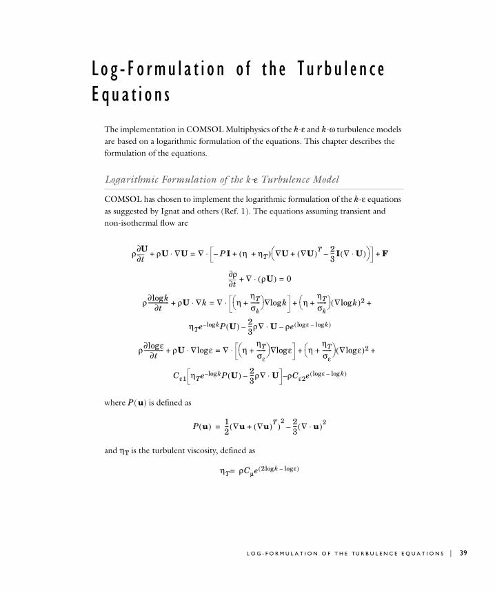
The implementation in COMSOL Multiphysics of the k-ε and k-ω turbulence models are based on a logarithmic formulation of the equations. This chapter describes the formulation of the equations.
Logarithmic Formulation of the k-ε Turbulence Model
COMSOL has chosen to implement the logarithmic formulation of the k-ε equations as suggested by Ignat and others (Ref. 1). The equations assuming transient and non-isothermal flow are
where P ( u) is defined as
and ηT is the turbulent viscosity, defined as
ρt∂
∂U ρU ∇U⋅+ ∇ P I– η ηT+( ) ∇U ∇U( )T 23---–+ I ∇ U⋅( )⎝ ⎠
⎛ ⎞+⋅ F+=
t∂∂ρ ∇+ ρU( )⋅ 0=
ρ∂ klog∂t
--------------- ρU ∇⋅+ k ∇ ηηT
σk-------+⎝ ⎠
⎛ ⎞ klog∇ ηηT
σk-------+⎝ ⎠
⎛ ⎞ ∇ klog( )2+ +⋅=
ηTe klog– P U( ) 23---ρ∇ U⋅– ρe εlog klog–( )–
ρ∂ εlog∂t
-------------- ρU ∇ εlog⋅+ ∇ ηηT
σε-------+⎝ ⎠
⎛ ⎞ εlog∇ ηηT
σε-------+⎝ ⎠
⎛ ⎞ ∇ εlog( )2+ +⋅=
Cε1 ηTe klog– P U( ) 23---ρ∇ U⋅– ρCε2e εlog klog–( )–
P u( ) 12--- ∇u ∇u( )T
+( )2 2
3--- ∇ u⋅( )2
–=
ηT ρCµe 2 k εlog–log( )=
L O G - F O R M U L A T I O N O F T H E TU R B U L E N C E E Q U A T I O N S | 39

40 | C H A P T E R
Logarithmic Formulation of the k-ω Turbulence Model
The equations for the k-ω turbulence model, assuming transient and non-isothermal flow, are
where P (u) is defined as
and ηT is the turbulent viscosity, defined as
Reference
1. L. Ignat, D. Pelletier, and F. Ilinca, “A universal formulation of two-equation models for adaptive computation of turbulent flows,” Computer methods in applied mechanics and engineering, vol. 189, pp. 1119–1139, 2000.
ρ∂ klog∂t
--------------- ρU ∇⋅+ k ∇ η σkηT+( ) klog∇[ ] η σkηT+( ) ∇ klog( )2+ +⋅=
ηTe klog– P U( ) 23---ρ∇ U⋅– βkρe ωlog–
ρ∂ ωlog∂t
---------------- ρU ∇ ωlog⋅+ ∇ η σωηT+( ) ωlog∇[ ] η σωηT+( ) ∇ ωlog( )2+ +⋅=
α ηTe klog– P U( ) 23---ρ∇ U⋅– ρβe ωlog–
P u( ) 12--- ∇u ∇u( )T
+( )2 2
3--- ∇ u⋅( )2
–=
ηT ρe klog ωlog–=
2 : A P P L I C A T I O N M O D E I M P L E M E N T A T I O N S

S p e c i a l E l emen t T y p e s F o r F l u i d F l ow
The list of predefined elements in the Incompressible Navier-Stokes application mode and its variants includes some special element types in addition to the standard Lagrange elements. These elements are potentially useful for applications in fluid dynamics and are listed in Ref. 1.
All these elements include bubble shape functions to approximate the velocity variables and/or discontinuous shape functions for approximating pressure. The table below provides a short description of these special elements.
The notation used for the element names is taken from Ref. 1 and summarized below:
• Pm Pn, where m > 0 and n > 0, denotes that the velocity variables are approximated by a polynomial shape function of order m and that the pressure is approximated by
TABLE 2-43: INCOMPRESSIBLE NAVIER-STOKES—SPECIAL ELEMENT TYPE
ELEMENT NAME 2D 3D DESCRIPTION
P1+ P1 (Mini) √ √ Similar to the Lagrange - Linear element with an
additional bubble shape function to approximate the velocity variables
P2 P0 √ The pressure is approximated by a discontinuous function which is piecewise constant (that is, of order 0) in each element and discontinuous on the element edges
P2+ P1 √ Similar to Lagrange - P2 P1 with an additional
bubble shape function to approximate the velocity variables. Considered to be a good element (Ref. 1)
P2 (P1+P0) √ √ Similar to Lagrange - P2 P1 with an additional discontinuous shape function to approximate the pressure
P2 P-1 √ Similar to Lagrange - P2 P1 with the exception that the pressure is described by a linear shape function which is discontinuous at the element edges. This element is pointwise divergence-free
P2+ P-1 (Crouzeix-Raviart) √ √ Similar to Lagrange - P2 P1 with an additional
bubble shape function to approximate the velocity variables and a linear shape function that is discontinuous on the element edges to approximate the pressure. Considered to be a good element (Ref. 1)
S P E C I A L E L E M E N T TY P E S F O R F L U I D F L O W | 41

42 | C H A P T E R
a polynomial shape function of order n. Both the velocity and the pressure variables are continuous on the element edges.
• Pm+ Pn is similar to the above with a bubble shape function added to approximate
the velocity variables. The bubble shape function is of order 3 in 2D (order 4 in 3D) and is zero on the element edges.
• Pm P−n, where m > 0 and n ≥ 0, is similar to the first case (Pm Pn) with the exception that the shape function for the pressure is discontinuous on the element edges.
• Pm (Pn + Pq) is also similar to the first case (Pm Pn) with an additional shape function added to approximate the pressure.
It is difficult to choose the optimal element for a specific model. The table above provides some brief characteristics on each element. Ref. 1 is recommended for further reading on these elements.
Exploring element-specific variables Some of the predefined elements introduce additional variables. For the elements that include a bubble shape function, the velocity is approximated by:
(2-2)
(2-3)
(2-4)
where ul, vl, and wl are contributions from the Lagrange shape functions, and ub, vb, and wb are contributions from the bubble shape functions. Each contribution can be plotted separately. For example, to plot the contribution from the bubble shape function to the velocity when using the Navier-Stokes application mode, plot the expression ub_chns.
Similarly, for the P2 (P1 + P0) element, the pressure is represented by:
(2-5)
You can plot each pressure contribution separately by using the expressions p1_chns and p2_chns, respectively, in the Incompressible Navier-Stokes application mode.
Values for integration and constraint order Each predefined element type has its own default values for integration order (gporder) and constraint order (cporder). For the bubble shape functions, the required integration order is relatively high. These elements in combination with a large and dense mesh can therefore lead to high
u ul ub+=
v vl vb+=
w wl wb+=
p p1 p2+=
2 : A P P L I C A T I O N M O D E I M P L E M E N T A T I O N S

memory consumption. For this reason, the default gporder value for the Crouzeix-Raviart element (P2 + P−1) in 3D is somewhat lower than what would be theoretically required. For the other element types that include bubble shape functions, you may have to reduce gporder manually by one or two units to reduce memory consumption.
Reference
1. P.M. Gresho and R.L. Sani, Incompressible Flow and the Finite Element Method, 2nd vol., John Wiley & Sons Ltd, 2000.
S P E C I A L E L E M E N T TY P E S F O R F L U I D F L O W | 43

44 | C H A P T E R
2 : A P P L I C A T I O N M O D E I M P L E M E N T A T I O N S
I N D E X
A application mode variables 7
application scalar variables 7
application variables 7
B bubble shape function 41
C Crouzeix-Raviart element 41
D dependent variables 7
discontinuous shape function 41
K k-epsilon turbulence mode
logarithmic formulation 39
k-omega turbulence mode
logarithmic formulation 40
M mobility 35, 37
N non-Newtonian viscosity 13
S shear rate 13
special element types
fluid flow 41
T typographical conventions 1
I N D E X | 45

46 | I N D E X