Letter of Transmittal

April 28, 2015

Dr. Jonathan Whitlow, Professor

Chemical Engineering Department

College of Engineering

Florida Institute of Technology

150 West University Blvd.

Melbourne, FL 32901

Dear Dr. Whitlow,

We have enclosed our report on the proposed bitumen hydrocarbon extraction and upgrading plant to convert bitumen in Athabasca, Canada to synthetic crude oil. The report details the preliminary design of the new plant including equipment sizes and costs, manufacturing costs, and an economic analysis. A sensitivity analysis is also included on the effect of methane and oil prices on the rate of return on investment.

If you have any questions or concerns, please contact Samantha McCuskey at smccuskey2011@my.fit.edu, Athela Frandsen at afrandsen2012@my.fit.edu, or Dennis Hogan at dhogan2012@my.fit.edu.

Sincerely,

Samantha McCuskey

Athela Frandsen

Dennis Hogan

2

Contents

Executive Summary ........................................................................................................................ 6

Introduction ..................................................................................................................................... 7

Process Description ......................................................................................................................... 9

Process Design and Simulation ..................................................................................................... 31

Gas Turbine and HRSG............................................................................................................. 32

Well ........................................................................................................................................... 32

Heat Exchangers ........................................................................................................................ 34

Splitters...................................................................................................................................... 34

Distillation Columns ................................................................................................................. 34

Reactors ..................................................................................................................................... 35

Pumps ........................................................................................................................................ 36

3-D Modeling ............................................................................................................................ 36

Capital Costs ................................................................................................................................. 38

Manufacturing Costs ..................................................................................................................... 43

Profitability and Sensitivity Analysis ........................................................................................... 47

Safety & Environmental ............................................................................................................... 54

Process Control ............................................................................................................................. 56

References ..................................................................................................................................... 61

Appendix A: All Equipment Design Methods, Calculations and Assumptions ........................... 70

Injection ..................................................................................................................................... 70

HRSG ........................................................................................................................................ 71

Darcy Theory ......................................................................................................................... 72

Settlers ....................................................................................................................................... 74

Distillation ................................................................................................................................. 75

Hydrocracker ............................................................................................................................. 77

Appendix B: Sample Calculations for Capital Cost ..................................................................... 83

Turbines/Compressors/Pumps/Salt Heaters: ............................................................................. 83

Reactors: .................................................................................................................................... 84

Towers: ...................................................................................................................................... 85

Heat Exchangers:....................................................................................................................... 87

3

Ferric Sulfate Cost ..................................................................................................................... 87

Appendix C: Sample Calculations for Manufacturing Cost ......................................................... 92

Refrigerated Water Cost ............................................................................................................ 92

Appendix D: Profitability Calculations ........................................................................................ 97

Appendix E: Literature Review .................................................................................................. 101

Separation Processes ............................................................................................................... 104

Catalyst Characteristics ........................................................................................................... 105

Reactor .................................................................................................................................... 107

Safety and Environmental Concerns ....................................................................................... 107

Appendix F: Project Timeline ..................................................................................................... 109

4

Figures

Figure 1: Bitumen SCO Production Predictions in Canada ............................................................ 8

Figure 2: PFD Section 1: Injection Fluid Generation and Initial Separation ................................ 13

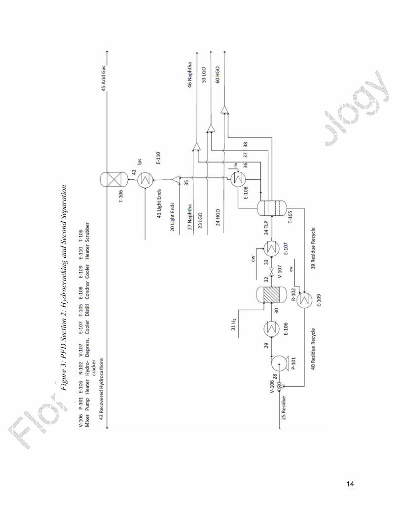
Figure 3: PFD Section 2: Hydrocracking and Second Separation ................................................ 14

Figure 4: PFD Section 3: Component Hydrotreatment and Final Product Blend......................... 15

Figure 5: General Hydrocracker Equations .................................................................................. 35

Figure 6: SolidWorks 3D Design .................................................................................................. 37

Figure 7: Capitol Costs ................................................................................................................. 38

Figure 8: Manufacturing Costs ..................................................................................................... 43

Figure 9: Profit Distribution.......................................................................................................... 47

Figure 10: Profitability Analysis ................................................................................................... 49

Figure 11: Effect of Varying Methane Price on Cumulative Profit .............................................. 50

Figure 12: Effect of Varying Oil Price on Cumulative Profit ....................................................... 51

Figure 13: Effect of Random Fluctuations in Oil Price on Cumulative Profit ............................. 52

Figure 14: P&ID Section 1: Injection Fluid Generation and Initial Separation ........................... 58

Figure 15: P&ID Section 2: Hydrocracking and Second Separation ............................................ 59

Figure 16: P&ID Section 3: Component Hydrotreatment and Final Product Blend .................... 60

Figure 17: HYSYS Injection Simulation ...................................................................................... 70

Figure 18: HYSYS HRSG Simulation .......................................................................................... 71

Figure 19: Darcy Theory ............................................................................................................... 72

Figure 20: HYSYS Settler Simulation .......................................................................................... 74

Figure 21: 1st Settler Components in HYSYS ............................................................................. 74

Figure 22: HYSYS Vacuum Distillation Column Simulation ...................................................... 75

Figure 23: Distillation Column Exit Stream Composition in HYSYS ......................................... 76

Figure 24: HYSYS Hydrocracker ................................................................................................. 77

Figure 25: Hydrocracker Black Boxing 1 ..................................................................................... 78

Figure 26: Hydrocracker Black Boxing 2 ..................................................................................... 79

Figure 27: HYSYS Hydrotreaters ................................................................................................. 80

Figure 28: Hydrotreaters Black Boxing 1 ..................................................................................... 81

Figure 29: Hydrotreaters Black Boxing 2 ..................................................................................... 81

Figure 30: Hydrotreaters Black Boxing 3 ..................................................................................... 82

5

Tables Table 1: Stream Information 1-24................................................................................................. 16

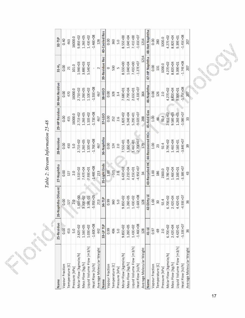
Table 2: Stream Information 25-48............................................................................................... 17

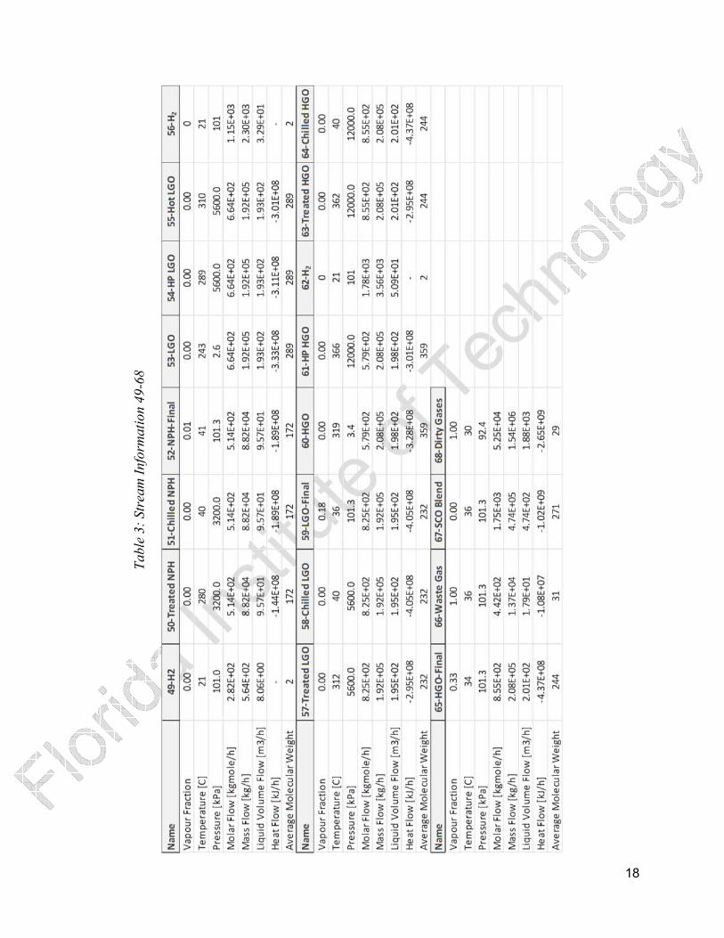
Table 3: Stream Information 49-68............................................................................................... 18

Table 4: Stream Compositions 1-8 ............................................................................................... 19

Table 5: Stream Compositions 9-16 ............................................................................................. 20

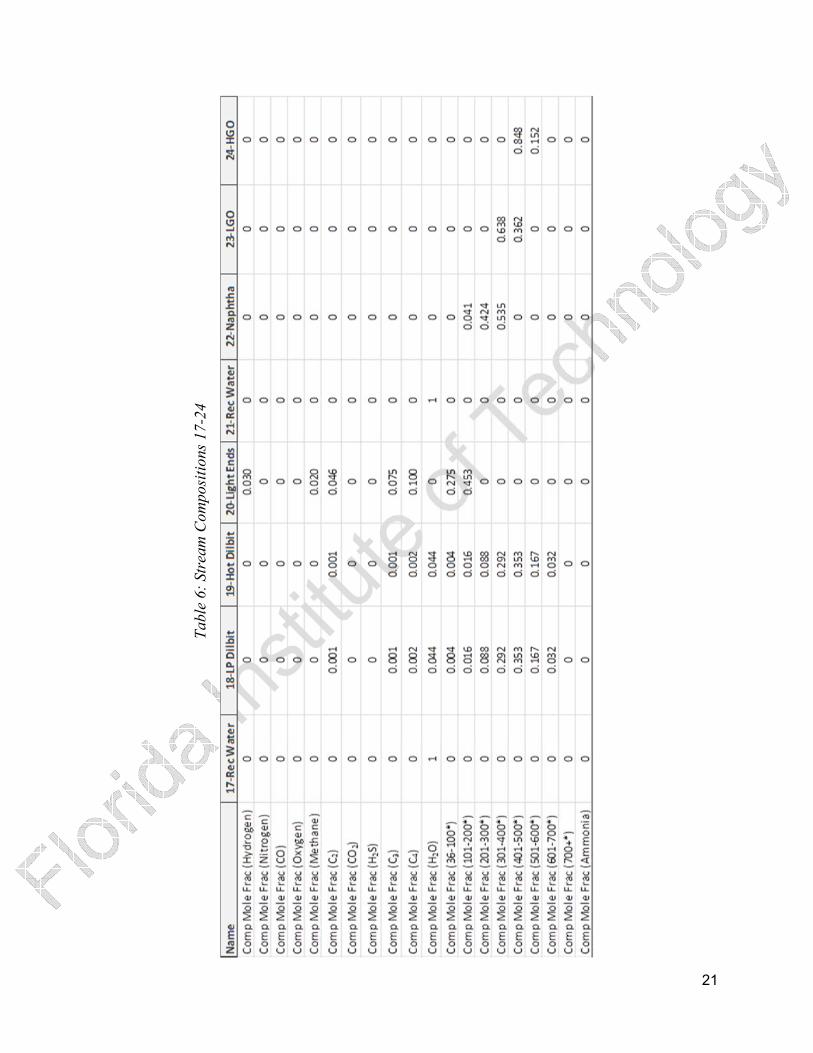
Table 6: Stream Compositions 17-24 ........................................................................................... 21

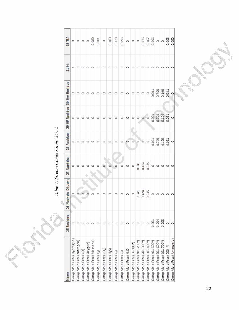
Table 7: Stream Compositions 25-32 ........................................................................................... 22

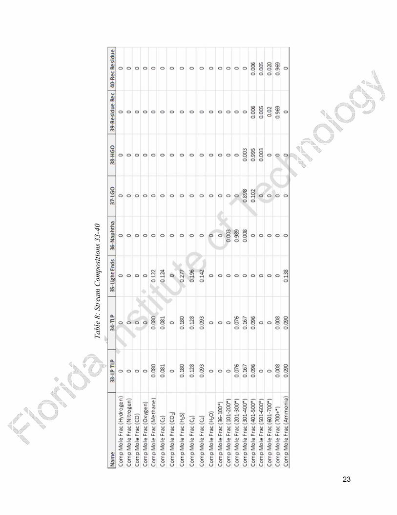
Table 8: Stream Compositions 33-40 ........................................................................................... 23

Table 9: Stream Compositions 41-48 ........................................................................................... 24

Table 10: Stream Compositions 49-56 ......................................................................................... 25

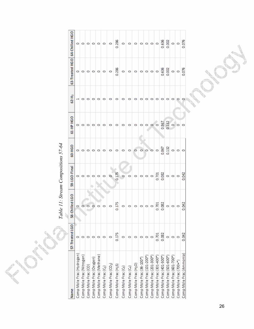
Table 11: Stream Compositions 57-64 ......................................................................................... 26

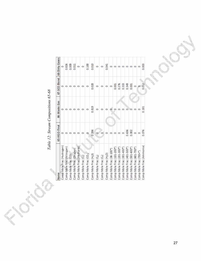
Table 12: Stream Compositions 65-68 ......................................................................................... 27

Table 13: Equipment Specifications: Reactors ............................................................................. 28

Table 14: Equipment Specifications: Compressors, Turbine, and Pumps .................................... 28

Table 15: Equipment Specifications: Electric Heaters ................................................................. 29

Table 16: Equipment Specifications: Towers ............................................................................... 29

Table 17: Utilities: Water .............................................................................................................. 30

Table 18: Utilities: Electricity Use ............................................................................................... 30

Table 19: Equipment Specifications: Heat Exchangers ................................................................ 30

Table 20: Capital Cost Summary .................................................................................................. 38

Table 21: Summary of Manufacturing Costs ................................................................................ 43

Table 22: Cumulative Profit Change from Change in Methane Price .......................................... 50

Table 23: Compressor Capital Costing ......................................................................................... 83

Table 24: Reactor Costing ............................................................................................................ 84

Table 25: Tower Costing .............................................................................................................. 86

Table 26: Packing Costing ............................................................................................................ 86

Table 27: Capital Costing Spreadsheet 1 ...................................................................................... 88

Table 28: Capital Costing Spreadsheet 2 ...................................................................................... 89

Table 29: Capital Costing Spreadsheet 3 ...................................................................................... 90

Table 30: SRU Costing ................................................................................................................. 91

Table 31: Manufacturing Cost Spreadsheet .................................................................................. 93

Table 32: Raw Materials and Cost of Labor ................................................................................. 94

Table 33: Cost of Utilities ............................................................................................................. 95

Table 34: Plant Sales Calculations ................................................................................................ 96

Table 35: Profitability Calculations 1 ........................................................................................... 97

Table 36: Profitability Calculations 2 ........................................................................................... 98

Table 37: Methane Sensitivity ...................................................................................................... 99

Table 38: Oil Price Sensitivity .................................................................................................... 100

Table 39: Overview of Bitumen Extraction Processes ............................................................... 102

6

Executive Summary

Synthetic crude oil (SCO) is produced after extracting and upgrading bitumen from a

well in Athabasca, Canada. An injection fluid of water is utilized to extract the bitumen from the

ground via Steam Assisted Gravity Drainage (SAGD). The upgrading is then completed in situ,

or on-site, rather than diluting the bitumen and pumping for off-site processing. Cokers have

been used to process bitumen, however with the addition of a catalyst such as ferric sulfate,

reactions can occur at lower temperatures. This reduces the cost of the reactors as well as

increases their safety. In addition, extensive modeling was done to calculate the pressure drop

through the well and to model the reactions in the hydrocracker and hydrotreaters.

The production rate was 71,500 bbl/day for 330 days of operation per year, resulting in

sales of over $1.5 Billion every year and a total cumulative profit of $6.9 billion at the end of the

12 year plant life. The plant was simulated in HYSYS and Aspen Plus V8.6 after an extensive

literature review to assess sizing of equipment. Total capital costs were $415.7 Million and

manufacturing costs were $368.7 million. The plant reached profitable status in approximately

2.3 years. The internal rate of return is 74.3% with an return on investment of 15.64. Profitability

was most impacted by reduction of synthetic crude oil price; however the plant was still

profitable after 12 years even if oil prices decreased 5% per year.

7

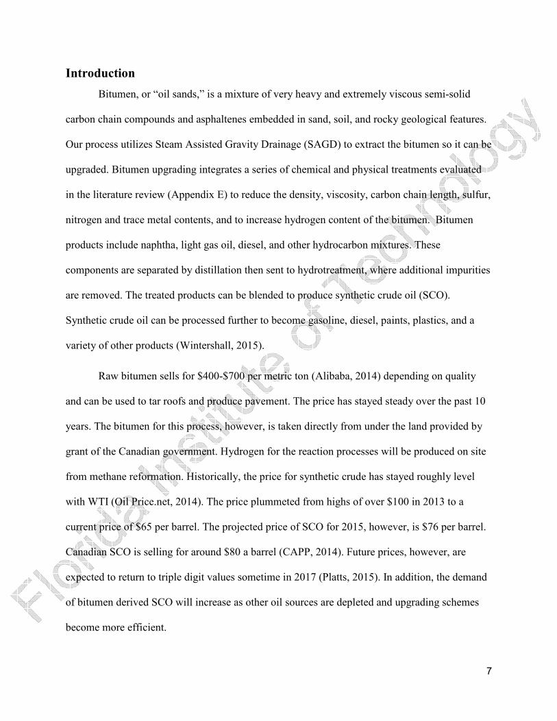
Introduction

Bitumen, or “oil sands,” is a mixture of very heavy and extremely viscous semi-solid

carbon chain compounds and asphaltenes embedded in sand, soil, and rocky geological features.

Our process utilizes Steam Assisted Gravity Drainage (SAGD) to extract the bitumen so it can be

upgraded. Bitumen upgrading integrates a series of chemical and physical treatments evaluated

in the literature review (Appendix E) to reduce the density, viscosity, carbon chain length, sulfur,

nitrogen and trace metal contents, and to increase hydrogen content of the bitumen. Bitumen

products include naphtha, light gas oil, diesel, and other hydrocarbon mixtures. These

components are separated by distillation then sent to hydrotreatment, where additional impurities

are removed. The treated products can be blended to produce synthetic crude oil (SCO).

Synthetic crude oil can be processed further to become gasoline, diesel, paints, plastics, and a

variety of other products (Wintershall, 2015).

Raw bitumen sells for $400-$700 per metric ton (Alibaba, 2014) depending on quality

and can be used to tar roofs and produce pavement. The price has stayed steady over the past 10

years. The bitumen for this process, however, is taken directly from under the land provided by

grant of the Canadian government. Hydrogen for the reaction processes will be produced on site

from methane reformation. Historically, the price for synthetic crude has stayed roughly level

with WTI (Oil Price.net, 2014). The price plummeted from highs of over $100 in 2013 to a

current price of $65 per barrel. The projected price of SCO for 2015, however, is $76 per barrel.

Canadian SCO is selling for around $80 a barrel (CAPP, 2014). Future prices, however, are

expected to return to triple digit values sometime in 2017 (Platts, 2015). In addition, the demand

of bitumen derived SCO will increase as other oil sources are depleted and upgrading schemes

become more efficient.

8

Figure 1: Bitumen SCO Production Predictions in Canada

The production of Canadian bitumen is expected to increase significantly, as seen in

Figure 1 (Munteanu, 2012). The daily production rate for our design is 71,500 bbl/day of SCO

with the annual production rate totaling to 23.6 million barrels. The plant upgrades the bitumen

on-site in Athabasca, Canada. One significant benefit of this is to reduce the difficulty of

cleaning up spills during transport. This is a result of SCO’s lower density, allowing for spilled

material to float whereas raw bitumen would sink (Song, 2012). The plant also utilizes newer

hydrocracker technology, reactors which achieve higher conversions of feed with lower

temperatures through the use of a catalyst (see price calculations in Appendix B) versus older

coking methods; which not only require more energy to operate, but also create undesired

byproducts of coke and ash. The plant design also includes consideration for carbon dioxide

sequestration, an installed sulfur recovery unit, and an ammonia scrubber.

0.0

1.0

2.0

3.0

4.0

5.0

6.0

2010 2012 2014 2016 2018 2020 2022 2024 2026 2028 2030 2032

MB

PD

(M

illi

on

Barr

els

Per

Day)

Year

Canadian Bitumen Production Projection

9

Process Description

The overall process includes generation of the injection fluid, initial separation of the

bitumen feed out of the well into components, hydroconversion of the heaviest component,

further separation into parts, hydrotreatment of combined cuts, and finally blending of the SCO

product. Figures 2-4 show the process flow diagram and Tables 1-3 show stream properties

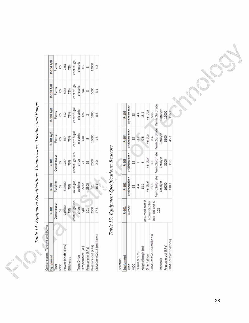
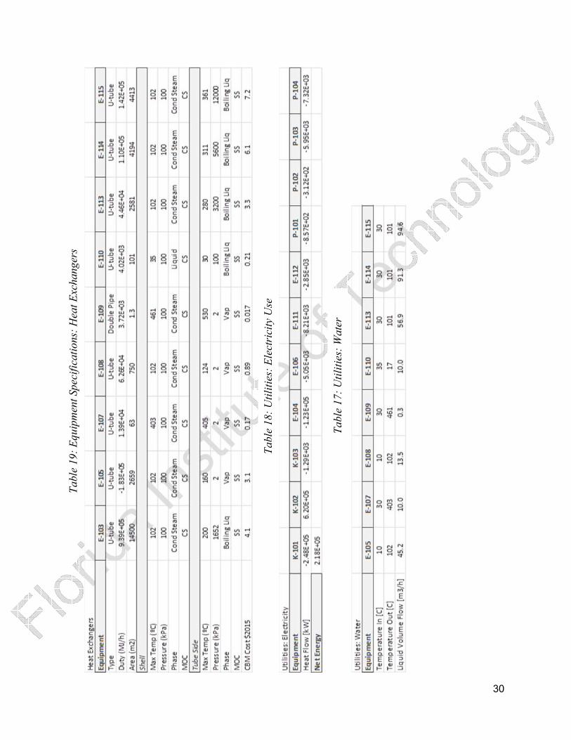
while Tables 4-12 detail compositions. Finally, Tables 13-16 and 19 describe the equipment

sizes and materials of construction. Tables 17 and 18 show utilities.

Figure 2 shows the injection process and initial separation of the well feed. Compressed

air, fuel and recovered hydrocarbons from downstream (streams 1, 3, and 43) are compressed

and sent to a gas turbine. The gas turbine is comprised of compressors (K-101 and K-103), a

burner (R-101), and an expander (K-102). Low pressure combustion gas (stream 5) is sent to a

Heat Recovery Steam Generator, which is approximated as a cooler and heater that work in

tandem. The cooler (E-101) cools the combustion gas and sends it to a tower (T-101) where the

condensate water is separated from the exhaust. Water from the tower and process recycle

streams (stream 9) is turned to steam in the heater (E-102), which receives its energy from the

cooler. The fluid (stream 10) is injected into the well at 240 C and 2500 kPa.

In the well, the steam causes a separation of the bitumen from the geological formations

by reducing its viscosity. The water/bitumen mixture then drains to the production pipe and

transported up to the production facility by the residual pressure in the well.

The well feed (stream 11) is a mixture of bitumen, water and sand at 200 C and 1600 kPa.

The feed is cooled by exchanging heat (E-103) to a recycled water stream (stream 15) that is

being sent back to the injection process. The cooled feed is separated in the first settling tank (T-

102) whose primary purpose is to remove the sand and a majority of water from the stream. The

10

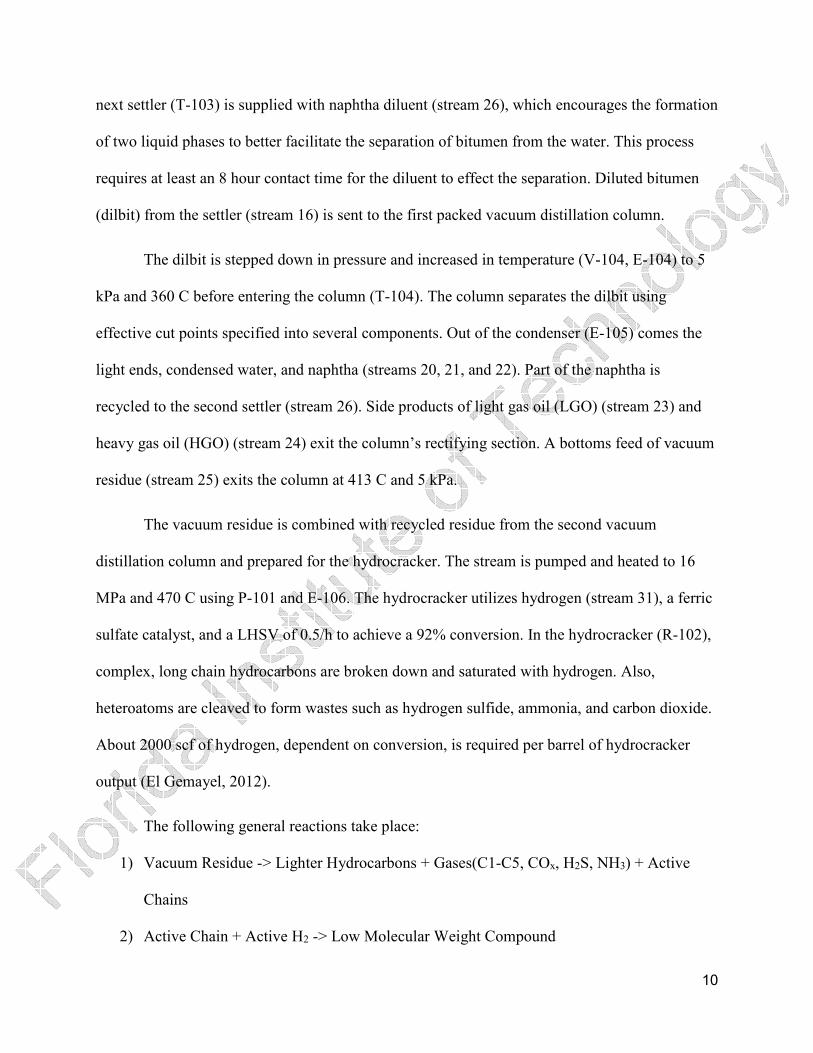
next settler (T-103) is supplied with naphtha diluent (stream 26), which encourages the formation

of two liquid phases to better facilitate the separation of bitumen from the water. This process

requires at least an 8 hour contact time for the diluent to effect the separation. Diluted bitumen

(dilbit) from the settler (stream 16) is sent to the first packed vacuum distillation column.

The dilbit is stepped down in pressure and increased in temperature (V-104, E-104) to 5

kPa and 360 C before entering the column (T-104). The column separates the dilbit using

effective cut points specified into several components. Out of the condenser (E-105) comes the

light ends, condensed water, and naphtha (streams 20, 21, and 22). Part of the naphtha is

recycled to the second settler (stream 26). Side products of light gas oil (LGO) (stream 23) and

heavy gas oil (HGO) (stream 24) exit the column’s rectifying section. A bottoms feed of vacuum

residue (stream 25) exits the column at 413 C and 5 kPa.

The vacuum residue is combined with recycled residue from the second vacuum

distillation column and prepared for the hydrocracker. The stream is pumped and heated to 16

MPa and 470 C using P-101 and E-106. The hydrocracker utilizes hydrogen (stream 31), a ferric

sulfate catalyst, and a LHSV of 0.5/h to achieve a 92% conversion. In the hydrocracker (R-102),

complex, long chain hydrocarbons are broken down and saturated with hydrogen. Also,

heteroatoms are cleaved to form wastes such as hydrogen sulfide, ammonia, and carbon dioxide.

About 2000 scf of hydrogen, dependent on conversion, is required per barrel of hydrocracker

output (El Gemayel, 2012).

The following general reactions take place:

1) Vacuum Residue -> Lighter Hydrocarbons + Gases(C1-C5, COx, H2S, NH3) + Active

Chains

2) Active Chain + Active H2 -> Low Molecular Weight Compound

11

3) Active Chain + Active Chain -> High Molecular Weight Compound

The output of treated liquid product (TLP) (stream 32) is prepared for the second packed

vacuum distillation column via a valve and cooler (V-107, E-107) to 360 C and 5 kPa. This

column (T-105) has similar outputs as the first column. These outputs include light ends,

naphtha, LGO, HGO, and vacuum residue (streams 35-39). The vacuum residue is cooled (E-

109) and recycled to the hydrocracker. The other streams are combined with their respective cuts

from the first distillation column.

The combined light ends (stream 41) are heated (E-110) with low pressure steam before

being scrubbed (T-106). The scrubber splits the hydrocarbons from the wastes of H2S, NH3 and

CO2. The recovered hydrocarbons are recycled back to the injection process (stream 43) where

they are compressed and burned in the gas turbine.

The combined naphtha, LGO and HGO streams are individually heated and pressurized

to prepare them for hydrotreatment. Each hydrotreater uses the ferric sulfate catalyst and

hydrogen to achieve further upgrading of the hydrocarbons by cleaving heteroatoms. The

naphtha (stream 46) is pumped and heated (P-102, E-111) to 280 C and 3200 kPa to prepare it

for hydrotreatment (R-103). Hydrotreatment of the naphtha requires a LHSV of 5/h and about

400 scf of hydrogen per barrel produced.

The LGO (stream 53) is pumped and heated to 310 C and 5600 kPa for hydrotreatment

(R-104). The LGO hydrotreater requires a LHSV of 2.5/h and 800 scf of hydrogen per barrel of

production. The HGO (stream 60) is pumped to 366 C and 12 MPa for hydrotreatment (R-105).

The HGO hydrotreater requires a LHSV of 1/h and 1200 scf of hydrogen per barrel of

production.

12

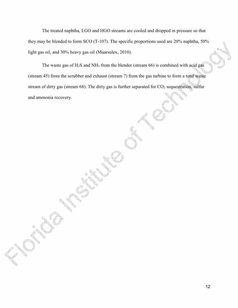
The treated naphtha, LGO and HGO streams are cooled and dropped in pressure so that

they may be blended to form SCO (T-107). The specific proportions used are 20% naphtha, 50%

light gas oil, and 30% heavy gas oil (Muarsulex, 2010).

The waste gas of H2S and NH3 from the blender (stream 66) is combined with acid gas

(stream 45) from the scrubber and exhaust (stream 7) from the gas turbine to form a total waste

stream of dirty gas (stream 68). The dirty gas is further separated for CO2 sequestration, sulfur

and ammonia recovery.

13

Fig

ure

2:

PF

D S

ecti

on 1

: In

ject

ion F

luid

Gen

erati

on a

nd I

nit

ial

Sep

ara

tion

14

Fig

ure

3:

PF

D S

ecti

on 2

: H

ydro

cra

ckin

g a

nd S

econd S

epara

tion

15

Fig

ure

4:

PF

D S

ecti

on 3

: C

om

ponen

t H

ydro

trea

tmen

t and F

inal

Pro

duct

Ble

nd

16

Table

1:

Str

eam

Info

rmati

on 1

-24

17

Table

2:

Str

eam

Info

rmati

on 2

5-4

8

18

Table

3:

Str

eam

Info

rmati

on 4

9-6

8

19

Table

4:

Str

eam

Com

posi

tions

1-8

20

Table

5:

Str

eam

Com

posi

tions

9-1

6

21

Table

6:

Str

eam

Com

posi

tions

17-2

4

22

Table

7:

Str

eam

Com

posi

tions

25-3

2

23

Table

8:

Str

eam

Com

posi

tions

33-4

0

24

Table

9:

Str

eam

Com

posi

tions

41-4

8

25

Table

10:

Str

eam

Com

posi

tions

49-5

6

26

Table

11:

Str

eam

Com

posi

tions

57-6

4

27

Table

12:

Str

eam

Com

posi

tions

65-6

8

28

Table

14:

Equip

men

t Sp

ecif

icati

ons:

Com

pre

ssors

, T

urb

ine,

and P

um

ps

Table

13:

Equip

men

t Sp

ecif

icati

ons:

Rea

ctors

29

Table

16:

Equip

men

t Sp

ecif

icati

ons:

Tow

ers

Table

15:

Equip

men

t Sp

ecif

icati

ons:

Ele

ctri

c H

eate

rs

30

Table

19:

Equip

men

t Sp

ecif

icati

ons:

Hea

t E

xchan

ger

s

Table

18:

Uti

liti

es:

Ele

ctri

city

Use

Table

17:

Uti

liti

es:

Wate

r

31

Process Design and Simulation

Aspentech’s HYSYS v8.6 was chosen for the majority of our process modeling. While

we initially were considering Aspentech’s Aspen Plus v8.6 to conduct our modeling, we

immediately discovered Aspen Plus’ inability to easily address complex mixtures like raw

petroleum, comprised of thousands of components. After initial failures at simplifying the

characterization of bitumen in order to enable Aspen Plus, it was abandoned in favor of HYSYS;

a software package new to us, requiring additional study and training to use effectively.

Several weeks were spent exploring and consuming freely available online training

manuals, particularly those from Colorado School of Mines and the University of Alberta. With

enough background, we began simulation using a petroleum assay preloaded into Aspen

HYSYS’s database, Athabasca 2006. We characterized the assay using the automated assay

characterization function provided by Aspen HYSYS’ “Oil Manager” interface. This

characterized the assay into several dozen hypothetical groups (cuts) separated by their boiling

points, each cut being in a ten degree range. HYSYS treats each cut as an individual molecule

for simulation purposes. While the default is ten degrees, high accuracy of modeling could be

achieved by lowering the cut range. We chose to continue with default settings. The assay was

taken from a bitumen deposit located in the Athabasca region, and using this assay we chose to

locate the plant in Athabasca, Canada.

The Peng-Robinson equation of state was utilized for the HYSYS simulation (Peng &

Robinson, 1976). Not only is Peng-Robinson recommended by Aspentech for use of processing

heavy oils in HYSYS, but Peng-Robinson was also developed for the purpose of correcting the

failings other equations of state have with handling high viscosity fluids of high molecular

weight (AspenTech, 2010). No assumptions were necessary to accomplish this given that our

32

feeds was automatically characterized from a pre-loaded petroleum assay (Athabasca 2006)

found in the HYSYS assay database. Each unit operation required in the plant was simulated in

HYSYS or black boxed in Excel. Further details of these designs are shown in Appendix A and

C.

Gas Turbine and HRSG

The first section of the plant involves a gas turbine and heat recovery steam generator

(HRSG) to generate the injection fluid and electricity to power other unit operations and plant

utilities. These were simulated as multiple blocks. The gas turbine was broken down as a

compressor for the air and fuel intake, a Gibbs reactor to represent the burner, and an expander to

represent the exhaust output. The Gibbs reactor was selected for convenience, as the unit

operation in HYSYS was preloaded with a database of combustion reactions. As such, the Gibbs

reactor can function without specifying reaction stoichiometry.

Next the HRSG is simulated as cooler and heater blocks that operate congruently. The

cooler removes heat from the gas turbine’s combustion gas. The combustion gas is then

separated into water and exhaust. The condensed water as well as recycled process water is

passed through the heater block which derives its power directly from the cooler block. The

heater changes the water to steam for the injection process. With this design, tuning the injection

fluid to the properties necessary would be conducted at the gas turbine, varying mass flow of fuel

and air.

Well

In HYSYS, the well is represented as a Petroleum Feeder block. The feeder effectively

“feeds” results from a characterized petroleum assay into an influent feed stream, such that the

effluent stream carries that assay’s components combined with the influent at a ratio specified by

33

the user. In our case, bitumen, water and sand exit the well. Since HYSYS cannot simulate sand,

and it is easily removed due to its specific gravity, it was neglected in the simulation. With our

injection steam made the influent to the feeder, a volume ratio of 75% water was decided to

represent the output characteristics of a developed well based on data provided by the University

of Alberta (NSERC 2015).

The pressure drop through the well was modeled using Darcy theory (Elliot 2001).

Assuming a Darcy travel time ratio of 0.8 (the ratio of time to travel the maximum vertical

distance in a bed to the time to travel the maximum horizontal distance in a bed by a hypothetical

Darcy particle) to represent a mostly developed well, the pressure drop was calculated to be 850

kPa. Subtracting this from the injection pressure, the pressure of the bitumen/water feed was

needed to exit the well in HYSYS at 1600 kPa. The pressure of the well output could not be

directly specified, so to achieve 1600 kPa, the vapor fraction was assumed to be zero and the

temperature was varied until the correct pressure was reached. This represents heat being

absorbed into the bitumen and the surrounding earth in the well. A “developed” well implies that

sufficient heat and pressure has already been applied such that the substrate of the well has been

broken up and fluidized. Further information regarding the Darcy based modeling and well

development has been included Appendix A.

Traditionally oil refining involves an initial process of desalting where water or other

polar solvents are added to the mixture to extract naturally occurring salts from the petroleum

mixture. As a result of the SAGD process, utilizing water already, salts are automatically

removed as part of the extraction process (El Gemayel, 2012). This was not included in the

model, as treatment of this salt-laden wastewater would necessitate an additional section of the

plant devoted to it and would likely tie into the already neglected brackish water treatment

34

system. This would also have produced salt waste, which was neglected as well. Typically 97-

99% of the produced water and brackish makeup water can be recovered through wastewater

treatment (Ondrey, 2012). However, as stated before, water treatment was outside of the scope of

this project.

Heat Exchangers

E-103 is the only heater simulated as a heat exchanger in HYSYS. Because it exchanges

heat between the hot bitumen/water feed and the recycled process water, it is embedded in the

SAGD process. All other heaters operate using arbitrary energy streams. As we were unable to

gather accurate sizing information from HYSYS for cost purposes, all exchangers were

replicated in Aspen using representative compounds with similar chemical properties at identical

stream conditions.

Splitters

Settler T-102, Settler T-103, and Scrubber T-106 were modeled using splitter blocks for

the convenience of specifying the split of components. This allowed complete separation that

cannot always be achieved under real conditions, as well as mitigating ignorance the team still

had using some of the unit operations offered by HYSYS. The costing of these units was

completed based on residence times determined by literature applied to process flow rates.

Distillation Columns

The two vacuum distillation columns, T-104 and T-105, were simulated using Petroleum

Distillation blocks. The block requires inputs of number of stages, feed stage, side product

stream stages, and effective cut points (ECPs) of the products. The ECPs are temperature cut-offs

that determine the composition range of the product streams from the column. These

temperatures were specified based on information from Leffler’s Petroleum Refining in

35

Nontechnical Language (2008). For sizing, the column was recreated in Aspen using specific

composition fractions mentioned in Appendix B. The packing resulting in the smallest diameter

was chosen, given that most diameter outputs were greater than 12m and therefore unrealistic.

This chosen packing was P90X Super-Pak Raschig metal packing.

Reactors

The hydrocracker was initially simulated in HYSYS using a Hydrocracker block but did

not function because of the wide range of molecular weights in the feed stream. The reactor for

hydroconversion in HYSYS, while capable of simulating cracking reactions, was not

programmed to simulate those reactions over the wide variety of components held by our

vacuum residue. Therefore, the hydrocracker was black boxed in Excel using reaction and

conversion equations from El Gemayel (2012). More detailed calculations are shown in

Appendix A as well as the spreadsheet labeled “Hydrocracker”.

Figure 5: General Hydrocracker Equations

To input the results into HYSYS a Petroleum Shift Reactor block was used. The Shift

Reactor allows arbitrary specification of the conversion of feed into a user specified set of

component streams. In our case these streams included hydrogen sulfide, ammonia, C1 through

C4 volatiles, naphtha, LGO, HGO, and unreacted residue. Since H2S and NH3 streams were

specified, these components needed to be manually removed from the assay to simulate that

heteroatoms were cleaved from the hydrocarbon molecules. This was achieved using a

Manipulator block, which allows for user editing of assay data at that point in the process. All

36

product streams from the petroleum shift reactor block and the assay manipulator block were

then recombined into one stream as the output of the hydrocracker, labeled as Treated Liquid

Product. The hydrotreaters were simulated in a similar way through Excel black boxing and the

Petroleum Shift Reactor block.

The final sulfur content of the SCO was found to be 0.03%, much lower than the

expected 0.13% (Muarsulex, 2010). This was likely due to the simulations being more ideal than

would occur in actual processes. In addition, when the hydrotreaters were being modeled in

Excel the sulfur content of various cuts were taken as averages instead of weighted averages.

This was done since the amount of time it would have taken to do a weighted average of sulfur

content for each cut (having a considerable number of cuts) would have been a prohibitive time

investment in order to ensure deadlines were met.

Pumps

Pumps added to the process were done so to effect necessary pressure changes at their

location. HYSYS was capable of simulating their use and no additional consideration was made

to their design.

3-D Modeling

The structure of the plant was also simulated using SolidWorks 2014 x64 edition.

Reference photos were used for various process equipment including the burner (Indeck, 2013),

HRSG (Kawasaki, 2014), heat exchangers (Bowman, 2015), settlers (White, 2012), pumps

(Kable, 2015), distillation columns (Vega, 2003), hydrocracker & hydrotreaters (Livingston,

2011), etc.

37

Figure 6: SolidWorks 3D Design

38

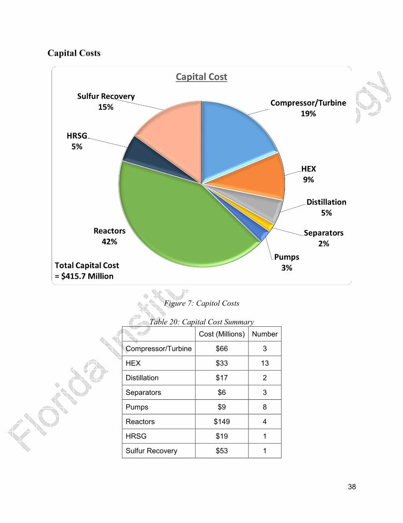
Capital Costs

Figure 7: Capitol Costs

Table 20: Capital Cost Summary

Cost (Millions) Number

Compressor/Turbine $66 3

HEX $33 13

Distillation $17 2

Separators $6 3

Pumps $9 8

Reactors $149 4

HRSG $19 1

Sulfur Recovery $53 1

39

The costing of the plant equipment follows a program set out in Turton’s Appendix A

(2008) based on the module factor approach to costing that was originally introduced by Guthrie

and modified by Ulrich. The costing program outputs equipment costs in 2001 dollars.

Bare Module Cost, CBM, of each piece of equipment is estimated by adding additional

costs associated with the equipment.

��� = ������ = ���( + �����) Additional costs (labor, piping, instrumentation, foundations, electrical, etc.) are tied up

into constants B1 & B2 given in Turton for heat exchangers, pumps & vessels.

Each piece of equipment is sized at standard conditions to determine the approximate

cost, Cp0.

log� ��� = � + �� log� � + ��(log��) 2 where A is the capacity or size parameter for the equipment, K1, K2 and K3 are given in Turton

for various types of equipment. The cost per unit of capacity decreases as the size of the

equipment increases. Each set of K values is only valid if the piece of equipment falls within the

size range given, or else the equipment must be scaled.

The materials factor, FM, is found using figures in Turton with the appropriate

identification number listed in tables. The materials factor is used for heat exchangers, process

vessels and pumps to account for materials of construction different than standard.

The pressure factor, FP, accounts for pressures other than atmospheric.

log� �� = � + �� log� � + ��(log��) 2

40

C1, C2 and C3 are given in Turton for various types of equipment, and P represents the pressure

in barg.

For vessels and towers, FP is calculated using the pressure and diameter, D.

��,������ =(� + 1)�2[850 − 0.6(� + 1)] + 0.00315

0.0063

For equipment operating at pressures less than -0.5 barg, FP,vessel is equal to 1.25.

For equipment that fell outside the capacity range given in Turton, a scaling equation was

used to find the cost of the new equipment. Where C is capacity, A is cost, and n is a cost

exponent.

�'�( = )�'�(*+

The burner R-101 is part of a gas turbine. Its cost is assumed to be included in the cost of

the compressor and turbine K-101 and K-102. The hydrocracker and hydrotreaters were cost as

towers, because of the high pressure and high capacities required. Each reactor volume was

found using the volumetric flow rate in and the LHSV given by El Gemayel (2012) and Speight

(2007).

It is assumed that the cost of drilling and preparing the well is negligible. The time taken

to develop the well is taken during the plant construction period (the first 2 years). Other specific

assumptions for other unit operations are listed in the sample calculations of Appendix B.

The costs were updated from $2001 to $2015 using a ratio of the CEPCI numbers. The

CEPCI from September 2001 is 397 and the CEPCI for 2015 as 610.

41

�,-. 2015 = �,-. 2001 ∗ (��0��1 2015�0��1 2001 )

Affixing a cost to the sulfur recovery module of the plant was done in far less standard

terms. Using SUPERCLAUS® process stoichiometry (Koscielnuk, D. et. al., 2015), it was

found that the sulfur recovery unit should be producing approximately 416 tonnes of elemental

sulfur per day, given hydrogen sulfide production from the reactor outputs. As a preliminary

design, the team saw fit to devise a simple scheme by which to assign this capital cost. Using

estimated module cost data provided by The European IPPC Bureau (Barthe, P., et. al. 2015), a

function was derived to relate sulfur production in tonnes per day, p, to total installed module

cost in millions of EUR, C.

� = 0.88882�.334�

Using the function, this plant’s value of 416 tonnes sulfur per day would effectively price the

sulfur recovery unit at $53M after conversion from 2015 Euros.

The upgrading process uses a catalyst, ferric sulfate, which is periodically regenerated.

The catalyst is considered a capital investment. It is assumed that the volume of catalyst needed

derived from the combined volume of reactors R-102, R-103, R-104, and R-105 minus a

recommended bed void fraction of 0.37 (Munteanu, 2012). Using the known density of the

catalyst, a total mass required was found. The catalyst cost is found from Alibaba of

$0.136/pound (Alibaba, 2015). The final catalyst cost is $290,627.81, negligible when compared

to the final capital cost.

The total module cost, CTM, (also known as the fixed capital investment, FCI) is found

by multiplying the bare module cost by 1.18. The 18% accounts for contingency and fee costs.

42

The total module cost for the Bitumen Extraction and Upgrading Plant is $415.7M. The capital

cost per barrel SCO in the first year produced is $17.61. Further information can be found on the

accompanying spreadsheet on the “Costing” tab.

43

Manufacturing Costs

Figure 8: Manufacturing Costs

Table 21: Summary of Manufacturing Costs

Fixed Capital Investment FCI $415.7M

Cost of Raw Materials CRM $194.9M

Cost of Waste Treatment CWT $41.4M

Cost of Utilities CUT $100

Cost of Labor COL $2.5M

The cost of manufacturing (COM) is based on the fixed capital investment (FCI), cost of

operating labor (COL), cost of utilities (CUT), cost of waste treatment (CWT), and cost of raw

materials (CRM) (Turton, 2008).

44

�56 = 0.18��1 + 2.73�58 + 1.23(�9: + �;: + �<6) The cost of labor (COL) is determined from the number of operators needed per shift and

their estimated salary. The number of operators per shift depends on the number of steps, P,

involving particulate solids handling and the number of steps not involving particulate solids

handling, Nnp. At the settling stage of the plant, sand must be removed from the process, so P=1.

The Nnp for the extraction and upgrading plant is found to be 25 and for the sulfur recovery unit

(SRU) is 6.

=>? = @(6.29 + 31.7�� + 0.23=+B) Labor for the main facility and the SRU has been calculated separately, as they should

have a significantly different set of daily tasks from one another. In the main unit, the number of

operators needed per shift is found to be 7. Assuming 4.5 shirts are required for each operator

needed, and there are no part-timers, a total of 32 operators will work at the main unit, which

operates 7920 hours of the year. Given a median salary for chemical engineers in the region of

Athabasca, Canada of C$69,891 (Payscale, 2015) the cost of labor is $1.8M per year after

conversion to USD. In the SRU, the number of operators needed per shift is found to be 2.8.

Assuming 4 operators are hired for each operator needed, and there are no part-timers, a total of

13 operators will work at the SRU, which also operates 7920 hours of the year. The cost of labor

for the SRU is then found to be $735,952.23 per year after conversion to USD.

The cost of utilities (CUT) is almost zero, but what there is comes from Turton to costs

the refrigerated water used in exchangers E-105 and E-108. The cost of the refrigerated water

totals out at $100.39/year. It is understood this cost does not account for the installation of

refrigeration units, which likely would be negligible against the total capital costs. Additional

45

cooling water is assumed to be drawn from brackish/saline aquifers in the immediate vicinity of

the facility. Canadian (and specifically Alberta) law has no regulations or license requirements

regarding the use of such aquifers, allowing the assumption of zero cost for their use (Griffiths,

2006). Any cost that would be incurred would be related to the purification of this source to

process quality, which has been neglected by the design team. The amount of electricity needed

for plant operation comes from the power generated by the gas turbine running off of recovered

hydrocarbons and natural gas. Electricity not used by the plant is assumed to be sold off to the

local grid at a price of 4 cents/kWh (Just Energy, 2014) and assumed as profit.

The cost of waste treatment (CWT) includes sequestration of carbon dioxide and SRU

operation. The recovery of ammonia to sellable product was assumed as an output from

scrubbing and not accurately modeled. Operation of the SRU was priced from published data

relating operating cost per day of particularly sized SRUs (Koscielnuk, D. et. al.). Knowing the

size of our SRU, a simple relation was made to assign an operating cost of the SRU as $3M/year.

Sequestration of carbon dioxide was priced at $21/tonne. This cost represents the operation of an

appropriately sized sequestration operation (Herzog, H., 2015). Capital costing of such a module

was neglected on the presumption this operation could be contracted out. Given the production

of 230.4 tonnes CO2 per hour, yearly sequestration costs are $38.3M. Combining these costs

brings a total CWT of $41.4M.

The cost of raw materials (CRM) is entirely derived from the price of natural gas. The

cost of natural gas in the region is provided on an energy basis at $4/Gigajoule (Just Energy,

2014). Through simulation it was found the plant would require 111,100 standard cubic meters

of methane directly to the gas turbine per hour to operate. A direct conversion relates one

gigajoule to 26.137 standard cubic meters (British Columbia Ministry of Finance, 2013). This

46

relationship allows for simple calculation of cost for methane consumed. Consumption of

methane by the gas turbine is calculated to cost $134.7M/year. While our process uses both

natural gas (methane) and hydrogen gas, it can be assumed hydrogen gas could be produced by

means of methane reformation, which relates the price of hydrogen to natural gas through

stoichiometry; a 4:10 molar ratio methane to hydrogen gas. Calculating CRM in this manner

neglects the cost of an installed reformation facility, and also neglects the production of

additional CO2. The design team decided this omission was acceptable given the scale of costs in

relation to larger costs.

The total cost of manufacturing is $415.7M in $2015. The breakdown of the costs can be

found in Figure 8 and Table 21. For manufacturing cost, $15.57 was found to be the cost/bbl

SCO produced. In addition, further information can be found on the accompanying spreadsheet

on the “Manufacturing” tab.

47

Profitability and Sensitivity Analysis

Figure 9: Profit Distribution

The products of the overall plant design include synthetic crude oil, elemental sulfur,

ammonia, and electricity. The annual sales for producing 71,530 barrels per day of SCO

assuming a price of $65/bbl is $1.53B. This is 92% of the total annual sales of $1.67B.

The annual sale for the sulfur output of 137,280 tonnes per year, assuming $400 per

tonne (Alibaba 2015), is $54.9M. This represents 3% of the total annual sales.

The ammonia recovered at 23,113 tonnes per year, priced at $400 per tonne assuming a

higher purity industrial grade mixture (Alibaba, 2015), yielded $9.3M annual profit. This

represents a very small fraction of the overall annual sales - only 0.6%.

48

After energy accounting, which can be seen in Appendix C, the plant produces a net 217

MW or 1.72E9 kWh/year. Electricity rates in Canada range from $0.03 to $0.12 per kWh.

Assuming a sell-back price of $0.04/kWh (Just Energy, 2014) results in an annual sale of

$68.8M. This represents 4% of the total annual sales, second after SCO sales.

The plant is sited in Athabasca, Canada, where the land needed is given by a land grant.

Investors are willing to give $200M in initial support. The working capital is 15% of the FCI at

$62.4M. It is assumed that the construction period for the plant is two years and the plant life is

10 years with no salvage. Straight line depreciation occurs at 10% per year. The tax rate is 25%.

It is assumed that both revenue and operating costs increase at a rate of 3% a year with a required

rate of return of 20%.

The annual distributed cash flow is the revenue minus the operating cost minus the taxes.

The present worth discrete cash flow is found using the monthly distributed cash flow, year of

the project, and monthly interest rate. The future worth discrete cash flow is the product of the

present worth and one plus the monthly interest rate raised to the total number of months. Finally

the net present and future worth are compounded to show the breakeven point.

The breakeven point is the time required for cumulative cash flow to equal zero. The

breakeven point of the plant occurs between the second and third year, approximated as 2.3

years. The internal rate of return is 74.3%. The calculations can be seen in Appendix D, and in

greater detail in the accompanying spreadsheet on the “Profitability” tab.

49

Figure 10: Profitability Analysis

A sensitivity analysis was performed on the cost of methane and SCO. The cost of

methane is influential on profitability due to its prominence in the manufacturing costs - about

64%. It can be assumed that the price of methane also affects the price of hydrogen, given that

the hydrogen was cost through methane reformation. Increasing methane costs by 10% every

year results in an overall COM increase of 6.5% a year. Figure 11 shows the new profitability

analysis.

50

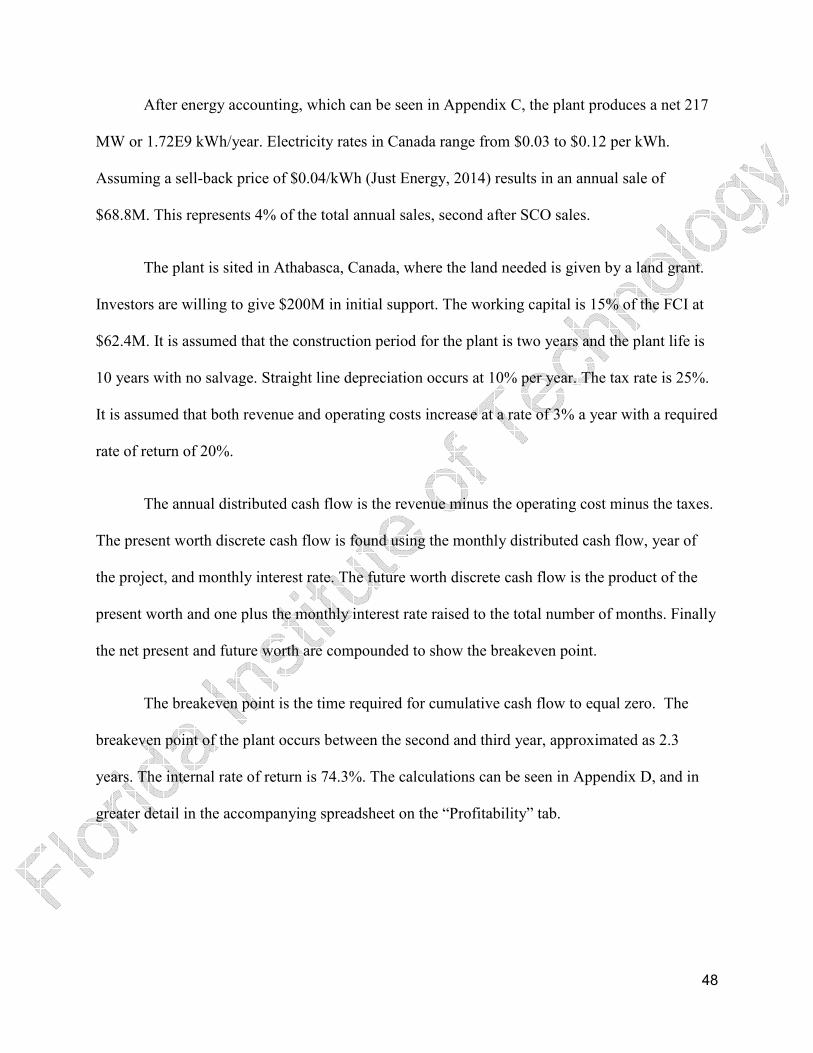
Figure 11: Effect of Varying Methane Price on Cumulative Profit

Table 22: Cumulative Profit Change from Change in Methane Price

Base Case $6.9B

+10%/yr $6.3B

+20%/yr $5.4B

The profitability was most impacted by a change in synthetic crude oil price. Given that

SCO is 92% of the yearly sales, it is assumed that the profitability depends solely on the SCO

price. If the oil price were to decrease by 5% per year compared to the base case of an increase

of 3% per year it resulted in an approximate $2.7 Billion reduction in cumulative profits, with the

addition of profit starting to level off at 12 years.

51

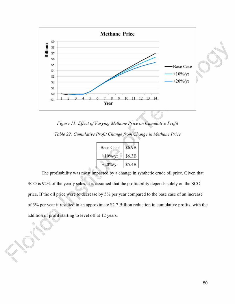
Figure 12: Effect of Varying Oil Price on Cumulative Profit

Given that oil prices are not very predictable, it was desired to model wild price

fluctuations. This was done in excel by changing the revenue input. Instead of the revenue

steadily increasing or decreasing, a random function generator was employed. The function

added the base sales from the electricity, sulfur and ammonia to the product of the yearly

production rate of oil and a random price generator. The range of the price generator was set

between $20 and $140 because those were the maximum and minimum prices seen during the

last decade. The Figure 13 shows a comparison of five random runs to the base case scenario.

52

Figure 13: Effect of Random Fluctuations in Oil Price on Cumulative Profit

Overall, the breakeven point does not change dramatically no matter what parameter is

examined. The breakeven point always occurs between the second and third year. It is only the

12 year cumulative profit that is sensitive to change.

Although this was not included in the analysis, the way the plant functions can also have

a strong effect on profitability. One of the faults in this simulation is that a well does not behave

nearly as simply as it is presented here. Production rate is a factor that changes with time as the

well becomes more developed or as it becomes depleted. As such, to accurately assess a plant’s

cumulative profitability would require the inclusion of these changing factors. In reality, these

factors are calculated and anticipated during operation such that changes to the flow rate to the

upgrading facility are mitigated against.

When a new well is drilled, part of that preparation to connect it to an in situ upgrading

facility including priming. Priming can involve a number of processes performed by field

engineers, such as the introduction of chemical agents as lubricants or corrosives and the direct

53

injection of high temperature and high pressure steam, even higher than that of a well in

production. This is accomplished by drilling teams using machinery, on site boilers, or steam

pipeline drawn out from the upgrading plant, forcing the plant to be unproductive until the well

is tapped (Stone and Bailey 2014). Without an outlet, heat and water is forced into tight

interstitial spaces between rock, soil, and the bitumen itself. After what can sometimes be weeks

to months of preparing a well, it is ready to be connected to production. New wells are less

productive as the well continues to loosen up; which can take upwards of a year (Laricina Energy

Ltd. 2010).

To mitigate this staggered production, wells are drilled and prepared in phases around a

destination production plant. As one particular well (phase 1) begins to deplete or otherwise

become unproductive, another well is in the process of becoming productive (phase 2); allowing

for a relatively seamless transition with little interruption to the facility or cash flow. As

mentioned, mitigating for this requires careful planning and expert knowledge of the geology,

gained from subterranean scanning by sonar, x-ray, or column sampling (Laricina Energy Ltd.

2010). This process has been omitted from this simulation for the sake of providing a simpler

basis from which to both work and present.

It should also be noted that synthetic crude oil is classified by sulfur content. SCO with

low sulfur content is classified as “sweet,” while oil with high sulfur content is considered

“sour”. The produced SCO would classify as sweet, and sweet synthetic crude oil makes up the

majority of the market (Bitumen, 2014).

54

Safety & Environmental

Compared to traditional coking, hydroconversion uses substantially less water, using less than

17% of the water coking uses (Munteanu, 2012). Conversely, the hydroconversion process

produces more CO2 - 77.3 kg CO2/bbl oil in comparison with 60 kg CO2/bbl oil for traditional

coking (Lightbown, 2014). Additional water and energy savings can be found by the use of

SAGD as opposed to other extraction methods. The once-steam generators (heaters) used to

make the steam typically generate 75 % steam and 25% hot water (Lui, 2006). Since SAGD

requires dry steam only, the water can be recovered for use in the heat exchangers. The water

coming out of the hydrotreaters can also be recycled. When the well is drilled for SAGD, the

well pairs are usually spaced 5-8 meters apart, with the lower producer well being of slightly

smaller diameter (Rach, 2004).

However, since there is a significant amount of steam required for any of the steam

extraction techniques the necessary energy input is fairly high. Burning natural gas for steam

heat and electricity generates a lot of CO2, much more than traditional bitumen extraction

methods (Nuwer, 2013). However, it is possible to do CO2 sequestration. This would not affect

the well since sequestration would be done at much greater depths than bitumen extraction.

Bitumen extraction is typically done at depths around 200m, while CO2 sequestration is done at

depths around 2000m (Palmgren 2011). In addition, the water drawn from the aquifer would not

be affected by either of these processes, since it is typically at depths of about double the depth

of the bitumen extraction process (EPA, 2013) (Ko, 2011).

Although this process does not use any solvents in the steam, if they were to be used it

would allow for the possibility of chemical seepage into the water table or atmosphere. In

addition, since SAGD pulls material from the ground, it can create void spaces which can

55

destabilize ground layers. Once a drilling operation ceases for a given reservoir, the mine can be

reclaimed by reintroducing the sand and related materials into the mine (EIS, 2012).

As for safety concerns, hydrogen sulfide gas can be dangerous to breathe if allowed to

reach certain concentrations. It is also highly corrosive. Symptoms include nausea, headaches,

etc., up to death depending on the concentration and length of exposure (OSHA, 2014). It can

also be explosive depending on concentration (2014). Ammonia is also highly corrosive and can

cause lung damage if inhaled in sufficient concentrations. Air concentration monitors will be

installed along with alarms at appropriate places within the plant.

As the SAGD gas will be highly pressurized and at high temperatures, precautions must

be taken and PPE must be worn. This is true for many if not all of the other processes, including

near the reactors. The bitumen itself is a skin irritant and studies differ on whether it is

carcinogenic (Wess, 2005). Since the reactors deal in high pressures and temperatures, properly

sized relief and rupture valves will need to be fitted.

56

Process Control

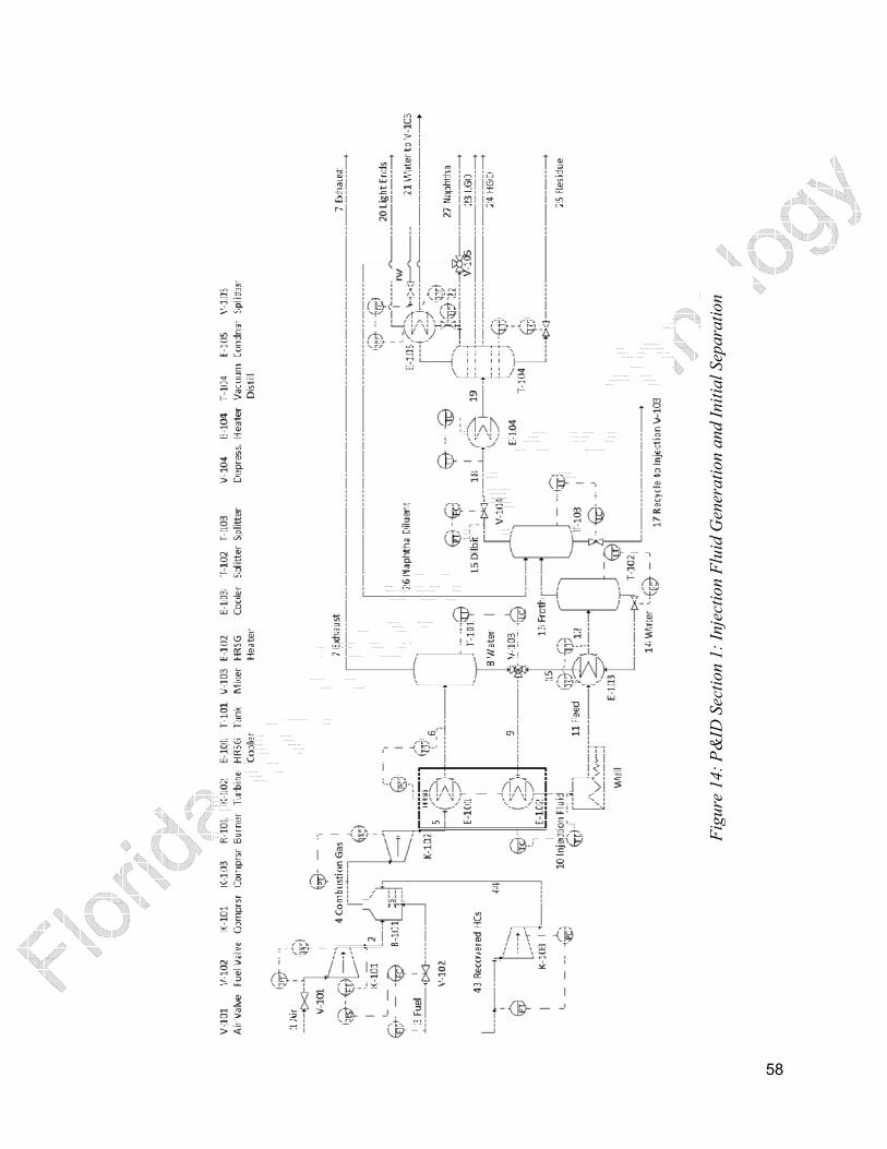
The P&ID can be found in Figures 14, 15, and 16 following this section. There is an air-

to-open valve prior to the compressor purely for safety shutdown purposes. The pressure of the

first compressor is controlled to ensure the appropriate pressure into the burner. The fuel is also

controlled by flow, but ratio control is imposed with an additional flow transmitter after the

compressor, to ensure the appropriate ratio of air to fuel into the burner. These valves are also

air-to-open. The other compressor (K-103) is also controlled to ensure proper pressure of

recovered hydrocarbons into the burner. The pressure exiting the compressor leading into the

HRSG is also controlled.

The pressure of the gases exiting the HRSG is controlled so as to not overtax the vessel

separating the exhaust gas from the exhaust water. The temperature of the steam exiting the

HRSG into the well is also controlled, as the heat diffusing into the surrounding sand/rock is the

primary mechanism which reduces the viscosity of the bitumen so that it can be pumped to the

surface. The pressure of the steam is also important and correlations can be made at a later date

between the control of the pressure of the exhaust gases exiting the HRSG and the temperature of

the steam.

The temperatures of various salt heat exchangers are controlled via electronic means. The

pressure exiting the pumps is also controlled electronically. For electronic controls, lines are

shown to enter directly into process equipment. Level controls are present on all separation

vessels, distillation columns, condensers, and reactors. Heat exchangers (or condensers) which

require cooling or refrigerated water or low pressure steam are temperature controlled based on

the exit temperature of the condenser. Compositions exiting each of the four reactors are

controlled based on the manipulation of flow rate of the hydrogen gas entering into the reactors.

57

However, it is important to bear in mind that hydrogen is usually supplied in excess. Note that

prior to most of the reactors, a molten salt heat exchanger’s outlet temperature is controlled

thereby ensuring the reactor temperature is appropriate.

Several valves are used to step-down pressure, and pressure controls are inserted to

facilitate this. The composition of the recovered hydrocarbons is controlled at the scrubber T-

106. The level control of the first vacuum distillation column is controlled by manipulating the

flow of the residue stream, since this is the largest stream exiting the column. Similarly, the level

control of the second vacuum distillation column is controlled by manipulating the flow of the

exiting light gas oil (Stream 38), as this is the stream with the largest fluid flow. The level

control of the mixing tank for the final SCO mixture is controlled by manipulating the exit flow

of the mixing tank. Finally, the pressure of the final dirty gas mixture stream is controlled for

downstream equipment.

The main control strategy is feedback control; however for further iterations it would be

advisable to include cascade control to reject disturbances in reactor temperature. In addition,

ratio control is applied to the fuel and air feed streams, however, there is a third stream

consisting of hydrocarbons recycled from further down the system. This is controlled only for

composition and pressure, however ideally a more advanced control which may utilize some

combination of ratio and/or cascade control should be implemented in future iterations. All

cooling water streams with valves are air-to-close to ensure that upon emergency conditions heat

flow is properly regulated. Similarly, streams with low pressure stream are controlled to be fail-

closed. Level controls on non-reactor equipment are air-to-open to reduce effect on downstream

equipment. Reactor controls are fail-open (air-to-close) so as to prevent reactions continuing to

occur in emergency situations. Compositional controls on hydrogen streams are also fail-closed.

58

Fig

ure

14:

P&

ID S

ecti

on 1

: In

ject

ion F

luid

Gen

erati

on a

nd I

nit

ial

Sep

ara

tion

59

Fig

ure

15:

P&

ID S

ecti

on 2

: H

ydro

cra

ckin

g a

nd S

econd S

epara

tion

60

Fig

ure

16:

P&

ID S

ecti

on 3

: C

om

ponen

t H

ydro

trea

tmen

t and F

inal

Pro

duct

Ble

nd

61

References

1. Alberta, Government of. (2014). Heavy Oil 101 - Upgrading and Refining. AERI.

AlbertaCanada.com. Retrieved from

http://www.albertacanada.com/mexico/documents/P7_Processing_Upgrading_and_Refini

ng_HOLA2013_KCY.pdf

2. Alibaba. (2014). Bitumen Pricing. Retrieved from

http://www.alibaba.com/Bitumen_pid100105

3. Alibaba. (2015). Ferric Sulfate Pricing. Retrieved from http://www.alibaba.com/product-

detail/ferric-sulphate_933493316.html

4. Alibaba. (2015). Industrial Ammonia Pricing. Retrieved from

http://www.alibaba.com/product-detail/industrial-liquid-ammonia-

price_1952696157.html

5. Alibaba. (2015). Yellow Sulphur Pricing. Retrieved from

http://www.alibaba.com/product-detail/sulphur_707085756.html

6. Aspentech. (2010). “Modeling Heavy Oil FAQ.”

7. Baker Hughes. (2013). SAGD Solutions. Retrieved from

https://www.youtube.com/watch?v=som4c1MIzAo

8. Barthe, P., et. al. (2015). Best Available Techniques (BAT) Reference Document for the

Refining of Mineral Oil and Gas. JCR Science and Policy Reports. Retrieved from

http://eippcb.jrc.ec.europa.eu/reference/BREF/REF_BREF_2015.pdf

9. Bhattacharjee, Subir. (2010). Oil Sands: A Bridge between Conventional Oil and a

Sustainable Energy Future. University of Alberta, Canada.

62

10. Bitumen Engineering. (2014). Synthetic Crude Oil Manufacturing by Upgrading Tar

Sand Bitumen. Retrieved from http://www.bitumenengineering.com/library/materials/41-

library/modifiedbituminousmaterials/115-synthetic-crude-oil-manufacturing

11. Bioage Group, LLC. (2013). AER Reports Recovery of 337,000 Gallons of Bitumen

from Surface Seeps at CNRL Primrose site; Earlier Event in 2009. Green Car Congress.

Retrieved from http://www.greencarcongress.com/2013/08/20130818-primrose.html

12. Bowman. (2015). Exhaust Gas Heat Exchangers. Retrieved from

http://www.ejbowman.co.uk/products/ExhaustGasHeatExchangers.htm

13. British Columbia Ministry of Finance. (2013). Tax Information Sheet. Retrieved from

http://www.sbr.gov.bc.ca/documents_library/shared_documents/Conversion_factors.pdf

14. Butler, R.M., McNab, G.S., and Lo, H.Y. (1981). Theoretical Studies on the Gravity

Drainage of Heavy Oil During In-Situ Steam Heating. The Canadian Journal of

Chemical Engineering 59 (4): 455-460. http://dx.doi.org/10.1002/cjce.5450590407

15. Calgary, University of. (2014). Unlocking the oil sands: The late Dr. Roger Butler,

Schulich School of Engineering. Calgary, Alberta. Retrieved from

http://www.ucalgary.ca/community/research/dr_roger_butlers

16. CAPP. (2014). CAPP Crude Oil Forecast, Markets & Transportation. Canadian

Association of Petroleum Producers.

17. EIS Information Center. (2012). Tar Sands Basics. 2012 Oil Shale & Tar Sands

Programmatic EIS. Information Center. Retrieved from

http://ostseis.anl.gov/guide/tarsands

63

18. El Gemayel, Gemayel. (2012). Integration and Simulation of a Bitumen Upgrading

Facility and an IGCC Process with Carbon Capture. Department of Chemical and

Biological Engineering. University of Ottowa.

19. Elliot, K., and Kovscek A. (2001). "A Numerical Analysis of the Single-Well Steam

Assisted Gravity Drainage Process (SW-SAGD)" Department of Petroleum Engineering,

Stanford University—U.S.A.

20. EPA. (2013). Carbon Dioxide Capture and Sequestration. Retrieved from

http://www.epa.gov/climatechange/ccs/

21. Eurobitume. (2014). Bitumen Production. Brussels, Belgium. Retrieved from

http://www.eurobitume.eu/bitumen/production-process

22. Glacier Media Inc. (2002). Cyclic Steam Outperforms SAGD at Cold Lake. New

Technology Magazine. Retrieved from

http://www.newtechmagazine.com/index.php/daily-news/archived-news/2974-cyclic-

steam-outperforms-sagd-at-cold-lake

23. Griffiths, Mary, Amy Taylor, and Dan Woynillowicz. (2006). Troubled Waters,

Troubling Trends - Technology and Policy Options to Reduce Water Use in Oil and Oil

Sands Development in Alberta. Pembina Institute. Retrieved from

https://www.pembina.org/reports/TroubledW_Full.pdf

24. Hart, A; Leeke, G; Greaves, M; Wood, J. (2014) Downhole heavy crude oil upgrading

using CAPRI: effect of steam upon upgrading and coke formation. American Chemical

Society. 28, 1811-1819.

64

25. Herzog, H. (2015) The Economics of CO2 Separation and Capture. MIT Energy

Laboratory. Retrieved from

http://sequestration.mit.edu/pdf/economics_in_technology.pdf

26. Indeck Keystone Energy, LLC. (2013). Indeck Keystone Energy - Waste Heat Recovery

Boilers. Retrieved from http://www.indeck-

keystone.com/waste_heat_recovery_boilers.htm

27. Jechura, John. (2014). Hydroprocessing: Hydrotreating and Hydrocracking. Colorado

School of Mines. Lecture.

28. Just Energy. (2014). Electricity and Natural Gas Rates for Athabasca, in Athabasca

Canada. American Dollars. Quote from Peter, 2/09/2014.

29. Kable Intelligence Limited. (2015). N2EG 32-16 Close-Coupled End-Suction Centrifugal

Pump. Varisco Solid Pumping Solutions. Hydrocarbons Technology. Retrieved from

http://www.hydrocarbons-technology.com/contractors/pumps/varisco/varisco4.html

30. Kawasaki Heavy Industries, Ltd. (2014). Plant and Infrastructure Company. Retrieved

from http://www.khi.co.jp/english/kplant/business/04_1.gif

31. Ko, Julia, and William Donahue. (2011). Drilling Down; Groundwater Risks Imposed by

In Situ Oil Sands Development. Water Matters Society of Alberta. Retrieved from

http://www.dirtyoilsands.org/wp-content/uploads/2014/06/drilling-down-july2011.pdf

32. Koscielnuk, D., et. al. Low Cost and Reliable Sulfur Recovery, J.C.S. Solutions and

MECS, Editors.

http://www.mecsglobal.com/Low%20Cost%20Reliable%20Sulfur%20Recovery.pdf

65

33. Ko, Julia, and William Donahue. (2011). Drilling Down; Groundwater Risks Imposed by

In Situ Oil Sands Development. Water Matters Society of Alberta. Retrieved from

http://www.dirtyoilsands.org/wp-content/uploads/2014/06/drilling-down-july2011.pdf

34. Laricina Energy Ltd. (2010). Breaking Through: West Athabasca Grand Rapids

Formation, Northeast Alberta, Canada. Presentation. Retrieved from

http://www.laricinaenergy.com/uploads/news/eage_06_10.pdf

35. Leffler, William. (2008). Petroleum Refining in Nontechnical Language. PennWell

Corporation. Google Book.

36. Lightbown, Vicki. (2014). New SAGD Technologies Show Promise in Reducing

Environmental Impact of Oil Sand Production. Oil and Gas Mining. Volume 1, Issue 2.

Retrieved from

http://albertainnovates.ca/media/20420/sagd_technologies_ogm_lightbown.pdf

37. Livingston, David. (2011). The Viability of Keystone XL: Of Politics, Profits, and

Pipelines. Athabasca Oil Sands Project. Retrieved from

http://leadenergy.org/2011/02/an-analysis-of-keystone-xl-of-politics-profits-and-

pipelines/

38. Lui, E.L. (Eddie). (2006). Imperial Oil – A Leader in Thermal In-situ Production.

Edmonton CFA Society Conference Investing in Alberta’s Oil Sands. Esso Imperial Oil.

Retrieved from http://www.imperialoil.ca/Canada-

English/files/News/N_S_Speech060608.pdf

39. Machine Mart. (2015). Clark Industrial Air Compressor - SE16C150. Retrieved from

https://www.machinemart.co.uk/shop/product/details/se16c150-air-

compressor/path/professionalindustrial-air-compressors-elect

66

40. Muarsulex. (2010). Sulfur & Petroleum Coke Markets. Calgary. SulfurUnit.com.

Coking.com. Retrieved from

http://www.sulfurunit.com/SeminarCanada/Presentations2010/Marsulex_DonBoonstra_S

ulphur&PetroleumCokeMarkets_Coking-SulfurUnitCom_Sep2010.pdf

41. Munteanu, Catalin Mugurel, and Jinwen Chen. (2012). Optimizing Bitumen Upgrading

Scheme – Modeling and Simulation Approach. Canmet Energy. Canada. 2012 AIChE

Spring Meeting, Houston, TX.

42. Noaman, Amed. (2013). Enhanced Oil Recovery Using Steam. COMSATS Institute of

Information Technology, Lahore. SlideShare. Retrieved from

http://www.slideshare.net/NomanAhmed1/enhanced-oil-recovery-steam-recovery

43. NSERC. (2015). Water Quality - NSERC Industrial Research Chair Website. Water

Quality Management for Oil Sands Extraction. Retrieved from

http://www.oilsands.ualberta.ca/wqm/?page_id=19

44. Nuwer, Rachel. (2013). Oil Sands Mining Uses Up Almost as Much Energy as it

Produces. Inside Climate News. Retrieved from

http://insideclimatenews.org/news/20130219/oil-sands-mining-tar-sands-alberta-canada-

energy-return-on-investment-eroi-natural-gas-in-situ-dilbit-bitumen

45. Oil-Price.net. (2014). Crude Oil and Commodity Prices. Retrieved from http://www.oil-

price.net/index.php?lang=en

46. Oil Review Africa. (2010). Optimizing Heavy Oil Steam Drainage Scenarios. Issue One,

pg 93. Alain Charles Publishing Ltd.

47. Ondrey, Gerald. (2012). Athabasca Oil selects GE’s water-treatment technologies for

SAGD project. Chemical Engineering Online. Retrieved from

67

http://www.chemengonline.com/athabasca-oil-selects-ges-water-treatment-technologies-

for-sagd-project

48. OSHA. (2014). Hydrogen Sulfide. Safety and Health Topics. United States Department

of Labor. https://www.osha.gov/SLTC/hydrogensulfide/hazards.html

49. Palmgren, C., I. Walker; M. Carlson, M. Uwiera, and M. Torlak. (2011). Reservoir

Design of a Shallow LP-SAGD Project for In Situ Extraction of Athabasca Bitumen.

World Heavy Oil Congress. Edmonton, Alberta. Retrieved from

http://www.aboilsands.ca/_pdfs/Technical-Presentations/Papers/Shallow-LP-SAGD-

Extraction-Bitumen.pdf

50. Payscale. (2015). Process Engineer Salary. Median Salary. Canada. Retrieved from

http://www.payscale.com/research/CA/Job=Process_Engineer/Salary

51. Peck, E. (1941). Regeneration of Spent Catalysts. U.S. Patent. March 1, 1941.

52. Pembina Institute. (2010). Water Impacts. Oil Sands 101. Retrieved from

http://www.pembina.org/oil-sands/os101/water

53. Peng, D. Y., and Robinson, D. B. (1976). "A New Two-Constant Equation of State".

Industrial and Engineering Chemistry: Fundamentals 15: 59–64.

54. Platts, Sydney. (2015). Oil Sector Faces ‘Toughest Year in a Generation’ but Prices Will

Recover: Bernstein. McGraw Hill Financial. Retrieved from

http://www.platts.com/latest-news/oil/sydney/oil-sector-faces-toughest-year-in-a-

generation-27996525

55. Rach, Nina M. (2004). SAGD drilling parameters evolve for oil sands. Oil & Gas

Journal; 102, 21; Proquest. Pg 53.

68

56. Shell. (2011). Redeveloping Schoonebeek Oilfield with New Technologies. Retrieved

from https://www.youtube.com/watch?v=6IFHzCmbwqU

57. Song, Lisa. (2012). A Dilbit Primer: How It's Different from Conventional Oil.

InsideClimate News. Retrieved from http://insideclimatenews.org/news/20120626/dilbit-

primer-diluted-bitumen-conventional-oil-tar-sands-Alberta-Kalamazoo-Keystone-XL-

Enbridge

58. Speight, James. (2007). Hydroprocessing of Heavy Oils and Residua. Pg 134.

59. Stone, T. and Bailey, W. (2014). Optimization of Subcool in SAGD Bitumen Processes.

World Heavy Oil Congress 2014. Conference proceedings. Retrieved from

http://www.slb.com/~/media/Files/technical_papers/whoc/WHOC14-271.pdf

60. Sundram, et al. (2013). Systems and Methods for Creating a Model of Composition for a

Composite Formed by Combining a Plurality of Hydrocarbon Streams. Patent. Retrieved

from http://www.google.com/patents/WO2013181078A1?cl=en

61. Surmont Energy. (2011). (SAGD) Steam Assisted Gravity Drainage - Oil Sands

Extraction. Retrieved from https://www.youtube.com/watch?v=uucXaKK-EnY

62. Tomadakis, Manolis. (2014) Separations Notes Part 1. CHE 4131. Florida Institute of

Technology.

63. Turton, Richard, Richard Bailie, Wallace Whiting, and Joseph Shaeiwitz. (2008).

Analysis, Synthesis, and Design of Chemical Processes. 3rd Edition. Appendix A. Cost

Equations and Curves for the CAPCOST Program.

64. Turton, Richard, Richard Bailie, Wallace Whiting, and Joseph Shaeiwitz. (2008).

Analysis, Synthesis, and Design of Chemical Processes. 3rd Edition. Chapter 9

Heuristics Tables.

69

65. Vega. (2003). Level Measuring System for Hydrofluoric Acid - Contactless and

Extremely Resistant. Distillation Column. Retrieved from

http://www.vega.com/en/Application-newsletter_40026.htm

66. Wess, Joann, A., and Dr. Larry Olsen. (2005). Asphalt (Bitumen). World Health

Organization. Retrieved from

http://www.who.int/ipcs/publications/cicad/cicad59_rev_1.pdf

67. White, John, et al. (2012). RF heating to reduce the use of supplemental water added in

the recovery of unconventional oil. Patents. Retrieved from

http://www.google.com.ar/patents/US8128786

68. Wintershall. (2015). Oil Can Do More - Crude Oil is the Most Important Material of the

Industrialized Nations. Wintershall Holding GmbH. Retrieved from

http://www.wintershall.com/en/company/oil-and-gas/oil-can-do-more.html

69. Vacuum Distillation of Atmospheric Residues. (2009). Encyclopedia of Hydrocarbons.

Volume II Refining and Petrochemicals. Distillation Processes. Pgs 108-112.

70

Appendix A: All Equipment Design Methods, Calculations and Assumptions

Injection

Figure 17: HYSYS Injection Simulation

Air was assumed to be compressed from ambient conditions and concentrations before

being added to the burner. Methane fuel was assumed to be delivered from a compressed source

at 2500 kPa, whether that was from storage or a pipeline was not pertinent to the simulation. The

source fuel is mixed with recycled hydrocarbons compressed to equal pressure before being

added to the burner. It was decided the packaged Gibb’s equations were sufficient for

combustion simulation. Expander turbine K-102 generates the electricity used by the plant and

the excess sold off, Q-101.

71

HRSG

Figure 18: HYSYS HRSG Simulation

Shown in energy stream Q-103 is the direct enthalpy connection between the two units to

simulate the behavior of an HRSG unit. R-102 is the HYSYS feeder block, which provides

characterized petroleum assay components to the influent stream. This means that mass is

effectively added to the system at the feeder block, which does the job of representing mass

added to the system by the bitumen well.

72

Darcy Theory

The well is also modeled using Darcy theory:

Darcy Travel Time Ratio Derivation

9 = −�CD

9� = −�� EFEG 9H = −�H EFEI

9� = ��∆KL 9H = −�H E�EI

�� = MNMOPQP �H = MRMOPQP

9� = MNMOPQP ∆KL 9H = − MRMOPQPE�EI

.� = HSN .H = ?SR

HTN = MNMOPQP ∆KL ?TR = − MRMOPQP

E�EI

.� = QPMNMOPH∆UV .H = − QPMRMOP

?W(�XYZ[�\O]^)

.�.H = _8� `H`�(�a+b − �BcdE)∆KL

Figure 19: Darcy Theory

U Darcy velocity

K Overall permeability

Ψ Resistive forces

Xv Denotes property is in vertical dimension

Xh Denotes property is in horizontal dimension

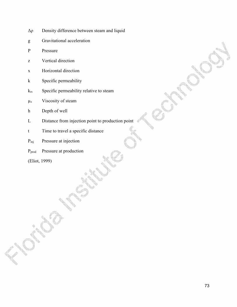
73

Δρ Density difference between steam and liquid

g Gravitational acceleration

P Pressure

z Vertical direction

x Horizontal direction

k Specific permeability

krs Specific permeability relative to steam

µs Viscosity of steam

h Depth of well

L Distance from injection point to production point

t Time to travel a specific distance

Pinj Pressure at injection

Pprod Pressure at production

(Eliot, 1999)

74

Settlers

Figure 20: HYSYS Settler Simulation

Figure 21: 1st Settler Components in HYSYS

75

Shown here are the component splitter blocks used for the settling tanks. The window

shows how a user can set ratios of components to be send to different streams. Here T-102

separated 91% by mole of water to a pure water stream, leaving 9% entrained in bitumen froth

awaiting diluent assisted separation.

Distillation

Figure 22: HYSYS Vacuum Distillation Column Simulation

Shown is a vacuum distillation column, showing the cuts of naphtha, HGO, LGO, and

residue. Notice the recycle of part of the naphtha stream to the beginning of the system, used to

enhance the separation of the water from the bitumen froth in the second settler.

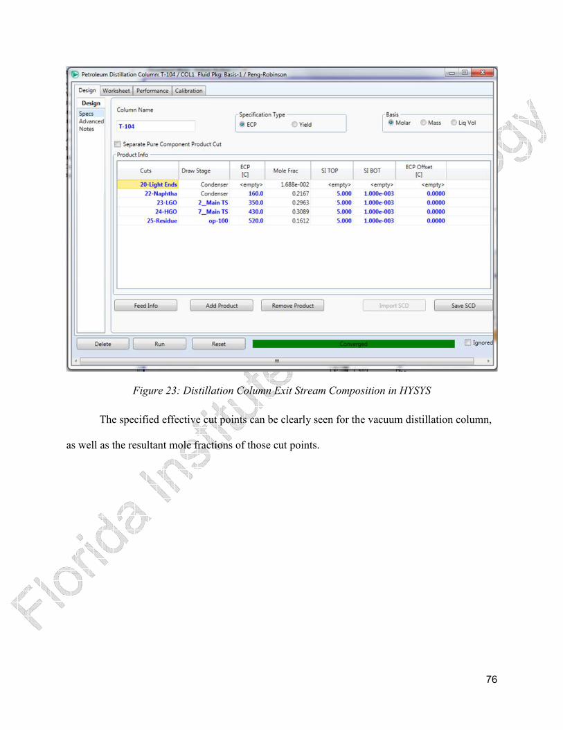
76

Figure 23: Distillation Column Exit Stream Composition in HYSYS

The specified effective cut points can be clearly seen for the vacuum distillation column,

as well as the resultant mole fractions of those cut points.

77

Hydrocracker

Figure 24: HYSYS Hydrocracker

Shown here is the HYSYS block arrangement which was used to apply Excel black box

values to the process.

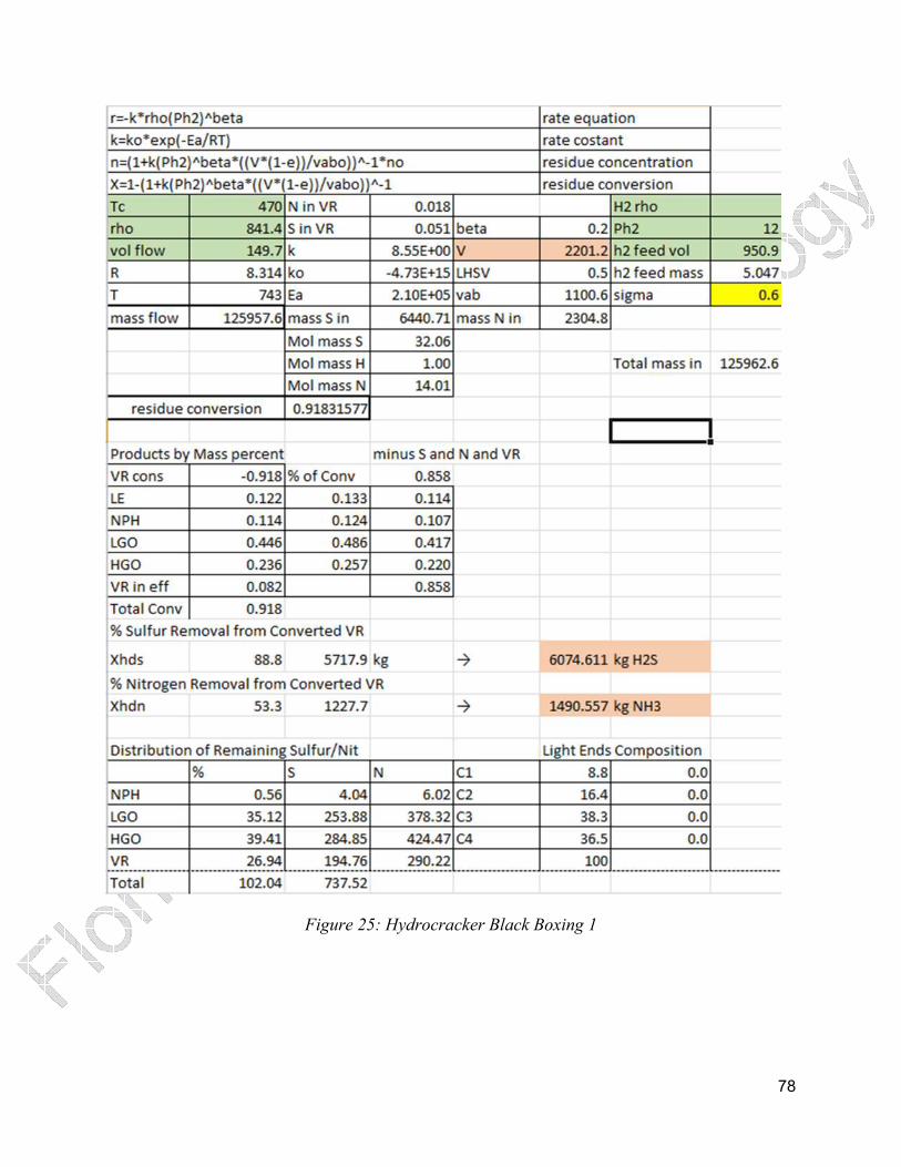
78

Figure 25: Hydrocracker Black Boxing 1

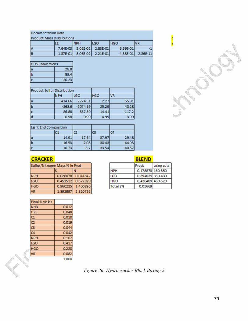
79

Figure 26: Hydrocracker Black Boxing 2

80

Figures 25 and 26, as seen above, show the black boxing done in Excel.

Figure 27: HYSYS Hydrotreaters

Similarly to the hydrocracker, a petroleum shift reactor was used to input the appropriate

exit stream conditions into the simulation for the three hydrotreaters.

81

Figure 28: Hydrotreaters Black Boxing 1

Figure 29: Hydrotreaters Black Boxing 2

82

Figure 30: Hydrotreaters Black Boxing 3

As seen in Figures 28, 29 and 30, the black boxing was done in Excel for each of the

three hydrotreaters.

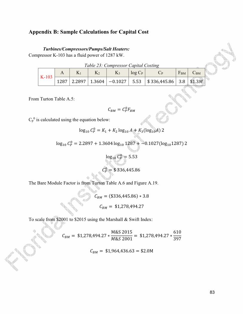
83

Appendix B: Sample Calculations for Capital Cost

Turbines/Compressors/Pumps/Salt Heaters:

Compressor K-103 has a fluid power of 1287 kW.

Table 23: Compressor Capital Costing

K-103 A K1 K2 K3 log CP CP FBM CBM

1287 2.2897 1.3604 −0.1027 5.53 $ 336,445.86 3.8 $1.36

From Turton Table A.5:

��� = ������

Cp0 is calculated using the equation below:

log� ��� = � + �� log� � + ��(log��) 2

log� ��� = 2.2897 + 1.3604 log� 1287 + −0.1027(log�1287) 2

log� ��� = 5.53

��� = $ 336,445.86 The Bare Module Factor is from Turton Table A.6 and Figure A.19.

��� = ($336,445.86) ∗ 3.8

��� = $1,278,494.27

To scale from $2001 to $2015 using the Marshall & Swift Index:

��� = $1,278,494.27 ∗ M&S 20156&j 2001 = $1,278,494.27 ∗ 610397

��� = $1,964,436.63 = $2.0M

84

Reactors:

The burner R-101 is part of a gas turbine. Its cost is assumed to be included in the cost of

the compressor and turbine K-101 and K-102.

The hydroconverter and hydrotreaters were cost as towers, because of the high pressure

and high capacities required. Each reactor volume was found using the volumetric flow rate in

and the LHSV given by El Gemayel and Speight.

LGO hydrotreater R-104 has a LHSV of 2.5/h and a volumetric flow rate inlet of 193.2

m3/h. The capacity of the reactor for costing purposed is the volume.

k = la+8mjk = 193.2 n�_2.5/_ = 77.28n�

Table 24: Reactor Costing

R-104

A K1 K2 K3 log CP CP

77.28 3.4974 0.4485 0.1074 4.73 $ 53,340.53 FM FP B1 B2 P (barg) CBM ($2001)

3.1 17.69 2.25 1.82 54.3 $ 5.46 CBM ($2015) $8.46

��� = ������ = ���( + �����) Cp

0 is calculated using the equation below:

log� ��� = � + �� log� � + ��(log��) 2

log� ��� = 3.4974 + 0.4485 log� 77.28 + 0.1074(log�77.28) 2

log� ��� = 7.73

��� = $ 53,340.53 As a tower, FP is calculated using the pressure and diameter, D. The diameter of the

reactor is calculated assuming a reactor length to diameter ratio of 3.

k = pq�8 = p ��4 8 = p ��

4 3� = 3p4 ��

85

� = r4k3ps = r4 ∗ (77.28n�)3ps = 3.2n

��,������ =(� + 1)�2[850 − 0.6(� + 1)] + 0.00315

0.0063 =(54.3tuqL + 1) ∗ (3.2n)2[850 − 0.6(54.3tuqL + 1)] + 0.00315

0.0063

��,������ = 17.69

Then using the material factor and constants B1 and B2:

��� = ���( + �����) = $ 53,340.53 ∗ (2.25 + 1.82 ∗ 3.1 ∗ 17.69)

��� = $ 5,444,992.65 To scale from $2001 to $2015 using the Marshall & Swift Index:

��� = $ 5,444,992.65 ∗ M&S 20156&j 2001 = $ 5,444,992.65 ∗ 610397

��� = $8,366,361.50 = $8.4M Towers:

Some towers were cost as process vessels due to their size. The volumes of the towers

were found by a provided contact time, and if no contact time was found, it was assumed to be a

hold-up of 5 minutes (Turton, 2008). The volume was then used to find the diameter and length

using the same process as above.

In the case of T-102, it needed to be scaled up, because its capacity fell outside of the

range listed for process vessels. The following equation was used, where � is the cost, u refers to

the smaller unit, t is the new unit, � is the capacity, and v is the cost exponent. For T-102, the

662m3 vessel was cost as a 628m3 vessel of $1,239,508.19. A cost exponent of 0.6 from Turton

was used.

�'�( = )�'�(*+

86

$1,239,508.19�( = w628n�662n�x+

�( = $1,279,470.34 Two towers were packed distillation columns. These were cost as towers with packing.

For example, T-104. The capacity of a tower for costing purposes is volume. The volume of the

tower was found using the diameter from Aspen modeling and the calculated height. The height

is based on tray spacing, j, multiplied by the number of stages, v, plus the ceiling and buffer

zone heights (Tomadakis, 2014).

m = vj + � + = 24 ∗ 1.2n + 1.2n + 4.3n = 34.3n

k = p ��4 m = p (11.65n)�

4 (34.3n) = 3656.2n�

This volume is outside the range for towers (maximum 520 m3) so the final bare module

cost will need to be scaled up. The same procedure to cost a vessel is used to cost a tower.

Table 25: Tower Costing

T-104

A K1 K2 K3 log CP CP

520 3.4974 0.4485 0.1074 5.51 $ 321,945.46 FM FP B1 B2 P (barg) CBM ($2001)

3.1 0.78 2.25 1.82 0.002 $ 2.16 CBM ($2001) Scaled CBM ($2015) Scaled

$ 6.86 $10.46

The packing for T-104 is metal grid-packed Raschig P90X. The costing follows the same

basic procedure.

Table 26: Packing Costing

T-104 Packing

A K1 K2 K3 log CP CP

160.7 2.4493 0.9744 0.0055 4.63 $ 42,228.69 FM FP log FP C1 C2 C2

7.1 1 0 0 0 0 CBM ($2001) CBM ($2015)

$ 0.306 $0.466

87

Heat Exchangers:

The areas for the heat exchangers were found via modeling in Aspen Plus V8.6. The process

streams composition, flow rate, temperature, pressure, and calculated duty were taken from

HYSYS. The heavier oil streams were approximated as molar fractions of 0.69 linoleic acid, 0.26

oleic acid and 0.05 stearic acid. This ratio is found in soy bean oil ignoring less common

constituents. This is likely ineffective for naphtha and HGO, but very close to LGO and is a

source of error in costing the heat exchangers. Light ends were substituted with iso-butane,

which accurately follows the average molecular weight of the light ends.

Specific exchangers were set as salt heaters because of the required temperatures. The high

temperatures needed would have required copious amounts of very high pressure and

temperature steam. Given that our injection process generates power, it is more cost effective to

model these exchangers as electric salt heaters.

Ferric Sulfate Cost �y�W(z>{)s = (1 − |�daE) ∗ kc�'}Tdc� ∗ K}'T ∗ �,-.}'T= (1 − 0.37) ∗ 496.76n� ∗ 3100`Ln� ∗ 0.2996 $`L = $290,627.81

88

Table 27: Capital Costing Spreadsheet 1

Did not use correct values, I

used values I assumed, will

need to go back and correct

Maximum

capacity, scaled

up to the far right

pressure out of range in turton

Material Selection Capacity K1 K2

K-101 compr. centrifugal wo drive, ss 3000 2.2897 1.3604

K-102 axial gas turbine 4000 2.7051 1.4398

K-103 compr. centrifugal wo drive, ss 1287 2.2897 1.3604

HRSG (E-101/E/102)

R-101gas turbine burner (assumed cost is accounted for in the compressor and turbine)

R-102 cracker, as tower ss 202.2 3.4974 0.4485

R-103 treater, as tower ss 18.786 3.4974 0.4485

R-104 treater, as tower ss 77.28 3.4974 0.4485

R-105 treater, as tower ss 198.5 3.4974 0.4485

T-101 vertical vessel, ss clad 355.3 3.4974 0.4485

T-102 horizontal vessel, ss clad 628 3.5565 0.3776

T-103 tank API fixed roof 5840 4.8509 -0.3973

T-104

column as tower, assuming 24

stages520 3.4974 0.4485

packing

packing, grid-pack, rashig,

metal, P90X160.7 2.4493 0.9744

T-105 column as tower 520 3.4974 0.4485

packing

packing, grid-pack, rashig,

metal, P90X46.9 2.4493 0.9744

T-106 absorber, verticle vessel 7.365 3.4974 0.4485

E-103 U-tube, Cs/Cs 1000 4.1884 -0.2503

E-104 electric heater, molten salt 10750 1.1979 1.4782

E-105 refrigerated water, u-tube 2659 4.1884 -0.2503

E-106 electric heater, molten salt 5047 1.1979 1.4782

E-107 U-tube, cs shell/ss tube 62.4 4.1884 -0.2503

E-108 refrigerated water, u-tube 749.5 4.1884 -0.2503

E-109 double pipe, SS tube/CS shell 1.3 3.3444 0.2745

E-110 U-tube, cs shell/ss tube 101 4.1884 -0.2503

E-111 electric heater, molten salt 8206 1.1979 1.4782

E-112 electric heater, molten salt 2846 1.1979 1.4782

E-113 U-tube, cs shell/ss tube 2581 4.1884 -0.2503

E-114 U-tube, cs shell/ss tube 4194 4.1884 -0.2503

E-115 U-tube, cs shell/ss tube 4413 4.1884 -0.2503

P-101

centrifugal, *pressure out of

range300 3.3892 0.0536

P-102 centrifugal 300 3.3892 0.0536

P-103 centrifugal 300 3.3892 0.0536

P-104

centrifugal, *pressure out of

range300 3.3892 0.0536

89

Table 28: Capital Costing Spreadsheet 2

This values are

very high?

K3 Log Cp CP CBM Fm or Fbm Fp (or Fq) Log Fp (Fq) B1 B2

-0.1027 5.78 600,197.98$ 2,280,752.32$ 3.8 1 0 - -

-0.1776 5.59 386,380.38$ 533,204.93$ 1.38 1 0 - -

-0.1027 5.53 336,445.86$ 1,278,494.27$ 3.8 1 0 - -

in 2010 $ 12,659,000.00$

0.1074 5.10 126,633.48$ 52,922,128.16$ 3.1 73.67 - 2.25 1.82

0.1074 4.24 17,497.97$ 683,700.03$ 3.1 6.53 - 2.25 1.82

0.1074 4.73 53,340.53$ 5,444,992.65$ 3.1 17.69 - 2.25 1.82

0.1074 5.09 124,447.37$ 37,763,986.00$ 3.1 53.39 - 2.25 1.82

0.1074 5.34 218,794.55$ 1,509,005.63$ 1.7 1.50 - 2.25 1.82

0.0905 5.32 209,650.49$ 1,239,508.19$ 1.7 1.71 - 1.49 1.52

0.1445 5.40 253,724.13$ 1,355,901.76$ 1.7 1.00 0 2.25 1.82

0.1074 5.51 321,945.46$ 2,142,763.95$ 3.1 0.78 - 2.25 1.82

0.0055 4.63 42,228.69$ 299,823.73$ 7.1 1.00 0

0.1074 5.51 321,945.46$ 2,377,473.91$ 3.1 0.91 - 2.25 1.82

0.0055 4.09 12,389.43$ 87,964.95$ 7.1 1.00 0

0.1074 3.97 9,270.23$ 45,707.59$ 1.9 0.78 - 2.25 1.82

0.1974 5.21 163,719.35$ 551,070.06$ 1 1.05 0.019 1.63 1.66

-0.0958 5.60 398,255.74$ 836,337.04$ 2.1 1.00 0.000 - -

0.1974 5.65 443,034.48$ 2,045,933.24$ 1.8 1.00 0.000 1.63 1.66

-0.0958 5.36 228,071.27$ 558,164.03$ 2.1 1.17 0.066 - -

0.1974 4.38 23,725.96$ 109,566.50$ 1.8 1.00 0.000 1.63 1.66

0.1974 5.10 125,956.28$ 581,666.12$ 1.8 1.00 0.000 1.63 1.66

-0.0472 3.38 2,371.73$ 10,743.92$ 1.8 1.00 0.000 1.74 1.55

0.1974 4.48 30,181.04$ 139,376.04$ 1.8 1.00 0.000 1.63 1.66

-0.0958 5.52 328,150.02$ 771,434.92$ 2.1 1.12 0.049 - -

-0.0958 5.16 144,840.31$ 346,121.87$ 2.1 1.14 0.056 - -

0.1974 5.63 428,769.78$ 2,145,371.49$ 1.8 1.13 0.053 1.63 1.66

0.1974 5.87 745,113.64$ 3,956,685.33$ 1.8 1.23 0.090 1.63 1.66

0.1974 5.90 791,410.04$ 4,687,436.52$ 1.8 1.44 0.157 1.63 1.66

0.1538 4.47 29,222.03$ 228,099.41$ 1.5 2.92 0.466 1.89 1.35

0.1538 4.47 29,222.03$ 147,908.10$ 1.5 1.57 0.195 1.89 1.35

0.1538 4.47 29,222.03$ 170,407.23$ 1.5 1.95 0.289 1.89 1.35

0.1538 4.47 29,222.03$ 209,928.51$ 1.5 2.61 0.417 1.89 1.35

TOTAL 194,584,018.07$

New Cost 352,273,627.87$

415,682,880.89$ Total Module Cost

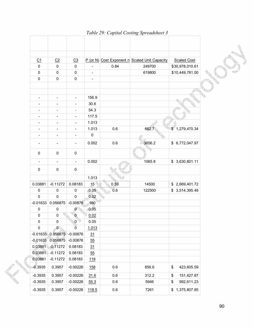
90

Table 29: Capital Costing Spreadsheet 3

C1 C2 C3 P (or N) Cost Exponent n Scaled Unit Capacity Scaled Cost

0 0 0 - 0.84 249700 30,978,010.61$

0 0 0 - 619800 10,449,781.00$

0 0 0 -

- - - 156.9

- - - 30.6

- - - 54.3

- - - 117.5

- - - 1.013

- - - 1.013 0.6 662.7 1,279,470.34$

- - - 0

- - - 0.002 0.6 3656.2 6,772,047.97$

0 0 0

- - - 0.002 1065.8 3,630,801.11$

0 0 0

1.013

0.03881 -0.11272 0.08183 15 0.59 14500 2,669,401.72$

0 0 0 0.05 0.6 122500 3,514,395.48$

0 0 0 0.02

-0.01633 0.056875 -0.00876 160

0 0 0 0.05

0 0 0 0.02

0 0 0 0.05

0 0 0 1.013

-0.01633 0.056875 -0.00876 31

-0.01633 0.056875 -0.00876 55

0.03881 -0.11272 0.08183 31

0.03881 -0.11272 0.08183 55

0.03881 -0.11272 0.08183 119

-0.3935 0.3957 -0.00226 158 0.6 856.6 423,605.59$

-0.3935 0.3957 -0.00226 31.6 0.6 312.2 151,427.87$

-0.3935 0.3957 -0.00226 55.3 0.6 5946 992,611.23$

-0.3935 0.3957 -0.00226 118.5 0.6 7261 1,375,807.85$

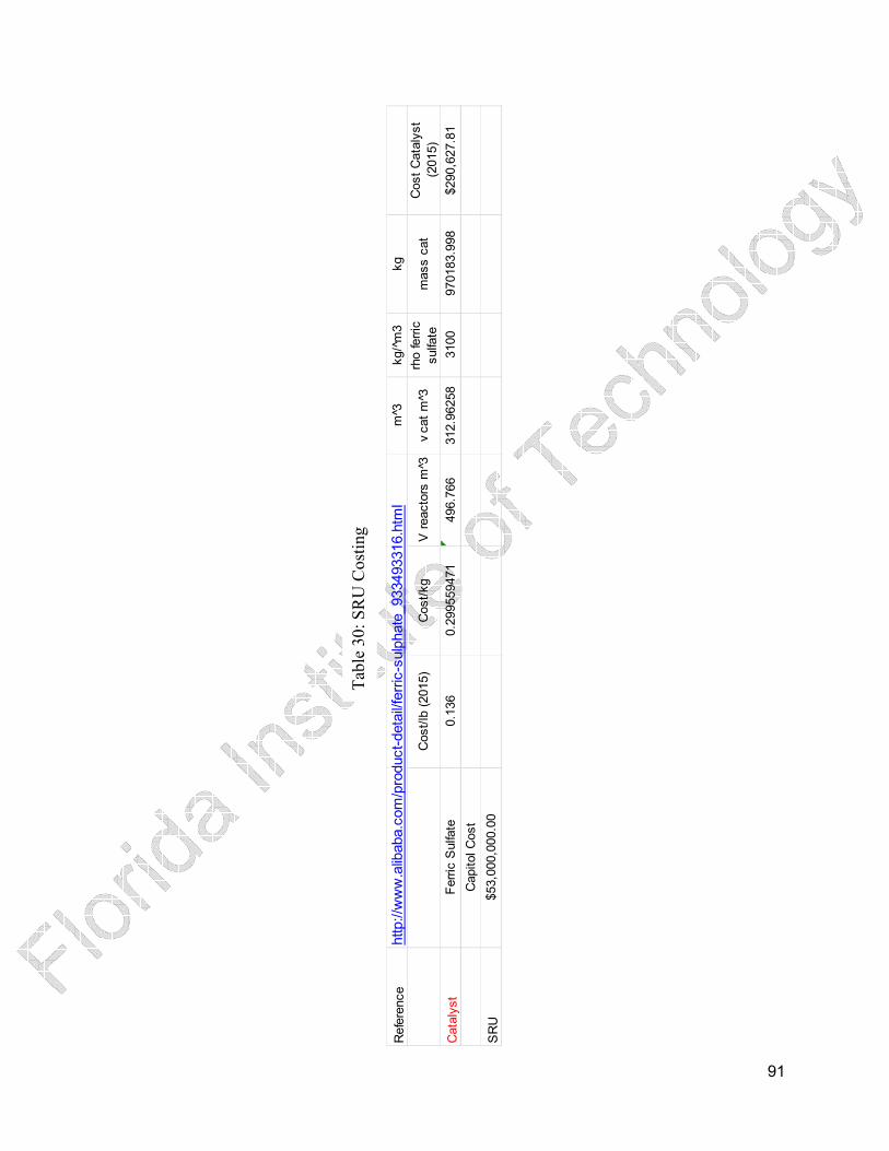
91

Refe

rence

http://w

ww

.alib

aba.c

om

/pro

duct-

deta

il/fe

rric

-sulp

hate

_933493316.h

tml

m^3

kg/^

m3

kg

Cost/

lb (

2015)

Cost/

kg

V r

eacto

rs m

^3v

cat

m^3

rho ferr

ic

sulfa

tem

ass c

at

Cost

Cata

lyst

(2015)

Cata

lyst

Ferr

ic S

ulfa

te0.1

36

0.2

99559471

496.7

66

312.9

6258

3100

970183.9

98

$290,6

27.8

1

Capitol C

ost

SR

U$53,0

00,0

00.0

0

Tab

le 3

0:

SR

U C

ost

ing

92

Appendix C: Sample Calculations for Manufacturing Cost

Refrigerated Water Cost

�c~ = 3288 `n,�_q ∗ 0.018 `L`n,� ∗ 24 _q�u� ∗ 330 �u��q ∗ 0.00018 $`L ∗ 578.4 2015 �0��1499.6 2006 �0��1 = $100.39

93

Table 31: Manufacturing Cost Spreadsheet

Bitumen McCuskey, Frandsen, Hogan

Direct Fixed Generalcost f(production) independent or loose loose

raw materials taxes & insurance sales/marketing

utilities depreciation R&D

labor plant overhead ->cost of running facilitiesAdmin

waste treatment

supplies

maintenance

lab charges

patents & royalties

For Direct (DMC), we need: 2015

From Capitol Cost Asmt FCI $415,682,880.89

Raw materials cost CRM 194,918,590.91$

Waste Treatment CWT 41,393,088.00$

Utilities CUT 100.39$

Operating Labor COL 2,547,526.95$

Direct Supervisory/Clerical Labor (0.18)*COL $458,554.85

Maintenance and Repairs (0.06)*FCI $24,940,972.85

Operating Supplies (0.009)*FCI $3,741,145.93

Lab Charges (0.15)*COL $382,129.04

Patents and Royalties (0.3)*COM 0

Total DMC = CRM + CWT + CUT +(1.33)*COL + (0.03)*COM + (0.069)*FCI $268,382,108.93

Fixed Manufacturing Cost (FMC)

Depreciation (0.1)*FCI $41,568,288.09

Local Taxes and Insurance (0.032)*FCI $133,018,521.88

Plant Overhead Costs (0.708)*COL+(0.036)*FCI $16,768,232.79

Total FMC = 0.708*COL + 0.068*FCI $30,070,084.98

General Manufacturing Expenses

Administration costs (0.177)*COL+(0.009)*FCI $4,192,058.20

Distribution and Selling costs (0.11)*COM $40,968,527.12

Research and Development (0.05)*COM $18,622,057.78

Total GMC=0.177*COL+0.009*FCI+0.16*COM $4,192,058.20

Total Costs = CRM + CWT +CUT +(2.215)*COL + (0.190)*COM + (0.146)*FCI $373,408,071.69

Sales

COM = 0.18FCI + 2.73COL + 1.23(CUT + CWT + CRM) = 372,441,155.68$ $1,667,328,055.20

Cost of Manufacturing (COM)

94

CR

M

Vo

lum

e m

3/h

rG

J/hr

Cost/

hr

Cost/

year

(2015)

$m

eth

ane/G

J

Meth

ane (

for

burn

er)

111100

4251.8

17834

$17,0

07.2

7$134,6

97,5

88.9

84

Hydro

gen

BB

L o

il/day

H2 n

eeded s

cf/bbl

H2 s

cf used/d

ay

H2 s

cf used/y

ear

Price $

/1000 s

cf

Cost/

year

(2015)

R-1

03 (

Hydro

gra

cker)

**

21570

1836

39602520

13068831600

$1.7

3$22,6

35,2

16.3

3

R-1

04 (

NP

H H

ydro

treate

r)14440

400

5776000

1906080000

$1.7

3$3,3

01,3

30.5

6

R-1

05 (

NP

H H

ydro

treate

r)29410

800

23528000

7764240000

$1.7

3$13,4

47,6

63.6

8

R-1

06 (

NP

H H

ydro

treate

r)30380

1200

36456000

12030480000

$1.7

3$20,8

36,7

91.3

6

Tota

l$60,2

21,0

01.9

3

CR

M (

2015)

$194,9

18,5

90.9

1

CO

L

P=

1 b

ecause t

he first

sett

ler

dis

poses o

f sand fro

m t

he w

ell

Sulfu

r R

ecove

ry U

nit

Nnp -

add e

ach e

quip

ment

25

Nnp

6

NO

L =

sqrt

(6.2

9+

37.1

P2̂+

0.2

3N

np)

7.0

09992867

NO

L =

sqrt

(6.2

9+

37.1

P2̂+

0.2

3N

np)

2.7

69476485

Multip

ly t

his

# b

y 4

.5 s

hift

s31.5

449679

Multip

ly t

his

# b

y 4

.5 s

hift

s12.4

6264418

Roundin

g u

p32

Roundin

g u

p13

Pay p

er

Year

C$

$69,8

91.0

0S

lide 1

5 h

as e

xam

ple

Pay p

er

Year

C$

$69,8

91.0

0

In U

SD

$56,6

11.7

1In

US

D$56,6

11.7

1

Bitum

en p

lant

CO

L$1,8

11,5

74.7

2C

OL

$735,9

52.2

3

CO

L A

CTU

AL (

2015)

$2,5

47,5

26.9

5

Table

32:

Raw

Mate

rials

and C

ost

of

Labor

95

CU

T

Equpim

ent

ID (

condensers

)R

efrig

. W

ate

r (k

mol/hr)

Refrig

. W

ate

r (k

g/h

r)kg/y

rP

rice (

$/k

g)

of re

frig

Cost

($/y

r)Tota

l cost/

yr

2006

Tota

l C

ost

(2015)

E-1

05

2530

45.5

4360676.8

0.0

00185

66.7

386.7

2100.3

9

E-1

08

758

13.6

44

108060.4

80.0

00185

19.9

9

CU

T (

2015)

$100.3

9

Energ

y A

ccounting

Equip

ment

Str

eam

+/-

kW

K-1

01

Q-1

02

-2.4

8E

+05

K-1

02

Q-1

01

6.2

0E

+05

+

K-1

03

Q-1

19

-1287

E-1

04

Q-1

07

-1.2

3E

+05

P-1

01

Q-1

05

-8.5

7E

+02

E-1

06

Q-1

06

-5.0

5E

+03

E-1

11

Q-1

11

-8.2

1E

+03

P-1

02

Q-1

10

-3.1

2E

+02

P-1

03

Q-1

12

-5.9

5E

+03

E-1

12

Q-1

13

-2.8

5E

+03

P-1

04

Q-1

14

-7.3

2E

+03

kW

kW

h/y

$/k

W

Tota

l2.1

7E

+05

1.7

2E

+09

$68,7

97,5

55.2

0

Reve

nue (

2015)

$68,7

97,5

55.2

0

CW

T

kg/h

rTonne/h

r$/t

onne t

o s

equeste

rC

ost

$/y

r(2015)

CO

2230400

230.4

$21.0

0$38,3

20,1

28.0

0

Opera

ting C

ost

$/d

ay

$/y

rS

ale

s $

/day

$/y

ear

H2S

$9,3

12.0

0$3,0

72,9

60.0

0##########

$54,9

12,0

00.0

0

Sale

s $

/year

NH

3$9,3

00,0

00.0

0

CW

T (

2015)

$41,3

93,0

88.0

0

Reve

nue (

2015)

$64,2

12,0

00.0

0

Table

33:

Cost

of

Uti

liti

es

96

OU

TP

UT! P

RO

FIT

bbl/day

bbl/year

$/b

bl

$/y

r%

SC

O B

lend

71530

23604900

$65.0

0$1,5

34,3

18,5

00.0

092.0

2%

Ele

ctr

icity

$68,7

97,5

55.2

04.1

3%

Sulp

hur

$54,9

12,0

00.0

03.2

9%

Am

monia

$9,3

00,0

00.0

00.5

6%

Tota

l$1,6

67,3

28,0

55.2

0

%

CO

M =

0.1

8F

CI +

2.7

3C

OL +

1.2

3(C

UT +

CW

T +

CR

M)

=372,4

41,1

55.6

8$

FC

I$415,6

82,8

80.8

9$74,8

22,9

18.5

620.0

9%

CR

M194,9

18,5

90.9

1$

$239,7

49,8

66.8

264.3

7%

CW

T41,3

93,0

88.0

0$

$50,9

13,4

98.2

413.6

7%

CU

T100.3

9$

$123.4

80.0

0%

CO

L2,5

47,5

26.9

5$

$6,8

78,3

22.7

71.8

5%

tota

l

Manufa

ctu

ring C

ost

# B

arr

els

Pro

duced/y

rM

anu c

ost/

barr

el

Direct

Cost

% o

f Tota

l

$/y

r52%

$367,6

26,7

16.9

923604900

$15.5

7

Co

st o

f M

an

ufa

ctu

rin

g (

CO

M)

Table

34:

Pla

nt

Sale

s C

alc

ula

tions

97

Appendix D: Profitability Calculations

Land C

ost

-$

FC

I415,6

82,8

81

$

A

nnual

Inte

rest

Rate

0.0

6

Work

ing C

apital

62,3

52,4

32

$

Month

lyIn

tere

st

Rate

0.0

05

Tax R

ate

0.2

5

Lum

p S

um

Opera

ting

Net

Pro

fitR

eve

nue o

r

Reve

nue

Costs

Depre

cia

tion

Taxes

(After

Tax)

Expenditure

Year

0(2

00,0

00,0

00)

$

Year

1

Year

2

Year

31,6

67,3

28,0

55

$

372,4

41,1

56

$

41,5

68,2

88

$

313,3

29,6

53

$

939,9

88,9

59

$

(6

2,3

52,4

32.1

3)

$

Year

41,7

50,6

94,4

58

$

383,6

14,3

90

$

41,5

68,2

88

$

331,3

77,9

45

$

994,1

33,8

35

$

Year

51,8

38,2

29,1

81

$

395,1

22,8

22

$

41,5

68,2

88

$

350,3

84,5

18

$

1,0

51,1

53,5

53

$

Year

61,9

30,1

40,6

40

$

406,9

76,5

07

$

41,5

68,2

88

$

370,3

98,9

61

$

1,1

11,1

96,8

84

$

Year

72,0

26,6

47,6

72

$

419,1

85,8

02

$

41,5

68,2

88

$

391,4

73,3

95

$

1,1

74,4

20,1

86

$

Year

82,1

27,9

80,0

55

$

431,7

61,3

76

$

41,5

68,2

88

$

413,6

62,5

98

$

1,2

40,9

87,7

94

$

Year

92,2

34,3

79,0

58

$

444,7

14,2

17

$

41,5

68,2

88

$

437,0

24,1

38

$

1,3

11,0

72,4

15

$

Year

10

2,3

46,0

98,0

11

$

458,0

55,6

44

$

41,5

68,2

88

$

461,6

18,5

20

$

1,3

84,8

55,5

59

$

Year

11

2,4

63,4

02,9

12

$

471,7

97,3

13

$

41,5

68,2

88

$

487,5

09,3

28

$

1,4

62,5

27,9

83

$

Year

12

2,5

86,5

73,0

57

$

485,9

51,2

32

$

41,5

68,2

88

$

514,7

63,3

84

$

1,5

44,2

90,1

53

$

Table

35:

Pro

fita

bil

ity

Calc

ula

tions

1

98

Period

12

Years

144

Month

sIR

R74.2

872178

Month

lyP

resent

Wort

hF

utu

re W

ort

h

Annual

Dis

trib

ute

dD

iscre

teD

iscre

te

Dis

trib

ute

dC

ash F

low

Cash F

low

Cash F

low

Cash F

low

AP

FC

um

FC

um

P

(200,0

00,0

00)

$

(410,1

50,1

63)

$

(410,1

50,1

63)

$

(200,0

00,0

00)

$

(108,0

00,0

00)

$

(9,0

00,0

00)

$

(104,5

70,3

89)

$

(214,4

47,8

10)

$

(624,5

97,9

73)

$

(304,5

70,3

89)

$

(108,0

00,0

00)

$

(9,0

00,0

00)

$

(98,4

95,4

07)

$

(2

01,9

89,5

37)

$

(826,5

87,5

10)

$

(403,0

65,7

96)

$

981,5

57,2

47

$

81,7

96,4

37.2

2$

787,8

51,7

62

$

1,6

15,6

87,6

43

$

789,1

00,1

33

$

384,7

85,9

66

$

1,0

35,7

02,1

23

$

86,3

08,5

10

$

837,9

95,3

52

$

1,7

18,5

19,6

51

$

2,5

07,6

19,7

83

$

1,2

22,7

81,3

17

$

1,0

92,7

21,8

41

$

91,0

60,1

53

$

832,7

67,2

28

$

1,7

07,7

98,0

72

$

4,2

15,4

17,8

55

$

2,0

55,5

48,5

45

$

1,1

52,7

65,1

72

$

96,0

63,7

64

$

827,4

88,7

69

$

1,6

96,9

73,2

67

$

5,9

12,3

91,1

22

$

2,8

83,0

37,3

14

$

1,2

15,9

88,4

75

$

101,3

32,3

73

$

822,1

63,0

95

$

1,6

86,0

51,6

38

$

7,5

98,4

42,7

60

$

3,7

05,2

00,4

09

$

1,2

82,5

56,0

82

$

106,8

79,6

73

$

816,7

93,2

56

$

1,6

75,0

39,4

36

$

9,2

73,4

82,1

96

$

4,5

21,9

93,6

65

$

1,3

52,6

40,7

03

$

112,7

20,0

59

$

811,3

82,2

25

$

1,6

63,9

42,7

61

$

10,9

37,4

24,9

57

$

5,3

33,3

75,8

90

$

1,4

26,4

23,8

48

$

118,8

68,6

54

$

805,9

32,9

05

$

1,6

52,7

67,5

62

$

12,5

90,1

92,5

19

$

6,1

39,3

08,7

95

$

1,5

04,0

96,2

71

$

125,3

41,3

56

$

800,4

48,1

22

$

1,6

41,5

19,6

40

$

14,2

31,7

12,1

59

$

6,9

39,7

56,9

18

$

1,5

85,8

58,4

41

$

132,1

54,8

70

$

794,9

30,6

32

$

1,6

30,2

04,6

42

$

15,8

61,9

16,8

01

$

7,7

34,6

87,5

50

$

Table

36:

Pro

fita

bil

ity

Calc

ula

tions

2

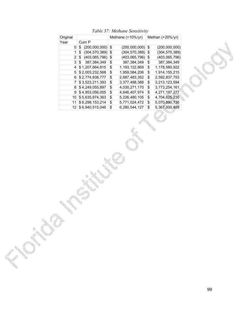
99

Table 37: Methane Sensitivity

Original Methane (+10%/yr) Methan (+20%/yr)

Year Cum P

0 (200,000,000)$ (200,000,000)$ (200,000,000)$

1 (304,570,389)$ (304,570,389)$ (304,570,389)$

2 (403,065,796)$ (403,065,796)$ (403,065,796)$

3 387,384,349$ 387,384,349$ 387,384,349$

4 1,207,664,815$ 1,193,122,869$ 1,178,580,922$

5 2,003,232,568$ 1,959,584,206$ 1,914,155,215$

6 2,774,838,777$ 2,687,483,352$ 2,592,837,753$

7 3,523,211,393$ 3,377,498,388$ 3,213,123,594$

8 4,249,055,897$ 4,030,271,170$ 3,773,254,161$

9 4,953,056,005$ 4,646,407,974$ 4,271,197,277$

10 5,635,874,363$ 5,226,480,105$ 4,704,625,235$

11 6,298,153,214$ 5,771,024,472$ 5,070,890,736$

12 6,940,515,046$ 6,280,544,127$ 5,367,000,489$

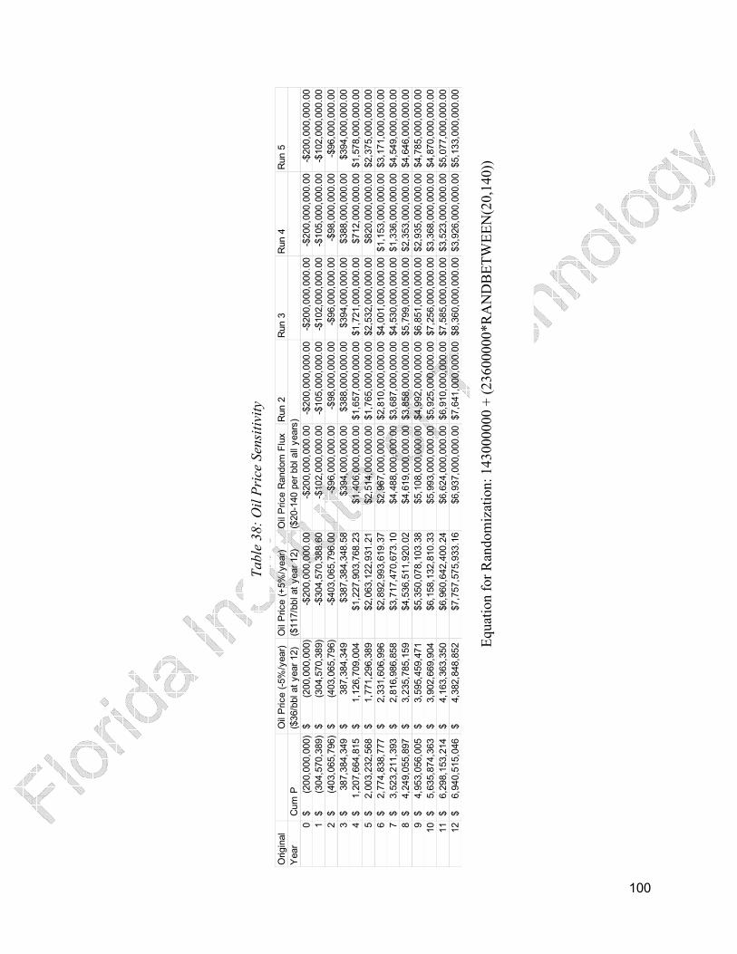
100

Origin

al

Oil

Price (

-5%

/year)

Oil

Price (

+5%

/year)

Oil

Price R

andom

Flu

xR

un 2

Run 3

Run 4

Run 5

Year

Cum

P($

36/b

bl at

year

12)

($117/b

bl at

year

12)

($20-1

40 p

er

bbl all

years

)

0(2

00,0

00,0

00)

$

(2

00,0

00,0

00)

$

-$200,0

00,0

00.0

0-$

200,0

00,0

00.0

0-$

200,0

00,0

00.0

0-$

200,0

00,0

00.0

0-$

200,0

00,0

00.0

0-$

200,0

00,0

00.0

0

1(3

04,5

70,3

89)

$

(3

04,5

70,3

89)

$

-$304,5

70,3

88.6

0-$

102,0

00,0

00.0

0-$

105,0

00,0

00.0

0-$

102,0

00,0

00.0

0-$

105,0

00,0

00.0

0-$

102,0

00,0

00.0

0

2(4

03,0

65,7

96)

$

(4

03,0

65,7

96)

$

-$403,0

65,7

96.0

0-$

96,0

00,0

00.0

0-$

98,0

00,0

00.0

0-$

96,0

00,0

00.0

0-$

98,0

00,0

00.0

0-$

96,0

00,0

00.0

0

3387,3

84,3

49

$

387,3

84,3

49

$

$387,3

84,3

48.5

8$394,0

00,0

00.0

0$388,0

00,0

00.0

0$394,0

00,0

00.0

0$388,0

00,0

00.0

0$394,0

00,0

00.0

0

41,2

07,6

64,8

15

$

1,1

26,7

09,0

04

$

$1,2

27,9

03,7

68.2

3$1,4

06,0

00,0

00.0

0$1,6

57,0

00,0

00.0

0$1,7

21,0

00,0

00.0

0$712,0

00,0

00.0

0$1,5

78,0

00,0

00.0

0

52,0

03,2

32,5

68

$

1,7

71,2

96,3

89

$

$2,0

63,1

22,9

31.2

1$2,5

14,0

00,0

00.0

0$1,7

65,0

00,0

00.0

0$2,5

32,0

00,0

00.0

0$820,0

00,0

00.0

0$2,3

75,0

00,0

00.0

0

62,7

74,8

38,7

77

$

2,3

31,6

06,9

96

$

$2,8

92,9

93,6

19.3

7$2,9

67,0

00,0

00.0

0$2,8

10,0

00,0

00.0

0$4,0

01,0

00,0

00.0

0$1,1

53,0

00,0

00.0

0$3,1

71,0

00,0

00.0

0

73,5

23,2

11,3

93

$

2,8

16,9

86,8

58

$

$3,7

17,4

70,6

73.1

0$4,4

88,0

00,0

00.0

0$3,6

87,0

00,0

00.0

0$4,5

30,0

00,0

00.0

0$1,3

36,0

00,0

00.0

0$4,5

49,0

00,0

00.0

0

84,2

49,0

55,8

97

$

3,2

35,7

85,1

59

$

$4,5

36,5

11,9

20.0

2$4,6

19,0

00,0

00.0

0$3,8

58,0

00,0

00.0

0$5,7

99,0

00,0

00.0

0$2,3

53,0

00,0

00.0

0$4,6

46,0

00,0

00.0

0

94,9

53,0

56,0

05

$

3,5

95,4

59,4

71

$

$5,3

50,0

78,1

03.3

8$5,1

08,0

00,0

00.0

0$4,9

92,0

00,0

00.0

0$6,8

51,0

00,0

00.0

0$2,9

35,0

00,0

00.0

0$4,7

85,0

00,0

00.0

0

10

5,6

35,8

74,3

63

$

3,9

02,6

69,9

04

$

$6,1

58,1

32,8

10.3

3$5,9

93,0

00,0

00.0

0$5,9

25,0

00,0

00.0

0$7,2

56,0

00,0

00.0

0$3,3

68,0

00,0

00.0

0$4,8

70,0

00,0

00.0

0

11

6,2

98,1

53,2

14

$

4,1

63,3

63,3

50

$

$6,9

60,6

42,4

00.2

4$6,6

24,0

00,0

00.0

0$6,9

10,0

00,0

00.0

0$7,5

85,0

00,0

00.0

0$3,5

23,0

00,0

00.0

0$5,0

77,0

00,0

00.0

0

12

6,9

40,5

15,0

46

$

4,3

82,8

48,8

52

$

$7,7

57,5

75,9

33.1

6$6,9

37,0

00,0

00.0

0$7,6

41,0

00,0

00.0

0$8,3

60,0

00,0

00.0

0$3,9

26,0

00,0

00.0

0$5,1

33,0

00,0

00.0

0

Table

38:

Oil

Pri

ce S

ensi

tivi

ty

Equat

ion f

or

Ran

dom

izat

ion:

143000000 +

(23600000*R

AN

DB

ET

WE

EN

(20,1

40))

101

Appendix E: Literature Review

With advancements in directional drilling technology, new methods of extraction omit

much of the danger and manual labor associated with strip mining. These new methods involve

drilling horizontal wells into bitumen formations deep underground into which high pressure

steam and sometimes other lubricants and extraction aids liquefy the semi-solid carbon

formations. The slurry is then pumped above ground where it can be converted into desirable

compounds. A popular version of this extraction method is called Steam Assisted Gravity

Drainage (SAGD), which takes advantage of Earth’s gravity to allow newly liquefied bitumen in

an upper well to move downward to a secondary well awaiting transfer to the surface by pump.

An advantage of SAGD-type extraction is that the well effluent typically has a more consistent

concentration and the injection and extraction pump forces do not interfere with one another

wasting energy.

Other drilling methods are similar to SAGD. CSS, or Cyclic Steam Stimulation, also uses

steam to reduce the viscosity of the bitumen and enable it to be pumped out of the ground. Steam

is injected periodically, allowing the steam to “soak” and infiltrate the surrounding areas, and

then the bitumen is pumped up to the surface. This requires only one borehole, while SAGD

requires two (one to inject the steam, one to recover the bitumen). In addition, CSS uses “wet”

steam, containing both vapor and hot water, while SAGD uses only “dry” steam. High Pressure

Cyclic Steam Stimulation (HPCSS) also uses wet steam, but by injecting the steam at a high

pressure it fractures the surrounding areas, which allows the bitumen to flow. This can be

problematic, as sometimes where it flows to is not able to be completely controlled. In Primrose

South, in Canada, this became such a problem that low pressure steam was needed to be used

instead (Noaman, 2013).

102

Steam flooding, in contrast, utilizes two vertical boreholes. One pipe “floods” the area

with steam that moves towards the other borehole and reduces the viscosity of the surrounding

bitumen, which is pumped out of the second borehole. This process is simpler to execute than the

other methods, as no horizontal drilling is necessary.

If the bitumen deposit is of the proper type, CSS is one of the best methods to extract the

bitumen, since it works on a greater range of sediments, in and around the reservoir bed,

allowing for recovery rates of 25 to 30 percent of the entire bed (not just the steam chamber

area). However, in the Athabasca area, where this plant is proposed to be built, the oil sands

deposit is shallower and has no capping formation (Lui, 2006). Therefore SAGD is the most

viable method.

Table 39: Overview of Bitumen Extraction Processes

SAGD CSS HPCSS Steam Flooding

Steam Type Dry Wet Wet Wet

Boreholes 2 1 1 2

Bitumen

/Reservoir

Type

High Conc. Bitumen, high viscosity

Less viscous bitumen

Thinner inter-bedded

reservoirs

Heavy oil, high viscosity

Direction Horizontal Usually Horizontal

Either Vertical

Method Gravity drainage Gravity drainage, Re-compaction drive, solution

gas drive

Fracturing Physical Displacement

Considerations Must have high bitumen saturation in

soil, good for reservoirs with top gas or bottom water

Must have capping shale,

allows for use in broader range of reservoir quality

Containment issues, lower recovery than

SAGD

Cannot be used below 5000 ft. due

to sediment pressure

(Lui, 2006) (Glacier, 2002) (Bioage, 2013) (Noaman, 2013)

103

Other extraction methods are also possible, although significantly less utilized. For

example, VAPEX (Vapor Extraction), ET-DSP (Electro-Thermal Dynamic Stripping Process),

and ISC (In Situ Combustion). These use a variety of methods (vaporized solvents, additional

heating via electricity or burning some of the oil, etc.) to reduce the viscosity of the bitumen

enough for pumping (Calgary, 2014).

The water for the steam for SAGD is often taken from local sources, but an increasing

trend is to draw from ground water tables deemed unsuitable for consumption so as to avoid

interfering with surface water. A significant portion of the water is also drawn from byproduct

and recycle streams from further along the process. Any residual wastewater from processes

such as blowdown is re-injected deep underground (Pembina, 2010).

The water used for steam passes through a series of pumps and boilers to establish the

necessary temperature and pressure to travel underground and deliver the necessary heat to

decrease the viscosity of the bitumen. Research using alternate media for the process has been

conducted, but with little success given the process is much more reliant on heat transfer than it

is on solvency. For example, while supercritical CO2 can prove to be an effective solvent to the

bitumen hydrocarbons, the cost of delivering supercritical CO2 in volumes necessary to liquefy

and dissolve the heavy oils for extraction exceeds that of delivering the high pressure steam

which is able to liquefy the hydrocarbon mixture in less volume due to its much higher heat

capacity.

When a well is activated, a significant portion of steam hosted energy is lost to the

overburden and underburden as the ground itself is heated around the well. At start up, energy

losses can top out at 70% of injection enthalpy, causing a lower than predicted retrieval rate (Oil,

2010). This rate picks up as the well process temperatures reach steady state with the

104

surrounding earth, which can take several months depending on the properties of the surrounding

burden. The target for heat losses is generally 50% or lower (2010).

The terminology “synthetic” in synthetic crude oil refers to the crude being,

“synthetically constructed as a mixture of several component hydrocarbon streams, each of

which are produced and then blended at a production facility” (Sundram, 2013).

Separation Processes

Once pumped to the surface, the bitumen, water, and sediment mixture is fed to a settler.

A solvent is added, typically either naphtha or a paraffinic solvent, depending on the water

content of the bitumen (Alberta, 2015). As the extraction process is steam-based, it can be

assumed that the bitumen has the higher water content, so the solvent for this design will be

naphtha. Since one of the products of the plant (before being combined into synthetic crude) is

naphtha, some of this stream can be used as the solvent in the settler. The solvent separates the

bitumen from the water into a bitumen froth, which is allowed to float to the top and is therefore

separated. Naphtha is nonpolar, similar to the hydrocarbon chains in bitumen. It then works as an

effective solvent to separate the bitumen hydrocarbons from the polar water molecules.

As for further separation, two vacuum distillation columns will be used to separate bitumen

and later the reacted bitumen into streams based on ranges of molecular weights. Vacuum

distillation is chosen as it significantly reduces the amount of coke formed and thus is often

chosen for separation (Vacuum 2009) (Eurobitume 2014). The vacuum can be achieved through

use of a steam ejector (2009), but pumps are also often utilized. Since a pump is easier to model

as it is a separate piece of equipment, this was the chosen method.

105

Catalyst Characteristics

One of the biggest complications involved in the hydrocracking and hydrotreating

processes when upgrading bitumen hydrocarbons is the exorbitant variety in feed components.

While most all components in the feed are chemically similar, they are not equal. It can be

assumed no single catalyst would be equally efficient in facilitating these reactions among all

components. This is why in hydrocarbon hydroprocessing, reactors typically use a mixture of

several catalysts at some ratio to match the predicted feed composition. For our simulation, we

intended to cut down the feed variety by assuming a composition of only a set of the most

prominent components typically found in Athabasca bitumen based on literature. This would

have simplified the simulation of the process in Aspen, and would also have allowed us to come

to a conclusion on the catalyst mixture required. However, this simplification was too basic and

did not capture enough of the behavior of the bitumen.

In the textbook “Hydroprocessing of Heavy Oils and Residua,” James Speight outlines a

series of conditions the ideal hydroprocessing catalyst must satisfy; low cost, no adverse effect

from regeneration processes, stability in microcrystalline phases, stability of corresponding

sulfide compounds drawn from feed, high purity, support site inactivity with feedstock, thermal

stability under operating conditions, and the ability to form a multitude of shapes with high

mechanical strength. Matching all of these criteria, [gamma]-Alumina tends to be the

predominant choice (Speight, 2007). The [gamma]-Alumina acts as a support to deliver Cobalt,

Vanadium, Molybdenum, and Nickel oxides and sulfides to the feed which also aid the cracking

and treating processes. Given the majority of the catalyst is [gamma]-Alumina, it may be

reasonable to assume the entirety of the catalyst media is [gamma]-Alumina.

The catalyst mixture acts by providing both acidic and basic sites to encourage release of

carbon-carbon bonds and carbon-N/O/S/M bonds, “cracking” or “treating,” in the presence of

106

hydrogen gas. When the carbon bonds break, a highly unstable carbocation forms and begins a

chain reaction with itself or other local molecules, rearranging rapidly, until recombination or

bonding with a free radical. In the high pressure and temperature, with an abundance of

hydrogen, reverse reactions are suppressed forcing the adoption of hydrogen atoms to stabilize

the carbon chains; while sulfur, nitrogen, oxygen, and metals tend to almost immediately form

their respective hydrides, H2S, NH3, H2O, and HM. Metal hydrides are far less common, but

build up in the catalyst bed along with undesired cokes.

Ferric sulfate was decided to be the best catalyst for this particular process. It is very

cheap (Alibaba 2015), it lasts longer than some other catalyst types, trace metals such as

vanadium and nickel (Bhattacharjee, 2010) are caught in it during the reaction processes, and it

can be regenerated (Peck, 1941).

Hydrocracking and hydrotreating are essentially the same reaction, but are named

differently to differentiate them each from their primary goals. Hydrocracking, which occurs at a

much higher pressure and temperature, seeks to exclusively break carbon-carbon bonds at a

conversion rate typically around 50%, while the lower pressure and temperature hydrotreatment

seeks to conserve carbon structure and only remove undesired groups from the chains at a

conversion rate of 10-20% (Jechura, 2014). Their catalysts are nearly identical, but as mentioned

have their compositions tailored to fit their specific feed stock. Given that Aspen cannot

simulate catalyst activity directly, assumptions could be made on their make-up for the purpose

of costing, but exact compositions for each reactor may not be necessary to satisfy simulation.

At a later date closer to plant construction, experiments may be performed to discover the exact

mix required to optimize reactor performance and conversion.

107

Reactor

Literature shows that a SCO yield of about 80wt% can be achieved for a coking-based

scheme for the same operating conditions. In contrast, the hydroconversion-based upgrading

scheme generates a SCO yield of about 90wt%. The difference in the SCO yield between the two

schemes is due to the fact that the ebullated bed hydroconversion unit completely converts the

vacuum bottoms into gaseous and liquid products without generating any solid residual material.

The SCO from hydroconversion-based scheme has slightly lower concentrations of sulfur,

nitrogen and aromatics than that from coking-based scheme. This results from the

hydrodesulphurization, hydrodenitrogenation and hydrogenation, in addition to the

hydrocracking of heavy molecules, occurring in the ebullated bed hydrocracker. The

hydroconversion-based upgrading scheme has a higher SCO yield at the cost of higher hydrogen

consumption. (Munteanu, 2012)

Safety and Environmental Concerns

Compared to traditional coking, hydroconversion uses substantially less water, using less

than 17% of the water coking uses (Munteanu, 2012). Additional water and energy savings can

be found by the use of SAGD as opposed to other extraction methods. The once-steam

generators (heaters) used to make the steam typically generate 75 % steam and 25% hot water

(Lui, 2006). Since SAGD requires dry steam only, the water can be recovered for use in the

reactors. The water coming out of the hydrotreaters can also be recycled.

However, since there is a significant amount of steam required for any of the steam

extraction techniques the necessary energy input is fairly high. Several processes reviewed

burned natural gas as the heat input, which generates a lot of CO2, much more than traditional

bitumen extraction methods (Nuwer, 2013). However, there is the possibility to do CO2

sequestration in the steam injection stream.

108

Although this process isn’t using any solvents in the steam, if they were to be used it

would allow for the possibility of chemical seepage into the water table or atmosphere. Since the

SAGD is pulling material from the ground, it can create void spaces which can destabilize

ground layers. Once a drilling operation ceases for a given reservoir, the mine can be reclaimed

by reintroducing the sand and related materials into the mine (EIS, 2012).

As for safety concerns, hydrogen sulfide gas can be dangerous to breathe if allowed to

reach certain concentrations. It is also highly corrosive. Symptoms include nausea, headaches,

etc., up to death depending on the concentration and length of exposure (OSHA, 2014). It can

also be explosive depending on concentration (2014). Ammonia is also highly corrosive and can

cause lung damage if inhaled in sufficient concentrations. As the SAGD gas will be highly

pressurized and at high temperature, precautions must be taken and PPE must be worn. This is

true for many if not all of the other processes, including near the reactors. The bitumen itself is a

skin irritant and studies differ on whether it is carcinogenic (Wess, 2005). Since the reactors deal

in high pressures and temperatures, properly sized relief and rupture valves will need to be fitted.

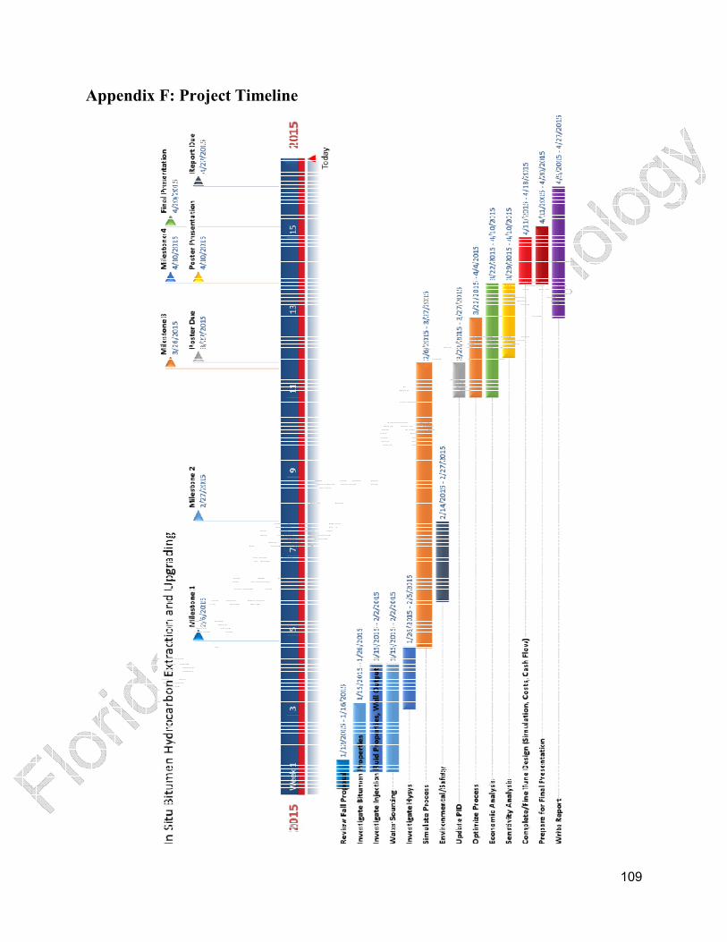
109

Appendix F: Project Timeline