CHE Research Paper 10 - York

Income, Relative Income, and Self-Reported Health in Britain 1979-2000

CHE Research Paper 10

Income, relative income, and self-reported health in Britain 1979-2000

Hugh Gravelle∗ Matt Sutton+ March 2006 ∗ National Primary Care Research and Development Centre, Centre for Health Economics, University of York, York, YO10 5DD. Email: [email protected] + Health Economics Research Unit, University of Aberdeen, Foresterhill, Aberdeen, AB25 2ZD. Email: [email protected]

Background CHE Discussion Papers (DPs) began publication in 1983 as a means of making current research material more widely available to health economists and other potential users. So as to speed up the dissemination process, papers were originally published by CHE and distributed by post to a worldwide readership. The new CHE Research Paper series takes over that function and provides access to current research output via web-based publication, although hard copy will continue to be available (but subject to charge). Acknowledgements Funding from the Department of Health to NPCRDC and from the Chief Scientist Office to HERU is acknowledged. The views expressed are those of the authors and not necessarily those of the funders. Helpful comments were made by Ken Judge, and John Wildman, and by participants in the Glasgow July 2004 meeting of the Health Economists’ Study Group, and the York Seminars in Health Econometrics. Disclaimer Papers published in the CHE Research Paper (RP) series are intended as a contribution to current research. Work and ideas reported in RPs may not always represent the final position and as such may sometimes need to be treated as work in progress. The material and views expressed in RPs are solely those of the authors and should not be interpreted as representing the collective views of CHE research staff or their research funders. Further copies Copies of this paper are freely available to download from the CHE website www.york.ac.uk/inst/che/pubs. Access to downloaded material is provided on the understanding that it is intended for personal use. Copies of downloaded papers may be distributed to third-parties subject to the proviso that the CHE publication source is properly acknowledged and that such distribution is not subject to any payment. Printed copies are available on request at a charge of £5.00 per copy. Please contact the CHE Publications Office, email [email protected], telephone 01904 321458 for further details.

Centre for Health Economics Alcuin College University of York York, UK www.york.ac.uk/inst/che

© Hugh Gravelle, Matt Sutton

Abstract According to the relative income hypothesis, an individual’s health depends on the distribution of income in a reference group, as well as on the income of the individual. We use data on 231,208 individuals in Great Britain from 19 rounds of the General Household Survey between 1979 and 2000 to test alternative specifications of the hypothesis with different measures of relative income, national and regional reference groups, and two measures of self assessed health. All models include individual education, social class, housing tenure, age, gender and income. The estimated effects of relative income measures are usually weaker with regional reference groups and in models with time trends. There is little evidence for an independent effect of the Gini coefficient once time trends are allowed for. Deprivation relative to mean income and the Hey-Lambert-Yitzhaki measures of relative deprivation are generally negatively associated with individual health, though most such models do not perform better on the Bayesian Information Criterion than models without relative income. The only model which performs better than the model without relative income and which has a positive estimated effect of absolute income on health has relative deprivation measured as income proportional to mean income. In this model the increase in the probability of good health from a ceteris paribus reduction in relative deprivation from the upper quartile to zero is 0.010, whereas as an increase in income from the lower to the upper quartile increases the probability by 0.056. Measures of relative deprivation constructed by comparing individual income with incomes within a regional or national reference group will always be highly correlated with individual income, making identification of the separate effects of income and relative deprivation problematic. Keywords: relative income, relative deprivation, income inequality, health. JEL numbers: I12, I31.

Income, relative income, and self-reported health in Britain 1979-2000 1

1. Introduction There is considerable evidence that individuals with higher incomes have better health (see for example, Pritchett and Summers, 1997) but that the beneficial effects of income decline with income (see for example, Ettner, 1996). It has also been suggested that an individual’s health is affected by the income of other individuals in a reference group (Wilkinson, 1996; Marmot, 2004). The relative income hypothesis takes a variety of forms (Deaton, 2003; Wagstaff and van Doorslaer, 2000). One strand in the literature (the income inequality hypothesis) focuses on the overall distribution of income and suggests that an individual in a society with greater income inequality will have worse health, even if they have the same income as an individual in a more egalitarian society. It is suggested that societies with greater income inequality may have patterns of public and private consumption which reduce health, for example they may invest less in public health (Lynch et al, 2000). Another strand (the relative deprivation hypothesis) suggests that what matters is the difference between an individual’s income and the incomes of individuals in their reference group, rather than overall inequality in income distribution. Here the emphasis is on psychosocial explanations: relative deprivation induces stress and anxiety which lead to physical ill health (Marmot and Wilkinson, 2001). Most of the empirical literature attempting to test the relative income hypothesis has used aggregate level data and looked for a relationship between population health, mean income and measures of income inequality. The majority of the aggregate level analyses suggest that, holding per capita income constant, population health is worse in societies with less equal income distributions (see the studies surveyed in Deaton, 2003; Lynch et al, 2004; Judge and Paterson, 2001; Mellor and Milyo, 2001; Wagstaff and van Doorslaer, 2000; Wilkinson and Pickett, 2006). A substantial minority of aggregate level studies find no or a positive relationship between population health and income distribution (for example Gravelle, Wildman and Sutton, 2001; Mellor and Milyo, 2001; Muller, 2002; Ross et al, 2000). Aggregate level studies are attempts to test the income inequality version of the relative income hypothesis. Such aggregate level analyses cannot test relative deprivation hypotheses as this requires measures of individuals’ incomes relative to some reference group. Nor can they test the plausible suggestion that the effects of income inequality or of relative deprivation differ across richer and poorer individuals. Aggregate studies also suffer from an obvious aggregation problem: in general it is impossible to test hypotheses about individual level relationships with data averaged over individuals unless the relationships are linear. If income improves health but at a decreasing rate, increases in the dispersion of income will reduce mean health, even if the health of an individual is entirely determined by their own income (Rodgers, 1979; Gravelle, 1998). Studies with data on health and income linked at individual level are on the whole less favourable to simple versions of the relative income hypothesis (Mackenbach, 2002). Some studies find no relationship between income inequality and health (eg Blakely, Atkinson and O’Dea (2003)), or that income inequality is positively associated with health (eg Osler, Christensen, Due et al, 2003; Chang and Christakis, 2005). But others find a negative association (eg Diaz-Roux, Link and Northridge, 2000; Subramanian and Kawachi, 2006.). There have been four individual level studies using British data. Craig (2005) used two years of the Scottish Household Survey and reported that individual self assessed health is better for individuals in local authorities with higher Gini coefficients after allowing for individual gender, age, income, education, economic status and Local Authority mean income. The other three UK studies are based on the British Household Panel Survey (BHPS). Weich, Jenkins and Lewis (2002) used the first, 1991, wave of the BHPS and found some evidence of a detrimental effect of income distribution on self reported health with the effect being more pronounced amongst poorer individuals. The relationship was not robust to the measure of income distribution, being strongest for the Gini coefficient. They noted that income inequality is greater in more urban regions and suggest that income inequality may be picking up some characteristic of cities. Weich, Lewis and Jenkins (2001) looked at mental health, measured using the General Health Questionnaire, in the first wave of BHPS. Individuals with the lowest incomes had the worst mental

2 CHE Research Paper 10

health, but higher income individuals had worse mental health than those on moderate incomes. For individuals with low incomes, mental health problems were more common if they lived in regions with low Gini coefficients, whereas for individuals with high incomes they were more common in those living in regions with high Gini coefficients. Thus income inequality had an adverse effect on the mental health of the rich and a protective effect for the poor. Wildman and Jones (2002) also used the BHPS but with panel data methods to allow for unobserved individual heterogeneity. They found that mental health was unrelated to income but was adversely affected by subjective measures of financial well-being. The mental health of poor women was adversely affected by the Hey and Lambert (1980) and Yitzhaki (1979) relative deprivation measure (see section 3.3) but men and those on higher incomes were not affected. The implication of these UK studies is that the association between income inequality and health is sensitive to the measures of health, of income, and of income distribution. They also suggest that the association may be different for the rich and the poor. In this paper we make a number of contributions. First, we use data from 19 rounds of the British General Household Survey (GHS). Although the sample of individuals was different in each round of the GHS, so that we are unable to allow for individual unobservable heterogeneity, there are considerable compensations in using the GHS. In addition to a large sample size in each period, the data span a period (1979 from 2000) which experienced upturns and downturns in the economic cycle and varying changes in the economic fortunes of different regions within Britain and considerable changes in the degree of income inequality (Goodman and Shephard, 2002). Second, we compare four variants of the relative income hypothesis: one version of the income inequality hypothesis using the Gini coefficient and three versions of the relative deprivation hypothesis. Third, we test if the effects of relative income differ for individuals with below and above average income. Fourth, in modeling the effect of relative deprivation on health it is not obvious a priori what population is the relevant reference group. The estimated effect of relative deprivation has been found to vary with the reference group used to construct income inequality or relative deprivation measures (Osler, Christensen, Due et al, 2003). With our data set we are able to use both national and regional reference groups in constructing our measures of income inequality and relative deprivation. Finally, we use a three category general health measure and a binary measure of functioning (absence of limiting long term illness) to examine the sensitivity of results to the health measure.


2. Data 2.1 General Household Survey Data on individual health and household income are from the General Household Survey (GHS) which is a representative cross section survey of private households in England, Scotland and Wales (www.statistics.gov.uk/ssd/surveys/general_household_survey.asp). We use 19 annual cross-sections from the period 1979-2000/1:1 there was no GHS in 1997 and 1999 and we had to drop the 1983 round because neither the income variable nor the variables required to calculate it were available in the public-use dataset. Summary statistics for the sample used in the analysis are in Table 1. Table 1. Summary statistics Variable Cases Mean St.Dev. Min Max Age (years/100) 231208 0.4146 0.1485 0.1700 0.6900 Female 231208 0.5248 No long term limiting illness 231208 0.8067 ‘Good’ self-assessed health 231208 0.6399 ‘Fairly Good’ self-assessed health 231208 0.2539 ‘Not Good’ self-assessed health 231208 0.1062 Equivalised income yijt 231208 0.1596 0.0996 0.0000 1.0000 Annual mean income yt 19 0.1444 0.0195 0.1172 0.1785 Annual Gini coefficient Gt 19 0.3290 0.0359 0.2687 0.4051

Annual additive relative deprivation A1 231208 0.0424 0.0339 0.0000 0.1785

Annual additive relative affluence A2 231208 0.0576 0.0719 0.0000 0.8215

Annual proportional relative deprivation R1 231208 0.2891 0.2201 0.0000 1.0000

Annual proportional relative affluence R2 231208 0.3936 0.4693 0.0000 4.6011 Annual income ratio yijt/yt 231208 1.1045 0.6463 0.0000 5.6011 Regional year mean income yjt 209 0.1445 0.0258 0.1033 0.2146 Regional year Gini coefficient Gjt 209 0.3228 0.0377 0.2516 0.4501

Regional year additive relative deprivation A1 231208 0.0414 0.0343 0.0000 0.2144

Regional year additive relative affluence A2 231208 0.0565 0.0702 0.0000 0.8541

Regional year proportional relative deprivation R1 231208 0.2827 0.2188 0.0000 1.0000

Regional year proportional relative affluence R2 231208 0.3861 0.4558 0.0000 5.8529 Regional year income ratio yijt/yjt 231208 1.1034 0.6314 0.0000 6.8529 Owns home 231208 0.6580 Rents home 231208 0.3420 High formal qualifications 231208 0.0993 Medium formal qualifications 231208 0.2791 Low formal qualifications 231208 0.2035 Foreign/other qualifications 231208 0.0289 No formal qualifications 231208 0.3893 Social class I 231208 0.0380 Social class II 231208 0.1896 Social class IIINM 231208 0.2691 Social class IIIM 231208 0.2151 Social class IV 231208 0.1922 Social class V 231208 0.0665 Social class: unclassified. 231208 0.0294

1 Each round of the GHS was initially administered within a calendar year but from 1988/89 onwards rounds took place within financial years.


The main advantage of the GHS for our purposes is the long time-period covered. We are restricted to variables that have been collected consistently throughout the period and use two self-reported simple measure of health status, gross household income, age, gender and information on educational attainment, housing tenure and social class. Educational information is available only for respondents aged less than 70. Self-assessed health status is asked only of respondents aged 16 and over. We therefore use only the 16-69 age group. We measure the age variable as age in years/100. The measure of household income that has been collected throughout the period is gross household income, before tax and housing costs. Income has been converted to 2000 prices using the Retail Price Index (Office for National Statistics, 2003a). In all years household income has been equivalised using the Before Housing Costs McClements scale (Office for National Statistics, 2003b). The equivalised income variable is linearly transformed so that the minimum value = 0 and the maximum value = 1. Information on income and self-assessed health is available for 241,779 individuals (73.4% of the initial sample of 16-69 year olds. We omit the 1st and 99th percentiles of the income distribution to remove zero incomes and some very large reported incomes, since these may have disproportionate effects on the estimated income-health relationship and measures of relative income. There is also missing information for some respondents on home ownership, education level and social class. The resulting sample size is 231,208 (70.2%). Reference groups were created by stratifying the sample by (a) year only and (b) year and eleven areas (Scotland, Wales and 9 English regions). Measures of income inequality within reference groups and reference group mean incomes were based on all respondents with non-missing and non-outlier income information as they are most likely to be representative of the reference groups. In the region-within-year analyses observations are distributed across 209 strata (11 regions over 19 years). The median and inter-quartile range of the strata size are 1,028 and 791-1,256. One of the reasons suggested for the fact that US studies are more likely to find an effect of relative income is that income inequality is greater in the US than in other countries studied and has greater variation across US states and over time than between and within other countries. In our data the yearly Ginis range from 0.27 to 0.41 and the region-within-year Ginis from 0.25 to 0.45, variations that are comparable with those observed in the US.

2.2 Health measures

We use two health measures. The first is a three-category measure of self-assessed general health status and the second is the absence of a chronic condition which limits the individual’s daily functioning. Increases in both measures correspond to better health. Self-assessed health measures have been shown to be good predictors of subsequent mortality (Idler and Benyammi, 1997) for all socio-economic groups (Burström and Fredlund, 2001) and to be strongly associated with mortality rates at local authority level (Kyfinn, Goldacre, Gill et al, 2004). 2.2.1 General health Self-assessed general health status (SAH) is derived from answers to the question “How would you rate your health in general? Good, fairly good or not good”. It is a widely used measure and was, for example, part of the UK’s decennial population census in 2001. We used STATA 8.2 [oprobit, robust cluster(group)] to estimate ordered probit models of individual level general health. We use robust standard errors and allow for clustering of the error terms between respondents in the same region and year. The specification of the health regression varies according to the form of the relative income hypothesis. 2.2.2 Absence of limiting long standing illness (ALLI) The GHS also contains the question “Do you have any long-standing illness, disability or infirmity? By long-standing, I mean anything that has troubled you over a period of time or that is likely to affect you


over a period of time?” Those who report a longstanding illness are then asked if it limits their activities in any way. To make comparison with the results from the general health measure easier we define a binary health measure taking the value 1 if the individual does not report limiting longstanding illness and 0 otherwise. We estimate the resulting individual model as a logistic regression [probit, robust cluster(group)].

3. Specifications of the relative income hypothesis

3.1 Income inequality The first set of models test for an effect of income inequality as measured by the Gini coefficient G on health. The Gini is frequently used in the literature, especially in aggregate level studies. When the reference group is the national population the model is

2 3 40 1 2 3 4 1ijt ijt ijt ijt ijt t ijt ijth y y y y G x uβ β β β β γ δ′= + + + + + + + (1)

where hijt is the latent health measure for individual i in region j in year t, yijt is equivalised household income, ijtx′ is a vector of demographic and socio-economic individual variables. The power function of income here and in the other specifications allows for the non-linearity of the relationship between income and health. We estimate a number of variants of (1). (a) We allow for the possibility that the effect of the Gini depends on whether the individual is “rich” (income above the reference group mean) or “poor” (income below reference group mean) by adding a term t

ijt tD G where the dummy variable ( tijtD )

indicates whether the individual has income below or above the national average yt in that year ( 1=t

ijtD if ijt ty y≤ ; = 0 otherwise). (b) We also estimate (1), and all the other specifications discussed below, with the reference group being the region, so that the mean income level for defining the “poor” dummy is the mean income in region j in year t ( 1=jt

ijtD if ijt jty y≤ ; = 0 otherwise) and Gt is replaced by Gjt (and analogously in the other specifications below). (c) Although we do not show them in (1) or in the other equations describing our models, we also allow for regional effects by the inclusion of region dummies with the South East of England as the baseline region. In models with regional reference groups we also incorporate year dummies with 1979 as the baseline year. In models with national reference groups, year dummy variables would be perfectly collinear with variables like the national Gini coefficient which are invariant across individuals within a year. Hence national reference group models do not contain year dummy variables. However, we do separately examine the relationship between national Ginis and the year effects from a model estimated without national Ginis and estimate a model where the time trend is modeled as a linear effect. (d) It is plausible that reported health is determined by previous values of income and relative income (Benzeval and Judge, 2001). Since the GHS is a cross section and contains current data on individuals we cannot allow for possible lagged effects of socioeconomic factors on health. However we can calculate measures of income distribution for previous years and we estimate specifications with the current year Gini plus the Ginis for the previous five years. (e) Osler, Christensen, Due et al (2003) found some evidence that the effect of income distribution was non-linear. We therefore also consider specifications with quadratic and cubic functions of the Gini.


3.2 Deprivation relative to mean income

The second variation of the relative income hypothesis is that individuals have worse health the higher the mean income of their reference group.2 To save notational clutter we write the model in terms of the conditional expected value of the individual’s health, suppress the individual, region and year subscripts and collect the higher powers of income and socio-economic variables and any year and region effects into the constant term: 0 1 1 2( ) ( )h y y z D y zβ β λ λ= + + − + − (2) where h is now the conditional expected value of individual health, y is individual income, z is the mean income of the reference group and D = 1 if y z≤ and 0 otherwise.3 If 01 >λ an increase in the mean income reduces the health of someone with a given income above the mean. An increase in mean income reduces the health of a person with a given income below the mean if 021 >+ λλ .

Mean income has a greater impact on the poor if 02 >λ .4 The measure of relative deprivation in (2) is additive since y z− is unaffected by adding a constant to the income of the individual and all those in her reference group. Thus an individual with an income of £10,000 whose reference group has a mean income of £20,000 faces the same relative deprivation as in individual with an income of £40,000 whose reference group has a mean income of £50,000. We also investigate specifications in which health depends on the proportionate difference

/y z between individual income and the reference group mean income so that /y z replaces y z− in (2).

3.3 Relative deprivation

The use of mean income as the comparator implies that an individual with an income of 2 units would feel as deprived in a society with an income distribution (2,2,3,3,3,3) as in an economy with distribution (1,2,2,2,2,7). Measures of relative deprivation which are sensitive to the whole distribution of income rather than its mean, and which allow for the possibility that health is differentially affected by the income distribution above and below the individual’s income, can be derived as follows (Yitzhaki, 1979; Hey and Lambert, 1980; Deaton, 2003). Define the extent of additive relative deprivation for an individual with income y with respect to another individual in her reference group with income z as

( )1 ; if0 if

a y z z y z yz y

= − ≥

= < (3)

Letting f(z) denote the relative frequency of income in the reference group, and F(y) the cumulative relative frequency, the total additive relative deprivation experienced by an individual with income y with respect to all individuals in the reference group is

( )1 1( ) ; ( ) ( ) ( )y y

A y a y z f z dz z y f z dz∞ ∞

= = −∫ ∫ (4)

2 There is an obvious link with the literature on life and job satisfaction where investigators have found that satisfaction of individuals is lower the higher the income of a reference group (Clark and Oswald, 1996; Ferrer-i-Carboneli, 2002). 3 The estimated models contain the full set of income powers, socio-economic variables and year and region effects as appropriate. 4 We also specified the model as 0 1 2 3 4h y Dy z Dzβ θ θ θ θ= + + + + , where 1 1 1θ β λ= + , 2 2θ λ= , 4 2θ λ= − and

found that we could not reject the null that the two estimates of the differential effect on the poor ( 2λ ) were equal:

2 4ˆ ˆ 0θ θ+ = .


which is decreasing and convex in the individual’s income:

1 1( ) [1 ( )] 0, ( ) 0A y F y A f y′ ′′= − − < = > (5) It is also possible that an individual may care about being richer than other individuals. Define her additive relative affluence (relative satisfaction in Yitzhaki (1979)) with respect to an individual with income z as

( )2 ; if0 if

a y z y z y zy z

= − ≥

= < (6)

and her total additive relative affluence as

( )2 2 10 0( ) ; ( ) ( ) ( ) ( ) ( )

y yA y a y z f z dz z y f z dz A y z y= = − − = − −∫ ∫ (7)

which is increasing and convex in own income. The relative deprivation measures have the advantage of being individual rather than reference group specific, so we are able to include year effects even when we use national reference groups. We allow both additive relative deprivation and additive relative affluence to affect health:

0 1 1 1 2 2( ) ( )h y A y A yβ β ψ ψ= + + + (8) So that health is reduced by relative deprivation if 1ψ < 0 and increased by relative affluence if

2 0ψ > . Using (7) we see that (8) nests the case in which only income relative to the mean has a

detrimental effect on health ( 1 2 0ψ ψ+ = , 1 0ψ < ). Relative deprivation and affluence may also be measured so that equiproportional changes in income have no effect on how relatively deprived the individual feels. Replacing a1(y,z) and a2(y,z) in the definitions of additive relative deprivation and affluence by 1( , ) /a y z z and 2 ( , ) /a y z z gives

proportional relative deprivation and affluence as 1 1( ) ( ) /R y A y z= and 2 2( ) ( ) /R y A y z= which are dimensionless and lie in [0,1]. We estimate specifications with both proportional relative deprivation and affluence

0 1 1 1 2 2( ) ( )h y R y R yβ β φ φ= + + + (9) which also nests the special case in which only income proportional to mean affects health ( 1 1 20, 0φ φ φ< + = ). 3.4 Magnitude of relative deprivation effect We gauge the importance of the estimated effects of relative deprivation by comparing them with the effects of other covariates such as region of residence, income, education, housing tenure and social class. We examine the effect of changing, one at a time, each of these variables on the probability of being in good self-assessed health for a baseline individual: male; aged 42 years; in rented accommodation; with no formal qualifications; in social class V; living in the North West of England in 2000/1; income at the lower quartile. We change the categorical variables from the baseline ‘bottom’ to the ‘top’ category. For example, we calculate the change in probability of good health of changing the education variable from ‘No formal qualifications’ to ‘High formal qualifications’ holding all other variables at their baseline values. We measure the magnitude of the effect of income by comparing


the probability of good self-assessed health for an individual with the same characteristics as our baseline individual but a level of income at the upper quartile. We assign our baseline individual the upper quartile of relative deprivation for the set of individuals with a similar income level. By ‘similar income’ we mean the 185 individuals whose income is within 0.0001 of the income of our baseline individual. (Remember that income is normalised to lie between 0 and 1.) We estimate the effects of reducing relative deprivation holding all other variables constant, including income. First, we calculate the probability of good self-assessed health for an individual with the same characteristics as the baseline individual but the lower quartile of relative deprivation for the individuals with similar incomes. Second, we calculate this probability for an individual with baseline characteristics but no experience of relative deprivation, i.e. where all individuals have incomes at the lower quartile. 4. Results Given the number of different models, most non-nested, we compare models using a version of the Bayesian Information Criterion (BIC′) which adjusts the log-likelihood for the number of observations and regressors (Raftery, 1996). The more negative the BIC′ the better the model.5 Raftery (1996) suggests that when the absolute value of the difference between the BIC′ scores for two models is less than 2 there is only weak evidence in favour of the model with the more negative BIC′ but that an absolute difference of over 10 is very strong evidence in favour of it. In each table the most negative BIC′ is in bold font. For the relative income models which perform better than the model with no relative income effects we also check that the estimated effect of absolute income is positive. 4.1 Models with no relative income effects Table 2 shows the results from the ordered probit regression of self-assessed health (SAH) and the probit regression of absence of limiting longstanding illness (ALLI) on year and region dummies and all the individual level demographic and socio-economic variables, except measures of relative income or deprivation. The coefficients show the effects of the variables on the conditional mean of the underlying latent health index so that a positive coefficient indicates that an increase in the variable shifts the distribution to the right and increases the conditional mean of the latent health index. We will therefore refer, a little loosely, to variables increasing or decreasing SAH or ALLI. The results for the two health measures are qualitatively similar and plausible. We have omitted the age and gender variables from Table 2 to save space. For men SAH declines with age over the range (20, 69) whilst ALLI declines over the entire age range (17, 69). For women SAH declines over the range (20, 66) and ALLI declines over the range (17, 65). 5% of women were aged over 66. For both measures women are healthier than men at all ages. Individuals living in rented accommodation are less healthy and there are clear gradients of health with education and social class: the better educated and those in higher social classes are healthier. Note however that the negative effect of worse education on ALLI is statistically significant only for no formal qualifications compared with high formal qualifications. Income is standardised to lie between 0 and 1. Over the income range (0.00, 0.89) SAH is increasing with income, steeply up to 0.25 and then more slowly. Over the income range (0.90, 1.00) health decreases with income, although only 0.02% of the sample have incomes in this range. Increases in income increase ALLI over the ranges (0.0, 0.98), though there is little effect over the range (0.25, 0.60). Over a range of income covering the vast majority of the population, income has a positive and diminishing effect on latent health.

5 BIC′ = BIC + 2*ln Likelihood (Intercept only) + (N-1)*ln (N), where BIC = –2*ln Likelihood(Model) – (N – (K+1))*ln(N), K is number of regressors in the model and N the number of observations. The difference between BIC′ for models with the same N is equal to the difference between BIC. We use BIC′ because it is has fewer digits than BIC and hence is easier to compare across models.


Table 2. Determinants of self assessed health: no relative income effects

General self assessed health

(SAH) Absence of long term limiting

illness (ALLI)

Coeff. z Coeff. z

Rents home -0.221 -34.2 -0.189 -22.4

Medium formal qualifications -0.110 -9.2 -0.026 -1.6

Low formal qualifications -0.166 -13.8 -0.026 -1.7

Foreign/other qualifications -0.207 -10.7 -0.031 -1.3

No formal qualifications -0.283 -23.5 -0.087 -5.3

Social class II -0.052 -3.1 -0.077 -3.8

Social class IIINM -0.069 -4.0 -0.082 -3.9

Social class IIIM -0.148 -8.5 -0.129 -6.2

Social class IV -0.160 -8.8 -0.130 -6.4

Social class V -0.168 -9.3 -0.120 -5.3

Social class unclassified. -0.116 -5.0 -0.228 -8.2

Equivalised income 4.490 12.6 5.343 11.8

Equivalised income2 -11.619 -5.9 -15.575 -6.0

Equivalised income3 13.466 3.5 19.124 3.6

Equivalised income4 -5.609 -2.4 -7.935 -2.4

North of England -0.104 -6.0 -0.104 -5.4

Yorkshire/Humberside -0.090 -7.1 -0.074 -5.7

North West England -0.119 -12.7 -0.106 -8.4

East Midlands -0.048 -4.4 -0.027 -2.0

West Midlands -0.065 -6.3 -0.035 -2.4

East Anglia 0.040 2.4 0.019 1.1

London -0.080 -5.8 -0.054 -3.4

South West England 0.046 3.8 -0.011 -0.7

Wales -0.075 -6.1 -0.158 -11.8

Scotland 0.001 0.1 -0.007 -0.5

1980 -0.053 -3.5 -0.080 -3.6

1981 0.039 3.0 -0.026 -1.3

1982 0.038 2.4 -0.043 -1.7

1984 0.043 2.4 -0.036 -1.3

1985 0.021 1.3 -0.058 -2.3

1986 -0.041 -2.8 -0.143 -5.7

1987 -0.101 -7.4 -0.231 -9.2

1988/89 -0.118 -7.0 -0.174 -7.0

1989/90 -0.066 -3.7 -0.136 -5.9

1990/91 -0.127 -7.2 -0.263 -12.2

1991/92 -0.047 -2.5 -0.115 -5.1

1992/93 -0.070 -4.4 -0.149 -6.2

1993/94 -0.098 -8.1 -0.236 -9.8

1994/95 -0.119 -5.2 -0.185 -6.6

1995/96 -0.148 -11.2 -0.191 -7.9

1996/97 -0.233 -12.6 -0.328 -14.1

1998/99 -0.202 -11.9 -0.234 -10.3

2000/01 -0.211 -11.5 -0.162 -5.8

Log-Likelihood (Initial) -201576.36 -113518.97

Log-Likelihood (Model) -188343.68 -103234.69

Pseudo-R2 0.0656 0.0906

BIC’ -25847.8 -19951.0

Observations (N) 231,208 231,208 Reference group: owns home, high formal qualifications, social classs I, South East England, 1979. Models also contain age, age2, age3, gender and gender*age, gender*age2, gender*age3. BIC’ = BIC + 2*ln Likelihood (Intercept only) + (N-1)*ln (N), where BIC = - 2*ln Likelihood(Model) – (N-(K+1))*ln(N), K is number of regressors in the model, and N the number of observations. z = coefficient/standard error.


There are significant unexplained area effects on health (South East England is the omitted area). For SAH the best areas are South West England, East Anglia, and Scotland and the three worst are Yorkshire and Humberside, Northern England and North West England. For ALLI, East Anglia, South East England and Scotland are the best, and Northern England, North West England and Wales the worst, areas. The year coefficients for both health measures are plotted in Figure 1 and suggest a secular, though not monotonic, decline in health over the period.

1979 1984 1989 1994 1999

Year

Year

Effe

cts

SAH ALLI

Figure 1. Year effects from models with no relative income effects The addition of measures of relative income to the health regressions had little effect on the coefficients of the non-income variables and the partial effects of relative income were qualitatively very similar for the two health measures. We therefore report in Table 2 to 6 just the coefficients on the relative income measures from the regression of SAH on a full set of covariates. For some of the models the coefficients on the four powers of income were affected by the addition of relative income and we note in the text when the partial effect of income is changed materially. 4.2 Income inequality The results in Table 3 are for various specifications of the income inequality version of the relative income model. All the models include regional dummies, except where stated. Consider first the results with national reference groups (models 7 to 12). When the reference group is the national population and we do not include a time trend or year dummies (models 7, 9, 11, 12), increases in the Gini are associated with worse SAH in most of the specifications. The coefficient on the Gini is negative and highly significant, whether or not we include regional dummies. When the national Gini is allowed to have a different effect for individuals with above and below mean income (model 11), its effect is significantly more negative for the poor. In the lagged model (model 12), the effects of the two most recent years national Ginis are negative and the effect of a given increase in the national Gini


Table 3. Tests of the income inequality hypothesis: effect of Gini coefficient on self assessed health

Regional reference group National reference group Year

effects Coef. z BIC′ Year

effects Coef. z BIC′

1. G No -1.60 -11.20 -25597.6 7 No -1.76 -13.27 -25674.3 2. G Yes 0.94 3.40 -25847.1 8 Trend 1.33 3.02 -25793.9 3. G no regional effects No -1.63 -9.59 -25377.7 9 No -1.73 -9.43 -25262.8 4. G no regional effects Yes -0.77 -2.36 -25561.1 10 Trend 1.30 1.9 -25377.7 5. G Yes 0.97 3.49 -25845.2 11 No -1.65 -11.60 -25668.5 G*D -0.10 -2.93 -0.08 -2.30 6. G Yes 0.98 1.55 12 No -5.40 -2.5 G-1 -0.75 -1.24 -12.30 -2.9 G-2 0.05 0.07 7.25 2.0 G-3 0.62 0.97 12.29 5.5 G-4 0.23 0.34 20.28 4.1 G-5 -0.50 -0.81 -24.87 -6.6

Negative coefficient indicates that relative deprivation worsens health. Dependent variable: self assessed health. Ordered probit regression. All models include individual characteristics and regional effects unless stated otherwise G: Gini. G-t: Gini at lag t years. D: dummy for income below mean. BIC′ = BIC + 2*ln Likelihood (Intercept only) + (N-1)*ln (N), where BIC = - 2*ln Likelihood(Model) – (N—(K+1))*ln(N) and K is number of regressors in the model. z = coefficient/standard error.


sustained over five years is also negative. In the quadratic specification (not shown) increases in the Gini increase health but in the cubic specification (not shown) increases in the Gini reduce SAH.6 The results for the national reference group are strongly affected by the inclusion of a linear time trend in models 8 and 10: the coefficients on national Gini becomes positive. The reason is that, as Table 2 and Figure 1 show, there is a downward trend in SAH when no relative income terms are included in the health equation. The national Gini has a strong upward trend over the period. Hence in the national Gini models with no time trend, where we cannot include year dummies because of perfect collinearity, the Gini picks up the downward health trend. Including a linear time trend leaves the national Gini to explain variations around the trend and its coefficient becomes positive. Figure 2 is a scatter plot of the year effects from the first model in Table 2 (where we do not include any relative income variables) against the year Ginis. The national Gini is highly negatively correlated (R2 = 0.620) with the year effects.

-0.25

-0.2

-0.15

-0.1

-0.05

0

0.05

0.1

0.2 0.25 0.3 0.35 0.4 0.45

Gini coefficient

Year

effe

cts

(SA

H)

Figure 2. SAH year effects and year Ginis

The significance of the national Gini in the health models is not necessarily due to a causal effect. Any national level variable which is trended over time would also have a significant effect in the health model. Moreover, when two time series are trended the correlation between them can be entirely spurious. Figure 3 plots the first differences of the year effects against the first differences of the year Gini. The R2 is just 0.006, and here there is no evidence that the Gini affects health. The results with regional year reference groups (models 1 to 6) provide little support for the income inequality version of the relative income hypothesis. When year dummies are included (models 2, 4, 5, 6) the effects of the regional-year Gini are positive for both health measures, both for individuals with above and below average income. The coefficients for the quadratic and cubic models (not

6 In the quadratic model SAH is increasing when the Gini is greater than 0.20. (The minimum observed national Gini is 0.27.) In the cubic model SAH decreases with the Gini over the range (0.29, 0.40).


shown) are insignificant and SAH is increasing in the regional Gini.7 All the coefficients on the lagged Ginis in model 6 are insignificant.

-0.12

-0.08

-0.04

0

0.04

0.08

0.12

-0.02 -0.01 0 0.01 0.02 0.03 0.04 0.05 0.06

First differenced Gini coefficients

Firs

t diff

eren

ced

year

effe

cts

(SA

H)

Figure 3. SAH year effects and year Ginis: first differences

Dropping the year effects from the models with regional-year Ginis leads to the coefficient on the Gini becoming negative and significant (models 1, 3), irrespective of whether regional effects are also included. The reason is that the regional Ginis are correlated with unobserved regional year effects. We ran an ordered probit regression of general self assessed health on the individual level variables plus region, year, and region by year dummy variables, with no relative income measures. Figure 4 plots the coefficients on the region by year dummies against the region by year Ginis and shows that they are weakly negatively correlated (R2 = 0.0049). For models with regional-year or year Ginis as the measure of relative income the estimated effect of the Gini depends crucially on whether the models include variables (a set of year dummies or a time trend) which capture the downward trend in self reported health. In models where we include both Ginis and such temporal variables, the coefficient on the Gini suggests no or even a positive effect of income inequality on health. Models with area and year effects (or a time trend) perform better (by the BIC′) than those without them. The best performing model (2) has year effects and a regional reference group and has a positive effect of the Gini on health. But all of the Gini models in Table 3 (and models with powers of the Gini) perform worse than the models without any relative income effects (Table 2).

7 For the quadratic model SAH is increasing in the Gini for values of the Gini above 0.22. The minimum regional Gini is 0.25. In the cubic model SAH increases over the entire range [0,1] for which Ginis are defined.


-0.3

-0.2

-0.1

0

0.1

0.2

0.3

0.2 0.25 0.3 0.35 0.4 0.45 0.5

Gini coefficient

Reg

ion

by y

ear e

ffect

s (S

AH

)

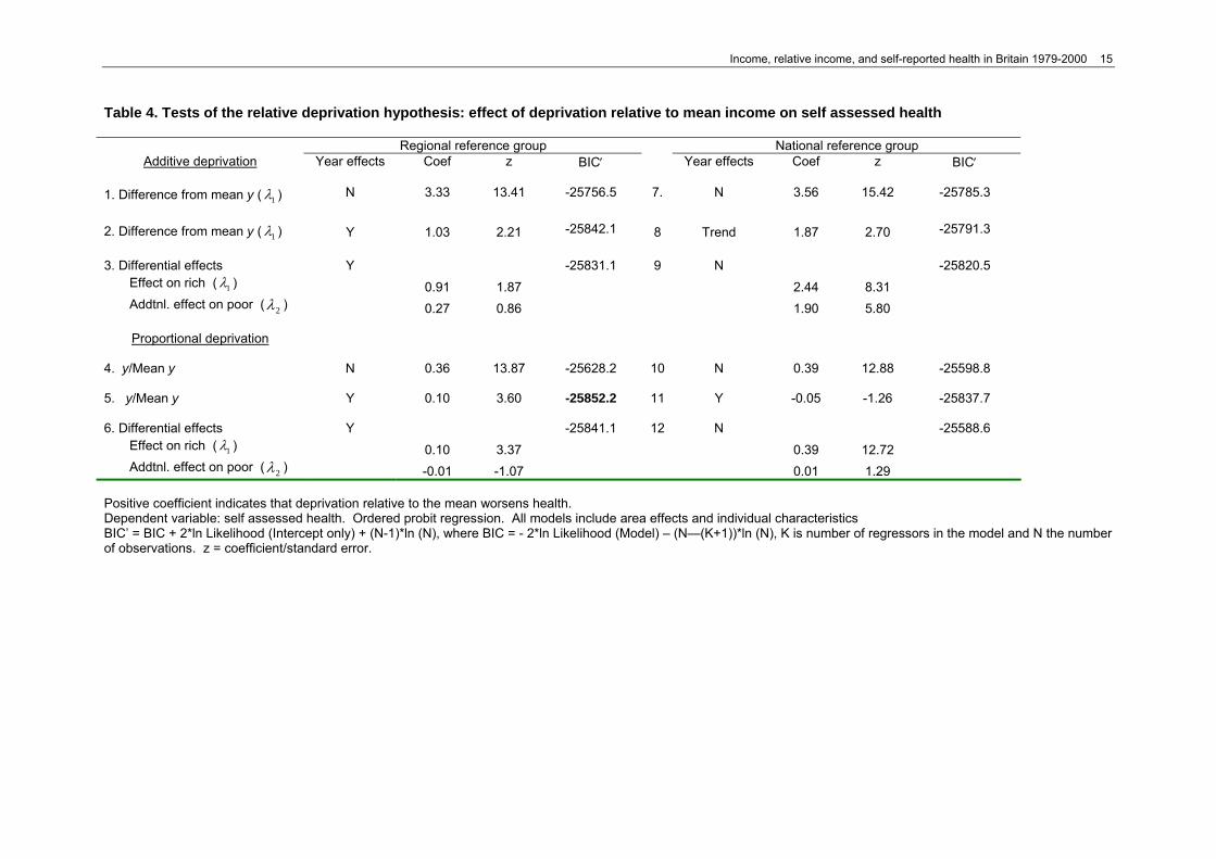
Figure 4. SAH Region-Year effects and Ginis 4.3 Deprivation relative to mean income In the models in Table 4 relative income is defined as the (absolute or proportional) difference between the individual’s income and the mean of a reference group. Referring back to the health equation (2), relative deprivation reduces health if 1λ is positive (so decreases in income relative to the mean reduce health). In all but one of the models increases in income relative to the mean improve health. Models with a time trend or year effects again perform better (by the BIC′) than those without and regional reference group models perform better than the equivalent models with national reference groups. In only one of the models (9) is the effect on those with below mean incomes significantly greater than the effect on those with income above mean. The best performing model (5) has deprivation measured proportionately to the mean of the regional reference group. It is the only model in Table 4 that performs better than the SAH model in Table 2 with no relative deprivation variables. However, while increases in relative deprivation reduce health significantly, the estimated income coefficients imply that latent health is increasing in income up to income of 0.28 and then decreasing for the remainder of the income range which covers 10.8% of the sample.


Table 4. Tests of the relative deprivation hypothesis: effect of deprivation relative to mean income on self assessed health

Regional reference group National reference group Additive deprivation Year effects Coef z BIC′ Year effects Coef z BIC′

1. Difference from mean y ( 1λ ) N 3.33 13.41 -25756.5 7. N 3.56 15.42 -25785.3

2. Difference from mean y ( 1λ ) Y 1.03 2.21 -25842.1 8 Trend 1.87 2.70 -25791.3

3. Differential effects Y -25831.1 9 N -25820.5 Effect on rich ( 1λ ) 0.91 1.87 2.44 8.31

Addtnl. effect on poor ( 2λ ) 0.27 0.86 1.90 5.80

Proportional deprivation 4. y/Mean y N 0.36 13.87 -25628.2 10 N 0.39 12.88 -25598.8 5. y/Mean y Y 0.10 3.60 -25852.2 11 Y -0.05 -1.26 -25837.7

6. Differential effects Y -25841.1 12 N -25588.6 Effect on rich ( 1λ ) 0.10 3.37 0.39 12.72

Addtnl. effect on poor ( 2λ ) -0.01 -1.07 0.01 1.29

Positive coefficient indicates that deprivation relative to the mean worsens health. Dependent variable: self assessed health. Ordered probit regression. All models include area effects and individual characteristics BIC’ = BIC + 2*ln Likelihood (Intercept only) + (N-1)*ln (N), where BIC = - 2*ln Likelihood (Model) – (N—(K+1))*ln (N), K is number of regressors in the model and N the number of observations. z = coefficient/standard error.


4.4 Relative deprivation Tables 5 and 6 reports results from models with the Hey-Lambert-Yitzhaki measures of relative deprivation and affluence. Allowing for time trends makes a considerable difference to the results. The coefficient on A1 is negative and has large z statistics when there are no year effects (models 1, 7). With year effects (models 2, 6) the coefficients are greatly reduced in size and significance and become positive and insignificant in the regional reference group model (2). With the proportional relative deprivation measure R1, the use of year effects again greatly reduces the magnitude and significance of the coefficients on R1 (compare models 4, 10 against 5, 11), though the coefficients are negative and remain significant even for the regional reference groups. When we attempt to test for the effects of both additive relative deprivation and affluence with a regional reference group (model 3), the effect of additive relative affluence is positive and significant but the effect of additive relative deprivation is insignificant. With national reference groups (model 9) additive relative deprivation has a significant negative effect and the effect of additive relative affluence is small and insignificant. With the regional reference group, but not with the national reference group, we would reject the null hypothesis that only income relative to the mean affects health at the 5% significance level. Proportional relative deprivation has a highly significant negative effect and proportional relative affluence a marginally statistically significant positive effect with regional reference groups (model 6). But with a national reference group (model 12), whilst proportional relative deprivation has a statistically significant negative coefficient, proportional relative affluence has a statistically significant negative effect. We reject the null hypothesis that only income proportional to the mean affects health for both reference groups, though the rejection is much stronger for the national reference group. Comparison of the BIC′ scores suggest that models with national reference groups perform better than those with regional reference groups and those with proportional relative deprivation do better than those with additive relative deprivation. Three of the models (6, 11, 12) in Table 5 perform better than the SAH model with no relative deprivation measure. The best is model 11, which has a negative effect of proportional relative deprivation measured against the national reference group. However, model 11 has individually insignificant coefficients on the powers of individual income and latent health decreases with income over the entire range. Model 12, with a national reference group, has a significant negative effect of relative deprivation and a negative but insignificant effect of relative affluence but latent health is decreasing in income up to income of 0.15 and for income between 0.48 to 0.72, ranges which account for 59.8% of observations. Model 6, with a regional reference group, has a significant negative effect of relative deprivation and a positive and significant effect of relative affluence. It also a range of income over which latent health is decreasing in income: 0.20 to 0.89 which has 24.0% of the observations. Table 6 reports models with powers of the relative deprivation measures. As with Table 5, models with national reference groups and using proportional relative deprivation have better BIC′ scores than those with regional reference groups and using additive relative deprivation. All the models with powers of relative deprivation have better BIC′ scores than the model without relative deprivation in Table 2 and the best performing model is cubic in proportional relative deprivation with a national reference group. However, all the models in Table 6 have at least one unappealing feature: insignificant coefficients on income powers; health decreasing over some ranges of income; or health increasing over some ranges of the relative deprivation measures. For example, the cubic models (3, 6, 9, 12) have health increasing with relative deprivation over some ranges. The problem is more severe with proportional relative deprivation: in model 12 health is increasing in R1 for R1 ≤ 0.34 and R1 ≥ 0.45 ranges with the national reference group (which contain 88.7% of the observations). For the regional reference group model 6, health is increasing in R1 for R1 ≤ 0.33 and R1 ≥ 0.41, ranges which contain 91.4% of the observations. Both the quadratic regional reference group models (2, 5) and the national quadratic additive relative deprivation model 8 have health increasing over some ranges of the relative deprivation measures. The quadratic models with national reference groups (2, 11) have insignificant coefficients on the income powers.


Table 5. Tests of the relative deprivation hypothesis: effect of additive and proportional relative deprivation on self assessed health

Regional reference group National reference group Additive deprivation Year effects Coef z BIC′ Year effects Coef z BIC′

1. Relative deprivation (A1) N -3.47 -12.58 -25626.9 7 N -4.17 -15.75 -25768.7 2. Relative deprivation (A1) Y 0.39 0.89 -25836.7 8 Y -1.84 -2.75 -25845.7

3. Relative deprivation and affluence: Y -25837.9 9 Time trend -25796.0 Effect of relative deprivation 1ψ

-0.56 -1.08

-2.23 -2.99

Effect of relative affluence 2ψ . 1.72 3.24

1.00 1.23

Ho: only income proportional to mean affects health 1 2 0ψ ψ+ =

χ2(1)= 5.53 p=0.0187 χ2(1)= 3.07 p<0.0800

Proportional deprivation 4. Relative deprivation (R1) N -0.94 -14.33 -25711.1 10 N -1.00 -14.72 -25770.6 5. Relative deprivation (R1) Y -0.26 -1.96 -25841.8 11 Y -0.72 -4.18 -25862.2 6. Relative deprivation and affluence: Y -25849.1 12 Y -25849.9 Effect of relative deprivation 1φ

-0.43 -3.19

-0.69 -3.50

Effect of relative affluence 2φ 0.11 3.90

-0.01 -0.29

Ho: only income proportional to mean affects health 1 2 0φ φ+ =

χ2(1)= 5.98 p=0.0145 χ2(1)= 15.44 p=0.0001

Negative coefficient indicates that relative deprivation worsens health. Dependent variable self assessed health. Ordered probit regression. All models include area effects and individual characteristics. BIC’ = BIC + 2*ln Likelihood (Intercept only) + (N-1)*ln (N), where BIC = - 2*ln Likelihood(Model) – (N-(K+1))*ln(N) and K is number of regressors in the model. z = coefficient/standard error.


Table 6. Effect of powers of additive and proportional relative deprivation on self assessed health

Regional reference group National reference group Coef z BIC′ Coef Z BIC′ Additive relative deprivation 1. Linear -25836.7 7 -25845.7 A1 0.39 0.89 -1.84 -2.75 2. Quadratic -25873.3 8 -25894.3 A1 -3.34 -4.41 -8.02 -7.48 A1 squared 16.82 6.34 24.60 7.28 3. Cubic -25873.7 9 -25944.3 A1 -0.61 -0.55 3.43 1.87 A1 squared -16.86 -1.31 -89.47 -5.48 A1 cubed 139.51 2.52 489.95 6.97 Proportional relative deprivation 4. Linear -25841.8 10 -25862.2 R1 -0.26 -1.96 -0.72 -4.18 5. Quadratic -25880.8 11 -25871.8 R1 -0.67 -5.05 -0.99 -5.55 R1 squared 0.56 6.2 0.39 4.13 6. Cubic -26030.4 12 -26070.6 R1 1.41 6.17 1.97 7.04 R1 squared -3.87 -9.09 -5.05 -11.94 R1 cubed 3.49 10.77 4.24 13.13

Negative coefficient indicates that relative deprivation worsens health. Ordered probit regression. All models include area and year effects, and individual characteristics. BIC’ = BIC + 2*ln Likelihood (Intercept only) + (N-1)*ln (N), where BIC = - 2*ln Likelihood(Model) – (N-(K+1))*ln(N), K is number of regressors in the model and N the number of observations. z = coefficient/standard error.


These examples are illustrations of a major difficulty in attempting to test for relative deprivation versions of the relative income hypothesis: an individual’s relative deprivation is a decreasing non-linear function of their income. But income also plausibly has a direct positive and non-linear effect on their health. If the relative deprivation measures are highly correlated with income, any regression equation which includes them both is likely to suffer from severe multi-collinearity. It will be difficult to identify the separate effects of income and relative deprivation since standard errors will be increased, and coefficient estimates will be highly sensitive to the set of observations used to estimate them. We also regressed the relative deprivation measures on all the individual variables, year dummies and regional dummies. The R2 for the four (regional, year, additive, proportional) regressions ranged between 0.9521 and 0.9925. The variance inflation factors ranged between 20.9 and 133.3. There is more independent variation in the additive compared to the proportional measures, and in the regional compared to the year measures, but in all cases the variance inflation factors are large enough to suggest serious multi-collinearity. The condition indices (Greene, 2000, pp. 255-259) for the four relative deprivation measures ranged from 951.7 to 953.2. Condition indices over 20 are usually regarded as a cause for concern. 4.5 Importance of the relative deprivation effect We calculated the importance of the estimated relative deprivation effects for two models. The first uses the income proportional to the regional mean specification (Table 4, model 5, BIC’ = -25852), which was the best performing example of this type and has a positive effect of income on health. The second uses the additive relative deprivation specification with a national reference group and year effects (Table 5, model 8, BIC’ = -25711), which has the best (most negative) BIC′ for this type of model amongst those with positive effects of income on health. The results are in Table 7. Consider first the calculations for the model with relative deprivation measured as income proportional to the regional mean. The probability of good health for the baseline individual is 0.445. In the baseline scenario, the baseline individual has income at the lower quartile (0.088) and this income is 56% of his regional mean. At the upper quartile of the distribution of relative deprivation for individuals with a similar income, the income is 76% of regional mean income. Setting the level of relative deprivation experienced by the baseline individual, to 0.76 whilst holding all other variables including their income constant, increases the probability of good health to 0.453. Removing relative deprivation completely, by setting the ratio of the baseline individual’s income to the regional mean to one, yields a predicted probability of 0.463. The increases in the probability of good health due to the reduction or elimination of relative deprivation are substantially smaller than those for the changes in the other covariates. Increasing his income to the upper quartile or moving his location to the South East of England (holding all other factors constant, including relative deprivation) results in a good health probability of 0.50. The largest increases in good health probability are associated with changes in education and housing tenure. Table 7. Effects of relative deprivation on estimated probabilities of good self assessed health compared with effects of other variables

Specification of relative deprivation measure Scenario Ratio of income to mean income

– regional reference group Additive relative deprivation –

national reference group Baseline 0.445 0.451 Relative deprivation at lower quartile 0.453 0.480 All individuals with same income 0.463 0.510 Income at upper quartile 0.501 0.504 High formal qualifications 0.557 0.564 Social class I 0.511 0.518 Owns home 0.533 0.539 S.E. England 0.503 0.499 The baseline scenario refers to a male; aged 42 years; in rented accommodation; with no formal qualifications; in social class V; living in the North West of England in 2000/1; a level of income at the lower quartile; and a level of relative deprivation at the upper quartile of the group of individuals with this level of income.


The second set of results in Table 7 are based on the model with additive relative deprivation measured relative to a national reference group. The estimated impact of relative deprivation is larger, though the model performs less well overall than the one underlying the first set of results. Reducing the baseline individual’s relative deprivation from the upper quartile (0.081) to the lower quartile (0.041), halves his relative deprivation and increases the probability of good health from 0.451 to 0.480. Eradicating relative deprivation entirely results in a further increase in the probability of good health to 0.510. This is smaller than the estimated effects of education, social class and home ownership but larger than the effects of region of residence and an increase in the individual’s income from the lower quartile to the upper quartile. 5. Conclusions 5.1 Summary of results The qualitative results were unaffected by whether the health variable was the three category measure of general self assessed health or the binary absence of limiting longstanding illness. We used two types of measures of relative income. The first is a measure of overall income inequality (the Gini) which varies by year when the reference group is national, or by year and region when the reference group is regional. Income inequality increased over the period and self assessed health decreased. In models with national Ginis and no time trend, the coefficient on the Gini was negative and significant, but in models with a time trend the coefficient on the Gini was positive and significant. Similarly, adding regional dummies to models with regional Ginis changed the coefficient on the Gini from negative to positive. The Bayesian Information Criterion suggests that the models including Gini coefficients perform worse than models without them. The results provide no support for a negative effect of income inequality as measured by the Gini on health in Britain. The second type of relative income measures varies by individual. When relative deprivation is measured as the ratio of income to the reference group mean income, most of the models indicate that relative deprivation worsens health. But only one of them, with relative income measured as income proportional to the region-in-year mean income, performs better, in terms of the Bayesian Information Criterion, than a model with no relative deprivation measures. The effect of this measure of relative deprivation on the probability of good health is small compared to changes in income, education, social class or housing type. When the Hey-Lambert-Yitzhaki relative deprivation measure is used, increases in relative deprivation are generally associated with worse health, and three of the twelve models considered perform better than the model with no relative deprivation. But these three models do not have significant positive estimated effects of income on health. Models with powers of the Hey-Lambert-Yitzhaki measure perform better than the linear models but have health either decreasing with income over non-trivial ranges of income or increasing with relative deprivation over non-trivial ranges of relative deprivation. Our best performing relative income model which has sensible estimated effects on income uses national reference groups to construct the Hey-Lambert-Yitzhaki proportional relative deprivation measure. The negative effects of the measure on the probability of good health are smaller than those of own income, education, social class, and region. Moreover, the model performs worse than a model with no relative income measure. 5.2 Discussion Our analyses do not yield any strong evidence in favour of the relative income hypothesis. Even with multi-level data, there are two principal problems in identifying an effect of relative income on the health of individuals. First, there are likely to be missing variables which affect health and whose means vary over time and across areas. If measures of income inequality are defined at area and year level they may pick up the effects of the missing variables in addition to any true effect of income inequality. We found that adding area and time dummies markedly reduced the size of the effect of income inequality and sometimes changed its sign. The problem is less severe for individual level measures of relative deprivation which depend on the income of an individual as well as on the distribution of income in an area or year. In the case of the HLY measures of relative deprivation, for example, we can allow for secular trends in health even with national reference groups. But ideally,


we require a sufficiently rich set of variables so that region and year dummies are insignificant in the individual level health models; the relative deprivation measures must then reflect only the effects of relative deprivation, rather than being contaminated by unobserved factors operating at the level of the regional or year reference groups. Second, relative deprivation measures are derived from the individual’s income as well as the income distribution of a reference group. They are by construction highly correlated with individual income unless there are substantial differences in the income distributions of the reference group for individuals on similar incomes. Our data set exhibited considerable variation in income distributions over time and across regions. The fact that we found very high multi-collinearity between individual incomes and measures of relative deprivation suggests that attempts to test for relative income effects on data sets that contain no direct information on reference groups and relative income are unlikely to be fruitful. A solution might be to ask individuals directly if they feel themselves to be relatively deprived, or to ask them about their reference groups. But if individuals choose their reference groups and their choices are affected by their incomes or their health, such data will not produce reliable estimates of the effects of relative deprivation on health unless coupled with models of reference group choice and the data to identify them. We are rather pessimistic about whether any data set will permit identification of relative deprivation effects.


References Benzeval, M., Judge, K., 2001. Income and health: the time dimension. Soc Sci Med 52, 1371-1390. Blakely, T., Atkinson, J., O’Dea, D., 2003. No association of income inequality with adult mortality

within New Zealand: a multi-level study of 1.4 million 25-64 year olds. J Epidemiol Community Health 57, 279-284.

Burström, B., Fredlund, P., 2001. Self rated health: Is it as good a predictor of subsequent mortality among adults in lower as well as in higher social classes? J Epidemiol Community Health 55, 836-840.

Chang, V.W., Christakis, N.A. 2005. Income inequality and weight status in US metropolitan areas. Soc Sci Med, 61, 83-96.

Clark, A., Oswald, A., 1996. Satisfaction and comparison incomes. Journal of Public Economics 61, 359-381.

Craig, N., 2005. Exploring the generalisability of the association between income inequality and self-assessed health. Soc Sci Med 60, 2477-2488.

Deaton, A., 2003. Health, inequality, and economic development. Journal of Economic Literature 41, 113-158.

Diaz-Roux, A.V., Link, B.G., Northridge, M.E., 2000. A multilevel analysis of income inequality and cardiovascular disease. Soc Sci Med 50, 673-687.

Ettner, S.L., 1996. New evidence on the relationship between income and health. Journal of Health Economics 15, 67-85.

Ferrer-i-Carboneli, A., 2002. Income and well-being: an empirical analysis of the comparison income effect. Tinbergen Institute Discussion Paper TI 2002-019/3, http://www.tinbergen.nl

Goodman, A., Shephard, A., 2002. Inequality and living standards in Great Britain: some facts. Briefing Note 19. Institute for Fiscal Studies, London.

Gravelle, H., 1998. How much of the relationship between population mortality and inequality is a statistical artefact? BMJ 316, 382-385.

Gravelle, H., Wildman, J., Sutton, M. 2001. Income, income inequality and health: what can we learn from aggregate data? Soc Sci Med 54, 577-589.

Greene, W.H., 2000. Econometric Analysis, 4th Edition, Prentice Hall, London. Hey, J.D., Lambert, P.J. 1980. Relative deprivation and the Gini coefficient: comment. Quarterly

Journal of Economics 94, 557-573. Idler, E.L., Benyammi, Y., 1997. Self-rated health and mortality: a review of twenty-seven community

studies. J Health Soc Behav 38, 21-37. Judge, K., Paterson, I., 2001. Poverty, income inequality and health. Treasury Working Paper 1/29

http:/www.treasury.govt.nz/workingpapers/2001/twp01-29.pdf Kyffin, R.G.E., Goldacre, M.J., Gill, M., 2004. Mortality rates and self reported health: database

analysis by English local authority area. BMJ 329, 887-888. Lynch, J.W., Davey-Smith, G., Harper, S., Hillemeier, M., 2004. Is income inequality a determinant of

population health. Part 1. A systematic review. The Milbank Quarterly 82, Lynch, J.W., Davey-Smith, G., Kaplan, G.A., House, J.S., 2000. Income inequality and mortality:

importance to health of individual incomes, psychosocial environment, or material conditions. BMJ 320, 1200-1204.

Mackenbach, J.P., 2002. Income inequality and population health. BMJ 324, 1-2. Marmot, M., 2004. Status Syndrome. How Social Standing Directly Affects Your Health and Life

Expectancy. Bloomsbury. Marmot, M., Wilkinson, R., 2001. Psychosocial and material pathways in the relation between income

and health: a response to Lynch et al. BMJ 322, 1233-1236. Mellor, J.M., Milyo, J., 2001. Reexamining the evidence of an ecological association between income

inequality and health. J Health Polit Policy Law 26, 487-541. Muller, A., 2002. Education, income inequality and mortality: a multiple regression analysis. BMJ 324,

23-25. Office for National Statistics., 2003a. Retail Prices Index: Index numbers of retail prices 1948-2003.

http://www.statistics.gov.uk/rpi Office for National Statistics, 2003b. McClements equivalence scale (before housing costs).

http://www.statistics.gov.uk/Harmony/Secondary/income.asp Osler., M., Christensen, U., Due, P., Lund, R., Andersen, I., Diderichsen, F., Prescott, E. 2003.

Income inequality and ischaemic heart disease in Danish men and women. Int J Epidemiol 32, 375-380.

Pritchett, L., Summers, L.H., 1997. Wealthier is healthier. Journal of Human Resources 31, 841-868


Raftery, A.E. 1996. Bayesian model selection in social research. In P.V. Marsden (ed.), Sociological Methodology, (vol 25, 111-163) Basil Blackwell, Oxford.

Rodgers, G.B., 1979. Income and inequality as determinants of mortality: an international cross-section analysis. Population Studies 39, 343-351.

Ross, N.A., Wolfson, M.C., Dunn, J.R., Berthelot, J., Kaplan, G. A., Lynch, J.W. 2000. Relation between income inequality and mortality in Canada and in the United States: cross sectional assessment using census data and vital statistics. BMJ 320, 898-902

Subramanian, S.V., Kawachi, I. 2006. Whose health is affected by income inequality? A multilevel interaction analysis of contemporaneous and lagged effects of state income inequality on individual self-rated health in the Unites States. Health and Place, 12, 141-156.

Wagstaff, A., van Doorslaer, E., 2000. Income inequality and health: what does the literature tell us? Am J Public Health 21, 543-567.

Weich, S., Jenkins, S.P. and Lewis, G., 2002. Self reported health and income inequality. J Epidemiol Community Health 56, 436-441

Weich, S., Lewis, G., Jenkins, S.P., 2001. Income inequality and the prevalence of common mental disorders in Britain. Br J Psychiatry 178, 222-227.

Wildman, J., Jones, A.M., 2002. Is it absolute income or relative deprivation that leads to poor mental health? A test based on individual-level longitudinal data. University of York. http://www.york.ac.uk/res/herc /papers.html

Wilkinson, R., 1996. Unhealthy Societies: The Afflictions of Inequality. Routledge, London. Wilkinson, R. and Pickett, K., 2006. Income inequality and population health: a review and

explanation of the evidence. Soc Sci Med 62, 1768-1784. Yitzhaki, S., 1979. Relative deprivation and the Gini coefficient. Quarterly Journal of Economics 93,

321-324.


AppendixTable 1. Absence of limiting longstanding illness: effects of additive and proportional relative deprivation.

Regional referennce group National reference group Additive deprivation Year effects Coef z BIC′ Year effects Coef z BIC′

1. Relative deprivation (A1) N -3.38 -9.4 -19720.0 7 N -4.31 -13.6 -19866.4 2. Relative deprivation (A1) Y 0.67 1.2 -19941.2 8 Y -3.83 -4.9 -19967.8

3. Relative deprivation and affluence: Y -19932.6 9 Time trend -19866.6 Effect of relative deprivation 1ψ

1.28 2.0

-2.53 -2.9

Effect of relative affluence 2ψ . -1.10 -1.8

-1.11 -1.1

Ho: only income proportional to mean affects health 1 2 0ψ ψ+ =

χ2(1)= 0.08 p=0.7812 χ2(1)= 22.95 p<0.0001

Proportional deprivation 4. Relative deprivation (R1) N -0.99 -13.1 -19832.8 10 N -1.09 -14.9 -19910.8 5. Relative deprivation (R1) Y -0.35 -2.1 -19946.4 11 Y -1.23 -6.4 -19991.2 6. Relative deprivation and affluence: Y -19934.2 12 Y -19981.4 Effect of relative deprivation 1φ

-0.36 -2.1

-1.11 -5.0

Effect of relative affluence 2φ 0.01 0.3

-0.07 -1.4

Ho: only income proportional to mean affects health 1 2 0φ φ+ =

χ2(1)= 4.48 p=0.0343 χ2(1)= 33.91 p<0.0001

Dependent variable: absence of limiting long term illness. Probit regression. All models include area effects and individual characteristics. BIC’ = BIC + 2*ln Likelihood (Intercept only) + (N-1)*ln (N), where BIC = - 2*ln Likelihood(Model) – (N-(K+1)) and K is number of regressors in the model. z: coefficient/standard error


Appendix Table 2. Absence of limiting longstanding illness: effects of powers of additive and proportional relative deprivation

Regional reference group National reference group Coef z BIC′ Coef z BIC′ Additive relative deprivation 1. Linear -19941.2 7 -19967.8 A1 0.67 1.21 -3.83 -4.87 2. Quadratic -19971.4 8 -20035.8 A1 -3.57 -3.63 -12.45 -9.39 A1 squared 18.97 5.82 34.07 7.58 3. Cubic -20019.29 -20130.1 A1 3.73 2.72 6.02 2.34 A1 squared -71.79 -5.33 -150.42 -6.65 A1 cubed 378.35 6.61 795.53 7.99 Proportional relative deprivation 4. Linear -19946.4 10 -19991.2 R1 -0.35 -2.08 -1.23 -6.36 5. Quadratic -19971.611 -19993.1 R1 -0.77 -4.38 -1.48 -6.94 R1 squared 0.58 5.31 0.39 3.27 6. Cubic -20201.412 -20253.4 R1 2.33 8.87 2.58 7.38 R1 squared -6.04 -13.29 -7.15 -14.08 R1 cubed 5.20 14.91 5.86 15.31

Probit regression. All models include area and year effects, and individual characteristics. BIC’ = BIC + 2*ln Likelihood (Intercept only) + (N-1)*ln (N), where BIC = - 2*ln Likelihood(Model) – (N-(K+1))*ln(N) and K is number of regressors in the model. z = coefficient/standard error.

Documents

CHE Research Paper 10 - York