Chemical Engineering DepartmentCHE 473: Desalination

Spring Semester: Aug 23, 2015 – Dec 14, 2015 (Term 151)

Instructor Dr. Fahad A. Al-Khaldi

Off. Tel.: (013) 860-xxxx

Office location: 16-204

Office hours: 14:30 – 15:30 p.m. (MW)

CHE 473 - Desalination: Curriculum

Description of methods of water analysis and treatment. Study of properties of water and aqueous solutions. Detailed discussion and analysis of design, maintenance, energy requirements and economics of the major processes of desalination such as distillation, reverse, osmosis, and electrodialysis.

Prerequisites: CHE 300, CHE 303

Textbook None (There is no text book prescribed for this course. The following references cover most of the topics relevant to curriculum)

Reference Books

El-Desouky H. T. and Ettouney H. M. Fundamentals of Salt Water Desalination. Elsevier, 2002

Spiegler K. S. and El-Sayed Y.M. A desalinatin Primer. Balaban Desalination Publication, 1994.

Objectives

Provide a comprehensive study on the fundamentals of water desalination.

Enable students to understand water chemistry and different desalination processes and systems.

Equip students with analytical tools to understand and apply theoretical principles related to the process, mass and energy balance of desalination systems.

Enable students to understand design, operation, maintenance, and to evaluate the performance and economics of the desalination process.

1

Course Outline

1. Introduction

2. Quality of Water and Requirements for Various Applications

3. Chemistry and Properties of Saline Water

4. Overview of Various Desalination Technologies

5. Pre-treatment of Feed Water

6. Thermodynamics and Design of MSF Plants

7. Dual Purpose Power and Desalination Plants

8. Thermodynamics and Design of RO Plants

9. Scaling & Corrosion

10. Techno-Economic Evaluation of Desalination Plants

11. Visits to Desalination plants (during semester)

2

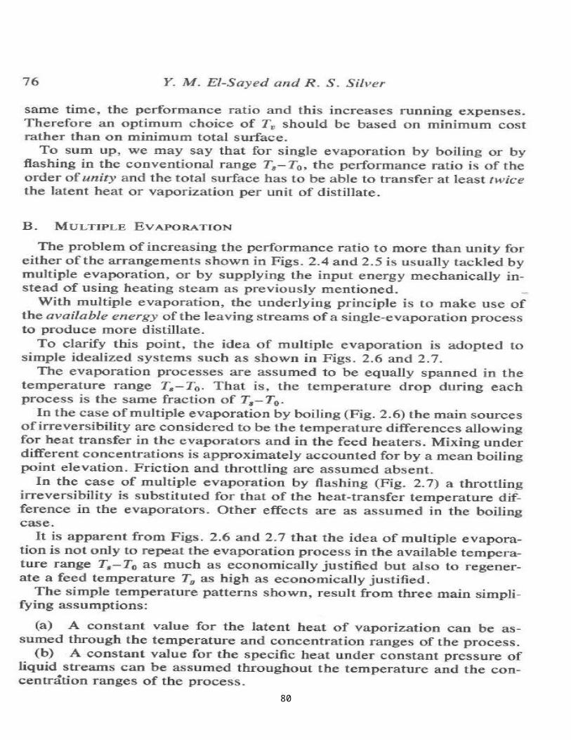
1. INTRODUCTION

1.1 IMPORTANCE OF DESALINATION

3

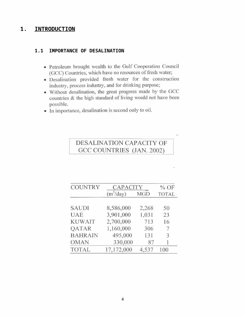
4

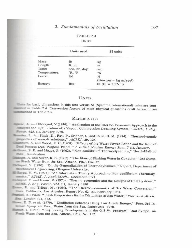
DESALINATION PLANTS CAPACITIES BY PROCESS (2011)

(Source: MENA Regional Water Outlook, Fichtner 2011)

5

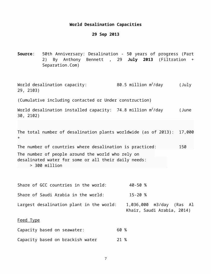
World Desalination Capacities

29 Sep 2013

Source: 50th Anniversary: Desalination - 50 years of progress (Part 2) By Anthony Bennett , 29 July 2013 (Filtration + Separation.Com)

World desalination capacity: 80.5 million m3/day (July 29, 2103)

(Cumulative including contacted or Under construction)

World desalination installed capacity: 74.8 million m3/day (June 30, 2102)

The total number of desalination plants worldwide (as of 2013): 17,000 +

The number of countries where desalination is practiced: 150

The number of people around the world who rely on desalinated water for some or all their daily needs: > 300 million

Share of GCC countries in the world: 40-50 %

Share of Saudi Arabia in the world: 15-20 %

Largest desalination plant in the world: 1,036,000 m3/day (Ras Al Khair, Saudi Arabia, 2014)

Feed Type

Capacity based on seawater: 60 %

Capacity based on brackish water 21 %

Capacity based on treating waste water 6 %

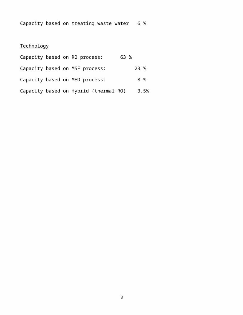
Technology

Capacity based on RO process: 63 %

Capacity based on MSF process: 23 %

Capacity based on MED process: 8 %

6

Capacity based on Hybrid (thermal+RO) 3.5%

7

1.2 WORLD WATER

http://www.waterworld.com/articles/2013/10/global-desalination-capacity-tops-80-million-cubic-meters-per-day.html

Global desalination capacity growing substantially, finds study

TOPSFIELD, MA, and LONDON, Oct. 14, 2013 -- According to new data from the International Desalination Association, the amount of new desalination capacity expected to come online during 2013 is 50 percent more than last year's total. Desalination plants with a total capacity of 6 million cubic meters per day (m3/d) are expected to come online during 2013, compared with 4 million m3/d in 2012.

Seawater desalination continues to represent the largest percentage of online global capacity at 59%, followed by brackish water at 22%, river water at 9%, and wastewater and pure water at 5% each.

In 2013: The top 10 seawater desalination countries by online capacity are:

CountryCommissioned seawater desalination

capacity m3/d

Saudi Arabia 9,170,391

UAE 8,381,299

Spain 3,781,314

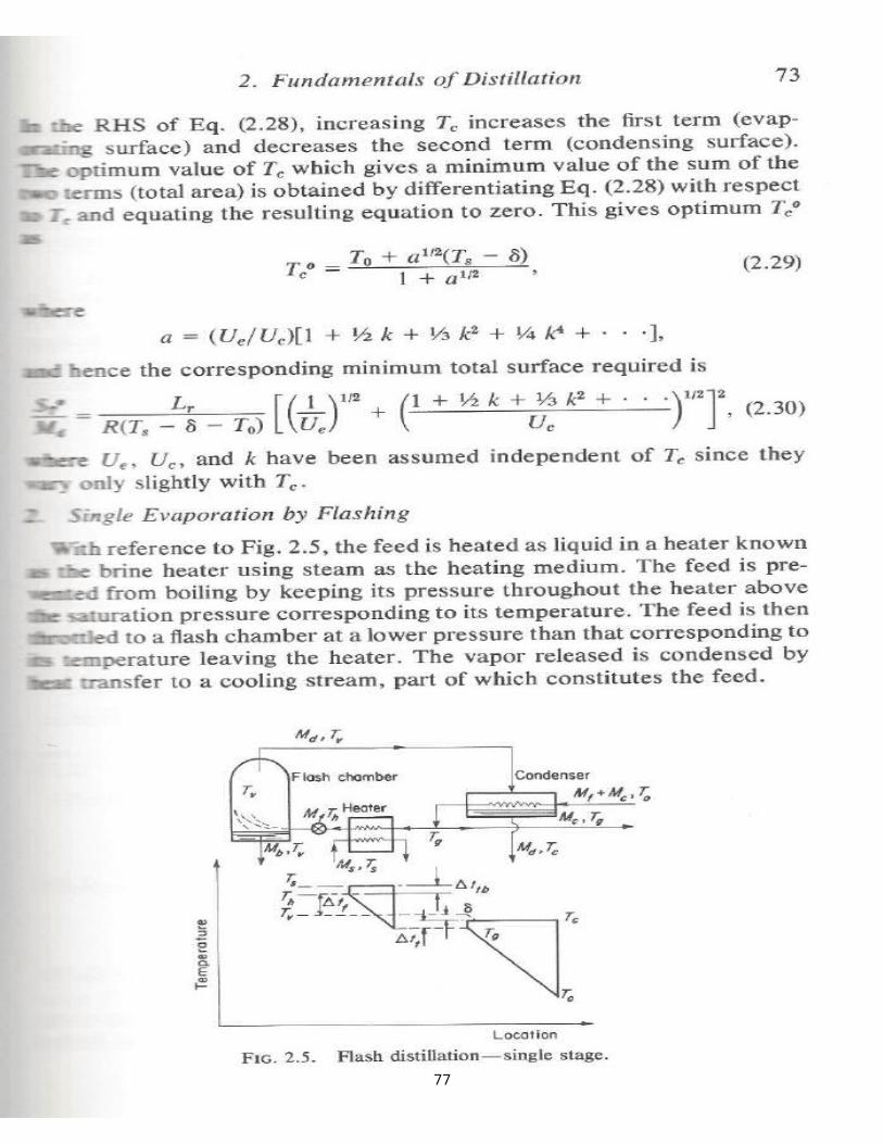
Kuwait 2,586,761

Algeria 2,364,055

Australia 1,823,154

Qatar 1,780,708

Palestinian Occupied Territories 1,532,723

China 1,494,198

Libya 1,048,424

The markets which are expected to see the fastest growth in desalination over the next five years are South Africa, Jordan, Mexico, Libya, Chile, India, and China, all of which are expected to more than double their desalination capacity.

8

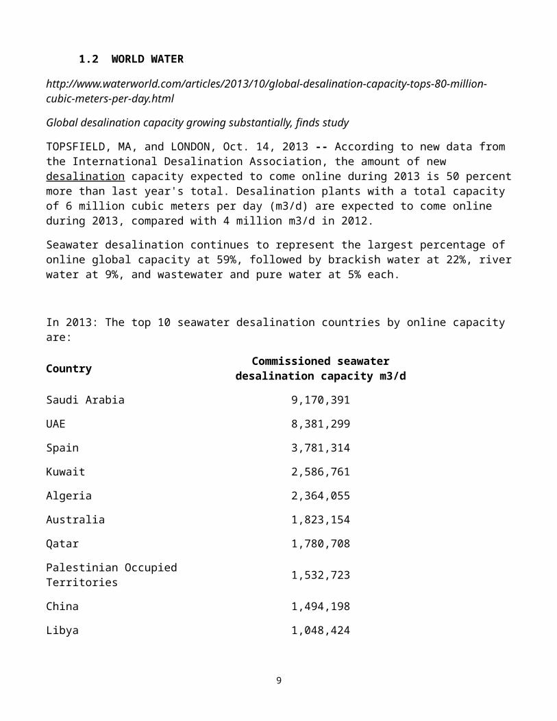
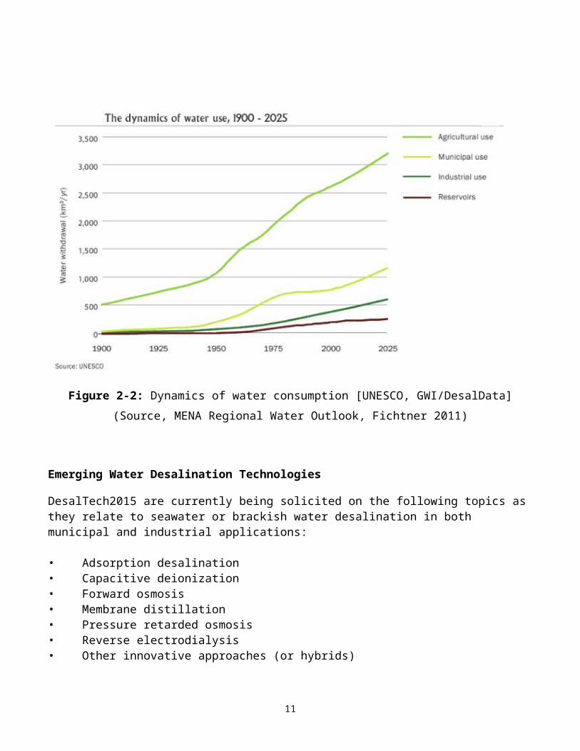
Figure 2-2: Dynamics of water consumption [UNESCO, GWI/DesalData]

(Source, MENA Regional Water Outlook, Fichtner 2011)

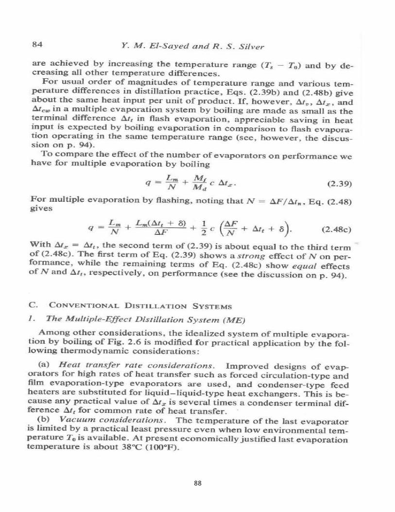
Emerging Water Desalination Technologies

DesalTech2015 are currently being solicited on the following topics as they relate to seawater or brackish water desalination in both municipal and industrial applications:    •    Adsorption desalination•    Capacitive deionization•    Forward osmosis•    Membrane distillation•    Pressure retarded osmosis•    Reverse electrodialysis•    Other innovative approaches (or hybrids)

9

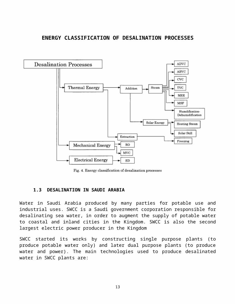
ENERGY CLASSIFICATION OF DESALINATION PROCESSES

1.3 DESALINATION IN SAUDI ARABIA

Water in Saudi Arabia produced by many parties for potable use and industrial uses. SWCC is a Saudi government corporation responsible for desalinating sea water, in order to augment the supply of potable water to coastal and inland cities in the Kingdom. SWCC is also the second largest electric power producer in the Kingdom

SWCC started its works by constructing single purpose plants (to produce potable water only) and later dual purpose plants (to produce water and power). The main technologies used to produce desalinated water in SWCC plants are:

Multistage Flash (MSF )

Reverse Osmosis (RO)

10

VISSION :

“Excellence in development research of saline water desalination technologies”

MISSION :

“To develop saline water desalination technologies by conducting innovative research studies towards making the Institute worldwide recognized scientific reference”

Major SWCC Desalination Plants in Operation (m3/day) in Saudi Arabia:

Western Coast

1

JEDDAH MSF = 304,000

RO = 100,000

2AL-SHOAIBAH MSF = 583,000

3

YANBU MSF = 215,000

RO = 107,000

4AL-SHUQAIQ MSF = 83,000

5HAQL RO = 4,000

6DUBA RO = 4,000

7AL-WAJH MSF = 1,500

8UMMLUJ RO = 4,000

9RABIGH MSF = 2,000

10AL-AZIZIYAH RH = 4,000

11AL-BIRK RO = 2,000

12FARASAN MSF = 1,500

Eastern Coast

1AL-KHOBAR MSF = 433,000

2

AL-JUBAIL MSF = 934,000

RO = 78,000

3AL-KHAFJI MSF = 20,000

11

LOCATIONS OF MSF DESALINATION PLANTS IN SAUDI ARABIA

The Institute’s Main Objectives :

1. Transfer and develop saline water desalination technologies.2. Distinguished research in saline water desalination.3. Cost reduction of desalinated water production.4. Provide scientific solutions for the technical problems in desalination plants and water transmission systems.5. Monitoring the product water quality and maintaining protected environment according to national and international guidelines.6. Marketing the technical services locally and worldwide, and develop commercial based work procedures. 7. Develop qualified Saudi researchers specialized in the saline water desalination. 8. Promoting scientific and technical capabilities through cooperation with national and international research institutes.

12

The Institute’s Departments :

1. Technical (Corrosion and Metallurgy, Chemistry, Marine Biology and Environment)2. Engineering (Thermal, Seawater Reverse Osmosis)3. Support (Planning, administration, pilot plants)

13

HISTORY OF DESALINATION IN SAUDI ARABIA

1928 G - 1348 H : Establishment of the First Two Sea Water condensers at Jeddah became Known as "AL-KANDASA ."

1965 G - 1385 H : An Office has been opened at The Ministry of Agriculture & Water for feasibility study and the preparatory steps

for Desalination Plants construction .

1969 G - 1389 H : Opening “PHASE I” of Al-Wajh and Duba Plants .

1970 G - 1390 H : Opening of Jeddah Plant “ PHASE I . “

1972 G - 1392 H : A Saline Water Conversion Agency has been established at the Ministry of Agriculture & Water .

1973 G - 1393 H : Opening Al-Khobar ( Phase I ) Plant .

1974 G - 1394 H : Issue of Royal Decree No. M/49 Establishing “ SALINE WATER CONVERSION CORPORATION “ as an

Independent Body .

1974 G - 1394 H : Opening of Al-Khafji “PHASE I” Plant .

1975 G - 1395 H : Opening Ummluj “PHASE I” Plant .

1978 G - 1398 H : Opening Jeddah “PHASE II” Plant .

1979 G - 1399 H : Opening Four Plants at Al-Wajh, Duba “PHASE II”, Farasan “PHASE I” and Jeddah “PHASE III . ”

1980 G - 1400 H : Opening of Haql “ PHASE I” Plant .

1981 G - 1401 H : Madinah / Yanbu “PHASE I” Plant .

1982 G - 1402 H : Opening Three Plants at Al-Jubail “PHASE I, Rabigh “PHASE I”, Jeddah “PHASE IV” and The Training Center at

Jubail, which started its First Session .

1983 G - 1403 H : Opening Al-Birk “Phase I” Plant, Al-Jubail and Al-Khobar “PHASE II’ Plants .

1986 G - 1406 H : Opening Al-Wajh “First Extension” Plant, Al-Khafji and Ummluj “PHASE II” Plants .

1987 G - 1407 H : Opening of Al-Aziziyah “PHASE I” Plant and The Research & Development and Training Center (RDTC) at Al-

Jubail plant site .

1989 G - 1409 H :

14

Opening Five Plants at Duba “PHASE III”, Al-Wajh ‘Second Extension’, Jeddah R.O. “PHASE I”, Al-Shoaibah ‘Phase I “ and Al-Shuqaiq “PHASE I .“

1990 G - 1410 H : Opening of Haql “PHASE II” Plant and Farasan “First Extension” Plant .

1994 G - 1414 H : Opening of Jeddah R.O. “PHASE II” Plant .

1999 G - 1420 H : Opening of Yanbu MSF and R.O. “PHASE II” Plants .

2001 G - 1422 H : Opening of Al-Khobar MSF. “PHASE III” & Al-Jubail R.O Plant

2002 G - 1423 H : Opening of Al-Shoaibah “PHASE II .”

2004 G - 1425 H : Operation of Khobar, Alhasa & Abgaig Pipelines, the issue of SWCC Governor Decree No. (33528) dated 5/7/1425 H to build a strategic team to study the required procedures for SWCC privatization and restructuring.

2005 G - 1426 H : Shoaiba Plant Phase- III Project for water desalination and power production has been awarded. In addition Al-Wajh phase III, Umluj phase-III, Rabigh phase II, Laith and Qunfudah phase-I, and Farasan phase-II projects have also been awarded. Consulting companies have been assigned to study the aspects of restructure and privatization programme of SWCC.

2006 G - 1427 H : Procurement & construction contracts of Shoaiba (phase-III) Transmission System were signed and sites were handed over. Procurement & Construction contracts of New Satellite Plants (Al -Wajh, Rabigh, Laith, Qunfudah, Farasan, Umluj) and their Pipelines were signed and sites were handed over, assigned to study the aspects of restructure and privatization programme of SWCC

15

YearAnnual Water ProductionAnnual Electricity Production

(Million m3) (Million MegaWatt/Hour)

1980 7.650.22

1981 60.95 1.74

1982 111.65 2.87

1983 199.49 5.32

1984 321.43 9.88

1985 390.08 12.59

1986 449.98 14.01

1987 508.42 16.07

1988 521.55 16.08

1989 609.29 17.81

1990 653.70 20.76

1991 660.91 19.59

1992 683.11 21.12

1993 692.36 21.59

1994 715.03 21.67

1995 706.17 22.78

1996 728.13 21.00

1997 727.26 21.06

1998 740.78 21.83

1999 775.00 22.28

2000 797.38 22.04

2001 857.41 23.2

2002 863.20 18.68

2003 982.89 24.20

2004 1064.90 21.81

20051025.0521.06

20061034.1322.62

20071092.9429.72

20081096,7029.00

20091014.2126.52

2010883.824.7

16

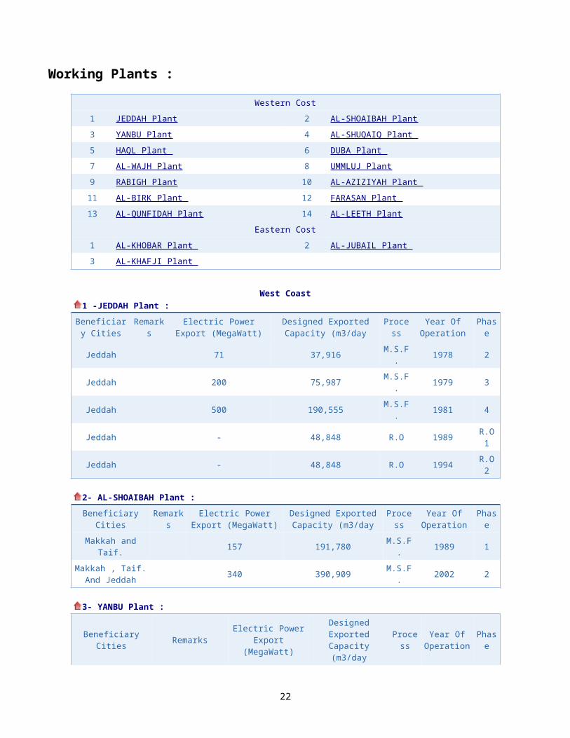
Working Plants :

Western Cost

1 JEDDAH Plant 2 AL-SHOAIBAH Plant

3 YANBU Plant 4 AL-SHUQAIQ Plant

5 HAQL Plant 6 DUBA Plant

7 AL-WAJH Plant 8 UMMLUJ Plant

9 RABIGH Plant 10 AL-AZIZIYAH Plant

11 AL-BIRK Plant 12 FARASAN Plant

13 AL-QUNFIDAH Plant 14 AL-LEETH Plant

Eastern Cost

1 AL-KHOBAR Plant 2 AL-JUBAIL Plant

3 AL-KHAFJI Plant

West Coast1 -JEDDAH Plant :

Phase

Year Of Operation

Process

Designed Exported Capacity (m3/day

Electric Power Export (MegaWatt)

Remarks

Beneficiary Cities

21978M.S.F.37,91671Jeddah

31979M.S.F.75,987200Jeddah

41981M.S.F.190,555500Jeddah

R.O 1

1989R.O48,848-Jeddah

R.O 2

1994R.O48,848-Jeddah

2- AL-SHOAIBAH Plant :

Phase

Year Of Operation

Process

Designed Exported Capacity (m3/day

Electric Power Export (MegaWatt)

Remarks

Beneficiary Cities

11989M.S.F.191,780157Makkah and Taif.

22002M.S.F.390,909340Makkah , Taif.

And Jeddah

3- YANBU Plant :

Phase

Year Of Operation

Process

Designed Exported

Capacity (m3/day

Electric Power Export

(MegaWatt)RemarksBeneficiary Cities

11981M.S.F.94,625250Madina and

Yanbu.

21999M.S.F.120,09635Madina, Yanbu and adjacent

cities.

R.O1999R.O.106,904-The largest R.O.

plant in the world.

Madina, Yanbu and adjacent

cities.

17

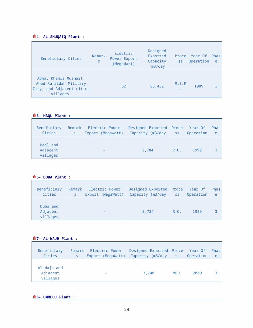
4- AL-SHUQAIQ Plant :

Phase

Year Of Operation

Process

Designed Exported Capacity (m3/day

Electric Power Export

(MegaWatt)

Remarks

Beneficiary Cities

11989M.S.F.83,43262Abha, Khamis Mushait, Ahad Rufaidah Military City, and

Adjacent cities villages.

5- HAQL Plant :

Phase

Year Of Operation

Process

Designed Exported Capacity (m3/day

Electric Power Export (MegaWatt)

Remarks

Beneficiary Cities

21990R.O.3,784-Haql and

Adjacent villages

6- DUBA Plant :

Phase

Year Of Operation

Process

Designed Exported Capacity (m3/day

Electric Power Export (MegaWatt)

Remarks

Beneficiary Cities

31989R.O.3,784-Duba and

Adjacent villages

7- AL-WAJH Plant :

Phase

Year Of Operation

Process

Designed Exported Capacity (m3/day

Electric Power Export (MegaWatt)

Remarks

Beneficiary Cities

32009MED.7,740-. Al-Wajh and

Adjacent villages

8- UMMLUJ Plant :

Phase

Year Of Operation

Process

Designed Exported Capacity (m3/day

Electric Power Export (MegaWatt)

Remarks

Beneficiary Cities

R.O1986R.O.3,784-Ummluj

32009MED7,740-Ummluj and Adjacent villages

18

9- RABIGH Plant :

Phase

Year Of Operation

Process

Designed Exported Capacity (m3/day

Electric Power Export (MegaWatt)

Remarks

Beneficiary Cities

22009MED15,480-Rabigh - Mastorah - Thoal

10- AL-AZIZIYAH Plant :

Phase

Year Of Operation

Process

Designed Exported Capacity (m3/day

Electric Power Export (MegaWatt)

Remarks

Beneficiary Cities

11987R.H.3,870-Al-Aziziyah

Island.

11- AL-BIRK Plant :

Phase

Year Of Operation

Process

Designed Exported Capacity (m3/day

Electric Power Export (MegaWatt)

Remarks

Beneficiary Cities

11983R.O1,952-Al-Birk and

Adjacent villages.

12- FARASAN Plant :

22009MED.7,740-Farasan Island.

Transferred 11990M.S.F.1,075-Transferred from AL-Khafji. Farasan Island.

13- AL-QUNFIDAH Plant :

Phase

Year Of Operation

Process

Designed Exported Capacity (m3/day

Electric Power Export (MegaWatt)

Remarks

Beneficiary Cities

12008MED7,740-Al-Qunfidhah, Al-

qooz and hali

14- AL-LEETH Plant :

Phase

Year Of Operation

Process

Designed Exported Capacity (m3/day

Electric Power Export (MegaWatt)

Remarks

Beneficiary Cities

19

12009MED7,740-Al-Leeth

East Coast

1- AL-KHOBAR Plant :

Phase

Year Of Operation

Process

Designed Exported Capacity (m3/day

Electric Power Export

(MegaWatt)

Remarks

Beneficiary Cities

21982M.S.F.191,780500Khobar, Dammam, Dhahran Airport, Qatif, Saihat, Safwa,

and Ras Tannourah.

32002M.S.F.240,800311

Khobar, Dammam, Dhahran Airport, Qatif, Saihat, Safwa, Ras Tannourah, Hofuf and

Bgaig

2- AL-JUBAIL Plant :

Phase

Year Of Operation

Process

Designed Exported Capacity (m3/day

Electric Power Export

(MegaWatt)

Remarks

Beneficiary Cities

11982M.S.F.118,447238Riyadh, Jubail, Marine Base,

and Sadaf.

21983M.S.F.815,185762Riyadh, Jubail, Marine Base,

and Sadaf.

RO2002RO78,182-Riyadh,Sudair,Washim,Qassi

m

3- AL-KHAFJI Plant :

Phase

Year Of Operation

Process

Designed Exported Capacity (m3/day

Electric Power Export (MegaWatt)

Remarks

Beneficiary Cities

21986M.S.F.19,682-Al-Khafji

20

THE ADDITIONNAL OF WATER & POWER EXPORT CAPACITY FOR FUTURE DEMAND OF (PRIVATE SECTOR ) DESALINATION PLANTS

PROJECT NAME Water Total Exportation ( M3/day )Total Electricity Exportation (MWH )

Shuqaiq Phase -II212,000 850

Marafig Company Project500,000 0

Al Shoaibah Phase –III880,000 900

Al Shoaibah R.O150,0000

Plants Under Construction : Total Electric Power

Export ( MW )Total Water Export.

( m3/day )Project Name

2,4001,025,000RAS ALKHAIR

2,500550,000Yanbu 3

4,9001,575,000TOTAL ADDITIONNAL EXPORT CAPACITY FOR FUTURE DEMAND

21

2. QUALITY OF WATER AND APPLICATIONS:

Total dissolved solids (TDS) is the term used to describe the inorganic salts and small amounts of organic matter present in solution in water. The principal constituents are usually calcium, magnesium, sodium, and potassium cations and carbonate, hydrogen carbonate, chloride, sulfate, and nitrate anions.

The presence of dissolved solids in water may affect its taste. The palatability of drinking water has been rated by panels of tasters in relation to its TDS level as follows: excellent, less than 300 mg/litre; good, between 300 and 600 mg/litre; fair, between 600 and 900 mg/litre; poor, between 900 and 1200 mg/litre; and unacceptable, greater than 1200 mg/litre . Water with extremely low concentrations of TDS may also be unacceptable because of its flat, insipid taste.

No recent data on health effects associated with the ingestion of TDS in drinking-water appear to exist; however, associations between various health effects and hardness, rather than TDS content, have been investigated in many studies. In early studies, inverse relationships were reported between TDS concentrations in drinking water and the incidence of cancer, coronary heart disease, arteriosclerotic heart disease, and cardiovascular disease. Total mortality rates were reported to be inversely correlated with TDS levels in drinking-water.

It was reported in a summary of a study in Australia that mortality from all categories of ischemic heart disease and acute myocardial infarction was increased in a community with high levels of soluble solids, calcium, magnesium, sulfate, chloride, fluoride, alkalinity, total hardness, and pH when compared with one in which levels were lower. No attempts were made to relate mortality from cardiovascular disease to other potential confounding factors.

Certain components of TDS, such as chlorides, sulfates, magnesium, calcium, and carbonates, affect corrosion or encrustation in water-distribution systems. High TDS levels (>500 mg/litre) result in excessive scaling in water pipes, water heaters, boilers, and household appliances such as kettles and steam irons. Such scaling can shorten the service life of these appliances.

Water containing TDS concentrations below 1000 mg/litre is usually acceptable to consumers, although acceptability may vary according to circumstances. However, the presence of high levels of TDS in water may be objectionable to consumers owing to the resulting taste and to excessive scaling in water pipes, heaters, boilers, and household appliances. Water with extremely low concentrations of TDS may also be unacceptable to consumers because of its flat, insipid taste; it is also often corrosive to water-supply systems. In areas where the TDS content of the water supply is very high, the individual constituents should be identified and the local public health authorities consulted. No health-based guideline value is proposed for TDS. However, drinking-water guidelines are available for some of its constituents, including boron, fluoride, and nitrate.

Source: WHO Guidelines for Drinking-water Quality

TDS levels in drinking water should preferably be monitored especially when a reversed osmosis is used for raw water purification. A minimum TDS of 100mg/liter (100 ppm, parts per million) should be set. A maximum of 500mg/Liter (500 ppm) is the upper limit. Water with a TDS above 500 ppm will have a salty taste. Studies by the World Health Organization also showed that water dranked by rats, dogs and cats with solids below 100 ppm had bad effects on the animal's stomach.

Source: www.TDS in drinking water.

Most people think of TDS as being an aesthetic factor. In a study by the World Health Organization, a panel of tasters came to the following conclusions about the preferable level of TDS in Water

water: Level of TDS (milligrams per litre) Rating Less than 300 Excellent

22

300 - 600 Good 600 - 900 Fair 900 - 1,200 Poor Above 1,200 Unacceptable

Taste of Water with Different TDS Concentrations; www.who.int/water_sanitation_health/dwq/chemicals/tds.pdf

However, a very low concentration of TDS has been found to give water a flat taste, which is undesirable to many people.

Increased concentrations of dissolved solids can also have technical effects. Dissolved solids can produce hard water, which leaves deposits and films on fixtures, and on the insides of hot water pipes and boilers. Soaps and detergents do not produce as much lather with hard water as with soft water. As well, high amounts of dissolved solids can stain household fixtures, corrode pipes, and have a metallic taste. Hard water causes water filters to wear out sooner, because of the amount of minerals in the water. The picture below was taken near the Mammoth Hot Springs, in Yellowstone National Park, and shows the effect that water with high concentrations of minerals can have on the landscape. The same minerals that are deposited on these rocks can cause problems when they build up in pipes and fixtures.

What is pH of Water?

The pH value of a water source is a measure of its acidity or alkalinity. The pH level is a measurement of the activity of the hydrogen atom, because the hydrogen activity is a good representation of the acidity or alkalinity of the water. The pH scale, as shown below, ranges from 0 to 14, with 7.0 being neutral. Water with a low pH is said to be acidic, and water with a high pH is basic, or alkaline. Pure water would have a pH of 7.0, but water sources and precipitation tends to be slightly acidic, due to contaminants that are in the water.

23

Like TDS, pH is given an aesthetic objective in Canada. The Canadian Guidelines for Drinking Water Quality suggest that the pH of drinking water should be between 6.5 and 8.5. The Saskatchewan guidelines recommend that the pH of drinking water be between 6.5 and 9.0. In the United States, pH is, like TDS, a secondary standard; the Secondary Maximum Contaminant Level for pH is between 6.5 and 8.5. According to the EPA, the noticeable effects of a pH that is less than 6.5 include a bitter, metallic taste and corrosion. The noticeable effects of a pH above 8.5 include a slippery feeling, soda-like taste and deposits.

There are several methods that can increase the pH of water, before disinfection. The pH is commonly increased using sodium carbonate and sodium hydroxide, but a better way of dealing with low pH is to use calcium and magnesium carbonate, which not only will increase pH levels, but will also make the water less corrosive and both calcium and magnesium are of health benefits as opposed to sodium.

Source: www.safewater.org

24

3. CHEMISTRY AND PROPERTIES OF SALINE WATER

3.1 Basic Definitions

25

DIFFERENT TYPES OF WATER CONCENTRATION UNITS

Molarity (M) = Moles solute/L.Soln.

Molality (m) = Moles Solute/1 kg H2O

Weight percent (Wt. %) = gm of Solute/100 gm soln.

RELATIONS AMONG MOLARITY (M); MOLALITY (m) AND WT. % CONCENTRATIONS

Given (m), Change to (M) :

Given (M), Change to (m) :

Given (Wt.%), Change to (M) :

Given (Wt.%), Change to (m) :

Where:

MW = MOL. Weight of Solute

= Density of Solution

26

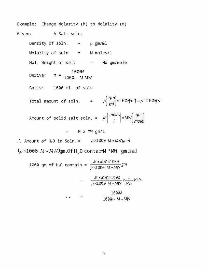
Example: Change Molarity (M) to Molality (m)

Given: A Salt soln.

Density of soln. = gm/ml

Molarity of soln = M moles/l

Mol. Weight of salt = MW gm/mole

Derive: m =

Basis: 1000 ml. of soln.

Total amount of soln. =

Amount of solid salt soln. =

= M x MW gm/l

Amount of H2O in Soln. =

1000 gm of H2O contain =

=

=

27

Ionic strength(From Wikipedia )

The ionic strength of a solution is a measure of the concentration of ions in that solution. Ionic compounds, when dissolved in water, dissociate into ions. The total electrolyte concentration in solution will affect important properties such as the dissociation or the solubility of different salts. One of the main characteristics of a solution with dissolved ions is the ionic strength.

QUANTIFYING IONIC STRENGTH

The ionic strength, I, of a solution is a function of the concentration of all ions present in that solution.

where ci is the molar concentration of ion i(mol·dm-3), zi is the charge number of that ion, and the sum is taken over all ions in the solution. For a 1:1 electrolyte such as sodium chloride, the ionic strength is equal to the concentration, but for MgSO4 the ionic strength is four times higher. Generally multivalent ions contribute strongly to the ionic strength.

Note:

Because in non-ideal solutions volumes are no longer strictly additive it is often preferable to work with molality (mol/kg{H2O}) rather than molarity (mol/L). In that case, ionic strength is defined as:

i = individual element z = charge of element

IMPORTANCE

The ionic strength plays a central role in the Debye–Hückel theory that describes the strong deviations from ideality typically encountered in ionic solutions.

Media of high ionic strength are used in stability constant determination in order to minimize changes, during a titration, in the activity quotient of solutes at lower concentrations. Natural waters such as seawater have a non-zero ionic strength due to the presence of dissolved salts which significantly affects their properties.

28

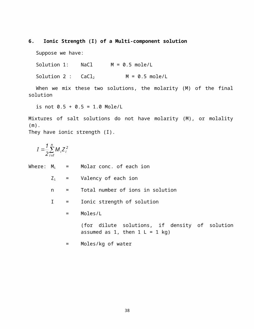
6. Ionic Strength (I) of a Multi-component solution

Suppose we have:

Solution 1: NaCl M = 0.5 mole/L

Solution 2 : CaCl2 M = 0.5 mole/L

When we mix these two solutions, the molarity (M) of the final solution

is not 0.5 + 0.5 = 1.0 Mole/L

Mixtures of salt solutions do not have molarity (M), or molality (m).They have ionic strength (I).

Where: Mi = Molar conc. of each ion

Zi = Valency of each ion

n = Total number of ions in solution

I = Ionic strength of solution

= Moles/L

(for dilute solutions, if density of solution assumed as 1, then 1 L = 1 kg)

= Moles/kg of water

29

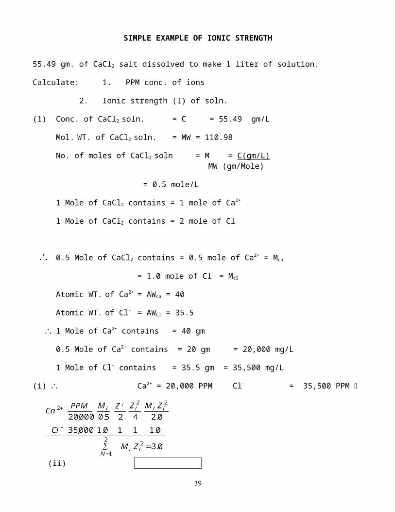
SIMPLE EXAMPLE OF IONIC STRENGTH

55.49 gm. of CaCl2 salt dissolved to make 1 liter of solution.

Calculate: 1. PPM conc. of ions

2. Ionic strength (I) of soln.

(1) Conc. of CaCl2 soln. = C = 55.49 gm/L

Mol. WT. of CaCl2 soln. = MW = 110.98

No. of moles of CaCl2 soln = M = C(gm/L) MW (gm/Mole)

= 0.5 mole/L

1 Mole of CaCl2 contains = 1 mole of Ca2+

1 Mole of CaCl2 contains = 2 mole of Cl-

0.5 Mole of CaCl2 contains = 0.5 mole of Ca2+ = Mca

= 1.0 mole of Cl- = Mcl

Atomic WT. of Ca2+ = AWca = 40

Atomic WT. of Cl- = AWcl = 35.5

1 Mole of Ca2+ contains = 40 gm

0.5 Mole of Ca2+ contains = 20 gm = 20,000 mg/L

1 Mole of Cl- contains = 35.5 gm = 35,500 mg/L

(i) Ca2+ = 20,000 PPM Cl- = 35,500 PPM

(ii)

30

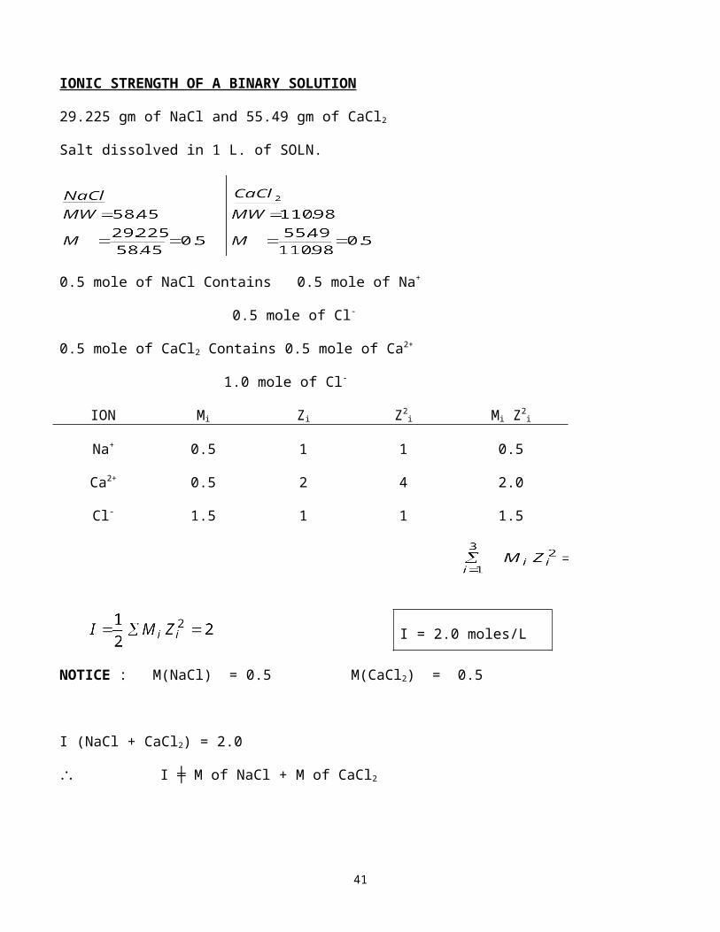
IONIC STRENGTH OF A BINARY SOLUTION

29.225 gm of NaCl and 55.49 gm of CaCl2

Salt dissolved in 1 L. of SOLN.

0.5 mole of NaCl Contains 0.5 mole of Na+

0.5 mole of Cl-

0.5 mole of CaCl2 Contains 0.5 mole of Ca2+

1.0 mole of Cl-

ION Mi Zi Z2i Mi Z2

i

Na+ 0.5 1 1 0.5

Ca2+ 0.5 2 4 2.0

Cl- 1.5 1 1 1.5

I = 2.0 moles/L

NOTICE : M(NaCl) = 0.5 M(CaCl2) = 0.5

I (NaCl + CaCl2) = 2.0

I ╪ M of NaCl + M of CaCl2

31

7. SALINITY: Total dissolved solids (TDS) in gm present in 1 kg. of seawater, after all HCO -3

(Bicarbonate) and CO2-3 (Carbonate) have been converted to equivalent oxide, and Br- (Bromide) and I -

(Iodine), and all organic matter oxidized.

Mg/kg Eq.wt.

Seawater TDS 34,481 -

HCO-3 140 61

CO2-3 0 30

Br- 65 79.91

TDS without CO2-3, HCO-

3, Br- = 34,481 – (140 + 65)

= 34,276

EQ. Wt. of Cl- = 35.45,

EQ. Wt. of O- (oxide) = 8

EQ. Wt. of Br- = 79.91

Salinity = 34,276

= 34,276+ 18 + 29

= 34,323 mg/kg seawater

= 0.5% lower than TDS.

32

CLASSIFICATION OF SALINE WATER

Water salinity

Fresh water Brackish water Saline water Brine

< 0.05 % 0.05 – 3 % 3 – 5 % > 5 %

< 0.5 ppt 0.5 – 30 ppt 30 – 50 ppt > 50 ppt

Mangrove swamps are coastal wetlands found in tropical and subtropical regions. They are

characterized by halophytic (salt loving) trees, shrubs and other plants growing in brackish to

saline tidal waters. These wetlands are often found in estuaries, where fresh water meets salt

water.

33

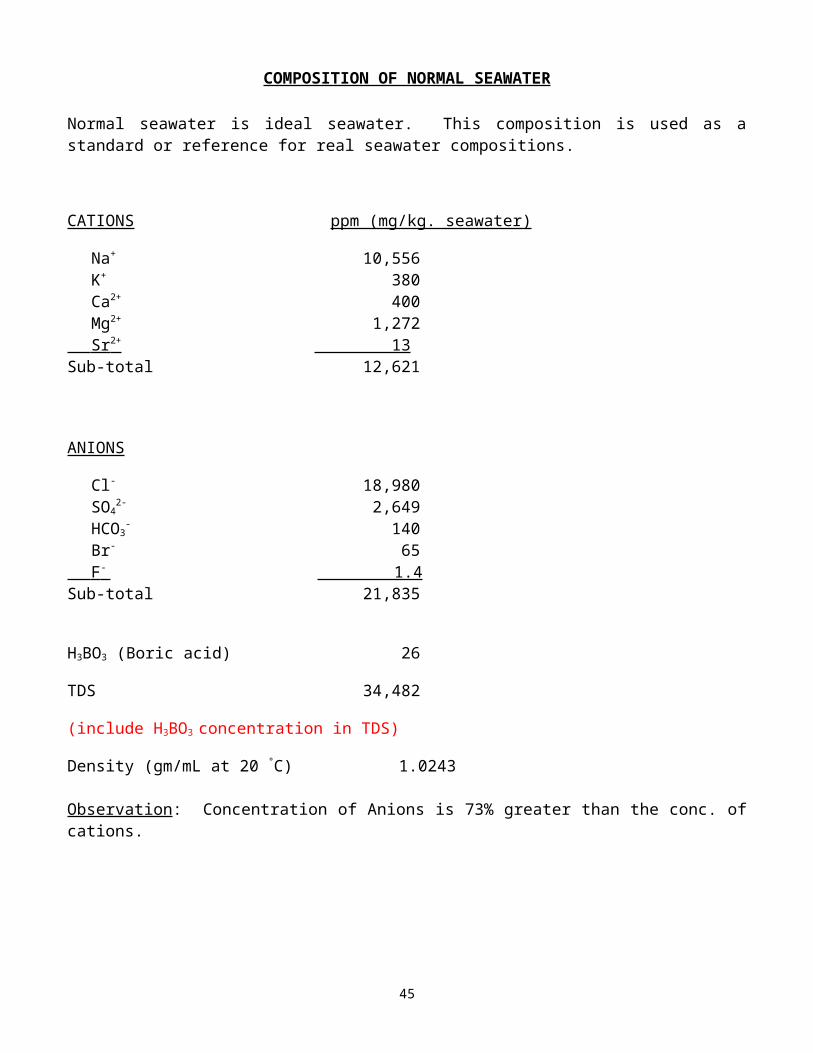
COMPOSITION OF NORMAL SEAWATER

Normal seawater is ideal seawater. This composition is used as a standard or reference for real seawater compositions.

CATIONS ppm (mg/kg. seawater)

Na+ 10,556K+ 380Ca2+ 400Mg2+ 1,272

Sr 2+ 13 Sub-total 12,621

ANIONS

Cl- 18,980SO4

2- 2,649HCO3

- 140Br- 65

F - 1.4 Sub-total 21,835

H3BO3 (Boric acid) 26

TDS 34,482

(include H3BO3 concentration in TDS)

Density (gm/mL at 20 °C) 1.0243

Observation: Concentration of Anions is 73% greater than the conc. of cations.

34

MOLECULAR COMPOSITION OF NORMAL SEAWATER

CATIONS ppm (mg/kg.) %

NaCl 23,476 68.1

MgCl2 4,981 14.4

Na2SO4 3,917 11.4

CaCl2 1,102 3.2

KCl 664 1.9

NaHCO3 192 0.5

KBr 96 0.3

H3BO3 26 0.1

SrCl2 24 0.1

NaF 3 0.0 TOTAL 34,481 100.0

OBSERVATIONS:

(1) Major constituent of seawater is NaCl salt (68%).

(2) 3 out of 10 salts (NaCl, MgCl2, Na2SO4) account for 94% of seawater TDS.

35

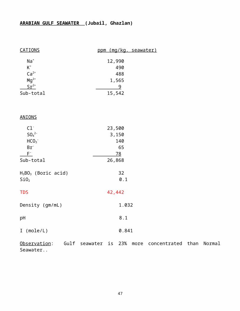
ARABIAN GULF SEAWATER (Jubail, Ghazlan)

CATIONS ppm (mg/kg. seawater)

Na+ 12,990K+ 490Ca2+ 488Mg2+ 1,565

Sr 2+ 9 Sub-total 15,542

ANIONS

Cl- 23,500SO4

2- 3,150HCO3

- 140Br- 65

F - 78 Sub-total 26,868

H3BO3 (Boric acid) 32SiO2 0.1

TDS 42,442

Density (gm/mL) 1.032

pH 8.1

I (mole/L) 0.841

Observation: Gulf seawater is 23% more concentrated than Normal Seawater..

36

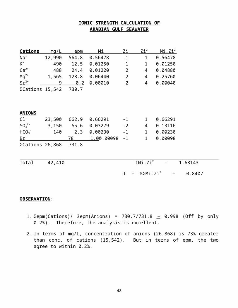
IONIC STRENGTH CALCULATION OFARABIAN GULF SEAWATER

Cations mg/L epm Mi Zi Zi 2 Mi.Zi 2 Na+ 12,990 564.8 0.56478 1 1 0.56478K+ 490 12.5 0.01250 1 1 0.01250Ca2+ 488 24.4 0.01220 2 4 0.04880Mg2+ 1,565 128.8 0.06440 2 4 0.25760Sr 2+ 9 0.2 0.00010 2 4 0.00040ΣCations 15,542 730.7

ANIONSCl- 23,500 662.9 0.66291 -1 1 0.66291SO4

2- 3,150 65.6 0.03279 -2 4 0.13116HCO3

- 140 2.3 0.00230 -1 1 0.00230Br - 78 1.0 0.00098 -1 1 0.00098ΣCations 26,868 731.8

Total 42,410 ΣMi.Zi2 = 1.68143

I = ½ΣMi.Zi2 = 0.8407

OBSERVATION:

1. Σepm(Cations)/ Σepm(Anions) = 730.7/731.8 0.998 (Off by only 0.2%). Therefore, the analysis is excellent.

2. In terms of mg/L, concentration of anions (26,868) is 73% greater than conc. of cations (15,542). But in terms of epm, the two agree to within 0.2%.

37

CRITERION FOR ACCEPTING OR REJECTING WATER ANALYSIS

1. If 0.97 Σepm(Cations)/ Σepm(Anions) 1.03,i.e. if the ratio is greater than or equal to 0.97, or equal to 1.03, the analysis is good.

In such a case, the sum of epm cations and sum of epm anions agree to within 3%

2. If the sum of epm cations and sum of epm anions do not agree to within 3% then the analysis is unbalanced and unacceptable.

3. If however, the unbalanced analysis just has to be used, then:

3.1 If Σepm(Cations)/ Σepm(Anions) Σepm(Anions) i.e. some Cations are missing, the difference is made up by adding Na+ ions, until the two are exactly equal;

3.2 If Σepm(Anions) Σepm(Cations)i.e. some Anions are missing, the difference is made up by adding Cl- ions, until the two are exactly equal;

38

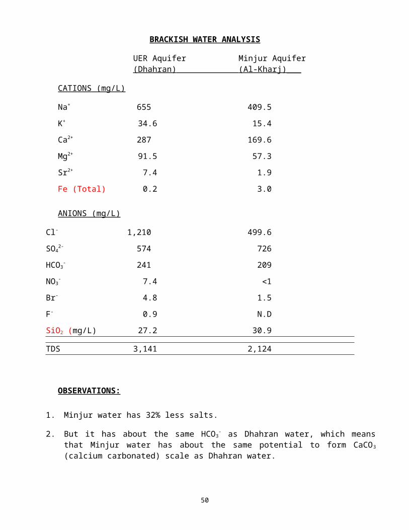
BRACKISH WATER ANALYSIS

UER Aquifer Minjur Aquifer(Dhahran) (Al-Kharj)___

CATIONS (mg/L)

Na+ 655 409.5

K+ 34.6 15.4

Ca2+ 287 169.6

Mg2+ 91.5 57.3

Sr2+ 7.4 1.9

Fe (Total) 0.2 3.0

ANIONS (mg/L)

Cl- 1,210 499.6

SO42- 574 726

HCO3- 241 209

NO3- 7.4 1

Br- 4.8 1.5

F- 0.9 N.D

SiO2 (mg/L) 27.2 30.9

TDS 3,141 2,124

OBSERVATIONS:

1. Minjur water has 32% less salts.

2. But it has about the same HCO3- as Dhahran water, which means that Minjur water has about the

same potential to form CaCO3 (calcium carbonated) scale as Dhahran water.

3. Minjur water has 26% higher SO42-, which means that it has greater potential for CaSO4 scale.

4. Minjur water iron (Fe) is 15 times greater!

5. So even though Minjur has less salts, it is much more difficult water to desalinate.

39

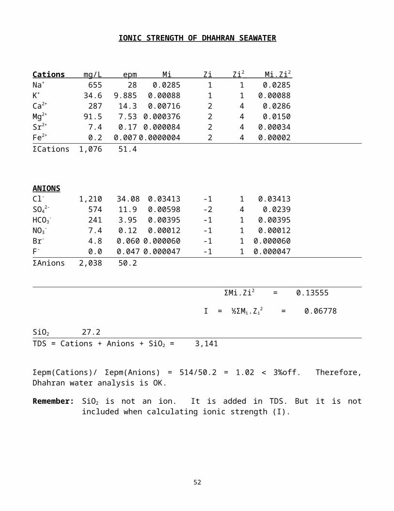
IONIC STRENGTH OF DHAHRAN SEAWATER

Cations mg/L epm Mi Zi Zi 2 Mi.Zi 2 Na+ 655 28 0.0285 1 1 0.0285K+ 34.6 9.885 0.00088 1 1 0.00088Ca2+ 287 14.3 0.00716 2 4 0.0286Mg2+ 91.5 7.53 0.000376 2 4 0.0150Sr2+ 7.4 0.17 0.000084 2 4 0.00034Fe2+ 0.2 0.007 0.0000004 2 4 0.00002ΣCations 1,076 51.4

ANIONSCl- 1,210 34.08 0.03413 -1 1 0.03413SO4

2- 574 11.9 0.00598 -2 4 0.0239HCO3

- 241 3.95 0.00395 -1 1 0.00395NO3

- 7.4 0.12 0.00012 -1 1 0.00012Br- 4.8 0.060 0.000060 -1 1 0.000060F- 0.0 0.047 0.000047 -1 1 0.000047ΣAnions 2,038 50.2

ΣMi.Zi2 = 0.13555

I = ½ΣMi.Zi2 = 0.06778

SiO2 27.2TDS = Cations + Anions + SiO2 = 3,141

Σepm(Cations)/ Σepm(Anions) = 514/50.2 = 1.02 3%off. Therefore, Dhahran water analysis is OK.

Remember: SiO2 is not an ion. It is added in TDS. But it is not included when calculating ionic strength (I).

40

Properties of Saline WaterM.H. Sharqawy, J. H. Lienhard, and S. M. Zubair, "Thermophysical properties of seawater: A review of existing correlations and data,

Desalination and Water Treatment 16 (2010) 354–380

DESCRIPTIONThis page provides tables and a library of computational routines for the thermophysical properties of seawater including:

Density

Specific heat capacity

Latent heat of vaporization

Thermal conductivity

Dynamic viscosity

Surface tension

Vapor pressure

Boiling point elevation

Specific enthalpy

Specific entropy

Osmotic coefficient

These properties are those needed for design of thermal and membrane desalination processes. They are given as functions of temperature and

salinity. The pressure is taken as atmospheric pressure (0.1 MPa) up to the saturation temperature and at saturation pressure for higher

temperatures. The temperature and salinity ranges are 0 - 120 degC and 0 - 120 g/kg respectively.

Details about the source, validity and accuracy of each property function can be found in:

Mostafa H. Sharqawy, John H. Lienhard V, and Syed M. Zubair, "Thermophysical properties of seawater: A review of existing correlations and

data," Desalination and Water Treatment, 2010, in press.

The seawater properties library routines are available in MATLAB and EES formats. They are a self contained library and are extremely easy to

use. They will run on all computers that support MATLAB and EES.

This software is provided "as is" without warranty of any kind. See the file sw_copy.m for conditions of use and licence.

DOWNLOADS Tables of properties in pdf format

MATLAB files in a zip archive

EES library file in a zip archive

INSTALLATIONFor MATLAB:

Place all the MATLAB m files in a directory called "Seawater"

Add this folder to the MATLAB search path. See the MATLAB command "help path" for more details.

For EES:

Place the file SEAWATER_EES.LIB in a directory called "Seawater"

41

Place this folder inside the Userlib folder of EES. See the EES library routines for usage of the properties functions.

42

PROPERTY FUNCTIONSProperty (unit) Temperature, T (degC) Salinity, S (g/kg) Function name

Density, (kg/m3) 0 - 180 0 - 160 SW_Density(T,S)

Specific heat capacity, (J/kg.K) 0 - 180 0 - 180 SW_SpcHeat(T,S)

Thermal conductivity, (W/m.K) 0 - 180 0 - 160 SW_Conductivity(T,S)

Dynamic viscosity, (kg/m.s) 0 - 180 0 - 150 SW_Viscosity(T,S)

Surface tension, (N/m) 0 - 40 0 - 40 SW_SurfaceTension(T,S)

Vapor pressure (kPa) 0 - 200 0 - 240 SW_Psat(T,S)

Boiling point elevation (K) 0 - 200 0 - 120 SW_BPE(T,S)

Latent heat of vapori. (J/kg) 0 - 200 0 - 240 SW_LatentHeat(T,S)

Specific enthalpy (J/kg) 10 - 120 0 - 120 SW_Enthalpy(T,S)

Specific entropy (J/kg.K) 10 - 120 0 - 120 SW_Entropy(T,S)

Osmotic coefficient 0 - 200 10 - 120 SW_Osmotic(T,S)

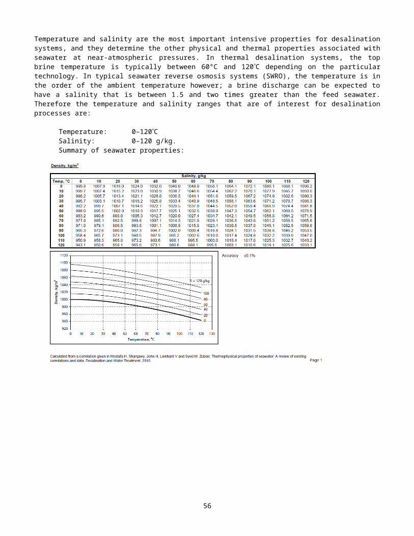
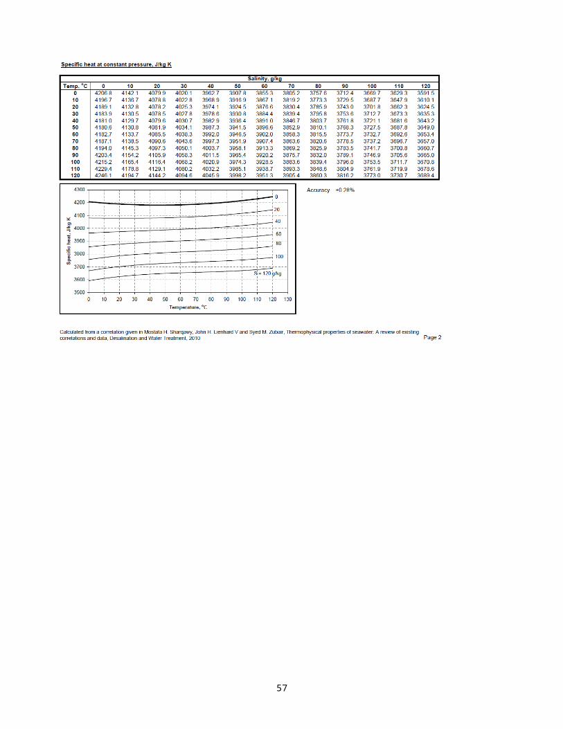
3.2 Thermophysical Properties Of Seawater

Source: www.deswater.com doi no. 10.5004/dwt.2010.1079

The knowledge of seawater properties is important in the development and design of desalination systems. Most of the data are presented as tabulated data, which require interpolation and extrapolation to conditions of interest, and not all desirable properties are given in any single source, particularly transport properties such as viscosity and thermal conductivity.

As a first approximation, most physical properties of seawater are similar to those of pure water, which can be described by functions of temperature and pressure. However, because seawater is a mixture of pure water and sea salts, salinity (which is the mass of dissolved salts per unit mass of seawater) should be known as a third independent property in addition to temperature and pressure. Differences between pure water and seawater properties, even if only in the range of 5 to 10%, can have important effects in system level design: density, specific heat capacity, and boiling point elevation are all examples of properties whose variation affects distillation system performance in significant ways. Therefore, it is necessary to identify accurately the physical and thermal properties of seawater for modeling, analysis, and design of various desalination processes.

Temperature and salinity are the most important intensive properties for desalination systems, and they determine the other physical and thermal properties associated with seawater at near-atmospheric pressures. In thermal desalination systems, the top brine temperature is typically between 60°C and 120C depending on the particular technology. In typical seawater reverse osmosis systems (SWRO), the temperature is in the order of the ambient temperature however; a brine discharge can be expected to have a salinity that is between 1.5 and two times greater than the feed seawater. Therefore the temperature and salinity ranges that are of interest for desalination processes are:

Temperature: 0–120CSalinity: 0–120 g/kg.Summary of seawater properties:

43

44

45

File: Sharqawy et. el. Seawater properties -DWT-16-354-2010.pdfTotal Pages 28

46

47

48

49

50

51

52

53

54

55

56

57

58

59

60

61

62

63

64

65

66

67

68

69

70

71

72

73

74

75

76

77

78

79

80

81

82

83

84

85

86

87

88

89

90

91

92

93

94

95

96

97

98

99

100

TOPIC 4

OVERVIEW OF VARIOUS DESALINATION PROCESSES

In this section, we will cover the following desalination processes:

1. Multi-Stage-Flash (MSF)

2. Multi-Effect (ME) Distillation, Multi-Effect Boiling (MEB)

3. Vapor Compression

4. Electrodialysis (ED)

5. Reverse Osmosis (RO)

6. Solar desalination (This method will be covered toward the end of the course)

HISTORY OF DESALINATION

Desalination technology is not a new concept.  Desalination has been used for thousands of years, such as

Greek sailors, boiling water to evaporate fresh water away from the salt and

Romans using clay filters to trap salt.

Up to the year1800 desalination was practiced on ship boards. The process involved using single stage stills operated in the batch mode. The equipment and product quality varied considerably and were dependent on the manufacturer and operator. Mist carryover was always a problem.

101

In year 1912, a six effect desalination plant with a capacity of 75 m3/d was installed in Egypt.

In year 1957, the landmark of the four-stage flash distillation plant by Westinghouse was installed in Kuwait.

The MSF patent by Silver gives a major advancement over the Westinghouse configuration because of the much smaller specific heat transfer area for the condenser tubing. This reduced considerably the capital cost since the high tubing cost in the Westinghouse system was replaced by inexpensive partitions in the MSF systems.

1960 First MSF plants commissioned in Shuwaikh, Kuwait and in Guernsey, Channel Island. The MSF unit in Shuwaikh had 19 stages, a 4550 m3/d capacity, and a performance ratio of 5.7.

.

102

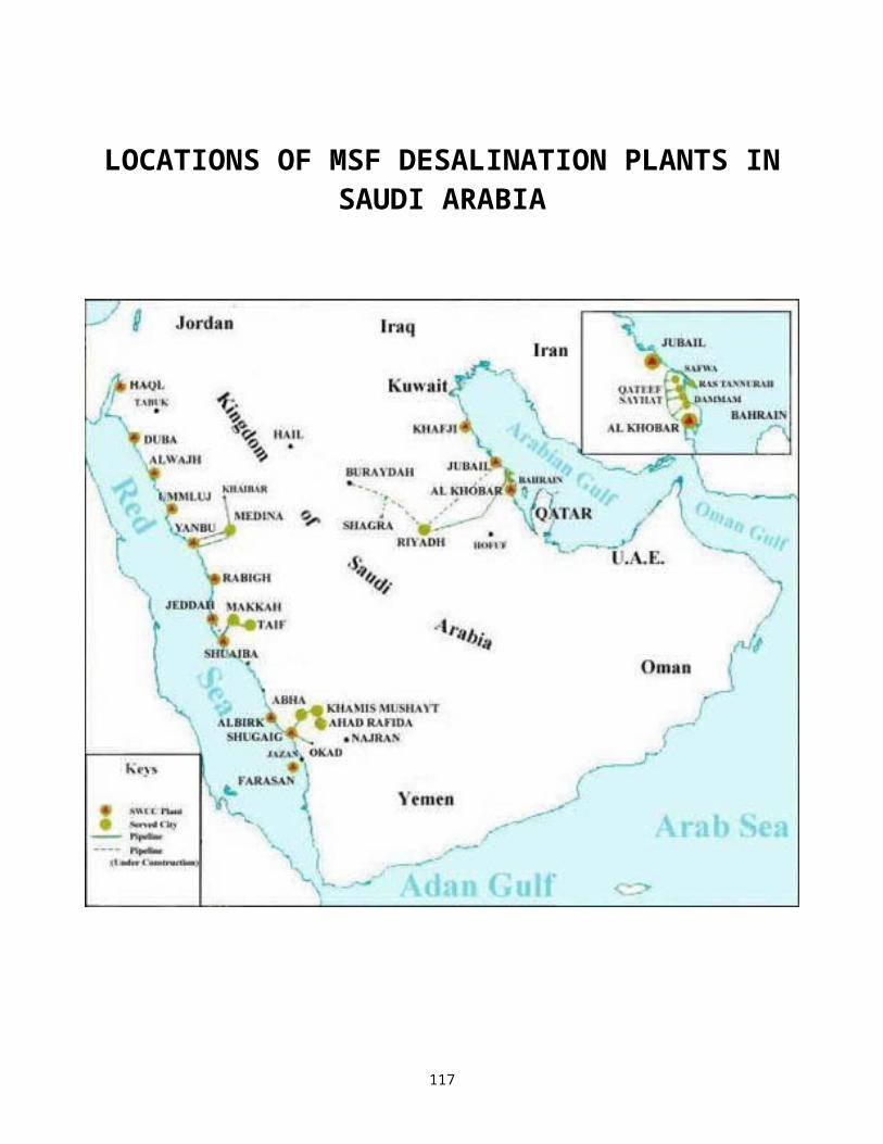
LOCATIONS OF MSF DESALINATION PLANTS IN SAUDI ARABIA

103

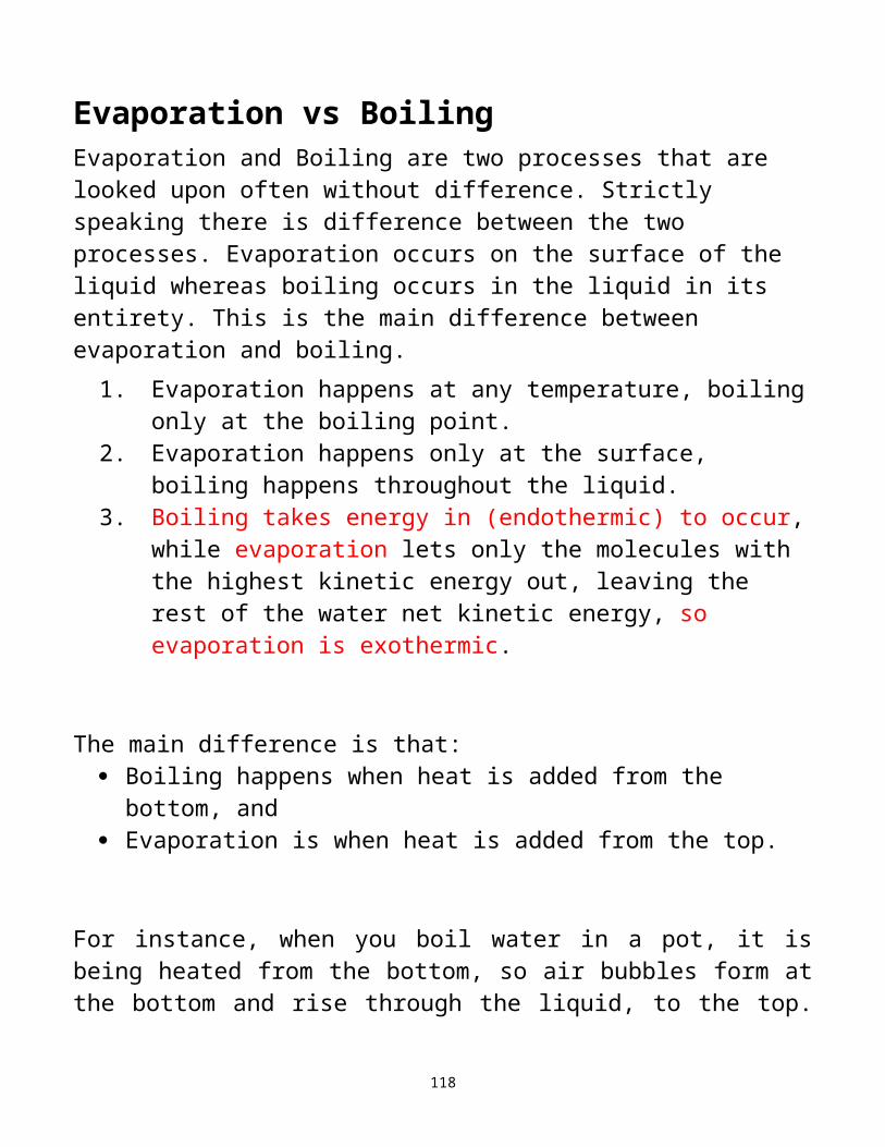
Evaporation vs BoilingEvaporation and Boiling are two processes that are looked upon often without difference. Strictly speaking there is difference between the two processes. Evaporation occurs on the surface of the liquid whereas boiling occurs in the liquid in its entirety. This is the main difference between evaporation and boiling.

1. Evaporation happens at any temperature, boiling only at the boiling point.

2. Evaporation happens only at the surface, boiling happens throughout the liquid.

3. Boiling takes energy in (endothermic) to occur, while evaporation lets only the molecules with the highest kinetic energy out, leaving the rest of the water net kinetic energy, so evaporation is exothermic.

The main difference is that: Boiling happens when heat is added from the bottom, and Evaporation is when heat is added from the top.

For instance, when you boil water in a pot, it is being heated from the bottom, so air bubbles form at the bottom and rise through the liquid, to the top. It would be evaporation if the heat was added from the top (no bubbles would form).

There is difference between the two states in terms of the time taken too. Boiling takes place very quickly and swiftly too. On the other hand evaporation takes place slowly and gradually. This is a very important difference between the two processes.

It is interesting to note that the boiling point is reduced when the pressure of the surrounding atmosphere is reduced.

104

Single Stage Evaporation Process

105

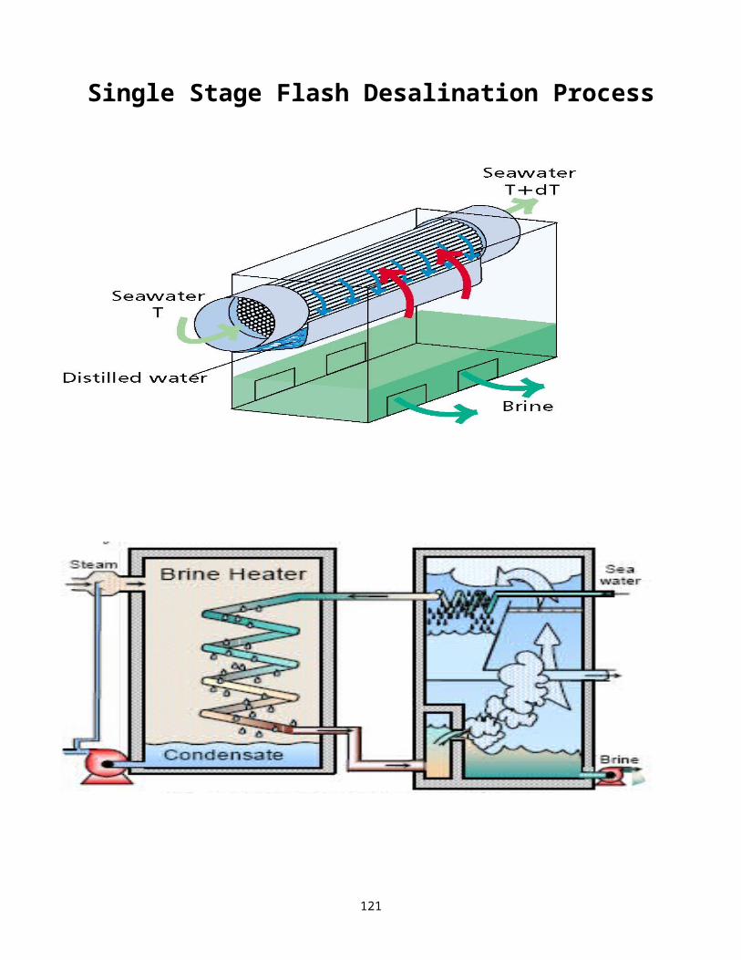
Single Stage Flash Desalination Process

Multiple Stage Flash Desalination Processes

106

ONCE-THROUGH FLASH DESALINATION PLANT

FLASH DESALINATION PLANT WITH BRINE RECYCLING

107

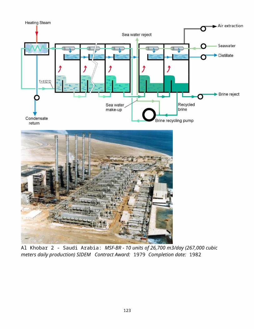
Al Khobar 2 - Saudi Arabia: MSF-BR - 10 units of 26,700 m3/day (267,000 cubic meters daily production) SIDEM Contract Award: 1979 Completion date: 1982

108

MSF plant at Jubail 0.880 million m3/day

109

3.3 SHOAIBA DESALINATION PLANT, SAUDI ARABIA

The finished desalination plant currently ranks as the largest in the world and uses multi-stage flash (MSF) distillation

Product water output: 74,000m³/day (Phase 1); 450,000m³/day (Phase 2)

110

1.

3.4

3.5 WORLD’S LARGEST DESALINATION PLANT GOES ON STREAM IN RAS AL-KHAIR

 RAS AL-KHAIR – Minister of Water and Electricity Abdullah Al-Hussayen commissioned the first phase of world’s largest desalination project here on Tuesday. Ras Al-Khair plant exceeds 80 percent, and it is expected to start producing water before the end of the first quarter of 2014.

The plant for production and pumping of desalinated water and generation of electricity is located in the Ras Al-Khair Industrial City, 75 km north-west of Jubail. The plant is set to generate 15,000 jobs.

Al-Hussayen, who is also chairman of the SWCC board, said that the project, which is estimated to cost a total of more than SR27 billion, consists of the largest desalination pumping plant ever built in the history of SWCC.

“The plant has the production capacity of 1.025 million cubic meters of desalinated water per day and electricity production capacity of 2,600 MW. The plant will supply 1,350 MW of electricity to Maaden, and 1,050 MW to Saudi Electricity Co., in addition to 200 MW to be used within the plant,” he said.

111

A total of 800,000 cubic meters of water will be supplied to Riyadh city. It will be capable of serving about 3.5 billion people in the city of Riyadh.

Another 100,000 cubic meters to Al-Washm, Sudair, Majma, Al-Zulfi and Al-Ghat regions.

A total of 100,000 cubic meters will be supplied to the regions located north of the Eastern Province, including Hafar Al-Batin, Qaisoomah, and Qaryat Al-Olya.

The desalination plant will comprise of eight MSF units and 17 RO units. The MSF units will have a capacity to produce 160 MIGD while the RO units will produce 68 MIGD. Three of the MSF units were built at Doosan Heavy Industries Vietnam, while the other five were built at Doosan Korea facility.

112

Multi-Stage-Flash (MSF) Desalination Process

Description of the MSF Desalination Process with Brine Recycling

The simplified flow diagrams of an MSF process are shown in Fig. 4.1 and 4.2. The plant consists of three main parts namely, the heat input section (brine heater), the heat recovery section, and the heat reject section. The process itself can be described in terms of three streams: seawater stream, recycle brine stream, and distillate stream.

The intake seawater pumps deliver the filtered and chlorinated seawater to the tube side of the last stage (in Fig. 4.2, 17th stage) from where it flows in cross flow pattern through tubes of the last three stages of the reject section, effecting condensation of the flashing vapor on the outside of these tubes. After the seawater leaves tube bundles of the reject section, it is split up; a portion is discharged to the sea, and the remainder becomes the make-up feed for the MSF plant.

To control scale, the make-up water is treated with an acid in which case it is called an acid treatment plant, or with a scale inhibitor chemical in which case it is called an additive treatment plant. Most modern plants, whether acid or additive dosed, have de-aerator to remove up to 95% of O2. The gases, stripped by the stripped by the steam, are led to the shell side of the pre-condenser which is cooled externally by the seawater.

The treated feed is sprayed into the last flash stage which is maintained at the lowest temperature and highest vacuum (e.g. 42 °C and 27.6 in. vac.). A substantial portion of the non-condensable gases is driven off in the last stage which is vented directly to the pre-condenser. This helps minimize O2

corrosion by minimizing its concentration in the brine.

The make-up feed mixes with the unvaporized brine in the last stage and the sum-total is taken up by the recycle brine

pump and introduced to the tube side of the last (i.e. 14 th) stage of the recovery section. The brine flows through tubes of the entire heat recovery section, being pre-heated by the condensing vapor and the re-flashing distillate.

After the pre-heated brine comes out of the tube bundles of the recovery section, its final heating is done in the heat input section (brine heater) by means of steam drawn either from a boiler (single-purpose desalination plant), or as extraction/back pressure steam from a steam turbine (dual-purpose power-desalination plant). The brine exits the brine heater at the desired top brine temperature (TBT) and is dumped into the first flash chamber. Here the prevailing pressure is such that the actual temperature of the entering brine is higher than its saturation temperature. A fraction of the supersaturated brine thus flashes off to vapor which passes through the demisters near the ceiling of the flash stage and condenses on the outside of the cooler tube bundle of the first stage, thereby giving up its latent heat of condensation. The brine inside the tube bundle is pre-heated and the vapor is condensed and collected in the so-called distillate tray installed beneath the tube bundle. The gases including CO2 and O2 still in the brine are led along with some water vapor to the inter-condenser for removal.

The brine from the first stage then enters through an orifice into the second stage where more brine flashes off to vapor which, by condensing on the cooler overhead brine-carrying tubes, pre-heats the brine and produces more distillate. This flashing process continues from stage to stage at progressively lower temperatures until the brine reaches the last sage and the cycle is repeated.

The distillate produced in each stage joins with that from the previous stages and flows on to the next stage. The total distillate from the last stage (which is under vacuum) is withdrawn by a pump. Total dissolved solids (TDS) of the distillate are typically 30 ppm.

1. Single-Purpose vs. Dual-Purpose MSF Plant :

2

The single-purpose plant has its own steam producing boiler. The entire capital, energy, and operating costs of steam generating plant are, therefore, allocated to the MSF water plant.

In a dual-purpose power-water plant the steam produced in the steam producing plant is shared between the power & water plants. The capital, energy, and operating costs of steam generating plant are also shared between the power & water plants. As a result, the cost of water is lower than that produced by a single-purpose water plant.

2. Low Temperature (LT) vs. High Temperature (HT) Plants : MSF plants with top brine temperature (TBT) of 85-90 oC at the brine heater outlet are known as LT while those with TBT>90 oC are called HT plants. In the Gulf region these days most MSF plants are designed for dual temperature operation. In winter months when the water demand is low, these plants are operated in the LT mode. To produce more water in the summer months, they are operated in the HT mode, ranging from 100o to 113 oC TBT.

3. Acid-Dosed vs. Additive-Dosed Plants : All MSF plants are operated at top brine temperatures ranging from 85o to 112oC. At these temperatures, there is no potential for calcium sulfate scale to form. But the potential to form alkaline scale (CaCO3 & Mg(OH)2) exists.

When acid (usually sulfuric) is injected to seawater make-up, the plant is known as acid-dosed. Acid completely destroys the alkalinity from the feed water so that the acid-dosed plants can be operated in the HT mode where they are thermally more efficient.

When chemical additives are injected to inhibit the alkaline scale, the plants are called additive-dosed. These days scale inhibitors are available which permit plant operation up to 113 oC. The two modes of scale inhibition are compared in the following:

3

● Acid-dosed plants are thermally more efficient due to better heat transfer but more prone to corrosion;

● Additive-dosed plants are thermally less efficient but also less prone to corrosion;

● Additive treatment is cheaper;● The useful life of an additive plant is longer (>20 years)

than an acid plant.

4. Temperature Rise Through Brine heater (∆T n): Temp. by which brine is heated in the brine heater as a result of steam condensing on the outside of the tubes.

4

5

6

For a given recycle brine flow rate (MR),

greater the flash range ( Tf); higher the distillate output (MD)

7

Figure 4.1 Process flow diagram of MSF plant [1]

8

MSF DESALINATION UNIT AT GHAZLAN POWER PLANT

9

Figure 4.2 Block flow diagram of MSF unit at Ghazlan power plant

Figure 4.3 Block flow diagram of MSF unit at Jeddah-II power & desal plant

10

SOME CALCULATIONS FOR MSF DESAL UNIT AT GHAZLAN POWER PLANT

MULTI-STAGE-FLASH (MSF) DESALINATION PROCESS

DATA FOR GHAZLAN MSF PLANT

(Refer to the accompanying Line Diagram, Fig. 3.2).

Mass flow rate % Seawater (MSW) = 1,179,138 Kg/h

Seawater Discharge (MSWO = 796,689

Feed Make-up (MF) = 382,449

Recycle Brine (MR) = 1,302,721

Brine Blow down (MB) = 244,354

Distillate (MD) = 138,095

Super-Heated Steam (MSS) = 23,038

Desuper-Heating Water (MDW) = 771

Condensate (MC) = 23,809

Total Dissolved Solids of Feed (XF) = 50,000 mg/l

Recycle Brine (XR) = 70.000

Blow-Down (SB) = 78,250

Distillate (SD) = 5

Seawater pH = 8.1

Recycle Brine pH

For Acid – Dosed = 7.2 – 7.6

For Additive – Dosed = 8.7

11

1. Gained output ratio (GOR)

2. Performance Ratio (PR)

= 6.1 Kg/2325 kJ = 6.1 lbs./1000 BTU

= 11.0 Kg/1000 Kcal

12

TEMPERATURES

Seawater Inlet (TSWi) = 35 oC

Outlet (TSWo) = 46.1

Recycle Brine Inlet (TR) = 46.1

Feed Make-up (TF) = 46.1

Brine Blow-Down (TB) = 46.1

Last Stage or Bottom Brine (TB) = 46.1

Distillate (TD) = 43.9

Super-Heated Steam (TSS) = 162.8

Saturated Steam (TS) = 120

Condensate (TC) = 120

Desuper – Heating Water (TDW) = 120

HEAT TRANSFER DATA FOR GAZLAN DESAL UNIT

S.No.

Parameter Units Brine HTR.

Heat Recovery

1. No. of Stages - 1

2. Tube O.D. m 0.01585 0.01585

3. Tube I.D. m 0.01445 0.01257

4. Total No. of Tubes (N) - 1228 1680 Per Stage

5. No. of Tubes in Vertical Tier (Nv)

- 18 25

6. Total Surface Area (A) m2 397.95 3992.84

7. Tube Thermal Cond. (KW) Kj/h.m.oC

61.24 172.82

8. Fouling Factor (FF) h.m2.oC/Kj

0.0376X10

0.0269X10

9. Design H.T. Coeff. (UD) Kj/h.m.oC

11,120 11,446

10. Brine Velocity Thru. Tubes (Ub)

m/sec. 1.729 1.668

13

14

15

16

TOPIC 4b

OVERVIEW OF VARIOUS DESALINATION PROCESSES

4.2 MULTI-EFFECT DISTILLATION (MED) process

4.2.1 Description of the MED Process:

The simplified flow diagram of an MED process is shown in Fig. 4.3. In ME vapor from the first evaporator condenses in the second and the heat from its condensation serves to boil the salt water in the latter. Therefore, the second evaporator acts as a condenser for the vapor from the first and the task of this vapor in the second evaporator is like that of the heating steam in the first. Similarly the third evaporator acts as a condenser for the second, and so on. This principle is illustrated in Fig. 4.3. Each evaporator in such a series is called an effect.

Obviously the boiling temperatures (and pressures) in the different evaporators cannot be the same. Consider, for instance, the boiling process in the first evaporator. The heating steam is at a pressure of 1 atm; hence it condenses at 100°C. If the pressure in the vapor space of the first evaporator were also 1 atm, the corresponding boiling temperature for seawater would be about 100.53oC, and the heat of condensation could not flow to the boiling seawater since it would be at a higher temperature than the condensing steam. It is necessary to maintain reduced pressure in the vapor space of the first evaporator in order to make up for the difference of the boiling temperatures of pure water and salt water. This alone is not enough. To maintain reasonable heat flow rates across the tubes from the condensing steam to the boiling seawater, the temperature of the seawater must be at least several degrees lower than that of the condensing steam. If the boiling temperature of seawater in the first evaporator is to be 95°C, the pressure in the vapor space of the first evaporator must be maintained at 0.82 atm. At this pressure the vapor will condense in the second evaporator at 94.5°C, and we wish to maintain the salt water at a boiling temperature of 90°C to provide again a reasonable temperature difference across the walls of the tubes of the second evaporator.

Since the pressure in all evaporators is less than atmospheric, pumps P (Fig. 4.3) must be provided to deliver the fresh product and the rejected brine at atmospheric pressure. The fresh water of each effect is pumped to atmospheric pressure by a separate pump. Alternatively the fresh water is flashed between the effects in small flash chambers where the vapor joins that entering the next effect.

Provision must also be made for the removal of air and other noncondensing gases from the vapor spaces of the evaporators. If these gases were allowed to accumulate, the pressures in the vapor spaces over the boiling liquids would soon rise to levels that can stop the boiling processes. The vapor space of each evaporator may be connected to a steam ejector or a vacuum pump to get rid of the non-condensables and maintain the appropriate pressure. Instead of this arrangement, it is also possible to connect all the vapor spaces in series through throttle valves and only the last one to a steam ejector or a vacuum pump. The latter method is possible where the amount of air is small. It causes less vapor loss with the non-condensable gases than the first.

17

Figure 4.3. Multi-effect-desalination (MED) process diagram.

18

In a real ME plant, the seawater feed introduced on the tube side of the 1st effect is not at ambient temperature but is first pre-heated by using it as cooling water in the Condenser (Fig. 3.3) where it picks up heat from the condensing vapor from the 4 th effect & also by passing it through a plate type heat exchanger in which it picks up heat from the brine and distillate streams.

4.2.2 Optimum Number of Effects:

Theoretical GOR = 1 per Effect

That is, in each effect 1 kg of distillate can be produced by condensing 1 kg of heating steam.

Practical GOR 0.8 per Effect

Therefore, from a 4-effect MED plant, GOR 3.2 from a 10-effect MED plant, GOR 8

Cost of an MED plant is dictated by its initial capital cost and operating cost (especially the cost of heating steam). Greater the number of effects in an MED plant, greater is its thermal efficiency. But greater the number of effects, greater is the initial investment. The optimum number of effects is given by the following eq.

(4.15)

where: Nopt = Optimum no, of effects S = Cost of heating steam A = Capital cost of each effect

Clearly, Greater the capital cost, lower the no. of effects Greater the cost of heating steam, greater the no. of effects.

19

4.2.3 MED vs. MSF

1. In MED process, boiling of sea water takes place inside the tubes whereas in MSF the brine is only heated (single phase) inside the tubes; the flashing takes place outside the tubes. Since boiling heat transfer coefficients are much higher than single phase coefficients, MED is thermally superior to MSF.

2. With MED, high GOR are possible. For example, a l0-effect :MED plant will yield a GOR of about 10 whereas in MSF, 15 to 30 flash stages will be required to obtain GOR of l0.

3. Uniform feed distribution in an MED process is a serious problem. Because of uneven distribution of seawater inside the tubes, dry-out occurs, leading: to serious scale formation

The current tendency is to restrict the top brine temp. (TBT) to about 60°C which considerably minimizes the chances of scale formation.

4.2.4 Horizontal Tube Multiple Effect (HTME) Process

This is a variation of MED process in which (1) the heat transfer tubes in each effect are arranged horizontally, and (2) the steam/vapor are condensed inside the tubes while the pre-heated seawater feed is sprayed on the outside of the tubes (Figure 3.4). In this process, scale can be visually observed and easily removed by turning off the steam and circulating cold seawater. The scale cracks up. Also, HTME is thermally even more efficient than the MED process.

Figure 4.4. Horizontal tube multi effect (HTME) process diagram.

20

4.3 VAPOR COMPRESSION (VC) DESALINATION PROCESS

4.3.1 Basis of Vapor Compression:

Suppose that in a single effect evaporator, saturated heating steam at 105°C is used to boil brine at 100oC, and the vapor produced at 100°C is condensed as distillate. If, however, the vapor produced at 100°C were compressed, both its pressure and temperature could be raised to those of the heating steam. That is, its temperature could be raised to 105oC. In such a case, the compressed vapor could be used as a· source of heat, instead of the prime heating steam. Since compression energy is much less than the thermal energy in the form of latent heat of prime steam therefore, VC process is even more efficient than the MED process.

4.3.2 Description of the VC Process:

The simplified flow diagram of a VC process is shown in Fig. 4.5.

While MED and flash-evaporation units use an external supply of heating steam as the primary heat source, vapor compression distillation, often shortened to "compression distillation", uses literally its own steam, after it has been compressed, as a heat source. In this method the energy requirement per unit of fresh water product appears lower than that of the heat-driven processes, but it is necessary to provide the energy required as shaft work (100% available energy), as shown in Fig. 4.5.

In the vapor compression unit of Fig. 4.5, seawater preheated in a tubular heat exchanger by the outgoing streams of brine and fresh water boils outside the tubes of an evaporator-condenser. The vapor released is compressed and led back to condense inside the tubes, thus providing the heat necessary for the boiling process. The noncondensing gases are withdrawn from the steam condensation space by a simple vent if the pressure is above atmospheric or by a vacuum pump if the pressure is below atmospheric. An electric heater, or another heat source, e.g., an initial supply of steam is needed to start the system. The long-tube evaporator was first used with the vapor compression systems. The horizontal spray film type (Fig. 3·6) is now preferred because of its relatively higher overall heat-transfer coefficient, particularly under high vacuum, its more effective venting, its larger vapor release surface and its convenience in observing the surface conditions of the tubes.

The heart of the installation is the compressor. If the vapor were not compressed, it could not condense because the condensation temperature of pure vapor is less than the boiling temperature of the salt water at the same pressure. For instance, if the vapor pressure is 1 atm, water vapor condenses at 100oC, but doubly concentrated seawater boils at about 101oC. In order to make the vapor condense at 101oC, it is necessary to compress it to at least 1.03 atm.-

The type of conventional vapor compressor depends on the size of the distiller as well as the vapor pressure, which is related to its temperature. A positive displacement compressor, usually a Roots blower, driven by an electric motor or an engine at speeds of 500-2500 rpm, is suitable for capacities up to 500 t/d when operating at atmospheric pressure.

A centrifugal compressor running at speeds of 5000-20,000 rpm is used for capacities up to 2000 t/d. Operation is usually sub-atmospheric (70-90oC) to reduce scale problems. For lower temperatures the compressor is like a high-head blower (such as that used in the direct freezing process), since for the same temperature difference the change in corresponding vapor pressure becomes smaller as the temperature is lowered and hence the power requirement. For capacities larger than 2000 t/d, even for operation at

21

atmospheric pressure, it may be necessary to use very high volumetric flow compressors such as axial-flow compressors which have not yet been sufficiently developed for distillation applications.

A simpler type of compressor is the steam-ejector compressor (known as a thermo-compressor). The available energy of high-pressure superheated steam is utilized directly in an ejector as a compression device. This type has the advantage of having no moving parts but is much less efficient than the mechanical vapor compressor. Thermo-compressor units are usually designed for capacities up to 500 t/d and for operation at a temperature 50°C and lower to avoid scale problems. They produce at best 3-5 kg distilled water per kg of high- or medium pressure superheated steam (10-60 atm).

4.3.3 Mechanical Vapor Compression (MVC) vs. Thermal Vapor Compression (TVC)

As indicated before, the vapor in a VC process can be compressed either by a compressor in which case it is known as mechanical vapor compression (MVC) or by using a steam jet ejector which is called thermal vapor compression (TVC). Steam jet ejectors have no moving parts and are accordingly very reliable. Off-shore rigs use TVC units on account of their reliability, but thermally they are much less efficient as is evident from the following.

VC Process PR (lbs/1000 Btu)

1. Mechanical Vapor Compression 14

2. Thermal vapor compression or Steam Ejector 2-3

22

MECHANICAL VAPOR COMPRESSION

Figure 4.5. Mechanical Vapor compression (MVC) process diagram

The Vapor Compression Systems produce 1500 Gallons (5700 litres) or 3000 Gallons (11340 litres) per day and are extremely energy efficient. Norland has effectively and successfully designed a system that produces high-quality, distilled water (less than 1 ppm TDS) at the lowest possible cost. Spectrum Vapor Compression Systems from Norland offer the following features:

Easy Installation.

Solid State operational controls.

Minimal preventive maintenance.

Dependable and Durable.

Low Operational Costs. (Electricity will cost less than $0.01/gallon).

Up to 98% less waste water used than on other models.

Up to 3,000 gallons (11,340 litres) per day.

23

Figure 4.5a. Mechanical Vapor compression (MVC) process diagram.

24

4.4 MULTI-EFFECT BOILING (MEB) VAPOR COMPRESSION (VC)

Compared with single effect evaporator, the single effect VC system has far better performance ratio (PR), 2-3 for TVC and 14 for MVC vs. 0.8 for the single-effect. By using multiple-effects in the VC plant, both the PR and distillate output can be increased. In Figure 4.6 the VC plant consists of 4-effects.

Seawater at 33 oC is used as a coolant in the final condenser built in the last (4th) effect. Part of the vapor produced in the 4th effect is condensed as distillate. The remainder of the vapor is taken to the steam jet ejector where high pressure steam at 353 psi (24 atm.a) is used to raise its temperature to ≈ 63 oC. This vapor is used as the heating medium in the 1st effect. The seawater from the final condenser is split. A part of it (at 44oC) is used as feed to all 4 effects. The feed is sprayed on the outside of the heat transfer tubes which are horizontally arranged. The top brine temp. (TBT) in the 1st effect is < 60 oC which minimizes the scale deposit.

The unit has a diesel-fired boiler which supplies steam at the start-up. Once the plant reaches steady state, the steam supply from the boiler is cut off. The unit is capable of producing 1.2 US million gallons per day (USMGD) of distillate. Its PR is 8 and it is 35% cheaper than an MSF plant of same size. However, whereas single MSF units as large as 15 USMGD are operating in the Gulf region, the largest MED units so far operating in Sharjah are 6 USMGD size.

Figure 4.6. Multi-effect boiling (MEB) thermal vapor compression (TVC) horizontal spray film.

25

MED PLANTS IN GCC COUNTRIES

Location No. of Capacity ea Total Year Supplier

Units Unit (MGD) (MGD)

• Ras Tanura Refinery(Aramco) 4 0.66 2.64 • Safaniya Gas Plant (Aramco) 2 0.66 1.32 • Ras Tanajib Gas Plant (Aramco) 2 0.50 1.00 • Jeddah Refinery (Aramco) 2 0.66 1.32 • Rabigh Refinery (Project) 2 1.32 2.64 • Dalma (Abu Dhabi) 1 1.2 1.20 1996 Sidem • ALBA (Bahrain) 4 2.84 11.40 2001 Technip • Umm AI-Nar (Abu Dhabi) 2 4.20 8.40 2000 Sidem • AI-Taweelah AI (Abu Dhabi) 14 4.53 63.40 2002 Sidem • Layyah (Sharjah) 2 6.00 12.00 2001 Sidem·

26