CHARLES STANLEY LASOTA - DTIC · CHARLES STANLEY LASOTA S ,AUGU• 3 191 B.S., Electrical Engineering University of Kansas, 1985 Submitted to the Departments of Nuclear Engineering

AD-A268 704 ,

.__ctivity Estimation and Validationfor the Control of Reactor Neutronic Power

by 4DTICELECTE

CHARLES STANLEY LASOTA S ,AUGU• 3 119B.S., Electrical EngineeringUniversity of Kansas, 1985

Submitted to the Departments of Nuclear Engineering and Electrio Engineering andComputer Science in Partial Fulfillment of the Requirements for the Degrees of

Master of Science in Nuclear Engineeringand

Master of Science in Electrical Engineering and Computer Science

at theMassachusetts Institute of Technology

May 1993

0 Charles Stanley LaSota, 1993. All Rights reserved. The author hereby grants to MITand the US government permission to reproduce and to distribute publicly copies of thisthesis document in whole or in part.

Signature of Author _ _ ___ __

Certified bySDr. Joho(A. Bernard, Jr., MIT NIt, Thesis Co-Advisor

ftCertified byDav•d D. Lanning, Prof ssor of Nuclear Vngineering, Thesis Co-Advisor

.- I k- /

Certified by ,z Z CDr. Marija lic', SeniorkeFe Scienti" es R

Department of E1 -t -Cal Comp er Science

Accepted by : \

Carf earl air, EtC/Com on Graduate Students'"

Accepted by _ n t/,'r t

Allan F. Henry, Chairman, NED)Committee on Graduate Students

93-20147a35 q ~ i ooi 11111q III I ll III I n,

THIS DOCUMENT IS BEST

QUALITY AVAILABLE. THE COPY

FURNISHED TO DTIC CONTAINED

A SIGNIFICANT NUMBER OF

PAGES WHICH DO NOT

REPRODUCE LEGIBLY.

Reactivity Estimation and Validation for the

Control of Reactor Neutronic Power

by

Charles Stanley LaSota

Submitted to the Departments of Nuclear Engineering and Electrical Engineeringand Computer Science on the 7th of May 1993 in partial fulfillment of the requirementsfor the degrees of Master of Science in Nuclear Engineering and Master of Science inElectrical Engineering and Computer Science.

Abstract

From July 1986 to July 1991, a joint MIT-SNL research team developed acontroller capable of safely raising reactor power by approximately five orders ofmagnitude in a few seconds. This controller was experimentally demonstrated on the MITResearch Reactor (MITR-fI) as well as on the Sandia National Laboratories' Annular CoreResearch Reactor (ACRR). This controller's intended application is for the control ofspacecraft nuclear reactors. However, it also has direct application for the control ofmilitary, commercial, and research reactors.

This report is concerned with a method for enhancing the controller's performancethrough the development of an improved model to validate estimates of the magnitude ofreactivity feedback effects. The focus is on the Doppler effect but the resulting model isapplicable to other types of reactivity feedback such as that associated with the thermaleffects of a hydrogen coolant. The specific accomplishments of this report include:

1. The development of a reactor model that generates analytic values of reactivityresulting from reactor temperature variation.

2. The development of an adaptive estimation routine to correct deficiencies in thereactor model so that the model generates the validated estimate of reactivity inreal time. (Note: For the purpose of this report the inverse kinetics estimate ofreactivity is assumed to be correct).

3. Application of a parity space approach to provide for validation of assumedindependent reactivity inputs.

2

4. Performance of system analysis to determine the minimum number of sensor inputsto implement the closed form control laws and still allow for automated faultdiagnosis.

5. Demonstrations of the adaptive estimation routine for reactivity.

Thesis Co-Advisor: Dr. John A. Bernard Jr.

Title: Director of Reactor Operations

Thesis Co-Advisor: Professor David D. Lanning

Title: Professor of Nuclear Engineering

Thesis Reader: Dr. Marija Ilic'

Title: Senior Research Scientist,Department of Electrical Engineering and Computer Science

' 0ooeulon ForNTIS GRA&IDTIC TAB 1Unaa~nouneed 0

St#A, USNPS/Code 031 Justification(Ms. Marsha Schrader - DSN 878-2319)Telecon, 27 Aug 93 - CB By

Availability 40408J

DTI7 OIUIItI INSpl I AvCi 1ail and/or

3

Dedicat-ion

This Report is dedicated to my loving wife Donna and our

son Matthew. I am deeply indebted to them for their support, love

and understanding during the past two years. I would also like to

thank 'my wife Donna for her help in preparing this report. Her

many hours of typing, proof reading and preparing charts helped

make the timely completion of this report possible.

4

Acknowledgments

The author wishes to offer his sincere gratitude to Dr. John A. Bernard, Dr. Marija

Hic' and Professor David D. Lanning for their guidance, assistance and understanding

during the development of this report. Their willingness to discuss this work on a

moments notice and their many beneficial suggestions were greatly appreciated.

I also wish to express my thanks to all the other individuals who offered

information, advice and recommendations that were invaluable to the formulation of this

report. Some of these individuals include: Professor John Meyer for his assistance in the

formulation and evaluation of the reactor heat deposition model; Professor George

Verghese for his assistance in developing the extended Kalman estimation routine for

model adaptation; Mr. Mitch McCrory of the Reactor Applications Department at Sandia

National Laboratories for his help in obtaining design data for the Annular Core Research

Reactor (ACRR) for model implementation; and Mrs. Carolyn Hinds for her helpful tips

on report organization and layout.

5

TABLE OF CONTENTS

Page

Abstract 2

Dedication 4

Acknowledgments 5

Table of Contents 6

List of Figures and Tables 11

1. Introduction 12

1.1 Objectives 12

1.2 Background 13

1.2.1 The MIT-SNL Minimum Time Controller 13

1.2.2 Annular Core Research Reactor (ACRR)_ 17

1.3 Organization of Report 19

2. Nuclear Reactor Reactivity Model 20

2.1 Definition of Reactivity 20

2.2 Assumptions in Reactivity Estimation 23

6

2.3 Reactivity Measurement Methods 24

2.3.1 Inverse Kinetics 24

2.3.2 Reactivity Balance Method 26

2.3.3 Instrumented Synthesis Method 31

2.4 Chapter Summary - 32

3. Thermal-Hydraulic Reactor Model 33

3.1 Energy Deposition Model 33

3.2 Model Limitations 39

3.3 Chapter Summary, 40

4. Reactivity Model Adaptive Routine and Parameter Estimation 42

4.1 Minimum Variance Estimation 42

4.2 Kalman Estimation 44

4.3 The Extended Kalman Estimator 47

4.4 Reactivity Model Adaptation Equation Development 51

4.5 Chapter Summary_ 53

5. Verification of the Adaptive Reactor Reactivity Model 54

5.1 Parameter Selection 54

5.1.1 Overall Heat Transfer Coefficient 55

7

Pare

5.1.2 Reactivity Feedback Coefficient 56

5.2 Thermal-Hydraulic Model Verification 58

5.2.1 Thermal Model Testing using MATHCAD 59

5.2.2 Model Comparison using HEATING 5 60

5.2.3 Discussion of Results 61

5.3 Adaptive Estimation Technique Assessment 65

5.3.1 MATLAB Simulation for ACRR Model_ 65

5.3.2 Discussion of MATLAB Simulation Results 67


6. Validation of Reactivity Input Signals 70

6.1 The Parity Space Approach 70

6.2 Validation Algorithm Development 74

6.3 Chapter Summary 75

7. Control Software Implementation 76

8

page

7.1 Subroutine Descriptions 76

7.1.1 Program Main Body_ 76

7.1.2 Subroutine Advmodel 78

7.1.3 Subroutine Estmodel 78

7.1.4 Matrix Math Routines 78

7.1.5 Functions Reactr (p) and Reactfb (T,Tin) 79

7.1.6 Function Validate 79


8. FORTRAN Software Evaluation 80

8.1 Input File Selection 80

8.2 Parameter Estimation Simulation 80


9. Sensor Optimization for Automatic Fault Detection 87

9.1 Method of Fault Detection 87

9.2 Minimum Sensor Employment for Fault Detection 88


9

10. Summary, Conclusions and Recommendations for Future Research 90

10.1 Summary_ 90

10.2 Conclusions 91

10.3 Recommendations for Future Research 92

References 94

Appendices

A MATHCAD Sample Input/Output Files 100

B HEATING 5 Sample Input/Out Files 110

C MATLAB Sample Input/Output Files 180

D FORTRAN Code 204

E Instrumented Synthesis Method Description 258

10

LIST OF FIGURES AND TABLES

Pate

Figure 1.2. 1-1 MIT-SNL Neutronic Power Controller 16

Figure 1.2.2-1 Cut Away View of ACRR Core 18

Figure 2.3. 1-1 Inverse Kinetics Reactivity Measurement Method 27

Figure 2.3.2-1 Simplified Reactivity Balance Method 30

Figure 4. 1-1 Standard System Estimator 43

Table 5.1.1-1 Calculated Equilibrium Relations (ACRR) _ 57

Figure 5.2.3-1 Fuel Temperature Response - Slow Transient 62

Figure 5.2.3-2 Fuel Temperature Response - Rapid Transient_ 63

Figure 5.2.3-3 Fuel Temperature Radial Distribution 64

Figure 8.2-1 ACRR Net Reactivity Transient Response 83

Figure 8.2-2 Parameter Estimation Response 84

Figure 8.2-3 Net Reactivity - Balance Model With Constant Parameters 85

11

1. Introduction

1.1 Obectives

This report describes the theoretical analysis and evaluation through computer

simulations of an improved reactivity estimation and validation scheme. The use of an

adaptive reactivity model represents a potential improvement to the MIT-SNL Period-

Generated Minimum Time Reactor Neutronic Power Controller [1]. The MIT-SNL

control scheme has been successfully demonstrated on both the MIT Research Reactor

(MITR-II) and the Sandia National Laboratories' Annular Core Research Reactor

(ACRR). These demonstrations showed the controller to be capable of changing reactor

power by approximately five orders of magnitude in a few seconds. Thermal feedback

reactivity is one of several inputs required to determine the proper rod control response to

achieve a desired power level. Experiments conducted on the Annular Core Research

Reactor (ACRR) during the period July 1986 to July 1991 revealed that estimates of the

thermal feedback reactivity calculated via correlation to measured reactor fuel temperature

were not always accurate. These inaccuracies were traceable to time delays associated

with the temperature measurement process [2].

The reactivity estimation routine developed here uses an energy deposition model

with reactor power as its input signal. In addition to incorporating a more responsive

input signal, this reactivity estimation routine makes use of adaptive Kalman estimation.

This corrects the model for errors in the time-dependent behavior of the feedback

reactivity model's thermal-hydraulic parameters. The input to the Kalman estimation

routine is a reactivity signal obtained by applying the parity space validation approach to

12

three reactivity signals that are assumed to be independent [3]. Chapter Two discusses

the source of these signals.

A system analysis of the MIT-SNL Controller is also made to determine the

minimum number of sensor inputs necessary to implement the MIT-SNL closed form

control laws and allow for automated fault diagnosis.

1.2 Backamound

This report deals with an enhancement to the MIT-SNL period-generated,

minimum-time reactor neutronic power controller. This controller's intended use is for the

control of spacecraft nuclear reactors. However, it also has direct applications for the

control of military, commercial, and research reactors. The theoretical analysis of the

adaptive reactivity estimation model is generic in derivation. The simulations for model

verification use the Annular Core Research Reactor for implementation.

1.2.1 The MIT-SNL Minimum-Time Controller

The MIT-SNL minimum-time neutronic power controller has as its basis the MIT-

SNL minimum-time control laws. The derivation of the minimum-time control laws, their

implementation as the basis for a reactor power controller, and the subsequent

experimental evaluation of the controller are described in detail in "Formulation and

Experimental Evaluation of Closed-Form Control Laws for the Rapid Maneuvering of

Reactor Power" and "Startup and Control of Nuclear Reactors Characterized by Space-

Independent Kinetics". These reports, by Dr. John A. Bernard Jr., trace the MIT-SNL

minimum-time neutronic power controller through its development and initial experimental

13

evaluation. The current status of the controller is given in two recent publications [4,5].

The MIT-SNL control laws are a form of period-generated control. The latter is a

technique developed at MIT for the purpose of adjusting reactor neutronic power in a

rapid yet safe manner. It is a method for tracking trajectories that are defined in terms of a

demanded rate and has been shown through experiment to offer superior performance as

compared to other forms of model-based feedforward/feedback control [6]. There are

four major steps in its implementation. First, an error signal is defined by comparison of

the observed process output with that which was specified. Second, a demanded inverse

period (a velocity) is generated in terms of the error signal. Third, the demanded inverse

period is processed through a system model to obtain the requisite control signal. Fourth,

the control signal is applied to the actual system. Advantages to period-generated control

are that it is readily implemented, that it is model-based and hence can be applied to non-

linear systems, and that the resulting control laws may approach time-optimal behavior for

the special case of rate-constrained processes. The calculational sequence to apply period-

generated control is as follows:

1. Determine the error between the observed and specified reactor powers.

2. Calculate the period needed to return the error to zero.

3. Obtain the rate of change of reactivity needed to generate the period calculated

above. This is done by processing the calculated period using an inverse kinetics

reactivity model of the reactor.

4. Apply the calculated rate of reactivity to the reactor via the reactivity control

system.

14

Implementation of this calculational sequence requires that both the net reactivity

and the rate of change of reactivity associated with thermal feedback be known.

The adaptive reactivity model will provide a signal source for the rate of reactivity

change due to thermal feedback as well as providing a feedback reactivity signal

to a reactivity balance. This reactivity balance will supply one of three reactivity

signals needed for reactivity validation. The use of the adaptive reactivity model

for use in the MIT-SNL Neutronic Power Controller is shown in Figure 1.2.1-1.

15

.1T v

100

aa

Ck

116

1.2.2 Annular Core Research Reactor

The equations that comprise the adaptive reactivity model are generic. However,

the model simulations and subsequent software development that was done to evaluate the

model are applicable to the Annular Core Research Reactor (ACRR) that is operated by

Sandia National Laboratories. This was done to support continued controller evaluation

and testing at the ACRR.

The ACRR is a modified TRIGA. Its core contains two hundred thirty-six U0 2 -

BeO fuel elements arranged to form a hexagonal grid around a 23 cm annulus. The

reactor is capable of operating in either a steady-state or a pulse mode. The maximum

allowed power level for steady-state operation is two megawatts. Limits for pulse mode

operations are 18000 C. fuel temperature and 500 MJ of total energy per pulse.

The ACRR fuel elements are of a unique design. The fuel pellets are formed in

two concentric rings about a center void. These fuel pellet rings are loaded into

corrugated niobium cups. The niobium forms a refractory inner liner to retain the heat

generated by the fission process and thereby ensure rapidly rising fuel temperatures. This

is a safety feature because the fuel possesses a large negative reactivity coefficient which

maybe used to shut the reactor down following a reactivity pulse. The reactivity

coefficient of the fuel is further described in Chapter Three. A cut away view of the

ACRR Core is shown in Figure 1.2.2-1.

17

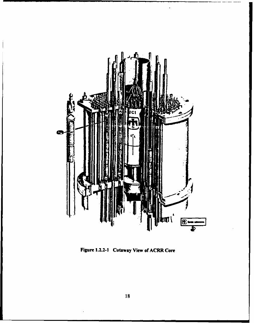
Figure 1.2.2-1 Cutaway View of ACRR Core

18

1.3 Omanization of Report

This report describes the theoretical analysis and simulation evaluation for the

adaptive reactivity model for the enhanced operation of the MIT-SNL neutronic power

controller. Chapter Two defines the methods of reactivity measurement used for

implementation of the neutronic power controller. It also develops the equations used to

implement the reactivity balance model for predicting feedback reactivity from reactor

temperature variations. Chapter Three derives the equations needed to implement the heat

deposition model of the reactor core that was used to generate analytic values of fuel

temperature. Chapter Four develops the estimation routine needed to obtain the reactivity

model adaptation to compensate for modeling errors and the time-varying nature of the

thermal-hydraulic parameters. Equation derivations cover the basic principle of minimum

variance estimation, Kalman estimation, and the extension of Kalman estimation

techniques to non-linear systems. Chapter Five describes the simulations used to verify

the effectiveness of the modeling techniques proposed for use in the adaptive reactivity

model. Chapter Six describes the parity space validation used to estimate the reactivity

from three independent sources. Chapter Seven addresses the FORTRAN program

implementation of the adaptive reactivity model. Chapter Eight covers the final simulation

of the FORTRAN program implementation of the reactivity balance model. Chapter Nine

discusses sensor optimization for the minimum-time control laws. A system analysis is

performed to determine the minimum sensor requirements for performing automatic

system fault detection. Chapter Ten discusses areas of future research that would further

enhance the operation of the adaptive reactivity model. The appendices contain sample

input and output files used for reactivity model simulations.

19

2. Nuclear Reactor Reactivity Model

As described in Chapter One, determination of accurate values of both the thermal

feedback reactivity and the net reactivity is required to implement the MIT-SNL period-

generated minimum time control laws. In addition to these reactivity inputs, it is also

necessary to establish the net rate of change of feedback reactivity. This permits

calculation of the proper control signals for implementing reactor power transients. This

chapter addresses the issues and methods of reactivity measurement used for reactor

power control.

2.1 Dermition of Reactivity

The "effective neutron multiplication factor", Keff, is used to characterize the

state of a nuclear reactor. Keff is the ratio of neutrons produced from fission to those that

are lost through leakage or absorption. Thus, for a critical reactor Keff would have a

value of unity. Reactivity can be defined in terms of Keff. This definition is:

_ Keff -1 (2.1-i)Keff

where p is the reactivity [7]. The reactivity can be thought of as the fractional deviation of

the neutron population in the reactor per neutron generation or lifetime. It should be

noted that both Keff and p are global properties that pertain to the reactor as a whole.

20

Reactivity is dimensionless, and is therefore usually expressed as a percentage.

Reactivity may also be given as a multiple of the effective delayed neutron fraction, Beta.

For example, a reactor with an effective delayed neutron fraction of 0.0073 and a

reactivity of 0.0025 percent, would have reactivity of 0.342 Beta. Another system of

"units" is dollars and cents with one dollar of reactivity being the equivalent of I Beta of

reactivity. In the above example, the reactivity would be referred to as 34.2 cents of

reactivity.

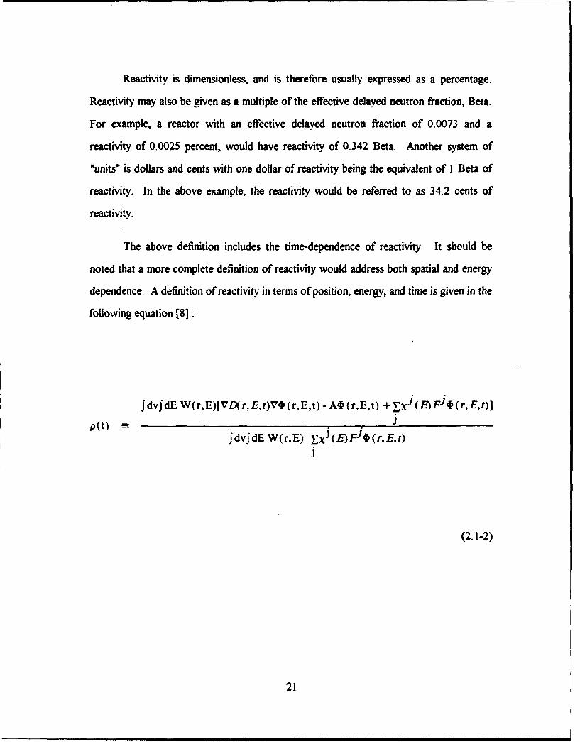
The above definition includes the time-dependence of reactivity. It should be

noted that a more complete definition of reactivity would address both spatial and energy

dependence. A definition of reactivity in terms of position, energy, and time is given in the

following equation [81:

jdvjdE W(r,E)[VD(r,E,t)V4, (r,E,t) - Al (r,E,t) +x ,(E)FAt(r,E,t)]

p(t)JdvJdE W(r,E) y. (E)F4(r,E,t)

(2.1-2)

21

In this equation A and F are integral operators defined through their operation on

any function f (rE,t) with j denoting a particular fissionable isotope. These equations for

the integral operations are [9] :

Af - E, (r,E,t) f(r,E,t) -fE,(r,E'-* E,t) f(r,E',t)dE' (2.1-3)0

Ff f -fv (r,E',t) f(r,E',t)dE' (2.1-4)0

The remaining symbols are defined as:

W(r,E) is the weighing factor for "Neutron Importance",

D(r,E,t) is the diffusion coefficient,

4, (r, E, t) is the neutron flux density,

X(E) is the fission spectrum,

I(r,E,t) is the total macroscopic cross section,

rs(r,E'-.E,t) is the macroscopic scattering cross section, and

E,(r,Et) is the macroscopic fission cross section.

The concept of reactivity as a time-position and energy-dependent quantity is

important when developing methods for reactor reactivity estimation. A given estimation

22

method may assume reactor properties to be constant in energy throughout the core.

While this may not be incorrect for a given set of reactor conditions, it must be recognized

as a limitation of the method employed.

2.2 Assumptions In Reactivity Estimation

Presently two methods of reactivity measurement are widely employed. These are

inverse kinetics and reactivity balances. These are further discussed in section 2.3. The

major assumptions associated with these methods lead to the conclusion that reactivity can

be calculated only as a function of time. The energy dependence in the inverse kinetics

method is eliminated by use of the effective delayed neutron fraction, 3i. This method

allows the energy dependence of the delayed neutrons to be described by the ratio of the

"instantaneous" weighted rate of delayed neutron production divided by the

"instantaneous" weighted rate of all neutron production due to fission [10]. The spatial

dependence in the inverse kinetics method is eliminated through the assumption that the

neutron flux, t, is a product of the flux shape, S, and a flux amplitude function, T. This

relation is given by the following equation:

S(r,E,t) T(t) = ,(r,E,t) (2.2-1)

Thus, if the flux shape is assumed not to change, and appropriate weighting functions are

chosen, the estimation of the flux will be given by the amplitude function which depends

on time alone.

The reactivity balance method also employs energy and spatial assumptions. The

standard procedure is to determine reactivity coefficients through a specific experiment

and/or theoretical calculation and then to apply these coefficients to a variety of reactor

23

conditions. In reality, the coefficients are only accurate for the given reactor flux shape

and the set of conditions present when the coefficient calculation or measurement was

performed. Comparisons of reactivities determined using different methods and

assumptions must be carefully analyzed. Failure to ensure the validity of the underlying

assumptions used in reactivity measurement could lead to an incorrect estimation of

reactivity.

2.3 Reactivity Measurement Methods

The reactivity methods considered here for reactivity estimation and validation are:

"* Inverse Kinetics

"* Reactivity Balances

"* Instrumented Synthesis

2.3.1 Inverse Kinetics

The Inverse Kinetics method of reactivity measurement is based on the space

independent reactor kinetics or "point kinetics equations" [I l. These equations are:

dT(t) _ (t) -13,dt - A T(t) + PACI (t) +Q(t) (2.3.1-1)

24

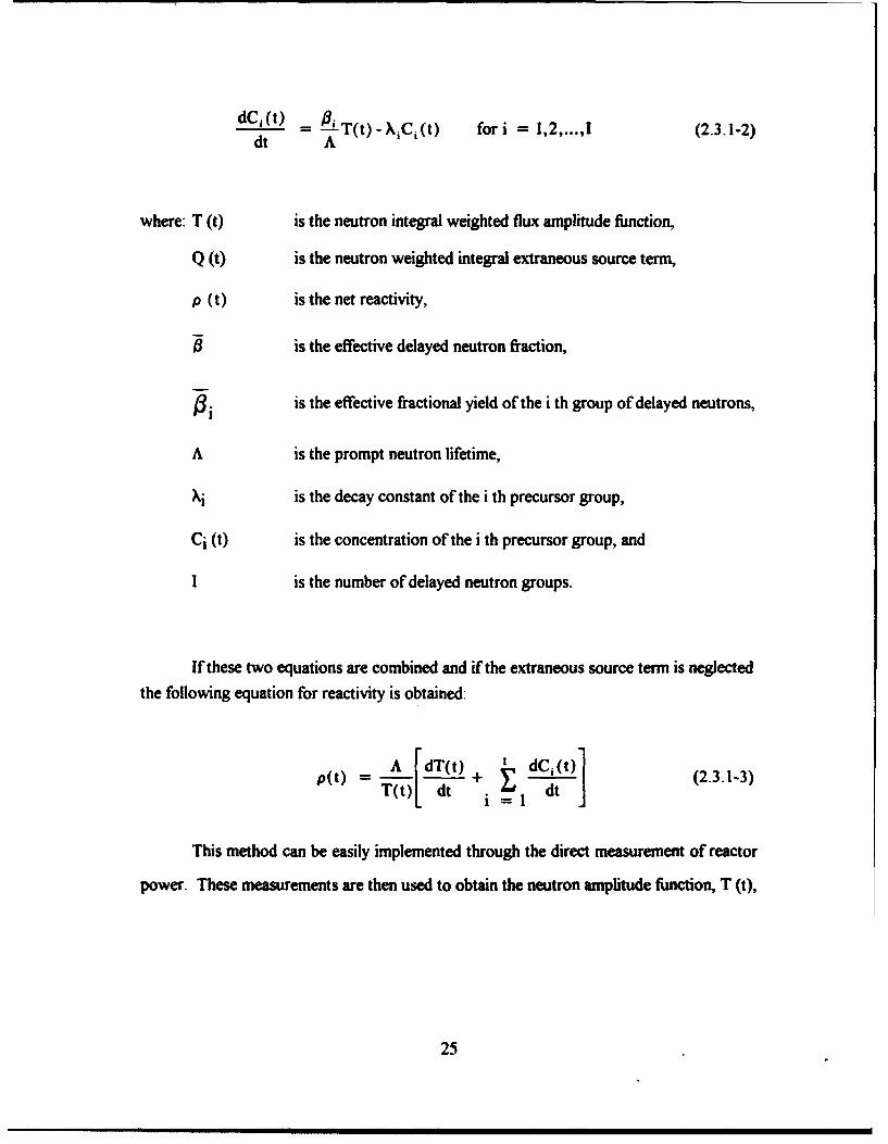
dC -- T(t) - XiCi(t) for i = 1,2,...,1 (2.3.1-2)dt A

where: T (t) is the neutron integral weighted flux amplitude function,

Q (t) is the neutron weighted integral extraneous source term,

p (t) is the net reactivity,

0is the effective delayed neutron fiaction,

(3 is the effective fractional yield of the i th group of delayed neutrons,

A is the prompt neutron lifetime,

Xi is the decay constant of the i th precursor group,

Ci (t) is the concentration of the i th precursor group, and

I is the number of delayed neutron groups.

If these two equations are combined and if the extraneous source term is neglectedthe following equation for reactivity is obtained:

A [dT~) _(t)

P(t) = [dT(t)+i =dC(2.3.1-3)T(t) dt -

This method can be easily implemented through the direct measurement of reactor

power. These measurements are then used to obtain the neutron amplitude function, T (t),

25

which can then be used to estimate the precursor concentrations. The reactivity can then

be determined. This implementation is displayed in Figure 2.3.1-1 [12].

2.3.2 Reactivity Balance Method

The reactivity balance method is easily implemented Normally, it relies on

identification of those reactor parameters that can have an effect on the reactor's effective

neutron multiplication factor, Keff These parameters may include fuel and moderator

temperatures, control rod position, xenon concentration, and others. For each of these

parameters, a reactivity coefficient is determined via experiment or theoretical calculation.

A comparison of each parameter to its initial reference value is then made. This reference

state is usually the condition that exist with the reactor critical at some steady-state power

level. This allows a value of zero for the reactivity reference state.

26

I -

ml �II

'0

U4'2UU,a4'

QU4'

S

U, a - U,

U 0U S

C4' a j ES0

U

fe).

C�4

U

1�

27

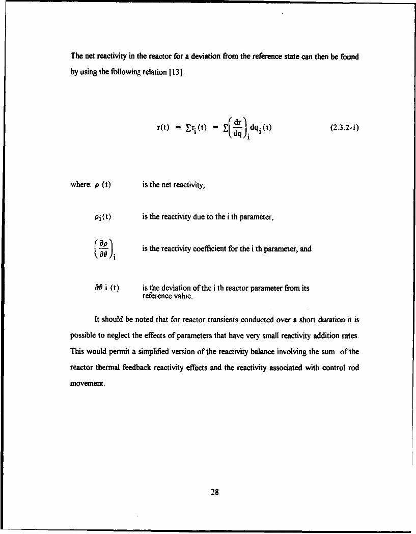
The net reactivity in the reactor for a deviation from the reference state can then be found

by using the following relation [131.

r(t) = J~r.(t) = Ecdr) dq (tM (2.3.2-1)

where: p (t) is the net reactivity,

Pi (t) is the reactivity due to the i th parameter,

(80) is the reactivity coefficient for the i th parameter, and

a0 i (t) is the deviation of the i th reactor parameter from itsreference value.

It should be noted that for reactor transients conducted over a short duration it is

possible to neglect the effects of parameters that have very small reactivity addition rates.

This would permit a simplified version of the reactivity balance involving the sum of the

reactor thermal feedback reactivity effects and the reactivity associated with control rod

movement.

28

This simplified reactivity balance can be implemented using the following relation:

) Prods6 + bfP + mod dp(t) - 6 z 6#f bimod (2.3.2-2)

where: 0 z is the control rod travel from the reference position,

8 f is the change in the average fuel temperature from thereference state,

a # mod is the change in the average moderator temperature from the

reference state,

ap rods is the differential control rod worth at a given position,a z

ap fuela f is the fuel temperature coefficient of reactivity at a given

temperature, and

ap moda rmod is the moderator coefficient of reactivity.

This simplified reactivity measurement method is implemented by determining the

differential rod worth for the controlling rod group and the thermal reactivity coefficients.

The change in rod position, fuel temperature, and moderator temperature can be obtained

either directly from reactor plant instrumentation or via calculations using analytical

reactor models. This implementation is shown in Figure 2.3.2-1.

29

S iSU U S

0

U

0U

A) U5.._ U S-" U �4d

S

U Sto

* S ill *J S0�

� _

5 .� _I *�';�III 000

0.4CE?

SI.U

*UU ..a0 UUI�*4 �U

e;g vJ

30

2.3.3 Instrumented Synthesis Method

A third method for reactivity measurement is presently being investigated. This is

the Instrumented Synthesis Method. This work is being pursued under the direction of

Professor Allen F. Henry, Professor David Lanning, and Dr. John A. Bernard at MIT.

The technique will employ continuous data from distributed in-core detectors to evaluate

local core power distributions thereby allowing the global reactivity to be calculated [1 4].

The basic concept of the method is to estimate the instantaneous local neutron flux

through the use of a linear combination of pre-computed, three-dimensional, static

expansion-functions that bracket an expected reactor transient. The time-dependent

coefficients of these functions are found by requiring the reconstructed neutron flux to

agree with the locally obtained count rates from the in-core neutron detectors. If properly

selected, these expansion-functions will account for variations in flux shape during

transients. This leads to a potentially very accurate prediction of core power distribution

and calculated global reactivity values without the spatial limitations of methods such as

space-independent kinetics. A detailed explanation of this method is given by R. P.

Jacqmin in the 1991 report "Combined Use Of In-Core Neutron Detectors and

Precomputed, Three-Dimensional, Nodal Flux-Shapes Neutron Distribution In Light-

Water Reactors" [15]. An excerpt from this paper is provided in Appendix E.

31

2.4 Chanter Summary

The net reactivity, the rate of change of reactivity, and the precursor distributions

characterize the power response of a nuclear reactor. Values of these parameters are

needed to implement automated reactor control methods. The three methods considered

here for reactivity measurement are Inverse Kinetics, Reactivity Balances, and

Instrumented Synthesis. The use of these three "independent" methods of reactivity

measurements for reactivity signal validation is discussed in Chapter Six. Considered next

are the thermal-hydraulic relations required to implement a reactivity balance model.

32

3. Thermal-Hydraulic Reactor Model

In order to implement a reactivity balance model of a nuclear reactor it is necessary

to develop an analytic method for predicting changes in the temperatures of the reactor

fuel and moderator. This chapter details the theoretical development of an energy

deposition model of a nuclear reactor fuel and moderator.

3.1 Enermy Deposition Model

The basis of the thermal-hydraulic reactor model is a heat deposition model of the

reactor core. These heat balance equations are [161:

Rate of Heat 1 Rate of Energy Rate of

Energy Change = Deposition in the - Heat Energy Loss

[in the Fuel -Fuel From Fission] [To Cooling Media (3.1)

"Rate at"Rate of Rate of Heat "Rate of Heat whith at

which HeatHeat Energy Energy Deposition Energy Transfer Energy isChange for for Moderator within the Con + from Fuel to Carried FromModerator from Fission Moderator The Core

Lwithin the Core (Gamma Heating) within the Core Moderator

(3.1-2)

33

The individual blocks of these equations were developed by Professors Neil E.

Todreas and Mujid S. Kazimi in their text "Nuclear Systems I - Thermal Hydraulic

Fundamentals" [171. They use a lumped parameter integral approach to develop a

simplified set of equations for the fuel and moderator rate of energy change in terms of

material temperatures. These equations use core-averaged parameters for the material

thermodynamic properties as well as core-averaged material temperatures. The use of an

average material temperature assumes a linearly-developed temperature profile within the

material. These individual block relations are:

Rate of HeatEnergy Change =PfuelVfuelC pfueI= ptin the Fuel (3.1-3)

[Rate of Heat 1#modEnergy Change = Pmod Vmod C pmod t

in the Moderatorj (3.1-4)

Rate of Heat 1Energy Deposition|

in the Fuel From

Fission 1

34

Rate of Heat Energy

Deposition from Fission 'YXfuel f 4IVfuel

in the Moderator (-yheating) (3.1-6)

Rate of Heat Transfer

Loss / Gain by ] Afuelh(iffiel - imod)

-Fuel / Moderator (3.1-7)

[ Net Rate of Energy Loss

by Moderator within the = MC (0in . 0 °ut

Core via Moderator Flow- Pmod mod mod (i (3.1-8)

where: p mod is the average moderator density,

P fuel is the average lumped fuel material density,

CPfuel is the average lumped fuel material heat capacity,

C Pfuel is the average moderator heat capacity,

A is the lumped fuel materials surface area,

h is the overall heat transfer coefficient for the fuel material to the

coolant,

y is the percent of thermal energy from fission deposited in the

moderator via gamma heating,

35

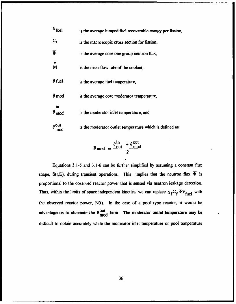
Xfuel is the average lumped fuel recoverable energy per fission,

Ef is the macroscopic cross section for fission,

4)is the average core one group neutron flux,

M is the mass flow rate of the coolant,

Sfuel is the average fuel temperature,

# mod is the average core moderator temperature,

in

#mod is the moderator inlet temperature, and

0out is the moderator outlet temperature which is defined as:mod

0in + 0out

Smod - out mod2

Equations 3.1-5 and 3.1-6 can be further simplified by assuming a constant flux

shape, S(rE), during transient operations. This implies that the neutron flux F is

proportional to the observed reactor power that is sensed via neutron leakage detection.

Thus, within the limits of space independent kinetics, we can replace Xf f VWfuel with

the observed reactor power, N(t). In the case of a pool type reactor, it would be

advantageous to eliminate the mout term. The moderator outlet temperature may bemod

difficult to obtain accurately while the moderator inlet temperature or pool temperature

36

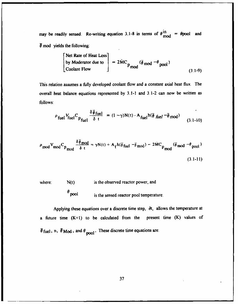
may be readily sensed. Re-writing equation 3.1-8 in terms of a0in = pool and

mod

Smod yields the following:

Net Rate of Heat Loss]

by Moderator due to - 2MC (0mo od - 0 Poo

Coolant Flow Pmod (3.1-9)

This relation assumes a fhlly developed coolant flow and a constant axial heat flux. The

overall heat balance equations represented by 3.1-1 and 3.1-2 can now be written as

follows:

P fuel VfuelCp 5 fuel = (1 -,y)N(t) - Afuelh(# fuel -jrmod)V.,elpfuel 6 t (3.1-10)

S V m p 60mod yN(t) + Afh(ýfuel -ýmod) - 2MC (0mod -pool)rod mod pmod 6 tmod

(3.1-11)

where: N(t) is the observed reactor power, and

0pool is the sensed reactor pool temperature.

Applying these equations over a discrete time step, at, allows the temperature at

a future time (K+I) to be calculated from the present time (K) values of

#fuel, n, #Mod, and 0pool These discrete time equations are:

37

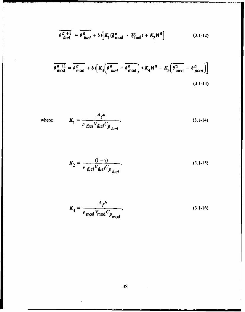
on +1 =-9on + 6 t[Ki(On~ -n )~+KNR31-2

fuel fuel mod (3.1-12)

S= 0(on + at - +K4 Nn Kr9O Omod mod fuel mod mod pool)]

(3.1-13)

Ahwhere: K1 =I (3.1-14)

P fuel VfuJ]Cpfe

/(2 (1 3') ,(3.1-15)

P fuel vfueCpl Sfuel

K A th(3.1-16)P mod 'mod Cmod

38

Kd4 , and (3.1-17)4= mod Vmnod Cmo

Pmod

K- mmod (3.1-)

3.2 Model Limitations

These discrete time equations form a linear system model for fuel and moderator

temperature prediction. This model assumes that the core-averaged lumped thermal

parameters are constant with temperature. This is not an accurate assumption for

transients that cause large temperature changes. For model accuracy, it is necessary to

ensure that the thermal parameters are properly modeled as functions of either moderator

or fuel temperature.

The temperature dependence of the core thermal parameters causes the thermal-

hydraulic model of the reactor to become non-linear. This non-linearity complicates the

estimation of model parameters for use in model adaptation or self alignment. A method

for achieving model adaptation or self alignment is discussed in Chapter Four.

39

The energy deposition model also relies on the previously stated assumptions of

"* Constant flux shape

"* Linearly developed temperature profiles

"* Fully-developed constant flow

"* Constant radial heat flux

Prior to model implementation, for a given reactor design, it is necessary to verify

the accuracy of the model3 integral lumped parameter approach. The comparison of this

energy deposition model to a discrete finite element system model is performed in

Chapter Five.

3.3 Chaipter Summary

In this chapter a generic energy deposition model of a reactor core has been

developed. This model is capable of tracking fuel and moderator temperatures during

reactor operations. The model uses lumped, integral, core-averaged thermal-hydraulic

parameters and assumes a linear, fully-developed, temperature distribution throughout the

fuel and moderator. While generically developed, the final relationship, equations 3.1 -12

and 3.1-13, are specially tailored for the modeling of a pool type reactor. Model inputs

include the initial moderator temperature (0 mod), initial fuel temperature (0 fuel),

reactor power (N), and reactor pool temperature (0 Pool) at discrete time intervals. The

model is linear for constant thermal-hydraulic parameters and provides a suitable basis for

use with model-adaptive or self-aligning routines. However, the temperature dependence

of the thermal-hydraulic parameters in the model required to operate over an extensive

40

temperature range introduces a non-linearity which greatly effects the method of model

adaptation. The following chapter examines a method of adaptive self-alignment for a

non-linear system model.

41

4 Reactivity Model Adaptive Routine and Parameter Estimation

In Chapters Two and Three, models were derived for predicting reactor fuel and

moderator temperatures as well as reactivity. These models were based on energy

deposition relations that use integral, lumped, core-averaged thermal-hydraulic parameters

coupled with a reactivity balance model. These model parameters were a function of the

material's temperature. Values for these parameters are obtained either by theoretical

calculation or through experimentation on the reactor being modeled. During reactor

operation, the actual values of these parameters could vary slightly from those originally

obtained. Should this occur, it would be advantageous to allow the model to adapt to

these parameter changes. This chapter details a method for model adaptation by use of

minimum variance estimation in the form of an extended Kalman Filter.

4.1 Minimum Variance Estimation

We can develop a system estimation scheme in terms of system parameters, X, and

system outputs, Y. Such an analysis is described in "Optimal Filtering" by Brian D.

Anderson and John Moore [ 18]. A possible estimation scheme is shown in Figure 4.1-1.

As an example, we might examine a solution of form Y = AX = alxj + 0 0 0 + anxn

where A is an m x n matrix and X is the state vector. We can define any error inherent in

this system by an error term (e) where e = Y - AX. As an estimator of x we could

choose the criteria to minimize the variance of the square error. (i.e. minx F, ei2 ). This

type of estimation is known as a "Least Square Error" estimation.

42

U .

ETT

<

la-

U

43

The solution [19] to this minimization is easily shown to be:

A T "X = (ATA) -Ay (4.1-1)

This result lends itself to recursive parameters estimation. One such type of method is

Kalman Filtering or Kalman Estimation.

4.2 Kalman Estimation

The Kalman Estimation technique can be applied on a discrete system such as the

following:

Xk+ I = FkXk + GkWk (4.2-1)

Z =HTX +v (4.2-2)

where: k is the discrete time step,

X is the system state,

Z is the system output,

Vk,Wk are the white noise signals, and

Fk,Gk,Hk are the system descriptive matrices.

44

The recursive equations for estimating the system state are derived as follows [20j.

A A AXk/k = Xk/k-I + E/ H ,(HTk Hk Y- (Zk . HTXk/k-i k /-k k/k-i

(4.2-3)

k/qk = Ek/k1- - k/k- I Hk (HT Ek Hk +Rk)-H I kk

(4.2-4)

A 'A

X = [Fk - KkHk Xk•]kx•_ + K Jk

(4.2-5)

iY~ k[IqE 14k I-EIVk -IH kT k Jk- I Hk + Rk) HkTEVk-IrTGkGk

(4.2-6)

Kk = 'klkk- I Hk[H/ lk +k]

(4.2-7)

~k FTF =P -k T k0

(4.2-8)

45

where: E k is the error covariance matrix,

Pk is the state covariance matrix,

Qk is the reciprocal of the state covariance matrix,

Kk is the Kalman gain matrix,

Rk is the noise covariance matrix,

k/k is the solution at time k calculated with k known values,

k+l/k is the solution at time k+l calculated with k known values, and

k/k-I is the solution at time k calculated with k-I known values.

The Kalman estimator can be initialized by selecting E 0/-1 = Po = (FoTFo)"1.

Equations 4.2-3, and 4.2-4 can be viewed as the estimator equations. They determine the

best estimate of the state, x, and the difference or error covariance, 1 k. These estimates

are based on current system parameters and the previously estimated state and covariance

values. Equations 4.2-5 and 4.2-6 are used to propagate the solution forward. This

provides a means of continuously updating a system's state by means of the Kalman

estimator routine. It should be noted that the estimator tends to become "saturated" after

numerous samples. This could lead to a change in the system's state not being detected.

This difficulty can be overcome by periodically reinitializing the Kalman estimator. This

type of estimation arrangement is often termed a state observer because the model's state

46

is estimated based on the difference between the model output and the actual system

output.

For linear systems, this estimation routine, produces an "optimum" estimation or

arrival trajectory to the desired state. The calculations are greatly complicated if the

system of equations under consideration is not linear. To estimate the state of a non-linear

system model it is necessary to extend the Kalman estimator routine to handle the non-

linearity.

4.3 The Extended Kalman Estimator

To use the Kalman estimator for linear systems on a non-linear system model we

must first linearize the system equations. The system equations are now given as:

Xk+l = fk (Xk) + gk (Xk) wk (4.3-1)

Zk = hk ( Xk) + vk (4.3-2)

These system equations are very similar to those of the linear system model given in

equations 4.2-1 and 4.2-2 except that the system matrices are now non-linear functions of

the systems state. To linearize these equations, a first order Taylor Series Expansion is

used [21J.

47

For this method, the following partial derivatives are used:

a fkJ (4.3-3)

HT _ hk (x)(43)k bxIx = lk/k

Gk = gk(k/k) (4.3-5)

Thus, neglecting higher order terms, the new linearized system of equations becomes:

X k +1 = FkXk + Gkwk + Uk (4.3-6)

Zk = HTk k (4.3-7)

48

with Uk and Yk as error signals given by:

Uk = fk('k/k)- Fkikk (4.3-8)

Yk - k('k/k) k H~k/k- 1(.39

Given these linearized system equations, the estimator equations for the Extended

Kalman estimator can be written. These equations are:

* iI (4.3-10)k/k- k/k- I + LkIzk- "k(Xklk - I.-

Xk + Ilk fk(xk/k) (4.3-11)

Lk = E'k I 0 1 k] (4.3-12)

49

a =Hj (4.3-13)

,# k l vk - I El/k - IHkHk lik - IHk tH ik _ I Hk +Rk I- Alk - 1

(4.3-14)

Ek + Ilk = Fk EkFk +k k k k (4.3-15)

The above extended Kalman estimator uses an estimator gain, Lk, calculated in a

manner similar to the standard Kalman estimator gain, Kk. The estimator functions in the

same manner as the standard Kalman estimator with a single exception. Specifically,

because of the system non-linearity, the trajectory to the desired system state can no

longer be guaranteed optimal. Variations of this extended Kalman estimator using the

higher order terms of the taylor series expansion may improve the estimator trajectory at

the cost of using longer, more involved estimation calculations.

50

4.4 Reactivity Model Adaptation Enuation Development

The method of state estimation using an extended Kalman estimator can be applied

to the reactivity balance model developed in Chapters Two and Three to achieve model

adaptation to varying system parameters. The state equation for the reactivity balance

model can be written as follows:

"Tf(k + 1) fk(Tf ,akbkCk)"

fk

a(k + 1) ak

x(k +1) = (4.4-1)

b(k + 1) bk

c(k + l) ck

reactivity = hk (Xk) +vk

The system's state variables are the fuel temperature and the system thermal-

hydraulic parameters appearing in the prediction equation for the fuel tempel..ture. Using

the technique outlined in the previous section, we can write the linearized equations as:

x(k +1) = Fkxk + el (4.4-2)

51

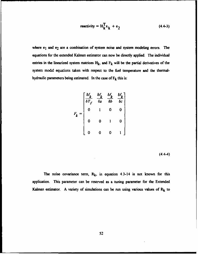
reactivity = HTxk + e2 (4.4-3)

where el and e2 are a combination of system noise and system modeling errors. The

equations for the extended Kalman estimator can now be directly applied. The individual

entries in the linearized system matrices Hk, and Fk will be the partial derivatives of the

system model equations taken with respect to the fuel temperature and the thermal-

hydraulic parameters being estimated. In the case of Fk this is:

6 Tf 6a 6b &c

0 1 0 0Fk

0 0 1 0

0 0 0 1

(4.4-4)

The noise covariance term, Rk, in equation 4.3-14 is not known for this

application. This parameter can be reserved as a tuning parameter for the Extended

Kalman estimator. A variety of simulations can be run using various values of Rk to

52

determine which value allows the adaptive routine to best estimate the system parameters

while still providing robust estimator operation.

4.5 Chapter Summary

A method for achieving model adaptation as a means for providing model error

correction by means of Extended Kalman estimation has been examined. The Extended

Kalman estimation routine provides for linearizing a system model by means of a Taylor

Series Expansion. The linearized model provides a system of equations for state

identification. The system state consists of the Reactivity Balance Model's fuel

temperature as well as specified thermal-hydraulic parameter coefficients that may vary

during reactor operation. The Extended Kalman estimator routine provides a means for

estimating the best values of the system parameters needed to minimize the reactivity error

between the modeled system reactivity and a provided reactivity signal of the reactor

system.

53

5. Verification of the Adaptive Reactor Reactivity Model

An adaptive reactor reactivity balance model can be constructed from the methods

described in Chapters Two, Three, and Four. This chapter examines the construction of

this model for the Annular Core Research Reactor at Sandia National Laboratories in New

Mexico. Verification of the methods of the preceding chapters is accomplished through

simulations using various computer mathematical software.

5.1 Parameter Selection

To employ the equations developed in Chapters Two, Three, and Four, a variety of

reactor thermal-hydraulic and neutronic parameters were required. Many of the rcactor

parameters were obtained from a copy of Chapter Four ( Reactor Design ) of the Annular

Core Research Reactor ( ACRR ) Safety Analysis Report ( SAR ) [221. This copy, which

is currently under revision, was obtained courtesy of Mr. F. Mitch McCrory of the

Reactor Applications Department at Sandia National Laboratories in Albuquerque, New

Mexico. In addition to the SAR reactor design data, various thermal-hydraulic parameters

of reactor materials were obtained from material reference handbooks, such as "The

Metals Reference Handbook" [23], "The Handbook of Applied Thermal Design" [24],

"Thermophysical Properties of Liquids and Gases" [251, and "Nuclear Systems I" [261.

Thermal-Hydraulic parameters that vary with temperature were calculated as polynomial

functions instead of using tabular data. This was done to facilitate the partial derivatives

necessary for implementing model adaptation via the Extended Kalman estimation. The

fuel cell dimensions and core geometry needed for calculations were also obtained from

Chapter Four of the ACRR's SAR.

54

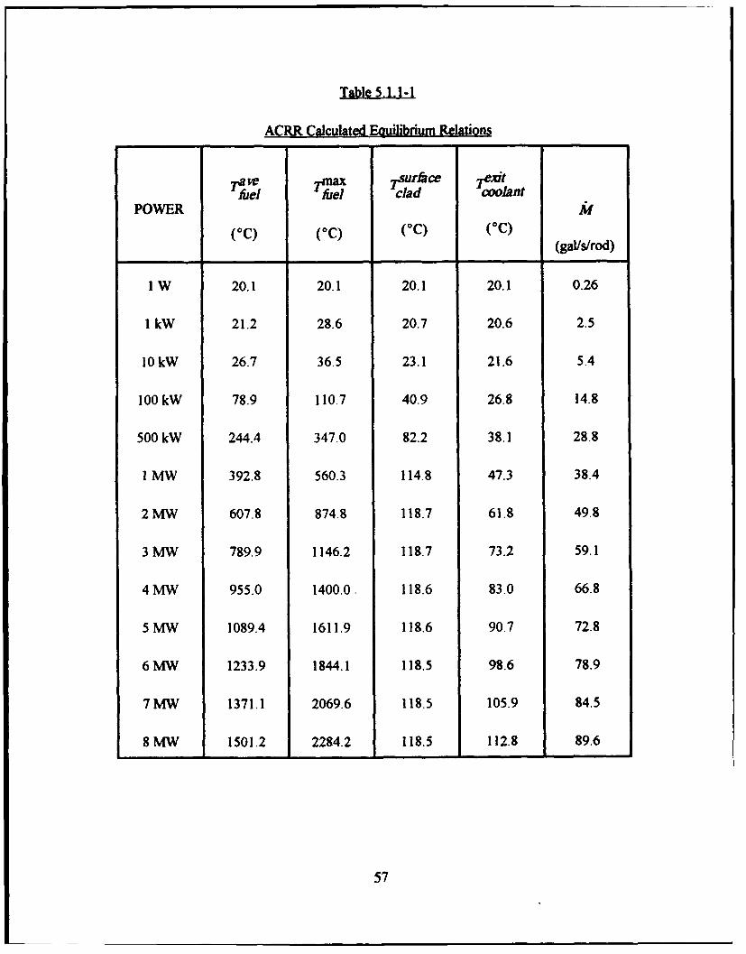
5.1.1 Overall Heat Transfer Coefficient

The overall heat transfer coefficient of the fuel as a function of fuel temperature and the

coolant mass flow rate as a function of moderator temperature were obtained from the reactor

data provided in Chapter Four of the ACRR's SARI Table 4.3-7 of the SAR provided

equilibrium power, temperature, and flow conditions calculated for the ACRR [27]. These

equilibrium conditions were benchmarked to four megawatts via reactor testing. The data

from the SAR is provided here in Table 5.1.1-1. The table data assumes a constant inlet

coolant temperature of 200 C. The overall heat transfer coefficient, h (watts/m2), was

calculated at each equilibrium temperature using the following relation:

h Ph= r 1(5.1.1-1)

7I" 201236 [T"xit+- m 0.59799f 2

where: P is the reactor power (Watts),

Tf ave is the average fuel temperature (0 C),

Tm exit is the moderator exit temperature (Q C),

236 is the number fuel cells in ACRR,

20 is the moderator inlet temperature (0 C), and

55

0.059799 is the heat transfer surface area of a single fuel cell (m2 ).

A polynomial relation between the calculated data points was obtained using

Microsoft Excel, a standard PC software package. This polynomial relationship is given

by the following equation:

h =65.021 + 0.4 4 3 8Tf+ 2.6xlO4Tf2 + 7.6xl0"8Tf3 (5.1.1-2)f f f

5.1.2 Reactivity Feedback Coefficient

Chapter Four of the ACRR's SAR gives individual fuel and moderator reactivity

feedback contribution equations [28]. Additional conversations with Mr. F. Mitch

McCrory at Sandia National Laboratories indicated that an alternate equation had been

calculated that gave a combined thermal feedback reactivity coefficient in terms of average

fuel temperature.

56

ACRR Calculated Equilibrium Relations

ie Tsurface 7 exit

Alfel clad coolantPOWER M

(OC) (0 0) (0c) (OC) (gal/s/rod)

1 W 20.1 20.1 20.1 20.1 0.26

1 kW 21.2 28.6 20.7 20.6 2.5

10 kW 26.7 36.5 23.1 21.6 5.4

100 kW 78.9 110.7 40.9 26.8 14.8

500 kW 244.4 347.0 82.2 38.1 28.8

1 MW 392.8 560.3 114.8 47.3 38.4

2 MW 607.8 874.8 118.7 61.8 49.8

3 MW 789.9 1146.2 118.7 73.2 59.1

4 MW 955.0 1400.0. 118.6 83.0 66.8

5 MW 1089.4 1611.9 118.6 90.7 72.8

6 MW 1233.9 1844.1 118.5 98.6 78.9

7 MW 1371.1 2069.6 118.5 105.9 84.5

8 MW 1501.2 2284.2 118.5 112.8 89.6

57

This relationship had been shown by ACRR tests to provide good results for reactivity

feedback calculations [29]. This equation is:

6P feedback 3.85 730 ]) 10-56#f - 273 +ifJ) 0.0073 (5.1.2-1)

where the reactivity coefficient is in dollars of reactivity per degree centigrade. This

relation is used to determine the thermal feedback reactivity in the Reactivity Balance

Model.

5.2 Thermal-Hydraulic Model Verification

The heat deposition model derived in Chapter Three used core-averaged

parameters to predict the average fuel and moderator temperatures. It was necessary to

determine if the lumped-parameter approach using average temperatures could accurately

model the core for both rapid and slow transients. A comparison of the lumped-parameter

model response to that of a nodal heat transfer code was made. The lumped-parameter

heat deposition model as developed in Chapter Three was simulated using MATHCAD, a

PC based mathematical code. The nodal, finite element modeling was performed using

58

HEATING 5, an Oak Ridge National Laboratory, finite element, heat transfer PC code

[311.

5.2.1 Thermal Model Testinit usini MATHCAD

A simplified version of the heat deposition equation was used to determine the

average fuel temperature at individual time steps. This equation was:

ik+l = "k + Omdh(O f)A+ (1- f)Pk (5.2:1)f f -g (k)f PVCpf(0f)

where: 0 f is the average fluel temperature,

0 mod is the average moderator temperature,

h(Ff) is the overall heat transfer coefficient of the fuel to the

moderator as a function of fuel temperature,

A is the fuel heat transfer surface area,

P is the reactor power,

p is the average lumped fuel density,

V is the average lumped fuel volume,

59

Cpf is the average lumped fuel heat capacity, and

A t is the duration of one time step.

Two types of transients were simulated. The first was a ramp power change from

100 kW to two megawatts over an interval of ten seconds. Fuel temperature was allowed

to rise to new equilibrium conditions over a time of twelve minutes. The moderator

temperature for this transient was simulated using steady-state equilibrium values obtained

from Table 5.1.1-1. The second transient was a rapid power spike. Power was simulated

to rise from one watt to 6400 MW in thirteen milliseconds. Power was then simulated to

return to one watt over thirteen milliseconds. This produced a 6400 MW power spike

with a half power width of approximately thirteen milliseconds. Moderator temperature,

during this rapid power transient, was simulated constant at 200C. Sample MATHCAD

input files as well as fuel temperature plots are provided in Appendix A.

5.2.2 Model Conmarison Using Heating 5

The nodal heat transfer code used for temperature response comparison was

HEATING 5, which is a finite-element code developed by Oak Ridge National

Laboratory. The PC version is capable of simulating 400 separate nodes. It can simulate

various materials and allow heat transfer by convection, conduction, and radiation. The

simulation involved constructing an input file to model an average core fuel cell [301. Fuel

cell geometry was specified using the material, geometry, and dimensions for the ACRR

fuel cells as described in the ACRR's SAR Chapter Four [3 11. The energy deposition in

the fuel cell was peaked radially as described in the ACRR SAR Chapter Four [321. The

first transient simulated was a power ramp from 100 kW to two megawatts over a period

60

of ten seconds. Temperatures were allowed to rise to their new equilibrium values as in

the MATHCAD simulation. The moderator temperature was modeled using the method

described for the MATHCAD simulation. The second transient was a 6400 MW power

spike with a half power pulse width of thirteen milliseconds. The moderator temperature

was simulated as constant at 20 0 C. Sample HEATING 5 input and output files for these

transients are shown in Appendix B.

5.2.3 Discussion of Results

The output files from the HEATING 5 analysis were used to calculate average fuel

temperatures at each data time step. This average temperature response of the fuel is

shown in Figures 5.2.3-1 and 5.2.3-2. These results show very similar responses for the

two models under both types of the examined transients. The maximum deviation

between the two models was 1.77% during the rapid transient and 1.85% during the slow

transient.

The temperature profile across the fuel cell during the rapid transient was also

examined. The Heating 5 fuel temperature profile at various time steps is shown in Figure

5.2.3-3. This profile shows that a linear temperature profile exists even during very rapid

transients. Also, the high degree of isolation between the fuel and cladding provide the

thermal profile necessary to allow the use of an average fuel temperature for heat transfer

calculations.

61

Figure 5.2.3-1 Fuel Temperature Response - SlowTransient

700

600

500

400

Heating5S300 - Mathcad

200

100

0

00 0 0 0 0 0 0 0 0 0 0 0 Q 0(0 ( 0 C4 (00 i

Tim (seconds)

62

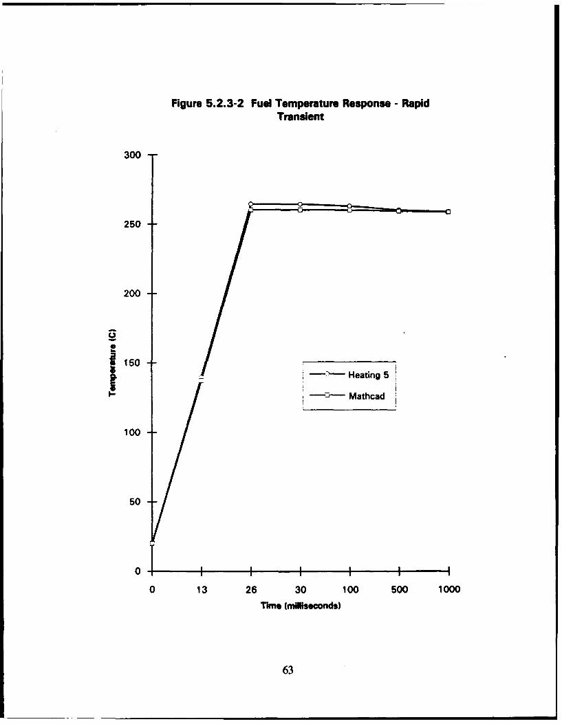
Figure 5.2.3-2 Fuel Temperature Response - RapidTransient

300

250

200

5Heating 5

- Mathcad

100

50

0.1 630 1O 50;0 1000

rime (milliseconds)

63

wv-v, Mop-- , w - IV,-. ----..- ~- ~ - '--.--

Flgure 5.2.3-3 Fuel Temperaturs - RaMdIWOitbution

350-

300-

250 Time=0.O s

- - Time= 0.013 s

~200 - -Time= 0.026 8

-CTime=O0.030 s

r-ime=0.10O s

*10 - 0 - Tire=0.500 s

'Ole- Time= 1.000 s

I Time= 2.000 3

100

50

0~

Ra~dda Position ( m )

64

5.3 Adaptive Estimation Technigue Assessment

Section 5.2 established the proper operation of the heat deposition model for

temperature prediction in the ACRR fuel. The operation of the Kalman Estimation

Technique presented in Chapter Four is examined in this section. The PC-based software

MATLAB was chosen for this assessment because it readily handled the matrix

mathematics required for the Kalman estimation implementation. The simulation involved

a power transient from three kW to four MW over a five second time interval. Power was

then held level at four MW for the duration of the transient.

5.3.1 MATLAB Simulation for ACRR Model

The heat deposition model of Chapter Three was implemented using equations

3.1-12, and 3.1-13. The thermal-hydraulic properties were developed as second order

polynomials to allow for obtaining the partial derivatives required for model linearization.

A data list of input power and associated feedback reactivity was obtained by running the

heat deposition model with an appropriate power signal. Two separate input reactivity

files were generated. The first was the calculated reactivity as generated by the analytic

model. The second file contained the calculated reactivity values with a two percent

random noise signal added. These two files were used to simulate system reactivity inputs

to the adaptive Kalman Estimator routine and there-by to establish the effects of signal

noise on estimator performance. Copies of these MATLAB input files are provided in

Appendix C.

65

The Kalman estimator was implemented using the equations developed in Chapter

Four. Three key thermal-hydraulic parameters were chosen for adaptation. These

parameters were the first-order coefficient of the heat capacity, and the first and second

order terms of the overall heat transfer coefficient. Selection of these specific terms

provides adjustable coefficients for the power, fuel temperature, and the squared fuel

temperature in the heat deposition model. If these model coefficients are set to zero, there

is essentially no heat transfer in or out of the fuel. This allows the Kalman estimator to

derive the best values for the coefficients that "fit" the system's reactivity input signal. To

reduce the effects of system noise on the estimated thermal-hydraulic parameters, a

weighted-average smoothing-function was used. This output smoothing allows the

Kalman estimator to use higher values of gain needed to develop system thermal-

hydraulic parameters rapidly. This smoothed signal could be used to assess the

"steadiness" of the estimated values. The estimation routine employs the following

algorithm:

1. Initialize estimator parameters.

2. Obtain values of system inputs: Power, reactivity, and pool temperature.

3. Obtain current values of model parameters:

"* Reactivity

"* Fuel temperature

"* Moderator temperature

"* Selected thermal-hydraulic coefficients for estimation.

66

4. Calculate the Kalman Estimator Gain.

5. Estimate the "best" values of model reactivity, fuel temperature,

thermal-hydraulic parameters to fit system inputs.

6. Update model with estimated parameters.

7. Repeat steps two through six until the smoothed estimated values of the

model thermal-hydraulic parameters no longer change with each iteration.

Sample MATLAB input files showing this implementation are provided in

Appendix C.

5.3.2 Discussion of MATLAB Simulation Results

The initial simulation run involved input reactivity values with no noise. The

Kalman estimator attempted to derive the best values for reactivity and thermal-hydraulic

parameters based on system input reactivity. The degree of estimator success was judged

by how closely the estimator could determine the original ihermal-hydraulic parameters

used to develop the system input reactivity. A value of 10-15 was chosen for the noise

covariance, R, for the initial run. The sample interval was set at 50 milliseconds. The

MATLAB output charts for this transient are provided in Appendix C. The estimator was

extremely accurate in determining the system thermal-hydraulic parameters. After 50

samples, the estimator had determined the system thermal-hydraulic parameters to within

0.01 percent.

67

A simulation with system input noise set at two percent and R set at 10-!5

produced very poor results. The estimator was not able to determine the system thermal-

hydraulic parameters. This estimator divergence was determined to be the result of an

excessive Kalman gain for the input noise level simulated. To reduce the Kalman gain, the

chosen value of R was set to 10-7.

A simulation with system input noise set at two percent and R set at 10-7

produced a successful estimation run. It was noted that, with the reduced gain, the

estimator took much longer to determine the system thermal-hydraulic parameters than in

the no-noise high-gain run. After approximately 400 samples (20 seconds) the estimator

had determined the system thermal-hydraulic parameters to within 6.18 percent. After

approximately 1300 samples (65 seconds) the estimator had determined system thermal-

hydraulic parameters to within 2.2 percent. Estimator accuracy continued at

approximately two percent through the duration of the simulation. The data generation

scheme was re-run using the estimation values obtained during the simulation. The

generated reactivity using these estimated values fell within the 2% envelope of the

initially calculated reactivity data. The MATLAB output charts for this simulation are

provided in Appendix C.

These simulations show that the estimator routine can accurately determine the

system operating characteristics based solely upon the system input reactivity. The speed

at which the estimator arrives at a stable solution is determined by both the amount of

system input noise and the selected value of the noise covariance. The noise covariance,

R, should be choose to provide the "optimum" solution. Excessively small values of R

68

lead to excessive Kalman estimator gain and divergence of estimated values. Excessively

large values of R lead to longer solution times.

5.4 Chapter Summary

The verification of the adaptive reactor reactivity model was accomplished by

means of simulations using a variety of PC-based heat transfer and m'athematical software.

A comparison of the heat deposition model of the ACRR, simulated in MATHCAD, was

made against a thermal-hydraulic simulation of an average ACRR fuel rod using Heating

5. The simulations showed that the heat deposition model of the ACRR using average

temperatures and integral, lumped, average core thermal-hydraulic parameters could

accurately predict core fuel temperature. Simulation of the adaptive routine using a

Kalman estimator were performed using MATLAB. The estimator determined system

thermal-hydraulic operating characteristics to within two percent of their actual values

when run using a system reactivity signal with two percent noise. Estimator speed for

solution determination was found to be dependent on the input system noise as well as on

the selected estimator gain. Model operation with estimated values of thermal-hydraulic

parameters accurately approximated system operation within the limits of simulated noise.

69

6. Validation of Reactivity Input Sianls

The successful operation of a complex system is dependent upon the validity of the

sensor signals that are use to provide information for control. The use of validated control

inputs serves to enhance controller performance. Validation can be accomplished through

signal averaging which minimizes the effects of signal noise and isolation which eliminates

the effects of faulty sensors. The parity space approach uses redundant sensors to

accomplish fault detection and isolation and thereby provide validated signal inputs for a

control system.

6.1 The Parity Space Approach

The fault detection process can be divided into two stages. These are residual

generation and decision making. The redundant measurements of a process variable can

be modeled by a measurement equation as [33]:

m=-Hx+e (6.1-I)

where m is the (t x 1) vector of measurements that are generated from t sensors, H is

the measurement matrix of dimension (t X n) and rank n, and x is the true value of the

n-dimensional measured variable. The vector z represents measurement errors such that,

for normal functioning of each measurement, the expected value of Ei is zero and

zil( bi, where bi is the specified error bound for the measurement mi.

A measurement of relative consistency between redundant measurements is given

by the projection of the measurement vector m onto the left null space of the measurement

70

matrix H such that the variations in the underlying component Hx in Equation (6.1-1) are

eliminated and only the remaining effects of the error vector e can be observed. An

((e - n) x 0) matrix V is chosen such that its (t - n) rows form an orthonormal basis

for the left null space of H, for example:

VH = 0 vvT = - (6.1-2)

The column space of V is referred to as the "parity space" of H and the projection of m

onto the parity space as the "parity vector," which is represented as:

p = Vm = VE (6.1-3)

The individual parity vector equations are independent of the true values of x and

includes the effects of measurement errors as well as any possible sensor failures [34].

Thus, from Equation (6.1-2), it follows that:

vTv = lf - HIHTHI-IHT (6.1-4)

The column vl, v2 , ... , vt of V, that are projections of the measurement directions (in

Re) onto the parity space are called failure directions because the failure of the ith

measurement mi implies the growth of the parity vector p in Equation (6.1-3) in the

direction of vi. For nominally unfailed operations, the norm IlpIJ of the parity vector

remains small. If a failure occurs, p may (in time) grow in magnitude along the failure

subspace, which is the subspace spanned by the specific column vectors associated with

the failed measurements. If the fault is time-varying, then the failure directions (and hence

the failure subspace) may also be time-varying. The increase in the magnitude of the parity

71

vector signifies abnormality in one or more of the simultaneous redundant measurements,

and its direction can be used for identification of abnormal measurement(s). The parity

vector in Equation (6.1-3) is related to the familiar residual vector n by:

n = VTp (6.1-5)

where n = m - Hi and £ = [HTHV-IHTm, the least-squares estimate of x. From

Equation (6.1-2) it follows that the residual vector and parity vector have identical norms,

for example:

nTn = pTp (6.1-6)

For the application reported here, only scalar measurements were used. Hence, the

dimension of the measured variable x in Equation (6.1-1) is unity. The residual vector can

therefore be written as:

n =VTp

where: (6.1-7)1

ni mi - mj i = 1,2...,f

The residual ni is thus the difference between the ith measurement and the average of all

the redundant measurements.

72

It can also be shown [35] that the individual parity equations can be described as

functions of the signal residuals. This relation is:

Pij2 F n2- ~n2 (6.1-8)

For normal operation, with no failed sensors, the parity vector tends to be small

and the individual Pi are also small. For a set of t measurements it can be shown [36]

that f measurements are mutually consistent (fault free) if the following inequality is

satisfied:

Sb 2 fo r ev en f

Ip 12 < I

f2 Jb2 for odd f

(6.1-9)

Thus, if a failure occurs, the set of t measurements would exhibit inconsistency and the

parity vector would grow in magnitude, exceeding the limiting condition 9e defined by the

error bound b.

73

6.2 Validation Aaonbm Deveonment

The parity space approach of section 6.1 can be used to develop an algorithm for

fault detection and isolation. The algorithm employs the parity vector, p, as a means of

identifying a set of inconsistent or failed measurements. The measurement with the largest

residual, within a failed set, can be discarded and the remaining measurements checked for

consistency. This process leads to the identification of the largest possible set of

consistent measurements. These measurements can be to provide the validated average

signal output. The calculational sequence for validation of ti'ree assumed independent

reactivity measurements with common error bound, b, is given by the following:

1. Calculate the residuals, ni, and the respective parity vectors, pi, for the three

measured reactivity signals.

2. Compute the consistency threshold using the bound b and f equal to three.

3. Test for measurement consistency. If all the pi are less than the consistency

threshold level, set the validated signal to the average of the three input signals. If

one or more of the pi is greater than the consistency threshold level, the

measurement with the largest residual ni is discarded as a faulty reading.

4. Recalculate the residuals, ni, and the respective parity vectors, pi, for the remaining

two reactivity measurements.

5. Compute the new consistency threshold again using b but with t equal to two.

74

6. Test for measurement consistency. If the two pi'S are less than the consistency

threshold level, set the validated signal to the average of the remaining two signals.

If a pi is greater than the consistency level then all three signals are inconsistent

and the validated reactivity signal is set to a default value equal to the inverse

kinetics reactivity signal.

A limitation of this method is that of a "common mode" failure. Common mode failure

implies that two of the measurements fail identically. In this instance the validation routine

would interpret this condition as a failure of the remaining good signal instead of the

failure of two faulty signals.

This algorithm was successfully demonstrated on the MITR-I1 research reactor in

1983 [37]. The algorithm correctly identified and isolated faulty sensor readings resulting

from faulty sensor calibration, gradual drift, increased sensor noise, and total sensor

failure. [note: All of these failures were induced as part of an approved experimental

procedure.]

6.3 Chapter Summary

The parity method for fault detection and isolation can be easily implemented using

the derived relationship of the parity vector to the individual signal residuals. An error

bound, b, specified for the measurements is used to define a maximum bound for parity

comparison. Faulty signals are indicated when the parity vector for a set of measurements

exceeds the calculated consistency threshold. The signal with the largest individual

measurement residual is then discarded. The validated signal set can then be averaged to

obtain a validated signal which can enhance controller performance.

75

7. Control Software Imnlem&ntation

The concept developed in the preceding chapters was written as FORTRAN code

so as to provide the block functions shown in the Reactor Neutronic Power Controller

Block Diagram, Figure 1.2.1-1. It was desired that the code be capable of running input

transient data files available from previous tests conducted on the ACRR. It was also

intended that the code be incorporated as a subroutine of the MIT-SNL Period-Generated,

Minimum-Time Control Law Code [38]. The software was written in FORTRAN 77.

7.1 Subroutine Description

The developed FORTRAN code consisted of a program main body, six

subroutines, and three functions. For model simulation, the main body is capable of

reading input data files simulate reactor operation. The calculation steps included in the

main body can easily be that incorporated into the MIT-SNL Control Law Code,

subroutine "CONPER" [39], to achieve the power controller configuration of Figure

1.2.1-1. The FORTRAN Code, as well as a sample input file, are provided in Appendix

D. The purpose of each of the FORTRAN Code Blocks is summarized here.

7.1.1 Program Main Body

This is the controlling routine for the program. It initializes the system model

parameters to start a specific power transient. The logical parameter "ALIGN" determines

whether or not a predetermined set of thermal parameter coefficients is used in the thermal

hydraulic model for predicting reactor fuel temperatures throughout the transient. If set to

"TRUE", thermal coefficients are reestimated at each time step by the Kalman estimation

76

routine. Otherwise the coefficients are not updated. After parameter initialization, the

following sequence is followed:

1. Validate the three assumed independent reactivity signals to determine the best

estimate of net reactivity as given by variable DKest. Instrumented Synthesis

Method reactivity values were not available. Therefore, an average of the current

step's and previous step's Inverse Kinetics reactivity was used as a third input

signal.

2. Print the desired step output parameters. These could consist of the current time,

the individual reactivity signals, the fuel temperature, and the individual estimated

thermal parameter coefficients.

3. If variable "ALIGN" is "TRUE", a best estimate of the thermal model parameter

coefficients is made and the model is updated to use these values. If variable

"ALIGN" is "FALSE", the model parameter coefficients remain unchanged

throughout the transient.

4. The Thermal Model of the reactor is advanced to the next time-step. This

provides future values of the thermal feedback reactivity and fuel temperature for

controller use.

5. At a specified time, the routine reads the next set of data. This data consists of the

current-time, the reactor power, the Inverse Kinetics reactivity, and the position of

the reactor's transient rod bank.

6. The net reactivity is calculated for this new data via a balance equation.

77

7. The routine continues by repeating step's one through six until all data in the input

file has been processed.

7.1.2 Subroutine Advmodel

The next time step values of the fuel temperature and moderator temperature are

calculated using the thermal model equations. The system matrix values of F, H, and E

are also advanced using the Kalman Estimation prediction equations.

7.1.3 Subroutine Estmodel

A best estimate of the fuel temperature and the thermal reactor model's parameter

coefficients is made via Kalman estimation. This routine is called if the parameter

"ALIGN" is "TRUE".

7.1.4 Matrix Math Routines

The Kalman estimation routine uses matrix equations to determine parameter

estimates. FORTRAN 77 has no intrinsic matrix functions to accomplish basic matrix

mathematics. It was necessary to write basic routines to carry out the operations of

matrix addition, transposition, scalar multiplication, and vector multiplication. These

matrix mathematics routines were provided by Addmat, Transmat, Multscale, and

MatMult respectively. It should be noted that FORTRAN 90 does possess these

mathematical operations as intrinsic functions. Should the control scheme be updated to

use FORTRAN 90, these four subroutines would be unnecessary.

78

7.1.5 Functions Reactr (n) and Reactfb (T.Tin)

Function reactr (p) returns the reactivity associated with a given position of the

reactor's transient rod bank. This function is called by the main body of the program to

determine control rod reactivity for the reactivity balance. Function Reactfb (T,Tin)

determines the feedback reactivity associated with increases in the reactor fuel

temperature. The reactivity coefficient is as described by Equation 5.1.2-1.

7.1.6 Function Validat

Function Validate returns the values of reactivity resulting from .the

implementation of the validation algorithm on the three input reactivity signals. Value b

specifies the common error bound for reactivity signal validation.

7.2 Chanter Summary

The FORTRAN implementation of the Adaptive Reactor Reactivity Model was

developed in FORTRAN 77 and is capable of running input files consisting of current

transient-time, reactor power, Inverse Kinetics Reactivity, and transient rod bank position.

It determines the resulting reactor fuel temperature and net reactivity via a reactivity

balance. The program is capable of estimating model thermal parameter coefficients

which are assumed to be constant during transients. The program can also be executed to

run using predetermined model parameters.

79

S. FORTRAN Software Evaluation

The FORTRAN Code developed in Chapter Seven and provided in Appendix D

was tested using input data obtained from previous MIT-SNL neutronic power controller

tests. These simulations were used to assess the performance of the FORTRAN routines

described in Chapter Seven and to show their capacity to support enhanced operation of

the MIT-SNL Neutronic Power Control Method. The results of these simulations are

summarized here.

8.1 Input File Selection

The input data for FORTRAN Code evaluation was selected from the output data

obtained during a series of experimental evaluations that were conducted on the MIT-SNL

Period-Generated, Minimum-Time Control Law Code in July 1991. The transient selected

was a power increase from three kW to four MW on a 0.695 second period. Reactor

power was then held constant for twenty-five seconds. The data available for the transient

was provided at 0.045 second intervals over the duration of the transient. The data

included reactor power (kW), the calculated inverse kinetics reactivity (millibeta), and the

position of the transient rod bank (units). A copy of this data file is provided in Appendix

D.

8.2 Parameter Estimation Simulation

As a first test of the FORTRAN Code, the transient was run with initial model

thermal parameter coefficients of ao, bo, and bi set to zero; the logical parameter,

"ALIGN", was set to "TRUE"; and the bound for validation was set to two percent.

80

Parameter initialization was conducted using derived values obtained as detailed in Section

5. 1. During this run, the time required for the calculation was also checked to verify that

the individual step calculations could be carried out in real-time for controller operation.

The thirty second data run required approximately 4.5 seconds to execute. This indicates

a single step series calculation time of, on average, 6.75 milliseconds. This meets the

sample time criteria for controller operation [40]. The output data was collected at each

time step and included reactivity via balance calculation, the validated reactivity, the

reactor fuel temperature, and the values of the estimated thermal parameter coefficients

(ao, bo, bl). This output file is provided in Appendix D. A comparative plot of the

various reactivity signals is shown in Figure 8.2-1. This plot shows oscillations taking

place as the estimation routine attempted to determine the best values of reactivity and the

thermal parameter coefficient (ao, bo, b1) . The oscillation magnitude decreased as the

transient progressed. The thermal parameter coefficient values are shown in Figure 8.2-2.

Again, the fluctuations in the parameter value are initially large but, decrease as the

transient progresses. It is noted that in the two percent input noise simulations of the

Kalman estimation routine performed in MATLAB and presented in Section 5.3.1,

estimation variations required approximately forty to sixty seconds to decay away. If an

additional ten to thirty seconds of data had been available a more precise solution might

have been obtainable.

A close examination of the reactivity outputs revealed the proper operation of the

validation routine. When all three values were within the required bounds, as calculated

using b, a three signal estimate was provided for the variable DKest. During oscillations

81

of the balance reactivity, caused by parameter estimation, the routine isolated the balance

reactivity signal and provided a two signal estimate for the variable DKest.

As a final evaluation of the routine's ability to converge to a correct solution, the

FORTRAN Code was run a second time with the thermal parameter coefficients initialized

to the final values obtained during the first estimation run. The logical parameter

"ALIGN" was set to "FALSE" so the simulated transient could be modeled using the

previously determined thermal parameters. The output reactivity values from this

simulation are shown in Figure 8.2-3. The modeled balanced reactivity differs from the

actual inverse kinetics reactivity by approximately ten percent. It is possible that if a more

precise set of thermal parameter coefficients could have been obtained the model's

performance would have provided a more accurate approximation to the reactivity

response. A longer simulation providing more accurate coefficient values could lead to a

better fit of modeled reactor conditions to the actual inverse kinetics values. It should also

be noted, however, that the estimation routine relies on the accuracy of the fuel

temperature reactivity coefficient relationship given in equation 5.1.2-1. Errors in this

relation could also cause the observed differences between the calculated balance

reactivity and the actual inverse kinetics reactivity. It should also be noted that no attempt

is made to verify the accuracy of the control rod reactivity obtained by the Function

Reactr (p). A temperature dependence of transient bank rod worth could also lead to a

modeling error. These possibilities would require additional investigation.

82

CL

C00

UU

c-

o 6ot

2C

Ineq A*b'*O I

(~83

ULCP

ao

a.o

0v

8q 8 8

aaiNW

E8

E

A-A

C69

o) co N 02

Uos) AjL30

85S

8.3 Cbfter Summary

The FORTRAN Code implementation of the thermal-hydraulic reactor reactivity

balance model was run using input data from previously conducted MIT-SNL period-

generated, minimum-time control law code testing on the ACRR. These simulations

showed the ability of the reactivity balance model using the Kalman estimation of model

thermal parameter coefficients, to converge to an actual dynamic reactivity solution.

Convergence after thirty seconds of estimation was to within approximately 100/a of the

assumed actual system reactivity. Additional investigation is indicated to determine if

longer simulation runs would provide more accurate model solutions. Investigation of

other sources of modeling error which are currently not estimated may also be warranted.

86

9. Sensor Ogtimization for Automatic Fault Detection

Chapter Six described the parity space method of fault detection and isolation that

is used to provide signal validation for the assumed independent reactivity signals. It

would be desirable to implement the closed form of the MIT-SNL period-generated,

minimum-time control law code to provide on-line fault detection and isolation. To

achieve this requires an examination of both the inputs available to the control system as

well as the method to be used to achieve fault diagnostics.

9.1 Method of Fault Detection

Methods other than the parity space approach can be used to provide on-line fault

detection for improved system performance. Some of these methods include failure

sensitive filters, statistical innovations, and sequential hypothesis testing [41]. Often the

method selected is based on the desired response of the detection system that is to be

employed. In general, there are usually two conflicting considerations. These are the

speed at which a system responds to a fault and the degree of degradation needed to allow

a fault to be detected. Systems which require a high degree of reliability such as aircraft

or nuclear control systems demand input redundancy to ensure rapid fault detection with a

minimum impact of false alarms. It was this consideration which lead to the use of the

parity space approach outlined in Chapter Six. To implement the parity space approach, a

minimum configuration of redundant sensors must be available.

87

9.2 Minimum Sensor Emnlovment for Fauk Detection

The MIT-SNL Period-Generated, Mimimum-Time Control Law Code relies on

inputs from reactor power, net reactivity, the rate of thermal feedback reactivity, and rod

position and speed to provide the proper rod control signal. The power signals from the

nuclear instrumentation are instrumental in providing input for reactivity calculations as

well as in determining the deviation of the reactor from the desired power level. It is

necessary that a continuous uninterrupted power signal be available across the range of

operation. Most nuclear instruments cover a range of approximately four decades of

power. To achieve adequate sensitivity and accuracy to power level changes across a

wide range of power levels (as many as ten decades of power) a combination of

instruments is used. These nuclear instruments are usually divided into source,

intermediate, and power ranges. A relationship can easily be derived to generate a single,

continuos neutronic power level signal from these three detector ranges [42].

Furthermore, the ranges are designed so that overlap exists from one range to another.

Thus, for operation in the intermediate range, power signal validation could be conducted

using source or power range instruments that exhibit overlap. It should be noted that for

operation high in the power range or low in the source range, signal validation would

require an additional sensor. This sensor could either be a direct neutronic power signal

or an indirect signal derived from an analytic model. As an example, reactor power could

be predicted using the known reactivity and the space independent kinetics equations [43].

Use of an analytic model in place of a direct signal input eliminates the need to provide

additional sensors for the sole purpose of signal validation. Thus, for nuclear

instrumentation, a minimum implementation for fault detection over the entire range of

88

operation could consist of two independent channels of source, intermediate, and power

range with an analytic model capable of predicting the neutronic power level using a

validated reactivity input. These validated power signals along with the validated

reactivity inputs would offer a minimum sensor implementation for on-line detection for

the MIT-SNL period-generated, minimum-time control law.

9.3 Chapter Summary

The parity space approach of signal validation for systems with redundant

measurements provides a rapid means of sensor fault detection and isolation. The MIT-

SNL neutronic power controller requires both validation of net reactivity and reactor

power input signals to provide enhanced system performance. This implementation would

require a minimum of two sets of power, intermediate and source range nuclear instrument

channels along with an analytic model for reactor power prediction.

89

10. Summary. Conclusions, and Recommendations for Future Research

10.1 Summary

This report summarized the development and demonstration of an improved

reactor analytic model for the prediction of thermal feedback reactivity. The output of this

model was used in a reactivity balance to produce a net reactivity signal. This signal was

employed along with two additional, assumed independent, net reactivity estimation

methods in a parity-space fault detection algorithm to give a validated net reactivity. The

end use of this validated net reactivity signal is to provide enhanced operation of the MIT-

SNL period-generated, minimum-time, neutronic power controller. The analytic heat

deposition model for prediction of thermal feedback reactivity included a Kalman state

estimation routine to provide real-time model adaptation to compensate for modeling

errors or parameter drift. The concepts used in the adaptive analytic reactivity balance

model were verified using the PC-based math software MATLAB and MATHCAD, as

well as, a finite difference, heat transfer code, HEATING 5. An adaptive analytic

reactivity model of the ACRR was implemented in FORTRAN 77. A simulation of this

model implementation was conducted. Simulation input was provided from previous tests

of the MIT-SNL period-generated, minimum-time, neutronic power controller on the

ACRR conducted in July 1991.

90

10.2 Conclusions

The lumped average core parameter, heat deposition model of the ACRR, modeled

using MATHCAD, was compared to a nodal, finite difference, heat transfer model of the

ACRR, modeled using HEATING 5. The lumped parameter, average core value model

predicted average core fuel temperatures to within approximately two percent of the

values obtained using the nodal finite difference method. This verification was shown for

both slow and rapid power transients.

The Kalman estimation routine employed to provide thermal model adaptation was

simulated using MATLAB. The simulation verified the ability of the Kalman state

estimation routine to determine analytic model thermal parameters for the purpose of on-

line, real-time model error correction. The simulations used input power and system

thermal feedback reactivity signals, sampled every 50 milliseconds, and corrupted with

two percent white noise. The estimation routine determined the system thermal parameter

coefficients in approximately sixty-five seconds. These estimated parameter coefficients

when used in the analytic reactivity model, produced thermal feedback reactivities that

were within the two percent noise band of the input feedback reactivity.

The final system simulation of the adaptive analytic reactivity balance model and

the reactivity validation routine confirmed the ability of the validation routine to reject

faulty reactivity input signals. The adaptive analytic reactivity balance model determined

best estimates of the model's thermal parameter coefficients during a 30 second simulation.

This simulation used input data obtained from previous MIT-SNL period-generated,

minimum-time, neutronic power controller tests. The length of time required by the

91

routine to carry out the calculations necessary for a single time step was on average 6.75

milliseconds. This met the sample time criteria for controller operation. The estimated

thermal parameter coefficients were in turn used to produce a reactivity balance model

that was capable of predicting system reactivity to within approximately ten percent of the

actual system values. More accurate model thermal parameter coefficients could be

obtained if the estimation were performed for approximately sixth-five seconds of input

data.

10.3 Recommendations for Future Research

The following recommendations involve areas associated with this report that

warrant further research:

1. Additional simulations of the adaptive estimation routine to determine an optimum

set of Kalman estimation parameters that produce the most efficient and robust

response. Parameters affecting estimation routine response include, the noise

covariance matrix (R) and the initial value of the error covariance matrix (E).

Limiting the allowed magnitude of the estimated thermal parameter coefficients

could also be considered to enhance routine response.

2. Additional simulations of the adaptive estimation routine using real ACRR data

over longer transient intervals. Simulations should address determination of a

minimum time required for the estimation routine to determine the model's thermal

parameter coefficients that are capable of predicting future reactivity transients to

within two percent of the inverse kinetics reactivity values.

92

3. Incorporation of the Adaptive Reactivity Model FORTRAN Code implementation

into the MIT-SNL Period-Generated, Minimum-Time, control code. The

combined code could be demonstrated on the ACRR to determine the benefits of

this reactivity estimation and validation scheme on controller performance.

93

References

1. Bernard, J. A., Formulation and Experirental Evaluation of Closed-Form Control

Laws for the Rapid Maneuvering of Reactor Neutronic Power, MIT Nuclear

Reactor Laboratory Report Number MITNRL-030, Cambridge, MA, 1989, p 133.

2. Bernard, J.A., Startup and Control of Nuclear Reactors Characterized by Space

Independent Kinetics, MIT Nuclear Reactor Laboratory Report Number MITNRL-

039, Cambridge, MA, 1990, p 186.

3. Ray, A. and R. Luck (1991) "An Introduction to Sensor Signal Validatiorr in

Redundant Measurement Systems", IEEE Control Systems Magazine, 11(2) : pp

43-49.

4. Bernard, J.A. and D.D. Lanning, "Considerations in Design and Implementation of

Control Laws for the Digital Operation of Research Reactors", Nuclear Science and

Engineering, Vol. 110, Nov. 4, Apr. 1992, pp 425-444.

5. Bernard, J.A., "Non-Linear Control of Neutronic Power in Reactors Described by

Space-Independent Kinetics", International Journal Control-Theory and Advanced

Technology (C-TAT), Vol. 8, No. 3, Sept. 1992, pp 495-511.

6. Lau, S.H., J.A. Bernard and D.D. Lanning (1991). "Experimental evaluation of

feedforward control for the trajectory tracking of power in nuclear reactors". Proc.

26th Inter-society Energy Conversion Engineering Conference (IECEC). August,

Boston, MA, 5, 13-19).

94

7. Henry, A. F., Nuclear Reactor Analysis, MIT Press, Cambridge, MA. 1975, p 78.

8. Ibid. p 304.

9. Ibid. p 299.

10. Ibid. p 305.

11. Ibid. p 302.

12. Sastre, C. A., "The Measurement of Reactivity", Nuclear Science and Engimeering•

Vol. 8, pp. 443-447, Nov 1960.

13. Ibid. p 113.

14. Henry, A. F., Lanning, D.D., and Bernard, J.A., "Experimental Evaluation of an

Instrumental Synthesis Method for the Real-Time Estimation of Reactivity",

Proposal Submitted to the U.S. Department of Energy.

15. Jacqmin, R. P., "Combined Use of In-Core Neutron Detectors and Precomputed.

Three-Dimensional. Nodal Flux-Shapes for the On-line Determination of the

Neutron Distribution in Light-Water Reactors", MIT, Cambridge, MA, 1991, pp 2-

5.

16. Avallone, E.A. and Baumeister, T., "Mark's Standard Handbook for Mechanical

Engineers", McGraw-Hill Book Company, New York, NY, 1987, p 4-5.

17. Todress, N. E. and Kazimi, M. S., "Nuclear Systems - I", Hemispere Publishing

Company, New York, NY, 1990, p 84.

95

18. Anderson, B. D. and Moore, J. B., Optimal Fltering, Prentice-Hall, Inc.,

Englewood Cliffs, NJ, 1979, p 29.

19. Verghese, G., Dynamic Systems, MIT course number 6.241, Classnotes, ( Fall

1992).

20. Anderson, B. D. and Moore, J. B., Optimal Filteing, Prentice-Hall, Inc.,

Englewood Cliffs, NJ, 1979, p 39.

21. Ibid. p 195:

22. Sandia National Laboratories (SNL) Annular Core Research Reactor (ACRR)

Safety Analysis Report, Chapter Four, (Draft Copy - currently under review)

23. American Society for Metals, "Metals Handbook: Vol 2: Properties and Selection:

Non-Ferrous Alloys and Pure Metals", American Society for metals, Metals Park,

Ohio, pp 777-778.

24. Guyer, E. C., "Handbook of Applied Thermal Design", McGran-Hill Book

Company, New York, NY, 1989, p 5-31.

25. Vargafiif, N. B., "Thermophysical Properties of Liquids and Gases", Hemispere

Publishing Corporation, Washington, D.C., 1975.

26. Todress, N. E. and Kazimi, M. S., "Nuclear Systems - I", Hemispere Publishing

Company, New York, NY, 1990, p 84.

96


Safety Analysis Report, Chapter Four, (Draft Copy - currently under review) p 4-57.

28. Ibid. p 4-53.

29. McCrory, F., Sandia National Laboratories, Reactor Applications Department,

personnel communication by phone, (July1992).



31. Turner, W. D. and M. Siman-Tov, "Heating 5 -- An IBM 360 Heat Conduction

Program", Oak Ridge National Laboratory, Oak RidgeTennesseFebruary 1971.



33. Polenta, H. P., Ray, A. and J. A. Bernard, "Fault Detection System For Argentine

Reasearch Reactor Instrumentation", American Institute of Physics CONF 930103,

1993.

34. Ray, A., Desai, M.N., and J. Dejst, "Fault Detection and Isolation in a Nuclear

Reactor", Journal of Energy, Vol. 7, No. 1, Jan. - Feb. 1983, p 81.

35. Ibid. p 82.

36. Ibid. p 82.

37. Ibid. p 79.

97

38. Bernard, J. A., Formulation and Experimental Evaluation of Closed-Form Control

Laws for the Rapid Maneuvering of Reactor Neutronic Power. MIT Nuclear

Reactor Laboratory Report Number MITNRL-030, Cambridge, MA, 1989.

39. Ibid. p 145.

40. Ibid. p 136.

41. Willsky, A. S., "A Survey of Design Methods for Failure Detection in Dynamic

Systems", Automatica, Vol. 12, Nov. 1976, pp 601-611.

42. Bernard, J. A., Formulation and Experimental Evaluation of Closed-Form Control

Laws for the Rapid Maneuvering of Reactor Neutronic Power, MIT Nuclear

Reactor Laboratory Report Number MITNRL-030, Cambridge, MA, 1989 p 149.

43. Ibid. p 42.

44. Jacqmin, R. P., "Combined Use of In-Core Neutron Detectors and Precomputed.

Three-Dimensional, Nodal Flux-Shapes for the On-line Determination of the

Neutron Distribution in Light-Water Reactors", MIT, Cambridge, MA, 1991, pp 2-

5.

45. Kaplian S., 0. J. Marlowe, and J. A. Bewick, "Application of Synthesis Techniques

to Problems Involving Time-Dependence", Nuclear Science and Engineering. 18,

163 (1964).

46. Yasinski J. B. and A. F. Henry, "Some Numerical Experiments Concerning Space-

Time Reactor Kinetics Behavior", Nuclear Science and Engineering. 22, 171 (1965).

98

47. Henry A. F., Nuclear-Reactor Analysis, MIT Press, Cambridge, MA (1975).

48. Stacey W. M., Jr., Space-Time Nuclear Reactor Kinetics Academic Press, New

York, NY (1969).

49. Ryals H. W., "Approximation of Nuclear Flux Distributions in Operating Power

Reactors", Transactions of the American Nuclear Society 4, 750 (1971).

50. Levine M. M. and D. J. Diamond, "Reactor Power Distribution From Analysis of In-

Core Detector Readings", Nuclear Science and Engineering, 47, 415 (1972).

51. Kugler G., "Commissioning and Early Operating of the Bruce A Flux-Mapping

System", Proceedings of IAEA International Symposium on Nuclear Power Plant

Control and Instrumentation, IAEA-SM-226/101. Volume I, 463, Cannes, France

(1978).

52. Knob P. J., R. D. Neef, and H. Schaal, "Development and test of the Three-

Dimensional Computer Code ZELT-3D for Unfolding Power Distributions Using

Side Reflector Instrumentation Signals", Nuclear Technology. 64. 3, 217 (1984).

53. Bonalumi R. A. and N. P. Kherani, "Rational Mapping (RAM) if In-Core Data",

Nuclear Science and Engineering. 90, 47 (1985).

54. Hotte G. A. Baudouin, G. Parent, and C. Ngo-Trong, "Gentilly Core Management

Based on Diffusion Theory and On-Line Monitoring (SIMEX)", Proceedings of the

Topical Meeting on Advances in Fuel Management, Pinehurst, NC (1986).

99

Appendix A

Mathcad Sample Input/Output File - 10 sec power ramp_ 101

Mathcad Sample Input/Output File - 26 millisecond power spike 103

Mathcad / Heating 5 Comparison Data 105

Mathcad Plot of Heating 5 Pin Temperature Profile 108

100

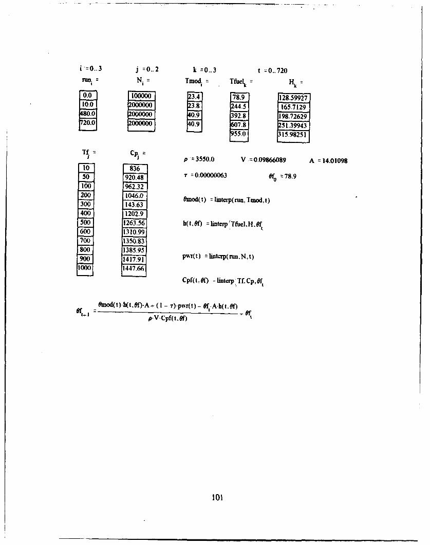
i =0..3 j 0..2 k =0..3 t =0..720run. N.= Tmod. Tfuelk H

0.0 100000 789 128.5992710.0 000000 8 1657129.0 198.72629

7 2 0 .00 0 0 0 0 0 .97 .8 5 1 .3 9 9 4 3

. F1598251

TfCpi cpj p= 3550.0 V =0.09866089 A 14.01098

10 8365O 920.48 7 = 0.00000063 ef0 =78.9100 962.32200 1046.0 Omod(t) :=interp(run.Tmod.t)300 143.63400 1202.9500 1263.56 h(t, f) =Iinterp'Tfuel.H. Oft600 1310.99700 1350.83800 1385.95900 1417.91 pwr(t) lintcrp(run.N.t)

1000 1447.66

Cpf(I -ef) -lintrp Tf, Cp, Of

0mod(t) -b(t.ef).A - (I - i).pw Nr(t) - Oft.A -h(t. If)

p.V.Cpf(t.0f)

101

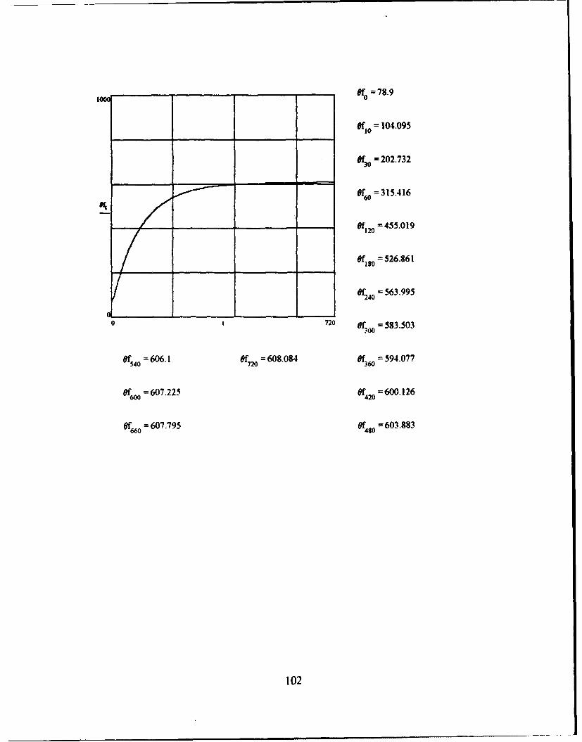
1000_ _ Of = 78.9

eflo = 104.095

"3f0 = 202.732

Of6o = 315.416

otf20 =455.019

Oflso = 526.861

"240 = 563.995

0 720 0f)o = 583.503

8f540 = 606.1 Of720 =608.084 Of36o = 594.077

Of6o0 =607.225 Of420 =600.126

=f66o = 607.795 Of4so =603.883

102

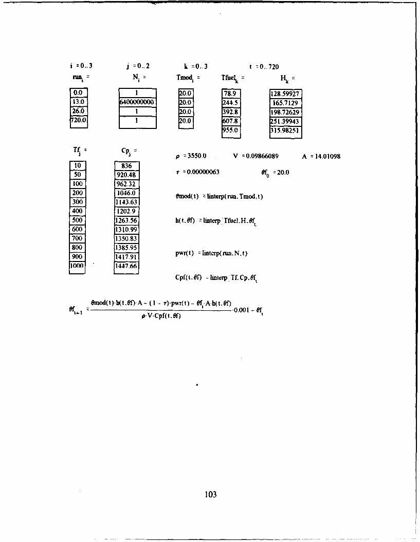
ij =0..2 k =0..3 t =0..720

run,= N. Tmod.= Tfuel Fk

001 78.9 128.5992713.04 2445 165.712926.0 392.8 198.72629

720.0.0 7.8 251.39943955.031.98251

Tf= CpSp p = 3550.0 V =0.09866089 A 14.01098

10 83650 920.48 7 =0.00000063 Ofo =20.0

100 962.32200 1046.0 enod(t) zlinterp(run.Tmodt)300 1143.63400 1202.9500 1263.56 h(t.") linterpl Tfuel. H. Of"600 1310.99700 1350.83800 1385.95900 1417.91 pwr(t) :lntcrp(run.N.t)

1000 1447.66

Cpf(I. Of) - linterp Tf. Cp. Oft

t Omod(t).h(t.0f)A A - (I - 4r)-pw r(t) - Oft.A.h(t.8f)

p.V-Cpf(t.0f)

103

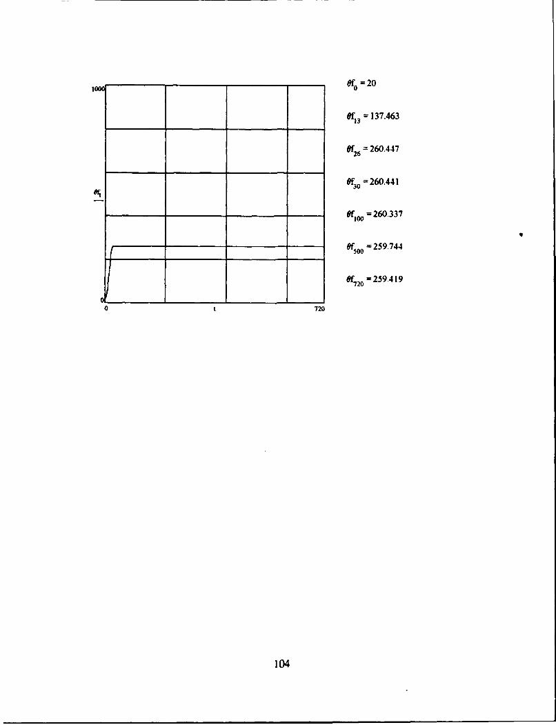
1000 Ofo = 20

6113 = 137.463

K26 = 260.447

af-0 = 260.441

Kim = 260.337

Ifsoo ý 259.744

ef720 = 259.419

0 720

104

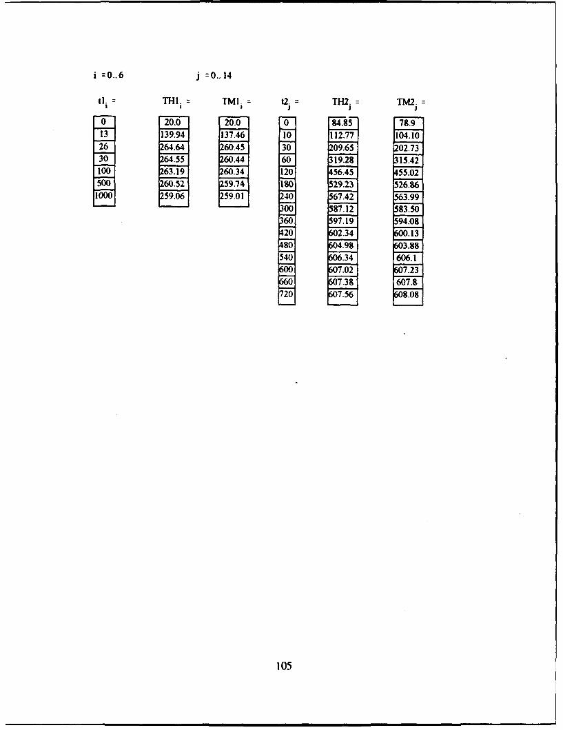
i =0..6 j 0.. 14

ti. = THI. TMI. t2. TH2. TM2.I * !j j j

"0 20.0 20.0 0 84.83 78.913 139.94 137.46 10 '112.77 104.1026 264.64 60.45 30 209.65 202.73'30 264.55 260.44 60 319.28 315.42100 63.19 60.34 120 456.45 455.02500 60.52 59.74 I80 529.23 526.861000 59.0659.01 40 567.42 563.99

300 587.12 583.50360 97.19 94.08420 2.34 .13F80- 4.98 3.88T40 .34 606.1I

7.02 7.237.38 607.8

20 07.56 8.08

105

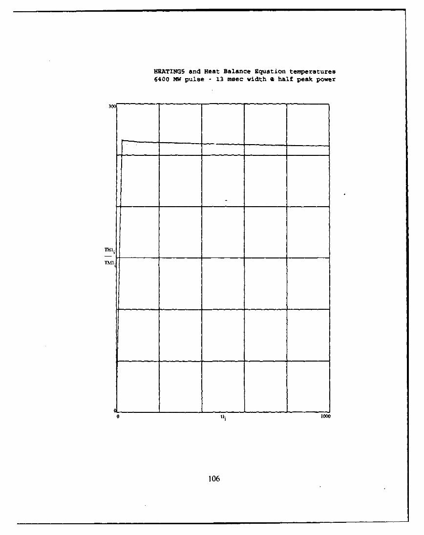
HRATING5 and Heat Balance Equation temperatures6400 MW pulse - 13 msec width a half peak power

30

ml|.

0 Ii 1000

106

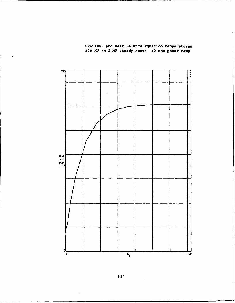
HEATING5 and Heat Balance Equation temperatures100 KW to 2 MW steady state -10 sec power ramp

75o

TM2.

0 720

107

i =0.. 14

radius.- TO. T13.- T26. T30. TIOO. T500.I I I I I I I

i 59 0 27.62 71.4 87.86 209.32 222.91:)0318 0 115.82 217.84 217.9 218.9-2 223.12'

.00522 8.35 222.75--- 222.76' 223.01 225.7

.007305 20 120.7 227.47 227.52' 228.33 231.55

.009367 20 126.09 238.13 238.18 238-86 39.18.01 143 0 134.79 254.67 254.49 251.75 44.06.01181 137.31 260.71 261.05 265.83 [78.6- 1013048 20 142.99 271.16 271.25 273.07 81.25.014285 20 150.45 285.59 285.66 286.6 86.11.015523 20 159.87 303.36 303.28 301.28 289.16.01676 T0 16653 315.02 314.44' 306.36 286.51.01697 20.15 21.06 21.39 25.6 45.017963 20 20.02 20.26 20.42 24.31 43.79.01816 20 20 20 20 20.0- 21.7.01867 2 20 20 20 20.03 21.5

T1000 T2000.1 I

226.8 231.74

226.96 231.82228.94 232.81233.37 234.96

38 15 237.26240.93 238.93

281.96 277.87282.68 277.82282.85 276.33281.36 273.46277.26 69.2964.04 92.3262.87 91.2

125.95 38.0625.59 37.49

108

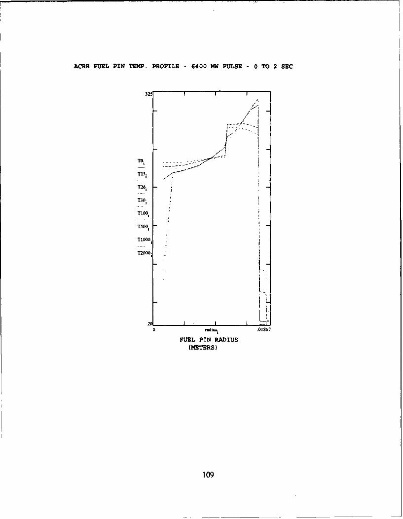
ACRR FUEL PIN TEMP. PROFILE - 6400 MW PULSE - 0 TO 2 SEC

325 1 1 1

Toj

T130

TIOO,

T26O

0 rd .us . . 0.. 6

---

T100i

T500i-

TIO00

T2000

0radiusi .0186'7FUEL PIN RADIUS

(MEJTERS)

109

Aggendix B

Heating 5 Sample Input File - 6400 MW pulse_ _ _II

Heating 5 Sample Input File - 10 second power ramp_ 113

Heating 5 Sample Output File - 10 second power ramp 115

Heating 5 Sample Output File - 6400 MW pulse 151

110

ACRR HEAT DEPOSITION TRANSIENT #1 - 6400 MW pulse- 13 msec vidth la half100 2 8 4 1 1 19 2 1 8

8 10003 1000 Ic-5 1.9 0.001 1.1 0.0 2.01 1 0.0 0.00318 0.03.141592612 2 0.00318 0.01143 0.03.14159261 13 1 0.01143 0.01181 0.03.141592614 2 0.01181 0.01676 0.03.14159261 15 1 0.016760.0169669 0.03.141592616 30.01696690.0179631 0.03.141592617 10.0179631 0.01808 0.03.1415926!8 4 0.01808 0.01861 0.03.14159261 11 HEVOID 5.192e3 -6 -72 FUEL 24.0 3550.0 -13 NBCUP 8570.0 270 -54 SS 7950.0 502 -21 1.0 -3 -41 20.01 1 1.0 -8

1.0 21

0.0 0.00318 0.01143 0.01181 0.016760.01696690.0179631 0.018080.01861

2 4 1 4 1 1 1 10.03.1415926

11 22 1.0 30.27977281 25

10.0 836.80 50.0 920.480 100.0 962.320 200.0 1046.0300.01143.6266 400.0 1202.9 500.0 1263.568 600.01310.9866700.01350.8342 800.0 1385.95 900.01417.9111 1000.01447.66401100.01472.0072 1200.01495.7800 1300.01519.1138 1400.01542.10281300.01562.0266 1600.01384.6900 1700.01604.6870 1800.01624.78661900.01644.9726 2000.01631.4000 2100.01681.5695 2200.01700.22542310.01720.6926

2 420.0 17.3 100.0 17.3 200.0 17.3 300.0 19.0

3 30.010.106046 0.0136.4679e10 0.02610.106046

4 110.00318 0.81 0.004 0.82 0.006 0.84 0.008 0.86

0.01 0.92 0.01143 0.98 0.01181 1.0 0.012 1.00.014 1.1 0.016 1.24 0.017 1.28

5 6

!11

0.0 52.3 100.0 54.4 200.0 56.5 300.0 58.6400.0 60.7 1000.0 72.7

6 1820.0 0.072 M00.0 0.072 200.0 0.115 300.0 0.151

400.0 0.184 500.0 0.218 600.0 0.250 700.0 0.278800.0 0.304 900.0 0.330 1000.0 0.354 1200.00.0004051400.0 0.000455 1600.0 0.000502 1800.0 0.000543 2000.0 0.5792500.0 0.657 3000.0 0.745

7 320.0 0.32828 1200.0 0.16334 2600.0 0.167532

8 20.0 20.0 10.0 20.00.0 0.013 0.026 0.03 0.1 0.5 1.0 2.0

1 10.00001 0.001 0.00001

0.1 1.10

112

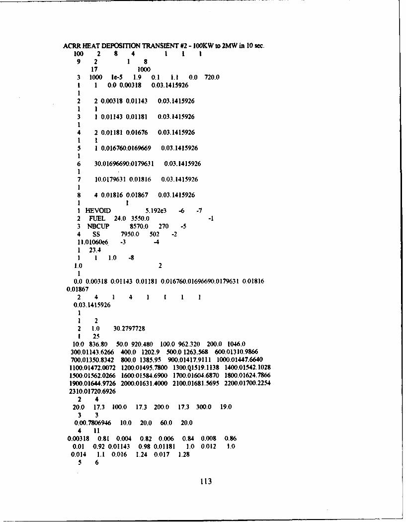
ACRR HEAT DEPOSITION TRANSIENT #2 - 100KW to 2MW in 10 sec.100 2 8 4 1 1 1

9 2 1 817 1000

3 1000 le-5 1.9 0.1 1.1 0.0 720.01 1 0.0 0.00318 0.03.141592612 2 0.00318 0.01143 0.03.14159261 13 1 0.01143 0.01181 0.03.14159261

4 2 0.01181 0.01676 0.03.14159261 15 1 0.016760.0169669 0.03.141592616 30.01696690.0179631 0.03.141592617 10.0179631 0.01816 0.03.141592618 4 0.01816 0.01867 0.03.14159261 11 HEVOID 5.192e3 -6 -72 FUEL 24.0 3550.0 -13 NBCUP 8570.0 270 -54 SS 7950.0 502 -211.01060e6 -3 -41 23.41 1 1.0 -8

1.0 21

0.0 0.00318 0.01143 0.01181 0.016760.01696690.0179631 0.018160.01867

2 4 1 4 1 1 1 10.03.1415926

11 22 1.0 30.27977281 25

10.0 836.80 50.0 920.480 100.0 962.320 200.0 1046.0300.01143.6266 400.0 1202.9 500.0 1263.568 600.01310.9866700.01350.8342 800.0 1385.95 900.01417.9111 1000.01447.66401100.01472.0072 1200.01495.7800 1300.Q1519.1138 1400.015-42.10281500.01562.0266 1600.01584.6900 1700.01604.6870 1800.01624.78661900.01644.9726 2000.01631.4000 2100.01681.5695 2200.01700.22-42310.01720.6926

2 420.0 17.3 100.0 17.3 200.0 17.3 300.0 19.0

3 30.00.7806946 10.0 20.0 60.0 20.0

4 110.00318 0.81 0.004 0.82 0.006 0.84 0.008 0.86

0.01 0.92 0.01143 0.98 0.01181 1.0 0.012 1.00.014 1.1 0.016 1.24 0.017 1.28

5 6

113

0.0 52.3 100.0 -4.4 200.0 56.5 300.0 58.6400.0 60.7 1000.0 72.7

6 1820.0 0.072 100.0 0.072 200.0 0.115 300.0 0.151

400.0 0.184 500.0 0.218 600.0 0.250 700.0 0.278800.0 0.304 900.0 0.330 1000.0 0.354 1200.00.0004051400.00.000455 1600.00.000502 1800.00.000543 2000.0 0.5792500.0 0.657 3000.0 0.745

7 320.0 0.32828 1200.0 0.16334 2600.00.167532

8 30.0 23.4 480.0 40.9 720.0 40.90.0 5.0 10.0 20.0 30.0 60.0 120.0 180.0

240.0 300.0 360.0 420.0 480.0 540.0 600.0 660.0720.0

1 10.00001 0.001 0.00001

0.1 1.1

114

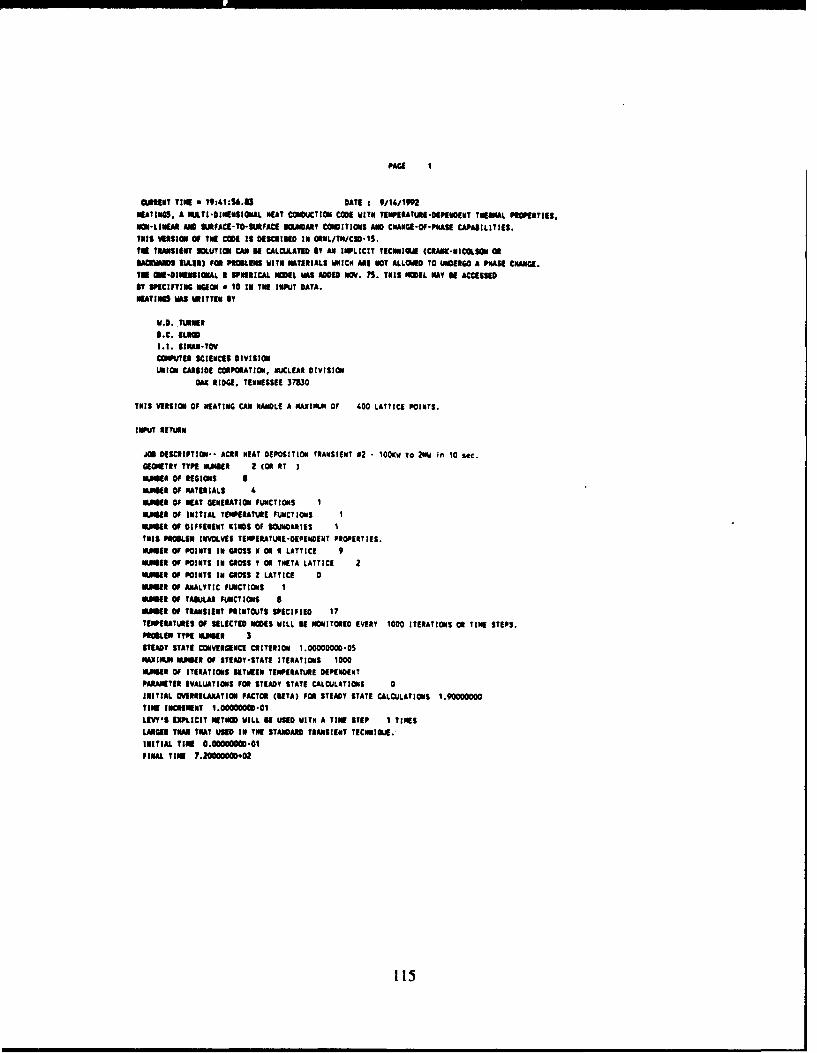
PAGE I

CURRENT TIME a 19:41:A6.0 DATE : 9/14/1992

MEATIHOS. A MULTI-DIMENSIONAL NEAT CONDUCTION CODE WITN TENIERATUEE-OEPENDENT TNEIMIL PROPERTIES.

NON-LIANEA AND SAFACE-TO-SAPACE BOUNDARY CONIDITIONS LAND CHANGE-OP-PHASE CAPABILITIES.?HIS VERSION OF THE MUE IS DESCRIBED IN UHML/TN/CSD-1S.fill TRANSIENT SOLUTION CANBE CALCULATED IT AN IMPLICIT TECmINNUE (CRANK-HICOLSON 0RSAIMMS "itR) PU MPOBLEMS MITI MATERIALS WNIC11 All NOT ALLOWED TO UNIDERGO A PHASE CHANGE.TINK =-DIMENSIONAL I S1PHERICAL NOEL WAS ADDM NOV. 7S. THIS MODEL PAY If ACCESSEDIT SPECIFYING MSGON a 10 IN THE INPUT DATA.0EATINGS WAS WRITTEN ST

W.D. TURNERD.C. ELROD1.1. SINAUI-TOY

CO!PUTER SCIENCES DIVISIONUNION CARBIDE CORPORATION, NUCLEAR DIVISION

OAK RIDGE, TENNESSEE 37830

THIS VERSION OP HEATING CAN RNADLE A MAXIMUM OP '00 LATTICE POINTS.

INPUT RETURN

JOB DESCRIPTION-- ACER HEAT DEPOSITION TRANSIENT 02 - 100KCW to 2MW~ in 10 stc.GEOMETRY TTPE NUMBER 2 (oR RIT I

ULMER OF REGIONS aVW~lR OF MATERIALS 4

IWER OF HEAT GENERATION FUNCTIONS I

ULMER OP INITIAL TEMPERATURE FUNCTIONS INUMBER OP DIFPERENT CINDS Of BOUNDARIES iTHIS PROBLEM INVOLVES TEMPERATURE -DEPENDENT PROPERTIES.

NMBSER oP POINTS IN GROSS H Un It LATTICE 9NUMBER OP POINTS IN GROSS T OR THETA LATTICE 2NUMBER OF POINTS IN GROSS Z LATTICE 0NUMBER OP ANALYTIC FUNCTIONS I

UMISER OP TABULAR PUNCT IONS I

NUMBER OP TRANSIENT PUINTOUTS SPECIFIED 17

TEMPERATURES OP SELECTED NOWES WILL SE MONITORED EVERY 1000 ITERATIONS OR TINE STEPS.PROSIEM TYPE NUMSER 3STEADT STATE CONVERGENCE CRITERION I .00000000-05

MINIMUN NMBER OF STEANT-SIATE ITERATIONS l00

NMBSER OP ITERATIONS SETWEEN TEMPERATURE DEPENDENT

PARAMETER $VALUATIONS PUR STEADY STATE CALCULATIONS 0

INITIAL OVEERELARATION FACTOR (EITA) PUR STEADY STATE CALCULATIONS 1.90000000TIME INCREMENT 1.00000000-01

LEVY'S EIWICIT METNOD WILL N USED WITH A TIME STEP I TIMESLARGER THAN tHAT USED IN THE STANDARD TRANSIENT TECNUISIE.

INITIAL TINE D.0D00000D0-01FINAL TINE 7.ZODD000OD.2

115

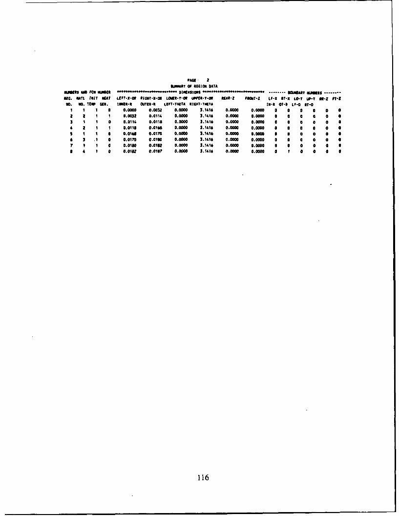
PAGE. 2

*lewt? OF tfGIGN DATA

MIasIt AND FCu IOUNt DIMENIDOS OImfIWlI0NI , *.o,, ........ ONaarY MUNi t ........

IEG. iNTL hINt SLAT LEFT-1-Ot R*GNo-M-u LKI--Of- U& fI-T-Ol ItEA--Z lrrrI- u-X ar-n La-v UD.? W- Z FPS

NO. N0. TINP an. INlN$t-l OUTER-t LIFT-TNETA RICNT-THETA Ili-t OT- Lu-O IrT-a

I I 1 0 0.0000 0.0032 0.0000 3.1416 0.0000 0.0000 0 0 0 0 0 0

a I 1 1 0.0032 0.0114 0.0000 3.1416 0.0000 0.0000 0 0 0 0 0 0

3 1 1 0 0.0114 0.0118 0.0000 3.1416 0.0000 0.0000 0 0 0 0 0 0

4 a I 1 0.0118 0.0168 0.0000 3.1416 0.0000 0.0000 0 0 0 0 0

1 1 1 0 0.0168 0.0170 0.0000 31.16 0.0000 0.0000 0 a 0 0 0

6 3 .1 0 0.0170 0.0ai0 0.0000 3.1416 0.0000 0.0a00 0 0 a a 0 0

1 1 0 0.0180 0.01a2 0.0000 3.1416 0.0000 0.0000 0 0 a 0 a 0

1 0 0.01a 0.0187 0.0000 3. Mo6 0.0000 0.0000 0 f a 0 0 0

116

PAGE 3

SIUlMMY OF MATERIAL DATA *..*..*e*

MATERIAL MATERIAL ............ TNElIML PAAMIETERS ............

NiUMER UKq -- TEMPEiATUl*-OEPENOENT FUNCTION NiUIMBS --

CONOIJCTIVITY DENSITY SPIECIFIC NEAT

I IVOID 0.0000000-01 O.00000-01 5.1920000-03-6 "7 0

2 FUEL 2.4O00000+01 3.5500000.03 0.0000000-01

0 0 -1

3 sD" 0.0000000-01 8.5700000=03 z.7000000*02.5 0 0

4 SS 0.0000000-01 7.9500001#03 5.0200000*02.2 0 0

S AIWMAY OF INITIAL TEIPERATUIE DATA - -ts

NUMBER INITIAL POSITION-OEPENOENT FUNlCTION WIEl[S

TEMPERATURE X ORl a T on TN Z

t 2.340000.0? 0 0 0

..** ..e*@** SUJIARY OF NEAT GENERATION RATE DATA ........ ......

IIUmEI POWER TIME-, TEMPERATU11E- AND POSITION*-DEPENDENT NUMBERS

DENSITY TIME TEMPERATURE X OR IA Y ORl TN Z

I 1.01060D.06 "3 0 -4 0 0

117

PAGE 4~O 09 UNOAS, OAVAý*49*...

*.... ENERAL . TMUTUE....... TE RARJ .............................. ~v "I IsAus TRMI 9P1OEFCIENTS .......................INFORMATIONS BELATEO FUNCTION UM ISS

0O. TYPI Fey TINPERATLME PUomCE, v. RDATIOzNm UATIAAL COM ENOMUT PLUIFLAG A TINE FCT AS$=C.

FCTS

t i .000000.00 i.000000.0 0.000000. O.000000o1 0.000Os-ol 8.00000-01TIME 0 00 0 0TEMP I00 g

GEM8 LATTICE$ AN WMiv 0f INCtEmENTS

0.000000 0.003180 0.011430 0.0118ot0 0.016760 0.016967 0.017963 0.0181600.016670

2 4

yNlTA T1

0.000000 3.141593

L.ISTING 0f ANALYTIC FUNCTIONS

F(V)- A~l) # ACZ)-V - A(3)1"-2 + AC4)COS(ACS)*V) - A16)*EX(PA(l)*V) * A(6)*S11(AC9)*V) - A(tO)*LOG(ACiI)-V)

No. A(i) AM2 AM3 AMs A(S) A(6) A(7) AM8 A(9) AtI0) Atli)10.0000-01 1.0000-00 2.79110-01 0.0000.01 0.0000.01 0.0000-01 0.0000-01 0.0000.01 0.0000-01 0.0000.01 G.0000-0

FAN1 5LISTINGI 0f TABUJLAR FU.NCTIONS

TAKES wUmR ¶ mjUAIR Of PARS - 2

ARGUMENT VALUEI .000000000.01 S.366000000025.000000000.01 9.20880000021.000000000.-02 9.623200000.022.00ooooo00+02 i .084000000.033.000000000+02 1. 1436 6o.038.000000000.02 1.202900000.039.000000000002 1.263S630M0.036.000000000.002 1 .5l09g6w*003?.000OOOOoWo I .3suU0I3'Zo011.0000000010.02 1.35950000.039.000000000.02 1.417911100-03l.000000000.03 I ."7664000-031.100000000.03 1.47200720003¶ .200000000003 I..89780000.031.30000000D.03 1.5191138M#.031.400000000.03 1 .542102800-03I .50000000D.03 ¶ .562026600.031.600000000.03 1.584.690000#031.700000000.03 1.6"1697000.03I .800000000.03 1.624.786600.031 .90,0000000.03 1.6441972600.032.000000000.03 1 .6314.000M0.032.I10000O=003 1.681569"00.032.200000000.03 1.700225400.032.310000000.03 I.720692600.03

TAML NUMBER 2 NUMBER OF PAIRS -

ARGMNmT VAL.UE2.000000000001 1.730000000.011.000000000.02 1. 30000000.012.000000000.02 1.730O000000.013.000000000.02 1 .oooooooo00s)

TABLE NUMBR 3 NUMBER OF PAIRS - 3

ARJSEINT VALUE0.000000000-01 1.000000000.000I .000000000#01 2.000000000.016.000000000.01 2.000000000.01

TABLE EsueR 4 EMBE OF PAIRS 11

3.1800000.038.1I00000000.018.00000000-03 8.a00000000-016.0CM -0 .000000(l0 a80 oooool0.00000000003 8.600000000-01I.00000000.2 9.200000000-011.1430000".02 9.800000000011.181000000.-02 1.000000000.01.200000000-02 I .000000000.01.400000000.02 1.100000000.001.600000000.02 1.24000000.000

119

I .700OM0000o 1.280000000.00

120

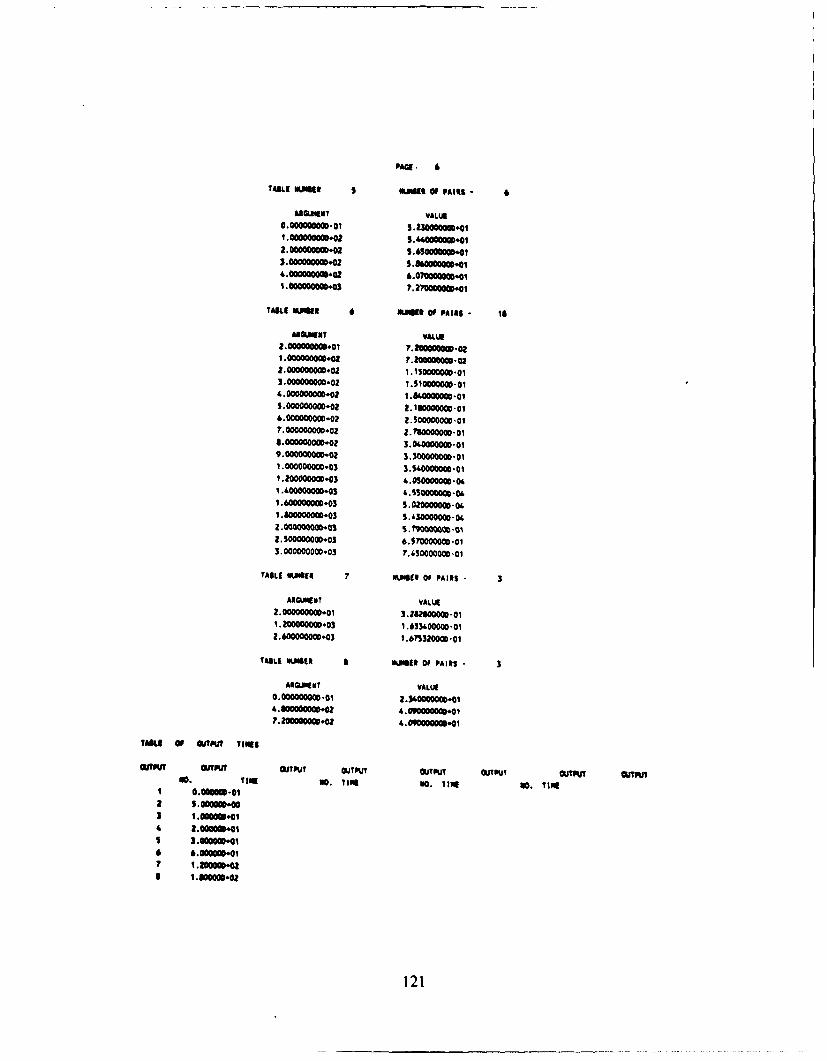
TABL.E 10m.0111 *A" orts PAIRS -

LARGMENT VALUE0.000000000-01 S .230000000-01

1.000000000-02 S.830000000-012.000000000.02 S.6s00000soo¶3.000000000#02 5 .3?000000,

¶ .0000000s0o3 7.270000000.oi

TABLE UMMINE 6 Nmam'tOF PAIRS. Is

ARGUMENT VALUE2-000000000-01 7.20000M000.0

2.000000000.02 I. lS0OOWoao0o

3.000000000.02 1.510000000.01

5.000000000.02 1.I64000000.015.000000000.02 2.160000000-ol6.000000000-02 2.7500000M-oa?.000000000.02 3.04.000oD00009.000000000.02 3.3000000oo-oi9.00000000.02 3.3400000000-01

1.200000000.-03 3.05000000o.011.4.0000000003 4. O30000000-OWL1.400000000.03 4.511000000-041 .6000000M0.03 S .02000000o-042.0O00000000.03 5 .&00o0000.02.S000000000.o3 A.50000M M-01

3.000000000.03 7.4650000000-01

TABLE MillER 7 *MCIE OF PAIRS - 3

AIGUMEW? VALUE2.000000000.oi 3.29260000o-0ai.200000000.03 1.633oL0000-012.600000000.03 1.673320000-Ol

TABLE NMBSER ENUEIN OF PAIRS - 3

ARGISE.? VALUE0.000000000-01 2.34.000000D.01

7. 200000000.02 4..0900000010.o1

TABLE OF OutPul Timis

gflPUT 0~R~ OUTU OTUT OUTPUTy OUTPUT WIPUT JuNO. TIR N. TIME No. I soE . 1t01

2 .0000004003 1.000000.01' 2.000000.01S 3.000009.018 8.000000.0

7 1.2000I

S 1.80M00."

121

9 2.40000-0210 3.00000.02

122

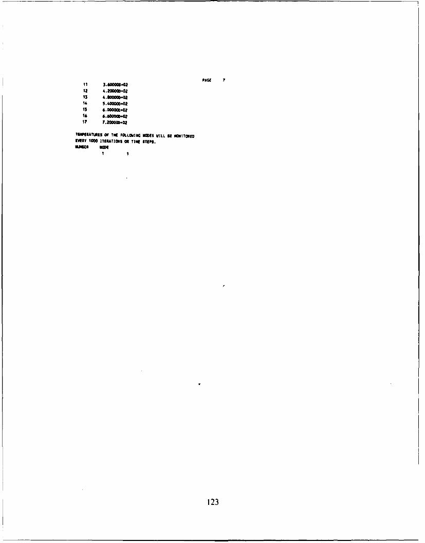
PAGE 7It 3.600000O2

12 4.zoooaoDoa

16 6.IOOOUDOO2

MOT11611TE of ?ME FOLI.SWIUO USEIS WILL U OUItTSEEVERY 1000 ITERATIONS 00 Y1 STEPS.

123

PAGE a

FINE LATTICE. X OR , V OR THITA, AND Z

2 0.001590 3 0.003180 4 0.005242 s 0.007301 6 0.009367? 0.011430 8 0.011810 9 0.013048 10 0.01425 11 0.011i1

12 0.016760 13 0.016967 14 0.017963 1 0.018160 16 0.01870

1 0.000000 2 3.141593

lrIS PROEIN CONTAINS 30 NODES.

124

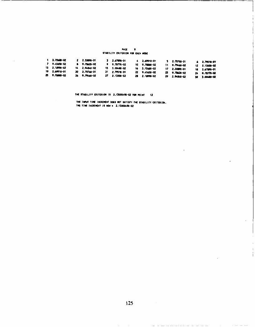
PAGE 9STABILITY CuITERuO FORl IACN MOE

I 3.?26D-02 I 2.3OgmO- 3 2.67S9-1O 6 2.69910-01 S 2.70740-01 6 L.YS1-0I7 9.a5650-02 3 9.71620-02 9 9.78770-02 10 9.7110-02 11 9.7960-02 12 2.130O3-W

13 2.1t9-02 14 2.984o-02 Is 3.00D-02 16 3.72610*02 17 2.30am-o1 1 2.67090-0119 2.69910-01 20 2.,0740-01 21 2.70510-01 22 9.45650-02 23 9.71620-02 26 9.71170-0225 9.71010-02 26 9.7060-02 27 2.13030-02 28 2.19s0-02 29 2.94440-02 30 3.00"D-02

TME ITASILITY CRITERIO I 2.13000490-02 Fn 60IT 12

TN[ INPUT TIME INUCEMNET DOS NOT SATISFY TNi STAiILITY CRITERION.tIN1 TINE INCIEMENT IS Nw . 2.13000.40-02

125

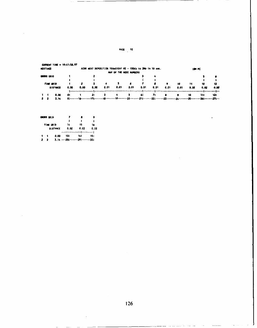
PAGE 10

MURENT TIM E 19:41:50.97NEATINO ACAI NEAT DEPOSITION TRANSIENT 02 - I01K to 2iM in 10 sec. [im PC

NAP OF TNE NODE IIURS

GOSS IO 1 2 3 4 5 6

FIRE dat 1 a 3 4 $ 6 7 8 9 1* 11 12 IsDISTANIC 0.00 0.00 0.00 0.01 0.01 0.01 0.01 0.01 0.01 0.01 0.02 0.02 6.01

I ................. I .................................. I .......... I .......................... I ........ I..1I 0.00 O0 1 21 3 4 5 61 ?1 a 9 10 111 111

2 2 3.14 01 ...... 16 ....... 171 ...... 10 ....... 19 ....... 20 ....... 211 ...... 221 ...... 23 ....... 24 ....... 25 ....... 261 ...... 2--

GROSS MID 7 a 9I I I

FINE AIIK 14 Is 16

OISTANCE 0.02 0.02 0.02

- - -I.K.. K..1 1 0.00 131 141 151

2 2 3.14 --- 281 ...... 291 ...... 301

126

PACE 11

CURRENT TINE a 19:41:59.35RIATINGS ACt NHEAT DEPOSITION TRANSIENT 5? - IOOR to bW in 10 seC. IN PC

STEADY STATE TIE5ATIURAE DISTRIBUTION AFTER 0 ITERATIOUS. TINE * 0.000000-01

ROSSIO 2 1 4 S 6I I I I

PIm RID 1 2 3 4 5 6 7 8 9 10 11 12 Is

DISTA VC! 0.00 0.00 0.00 0.01 0.01 0.01 0.01 0.01 0.01 0.01 O.0z 0.0 0.02I ................. I ................................... I ........ I ................................... I ........ I..

I 1 0.00 0.00 23.40 23.40 23.40 23.40 23.40 23.40 23.40 23.40 23.40 23.40 u3.4 n.402 2 3.14 0.00 .... 23.40 .... V3.40 .... 23.40 .... 23.40 .... 23.40 ---- 23.40 .. 3.40......40..... - .40 .... 23.40 .... z3.40o.....&4

OSSOmIO 7 8 9I 1 1

rINE GRID 14 15 16DISTANCE 0.02 0.02 0.02

............... I ........ I

I 1 0.00 23.40 23.40 23.40

2 2 3.14 ...23.40 .... 23.40 .... 23.40

W•PE•W ATURIS ON NUMBEREED OUNOARIES

BOUNUDAR NMuER TEM[EATU5E

1 23.400000

TWE NAXIMU TEMPERATURE iS - 2.340000.01 (+-0.1)

MAN. TEMP. APPEARS AT MUOES 1 2 3 4 s6 7 a 9 10

11 1z 13 14 1i16 17 18 19 2021 22 23 24 25

26 27 26 29 30

TME NINIUM TEEMPRURE IS - 2.340000.01 (*-0.1)

11h1. TENP. APPILARS A' IN•DS 1 2 3 4 56 7 a 9 10

11 12 I3 14 1516 1? 1 19 2021 22 23 24 2526 27 28 29 30

127

PAGE 12MAIN TME STEADY STATE CALCULAT IONSNUMBE OF EXTRAPOLAT ION

ITERATIONS CONWRIaGECI 111"TEEATUWI FACTOR

5 5.46246-02 17 2.403491.0 -3.232351.010 6.252S29-02 16 3.1383EM.01 -3.905361.001s 3.965531,02 I 3.71002[.01 *9.967321.020 2.501IS99-02 2 4.31600S.01 9.994651+00as 2.031426102 1 4.7S9581.01 3.123906.030 1.613691-02 16 S.24227141l 1.743ww.035 1.3627¶E-02 I 5.391371.01 -1.522751.03'0 1.1?5131-02 7 4.714841*01 9.S22441*01

$ETA REDUCED TO 1.30045 8.155751 -03 1 6.220471-01 2.358441.01so 5.409341-03 I 6.384631.01 4.U3E931005S 4.730441-03 16 6.558416.0 A.a0241t.0060 4.422791-03 16 6.7046S1.Ol -9.229301*01

$ETA REDUCED To 1.70065 3.357821-03 1 6.813181-01 4.239911.0170 2.449001-03 1 6.90022E-01 1.345M0.0175 2.395451-03 2 6.99502S-01 2.22192t.01so 2.293441- 03 1 7.067011.01 2.230241.02

MEA REDUCED TO 1.600as 1.833349-03 1 ?. 137081.01 5.273371.0190 1.555751-03 1 7.l19151E.01 4.20859E-0195 1.46%9E9-03 2 7.ZS2121.01 *.s5720t.0t100 1.425931-03 1 .297871.01 1.94763E.02

$ETA REDUCED To 1.500105 1.16M79-03 I 7.34332E.01 6.274071.01110 1.033386-03 1 7.38092E.01 2.341981.02115 1.0000&E-03 I 7.41926E-01 1.96929E.02120 9.80431E-04 7 5.86274E.01 3.107'72E*02

EXTRAPOLAT ION125 -6.085271-04 14 4.15969E.01 1.441361*0l130 -3.997m8-04 14 4.149781.01 1.126861.0I135 -2.64458-04 14 4.14327E-01 1.1799SE.0l140 -1.766911-04 14 4.136921.01 1.251371.01

EXTRAPOUTION145 -6.11265E-05 1 9.676616.01 5.473771.01ISO -5.593411-05 1 9.674011.01 5.639661.01155 -5. 1354691-0 1S 9.67.U/.1.01 5.693351.01160 -I.7?34091-05 1 9.671071.01 6.20495E.0I

EXTRAPOLATION165 -3.066711-05 ? .661691.01 4.544301.01170 -2.77318-05 7 7.640591.01 S.IM3406.0175 -2.538171-OS 7 7.059581.01 5.38W232.0IS0 -2.347241-05 7 7.06041.01 4.657361.0

EXTRAPOLAT ION185 -2.&IN1221-05 27 5.742172#01 2.?4IQ5l~oIM9 -2.123511-Os 27, S.WS121.01 3.237=21.0

195 *1.854391-05 2? 5.740961.0 3.034409-01200 -1.672&41-05 1 9.633361.01 6.977541.01

EXTRAPOLATION25 -1.78555-05 22 7.644I851.0 3.758601.01

Z10 -1.580341-OS 22 7.641211.01 4.248781.01215 -1484-S 22 7.440651.01 4.801171-01220 -1. 288681-OS 22 ?.66014.1.01 5.422310140

EXTRAPOLATION22S -1.3S0621-05 21, 5.733011.01 2.730911.01

128

230 *11~UE05 27 S.7U66401 3.243'4.0l

129

PAGE Is235 *i.0aaus-0s 27 S.7IflM.O1l 3.0600"001

130

PAUE 14

CMIIIT TIME a 19:42,16.63MATIKOS ACm EAYT DPOSITION TIANSIENT i2 - C0OEV tO fl nA 10 8W. IN PC

STEADY STATE TUMIRATURI DlS1MOIUTIO AFTER 236 ITERATIONS, TIME 0 0.000000-01

GR0 1 2 3 4 $ 6I i I | I

FIa ERIC I 2 3 4 5 6 7 0 9 10 IT It 13DISTNiCE 0.00 0.00 0.00 0.01 0.01 0.01 0.01 0.01 0.01 0.01 0.02 0.03 0.02

I ................. 1-1 ................................. I ........ I ................................... I[ ........ I..

I 1 0.00 0.00 96.18 96.10 96.13 96.00 9". 7 "3.52 76.35 76.15 7S.91 75.65 75.3V•2 17.

2 2 3.16 0.00 .... 96.18 .... 96.18 .... 96.13 .-.. 96.00 ... 79. 95.51 .... 76.3S .... 76.15 .... 75.91 .... 75.65 .... 7S.3 .... S7.32

GROS GRID 7 8 9

I I IFINE GRID 14 I5 16

DISTANCE 0.02 0.02 0.02

" .......... o..|I ........ I

1 1 0.00 57.21 41.17 41.00

2 2 3.14 ... S7.21 .... 41.17 .... 41.01

TENPERATLIRES ON MtMBI RID OiCtARI[S

BOUIDOARY NUMBER TENPPRATURE1 23.400000

IVA WISU TEIRAITURE IS 9.617M30-01 (.-0.1)

NAX. TIPP. APPEARS AT ONES 1 2 3 16 17

TME NMINIIM TENPERATURE IS- 4.100480-01 (-o0.1)

MIN. TEMP. APPEARS AT 0ES - IS 30

TIN STEADY STATE CALCULATIONS HAVE £1401 CONPLEIMI.

JU(MIR Of ITERATIONS COMP.LETED s 236

131

PAME Is

O¢uEWT TIME * 19:42:19.18

gATIUS AdS NEAT DEPOSITION TRANSIENT 02 - 100KV to )u in 10 on. ito PC

T14ASIEIT TEIIPAI[TE DISTRIBUTION AFTER I TIME STEPS, TIME 2 2.10100-02

GRSS*ID 1 2 3 4 S 61 I 1

PIM olo 1 2 3 4 S 6 ? a 9 10 11 12 13,ISTAMC 0.00 0.00 0.00 0.01 0.01 0.01 0.01 0.01 0.01 0.01 0.02 0.0 01.

I ................. I ............................. I . I ............................. I. I.

I 1 0.00 0.00 96.18 9.IS 96.13 96.00 9..79 95.52 76.35 76.15 75.91 75.6s 75.34 S?.5a I 3.14 0.00 ... 96.1 .... 96.1- - .... 96.13 .. 96.00. .9.79 .... 95. ..... 76.35 .... 76.15 .... 75.91 ---. 75.65 .... 75.3 .... T7.32

GROSSEIS 7 St 9

FINE GRI0 14 15 16

DISTAM" 0.02 0.02 0.02

I 1 0.00 57.21 41.17 41.00

2 2 3.14 ...-5?.2.---.41.... 41.01

TEMPERATURES ON WJUlRED BOUNDARIES

DOUMONSY UMBER TEMPERATULRE

1 23.400766

TWE CURRENT TINE STEP (DILTAT) * 2.101862660-02

INS PAIXMU TEMPERATUIE IS - 9.617B0D-01 (.-0.1)

MAX. TEMP. APPEARS AT MODES - 1 3 16 17

TN MINIMUM TEMIPEATURE IS - 4.•1004.01 (-'0.I)

WIN. T10P. APPEARS AT OWES Is 30

132

PAGE 16

CUAME1t TIME a 19:42:46.70

09ATINGS ACRA HEAT DEPOSITION TRANSIENT 2 - I00V to 2W in 10 soc. [IN PCTRANSIENT TEMPERATURE DISTRIOUTION AFTER 238 TIME STEPS, TIME 5.O017i0rO0

0ms GatO 1 2 3 4 5 6I I

FI GmID 1 2 3 4 5 6 ? a 9 10 11 12 1s

DIStANCE 0.00 0.00 0.00 0.01 0.01 0.01 0.01 0.01 0.01 0.01 0.02 0.02 *.UI ................. I ................................... I ........ I ................................... I ........ I..

I 1 0.00 0.00 102.17 1oz.26 102.25 102.24 102.16 101.98 84.17 64.01 .33 £3.58 43.U 36.,T

2 2 3.14 O.00--* 102.17-*- 102.2- ... ---2-29 ... 1 62.16--- .... 44.01 .... 23.82 .... 1.S8 .... 0.2 .... M.72

GROSS GRI0 7 0 9

1 ! I

FINE GRID 14 15 16

DISTANCE 0.02 0.02 0.02.......... •.... Il ........ I

1 1 0.00 58.59 41.41 41.24

2 2 3.14 ..-58.9 .... 41.41 .... 41.24

TEMPERATURES ON MUIRDEREDO OUNDOARIES

SOUNDART MUSER TEMPERATURE

I 23.582354

THE CURRENT TIME STEP (DELTAT) - 2.100736600.02

THE MAXIUM TEMPERATURE IS- 1.022790-02 (4-0.1)

NAX. TYEP. APPEARS AT N0O0ES 2 3 4 17 1I

19

THNE 01Ull TEMPERATURE IS- 4.123690D01 (0-0.1)

MIN. tEWM. APPEARS AT %ME$ S is 30

133

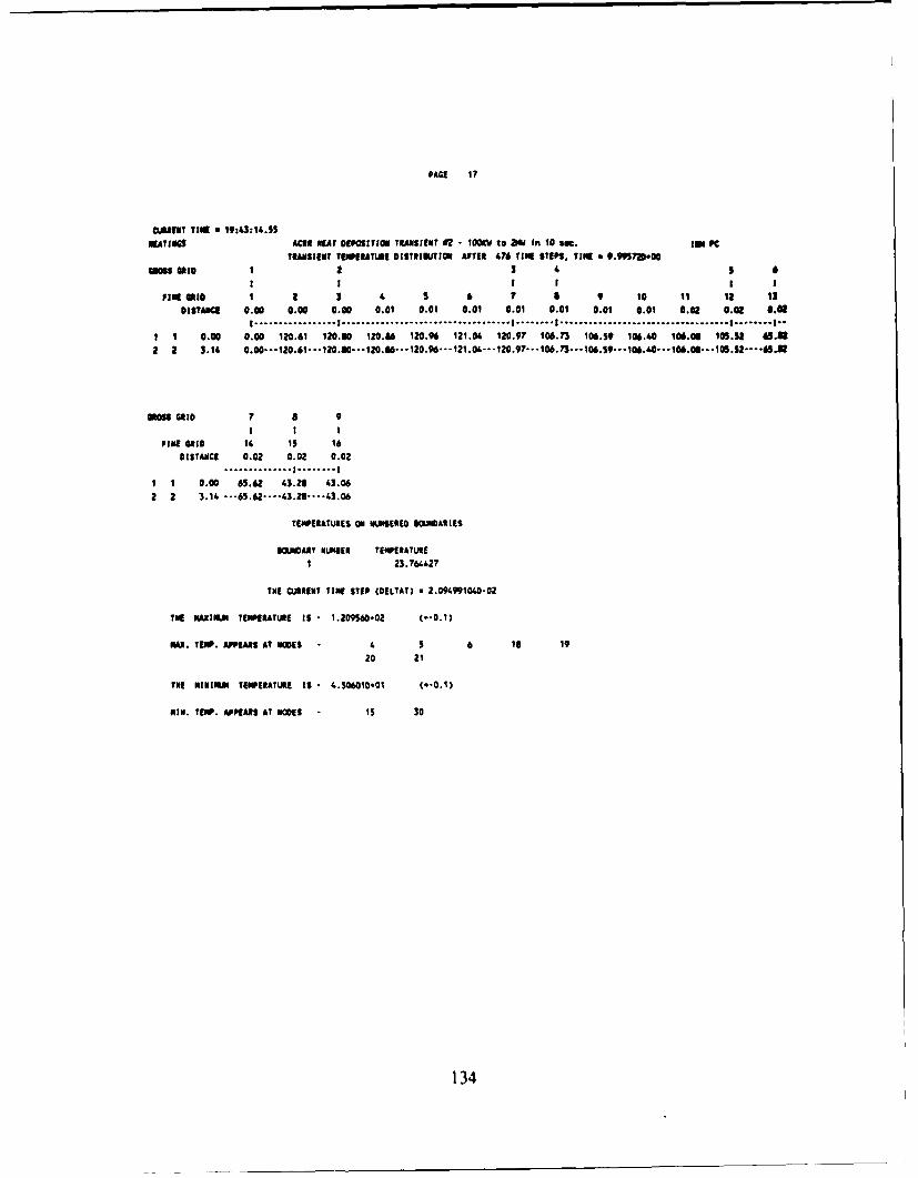
PAGE I?

C0t3I3T TIIME 19:43:14.55

IEATIIGS ACER NOAT D(POSITION TRAMSIENT 02 - O00wV to 20 in 10 s¢. Im PCTRAISIENT TEIMPRATUIR OuSTRIIJTIOU AFTER A76 TINE STEPS, TINE a 9.9J3'9DO00

MOs outo 1 2 3 4 5 6! I I I I I

FI GRID I 2 5 4 S 6 7 a 9 10 I1 12 is

DISTANCE 0.00 0.00 0.00 0.01 0.01 0.01 0.01 0.01 0.01 0.01 0.02 0.2 c.a

I ................. I ............................. I . I ............................. I. I--

I 1 0.00 0.00 120.61 120.30 120.86 120.96 121.06 120.97 106.73 106."9 106.40 106.03 109.52 65.u2

2 2 3.14 0.00--* 120.61- -*120.80- ... 120.6-- 120.96% - 121.04- 120.97---.106.73 ..•- 106.39-.. 106.60..- 106.08---105.S52.----. M5

am GRID 7 8 91 1 1

FINE GRID 14 1 16

DISTANCE 0.02 0.02 0.02

, * * -* * . . . . . .* -| . . . . . . . . I

I 1 0.00 65.62 43.28 63.06

2 2 3.1 ... 65.62 .... 43.28 .... 43.06

TEMPERATURES ON U£I[RENO SOJNARIES

CUQNOATY NOS3ER TEMPERATURE1 23.76?627

THE CURRENT TIME STEP (DELTAT) - 2.094991040-02

THE MAXIUM TENPERATUSE IS 1.209960-02 (+-0.1)

NON. TIP. APPEARS AT NODES 4 5 6 Is 19

20 21

TIE MINIMiU TEPERATURE IS 4.306010.01 (0-0.1)

NIIN. TEMP. APPIEAS AT OWES 15 30

134

PAGE Is

cutm? TIME a 19:66:10.51

SATINOS ACES NEAT DEPOSITION TRANSIENT 12 - 10OK to bW in 10 ao. ito PC

TRANSIENT TEENRATURE DISTRIIUTION AFTERI 9S6 TINE STEPS. TINS * 1.9950.-01

41w180, 1 2 S 6I I I I

FIL int 1 2 3 4 S 6 4 9 10 11 12 13

01STANiC 0.00 0.00 0.00 0.01 0.01 0.01 0.01 0.01 0.01 0.01 0.02 0.02 0.82I ................. I ............................. I . I..................... I ........ I."

I 1 0.00 0.00 169.56 169.70 169.73 169.92 170.06 170.04 160.52 160.32 159.90 '19.21 156.13 95.86

2 2 3.14 0.00--* 169.5S*-- 169. ... 160. ... 169.92---.1V0.06 -- 170.04-*- 160.522--. 60.3--- 139.90--l". ...-3511.$3-..5446

GROSS GID ? 8 9

I I IPINE GRID 14 Is 16

DISTANCE 0.02 0.02 0.0?

I 1 0.00 ..49 S2.96 S2.54

2 2 3.14 --- ".49 .... 5296 .... 52.54

TENMPEATURES ON MNIENED 8aJNOARIES

S ART HUGIE* TEMPENAVURE

1 24.128984

TNE CURRENT TIME STEP (DELTAT) - 2.068856760-02

T I MAZIMUM TNPEATURE IS" 1.70059D-02 (.-0.1)

MAX. TEMP. APPEARS AT OW1ES 5 6 20 21

TNll MINIMLI TEMPERATURE 1S 5.25424001 (.-0.1)

11111. 7101. APPEARS AT VM0S 1 30

TAILE FPl SPECIAL MONITORING Of TEMPERATURES

orI 0F TINS t...e......esstsslllwltt.tl..Ss te 5001 NdMfS N0AN TENPERATURES es..I.Iafl tinHINM~iin

TINM STEPS

1000 2.09050-01 1 1.7392w002

135

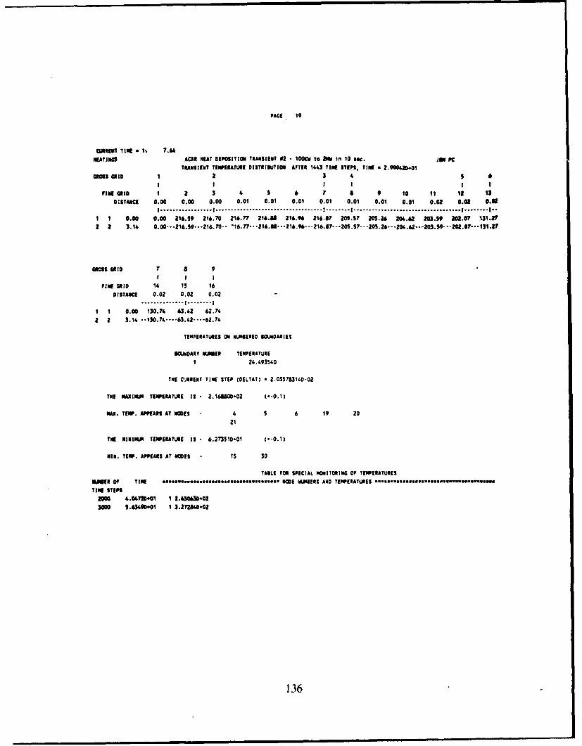
PAGE 19

CURENU TIME ' 1 7.66NEATINGS ACAR NEAT DEPOSITION TRANSIENT 02 - O0i to 211 in 10 $¢.. IN PC

TRANSIENT TIENRATULE OISTRIBUTION AFTER 1"43 TINE STEPS, TINE m 2.9994D.01

gaOs Clio 1 2 3 4 'I I I I I

FINE on 1 2 3 4 5 6 7 1 9 10 11 12 113

OISIAMCE 0.00 0.00 0.00 0.01 0.01 0.01 0.01 0.01 0.01 0.01 0.02 0.2 0.02I ................. I ............................. I . I................... I ........ I..

I 1 0.00 0.00 216.59 216.70 216.77 216.0 216.96 216.67 209.57 205.26 204.62 20.59 202.07 131.2?

2 2 3.14 0.00-..216.59-..216.70-- '16.r?- .-216.88.-- •216.96- -. 216.87 ..- 20$.S7 -.--205.26 ...- 0.62-...203.S9--242.0?... 131.V7

a lS IClO 7 a 9I I I

FINE 0D10 14 15 16

DISTANCE 0.02 0.02 0.07

S.........*..... I ...... I -1

I 1 0.00 130.74 63.42 62.74

2 2 3.14 -- 130.74 .... 63.42 .... 62.74

TEMPERATURES ON NUIMERED BOUNOARIES

BOJUNARY NIMB•l TEMPERATURE1 24.493540

TNE C'.REERT TINE STEP C0ELTAT) a 2.035783160-02

TNE NAXIMU TEMPERATURE IS - 2.16880002 (*-0.1)

NMA. TEMP. APPEARS AT NO0ES - 6 19 20

21

Til NMINI"U TEMPERATURE IS - 6.273510.01 (--0.1)

NIN. TENP. APPEARS AT NMOES 15 30

TAMLE FOR SPECIAL ONNITORING OF TENPERATURES

SIUM# OF TINE .a.hf...a. v.....a.........s..ssa NODE NJUMBES AND TENPERATURES ...... s..... ....... s..n .

TINE STEPS2000 4.0r70*.01 1 2.630630.02

30100 9.634"01 1 3.2724•+002

136

PAGE to

CURRENT TIN[ * 19:08:41.63

NEATINGS ACRI NEAT 0EPOSITION TRANSIENT 02 1001M to 2MW in 10 see. is" PC

TRANSIENT TEMPERATURE DISTRIWTION AFTER 3S2 TINK STEPS, TIM a 6000600.01

ca omno 1 2 4 5 6! I I I

Irlut GID 1 a 3 4 5 6 a 9 10 11 It 13OIST1ICX 0.00 0.00 0.00 0.01 0.01 0.01 0.01 0.01 0.01 0.01 0.03 0.03 8.03

I ................. ................................. I . I..................... I ........ I".

1 1 0.00 0.00 31.0S 361.1 31.06 360.77 360.26 339.37' 305.06 306.87 303.36 301.23 304.41 0.57

a GRI0 7 8 9I I I

FIN GRID 16 i5 16

01STANCE 0.02 0.02 0.02""*°-° *** I ....... OI

I 1 0.00 2013.6 84.82 83.292 2 3.16 -- 201.56-...86.82 .... 3.29

TEMPERATURES ON NMERWSED lOJNDARIES

ISIARIT wimuE TEMPERATURE1 25.511"51

TIE CURRENT TINE STEP (DILTAT) * 1.60997260-02

INS MAXMLU TEMPERATURE IS" 3.110520,02 (--0.1)

NMA. TEMP. APPEARS AT NEES 1 2 3 16 1718

INS NININi TEMPERATURE IS 8.328510.01 (0-0.t)

MI1. tEMP. APPEASS AT MODES 15 30

TAKILE 3 MST IN EVALUATED FOR 6.000879%0.01

TiN VALUE 0F TNS NIrNCTIO WILL IE 2.000000000.01 FOR ALL AJIGUENTS GREATER TAN 6.000000000-01

TAIL[ 10U SPECIAL OMITORING OF TEIPRATURES

RimI os TIme 0s1m.sm m sm..s.,i. *sOS NUMiERS A TEIMPRATURES *uU..... m.

Y IN Sreps

5000 7,.8 01 1 61661500024000 9.3701.01 1 6.66610007000 1.06300-03 1 6.769610.02o0 1.16349.02 1 5.003350#02

137

PAGE 21

CURRENT T1IM a 19:59:,20.90

2ATIUG5 ACON NEAT DEPOSITION TRANSIENT 82 - lOOKW to mW 1" 10 e¢. tom PCTIRANSIENT TEMPERATUIE O6ITIIOUT1001 AFTER 58SW TIME STEPS. TINE a 1.1999D40

M06S GRID 1 2 3 4 5

FNE RID 1 2 3 4 5 6 7 1 9 10 it 12 13

DISTANCE 0.00 0.00 0.00 0.01 0.01 0.01 0.01 0.01 0.01 0.01 0.02 0.02 6.42I ................. I ................................... I ...... I ......................a............ I ........ I.-

1 1 0.00 0.00 $12.47 512.49 511.95 510.48 500.13 04.00 421.23 418.60 41S.26 411.19 400.5 215.732 2 3.14 0.00-...$ ---. 1.49--.. - O--13---$04...---1.23---418.60---415.28---611.11--406.n*...

0EMill 7 8 9GRSaGI a a

PaRE CRt0 11. 15 16

OISTANCE 0.02 0.02 0.02...... o........ I ........ *I

I 1 0.00 274.02 104.47 1013.72 2 3.14 -- 274.02-. 104.47 .. 101.•3

TEMPERATURES ON 4UNIWEREO SOJUNOARI

BOUNDARY PSER TEMPERATURE

1 27.?74934

THE CURRENT TaME STEP ODELTAT) a 9.566938670-03

THE MAXIMA TEMPERATURE 1S - 5.124690D02 (.-0.1)

MAX. TEMP. APPEARS AT MO0ES 1 2 16 17

TM NIMILU TEIPERATURE as- 1.01T270-02 (0-0.1)

MIN. TEMP. APPEARS AT MODES IS 30

TAILE FOi SPECIAL MONITOINGO OF TENPERATURES

MER Of TIME ees ... as ..w.oe.......so-sou........ NI NUMBERS AND TEMPERATURES *S..S.3il ..• .. 3•..S.

TIN STEPS

9000 1.590.02 1 5.205270-02

10000 1.3320102 $ S.38147002

11000 1.42160*02 I 5.53632D#02

12000 1.50170002 1 5.671325002

13000 1.5966*02 1 5.79SO6#02

14400 1.67r0Do 1 11.903950.02

15006 1. r75040o 1 6.001670.02

138

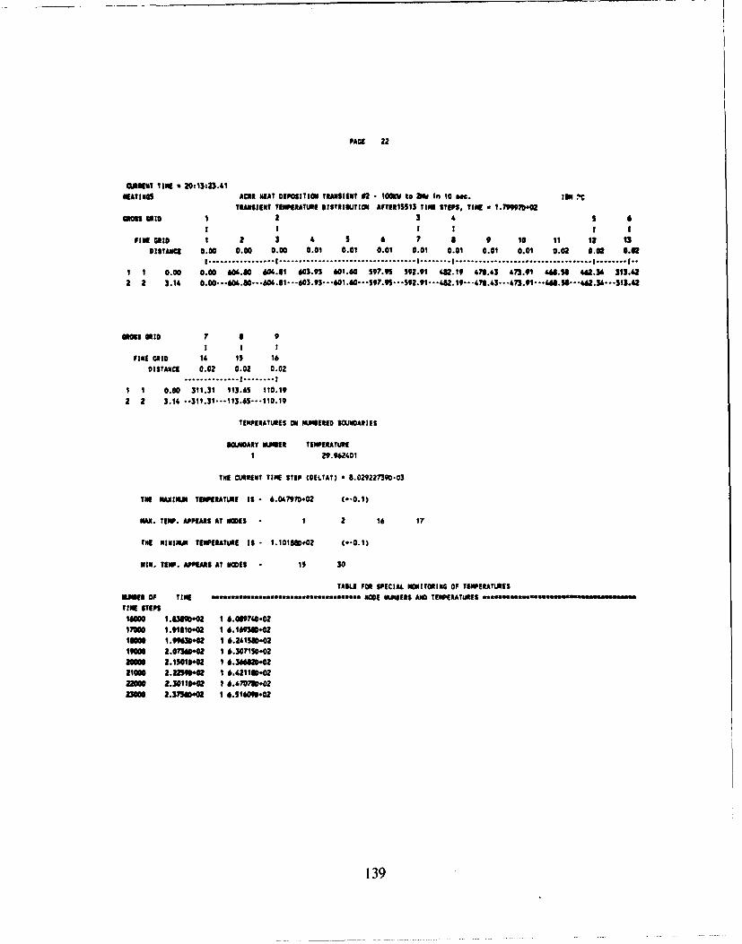
PAGE 22

CIOIST TIME a 2003:23.41NIATINlS ACM NEAT OEPOSITION TRANSIENT •2 - IO•[ to bN in 10 n. isl 'I

TRANSIENT TEMPUATURE OISTRISlUTION AFTERISSIS TIME STEPS, TIME a 1.799970.0salejO 1 2 3 4 S 6

I I I II I

FIu M10 m 2 3 4 ' 6 ?7 a 9 10 11 12 13DISTANCE 0.00 0.00 0.00 0.01 0.01 0.01 0.01 0.01 0.01 0.01 0.02 0.03 0.03

I ................. I ............................. I . I..................... I ........ I..1 1 0.00 0.00 606.80 604..1 603.93 601.60 597.9" 592.91 432.19 478.43 473.01 4643.1 462.36 31S.42 2 3.14 0.00-...60.80---604.81--- 63.93---601.60*--.9W.9--492.91--- 82.19---478.43---4T3.91-...4 ---. 62,U ..- 313.2

MSIDS 610 7 1 9! I I

FINE GRID 14 1s 16

DISTANCE 0.02 0.02 0.02

"*oo*o*' ........ I ........ I

I 1 0.00 311.31 113.65 110.192 2 3.14 --311.31 ... 113.65-.. 110.19

TEMPERATURES ON NUMBERED BOUNDARIES

NONOARY NUMSER TEMPERATURE1 29.962401

THE CURRENT TINE STEP (OILTAT) 8 8.029227390-03

TME NAXIUM TEMPERATURE IS- 6.047970.02 (0-0.1)

WAU. TEMP. APPEARS AT NONES - 1 2 16 17

THE MINIMUM TEMPERATURE IS- 1.10181D#02 0-0.1)

MIN. TEMP. APPEARS AT NONES Is 30

TAILEI FOR SPECIAL MONITORING OF TEMPERATURESomE OF TIE NnMI.mnlalalnlallv.fll.lall. NO i [MEfS AND TEMPERATURES aei n. u..., .iTIME STEPS16000 1.41190002 1 6.09740-0217000 1.9181D02 1 6.169380.02lo0w0 1.993•00 1 6.24151.*0219000 2.0730#02 1 6.307150.02

0010 2.15010002 1 6.3646120*0221000 2.2250I.02 1 6.421110-022200 2.30110.0 1 4.6107100.022O300 2.375400 1 6.516090002

139

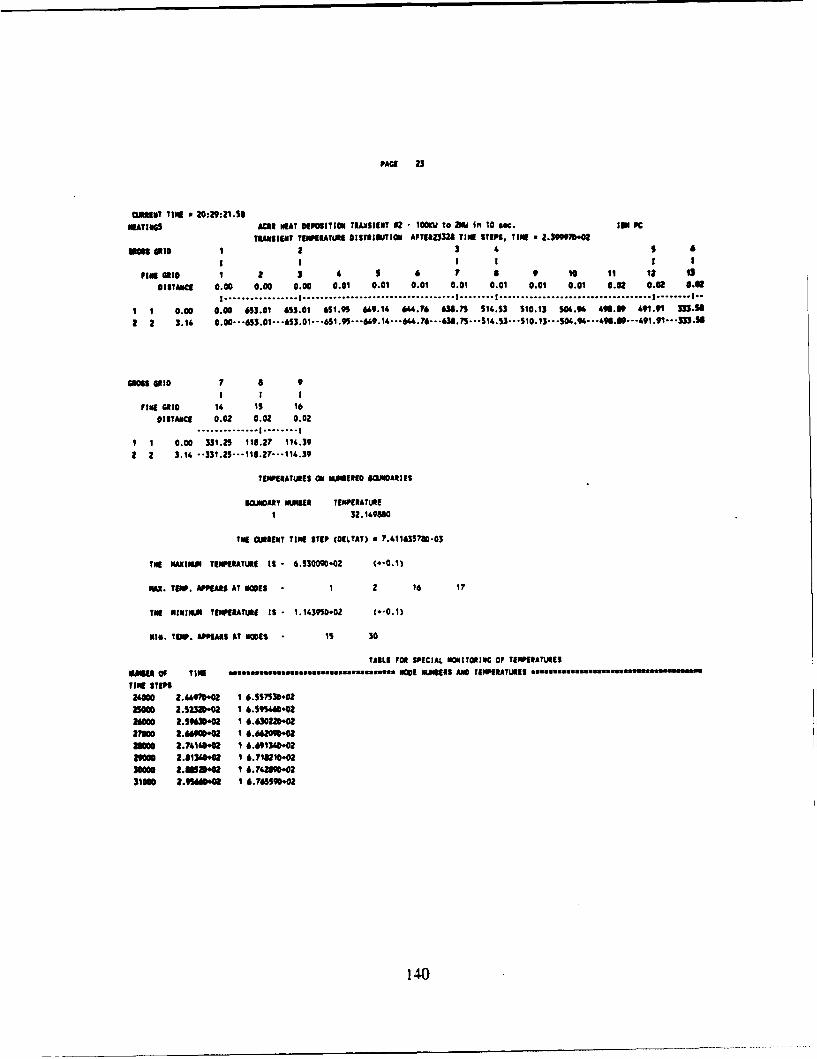
PACE 23

EWIEM? IlN a 20:29:21 .58MATINGS ACIR NEAT DEPOSITION TRASIENT 12 - 00KU to 2NU in 10e IN PC

TRANSIENT TEMPERATURE DISTRISUTION APTERt2332 TIME STEPS. TIME - 2.3999Th.@

11m OntoI 1 2 S 4 5 6

I I I I I

FlgIntoI 1 2 3 4 6 ? a 9 19 11 ii 2 is

DISTANCE 0.00 0.00 0.00 0.01 0.01 0.01 0.01 0.01 0.01 0.01 0.02 0.02 0.01

I ..... *... .................a.............. I........ I..............a..................... I........ I.

I t 0.00 0.00 6113.01 6153.01 651.9" "9.14 644.76 638.7S 514.53 S10.13 S04.96 4U.09 491.91 33.3

a 2 3.1' 0.00 ... 653.01 ... MAI.0l.S... 69 .644. 76 ... 38.?S .. SUM.. S1S0.15 .. 04.94-4911.00..491."---33$.S

005501 7 8 9I I

FINE GrID 14 Is 16DISTANCE 0.02 0.02 0.02

..... .. I..... II 1 0.00 331.2S ¶18.27 114.39

2 2 3.14 --331.2S-...118.2?-...114.39

TEMPERIATURES 09 Nwif[RED SOMiARIts

80iOART WJISER TEMERATURE1 32.149560

INE CLINENT TinE STEP COELTAT) x ?.41163570-03

TNE MAXIMA TEMPERATURE IS - . 4530902 (*-0.1)

MAX. TEMP. APPEFARS AT NMES - 1 2 16 1?

TNE! MNIMAE TEMERATURE IS - 1.143950-02 C.-0.1)

Nitt. TiEN. APPEARS AT SWES - 3 30s

TAILE POR SPECIAL MONITORING OP TENPEBTURES

011111 of TINE aa .s......sDu.Is...S! MMBEBS AND TEMPERATUEES *.ss......3f

TIME STEPS240110 2.4470302 1 6.557530.D02m00 2.53230002 ¶ 6359%40#02WOO0 2.50230.02 1 64630220.02

2700 2.46000*02 1 6.4420"6.022a0m 2.74140002 1 8.691360.2290m 2.61360.02 1 8.718210.0300110 2.8533.02f I 6.742690.23111041111102 6.763500.02

140

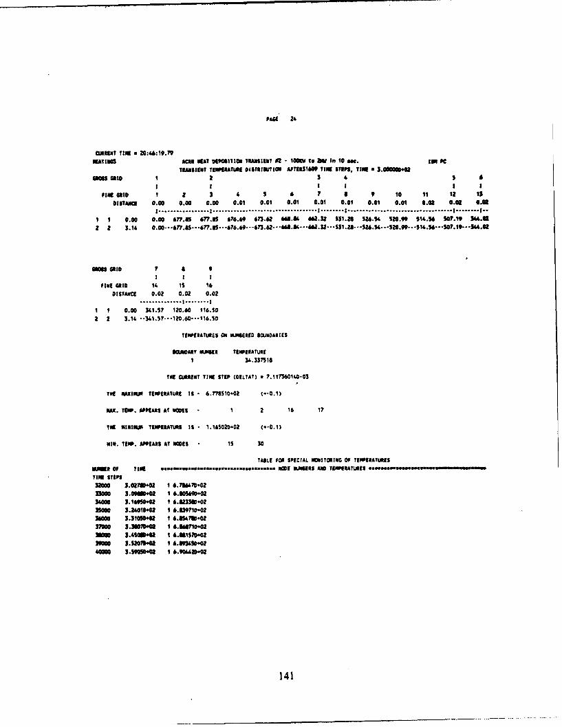
PAGE 2'

ClURRNT TIME u 2:46:19.79NEATINGS ACIN NELAT 04POSITICO TRANSIENT 02 - loOOW tG bW In 10 SMg. Is" PC

TRANSIENT TENPtILATURS OASTRIUUTIO AFTER316011 TIME STEPS, ?INE 3.000000.02GRD¶ 2 3 6 S 6

time (IDI 1 2 3 4 S 6 ? 1 9 10 11 12 isDISTANCE 0.00 0.00 0.00 0.01 0.01 0.01 0.01 0.01 0.01 0.01 0.02 0C0R 0.02

I .. . ..... .. I ... ...... ...... . ...I. ... I .. . .... . ... .. . ... . I ... .. I..

I 1 0.00 0.00 677.891 677.6 676.69 673.62 664.84 662.32 531.261 526.54 S20.99 514.56 SST.19 34.011a 2 3.14 0.00 ..- 7. 6".45 .. 7.85 .. 676.69 --- 673.62 ... 666.16-W66.32 ... 531.28 ...526.S4 ... 520.99 ... S14.56 ..- 0. SO W- 364.02

GRSSID 7 a 91 1 I

fIaE GRID 14 Is 14DISTANCE 0.02 0.02 0.02

........ .... II 1 0.00 341.5? 120.60 116.502 2 3.14 .- 4 .3..-120.60 ... 116.50

TEMPERATUIES ON NII4SEREE SOMNARIES

BOUNDOARY BMUMER TEMPERATURE1 36.337518

THE CURRENT TINE STEP (CELTAT) - ?.im736140.6

THE MAXIMU TEMPERATURE IS 6.77810.IO02 t(*01)

MAX. TEMP. APPEARS AT NODES . 1 2 16 17

INE 0111101111 TEMPERATURE IS 1.16502D.02 0-0.1)

MIN. TE10. APPEARS At UWE$ 1s 30

TAIL[ FOR SPECIAL WONITORING Of TEMPERATURESSlURK OF TINE MOVans.s~se.v...s.s.NE NPJ.SER$ AND TEIPRATRIAS *. .. h. m ~ .

TINE STEPS32000 3.027111102 1 6.736470-0233000 3.090011#02 1 6.8056110#02340001 3.16960*02 1 6.623360.02350M 3.24010.02 1 6.839?10.02360001 3.310501402 1 6.654710.022700 3.380710.02 1 6.161114002360M 3.41000.0 I 6.661578.902"39oll 31.112070402 1 6.693450.0am00 3.59050.02 1 6.904426.02

141

PACE 25

OUIENT TIME * 21: 3:49.31

NEATIND ACII MEAT DPO0SITION TIANSIENT 12 - TOM tO 2" In 10 Oft too PCTRANSIENT TOMNATUsI DISTRIBITION AFTER40136 TINE TEPS. TIRE 3 .590019402

m GRMID 1 2 3 ' S 6I I I I I I

Fin GRID 1 2 3 4 5 6 7 1 9 10 11 It 11DISTAICE 0.00 0.00 0.00 0.01 0.01 0.01 0.01 0.01 0.01 0.01 0.12 0.02 0.02

I ................. I ............................. I . I..................... I ........ I--I 1 0.00 0.00 640.5M 490.59 69.37 &4U.16 661.18 674.39 539.83 534.91 MI9.17 S2.2 514.97 349.342 a 3.14 0.00---.69O.SS ... 6910.39--699.31F--... 6.16---81.181.---674.3---539.83 ... $S4.91--- S29.1?7---S52.SS --- *514.9? .. 349.36

OSS GRI 7 8 9I I I

FINE M1ID 14 15 16OISTAICI 0.02 0.02 0.02

.............. I . ....... Io

I 1 0.00 34.6U 121J.6 1W7.552 2 3.14 --36.2-... 121.76-..117.55

TEMPERATUIRES ON NUSMERED OUtNOARIES

$JOIOANY NIII6ER TIMPERATUIE

I 36.S24961

THE CLORENT TIME STEP (DELTAT) a 6.972291490-03

TiE MARINM TIEP ,RATUEI IS - 6.905U..02 (0-0.1)

MAX. TEMP. APPEARS AT NOES 1 2 16 17

TI MINIMAl TEMPERATUME IS - 1.17S540.02 (0-0.1)

NIN. TEMP. APPEAIS AT NOES 15 30

TASLE FOR SPECIAL MONITORING OF TEMPERATURESNUME OF TIME NOE OMEiNS.w. llll. tllnl.llatlle.1 ... AND TEMPERAT•• fES Ilmtin4m ll.

TIME STEPS

41000 3.6602.02 I 6.914550.0242000 3.79D02 I 6.92390-0243000 3.730002 1 6.932580.0244000 3.LO =0.0 1 6.9405110.024SO00 3. *790.02 1 6.947970.0244000 4.00710.02 1 6.94810402

47000 CO.MMN002 1 6.91130*0249000 4.14S0.O I 6.9449M#02

142

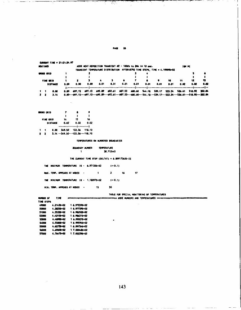
PACE 26

fVAUNT TINE Zi2:21:34.97

NEATINER ACER MEAT DEPOSITION TRANSIENT 92 - IOOKV to 2M inI 10 am. lip PCTRANSIENT TEJEEATIME DISTRIBUTION AFT11487I2 TINE STEPS. TIME *6.19999202*

GRSSID 1 23 4 5I I

FIREGRID 1 2 3 4 7 s 9 Ill II III aDISTAINC 0.00 0.00 0.00 0.01 0.01 0.01 0.01 0.01 0.01 0.01 0.02 0.01 .0.1

I...............I ................................ I..... I............................. I.........I..I1 0.00 0.00 697.13 697.13 695.69 692.61 667.53 610.60 1144.18 S39.17 1133.34 1116.61 S16.92 352.94a a 3.14 00 . .1 . 9.3--6.9..626 . 8.3..64.0..S.8..S91 . n3 . U . 119 . E0

GRS1ID ? a 9I I I

FINE GRID 1/. is 16DISTANCE 0.02 0.02 0.02

.. .. .. .. I. ..... II1 0.00 369.50 122.36 116.10

2 2 3.14 -- 349.50 ... 122.36 ... 1l6.10

TEMPERATURE$ ON WMISSlE BOUNDARIES

BOUNDART IIUER TEWERAYRE1 38. ?1 264

TNE CURRENT TINE STEP (DELTAT) a 6.89917062D-03

7NS NAXIMMJ TINAWIATURE 12 6.971300.02 C-.0.1)

PAX. TE1W. APPEARS AT 11OUE 1 2 16 17

THE NIUUR.UM TEMPERATURE IS 1. 180970*02 0-0.1)

MIN. MOW. APPEARS AT VMS . Is 30

TABLE FOR SPECIAL MONITORING OF TEMPERATURESNMBSER oP TINE OWUU.03U.5..f.uE NUMBRES AND TEMPERATURES ..... u.a.uin .om in

TINE STEPS490010 4.21431102 1 6.973390.02S0a0 4.20330.02 1 6.977390.0211,000 4.3328.02 1 6.912200.0212000 4.421011002 1 6.9610.02O9130111 4.66909.0 1 6.1190270#02560011 4.11695.02 1 6.1939400021SUN 4.62730.02 1 6.991540.021600 4.10600.01 1 1'.00014111021700 4.764710W0 1 7.003390#02

143

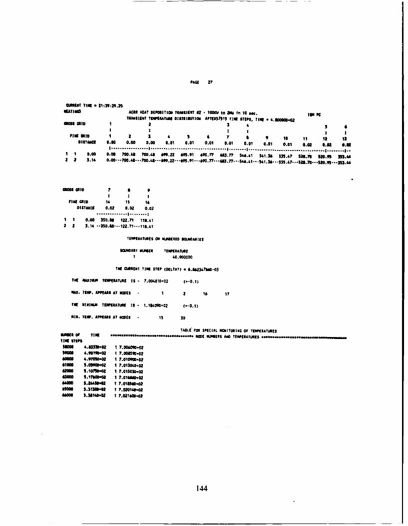
PACE 27

OUNT TIME a 21:39:29.20MEATINO ACAS NEAT DPOSITION TRANSIENT 92 - lOOK to 2M in 10 sec. t PC

TRNBSIENT TE1N01uATM DISTtISUfIOV AFTEI57515 TIME STEPS, TiME a 4.gOO00 *QaOm S IO 1 2 3 4 I 6I Ii I

FIE I1o 1 2 3 4 s 6 1 1 9 10 11 12 1iDISTANCE 0.00 0.00 0.00 0.01 0.01 0.01 0.01 0.01 0.01 0.01 0.02 0.02 8.E2

I ................. I ............................. I . I..................... I ........ I.-1 1 0.00 0.00 700.48 700.48 69.22 69.91 690.77 613.77 S6.41 11.36 35.47 S16.70 520.95 33."62 a 3.14 0.0 48.7M48 92.66".91.690.. 6.7- 6.4-41.36. 3S4?.28 .°2"-S34

I GRlID 7 0 9i I i

FINE GRID 14 1 16DISTANCE 0.02 0.02 0.02

..... "* ....... I ........ I

1 1 0.00 350.U 122.71 118.412 2 3.14 -- 350.-..-122.71--.118.41

TENPERATURES ON ENEEo8 IOOARIES

B5JUOARYT HUEt TEMPERATURE1 60.900000

TIE CUtIIT TIME STEP (OELTAT) - 6.8623476W*03

TNUE MA•lM TEHEERATURE IS .. 004010.02 (--0.1)

MAN. TENP. APP•ARS AT OWES 1 2 16 17

TIE HNIMiU TEIERATLIA IS. 1.184090D02 (.-0.1)

NiH. TEMP. APPEARS AT NOUES Is 30

TAILE FORU SPECIAL MONITORING OF TENPERATURESvim*t o TIN 0001letelisme seals..S s H JMBSERS AND TIMPERATURES ,,o,,-..n,,, .. m.......Titll sit"I

M 4.1330+02 1 7.006090.02"000 4.100190002 1 7.901139042a0 4.97050.02 1 7.010900026100 1.03901002 1 7.013040.0262000 S.10751002 1 7.015030.026300111 5.1760116" 1 7.016W*00266000 5.2660o. 1 7.018600211001 5.31301012 1 7.0201woI.0600 5.36140*02 1 ?.021600.02

144

PAMi 20

aelsmT TiME a 21:57:30.14hATIU|O ACHI NEAT DEPOSITIO TRANSlIE NT - 0I00k to ZIN In 10 la. IM PC

TRNSaIENT TEMPERATU OREIMINUTION AFTERO627I TIN1 STEPS, TIlM * S.3fi9DonamS GR6ID 1 2 3 & 5 6

I I I II I

FIE 01I0 1 2 3 4 S 6 7 a 9 10 II 12 isDISTANCE 0.00 0.00 0.00 0.01 0.01 0.01 0.01 0.01 0.01 0.01 0.02 0.01 0.11

I ................. I ............................. I . I...................... I ........ I..1 1 0.00 0.00 70M.20 702.20 700.93 W7.60 692." 65.40 S47.56 S2.4& 536.5? S9.76 521.90 356.15a a 3.14 0.00 .- 02.. *20 .. 02.20---.00.93 .- 697.60-... 692. -6-5S.40- .• S47.56...542•, ... -536.57---529.76* . *52I. .-354.1S

GOSS GID 7 S 9

1 I I

rIm cIte 14 is 16

OISTANCI 0.0? 0.02 0.02.-............. I ........ I

I 1 0.00 3S1.18 122.06 1183.S2 2 3.14 -- 3513.58--.IZ2.86-...18.S5

TENPERATURES ON WNIIIEN BUIiOUAlRES

mg.UiOAIal UUJIhE ?EWPlUA'UEI

1 60.900000

TNHE CURRNT TINE STEP (OELTAT) v 6.&4AS022ID-03

TMIE MAINA TEMPERATURE ISE - 7.02197D.02 (*-0.i)

MAX. TEN. APPARSI AT UWE - 1 2 16 17

TiE MINIM TEIPEATUIRE IS- 1.1S6530.02 (0-0.1)

MIN. TENP. APPEARS AT NOES - IS 30

TAII.E FOR SPECIAL MONITORING Of TENPEIATUIREUIRW OI TIM I01 NUMBms..ll.lmelllmlllllSERS AND TEIMPBiIRATUEIS

TIME STIPS

67000 5.,4990.02 1 7.02290•.02

""00 5.11630.02 ?. 024200*02

A000 5.3467".0 1 7.02536.02

"7 0 5.6551002 I 7.02443D.0271000 1.721s500 I 7.02742.*02

r2n 5.7I190.0 1 7.020340.0"

73000 5.8603be2 1 ?.0292W0.027400 5.92960001 1 7.029990.027500 5.9900.02W 1 7.03073.02

145

PAGE, 29

CURRET TIlN a 2:15:32.77HIATIUSS ACE NEAT DEPOSITION TIASIENT #2 - 100VW to &W In 10 *a. ION PC

TUONSIET TEIMERATUE ISTIBIUTION AFTER?"", TInE STEPS. TIME 5.9999000•2

e GID0 1 a 3 1 6

I I I I I 3

FINE GID 1 2 3 $ 5 6 7 r 9 10 11 12 1I

DISTANCE 0.00 0.00 0.00 0.01 0.01 0.01 0.01 0.01 0.01 0.01 0.02 0.02 0.0I ................. I ............................. I . I ............................. I ...... I..

I 1 0.00 0.00 703.0 7?03.07 701.61 W1.4A 693.29 616.33 S48.14 S43.05 53?.12 330.31 522.52 354.522 a 3.14 0.00 ... 7?03.0? ... ?03.0?7..--101.81---.698.4?7---693.2 ...--16.23 ... S4.14--..543.0S---53?.1z ... 530.31--*.Sn• a..511--52.

am GRID ? a 9I I I

pINg GID 14 13 16DISTANCE 0.02 0.02 0.02

.......... Io** * | ........ I

I 1 0.00 351.94 122.95 118.63

2 2 3.14 -- 351.94.--122.9.--* 110

TEIMIRATUIES ON NUHOMBRD SO.MOANIS

0OJEARY NUMBER TENPEIATURE1 40.900000

TIe CURRENT TINE STEP (OELTAT) a 6.535099240-03

TME NAXIUM TENPERATUE IS - 7.0307002 (.-0.1)

PAX. TIM. APPIARS AT iODES - 1 2 16 1?

THE NIIIMA TEIPEATUE IS - 1.16260*02 (+*0.1)

NIN. TEMP. APPEARS AT IOES - 15 30

TABLE FOR SPECIAL NOWITIORIG OF TEMPERATURES

MR OF TINE i.li l enS NMI NUMBERS AN TEMPERATURS lui..fl s snnnane

TINK STEPS6000 6.0630.03 1 7.031390.02

T70O0 6.133700021 7.03020.02

7m0O 6.20201002 1 ?.032600002"90110 6.2830002 1 7.03100210000 6.33600,62 7.033640.0261000 6.40700002 1 ?.034100.03am00 6.4753043 1 7.030310.02am000 6.54310.00 1 7.0349J0.02

146

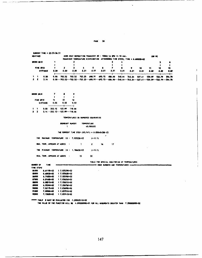
PACE 30

03t3ENT TIME a 22:33:36.51NEATIUS ACRe NEAT OPosITItOl TRANSIENT 62 - 0Od to PRO In 10 Se. is PC

TRANSIEYT TEMPERATURE DISTRIIUTIO AFTEI8326 TIME STEPS, TIME * 6.6000.ooGlID 1 2 3 4. 6

I I I I I iFINE 411 1 2 3 4 $ 6 7 a 9 10 11 12 13

DISTANCE 0.00 0.00 0.00 0.01 0.01 0.01 0.01 0.01 0.01 0.01 0.02 0.02 0.0I ................. I ............................. I . I..................... I ........ I.-

I 1 0.00 0.00 703.12 703.32 702.21 69-.91 693.72 686.66 U48.4 U43.34 117.41 530.19 52.70 354.702 2 3.14 0.00 . 70332 -- 703.52-.- 702.25 - 648.91 .69.72 -- 686.- - •4. - 43.36 ... 53V.41...$S0.59---. 5. I..]35.79

a0mS on 7 8 9S I I

FlUE•l 6 14 1 16

DISTANCE 0.02 0.02 0.02

"°°"** ..... I .... Io*..... I

I 1 0.00 352.12 122.99 116.66

a 2 3.14 -- $52.12-..122.99.-.11.66

TEMPERATURES ON NIUMERERE SCUNARIES

USJSCOARY 1I011t TEMPERATURE

1 40.900000

TIE CURRENT TIME STEP (DELTAT) - 6.830404310-03

TME NAXZIU TEMIPEATURE IS- 7.035230.02 C.-0.1)

MAN. TEMP. APPEARS AT OWES - I 2 16 17

THE NMNIMUM TEMPERATURE IS - 1.186630-02 C(-0.1)

PIM. TEMP. APPEARS AT NOES s1 30

TABLE FOR SPECIAL MONITORING OF TENPERATUSESNUMBER OF TIME NeMIsaeeme . .s ... se m ses. NUMBERhS AND TEMPERATUIES *•m............. ....

TIME STEPS

64000 6.61190.02 1 7.035290,02am100 6.610O2D. 1 7.03163002am 6.74110.02 I 7.03SO9*0287000 6.8160#02 1 7.036&10O2amO 6.11110.2 O• 7.036510.0209000 6.95340*02 1 7.03710.02"mOO 7.021703 I 7.0369*.02"9100 7.0000*02 1 7.037210*02

9200 7.I]63.02 1 7.037410.02

STAILS OUST IS EVALUATED FOR 7.20002110*02TUE VALUE OF TI FUNCTION WILL IS 4.090000000.01 FOR ALL ARIGUMNTS GREATES TIN" 7.200000000*02

147

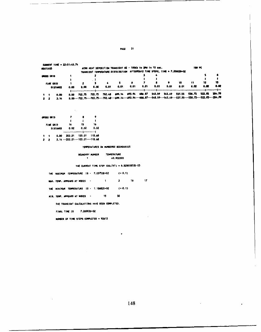
PAGE 31

OU1111T TIME 22:51:40.74NKATIINGS ACNE NEAT DEPOSITION TRANSIENT 62 - O to Kn 10 2Wcf i W.

TRANSIENT TINKEItATUWI ISTIUTIgllM AFTIEI 12 TIN[ STEPS, TIlE 7.20000.

Sa Clio 1 2 3 ' S 6

1 . I I I I

FINI GRI 1 2 3 4 S 6 7 1 9 10 11 12 i3

DISTANCE 0.00 0.00 0.00 0.01 0.01 0.01 0.01 0.01 0.01 0.01 0.02 O.0 *.I ................. I ............................. I . I..................... I ........ I..

1 0.00 0.00 703.75 703.7•5 02.48 699.14 693.94 686.87 548.59 S43.49 S$7.SS SM.13 S.q9 34 .19

2 2 3.16 0.00... ?03 ?S. ... ... 048.6". 14..69394 .. 68.87? .. %8.59 543.49 5137.55 ... 530.73 -. 22.9•- -.-3S4.7W

006 3I10 7 8 9

I 1 IFIE GRID 14 15 16

DISTANCE 0.02 0.02 0.02

0..o...o*o ....- 1-. ...... I

1 0.00 352.21 123.01 118.66

2 2 3.14 -. 352.21---.123.01-... 118.68

TI4PIOATURES ON MIJISEM1R40I iOARIES

BOUNOARY NIIBEE TENPERATUIE1 &0.900000

THE *JIRtENT TIRE. I touvhl TE.¶~ * .1280020*03

T'OE 0AXIZM TEMPI[ATUlti IS- 7.037320#02 (0-0.1)

N•a. TEMP. APPEiARS AT M1OVES 1 2 16 17

TOE INIMUM TEIMERATUIE IS- 1.1868=002 (.-0.1)

NIN. TI[P. APPEARS AT iNMI$ 15 30

THE TRANSIENT CALCULATIONIS NAVE IEN EOMiPLETED.

FINAL TIME 13 7.200030-02

SIEIu Of TIME STEPS ComxTIo - 92612

148

PAGE 32BEIN TIE STUDTY SATE CALOAMIONI$SUSl OF IXTRAPOLATIONITERATIONS mUea U 0001 TI'IlEATWE FACTOR

149

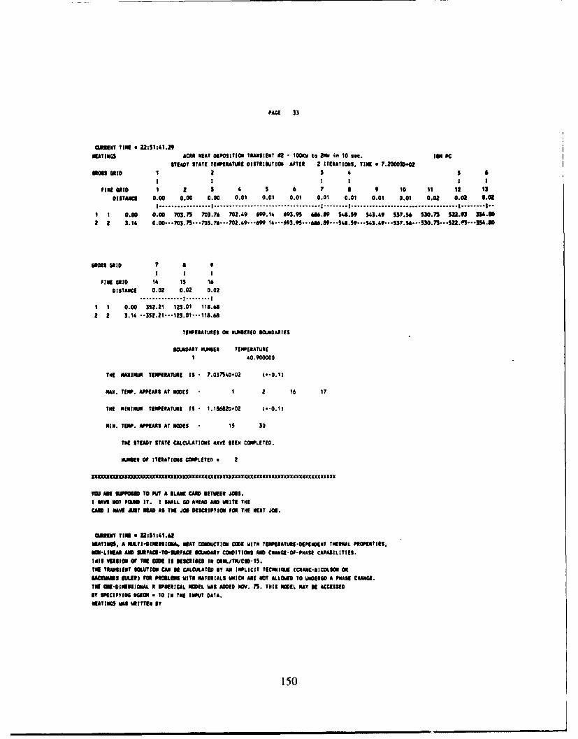
PAGE 33

CURRENT TIME 22:51:41.29NEATINlS ACM NEAT DEPOSITION TRANSIENT 82 - lOO9d to 201 in 10 see. IN PC

STEADY STATE TEMPERATURE DITIISIUTION AFT[* Z ITERATIONS, TIME T.200030.0ClioS 1 2 3 4 5 6

I I I I I IFINE MID 1 2 5 4 5 6 7 I 9 10 I 12 13

DISTANCE 0.00 0.00 0.00 0.01 0.01 0.01 0.01 0.01 0.01 0.01 0.02 0.02 L.aI .............. I ............................. I . I..................... I ........ I..

I I 0.00 0.00 703.J5 703.74 702.49 699.14 693.95 646.89 S8.S9 $.3.49 537.56 530.73 12.93 314.812 2 3.14 0.0- ... 3--- m.r6---. n2.49---699 % -- 693.9---686.89---. 5.59---S63.49--537.56---530.73-*-. .•--*•.80

GRS GRID 7 1 9I I I

FINE GRID 14 Is 16DISTANCE 0.02 0.02 0.02

* . ... .. * * * . . . . I- .. . . . . . I

1 1 0.00 352.21 123.01 116.68

2 2 3.14 -- 3522.1--- 123.01--- 1186.

TEMPERATURES ON hIUMERED BOUJNDARIES

BOUNDARY "IWIE TEMPERATURE1 40.900000

TIE MAXIMO TEMPERATURE IS 7.037540-02 (--0.1)

PAX. TEMP. APPEARS AT OWES 1 2 16 17

TNIE INIMUM TEMPERATURE IS 1.1868M-02 (0*0.1)

MIN. TE•P. APPEARS AT NUES 15 30

TIE STEADY STATE CALCULATIONS NAVE SEEN COMPLETED.

NUMIER OF ITERATIONS COMPLETED - 2

XXXXXXuXXXCIXXROIxDXXXXKXXXX)vxxKXXXXXXXXXKXXXXXXXXKXXXXRXXXXXXXXXXXX

YOU AE OUPPOSE TO PUT A $LAN CARD GETITEN JOBS.I MOVE NO? POUAD IT. 1 SWALL 0O ANEAD ANDWI TEtNSCARD I NAVS .UST ItAD AS TNE JOB DESCRIPTION FOR TIE NEXT JOB.

CUtINT TINE e 22:11:41.62AItTIN6, A ELTI-OIIEIIOEA. NEAT CEISUCTION MDE WITN TINPI[ATUIt-OEEPENT T[ERMAL PROPERTIES.

1011-LII1M AND SUNIFACI-TO-UPACE BIOUDARY CONDITIONS AND CNANGE-OF-PKASE CAPABILITIES.

111 VERSION OF tIE! IE DESCRIBED In ORtL/TN/CID-15.TI TRIRIINIT SOUTIf1 CAN BE CALCULATED Bt An IMPLICIT TICHNIQUE (CRANZ-NICOLSON 0i

UACEWR OU[R) PU PIKEINS WITN NATERIALS UWICN ARE NOT ALLOlWD TO UNDERGO A PNASE CNANGE.Tit Oil-DIEMSIOALM I PI[ERICAL MODEL WAS ADDED NOV. 75. TNIS NOIL NAY IS ACCESSEDIT SPECIFYING INOEU a 10 IN TIE INPUT DATA.NEATIWGS lt UITTIEM BT

150

PAGE I

mU~y TIN a 14:35:22.61 DATE :9/16/1992EATIESS. A MAT I-DIMENSIONAL NEAT CONDUCTION CODE WITH TIMPINATU.WE-0111NDENT TIMIRMAL PROPERTIES,

NS1LIMEAA ANS PAPACE.TO*MFACE BOUNARY CONDITIONS AND CMANGE*O9*PHASE CAPABILITIES.THIS VINSPSN OF I CODE 1S DESCIsED Is SNML/T0/CUIS-.INE TRANSIENT SOLUTION CAN If CALCULATED IT AN IMPLICIT TECNIUIS CCRANX-0IULIO 01

hACIOMS SUNt) FOR PROLMN WIll NATIPALS 1111W ORf NO? ALLOWED 10 UNDERkGO A PUNS CHANGE.YME =-IM.ENSIONAL I OPMNEICAL MOEL WAS A0010 NOV. 75. TNIS MOL MAT BE ACCESSED

By SPICIFYPMINEO a65 10 19IN[ THEPNM DATA.E9ATINOS WAS WITTEN ST

M.D. iTURNERD.C. BLUE)3.3. SlUAN-TOW

camTel SCIENCS DIVISIONUIOPS CASPID CORPORATION, MACLIAN DIVISION

OAK RIDGE, TENNESSEE 37830

THIS VERISPN OF HEIATING CAN HANDLE A NAXIMUM Of 400 LATTICE POINTS.

IPUM.T RETURN

JO DESCRIPTIOH� ACER NEAT DEPOSITION TRANSIENT 41 60 MOO p uhSa - 13 mon width 8 half

6105111Y TYPE wiIER 2 (OR ITINUMER OF 118155w a

NUMER OF MATERIALS &ASlOF HEAT GENERATION FUNCTIONS I

WJSR OF PIPITIAL TEMPERATURE FUNCTIONS INUMBER OF DIFFERENT KINDS OF BOUNDARIES 1TIPS PROBLEM NVOLVEVS TENIFIIATURIE-DEPENOEN'I PROPERTIES.

NUM101 OFPOINTSPIN I m X 0 1LATTICE 9NUMBER OF POINTS PH GROSS 1 0R THETA LATTICE 2MISE& Of POINTS IN GROSS Z LATTICE 0NOUNR OU ANALYTIC FUNCTIONS I

WiSER OF TAULN" FUNCTIONS aNUMSER Of TRANSIENT PRINTOUTS SPECIFIED S

TEMPERATURES OF SELECTED NMI$ WILL BE MONITORED EVERY 1000 ITERATIONS OR TINE STEPS.

PROBLEM TYPE BUISER 3STEADY STATE CONVERGENCE CRITERION 1.00000000-05MAXIMUM NUMSER OF STEADY-STATE ITERATIONS ION0WWISE OF ITERATIONS BETW.EEN TEMPERATURE DEPENDENTPAANETES EVALUATIONS FOR STEADY STATE CALCULATIONS aINITIAL OVERIELAJIATIOH FACTOR (BETA) FOR STEADY STATE CALCULATIONS 1.90000000TIEI PIMMIENET 1.00000000-03LEVYS EXPLICIT 101T111 WILL BE USED WITH A 11IE STEP 1 TIMESLARGER THANI THAT USED IN THE STANDARD TRANSIENT TECNNIOUR.INITIAL TINE S.0000OOD-010

FINAL TIME 2.00000D.01#0

151

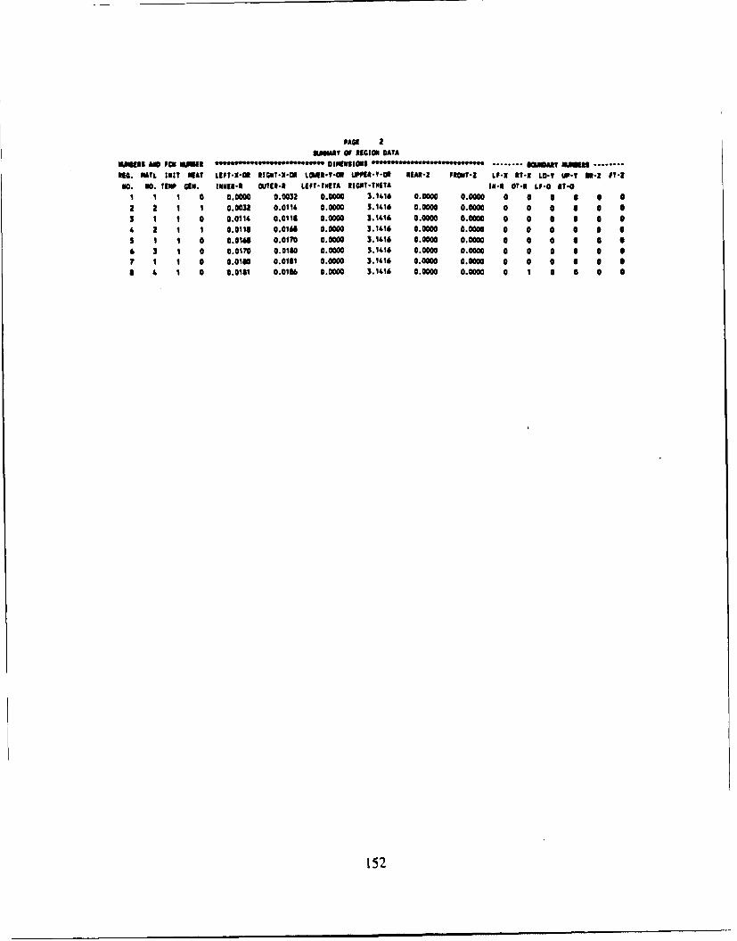
PACE 2kSMET OF REGION DATA

1011a$a AN PCs amulR DO~ ~ ' IMENSIONS .'*~ ..... inGagaa mamaNOC. WATL IURT NEAT LEFT-N-U *1 IGNT-1NU LOUN-V-0E UPPSA-T-0El IS*AZ FhUT, LI-N IT-N L0-V ip*v M*Z fT*2

No. 0O. low GEN. SuBI-1 OlJT-*l LEFT- TOETA RIGIIT-TNETA IN-rn 01.1 LI-O IT-0S I I a 0.0000 0.0032 0.0000 3.1416 0.0000 0.0000 0 0 0 0 6 02 2 1 1 0.0032 0.0114 0.0000 3.1416 0.0000 0.0000 0 0 0 0 6 0

3 1 1 0 0.0114 0.0114 0.0000 3.1416 0.0000 0.0000 0 0 0 0 a/. 1 1 0.0118 0.0166 0.0000 3.1416 0.0000 0.0000 0 0 0 * * *5 1 1 0 0.0166 0.0170 0.0000 3.1416 0.0000 0.0000 0 0 a a * *6 3 I 0 0.0170 0.0180 0.0000 3.1416 0.0000 0.0000 0 0 0 0 07 1 1 0 0.01W0 0.0181 0.0000 3.1416 0.0000 0.0000 0 0 0 0 0 *a 4 1 0 0.0161 0.0166 0.0000 3.1416 0.0000 0.0000 0 1 0 0 0 0

152

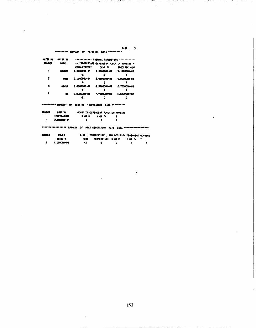
PAUI I

SUMPIAIY OF MATEI|AL DATA

MTIERIAL SMTIEIAL ............ TNERMAL PAIDT90S ............NmiUER UM -- TIEPERATUtE-KPENqUOT FUNCTION M OItS .R

COmiUCTIVITY DENSITY SPECIFIC NEATNIVOID 0.00G000-01 OQOOOOW 0-O S 9IZM0 03

".6 -? 0

FIEL 2.4000C.0t1 3.SSO .00003 0.O0oc0oa-0o0 0 .1

(Ua= O.OOOWOM-01 8.S7000mDosu 2.lOOOOOD.O.5 0 0

4 S 0.0000000*01 ?.950000D.0.3 5.O200=-02.2 0 0

MIUMRtY OF INITIAL TEMERATURE DATA - *-e

NMISR INITIAL POSITIUN-0PI[NOENT FUNCTION iUM[tS

TEIMPRATUIE x n It T OR NN 21 2.UOOOD.0I 0 0 0

eeoee~eoe M NIARY OF NEAT GIENEIATION RATE DATA ****e **'

MIUNSE POWER TINE*, TEMPERATURE-, AND POSITION-DEPENODET MUNSERS

DENSITY TINE TEMPERATURE X OR 1 Y Olt TN Z1 1.000000.00 -3 0 -4 0 0

153

..... EVERAL.... 131Wh3AlUZt-................................. WAY TRANSIER COEFFICIENS.........................INFUMATION RELATED FUNCTION HMamS

0O. TYPE FC? hRIMPS lAURE FORCOW001. RADIATION VATUML CO MIOMENT FLUMFLAG & TINE FCT ASSOC.

FCTS

1 1 2 1.0000000.00 1.000000440 OOO~c-O 0.0000 -01 0.000000-Ol 00 000S 0.000000-01it~lE 0 0 a 0 0TIP 1 0 000

GROSS LATTICES AM MUNANE OF ImcIalmwTs

0.000000 0.003160 0.0111.30 0.011810 0.016760 0.0156%7 0.017963 0.01861110.018610

THETA am Y0.000000 3.11.1593

LIST1VG OF ANALYTIC FUNCTIONS

F(V). AMI # A(2)*v # A(S)*r*2 - AC.)*COS(A(S)*V) - AC6)*EXP(A(?)*V) * AMIS)SN(A(9)V) - AC10)IL06(AC1I)V

NO0. AMt AMt AMS AM. AMS AMS AM? MES) AM9 ACIO) AC11)1 0.0000-01 1.0000.000 2.796-01 0.0000-01 0.0000-01 0.0000-01 0.0000-01 0.0000-01 0.0000-01 0.0000-01 0.0.OO1-O

154

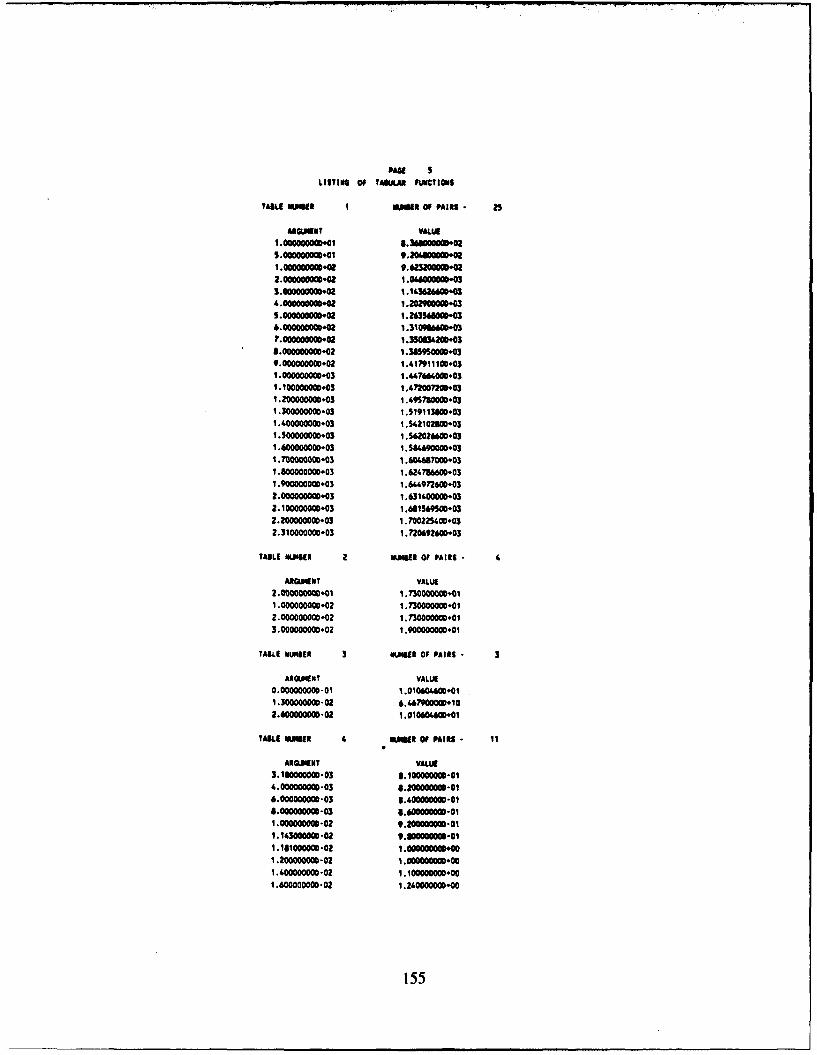
PAGE 5LISTINGOF0 TAIUA FUNCTION$

TABLE U.JEB I NSAI OF PAIRS- 2

ARGUMENTVALUE1.000000000.01 6.366000000.025.ooooooo00oi 9.2040m000.01.0000000011+02 9.6232000m0.02.000000000+02 1.066000000.033.000000000.02 1. 143626600.036.000000000.02 1.202900000.05.000000000.02 1.263%680040.&.000000000402 1.31090060D.031.000000000.02 1.350834200#032.000000000-02 1.365950000039-000000000.02 1.4t7911100.031.000000000.03 1.447664000+031.100000000.03 1 .47120072004031.200000000.03 1.495750000#031.300000000.03 1.519113800-031.400000000.03 1.S42102600.03I .500o00oo040s i .5626600.031.600000000.03 1.58W69000003lJ.7000000.03 i.6041.667000.031 .800000000.03 1.624736600.031 .900000000.03 1 .644972600.032.000000000.03 1.631400000.032.100000000.03 1.681569S00.03

2.200000000.03 I .702251.00.032.310000000.03 I.720692600-03

TABLE NUMBER 2 NUMBER 0F PAIRS

ARGUMENT VALUE2.000000000.01 1.730000000.011.000000000.02 1.730000000.012.000000000-02 1.73000000013.000000000.02 1.900000000.01

TABLE KOBIE* 3 NLUMER OF PAIRS - 3

ARGUMENT VALUE0.000000000.01 1.01060"600#011.300000000-02 6.467900000.102.6000000011-02 1.010601.600.01

TABLE ULMER I. WULER OFPAIRS - 11

AROUMEIT VALUE3.160000000-03 6.100000000-014.000000000-03 6.300000000-016.000000000-03 6.400000000-01S-00000000-03 8.600000000-011.000000000-02 9.900000000-Ol1.143000000-02 9.600000000-011.161000000-02 1.000000000.01.200000000-02 1.000000000-001.400000000-02 1.100000000.0001.600000000-02 1.240000000.00

155

1.70Maoooo0o i.aa0oocm*oo

156

PAU 6

LAROUNEN VALUE0.000000000-01 5.230000000.011.000000000.02 S.'AOOOOsos.l2.000000000*02 5.650000000.0S.000000000-02 S.SIOO~oO.i4.000000000.02 6.070000000.011 .0OOO0OOOD.03 7.2700000m00.1

TABLE ULER 6 OiN.ISIOF PAIRSS - 1I

mommyM VAILUE2.000000000401 7.200000000-02I .000000000402 7.200000000-022.0000000O0.02 1.150000000-o¶3.000000000.02 ¶ .510000000.014.00000000002 l.640000000-015.0 O00o000.oa0 2.1300000m0-016.000000000-02 2.500000000-017.000000000.02 2.70000000-01G.OOOOoOOOWOoz 3.040000000-019.000000000.02 3-300000000 -011.000000000.03 3.540000000.oi1.200000 000.403 4.050000000-041.400000000.03 4.5s000m000.1-.600000000403 SIOZODOOOOD-041.800000000.03 5,430000000-042.000000000.03 S,790000000-012.500000000.03 6370000000-013.000000000-03 7,450000000-01

TABLE UMD~ER 7 SEE OF PAIRS - 3

ARGNOIEM VALUE2.000000000.01 3.292800000-oi1 .200000000.03 1.63340000-012.600000000.03 1.673320000-01

TABLE NUMSER a NUMBER OF PAIRS - 2

AGiqwiv VALUE0.000000000-01 2.000000000.011.000000000.01 2.000000000*01

TAKLE OF OUTPUT TIMIE

OUTPUT OUTPUT OUTPUT OUTPUT OUTPUT OUTPUT OUTPUT OUTPUTno. TIME NO. TIME 30. TIME 30. TIME1 0.000000-01

a 1.300000-023 2.6000011-026 3.000=0-025 1.000000.016 9.000000-01

t7 1.000000.0

157

U M11TWMS OF tIN FOLLOWUIG MKS5 WILL U NMOITOUE

gVST 1000 IlBATIS ON1 1fix[ UTPS.

158

I15

159

PAGE a

FIN LATTICE, X 0l . 1 0 TVETA, ANS Z

2 0.001590 3 0.003160 4 0.0021242 S O.M03 0.00036?

7 O.Ot11so a 0,011810 9 0.013018 10 0.01o u I1 O.01"SS

1i 0.010760 13 0.016967 1¶ 0.0173 Is 0.01010m 16 0.018i10

1 0.000000 2 3.141593

TMS PROBLEM CONTAINS 30 UOES.

** TABLE 6 MIST ME EVALUATED FOR 2.000000000001

Til VALUE OF TNE FUNCTION WILL B 7.200000001-02 FOR ALL ARGUMENTS LESS TRAM 2.00000000.-01

*** TAILE 2 MST EVALUATED FOR 2.00000000001

THE VALUE OF THE FUNCTION WILL BE 1.7110000000.01 FOR ALL ARGUMENTS LESS THAN 2.000000005.01

' TAILE ? MUST MI EVALUATED FOR 2.000000000-01

THE VALUE Of T•E FUNCTION WILL KE 3.22800000-01 FOR ALL ARGOMEUTS LESS THAM 2.000000000-01

160

PAGlE 9SM~ILIIY CRITERION FOi lO0 NMI

I .3202 2 2.28990.81 3 2.45480.0 1. 2.67600-01 5 2.OSSIol 6 I.7721S-O17 977-2 8 9.70570-02 9 9.7073-02 10 9.708311-02 11 0.71100-02 12 2.132110-02

13 2.1823-02 11. 3.11810-02 15 3.24M99-02 16 3.732-02 I7 2.239-01 1Is 54OI9 2.676110-01 20 2.1530.01 21 2.7721001 22 9.37870-42 23 9.70570.02 at. 9.NM2-ozas 9.70m3-02 26 9.714.0D-02 2? 2.13M-2w l 28 2.1823-02 29 3.11800-02 so 3.21.91-4

Till STABILITY CRITERlION 15 2.13287190-02 FOR POINT 12

INE IUUT TIME INCREMENT SATISFIES TilE STASILITI CRITERION.

161

PAGE 10

C08*1T 111T a 14:35:24.73IIATINgS ACRA NEAT DEPOSITION TRAUSIENT 61 - 6400 Ol pulse 13 ine widtII 0 hl0tf IBM PC

oAP OF THE NM0 MImUIES

m GRDa 1 2 A 6 S 0I I I ! ! I

pl16€t0 1 2 3 4 S 4 7 8 9 10 11 12 1310STAsc€ 0.00 0.00 0.00 0.01 0.01 0.01 0.01 0.01 0.01 0.01 0.02 0.02 .IM

I ................. 1- ................................ I ........ I ................................... I ........ I..

I 1 0.00 0o 1 25 3 4 S 61 71 a 9 10 111 1212 2 3.14 01 ...... 16 ....... 171 ....... ig .19...... 20 ...... ?211 ...... 1 ...... 23 ....... 24 ....... as ....... 261 ...... n-*

amS Cio 7 a 9

FlUE GRI0 1 s 1S 16

DISTANCE 0.02 0.02 0.02S.............. I °... .... I

1 1 0.00 135 141 1552 2 3.14 "--281 ...... 291 ...... 301

162

PAGEI 11

CUI01uT t 14:35:T5.2MNIATINO AMII NEAT DIPOSITION TRANSIENT #1 6400 m polut o 13 not widith haLf IN PC

STEADY STATE TEIPEIATUIR DISTNIOIIUTI0 AFTER 0 ITERATIONS, TINE 0 0.00000-01

GRIUDt 1 2 3 6I I I II I

FIN in 0 1 3 3 4 S 6 7 a 9 10 11 12 13

01DSTNCE 0.00 0.00 0.00 0.01 0.01 0.01 0.01 0.01 0.01 0.01 0.02 0.02 0102I ................. I ................................... I ........ I ................................... I ........ I..

I 1 0.00 0.00 20.00 20.00 20.00 20.00 20.00 20.00 20.00 20.00 20.00 20.00 20.00 3.60

2 a 3.14 0.00 .... 20.00 .... 20.00 .... 20.00 .... 20.00 .... 20.00 .... 20.00 .... 20.00 .... 20.00 .. 20.00 .... 20.00 .... 20.00 .... .00

GROSS Gild 7 8 9I I I

FINE GRID 14 1i 16

DISTANCE 0.02 0.02 0.02........ •...... I ........ I

I 1 0.00 20.00 20.00 20.00

2 2 3.14 --- 20.00 .... 20.00 .... 20.00

TENPERATUNES ON MMIURlD SJNOAtNIES

iQOIOAT 001614 1EMNPERATUIE

1 20.000000

Ti MAXIMAU TEIPRATURE IS" 2.00000O001 (4-0.1)

mAx. TENP. APPEARS AT N0O1 - 1 2 3 5

6 7 a 9 10

11 12 13 14 1s16 17 1s 19 2021 22 23 24 2526 2? 28 29 30

TIlE ,J TEIOPERATURt 13 . 2.0000.01 (--0.1)

Pin. TEMP. APPEARS AT K3DI1 - 1 2 3 4 5

6 7 a 9 1011 12 13 14 1516 17 1 19 20

21 22 23 24 2526 2? 28 29 30

163

PAU 121MII TI STEADY STATE CALCLATIONS

OUNlCS OF EXTRAPIOATIONITERUT IONS oftwidUC( "m TIwISATUEL FAVOR

164

PAW 13

CURRENT TIME 14:3S:25.74INIATIOW ACIR NEAT DEPOSITION TRANSIENT Sl - M00 MW Put" - 13 wge width @ half Ion PC

STRAD1 STATE TENPERATUIE DISTRIUTIOU AFTER 2 ITRATImoOS. TIME - 0.OO oiO*OIOSS GID 1 2 3 4 $ 6

I I I I |

Fin GRID 1 2 3 4 5 6 ? 1 9 10 I I& 1sDISTANMCE 0.00 0.00 0.00 0.01 0.01 0.01 0.01 0.01 0.01 0.01 0.02 0.02 6.02

I ................. I ................................... I . I..................... I ........ I..1 0.00 0.00 20.00 20.00 20.00 20.00 20.00 20.00 20.00 20.00 20.00 20.00 20.00 20.U

2 2 3.14 0.00 .... 20.00 .... 20.00 .... 20.00 .... 20.00 .... 20. .0 .... 20.00 .... 20.00 .... 20 0..--000 .... 20.00 ... 20.00 .... u00

mausIO 7 a 9I I I

FINE GRlI 14 1 16DISTANCE 0.02 0.02 0.02

.............. I ........ II 1 0.00 20.00 20.00 20.002 2 1.14 --- 20.00 .... 20.00 .... 20.00

TEMPERATURES ON NIUMBERED BOUNDARIES

JNOART Y NUMBER TEMPERATURE

1 20.000000

TH[E AZIAUM TEMPERATURE IS . 2.000000-01 (C-0.1)

MAX. TEMP. APPEARS AT NODES 1 2 3 4 5

6 7 a 9 1011 12 13 14 1516 17 16 19 2021 22 23 24 2526 27 28 29 30

TIE MINIiMU TEMPERATURE IS 2.000000D01 (.-0.1)

1IN. TEM. APPEARS AT MDES 1 2 3 4 5

6 7 a 9 1011 12 13 14 1516 1? 1 19 2021 22 23 24 2326 27 21 29 30

TiE STEADY STATE CALCULATIONS RAVIE BEEM COIPUI.TE.

KlOES OF ITERATIONS CMPLETED * 2

165

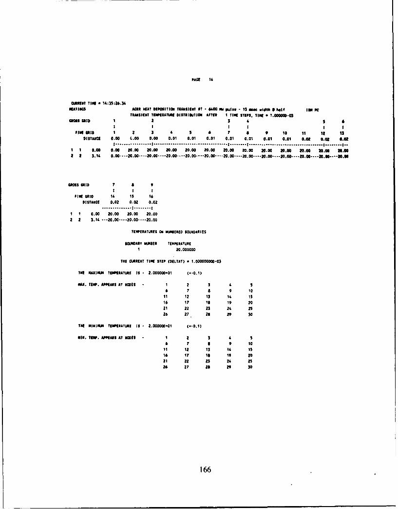
PAGE 16

VANXlI TIN s 14:35:26.34

REATINOS ACES MEAT DEPOSITION TRANSIEET e1 - 600 MW pUtse -S m141e uidth S hllf IN PC

TRAASIENT TEMPERATURE OISTRIBUTION AFTER I TIMI STEPS, TIME a 1.0000W-03;im s ONTO 2 3 5 6

I I I II

FlIo GID 1 2 3 4 5 6 7 8 9 10 11 12 13

DISTANCE 0.00 L.00 0.00 0.01 0.01 0.01 0.01 0.01 0.01 0.01 0.02 0.02 0.0ZI ................. I........... ............... I ........................ I ........ I..

I 0.00 0.00 20.00 20.00 20.00 20.00 20.00 20.00 20.00 20.00 20.00 20.00 20.00 1.01

a 2 3.16 0.00 .... 20.00 .... 20.00 .... 20.00 . ... 20.00 .... 20.00 .... 20.00 .. 20.00 ... 20.00 .... 20.00 .... 2 0.00 .... 20.00-b...0.00

GROSS 0 ID 7 a 9

! I 1

FINE GlI0 16 IS 16

DISTANCE 0.02 0.02 0.02..... . ..... I ........ I

I 1 0.00 20.00 20.00 20.00

2 2 3.16 .-- 20.00 .... 20.O 0 .... O.2O0

TEMPERATURES ON NMOEBEED BOUNDARIES

IRARYT NUMIER TEMPERATURE1 20,000000

THE CURRENT TIME STEP (DILTA?) - 1.000000000-03

THE MAXIU TEMPIERATURI•1 - 2.000000D01 (.-0.1)

MAX. TEIW. APPEARS AT ROES 1 2 3 6 s

6 7 8 9 1011 12 13 16 Is16 17 18 19 20

21 22 23 26 25

26 27 28 29 30

T[E INIMUM TEMPERATURE IS - 2.000000.01 C.-0.1)

NIN. TEN. APPEAIS AT UWES 1 2 64 s

6 7 a 9 1011 12 13 14 IS

16 1? Is 19 20

21 22 23 24 25

26 27 20 29 30

166

PAUE Is

CURRENT TINE * 14:35:28.16NWATINGS ACRE NEAT DEPOSITION TRAISIENT 91 - 6 M Iluts@ - 13 Was uidth 8 helf Ilo PC

TRANSIENT TEIPERATURE DISTRIBUTION AFTER 13 TINE STEPS. TINE 0 1.300000-02

aSm GID I 3 4 $ 6I I I I I

FIUN I I 2 3 4 5 6 7 i 9 10 11 12 13DISTANCE 0.00 0.00 0.00 0.01 0.01 0.01 0.01 0.01 0.01 0.01 0.02 0.01 0.0

I ................. I ............................. I . I..................... I ........ I..1 1 0.00 0.00 27.42 115.82 118.3% 120.70 126.09 134,.79 137.31 142.99 150A.$ 159.87 1663.13 MI.S

2 2 3.14 0.00 .... 27.62. S.112..11. 120.0..12609..1 79...1.1.14239.1..1 159.07 .. 16633 .... 20.15

GMtS GID 7 8 9I I I

FIlE GRID 16 15 16

DISTANCE 0.02 0.02 0.02

* .... o ........ I ........ I

I 1 0.00 20.02 20.00 20.00

2 2 3.14 --- 20.02 .... 20.00 .... 20.00

TENPERATURES ON NJIERED IJUIOARIES

SBUNDARY NiUMER TIEPERATURE

1 20.000000

THE CURRENT TINE STEP (DELTAI) a 1.000000000-03

THE MAXIMU TENPIRATURE IS- 1.635300-02 (0-0.1)

NAX. TEIP. APPEARS AT NONlS - 11 26

THE NININU TENPEATUIRE IS - 2.001620.01 (*-0.1)

NHI. TEMP. APPIEAS AT NOIES 13 14 Is 28 29

30

167

PAGE 16

CURRENT TIlE u 14:35:29.97

ISATINGS ACIIRI NAT ODEOSITION TRANSIENT 01 - 00 MW PuISS - 13 m ,Idth I half ISm PC

TRANSIENT TEMPERATURE DISTRIlUTIOR AFTER 26 TIME STEPS, TIME s 2.60O0m.02

am onto 1 2 3 ' S 6I I I I

FINES ID I a 3 4 5 J 7 A 9 10 11 12 is

DISTANCE 0.06 0.00 0.00 0.01 0.01 0.01 0.01 0.01 0.01 0.01 0.02 O.0 0.01I ................. I ................................... I . ................................... I ........ I.-

I 1 0.00 0.00 71.40 217.06 222.7 227.47 2.13 25..67 260.71 271.16 2." 303.56 31S.02 21.062 2 3.14 0.00 .... ?1.40 --- 217."*--22. •--..227.4?" ... 2813 ... V1.67' ... 71 2J ... 271.16**... M.9-30.36*.. 15.02 .... 21.0

OSS RID0 7 a 9

I I I

FINE ON0 14 Is 16

DISTANCE 0.02 0.02 0.02S...... - .. . I ........ I

I 1 0.00 20.26 20.00 20.00

2 2 3.14 --. 26 .... .2000 .... 20.00

TEMPERATURES ON NIJSERED SOUNDARIES

S0MARYT NUMBER TEMPERATURE1 20.000000

THE CURRENT TIME STEP (OILTAT) - 1.000000=-03

THE PANlMU TEMPERATURE IS - 3.1S0160.02 (*-0.1)

NAX. TMP. APPEARS AT U0011 11 26

TE MINIMUM TEMPERATUJRE 5 - 2.O0D#01 (0-0.1)

MIN. TEMP. APPEARS AT NODES 14 1s 29 30

TASLE 3 MTST RE EVALUATEO FOR 2.600000000-02

THE VALUE OF THE FUiNCTION ILL At 1.010604600.01 FOR ALL ARIGIUENTS GREATER TUAN 2.600000000-02

168

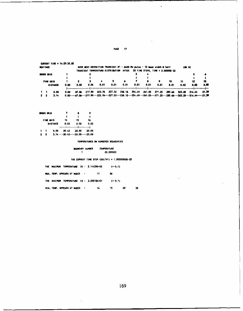
PAUE 17

EI[ENT TIN * 14:35.30.SSNEATINGS ACES NEAT OEPOSITION TRAISIENT 01 - 6400 NW IAute - 15 • ulciw i hatf io PC

TRANSIENT TEEIATUIE DISTIIIUTION AFTER 30 TINE STEPS, TIME a 3.000001-02

GROSS GR0 1 2 3 1 S 6a I I I I I

FINMEGID 1 2 3 4 5 6 7 1 9 10 11 12 aDISTANCE 0.00 0.00 0.00 0.01 0.01 0.01 0.01 0.01 0.01 0.01 0.02 0.02 4.1

I ................. I ............................. I . I..................... I ........ I--I 1 0.00 0.00 0P.M 217.90 222.76 227.52 238.18 2S4.49 261.05 271.25 285.46 303.21 314.44 21.39

S2 a .14 0.00 .... O0.86---.217.90*--... 72.6---227.2..5 2--.•13...--2S4.49---. 61.05---.271.2S---.8M.."---303.28---.314."--...21.39

mosS m=i 7 a 9

FINE GRID 14 15 16DISTANCE 0.02 0.02 0.02

"*... * ...... I ........ II 1 0.00 20.42 20.00 20.00

2 2 3.14 -.- 20.42 .... 20.00 .... 20.00

TEMPERATURES ON NUMSERED SOUNDARIES

C)UNOATY .NUMBER TEMPERATURE

1 20.000000

TNE CUARENT TINE STEP COELTAT) - 1.000000000-03

TNI MAXIMU TEMPERATURE IS- 3.144390.02 (.-0.1)

MAX. TEMP. APPEARS AT HOUES 11 26

TNE MINIMUM TEMPERATURE IS 2.000130.01 (*-0.1)

014. TEMP. APPEARS AT HUES 14 is 29 30

169

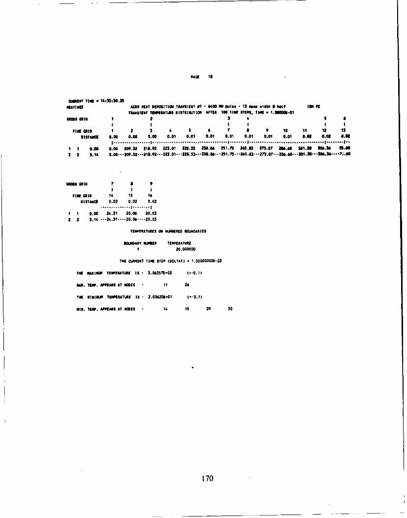
PAGE Is

081o11 TIva a 14:33:30.25

IATINGS ACR NEAT DEPOSITIO TRANSIENT l 6400 M plse - 13 mac width a haf IBM PC

TRANSIEMT TEMPERATURE DISTRIBUTI AFTER 10 TIME STIP, TIME - 1.0000U.O1

aSm ID 1 2 3 4 5 6I ! I 1 1 1

FINE RID 1 2 3 4 S 6 7 a 9 10 11 12 1i

DISTAUNC 0.00 0.00 0.00 0.01 0.01 0.01 0.01 0.01 0.01 0.01 0.02 0.02 0.01

I .................................................... I . I...................... I ........ a..

1 1 0.00 0.00 209.3z 21.92 2.01 23.33 23.1 21.75 265. 23.07 .40 3I.3 31.3 8.0

2 2 3.14 0.0- ... -10.92. 3.01-" 2n.33--3..2--' 5 ... US .- .0. -- 1.U- . .. ....

am 0GRID 8 9

! I I

FIN GRID 14 1s 16

DISTANCE 0.02 0.02 0.02o.............. I ........ I

1 1 0.00 24.31 20.06 20.03

a 2 3.14 ...- 24.31 .... 20.06 .... 20.03

TEMPIRATURES OlN MUIEREED IPiOARIES

S1UDARY WUUllE TEMPERATURE1 20.000000

INE CLAI11T TIME STEP (DELTAT) - 1.000000000-03

TE IMAII.I TEMPERATURE IS 3.06357D.02 (*-0.1)

MAX. TEMP. APPEARS AT DS H 11 26

TI MINIM. TEMPERATURE as 2.006200.01 (C-0.1)

MiN. TEMP. APPEARS AT NiDOS 14 Is 29 30

170

PAGE 19

CURRENT TINE 14:36:26.N

HKATIM0S Actl NEAT DIPOSITION TRUASIENT a1 - 6600 ON put" 13 Nw vidth a half [on PC

TRANUISIENT TIMPERATUiE DISTRIBUTION AFTER 500 TIM STEPS, TIME a 5.000000-01

a S GIO D 2 3 4 S 6I i I I I

FIN EID 1 2 3 s $ 6 7 a 9 IS 11 1& 13

OISTANCI 0.00 0.00 0.00 0.01 0.01 0.01 0.01 0.01 0.01 0.01 0.02 0.02 6.02I ................. I ............................. I . I..................... a ........ I-

1 1 0.00 0.00 222.91 223.12 225.70 WA31.5 239.16 2A..06 278.61 281.2S 2N6.11 219.16 231.51 45.602 1 $.14 0.00---. 22.91-- ?...2. 12- ...225. ?0-- .. 21.35 -.-. 239.18- .. -2".06- ... 78.61- ... M.25- -- -286.11o--.210. 16---. 206.51 .... 45.00

GROSS GID 7 aI I I

FMI GRI*D 14 IS 16

DISTANCE 0.02 0.02 0.02

o- * * . . . . .- - * - * . . . . . . . .I

1 1 0.00 43.79 21.70 21.50

2 a 3.14 -.-- 3.?9 ... 21.70 .... 21.50

TENPERATUlRES ON MUP48ERE0 IOUNI)ARIES

SINUARI• UMBER TEPERATURE1 20.000000

THE CURRENT TINE STEP (VEVTAT) - 1.000000000-03

THE MAXIMU TIEMPERATURE IS- 2.891166-02 C-0.1)

PAX. TFIM. APPEARS AT MODES - 10 25

THE MINIMA TEIPERATURE IS - 2.150100.01 (#-0.1)

MIN. TEOP. APPEARS AT HOVES Is 30

TAELE FOR SPECIAL MIOITOING OF TEMPERATURES

NUER OF TIME 82s-moe es-8 .... . .UWE ri0 s AND TEMPERATURES

TINE STEPS

1000 1.00000.00 1 2.260030-02

171

PAGE 20

08I3T TIME a 14:37:25.26UAIJOS AMR WAT DEPOSITION TRANSIENT 61 - 4OO 0 Put"s - 1 WSW udth 8 hatf SIN PC

TRANSIENT TEMERATURE DISTINUTION AFTER 1000 TINE STEPS. TIM * 1.0000000Gem GRID 1 2 46

I I I I I

FIRE GRI I a 3 4 $ 6 7 8 9 10 Ii 12 13DISTANME 0.00 0.00 0.00 0.01 0.01 0.01 0.01 0.01 0.01 0.01 0.02 0.02 0.02

I ................. I ................................... I ........ I ................................... I ........ I--

I 1 0.00 0.00 226.80 226.96 228.94 233.37 238.15 240.93- 261.96 22. M282.0 1111.36 277.28--6 .04

om0 GRID 7 a 9i I I

FINE GRI0 14 Is 16OISTANCE 0.02 0.02 0.02

.. o.......... Ioo ........ I

I 1 0.00 62.87 25.95 25.59

2 2 1.14 ... 62.6? .... aS.9s .... 25.59

TEMPERATURES ON NUMBEED11 SOJNOARIES

BOUND4ARY 3UM111 TENPEIATUIE

1 20.000000

tE CURRENT TINE STEP (OELTAT) a 1.000000000-03

131E NAIIW TEMPERATURE 15 - 2.828540-02 (*-0.1)

NAX. TEMP. APPEARS AT 301S - 9 24

TNO NINIMU TEMPERATURE IS - 2.559260.01 (-0.1)

Nil. TEOP. APPEARS AT NODES - 15 30

172

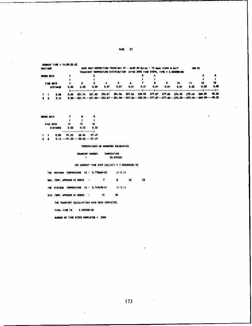
PAWE 21

lhURNT TIME 1 4:39:22.12NEATINGS ACIN NEAT SEPOSITION TRANSIENT 51 - 400 ON paat" - 13 Mac uidth 8 half Is" PC

TRANSIENT tEMPERATULE OISTRIIIUTION AFTER 2000 TIN STIPEPS TIME a 2.000000.00

NA001 eta 3 4 5 6I I I II

ulag lG0 1 2 3 S 6 7 a 9 10 tl 12 is

DISTANCE 0.00 0.00 0.00 0.01 0.01 0.01 0.01 0.01 0.01 0.01 0.02 0.02 0.0I ................. I ............................. I . I..................... I ........ I--

1 1 0.00 0.00 231.74 231.82 -.61 2.9 23727.2 236.931 27.8? 2•. M 276. . 273.6 1169.29 W.323 .t4 0.00* ...2314...- -231.Un-- .. •. ZU "" .. Z3-% ..9" "2?.2" ... 238.911-277.117i...2??. ..M .33 - ..]2'T.64 "'9.2'.2

410l5010 7 a 9I I I

FINE MID 14 1 16DISTAMNC 0.02 0.02 0.02

* ......... I ..... I

1 1 0.00 91.20 31.06 37.492 3 3.16 ... 91.0 .... 38.06 .... 37.,-9

TEMPERATURES ON 14UMI6E0 OUAINARIES

BOUNDiARY INIER TEMPERATURE

1 20.000000

INS CURRENT TINE STEP (OELTAT) 1.000000000-03

TiE UAXIUM TEMPERATURE IS 2.T77'002 (-0.1)

oxi. TEIP. APPEARS AT NlESIS 7 a 22 23

IN[ NINIUM TEMPERATURE IS 3.7,9490-01 (4-0.1)

KIi. TIP. APPEANS AT NI$C0EE Is 30

TNE TRANSIENT CALCULATIONS NAVI SIEEN COPLETED.

FINAL TINE IS 2.000000.00

EUNlt Of TINE STEPS COMPLETEO & 2000

173

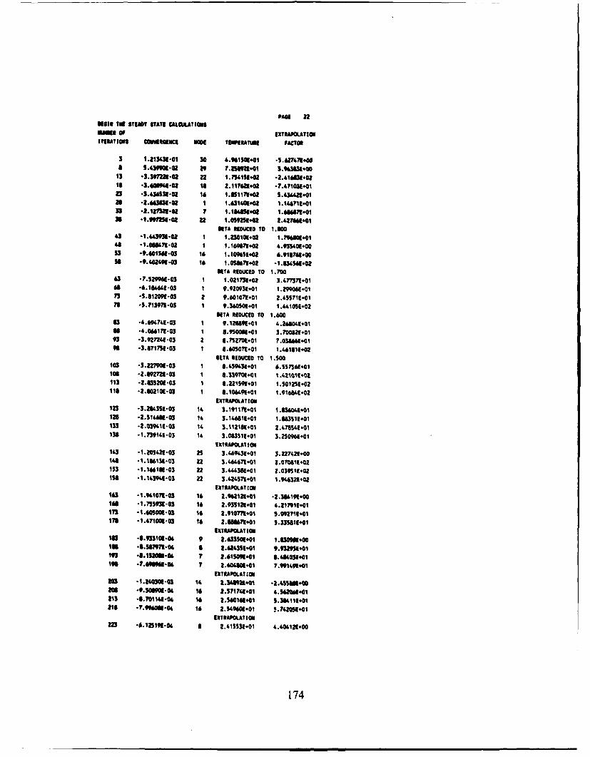
PAGE u20141u mg ITIAO 611TATE CALSIALAT 2036V1610 OF EXRTAPOLATION21619RAION CIwwww" NONUS TIMPEATWIM FACTOR

3 1.2131.31-01 30 41961540.01 *5.6171.71-0a 5.1.3990-0 29 7.23092.0¶ 3943638.0

13 -3.39122102 2.2 1.73415142z -2.1.16031#02Is -3.0000144-02 1s 2.117029.02 *7.1.710M1.0123 *31.3431-02 16 1.111171#02 5.451.21.01BE -2.466531-02 1 1.6311.01.02! 1.146M.0133 -a.127321.0 7 1.1660151#02 1.600790013B -1.19172"42 22 1.0592514 2.4271641.01

811A 29EJDCE TO 1.800043 .-1443930102 1 1.230109.02 1.790101440 -1.004171-02 1 1.169671.02 1.935401.0033 4.9.01561-03 16 1.100151.02 6.914761.00so .9.4024.91-03 16 t.050671.02 -1.631.541.02

MITA REDouctS TO 1.70043 -7.52994-03 1 1.021731.02 3.4.77371.048 -6.1&161.1-03 1 9.920931.01 1.299001.01

73 -5.81209103 2 9.601071.01 2.1.55111.0176 -5.713972-OS I 9.360501.01 1.1.1ost.02

BETA REDLUCE TO 1.60063 -4.691.741-03 1 9.12401M.01 4.268041.01of .-4046171-OS 1 $.950001.01 3.700521.0193 -3.92721.1-03 2 0.752701.01 7.036661.01

90 -3.071731-03 1 11.6050711.01 1.4.61411.02BETA REOUCIG TO 1.500

103 -3.22790-03 1 8.4.591.31.01 6.557541.011061 -2.092721-03 1 41.33970.01 I .42111af03113 -2.635201-03 1 6.221591.01 1.501251.02110 -2.002101-03 1 0.104491.01 1.91644102

EXTRAPOLATION2133 -3.201.35-03 11. 3.191171.01 1.636041.01120 -2.5146811-03 14. 3.11468111.01 1.6113519.01133 -2.0391.11-03 11. 3.112161.01 2.4YSSI.1.0136 -1.73911.1-03 11. 3.06351101 3.250961.01

EXTRAPOLAT ION11.3 -1.M205.2-03 25 3.1469431.01 3.227421.00140 -1.186139-03 22 3.4.61471+01 2.070111.02153 -1.6101S-03 22 3.144301.0 2.039S11.021se -1.14.3M4-03 22 3.1.21.51.01 1.944321002

EXTRAPOLAT ION13 -1.9414711-03 14 296212141i -2.6441900

140 -1.755931-03 16 2.935129.01 4.2179W101in -1.605001-03 16 2.91o77o4l 5.092711.0117$ -1.1.71009-03 16 2.66006714*1 5.335011.01

EXTRAPOLATION163 -0.933101-04 9 2.433509+01 1-930901600In -0.56797-06 8 2.621.351.01 9.932931.019 -0.15206-06 7 2.015001001 8.1.04031#01

196 .7.9091-0. 7 2.6048011.01 7.991491.01EXTRAPOLATION

30 -1.21030-03 11 l.31.621.0 -1.4%sUI.002no -9.5 .090-0 16 2.571741.41 6.54204*14213 -0.10111.1-06 16 2.540141401 5.361.111.01R10 7-1.90601-04 16 2.54101.01 5.71.205101

EXTRAPOLATION.223 -6.125191-04 6 2.1.1531.001 4.1.01121.00

174

2na *5.84"11-04 a 2.4oa341-01 9.05399101

175

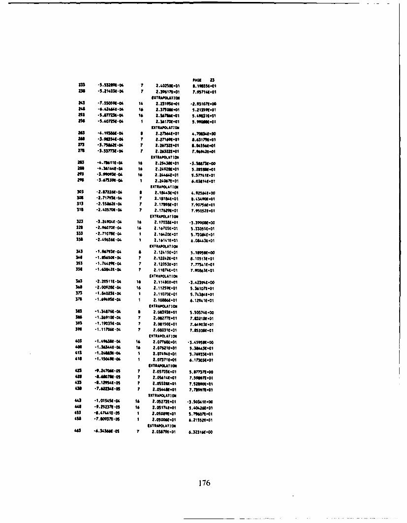
PACE 23233 -5.s3289-o 7 2.402581001 3.lW55l.0l2no -5.214039-04 7 2.396171.Ot ?."57141#01

EXTRAPOLATION263 *7.5S0591-06 16 2.231951.l -2.9310711000268 -6.4241141-06 16 2.375GK010 5.213S99-1.as3 *5.4r=-04 14 2.367164401 5.496311.*0i

258 5o72sa-*4 1 2.361 oi*o1 S.9901.0

EXTRAPOLAT ION263 -4.1931161-06 8 2.275641001 4.704W-100so8 *3.98356-06 7 2.271699*01 8.631791.271 *3.75062E-04 7 2.267321*01 8.045581.01273 *L.53773-o' 7 2.26322101 7.%%969201

EXTRAPOLAT ION26 -6.7`86111-04 18 2.256381.01 -3.388731.028 *4.361661-04 16 2.269231.01 5.2858810129 -3.9903106 16 2.244869401 5.71.1296 -3.675399-06 I 2.240671.01 6.038141.01

EXTRAPOLATION303 -2.972261-06 a 2.184431.01 4.925661-0030B *2.717M3-04 7 2.160614101 6.434901.01313 *2.55862-06 7 2.173981401 7.90796101313 *2.605701-06 7 2.176291.0 7.950521.01

EXTRAPOLATION323 -3.24904E-04 16 2.i70381.0 -3.399081.00328 -2.96070 -04 16 2.16005i.0¶ 5330551.01"33 -2.7107U1-" 1 2.964201.01 5.720690101336 -2.696SW-04 1 2.16w16¶u0 6.084439-01

EXTRAPOLAT ION363 -1. 96931- 04 a 2.124151.01 5.189581.00368 -1.I63801-04 7 2.12242E-01 8.105131.0l353 -1.764299-04 7 2.120531.01 7.77341101358 -1.8396201-6 7 2.116741.01 7.90163.01

EXTRAPOLAT ION363 -2.20511-06 18 2.116801.01 -3.423941.00368 -2.009261-06 16 2.l12S9E.Ol 5.361071.01373 -1.860231-04 I 2.110701.01 S.743849.01378 -1.694959-04 1 2.108W6101 6.129411.01

EXTRAPOLAT ION383 -1.U687611-04 a 2.063931.01 1.505761.003111 -1.269101-06 7 2.082771.0 7.832181.01393 -1.190351.04 ? 2.0815S01.01 7.60E0390 -1.11706-06 7 2.080311.01 7.853081.01

EXTRAPOLATION603 -1.6963M1-064 16 2.077611.01 -3.459581.00416 -1.363461-06 16 2.076211.01 5.386631.01413 -1.1488M104 1 2.076941.*01 5.76"933101418 -1.150491-06 1 2.073711*01 6.173031.01

EXTRAPOLAT ION423 -9.267061-0 ? 2.0s57051.0 5.8771.00428 -6.6781.05 ? 2.05S6141.01 739109711.01433 -8.12941-0s 7 2.055231.01 7.52390.0438 -7.62236-05 7 2.054681.0 7.739971.01

EX71AMOATIoN"43 -1.01S451-04 16 2.052721.01 -3.503611.00668 -9.252371-05 16 2.051761.01 5.604269401653 -8.0441l1-05 1 2.05089101 5.70607to1458 -7.809371-0 1 2.050061.01 6.215521.01

EXTRAPOLAT ION663 -6.343691-5 7s 2.038791.01 8.323161.00

176

f.~-s.~oai~o 7 2.038172-01 ?.3591S9.Ol

177

PAGE 26

673 5.55701.5 7 2.037OWg01 7.615231.0

EXTRAPOLAT ION63 -6.091691-05 16 2.035871.01 -3.593741.0061 .. 279321.0 16 2.0311211.01 1.6.22471.01'93 .M5201*0 16 2.036601.01 S.773221.0

696 -9.301799-05 1 2.0160111#01 6.257191.01EXTRAPOL.ATION

503 *6.I3521.05 7 2.026621001 6.63795.00$01 *6.067581-05 ? 2.026001-01 7.2156711.01Si13 *3.7W901.@ 7 2.025601.01 7.30706".01513s *3.556m51.s 7 2.025231.0 7.654W6101

EXTRAPOLAT ION.1 *.67631-os 16 2.0266W101 -3.609561.0052 *.2m339105 16 2.024019.01 5.660011.01

533 -3.906236-05 16 2.02360101 5.307711.01533 *3.GM055-05 16 2.02322E.01 6.266871.01

EXTRAPOLAT ION563 *2.91?59E-05 7 2.013031.01 7.43947t.005S" *2.7S621-05 7 2.01774E-01 7.054401.01553 -2.5"9S96-05 7 2.017671.01 7.306731.01558 -2.430951.05 ? 2.017z22go1 7.Se6051.o¶

EXTRAPOL.ATION563 *3. 176641.-05 16 2.01670[.0¶ *3.67026100563 -2.895319-05 16 2.016401.01 S.451651.0137 -2.653s71-05 16 2.01612E.01 5.636511.01573 -2.44690E-05 16 2.01587E.01 6.303941.01

EXTRAPOL.ATI ON563 -2.0666W-05 7 2.01232E.01 7.305731.00sea *1.903761.03 7 2.01213u01 6.96177t.01593 -1.776371-OS 7 2.0119&E.01 7.166651.01593 -1.6S395-05 7 2.011771.01 7.554261.01

EXTRAPOL.ATION603 -2.1517191-05 16 2.011431.01 .3.717651.00606 -. 96649E-05 18 2.01122E.01 5.67553t.01613 -1.3802891-05 16 2.011061.01 S.866981.01616 -1.663151-05 16 2.010861.01 6.342191.01

EXTRAPOLATION623 -1.403121-05 7 2.00b61.0, 8.5193651.00623 -1.3043411-05 7 2.0O0130101 6.a1307t.01433 1.21¶4jg.05 7 2.008161.01 7.057721.01

638 -1.3661-O 7 2.00806101 7.69097',:.01EXTRAPOL.ATION

643 -1.465331-05 16 2.00766101 -3.756631.00668 -i.3UW06-oS 16 2.0077M01.0 5.403961.01653 -1.22321-OS 16 2.007571.01 5.693671.01654 -1.`130611-O3 16 2.007451.01 6.36004.01

EXTRAPOLATION"43 -9.631501-06 7 2.0057-01. 9.41"71000

178

PAGE 25

COAENT TINE * 14:40:16.40KNAYGS ACRA NEAT DEPOSITION TRANSIENT 9l1 • 600 W put" - 13 mme m.idth a altf Ip PC

STEADY STATE TEMPERATURE DISTRIBUTION AFTER 603 ITERATIONS, TIME a 2.00000S.00

am GRID 1 2 3 4 6 6I I I I !

FINEUIO C 2 3 4 3 6 7 S 9 10 i 12 '13DISTANCE 0.00 0.00 0.00 0.01 0.01 0.01 0.01 0.01 0.01 0.01 0.02 0.02 0.02

I ................ I ................................... I ........ I ................................. I ..

1 0.00 0.00 20.04 20.00 20.00 20.06 20.00 20.00 20.06 20.00 20.00 20.06 20.06 2O.0O2 a 3.14 0.00 .... 20.03 .... 20.06 .... 20.06 .... 20.04 .... 20.04 .... 20.04 .... 20.06 .... 20.06 .... 20.06 .... 2O.06 ---- 20.06 ... 20.06

GROSS Clo0 7 8 9I 1 I

fIlN GRID 14 is 16BISTANCE 0.02 0.0* 0.02

• .... o.. ..... I ........ I

1 0.00 20.04 20.04 20.042 2 3.14 ... 20.04---.20.04 .... 20.04

TEMPERATURES ON NUMBERED BUJNOARIES

'DUJI ANY NUMBER TEMPERATURE1 20.000000

174 MAXIMU TEMPERATUIE IS 2.005910-01 (--0.1)

MAX. TEMP. APPEARS AT NMOES 1 2 3 4 5

6 ? a 9 1011 12 13 14 1516 17 18 19 2021 22 23 24 25

26 27 28 29 30

TlE MINIIM TEMPERATURE IS 2.005910-01 (--0.1)

NIN. TEMP. ADPPEARS AT NODS 1 2 3 4 5

6 7 a 9 1011 12 13 146 Is16 17 is 19 2021 22 23 24 252• 27 28 29 30

TiS WTEM? STATE CALCULATIONS AVE IEN COMPLETED.

mIgif OF ITERATIONS COPLETED a 663

....... WEXXXXX XXX XXXXXXXZ2O12CxOn X2• U IrXX

V AN SUPPOSE D0 PUT A BLANK CARD BETWEEN JOBS.

I M UVI lOT FOUID IT. I IBALL O OAMED AND WITE TNEC I PAVI JUST Km AS ?us JOB DESCRIPTION FOR TNE NEXT JOE.

179

Appendix C

Matlab Sample Data File - no noise case 181

Matlab Sample Input File - no noise case 182

Matlab Sample Output Plots - no noise case 184

Matlab Sample Data File - two percent noise case 191

Matlab Sample Input File - two percent noise case 193

Matlab Sample Output Plots - two percent noise case 195

Matlab Sample Output Plot Generation File 202

180

aO-9.82 18e4;al=-4.0822e-7;a2=1. 1773e-10;W 1. 113e-I1;bl-1.5402e4;b2=-4.0805e4g;cO=78.381;cI=0.3393;c2-4.9181e-5;d=4 189.S;dl=-0.61063,d2-0.008881 1;gO=1002.91gl=.O. 1599;g2=-0.0028345;m2=-0.0151;ml=2.930S;mO=-49.79;

A14.0;df-3550;Vf=0.09866089.dt=0.05;t=6.3c-7.Vm=0.045434752-,cpm~=4182;Tm7=20.0;,Tnma( I)20.0;Tpool=20.0:Tfint--25;Pint=3e:Tfr-Tfint;Tfm=Tfint:TfTl(l.1)=Thn:P-Pint.reactfbint=0.0;for i=1:3000Tfrl( 1,i+ I )=Tfr-A*dt*(bO*Tfr+b1 *TfrA2+b2*Ttr-3)/(dl*Vf)..

+A~dtTm*(bO+bI *Tft.b2*TfTA2)/(df*Vf)..+( 1.t)*dtP*(aO+al*Tfr+a2*Tfr A2)I(df*Vf).

beaindt((A*(cO+cl *Tf,+c2*TfrA2)*(Tfr-Tm))+(t*P))/...((gO+gl Tzn+g*TMA 2)*(dO+d I *Tm+d2 *TMA 2)*Vm):heatour-dL(mO+mI Tm4 2*TmA,2)*2(Tm.TpooI)/((gO+gI Tm+g2*TMA2)Vm)-.Tzna(i+ 1)=beatin-heatout+Tm:Tm=Tma(i+ I);Tfr=Tfirl(l,i+1);if i<100P-P+3.997e4;elseP-46;endendfor i 1: 3000

reacttb( .iH=Tfrl(l1 i)-Tfint)*(-3 .85-(730/(273.1 5+Tfrl( I.i)))) le-SI0.0073:

181

80=0.;at=4.0822;,a2=1. 1773c-1O;;

bl0.:

bZ-4.OSO5c-8;c0-78.38 1;c1-0.3393;c2=-8.91g1e-5;do=4189.8:.dl1-O.61063.d2-0.008881 1;g0=1002.9;g1=-0. 1599,g2=-0.0028345;ni0-49.79;ml=2.9305:.m2=-0.0151.A-14.0;df-i35SO;Vf-0.09866089;d1--0.05:t=6.3e-7;dm--998.20323:Vm=O.045434752:cpm=4182;Tm=20.0:.TrnI(l)=Tm:Tpool=20.O:Tfint=25.Pint-3e3;reacfbmn( I)0.O:TfmnTfint:P-Pint:P1(1 )Pint;datam=ITfm bO bl aOl:F11l -A~dt*(b0* 1e-1+2*bl e-4*Thm+3 *b2*Tfin/A2)/(df*Vf).+A~dtTm*(bl * le.4+2*b2*Tfmn)/(df*Vf)+dt*(l -t)*P(al * e-7+2*a2-)Tfin)/(df*Vf):F2=A~dtle I- *(Tm-Tfm)/(df*Vf):F3=A~d11e-4*(Tm*Tfm.-TfmA 2)/(df*W1):F4=( -t)*Pdt* Ie~4/(df*Vf);F-[FIF2 F3 F4,0 10 0;00 10;0 00 1]-.Eininv(F*F);

sw&iO.O;bOsum-O.0;bOave( 1)0.O;

bisumin.0;

20ave(1)0O.0;for i- 1: 3000X=[Tfm bO bI aOl';-h-(-3.S5+730*Tfin/(273.1I5+Tfm)A2..730/(273 I S+Tfm)-730*TfinhI(273. 15+Tfm)A2...

182

)* le-SI.0073;H'1b 0 001';

L-E*Hinv (0):YrcatOXI 1,i);xhat-X+L*(Y-(Tfm-Tfint)*(-3.85-(73O/(273. IS4Tfn)))* Ic-5/.0073)-datam-ldtam;xhat'J:Tfin---at(1. I)-,reactlbm(i+l)=(Tfm-Tfint)*(-3.85-(730/(273. 15+Tfmn))) Ie-SI.0073;Tml(i+l)=Tm;bO=xhat(2, 1);blu-xha(3,1);raO-xhamt(4, 1);bOsum-Wb*i+bOsum;blsum-bl~i+blsum;aOsum-aO*i+a~sum:,sumi~i+sumi:bOave(i+1)-bWsuxn/sumu:blave(i+1 )wblsum/sumi;aOave(i+l)ina~sum/sumi.,j=j+ 1;Tfin I=Tfm-A~dt*(bO* Ie- I *Tfm+b I I 1e-4*TfmnA 2+b2*Tfkn A3)/(df* Vf)...

-'A*dt*Tm*(bO* Ie- I +b I* Ie4*TTfin~2*fnA 2)/(df*Vf)...+(I -t)Odt*P I(i)*(aO* I1e4+a I * I c7*Tfm+a2*TfmnA 2)/(df*Vf);.

Tmcal-Tm+dt*(A*(cO+c I Tfiu+c2 *TfhnA2) (Tfin-Tm)+P I(i)* t-...(mO+mI*Tm+m2*TmA12)*(dO+dI *Tm+d'-*TmA2)*2*(Tm-Tpool))/..((gO+gl *TM+g2*TMA2)*(dO+dl*Tm+d'2*TMA 2)*Vm);F I I A*dt*(bO* I e- 1+2 b I * IleA*Tfmn+3 *b2 *ThtnA2)/(df*WO...+A*dt*Tm*(bl * le.4+2*b2 *Tfin)/(df*VI)4.dt*(1.-t)*P1 (i)*(al 1e1 c7+2*a72*Tfm)/(df*Vf):F2=A~dI* c-l (Tm-Tfin)/(df*VfO.F3=AMdtl*e4*(TM*TfiniTfmnA2)/(df*Vf):.F4=( 14)*Pl(j)*dts1e.4/(df*Vf);F=IFI F2 F3 F4:0 10 00;00 10:0 0 01]:ffj=3001

El F*Ea*F;end

Tm=mcl;

Tin-Tfml;if i<100P-P+3.997o4;PI(i+i)=R,elseP=4e6;P1(141)-P-,

end

183

Feedback Reactivity - Model and Actual

-0.5

-1.5

-2Al -2.5-

.1 -3-

-3.5

-4

-4.5

0 20 40 60 80 100 120 140 160

Time (seconds)

184

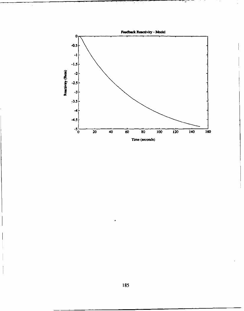
Feedbac Reactivity - Model

0

-0.5

-1

-1.5

-2--2.5

-3-

-3.5

-4

-4.5

0 20 40 60 80 100 120 140 160

Tune (seconds)

185

Estimated Model Pimmeters

10

6

2 4

2-

0

"20 20 40 60 80 100 120 140 160

Time (seconds)

186

Average Model Parameters

10

6

4-

2-

0A

-210 20 40 60 80 100 120 140 160

Time (seconds)

187

x106 Reactor Power

4

3.5-

3

2.5

2-1.5

1

0.5

010 20 40 60 80 100 120 140 160

Time (seconds)

188

Fuel Temperature - Model and Actual

900

800

400

0 20 40 60 8s 100 120 140 160

Time (seconds)

189

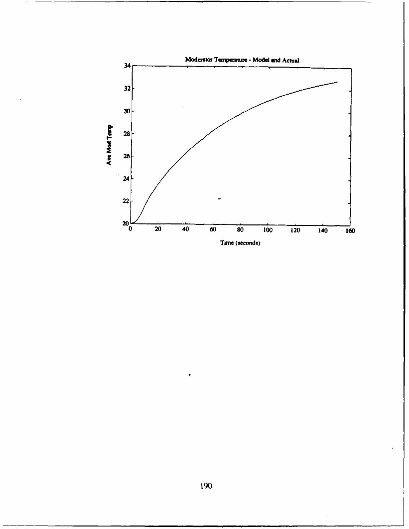
Moderator Temperature - Model and Actual34

32

30-

~28-

26-

24-

22-

200 20 40 60 80 100 120 140 160

Time (seconds)

190

&0-9.8218e-4;a&m-4.0822e-7;a2-1. 1773e-1O;,bD1.1 13e-1;bl-1 .5402c4;b2-4.OSO5e-8;cOin78.381:c1=0.3393;,c2=48.918le-5;dO-4 189.8:.dP=-O.61063;d2-0.008881 1;g0-1002.9;gl=-O. 1599;92=-0.0028345;M2=-0.0151;ml=2.9305;MO=-49.79-:A=14.0;df-3 550;-Vf-0.09866089:dt=0.05:t-6.3e-7.dm=-998.20323-.Vm=0.045434752;cpm=4 182;Tm=20.O;Tnia(lI)=20.0.Tpool=20.0;.Tfint--25;Pint=3e3-.Tfr-Tfint.Tftn=Tfint,;

P--Pint;reactlbint=O.0:for i=1:3000Tfrl( 1.i+ 1)=Tfr-A*dt*(bO*Tfr+bl *TfrA2+b2*TfrA3 )/(df-Vf)..

+A*dt*Tm*(bO+bI *Tfr+b2 *TfrA 2)/(df* Vf)...+(I -t)*cft*P*(aO+a I *Tfrs~a2*TfrA2)/(df'*Vf);

hetin~d*((A*(cEJ+c1*Tfr.+c2*TfrA2)*(Tfr-Tm))+(t*P))/..((gD+gl *Tm+g2*TMA2)*(dO+dl*Tm~sd2*TMA 2)*Vm),heaouxt-di(mD+ml *Tm+m2*TMA 2)*2*(Tm-Tpool)g((gD+gl *Tm+g2*TMA 2)*Vm):Tma(i+1)=heatin-heatout+Tm;Tm=Tma(i+ 1);Tfi-Tfirl(l.i+I);if i<100P-P+3.997e4;elseP-4e6;endendfor i=I.+3000

reactfb( I.i)=(Tfril( .i)-Thint)*(-3.85-(730/(273 I 5+TfrI(l1,i))))* le-5/0.0073.

191

endfor i=1: 3000

reactfb( ,i)-reactlb( 1.i)4O.02 *reactfb( 1 j)*( I -2*rand).end

192

aO=O;al=-4.0822:.a2=1. 1773e-1O::

b2=-4.0805e-8;cO=78.381;cl=O.3393-,c2=-8.918le-5;do-4189.8;d1=-O.61063;d2=0.008881 1;gO=-1002.9:.g1.-O. 1599;g2=-0.0028345;mO=-49. 79;,ml=2.9305:m2=-0.0151.A=14.0.df--3SO;VfO0.09866089;dt=0.05:t-6.3e-7.dm=998.20323:VmO0.045434752;,cpm-4182,Tm-=20.O:.Tml(1)=Tm;Tpool=20.O;Ttint=25:Pint-=3e3:reacffbm(lI)-O.O,Tfim=Tfint;P-Pint.P1(1)=Pint-,datani=[TfhinbO bl aOl;F11l -A*dt*(bO* le- I+2*bI l e4*Tfm+3*b2*TfmnA2)/(df* Vf)...+A*dt*Tm*Qbl * Ie-4+2*b2*Thtn)/(dfIIVf)+dt*( l-t)*P*(a I *le-7+2*a2*Tfm)/(df* Vf).F2=Adt* le- *(Tm-Tfm)/(df* Vf)F3=A*dt* le~4*(Tm*Tfm-Tfn A 2)/(df*Vf);F4=(1-t)*P*dt* lc-4/(df*Vf);Fj[FlF2 F3 F4;O 10 0;0 0 10,00 0 11:E=inv(F*F);j-0.0;sumi=0.0;bOsum=0.O;W~ave( 1)0.0;blsum=0.0:blave( 1)0.0;aOsum=0.O;20aVC( l)0.O;for i-1i:3000X=fTfmn 1, bi aOJ':h=(-3.85+730*Tfn/(273 . 5+Tfrn)-2-7301(273. I 5+Tfm)-730*Tfintl(273. I 5+Tfm)A,2..

193

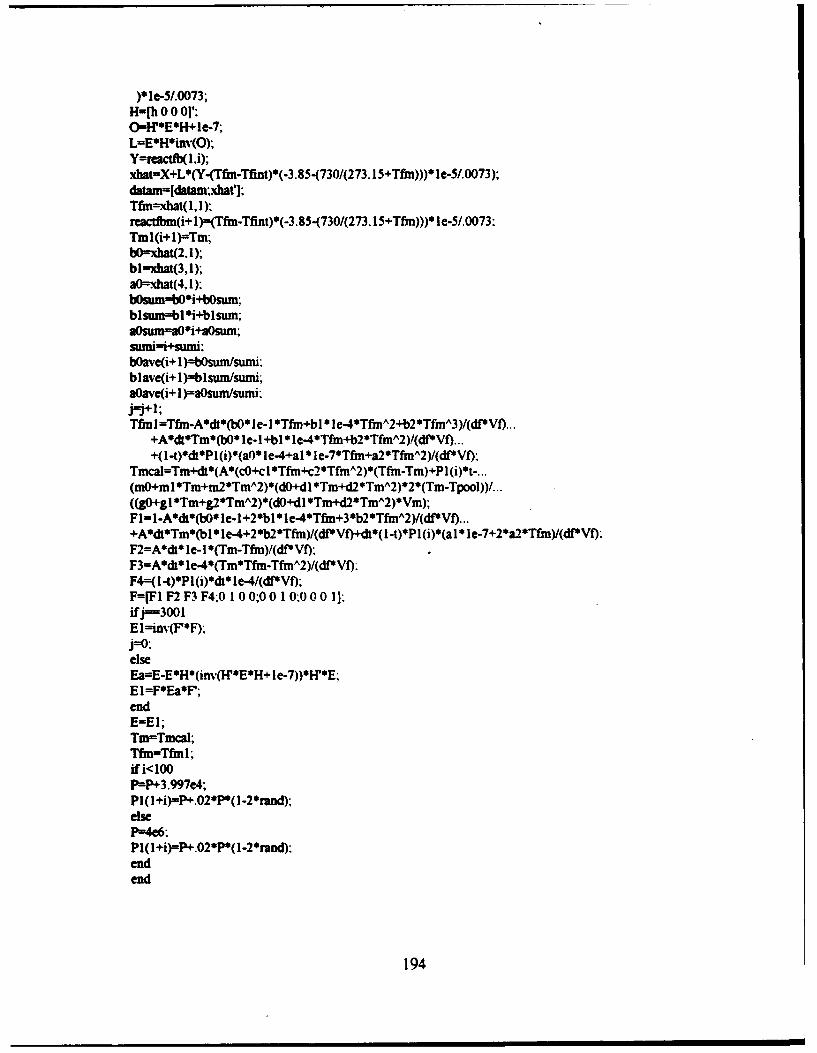
)*le-RI0073;H-[h OOj'-.O=HTE*H+le-7;L=E*H*inrv(O);Y=reacdb(l.i);xbat-X+L*(Y-(Tfm.-Tfint)*(-3 .85-(7301(273. 15+Tfln)))* le-5I.0073);datamljdatam~xhatl;Tfin--hat(l, 1)-,reacdbm(i+l)=(Tfin-Tfint)*(-3.85-(73O/(273. 1 +Tfmn))) Ie-5/.0073:.Tml(i+l)'Tm;WDxbat(2, 1);bl-xbat(3, 1);aO=.xhat(4. 1):bWsum~bO~i+bOsum;blsum-bl~i+blsum;aOsum=aO*i+aOswn;sumiii+sumi-.bOave(i+ 1)=bOsumt/sumi:.blave(i+l)=blsum/sumi;soave(i+1)=aosuni/sumi:j=j+ 1;Tfin 1Thn.A*dt*(bO* I e-1I *Tfmn+b I *e-4*TfmA"2b2 *TfMA 3)/(df*VO).

+A*dt*Tm*(bO* le-l +blI * 1e~4*Tfkn+b2*TfMA 2)!(df* Vf)...+(I -t)*dt*Pl (i)*(aO* le-4+alI * I e.7*Tfin+a27*TftuA2)/(df*Vf).

Tmcal=Tm+d1*(A(cO+c I *Tfifl+c2*TfMA 2)*(Tfin-Tm)+Pl(i)*t-..(mO+ml *Tm+m2*TMA 2)*(dO+d1 *Tm+cI2*TMA 2)* 27*(Tm..TpooI))/...((gO+gI *Tm+&2*TMA2)*(dO+d1 *Tm+d2*TMA2)*Vm);Fl= I-A~dt*(bO* le- I+2*bl * 1e4*Tfmn+3*b2 *TfmnA2)/(df*Vf)...+A*dt*Tm*(bl 0 le-4+2*b2Tfmn)/(df*Vf)+dt*(1 -t)*P1(i)*(al I le-7+2*a2-)Tfn)/(df*Vf).F2=A~d* Ile-1I *(Tm-Thin)/(df*Vf):.F3=A~dt* le4*(Tm*TfmnTfin A2)/(df*Vf).

F=[F1F2 F3F4;0 10 0;0O0 10.0 00 11.ifj==3001E 1-irn(F*F);j0O.elseEa-E-E*H(inv&RE*H+ Ile-7))*If*E,E 1=FEa*F;endE=EI;Tm=Tmcal;Tfm=-Tfmnl;if i<100P-P+3.997e4;Pl(I+i)=P+.02*P( l-2rand);elseP-4e6.Pl( l~i)=P+.O2*PO(1-2*rand):endend

194

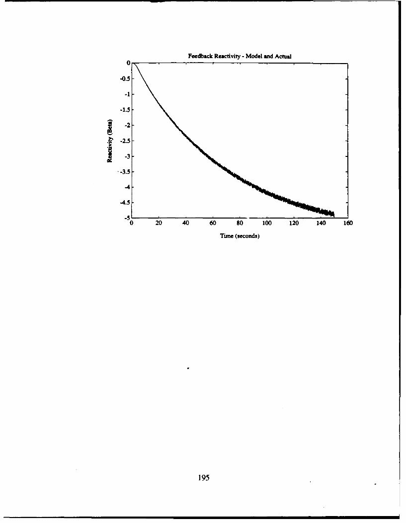
Feedback Reactivity - Model and Actual

0

-0.5

-1

-1.5

S-2

. -2.5] -,

* -3.5

-4

-4.5

0 20 40 60 80 100 120 140 160

Time (seconds)

195

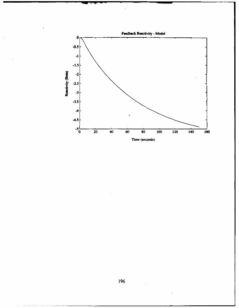
0 Feedback Reactivity - Model

-0.5

2-I-1.5

-2.5

-3-

-3.5

-4

-4.5

"0 20 40 60 80 100 120 140 160

Time (seconds)

196

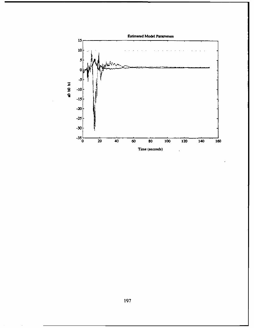
Estimated Model Parameters

5

10 -10-0

-5S -10 -

-15

-25

-30

-35"0 20 40 60 80 100 120 140 160

Time (seconds)

197

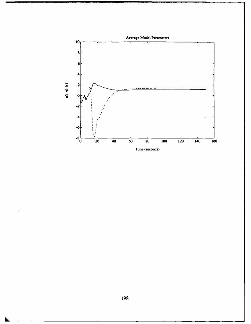
Average Model Parmeters

10

S

6

4

2-

0 20 40 60 80 100 120 140 160

Time (seconds)

198

Fuel Temperature - Model and Actual900

800

700

~400-

200O

100

0 2•0 40 60 80 100 120 140 160

Time (seconds)

199

x106 Reactor Power

4.5

4-1

3.5

3S2.5-

2-

1

0.5

0 20 40 60 80 100 120 140 160

Time (seconds)

200

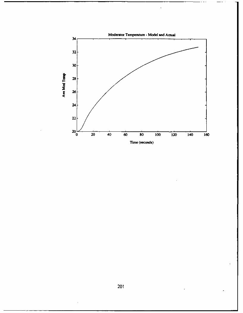
Moderator Temperature - Model and Actual

34

32

30-

28-

0 26-

24-

22-

2010 20 40 60 80 100 120 140 160

Time (seconds)

201

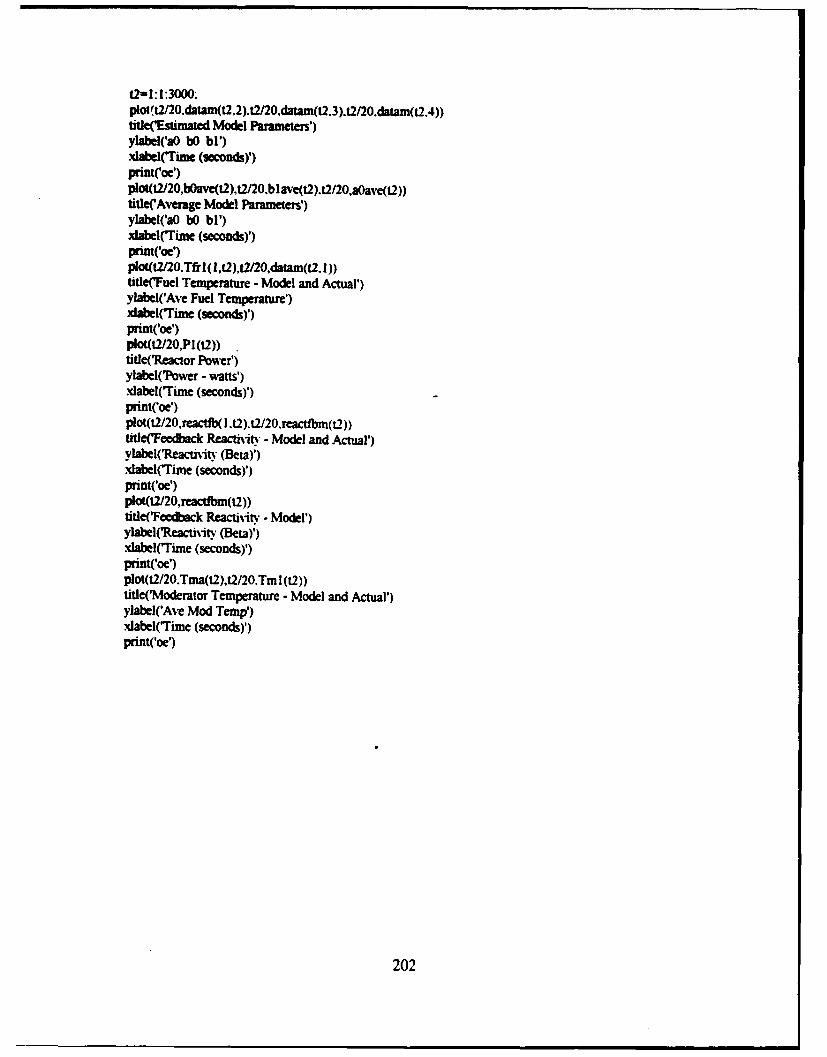
t2-1:1:3000-.

title('Estimated Model Parameters')ylabel('aO bO bi')Xlabe~'run (Seconds)')print('oe')Plot(t2/2.O.ve(t2),t2/2O.blave(t2)it2/2o,aoav'e(t2))titlerAverage Model Parameters')ylabel('aO bO bi')xlabel('Time (seconds)')print('oe')plot(t2/20.Tfrl(l,t2),t2/20,datam(12. 1))titleCfuel Temperature - Model and Actual')ylabel(CAve Fuel Temperature')xlabel(Time (secondsy)'print('oe')plot(t2/20,PIQt2))title('Reactor Power')ylabel(Power - watts')xlabelCTime (seconds)')print('oe')plot(t2/20,reactfb( l.t2).t2/20.reactlbr(t2))titie(ffeedback Reacthity - Model and Actual')ylabel('Reacti-tity (Beta)')xlabel('Time (seconds)')print('oe')pIot(t2120,reactfbmQt2))titleCfeedback Reactiiity - Model')ylabeIC?.eacti-.ity (Beta)')xlabel('Time (seconds)')print('oe')plot(t2/20.Trna(t2),t2/20.TmI(t2)))title(¶Moderator Temperature - Model and Actual')yiabel('Ave Mod Temp!)xlabel('Time (seconds)')print('oc')

202

plot((2/20.datam(Q2.2),t2/20.datam(t2.3).t2/-0.datam(t2,4))title(Tstimated Model Parameters')ylabel('aO 1,0 bi')xlabel('Time (seconds)')PamcploI(t2/20,bOaveQ).t2/201' .,'e(t2).t2/20,a~zve(t2))titleCAverage Model Parameters')ylabC(aO bO bi')xlabelCTune (seconds)')pausep101(0 )20,Tfirl(l,t.2),t2/20,datam(t2, 1))title(ffuel Temperature - Model and Actual')ylabcl('Ave Fuel Temperature')xlabelCTine (seconds)')"Pamplo(t2/2.P0,P 2))title(Reactor Power')ylabel('Power - watts')xlabelffime (seconds)')PamsplOt(t2/20.reactfb( 1.t2).t2/20.reactfbm(t2))title(fcedbs~ck Reactiiity~ - Model and Actual')ylabel('Reacti,.ity (Beta)')xlabel('Time (seconds)')Pat]eplot(t2-rZO.reactdbm(t2)))titleCfeeclbac Reacu'iity - Model')ylabel('Reactivity (Beta)')xlabel(pTime (secondsy)'pausePlot(t2/20,TinaQ2).t2/20.Tm l(t2))titleCModerator Temperature - Model and Actual')ylabel('Ave Mod Temp'xlabelffiune (seconds)')pause

203

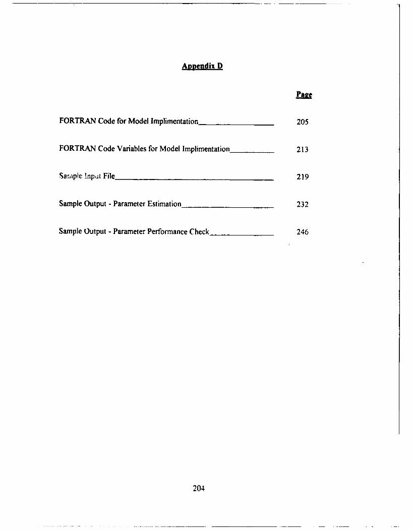
Appendix D

Page

FORTRAN Code for Model Implimentation 205

FORTRAN Code Variables for Model Implimentation 213

Saiple !npJt File 219

Sample Output - Parameter Estimation 232

Sample Output - Parameter Performance Check 246

204

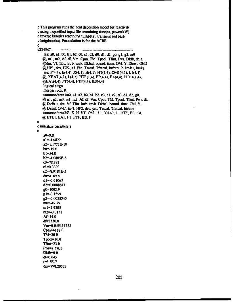
c This program runs the heat deposition model for reactivityc using a specified input rile containing time(s), power(kW)c inverse kintwics reactivity(niillibeta). transient rod bankc heigth(units). Formulation is for the ACRR-cc234567

real A, al, bO, bi, b2. cO, ci, c2, dO, dl. d-7, gO. gi. g2, mOCa, mlI, m2, Af. df. Vm. Cpm. TM, Tpool. Tfint. PNT, Dklb, dt. t.(a dm, Vf, Thu. htrb. in-.k, Dkbal, bound. time, OM, Y. Dkest, 0M27&,HBPI, dev, HP2, a2, Pin, Tmcal, Tfmcal, hiibint, b, invkl, invksreal F(4,4). E(4.4). X(4,.1), H(4, 1), HT(1,4), OM 1(4, 1), LI1(4. 1)@, XHAT(4, 1), L(4, 1). HTE(l ,4), EP(4,4), EA(4,4). HTE 1(1,4),(gEAI(4.4). F7(4.4). FTF(4,4), BB(4.4)logical alignInteger rods, Rcommordarealla0, al, a2. bO. bl. b2. cO, ci, c2. dD. dl. d'2. go.@gi. g2. mO, ml, m2, Af. df.Vm Cpm, TM, Tpool, Tfint, NaT, dL

4 Dkfb. L. dmn. Wf Tfkrn htrb. invk. Dkbal. bound. time. OM. Y.Ca Dkest, 0M-7, 1HP1. HP2. dev, pin, Tmcal, Tfmcal. htrbintcommon/area2/E. XILi HT. OMI1, LI1. XHAT. L. HTE, EP. EA.(d- HTE 1. EA. 1,TF, FTF, BB. F

Cc initialize parametersc

aO=-9.8al=-4.0822a2=1. 1773E-I0W=-l 9.0bl=54.8b2=-4.0805E-8cO=78.38 Icl=0.3393c2=-8.9181E-5dO=4189.8dl =-O.61063d2=0.0088811IgO=1002.9gI=-0. 1599g2=-0.0028345mD=-49.79mI=2.9305m2=-0.0151Af= 14.0df--3530.0Vm-0.04-5434752Cpm=4182.0TM=20.0Tpool=20.0Tflnt-23.0Pwr-2.57E3Dkfb-.0dz=O.045t='6.3E-7dm=-998.20323

205

Vf-O.09866089TfmnTfirnhtzb=3003.0htubint-=3003 .0invk-'0.0Dkbal-0.0align.false.bound=0.02b-tbound£ime=0.0F( 1, 1)1I-Af~dt*(W IE.1+2.O*bl* 1E4*Tfmn+3.0*b2Tfmn*2)/(df*Vf)

@4Af~d1Tm*(bl IE-4+2.0Ob2*Tfiu)I(dfPVf)+t(1-t)*Pwr*(al*[email protected]*a2*Tfmn)/(df* Vf)F( I,2)-Af~dt* lE-1 *(Tm-Tfin)I(df*Vf)F( 1,3)=Af~dt*IE~4(Tm*Tfm.-Tfm**2)/(dt*Vf)

F(2, 1)=0.0F(2,2)=I .0F(2,3)=0.OF(2.4)=O 0F(3, 1)=0.OF(3.2)=0.0F(3.3)=1.0F(3 .4)=0.0F(4. 1)=0.0F(4,2)=0.0F(4,3)=0.0F(4.4)=1 .0call Transmnat(F.FT1,4.4)call Matmuh(FT.4,4,F,4,4.FTF)E(l, 1)= 1.0E( 1.2)=0.000 IE(I.3)=0.000025E(l.4)=-0.000042E(2, 1)=0.0001IE(2.2)= 1.0E(2.3)=0.0E(2.4)=0.0E(3. 1)=0.000025E(3,2)=0.0E(3,3)1I.0E(3,4)-0.OE(4, 1)O..000043E(412)-0.0E(4,3)0O.0E(4,4)=1 .0invk I-invk

100 invkreinvk 1+invk)/2.0Dkest-validate(invk., invks, Dkbal.b)prnt*, time. Dkest. TfmnIF (align) THEN

call Estmodelend iFcall Ad%7nodel

206

Dkb~ractfbTMM,Tfint)Read *, time, Pin. R.. rodsPwr--Pin 1E3invkl~im'kinvk--rea(R)*0.001btib-real(rods)Dkbal=Dkdb-reactr(htrb)/lO0.0+reactr(htrbint)/100.000TO0100

1000 endc

subroutine Advmodel

cornmon/areal/aO, al, a2, WO, bi, b2, co, ci, c2, do, dl, d2, gO,@ gi, g2, mo, ml.. m2, Af, dr, yin. Cpmn. TM. Tpool, Thint, PNT, dL,@ Dkfb, t, din, Vf, Thu htub, invk, Dkbal, bound, time, OM4, Y,@ Dkest, 0M2, HP1, HP2, dev, pin., Tmcal., Tfmncal. htrbintcommnon/area2/E(4..4). X(4. 1). H(4.I1). HT(l.4). OMJ1(4,I1). L 1(4, 1)

@gEAI(4,4), FT(4,4). FTF(4,4), BB(4,4). F(4,4)

Tfincal=Tfi11-Afdt*(b0* 1E-l *Tfin+bl * E.4*Tfin**2+b2*Tfmn*3)/(df*Vt)@+Af~dt*Tm*(W 1IE-1 4bl *lE4*Tfi1~b2*Tfmn**2)I(df*Vf.( I -t)*d*Pw-r*@(a01IE-4+a1* 1E4*Tfrn+a2*Tfm**2)/(df* Vt)

c Tinca1=Tmn.dt*(Af1NcO+c ITfiu+c2*Tfm**2)*(Tfin-Tm)+Plr4 t-(m0+m I Tm+c @m2*Tm**2)*(dO+dl *Tm+d2*Tm**2)*2.0*(Tm.Tpool))/((go+gl *Tm+g2*c @Tm**2)*(dO+dI *Tm+d2*Tm**2)*Vm)

F(I, l)=1-Af~dt*(b0* E1+2.0*bl*le-4Tfm+3 .0*b2*Tfmn*2)/(dfWOf+@A1fIdt*Tm*(bl*IE.4+2.0*b2*Tfin)/(df*Vf)+dt*( I-t)*Pwr(al * E-7+2.0@*a2*Tfmn)/(df*WI)F(1,2)=Af*dl 1E-1*(Tm-Tfmn)/(df*Vf)F( 1,3)=Af~dt* 1E-4(Tm*TfTn.Tfm**2)/(df*Vt)F( 1,4)=( I 4)Pwr~dt 1E-41(df VI)H( 1,1 )=(-3.85+730.O*Tfmn/(273. 15+Tfmn)**2.730.0I(273. 15+Tfrn)[email protected]/(2 73.1 S+Tfin)**2)* IE-S/0. 0073

call Matmult(HT, 1 ,4EA44,HTE)call Matmult(HTE. l.4,R4. 1HPI)HP2=-l .0/(HP1+1E-7)call Multscale(HTE,HTE 1,HP2. 1.4)call Matmnult(H,4, I HTE1, 1,4,EP)call Matrnult(E,4,4,EP,4,4,EA)call Addmat(E,EAEAI ,4,4)call Transmat(F,Fr,4,4)call Matmuit(EAI,4,4,FI',4,4,FTFcall Matinult(F,4,4,FTF,4,4,E)Tfin-Tfmcal

c Tm=TmalWreturnend

cc

subroutine Estmodelc

207

cornmoa/areal/aO, al, a2, bO, bi. b2, cO, cl. c2. dO, dl, d. SO.(g gI, g2, mO, mlI, ra2. Af df, Vra, CpM Th4 Tpool, Tfint, Ny., dt,

SDk~b. t. dni, Vf~ Tftn, hurb, im'k, Dkbul, bo4untme, CM. Y,@ Dkest, 0M2. BPI, HP2, dev, pin. Tracal. Tfhwca. htzbintcwomron/area2/E(44), X(4,1), H(4,l1), HT(l,4), OMI(4,l1), Ll1(4,l1)

@EAl(4,4), FT(4.4), FTF(4.4), BB(4,4), F(4,4)c

X(I.I)=TfmnX(2, 1)=bOX(3,I)=blX(4, 1)-aOH( 1,1 )=(-3.85+730.0*Tfn/(273. 15+Tfm)**2-730.0/(273.l S+Tftn)[email protected]*Tfint/(273. 15+Tfmn)*2)* IE-S/0.0073

H(2,1)=0.OH(3,l)=0.0H(4.l)=0.OY=Dkest+reactr(htub)/l00.O-reactr(htrbint)/IO0.0HT( 1,2)=O.OHT( 1,3)=O.0HT( I.4)0O.Ocall Matmault(E.4.4.H,4. I OM 1)call Matrnuil(HT, I .4OM 1,4. L OM)OM=OM+ IE-70M2=1.0/OMcall Multscale(QM 1 .L.0M2,4., 1)dev--(Y-(Tfmn-Tfint)*(-3.85-(730.0/(273.1I5+Tfmn)))1IE-5/O.0073)call Multscale(L.LlI~ev.4, 1)call Addmnat(XL I ,XHAT,4. 1)Tfin=XHAT(l 1,)W=-XHAT(2. I)bi =XHAT(3. 1)aO=XHAT(4j )returnend

C

csubroutine Addmat(A.B,C.N,M)

CInteger N,MKijreal A(N,,M). B(N,M). C(N.Mf)Do 10, i-I,NDo 10, j1 ,M

10 CQij)ýA(ij)+B(ij)returnend

cC

subroutine Transmat(A.C.N.M)C

Integer N.Mijreal A(N.M). C(N.M)Do 20, i=1.N

208

Do 20. j= IM20 C(ij)=A(j.i)

returnend

c

Csubroutine Multscale(A.C,b,N,M)

Integer N,,i jreal A(N,M), C(N,M). bDo 30, i=-.N

Do 30, j=I.M30 C(ij)=b*A(ij)

returnend

C

subroutine Matmult(A.N.M.B.M.k.C)c

Integer i.j.w.N.M.kreal A(N,M). B(Mk). C(NAk). sumDo 50, i=l.N

do 50. j=l.ksum=0.0Do 40. %-- I,M

sum=sum+A(i.w)*B(wj)40 continue

C(ij)=sum50 continue

returnend

C

real function reactr(p)c

real pif(p.It. 2031.) p=203 1.if(p .gt. 7460.) p=7460.if(p .le. 2700.) go to 600if(p .le. 3100.) go to 605if(p .le. 3300.) go to 610if(p .le. 3500.) go to 615if(p .le. 3700.) go to 620if(p .le. 3900.) go to 625if(p .le. 4100.) go to 630if(p .le. 4300.) go to 635if(p .le. 4500.) go to 640if(p .le. 4700.) go to 645if(p .le. 4900.) go to 650if(p .le. 5100.) go to 655if(p .le. 5300.) go to 660if(p .le. 5500.) go to 665if(p .le. 5700.) go to 670

209

if(p .le. 5900.) go to 675iI~p.le. 6100.) go to 680if~p .le. 6300.) go to 685ift .le. 6700.) go to 690if~p .le. 7 100.) go to 695if(p kc. 7500.) go to 700go to 705

600 reactr=-0.016143*p+472.98S693return

605 feactr--0.049250*p+-6 2.375return

610 mcreac=.0.0765*p+-646.85return

615 reactr-O-.O9 1 "94.7return

620 reactr=-0. 1005 p+727.9return

625 reactr-O-.1085*p+757.5return

630 reactr-=.0.1225*p+812.15return

635 reactr-.0.125*p+822.4return

640 reactr-0-. 1305*p+846.05return

645 reactr--0.1295*p+841.55return

650 reactr=.0.1295OP4g41.5return

655 reactr=-O.122*p+8o4.8return

660 reactr=0-. 12O*p+ 794.6return

665 reactr=-0.1I10*p474 1.6return

670 reactr--0.1065*p-'722,35return

675 reactr---0.0965*p+665.35return

680 reactr=-0.097*p+668.3veturn

685 reactr-.0.076*p+540,2retur

690 reactr--0.0657S*p+475.625return

695 reactr,-0.04725*p435 1.675return

700 reactr--0.028*p+2 15.0retur

705 reactr-0.00333*p+30.0returnend

c

c

210

real function reactfb(T.TIN)c

real T,TIN.TKTK=T+273. 15reactfb=(T-TlN)*(-3.85-730.0ITK)* 1E-5/0.0073returnend

cC

real function validate(majb.mc~b)c

real m(3), N(3), PAR. TEST. m'2(2), N2(2),breal ma~mb.mcinteger i,km(l)=rnam(2)=mbm(3)=mcDo 10. i=1.3

N(i)=ABS(ni(i)-(m( 1)+m(2)+m(3 ))13 .0)10 continue

TEST=(8.0/3.0)*((m(1)*b)**2)PA.R=abs(N( 1)**2+N(2)**2-+N(3 )**2..-(9.0*N( 1)**2)12.0)if(PAR .lt. TEST) THEN

validate-(m(]I)+m(2)+m(3))/3.0go t 100

end ifif(N(1) .gt. N(2)) THEN

if(N(l) .gt. N(3)) THENm2(1)=m(2)mi2(2)=rn(3)

elsem2(l)=m(1)m2(2)=m(2)

end ifelse

if(N(2) .gt. N(3)) THENm2(1)=m(l)m2(2)=m(3)

elsem2(1)=m(1)m2(2)-m(2)

end ifend ifDo 40, k= 1,2

N2(k)=abs(m2(k)-(m2(1I)+m2(2))/2.0)40 continue

TESTh2.0*((b~m(1))**2)PAR--abs(N2(1I)**2+N2(2)**24..0*N2(1I)'*2)if(PAR .lt. TEST) THEN

validate=(m2( 1)+m2(2))/2.0go to 100

elsev*Alidate--m( I)

end if

211

00returnend

212

FORTRAN Code Variables for Model mnolimentation

ao, aI, a2 Polynomial coefficient for a second order polynomialrepresnting the inverse

of the fuel specific heat capacity.

bo, b1, b2 Polynomial coefficients for a second order Polynomial representing the

overall fuel to coolant heat transfer coefficient divided by the fuel specific

heat capacity.

Co, C 1 , C2 Polynomial coefficients for a second order Polynomial representing the

overall fuel to coolant heat transfer coefficient.

do, d I, d2 Polynomial coefficients for a second order polynomial the moderator

specific heat capacity.

go,, g 2 Polynomial coefficients for a second order polynomial representing the

moderator density (Main, Advmodel, Estmodel).

mo, mIn, m2 Polynomial coefficients for a second order polynomial representing the

moderator mass flow rate.

Af fuel to coolant heat transfer surface area.

lf fuel density

213

Vm Volume of moderator within the core.

Cpm Specific heat capacity of moderator.

Tm Moderator average temperature.

Tpool Reactor pool temperature.

Tfint Initial fuel temperature.

PWR Reactor Power.

DKfb Thermal feedback reactivity.

dt Sample time.

t Percentage of fission power deposition in the coolant due to gamma

heating.

Vf Fuel volume.

Tfmn Fuel temperature as perdicted by thermal model.

214

htrb Transient rod bank position.

invk Reactivity calculated via Inverse Kinetics.

DKbal Reactivity calculated via reactivity balance.

bound Percentage error bound of reactivity signals for use in signal validation.

time Elapsed time since start of transient.

OM Value used in calculation of estimation routine Kalman gain.

Y Estimation routine value of actual reactor reactivity equal to the validated

reactivity signal.

DKest Value of the validated reacivity signal.

dev Estimation routine value of innovation equal to the difference between

actual and estimated reactivity.

Pin Initial reactor power.

Tmcal Perdicted moderator temperature for next time step.

215

htrbint Initial position of transient rod bank.

b Percentage error bound of reactivity signals for use in signal validation.

lnvkl Inverse Kinetics reactivity from previous step inverse kinetics reactivity.

F Linearized system matrix for model parameter estimation.

Ft Transpose of matrix F.

E System error covariance matrix for model parameter estimation.

X Present value of model fuel temperature, and model thermal parameter

coefficients bo, b1, and ao.

H System descriptive matrix.

HT Transpose of matrix H.

R Interger value of input inverse kinetics reactivity as read from input file.

XHAT Estimation values of fuel temperature, and model thermal parameter

coefficients, bo, b1, ao.

216

L Matrix representing Kalman estimation gain.

Align Logical varible used to determine it estimation routine should be used.

True = Estimate new model parameter coefficients.

False = Use present values of model coefficients.

A,B,C,N,M Matrix values used in matrix math routines.

p Dummy variable for transient rod position in reactivity function reactor.

T Dummy variable for fuel temperature in reactivity function reacfb.

Tin Dummy variable for initial fuel temperature in reactivity function reacfb.

TK Fuel temperature ('K)

Ma, Mb, Mc Measured reactivity values in reacivity validation routine.

PAR Value of parity vector magnitude for a reactivity measurement.

Test Consisting threshold for parity test during reactivity signal validation.

217

M(I),M(2),M(3) Measured reactivity values in reacivity validation routine.

OM2, BPI, HP2, HTE, EP, EA, HTE, EAI, FTF, BB are scalar and matrix variables used

as intermediate values during parameter calculation.

218

0.04 2.70 25 30040.09 2.80 50 30050.13 2.93 127 30060.17 3.02 149 30250.22 2.58 -16 30820.25 2.59 -1 31020.3 3.5 277 31290.33 3.12 156 31540.38 3.23 195 31540.42 3.22 185 31660.47 3.11 153 31900.5 3.48 254 32250.53 3.72 295 32550.58 2.97 90 32890.63 4.99 492 33190.67 3.83 267 33460.7 4.08 341 33440.75 3.89 296 33590.8 3.85 286 33880.83 5.65 543 34180.87 4.48 352 34430.92 4.39 358 34450.97 4.26 331 34571 4.28 332 34871.05 4.74 401 35171.08 5.43 480 35491.13 6.51 562 35931.17 6.14 510 36131.22 6.77 562 36421.25 6.48 522 36751.3 7.67 605 37041.33 8.49 636 37361.38 9.69 675 37661.42 8.86 615 37981.47 10.83 698 38321.5 11.3 694 38651.55 12.24 712 38991.58 13.59 736 39291.63 17.37 794 39711.68 22.23 833 39831.72 21.48 796 40001.77 27.27 848 40081.8 29.05 838 40151.85 34.5 861 40201.88 31.1 809 40231.93 35.06 838 40271.98 42.63 862 40352.02 43.36 842 40372.07 52.93 873 40422.1 58.63 873 40452.15 57.39 849 40472.18 68.13 878 40422.23 64.7 842 40272.27 74.12 865 4043

219

2.32 82.38 866 40402.35 87.86 862 40302.4 88.8 849 40352.45 95.71 852 40352.48 107.16 863 40302.53 118.76 865 40302.58 106.9 821 40302.62 117.27 840 40252.67 120.83 831 40272.7 122.16 820 40252.75 147.35 854 40272.8 164.99 857 40322.83 166.14 839 40302.88 181.68 850 40302.92 200.95 857 40182.97 197.24 835 40253.02 230.9 859 40233.05 193.27 786 40253.1 223.55 833 40253.13 239.3 832 40253.18 271.69 847 40253.23 288.01 841 40273.27 328.78 859 40303.32 354.94 855 40303.35 390.74 862 40353.4 370.11 832 40303.45 432.1 857 40303.48 436.49 838 40303.53 482.29 851 40323.57 483.75 834 40323.62 447.24 805 40253.67 508.3 831 40233.7 595.81 854 40373.75 582.91 827 40353.78 717.44 868 40373.83 739.89 849 40373.88 779.94 846 40373.92 818 842 40353.97 882.66 847 40374 837.31 815 40374.05 973.96 848 40404.1 1062.97 847 40354.13 1051.06 826 40404.18 1135.26 837 40454.23 1307.45 853 40424.27 1407.67 851 40474.32 1436.18841 40454.37 1436.59 827 40454.4 1538.31 833 40424,45 1649.69 835 40474.5 1733.55 831 40504.53 1998.42 854 40524.58 2010.3 834 40604.63 2107.71 832 4055

220

4.67 2305.83 841 40604.72 2387.47 833 40604.77 2579.94 837 40674.8 2659.68 829 40674.85 2851.86 835 40674.9 3021.09832 40694.93 31%.9 832 40724.98 3358.07 831 40745.03 3497.26 826 40775.07 3570.52 817 40745.12 3651.1 813 40745.17 3687.73 803 40725.2 3717.03 793 40645.25 3746.33 788 40645.28 3775.64 779 40605.33 3826.92 776 40625.38 3922.15 772 40525.42 3980.76 766 40625.47 4039.36 762 40625.5 4046.69 753 40605.55 4090.64 750 40605.58 4083.32 739 40555.63 4105.29 735 40555.68 4127.27 728 40555.72 4163.9 723 40555.77 4149.25 715 40525.8 4200.53 712 40505.85 4163.9 703 40505.88 4149.25 694 40455.93 4149.25690 40475.98 4149.25 683 40476.02 4149.25 676 40426.07 4134.6 670 40476.1 4127.27 662 40426.15 4119.94 658 40426.2 4083.32 648 40376.23 4083.32 642 40356.28 4039.36 634 40326.33 4039.36 629 40326.37 4002.73 619 40306.42 3973.43 613 40276.45 3973.43 608 40306.5 3980.76 606 40326.55 4017.38 605 40306.58 3995.41 597 40326.63 3973.43 591 40306.67 3973.43 587 40306.72 3973.43 584 40326.77 3973.43 579 40306.8 3966.1 574 40326.85 3988.08 574 40326.88 3958.78 565 40326.93 3929.48 559 40276.97 3922.15 554 4025

221

7.02 3922.15 552 40327.07 3944.13 551 40357.1 3966.1 550 40377.15 3958.78545 40407.18 3966.1 543 40407.23 3995.41 544 40527.28 3995.41 539 40457.32 3995.41 535 40457.37 4017.38 535 40477.4 3988.08 527 40507.45 3973.43 523 40477.5 4002.73 524 40507.53 4002.73 519 40557.58 4010.06 518 40577.63 4010.06 514 40557.67 4010.06 510 40577.72 4039.36 512 40627.75 4002.73 503 40627.8 4017.38 503 40727.83 4002.73 497 40697.88 3988.08 493 40727.93 3988.08 490 40697.97 3988.08 487 40678.02 3980.76 484 40678.07 3980.76 481 40698.1 3995.41 480 40728.15 3995.41 478 40698.18 3988.08 473 40778.23 4002.73 474 40778.28 3995.41 469 40738.32 3995.41 466 40798.37 4017.38 468 40828.4 3980.76 459 40778.45 3973.43 456 40848.48 3958.78 451 40848.53 3958.78 450 40928.58 3973.43 450 40878.62 3966.1 445 40898.67 4010.06 451 40928.7 3951.45 438 40928.75 4002.73445 40978.8 3973.43 437 40998.83 3951.45 431 41028.88 3966.1 433 41048.93 3995.41 435 41028.97 3966.1 427 41069.02 3980.76428 41099.05 3958.78422 41119.1 3966.1 422 41139.13 3944.13416 41169.18 3951.45 416 41169.23 3973.43 417 41199.27 3973.43 414 41269.32 3995.41 416 4126

222

9.35 3958.78407 41269.4 3966.1 408 41299.45 3966.1 406 41319.48 3980.76406 41349.53 3980.76404 41369.58 3951.45 397 41369.62 3944.13 394 41399.67 3951.45 394 41319.7 3966.1 394 41439.75 3951.45 390 41489.78 3922.15 383 41519.83 3958.78 389 41519.88 3980.76390 41519.92 3980.76 388 41589.97 4002.73 390 416310 4002.73 388 416610.05 3988.08 384 416810.1 4024.71 388 417110.13 4002.73 381 417310.18 3995.41 379 417310.23 3980.76 375 417610.27 3973.43 372 417610.32 3966.1 369 417310.35 3973.43 369 418310.4 3936.8 361 418810.45 3966.1 365 419310.48 3980.76 366 419010.53 3973.43 363 419510.57 3973.43 361 419810.62 3944.13 355 419810.67 3951.45 355 420310.7 3980.76 359 420510.75 3973.43 356 421010.8 3973.43 354 420510.83 3980.76 354 421310.88 3980.76352 421810.92 3980.76 351 422010.97 3951.45 344 422011.02 3973.43 347 422511.05 3988.08348 421811.1 3980.76345 423211.15 3980.76344 424511.18 3988.08343 423711.23 3995.41 344 424011.27 3988.08 340 424511.32 3980.76338 424211.37 3988.08 338 425011.4 3988.08 336 425211.45 3988.08335 425511.5 4032.04 342 425711.53 4010.06335 425711.58 3988.08 331 426211.62 3988.08 330 426711.67 4002.73 331 4262

223

11.72 4032.04 335 427411.75 4002.73 327 426511.8 4032.04332 427411.85 3995.41 324 428211.88 4010.06326 428211.93 3995.41 321 429211.97 3995.41 320 429212.02 4024.71 325 429212.07 4010.06320 429612.1 3995.41 316 429612.15 3988.08 314 430112.18 3995.41 315 430412.23 3966.1 308 430612.28 4010.06316 431112.32 4002.73 312 431412.37 4002.73 311 431412.42 3995.41 309 431912.45 3980.76 305 432412.5 3980.76 304 432412.55 3958.78 299 432912.58 3988.08 304 433112.63 3980.76 301 433812.67 3973.43 299 433612.72 3995.41 302 434612.77 3995.41 301 434112.8 3995.41 299 434812.85 3988.08 297 434812.88 3988.08 296 435312.93 3988.08 295 435612.98 4002.73 297 436113.02 4002.73 296 436613.07 4002.73 295 436813.12 4002.73 294 437113.15 3995.41 291 437313.2 3995.41 291 437813.25 4017.38 294 438013.28 3995.41 288 438513.33 4002.73 289 438813.37 3988.08 285 439013.42 3944.13 276 439513.47 3995.41 286 439313.5 4010.06 287 440013.55 4002.73 284 440813.58 4002.73 283 441013.63 3995.41 281 441013.68 3980.76 277 441513.72 4010.06 283 441513.77 4010.06281 442013.82 4017.38 282 442513.85 4002.73 277 442513.9 3995.41 276 442513.93 4002.73 276 443213.98 4002.73 275 443014.03 4010.06 276 4440

224

14.07 4010.06 275 444214.12 3988.08 270 444514.17 3980.76268 444714.2 4002.73 272 445214.25 4002.73 270 445414.3 4017.38272 446214.33 4046.69 277 446214.38 3995.41 266 446414.42 3995.41 265 446414.47 3995.41 265 446214.52 4010.06 267 447214.55 3995.41 263 447714.6 3980.76 259 447714.65 3995.41 262 447714.68 3995.41 261 448414.73 3980.76 257 448914.77 4002.73 261 449114.82 4010.06 262 449614.87 4010.06 261 449914.9 4002.73 258 450614.95 4024.71 262 450615 4010.06 258 450915.03 3995.41 254 450915.08 4002.73256 451415.12 4017.38 258 451615.17 3995.41 252 451615.22 3995.41 252 452415.25 3995.41 251 452815.3 4010.06 254 452815.35 4002.73 251 453315.38 4017.38 253 453615.43 3995.41 248 453815.47 3980.76244 454115.52 3958.78 240 454615.57 4002.73 249 454815.6 4002.73 247 455315.65 4017.38250 455815.7 4010.06 247 456115.73 3966.1 237 456315.78 4002.73 245 456315.83 4010.06 245 457015.87 3995.41 241 457315.92 4002.73 243 457315.97 4010.06 243 457516 4010.06 243 458016.05 4010.06 242 458316.1 4010.06 241 458816.13 4002.73 239 459016.18 3995.41 237 459316.22 3973.43 232 459816.27 3988.08 235 460016.32 4017.38 240 460516.35 4010.06 237 460716.4 4017.38 239 4610

225

16.45 4017.38238 461716.48 4002.73234 461516.53 3980.76229 461516.58 3980.76229 462016.62 3988.08 230 462516.67 4002.73 232 462516.72 4002.73 232 463016.75 3995.41 229 462216.8 3995.41 229 463716.85 4017.38 233 464216.88 4010.06 230 464416.93 3988.08 225 464416.97 4010.06 230 464917.02 4017.38 231 465217.07 4010.06 228 465917.1 4010.06 228 465917.15 4002.73226 466217.2 4024.71 230 466417.23 4024.71 229 466917.28 4024.71 228 467217.33 4010.06 224 467717.37 4010.06 224 467717.42 4010.06 224 467917.47 4017.38 224 468417.5 3995.41 219 468617.55 4002.73221 468917.6 4002.73 220 469417.63 4010.06 221 469617.68 4010.06 220 469617.72 3995.41 217 469617.77 3995.41 217 469917.82 4002.73 218 470617.85 3988.08214 470417.9 3995.41 215 471117.95 4002.73 216 471417.98 3966.1 207 471618.03 4002.73 216 471618.08 3988.08 212 472618.12 3988.08211 472318.17 3988.08 211 472618.22 4002.73214 472618.25 3988.08210 473618.3 3988.08 210 473618.35 4010.06 214 473818.38 4017.38 214 473318.43 4010.06 212 474618.47 4010.06 212 474618.52 4010.06 211 475118.57 4002.73 209 474618.6 3995.41 207 475818.65 4017.38 212 476118.7 4024.71 212 475318.73 4039.36 215 476518.78 4032.04213 4768

226

18.83 4024.71 210 477018.87 4024.71 210 477518.92 4032.04211 477518.97 4039.36212 477819 4017.38206 478019.05 4010.06 205 478019.08 4002.73 203 478019.13 3995.41 201 478519.18 4010.06204 478819.22 4010.06203 479019.27 4002.73 201 479519.32 4024.71 206 479519.35 4010.06 202 479819.4 4017.38 203 480019.45 4010.06 201 481019.48 4010.06201 480519.53 4017.38 202 480719.58 4010.06200 481019.62 4010.06 199 481219.67 4010.06 199 481519.72 4024.71 202 482019.75 4010.06 198 482219.8 4024.71 201 482219.83 4039.36 203 482719.88 4039.36 203 482719.93 4054.01 205 483219.97 4046.69203 483520.02 4039.36 201 483520.07 4039.36 200 483520.1 4024.71 196 483720.15 4039.36 200 484220.2 4024.71 196 484420.23 4032.04 197 484420.28 4046.69 200 484920.33 4010.06 191 484920.37 4024.71 194 485220.42 4024.71 194 485420.47 4010.06 190 484920.5 4010.06 190 485720.55 4024.71 193 485920.58 4039.36 1% 486220.63 4039.36 195 486420.68 4046.69 1% 486720.72 4075.99 202 486720.77 3988.08 181 486920.82 3973.43 179 486920.85 3966.1 178 486720.9 3988.08 183 486920.93 3980.76 180 487220.98 3980.76 180 487921.03 4010.06 186 487921.07 3980.76 179 487921.12 3995.41 183 489421.17 3966.1 176 4881

227

21.2 3966.1 176 488921.25 3944.13 171 488921.28 3980.76 180 488921.33 3995.41 182 489121.38 4002.73 183 489921.42 3988.08 179 490121.47 3973.43 176 489621.52 3973.43 176 490621.55 3966.1 174 490621.6 3995.41 180 490621.65 3980.76 176 490621.68 3988.08 178 491421.73 3980.76 176 491421.78 4024.71 185 491821.82 4010.06 181 492121.87 4024.71 184 492321.9 4002.73 178 492321.95 4010.06 180 492622 4010.06 180 493122.03 4010.06 179 493322.08 4017.38 180 493322.13 4010.06 178 493622.17 3995.41 175 493622.22 4017.38 180 493822.25 4002.73 175 494122.3 4010.06 177 494122.35 4024.71 180 494622.38 4010.06 176 494822.43 4010.06 176 494822.48 3980.76 169 495122.52 3995.41 173 495122.57 3980.76 169 495522.62 3995.41 172 495822.65 4010.06 175 496022.7 4010.06 174 496022.75 3995.41 171 496322.78 3995.41 170 496322.83 4024.71 177 496522.87 4002.73 171 496822.92 4010.06 173 497022.97 3980.76 166 497323 3995.41 169 497323.05 4002.73 170 497823.1 4002.73 170 497823.13 3966.1 161 498323.18 4002.73 170 498323.22 3995.41 167 498523.27 3995.41 167 499023.32 4032.04 175 499023.35 3995.41 166 499323.4 3988.08 165 498323.45 3995.41 166 499723.48 3980.76 162 499023.53 3988.08 164 5000

228

23.58 3995.41 165 501523.62 4002.73 167 500523.67 3988.08 163 500523.7 3980.76 161 500723.75 3995.41 165 501223.8 3980.76 161 501523.83 3988.08 162 501523.88 3995.41 164 501723.93 3980.76 160 502023.97 3995.41 163 502224.02 3995.41 163 502524.07 3988.08 161 503024.1 4002.73 164 503224.15 4010.06 165 503724.18 4002.73 163 503424.23 4002.73 163 504924.28 4017.38 166 504224.32 3988.08 158 503924.37 4002.73 162 504724.42 4002.73 162 504724.45 4002.73 161 504924.5 3995.41 159 504924.55 4002.73 161 505424.58 3988.08 157 505724.63 3995.41 159 505724.68 3951.45 148 505924.72 3980.76 156 506224.77 3973.43 153 506224.8 3988.08 157 506724.85 3995.41 158 506724.9 3988.08 156 507924.93 3995.41 157 507624.98 3995.41 157 507425.03 3995.41 157 507925.07 4039.36 167 508125.12 4010.06 159 508625.17 3995.41 155 508425.2 3980.76 152 508625.25 4010.06 159 508625.28 3995.41 154 508125.33 3980.76 151 509125.38 4002.73 156 509625.42 3980.76 150 509625.47 4002.73 156 510125.5 4010.06 157 510125.55 3995.41 153 510625.6 3973.43 148 510925.63 3973.43 148 511125.68 4010.06 156 511325.73 4010.06 156 511625.77 4002.73 153 510425.82 4010.06 155 511825.87 4002.73 153 512325.9 4010.06 154 5126

229

25.95 3973.43 146 512826 4002.73 153 513126.03 3995.41 150 513326.08 4010.06 154 513626.13 4032.04 158 513626.17 4010.06 152 514126.22 4032.04 157 514626.25 4010.06 152 514326.3 4010.06 152 514626.35 4017.38 153 515026.38 4010.06 151 515326.43 4002.73 149 515326.48 3995.41 147 515526.52 4002.73 149 515826.57 4010.06 150 516026.62 4032.04 155 516326.65 4017.38 151 516526.7 3988.08 144 516826.73 4002.73 148 516326.78 3995.41 146 517526.83 4039.36 156 517326.87 4024.71 151 517826.92 4024.71 151 517826.97 4002.73 146 518027 4017.38 149 518027.05 4002.73 145 518027.1 4010.06 147 518327.13 4002.73 145 519027.18 4002.73 145 518727.22 3995.41 143 518727.27 4002.73 145 518727.32 3995.41 143 519227.35 4017.38 148 519727.4 4024.71 149 520027.45 3995.41 141 520027.48 3995.41 142 520227.53 3995.41 142 520527.58 4039.36 151 520227.62 3980.76 136 520727.67 3973.43 136 520727.7 3973.43 136 520527.75 3966.1 134 521027.8 3958.78 132 521027.85 3973.43 136 521527.88 3958.78 132 522027.93 3958.78 132 522027.97 3966.1 134 522528.02 3944.13 129 522728.07 3973.43 136 522728.1 3980.76 137 523428.15 3995.41 140 523428.2 4024.71 146 523428.23 3973.43 133 523728.28 3973.43 134 5239

230

28.32 3951.45 129 524228.37 3980.76 136 525928.42 3973.43 134 524928.45 3966.1 132 525228.5 4002.73 141 525428.55 3995.41 138 525928.58 3966.1 131 525928.63 3988.08 137 525928.67 3988.08 136 526228.72 3980.76 134 527428.77 4010.06 141 526928.8 4017.38 142 525928.85 4002.73 138 527428.9 3995.41 136 527628.93 4024.71 143 527628.98 4002.73 137 528429.03 4024.71 142 528429.07 4024.71 141 528629.12 4032.04 143 528129.17 4010.06 137 529129.2 4032.04 143 529429.25 4046.69 145 529929.28 4032.04 141 530129.33 4039.36 143 530129.38 4046.69 144 530329.42 4046.69 143 530629.47 4046.69 143 530829.52 4039.36 141 531329.55 4024.71 137 531129.6 4024.71 137 531629.65 4010.06 134 531829.68 4032.04 139 531629.73 4010.06 133 532129.78 4032.04 138 532129.82 4061.34 145 532129.87 4017.38 134 532629.9 4032.04 137 532629.95 3980.76 125 533130 4017.38 134 5333

231

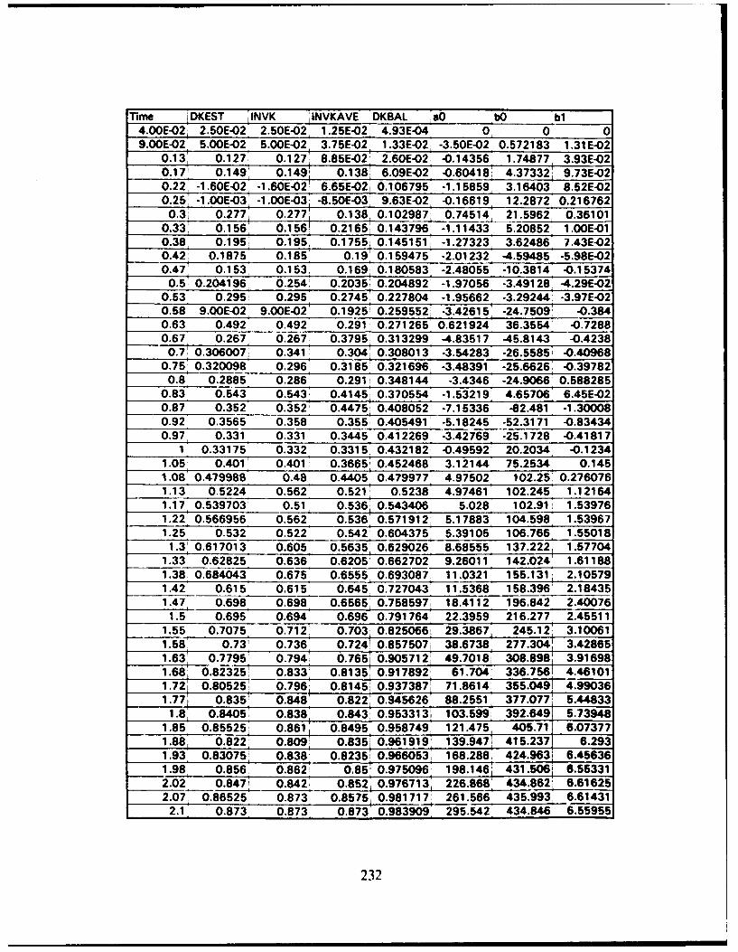
Time I DKEST INVK INVKAVE DKBAL &a0 bO bl4.OOE`02i 2.50E-02 2.50E-02, 1.25E-02 4.93E-04 0. 0 09.OOE-02 5.OOE-02 5.OOE`02 3.75E-02, 1.33E-02, -3.50E-02 0.572183 1.31E-02

0.13 0.127. 0.127' 8.85E-02 2.60E-02 -0.14356 1.74877 3.93E-020.17 T 0.149' 0.149 0.1381 6.09E.02i -0.60418: 4.37332! 9.73E-020.22 -1.60E-02 -1.6OE-02 6.65E-02Q 0.106795 -1.15859 3.16403 8.52E-020.25 -1.OOE-03 -1.OOE-03 -8.50E-03, 9.63E-02 -0.16619 12.2872 0.2167620.3i 0.277, 0.277 0.138 0.102987, 0.74514; 21.5962, 0.36101

0.33, 0.156, 0.156! 0.2165:' 0.143796 -1.11433 5.20852' 1.OOE-010.38, 0.195, 0.195, 0.1755 0.145151' "1.27323: 3.62486 7.43E-020.42 0.1875 0.185 0.19' 0.159475 -2.01232 -4.59485 -5.98E-020.47' 0.153. 0.153, 0.169, 0.180583 -2.48055 -10.3814 -0.153740.5 0.204196 0.254ý 0.2035 0.204892 -1.97056 -3.49128, -4.29E-02

0.53 0.295: 0.295 0.2745' 0.227804 -1.95662 -3.29244 -3.97E-020.58 9.OOE-02 9.OOE-02' 0.19251 0.259552i -3.42615; -24.7509' -0.3840.63 0.492 0.492 0.291 0.271265 0.621924 36.3554 -0.72880.67. 0.267 0.267 0.3795 0.313299 -4.83517 -45.8143 -0.4238

0.7 0.306007' 0.341! 0.304ý 0.308013 -3.54283 -26.55851 -0.409680.75' 0.320098 0.296 0.3185 0.3216964 -3.48391 -25.6626:; -0.39782

0.8 0.2885 0.286 0.291 0.348144 -3.4346' -24.9066 0.5882850.83 0.543 0.543- 0.4145: 0.370554 -1.53219: 4.65706 6.45E-020.87 0.352 0.352 0.4475i 0.408052 -7.15336 -82.481 -1.300080.92 0.3565 0.358 0.355 0.405491 -5.18245 -52.3171 -0.834340.97, 0.331 0.331 0.3445 0.412269 -3.42769 -25.1728 -0.41817

1 0.33175 0.332 0.3315. 0.432182 -0.49592 20.2034 -0.12341.05 0.401! 0.401 0.3665: 0.452468 3.12144 75.2534, 0.1451.08 0.479988 0.48 0.4405 0.479977 4.97502 102.25 0.2760761.13 0.5224 0.562 0.521' 0.5238 4.974611 102.245 1.121641.17 0.539703 0.51 0.536 0.543406 5.028 102.91 1.539761.22 0.566956 0.562 0.536 0.571912: 5.17883, 104.598 1.539671.25 0.532 0.522 0.542 0.604375 5.39105 106.766 1.55018

1.3 0.617013 0.605 0.5635, 0.629026 8.68555 137.222 1.577041.33 0.62825 0.636 0.6205' 0.662702 9.26011 142.024' 1.611881.38 0.684043 0.675 0.6555, 0.693087. 11.03211 155.131; 2.105791.42 0.615 0.615 0.645 0.727043' 11.5368 158.396 2.184351.47 0.698 0.698 0.6565 0.758597. 18.4112 196.842 2.40076

1.5 0.695 0.694 0.696 0.791764, 22.3959 216.277 2.455111.55 0.7075 0.712, 0.703 0.8250661 29.3867, 245.12' 3.100611.581 0.73' 0.736 0.724! 0.8575071 38.6738, 277.3041 3.428651.63.7795' 0.794 0.765i 0.905712; 49.70181 308.898' 3.916981.68 0.82325W 0.8331 0.8135' 0.917892' 61.7041 336.7561 4.461011.721 0.80525' 0.796 0.81451 0.9373871 71.8614, 355.0491 4.990361.77i 0.835! 0.848' 0.8221 0.945626' 88.2551' 377.077 5.44833

1.8 0.8405, 0.838 0.843; 0.9533131 103.5991 392.6491 5.739481.85 0.85525, 0.861' 0.8495 0.958749, 121.475 405.71 6.073771.88, 0.822: 0.809 0.835 0.9619191 139.947; 415.237 6.2931.93' 0.83075, 0.838 0.8235 0.966053: 168.288, 424.9631 6.456361.98 0.856 0.862 0.851 0.975096- 198.1461 431.5061 6.553312.02 0.847 0.842ý 0.852 0.976713ý 226.868 434.862; 6.616252.07. 0.86525 0.873 0.8575, 0.981717 261.566 435.9934 6.61431

2.1, 0.873 0.873 0.873 0.983909 295.542 434.846 6.55955

232

2.15 0.898147, 0.849 0.861 0.984439 331.36 431.717 6.444232.18' 0.87075t 0.878 0.86351 0.976488' 362.081. 427.717: 6.29212.23 0.8511 0.842' 0.86: 0.9551431 402.616, 420.964 6.101252.271 0.85925: 0.865! 0.85351 0.971489! 446.029! 412.446 5.916582.32' 0.865751 0.8661 0.8655! 0.963366; 495.607 401.251; 5.645812.35 i 0.863 0.862! 0.864 0.945989 541.52 389.682! 5.332932.4. 0.883674; 0.849; 0.8555 0.946522. 583.011 378.224 4.9418

2.45! 0.851251 0.8521 0.8505 0.9411431 616.105' 368.291 4.549712.481 0.860251 0.863i 0.8575 0.927359 8665.1481 352.298i 4.167192.53' 0.882776& 0.865' 0.864 0.919327 702.839 338.984 3.836052.58 0.832 0.8211 0.843 0.911764! 723.914 330.9961 3.297792.62: 0.83525 0.84, 0.8305 0.895574 770.814. 312.101 2.840572.672 0.851449 0.8311 0.8355 0.887846! 805.829! 296.628 2.55864

2.7; 0.840655, 0.82 0.8255 0.876465; 826.589, 286.63 1.870132.75' 0.85356 0.854, 0.837 0.869679 846.3871 276.222' 1.27849

2.8: 0.8595321 0.857; 0.85551 0.866096k 854.892' 271.315 0.8755422.83 0.846846 0.839 0.848 0.853537, 858.22, 269.267T 0.4321792.88, 0.846056' 0.85: 0.8445! 0.843669: 861.464' 267.1631 0.2104782.92' 0.84323' 0.857 0.8535; 0.819189' 860.38 267.915i 0.1125372.97! 0.833558, 0.835' 0.8461 0.819673 850.1911 275.394: 0.480793.021 0.83833 0.859 0.847, 0.808991: 844.704 279.586' 0.741548

3.05: 0.7945221 0.786 0.8225 0.803044 834.137i 288.21 1.317863.1 0.801582 0.833 0.8095' 0.793664 836.991 285.828' 1.14686

3.13; 0.816252 0.832 0.8325. 0.784257i 834.679' 288.001; 1.316493.18' 0.821298 0.847' 0.8395 0.777394: 826.342 296475: 2.034153.23 0.8425 0.841 0.844 0.772616 816.063 307.574 3.053653.27 0.82705 0.859 0.85 0.772151: 800.855, 323.9921 4.699043.32 0.856 0.855 0.857' 0.763757, 789.609' 335.806: 5.993813.35 0.86025 0.862 0.8585, 0.765347 770.957, 353.317i 8.13613

3.4. 0.8395 0.832 0.847, 0.753566' 751.588 368.726 10.27843.451 0.817135 0.857! 0.8445. 0.749903 733.346 380.0211 12.13213.48 0.84275 0.838 0.8475' 0.74042 719.381 387.531; 13.56923.53' 0.84775 0.851: 0.8445' 0.738611' 697.095 395.986; 15.66933.57; 0.83825: 0.834 0.8425 0.733298, 672.785' 402.416 17.85413.62! 0.81225, 0.805 0.8195' 0.720564' 648.022 405.534: 19.84273.67' 0.788443 0.831 0.818 0.716329 625.813 406.194 21.5249

3.7! 0.807693 0.854 0.8425; 0.726578 609.016 406.121 22.88463.75 0.83375: 0.827; 0.8405 0.714094, 589.707 404.4911 24.37813.78, 0.85775, 0.868: 0.8475' 0.713435 558.589; 3981531 26.39033.83 0.85375' 0.849 0.8585 0.7076! 519.708, 387.421 28.71593.88 0.84675' 0.846! 0.84751 0.7047111 475.0441 369.893: 30.58463.92 0.843; 0.842, 0.844! 0.700881; 427.86 347.501, 31.983.97 0.845751 0.847i 0.8445 0.7044171 377.503i 320.198, 32.9268

4 0.823i 0.8151 0.831' 0.707322Z 325.005 288.7191 33.38384.05; 0.798422 0.848 0.8315| 0.715767; 280.128' 259.354 33.2614

4.1 0.84725 0.847 0.84751 0.708246i 248.4041 237.452! 32.9544.13 0.83125 0.826 0.83651 0.724581 194.151 197.459, 31.80614.18 0.80298i 0.837 0.8315! 0.74044: 151.873 164.275 30.32214.231 0.8126111 0.853! 0.845! 0.739834! 127.685! 144.3611 29.18184.271 0.8515 0.851 0.852 0.751929 100.448 120.869 27.5474.32 0.8435 0.841, 0.846, 0.764941 64.1218 87.8862' 24.7879

233

4.37 0.8305' 0.827, 0.834 0.779848' 36.6339 61.6789 22.22244.4i 0.816644! 0.833 0.83: 0.786932 20.1083 45.229 20.3954

4.45' 082291! 0.835 0.834 0.799729 11.2726: 36.0905: 19.27050.824408' . 83 0 0.809224; 5.00409 29.3475, 18.3608

4.53 0.837516! 0.8541 0.8425; 0.8160471 1.2767i 25.1738' 17.74994.58! 0.836827 0.8341 0.844; 0.832479 -3.48489 19.6273; 16.8794.63 0.831341 0.8321 0.833, 0.829023 -4.36669 18.5528 16.69884.67 0.83831 0.8411 0.8365 0.837431 -4.78974! 18.016, 16.60384.72 0.836497 0.833 0.837 0.839489' -4.93395! 17.8256 16.56854.77 10.840386 0.837 0.835 0.849158 -4.49049; 18.4363 16.6864

4.8 0.836919. 0.829' 0.833 0.8487581 -3.320251 20.1142 17.02154.85 0.83813 0.8351 0.832 0.8473911 -1.89195 22.2489; 17.45974.9 0.8381341 0.832i 0.8335 0.848901 -0.8O437 23.81571 17.7884

4.9 3 ! 0.838363: 0.8321 0.8321 0.851088: 0.17739 25.5351 18.1554.98 0.837954 0.831 0.8315 0.851363. 1.31713i 27.4568' 18.56915.03 0.8356471 0,826 0.82851 0.852441 2,41 2 9 .3 7 5 2 1 18.98475.071 0.827878 0.817 0.8215 0.845132 3.65703! 31.6527 19.47815.121 0.82304' 0.813. 0.815! 0.841119 4.82479! 33.8691; 19.95575.17 0.8150771 0.803 0.808 0.83423i 5.9388 36 06 2 3 ! 20.4237

5.2 0.803524': 0.793. 0.7981 0.819571! 7.01418' 38.2549 20.88455.251 0.797887, 0.788! 0.79051 0.8151611 7.83546 39.9858 21.24095.28 0.789336 0.779 0.7835' 0.805507, 8.64247 41.741 21.59295.33: 0.785602: 0.776 0.7775' 0.803307 9.33365' 43.2901 21.89325.381 0.777349' 0.772 0.774! 0.786045; 10.0278; 44.8912 22.19085.42. 0.7765431 0.766! 0.769! 0.794629 10.3416' 45.6356' 22.32195.47 0.771801: 0.762: 0.764, 0.789402! 10.94531 47.108' 22.5645

5.5; 0.764068 0.753' 0.7575 0.781703, 11.4902 48.4733' 22.77115.55 0.759308 0.5•V 0.7515 0.776425' 11.9979' 49.7793' 22.94835.58 0.749512' 0.739 0.7445_, 0.765036- 12.4568: 50.9894; 23.0904

5.63; 0.744001, 0.735 0.737i 0.7600031 12.8453, 52.0389 23.19165.68 0.7381321 0.728 0.7315! 0.754897 13.2196; 53.0731; 23.26685.72 0.73273 0.723' 0.7255: 0.749691 13.5869' 54.1102i 23.31415.77' 0.72492' 0.715' 0.719: 0.740761 13.93561 55.1156' 23.3291

5.8! 0.71958' 0.712' 0.7135! 0.733241 14.2419 56.01691 23.31135.85 0.712958, 0.703 0.7075; 0.728375' 14.4906' 56.7627 23.26755.88 0.703264, 0.694' 0.6985i 0.7172931 14.7555: 57.5723' 23.18495.93 0.698999 0.69 0.692, 0.714996i 14.9831i 58.2801 23.07835.98 0.693201 0.683 0.6865 0.710104 15.2283 59.0554' 22.91956.021 0.684851, 0.676 0.67951 0.699052 15.4734 59.8426 22.71066.07 0.681185, 0.671 0.673i 0.700554 15.6684 60.4785 22.499

6.1 0.672476 0.6621 0.666, 0.6894271 15.9206 61.313 22.15916.15 0.667568 0.658 0.66 0.684704 16.13 62.0152 21.8145

6.2 0.658305: 0.648, 0.653 0.6739141 16.331' 62.698 21.41616.23 0.651347' 0.642 0.645 0.667041 16.5049, 63.29621 21.00576.28 0.643666 0.634" 0.638 0.6589971 16.6709i 63.87411 20.54316.33 0.63843! 0.629 0.6315 0.654789i 16.8251 64.4167 20.04056.37 0.630373 0.619 0.624 0.64812 16.9814 64.97241 19.44776.42 0.623085! 0.613; 0.6161 0.640255 17.14261 65.551 18.74116.45 0.619464 0.608. 0.6105! 0.639893' 17.29071 66.0876 17.9932

6.5 0.617054- 0.606, 0.807- 0.638161 17.458166.6987 . 2 8

6.55 0.614014! 0.605 0.6055 0.631541, 17.6222 67.3033 15.9369

234

6.58 0.609344 0.597 0.601. 0.630032' 17.7517T 67.784 14.9616.63' 0.602847: 0.591 0.594! 0.623541 17.897i 68.3284 13.72026.67 0.598534; 0.5871 0.589 0.619601 18.0351 68.8499, 12.38676.721 0.5958841 0.584, 0.58551 0.618152 18.1684, 69.3575 10.93146.77 0.5907671 0.579, 0.5815: 0.611801 18.302 69.87011 9.28672

6.8 0 .5 8 69 9 1 0.574, 0.5765i 0.610471 18.4215 70.3323 7.629326.85 0.584881 0.574! 0.574' 0.606643 18.54771 70.8243, 5.659826.88 0.5791381 0.565' 0.5695' 0.602913 18.65821 71.2584! 3.72056.93, 0.571358i 0.559 0.5621 0.593074 18.7721 71.70991 1.47456.971 0.565871 0.554 0.5565 0.5871121 18,8699' 72.1011 -0.697117.02 0.565754' 0.552! 0.5531 0.592261! 18.9595'ý 72.4623! -2.942257.07 0.5649441 0.551: 0.5515 0.592332 19.0639 72.8868! -5.8982

7.1 0.563884, 0.55. 055051 0.591151! 19.16431 73.2988 -9.11527

7.15, 0.561235 0.545 0.5475 0.591206 19.2571 73.6835' -12.48297.18i 0.558179 0.543 0.5441 0.587537. 19.3515! 74.0795! -16.36817.23' 0.54375i 0.544' 0.5435 0.598621 19.4364' 74.441 -20.35817.28, 0.55531 0.539 0.5415: 0.5854311 19.5816i 75.0682 -28.16537.32: 0.5512671 0.535' 0.5371 0.5818 19.654! 75.38671 -32.64797.37: 0.535 0.535' 0.535, 0.58064' 19.72 75.6837' -37.39547.4 0.546045 0.527' 0.531 0.580134: 19.80775 76.0888' -44.8

7.45, 0.540263 0.523 0.525 0.572789 19.8653 76.3632' -50.56437.5: 0.52375 0.524 0.5235' 0.572906 19.91241 76.5969! -56.2917

7.53: 0.52025 0.519 0.52151 0.574836 19.9716. 76.9066: ..65.29467.58 0.51825 0.518 0.5185 0.57291 , 20.0245 77.204' -75.68017.63 0.532024 0.514 0.516' 0.5660711 20.0644" 77.455! -86.47487.67, 0.511 0.51 0.512' 0.56487! 20.08131 77.5823 -93.44837.72' 0.5115 0.512 0.511, 0.566638 20.09521 77.73771 -104.8777.75, 0.524221: 0.503 0.5075' 0.562163- 20.0964: 77.84951 -116.98

7.8' 0.503' 0.503 0.503 0.570612 20.08851 77.8952 -125.5887.83 0.4985 0.497 0.5 0.562009. 20.0583 77.9178! -141.4267.88' 0.4941 0.493 0.495' 0.560883 20.0149! 77.8841'ý -156.7717.93: 0.49075ý 0.49' 0.49151 0.552248, 19.9532, 77.7899 -173.4287.971 0.48775' 0.487' 0.4885' 0.544969' 19.8815' 77.6478 -189.2028.02; 0.48475 0.484 0.4855' 0.540226i 19.8009 77.46411 -204.3018.07 0.481751 0.481 0.4825 0.537935' 19.7093 77.2363' -219.343

8.1, 0.48025 0.48 0.4805 0.536752 19.6031 76.9554 -234.9768.15' 0.4785, 0.478 0.4791 0.52808' 19.4828 76.6228: -251.0858.18' 0.47425. 0.473 0.4755 0.533065, 19.3658, 76.28881 -265.558.23i 0.47375i 0.474! 0.4735 0.527759W 19.2137 75.84351 -283.0798.28 0.486035 0.469 0.4715, 0.517604 19.0619 75.3898' -299.5028.32 0.46675 0.466 0.4675' 0.520611 18.9664i 75.0997 -309.288.37 0.4675 0.468: 0.4671 0.518811' 18.7922, 74.56341 -326.248.4 0.476548 0.459 0.4635i 0.507144 18.6159; 74.0146, -342.639

8.45 0.45675 0.4561 0.4575; 0.511128 18.505, 73.6664 -352.5478.48, 0.45225, 0.451, 0.4535 0.50523 18.29771 73.01 -370.3588.531 0.45025 0.45: 0.4505, 0.509048! 18.0862: 72.33531 -387.8798.58, 0.45, 0.451 0.451 0.496431' 17.8413i 71.5486 -407.484

.627 0.461779 0.4451 0.4475 0.492837 17.6404 70.89941 -423.078.671 0.4495! 0.451: 0.448! 0.491191 17.5014! 70.4483 -433.5498.7 0.455844' 0.438, 0.4445 0.485033 17.309 69.8221 -447.659

8.751 0.44325 0.445, 0.4415' 0.485689, 17.171 69.3723 457.549

235

8.81 0.453206 0.437 0.441' 0.48161a6 16.9656' 68.70111 -471.9188.83: 0.440197 .431; 0.434: 0.479589 16.8256, 68.2435 -.481.5148.88: 0.43251 0.433 0.432: 0.476037 16.6684i 67.7293 -492.0728.93 0.4345: 0.435, 0.434i 0.466476': 16.4473 67.006: -506.6248.97 0.440988, 0.427i 0.431 0.464965! 16.28321 66.4693 -517.2319.02 0.42775 0.428 0.4275 0.4626571 16.1593' 66.065! -525.1159.05 0.435049! 0.422, 0.425, 0.4581461 15.9779: 65.47421 -536.47

9.1 0.4327871 0.4221 0.422! 0.454361 15.8576. 65.0836 -543.8959.131 0.4289331 0.416: 0.419 0.451799 15.7452; 64.7195' -550.7379.18' 0.425763, 0.416 0.416' 0.445291 15.6263' 64.3358 -557.8829.231 0.425382; 0.417! 0.41Sr! 0.442646' 15.5252 64.0106' -563.8849.27 0.4248431 0.414. 0.4155: 0.4450291 15.4363; 63.7261' -569.0999.32 0.423104 0.416' 0.415 0.438311 15.3333! 63.3985 -575.0859.35' 0.416781 0.407! 0.41151 0.431842, 15.2565 63.156 -579.5099.4: 0.41459 0.4084 0.4075 0.4290781 15.1815 62.921 -583.802

9.45' 0.4126721 0.406' 0.407 0.425015, 15.11171 62.70391 -587.7729.48; 0.411418, 0.406 0.406 0.422255; 15.0521 62.5201! -591.1449.53: 0.409084, 0.4041 0.405: 0.418253: 15.0005' 62.3632! -594.0399.58 0.4031; 0.397 0.4005, 0.4118 14.9577' 62.2345 -596.4359.62' 0.399529 0.394; 0.3955 0.409087 14.918' 62.11641 -598.6579.67' 0.39349' 0.394 0.394! 0.392471 14.8752' 61.991 -01.042

9.7: 0.396558 0.394 0.394' 0.4016741 14.8797 62.0039' -600.7939.75 0.394506 0.39 0.392 0.401519 14.8578' 61.9417 4602.0119.78 0.38938 0.383 0.3865, 0.398639 14.8286' 61.8601 4603.6429.83' 0.3889211 0.389 0.386 0.391763 14.791 61.7572 -605.746

9.88, 0.388268 0.39, 0.3895; 0.385305, 14.7797' 61.727 4606.3779.92 0.388335 0.388 0.389: 0.388004 14.7911 61.7569 -405.7349.971 0.388972; 0.39, 0.389ý 0.387915, 14.7924 61.76' 405.664

10 0.387432' 0.388 0.389 0;385295: 14.7962: 61.7694 -605.44410.05 0.383818 0.384 0.386' 0.381454 14.8037' 61.7871, -605.008

10.1: 0.384279 0.388' 0.386 0.378838 14i8117k 61.8053 604.53510.13 0.38021: 0.381 0.3845 0.375129. 14.8295' 61.8438 4-03.46710.18; 0.375953 0.379 0.38; 0.36886' 14.8456' 61.8766 -402.48710.23' 0.3728231 0.375' 0.377; 0.366468 14.8672; 61.9181 -601.14210.27' 0.368576' 0.372 0.37351 0.3602271 14.8859i 61.95141 -599.95710.32' 0.363287 0.369' 0.3705 0.350362 14.9095 61.9902 -598.42410.35' 0.365033, 0.369' 0.369 0.357099 14.9448 62.0428; .596.087

10.4 0.361036 0.361' 0.365' 0.3571071 14.9655 62.07051 -594.67410.45, 0.3615871 0.365' 0.363' 0.356761' 14.9754 62.082 -593.98310.48' 0.359294, 0.3661 0.38551 0.346381 14.9871 62.0933 -593.14610.53 0.358034 0.363 0.3645 0.346603 15.0171 62.1162 -590.93210.571 0.35572 0.361 0.362: 0.34416' 15.0422' 62.1295 -588.99110.62 0.3565 0.355; 0.358; 0.337925 15.0666, 62.1361 -587.04710.67 0.349506 0.355 0.355' 0.338517; 15.1039 62.1357 -583.948

10.7 0.350225 0.359, 0.357T 0.334676' 15.125, 62.1292 -582.1310.75' 0.349457; 0.3561 0.35751 0.33487 15.1532 62.111 -579.576

10.8 0.3545 0.354 0.355 0.322445 15.1783 62.0852 -577.19310.831 0.345225 0.354 0.3 541 0.327676' 15.23021 62.0091 -671.97910.881 0.35251 0.352. 0.353 0.327941! 15.2571 61.9571 -569.13710.92 0.35125 0.351, 0.3515 0.32499 15.2921 61.86974 -565.17310.97, 0.34575' 0.344 0.34751 0.319654 15.3271. 61.7607, -560.945

236

11.02' 0.33769 0.347 0.345 0.320571 15.3595 61.6371 -556.75311.05 0.34775 0.348: 0.3475 0.305703 15.3792 61'.544' -554.009

11.11 0.34575: 0.345, 0.3465 0.3190411 15.4237. 61.2993, -547.27711.15 0.339472' 0.344 0.34453 0.32991 AI15.4496 61.1269W -543.00211.18 0.34325i 0.343 0.3435: 0.313135: 15.458: 61.0598; -541.47311.234 0.34375 - I

1375 0.344 0.3435 0.311671 15.4817i 60.8309: -536.6511.27i 0.341' 0.34! 0.342 0.312836 15.5042 60.56851 -531.50411.32, 0.3385; 0.338; 0.339 0.303687 15.52141 60.3219' -526.976

11.37, 0.338 0.338, 0.338, 0.3088! 15.5396, 59.99721 -521.36711.41 0.3365' 0.336, 0.337' 0.305954' 15.5524! 59.7087 -516.652

11.45 0.33525 0.335 0.3355 0.304441! 15.5632' 59.3899' -511.70611.5 0,327393i 0.3421 0.33851 0.30168' 15.5715K 59.0513 -606.701

11.531 0.33675, 0.3351 0.3385! 0.295945! 15.57621 58.7547: -502.50911.58' 0.332 0.331 0.333 0.297627 15.5802; 58.26; -495.82411.621 0.33025' 0.331 0.3305; 0.2 9 8 848! 15.5807' 57.8242i -490.168iI.67 0.33075 0.331! 0.3305: 0.28733. 15.5787, 57.4095 -484.9811.72; 0.321982 0.335 0.333! 0.297946 15.5723 56.8134, -477.77811.75 0.329, 0.327; 0.331 0.280805 15.5669. 56.4708' 473.774

11.8i 0.33075 0.332 0.3295 0.288004ý 15.5521! 55.7574 -465.711.85 0.326' 0.324 0.328i 0.293525! 15.5357 551028 458.50811.88 0.3255' 0.326 0.325; 0.288328' 15.5206 54.5887' -453.017

__11,93 0.32225 0.321: 0.3235' 0.295952 15.5006 53.9822i -446.70611.97. 0.32025 0.32. 0.3205, 0.290278 15.4845ý 53.5403 -442.22112.02ý 0.310783. 0.325' 0.3225: 0.28485' 15.464' 53.0225' -437.08812.071 0.32125, 0.32, 0.32251 0.284065' 15,4443! 52.5621 -432.626

12.11 0.317: 0.316' 0.318: 0.279104' 15.4133- 51.8835 -426.19312.15: 0.3145 0.314' 0.315, 0.280521, 15.379' 51.1738, -419.60412.18! 0.31475 0.315! 0.3145' 0.279268 15.3458' 50.5219! -413.66912,23 0.30975, 0.308 0.3115! 0.276805' 15.3087' 49.8256 -407.44512.28' 0.302035' 0.316, 0.312, 0.278105 15.2721' 49.1645 -401.6412.32 0.313ý 0.3121 0.314' 0.276071. 15.2439, 48.6745; -397.40912.37' 0.31125: 0.3111 0.3115 0.27105' 15.1979 47.9018; -390.84712.42! 0.3095; 0.309' 0.31! 0.272795' 15.145, 47.0432! -383.67112.45 0.306 0.3051 0.307; 0.274305' 15.0944' 46.2438, -377.09112.5 0.30425' 0.304' 0.3045' 0.268949' 15.0486' 45.5408 -371.387

12.551 0.30025, 0.2991 0.3015, 0.27037 14.9954, 44.7442 -365.01312.58, 0.291005 0.304: 0.3015' 0.2675141 14.9486 44.0588 -359.612.63! 0.30175 0.3011 0.3025; 0.270676 14.9104L 43.5117. -355.33312.67 0.2995' 0.299 0.3 0.262622 14.8581' 42.7763! -349.669

12.72' 0.291049' 0.302 0.3005 0.270646) 14.7937 41.8902, -342.92612.77 0.30125 0.301 0,3015, 0.257896 14.757 41.3929 -339.185

12.8 0.2995 0.299 0.3' 0.262418' 14.6762 40.32061 -331.20912.85 0.2975: 0.297. 0.298; 0.257382 14.6051 39.3906: -324.36812.88 0.29625' 0.2961 0.2965' 0.2591081 14 .5258' 38.3712 -316.94812.93, 0.29525, 0.295, 0.2955' 0.25803, 14.4505 37.4161 -310.06512.981 0.2965, 0.297 0.2968 0.259581 14.37311 36.4481 -303.15813.021 0.29625 0.296i 0.29651 0.261106 14.2944, 35.4777 -296.29813.071 0.29525, 0.295 0.2955! 0.258604] 14.21771 34.54441 -289.76113.12! 0.294251 0.294' 0.2945 0.257524' 14.136 33.5615 -282.93813.151 0.2 9 1 7 5 0.2 9 1 ' 0.2925! 0.255159 14.0524 32.5674 -276.09813.2, 0.291 0.291' 0.291 0.2567241 13.9674 31.5686 -269.282

237

13.25 0.29325W 0.294: 0.2925' 0.254227, 13.8864 30.6257 -262.913.28 0.2895 0.288. 0.291 0.255965 13.7924, 29.5444, -255.63913.331 0.28875 0.289, 0.2885 0.254757 13.7103, 28.6086, -249.40313.371 0.286 0.285 0.287 0.2522791 13.6258' 27.6542, -243.091

13.42 0.278251 0.2761 0.2805 0.2537271 13.54071 26.7019' -236.83813.47 0.270819 0.286! 0.281 0.245457 13.4779 26.006 -232.301

13.51 0.28675! 0.287 i0.2865 0.248929' 13.4123; 25.2838 -227.623

13.55 0.28475 0.284 0.2855q 0.254556 13.31311 24.20171 -220.66113.56 0.2625! 0.230. 0.28351 0.251856 13.2329 23.33398 -215.11613.63 0.2815 0.281 0.282 0.246639 13.1485: 22.4281 -209.36513.68 0.2781 0.2771 0.2791 0.24821 13.0538' 21.4188: -202.99713.721 0.268647 0.283i 0.28, 0.24294. 12.972 20.55381 -197.57413.771 0.2815! 0.2811 0.282; 0.2438911 12.9008 19.8061 -192.91213.82 0.281751: 0.282P 0.2815 0.245671j 12.79561 18.7092! -186.11713.851 0.27825' 0.277[ 0.2795i 0.240842, 12.6938 17.655; -179.62313.9: 0.27625! 0.276' 0.2765; 0.236148; 12.5874 16.5603, -172.919

13.93, 0.276, 0.276 0.276, 0.240812: 12.4725: 15.386 -165.76613.98: 0.27525' 0.275' 0.27556 0.233422 12.37111 14.35561 -159.52414.03: 0.27575: 0.276' 0.2755 0.-421765 12.2499 13.1314' -152.14614.07 0.27525, 0.275: 0.2755; 0.239958: 12.15211 12.1496 -146.2614.12i 0.27125 0.27, 0.2725: 0.239187; 12.0488 11.1188 -140.11214.17; 0.2685 0.268 0.269' 0.236942 11.9546 10.1839! -134.563

14.2 0.260202 0.272 0.27! 0.238606 11.8616, 9.26578 -129.1414.25! 0.2705' 0.27 0.271:: 0.235683; 11.7978 8.63929 -125.457

14.31 0.2715ý 0.272, 0.2711; 0.241486 11.6947 7.631711 -119.56214.331 0.27575: 0.277' 0.2745! 0.2365421 11.6055; 6.7655' -114.51814.38 0.26875! 0.266 0.27151 0.234821 11.4888 5.63709' -107.97714.42' 0.265251 0.265' 0.2655; 0.230224, 11.3876" 4.663141 -102.35714.47 0.265. 0.265ý 0.265' 0.223119' 11.2829 3.66173' -96.604614.52, 0.2665 0.267: 0.266. 0.232163 11.1578 2.46955, -89.785714.55' 0.264: 0.263" 0.265' 0.234215 11.0552' 1.49675' -84.2451

14.6' 0.261 0.259 0.261 0.229486 10.9662- 0.656939, -79.482214.65' 0.26125. 0.262' 0.2605' 0.224841 10.8752; -0.1989 -74.648314.68' 0.261251 0.261 0.2615 0.22973' 10.7667i -1.21422! 48.936614.73 0.2581 0.257: 0.259. 0.231728 10.67291 -2.08819! -64.039714.771 0.249836 0.261 0.259 0.229509: 10.5948 -2.81235: -59.998314.82' 0.26175; 0.262 0.2615' 0.230824' 10.5346, -3.369111 -56.903114.871 0.26125 0.2611 0.2615' 0.230216 10.443 -4.21116' -52.240214.9! 0.25875i 0.258', 0.2595, 0.234805 10.3514 -6.05116 -47.6067

14.95 0.250634 0.262; 0.26 0.229902: 10.2808 -5.69531 -44.067215 0.2591 0.258 0.26 0.228681' 10.2198 -6.24946 -41.0337

15.03 0.255; 0.254 0.256 0.224209 10.1308 -7.054981 -3M.640915.08 0.2555 0.256 0.255 0.226284: 10.0406 -7.86774, -32.225215.12 0.2575ý 0.258' 0.257 0.224401 9.95538' -8.633581 -28.079415.17 0.2535' 0.252 0.255 0.220189: 9.85908 -9.49514 -23.432415.22 0.252. 0.252 0.252 0.226403 9.76248 -10.3562 -18.804815.25 0.25125 0.251 0.2515 0.226993 9.68854 -I1.0128 -15.2881

15.3, 0.253251 0.254i 0.2525 0.222341 9.61875 -11.6303 -11.992615.35 0.251756 0.2511 0.2525 9.53021 12.4109 -7.8408715.38 0.2525, 0.2531 0.252 0.22406 9.45273 -13.0916, -4.2330215.43, 0.24925. 0.248, 0.2505W 0.222328 9g.37194' -13.7989* -0.49741

238

15.47 0.245: 0.247 0.246 0.221846 9.29579 -14.4631 2.9991815.7 0.2417 0.24 0.2421 0.223764 9.230612 -15.02967 5.9717115.578 0.24675 0.2495 0.2445 0.2214791 8.18235i -15.2774i 8.15835

15.61 0.2475, 0.247, 0.248 0.223546 9.11199: -16.0553 11.325815.659 0.241354! 0.253 0.2485 0.225561 9.045621 -16.6266! 14.2938

15.7 0.247753 0.247 0.2485 0.224518 9.00208 -17 16.228215.73 0.2395 0.237: 0.242 0.222639 8.93832 : -17.5451 19.041615.780 0.234617 0.2452 0.2411 0.2178511 8.892271 -17.9374 21.060215.83 0.245. 0.245 0.2451 0.2221161 8.847566 -18.3241 23.043415.871 0.2429 0.241 0.243 0.221578 8.78493 -18.8473 2547194615.92 0.2425, 0.243 0.242 0.2170321 8.730014 19.3107 28.081215.97 0.2433 0.243; 0.2435 0.215394 8.2934 -19.88349 30.9913

161 0.2432 0.243 0.2433 0.217788i 8.58859 -20.4992 34.10916.053 0.242256 0.242 0.2425, 0.217489: 8.521813 -21.0563 36.9232

16.11 0.24125: 0.241 0.2415 0.2197841 8.456697 -21.798965 39.6516.136 0.23952 0.239 0.243 0.2180369 8.400541 -22.0652 41.584616.18: 0.2375. 0.232 02382 0217613! 8.38074 -22.527Z 62.9•36616.227 0.23325' 0.232 0.2305; 021972 .8.2897334 -22.95151 46.422916.271 0.228709 0.235 0.2335 0.217628 8.25819 -23.2375 .479845216.328 0.232263' 0.243 0.23751 0.219295 8.23032 -23.4695 48.995816.358 0.23775' 0.237:, 0.2385- 0.217169 8.19742 -23.7386 50.326716.4' 0.2312612; 0.239 0.2382 0.216784: 8.145537 -24.1619 52.4134

16.459 0.238252 0.238 0.2385, 0.2212656 7.10924 -24.4571 53.86416.48 0.2352 0.2341 0.236: 0.214249: 8.06691 -24.5983. 55.545916.530 0.230251 0.228 0.2315: 0.210059 8.01556 -25.2159 57.576816.581 0.223451 0 0.22 0.229 0.212353 7.96579 -25.61676 59.529416.621 0.2245615 0.23 0.2295 0.214182 7.93864 -25.8349 60.589516.671 0.22417: 0.232' 0.231 0.209509 7.91343 -26.037 61.568816.723 0.232 0.232 0.2329 0.2115493 7.8780439 -26.31991 62.935516.75. 0.22975: 0.229 0.23051 0.197082, 7.82897 -26.711 64.8195

16.83 0.2236931 0.2 2 94 0.2296 0.21308, 7.75109 -27.33' 67.793216.85, 0.226334' 0.233i 0.2311 0.215003, 7.725951 -27.5293ý 68.7477

16.88! 0.23075' 0.232 0.2315 0.2130831 7.699291 -27.748 69.75717.42 0.226253 0.224 0.2275 0.2089275 7.657991 -28.0656 713.305316.97ý 0.2229227 0.232 0.2275 0.211266 7.617742 -28.382; 72.80817.02' 0.224077' 0.231; 0.2305 0.210732 7.59085 -28.59281 73.806717.07! 0.262875 0.22 0.229 0.215481 7.56026 -28.8326 74.9366

17.11 0.2223951 0.2 2 8L 0.2280 0.2111861 7.530047:-29.0676 76.046817.156 0.22659 0.2261 0.227 0.210691 7.50467 -29.26481 76.973417.2i 0.222387' 0.23! 0.2281 0.20916. 7.46914; -29.5405 78.264817.23 0.22925i 0.229ý 0.2295, 0.211393, 7.43961 -29.76891 79.3324

17.28 0.22825, 0.228 0.2285 0.211292 7.39997 -30.0746 80.756817.33 0.221254 0.224i 7.36258 -30.362317.37 0.2191051 0.224i 0.224 0.209316i 7.346171 -30.4882, 82.677217.42: 0-21853• 0.224, 0.224, 0.207591! 7.324871 -30.65121 83.430717.471 0.219276i 0.224.1 0.2241 0.2098271 7.301231 -30.8317 84.262817.5 0.220251 0.219ý 0.2215 0.20812 7.28095 -30.9861 84.9729

17.55, 0.21629' 0.2211 0.22 0.207871 7.25508 -31.18261 85.873817.61 0.216849!i 0.221 0.2205 0.2100461 7.23725, -31.3177 186.4917

17.63 0 .216592 0.221i 0.2205; 0.208276 7.22294-3.28 6.517.68!, 0.22025: 0.22ý 0.2205' 0.204003, 7.20556' -31.5568, 87.5W09

239

17.721 0.21775' 0.217' 0.2185 0.20013 7.17184 -31.8103' 88.731517.77' 0.211413' 0.21 7 0.2171 0.20024 7.13551 -32.0828' 89.964817.82 0.2135831 0.218 0.2175 0.205248 7.11263 -32.2539 90.737617.85 0.215 0.214 0.216 0.198484; 7.09569! -32.3804' 91.30710.2.95 0.2113968 7.24

17.9 0.211098 0.215! 0.2145, 0.203788. 7.06234 -32.6287i 92.422617.95! 0.211666, 0.216 0.2155i 0.203498; 7.047688 -32.7376. 92.910317.98 0.206823 0.207j 0.21151 0.201969, 7.03142 -32.85811 93.448918.03, 0.21375 0.216i 0.2115, 0.1977311 7.021821 -32.929! 93.765218.08 0.21098 0.212J 0.214 0.2069611 6.990371 -33.161 94.796718.12 0.2071111 0211 0.2115 0.198833 6.98252 -33.2187 95.052918.17 0.206895, 0.211 0.211, 0.1986861 6.96649, -33.3364 95.573518.22 0.2070571 0.214i 0.2125, 0.194671 6.95071' -33.4521 96.083818.25 0.2086021 0.21!, 0.212 0.203807 6.92706' -33.62481 96.8448

18.3, 0.20656 0.21; 0.21; 0.199679 6.91796 -33.69111 97.13618.351 0.208084! 0.214! 0.212 0.1982511 6.905' -33.7854; 97.549118.38 0.214i 0.214, 0.214 0.187899 6.8866 -33.9189. 98.132618.43 0.208868': 0.212 0.213, 0.2016021 6.83809. -34.27' 99.663418.47 0.207222 0.2121 0.212; 0.197666 6.82468! -34.3669 100.08518.52i 0.207609 0.211 0.2115 0.200326 6.80715' -34.4932 100.63318.571 0.20951 0.209' 0.21 0.189955! 6.79388: -34.5886 101.046

18.61 0.205721 0.207 0.208 0.202162 6.75851 -34.8423, 102.14218.65, 0.207848 0.212: 0.20951 0.202044 6.75212, -34.8881 i 102.339

18.71 0.212 0.212 0.212ý 0.187785' 6.741761 -34.9621 102.65718.73: 0.20958: 0.215 0.2135' 0.20024!: 6.69883 -35.268' 103.96818.78' 0.20914: 0.213! 0.214 0.20042; 6.68238; -35.385' 104.46918.83 0.206934; 0.21' 0.2115! 0.199303' 6.667121 -35.4932' 104.9318.87, 0.20735. 0.21 0.21: 0.202049' 6.65385 -35.5871 105.3318.92' 0.20658A 0.211! 0.2105! 0.198239: 6.6447! -35.65181 105.60518.97, 0.20732 0.212 0.2115; 0.1984591 6.63039 -35.7526: 106.032

19 0.2075' 0.206' 0.209' 0.1974221 6.615291 -35.8589 106.48119.05 0.201459, 0.205' 0.2055! 0.193876' 6.59822. -35.9786! 106.98619.08 0.2035, 0.203 0.204ý 0.190251!, 6.58547; -36.0679: 107.36119.13: 0.198786' 0.2011 0.202! 0.193359; 6.56334: -36.2226; 108.01119.181 0.200026 0.204' 0.2025: 0.193579 6.55433' -36.28541 108.27319.22 0.199686' 0.203' 0.20351 0.192558: 6.543711 -36.3593' 108.58219.27 0.19949 0.201 0.202' 0.195469 6.53205 -36.4403 108.9219.32. 0.200434' 0.206. 0.2035, 0.191801 6.52552 -36.4856' 109.10819.35' 0.203. 0.2021 0.204! 0.192214 6.51158 -36.582 109.508

19.4; 0.198981 0.203, 0.20251 0.191444 6.494291 -36.70141 110.00319.45 0.201308' 0.2011 0.2021 0.200923 6.48228 -36.7841 110.34419.48 0.197571 0.201 0.201 0.190713 6.48167 -36.7882 110.36219.53 0.197781 0.202! 0.2015 0.189843t 6.4709; -36.8622; 110.66619.58 0.197108, 0.2i 0.201 0.190325; 6.4585 -36.94711 111.01419.62 0.195997 0.199; 0.1995 0.189491 6.44798 -37.019 111.30919.67 0.195986" 0.199. 0.199 0.189959 6.43796 -37.0874 111.58819.72 0.198506; 0.202! 0.2005; 0.193018' 6.42873 -37.1502 111.84419.75 0.196728! 0.198 0.2 0.192184 6.42039 -37.2069 112.07S19.8 0.196416 0.201 0.1995 0.188749 6.41352 -37.2534 112.264

19.831 0.198973i 0.203 0.202 0.19192 6.402011 -37.3313 112.57919.88& 0.198202 0.2031 0.2031 0.1886061 6.39149' -37.4024' 112.86719.93 0.200294. 0.205' 0.204 0.191883 6.37727 -37.4983' 113.253

240

19.97' 0.199847 0.203 0.204 0.19254 6.36488 -37.5817 113.58920.02 0.197431' 0.201 0.202, 0.189293 6.35418 -37.6535 113.87720.071 0.20025: 0.2 0.2005 0.1861, 6.34234 -T37.7329 114.196

20.1 0.197! 0.1961 0.198 0.185742 6.32188 -37.8698: 114.74320.15 0.19573! 0.2; 0.198 0.18919: 6.3057 -37.9779 115.174

20.2 0.194198& 0.196 0.198 0.188594 6.29637- -38.0401 115.42220.23 0.192966, 0.197. 0.1965ý 0.185397i 6.28842 -38.093, 115.63220.28, 0.1957541 0.2' 0.1985: 0.188763, 6.27775! -38.1639' 115.91320.33 0.19325 0.191; 0.1955 0.1856461 6.267961 -38.2288! 116.1720.37 0.190991: 0.194 0.1925 0.186471 6.25738- -38.2988 116.44720.421 0.191301' 0.194i 0.194" 0.185904" 6.25113' -38.34011 116.60920.47 0.191, 0.19, 0.192i 0.17632' 6.24372, -38.389, 116.80220.5! 0.187976, 0.19; 0.191 0.183928! 6.22368; -38.5209! 117.319

20.551 0.189303 0.193, 0.1915' 0.183409' 6.21819! -38.557: 117.46120.586 0.191588" 0.196' 0.19451 0.184263! 6.21026: -38.60911 117.66420.63. 0.1914611 0.195' 0.1955' 0.183884! 6.20046, -38.6733 117.91520.68! 0.192109 0.1961 0.1955 0.184828 6.19038 -38.7392 118.17120.72' 0.194298 0.202 0.199W 0.181893, 6.18076! -38.8021 118.41520.77 0.184745 0.181 0.1915' 0.181734 6.16446 -38.9082 118.82720.82 0.179239 0.179 0.18' 0.178716 6.16053. -38.9338 118.92620.85' 0.176515' 0.178' 0.1785: 0.173045 6.15985 -38.9382' 118.943

20.9ý 0.178725 0.183' 0.1805' 0.172675 6.15538' -38.9672i 119.05520.93j 0.178399 0.18 0.1815. 0.173696 6.14764: -39.0173 119.24820.98, 0.179957 0.18 0.18: 0.179872ý 6.14167 -39.0559 119.39621.03 0.181948 0.186 0.183 0.176845 6.14156: -39.0566: 119.39921.07 0.18075 0.179 0.1825 0.173991 6.13516 -39.0979 119.55721.12 0.182: 0.183 0.181! 0.190646 6.12674' -39.152! 119.76421.17 0.17775. 0.176 0.1795, 0.170544 6.13744 -39.0833! 119.502

21.2- 0.176728 0.176 0.176 0.178184 6.12858' -39.1401 119.71821.25' 0.1732334 0.171 0.1735' 0.175198 6.13036' -39.1287 119.67521.28' 0.17386 0.18 0.1755, 0.17222 6.13274' -39.1135' 119.61721.33, 0.178317 0.182 0.181 0.17195 6.13077, -39.1261 119.66521.38 0.181704 0.183' 0.1825, 0.179613 6.12314 -39.1748; 119.84921.42 0.179769 0.179 0.181, 0.179307 6.12065' -39.1906 119.90821.47' 0.174519 0.176i 0.1775: 0.170058 6.1201, -39.1941! 119.92221.52, 0.177286 0.176 0.1761 0.179857 6.11485 -39.2274 120.04721.55' 0.175317' 0.174 0.175' 0.1769g17 6.11786. -39.20831 119.97521.6 0.177031 0.18 0.177, 0.174092i 6.11976, -39.1963 119.93

21.65: 0.175127! 0.1761 0.178i 0.17138! 6.11636 -39.2178 120.0121.68i 0.177826i 0.178i 0.177; 0.178477, 6.11206 -39.2449, 120.11221.73! 0.17623, 0.176 0.1771 0.175689 6.1128; -3 9 . 2 4 02 120.09421.78 0.179169, 0.185 0.1805i 0.177838: 6.11219 -39.2441 120.10921.82, 0.180929! 0.1811 0.183 0.178788 6.11069: -39.2535; 120.144

21.87 0.181689 0.1841 0.1825 0.1785661 6.10829; -39.2686 120.19921.95 0.178315, 0.178. 0.181j 0.175944 6 .10481: -39.2904 120.28

21.95t 0.178661 0.18 0.179i 0.1769841 6.10218 -39.3068 120.34122' 0.180152 0.18. 0.18: 0.180456 6.10033 -39.3184' 120.384

22.031 0.179575 0.179S 0.1795' 0.1802241: 6.10066; -39.31631 120.37622.08, 0.179019" 0.18' 0.1795! 0.177557 6.10137i -39.3119M 120.3622.13, 0.178542 0.178' 0.179 0.178626i 6.09978 -39.3218 120.39622.17 0.175836, 0.175 0.1765 0.176007 6.09987, -39.3212 120.394

241

22.221 0.177782 0.18 0.1775 0.175847' 6.10006 -39.3201 120.3922.25 0.176492i 0.175: 0.1775! 0.176975, 6.09799 -39.3328' 120.436

22.3 0.175798 0.177i 0.176 0.174394 6.0985 -39.3297' 120.42522.35; 0.178827 0.18 0.1785, 0.177979; 6.09702 -39.3388 120.45822.38: 0.1773' 0.1761 0.178, 0.177899 6.09613; -39.3443 120.478,22.43, 0.175786ý 0.176 0.176' 0.1753584 6.09676ý -39.3405 120.46422.48' 0.17075, 0.169 0.1725, 0.1765211 6.09632' -39.34321 120.47422.52 0.172624! 0.173 0.171 0.173873 6.10227 -39.3066, 120.34222.571 0.17208 0.169i 0.171 0.176241 6.10355 -39.2987 120.31322.621 0.173276 0.172 0.1705, 0.1 773274 6.1078 -39.2727 120.2222.65 0.175235 0.175, 0.1735 0.177205 6.11191 -39.2476 120.12922.7 0.174403 0.174i 0.1745i 0.174709 6.1139, -39.2354 120.086

22.75 0.173145 0.1711 0.1 0.10.175934j 6. 1 1 4 2 1 1 -39.2335 120.07922.781 0.1713171 0.171 0.1705 0.173451 6.11699! -39.2166i 120.01822.831 0.10.177 0.17351 0.173438, 6.11911! -39.20371 119.97222.87, 0.173247: 0.171 0.174; 0.174741 6.11792P -39.2109. 119.99822.92, 0.173258; 0.173 0.172: 0.174774 6.11939, -39.202j 119.96622.97 0.16775' 0.166, 0.1695 0.176036 6.120871 -39.193 119.934

23 0.169993' 0.169. 0.16751 0.17348: 6.12893' -39.1442w 119.76123.05 0.17222 0.17, 0.1695: 0.177161; 6.132311 -39.1238' 119.689

23.1 0.171571; 0.17 0 0.17 0.174713 6.13706: -39.0951 119.587

23.13. 0.16325! 0.161. 0.1655 0.1784271 6.14007 -39.077 119.52323.18. 0.16775, 0.171 0.1655ý 0.175746b 6.15452 -38.9899 119.21623.22, 0.170398 0.167 0.1685.P 0.175694 6.16209; -38.9839 119.055

23.27! 0.17113; 0.167: 0.167 0.179389, 6.16708! 38.9143 118.9523.32 0.174306' 0.175! 0.171, 0.176918i 6.17482 -38.8678

23.35 0.16825 0.166' 0.1705' 0.1782541 6.177268 -38.8532: 118.73523.4; 0.164688: 0.165: 0.1655 0.163564, 6.18654! -38.79761 118.541

23.45. 0.16575i 0.166' 0.1655: 0.17846 6.1855ý -38.8038 118.56223.48: 0.164462; 0.1621 0.164 0.167386: 6.19718' -38.7341 118.31923.53' 0.1635 0.164' 0.163 0.177324' 6.199851 -38.7181 118.26323.58' 0.16475 0.165 0.1645 0.19309. 6.212421 -38.64329 118.00323.62' 0.1665, 0.167. 0.166' 0.17799 6.23805' -38.49061 117.47223.67! 0.167843: 0.163: 0.165' 0.175528; 6.24839i -38.4291 117.259

23.7 ' 0.166207; 0.161, 0.162' 0.175621, 6.25527' -38.3882' 117.11723.751 0.164 0.165 0.163' 0.179344' 6.26366, -38.3385' 116.945

23.8' 0.1681611 0.161! 0.163, 0.180484: 6.27727. -38.2578t 116.66623.831 0.16175i 0.162: 0.1615, 0.178057 6.28814' -38.19351 116.423.88! 0.1635i 0.164ý 0.163 .177977- 6.30246 38.1088 116.15323.931 0.167057i 0.16 0.162 0.179171 6.31511 -38.0341 115.89623.971 0.16225i 0.1631 0J615' 0.1792191 6.32564 .37.9719 115.68224.021 0.1631 0.163' 0.163i 0.1803721 6.340331 -37.8854 115.38524.07 0.1615 0.161 0.162i 0.1839668 6.35529' -377973 115.08

24.1 0.16325 0.164! 0 .1625 0.183786 6.37455 -37.6841 114.69624.15 0. 16475 0.165 0.1645 0.187317! 6.39208: -37.5811 114.34524.18 0.169348 0.163' 0.164; 0.181045; 6.41125! -37.4687 113.961

24.23! 0.163! 0.163! 0.163 0.197011 6.421141 -37.4107[ 113.76324.28 0.16525, 0.166 0.1645 0.1856041 6.44978 -37.243! 113.19324.32 0.16 0.158 0.162 0.179409 6.48684 -37.1433 112.86424.37 0.161! 0.162, 0.16 0.186678 6.48304' -37.0486, 112.53324.42 0.162, 0.162 0.1626 0.18404 6.5048 .-36.9241' 112.112

242

24.45 0.16125 0.161 0.1615, 0.183937 6.52262: -36.8179 111.75224.5 0.1595 0.159' 0.16i 0.181387' 6.54131: -36.70911 111.385

24.55 0.1605, 0.161! 0.16ý 0.184968 6.55926: -36.6046: 111.03324.58 0.158 0.157: 0.159, 0.186053. 6.579251 -36.4885 110.64124.631 0.1585; 0.159 0.158 0.183407 6.60206, -36.3561 110.19624.68 0.15075i 0.148! 0.1535 0.18328 6.62224 -36.2392 109.80324.72 0.154 0.156 0.152 0.184221 6.648471 -36.0873: 109.29424.77 0.15375 0.153 0.1545i 0.18155 6.67273! -35.94691 108.823

24.8 0.1561 0.157 0.155, 0.185046 6.69495 -35.8185 108.39424.85! 0.15775' 0.158 0.1575 0.1824141 6.71807, -35.6851! 107.948

24.9! 0.1565B 0.156 0.157 0.1945271 6.73762 -35.5723: 107.57224.93' 0.15675: 0.157; 0.1565ý 0.188041 6.76764 -35.3994 106.99524.98 0.157! 0.1571 0.157T 0.182933 6.792251 -35.25781 106.52425.03: 0.157 0.157 0.157: 0.186496 6.81256 -35.141. 108.13625.07' 0.1645. 0.167 0.1621 0.1863241 6.83557! 3500891 105.69725.12: 0.161' 0.159 0.163 0.1899751 6.85253 -34.9116 105.37525.17j 0.156: 0.155: 0.157' 0.184943' 6.87496 -34.783' 104.949

25.21 0.152751 0.152: 0.1535! 0,1848051 6.89729i -34.6552' 104.52725.25ý 0.15725; 0.159' 0.1555 0.182171 6.92192, -34.5143! 104.06225.28: 0.161363 0.154' 0.15651 0.173589 6.94099 -34.4054! 103.70325.33 0.15175 0.151 0.1525' 0.18361 6.95031: -34.3522. 103.52725.38: 0.15475 0.156 0.1535: 0.187103, 6.97451! -34.2142' 103.07425.42. 0.1515 0.15ý 0.153! 0.184481: 6.99898: -34.07481 102.61625.47 0.1545ý 0.156 0.153' 0.187941 7.02384' -33.9334: 102.152

25.5' 0.15675 0.157! 0.1565; 0.185306' 7.048941 -33.7907 101.68525.55' 0.154, 0.153: 0.155; 0.188781 7.07029 -33.66941 101.288

25.6 0.14925 0.148 0.1505. 0.189732 7.09621 -33.5224 100.80725.63 0.148 0.148 0.148: 0.189372i 7.12625' -33.35211 100.25225.68 0.154 0.156 0.152: 0.188995 7.156841 -33.1789 99.687225.73! 0.156' 0.156 0.156 0.189947: 7.18261, -33.0331 99.212725.77! 0.160142' 0.153 0.1545 0.1729271 720752, -32.8923 98.75525.82 0.1545, 0.155 0.154 0.1875831 7.21687- "32.8395 98.583725.87 0.15351 0.153' 0.154' 0.190997. 7.24097' -32.7036' 98.1429

25.9 0.15375: 0.154 0.1535, 0.191923! 7.26819' -32.5502: 97.646125.95: 0.148' 0.146, 0.15i 0.191634' 7.2958! -32.3948 97.143-,

26' 0.15125 0.153 0.1495, 0.192448 7.32724' -32.2179' 96.572126.03 0.15075' 0.15' 0.1515; 0.192105' 7.35682' -32.0517! 96.035926.08 0.153. 0.1541 0.152 0.192966 7.3864! -31.8857 95.500826.13 0.157' 0.1581 0.156i 0.190252, 7.41489 -31.7259 94.986626.17 0.1535ý 0.1521 0.155 0.193678 7.43851 -31.59361 94.561226.22 0.15575 0.157 0.1545 0.196969 7.4696, -31.4343i 94.050126.25 0.15325 0.152 0.1545 0.190631 7.49604' -31.2717 93.5287

26.3 0.152 0.152 0.1521 0.191589 7.52232; -31.12491 93.058426.35 0.15275. 0.153 0.1525 0.193704; 7.55007 -30.97 92.563126.38 0.1515 0.151 0.152 0.1945891 7.57867 -30.8105 92.053626.43 0.1495 0.149, 0.15 0.191835! 7.608661 -30.6435 91.520626.48, 0.1475 0.147' 0.148 0.191504! 7.63803; -30.48 90.999726.52 0.1485 0.149. 0.1481 0.192344i 7.66844; -30.3109 90.461426.57 0.14975 0.15: 0.1495 0.191986e 7.69864 -301431 89.928126.62 0.15375, 0.1551 0.1525' 0.19286 7.72764 -29.9822, 89.417126.65 0.152 0.1-'51 0.153! 0.192594 7.75439 -29.8338 88.9466

243

26.7 0.14575' 0.144 0.1475 0.193506' 7.78208 -29.68051 88.460826.73! 0.1471 0.148. 0.146; 0.184684' 7.81453 -29.5008 87.892426.78 0.1465 0.146 0.147' 0.196469' 7.84006 -29.3597' 87.446426.83; 0.1535 0.156i 0.1511 0.191202- 7.87379 -29.1733. 86.858326.87 0.152256 0.151' 0.1535 0.194573, 7.89915 -29.0333 86.41726.92' 0.151: 0.151 0.151: 0.191857: 7.92753; -28.8768 85.924226.97' 0.14725 0.146i 0.1485: 0.191573, 7.95484 -28.7263 85.451

27! 0.14825: 0.149, 0.1475! 0.188831 7.98437. -28.5638 84.940427.051 0.146? 0.145 0.147! 0.186162ý 8.011311 -28.4156' 84.4754

27.1 0.1465. 0.147' 0.146, 0.187112+ 8.03789 -28.2695 84.017727.13 0.14551 0.145! 0.1468 0.192852! 8.064681, -28.12251 83.557427.18, 0.145ý 0.145; 0.145' 0.186456, 8.0958 -27.9517 83.023627.22; 0.1435, 0.143i 0.144i 0.183785 8.12296' -27.8029; 82.558827.27: 0.1445 0.145' 0.144' 0.181145 8.14926' -27.6589 82.109627.32: 0.1435i 0.143, 0.1441 0.184579 8.1731 -27.5284i 81.703227.35' 0.14675' 0.148 0.1455 0.187929' 8.19974 -27.3828 81.2501

27.4 0.14875 0.149 0.1485 0.188866 8.22635 -27.2375 80.798427.45ý 0.143! 0.141 0.145 0.186224' 8.25218 -27.09651 80.360727.48ý 0.14175! 0.142' 0.1415 0.185935: 8.27993: -26.9452 79.891527.53: 0.142 0.142 0.142 0.186828 8.30819ý -26.7913 79.414627.58 0.14875' 0.151, 0.1465 0.18051, 8.33677- -26.6357; 78.933327.62: 0.136 0.136' 0.1435 0.184039 8.35694 -26.526 78.594227.67': 0.136 0.136 0.136 0.181268 8.38736 -26.3607: 78.0839

27.71 0.136 0.136 0.136 0.176159 8.415921 -26.2057. 77.605727.75; 0.1345 0.134 0.135 0.179557 8.44117 , -26.06871 77.1839

27.8, 0.1325 0.132 0.133; 0.176861; 8.46939 -25.9158 76.713227.85 0.135' 0.136 0.134 0.180183 8.49707; -25.7658 76.252427.88: 0.133 0.132 0.134 0.183483 8.52516 -25.6138, 75.785627.93, 0.132 0.132 0.132 0.180683, 8.55644 -25.4447 75.26727.97 0.1335 0.134 0.133 0.183921' 8.58648 -25.2824 74.769728.02 0.13025 0.129 0.1315 0.18352 8.61749' -25.115' 74.257528.07, 0.13425 0.136 0.1325 0.180673, 8.65013' -24.939, 73.7193

28.1 0.136751 0.137 0.1365 0.186349i 8.67846' -24.7863 73.252928.15 0.13925 0.14 0.1385 0.183557 8.70863, -24.6238, 72.7573

28.2 0.1445' 0.1468 0.143 0.180864 8.73549 -24.4793 72.316928.23 0.133 0.133 0.1395, 0.181917 8.75746. -24.3612 71.957528.28 0.13375 0.134 0.1335' 0.181548 8.78691 -24.2029' 71.476328.32 0.13025 0.129 0.1315. 0.182401' 8.8156 -24.049 71.008828.37 0.13425, 0.136 0.1325: 0.1999791 8.84678 -23.8818. 70.501428.42 0.1345! 0.134' 0.135i 0.184865 8.885931 -23.6719 69.865428.45 0.13251 0.132 0.1331 0.185664i 8.91584 -23.5118 69.3806

28.5 0.13875 0.141' 0.1365 0.18521 8.947291 -23.3435 68.871728.55 0.13875' 0.138, 0.1395! 0.1884688 8.97468' -23.19711 68.429328.58; 0.13275! 0.131' 0.1345; 0.185666 9.00389q -23.041 67.958328.63 0.1355 0.137, 0.134i 0.182817' 9.03488 -22.8756 67.459728.67, 0.13625! 0.136 0.1365: 0.183666 9.06251 -22.72831 67.016128.72 0.1345 0.134! 0.135i 0.195314: 9.09008 -22.5813 66.57428.771 0.139251 0.141' 0.1375! 0.186296. 9.12533, -22.3936 66.0099

28.8 0.14175! 0.142: 0.141-5 0.171535 9.152511 -22.249: 65.575828.851 0. 13 (0.138 0.14, 0.187117, 9.16967 -22.1578: 65.3023

28.9 0.1365 0.136 0.137 0.186742, 9.19729 -22.011 "4.8628

244

28.93: 0.14125: 0.143 0.1395 0.183929 9.22604 -21.85841 64.406328.98 0.1385! 0.137; 0.14 0.190849i 9.25038 -21.7293 64.020529.03; 0.14075 0.142' 0.1395 0.18799: 9.28014 -21.5716 63.549629.07 0.14125 0.141 0.1415 0.187619 9.3069 -21.4299 63.12.7

29.12 0.1425; 0.143; 0.142! 0.178864, 9.333091 -21.29141 62.714129.17; 0.1385' 0.137. 0.14' 0.188305i 9.35356 -21.1831! 62.3921

29.2' 0.1415. 0.143! 0.14; 0.189093! 9.38151 -21.0355, 61.953129.25: 0.1445' 0.145, 0.144 0.192311, 9.40813: -20.895 61.535829.28, 0.142 0.141, 0.143 0 .1 9 18 1 5 i 9.43478 -20.7544 61.118829.331 0.1425, 0.143, 0.1421 0.188987 9.46247 -20.6085 60.686429.381 0.14375 0.144' 0.1435' 0.188421 9.48822 -20.4728 60.284929.42 0.14325! 0.143! 0.1435! 0.188986! 9.51289 -20.343 59.901129.471 0.143l 0.143 0.143; 0.188431 9.53807, -20.2107 59.51012952: 0.1415: 0.141' 0.142. 0.191179 9.56299 -20.0797, 59.123629.551 0.138! 0.137i 0.139' 0.18615! 9.59017 -19.937' 58.7031

29.6. 0.137' 0.137 0.1371 0.188858 9.61642. -19.7994; 58.297729.65 0.13475' 0.134 0.1355. 0.188192. 9.6446 -19.6517 57.863329.68 0.13775 0.139 0.1365; 0.183104, 9.67354! -19.600 57.4179

29.73; 0.1345 0.1331 0.136: 0.185861 9.69801 -19.372 57.041829.78 0.13675 0.138! 0.1355 0.183011! 9.72564 -19.22751 56.618229.82' 0.14325: 0.145 0.1415, 0.1802471 9.75044 -19.0979; 56.238629.87 0.1341 0.1341 0.1395: 0.1831471 9.7702; -18.99475 5.9366

29.9 0.13625, 0.1371 0.1355' 0.1803371 9.79638I -18.8582: 55.537429.95 0.146372, 0.125ý 0.1311 0.183116 9.81977: -18.7362' 55.1812

30 0.13175, 0.134F 0.1295! 0.182774i 9.83921, -18.6349' 54.8858

245

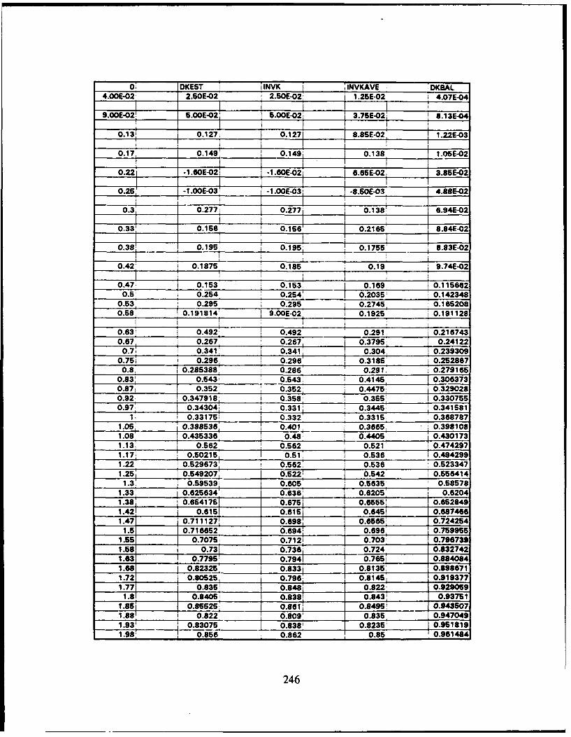
o0 DKEST I INVKKAVE_________ ____I___ INVKAV I MAL4.OOE-02 2.50E-02' 2.50E-02' 1.25E-02 I 4.07E-04

9.042 __{: 5.00E-02 2 3.75E-02! S.13E44

0.131 1___ 0.1271027 8.85ET-02 1 1.2.2E-030.1T0.149W 1 -02

0.17 __ .14 __ 0.149 0.138 1.05E-02

0.22 -1.60E-02 -8.E-065E02 3.85E-020.26 -I .OOE-03 E0

- 10E-030 -8.60E-03 4.88E-02

0.3 0.20277 0. 138' 6.94E-02

0.33 0.156 i05 0.2165 8.84E-02

0.380- 0.195 0.1951 0.1755 8.83E-02

0.42 0.1875 0.185 0.19 9.74E'020.47 0.1015z53 0.153 0.169 0.115662

0.5 0.254. 0.254' 0.2035 0.1423480.53 0.295 j 0.295 0.2745, 0.1652080.58 0.191814 [ 9.OOE-02, j 0.1925 0.191128

0.63 0.492! 0.492 0.291 0.216743

0.70.267 0.267, i0.3795, 0.241220.7 0.341' 0.341 0.304, 0.239309

0.75; 0.296 0.296' 0.3185' 0.2528670.8, 0.285388.' 0.286' 0.291, "0.279165

0.83: t 0.543, 0.543, 0.4145 0.3063730.87: 0.352 0.352; 0.4475 0.3290280.92_ 0.347918_ i 0.358_ 0.355: I 0.3307550.92 0.343041 0.3315 , 0.3445! 0.3415810.97: 1 34 04 0.331751 _________

1. 0.33175 1 0.332 0.3315 , 0.3687871.05, 0.3885386 i 0401 0.3665. 0.3981081.08 0.4353360.48 0.4405 0.4301731.13! 0.562 0.562 0.521 0.4742971.171 0.50215 I 0.51: 0.536 10.4842991.22 0.529673, 0.562' 0.536 0.5233471.25, 0.5492071 0.522! 0.542 I 0.556414

1.3_ 0.59539: 0.605 0.5635i ' 0.585781.33, 0.625634 0.636, 0.6205' 0.62041.38 0.6541 75 0.675 0.066555 0.6528491.421 0.615 0.61- 0.64S 0.6874661.47 0.711127 0.698, 0.6565 0.724254

1.5 0.716652' 0.694ý 0.696' 0.759955

1.55 0.7075; 0.712 i 0.703! 0.7967391.58' 0.73_ 0.738 0.724 0.8327421.63 0.7795 0.794 0.765 i 0.8840841.68 0.82325 _ 0.833 i 0.8135: 0.8986711.72 0. 0525 0.788 0.8145 0.9193771.77 0.835 0.848 0.822 0.929069

1.9 0.S40* 0.831 0.8431 0.937511.85_0.8552__ 0.861V 0.8485! 0.9435071.88 0.822 0.909' 0.835, 0.947049

1.93' i .30.83188 0.8235 0911

1.98, 0.856 0.862 , 0.85 098148,

246

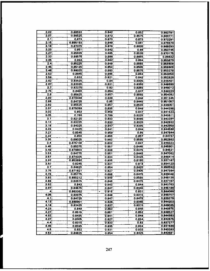
2.02 0.88593 0.842 0.852 0.9637912.07, 0.86525. 0.873 1 0.8575 0.969771

2.1 0.873 0.873, 0.873 0.9732912.151 0.895193' __0.849 ___ 0.861 0.9755792.181 0.87075! - 0.878' 0.86351 0.97579

2. 3 0..863F.42t 0.969293

2.23 0.851 0.842: 0.86 0.9507462.271 0.86925.! 0.865, 0.85351 0.9701762.32i 0.86575 0.866: 0.8655, 0.966322.351 0.863ý 0.862! 0.864, 0.9538792.4 0.85225 0.849 0.8555 0.959808

2.48 0.85125 0.852 0.8505' 0.9596092.45 0.880251___ 1 0.863; 0.T575; 0.9532782.53! 0.8645, 0.865; 0.864 0.9530592.58 0.832 0.821; 0.843 0.9528262.62! 0.835251 0.84 0.83051 0.9464812.67 0.833251 0.8310. 0.8355: 948699

2.7, 0.822751 0.82! 0.8255_ 0.9460122.75; 0.8455, 0.8541 0.837 0.948223

2.8 0.85625 0.857 1 0.8555 0.9540822.83; 0.879449. 0.8391 0.848 0.9513452.88; 1 0.84725 0.85I 0.8445' 0.9510572.921 i 0.855251 0.857 0.8535' 0.9360512.97 0.875099 0.835. 0.846' 0.9442983.02 0.853 0.859 0.847, 0.9415233.05 0.786 0.786 0.8225 0.943611

3.1' 0.82125 0.833 0.8095, 0.9432883.13 1 0.83225. 0.832: 0.8325 0.9429323.18 0.84325, 0.8471 0.8395: 0.9425583.23 08425' r 0.841; 0.844, 0.9445983.27'i 0.85451 i i

3.27, 085450.859' 0.85 , 0.9478443.32 _ 0.856 0.855 0.857 0.947373.35 0.86025 0.862; 0.8585, 0.952992

3.4 0.875108 0.832 0.847 0.9463233.45 0.85075 0.857 0.8445, 0.9458013.48 0.876903 1 0.838 0.8475: 0.945213.53 0.847751 0.851 0.8445 : 0.947062

- 3.57 0874305 . 0.834 _ 0.8425, 9464143.57 .J 0.84 ____0.946__14

3.62 ' 0.853896: 0.805 t, 0.81951 0.9371873.67 0.8245 0.831 i 0.818 - 0.934123

3.7 j 0.84825 i 0.854 0.8425' 0.9505923.75 0.871621 0.827 0.8405 0.9473643.78 0.85775 0.868 0.8475, 0.9490483.83 0.885212 0.849, 0.8585, 0.9481363.88 0.84675 r 0.846 0.8475 0.9471973.92 0.843 . 0.842' 0.844i 0.943763

3.97 0.84570184.75 ,.. 0.847; 0.84451 0.9451860.8633624 0.815, 0.831 0.944086

S0.83975 0.848, 0.8315. 0.9467074.1 0.84725 0.8471 0.84751 0.939379

0.868901 0.92 0.8385 0.9442034.18 0.83425 0 .8 3 7

' 0.8315: 0.9480354.23, 0.849 0.853 0.846; 0.9439754.27 0.8515; 0.851' 0.852' 0.948527"4.32i 0.8435 0.841 0.846 0.9443934.37 i 0.8305 - 0.827 0.834: 0.942676

4.4 0.8315' 0.833! 0.83 0.9372774.45 0.8345 0.835' 0.8341 0.941566

4.5 0.832 0.831 0.833 10.9432834.53 0.84825 0.854 0.8425, 0.943681

247

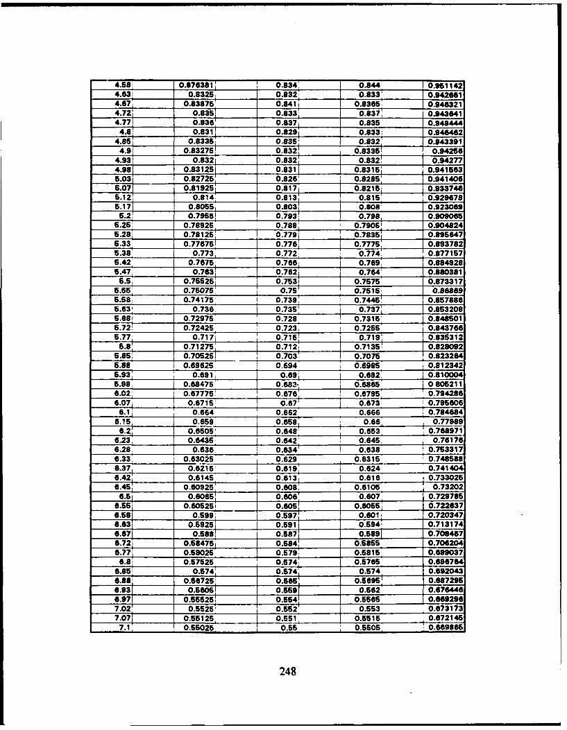
4.58: 0.876381 0.834ý 0.844, 0.9611424.63i 0.83265 0.832 0.833' J 0.9426614.67, 0.83875' 0.841t' 0.8365: 0.9463214.72, 0.8351 0.833; 0.837: 0.9436414.771 0.836, 0.8371 0.835 * 0.949444

4.8! 0.831 0.829__ 0.88331 0.9484624.85 0.8336 0.835' 0.832 0.943391

4.91 0.83275! 0.832! 0.8335! 0.942564.931 0.832i 0.832' 0.832! 0.942774.981 0.83125 0.831 0.83151 0.9415635.031 0.82725 0.8261 0.8285' 0.9414065.071 0.81925; 0.817 0 .8 2 15 ; 0.9337465.12! 0.814, 0.813, 0.815' 0.9296785.171 0.8055 I 0.803 0.808' 0.9230695.2, 0.79551 0.7931 0.798, 0.909065

5.25 0.78925. 0.788 0.7906! 0.9048245.28! 0.78125 0.779 0.78351 0.895647

5.33 0.776765 1 0.776; 0.7775 0.8937825.38' 0.773, ± 0.772. 0.774. 0.8771575.42 0.7675 j 0.766; 0.769, 0.8849285.47 0.763 0.762 0.764; 0.880381

5.5, 0.75525, ' 0.753 0.7575; 0.873317.55 t0.75075.' 0.75 ! 0.7515' 0.86869

5.58 0.741751 I 0.739W 0.7445! 0.8578865.63' 0.736 1 0.735' 0.7371 0.8532085.68; 0.72975 0.728 0.7315 0.8485015.72: 0.72425 0.723. 0.7255'. 0.843766

5.77 0.7171 - 0.7156 0.7191 0.8353125.8 0.71275' 0.712: 0.7135! 0.828092

6.85: 0. 0.703' , 0.7075 0.8232645.98 i 0.69625 i 0.694 _ 0.6985 , 0.8123426.93__ 0._91_ 0.9:°'9 0.692__ _ 0.8100045.98 . 0.88475' 0.683- 0.6865 0 805211

6.02: 0.677756 0.676: 0.6795' ' 0.7942866.07______ 0.6715SW6.07i 4 _0.6715: 0.67 0.6731 10.795606

6.1: 0.664 0.662 0.666 1 0.7848846.15, 0.659 7 0.658, 0.66 0.77989

6.2: 0.6505, 0.648 0.653 0.7689716.23, 0.6435, 4 0.642: 0.645. 0.761766.28 0.636, * 0.634' 0.638 0.7533176.33, 0.63025 0.629 0.6315 10.7485886.37, 0.6215: 0.619,: 0.624' 0.7414046.42 0.6145 0.613: 0.616 0.7330256.45 0.60925' j 0.608. 0.6105, 0.73202

6.5 0.60650. 0.606' 0.607 0.7297856.55 0.60525' 0.606' 0.6051 0.7226376.58 0.599; 0.597, 0.601! 0.7203476.63 0.5925 ' 0.591 0.594; 0.7131746.67 0.588; 0.587 0.5891 0.708476.72 0.584751 0.584 0.5855, 0.7062046.77 0.58026 0.579: 0.5815: 0.699037

6.8 0.57525 0.574, 0.5765: 0.6967646.85 0.574' 0.574 0.5741 0.6920436.88 0.66725 0"5665t 0.56965 0.6872956.93 0.5605' 0.559 0.662 0.6764466.97 0.55525. 0.554 0.5565 0.6692987.02 0.5525' 0.552' 0.553 0.6731737.07 0.65125L 0.551. 0.515 } 0.672146

7.1 T 0.55025 0.55 0.5505 , 0.669865

248

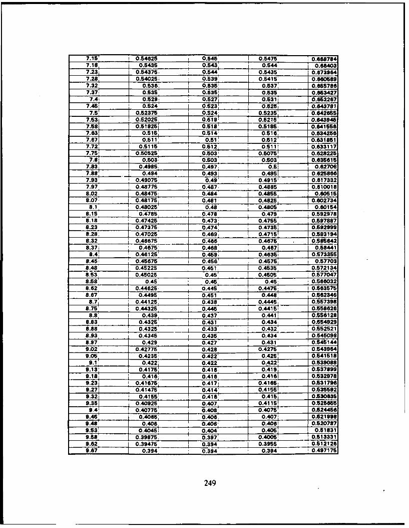
7.15' 0.54625 0.5457 1 0.5475 _0.6687847.18, io.5,5 0 .5431 ."OW7.18, __________________________0.54375, 0.53 0.544 0.66403

; 0.54375 0.544 0.5435, 0.6739647.28, 0.54025, 0.539: 0.5415 0.6605897.32: 0.536! 0.535: 0.537: 0.6557867.37j 0.535 0.35!5 0.5351 0.653427

7.4A 0.529! 0.527 0.5311 0.6622677.46 ' 0.524: 0.523 0.525I 0.643781

7.5 0.52375: 0.524 0.5235 0.6426557.53 0.52025 0. 19:i 0.643946

7.581 0.51825; .0.5181 0.5185 0.6415567.63 0.515 0.514' 0.516' 0.6342567.67' 0.511 0.51 ! 0.512' 0.6318517.72' 0.5115 0512 0.511 1 0.6331177.75; 0.50525' 0.503_ 0.50751 0.628225

7.8 0.503 ! 0.503: 0.503 0.6356157.83 0.4985' 0.497: 0.5: 0.627067.88 0.494' 0.493; 0.4951 0.6258667.93: 0.49075 0.49' 0.4915 0.6173327.97 0.48775 0.487 0.4885 0.6100188.02, 0.48475: 0.484, 0.4855, 0.605158.07 048175 0.481 0.4825 0.602734

8.1 0.481 0.4805o"0 o.01548.15 0.4785 I 0.478 0.479. 0.5929788.182 0.47425 0.473 0.4755, ' 0.5978878.23_ 0.47375 0.474, 0.4735 0.5929998.28 0.47025 0.469. 0.4715 0.5831948.32' 0.46675 0.466 0.4675. 0.5856428.37 0.4675 0.468 1 0 .4 67 1 0.5 844 1

8.4 0.46125' 0.469 0.4635 i 0.5733558.45; 0.45675 0.456' 0.4575' 0.577038.48' 045225 0.451 1 0.4535 ' 0.5721348.53t 0145025 0.45' 0.4505 0.5770478.58 0.45 0.45 0.45 0.560328.62 0.44625 0.445 0."75' 1 0.5663758.67 0.4495 0.451; 0.448!_! 0.562346

8.75 0.44125. 0.438' 0.4445 0.5573988.75_ 0.44325 0.44C5 0.4415 j 0.558626

8.8, 0.439, i 0.437, 0.441 1 0.5561288.83 0.4325 0.431; 0.434. 0.5549298.88, 0.4325 0.433 0.432 0.5525218.93 0.4345 0.435 , 0.434 0.5450988.97 0.429 0.427 0.431 0.545144

9.021 0.42775 0.428 0.4275 ,0.5439649.05 _ 0.4235 0.422! 0.425! 0.541518

9.1 0.422; 0.4221 0.422' 0.5390889.13 0.4175 0.416 0.419 0.537899

.180.41 0.4168 0.416 0.5329789.23 0.41675; 0.417 0.4165, 0.5317969.27 0.41475 0.414 0.4155! 0.5355929.32 0.4155 + 0.416: 0.415 0.5306359.351 0.40925 0.407 0.4115! 0.525655

9.4 0.40775' 0.408' 0.4075! 0.5244569.45 0.4065; 0.406! L 0.407' 0.5219989.48 0.406, 0.406 0.406 0.5207879.53 0.4048; 0.404ý 0.405! 0.518319.58 0.39875 0.397 0.4005 0.5133319.62 0.39475 0.394i 1 0.3955 ,0.5121269.67i 0.394 0.394 0.394 !0.497175

249

9.7 0.394 T 0.394; 0.394' 0.5072159.75 0.391: 0.39' 0.392- 0.508499.78, 0.38475, 0.383 0.3865 1 0.507279.831 0.3875: 0.3898 0.386 0.5023369.88 0.389751 0.39' 0.38956 0.497369.921 0.3885 0.388 J 0.389 0.5011139.971 0.3895 0.39 0.389 0.502364

10 0.38851 0.388! 0.389 0.50109310.05 0.385 0.384' 0.386 0.49857110.1 0.3871 0.388, 0. 0.073110.13_ 0.3827 _ 0.3811 8.3845ý 0.494764

10.1 o 0.375 0.3791 0.386 0.48.731

10.23 0.378, 0.375! 0.377: 0.48846310.27 0.37275' 0.372, 0.3735' 0.48345110.32 0.369751 0.369' 0.37057 0.47469410.35 0.369. 0.369 0.3698 0.482192

10.4 0.363 1 0.361! 0.365: 0.48343210.415! 0.364! 0.365: 0.363: 0.48470310.48: 0.36575 0.366' 0.3655 0.47594710.53 0.38375 0.363. 0.3645 10.47717610.57 0.3615' 0.361' 0.362; 0.4759110.62,; 0.3565 0.355 - 0.358 0.47089310.67! 0.355: 0.355' 0.355 0.472151

10.7 _ 0.358 0.359 0.357' 0.46965110.75 0.35675 0.356' 0.3575' 0.470874

10.8 : 0.3545' 0.354 0.365' 0.45960310.83. 0.354 l 0.354! 0.354 0.4645810.88 1 0.3525 0.352' 0.3531 0.46580110.92: 0.35125' 0.3511 1 0.3515, 0.4832710.97, 0.34575, 0.344, 0.3475 0.46823811.02 0.34625' 0.347 0.3455; 0.45948111.05: 0.34775 0.348, 0.3475' 0.44670411.1 0.34575 0.3458 0.3465 0.458164

11.15_ 0.34425' 0.344' 0.3445, 0.46938

11.18 0.34325__ 0.343 0.3435 0.46434511.23 0.34375' 0.344 0.3435 1 0.46305311.27, 0.341 0.34 0.342;' 045425511.32i 0.3385 0.338' 0.339 0.44648211.371 0.338, 0.338 0.338 1 0.450425

11.4 : 0.3365 0.336 0.337; 0.44788211.45 0.33525 5 0.335 1 0.3355 0.44658811.5_ _ 0.34025, 0.342 0.3385- 0.444045

11.53 0.33675 ' 0.335 0.3385, 0.43896311.58 0.332 0.331! 0.333 0.44015____0.305333________ 0.44015___ ____

11.62 0.33025' 0.33 0.3305 0.44135611.67! 0.330754 0.331: 0.33056 0.43006211.72 0.334 0.335 0.333: 0.44000611.75 0.329; 0.327 0.331 0.423674

11.8 0.33075 0.332' 0.32951 0.42986811.851 0.326 0.324 0.328 . 0.43478811.88. 0.3255, 0.326: 0.3251 0.42973811.93 0.32225; 0.321 0.3235, 0.43717711.97 0.32025, 0.32' 0.3205' 0.43212812.02 0.32375' 0.3251 0.3225: 0.4270812.07 0.32125; 0.32 0.32251 0.427007

12.1 0.3171 0.316: 0.318: 0.42194812.15 _0.3145 0.314 0.315, 0.42320712.18 1 0.31475 0.315 0.3145' 0.422082

1 2 .2 3 1 0.30975 , 0.308 0.3115 0.419648

250

12.28' 0.314: 0.316' 0.312 0.42116212.321 0.313' 0.312 0.314' 0.42001112.37 0.31125: 0.311j 0.3115 0.41496312.42 0.3096 0.309 0.31 0.416412.45 0.308 0.305 0.307' 0.417925

12.51 0.30425' 0.304 0.30451 0.41289712.55 0.300251 0.299$ 0.3015 0.41439512.58 0.30275 0.304: 0.30156 0.41199812.63 0.30175! 0.3011 0.3025, 0.41610312.87 0.2995 0.299 0.3! 0.40847112.72 0.301255 0.302' 0.3005 0.41650512.771 0.30125 0.301 0.3015 0.404"47

12.81 0.2995' 0.299 0.3 0.40905212.85 0.2975, 0.297 0.298 0.40402312.88 0.29625! 0.296C 0.2965' 0.40552612.93, 0.29525: 0.295' 0.2965 0.40442112.98 0.29651 0.297; 0.296' 0.40592713.02 0.29825. 0.296 0.2965 1 0.40742313.07! 0.29525 0.295: 0.29551 0.40500613.12 0.29425 0.294 0.29461 0.40389613.151 0.29175, 0.291' 0.29251 0.40148313.2! 0.291: 0.291 4 0.291: 0.402992

13.25 0.29325 0.294, 0.2925 0.40068913.28; 0.2895 0.288. 0.2911 0.40208413.331 0.28876 0.289 0.2885 0.4009913.37, 0.286 0.285, 0 287 0.39858713.427 0.27825 0.276! 0 .2 8 051 0.40011313.47 0.2835: 0.286 1 0.2811 0.392542

13.5: 0.28675' 0.2871; 0.28651 0.39667713.55 0.28475. 0.284, 0.2855 0.40210613.58' 0.28325 0.283 0.2835- 0.39971513.63: 0.2815 0.281; 0.282ý 0.39471613.68 0.278 0.277, 0.279' 0.3962513.72 0.2815 0.283, 0.28' 0.391274

13.77: 0.2815 0.281 0.282, 0.39280113.82 0.28175' 0.282 0.28151 0.39433213.85' 0.27825' 0.277, 0.2795 0.389334

13.9g 0.27625 0.2768! 0.2765, 0.38436113.93: 0.276, 0.276: 0.276' 0.38851213.98: 0.27525, 0.275 0.2755r 0.38092414.03, 0.27575 0.276 0.2755 0.38914.07j 0.27525: 0.275 0.2755 0.38663314.12: 0.27125 0.27' 0.2725, 0.38557414.17 1 0.2685 _: 0.2688 0.269 0.38323

14.2! 0.2711 0.272' 0.27 0.38481114.25 0.2705 0.27.: 0.2711 0.382462

14.3 0.2715 _0.272, 0.271! 0.38794714.33 0.275751 0.277' 0.2745 0.38298314.38 0.26875 0.266, 0.2715 0.38060914.42 0.26525! 0.265' 0.2665 0.3756714.47 0.285' 0.265: 0.265 0.36812414.52 0.2665 0.287; 0.266 0.37624214.551 0.264 0.263 0.265 0.377827

14.6 0.26 0.259, 0.261 z 0.37290214.65 0.261261 0.262, 0.26051 0.36799214.68 0.26125i 0.2615 0.37220914.73 0.258: 0.257 0.259, 0.3738214.77 0.26 0.281; 0.259 0.37153214.82, , 0.26175_ 0.262' 0.2615, #0.373145

251

14.87 __0.26125 0.261i 0.2616! 0.3721414.9 0.26875 0.258s 0.2595 0.376312

14.96 0.261'i 0.262! 0.26: 0.37141215 0.259 0.258 0.26 0.370385

15.03 0.255: 0.254 0.256. 0.36548815.08 0.2656! 0.266 0.255; 0.36708116.12 0.2675 0.258 0.257' 0.36478815.17 0.2535_ 0.252 0.2551 0.359899

15.22 0.252; 0.252 0.252; 0.36539

15.275 0.2456126! .24

15.5 0.241 0.2411 0.2515 0.36570615.3 0.253256 0.254: 0.25251 0.360847

15.357 0.251751 0.2514 0.2525' 0.36246515.38 0.2525! 0.253 0.252 0.36104715.43 0.24925' 0.245 0.2505 0.35921215.471 0.242 - 0.244 0.246! 0.35826315.92, 0.2412 0.24: 0.242! 0.36990615.571 0.246751 0.2491 0.2443 0.357693

15.6 0.24753 0.247 0.243 0.35933615.65 0.24925, 0.254 0.24"5 0.360983

15.7. b0.24775 0.247 ' 0.24"5 0.38003515.731 0.2395 0.237, 0.242 0.3570115.78l 0.243' 0.245 0.2413 0.35301716.83 0.2435 0.2453 0.245 0.35727515.87! 0.242 0.2413 0.2433 0.35635215.92, 0.2385 0.243. 0.2423 0.350861156.973 0.2435 0.2437 0.2435 0.34936

16 0.243 0.243 0.243 0.35104216.05, 0.23825, 0.238, 0.2425! 0.350141

15.18 0.24125; 0.241 i1 0.2415 0.35183416.13 0.23955 0.239 0.249 0.34164916.18! 0.2375 0.237, 0.238 1 0.34276916.722 0.23325 0.232' 0.2345', 0.3504916.7 0.23425' 0.235, 0.2335' 0.33349

16.75I I 0.2 3875t % 0.2429 0.23751 0.35008816.8' 0.23775 0.2372 t 0.2385 0.34792416.4'02 0.2385 0.2331 0.28:1 0.347067

16.458 0.23825i 0.238, 0.2385' 0.3513916.93i 0.2365: 0 .2345 1 0.236 0.33406416.539 0.23025. 0.2293 1 0.2315 0.33934516.58, _ 0"2305 0.2293 0.2293 0.34112316.62 0.22975 023 20.2295 0.34290818.7, _ 0.235 0 .232 0.231, 0.33821817.15 0.232' 0.232 0.232' 0.3348175 0.22975: 0.229 0.2305 0.32497716.82 0.22925 0.229 0.229 0.33949616.861 0.232Z 0.233; 0.2311 0.3415

16.388 0.23075! 0.23' 0.2315! 0.33940916.931 0.22625' 0.22r, 0.2275, 0.33473916.971 0.228751 0.23 0.2275 i 0.336567

17.023 0.23075 0.231 0.2305 0.33579517.071 0.228754 0.228, , 0.2294: 0.340204

17.14 0.228 0.228 0.228 0.3321617.151 0.2265, 0.226 0.2270.17.21 0.229 0.23' 0.228ý' 0.3327717.23l 0.2292S! 0.229; 0.2295' 0.334611

17.*28 0.22825, 0.228 .23 0.33365717.33! 0.225, 0.224! 0.226' 0.33572117.371 0.224ý 0.224,; 0.224 i0.331116

17.421 0.224 , 0.224, , 0.224,, 0.329109

252

17.47i 0.224, 0.224 ;7 0.224 i 0.33099317.65 0.22025: _0.219 0.2215' S0.328994

17.55 0.2205 0.221' 0.22 0.32831317.68 0.22025 0.22' 0.2205: 0.330223

17.63' 0.22075. 0.221 0.2205, 0.328256

1 0.22025 022 0.22056 0.323717.72 0.21775! 0.2171 0.2185' 0.31915117.77 0.217' 0.217i 0.2171 0.31850417.82 0.21775; 0.218' 0.2175, 0.32304517.85 0.215 0.214T 0.2108 0.316933

17.9! 0.21475: 1 0.2151 0.2145; 0.32049417.95, 0.21575 ;. 0 .2 1 6 0.21551 0.31987717.98 0.20925 . 0.207 0.2115' 0.3179661803 0.21375 i 0.216' 0.2115, 0.313518.081 0.213 0.2121 0.214. 0.32196518,12_ 0.21125 0.211_0.2111 0.31361118.17! 0.211 -0.2111 0.211V 0.31303618.221 0.21325 0.214, 0.2125 0 30858418.25, 0.211 0.21 0.212 0.317077

18.3. 0.21 0.21 i 0.21i 0.31263918.35; 0.2131 0.2141 i 0.212 0.31079918.38 0.214 0.214: , 0.214' 0.299886

18.43: 0.2125, 0.212' 0.213; 0.31228418.47 0.212i 0.212 0.30786118.52i0.2112:• 0.212,

18.52 0.21125, 0.2111 0.2115, 0.30992118.57 0.20950.209 0.211 0.299038

18.6 0.2075 0.207, ' 0.208 0.31018318.65 0.21075 I 0.2121 0.2095 . 0.309687

18.71 0.212.22 ' 0.212 0.29493718.73. 0.21425; 1 0.215 0.2135 J 0.306091

18.78 1 0.2135 - 0.213 0.214. 0.30558618.83 0.21075 0.21 , 0.2115: 0.303818.87 0.21 ' 0.21' " 0.21! 0.359218.92 0.21075 0.211- 0.2105 i0.30155718.97, 0.21175 0.212 0.2115 0.301091

19 0.2075 , 0.206 ' 0.209 T 0.299331

19.06' 0.20525, 0.205' 0.2055 0.29500619.08 0.2035, _._0.203, L 0.204 0.29069519.13_ 0.2015 0.201, 0.202 0.292872

19.18 0.20325 0.204 0.2025. i 0.29247219.221 0.20325 0.203' =0.2035 0.29077619.27, 0.2015 __0"201 __ 0.202, 0.29297219.32 0.20475 0.206 0.20351 0.288707

19.35: 0.203, o0202 0.204, 0.2883219.4, 0.20275 " 0.203, 0.2025! 0.286857

19.46 0.2015 0.201_ 0.202: 0.296357

19.48 0.2201 0.201 0.201, 0.28464619.53 0.20175. 0.202' 0.2015. 0.283008

19.58 _ 0.2005! 0.2 0.201 0.28266919.62 0.19925 0.1991 0.19951 0.281048

19.67 0.199 0.199w 0.199 0.2807319.72' 0.20125, 1 0.2021 0.2005' 0.28301219.75! 0.199 0.198' 0.21 0.281407

19.8! 0.20025 0.201! 0. 1995: 0.277231

1983 0.2025 0.203! 0.202 0.27952819.88 0.203! 0.203 0.203! 0.275348

19.93, 0.2045 , 0.205F 0.204, 0.27765319.97 0.2035 I 0.203, 0.204. 0.27736520.02 0.2015, 0.201 * 0.202 0.273207

253

20.07 0.20025' 0.2. 0.2005' 0.26906220.11 0.197 1 0.196. 0.198 0.267517

20.15 0.199, 0.2 0.1981 0.26987620.2 0.197 0196 0.198 0.268349

20.23 0.19675 0.197, 01965' 0.2645120.28, 0.19925 0.2 0.195: 0.26"3120.33 0.1932_ 0.191 0.1955 0.26253620.37 0.19325' 0 194o 0.2823612o0.42 0. 194; o.194_ 0.194, 0.26089320.47 0.1912 0.191 0.192, 0.2636120.5 0.194 0.19! 0.194 0.256688

20.55' 0.19225 0.193, 0.1915. 0.25525320.58 0.19525I 0.196! 0.1945' 0.25511320.631 0.19525; 0.195' 0.1955 0.25367620.68! 0.19575. 0.196, 0.1955' 0.25354420,72! 0.2005' 0.202 0.199. 0.2495320.77 0.181: 0.181 0.1915i 0.24809620.821 0.1795' 0.1791 0.18i 0.24414320.85 0.178251 0.178, 0.1785 0.237618

20.9 0.18175. 0.183 0.1805, 0.23628920.93! 0.18075: 0.18' 0.1815 0.236248

2 0 .98 ; 0.189. 0.18 0.18i 0.24140221.03 0.1845 0.1868 0.183 1 0.23749921.07T 0.18075 0.179 0.1825 0.23358621.121 0.182 0.183: 0.181 0.24912821.17 0.17775 0.176 0. 1795' 0.228409

21.2_ 0.176 0.176' 0.176. 0.23491421.25 0.17225, 0.171: 0.1735 0.23106821.28 0.17775 0.18' 0.1755! 0.22724821.33! 0.1815! 0.1821 0.181 0.22600121.38' 0. 18275 0.183 1 0.18251 0.23252421.42 0.18 0.179 0.181, 0.23120521.47: 0.17675 0.17k, 0.1775' 022099121.52, 0.176 0.176 0.176W 0.22969721.55, 0.1745 0.174' 0.175. 1 0.22591321.6 0.1785 0.18 0.177 0.222143

21.65, 0.177, 0.176 0.178. 0.21836221.688 0.1775i 0.178 0.177' 0.22436121.73' 1 0.1765' 0.176' 0.177 0.22060521.783 0.18275 0.185 0.1805 0.221743

21.82 0.182 0.181 i 0.183 0.22163921.87 0.18325; 0.184 0.1825 0.220336

21.9 0.1795 0.178 0.181 0.21659321.95' 0.1795' 0.18! 0.179_ 0.216533

221 0.18! 0.18' 0.18: 0.2189222.03 0.17925' 0. 179! 0. 1795; 0.21765522.08, 0.179751 0.181 0.17951 0.2139622.13, 0.17851 0.1781 0.179, 0.2139322.171 0.17575' 0.175' 0.1765! 0.21025422.22 0.17875 0 O. 18! 0.1775, 0.20903922.25 0.17625 0.175, 0.1775 0.20M037

22.31 0.1765: 0_. .177 0.176' 0.206396202.35 ' 0.17925 0.18 0.1785' 0.207859

22.381 0.1771 0.176' 0.178: 0.20666222.431 0.176! 0.176: 0.176t 0.20304522.481 0.181533 0.169! 0.17256 0.20309922.52; 0.172. 0.173 i 0.171_ _ _ 0.19952122.57 0.17, 0.169 0.171. 0.20082322.62; 0.17125 0.172 0.1705 0.200925

254

22.65 0.17425: 0.175 0.1735' 0.19S8e222.7 1 0. 17425' 0.1741 0.1746! 0.196249

22.75 1 0.17175 0.171i 0.1725' 0.19638122.78: 0.17025 0.17 0.1705 0.19283322.83: 0.17525 0.177 0.17351 0.19175322.87, 0.178962 0.171 0.174 0.19188622.92 0.1725 0.173 0.172. 0.19082122.97 0.16775: 0.166 01695, 0.190981

231 0.16825 0.169 0.16751 0.18751223.06, 0.16975' 0.17! 0.1695' 0.190142

23.1 0. 17;" 0.171 0.17i 0.18667823.13 0.16325 0.161 0.1655 0.18932423.18 0.167751 0.17 0.16655 0.185904

23.22 0. 173469 0. 167 0.1685W 0.18490823.27' 000.1671 0167 0.18758823.32_ 0.173: 0.175: 0.171' 0.18417823.35 0.168251 0.166 0.17065 0.184412

23.41 0.1684411 0.165' 0.1665 0.16882223.46' 0j16575, 0.166' o. 0.16651 0.18252623.48; 0.165539 0.162 0. 164 0.17061623.53 0.1635 0. 164 0.163 0.17946423.58' 0.16475 0.165 0.1646 0.19441923.621 0. 1665' 0. 167 ' 0.160 178877

23.67 J0.167847 0.163 0.165 0 17S54123.7 0.165888 0.161 0.162 1.174665

23.75' 0.164 0.165 0.163i 0. 17746323.8' 0.167274i 0.161! 0.163. 0.177822

23.831 0.16175 0.162' 0.1615i 0.1746423.88! .1635 0.164 0.163 10.;17370323.93 0.165364 0.16 0. 162' 0.17409123.97, 0.16225 1 0.163 0.1615 0.17327924.02' 0.166562, 0.163' 0.163 0. 17368624.07, 0.166515 0.161: 0.162: 0.176645

24.1: 0.16325 0.164 0.1625: O.'7575724.15 0.16475 0.165 0.1645 0.17862924.18 0.166249 i 0.163 0.164 0.17174724.23 0.163 0.163 0.163, 0.1868424.28 0.16525, 0.166 0.16465 0.17510224.32 0.16 0.158 0.162 0.16824424.37; 0.161, 0.162 0.16 1 0.17483624.42 0.165223 : 0.162 0.162 O.f17166824.45 0184483 0.161 _ 0.1615 0.17095

24.5 j0.162267 0.159 0.16 0.16780224.55, 0.1605 0.161 0.16 0.17076824.58 0.162433. 0.157 0.159 0.17129924.63 0.1585i 0.159, 0.158! 0.1681924.68 0.15075: 0.1481 0.15351 0.167S2724.72 0.154' 0.156; 0.1521 0.16812324.77 0.157516', 0.153' 0.1545 0.165048

24.8 0.156. 0.157; 0.155i 0.16808824.85 0.1601768 0.1581, 0.1575; 0.166029

24.9 0.1565 0.156! 0.157i 0.17661424.93 0.15675 0.157! 0.1565i 0.168914

S24.98, 0.159479' 0.157: 0.157' 0.1644382S.03 0.160504: 0.157i 0.157 0.16751325.07 0.6313 0. 1671 0.162 0.16693825.12 0.161 0.1591 0.163: 0.17000325.17 0.158852, 0.1551 0.157, 0.164657

25.2: 0.156504 0.152 0.1535 0.1640I1

255

25.251 0.158515: 0.15Mi 0.155; 0.15i04625.28 0.1541568 0.154, 0,15656 0.15196925.33! 0.154904! 0.151 0.1525' 0.16121121.38 0.15475 0,156! 0.1535: 0.16437525.42 0.15145 0.15 0 . 1 5 3 ! 0.16143326.47 0.14, 0*.156 0.153! 0.164696

25.6 0.1583911 0.1671 0.1565! 0.16167325.55 0.1575851 0.153 1 0.155 0.164755

25.6 0.154852 0.148 0.1505i 0.16645725.63 0.1481 0.1 0.1481 0.16498425.68 0.154 0.156 0.152 0.16461925.73 0.15908! 0. 156 0.156 __ 0.1652425.77; 0.151824 0.153! 0.1545' 0.14797125.82! 0.1569721 0.155 0.154 0.16191625.87' 0.1573568 0.155 0.1541 0.16506725.9 0.15375 0.154 0.16 0.166832

25.95 0.146 0.146 0.15 0.165401

261 0.15125: 0.1531 0.1495 0.16820526.03 0.155766. 0.15i 0.1515 0.16579926.08 0.153 0.154 0.152. 0.16660826.13 0.159272 0.158. 0.156i 0.16381626.17 0.1535 0.152 " 0.155 0.16701926.22' 0.15575 0.157i 0.15465 0.17024626.25: ' 0.15325. 0.152: 0.1545, 0.163868

26.3 0.152 0.152- 0.152' 0.16471526.35 0.1275 1 0.153 0. 1525 0.16677226.38 0.156878 0.151 152 0.16763326.431 0.154636 °1491 0.152015 0.16490826.48: 0.153199 0.1471 0.1481 0.16459826.52, 0.1485 0. 149 0.148; 0.16550226.57:, 0.14975 0.15 0.1495' 0.165211

26.621 0.15375 0.155: 0.1525i 0.16612426.65' 0.156611 0.151i 0.153' 0166833

26.7 0.14575 0.144 0.1475M 0.16676126.731 0.147 0.148 0.146ý 0.15811726.78! 0.1465 0.146' 0.147i 0.16987426.83 _ 0.1535 0.1561 0.151 0.16484426.871 0.157565 0.151! 0.1535' 0.16819526.92! 0.151 0.151 0.151: 0.165566526.97 0.1532811 .. 1 0,1454 0.166344

27._i 0.14825 0.149, 0.1475 0.1627482 0.1507171 0.145! 0.14 0.160152

27.1, 0.1465 0.147, 0.146 0.16117427.131 0.1455. 0.145: 0.146ý 0.16727.18 0.145 0.1461 0.1465 0.16084127.22 0.148431 0.143' 0.144 0.15829227.27 0.1445 1 0.1451 .144 0.155675627.32 0. 148741 0.1431 0.144 0.16922427.35 0. 14675! O.14 8 1 0.1455' 0.162708

27.4 0.14875 0.149 0.1485 0.16378527.45 0.1437 0.141 0.145i 0.16126727.48 0.14175 0.142 0.1415 0.16117827.53 0.142 0.142 0. 142!, 0.16229727.68 0.14875' 0.151 0.14ff 0.15622627.62 0.136 0.136' 0.14351 0.15973527.67 0.1368 0.138 0.136 0.157292

27.7 0.136, 0.136 0.136 0.15246327.75 0.1345 0.134 0.1351 0.156043

27.8. 0.1325 0.132' 0.133 0.153636

256

27.856 0.135. 0.136: 0.134 0.15724327.88! 0.133, 0.132i 0.134. 0.1608527.93: 0.132 0.132i 0132L 0.15847527.97 0.1335': 0. 134 0. 133! 0.1621128.02! 0.13025: 0.129 0.13153 0.16214828.07 0.134256 0.136' 0.1326- 0.15981

28.11 0.13675 0.137 0.1365 0.16686128.15' 0.13925 0.14 0.1385, 0.163516

28.2' 0.1445: 0 . 1 4 6 : 0. 143' 0.16117128.23 0.133. 0.133' 0.1395 0.162416

2 8 .2 8 0.13375! 0.134, 0.1335' 0.16250328.32! 0.130265 00129 O.1315 0.16379828.37! 0.13425 j 0.138 0.13251 0.18191628.42; 0.1345' 0.134 0.135 0.16762528.45 0.1325, 0.132 0.133; 0.168947

28.6 0.13875 0.141 0.1365! 0.168908228.55 0. 13875 0.1381 0.13951 0.17280328.58 0.13275 0.131 0.1345i 0.17053628.63 0.1355 0.137 0.134. 0.16829828.67 0.13825 0.138 0.1365; 0.16865428.72 I 0.1345$ 1 0.134' 0.135, 0.18181928.77 , 0.13925: j 0.141 + 0.1375' 0.173597

28.8 { 0.14175 0.1421 0.1415' 0.15936428.85 ' 0.139 0.138- 0.14: 0.175136

28.9 1 0.1365 0.136 0.1370 00.17532628.93 L 0.141256 0.143 0. 1395! 0.17312928.98'. 0.1385W 0.137: 0.141 0.18052129.03' 0.14075. 0.142! 0.1395 0.17833729.07 0.14125_ 0.1413 . 0.14151 0.17854729.121 0.1425 0.1431 0.1425 0.17805729.17, 0.1385' 0.137, 0.14! 0.180187

0.143.2 0.1415 0. 0.141 0.18163229.2 0.1415______ 0.1435________ ___

29.25 I 0.1445 0 1 0.I144' 018547229.28 r 0.142 0.141 0.143 0.1856129.33-- 0.1425 ' 0.143, 0.142: 0.18346629.38'' 0.14375' 0.144' 0.1435 0.18352729.42' 0.14325. 0.143_' _ 0.1435: 0.1846929.47 0.143 0.143i 0.143, 0.18476329.52 0.1415 0.141i 0.142, 0.18814429.55 0.138 0.137i 0.139 0.18383829.6 0.137. 0.137 0.137, 0.18725

29.65: 0.13475 0.134' 0.1355 0.18737129.687 0. 13775 0.139 0.1365 0.18310929.73 0.1345 ' 0.133 4 0.1365 0.18654129.78! 013675. 0.1381 0.135W 018449629.82 0.14325! 0.146 0.1415' 0.18244629.87 0.134: 0.1341 0.1395: 0.185883

29.91 013625 0.1371 0.1355' 0.18385829.95 0.125i 0.125i 0.131j 0.187331

30! 0.131756 0.134! 0.1295, 0.187547

257

Agpendix-E

EwInstrumented Synthesis Method Description 259

258

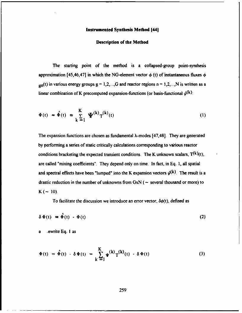
Instrumented Synthesis Method [441

Description of the Method

The starting point of the method is a collapsed-group point-synthesis

approximation [45,46,47] in which the NG-element vector 0 (t) of instantaneous fluxes 46

gn(t) in various energy groups g = 1,2,...,G and reactor regions n = 1,2,...,N is written as a

linear combination of K precomputed expansion-functions (or basis-functional 4Xk):

A K4'( - 4(0 ----k •=1 rk)k(t()

The expansion functions are chosen as fundamental X-modes [47,48]. They are generated

by performing a series of static critically calculations corresponding to various reactor

conditions bracketing the expected transient conditions. The K unknown scalars, T(k)(t),

are called "mixing coefficients". They depend only on time. In fact, in Eq. 1, all spatial

and spectral effects have been "lumped" into the K expansion vectors O(k). The result is a

drastic reduction in the number of unknowns from GxN (- several thousand or more) to

K(- 10).

To facilitate the discussion we introduce an error vector, 60(t), defined as

A

5 4(t) s ,I,(t) - 4(t) (2)

a ewrite Eq. I as

A K (k W4(t) = t(t) -(t) = , *i(k)T(k)(t) - 54(t) (3)

k=l1

259

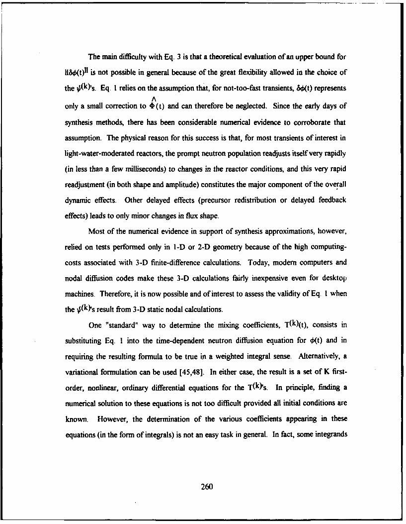
The main difficulty with Eq. 3 is that a theoretical evaluation of an upper bound for

l&•(t)ll is not possible in general because of the great flexibility allowed in the choice of

the 0(k)'s. Eq. 1 relies on the assumption that, for not-too-fast transients, W4(t) representsA

only a small correction to 4, (t) and can therefore be neglected. Since the early days of

synthesis methods, there has been considerable numerical evidence to corroborate that

assumption. The physical reason for this success is that, for most transients of interest in

light-water-moderated reactors, the prompt neutron population readjusts itself very rapidly

(in less than a few milliseconds) to changes in the reactor conditions, and this very rapid

readjustment (in both shape and amplitude) constitutes the major component of the overall

dynamic effects. Other delayed effects (precursor redistribution or delayed feedback

effects) leads to only minor changes in flux shape.

Most of the numerical evidence in support of synthesis approximations, however,

relied on tests performed only in 1 -D or 2-D geometry because of the high computing-

costs associated with 3-D finite-difference calculations. Today, modem computers and

nodal diffusion codes make these 3-D calculations fairly inexpensive even for desktop

machines. Therefore, it is now possible and of interest to assess the validity of Eq. 1 when

the #(k)s result from 3-D static nodal calculations.

One "standard" way to determine the mixing coefficients, T(k)(t), consists in

substituting Eq. 1 into the time-dependent neutron diffusion equation for 0(t) and in

requiring the resulting formula to be true in a weighted integral sense. Alternatively, a

variational formulation can be used [45,48]. In either case, the result is a set of K first-

order, nonlinear, ordinary differential equations for the T(k)s. In principle, finding a

numerical solution to these equations is not too difficult provided all initial conditions are

known. However, the determination of the various coefficients appearing in these

equations (in the form of integrals) is not an easy task in general. In fact, some integrands

260

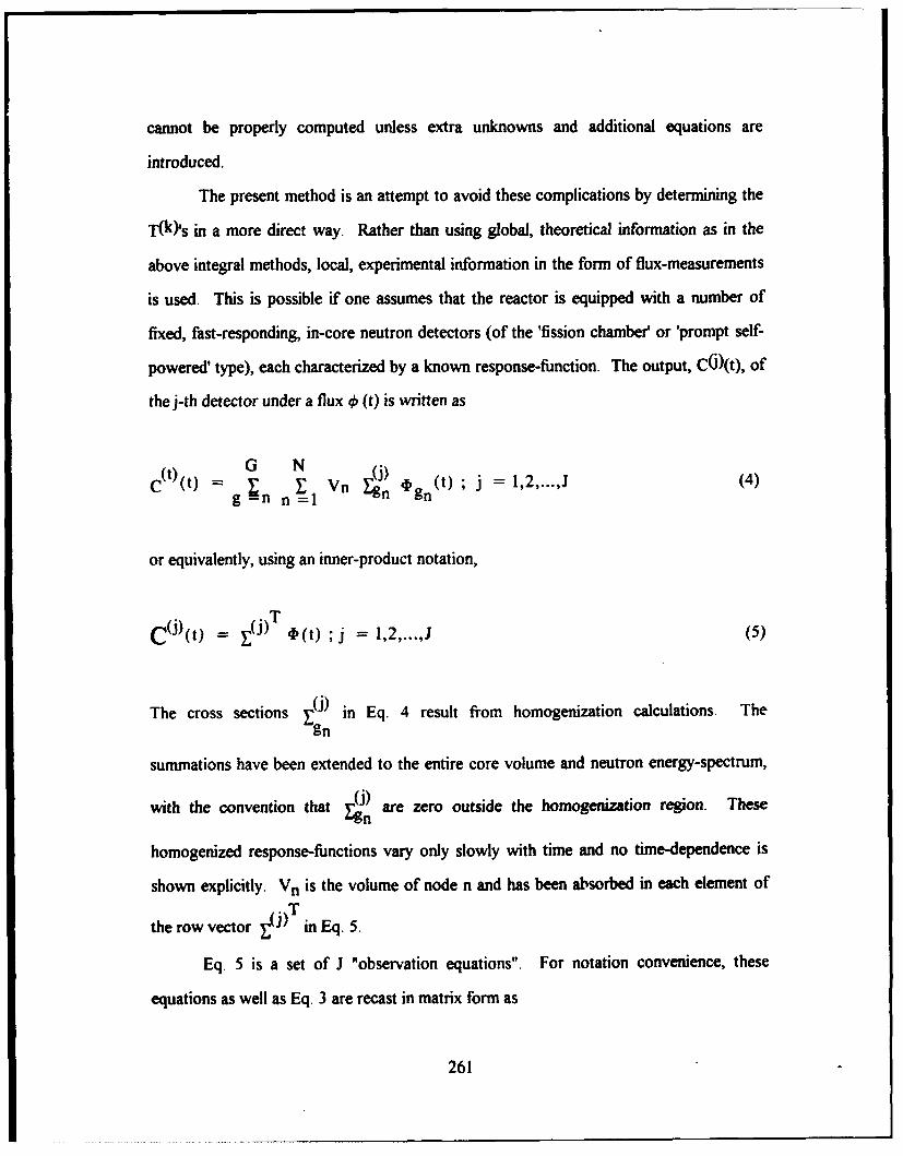
cannot be properly computed unless extra unknowns and additional equations are

introduced.

The present method is an attempt to avoid these complications by determining the

T(k)'s in a more direct way. Rather than using global, theoretical information as in the

above integral methods, local, experimental information in the form of flux-measurements

is used. This is possible if one assumes that the reactor is equipped with a number of

fixed, fast-responding, in-core neutron detectors (of the 'fission chamber' or 'prompt self-

powered' type), each characterized by a known response-function. The output, C()(t), of

the j-th detector under a flux 4, (t) is written as

W~)t G N WI 4gCn N *J) (t) ; j 1,2,...,J)g=n n -g

or equivalently, using an inner-product notation,

C'(t = t(t) ; j = ,2,...,J (5)

The cross sections 1(J) in Eq. 4 result from homogenization calculations. Thegn

summations have been extended to the entire core volume and neutron energy-spectrum,_(J)

with the convention that W are zero outside the homogenization region. These

homogenized response-functions vary only slowly with time and no time-dependence is

shown explicitly. Vn is the volume of node n and has been absorbed in each element of.T

the row vector •J) in Eq. 5.

Eq. 5 is a set of J "observation equations". For notation convenience, these

equations as well as Eq. 3 are recast in matrix form as

261

A

,(t) -, -5 ,(t) -*T(t) - f,(t) (6)

and

T'F T f(t) -= C(t) (7)

In the above matrix notation, i and Y are GN-by-K and GN-by-J rectangular matrices

respectively. Substitution of Eq. 6 into Eq. 7 yields

E T* T(t) - E T b(t) =-C(t) (8)

or simply

A T(t) + E(t) = C(t) (9)

where

TA my ET(10)

is a J-by-K matrix with positive entries (each entry is an inner product), and

E (t) -, T T6 4ý(t) (1

is a column vector of length J of systematic errors. If one assumes that the unknownA

error-vector 6 f (t) in Eq. 6 is small with respect to fI (t) (in the sense of some vector

262

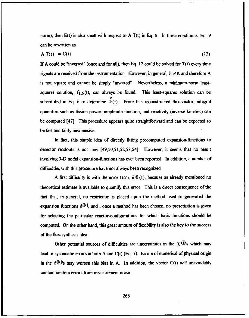
norm), then E(t) is also small with respect to A T(t) in Eq. 9. In these conditions, Eq. 9

can be rewritten as

A T(t) - C(t) (12)

If A could be "inverted" (once and for all), then Eq. 12 could be solved for T(t) every time

signals are received from the instrumentation. However, in general, J. #K and therefore A

is not square and cannot be simply "inverted". Nevertheless, a minimum-norm least-

squares solution, TLS(t), can always be found. This least-squares solution can beA

substituted in Eq. 6 to determine t (t). From this reconstructed flux-vector, integral

quantities such as fission power, amplitude function, and reactivity (inverse kinetics) can

be computed [47]. This procedure appears quite straightforward and can be expected to

be fast and fairly inexpensive.

In fact, this simple idea of directly fitting precomputed expansion-functions to

detector readouts is not new [49,50,51,52,53,54]. However, it seems that no result

involving 3-D nodal expansion-functions has ever been reported. In addition, a number of

difficulties with this procedure have not always been recognized.

A first difficulty is with the error term, 6 t (t), because as already mentioned no

theoretical estimate is available to quantify this error. This is a direct consequence of the

fact that, in general, no restriction is placed upon the method used to generated the

expansion functions 0(k), and , once a method has been chosen, no prescription is given

for selecting the particular reactor-configurations for which basis functions should be

computed. On the other hand, this great amount of flexibility is also the key to the success

of the flux-synthesis idea.

Other potential sources of difficulties are uncertainties in the Y (J)'s which may

lead to systematic errors in both A and C(t) (Eq. 7). Errors of numerical of physical origin

in the 0(k)'s may worsen this bias in A. In addition, the vector C(t) will unavoidably

contain random errors from measurement noise.

263

An additional, potentially serious, numerical problem arises from the fact that some

of the expansive functions, 0,(k), making up the columns of the matrix 0 may be almost

linear combinations of other expansion functions. As a result, the matrix A = E To may

be very ill-conditioned, i.e. almost rank-deficient. In some extreme cases, this ill-

conditioning may lead to a least-squares solution of Eq. 12 which is completely

meaningless because of roundoff-error amplification. The same problem may arise from

row-redundancies when only a reduced number of detectors is used with symmetries both

in their locations and in the core composition pattern.

264

Documents

CHARLES STANLEY LASOTA - DTIC · CHARLES STANLEY LASOTA S ,AUGU• 3 191 B.S., Electrical Engineering University of Kansas, 1985 Submitted to the Departments of Nuclear Engineering