Embed Size (px)
Citation preview

Characterizing the IEEE 802.11 Traffic: TheWireless Side
Jihwang Yeo, Moustafa Youssef, Ashok AgrawalaDepartment of Computer Science
University of MarylandCollege Park, MD 20742�
jyeo,moustafa, agrawala � @cs.umd.edu
CS-TR-4570 and UMIACS-TR-2004-15March 1, 2004
Abstract— Many studies on measurement and characterizationof wireless LANs have been performed recently. Most of thesemeasurements have been conducted from the wired portion ofthe network based on wired monitoring or SNMP statistics. Inthis paper we argue that traffic measurements from a wirelessvantage point in the network are more appropriate than wiredmeasurements or SNMP statistics, to expose the wireless mediumcharacteristics and their impact on the traffic patterns. While itis easier to make consistent measurements in the wired part ofa network, such measurements can not observe the significantvagaries present in the wireless medium itself. As a consequenceconstructing an accurate measurement system from a wirelessvantage point is important but usually quite difficult due to thenoisy wireless channel. In our work we have explored the variousissues in implementing such a system to monitor traffic in anIEEE 802.11 based wireless network. We show the effectivenessof the wireless monitoring by quantitatively comparing it withSNMP and measurements at wired vantage points. We also showthe analysis of a typical computer science department networktraffic using the wireless monitoring technique. Our analysisreveals rich information about the PHY/MAC layers of the IEEE802.11 protocol such as the typical traffic mix of different frametypes, their temporal characteristics, correlation with the useractivities and the error characteristics of the wireless medium.Moreover, we identify anomalies in the operation of the IEEE802.11 MAC protocol. Our results show excessive retransmissionsof some management frame types reducing the useful throughputof the wireless network. We also find that some features ofthe protocol, which were designed to reduce the retransmissionerrors, are not used. In addition, most of the clients fail to adaptthe data rate according to the signal condition between them andthe access point, which further reduce the useful throughput.
I. INTRODUCTION
With the popularity of the IEEE 802.11 [1] based wirelessnetworks, it has become increasingly important to understandthe characteristics of the wireless traffic and the wirelessmedium itself. A number of measurement studies [2]–[7] haveexamined traffic characteristics in wireless networks. In thesestudies, the measurements have been conducted on the wiredportion of the network and/or combined with SNMP logs [2].
The measurements at such wired vantage points can pro-vide accurate traffic statistics as seen in that portion of thenetwork. However they are mostly unable to expose the wire-
Wireless MonitoringWireless
Monitoring
Access Point
Ethernet
LA
N
Access Point
Wired Monitoring
Wired Monitoring
SNMPQuery
SNMPQuery
WAN
CollectingSNMP DataCollecting
SNMP Data
Fig. 1. Monitoring Wireless Traffic: from a wired vantage point, a wirelessvantage point, and SNMP statistics.
less medium characteristics (PHY/MAC in the IEEE 802.11)because they cannot observe the actual IEEE 802.11 frameson the air.
SNMP [16], [17], [19] can be analyzed to give aggregatestatistics about the IEEE 802.11 wireless LAN (WLAN) fromthe access point (AP) perspective. Such information includesthe number of erroneous frames and reasons for most recentlydisassociated stations, etc. They provide accurate traffic sizeinformation at Access Points [16], [17]. However this infor-mation is either aggregate (e.g. Frame Count) or instantaneousinformation (e.g. last Disassociated Station) that depends onthe polling interval (typically order of minutes). Thereforethey hardly represent complete frame-by-frame statistics norrepresent the statistics from the client point of view.
In this paper, we introduce wireless monitoring as a trafficcharacterization technique. Rather than looking at part of thepicture through wired monitoring and/or SNMP statistics, we

argue that traffic measurements from a wireless vantage pointin the network are crucial to analyzing the full picture ofthe 802.11 wireless network. We show that not only doeswireless monitoring give the same information provided bywired monitoring and SNMP statistics, but it also providesmuch richer information about the wireless medium.
Fig. 1 illustrates “wired monitoring”, a measurement froma wired vantage point, and “wireless monitoring”, a measure-ment from a wireless vantage point, and SNMP statistics.
We believe that our study is the first to expose thePHY/MAC characteristics of the IEEE 802.11 traffic and to ob-tain more detailed error statistics than studies based on wiredmonitoring or SNMP statistics alone. Therefore, our workpresents a basis for building models and simulation tools ofthe 802.11 wireless networks. Moreover, our detailed analysisof the wireless medium allowed us to identify anomalies in theoperation of the IEEE 802.11 MAC protocol that have a largeimpact on the network throughput (Section V). This studywould help protocol designers and manufacturers to refinethe protocol and implementation to remove the anomaliesidentified.
We have performed a detailed passive measurement experi-ment over a period of two weeks, in which we have observedthe wireless PHY/MAC characteristics in the A.V. Williamsbuilding on the campus of University of Maryland, whichhouses the Department of Computer Science. The wireless net-work in this building has a high traffic load. Our observationsindicate that indeed a consistent inference based on a wirelessmeasurement is possible. However, the measurement processis significantly more challenging than when performed from awired vantage point.
A. Advantages of Wireless Traffic Monitoring
The wireless monitoring system consists of a set of deviceswhich we call sniffers, to observe traffic characteristics onthe wireless medium. Wireless monitoring is more useful forunderstanding the traffic characteristics in wireless network forthe following reasons.
A wireless monitoring system can be set up and put intooperation without any interference to existing infrastructure,e.g. end-hosts and network routers. In fact wireless monitoringcan be performed without any interaction with the existing net-work, and hence is completely independent of the operationalnetwork.
More importantly, wireless monitoring exposes the charac-teristics on the wireless medium itself so that we can infer thePHY/MAC characteristics. Thus wireless monitoring allowsus to examine physical layer header information includingsignal strength, noise level and data rate for individual packets.Similarly it also enables examination of the link layer headers,which include IEEE 802.11 type and control fields [1]. This isnot possible with the measurements at a wired vantage point.Compared to SNMP logs, wireless monitoring allows us tohave detailed information about all stations, while in SNMPlogs only the aggregate or instantaneous information as seenfrom the AP view are available.
Physical layer information can be used to see how theycorrelate with error rates and throughput. This is useful fordeveloping accurate error models for the IEEE 802.11 WLANsand in site planning to determine the minimum signal strengthrequired to achieve a certain throughput or error rate.
By analyzing the link layer data, we can characterize trafficaccording to different frame types, namely: data, control, andmanagement frames.
The collected data, combined with timestamps, can be usedas accurate traces of the IEEE 802.11 link-level operations.Such traces are useful when we want to emulate the protocolor diagnose problems of wireless networks.
Several throughput models [8], [9] on the IEEE 802.11 havebeen introduced, which propose collision rate, transmissionrate and throughput as important performance metrics. Wire-less monitoring enables us to make exact measurement of suchIEEE 802.11 MAC-level performance metrics.
B. Challenges of Wireless Monitoring
The advantages we mentioned above, however, would not beexploited unless the sniffers can capture nearly all the frameson the air. Unfortunately it is very difficult to guarantee thatany sniffer can capture all such wireless frames. We haveobserved that typically most of these losses are due to signalstrength variability, card variability or a combination of both.Losses in the sniffers pose the most challenging problem inwireless monitoring.
If sniffer losses are inevitable, then the following questionscan be raised. How can we reduce such sniffer losses? How canwe justify that even with such losses the measurement providesmeaningful results, consistent with the end-to-end real worldexperiences? In order to answer these questions, we conducteda controlled experiment using an end-to end measurement toolas a baseline for accuracy. In Section III we present the resultsfor this experiment that helped us identify the pitfalls that awireless measurement system needs to be aware of. We alsopresent the techniques that can be used to avoid them. Thesetechniques can be used in future wireless monitoring-basedexperiments.
C. Organization
The rest of the paper is organized as follows. In Section IIwe discuss previous works in the area of WLAN traffic charac-terization. Section III describes the controlled experiment, thepitfalls of wireless monitoring, techniques to overcome them,and how wireless monitoring compares to wired monitoringand SNMP statistics. We describe the results of our two-weeklong experiment in Section IV. In Section V we discuss theanomalies we discovered in the 802.11 implementations andthe traffic characterization. Finally, we conclude the paper inSection VI and highlight our ongoing work.
II. RELATED WORK
Several measurement and analysis studies [2]–[4], [7], [11]have examined traffic or error characteristics in the IEEE

802.11 WLAN. Most of the measurements have been per-formed on university WLAN [3], [4], [7], [11], while the workin [2] examined WLAN traffic in a conference environment.
The study of Tang and Baker [4] in the Computer ScienceDepartment building of Stanford University was one of theearly studies. They examined wired monitoring traces, andSNMP logs to analyze a twelve-week trace of a local-areawireless network.
In a public-area wireless network, the traces collected inwell-attended ACM conference were successfully analyzed byBalachandran et al. [2]. They used SNMP logs and wiredmonitoring to characterize not only the patterns of WLANusage, but also the workloads of user arrivals and session dura-tions with parameterized models. They also analyzed channelcharacteristics using SNMP logs and presented aggregate errorpercentages from the AP point of view.
A significantly larger scale experiment covering a muchlonger duration and coverage area has been presented in theDartmouth campus by Kotz and Essien [3]. Their analysis wasbased on using system logs in APs, SNMP logs and wiredmonitoring traces to characterize the typical usage and trafficpatterns in a university WLAN.
In a similar recent study, Schwab and Bunt [7] used wiredmonitoring and the Cisco proprietary LEAP authenticationlogs to characterize one-week usage and traffic patterns in acampus-wide WLAN environment.
Similar to the previous studies, our measurements areperformed on typical university WLAN environment in adepartment network. We are interested in showing the trafficcharacteristics for a typical access point in this environment.Our uniqueness comes from analyzing the wireless mediausing the wireless monitoring technique which gives a fullview of the network spanning all the layers of the protocolstack. In all the above studies the measurements have limitedanalysis of the PHY/MAC layer based on the aggregate dataof the SNMP traces.
In a more general wireless environment, the authors in [5],[6] performed wireless monitoring to measure packet lossand Bit Error Rate. Their experiments were fully controlledbetween two wireless stations and performed on non-802.11networks. Our work is different in being in the context of802.11 WLANs and in performing the experiment in an actualenvironment with different goals.
III. CONTROLLED EXPERIMENT
In this section, we present our controlled experiment. Thepurpose of this experiment is to analyze the wireless mon-itoring technique in terms of its effectiveness in capturingwireless traffic and presenting precise statistics for wirelessmedium. Moreover, we compare its performance to that ofwired sniffing and SNMP statistics. Since only the wirelessmonitoring provides detailed information about the PHY/MAClayer, we base our comparison in this section on the percent-age of frames that can be captured by different techniquescompared to the frames generated by a reference application.
Source
NetDyn
Sink
Echo
NetDynSrc SeqNum
Src SeqNum Echo SeqNum
NetDyn Processes Packets
Src SeqNum Echo SeqNum
Fig. 2. NetDyn processes and their sequence numbers.
For more detailed description of our controlled experimentsreaders are recommended to refer to Appendix II.
A. Methodology
1) Network Infrastructure: We perform our experimentsin the A.V. Williams building, at University of Maryland(where the Department of Computer Science is located). Thebuilding has 58 access points installed, which belong to threedifferent wireless networks. Each wireless network is identifiedwith its ESSID. The ESSIDs of the three networks are umd,cswireless and nist respectively. umd network consists of 29Cisco Aironet A-340 APs, the most widely used wirelessnetwork in the university. cswireless (12 Lucent APs) andnist (17 Prism2-based APs) are built by individual researchresearch groups in the department1.
We performed our controlled experiment on a separatenetwork that we set up specifically for this purpose with itsown ESSID. Our clients were configured to associate with thisAP.
2) NetDyn: To estimate the exact measurement loss, weneed to use reliable application generated sequence numbers.We conducted a two-way UDP packet exchange experimentsusing an end-to-end traffic measurement tool, called NetDyn[13].
As shown in Fig. 2, NetDyn consists of three differentprocesses, Source, Echo and Sink. Source puts a sequencenumber in the payload, sends the packet to Echo, which alsoadds a sequence number before forwarding it to Sink. In oursetup, Source and Sink processes run on a wireless station,while the Echo process runs on a server wired to the LAN.Using the sequence numbers generated by the Source and Echoprocesses, we can determine which packets were lost in thepath from the Source machine to the Echo machine and viceversa.
In the experiment, Source sends 20000 packets with thefull UDP payloads (1472 bytes) to Echo, with 10 ms inter-packet duration (hence, at 100 packets/second). We madesure that no fragmentation occur on either side of the AP.
1All networks mentioned in the paper are based on the 802.11b protocol.

Therefore, for each NetDyn frame on the wireless side, thereis a corresponding frame on the wired side and vice versa. Weuse the NetDyn statistics as the baseline for comparison withother monitoring techniques.
3) Monitoring Hardware/Software: We set up three sniffermachines to capture the wireless frames on the air. Allsniffing devices use the Linux operating system with kernelversion 2.4.19. We used Ethereal (version 0.9.6) and libpcaplibrary (version 0.7) with the orinoco cs driver (version 0.11b),patched to enable monitoring mode, as our sniffing software.We made use of the ‘monitor mode’ of the card to capture802.11 frame information including the IEEE 802.11 headeras well as physical layer header, called the Prism2 monitorheader, and higher layer protocols’ information.
A wired sniffer was installed on the same LAN as the APand the NetDyn Echo machine through a Century Tap, a full-duplex 10/100 Ethernet splitter [20]. The sniffer machine wasrunning Ethereal. The same machine was running the SNMPclient that was configured to poll the AP for SNMP statisticsevery one minute.
4) Captured Wireless Data : The wireless sniffer capturesthe first 256 bytes of each receiving 802.11 frame, records thecomplete view of the frame, i.e. PHY/MAC/LLC/IP/Above-IPinformation.
Prism2 monitor header is not a part of IEEE 802.11 frameheader, but is generated by the firmware of the receiving card.The header includes useful PHY information, such as MACTime, RSSI(Received Signal Strength Indication), SQ (SignalQuality), Signal strength, Noise and Signal Noise Ratio (SNR)and Data rate (in Mbps). All signal and noise information arein manufacture-specific units. However, they can be used forrelative comparison.
We also capture the IEEE 802.11 MAC frame structurewhich incorporates the following fields: protocol version,frame type (management, data and control), Duration forNetwork Allocation Vector (NAV) calculation, BSS Id, Sourceand Destination MAC addresses, fragment, sequence numberamong others [1]. According to the 802.11 MAC frame typeof the captured frame, we extract different information. Forexample, for Beacon frames, captured information include 64-bit Beacon timestamp which we use for time synchroniza-tion among multiple sniffers (Section III-C). For Associa-tion/Disassociate and Authentication/Deauthentication frames,the information includes the reason code for such actions.
We also capture higher layer protocol information, mainlyfor NetDyn frames.
For SNMP, we can capture the same statistics as in [2]. Forwired sniffer data, we capture enough information to give usthe NetDyn sequence numbers.
5) Experiment Setup: We tried different scenarios for thetraffic between the wireless clients and the wired server. Inthe rest of this section we show the results of one experimentwhose configuration is shown in Fig.3. Other configurationsgave comparable results. We have two wireless clients attwo different locations corresponding to two different signalconditions. The “Good” client lies in an area of good AP
Access Point
Ethernet L
AN
Sniffer
Source
NetDyn
Sink
NetDyn
Echo
Source
NetDyn
Sink
SnifferSniffer
Wired sniffer
snmputil
20000 UDP packets
20000 UDP packets
Fig. 3. Controlled Experiment using NetDyn: Source in a wireless stationsends 20000 UDP packets to wired Echo machine which sends them back toSink in the same wireless station.
��
��
��
��
����
��
��
��
������
���
���
�
�
�� �
���������������
� �����������
�����
������
��
Fig. 4. SNR Contour Map for controlled experiment: SNR Contour linesfor 40,30,20 and 15 dB are obtained from SNR measurements. Based on thecontour map, we place the wireless clients at locations G and B and placethe sniffers at locations T, U, and V.
coverage, in terms of SNR, while the “Bad” client lies in anarea of bad AP coverage. We also have three wireless sniffers(T, U and V) capturing the wireless traffics between Source,Sink and the AP. Sniffer T is placed adjacent to the AP whilethe other two sniffers are placed as shown in Fig.342. Note thatthe purpose of placing the sniffers in the controlled experimentwas not to maximize the capture performance, but rather tostudy the different factors affecting the wireless monitoringperformance.
B. Single Sniffer Statistics
We define a “From-AP” frame, as a frame transmitted by theAP to a wireless station. Similarly, we refer to a frame from thewireless station to the AP as a “To-AP” frame. Table I showsthe number of received packets for the NetDyn application andthe percentage of MAC frames captured by the three wirelesssniffers. We define the measurement loss to be the percentageof the frames unobserved by the sniffer.
2We discuss sniffers placement in Section III-D.

The entries for the wireless sniffers were obtained bycounting all frames with unique sequence numbers. We canmake the following observation from the table:� Different sniffers have different viewpoints of the wire-
less medium.� The percentage of measurement loss for From-AP trafficis much less than the percentage of measurement lossfor To-AP traffic. On the average, one sniffer can see99.4% for From-AP traffic and 80.1% for To-AP traffic.The reason for that is that the AP has better hardwarecompared to clients, therefore the signal seen at a snifferfrom an AP is stronger than the signal seen from a client.Moreover, we can always place a sniffer adjacent to anAP , whose position is fixed, while we cannot do that forwireless clients as their position is not known in advance.� Each sniffer has a significant percentage of unobservedframes compared to NetDyn data. Even sniffer T, whichwas placed adjacent to the AP, encountered a severemeasurement loss to observe only 73% of the total traffic.These measurement losses may be due to signal strengthvariability, card variability or a combination of both.� The absolute physical location of the client or the snifferdoes not affect the ability of a particular sniffer to capturedata from a particular wireless client. Rather, the relativeposition between the wireless client and the sniffer isthe factor that affects the ability of a sniffer to capturethe data from that client. For example, for the trafficoriginating from Bad client, sniffers U and V capturemore traffic than sniffer T. The reason for that is as thedistance from the sniffer to the wireless client increases,the signal strength decays and the SNR decreases leadingto worse signal conditions and decreased sniffing perfor-mance. Sniffers U and V are closer to Bad client thansniffer T.� In Bad client case, the sniffers captured some framesthat was not received by the NetDyn application (capturepercentage � 100%). This is because all sniffers arecloser to the AP than Bad client which means that aframe sent by the AP will have a better SNR at thesniffer compared to Bad client. Therefore, the snifferscan capture frames that Bad client cannot capture.
From these observations we can see that two factors areimportant to achieve a good capture percentage, i.e. a lowmeasurement loss, from wireless monitoring:
1) Merging the data collected from different sniffers toobtain a better view of traffic.
2) Carefully selecting the sniffers location to obtain anacceptable capturing performance.
We address the two factors in the next sections. Moreoverwe introduce two techniques for improving the performanceof wireless monitoring, namely merging multiple sniffers andsniffer placement. We briefly describe those techniques in thefollowing sections. For more detailed description of thosetechniques, readers are recommended to refer to Appendix I.
C. Merging Multiple Sniffer Data
The main problem that needs to be tackled in order to mergethe data from different sniffers is how to synchronize the traceswhen each of them is time-stamped according to the localclock of the sniffer. In this section, we describe our methodfor time synchronization, merging procedures and the effectof merging respectively.
1) Time Synchronization between Multiple Traces : Tocorrectly merge multiple sniffers’ data without reordering werequire the time synchronization error (the difference betweentwo timestamps of different sniffers for the same frame) to beless than the minimum gap between two valid IEEE 802.11frames. In the IEEE 802.11b protocol, the minimum gap,�����
, can be calculated as the 192 microsecond preambledelay plus 10 microsecond SIFS (Short Inter-Frame Space), atotal of 202 microsecond.
Our approach is to use the IEEE 802.11 Beacon frames,which are generated by the AP, to be the common frames to allthe sniffers. Beacon frames contain their own 64-bit absolutetimestamps as measured by the AP, therefore we can uniquelyidentify such common beacon frames in different sniffer traces.With such � common beacon frames, we then take one of thesniffers as a reference point and use linear regression to fit theother sniffers’ timestamps 3 to the reference sniffer.
Fig. 33 shows the fitting error (difference between thefitted timestamp and the reference timestamp) for the commonBeacon frames over a 12.5 minutes interval. During thisperiod, there were 5658 Beacon frames that were commonto all the sniffers out of the total of the 7500 total Beaconsframe that are sent at the 100 ms rate. Sniffer T was taken asthe reference sniffer in this experiment. We can see that themaximum error is below 40 microseconds, well below the 202microseconds limit.
2) Merging Procedures : Using the obtained linear equa-tion, we can convert the timestamp of each frame captured byeach sniffer, to the reference time. To identify the duplicateframes that multiple sniffers commonly observed, we comparethe header information of the frames, which are from differentsniffer traces and whose converted timestamps differ by lessthan the minimum gap
� ����. After removing the duplicates,
we can generate a single correctly-ordered trace from multiplesniffer traces.
3) The Effect of Merging : Table I shows the effect of usingthe merged sniffers’ traces. We can see from the table thatincreasing the number of merged sniffers’ traces from oneto two to three increases the percentage of captured framessignificantly from 73.25% to 84.47% to 99.34% respectivelyfor the To-AP traffic. Notice also that the effect of mergingis more significant in the case of To-AP traffic while a singlesniffer near the AP (sniffer T) can almost capture all the From-AP traffic (improvement from T only to T+U+V is 0.7%).
3We use the MAC time of the received frame, which is available in Prism2header in the captured frame, as the local timestamp at each machine. We donot use the timestamp generated by the sniffer’s operating system to minimizethe variance of the local time measurement.

-60
-40
-20
0
20
40
60
0 1 2 3 4 5 6 7 8 9 10 11 12
Fitti
ng E
rror
(µse
c)
Elapsed Time(minutes)
Sniffer TSniffer USniffer V
Fig. 5. Fitting error with 5658 common Beacon frames (timestamp of snifferT is the reference time).
Using the merged three-sniffers ’ trace, wireless monitoringcan capture more than 99.34% of the wireless traffic.
D. Sniffers Placement
As noted in Section III-B, carefully selecting the snifferslocation is important to obtain an acceptable capturing per-formance. In this section, we describe our sniffer placementstrategy in the coverage area of an AP . We make use of theobservations presented in Section III-B.
Since in the infrastructure mode of the 802.11 protocol alltraffic goes through the AP, one may think that placing allsniffers near the AP should maximize the capture performance.However, our experiments showed that the capture perfor-mance of To-AP traffic is worse than that of the From-APtraffic, even for the sniffer T which was adjacent to the AP.This is due to the weak signal that reaches the sniffer fromthe clients compared to the strong signal that reaches the samesniffer from the AP. The AP can capture the weak signal dueto its better hardware and specialized processing (compared tothe sniffer configuration).
Therefore, for placing the wireless sniffers, we should onlyplace one sniffer adjacent to the AP to be responsible forcapturing the From-AP traffic and the traffic of clients nearthe AP. Other sniffers should be placed as close as possibleto the wireless clients.
If we assume that clients are going to be uniformly dis-tributed over the coverage area, this translates to placing thesniffers so that they cover as much as possible from the APcoverage area. Therefore, if we have � sniffers to place, wecan split the AP coverage area into � equal areas and placethe sniffers in the center of mass of these areas.
We can refine this strategy by noting that, in an environmentwhere multiple APs are installed, the coverage area of anAP may be reduced to the Association Area of the AP. TheAssociation Area of an AP is the area at which a client willfavor this AP for association compared with other APs inthe area. Note that the Association area is a sub-area of thecoverage area and that most of the traffic an AP receives comes
AP1
AP7
Border between association areas for different APs
AP2
AP3
AP4
AP6
AP5
Border for the coverage area for AP1
Fig. 6. The Association Area for different access points. The figure alsoshows the coverage area for the first access point.
TABLE IIITOTAL NUMBER OF RETRANSMISSIONS
To-AP From-APWireless Wireless MIB-I MIB-II
Good 576 386 N/A N/ABad 5121 4181 N/A N/ATotal 5697 4567 3007 4874
from the associated clients (i.e. from the Association Area).Therefore, we should use the association area of an AP ratherthan its coverage area. Fig. 6 shows the Association Areasfor different access points in the area of interest. The figurealso shows the difference between the coverage area and theassociation area for ����
Another factor that needs to be taken into account is thesignal condition at the sniffer location. We define an SNR wallas an area where the SNR contour lines are close to each other(Fig. 34). Our experiments shows that placing a sniffer nearan SNR wall leads to worse capture performance comparedto placing the sniffer at other places. Therefore, SNR wallsshould be avoided.
E. Comparison Between Different Characterization Tech-niques
Tables XI and III show a comparison between the threetraffic characterization techniques taking NetDyn results as thebaseline. Note that for SNMP statistics, we based our analysison MIB-I counters as in [2] and on the MIB-II counters.
From the table, we can make the following observations:� Wireless monitoring has comparable performance to theother techniques for the common information that can becaptured by other techniques.� SNMP statistics cannot reveal per client information.� Wired monitoring can give accurate To-AP informationabout the wireless medium for the successfully transmit-ted frames as the probability of the loss on the wiredmedium is order of magnitudes less than the probabilityof loss on the wireless medium. However, if the frames

TABLE IINCREASING CAPTURED FRAMES BY MERGING MULTIPLE SNIFFERS: MERGING TWO OR THREE SNIFFERS AMONG T, U AND V SIGNIFICANTLY
INCREASES THE NUMBER OF OBSERVED FRAMES.
To-AP Wireless TrafficNetDyn T U V T+U T+V U+V T+U+V
Good 19905 76.76% 69.00% 68.34% 76.83% 70.00% 76.84% 98.61%Bad 18490 69.48% 99.58% 99.73% 99.05% 100.05% 99.97% 100.13%Total 38395 73.25% 83.73% 83.46% 87.54% 84.47% 87.98% 99.34%
From-AP Wireless TrafficGood 19247 98.41% 97.31% 95.24% 99.37% 98.06% 99.32% 99.38%Bad 17858 102.04% 101.85% 102.2% 102.56% 102.43% 102.52% 102.56%Total 37105 100.15% 99.5% 98.59% 100.91% 100.16% 100.86% 100.91%
TABLE IIQUANTITATIVE COMPARISON BETWEEN END-TO-END MEASUREMENT USING NETDYN, SNMP, WIRED MONITORING AND WIRELESS MONITORING
To-AP Wireless TrafficNetDyn Wireless Monitoring (%) Wired Monitoring (%) MIB-I (%) MIB-II (%)
Good 19905 98.61 100.00 N/A N/ABad 18490 100.13 100.00 N/A N/ATotal 38395 99.34 100.00 100.23 100.23
From-AP Wireless TrafficGood 19905 99.38 103.41 N/A N/ABad 18490 102.56 103.53 N/A N/ATotal 38395 100.91 103.47 102.02 99.96
are fragmented on the wireless medium, we cannot getcorrect statistics on the wireless frames from the wiredside.� For the From-AP traffic, although wired monitoring cangive per client information for the wired segment, itsstatistics overestimates the actual traffic more than thewireless monitoring technique. The reason for that is thenoisy characteristic of the wireless channel that leads tothe loss of many packets on the wireless side that wiredmonitoring cannot capture.� Only wireless monitoring can capture the retransmissioninformation per client.� Wireless monitoring is more accurate than the MIB-Ibased method that was used in [2] in characterizing thenumber of retransmissions.� It is interesting to notice that even the SNMP statisticsmay be slightly off from the true image of the wirelessclient. For example, in Table XI the MIB-II total numberof successfully transmitted packets is less than the num-ber of packets received by the NetDyn Sink. This canbe explained by noting that there may be packets thatwas successfully received by the NetDyn Sink after threeretransmissions and the corresponding MAC-level ACKsent back. However, the ACK was not received by the APand the AP did not count it as a successful transmission.
What we are trying to argue here is that wireless monitoringhas comparable performance to the other techniques but has
the advantage of exposing the full wireless medium frames.The next section shows the characterization for the traffic in acomputer science department environment for a period of twoweeks based on the wireless monitoring.
For more detailed results and discussions on the comparison,readers are recommended to refer to Appendix III.
IV. WIRELESS TRAFFIC CHARACTERISTICS: ANALYSIS OFTWO-WEEK TRACES
We apply the wireless monitoring technique to measureand characterize actual wireless LAN traffics of a typicalAP in a computer science department network. We haveperformed passive measurements over a period of two weeksfrom Monday, February 9 to Sunday, February 22 to observethe wireless PHY/MAC characteristics in the fourth floor ofthe A.V. Williams building of Department on the campus ofUniversity of Maryland.
A. Methodology
1) Target Traffic: In the fourth floor of A.V. Williamsbuilding, we have three channel-6 APs, three channel-1 APsand one channel-1 AP. Channel 6 is the most widely used inthe fourth floor, therefore we choose channel 6 as our targetchannel. We choose one of the channel-6 APs in the fourthfloor as our target AP. We can monitor the traffics of both thetarget AP and the channel 6 at the same time, because oncewe set the sniffers’ channel to 6, then the sniffers capture allthe observed traffic on the channel (and adjacent overlapping

M9 T10 W11 T12 F13 S14 S15 M16 T17 W18 T19 F20 S21 S220
5
10
15
20
25
30
35
40
45
Days
Num
ber o
f Fra
mes
per
Sec
ond
AllDataMgmt
Fig. 7. [MAC Traffic] Number of MAC frames per seconds, averaged daily,over two weeks: All traffic of the target AP is the sum of MAC Data trafficand Mgmt (Management) traffic.
channel). Due to space constraints, we only show the trafficanalysis for one AP in this paper.
2) Setup and Placement: The setups for H/W and S/W inthree sniffers are exactly the same as in controlled experimentin Section III. We also followed our strategy for snifferplacement as discussed in the Section III-D. Sniffer T is thesniffer placed adjacent to the target AP.
3) Trace Collection: We started the wireless monitoringat midnight, Monday February 9, ended at midnight, SundayFebruary 22, for a total of 14 days.
The size of the three trace files, which are generated byEthereal, is in total 12 GB in compressed format. We hada gap of 8 hours, noting that unfortunately from 4:00 pm to11:59 pm on February 20, we were unable to capture the trafficdue to disk fullness of three sniffer machines. On that day,traffic volume of channel 6 became tremendously higher thanexpected.
B. Results
We focus our presentation on the characterization ofPHY/MAC layer traffics, which is unique to wireless moni-toring. Specifically we will present our results under five cat-egories: MAC Traffic, Transmission Errors, MAC Frame Types,MAC Frame Size and PHY Information. We also summarizethe anomalies we discovered at the end of the section.
1) MAC Traffic: Fig. 7 and Fig. 8 show the daily trafficover the two weeks. We obtain MAC type and size informationfrom each frame’s MAC header in the traces. We separatelypresent traffic for IEEE 802.11 Data frames and that for theIEEE 802.11 Management frames (e.g. Beacon and ProbeRequest frames).4
We notice that there was almost no user activity on theweekend of Feb. 14 and Feb. 15. This weekend represents the
4Since the IEEE 802.11 control frames (e.g. Acknowledgement) have noBSSID, i.e. MAC address of AP, we do not present the results for the controlframes in this section.
M9 T10 W11 T12 F13 S14 S15 M16 T17 W18 T19 F20 S21 S220
0.2
0.4
0.6
0.8
1
1.2
1.4
1.6
1.8
2x 10⁴
Days
Byt
es p
er S
econ
d
AllDataMgmt
Fig. 8. [MAC Traffic] Traffic volume per seconds. Daily averaged valuesare shown over two weeks: All traffic of the target AP is the sum of MACData traffic and Mgmt (Management) traffic.
0 2 4 6 8 10 12 14 16 18 20 22 240
50
100
150
200
250
Hours
Num
ber o
f Fra
mes
per
Sec
ond
Feb. 18Feb. 11
2 frames per second
Fig. 9. [MAC Traffic] Number of IMAP frames per second. Plot showshourly averaged values on February 18 and on February 11 respectively.
weekend for Valentine’s Day. February 16 was the holiday forPresident’s Day. However, the university is open in that day.
Typically traffic for the IEEE 802.11 Management framesis constant over the two weeks period. On Friday, February20, disk space had been full for 8 hours therefore we havesmaller number of frames than normal days (about one thirdof the normal management traffic volume).
We observe a sudden spike of traffic on Wednesday, Febru-ary 18, which is three times larger than normal days. Carefullyexamined, we found that 40% of MAC Data traffic consistsof IMAP (Internet Message Access Protocol) frames. IMAPprotocol is used when client STA accesses electronic mail orbulletin board messages that are kept on a (possibly shared)mail server [21].
In other days, for example on another Wednesday, February11, the traffic contains IMAP frames less than 1% (Figure 9).

M9 T10 W11 T12 F13 S14 S15 M16 T17 W18 T19 F20 S21 S220
5
10
15
20
25
Days
Num
ber o
f Fra
mes
per
Sec
ond
From−APTo−AP
Fig. 10. [MAC Traffic] Number of Data frames per second. Daily averagedvalues are presented over two weeks.
M9 T10 W11 T12 F13 S14 S15 M16 T17 W18 T19 F20 S21 S220
2000
4000
6000
8000
10000
12000
14000
16000
18000
Days
Byt
es p
er S
econ
d
From−APTo−AP
Fig. 11. [MAC Traffic] Traffic volume per second for Data frames. Dailyaveraged values are presented over two weeks.
This abnormal spike of email traffic is due to email wormW32.Netsky.B � mm that was spreading on the web on Feb. 18[24].
Another observation from figures 7 and 8 respectively isthat the maximum throughput (in bytes per second) does notexceed 1.5 Mbps (Megabits per second). This low throughputcan be explained by noting that there are 2 other APs assignedto channel 6 in our environment. These APs along with theclients associated with them, contended for the same channelwith our target AP, hence reduced the throughput. We believethat this multiple-APs assignment to the same channel is atypical real world scenario.
We present the number of frames per second and the trafficvolume, in bytes, for the Data traffic only in Fig. 10 andFig. 11 respectively. We can observe that From-AP traffic andTo-AP traffic show the same shape, which means that mostof the traffic consists is two-way pairs, e.g. Request/Responseinteractions. For the number of frames per second, From-AP
0 2 4 6 8 10 12 14 16 18 20 22 240
5
10
15
20
25
30
35
40
45
50
Hours
Num
ber o
f Fra
mes
per
Sec
ond
AllDataMgmt
Fig. 12. [MAC Traffic] Number of frames per second. Plot shows hourlyaveraged values over two weeks.
0 2 4 6 8 10 12 14 16 18 20 22 240
0.5
1
1.5
2
2.5
3x 10
4
Hours
Byt
es p
er S
econ
d
AllDataMgmt
Fig. 13. [MAC Traffic] Traffic volume per second. Plot shows hourlyaveraged values over two weeks.
traffic has on average five times many frames than To-APtraffic. In addition, the bytes per second of From-AP traffic areroughly 12 times larger than To-AP traffic, on average. Thisbehavior is expected as most requests are short (e.g. HTTPGet request) while the responses are larger in general.
Fig. 12 and Fig. 13 show hourly traffic variability, averagedhourly over two weeks. We can observe that the traffic has twopeaks at 11 am and 6 pm. However, the peak at 6 pm is dueto the abnormal high traffic volume on Feb. 18. During lowuser traffic periods, from about 8pm and 8am, Managementframe traffic is dominant.
Fig. 14 and Fig. 15 show hourly traffics of the IEEE 802.11Data frames, hourly-averaged over two weeks. We can alsoobserve the same shapes of From-AP and To-AP traffics,which is due to the two-way interaction between clients andremote server.

0 2 4 6 8 10 12 14 16 18 20 22 240
5
10
15
20
25
30
Hours
Num
ber o
f Fra
mes
per
Sec
ond
From−APTo−AP
Fig. 14. [MAC Traffic] number of Data frames per second. Plot showshourly averaged values over two weeks
0 2 4 6 8 10 12 14 16 18 20 22 240
0.5
1
1.5
2
2.5
3x 10
4
Hours
Byt
es p
er S
econ
d
From−APTo−AP
Fig. 15. [MAC Traffic] bytes of Data frames per second. Plot shows hourlyaveraged values over two weeks
2) Transmission Errors: Transmission Errors can be ob-tained by the number of retransmitted frames divided by thenumber of all frames. We can identify the retransmitted framesby examining MAC retry field in the IEEE 802.11 MACheader.
In Fig. 16 we observe that transmission errors have a highdaily variability over two weeks. We can also observe thattypically more errors occur in To-AP traffic compared to From-AP traffic. The reason is that the access point has betterwireless hardware compared to clients’ cards.
In Fig. 17 and Fig. 18, we show the transmission error,averaged over 10 minutes interval, for Feb. 18 for From-AP and To-AP traffic respectively. We observe that To-APtraffic shows higher variability of transmission errors as wellas higher values than From-AP traffic.
M9 T10 W11 T12 F13 S14 S15 M16 T17 W18 T19 F20 S21 S220
10
20
30
40
50
60
70
80
90
100
Days
Per
cent
age
of R
etra
nsm
issi
ons
amon
g A
ll Fr
ames
(%) From−AP
To−AP
Fig. 16. [Transmission Errors] Transmission errors of Data frames, definedto be the number of retransmissions divided by the number of Data frames.Plot shows daily averaged values over two weeks.
0 2 4 6 8 10 12 14 16 18 20 22 240
20
40
60
80
100
Hours
Per
cent
age
of R
etra
nsm
issi
ons
amon
g A
ll Fr
ames
(%)
Fig. 17. [Transmission Errors] Transmission errors for From-AP Dataframes. Plot shows the values averaged during 10 minutes on Feb. 18.
0 2 4 6 8 10 12 14 16 18 20 22 240
20
40
60
80
100
Hours
Per
cent
age
of R
etra
nsm
issi
ons
amon
g A
ll Fr
ames
(%)
Fig. 18. [Transmission Errors] transmission errors of To-AP Data frames.Plot shows the values averaged during 10 minutes on Feb. 18.

TABLE IVABBREVIATION FOR THE IEEE 802.11 TYPES
Abb. 802.11 TypesACK AcknowledgementProbeReq Probe RequestProbeRes Probe ResponsePowerSave Power Save PollAsscReq Association RequestAsscRes Association ResponseReAsscReq Reassociation RequestReAsscRes Reassociation ResponseAuth AuthenticationDeauth DeauthenticationRTS Request-to-SendCTS Clear-to-Send
0 10 20 30 40 50 60 70 80 90 100
AsscReq
AsscRes
ReAsscReq
ReAsscRes
PowerSave
ProbeRes
Beacon
Data
% of Number of Frames
MA
C T
ypes
50.7 %
46.5 %
2.8 %
0.027 %
0.0001 %
0.0001 %
0.0 %
0.0 %
Fig. 19. [MAC Frame Types] Percentage of frames per MAC Type.
3) MAC Frame Types: In this section we show the resultsof per frame-type statistics over two weeks. For each typeof frames we observed, we show the number of frames,average bytes per frame, average data rates per frame andaverage retransmissions per frame, respectively. We obtain thisinformation from the 256 bytes MAC header of the IEEE802.11 frames and the Prism2 header which is generated perframe by the sniffer device driver (PHY information).
We use the abbreviation in Table IV to denote the long typenames.
In Fig. 19 we show the number of frames per each types.Data frames are 50.7 % of the total frames, dominant in termsof the number of frames while Beacon frames are 46.5 %,dominant among management frames. We also observe thatthere are roughly one million Probe Response frames observedduring the 14 days.
Fig. 20 shows the average frame size for each MAC type.The average size of Data frames is 374 bytes and is differentfor From-AP traffic and To-AP traffic (410 and 165 bytesrespectively). This indicates that large frames are dominantin From-AP traffic while small size traffics are dominant inTo-AP traffic as noted before.
According to the standard, some management frames mayhave variable size. For example, Beacon frames may have a
0 50 100 150 200 250 300 350 400 450
PowerSave
AsscReq
ProbeRes
ReAsscReq
Beacon
ReAsscRes
AsscRes
From−AP+To−AP
To−AP
From−AP
Average Size of Frames
Fig. 20. [MAC Frame Types] Average frame size per MAC Type.
1 2 5.5 11
AsscReq
ReAsscReq
ProbeRes
Beacon
PowerSave
Data
ReAsscRes
AsscRes
Average Data Rate
Fig. 21. [MAC Frame Types] Average data rate per MAC Type.
different size according to the size of the Traffic IndicationMap [1].
In Fig. 21, we have two observations:1) AsscRes and ReasscRes are usually transmitted using
the highest data rate, i.e. 11 Mbps, while the corre-sponding Request frames use the lowest data rate, i.e.1 Mbps. This is not expected as the AP should respondwith a data rate close to the data rate of the request toenhance the SNR at the requesting client. We discussthis observation in the next section.
2) The average data rate for Data frames is 5.1 Mbps. Thisstrongly indicates that multiple data rates are used. Weexamine the distribution of the number of clients perdata rate in the following section.
Fig. 22 shows the average of number retransmissions perframe. We calculate the numbers by dividing the number ofretransmitted frames (whose MAC Retry bit is set to 1) by thenumber of non-retransmitted frames (whose MAC Retry bit isset to 0). Therefore, an average number of retransmissions of

0 10 20 30 40 50 60 70 80 90 100
Beacon
ReAsscRes
AsscRes
AsscReq
Data
PowerSave
ReAsscReq
ProbeRes
Average Percentage of Retransmissions per Frame (%)
MA
C T
ypes
64.6 %
25.0 %
12.7 %
4.3 %
0.0 %
0.0 %
0.0 %
0.0 %
Fig. 22. [MAC Frame Types] Average number of retransmissions per MACType.
one indicates that each frame is retransmitted one time on theaverage.
We find that unexpectedly, ProbeRes, ReasscReq and Pow-erSave frames have a very high number of retransmissions onthe average.
We give the following possible explanations for each case:� ProbeRes: According to the 802.11 standard, a clientsends a probe request on a channel, with a broadcast des-tination address, and waits on the same channel waitingfor probe responses from the APs up to a maximum time(defined by the MaxChannelTime parameter). If there aremultiple APs on the same channel, these APs will contendfor the channel. This means that some APs will enter thebackoff procedure. During this period, the client switchesto another channel to scan for other APs. An AP returningfrom the backoff procedure will continue to send proberesponse frames, for a client who already left the channelnot acknowledging the receipts of these frames, till itreaches the maximum number of retransmissions.� ReasscReq: Although the client sends a request with alow data rate (indicating a poor signal condition (asshown from Fig. 31), the standard does not force theimplementation to respond with a specific data rate. TheAP sees from the ReasscReq that the client can supportup to 11 Mbps and sends the ReasscRes with that rate5.Unfortunately, this message does not reach the client dueto the poor signal conditions at the client side. This canbe confirmed in the average data rate per frame types inFig. 21.Another possible reason for this case is that the new APneeds to contact the old AP [22] to get the information be-fore it can send the association response frame. This is atime consuming process during which the client time outs(as defined by the ReassociateFailureTimeout parameterin the 802.11 standard) and retransmits the reassociationrequest frame. This can explain why the AsscReq frames
5The ReasscRes frame acts as the Acknowledgement in this case.
0 200 400 600 800 1000 1200 1400 16000
10
20
30
40
50
60
70
80
90
100
Frame Size (Bytes)
Per
cent
age
of F
ram
es (%
)
Fig. 23. [MAC Frame Size] Distribution of frame size (Data traffic only).
are not retransmitted although the corresponding AsscResframes are sent at 11 Mbps. In this case, the AP does notneed to contact any other AP and base its decision on alocal policy.� Power-Save Poll: When a STA wakes up, it sends aPower-Save Poll message to the AP asking for thebuffered frames. The AP may have its NAV (NetworkAllocation Vector) set indicating that the medium is busy,so it cannot response to the poll message. Therefore, thestation does not get a reply and retransmits the Power-Save Poll.
We believe that these high average retransmission for thisframe types represents anomalies in either the protocol designor implementation. We are currently discussing these findingswith a major 802.11 wireless card manufacturer.
4) MAC Frame Size: We can obtain the MAC framesize from the MAC header. In this section, we investigatethe following questions: first, how MAC frame sizes aredistributed; Is there any difference between the distributionsfor From-AP traffic and for To-AP traffic? Second, how muchthe MAC frame size affects the transmission performance.
To answer the first question, we plot the histogram ofthe frame sizes, based on the number of frames that have acertain size, in Figures 23, 24 and 25. The y-axis indicates thefrequency of a certain frame size on the x-axis. We can observethat Data traffic has a bimodal shape, i.e. very small frames andvery large frames are both frequently observed. In Fig. 24, weobserve that distribution for From-AP Data traffic looks similarto that of aggregate Data frame, but has less small-size framesobserved. In contrast, To-AP traffic has mostly small framesand a very low frequency of large frames. This shape is due tothe request/response interactions between clients and the AP.Response traffic from the AP contains usually very big sizeframes, in order to transmit images and files. Since the MTU(Maximum Transmission Unit) size on the wired interface is1500 Bytes, the maximum frame size of the wireless medium

0 200 400 600 800 1000 1200 1400 16000
10
20
30
40
50
60
70
80
90
100
Frame Size (Bytes)
Per
cent
age
of F
ram
es (%
)
Fig. 24. [MAC Frame Size] Distribution of frame size (From-AP Datatraffic only).
0 200 400 600 800 1000 1200 1400 16000
10
20
30
40
50
60
70
80
90
100
Frame Size (Bytes)
Per
cent
age
of F
ram
es (%
)
Fig. 25. [MAC Frame Size] Distribution of frame size (To-AP Data trafficonly).
for From-AP traffic is 1500. That’s why the From-AP traffichas high frequency of 1500-byte frames. Note also that forTo-AP frames, we do not observe any frames with more than1500 bytes. This strongly indicates that the wireless devicesare not configured to use the MTU of the 802.11 protocol(2312 bytes). We believe that the reason for that is to avoidfragmentation at wired side whose MTU is 1500 bytes.
Fig. 26 shows the correlation between number of retransmit-ted frames observed and the corresponding frame sizes whenRTS/CTS mechanism is not used for the To-AP case6. Inthe figures, each point represents a distinct frame observed,whose size and whose number of retransmissions are x andy coordinates respectively. When no RTS/CTS mechanism isused, the To-AP traffic experiences many transmissions errors(up to 7 retransmissions 7). Note also that one may think that
6For the From-AP case, the access point always uses RTS/CTS for largeframes.
7Retry limit of our target AP is set to 32.
0 200 400 600 800 1000 1200 1400 16000
1
2
3
4
5
6
7
8
Frame Size (Bytes)
Num
ber o
f Ret
rans
mis
sion
s
Fig. 26. [MAC Frame Size] Correlation between the number of retransmis-sions and frame size when No RTS/CTS is used (To-AP traffic on Friday,Feb. 13).
0 200 400 600 800 1000 1200 1400 16000
1
2
3
4
Frame Size (Bytes)
Num
ber o
f Ret
rans
mis
sion
s
Fig. 27. [MAC Frame Size] Correlation between the number of retransmis-sions and frame size when RTS/CTS is used (for From-AP traffic on Friday,Feb. 13). Note that each point can represent multiple data points.
small-size frames have a higher number of retransmissionscompared to large-size frames. However, Fig. 25 shows usthat more than 90% of the frames have a frame size less than200 bytes. This explains the high density of retransmissionsat the low values of the x-axis in Fig. 26.
On the other hand, as shown in Fig. 27 and Fig. 28,RTS/CTS mechanism8 reduces significantly the number ofretransmissions. The density of the points near the high valuesof the frame size in the From-AP case and low values in theTo-AP case can be explained by the frame size distribution infigures 24 and 25.
5) PHY Layer: We can obtain PHY layer information,such as data rate and signal strength from the Prism2 header.In this section, we investigate the distribution of data rateand correlation between data rate and signal strength. Some
8We correlate the RTS/CTS frames with the nearest data frame.

0 200 400 600 800 1000 1200 1400 16000
1
2
3
Frame Size (Bytes)
Num
ber o
f Ret
rans
mis
sion
s
Fig. 28. [MAC Frame Size] Correlation between the number of retransmis-sions and frame size when RTS/CTS is used (for To-AP traffic on Friday,Feb. 13). Note that each point can represent multiple data points.
0 2 4 6 8 10 120
10
20
30
40
50
60
70
80
90
100
Average Data Rate (Mbps)
Per
cent
age
of C
lient
STA
s (%
)
Fig. 29. [PHY (Data Rate)] Distribution of percentage of clients per averagedata rate (From-AP Data traffic only).
cards, e.g. Lucent, run data rate adaptive algorithm, e.g. ARF(Auto-Rate Fallback) [23] where the card reduces the datarate to enhance the SNR. In this section, we are interested inobserving such adaptations in our actual traffic data.
Fig. 29 shows how many clients use a certain range of datarates in From-AP traffic. We can observe that in From-APtraffic, the AP sends the frames to most of the clients withthe lowest data rate. In contrast, in Fig. 30, we observe thatthe clients send the frames to the AP with relatively high datarates. One should expect that the lower the signal strength, ata client, the lower the data rate should be to enhance the SNR.
In Fig. 31, we obtain the signal strength detected by snifferT, which can be assumed to be close to the signal strengthsdetected by the AP, because sniffer T is adjacent to the AP. Wecan see from the figure that there is no correlation between thesignal strength detected by the AP and the data rate the client
0 2 4 6 8 10 120
10
20
30
40
50
60
70
80
90
100
Average Data Rate (Mbps)
Per
cent
age
of C
lient
STA
s (%
)
Fig. 30. [PHY (Data Rate)] Distribution of percentage of clients per averagedata rate (To-AP Data traffic only).
1 2 5.5 1115
20
25
30
35
40
45
50
55
60
65
Data Rate (Mbps)
Sig
nal S
treng
th d
etec
ted
by s
niffe
r M
Fig. 31. [PHY (Signal Strength)] Correlation between signal strength anddata rate (To-AP Data traffic only, captured by sniffer T).
uses to send the frames. Put in another way, most clients do notadapt their data rate to compensate for bad signal conditionsbetween them and the AP.
V. 802.11 PROTOCOL ANOMALIES
Our study discovered several anomalies:� IEEE 802.11 fragmentation mechanism is rarely used,if at all, in actual traffic. In our traffic measurementon the target AP, we did not observe any frames withfragmentation bit set to 1. We believe that using thefragmentation mechanism of the 802.11 protocol wouldreduce the number of retransmissions (especially forFrom-AP traffic, Fig. 27).� Some management frames, e.g. association response andreassociation response frames, are transmitted at thehighest data rate which does not correspond to the

client SNR conditions (Fig. 21). This leads to excessiveretransmissions of these management frames.� We observe significant number of retransmissions of theIEEE 802.11 Management frames. Those frames includeProbe Response (64%), Reassociation Request (25%) andPower-Save Poll (13%). These retransmissions lead tothe unnecessary waste of the scarce wireless capacity.We believe the reason for such retransmissions to be theincomplete specification of current MAC protocol. Toprevent such anomalies, MAC protocol standards needto specify in more detail the frame exchange sequencesand need to consider various conditions on PHY layer,e.g. data rate, signal strength, etc.� Most of the clients fail to adapt the data rate accordingto the signal condition between them and the AP (Fig.31). As a result, clients always use high data rate withpoor signal conditions, which causes more transmissionerrors.
VI. CONCLUSIONS
In this paper, we introduced wireless monitoring as a tech-nique to better characterize the wireless traffic. We showed thatdepending only on SNMP statistics and/or wired monitoringmisses a lot of details about the operation of the wirelessmedium.
Using wireless monitoring, we get full access to the wirelessframes including physical and MAC layer information whichare not available using other analysis techniques. This allowsus to get per client statistics for the wireless medium and tobetter analyze the wireless traffic. Moreover, we could identifyanomalies of the operation of the 802.11 protocol.
However, wireless sniffing has the challenge of reducedcapture performance due to the noisy characteristics of thewireless channel. We showed that every wireless sniffer has adifferent view of the wireless medium. We presented the mul-tiple sniffer merging technique and sniffer placement strategyfor increasing the wireless monitoring capture performance.Our results show that using these two techniques our wirelessmonitoring technique captures 99.34% of the wireless traf-fic, achieving capture performance comparable to the SNMPstatistics and the wired monitoring technique.
We showed the results of using the wireless monitoringtechnique to analyze the traffic of an AP in a computer sciencedepartment environment. Our MAC layer analysis showed thetypical traffic mix of data and management frames, and theirtemporal characteristics and correlation with the user activitiesand the error characteristics of the wireless medium. Moreover,we showed the typical frame sizes and how the frame sizeaffects the error rate. For the physical layer analysis, weshowed the histogram of the data rates and how the datarate correlates with signal strength. Our results show thatunexpectedly, the signal strength for the To-AP traffic is notcorrelated with the data rate, indicating that most clients do notuse the data rate adaptive algorithm. Moreover, a large fractionof management frames are unnecessarily retransmitted leadingto decreased capacity. We also showed that some protocol
features included to enhance performance, like fragmentation,are rarely used.
Currently, we are working on extending our work in dif-ferent directions. One direction is to scale the experiment toanalyze the traces for multiple APs. This would give us infor-mation about the roaming pattern for users and how differentAPs on overlapping channels affect each other. In addition,we can use this analysis to provide models for multiple APinteraction. In such experiments, we expect that combiningwired measurement with wireless monitoring would give betteranalysis capabilities. For example, wired monitoring can beused to analyze the Inter Access Point Protocol information[15]. Combining this information with the wireless monitoringanalysis, we can study the roaming behavior of the mobileusers and the handoff process. Extending the analysis to studyother aspects of the 802.11 protocol is another direction beinginvestigated. For example, the timing characteristics of the802.11 protocol can be studied from the wireless traces. Wecan obtain traffic models by characterizing the inter-arrivaltime between MAC frames for different clients. Furthermore,the distribution of the time that each station spends in dozemode can also be estimated.
We believe that our results represent the first completeanalysis of an 802.11b environment. Our sniffer mergingtechnique and placement strategy can be used as a basis forlarger experiments. In addition, our results can be used to buildbetter models and simulators for the 802.11 protocol and theidentified anomalies may be used by protocol designers andimplementers for newer versions of the protocol.
REFERENCES
[1] IEEE Computer Society LAN MAN Standards Committee. WirelessLAN Medium Access Control (MAC) and Physical Layer (PHY) Spec-ifications. In IEEE Std 802.11-1999, 1999.
[2] A. Balachandran, G.M. Voelker, P. Bahl and V. Rangan. CharacterizingUser Behavior and Network Performance in a Public Wireless LAN InProc. ACM SIGMETRICS 2002, Marina Del Rey, CA, June 2002.
[3] D. Kotz and K. Essien. Analysis of a Campus-wide Wireless Network. InProc. the Eighth Annual International Conference on Mobile Computingand Networking (MOBICOM 2002), Atlanta, GA, September 2002.
[4] D. Tang and M. Baker Analysis of a Local-Area Wireless Network InProc. the Sixth Annual International Conference on Mobile Computingand Networking (MOBICOM 2000), Boston, MA, August 2000.
[5] B.J. Bennington and C.R. Bartel. Wireless Andrew: Experience buildinga high speed, campus-wide wireless data network. In Proceedings ofMOBICOM, September 1997.
[6] D. Eckardt and P. Steenkiste. Measurement and Analysis of the ErrorCharacteristics of an In-Building Wireless Network. In Proceedings ofSIGCOMM, August 1996.
[7] D. Schwab and R Bunt. Characterising the Use of a Campus WirelessNetwork In Proc. IEEE INFOCOM 2004, Hong Kong, China, March2004.
[8] Y.C. Tay and K.C. Chua An Capacity Analysis for the IEEE 802.11MAC Protocol. In Wireless Networks, January 2001.
[9] J. Bianchi Performance Aanlysis of the IEEE 802.11 Distributed Coordi-nation Function. In IEEE Journal On Selected Areas in Communications,March 2000.
[10] T.S. Rappaport. Wireless Communications: Principles and Practice.Prentice Hall, 2002.
[11] J. Yeo, S. Banerjee and A. Agrawala Measuring traffic on the wirelessmedium: experience and pitfalls. Technical Report, CS-TR 4421,Department of Computer Science, University of Maryland, College Park,December 2002.

[12] J. Wright. Layer 2 Analysis of WLAN Discovery Applications forIntrusion Detection http://home.jwu.edu/jwright/papers/l2-wlan-ids.pdf
[13] S. Banerjee and A. Agrawala. Estimating Available Capacity of aNetwork Connection. In Proceedings of IEEE International Conferenceon Networks, September 2001.
[14] Y. Xiao, J. Rosdahl. Troughput and Delay Limits of IEEE 802.11. InIEEE Communications Letters, Vol. 6, No. 8, pp. 355-357, 2002.
[15] IEEE. Draft 5 Recommended Practice for Multi-Vendor Access PointInteroperability via an Inter-Access Point Protocol Across DistributionSystems Supporting IEEE 802.11 Operation. IEEE Draft 802.1f/D5,January 2003.
[16] K. McCloghrie and M. Rose. RFC 1066 - Management Information Basefor Network Management of TCP/IP-based Internets. TWG, August1988.
[17] K. McCloghrie and M. Rose. RFC 1213 - Management Information Basefor Network Management of TCP/IP-based Internets: MIB-II. TWG,March 1991.
[18] F. Baker and R. Coltun. RFC 2665 - Definitions of Managed Objectsfor the Ethernet-like Interface Types Network Working Group, August1999.
[19] IEEE Computer Society LAN MAN Standards Committee. IEEE 802.11Management Information Base In IEEE Std 802.11-1999, 1999.
[20] Centry Tap: Full-Duplex 10/100 Ethernet Splitterhttp://www.shomiti.net/shomiti/century-tap.html
[21] THE IMAP Connection http://www.imap.org/[22] M. Shin, A. Mishra, and W. Arbaugh Improving the Latency of 802.11
Hand-offs using Neighbor Graphs. In Infocom 2004, Hong Kong, China,March 2004.
[23] A. Kamerman, L. Monteban WaveLAN-II: A High PerformanceWireless LAN for the Unlicensed Band. Bell Labs Technical Journal,Vol. 2, No. 3, pp. 118-113, Summer 1997.
[24] Computer Associates. Virus Information Center (Win32.Netsky.B Virus)http://www3.ca.com/virusinfo/virus.aspx?ID=38332
APPENDIX IWIRELESS MONITORING TECHNIQUE ON WIRELESS LAN
TRAFFIC
In this section we describe our wireless monitoring tech-nique and its effectiveness in terms of measurment lossand precise statistics for wireless traffic. Wireless monitoringtechnique with only one sniffer has severe drawback of highmeasurement loss, which also has high variability [11]. Wecan reduce such high measurement loss by placing multiplesniffers to capture the wireless traffics at the same time.However, there are several issues about this multiple sniffertechnique: First, how many sniffers should we place at targetlocation? Second, where should we place the sniffers? Third,how can we synchronize and merge the multiple IEEE 802.11traffic traces, which are captured by multiple sniffers.
The first issue is out of scope of this paper, we are onlyconcerned with the second and third issues. We propose anddevelop two techniques, namely sniffer placement and mergingmultiple sniffers for the second and third issues respectively.In this section we first describe our system setup for wirelessmonitoring in Section I-A, then discuss our merging methodin Section I-B. Finally we explain where to place multiplesniffers in Section I-C.
A. System Setup
1) Measurement Hardware/Software: We set up severalsniffer machines to capture the wireless frames on the air.All sniffing devices use Linux operating systems with kernelversion 2.4.19. We used Ethereal (version 0.9.6) and libpcaplibrary (version 0.7) with the orinoco cs driver (version 0.11b)
as sniffing software. We made use of the ‘monitor mode’ ofthe card to capture the IEEE 802.11 header as well as physicallayer header, called the Prism2 monitor header.
2) Captured Data : The sniffer captures the first 256 bytesof each receiving 802.11 frame, records the complete view ofthe frame, i.e. PHY/MAC/LLC/IP/Above-IP information.
Prism2 monitor header is not a part of IEEE 802.11 frameheader, but is generated by the firmware of the receiving card.The header includes useful PHY information, such as MACTime, RSSI(Received Signal Strength Indication), SQ (SignalQuality), Signal strength, Noise (in dBm) and Signal NoiseRatio (SNR) (in dB) and Data rate (in Mbps). We modifythe orinoco cs driver source codes to capture error statisticsof the device at the time of capturing the frame. The errorstatistics include number of RX packets, number of frameerrors and their reasons (e.g. CRC error, oversized/undersizedframe, FIFO errors, etc.) and number of discarded frames.
We also capture the IEEE 802.11 MAC frame structurewhich incorporates the following fields: protocol version,frame type (management, data and control), Duration forNetwork Allocation Vector (NAV) calculation, BSS Id, Sourceand Destination MAC addresses, fragment, sequence num-ber etc [1]. According to the 802.11 MAC frame type ofthe captured frame, we extract different information. Forexample, for Beacon frames, captured information include64-bit Beacon timestamp which we use for time synchro-nization among multiple sniffers (refer to Section I-B.1 formore details). For Association/Dissassociate and Authenti-cation/Deauthentication frames, the information include thereason code for such actions.
For the above-MAC layer, we first examine LLC (Logical-Link Control) type. If the type is IP, then we extract IPinformation such as IP Identification, IP source address, IPdestination address, IP protocol type (e.g. UDP/TCP). OnUDP/TCP packets, we record source port and destinationport for application-level statistics. We record TCP sequencenumber and acknowledge number for TCP-specific statistics.
B. Merging Multiple Traces
In this section, we describe our merging technique, specifi-cally method of time synchronization and merging proceduresrespectively.
1) Time Synchronization between Multiple Traces : Tomerge the multiple IEEE 802.11 MAC traffic traces, we needto synchronize the timestamp of each trace in significantlyhigh resolution, i.e. at least in tens of microseconds. Thosetimestamps are measured on different machines with differentwireless devices. We want to synchronize the sniffers withinthe same BSS (Basic Service Set), therefore all the sniffersare assumed to associate the same AP.
To correctly distinguish the IEEE 802.11 frames, we requirethe time synchronization error (the difference between twotimestamps of different sniffers for the same frame) to beless than the minimum gap between two valid IEEE 802.11frames. In the IEEE 802.11b, the minimum gap
�����can
be calculated by 192 microsecond preamble delay plus 10
microsecond SIFS (Short Inter-Frame Space), therefore to be202 microsecond. In the IEEE 802.11a, the minimum gap������
can be calculated by 20 microsecond preamble delayplus 4 microsecond symbol delay plus 16 microsecond SIFS,therefore to be 40 microsecond [14].
Although in this paper we apply our technique only in theIEEE 802.11b wireless networks, we require the synchroniza-tion error to be less than ������� , so that our technique canbe applied to any current IEEE 802.11 standards. With thissynchronization error requirement, we can correctly identifythe same frame, therefore can remove the duplicate frames inmultiple sniffer traces.
a) Synchronization with Reference Timestamp: We uselinear regression to fit one timestamp to another, thereforewe need a priori common frames among all the sniffers. Wechoose the IEEE 802.11 Beacon frames, which are generatedby the AP, to be the common frames to all the sniffers. TheBeacon frames contain their own 64-bit absolute timestamps,therefore we can uniquely identify such common beaconframes in different snffer traces. Assume we have threedifferent sniffers S1, S2 and S3. To precisely represent thereceiving time of one common Beacon frame, we use the MACtime of receiving frame, which is available in prism2 headerin the captured frame. Because we need the exact, i.e. high-resolution, time when frame reception occurs in sniffer device,we do not use the timestamps generated by sniffer’s operatingsystem.
We can have four different timestamps for one commonBeacon frame: S1’s MAC timestamp ( ��� � ), S2’s MAC times-tamp ( ����� ), S3’s MAC timestamp ( ���! ) and Beacon’s owntimestamp ( �#" ). Now we want to fit the timestamps of threesniffers, i.e. target timestamps, to the refererence timestampusing linear function. In other words, we need to find a linearfunction to convert the target timestamps to the referencetimestamp. In our setup, reference timestamp ��$ can be either� " , ��� , � � or � . We assume that any taget timestamp ��% atsniffer � can be linearly converted to the predicted timestamp&(' %*)$ , which is compatible with the reference timestamp ��$ asfollows:
& ' %+)$ , - ' %+)$ ��%/.10 ' %*)$324 $�56�87 , & ' %*)$:9 �#$ 2where 0 ' %*)$ and - ' %*)$ are constants and
4 $�5;�<7 is called a residueat sniffer � , defined to be the difference, i.e. fitting error,between predicted timestamp &�' %*)$ and the actual referencetimestamp �#$ .
To evaluate each synchronization method, we can alsodefine =�>?56�@� 2 � � 7 , the synchronization error between sniffer�<� and � � on a common Beacon frame as follows:
=A>?5;� � 2 �8�B7 ,DC & ' %FEG)$ 9 & ' %*HI)$ CKJWe need to determine the values of 0L$ and - $ using Least
Square Method on all the receiving common Beacon framesduring the fitting interval. Fitting interval is the valid rangeof a fitting function and it is important to choose a fitting
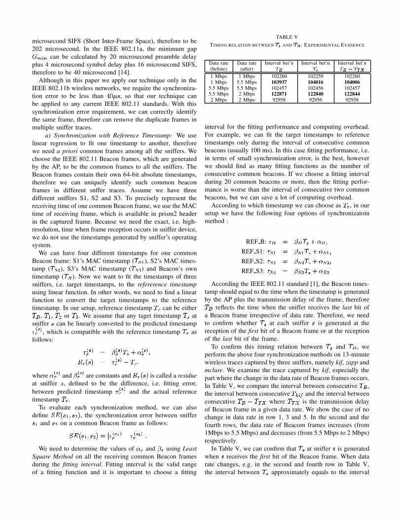
TABLE VTIMING RELATION BETWEEN M�N AND M!O : EXPERIMENTAL EVIDENCE
Data rate Data rate Interval bet’n Interval bet’n Interval bet’n(before) (after) MPO M�N M!ORQ�M�S!T1 Mbps 1 Mbps 102260 102259 1022601 Mbps 5.5 Mbps 103937 104016 104006
5.5 Mbps 5.5 Mbps 102457 102456 1024575.5 Mbps 2 Mbps 122871 122840 1228442 Mbps 2 Mbps 92958 92956 92958
interval for the fitting performance and computing overhead.For example, we can fit the target timestamps to referencetimestamps only during the interval of consecutive commonbeacons (usually 100 ms). In this case fitting performance, i.e.in terms of small synchronization error, is the best, howeverwe should find as many fitting functions as the number ofconsecutive common beacons. If we choose a fitting intervalduring 20 common beacons or more, then the fitting perfor-mance is worse than the interval of consecutive two commonbeacons, but we can save a lot of computing overhead.
According to which timestamp we can choose as � $ , in oursetup we have the following four options of synchronizatoinmethod :
REF B: & " , - "U� % .10V" 2REF S1: & � � , - � � � % .W0L� � 2REF S2: & �!� , - �!�X� % .W0L�!� 2REF S3: & �! , - �! X� % .W0L�!
According the IEEE 802.11 standard [1], the Beacon times-tamp should equal to the time when the timestamp is generatedby the AP plus the transmission delay of the frame, therefore�#" reflects the time when the sniffer receives the last bit ofa Beacon frame irrespective of data rate. Therefore, we needto confirm whether � % at each sniffer � is generated at thereception of the first bit of a Beacon frame or at the receptionof the last bit of the frame.
To confirm this timing relation between � % and �#" , weperform the above four synchronization methods on 13-minutewireless traces captured by three sniffers, namely kif, zapp andmclure. We examine the trace captured by kif, especially thepart where the change in the data rate of Beacon frames occurs.In Table V, we compare the interval between consecutive �V" ,the interval between consecutive �VY ��Z and the interval betweenconsecutive � " 9 �#[]\ where �#[^\ is the transmission delayof Beacon frame in a given data rate. We show the case of nochange in data rate in row 1, 3 and 5. In the second and thefourth rows, the data rate of Beacom frames increases (from1Mbps to 5.5 Mbps) and decreases (from 5.5 Mbps to 2 Mbps)respectively.
In Table V, we can confirm that �V% at sniffer � is generatedwhen � receives the first bit of the Beacon frame. When datarate changes, e.g. in the second and fourth row in Table V,the interval between � % approximately equals to the interval

-250
-200
-150
-100
-50
0
50
1 2 3 4 5 6 7 8 9 10 11 12
Fitti
ng E
rror
(use
c)
Elapsed Time (minutes)
Beacon Time vs. Fitting error (REF_B)
mclurekif
zapp
Fig. 32. Residue (fitting error) _LOA`�acbFdcd�e , _VOA`�f8gihje and _/OA`k�lGmKnjoqpIein REF B method with 5658 common beacon interval. Zapp, kif and mclureindicates the three wireless sniffers.
-250
-200
-150
-100
-50
0
50
1 2 3 4 5 6 7 8 9 10 11 12
Fitti
ng E
rror
(use
c)
Elapsed Time (minutes)
Beacon Time vs. Fitting error (REF_M)
mclurekif
zapp
Fig. 33. Residue (fitting error) _Lrs`tacbGdXd�e , _Vru`�f8gihje and _/r?`k�lGmKnjoqpIein REF M (REF Mclure) method with 5658 common beacon interval.
between ��" 9 � [^\ , where � [^\ is the transmission delay ofBeacon frame in a given data rate. We can also observe thatwhen data rate increases, the interval between ��" ’s becomesless than the interval between � % ’s (in the second row inTable V) and when data rate decreases, the interval between� " ’s becomes greater than that between �V% ’s (in the fourthrow). Therefore we can confirm that � " equals to the time ofsniffer receiving the last bit of the Beacon frame transmittedby the AP.
Based on this timing relation between � % and �#" , we cannotice the problem of REF B method, that is, whenever thedata rate of Beacon frames changes, the AP resets ��" . Putin other way, whenever the data rate changes, the clock �V"becomes a new clock, therefore is very unstable in terms ofthe usage of reference time.
To identify this problem emperically, we examine theresidue
4 " , i.e. difference between predicted timestamp ofeach sniffer and � " , in Figure 32. We observe that manydiscontinuities occur in Figure 32 and the times of thosediscontinuites coincide with when data rate of Beacon frames
changes due to variable channel condition. On the other hand,in REF Mclure (REF M, in short) method in Figure 33, suchdiscontinuities are not noticed.
Therefore, to correctly convert the sniffer timestamp to Bea-con timestamp, we need to use the adjusted time, ��" 9 � [^\ ,instead of using �#" , so that the Beacon timestamp can bestable even when the data rate changes. We need to use thefollowing equation instead of REF B equation:
ADJ B: &Xv , & " 9 � [^\ ,w- v � % .10 v JIn the followings, we compare the results of the above four
synchronization methods applied on the real data, ADJ B,REF M, REF K (REF kif) and REF Z (REF zapp) in termsof synchronization error =�>?5;�j� 2 � � 7 . We also compare vari-ous fitting intervals (e.g. interval of two common Beacons,200 common Beacons, 1000 common Beacons and more) todetermine which can best satisfy our requirement of synchro-nization error.
b) Performance of Time Synchronization Methods: Onthree 13-minute traces captured by three sniffers, mclure, kifand zapp, we perform the four synchronization methods toobtain the synchronization error =�>?56�j� 2 � � 7 among the threesniffers.
We find that all the three sniffers observe 5658 commonBeacons from an AP (say, AP1) during 13 minutes. Wegenerate the synchronization parameters 0 ' %*)$ and - ' %*)$ for eachsniffer MAC timestamp � % for each synchronization interval.For example, if we apply ADJ B method with the intervalof 1000 common Beacons to the 13-minute trace, then wehave 6 5 ,yx;zj{�z�|!}�~ �����@�@7 intervals, each of which has distinctfitting equation. For the trace of mclure, we calculate 6 pairsof 0 '
���6��� $��*)" and - '���6�� $I�*)" for each interval from � ���6��� $��
and �#" 9 � [^\ of the common Beacon frames. In the sameway, we also calculate those parameters for the traces of kifand zapp. We use Matlab function robustfit() to calculate thesynchronization parameters 0 and - .
Once we have the synchronization parameters for eachsniffer for each synchronization interval, we apply thoseparameters to the sample data to obtain =�>R5;� 2F� 7 , =�>?5 ��2I� 7and =�>?5 ��2 ��7 respectively. The sample data consists of5681 common Beacons, which however are from another AP(say, AP2). Therefore, we can compare the synchronizationperformance on different sample data from the 5658 commonBeacons we use for generating synchronization parameters.
In Table VI, we present the maximum values of =�>?56� � 2 �B�87 ,i.e. the maximum difference between predicted timestamps oftwo sniffer � � and �8� , of different synchronization methodswith various synchronization intervals (10000, 1000, 200 andtwo in our experiment). We can observe that as the inter-val decreases, the synchronization performance increases, i.e.maximum =�> decreases. The method ADJ B with the intervalof 5658 performs worse than other methods. However, withthe interval of 1000 or shorter, all the four methods show goodperformances, i.e. they satisfy the error requirement: less than40 microseconds.
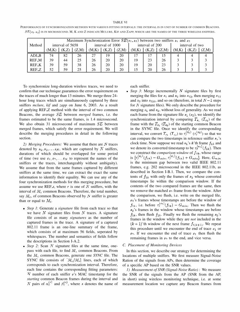
TABLE VIPERFORMANCE OF SYNCHORONIZATION METHODS WITH VARIOUS FITTING INTERVALS: THE INTERVAL IS IN UNIT OF NUMBER OF COMMON BEACONS.��� `��q�I�6���Ie IS IN MICROSECOND. M, K AND Z INDICATE MCLURE, KIF AND ZAPP, WHICH ARE THE NAMES OF THE THREE WIRELESS SNIFFERS.
Maximum Synchronization Error =A>?5;� � 2 �B�87 between two sniffers � � and �8�Method interval of 5658 interval of 1000 interval of 200 interval of two
(M,K) (K,Z) (Z,M) (M,K) (K,Z) (Z,M) (M,K) (K,Z) (Z,M) (M,K) (K,Z) (Z,M)ADJ B 74 82 26 27 19 20 17 17 15 4 4 4REF M 39 44 25 26 20 20 19 23 26 3 3 3REF K 39 59 38 26 20 20 19 20 23 3 3 3REF Z 52 59 25 26 20 20 15 20 26 3 3 3
To synchoronize long-duration wireless traces, we need toconfirm that our technique guarantees the error requirement onthe traces of much longer than 13 minutes. We merge three 24-hour long traces which are simultaneously captured by threesniffers mclure, kif and zapp on June 6, 2003. As a resultof applying REF Z method with the interval of two commonBeacons, the average =�> between merged frames, i.e. theframes estimated to be the same frames, is 1.4 microsecond.We also obtain 31 microsecond of maximum =�> betweenmerged frames, which satisfy the error requirement. We willdescribe the merging procedures in detail in the followingsection.
2) Merging Procedures: We assume that there are � tracesdenoted by �@� 2 � � 2BJXJXJ �B� , which are captured by � sniffers,durations of which should be overlapped for some periodof time (we use �j� 2 � � 2XJBJXJ �8� to represent the names of thesniffers or the traces, interchangeably without ambiguity).We assume that from the same frames captured by differentsniffers at the same time, we can extract the exact the sameinformation to identify their equality. We can use any of thefour synchronization methods for this merging procedure, butassume we use REF r, where � is one of � sniffers, with theinterval of � � common Beacons. Therefore, the total number,say � � , of common Beacons observed by � sniffer is greaterthan or equal to � � .� Step 1: Generate a signature file from each trace so that
we have � signature files from � traces. A signaturefile consists of as many signatures as the number ofcaptured frames in the trace. A signature of a captured802.11 frame is an one-line summary of the frame,which consists of at maximum 56 fields, seperated bywhitespaces. The number and semantics of fields followthe descriptions in Section I-A.2.� Step 2: Scan � signature files at the same time, one-pass with each file, to find � � common Beacons. Fromthe � � common Beacons, generate one SYNC file. TheSYNC file consists of x � � } � � � lines, each of whichcorresponds to each synchronization interval. Therefore,each line contains the corresponding fitting parameters:� number of each sniffer � ’s MAC timestamp for thestarting common Beacon frames during the interval and� pairs of 0 ' %*)$ and - ' %*)$ , where � denotes the name of
each sniffer.� Step 3: Merge incrementally � signature files by firstmerging the files for �j� and � � into �@� � , then merging �@� �and � into �@� �� , and so on (therefore, in total � 9 ~ stepsfor � signature files). We only describe the procedure formerging �j� and � � , without loss of generality. As we readeach frame from the signature file � � ( �8� ), we identify thesynchronization interval by comparing � % E ( � % H ) of theframe with the � % E ( � % H ) of the starting common Beaconin the SYNC file. Once we identify the correspondinginterval, we convert � % E ( � % H ) to & ' % E )$ ( & ' % H )$ ) so that wecan compare the two timestamps in reference sniffer � $ ’sclock time. Now suppose we read � � ’s � ’th frame � �FY andwe denote its converted timestamp to be & ' % E )$ 5;� �FY 7 . Thenwe construct the comparison window of �P�GY , whose rangeis � &(' %GEF)$ 5;���FYj7 9 � ���� 2 &(' %FE+)$ 56���GY�7L. � ����P� . Here,
� ���is the minimum gap between two valid IEEE 802.11frames, e.g. 202 microsecond in the IEEE 802.11b, asdescribed in Section I-B.1. Then, we compare the con-tents of ���FY with only the frames of � � whose convertedtimestamps lie within the comparison window. If thecontents of the two compared frames are the same, thenwe remove the matched �<� frame from the window. Afterthe comparison, we flush, i.e. write on the merged file,�8� ’s frames whose timestamps are before the window of� �GY , i.e. before & ' % E )$ 56� �FY 7 9 ������ . Then we flush the�8� ’s frames in the window whose timestamps are before� �GY , then flush � �GY . Finally we flush the remaining �<� ’sframes in the window while they are not included in the56��. ~ 7 ’th window of the next frame � � ' Yc�V�+) . We repeatthis procedure until we encounter the end of trace ��� or� � . If we encounter the end of trace �j� then flush theremaining frames in � � to the end, and vice versa.
C. Placement of Monitoring Devices
In this section, we describe our strategy for determining thelocations of multiple sniffers. We first measure Signal-NoiseRation of the signals from APs, then determine the coverageof a specific AP based on the SNR values.
1) Measurement of SNR (Signal-Noise Ratio) : We measurethe SNR of the signals from the AP (SNR from the AP,in short) using wireless monitoring technique, i.e. at somemeasurement location we capture any Beacon frames from

any AP observed there and examine the SNR values in Prism2header of the frames. In this way, we measure the SNRs at asmany locations as possible in the target area, then from themeasurement data we extract only the SNR from the target APto find the marginal SNR line, therefore we can determine thecoverage of the target AP, which is defined in the followingsection.
In Figure 34, we show the 15-dB marginal line, i.e. thecoverage of the AP, determined by applying the measurementtechnique. We give ESSID ”mindlab” to the AP, therefore wesetup an one AP wireless network. In other words, there are noother APs nearby with the same ESSID. At 132 measurementlocations in the fourth floor of A.V. Williams building, wecapture Beacon frames to obtain the average SNR for 30seconds (therefore about 300 Beacon frames per AP) at eachlocation. Then in off-line we extract the average SNRs fromthe target AP (with ESSID ”mindlab”) to obtain the SNRcontour lines of 40, 30, 20 and 15 dB, as shown in Figure 34.
We can measure the SNR from the target AP by associatingthe measurement device with the AP and examining the SNRonly from the AP. However, the problem of this method is thatit is difficult to force the measurement device to be associatedwith the AP, especially at the location far from the AP.
Applying wireless monitoring technique to measure theSNR gives another advantage that we can also obtain the SNRsfrom the other APs on same or other channels. Based on theSNRs from any observable APs at the location, we can obtainthe coverage of the APs in terms of the definition in previoussection in case there are other APs with the same ESSID as thetarget AP. We obtain the coverages of ESSID ”umd” APs inthe fourth floor of A.V. Williams building. In their coverages,the APs have greater SNR than from other APs, as shown inFigure 6.
2) Placement Strategies Based on SNR Measurement:Since in the infrastructure mode of the 802.11 protocol alltraffic goes through the AP, one may think that placing allsniffers near the AP should maximize the capture performance.However, our experiments showed that the capture perfor-mance of To-AP traffic is worse than that of the From-APtraffic, even for the sniffer T which was adjacent to the AP.This is due to the weak signal that reaches the sniffer fromthe clients compared to the strong signal that reaches the samesniffer from the AP. The AP can capture the weak signal dueto its better hardware and specialized processing (compared tothe sniffer configuration).
Therefore, for placing the wireless sniffers, we should onlyplace one sniffer adjacent to the AP to be responsible forcapturing the From-AP traffic and the traffic of clients nearthe AP. Other sniffers should be placed as close as possibleto the wireless clients.
If we assume that clients are going to be uniformly dis-tributed over the coverage area, this translates to placing thesniffers so that they cover as much as possible from the APcoverage area. Therefore, if we have � sniffers to place, wecan split the AP coverage area into � equal areas and placethe sniffers in the center of mass of these areas.
40
40
30
20
30 2015
AP
15224 feet
85.1 feet
UT
BG
V
Marginal line of coverage
SNR wallClientSniffer
AP
W
Fig. 34. SNR Contour Map for controlled experiment: SNR Contour linesfor 40,30,20 and 15 dB are obtained from SNR measurements. Based onthe contour map, we place the wireless stations at location G and B, placethe sniffers at location T, U, V and W. Several SNR Walls are detected byexamining the distances between adjacent contour lines.
We can refine this strategy by noting that, in an environmentwhere multiple APs are installed, the coverage area of anAP may be reduced to the Association Area of the AP. TheAssociation Area of an AP is the area at which a client willfavor this AP for association compared with other APs inthe area. Note that the Association area is a sub-area of thecoverage area and that most of the traffic an AP receives comesfrom the associated clients (i.e. from the Association Area).Therefore, we should use the association area of an AP ratherthan its coverage area. Fig. 6 shows the Association Areasfor different access points in the area of interest. The figurealso shows the difference between the coverage area and theassociation area for �� �
Another factor that needs to be taken into account is thesignal condition at the sniffer location. We define an SNR wallas an area where the SNR contour lines are close to eachother (Fig. 34). Our experiments (see Section II-D) shows thatplacing a sniffer near an SNR wall leads to worse captureperformance compared to placing the sniffer at other places.Therefore, SNR walls should be avoided.
APPENDIX IICONTROLLED EXPERIMENTS
To examine the effect of our wireless monitoring tech-niques, i.e. merging multiple sniffers and sniffer placement,we conduct controlled experiments using NetDyn, which wewill describe in the following section.
The purpose of this experiment is two-fold: first we examinethe effect of our monitoring techniques, i.e. multiple sniffermerging and placement, and second we quantitatively comparethe effect of our wireless monitoring technique with those ofthe other measurements, e.g. end-to-end measurement, SNMPand wired monitoring. The analysis in terms of the secondpurpose will be discussed in Section ??. We describe the setupof the controlled experiments in this section.

Source
NetDyn
SinkEcho
NetDynSrc TS
Source
NetDyn
Sink
NetDyn
NetDyn in two-way mode
NetDyn in one-way mode
Src SeqNum
Src TS Src SeqNumEcho TS Echo SeqNumSrc TS Src SeqNum
Echo TS Echo SeqNumSync TS
Src TS Src SeqNum Src TS Src SeqNum Sync TS
Fig. 35. Controlled Experiment using NetDyn: Source in a wireless stationsends 20000 UDP packets to wired Echo machine which sends them back toSink in the same wireless station.
A. Methodology
1) Environment : We perform our experiments in the fourthfloor of A.V. Williams building at University of Maryland(where Department of Computer Science is located). Thebuilding has 58 access points installed, which belong to threedifferent wireless networks. Each wireless network is identifiedwith its ESSID. The ESSIDs of the three networks are umd,cswireless and nist respectively. umd network consists of29 Cisco Aironet A-340 APs, and is the most widely usedwireless network in the university. cswireless (12 Lucent APs)and nist (17 Prism2-based APs) are built by individual researchresearch groups in the department.
2) NetDyn: End-to-end Traffic Measurement Tool: NetDyn[13] is an end-to-end traffic measurement tool, in whichUDP or TCP packets are actively injected to the network formeasuring available bandwidth of the network.
NetDyn consists of three different processes, Source, Echoand Sink and can operate in two modes, namely one-way ortwo-way. In two-way mode, Source process on sender machinegenerates a packet with timestamp and source packet numberand sends it to to Echo process on remote machine. As theEcho process receives the packet, it attaches its timestampand echo packet number to the packet, then send the packetback to Sink process, which is running also on sender ma-chine. After Source sends some number of packets and Sinkreceives them back, we can calculate the number of packetscorrectly transmitted between Source and Echo by comparingthe source packet number and echo packet number of thepackets successfully received by Sink process. We can alsocalculate RTT (Round Trip Time) between Source machineand Echo machine.
In one-way mode, Source process resides on the sendermachine, and Sink process is running on the receiver machine.As the name implies, the traffic is only from Source processto Sink process. In one-way mode, we can calculate only thenumber of packets successfully transmitted from Source toSink, but cannot obtain RTT between them.
This tool was originally designed for measuring the avail-
TABLE VIICONTROLLED EXPERIMENT SETUP: MODE INDICATES NETDYN MODE,EITHER ONE-WAY OR TWO-WAY.G DENOTES THE STATION AT LOCATION
G, B DENOTES THE STATION AT LOCATION B, S DENOTES THE NETDYN
SERVER, WIRED BEHIND THE AP.
Exp. # Mode Src. Dst. # Pkts Inter-Pkt TimeExp. 1 Two-way G S 20000 10 k��
Two-way B S 20000 10 k��Exp. 2 One-way B S 20000 5 k��
One-way S G 20000 5 k��Exp. 3 One-way S B 20000 5 k��
One-way G S 20000 5 k��
able bandwidth in wide-area network, we use it in this work forgenerating and measuring the traffic in wireless LAN. Fig. 2shows the setup for NetDyn running in two-way mode onwireless LAN. Source and Sink processes run on a wirelessstation (a mobile laptop) in our setup, while Echo process runson a server wired to Ethernet Local Area Network. By Source,Sink and Echo, we mean in this paper those processes or themachines where they run.
3) Setup for Wireless Network: Because we need morecontrolled environment to examine the effectiveness of ourtechnique quantitatively, we set up a separate wireless networkwith ESSID ”mindlab” in this experiment.
We have one Orinoco AP-1000 wireless access point withOrinoco Silver wireless card at the location AP in Figure 34.The AP is wired to the server machine = , on which werun NetDyn processes, Source, Sink and Echo. We have twowireless stations, namely
�and � at locations G and B in
Figure 34, on each of which NetDyn processes Source andSink run. Location G and B represents a Good location interms of signal condition and a Bad location respectively. Gis located at 40-dB line 12-feet apart from the AP and B ison the 15-dB marginal line of SNR from the AP. The twowireless stations are equipped with the same wireless card asthe AP.
4) Setup for Wireless Monitoring, Wired Monitoring andSNMP: We place the three sniffers at locations T, U and Vrespectively in Figure 34. Those sniffers run the same H/Wand S/W described in Section I-A. We merge the three traceswith REF V (V is also used for the name of the sniffer) withthe interval of two consecutive common Beacons from the AP.
To measure the wired traffic, we set up one wired snifferbetween the server = and the AP. The wired traffics betweenthe server = and the AP in both direction are captured onthe wired sniffer through the ”Century Tap”, a full-duplex10/100 Ethernet splitter [20]. We capture the wired trafficsusing Ethereal on the wired sniffer = .
On the wired sniffer, we also run a SNMP client, snmputil,which is written by Balachandran etal. for the previous re-search [2]. We make snmputil polling the AP every minute,similar to the setup in [2].

B. Generating Wireless Traffics
For generating traffic as realistic in actual wireless LANas possible, we run three different experiments, the setup ofwhich are summarized in Table VII. In Experiment 1 (Exp. 1,in short), we have two two-way NetDyn traffics between twowireless stations
�, � and wired server = . Wireless station�
( � ) runs Source and Sink processes, at the same time theserver = runs Echo.
�( � ) send 20000 packets of full UDP
payloads (1472 bytes) to = , with 10 ¡� inter-packet. In otherdirection, = sends back the packets to
�and � . Therefore in
Exp. 1, we have generated UDP traffic of roughly 4.7 Mbit persecond (aggregately in both directions) on wireless medium.
In Exp. 2, we instead have two one-way NetDyn trafficsbetween two wireless stations
�, � and wired server = .
Wireless station � runs Source process to send 20000 packetsof full UDP payloads (1472 bytes) with 5 ¢� to correspondingSink process on the server = At the same time in otherdirection, the Source process on the server = sends the sameamount of traffic to the Sink on another wireless statin
�.
Therefore in Exp. 2, we have also generated UDP traffic ofroughly 4.7 Mbit per second on wireless medium. Exp. 3 hasthe same setup as Exp. 2 except having the traffics in reversedirections.
Exp. 1 emulates the realistic situation that a STA in goodlocation in terms of signal condition and another STA in badlocation both try to communicate with the remote server(s).Exp. 2 (Exp. 3) is a scenario similar to the situation that onesender STA in bad (good) location and one receiver STA ingood (bad) location run at the same tme in the same wirelessLAN.
C. The Effect of Merging
We estimate the measurement loss improvement of mergingmultiple sniffers by conducting an controlled experiment.We can calculate the measurement loss by looking at MACsequence number field as shown in [11], but we find that thismethod is not accurate due to the misbehaviors of variouswireless cards and the AP. We notice that there exist some (inone trace 41 frames out of 125057) out-of-sequence framesin their MAC sequence number. By out-of-sequence frames,we mean one frame’s MAC sequence number is less thanthe previous frame’s MAC sequence number even thoughthe interval between two frames is not long enough for thetwo numbers to wrap around. The range of the IEEE 802.11MAC sequence number is � � 2 �!��£ z � , therefore for two sequencenumbers of consecutive frames to wrap around, the intervalshould be greater than
�¤�����¥ ����£ { .Others reported that such out-of-sequence MAC sequence
number can be generated by some wireless stations formalicious attack [12]. Therefore, for estimating the exactmeasurement loss, we need to use reliable sequence numbersgenerated by the applications. This is the reason why weconduct two-way UDP packet exchange experiments usingan end-to-end traffic measurement tool, called NetDyn [13],described in Section II-A.2.
TABLE IXTHE EFFECT OF PLACEMENT (WITH THREE SNIFFERS AT LOCATIONS T, U
AND V): THE NUMBER OF NETDYN PACKETS CAPTURED ON EACH
SNIFFER IS PRESENTED. THE COLUMN Dist. SHOWS THE NUMBER OF
DISTINCT PACKETS, THE COLUMN All ALSO INCLUDES THE NUMBER OF
RETRANSMISSIONS. THE NUMBERS ARE NORMALIZED WITH RESPECT TO
THE NUMBER CAPTURED BY SNIFFER AT T.
Sniffer at T Sniffer at U Sniffer at VTraffic Dist. All Dist. All Dist. All
Exp.1 (G ¦ S) 100 100 96.0 95.8 95.2 95.1Exp.1 (G § S) 100 100 98.9 98.8 96.8 96.7Exp.1 (B ¦ S) 100 100 143.3 171.5 143.5 172.5Exp.1 (B § S) 100 100 99.8 129.9 100.2 128.0Exp.2 (B ¦ S) 100 100 185.7 217.5 186.6 219.7Exp.2 (G § S) 100 100 99.4 99.4 98.7 98.6Exp.3 (G ¦ S) 100 100 89.9 89.8 89.0 89.0Exp.3 (B § S) 100 100 100.5 101.3 99.9 98.3Total (G ¨ S) 100 100 96.4 96.3 95.3 95.2Total (B ¨ S) 100 100 126.5 145.2 126.7 144.3
Total (From-AP) 100 100 99.6 107.1 98.8 105.2Total (To-AP) 100 100 121.2 134.4 120.9 134.6
Table VIII shows the effect of using the merged sniffers’traces. We show the result of Exp. 1 only, but in other experi-ments we have similar observations. We can see from the tablethat increasing the number of merged sniffers’ traces from oneto two to three increases the percentage of captured framessignificantly from 73.25% to 84.47% to 99.34% respectivelyfor the To-AP traffic. Notice also that the effect of mergingis more significant in the case of To-AP traffic while a singlesniffer near the AP (sniffer T) can almost capture all the From-AP traffic (improvement from T only to T+U+V is 0.7%).Using the merged three-sniffers ’ trace, wireless monitoringcan capture more than 99.34% of the wireless traffic.
D. The Effect of Placement
To examine the effect of our placement technique describedin Section I-C, we place three sniffers according to thetechnique during the controlled experiment in Table VII.
In Figure 34, for capturing the traffic between the AP andthe STA at location
�(STA
�, in short), we place one sniffer
at the middle point between them, i.e. at location T. As anotherSTA is at location � (STA � , in short), which is on themarginal line of the AP coverage, we place the other twosniffers around the middlie point between the STA and theAP.
For the placement of the other two sniffers we choose threepoints U, V and W. U is located exactly on 30-dB line, V iscloser to the client STA � than 30-dB line. W is more offthan 30-dB line, even closer to STA � than V. Noticeably, thelocation W is close to one of the SNR Walls, which is detectedby the SNR contour lines in Figure 34.
Due to only three sniffers available at the same time, werun the set of experiments in Table VII two times. In the firstround, we place the sniffers at U and V and run Exp 1., Exp.2and Exp.3. In next round of Exp. 1-3, we place the sniffers atU and W and conduct the same experiments.

TABLE VIIIINCREASING CAPTURED FRAMES BY MERGING MULTIPLE SNIFFERS: MERGING TWO OR THREE SNIFFERS AMONG T, U AND V SIGNIFICANTLY
INCREASES THE NUMBER OF OBSERVED FRAMES. (WE SHOW THE RESULT OF EXP. 1 ONLY)
To-AP Wireless TrafficNetDyn T U V T+U T+V U+V T+U+V
Good 19905 76.76% 69.00% 68.34% 76.83% 70.00 % 76.84% 98.61%Bad 18490 69.48% 99.58% 99.73% 99.05% 100.0 5% 99.97% 100.13%Total 38395 73.25% 83.73% 83.46% 87.54% 84.47% 87.98% 99.3 4%
From-AP Wireless TrafficGood 19247 98.41% 97.31% 95.24% 99.37% 98.06% 99.32% 99.38%Bad 17858 102.04% 101.85% 102.2% 102.56% 102.43% 102.52% 102.56%Total 37105 100.15% 99.5% 98.59% 100.91% 100.16% 100.86% 100.91%
TABLE XTHE EFFECT OF PLACEMENT (WITH THREE SNIFFERS AT LOCATIONS T, U
AND W)
Sniffer at T Sniffer at U Sniffer at WTraffic Dist. All Dist. All Dist. All
Exp.1 (G ¦ S) 100 100 87.3 87.2 84.5 84.4Exp.1 (G § S) 100 100 96.5 96.7 87.6 87.7Exp.1 (B ¦ S) 100 100 138.7 171.0 136.3 169.2Exp.1 (B § S) 100 100 100.2 100.2 98.3 93.2Exp.2 (B ¦ S) 100 100 125.7 146.7 125.4 147.7Exp.2 (G § S) 100 100 93.4 93.3 72.9 72.8Exp.3 (G ¦ S) 100 100 80.4 80.3 78.4 78.4Exp.3 (B § S) 100 100 100.0 96.7 97.5 88.1Total (G ¨ S) 100 100 89.5 89.5 81.2 81.1Total (B ¨ S) 100 100 115.1 122.5 113.4 117.8
Total (From-AP) 100 100 97.4 97.1 89.0 86.4Total (To-AP) 100 100 105.4 117.5 103.5 116.0
In Table IX, we show the number of NetDyn packetscaptured by the three sniffers (denoted by sniffer T, U andV respectively) in the first round of experiments. We observethat in both distinct number and all number (retransmissionsincluded), the sniffer T performs best for the traffic betweenSTA
�and the server = (therefore between
�and the AP).
This is due to the fact that sniffer at T is the closest to boththe AP and STA
�. Likewise, for
�- = traffic, the sniffer
U performs better than the sniffer V due to its physicallycloseness to
�.
For the traffic between STA � and the server = , thereforethe AP, the sniffer U captures more �ª©«= than the snifferV, while the sniffer V captures more �¬®= than the snifferU. This also agrees with their relative closeness to = and �respectively.
Table X shows the number of captured frames by thesniffers when we place them at T, U and W. Even thoughthe location W is much closer to STA � than the location U,the performance of the sniffer W for �D¬¯= is no better thanthe sniffer U, even slightly worse. We infer that the SNR Wallright next to the location W affects the performance of thesniffer W. For the traffics other than �D¬°= traffic, the snifferW shows worse performance than the sniffer V, which agrees
with its physical remoteness from the AP.From Table VIII, Table IX and Table X we conclude as
follows:� The location of the sniffer is one of the most influencingfactors in sniffing performance in terms of number ofcaptured packets.� Different sniffers have different viewpoints of the wire-less medium.� The absolute physical location of the client or the snifferdoes not affect the ability of a particular sniffer to capturedata from a particular wireless client. Rather, the relativeposition between the wireless client and the sniffer is thefactor that affects the ability of a sniffer to capture thedata from that client.For example, for the traffic originating from STA � ,sniffers U and V capture more traffic than sniffer T. Thereason for that is as the distance from the sniffer to thewireless client increases, the signal strength decays andthe SNR decreases leading to worse signal conditionsand decreased sniffing performance. Sniffers U and V arecloser to STA � than sniffer T.� For From-AP traffics, showed in Total (From-AP) row, thesniffer T outperforms other sniffers in Distinct numbers,but with retransmissions included, other sniffers canperform better. This means that the sniffer dedicated tothe AP reflects more the AP-oriented view, while othersshow more the STA-oriented or medium-oriented view.� SNR Walls affect the sniffer performance, therefore weshould avoid placing the sniffer near the SNR Walls evenif the place agrees our placement strategy.
APPENDIX IIICOMPARISON WITH END-TO-END MEASUREMENT, SNMP
AND WIRED MONITORING
In the controlled experiment in the previous section, wehave also measured the traffic with other methods, e.g. wiredmonitoring and SNMP. In this section, we quantitatively com-pare the results obtained from those methods with our wirelessmonitoring technique. We apply the techniques of multiplesniffer merging to obtain the statistics on wireless traffics withthe experimental setup in Table VII. This comparison can

provide the pros and cons of our wireless monitoring techniquecompared to the other methods, prevalently used for wirelessLAN measurement.
A. Comparison Results
As Table XI shows, we have seven statistics from variousmethods, e.g. end-to-end, SNMP based on MIB-I, SNMPbased on MIB-II, wired monitoring and wireless monitoring.We also show in TableXII, XIII, XIV and XV, the statisticsof the same experiments, but presenting per-experiment, per-station details.
We compare those methods with respect to the six values,# Packets, # ReTX (Retransmissions), # Errors in inbound(STA ¬ server = ) and outbound ( =±¬ STA) traffics.
To compare the various values from different measurementtechniques, we should note that each statistics has differentmeaning. Therefore those statistics cannot be blindly com-pared value by value without careful consideration of thesemantics. For example, # Errors in end-to-end measurementindicates # Frames not received by the destination application,while # Errors in SNMP measurement is defined to # Framesnot sent (or received) by the AP. Therefore, we first explainin detail the semantics and the result of each statistics, thencompare each statistics with others.� End-to-end measurement using NetDyn (Table XI-1): we
obtain # NetDyn UDP packets correctly received by thedestination by examining packet numbers generated byNetDyn processes. We define # Errors to be the number ofNetDyn packets which are sent by NetDyn Source processbut NOT received by NetDyn Sink process. Thereforethis number can include the number of errors occuringat TX/RX buffers on Source or Sink machines, the errorson wired medium, the errors at the AP, and the errors onwireless medium. With the end-to-end trace at each STAand the server = , we can break down the statistics into thetraffic from/to Good STA (at location
�) and the traffic
from/to Bad STA (at location � ). In total, inbound trafficis more successfully transmitted than outbound traffic. Inonly inbound traffic, the traffic from Good STA (
�, in
short) experiences more errors than Bad STA ( � ). Thereason is that the signal condition during Exp. 3 becomesmuch worse than during Exp. 2 (refer to Table VII forexperimental setup). Therfore, during Exp. 3 the one-wayexperiment
� ¬²= experiences severe losses, while theone-way experiment �³¬ = in Exp. 2 does not. Onthe other hand, in outbound traffics, the traffics to
�has much more successful transmissions than those to� . This is partly due to the same reason describe abovethat the traffic =´¬µ� in Exp. 3 experiences worse signalcondition. The another reason is due to the ”bad” locationof STA � .� SNMP measurement with MIB-I (Table XI-2): we retainthe SNMP log of up-to-date aggregate statistics at the APin one minute interval. From this log, we obtain the differ-ence between the statistics at the start of the experimentand the statistics at the end of the experiment. Because
the resolution of measurement time is one minute, thenumbers presented can have maximum error up to thenumbers of two-minute intervals (during about 30 minuteexperiments). According to the definitions in [16] and [2],we can define the statistics as follows: # Inbound Packetsindicates # unicast frames successfully delivered to ahigher-layer protocol (e.g. IP). # Inbound Errors indicates# errors preventing frames from being deliverable to ahigher-layer protocol. # Outbound Packets is defined tobe the total number of packets that higher-level protocolsrequest to be transmitted to a subnetwork-unicast address.Note that # Outbound Packets include those frames thatare discarded or not sent due to the errors. We calculate# Outbound ReTX using the technique in [2] by takingthe difference between the number of inbound packetsat wired interface and # Outbound Packets. # OutboundErrors is defined to be the number of outbound framesthat could not be transmitted because of errors. Notethat # Outbound Errors contains the number of errorsin broadcast packets, e.g. Beacons. Intuitively, # InboundPackets is the number of frames the AP receives success-fully, # Outbound Packets is the number of the AP sends,and both are the exact statistics the AP can measure.However, # Errors is the aggregate number of errors inboth unicast and broadcast packets, therefore the exacterror statistics for only unicast packets are not availablewith MIB-I. In sub-table 2, we notice 8.2% of inbounderrors and 3.8% of outbound errors, which are both higherthan 2.41% error rate, which are obtained with the samemethod in public conference [2]. In their setup they havefour different APs, but within the similar area we haveonly one AP, therefore worse signal conditions of oursetup result in higher error rate. In their results, thenumber of (outbound) retransmissions is less than thenumber of errors, and they explain the mismatch withthe errors in Beacon frames. In contrast, even thoughthe same method is applied in our results, # OutboundReTX is about 5 times more than # Outbound Errors.This implies that in our controlled experiment the locationof STA � incurs severe retransmissions between � andthe AP. # ReTX is the value estimated using the methodin [2]. We will show more accurate statistics on errorsand retransmission using MIB-II in the followings, thencompare the MIB-II measurement result with the resultof our wireless monitoring technique.� SNMP measurement with MIB-II (Table XI-3): we can ob-tain more accurate statististics with MIB-II [17], [18]. Es-pecially we can have accurate statistics on errors and out-bound retransmissions for unicast packets. MIB-II trans-mission group defines various objects for dot3 type inter-face, i.e. ethernet-like interface type [18]. For outboundretransmission, the variables SingleCollisionFrames, Mul-tipleCollisionFrames and ExcessiveCollisionFrames aredefined. SingleCollisionFrames and MultipleCollision-Frames indicate the number of frames retransmitted onceand two times respectively to be finally successfully

TABLE XIQUANTITATIVE COMPARISON BETWEEN END-TO-END MEASUREMENT USING NETDYN, SNMP, WIRED MONITORING AND WIRELESS MONITORING
Inbound (To-AP) Wireless Traffic Outbound (From-AP) Wireless TrafficStatistics # Packets # ReTX (%) # Errors (%) # Packets # ReTX (%) # Errors (%)
1. NetDyn End-to-End Measurement# Packets: # DISTINCT NetDyn UDP packets correctly received by the destination,# Errors: # DISTINCT NetDyn UDP packets NOT received by the destination.
1. Total 75310 - 4690 (5.9%) 69403 - 9102 (11.4%)(Good STA) 36831 - 3169 (7.9%) 39247 - 658 (1.6%)(Bad STA) 38479 - 1521 (3.8%) 30156 - 8444 (21.1%)
2. SNMP Measurement with MIB-I in [2]# Inbound Packets: # frames received by AP without errors/discards.# Inbound Errors: # errors preventing frames from being deliverable to a higher-layer protocol.# Outbound Packets: # frames TXed by AP, including errors/discards.# Outbound ReTX: the difference between # inbound packets at wired interface and # outbound packets at w ireless interface.# Outbound Errors: # errors at AP, including the errors in broadcast packets.
2. Total 75494 - 6727 (8.2%) 71959 14536 (16.8%) 2740 (3.8%)3. SNMP Measurement with MIB-II# Packets: defined same as MIB-I.# Inbound Errors: sum of variables FCSErrors and InternalMacReceiveErrors.# Outbound ReTX: sum of variables SingleCollisionFrames, MultipleCollisionFrames and ExcessiveCollisions.# Outbound Errors: sum of variables ExcessiveCollisions, LateCollisions, CarrierSenseErrors and InternalMacTransmitErrors.
3-1. Total 75494 - 6726 (8.2%) 71959 10793 (15.0%) 2944 (3.8%)# Packets: # successfully RXed/TXed frames.# Outbound ReTX: # successfully ReTXed frames.
3-2. Total 75494 - - 69015 7849 (11.4%) -4. Wired Monitoring# Packets: # DISTINCT frames found in the wired traces.
4. Total 75312 - - 78335 - -(Good STA) 36832 - - 39908 - -(Bad STA) 38480 - - 38427 - -
5. Wireless Monitoring checked with the IEEE 802.11 ACK# Packets: # DISTINCT observed data frames with the corresponding 802.11 ACK observed,# Errors: # DISTINCT observed data frames without 802.11 ACK observed,
(32.4%)(34.2%)5. Total 53475 - 19956 (27.2%) 50183 - 21198 (29.7%)
(Good STA) 24421 - 10512 (31.8%) 28958 - 10150 (32.4% )(Bad STA) 29054 - 9444 (24.5%) 21225 - 11048 (34.2%)
6. Wireless Monitoring checked with NetDyn results# Packets: # DISTINCT observed data frames found to be in NetDyn traces,# Errors: # DISTINCT data frames NOT observed but found to be in NetDyn traces.
6. Total 73364 - 1940 (2.6%) 69236 - 167 (0.2%)(Good STA) 34912 - 1913 (5.2%) 39092 - 155 (0.4%)(Bad STA) 38452 - 27 (0.1%) 30144 - 12 (0.0%)
7. Wireless Monitoring checked with Retransmissions
)# Packets: # DISTINCT observed data frames,# Errors: # DISTINCT observed retransmissions, i.e. frames with 802.11 RETRY field set.
7. Total 73431 11815 (16.1%) - 71381 9980 (14.0%) -(Good STA) 34933 1170 (3.3%) - 39108 394 (1.0%) -(Bad STA) 38498 10645 (27.7%) - 32273 9586 (29.7%) -

TABLE XIINETDYN RESULTS, PER EXP, PER STA: ONLY DISTINCT FRAMES ARE COUNTED.
To-AP From-APTraffic # Packets # ReTX # Err. (%) # Packets # ReTX # Err. (%)
Exp.1 (G ¬ S) 19905 - 95 (0.5%) - - -Exp.1 (G © S) - - - 19247 - 658 (3.3%)Exp.1 (B ¬ S) 18490 - 1510 (7.6%) - - -Exp.1 (B © S) - - - 17858 - 632 (3.4%)Exp.2 (B ¬ S) 19989 - 11 (0.1%) - - -Exp.2 (G © S) - - - 20000 - 0 (0.0%)Exp.3 (G ¬ S) 16926 - 3074 (18.5%) - - -Exp.3 (B © S) - - - 12298 - 7812 (39.1%)Total (G ¶ S) 36831 - 3169 (7.9%) 39247 - 658 (1.6%)Total (B ¶ S) 38479 - 1521 (3.8%) 30156 - 8444 (21.1%)
Total 75310 - 4690 (5.9%) 69403 - 9102 (11.4%)
TABLE XIIIWIRELESS MONITORING CHECKED WITH ACK, PER EXP, PER STA: ONLY DISTINCT FRAMES ARE COUNTED.
To-AP From-APTraffic # Packets # ReTX # Err. (%) # Packets # ReTX # Err. (%)
Exp.1 (G ¬ S) 13905 - 5725 (29.2%) - - -Exp.1 (G © S) - - - 13522 - 5607 (29.3%)Exp.1 (B ¬ S) 13437 - 5078 (27.4%) - - -Exp.1 (B © S) - - - 12741 - 5575 (30.4%)Exp.2 (B ¬ S) 15617 - 4366 (21.8%) - - -Exp.2 (G © S) - - - 15436 - 4543 (22.7%)Exp.3 (G ¬ S) 10516 - 4787 (31.3%) - - -Exp.3 (B © S) - - - 8484 - 5473 (39.2%)Total (G ¶ S) 24421 - 10512 (31.8%) 28958 - 10150 (32.4%)Total (B ¶ S) 29054 - 9444 (24.5%) 21225 - 11048 (34.2%)
Total 53475 - 19956 (27.2%) 50183 - 21198 (29.7%)
TABLE XIVWIRELESS MONITORING CHECKED WITH NETDYN, PER EXP, PER STA: ONLY DISTINCT FRAMES ARE COUNTED.
To-AP From-APTraffic # Packets # ReTX # Err. (%) # Packets # ReTX # Err. (%)
Exp.1 (G ¬ S) 19619 - 289 (1.5%) - - -Exp.1 (G © S) - - - 19113 - 134 (0.7%)Exp.1 (B ¬ S) 18480 - 10 (0.0%) - - -Exp.1 (B © S) - - - 17854 - 4 (0.0%)Exp.2 (B ¬ S) 19972 - 17 (0.0%) - - -Exp.2 (G © S) - - - 19979 - 21 (0.1%)Exp.3 (G ¬ S) 15302 - 1624 (9.6%) - - -Exp.3 (B © S) - - - 12290 - 8 (0.0%)Total (G ¶ S) 34912 - 1913 (5.2%) 39092 - 155 (0.4%)Total (B ¶ S) 38452 - 27 (0.1%) 30144 - 12 (0.0%)
Total 73364 - 1940 (2.6%) 69236 - 167 (0.2%)

TABLE XVWIRELESS MONITORING CHECKED WITH RETRANSMISSIONS, PER EXP, PER STA: ONLY DISTINCT FRAMES ARE COUNTED.
To-AP From-APTraffic # Packets # ReTX (%) # Err. # Packets # ReTX (%) # Err.
Exp.1 (G ¬ S) 19630 576 (2.9%) - - - -Exp.1 (G © S) - - - 19129 386 (2.0%) -Exp.1 (B ¬ S) 18515 5121 (27.7%) - - - -Exp.1 (B © S) - - - 18316 4181 (22.8%) -Exp.2 (B ¬ S) 19983 5522 (27.6%) - - - -Exp.2 (G © S) - - - 19979 8 (0.0%) -Exp.3 (G ¬ S) 15303 594 (3.9%) - - - -Exp.3 (B © S) - - - 13957 5405 (38.7%) -Total (G ¶ S) 34933 1170 (3.3%) - 39108 394 (1.0%) -Total (B ¶ S) 38498 10645 (27.7%) - 32273 9586 (29.7%) -
Total 73431 11815 (16.1%) - 71381 9980 (14.0%) -
transmitted. ExcessiveCollisionFrames is an error statis-tics for the number of frames retransmitted but failingto be transmitted. Other error statistics for outboundinterface include CarrierSenseErrors i.e. # times that thecarrier sense condition was lost, LateCollisions i.e. #times that collision is detected after 512 bit is transmittedand InternalMacTransmitErrors for other kinds of errors.The objects for inbound errors include FCSErrors i.e.the number of errors in Frame Check Sequence, andInternalMacReceiveErrors for other kinds of errors. Withthose variables, in sub-table 3-1 in Table XI, we haveexact # Inbound Errors, # Outbound ReTX and # Out-bound Errors. We can also calculate the statistics for onlyRX/TX successes by subtracting # Errors from # Packets,as shown in sub-table 3-2. Note that # Inbound Packetsin sub-table 3-1 does not include # Errors, therefore hasthe same value in both (3.1) and (3.2).� Wired monitoring (Table XI-4): from the wired tracescaptured between the server = and the AP, we obtainDISTINCT number of packets to/from each STA. Mostof the frames captured by wired sniffer are NetDynpackets (75333 out of 75340 for inbound traffic, 78348out of 78355 for outbound traffic). Most of the framescaptured are NOT duplicated. Only 28 (20) packets areduplicated for inbound (outbound) traffic. With sourceand destination IP addresses available in the traces, wecan break down the statistics per STA. The numberof outbound packets captured by wired monitoring, i.e.78348, is much greater than actual end-to-end successfultransmissions, i.e. 69403, by roughly 10000 packets. Thisshows that as the signal condition become worse, theaccuracy of wired monitoring is severely reduced.� Wireless monitoring checked with the IEEE 802.11 ACK(Table XI-5): We calculate the statistics on the mergedtrace from three different wireless sniffers T, U andV in Figure 34. One way to obtain the statistics forsuccessful transmissions is to examine the IEEE 802.11
Acknowledge (ACK, in short) frame for observed dataframe. If we can observe ACK frame also, we can regardthe data packet to be successfully transmitted. Otherwise,we can infer that either the transmission fails or ACKis not observed by any of the three sniffers. As sub-table 4 shows, significant amount of ACK frames arenot observed by the sniffers, i.e. 27.2% on inboundtraffic and 29.7% on outbound traffic. The numbers ofsuccessful transmissions also show significant differencefrom the numbers in end-to-end result in sub-table 1,SNMP result in sub-table 3-2 and wired monitoring insub-table 4. This implies that we should not rely only onthis statistics, need another statistics to obtain accuratetraffic statistics from the wireless traces. One thing wemay note is that our sniffers observe fairly equivalentnumber of frames from/to STA
�and STA � . In other
words, irrespective of end-to-end results, or whether thelocation of a STA is good or bad, our placement strategydoes have fairness over the STA’s in terms of the numberof captured packets.� Wireless monitoring checked with NetDyn results (Ta-ble XI-6): What if we ignore the ACK frames, insteadcount any observed frames to be successfully transmis-sions? In sub-table 6 shows that this method producesthe result very close to the result we can obtain in end-to-end measurement. Out of 75310 packets successfullytransmitted on inbound end-to-end traffics, the sniffersobserve 73357 packets, i.e. more than 97%. On out-bound traffic, the sniffers also observe more than 99% ofsuccessfully transmitted end-to-end packets. The resultin sub-table 6 has a significant improvement from theresult in sub-table 5, however we still have a problemof so-called false positive packets. If we count all theobserved frames to be the successful transmissions, wemay have some packets, which the sniffers observe but isnot actually successfully transmitted in end-to-end layer.We can use the distribution of retransmission counts

to distinguish such false positive packets from actualsuccessful transmissions. We will discuss this issue laterin this section.� Wireless monitoring checked with retransmissions (Ta-ble XI-7): One of most important advanvantages of wire-less monitoring technique is to capture the statistics ofretransmissions accurately both on inbound and outboundtraffics. In sub-table 7, we notice that 16.1% of framesare retransmitted on inbound traffic, 14.0% of frames areretransmitted on outbound traffic. We can confirm theaccuracy of this statistics by comparing this sub-tableand sub-table 3-2 on outbound retransmissions. SNMPbased on MIB-II records 10793 retransmissions, wirelessmonitoring captures 9980 of them. The error in accuracyis less than 8%. Most (more than 90%) of retransmissionsare to/from STA � and the location of STA � is marginal,therefore we can think this 8 % error to be the upperbound.
As described above, we show that the accuracy and effec-tiveness of our technqiue by comparing # Packets, # ReTXand # Errors with other techniques. We can summarize ourfindings as follows.� In SNMP techniques [2], [16], MIB-I method does not
provide accurate statistics because it uses many estima-tions rather than actual recorded counters.� MIB-II method provides more accurate statistics on #ReTX and # Errors, but due to its polling interval (e.g.one minute), the numbers can be deviated from the correctstatistics by at most two polling intervals.� With the statistics of MIB-II result to be the baseline,the wireless monitoring can capture more than 90% ofoutbound retransmissions. Our technique also providesthe retransmissions on inbound traffic, which cannot beobtained by SNMP method.� As compared with the end-to-end result, the wirelessmonitoring can observe more than 97% of successfultransmissions at end-to-end application layer.� In noisy environment, wired monitoring producesseverely incorrect statistics on outbound traffic.
B. MAC-level Retransmissions
In Table XVI, we show the number of retransmissions oninbound and outbound traffics, whose maximum number is setto three. For example, out of 73431 distinct frames observed bythe sniffers, 14% are retransmitted once, 2% are retransmittedtwice and 0.2% are retransmitted three times (Maximum Retryis set to 3). Likewise out of 83494 frames (including duplicateframes), 74% are observed not retransmitted, 12% are retrans-mitted once, 4% are twice and very few are retransmittedthree times. Sniffers observe 8288 frames (10% of all frames),which are the first transmitted frames, are observed to beretransmitted at least once.
These numbers are based on observations by sniffers, there-fore we need to confirm that the numbers are close to the actualnumbers of successful transmissions. For example, 61626frames are observed to be transmitted without retransmissions.
TABLE XVIMAC-LEVEL RETRANSMISSIONS OBSERVED BY SNIFFERS: Dist.
INDICATES NUMBER OF DISTINCT FRAMES OBSERVED BY THE SNIFFERS.’NO RETX’ IS THE NUMBER OF FIRST TRANSMITTED PACKETS, WHOSE
RETRANSMISSIONS ARE not OBSERVED. ’1ST TX’ IS THE NUMBER OF
FIRST TRANSMITTED PACKETS, WHOSE RETRANSMISSIONS ARE
OBSERVED.
Inbound (To-AP) Outbound (From-AP)# ReTX # Dist. (%) # All (%) # Dist. (%) # All (%)
No ReTX 61626 (84) 61626 (74) 61401 (86) 61401 (73)1 ReTX 10196 (14) 10196 (12) 6353 (9) 6353 (7)2 ReTX 1473 (2) 2946 (4) 2171 (3) 4342 (5)3 ReTX 146 (0) 438 (0) 1456 (2) 4368 (5)1st TX 0 (0) 8288 (10) 0 (0) 8222 (10)Total 73431 (100) 83494 (100) 71381 (100) 84686 (100)
GA S−GA BA S−BA GNA S−GNA BNA S−BNA0
1000
2000
3000
4000
5000
6000
7000
8000
9000
Inbound (To−AP) Traffic
Num
ber o
f Fra
mes
1 ReTX2 ReTX3 ReTX
Fig. 36. Retransmissions in Inbound (To-AP) Traffic: GA indicates the framesfrom Good STA with ACK observed, S-GA indicates Su ccessfully TXed GA.GNA indicates the frames from Good STA without ACK observed. LikewiseBA (BNA) indicates the frames from Bad ST A with (without) ACK observed.
How many frames out of them are actually successfullytransmitted? If significant number of the frames fail to betransmitted, then we could not trust the retransmission statis-tics.
Figure 36 shows the distribution of observed retransmissionson inbound traffics and how many frames out of them areactually successfully transmitted. Figure 37 shows the samebut on outbound traffics. We break down the retransmissionstatistics per good or bad STA, at the same time as to whetherthe IEEE 802.11 ACK frame is also observed or not. We findthat most of the retransmissions of good STA are actuallysuccessfully transmitted. (All of the ’No ReTX’ frames aresuccessfully transmitted, which is not shown in Figure 36and Figure 37. Also most of the retransmissions whose ACKframes are observed, are actually successfully transmitted.
The only traffics which make different the number of re-transmissions and the number of successful transmissions outof them, are those of bad STA without ACK frames observed.Therefore, if we can calculate the number of successfully

GA S−GA BA S−BA GNA S−GNA BNA S−BNA0
1000
2000
3000
4000
5000
6000
Outbound (From−AP) Traffic
Num
ber o
f Fra
mes
1 ReTX2 ReTX3 ReTX
Fig. 37. Retransmissions in Outbound (From-AP) Traffic: GA indicates theframes to Good STA with ACK observed, S-GA indicates S uccessfully TXedGA. GNA indicates the frames to Good STA without ACK observed. LikewiseBA (BNA) indicates the frames to Bad STA w ith (without) ACK observed.
TABLE XVIIESTIMATION OF # SUCCESSFUL TRANSMISSIONS FROM # OBSERVED
RETRANSMISSIONS: BNA INDICATES THE RETRANSMITTED FRAMES OF
BAD STA WITHOUT ACK OBSERVED.
Inbound BNA Outbound BNA· ReTX Actual �F¸ Estimated �F¸ Actual �F¸ Estimated �F¸1 0.99 0.96 0.75 0.852 0.97 0.99 0.45 0.523 0.78 0.9 0.15 0
transmitted frames out of observed retransmitted frams whoseACK are not observed, then we can obtain the accuratestatistics of successful transmissions.
How can we calculate the number of successful transmis-sions? Suppose we know ¹�� , the transmission failure probabil-ity of 1st retransmitted frames. Likewise, we suppose we know¹ � and ¹ . Then �@� , the probability of the 1st retransmissionbeing successfully transmitted ultimately is given as follows:
� � , 5 ~ 9 ¹ � 7�.�¹ � ¥ 5 ~ 9 ¹]�87�.¡¹ � ¥ ¹]� ¥ 5 ~ 9 ¹^ B7 J (1)
Likewise we can calculate �<� and �8 with the followingequations:
� � , 5 ~ 9 ¹ � 7V.¡¹ � ¥ 5 ~ 9 ¹ 7 2 (2)� , ~ 9 ¹ J (3)
Therefore, once we know ¹ � , ¹]� and ¹] , we can obtainthe number of successful transmissions from the number ofretransmissions. Now the question is how we can estimate ¹��and ¹ � . We can estimate ¹#� by the ratio of the number of 1stretransmissions and the number of 2nd retransmissions. Gen-erally, we can estimate ¹ by the ratio of the number of � ’thretransmissions and the number of 5º��. ~ 7 ’th retransmissions.
In Table XVII, we show that this estimation technique cancalculate the numbers of successful transmissions close theactual numbers.