Characterizing reservoir properties for the lower triassic

University of Calgary

PRISM: University of Calgary's Digital Repository

Graduate Studies Legacy Theses

2012

Characterizing reservoir properties for the lower

triassic montney formation (Units C and D) based on

petrophysical methods

Derder, Omar Mazen

Derder, O. M. (2012). Characterizing reservoir properties for the lower triassic montney formation

(Units C and D) based on petrophysical methods (Unpublished master's thesis). University of

Calgary, Calgary, AB. doi:10.11575/PRISM/13791

http://hdl.handle.net/1880/48896

master thesis

University of Calgary graduate students retain copyright ownership and moral rights for their

thesis. You may use this material in any way that is permitted by the Copyright Act or through

licensing that has been assigned to the document. For uses that are not allowable under

copyright legislation or licensing, you are required to seek permission.

Downloaded from PRISM: https://prism.ucalgary.ca

UNIVERSITY OF CALGARY

CHARACTERIZING RESERVOIR PROPERTIES FOR THE LOWER TRIASSIC

MONTNEY FORMATION (Units C and D) BASED ON PETROPHYSICAL

METHODS

by

OMAR MAZEN DERDER

A THESIS

SUBMITTED TO THE FACULTY OF GRADUATE STUDIES

IN PARTIAL FULFILMENT OF THE REQUIREMENTS FOR THE

DEGREE OF MASTER OF SCIENCE

DEPARTMENT OF GEOSCIENCE

CALGARY, ALBERTA

January, 2012

© Omar Derder 2012

The author of this thesis has granted the University of Calgary a non-exclusive license to reproduce and distribute copies of this thesis to users of the University of Calgary Archives. Copyright remains with the author. Theses and dissertations available in the University of Calgary Institutional Repository are solely for the purpose of private study and research. They may not be copied or reproduced, except as permitted by copyright laws, without written authority of the copyright owner. Any commercial use or re-publication is strictly prohibited. The original Partial Copyright License attesting to these terms and signed by the author of this thesis may be found in the original print version of the thesis, held by the University of Calgary Archives. Please contact the University of Calgary Archives for further information: E-mail: [email protected]: (403) 220-7271 Website: http://archives.ucalgary.ca

ABSTRACT

This study is focused on the Units (C and D) of the Lower Triassic Montney

Formation (MnFM) in the Pouce Coupe Area of west-central Alberta. A quantitative

methodology is presented for reservoir characterization. The objective of this project is to

integrate the petrophysical based method for a greater understanding of reservoir

characterization by using non-routine (unconventional) methods.

These non-routine methods include assessing the core-scale heterogeneity, log-

core calibration, evaluating core/log data trends to assist with the scale-up of the core

data and estimating the petrophysical properties for the studied units. Profile permeability

data were collected on the slabbed core at approximately 2.5 cm (1 inch) intervals to

assess the heterogeneity of the studied units.

To investigate the stress-dependence of the permeability, the 10 core plugs cut for

the porosity and pulse-decay permeability measurements on ultra-low matrix

permeability rocks under the in-situ condition to establish controls of lithology on the

stress–dependence of permeability and to characterize the fine scale heterogeneity of the

reservoir.

The calculation of the petrophysical properties such as porosity and water

saturation by using the different well logging tools such as the gamma ray, density and

resistivity are used to delineate the different petro-facies units in the formation studied. In

addition, hydraulic (flow) units are identified; consequently, the net pay estimation and

original gas-in-place are calculated for the tight gas reservoirs in the studied wells.

In terms of the petrophysical properties, the unit MnC has a better reservoir

quality than the unit MnD. The MnC unit is characterized by the average porosity (5.3%)

and low water saturation (15%) compared to the MnD with values of (2.8%) and (40%),

respectively. Three groups or rock types (petrofacies) were recognized based on the

petrophysical properties.

Winland and Modified Lorenz Plots demonstrated that only one flow unit can be

recognized despite the different storage capacity for each rock type. The initial gas-in-

place using the volumetric method for both units in the studied wells was estimated to be

in total of 8.05×1011 scf per one acre unit with 5.92×1011 scf for (MnC) and 2.13×1011 scf

for (MnD).

Finally, the use of the permeability-thickness estimation is derived from the

production data and well-test analyses to constrain the log-derived estimates of

permeability are explored. Reservoir characterization efforts aim to integrate the

geological, petrophysical and production test data for the accurate assessment of reservoir

properties and their distributions. The results may be used to better assess the feasibility

of developing these resources by using presently available technology such as horizontal

wells and hydraulic fracturing.

ACKNOWLEDGEMENTS

I thank Allah for our good health and blessing me with supporting family, friends

and all of whom played a significant part in this accomplishment. Acknowledgement is

due to the Libyan Education Ministry and Canadian Bureau for International

Education for all the support extended during this research. I would like to thank the staff

members of the Geoscience Department, University of Calgary for their help and

assistance.

I would like to express my profound gratitude and appreciation to my thesis

supervisor Dr. Chris Clarkson, for his guidance, invaluable discussion and

encouragement throughout this thesis. I feel grateful to my thesis co-supervisor Dr. Per

Kent Pedersen for his continuous advice and cooperation. I am very grateful to Dr. Rudi

Meyer who has pointed out errors of fact, and suggested several improvements.

I would like to extend my thanks extended to Patricia Johnson (Library,

University of Calgary), Al-Ghamdi Ali (Postgraduate student in the Department of

Geoscience), Tamer Mohammed (Nexen Inc.), Al-Ramah Massoud, and Al-Emyani

Ahmed (Postgraduate students in the Department of Mechanical Engineering) for their

continuous support.

Thanks to my family in Libya, especially my brother Mohammed who was

injured during the revolution battle in Libya and for all of those who encouraged me.

Lastly and most importantly, a very sincere appreciation to my family (wife, two

daughters Belgais and Maria, and two sons Sofyan and Mazen) for their patience,

sacrifices, encouragement and continuous support. They have watched over my effort for

years. I hope my perseverance, sacrifice and passion will influence their life goals and

aspirations.

DEDICATION

To my parents, wife, sons, daughters, brothers and sisters for all their support throughout

this journey

Table of Contents

Approval Page ..................................................................................................................... ii ABSTRACT ....................................................................................................................... iii ACKNOWLEDGEMENTS .................................................................................................v DEDICATION ................................................................................................................... vi Table of Contents .............................................................................................................. vii List of Tables ..................................................................................................................... ix List of Figures and Illustrations ......................................................................................... xi List of Symbols, Abbreviations and Nomenclature ........................................................ xvii

INTRODUCTION ..................................................................................1 CHAPTER ONE: Introductory Statement, Objectives and Scope of the Project ...................................1 1.1 Literature Review ......................................................................................................3 1.2 Geology Background .................................................................................................7 1.3

Regional Structure and Tectonic Setting ...........................................................7 1.3.1 Stratigraphy and Sedimentology .......................................................................9 1.3.2 Petroleum Play Systems ..................................................................................15 1.3.3 Porosity and permeability ................................................................................15 1.3.4

Methods ...................................................................................................................18 1.4 Core Analysis ..................................................................................................20 1.4.1 Wire-line Log Evaluation ................................................................................21 1.4.2 Statistical Analysis ..........................................................................................22 1.4.3 Production Data ...............................................................................................23 1.4.4

GEOLOGICAL RESERVOIR CHARACTERIZATION ...................24 CHAPTER TWO: Introductory Discussion ...........................................................................................24 2.1 Study Area ...............................................................................................................24 2.2 Methods ...................................................................................................................29 2.3

Core Descriptions ............................................................................................29 2.3.1 Routine Core Analysis .....................................................................................32 2.3.2 Profile Permeability and Pulse-Decay Permeability .......................................32 2.3.3

Results and Discussion ............................................................................................35 2.4 Core Description ..............................................................................................35 2.4.1 Petrographic Analysis ......................................................................................41 2.4.2 Routine Core Analysis .....................................................................................46 2.4.3 Profile Permeability and Pulse-Decay Permeability Analysis ........................50 2.4.4

Conclusion ...............................................................................................................55 2.5

PETROPHYSICAL CHARACTERIZATION ................................56 CHAPTER THREE: Introductory Discussion ...........................................................................................56 3.1 Methods ...................................................................................................................57 3.2

Clay Content from Gamma Ray (GR) and Spectral Gamma Ray (SGR) 3.2.1Logs..................................................................................................................58 Porosity Estimation from Density Logs (RHOB) ...........................................61 3.2.2 Statistics and Geo-statistics .............................................................................62 3.2.3 Permeability-Porosity Relationships ...............................................................65 3.2.4

Water Saturation from Resistivity Logs ..........................................................67 3.2.5 Results and Discussion ............................................................................................70 3.3

Clay Type and Volume ....................................................................................70 3.3.1 Porosity Evaluation .........................................................................................76 3.3.2 Comparison of Logs to Profile Permeability ...................................................87 3.3.3 Statistics for porosity and permeability distribution .......................................95 3.3.4 Water Saturation ............................................................................................100 3.3.5

Conclusion .............................................................................................................109 3.4

INTEGRATED RESERVOIR CHARACTERIZATION................110 CHAPTER FOUR: Introductory Discussion .........................................................................................110 4.1 Methods .................................................................................................................111 4.2

Permeability Prediction .................................................................................112 4.2.1 Hydraulic Rock Type ....................................................................................113 4.2.2

4.2.2.1 Winland Plot ........................................................................................114 4.2.2.2 Flow Capacity and Storage Capacity ...................................................116 Rock Type and Petrofacies ............................................................................117 4.2.3 Net Pay and Gas-in-place Determination ......................................................118 4.2.4

Results and Discussions .........................................................................................120 4.3 Permeability ...................................................................................................120 4.3.1 Flow Unit Analysis ........................................................................................127 4.3.2 Sub unit division (Petrofacies) ......................................................................132 4.3.3 Well-log Responses and Characteristics .......................................................141 4.3.4 Estimating Net Pay and Estimated Initial Gas-in-Place ................................143 4.3.5 Relationship between horizontal permeability (KH) and vertical 4.3.6permeability (KV) ...........................................................................................150 Comparison of estimated k from petrophysical analysis and production 4.3.7data .................................................................................................................152

Conclusion .............................................................................................................168 4.4

CONCLUSIONS AND RECOMMENDATIONS ............................171 CHAPTER FIVE:

BIBLIOGRAPHY ............................................................................................................176

APPENDIX A Routine Core Analysis Results for Well, 13-12-78-11W6 193

APPENDIX B Routine Core Analysis Results for Well, 5-14-78-11W6 195

APPENDIX C Profile Permeability Results for Well, 13-12-78-11W6 198

APPENDIX D Pulse-Decay Permeability Results for Well, 13-12-78-11W6 211

List of Tables

Table 1-1: List of examples of integrated reservoir characterization. (L) Lab, (C) Core, Core cutting (Lg) Logs, (WT) Well tests, (Øc) Porosity cut-off value, (kc) Permeability cut-off value ........................................................................................... 6

Table 2-1: Well information (source: geoSCOUT geoLOGIC Systems & AccuMapTM, 2011) ................................................................................................... 26

Table 2-2: Summary of texture, grain size and composition from thin sections (Leyva et al., 2010) ............................................................................................................... 41

Table 2-3: XRD analyses for samples of the Well 13-12-78-11W6. Minerals constitution is by weight % ....................................................................................... 44

Table 2-4: Microprobe analyses for samples of the Well 13-12-78-11W6 (Freeman, 2011) ......................................................................................................................... 44

Table 3-1: Minerals Distribution by thin section, microprobe and XRD analysis ........... 78

Table 3-2: Summary of the values to identify the matrix, and to correct the porosity for unit of MnC using dual-mineral analysis chart for the core, well 13-12-78-11W6 ......................................................................................................................... 84

Table 3-3: Average water saturation from core data and log analysis ............................ 103

Table 3-4: Average values for water saturation in the studied wells .............................. 103

Table 4-1: Hydraulic rock type by threshold value of porosity, permeability, pore throat and lithology ................................................................................................. 133

Table 4-2: Log threshold petrophysical values assigned to recognize petrofacies ......... 140

Table 4-3: Demonstrates the different estimation for kc and Øc for the studied wells .... 145

Table 4-4: Summarizes the different results for estimating the NTG by different methods- geological observation versus integrating geological and petrophysical data. (CGT) Core gross thickness, (NST) Net fine-grained sandstone and siltstone thickness, (NsTCG) Net sandstone and siltstone to core gross thickness, (NPT) Net pay thickness, (NTG) Net pay to gross ratio ......................................... 146

Table 4-5: Input engineering parameter from Clarkson and Beierle (2010) .................. 148

Table 4-6: Petrophysical parameters for estimated initial gas-in-place .......................... 149

Table 4-7: Comparison for k estimation by using petrophysical analysis to k estimation by production data ................................................................................. 153

Table 4-8: Summary of permeability prediction and pay thickness estimation from petrophysical analysis for unit MnC ....................................................................... 164

Table 4-9: Summary of permeability prediction and pay thickness estimation from petrophysical analysis for unit MnD ....................................................................... 165

Table 4-10: Summary of production data for the studied wells ...................................... 167

List of Figures and Illustrations

Figure 1-1: Location of the study area and paleogeography setting of the Lower Triassic Montney Formation in Alberta and northeastern British Columbia. Top left picture (Pedersen, 2011), middle left (Zaitlin & Moslow, 2006), top right (Zonneveld et al., 2011), bottom picture (Moslow, 2000). ......................................... 8

Figure 1-2: Regional Triassic stratigraphy framework, facies and equivalent strata in the WCSB (from Davies, 1997b). ............................................................................. 10

Figure 1-3: Geological members of Montney Formation. By Dixon (2000), lower member (siltstone-sandstone), middle member (coquinal dolomite), upper member (siltstone), and (shale) member. Top picture (Pedersen, 2011), bottom picture (Dixon, 2000). ............................................................................................... 12

Figure 1-4: Schematic simple west-east of Lower Triassic Montney Formation facies (from Moslow, 2000). ............................................................................................... 14

Figure 1-5: Lateral variation of turbidite facies from the proximal to the distal for the Montney Formation The letters a-e represents the Bouma sequence. CCC referred to the “Climbing ripples, Convolution and Clasts” (from Moslow, 2000). ........................................................................................................................ 14

Figure 1-6: Schematic diagram of the procedures used for characterizing the Montney reservoir. ................................................................................................................... 19

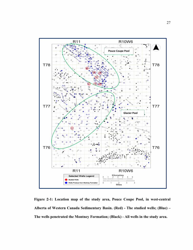
Figure 2-1: Location map of the study area, Pouce Coupe Pool, in west-central Alberta of Western Canada Sedimentary Basin. (Red) - The studied wells; (Blue) – The wells penetrated the Montney Formation; (Black) - All wells in the study area. ........................................................................................................................... 27

Figure 2-2: Log-correlations between the studied wells in the Pouce Coupe Pool, Alberta. Core facies of well 14-33-76-11W6 modified from Moslow & Davies (1997). ....................................................................................................................... 28

Figure 2-3: Composite-log in turbidite deposit (proximal turbidite lobe highlighted in yellow). GR, resistivity and density porosity responses over core intervals, well 13-12-78-11W6 (Modified from Pedersen, 2011). ................................................... 31

Figure 2-4: Core interval 2196-2213.22 m in well 13-12-78-11W6, consists of grey to light grey very fine grained sandstone, siltstone and shale. Siltstone thickness decreases upward from 4 to 1 cm; with an upward increase in sandstone and siltstone content. ....................................................................................................... 38

Figure 2-5: Core interval 2188-2206 m in well 5-14-78-11W6, consists of finely inter-bedded sandstone, siltstone and shale. Sandstone and siltstone thickness is variable throughout the core; with bed thickness ranging from 3 to 20 cm. Thickness of shale beds is decreasing up-ward from an average of 25 to 10 cm. .... 39

Figure 2-6: (A) Finely laminated planar and rippled siltstones. (B) thin-bedded siltstone to shaly-siltstone, 3- 15 cm thick, grade upward into climbing ripple laminations. (C) Planar laminated very fine-grained silty-sandstone to shaly-siltstone. (D) Fine siltstone and shale laminations. (E) Normally graded turbidite bed displaying planar laminations, grading upward into climbing ripple laminations, and capped by silty-shale bed. Siltstone and shale thickness ranges from 1-3 cm. .............................................................................................................. 40

Figure 2-7: GR, resistivity and bulk density logs responses over cored interval in well 13-12-78-11W6. Due to low resolution of conventional wire-line, thin beds cannot be detected. The blue areas are pores. Pores are irregularly distributed through the reservoir. ................................................................................................ 42

Figure 2-8: Comparison of XRD and Microprobe mineralogy analysis. Microprobe based on data from Freeman (2011). ........................................................................ 45

Figure 2-9: Cross-plot of RCA data between air permeability and porosity for the studied cores showing poor correlation. ................................................................... 48

Figure 2-10: Comparison between grain density and the porosity for the studied cores using RCA. Good correlation between grain density and core porosity was observed. ................................................................................................................... 49

Figure 2-11: Profile (probe) permeability measurements on slabbed core at ambient conditions, Well 13-12-78-11W6 (MnC Unit). ........................................................ 51

Figure 2-12: Plot of the porosity and permeability from ten core plug at ambient and various confining (overburden) pressures. ................................................................ 52

Figure 2-13: Plot of pulse-decay permeability measured at net ambient pressure versus pulse-decay permeability measured at reservoir net overburden (confining) pressure condition. ................................................................................. 54

Figure 2-14: Plot of probe (profile) permeability versus pulse decay permeability measured at net overburden pressure. ....................................................................... 54

Figure 3-1: GR & SGR logging responses over core interval, well 13-12-78-11W6....... 72

Figure 3-2: Clay distribution modes (From Dewan, 1983) ............................................... 72

Figure 3-3: Thorium-potassium cross-plot of Montney units from well 13-12-78-11W6 in western-central Alberta. The cluster of points is interpreted as illite. ....... 74

Figure 3-4: Thomas-Stieber cross-plot over core interval using well-logs data. The cross-plot indicates that structural and laminated shale are dominant type of shale/clay distribution. .............................................................................................. 75

Figure 3-5: Cumulative frequency plot of the studied wells. It shows that well 16-12-78-11W6 has less RHOB compared to the reference wells. (A) RHOB distribution before correction is applied; (B) RHOB distribution after correction is applied. .................................................................................................................. 77

Figure 3-6: ρmaa vs Umaa identification plot. Rock mineralogy and matrix were identified by the position of the data point relative to the points on the plot. (Black) – Thin section; (Red) – Microprobe and XRD. ........................................... 79

Figure 3-7: LDT & RHOB responses over the studied cores. As the LDT increases, RHOB increases. ....................................................................................................... 82

Figure 3-8: Nomograph for determination of matrix, porosity and the lithology proportions (from Gardner & Dumanoir, 1980). Average of Øta was 0.069 (red dot) by using average values of ρb & ØN Lst, which are 2.57 gm/cm3 & 0.067, respectively. Average of Øta was 0.077 (blue dot) by using average values of ρb & Pe, which are 2.57 gm/cm3 & 3.28 barn/electron, respectively. ........................... 83

Figure 3-9: Core analysis indicates that the grain densities average of 2696.1 kg/m3 for well 13-12-78-11W6. The average of the grain density for the well 5-14-78-11W6 is 2692.7 kg/ m3. ............................................................................................. 85

Figure 3-10: Correlation of the 27 sample points of core plug samples versus density and sonic porosity for unit MnC. .............................................................................. 86

Figure 3-11: Permeability increases when GR decreases. Interval of 2204.5-2207.5 m, uncertainties are associated of the relationship between GR and permeability in some depths. .............................................................................................................. 88

Figure 3-12: Spatial relationship between density porosity and permeability (covariance & correlation coefficient), well 13-12-78-11W6. ................................. 90

Figure 3-13: Comparison between density logs and log-derived porosity with routine core measurements (grain density, porosity and permeability), well 13-12-78-11W6. (A) Density log responses with core density, and (B) log porosity with core porosity and permeability. ................................................................................. 92

Figure 3-14: Comparison of density porosity with profile (probe) permeability. ............ 93

Figure 3-15: Cross-plot of core porosity versus density porosity. .................................... 93

Figure 3-16: Log-derived porosity versus permeability at reservoir net overburden pressure (NOB) for the core measured samples (27 samples), well 13-12-78-11W6. ........................................................................................................................ 95

Figure 3-17: Relative frequency (A), and cumulative frequency of the density porosity for the core interval (B). 63% of the porosity values are less than 0.06. .... 96

Figure 3-18: Histogram of permeability data (A), and a cumulative frequency of permeability (B) for the well 13-12-78-11W6 core. ................................................. 98

Figure 3-19: Effect of log transform on permeability histogram (A), and a cumulative frequency of log permeability (B). ............................................................................ 98

Figure 3-20: Conditional distribution of k against porosity bins for the studied core, well 13-12-78-11W6. ................................................................................................ 99

Figure 3-21: Comparison between core and log-based (Simandoux & Schlumberger) of water saturation estimates. Reasonable Sw values were obtained using the models for core, well 13-12-78-11W6. ................................................................... 102

Figure 3-22: Water saturation responses. Water saturation is higher in the shaly unit (MnD). Sw is higher in the MnD, which is might be less productive. .................... 104





Figure 4-1: Log-derived porosity versus permeability at reservoir net overburden pressure (NOB) for the core measured samples (well 13-12-78-11W6). ............... 123

Figure 4-2: Log-derived porosity versus permeability (7 points-averages) at reservoir net overburden pressure (NOB) for the core interval (well 13-12-78-11W6). ....... 123

Figure 4-3: Comparison of the estimated permeability with the core measurement permeability. Log-derived k values are either underestimated or overestimated. .. 124

Figure 4-4: Plot the measured values versus the estimated values for 27 measured samples (A), and for the entire core interval (B). ................................................... 125

Figure 4-5: Error versus measured value values for 27 measured samples (A), and for the entire core interval (B). ..................................................................................... 126

Figure 4-6: Cross-plot of the uncorrected probe permeability versus density porosity. . 129

Figure 4-7: Winland plot showing hydraulic rock types as a function of porosity, permeability and the dominant pore throat size. Although, the porosity values are

varied widely, only one hydraulic rock types were observed, which lies between the pore throat size of 0.05 and 0.1 micron for entire core interval. ....................... 129

Figure 4-8: Modified Lorenz Plot shows a cumulative storage capacity versus cumulative flow capacity from log derived porosity and profile permeability. (A) for the routine core data, (B) for log derived porosity versus 7 point average of profile permeability ................................................................................................ 131

Figure 4-9: Petrophysical characteristics of the cored interval Well (13-12-78-11W6). 132

Figure 4-10: Determination of the reservoir distribution using an integrated geological observations, core measurements and petrophysical properties. Most of the high permeability values are associated with the core lithology of very fine-grained sandstone and siltstones (petrofacies 3) and low values are from shale or shaly-siltstones (Petrofacies 1), Well 13-12-78-11W6. .................................................... 135

Figure 4-11: Log responses over the MnC interval, Well 13-12-78-11W6. Three petrofacies were recognized. Petrofacies 3 represent better reservoir properties. Petrofacies 1 has a lower reservoir quality. ............................................................ 136

Figure 4-12: Log responses over the MnC interval, Well 5-14-78-11W6. Three petrofacies were recognized. Petrofacies 3 represent better reservoir properties. Petrofacies 1 has a lower reservoir quality. ............................................................ 137

Figure 4-13: Log responses over the MnD interval, Well 13-12-78-11W6. Three petrofacies were recognized. Petrofacies 3 represent better reservoir properties. Petrofacies 1 has a lower reservoir quality. ............................................................ 138

Figure 4-14: Log responses over the MnD interval, Well 5-14-78-11W6. Three petrofacies were recognized. Petrofacies 3 represent better reservoir properties. Petrofacies 1 has a lower reservoir quality. ............................................................ 139

Figure 4-15: Electrical log correlation over Montney formation (MnC and MnD units) of the Pouce Coupe area in west-central Alberta. The composite-log responses do not easily detect the boundary between facies. In cores interval, Wells 13-12-78-11W6 and 5-14-78-11W6, the responses show increases in very fine sandstone and siltstone content by decrease in GR signatures. .............................. 142

Figure 4-16: Cutoff value estimation using the relationship between permeability and porosity for the core samples. The dotted lines indicate the standard error band of (± 0.00066 mD). ................................................................................................. 144

Figure 4-17: Comparison of the computed log permeability and measured permeability, Well 13-12-78-11W6. The Net-to-Gross ratio has been estimated by using porosity and permeability parameters. ..................................................... 147

Figure 4-18: Relationship of porosity with vertical and horizontal permeability. .......... 151

Figure 4-19: Vertical-horizontal permeability relationship in the studied wells. ........... 151

Figure 4-20: Permeability is related to porosity, as the porosity increases, the permeability increases. High GR accompanies low permeability. This may suggest narrow pore radius due to pore lining/bridging clay. ................................. 156







Figure 4-27: Permeability is related to porosity, as the porosity increases, the permeability increases. High GR accompanies with low permeability. This may suggest narrow pore radius due to pore lining/bridging clay. ................................. 163

List of Symbols, Abbreviations and Nomenclature

Symbol Definition

MnFM Montney Formation MnD Montney Formation (unit D) MnC Montney Formation (unit C) TS Thin section SP Sample Point OM Organic matter, weight % FU Flow Unit K Potassium, percentage Th Thorium, Part per Million (ppm) Ur Uranium, Part per Million (ppm) Ø Porosity, fraction or percentage Vb Bulk volume of the reservoir rock, fraction Vgr Grain volume, fraction Vp Pore volume, fraction u Fluid viscosity, cm/s q Flow rate, cm3/s k Permeability, darcy (D) or milli-darcy (mD) Ac Cross-sectional area of the rock, cm2 µ Viscosity of the fluid, centipoise (Cp) l Length of the rock sample ∆p Pressure gradient, atm or KPa/m Pr Reservoir pressure, psia PR Poission’s ratio, dimensionless Ish Shale index Vsh Shale volume, fraction or percentage γlog Gamma ray of intrested zone, API γsh Gamma ray of shale zone, API γc Gamma ray of clean zone, API ρb Bulk density, cm/gm3 or kg/m3 ρf Fluid density, cm/gm3 or kg/m3 ρma Matrix density, cm/gm3 or kg/m3 c(l) Covariance, dimensionless r(l) Correlation coefficient, dimensionless Sw Water saturation, fraction or percentage n Saturation exponent Ro Rock resistivity, ohmm F Formation resistivity factor a Tortuosity factor Rw Water resistivity, ohmm m Cementation factor Rt Bulk resistivity, ohmm Rsh Shale resistivity, ohmm

Øe Effective porosity, fraction or percentage ρmaa Apparent matrix density, gm/cm3 or kg/m3 Pe Photoelectric absorption indexes,

barn/electron Uf Fluid volumetric cross section ρe Electron density index Øta Apparent total porosity, fraction or percentage ∆mtx Matrix transit time, sec/m ∆fl Pore fluid transit time, sec/m Rp35 Pore size measurements at 35% mercury

saturation Øc Porosity cut-off value, fraction or percentage Kc Permeability cut-off value, D or mD k/Ø Delivery speed Øh Cumulative storage capacity Kh Cumulative flow capacity NTG Net-to-Gross ratio Ke Effective permeability, darcy or milli-darcy he Effective pay thickness, m or feet OGIP Initial-gas-in-place, scf Bgi Average initial formation volume factor, cf/scf Zi Compressibility, psi-1 Pi Initial pressure of the gas reservoir, psia T Temperature, Fehrenhite (F°) or Rankin (R°) GR Gamma ray, API RHOB Bulk density, kg/m3 or g/cm3 Res. Resistivity, Ohm-m KBE Permeability cut-off for best estimation, mD CGT Core gross thickness, m or ft NST Net thickness, m or ft NsTCG Net-to-gross core thickness NPT Net pay thickness, m or ft KH Horizontal permeability, mD KV Vertical permeability, mD T-C Type-Curve method S-L Straight-Line method G Gas C Condensed Gas W Water

1

INTRODUCTION Chapter One:

Introductory Statement, Objectives and Scope of the Project 1.1

Producing gas economically from unconventional reservoirs with the increasing

demand and diminishing gas production from conventional reservoirs is a challenge.

Unconventional gas resources (UGRs) such as shale gas, coal-bed methane, and tight gas

constitute a significant percentage of the natural gas resource base and offer significant

potential for future reserve growth and production (Newsham & Rushing, 2001).

Unconventional gas reservoirs are characterized by complex geological

heterogeneities at all scales and exhibit the unique gas storage and flow properties.

However, they are difficult to develop. A fundamental problem for the UGRs includes

the estimation of the gas and fluids storage and distribution. Consequently, the efficient

development of the UGRs requires careful characterization of the resource.

Understanding the controls of the rock type, petrophysical properties, pore size,

permeability, flow units, and the improved technology is the key to the commercial

success in the UGRs.

Recent advances in technologies such as horizontal drilling, completion, hydraulic

fracturing, and production technology have allowed for the commercial exploitation of

ultra-low permeability natural gas reservoirs, where hydrocarbon flow-rates and

recoveries achieved by using conventional technology was historically too low to be

economical to the producer.

This research was conducted within the context of the Unconventional Reservoir

Analysis in Western Canada (URAWC) research group as well as the Centre for Applied

Basin Studies (CABS) in the department of geosciences, University of Calgary.

2

The aim of the project is to develop a methodology to evaluate, and predict the

reservoir performance in a complex, finely laminated tight gas reservoir by using

petrophysical methods when the reservoir sample data are limited. Two geologic informal

units, the Montney C (MnC) and Montney D (MnD), will be discussed in this research.

The ability to predict permeability (k) and flow (hydraulic) units (FU) within

heterogeneous reservoirs remain difficult. A flow unit is defined as a reservoir

subdivision characterized by a similar pore type (Hartmann and Beaumont, 1999); it is a

zonation that is recognizable on well logs and; may be in communication with other flow

units (Tiab & Donaldson, 2004). Utilizing the flow unit identification during the reservoir

characterization process allows us to better understand the distribution of the reservoir

properties (layering).

The purpose of the current study of the Montney Formation will focus on five

elements:

1) Characterization of the Montney reservoir in the Pouce Coupe field and

discussion of the degree of heterogeneity;

2) Analysis of core samples, and the well logs to determine the reservoir

properties, and application of advanced methods for the log-core calibration;

3) Development of a correlation between permeability and well log responses to

identify the permeability distribution and prediction of the flow unit properties in wells

having only well log data;

4) Discussion and analysis of various issues related to the net pay evaluation and

resource estimation using well logs;

5) Comparison of reservoir ( ) derived from well log, and production data;

3

The focus of this study is on the Lower Triassic of Montney Formation (MnFM)

in Pouce Coupe field of west-central Alberta within the Western Canada Sedimentary

Basin (WCSB). Although the conventional Montney reservoirs have been exploited for

decades, recent industry has been focused on the “unconventional” Montney reservoir in

the western WCSB, where the Montney is more shale-prone and over-pressured (Jones et

al., 2008).

Literature Review 1.2

Natural gas produced from the unconventional tight gas sands reservoirs could

significantly contribute to the known gas reserves. The Geological Survey of Canada has

made an attempt to verify and evaluate the gas-in-place (OGIP). The gas resource base of

the tight sands is estimated to be 90-1500 tcf (trillion cubic feet) in Canada and 7500 tcf

around the world (Aguilera & Harding, 2007).

While the OGIP is large in Canada, only a portion of these resources are

recoverable (between 230-590 tcf), with half being attributed to the Deep Basin and the

Montney Formation in Alberta, and the rest to various accumulations in northeastern

British Columbia (CSUG, 2011).

The Triassic Montney tight unconventional gas (tight gas/shale) is amongst the

recent targeted natural gas reservoirs in the WCSB, and continues to be an active

exploration play. The MnFm thicknesses range from 50 to 350 m, the formation covers

approximately 35,000 square miles, and the geology of the MnFM is extremely complex

and variable (Panek, 2000). The Montney is expected to produce approximately 9% of

the total Canadian natural gas production by 2020 (Gatens, 2009).

4

The original gas in place estimates in the Lower Triassic Montney Formation of

west-central Alberta vary from 80 to 700 tcf, of which only a fraction may be recoverable

(approximately 20%). The natural gas production from the individual horizontal wells

drilled in the MnFM varies from 85,000-141,000 m3/day (3-5 MMcf/day) (NEB, 2009).

Difficulties in the reservoir characterization include: i) the used routine lab-based

methods for permeability measurements. The permeability of the Montney is below the

resolution of the routine analysis instruments; ii) the proper estimation of the complex

pore size distribution in order to quantify the gas and fluid capacity due to the diagenesis;

iii) development of the relationship of the tight gas sand reservoirs between the matrix

and hydraulic flow, especially for low permeability reservoirs such as the MnFM.

The prediction of well performance in heterogeneous tight reservoirs historically

has not been entirely successful. Due to fact that each tight sandstone reservoir has

different properties, each reservoir should be considered as a research project in itself. As

a result, there are different approaches that have been used to understand and develop

some useful interpretations of such unconventional reservoirs.

Petrophysical analysis has increasingly become a part of the work performed by

geologists, geophysist and engineers. Interpretation methods and approaches are

continually changing. Understanding the limitation of conventional log analysis when

applied to tight gas sands can produce better results.

Therefore, the integration of lab analysis such as thin sections (TS); x-ray

diffraction (XRD); scanning electron microscopy (SEM); core measurements such as

porosity, permeability, and water saturation; wire-line logs such as gamma ray, density,

5

resistivity along with well production data is a good approach for reservoir

characterization.

An integrated approach to the calibration of the lab data, cores with well log data

to define the rock types, permeability prediction, flow unit identification, net pay

estimation can also improve the characterization and can predict the performance of the

reservoir (Rushing et al., 2008).

Geostatical models and simulation can be used to reduce the errors and

uncertainty in the evaluation of the reservoir distribution field-wide. In addition,

graphical methods such as Winland porosity-permeability cross plot, delivery speed, and

Modified Lorenz Plot (MLP) can be applied for quantifying the reservoir flow units

based on the geological framework, petrophysical rock/pore type, storage and flow

capacity (Balan et al., 1995).

A comprehensive literature review was conducted on the tight gas in sandstone,

shale and carbonate reservoirs and their heterogeneity. There have been many different

approaches to quantifying the reservoir properties such as porosity, permeability, water

saturation. Furthermore, no single method has emerged as the definitive basis for

delineating the net pay and reservoir characteristics in such unconventional reservoirs.

Only the key issues in the evaluation of the reservoir characteristics, petrophysical

properties, permeability prediction and net pay estimation of the tight sandstone gas

reservoirs are considered in this study. Table 1.1 shows a list of the petrophysical texts

books and technical literature discussed in the research.

6

Table ‎1-1: List of examples of integrated reservoir characterization. (L) Lab, (C)

Core, Core cutting (Lg) Logs, (WT) Well tests, (Øc) Porosity cut-off value, (kc)

Permeability cut-off value

Investigators Reservoir Characterization

Heterogeneity k Evaluation & Flow Unit

Net Pay Parameters

L C Lg C Lg WT Øc Kc

Pirson (1958) * *

Calhoun (1960) * *

Makenzie (1975) * *

Kukal et al. (1983) * *

Delfiner et al. (1987) * *

Howell et al. (1992) * * *

Ameri et al. (1993) * *

Yao & Holditch (1993) * * *

Feitosa et al. (1993) *

Molnar et al. (1994) * *

Balan et al. (1995) * * *

Mohaghegh et al. (1995) * * *

Gunter et al. (1997) * * * * * *

Gunter et al. (1997) * *

Saner et al. (1997) * * *

Deakin & Manan (1998) *

Flolo et al. (1998) * * * *

Davies et al. (1999) * * * * *

Revil & Cathles (1999) * * *

Newsham et al. (2001) * * *

Rushin et al. (2001) * * *

Hopkins & Meyer (2001) *

Marquez et al. (2001) * *

Shanley et al. (2004) * * *

Jensen & Menke (2006) * *

Florence et al. (2007) * *

Rushing et al. (2008) * * * * *

Jacobi et al. (2008) * * *

Aguilera (2010) * *

Kale et al. (2010) * * * *

Clarkson & Beierle (2010) *

Pankaj & Kumar (2010) *

Sondergeld et al. (2010) * * *

Clarkson & Jensen (2011) * * * * * *

7

Geology Background 1.3

This chapter discusses the geological background, and reservoir characteristics of

the Montney Formation (MnFM) in west-central Alberta. The Lower Triassic Montney

Formation was named by Armitage (1962). This study focuses on the Montney

Formation, Pouce Coupe region of west-central Alberta, Canada, where the

unconventional tight gas reservoirs are comprised of siltstone/shale.

Regional Structure and Tectonic Setting 1.3.1

In the Triassic time, the WCSB was located on the northwestern margin of the

supercontinent Pangea, facing the Panthalassa Ocean. There were no major tectonic

events that deformed the accumulating sedimentary wedge in the adjacent continental-

margin, extensional Triassic basin (Davies & Sherwin, 1997). Sedimentation in WCSB in

the Triassic time was confined to three tectonically controlled contiguous basins, which

are the Peace River Basin, Continental Margin Basin and the Liard Basin (Davies et al.,

1997).

The study area overlies the southeastern margin of the collapsed Peace River Arch

as defined by (Barclay et al., 1990), and northeast trending Upper Devonian Leduc Reef

Figure 1.1. The second major structural element in the study area is the southern

extension of the Fort St. John Graben (Barclay et al., 1990)

8

Figure ‎1-1: Location of the study area and paleogeography setting of the Lower

Triassic Montney Formation in Alberta and northeastern British Columbia. Top

left picture (Pedersen, 2011), middle left (Zaitlin & Moslow, 2006), top right

(Zonneveld et al., 2011), bottom picture (Moslow, 2000).

Study Area

Pangea

Pouce Coupe

Pan

thal

assi

c O

cean

9

Stratigraphy and Sedimentology 1.3.2

The Triassic stratigraphic framework of the WCSB has been established by

outcrop mapping and subsurface work over several decades (Gibson, 1975). Gibson &

Edwards (1990b) have interpreted the entire Triassic succession as comprising three

transgressive cycles.

The first cycle comprises the early Triassic Grayling, Toad and Montney

formations. The second cycle consists of the middle to early late Triassic Liard, Doig and

Chalie Lake formations, and the last cycle is composed of late Triassic Baldonnel,

Pardonet and Bocock formations.

Each cycle contains rocks deposited in a marine shelf setting ranging from the

distal deep shelf waters to proximal shoreline. The main nomenclature used for the

Triassic strata in the WCSB is shown in Figure 1.2. In west-central Alberta, the Montney

unconformably overlies the Permian Belloy Formation, but it overlies older Paleozoic

(Mississippian) strata in other areas. The Montney Formation is overlain by the Middle

Triassic Doig Formation.

In the eastern part of the Peace River area in west-central Alberta, the Montney is

overlain unconformably by the Worsley Member of the upper Charlie Lake Formation.

Where the Worsley is absent, the truncated Montney is overlain unconformably by

bituminous shale of the Jurassic Fernie Formation (Nordegg Member) (Davies, 1997a).

10

Figure ‎1-2: Regional Triassic stratigraphy framework, facies and equivalent strata

in the WCSB (from Davies, 1997b).

Lithostratigraphic divisions of the Triassic Montney Formation were discussed by

the previous authors. Davies et al. (1997) subdivided the Montney succession into three

informal members based on a part of the Montney’s occurrence between townships 70 to

86, from R22W5 to R12W6 in west-central Alberta. The dominant lithologies in the

MnFM are silts and shale. The MnFM is divided into upper and lower members; a middle

member consisting of coquinal dolomite is present in the east Figure 1.3.

11

The Lower member of the Montney consists of coarsening-upward, very fine

grained sandstones and siltstones. The base of the Lower member overlies the Permian or

the Paleozoic strata, while the top is marked by a coquina dolomitic member in the east,

or by a sequence boundary below the Upper member to the west. The volume percentage

of the sandstone in the east is about 30%, whereas it is about 10% in the west, suggesting

an eastern source of the Montney (Lee, 1999).

Thick dolomitized coquina of the middle member is underlain by the Lower

member of the Montney through a north-to southwest-trending belt in the eastern

subsurface of west-central Alberta. It occurs over a limited east-west extent and a more

extensive north-south distribution (Dixon, 2000). The coquina bed was deposited in

shallow water, oxygenated environment dominated by bivalve mollusks (Davies &

Sherwin, 1997).

The upper member of the Montney overlies the Coquinal Dolomite Middle

member in the eastern shelf, or a disconformity in the west. The upper Montney member

is generally characterized by coarsening-up siltstones with very fine grained sandstones

and dolomitized coquina facies occurring locally. The top of the Upper member, where

not eroded, is overlain by the Doig Formation (Davies, 1997a).

In the Valhalla area, the distinction between the lower and upper members

becomes less distinct due to the lithological similarity. Dixon (2000) has added a shale

member to the three members in the westward due to a not well-defined Coquinal

Dolomite member. He designated a siltstone-sandstone member, overlain by a shale

member Figure 1.3.

12

Figure ‎1-3: Geological members of Montney Formation. By Dixon (2000), lower

member (siltstone-sandstone), middle member (coquinal dolomite), upper member

(siltstone), and (shale) member. Top picture (Pedersen, 2011), bottom picture

(Dixon, 2000).

There are few detailed sedimentological studies of the MnFM. Miall (1976)

interpreted that the coarser grained siltstone, sandstone and coquina facies close to the

eastern depositional margin were deposited in shallow water, deltaic environment.

13

Moslow & Davies (1997) suggested that a sea level fall enhanced the mass-

wasting processes and generated the sediment gravity flows resulting in the deposition of

turbidites. They suggested that the turbidite deposition took place at the toe of the slope

with the contemporaneous deposition of the coquina beds on the shoreface during a

progressive fall at sea level and/or at a lowstand at sea level.

Davies et al. (1997) reported that the offshore shelves were dominated by the

storm processes and turbidities accumulated the down-slope or at the toe of the slope

setting within the northeast-southwest trending channels. A wide range of depositional

environments in the MnFM is recorded by facies ranging from mid to upper shoreface

sandstones, to middle and lower shoreface sandstones and coarse siltstones, to finely

laminated lower shoreface sand and offshore siltstones, and to siltstone/shale turbidites.

Moslow (2000) documented that the MnFM has multiple para-sequences of very

fine grained sandstone, siltstone and mudstone (shale). Within the eastern portion of the

WCSB, the boundary between the lower and upper MnFM is demarcated by laterally

discontinuous dolomitic coquina beds, which forms a retrogradational shoreface

succession. To the west, the lowstand system is presented by two sequences composed of

the turbidite sandstone/siltstone and the shale facies Figure 1.4.

Within the turbidite succession, five siliclastic sedimentary facies have been

recognized based on the lithology, texture, and sedimentary structures. The facies are a

product of the turbidity current processes of the deposition. The facies are (a) Turbidite

Channel Sandstone; (b) Tubidite Channel Margin Sandstone and Siltstone; (c)

Levee/Overbank Sandstones, Siltstone and Shale; (d) Turbidite Lobe Silty to Shaly

Sandstone; (e) Distal Shelf Siltstones and Shales (Moslow, 2000) Figure 1.5.

14

Figure ‎1-4: Schematic simple west-east of Lower Triassic Montney Formation facies

(from Moslow, 2000).

Figure ‎1-5: Lateral variation of turbidite facies from the proximal to the distal for

the Montney Formation The letters a-e represents the Bouma sequence. CCC

referred to the “Climbing ripples, Convolution and Clasts” (from Moslow, 2000).

15

Petroleum Play Systems 1.3.3

Master (1979), Law (2002) and Naik (2007) conducted detailed studies of the

Cretaceous Basin Centered Gas Systems (BCGS). As the source and reservoir rocks

undergo further burial and exposure to the increasing temperatures, the source rocks

begin to generate hydrocarbon.

With increased gas generation, expulsion, and migration, gas begins to enter the

adjacent siltstones/fine-grained sandstones. Due to the low permeability of the

sandstones, the rate of gas generation is greater than the rate of gas lost with little or no

free water. It is likely that the petroleum systems play for the MnFM is similar to the

BCGS petroleum system play.

Conventional and/or unconventional hydrocarbon exploration requires in part the

presence of organic-rich, thermally-mature source rocks containing oil or gas prone

kerogen. Hankel & Riediger (2001) suggested that the lower Montney siliciclastics

represent poor to good source rocks based upon the Total Organic Carbon (TOC) content.

In general, the Lower Triassic Montney Formation contains Type II/III kerogen

with TOC range from 0.51 to 4.18 wt. %, suggesting that this unit generated a significant

amount of hydrocarbons where it is thermally mature (Jones et al., 2008). TOC of the unit

MnC was obtained in range of 0.6 to 0.8 wt. %, whereas the TOC of MnB was in range

of 1.1 to 1.8 wt. % (Leyva et al., 2010).

Porosity and permeability 1.3.4

The measure of fluid (oil, gas, water) trapped within the void space of the rocks is

known as the porosity. The porosity is the void volume divided by bulk volume. The

ability of the fluid to flow is known as permeability. Knowledge of these parameters is

16

essential to evaluate the types of flow, their quantities and fluid recovery.

Mathematically, porosity can be expressed as:

(‎1-1)

Where, ( ) is porosity, fraction, ( ) bulk volume of the reservoir rock, ( ) grain

volume, ( ) pore volume

In general, the factors controlling porosity are: i) grain size and sorting

(uniformity); ii) cementation; iii) compaction during and after deposition; iv) grain

packing. Porosity can be classified into primary porosity such as inter-granular and inter-

crystalline, and secondary porosity such as fracture porosity, solution porosity (Tiab &

Donaldson, 2004). Quantitatively, porosity is used for the reserve estimation (volumetric

method).

Permeability on other hand depends on the effective porosity (connected voids). It

is affected by the grain size; pore throat size; degree of cementation; and clay type.

Permeability can also be classified into primary permeability (matrix permeability); and

secondary permeability (fracturing, solution). Mathematically, the permeability expressed

as the following:

(‎1-2)

Where, ( ) is fluid viscosity, cm/s, ( ) flow rate, cm3/s, ( ) permeability, Darcy

(0.986923 m2), ( ) cross-sectional area of the rock, cm2, ( ) viscosity of the fluid,

centipoise (Cp), ( ) length of the rock sample, (

) pressure gradient in the direction of

the flow, atm/cm

17

The “relationship between the porosity and permeability is qualitative and is not

directly or indirectly quantitative” (Tiab & Donaldson, 2004). Conventional reservoirs

are characterized by higher porosity and permeability, and the wells generally recover a

greater percentage of the hydrocarbon-in-place. However, in unconventional reservoirs,

similar geological and petrophysical properties must be distinguished for a better

correlation between the porosity and permeability.

High porosity shore-face sands (eastward) become less porous and permeable

westward and down-dip, passing from the water-bearing area with local gas traps through

a transition zone to a gas-bearing area. The conventional shore-face sand reservoirs of the

siliclastic facies in the up-dip have porosity in the 10 to 15% range, and permeablities in

the 0.7 to 80 millidarcy (mD) range (Davies et al., 1997).

The porosity and permeability values from the conventional core analysis of the

Montney reservoir in west-central Alberta demonstrate that the dolomitized coquina

facies have the highest overall porosity and permeability, with most values in the 12 to

22% porosity range and 20 to 1000 mD of permeability range (Davies et al., 1997).

The porosity and permeability decreases westward and down-dip into the fine-

grained deposits. In general, in the deep basin, part of the WCSB of tight gas sands have

permeabilities less than 0.1 mD relatively low porosity with an average of 6.7%, and an

average water saturation of 40% (Zaitlin and Moslow, 2006).

Unconventional reservoirs produce gas from ultra-low permeability resources of

less than 0.001 mD to a high of 0.1 mD (permeability cut-off value for tight gas). At the

westward limit of the Alberta Deep Basin, the porosity and permeability decrease

because of the clay content in more deeply-buried sediments, cementation, and diagenesis

18

(Zaitlin & Moslow, 2006). In general, porosity and permeability values vary greatly for

the different sediment facies of the Montney.

Understanding gas production from low permeability rocks requires an

understanding of the petrophysical properties-lithofacies associations, facies distribution,

gas permeabilities at reservoir conditions, and the architectural distribution of these

properties. Advanced drilling, completion and stimulation methods are required to

achieve the commercial production in the unconventional Montney play (Thompson et

al., 2009). The tight gas in the MnFM is now being exploited with horizontal wells,

stimulated by using the multiple hydraulic fracture stages.

Methods 1.4

The methods for assessing the variability and structure of the reservoir properties

of geological units are applied to the measurements at various scales. The methods are in

an increasing scale from the probe permeameter, core plugs data, full diameter core, and

wire-line logging tools up-to production data. All the core measurements have been done

by ®CoreLab. The method uses an integrate cores and log-derived data Figure 1.6.

19

Figure ‎1-6: Schematic diagram of the procedures used for characterizing the

Montney reservoir.

Proposed Method

Cores, Core Analysis Results Composite of Well Logs

Vsh, Ø, Sw

Correlating and Matching Wire-line Logs to Cores Analysis

Petrofacies (Electrofacies)

Flow (Hydraulic) Units Identification

Net Pay Estimation

Permeability Prediction

Integrate Static Ø to Dynamic Properties k

OGIP Reserve Calculation

Compute Statistical Measures of all variable (Avg., SD, Cv, Histogram, Normality Test, Error Analysis)

Sample Analysis, Thin Section, XRD GR, RHOB, Resistivity

Comparison Log derived k to Well-Test derived k

Winland, MLP K-Ø Correlation

Øcutoff, Kcutoff, Swcutoff Vlaues

Lithology, Grain Size, Sed. Structure – k, Ø, Sw

20

Core Analysis 1.4.1

Of the five (Montney) studied wells, two cores were examined within the studied

area; analysis included core log descriptions and measurements. Only a small number of

the wells in the studied area were cored whereas all wells were logged. Cores allow for

the direct evaluation of the reservoir properties and provide a basis for calibrating other

evaluation tools such as well logs.

Core data are used to describe the lithology and to determine the reservoir facies.

Consequently, the cores selected for this analysis were used to assess both the lateral and

vertical facies variability in order to estimate the reservoir properties within the study

area, along with the calibration of the well logs. The actual vertical position of the core

must be adjusted through the correlation with the wire-log responses.

Core analysis data were performed by ®CoreLab. Routine Core Analysis (RCA)

including porosity, air permeability, grain and bulk density, and water saturation where

available from a full diameter analysis of both cores. Helium porosimetry was used to

establish the porosity, and steady-state measurements at a confining pressure of 3.45 MPa

(500 psi) net confining pressure performed to obtain the permeability.

The bulk volume measurement was caliper-based, and the water saturation was

obtained from the Dean Stark distillation. The RCA procedures are inadequate for the

tight gas because it cannot capture the heterogeneity changes at a fine scale. As a result,

some trends from the RCA may not be observable.

The profile permeameter data were collected for one of the studied cores at 2.5

cm (1 inch) intervals. These data were collected to quantify vertical heterogeneity in

permeability in one of the producing interval (Clarkson et al., 2011). Core plugs were cut

21

at the location of the selected probe permeability measurement points for further analysis

including the pulse-decay permeability and porosities measured at the confining pressure

representative of the reservoir (Jones, 1997).

The profile permeability measurements were correlated to pulse-decay

permeability measured data to allow adjustment of the profile data to in-situ stress

conditions (Clarkson et al., 2011). Finally, permeability and porosity relationships were

generated by using the adjusted profile permeability and porosity estimates from the logs

were used to estimate pore throat aperture, to delineate flow units zones, to estimate the

net pay and evaluate the gas reserves.

Wire-line Log Evaluation 1.4.2

The focus of this study is a well log analysis of the Lower Triassic Montney tight

gas interval in a portion of the Pouce Coupe Field. Well logs are continuous records of

geophysical parameters (electric or radioactive parameters) along a borehole. Well logs

can be important tools for determining reservoir zonation, differentiating between the

shale and sands, or between the porous and less porous facies.

Fluid saturation and productivity depend on facies and diagenetic alterations that

control connectivity and heterogeneity of the flow units. Correlation of the well logs

responses to core is necessary to accurately derive the reservoir properties in the wells

that have not been cored.

To reduce the uncertainty in the estimation of the reservoir properties in tight gas

reservoirs, it is essential to integrate the core and log data. In this study, logs were

calibrated to core for better definition of the petrophysical properties. Successful

22

application of this approach may play a critical role in the exploration and development

decision-making processes for tight gas reservoirs.

Reservoir properties of the different facies, such as shale volume, porosity and

fluid saturation, can vary significantly. These variations have led to further subdivision

known as flow units based on the measured permeability. Eventually the porosity was

correlated to the permeability for the permeability prediction of un-cored intervals. As a

result, the net thickness was estimated and, consequently, the absolute permeability of the

matrix was evaluated from (kh).

Statistical Analysis 1.4.3

Statistics and/or geostatistics can provide a quantitative description of the

variability of natural parameters such as porosity with permeability in porous media.

Generating the gas production rates and the reserve recovery estimates for the

unconventional reservoirs in the MnFM and it is not an easy task since its flow behavior

is not fully understood.

When a reservoir is heterogeneous, a subdivision of the geological succession

based on different facies is needed. The porosity versus permeability relationship and cut-

off values should be considered facies by facies based on a petrophysical, geological and

engineering criteria. Each of the petro-facies units can have a different set of parameter

relationships and cut-off values.

Even where a reservoir comprises a single petrophysical rock type, different

cutoffs may need to be applied in different parts of the reservoir due to the different

dynamic properties associated the reservoir such as mobility, and hydrocarbon properties

(Worthington and Cosentino, 2005).

23

Production Data 1.4.4

Production and well log data can be powerful tools for evaluating the performance

of a well. For example, permeability estimated from logs can be correlated to the

estimates from the production data. The correlation can be used to evaluate the potential

productivity. During a production test, sizable samples of formation fluid are recovered.

The recovery of fluids depends on the porosity (storage) and permeability (transmit) of

the formation tested and gas properties contained in the studied units.

Better understanding of the relation between cores, well logs, production data

analysis (PDA) and pressure transient analysis (PTA) allow us to obtain the

representative conductivity distributions as part of the reservoir characterization from the

fluid flow measurements.

An estimate of the average formation permeability ( ) can be conducted with

open-hole well logs analysis as described in the equation (below). A rigorous estimate

can be obtained by minimizing the difference between the calculated and estimated

permeability values from PDA/PTA (Poe & Butsch, 2003). The (kh) values from the well

logs will be compared to PTA or PDA derived values.

∑ (‎1-3)

Where, (kj) and (hj) are the individual interval formation conductivity and thickness,

respectively

24

GEOLOGICAL RESERVOIR CHARACTERIZATION Chapter Two:

Introductory Discussion 2.1

The Lower Triassic Montney Formation (MnFM) in the study area is a complex

succession consisting of shale, siltstone and very fine-grained sandstone. Deposition of

the MnFM occurred in a wide variety of depositional environments, from distal offshore

successions including the turbidite channel and fan complexes to lower to upper shore-

face deltaic (Davies et al., 1997; Moslow, 2000; Panek, 2000; Zonneveld et al., 2011).

Study Area 2.2

The area of this study is located in the subsurface from approximately (55° to 56°

N) latitude and (119° to 120° W) longitudes. This investigation provides a summary of

the results from the petrophysical analysis of the Lower Triassic Montney Formation

within Township of 78, Range R11W6, from Section 2 to 14. The selected wells covered

an area of 1546.448 Acres (625.825 Hectares, 67363258.511 ft2 or 6.258 Km2).

The five studied wells penetrated to the base of the MnFM within the Pouce

Coupe Pool, and of these, two wells were cored in the MnFM, which are 13-12-78-11W6

and 5-14-78-11W6 Figure 2.1. In addition, there are many geophysical well logs

currently available within the study area from the oilfield drilling operations targeting the

Montney Formation and other targets formations including the gamma ray, bulk-density,

resistivity, and porosity logs.

Well 14-33-76-11W6 was used as a reference well for the correlation of the

studied wells. The well was correlated with the wells in the Glacier Pool of the paper

published by Moslow & Davies (1997). Well 14-33-76-11W6 core shows the turbidite

25

lobe facies association in the Glacier field. Correlation of the studied wells is shown in

Figure 2.2.

Two wells 16-12-78-11W6 and 3-12-78-11W6 have been selected to represent the

producing wells from the MnFM. These wells will be used to compare with the other

wells that are not producing from the MnFM in the study area. On the other hand, Well

2-2-78-11W6 was selected as a well in the study area that penetrates the MnFm but does

not produce from it. It produces from the Triassic Doig Formation.

In addition, two wells, 1-1-78-11W6 and 3-1-78-11W6 were selected to compare

the production from these wells to the producing wells 16-12-78-11W6 and 3-12-78-

11W6. Well 1-1-78-11W6 is co-producing from the Lower Montney Formation, the

middle Triassic Doig formation and the Lower Cretaceous Gething Formation.

The Lower Cretaceous Gething Formation is comprised of a conglomerate,

sandstone, coal, siltstone and shale. It overlies the Cadomin Formation and is overlain by

the Bluesky Formation (Hubbard et al., 1999). The Middle Triassic Doig Formation

consists of siltstone, shale and nodular phospahates occurs at the base of the formation

(Chau & Henderson, 2010). Table 2.1 summarizes the studied wells information.

26

Table ‎2-1: Well information (source: geoSCOUT geoLOGIC Systems &

AccuMapTM, 2011)

Well ID Location Core Interval (m) Montney Formation (MnFM)

Remarks

Lat. (°N) Long. (°W)

Top (m) Base (m)

100/13-12-78-11W6 55.75 119.75

2196.0 – 2214.0 (18 m)

1997.0 2289 (TD)

Core (MnC & MnB), logs (GR, Res., Bulk-density, Porosity), year

drilled (2008), Production FM (TRmontney),

Central Pouce Coupes

100/5-14-78-11W6 55.76 119.59

2188.0 – 2206.0 (17.4 m)

1991.0 2261.8 (TD)

Core (MnC), logs (GR, Res., Bulk-density, Porossity), year drilled

(1992/93), Production FM (Kgething, TRdoig, TRmontney),

East-Central Pouce Coupes

102/16-12-78-11W6 55.75 119.55

- 1979.6 2230 (TD)

Logs (GR, Res., Bulk-density, Porosity)

, production data, year drilled (2003), Production FM

(TRmontney), Central Pouce Coupes

100/3-12-78-11W6 55.74

119.56 - 2011.2

2265 (TD) Logs (GR, Res., Bulk-density,

Porosity) , production data, year drilled

(2006), Production FM (TRmontney),

Central Pouce Coupes

100/2-2-78-11W6 55.72 119.58

- 2005 2277.3

Logs (GR, Res., Bulk-density, Porosity), year drilled (1994),

Production FM (TRdoig), Central Pouce Coupes

100/14-33-76-11W6 55.63

119.64 - 2197.5

2466.3 GR, Res., Bulk-density, Porossity),

year drilled (1983), Production FM (TRmontney, TRdoig),

Lahee (Reference well for the correlation)

100/1-1-78-11W6 55.72

119.55 - 2040.2

2293 (TD) GR, Res., Bulk-density, Porossity),

year drilled (2005), Production FM (Kgething, TRmontney,

TRdoig), Lahee (Production well)

102/3-1-78-11W6 55.72

119.56 - 2018.0

2271 (TD) GR, Res., Bulk-density, Porossity),

year drilled (2005), Production FM (TRmontney),

Lahee Production well)

27

Figure ‎2-1: Location map of the study area, Pouce Coupe Pool, in west-central

Alberta of Western Canada Sedimentary Basin. (Red) - The studied wells; (Blue) –

The wells penetrated the Montney Formation; (Black) - All wells in the study area.

123456

7 8 9 10 11 12

131415161718

19 20 21 22 23 24

252627282930

31 32 33 34 35 36

123456

7 8 9 10 11 12

131415161718

19 20 21 22 23 24

252627282930

31 32 33 34 35 36

123456

7 8 9 10 11 12

131415161718

19 20 21 22 23 24

252627282930

31 32 33 34 35 36

123456

7 8 9 10 11 12

131415161718

19 20 21 22 23 24

252627282930

31 32 33 34 35 36

123456

7 8 9 10 11 12

131415161718

19 20 21 22 23 24

252627282930

31 32 33 34 35 36

123456

7 8 9 10 11 12

131415161718

19 20 21 22 23 24

252627282930

31 32 33 34 35 36

T76

T77

T78

T76

T77

T78

R10W6R11

R10W6R11

0 1 2 3 4 5 6

0 1 2 3 4

Kilometres

MilesWells Produce from Montney FormationWells Produce from Montney Formation

Studied WellsStudied Wells

Selected Wells LegendSelected Wells Legend

Pouce Coupe Pool

Glacier Pool

28

Figure 2-2: Log-correlations between the studied wells in the Pouce Coupe Pool, Alberta. Core facies of Well 14-33-76-11W6 from Moslow & Davies (1997).

0.00 150.00GR (GAPI)

0.00 150.00HCGR (GAPI)

0.00 150.00HSGR (GAPI)

0.00 150.00GR (GAPI)

0.00 150.00HCGR (GAPI)

0.00 150.00HSGR (GAPI)

0.20 2000.00AF60 (OHMM)

0.20 2000.00AF90 (OHMM)

0.20 2000.00AT60 (OHMM)

0.20 2000.00AT90 (OHMM)

0.20 2000.00RT (OHMM)

0.20 2000.00AF60 (OHMM)

0.20 2000.00AF90 (OHMM)

0.20 2000.00AT60 (OHMM)

0.20 2000.00AT90 (OHMM)

0.20 2000.00RT (OHMM)

0.00 150.00GR (GAPI)

0.00 150.00GR (GAPI)

0.00 150.00GR (GAPI)

0.00 150.00GR (GAPI)

0.00 150.00GR (GAPI)

0.00 150.00GR (GAPI)

0.20 2000.00ILD (OHMM)

0.20 2000.00ILD (OHMM)

2000

2025

2050

2075

2100

2125

2150

2175

2200

2225

2250

2275

2300

TD 2316.0m

PRbelloy

TRmontney

1975

2000

2025

2050

2075

2100

2125

2150

2175

2200

2225

2250

2275

TD 2293.0m

TRmontney

1900

1925

1950

1975

2000

2025

2050

2075

2100

2125

2150

2175

2200

2225

TD 2230.0m

TRmontney

TRdoig

1950

1975

2000

2025

2050

2075

2100

2125

2150

2175

2200

2225

2250

TD 2265.0m

TRmontney

TRdoig

1975

2000

2025

2050

2075

2100

2125

2150

2175

2200

2225

2250

2275

TD 2300.0m

PRbelloy

TRmontney

2150

2175

2200

2225

2250

2275

2300

2325

2350

2375

2400

2425

2450

2475

TD 2481.0m

PRbelloy

TRmontney

ECA PCOUPES 5-14-78-11

100/05-14-078-11W6/00A

CNRL PCOUPES 13-12-78-11

100/13-12-078-11W6/00

<=1679.6m=>

CNRL 102 PCOUPES 16-12-78-11

102/16-12-078-11W6/00

<=1187.5m=>


100/03-12-078-11W6/00

<=1147.1m=>


100/02-02-078-11W6/00

<=2215.8m=>

NORCEN ET AL GLACIER 14-33-76-11

100/14-33-076-11W6/00

<=10930.9m=>A'

1:480

0.00 150.00GR (GAPI)

0.00 150.00HCGR (GAPI)

0.00 150.00HSGR (GAPI)

0.00 150.00GR (GAPI)

0.00 150.00HCGR (GAPI)

0.00 150.00HSGR (GAPI)

0.20 2000.00AF60 (OHMM)

0.20 2000.00AF90 (OHMM)

0.20 2000.00AT60 (OHMM)

0.20 2000.00AT90 (OHMM)

0.20 2000.00RT (OHMM)

0.20 2000.00AF60 (OHMM)

0.20 2000.00AF90 (OHMM)

0.20 2000.00AT60 (OHMM)

0.20 2000.00AT90 (OHMM)

0.20 2000.00RT (OHMM)

0.00 150.00GR (GAPI)

0.00 150.00GR (GAPI)

0.00 150.00GR (GAPI)

0.00 150.00GR (GAPI)

0.00 150.00GR (GAPI)

0.00 150.00GR (GAPI)

0.20 2000.00ILD (OHMM)

0.20 2000.00ILD (OHMM)

2000

2025

2050

2075

2100

2125

2150

2175

2200

2225

2250

2275

2300

TD 2316.0m

PRbelloy

TRmontney

1975

2000

2025

2050

2075

2100

2125

2150

2175

2200

2225

2250

2275

TD 2293.0m

TRmontney

1900

1925

1950

1975

2000

2025

2050

2075

2100

2125

2150

2175

2200

2225

TD 2230.0m

TRmontney

TRdoig

1950

1975

2000

2025

2050

2075

2100

2125

2150

2175

2200

2225

2250

TD 2265.0m

TRmontney

TRdoig

1975

2000

2025

2050

2075

2100

2125

2150

2175

2200

2225

2250

2275

TD 2300.0m

PRbelloy

TRmontney

2150

2175

2200

2225

2250

2275

2300

2325

2350

2375

2400

2425

2450

2475

TD 2481.0m

PRbelloy

TRmontney


100/05-14-078-11W6/00A


100/13-12-078-11W6/00

<=1679.6m=>

CNRL 102 PCOUPES 16-12-78-11

102/16-12-078-11W6/00

<=1187.5m=>


100/03-12-078-11W6/00

<=1147.1m=>


100/02-02-078-11W6/00

<=2215.8m=>


100/14-33-076-11W6/00

<=10930.9m=>A'

1:480

0.00 150.00GR (GAPI)

0.00 150.00HCGR (GAPI)

0.00 150.00HSGR (GAPI)

0.00 150.00GR (GAPI)

0.00 150.00HCGR (GAPI)

0.00 150.00HSGR (GAPI)

0.20 2000.00AF60 (OHMM)

0.20 2000.00AF90 (OHMM)

0.20 2000.00AT60 (OHMM)

0.20 2000.00AT90 (OHMM)

0.20 2000.00RT (OHMM)

0.20 2000.00AF60 (OHMM)

0.20 2000.00AF90 (OHMM)

0.20 2000.00AT60 (OHMM)

0.20 2000.00AT90 (OHMM)

0.20 2000.00RT (OHMM)

0.00 150.00GR (GAPI)

0.00 150.00GR (GAPI)

0.00 150.00GR (GAPI)

0.00 150.00GR (GAPI)

0.00 150.00GR (GAPI)

0.00 150.00GR (GAPI)

0.20 2000.00ILD (OHMM)

0.20 2000.00ILD (OHMM)

2000

2025

2050

2075

2100

2125

2150

2175

2200

2225

2250

2275

2300

TD 2316.0m

PRbelloy

TRmontney

1975

2000

2025

2050

2075

2100

2125

2150

2175

2200

2225

2250

2275

TD 2293.0m

TRmontney

1900

1925

1950

1975

2000

2025

2050

2075

2100

2125

2150

2175

2200

2225

TD 2230.0m

TRmontney

TRdoig

1950

1975

2000

2025

2050

2075

2100

2125

2150

2175

2200

2225

2250

TD 2265.0m

TRmontney

TRdoig

1975

2000

2025

2050

2075

2100

2125

2150

2175

2200

2225

2250

2275

TD 2300.0m

PRbelloy

TRmontney

2150

2175

2200

2225

2250

2275

2300

2325

2350

2375

2400

2425

2450

2475

TD 2481.0m

PRbelloy

TRmontney


100/05-14-078-11W6/00A


100/13-12-078-11W6/00

<=1679.6m=>

CNRL 102 PCOUPES 16-12-78-11

102/16-12-078-11W6/00

<=1187.5m=>


100/03-12-078-11W6/00

<=1147.1m=>


100/02-02-078-11W6/00

<=2215.8m=>


100/14-33-076-11W6/00

<=10930.9m=>A'

1:48

0

MnC

MnD

Triassic Montney Formation

????

MnB

2200

2225

2225

2225

Distal Glacier Turbidite Fan Sandstone

2225

29

Methods 2.3

Identifying the depositional environment and the various facies within the

reservoir are essential steps in order to estimate the reservoir properties. The steps

included the study of the cores, analysis of thin sections, interpret a vertical sequence of

sedimentation, and then correlate with well logs signatures to evaluate the static

properties such shale volume and porosity. The reservoir properties can be ultimately

linked to the dynamic properties such as permeability and flow units. Permeability of a

reservoir can be estimated either by using the lab analysis of the cores or from the

production data.

Core Descriptions 2.3.1

Successful exploitation of the Montney unconventional reservoir relies on the

detailed reservoir characterization. In the studied area, the well data was selected

carefully and the detailed core description and log analysis were performed in order to

define and characterize the petrofacies, reservoir properties and hydraulic flow units.

Two cores were evaluated in the studied area, which are 13-12-78-11W6 and

5-14-78-11W6. A comprehensive dataset was compiled for a core from the vertical well

13-12-78-11W6 in the gas-producing of Lower Triassic Montney (Upper member)

interval in west-central Alberta, Canada. Cores description included grain size, texture,

lithology, sedimentary structures and biogenic features.

Core-log calibration was complicated due to the well logging tool resolution over

the Montney tight gas and shale in the studied cores, consequently, uncertain log

responses are observed. The cores were measured, and core-log corrections were made.

30

In other words, the rock and observed properties from the core analysis was tied to the

conventional well log signatures in the reservoir.

The stated core depth intervals were at the driller depth; however, it should be

noted that the core depths do not agree with well log depths, and an appropriate

adjustment was made before direct comparison Figure 2.3. Core gamma ray log and

wire-line logs of the gamma ray (GR), resistivity and porosity logs facilitated the

correlation between the core depth and log depth. Correlations between the wire-line logs

were then applied to estimate the reservoir characterization in non-cored intervals in the

studied wells.

The gamma ray is used in combination with other logging tools because it is

notoriously unreliable in the Montney (Davies et al., 1997). The primary data for this

project was collected from Well 13-12-78-11W6. A 17.5 m was obtained from the

production interval using the invert mud.

In the study cores, two informal units are designated, the MnC and the MnB.

These units were a prominent turbidite deposit, which is the distal portion of the turbidite

fan forming the Montney Glacier Pool Figure 2.3. This proximal turbidite lobe represents

a conventional reservoir interval in the Glacier Pool, which is adjacent to Pouce Coupe

Pool (Freeman, 2011).

31

Figure ‎2-3: Composite-log in turbidite deposit (proximal turbidite lobe highlighted

in yellow). GR, resistivity and density porosity responses over core intervals, well

13-12-78-11W6 (Modified from Pedersen, 2011).

GAMRAYGAPI60 175

DEPTHM

RES.RTOHMM1 1000

DENS.PRSFrct.0.0011 0.11

DENSPRSCFrct.0.0011 0.11

MnC

MnB

TD

2180

2200

2220

2240

2260

2280

2300

GR, API Resistivity, Ohmm Porosity, Frct.

2220

MnC

MnB

Distal Turbidite Fan

32

Understanding the reservoir storage and transport mechanisms associated with the

tight gas reservoir (interbedded of siltstone and shale) of the MnFM is important.

Petrographic analyses such as thin sections, X-Ray Diffraction (XRD) of samples from

the 13-12-78-11W6 Well were utilized to characterize the reservoir.

Thin section descriptions by (Leyva et al., 2010) identified the composition, rock

texture, grain size, framework grains, cement and porosity. XRD was performed by

Bustin (2009) on the bulk rock composition to identify the samples composition and clay

fractions (type and quantify of clay minerals).

Routine Core Analysis 2.3.2

Routine core analyses (RCA) on the full diameter was performed by Corelab to

obtain porosity (Ø), permeability (k), grain density (ρ) and water saturation (Sw). RCA

was performed at conditions not reflective of the in-situ reservoir condition. RCA

provides the core measurements at a relatively high sample frequency and relative low

cost.

Helium porosimetry was used to determine the porosity. Permeability was

obtained from the steady-state measurements performed at a net confining pressure of

3.45 MPa (500 psi). Bulk volume measurements were caliper-based, while, water

saturation is obtained from the Dean Stark distillation.

Profile Permeability and Pulse-Decay Permeability 2.3.3

The profile permeability measurement was important to the study because it

provides the permeabilities measurements at a finer scale than the RCA. Profile

permeability can allow the identification trends that are unobservable by the RCA. In

33

addition, the profile permeability can be useful to define the vertical heterogeneity in the

MnFM reservoir.

The profile permeameter measurements were performed on a slabbed core from

the 13-12-78-11W6 Well using a PDPK-400 (®CoreLab). A measurement was taken at

2.5 cm (1 inch) spacing. A total of 485 measuring points were taken in the MnC unit out

of the 593 measuring points for both units of the MnC and the MnB, and were

approximately parallel to the bedding and were collected to evaluate the heterogeneity.

The PDPK-400 measures the rate of pressure decay through a probe tip sealed against the

core surface by an O-ring. This device has a range of measurement from 0.001 mD to 20

mD (Clarkson et al., 2011).

Following the probe permeability measurements, a total of twenty-five core plug

of 1 inch diameter were retrieved from the slabbed core of 13-12-78-11W6 well. Samples

were selected at the same location of the profile (probe) measurements. The core plug

location was selected to avoid the litho-facies or diagenetic boundaries.

The probe permeabilities were measured in order to characterize the permeability

variations at a fine scale. Profile permeability was related to pulse-decay permeability

measurements were performed at confining pressure to allow correction of probe to in-

situ conditions (Clarkson et al., 2011).

Ambient porosity and grain densities were measured at zero confining pressure.

Ambient air permeability was measured at 2758 KPa (400 psi) lab hydrostatic net

confining pressure and at equivalent reservoir net confining pressure of 4856 KPa (704

psi) (Clarkson et al., 2011).

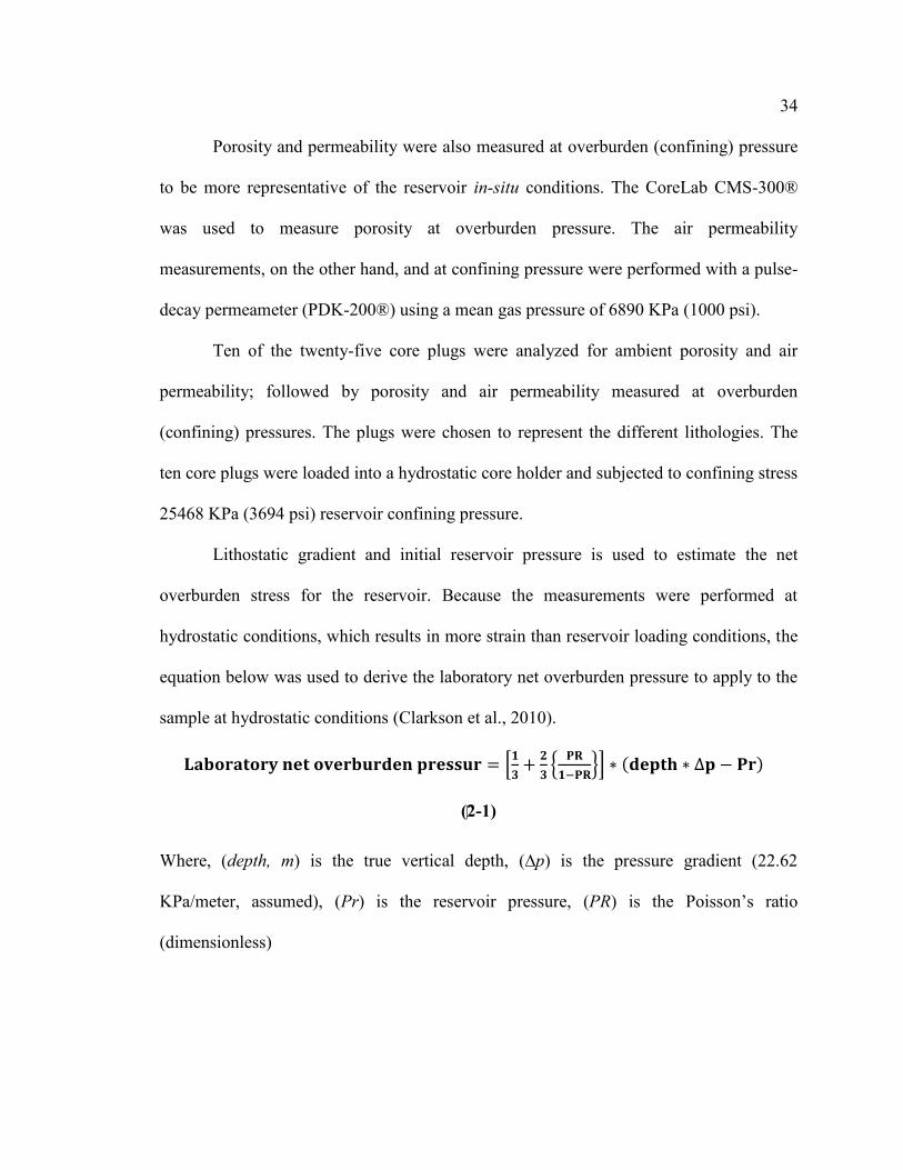
34

Porosity and permeability were also measured at overburden (confining) pressure

to be more representative of the reservoir in-situ conditions. The CoreLab CMS-300®

was used to measure porosity at overburden pressure. The air permeability

measurements, on the other hand, and at confining pressure were performed with a pulse-

decay permeameter (PDK-200®) using a mean gas pressure of 6890 KPa (1000 psi).

Ten of the twenty-five core plugs were analyzed for ambient porosity and air

permeability; followed by porosity and air permeability measured at overburden

(confining) pressures. The plugs were chosen to represent the different lithologies. The

ten core plugs were loaded into a hydrostatic core holder and subjected to confining stress

25468 KPa (3694 psi) reservoir confining pressure.

Lithostatic gradient and initial reservoir pressure is used to estimate the net

overburden stress for the reservoir. Because the measurements were performed at

hydrostatic conditions, which results in more strain than reservoir loading conditions, the

equation below was used to derive the laboratory net overburden pressure to apply to the

sample at hydrostatic conditions (Clarkson et al., 2010).

[

{

}] ( )

(‎2-1)

Where, (depth, m) is the true vertical depth, (∆p) is the pressure gradient (22.62

KPa/meter, assumed), (Pr) is the reservoir pressure, (PR) is the Poisson’s ratio

(dimensionless)

35

Results and Discussion 2.4

Core Description 2.4.1

The Montney Formation in the analyzed wells are highly heterogeneous. It is

characterized by finely inter-bedded very fine-grained sandstone, siltstone and shale.

Understanding the approaches that were applied in order to evaluate such a

heterogeneous reservoir is very important. Integrating the core analysis and petrographic

analysis is useful to quantify and identify the composition of the rock samples.

The selected cores were chosen to assess the lateral and vertical litho-facies

variability in the studied area. Based on the geological observations of both cores, in

general, the MnC is comprised of very fine-grained sandstones and siltstones with a

multiple of inter-laminated siltstones and shale. The siltstone beds in Well 5-14-78-11W6

are thicker than siltstone beds in the Well 13-12-78-11W6. The core analysis and

description of Wells 13-12-78-11W6 and 5-14-78-11W6 are shown in Figures 2.4 and

2.5.

Shale is classified as a type of mud rocks (Potter, 2003). According to this

classification, shale are sediments with >50% terrigenous material of which >50% is less

than 63 microns (0.063 mm or 0.0025 in.). Further, Potter requires the rock to be fissile

and lithified. In this classification, rock with >67% silt are “siltshale”; rocks with >67%

clay are “clayshale” and between these are “mudstone”.

Detailed geological core descriptions were done for the entire core in the studied

wells, but the Montney B (MnB) was not included for further petrophysical analysis in

this research. The core is dominated by horizontally laminated silts and shales, with few

36

physical or biogenic sedimentary structures such as mud drapes, wave and ripple

laminations.

The studied cores show the vertical changes in composition on a millimeter to

centimeter scale. The grain sizes range from shale, siltstone, to a very fine-grained

sandstone. The MnC is characterized by finely-laminated planar and rippled siltstone.

The presence of siltstone/shale in the MnC suggests a low original porosity, which was

further reduced due to the compaction and diagenesis.

Sedimentary structures of thin-laminated very fine grained sandstone and siltstone

include graded beds with interbedded shale. Shale and siltstone are characterized by

planar to irregular laminations with rare mud drapes, wave and ripple laminations, and

horizontal trace fossils within the siltstone Figure 2.6.

Non-planar laminations with inclined bedding or beds disturbed by bioturbation

are observed in some intervals. Sharp to irregular bed contact and the wavy ripple to the

climbing-up structures were also observed in the study cores. Thickness and abundance

of the siltstone beds and laminae are variable along the length of the cores.

The studied shale and siltstones have been interpreted as being deposited by the

turbidity currents at the toe of the slope break where the gravity flows decelerate

(Moslow & Davies, 1997). In Well 13-12-78-11W6, the thicknesses of silt bedding are

variable with the bedding thickness decreasing toward the top of the core. The core is

characterized by planar lamination, ranging from thick at the base to thin at the top. The

silts beds are divided into two units, which are the MnB and the MnC.

The unit MnC representing the upper part of the core is characterized by finely-

laminated silt and shale, with silt beds occurring on the mm scale and separated by shale

37

beds 0.5 cm to 10 cm (2.5 cm in average). These sediments appear to represent as a basin

plain turbidite deposit based on Mutti’s classification (1977), and can be classified as

deposits located further from the channels and fan lobes into an outer fan.

The unit MnB of the lower part of the core is characterized by thickly bedded silts

interbedded with thick shale of 5-15 cm thickness. The average distance between the silt

interbeds is 75 cm. These features appear consistent with the fan-fringe turbidite deposits

as classified by Mutti (1977). These deposits are located on the distal edges of the

turbidite lobes (Freeman, 2011).

This interpretation of the variability between MnB and MnC could be explained

by the gradual movement of a turbidite fan, with facies MnB being more proximal to the

lobe. Unit MnB overlies the thick turbidite deposit of the Glacier Pool supporting this

interpretation. However, more core studies can verify the lateral distribution of the

different facies (Freeman, 2011).

The boundaries and contact between the two units is gradational. Wire-line log

responses in the turbidite deposit in the studied wells are not obvious and it is hard to

recognize that it corresponds to a turbidite. Shale beds in the MnB are thicker than shale

beds in MnC. The thick shale and sandstone intervals in MnB are recognized by the

gamma ray and resistivity responses. The high gamma ray responses of the logs may

suggest the presence of organic matter in the MnB.

Using conventional logging tools, over the unconventional reservoir, which is

characterized by thin siltstone/shales in the Lower Triassic of Montney Formation, will

have large uncertainties because the spatial distributions of the reservoir properties are

heterogeneous at a small scale.

38

Figure ‎2-4: Core interval 2196-2213.22 m in well 13-12-78-11W6, consists of grey to

light grey very fine grained sandstone, siltstone and shale. Siltstone thickness

decreases upward from 4 to 1 cm; with an upward increase in sandstone and

siltstone content.

39

Figure ‎2-5: Core interval 2188-2206 m in well 5-14-78-11W6, consists of finely inter-

bedded sandstone, siltstone and shale. Sandstone and siltstone thickness is variable

throughout the core; with bed thickness ranging from 3 to 20 cm. Thickness of shale

beds is decreasing up-ward from an average of 25 to 10 cm.

Mn

C

40

Figure ‎2-6: (A) Finely laminated planar and rippled siltstones. (B) thin-bedded

siltstone to shaly-siltstone, 3- 15 cm thick, grade upward into climbing ripple

laminations. (C) Planar laminated very fine-grained silty-sandstone to shaly-

siltstone. (D) Fine siltstone and shale laminations. (E) Normally graded turbidite

bed displaying planar laminations, grading upward into climbing ripple

laminations, and capped by silty-shale bed. Siltstone and shale thickness ranges

from 1-3 cm.

A B C

D E

41

Petrographic Analysis 2.4.2

Leyva et al. (2010) presented petrographic rock types for the core in Well 13-12-

78-11W6 and identified the mineral distribution using thin sections (TS). Thin sections

were prepared by impregnating the rock with blue epoxy to highlight the pore space and

the staining with Alizarin red to help distinguish calcite.

The samples have a different texture and framework grain sizes. A petrographic

analysis of the thin sections indicates that the framework grains are comprised of quartz

and carbonate grains. The matrix consists of clay, mica, pyrite and organic matter. Due to

the fine-grained nature of the samples, a detailed mineralogical analysis was impossible

and inaccurate, and thus many of their optical properties were obscured (Freeman, 2011).

Table 2.2 summarized the thin section descriptions. Wire-line logs over core interval and

samples are shown in Figure 2.7.

Table ‎2-2: Summary of texture, grain size and composition from thin sections

(Leyva et al., 2010)

Composition (%)

TS No.

Log Depth

(m)

Avg. Grain Size (µm)

Textural Classification

Sorting Grain Shape

Qz Dol Cal Matrix + OM

Micas Pyrite

1 2199.9 64 Very Fine Sand

Well Sub-angular

40 15 10 28 5 2

2 2202.8 47.5 Coarse silt Moderate-Poor

Sub-angular

44 20 7 28 1 -

3 2207.64 45.8 Coarse silt Moderate-Poor

Sub-angular

40 35 5 14 5 1

4 2208.1 30 Medium Silt Moderate - Poor

Sub-rounded

20 24 35 15 5 1

42

Figure ‎2-7: GR, resistivity and bulk density logs responses over cored interval in

well 13-12-78-11W6. Due to low resolution of conventional wire-line, thin beds

cannot be detected. The blue areas are pores. Pores are irregularly distributed

through the reservoir.

GR2GAPI0 150

DEPTHM

RT1OHMM0.2 20000

RXOZ1OHMM0.2 20000

RHOZ1K/M32000 3000

Montney

Formation

2160

2170

2180

2190

2200

2210

2220

2230

M

n

C

M

n

B

Core

M

n

D

TS 1

TS 2

TS 4

Q (Quartz), D (Dolomite), CC (Calcite Cement), O (Oraganic Matter), Py (Pyrite), SO (Silica Overgrowth), M (Muscovite),

Ø (Porosity)

43

Bulk X-Ray Diffraction (XRD) was performed by Bustin (2009) to determine the

mineral composition of the siltstone and shale Table 2.3. XRD shows that the sandstone,

siltstone and shale consist in order of abundance of silica, dolomite, orthoclase, and

muscovite. The XRD analysis confirms the thin section observations of the studied

samples, but illite was also observed in trace amounts. Three XRD samples were

collected, with two samples collected from the MnC unit; one sample was retrieved from

the MnB unit.

Sample 1 contains the highest percentage of quartz (42%), with less in samples 2

and 3 (30%). The dolomite content increases with depth (sample 3 has greater amount

compared to the other samples). The orthoclase content is similar for Samples 1 and 2

(18.4% and 18.6%, respectively), while it is less for sample 3 (12.6%).

Although only traces of illite (1.5 – 2%) are observed in the samples, the author

believes that the illite content was underestimated due to the difficulties to distinguish

between the illite and the muscovite using the bulk XRD. Some of the volume attributed

to the muscovite is likely illite (Freeman, 2011).

The average of the chemical analysis for potassium within the study core is 12%

for muscovite and 18% for K-feldspar. This indicates that the K-feldspars contribute the

largest proportion to the potassium content of the formation compared to the illite

because the illite occurs in trace amounts.

Microprobe analysis was done by Freeman (2011) to create chemical maps on the

three retrieved samples. The mineral compositions of samples were demonstrated to be

constant across the coarser lamination. The resulting mineralogy for each sample is

shown in Table 2.4.

44

It is noted that the results obtained from the XRD and microprobe provide similar

values for the quartz, dolomite, pyrite, albite and calcite. The orthoclase, illite and

muscovite contents were less similar Figure 2.8. The author has considered the illite

content as it was produced from the XRD. It was very difficult to distinguish between the

muscovite and illite based on the chemical composition. The microprobe work is

discussed in detail by (Freeman, 2011).

Table ‎2-3: XRD analyses for samples of the Well 13-12-78-11W6. Minerals

constitution is by weight %

Core Depth

(m)

Sample Qz %

Dolomite %

Orthoclase %

Muscovite %

Calcite %

Illite %

Pyrite %

Albite

2197.71 1 41.36 20.03 18.4 9.80 0.02 1.64 1.64 3.26 2198.57 2 29.77 21.40 18.64 15.28 0 1.92 1.81 5.08 2207.6 3 (MnB) 30.8 29.84 12.57 9.72 8.5 0.82 2.15 2.69

Table ‎2-4: Microprobe analyses for samples of the Well 13-12-78-11W6 (Freeman,

2011)

Core Depth

(m)

Sample Qz %

Dolomite %

Orthoclase %

Muscovite %

Calcite %

Illite %

Pyrite %

Albite %

2197.71 1 41.93 20.44 7.92 14.60 0.86 9.72 0.87 2.95 2198.57 2 35.88 19.96 10.09 14.61 0.87 13.96 0.95 2.85 2207.6 3 (MnB) 34.87 24.43 7.01 11.90 1.42 9.07 1.11 1.84

45

Figure ‎2-8: Comparison of XRD and Microprobe mineralogy analysis. Microprobe

based on data from Freeman (2011).

32%

23% 20%

16%

0%

2%

2% 5%

XRD 2

Quartz Dolomite

Orthoclase Muscovite

Calcite Illite

Pyrite Albite

43%

21%

19%

10% 0%

2% 2%

3%

XRD 1

Quartz Dolomite


Calcite Illite

Pyrite Albite

31%

31% 13%

10% 9% 1%

2%

3%

XRD 3

Quartz Dolomite


Calcite Illite

Pyrite Albite

42%

20%

8%

15%

1%

10% 1% 3%

M-Probe 1

Quartz Dolomite


Calcite Illite

Pyrite Albite

36%

20%

10%

15%

1%

14% 1% 3%

M-Probe 2

Quartz Dolomite


Calcite Illite

Pyrite Albite

38%

27% 8%

13%

1%

10%

1% 2%

M-Probe 3

Quartz Dolomite


Calcite Illite

Pyrite Albite

46

Routine Core Analysis 2.4.3

Twenty-seven and ninety-two core plugs from the MnC unit were analyzed from

Wells 13-12-78-11W6 and 5-14-78-11W6, respectively. The average porosity and

permeability values from Well 5-14-78-11W6 are higher than the porosity and

permeability values from Well 13-12-78-11W6 due to the lithology.

Fourteen of the permeability measurements are equal or below 0.01 mD in the

Well 13-12-78-11W6. In general, the permeability values are equal or less than 0.1 mD in

the Well 5-14-78-11W6. However, permeability less than 0.01 mD cannot be measured

by the RCA. Thus the data from the RCA has limited the interpretative potential and the

unreliable quantification in low permeability reservoirs. The cross-plot of the routine air

permeability and the porosity for both wells are shown in Figure 2.9.

Satisfactory correlations from the cross-plot of the porosity-permeability cannot

be obtained by using routine core analysis of the two studied cores. For example, there

are identical permeability values on the different porosities or different permeability

value for the identical porosity values. Also, some outliers that are observed in the

characterization of the low permeability regions will have a significant effect on the

fluid-flow prediction that is not well-presented in the correlation.

The inability to find a correlation between the permeability and porosity is

contributed to an insufficient accuracy of the whole core analysis, or there might not be a

relationship due to the resolution of the RCA measurements and a wide variation in

permeability and porosity.

In general, the full-diameter core analysis results represent the average rock

properties over the studied interval. As a result, the whole core analysis has a tendency to

47

ignore the average of the small scale changes in the rock properties that are common in

the heterogeneous MnFM.

Grain densities were measured on the cores using the RCA. Densities varied from

2690 kg/m3 to 2740 kg/m3, with an average of 2706 kg/m3 for Well 13-12-78-11W6.

Grain densities in the Well 5-14-78-11W6 are greater than 2680 kg/m3 but less than 2780

kg/m3, with an average of 2708 kg/m3 Figure 2.10.

48

Figure ‎2-9: Cross-plot of RCA data between air permeability and porosity for the

studied cores showing poor correlation.

0.01

0.1

1

0.02 0.03 0.04 0.05 0.06 0.07 0.08 0.09

Ro

uti

ne

Air

Pe

rmea

bili

ty, m

D

Routine Core Porosity, Fraction

13-12-78-11W6

0.01

0.1

1

0.02 0.03 0.04 0.05 0.06 0.07 0.08 0.09

Ro

uti

ne

Air

Per

mea

bili

ty, m

D

Routine Core Porosity, Fraction

5-14-78-11W6

49

Figure ‎2-10: Comparison between grain density and the porosity for the studied

cores using RCA. Good correlation between grain density and core porosity was

observed.

2670

2690

2710

2730

2750

2770

2790

0.02

0.03

0.04

0.05

0.06

0.07

0.08

0.09

2188 2190 2192 2194 2196 2198 2200 2202 2204 2206

Gra

in D

en

sity

, Kg/

m^3

Ro

uti

nr

Po

rosi

ty, F

ract

ion

Depth, m

5-14-78-11W6

Routine Porosity, Fraction Grain Density, Kg/m^3

2670

2690

2710

2730

2750

2770

2790

0.02

0.03

0.04

0.05

0.06

0.07

0.08

0.09

2195 2197 2199 2201 2203 2205 2207 2209

Gra

in D

en

sity

, Kg/

m^

3

Ro

uti

ne

Po

rosi

ty, F

ract

ion

Depth, m

13-12-78-11W6

Routine Porosity, Fraction Grain Density, Kg/m^3

50

Profile Permeability and Pulse-Decay Permeability Analysis 2.4.4

Profile permeability analysis was utilized successfully for quantifying the fine

scale lamination and heterogeneity. Figure 2.11 shows the lithology, core gamma ray and

the slip-corrected permeability data set for well 13-12-78-11W6 (MnC unit). A change in

the permeability with depth was observed only in the upper part. Permeability decreases

occurred in an interval of 2196 up to 2199 m. At depths of 2199 m to 2209 m,

permeability is repeated in cycles of around 2 m.

The range of permeability is narrow from 0.0008 mD to 0.03 mD. The narrow

range likely reflects the relative narrow range in the grain size and pore throat radius. The

high permeability, however, may indicate the presence of thin high permeable beds. An

arithmetic average was used to estimate the permeability in the current study.

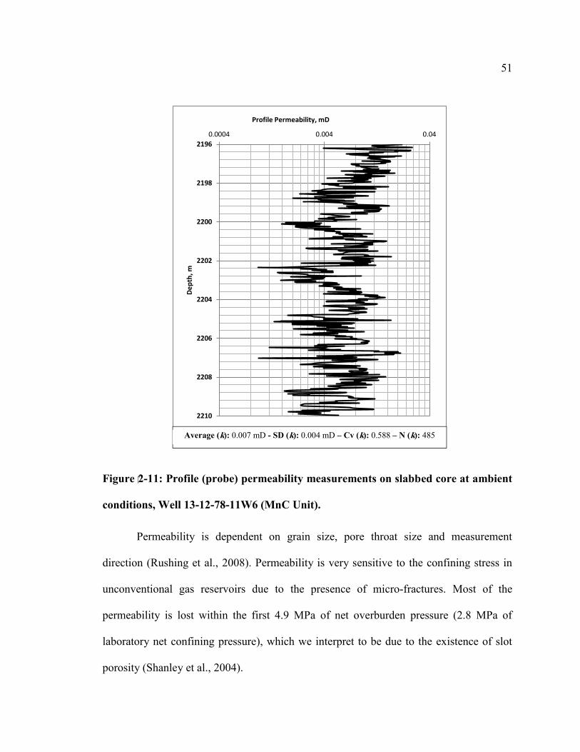
51

Figure ‎2-11: Profile (probe) permeability measurements on slabbed core at ambient

conditions, Well 13-12-78-11W6 (MnC Unit).

Permeability is dependent on grain size, pore throat size and measurement

direction (Rushing et al., 2008). Permeability is very sensitive to the confining stress in

unconventional gas reservoirs due to the presence of micro-fractures. Most of the

permeability is lost within the first 4.9 MPa of net overburden pressure (2.8 MPa of

laboratory net confining pressure), which we interpret to be due to the existence of slot

porosity (Shanley et al., 2004).

2196

2198

2200

2202

2204

2206

2208

2210

0.0004 0.004 0.04

De

pth

, m

Profile Permeability, mD

Average (k): 0.007 mD - SD (k): 0.004 mD – Cv (k): 0.588 – N (k): 485

52

A plot of the pulse-decay permeability measured at two net overburden stresses is

shown in Figure 2.12. It shows that the difference increases with a decrease in

permeability. Based on the ten plugs for measuring porosity and permeability at variable

confining pressures, it is noted that the porosity and permeability strongly decrease with

an increase in net confining pressure Figure 2.12.

Pulse-decay permeability measurements are performed on cylindrical core plugs

and have a range of 0.01 millidarcy to 10 nano-darcies. Porosity measured at an ambient

condition is less than the porosity that was measured at net overburden conditions with

the range of 10-20%. The variable porosity measurements are attributed to lithological

differences.

Figure ‎2-12: Plot of the porosity and permeability from ten core plug at ambient

and various confining (overburden) pressures.

0.0001

0.001

0.01

0.1

1

0.000

0.010

0.020

0.030

0.040

0.050

0.060

0.070

0.080

0.090

0.100

2196 2198 2200 2202 2204 2206 2208 2210 2212 2214

K, m

D

Po

rosi

ty, F

rct.

Depth, m

Well 13-12-78-11W6

Confining Pors., Frct. Ambient Pors., Frct. Confining k, mD

Ambient K, mD Profile K, mD

53

A plot of the pulse-decay permeability measured at two different net overburden

stresses shows the difference increases with a decrease in permeability Figure 2.13. With

knowledge of the dependence of permeability on confining pressure, the probe

permeability can be corrected to in-situ stress conditions Figure 2.14. One sample point

is eliminated due to no difference between permeabilities measured at all condition. The

cause of the stress insensitivity of this sample is uncertain (Clarkson et al., 2010).

The difference between the probe and pulse-decay permeability at overburden

pressure approaches an order of magnitude for most samples. Variation between the

probe and pulse-decay in permeability is observed due to the difference in the condition

of measurement (stress-dependence), and volume of the sample size.

54

Figure ‎2-13: Plot of pulse-decay permeability measured at net ambient pressure

versus pulse-decay permeability measured at reservoir net overburden (confining)

pressure condition.

Figure ‎2-14: Plot of probe (profile) permeability versus pulse decay permeability

measured at net overburden pressure.

0.0001

0.001

0.01

0.0001 0.001 0.01

Pu

lse

-De

cay

K (

Co

nfi

nin

g), m

D

Pulse-Decay K (Ambient), mD

y = 0.3451x0.5988 R² = 0.734

0.00100

0.01000

0.10000

0.0001 0.001 0.01

Pro

file

Pe

rme

abili

ty K

, mD

Pulse-Decay K (Confining), mD

55

Conclusion 2.5

The Montney Formation (MnFM) consists of inter-bedded, very fine-grained

sandstone, siltstone and shale deposited in a low-energy depositional environment. In

other words it is characterized by a non-uniform spatial distribution of the reservoir

properties. The detailed core description plays an important role for identifying the

vertical change in texture, grain size and lithology.

Petrographic and x-ray diffraction analysis was used to define the mineral

composition and their distributions. In addition, it provided the shale volume and type for

the selected samples. Petrographic and the XRD analyses suggest that the MnFM is

composed of dolomite, quartz, calcite with minor amounts of illite and pyrite.

The very fine-grained sandstone-siltstone deposits are separated by thin,

impermeable shale breaks that are not detected by the RCA or wire-line logs. Shale

within the Montney Formation reservoir may influence the fluid flow, depending on the

spatial distribution of the shale.

Routine core analysis is not useful for characterizing such a heterogeneous

reservoir with changes on a millimeter scale. Diagenesis and compaction have altered the

mineralogical composition and dramatically reduced the porosity and permeability.

Profile permeability was useful to define the heterogeneity because of the fine scale of

the measurements. Pulse-decay permeability was used to correct the profile permeability

and porosity to the reservoir stress condition.

56

PETROPHYSICAL CHARACTERIZATION Chapter Three:


Every field is unique in terms of geological and reservoir characteristics, and fluid

properties. Reservoir engineers can attempt to maximize production potential when all of

these factors are considered. Accordingly, engineering and geologic skills, strengthened

by exchange of information, interpretation and judgment, guide our understanding of

reservoir behavior (Briggs et al., 1992).

Rider (2000) noted that most conventional logging tools were developed to

evaluate formations; they perform well over thick beds (> 20 cm) due to variable

resolution. For example, the vertical resolution of the gamma ray log (GR) is 20 cm to

30 cm, Litho-density (LDT) has a resolution of 20 cm to 60 cm depending on the source-

detector spacing, and Deep Induction resistivity (ILD) has a resolution of 2 m.

Rushing et al. (2008) defined the three rock types as follows: (i) Depositional,

which are derived from core-based description and characterized by similarities in

texture, sedimentary structure, and stratigraphic sequences (rocks represent their

properties present at deposition); (ii) Petrographic, rocks described based on pore-scale,

microscopic imaging, texture, composition, clay minerals, and diagenesis; (iii) Hydraulic,

rock that quantified based on the physical flow and storage properties (fluids controlled

by pore geometry, pore and pore throat structure and distribution).

In the Montney Formation (MnFM), each rock type has a distinctive porosity,

permeability, pore throat size, saturation which forms the basis for the dynamic reservoir

properties in this study. Accurate estimates of these properties are required to construct a

dynamic reservoir model.

57

Petrophysical properties are scale-dependent. The difficulty in comparing the

measurements across different scales is compounded by the thickness and heterogeneity

of the various geological elements that are being assessed and the different measurement

conditions.

The MnFM are affected by both the depositional processes and the post-

depositional modification (compaction and diagenesis). Diagenetic alteration creates a

complex permeability distribution of the siltstones in the MnFM. The degree of

permeability distribution, however, is one that must be assessed to predict the

performance of reservoirs in the MnFM.

Using conventional logging tools to quantify the petrophysical properties for the

interlaminated siltstone/shale of the MnFM in the chosen study area will have large

uncertainty because the reservoir properties exhibit heterogeneity at a fine scale. Careful

measurement of the petrophysical properties, core-log calibration and statistical analysis

is required.

It is important to assess the statistical relationships (correlation) of the properties

measured in the MnFM. Statistical procedures (averaging) are often used in up-scaling.

Consequently, the potential for erroneous values is high; several techniques are applied to

reduce these errors in this work.

Methods 3.2

The variability of the geological properties is assessed in this work at various

scales. The scales evaluated include the core-scale (using core description, profile

permeameter and pulse decay permeameter), borehole scale (using wire-line logging

tools) and field scale (using well and field production data). Core measurements and

58

wire-line logs in geological units of the Montney Formation are evaluated for different

particular hydraulic rock type or facies in addition to a depth and well location.

This section covers the methods applied to establish the petrophysical properties

of the studied units and their distribution. These methods include the calibration of the

core analysis to wire-line logs in order to estimate the shale volume, porosity, water

saturation. In addition, an attempt has been made to relate the static properties (porosity)

to the dynamic properties (permeability).

Clay Content from Gamma Ray (GR) and Spectral Gamma Ray (SGR) Logs 3.2.1

The basic GR log records natural radioactivity of formations in a single track in

the API units. Radiation is emitted from naturally-occurring Uranium (U ppm), Thorium

(Th ppm) and Potassium (K %) present in the rock. It can allow differentiation between

the shale and non-shale zones.

To distinguish between the permeable zones by virtue of the fact that the

radioactive elements tend to be concentrated in the shale, which have low permeability,

and are much less concentrated in sands and carbonate, which are generally more

permeable.

The GR log as a shale log was an old principle (Bassiouni, 1994). For example,

the GR logs reflect high readings (deflections) due to the presence of the radioactive

isotopes. In modern interpretation, it is important to understand the mineralogy and

geochemistry causing the radiation. For example, in addition to clays, potassium also is

present in feldspars, which are highly radioactive in sandstone layers.

It is possible to use the GR log to track the clay content. Different kinds of clays

have different effects on tight gas reservoirs, depending on whether they are pore-lining

59

or pore-bridging (Dewan, 1983). The Spectral Gamma Ray log (SGR), however, records

the total GR count from the three emitters (U, Th and K).

Common applications of the SGR log are in the estimation of the clay mineral

volumes (and types). The behavior of the individual radioactive elements in the clay

minerals and clays in general are different based on the ratio of the emitters. In some

rocks it has been established that the thorium-potassium components (without uranium

ratio) are better indicators of clay contents than the total GR activity (Rider, 2000).

Shale affects every logging tool to some degree; numerous methods have been

developed to indicate its presence and to estimate the content of shale. In the studied area,

a preliminary estimates of the volume of shale using the GR log. The gamma ray log is

often used quantitatively, but the values could be erroneous. The volume of shale can be

calculated and related to a shale index (Ish) as follows:

( )

(‎3-1)

Where, ( ) is the gamma ray response in the zone of interest, ( ) is the gamma ray

response in the clean formation, ( ) is the gamma ray response in the shale

Equation 3-1 tends to exaggerate the shale volume (Bassiouni, 1994). Empirical

relationships between Vsh and Ish for different geologic ages and areas have been found to

be more reliable. Historical correlations have been developed by Larionov (1969), Stieber

(1970) and Clavier et al. (1971). The correlations developed by Larionov (1969) for older

rocks (older than Tertiary rocks) were used in current study.

( ) (‎3-2)

60

Computed gamma ray (CGR), results from the subtraction of the uranium

contribution from the SGR. Thorium and potassium content vary for different rock types;

therefore, the CGR is the summation of thorium and potassium sources. This curve

provides an improved method to estimate clay content, free of perturbations by uranium

because uranium is not associated with shale (Bassiouni, 1994).

Potassium and thorium contents vary for different types of clay. The use of (Ish)K

or (Ish)Th alone to determine Vsh could lead to incorrect value (Bassiouni, 1994). The type

as well as the amount of clay encountered in the formations is determined by Th and k

ratio.

If the thorium to potassium ratio is less than four in sandatone and siltstone, the

zone is dominated by feldspars and illite (Rider, 2000). The product index using the

CGR, which represents the contribution of the thorium and potassium, is virtually

independent of the clay type. The potassium-thorium cross-plot is useful for the

recognition of clay minerals and distinction of k-feldspar and mica.

The equation below was used to calculate the shale index more accurately from

the GR log and combined elements (emitters) from the spectral GR log. A complex

quantitative approach to the clay mineral identification has been proposed (Quirien et al.,

1982). They suggested that the clay mineral species, along with the feldspar can be

identified relatively by Th/K ratio.

61

( ) [( ) ( ) ] [( ) ( ) ] (‎3-3)

Where, ( ) is the k and the Th curve readings in the zone of interest, ( )

is the k and Th curve readings in the cleanest zone, ( ) is the k and Th curve

readings in the shale

Porosity Estimation from Density Logs (RHOB) 3.2.2

Density logs are used to estimate the formation’s bulk density. Bulk density is the

overall gross density of the formation, which includes the matrix and the fluid (oil, gas,

water) content in the pores. Quantitatively, the density log is used to calculate porosity.

Mathematically, bulk density and porosity can be expressed respectively by:

( ) (‎3-4)

( )

( ) (‎3-5)

Where, ( ) is the bulk density, kg/m3, ( ) is the porosity (fraction), ( ) is the matrix

density, kg/m3, and ( ) is the fluid density kg/m3

Service companies assume the density measurement is being made on a relatively

homogeneous lithology with the mud filtrate invasion to be at least the depth of

investigation (radial response of the measurement in one or more directions) of the

density porosity tool. Such assumptions are incorrect at studied units because the MnFM

is lithologically heterogeneous (mineral compositions varies with lithology; and it

appears that the zones have a shallow, but variable invasion profile).

The presence of shale complicates the interpretation of the porosity log response

due to the various characteristics of the shale and the different responses of each porosity

tool to the shale content. A standard technique uses the cross plots of log data (using

62

combined density and neutron logs to interpret porosity); a shale point, clean sand line

and shale line are established. The existence of a shale point represents an inconsistency

because 100% shale does not represent 100% clay in the MnFM (only trace amount of

illite was observed).

In addition, flushed zone saturations in this technique are required to remain

constant, which is not possible with the zones associated with clay. As a result, taking the

average of the density and neutron logs does not contribute to the counterbalance of each

other as the clay effect on the neutron log is much higher.

The clay also impacts the sonic log responses. Many assumptions are required to

use sonic logs for the studied unit due to the limited information. As a result, the

uncertainty can be associated with the porosity calculation using the sonic logs. The

density log measurements are therefore used as the primary method for porosity

calculation.

Density porosity is corrected for the shale and gas effects to determine the

effective porosity (Øe) of the shaly-siltstone/sandstone as follows:

(‎3-6)

√( ) = ( ‎3-7)

Where, ( ) is the porosity from density with the shale correction, ( ) is the porosity

from density without the shale correction, ( ) is the shale porosity from density

Statistics and Geo-statistics 3.2.3

Core analysis data from the laboratory was reviewed for quality prior to use for

wire-line log calibration. A newly developed method of statistical analysis for log data

63

was applied to obtain a better definition and calibration of the reservoir properties. The

application of this approach can play a critical role in the exploration and development

decision-making processes for the Montney gas reservoirs.

Univariate description deals with the organization, presentation and summary of

the data set. The variables, permeability and porosity are used frequently in the current

study. One of the useful presentations of data sets is the frequency table and its

corresponding graph, the histogram. Additionally, the important features of most

histograms can be captured in the summary of statistics such as mean, median, standard

deviation, coefficient of variation (Issak & Srivastava, 1989).

The relationships (correlation) between the permeability and porosity present an

approach for the estimation and description of the reservoir properties. In addition, the

estimation tools will be work better if the distribution of data is known. Furthermore, the

correlation coefficient, regression, conditional expectation is a useful way of defining a

non-relationship between two variables (Issak & Srivastava, 1989).

To reduce the uncertainty in the estimation of hydrocarbon-in-place and fluid

contacts in shale gas reservoirs, it is essential to i) integrate the core data and log analysis

to provide a good match between porosity values determined from the core and log

analysis ii) identify statistical distribution of the permeability and porosity, which is

useful for reservoir characterization.

Spatial features of the data set, such as the location, the overall trend, or the

degree of continuity, are often of considerable interest. The study formation is recognized

by variable and large fluctuation in the permeability and porosity values. However, the

64

calculation of a summary statistics within moving interval is used to investigate the

relationship between the permeability and porosity.

The covariance and the correlation coefficient are used to describe the spatial

continuity between variables. The relationship between the covariance for each lag

distance, and the relationship between the correlation coefficient and lag distance are

known as the covariance function and correlation function (correlogram), respectively.

Covariance is a method that can be used was to capture the spatial relationship for the

reservoir properties.

Kelkar & Perez (2002) defined covariance under the first and the second-order

stationarity assumptions. The first order of the stationarity assumes that the expected

value of any variable at location ( )) is equal to the expected value some distance away

at the location ( ), mathematically can be written as:

[ ( )] [ ( )] (‎3-8)

Where, [ ] , is the function of a random variable, [ ( )] is the expected value of a

random variable at , [ ( )] is the expected value of a random variable a lag

distance away

The expected value itself is an arithmetic mean, which assumes that the means of

the variables across the zone of interest are the same. In practice, the means of the

variables over the zone of interest can differ frequently from unit to unit, however, this

assumption may not be possible to apply for the heterogeneous formations such as the

MnFM; therefore, the second option below is used more often.

65

The second stationarity states that any function of any two variables located

distance is independent of the location and is a function only of the distance and direction

between the two locations. The Mathematical covariance can be written as:

[ ( ) ( )] [ ( ) ( )] (‎3-9)

The covariance within the interested zone of the stationarity is a function only of

the distance and direction. The estimated covariance (relationship) of any two variables

for the two points given the distance and direction between these points can be calculated

as:

( )

( )∑ ( ) ( ) ( ) (‎3-10)

Where, ( ) is the arithmetic mean of the sample data

The data collected from the studied wells is one direction (vertically). The

correlation coefficient also used to describe the spatial relationship as the following

equation:

( ) ( )

( ) (‎3-11)

Where, ( ) is the sample variance at distance zero

Permeability-Porosity Relationships 3.2.4

The classic scatter plot of the permeability versus porosity on a semi-log scale has

historically been utilized to aid in identifying the relationship between core permeability

and core porosity (Thomas, 2000). A logical extension for applying the summary

statistics principles is establishing a linear relationship between the two variables.

66

A linear relationship is useful in predicting a value of one variable when the value

of the other variable is known. The simplest type of this relationship is:

(‎3-12)

Nelson (1994) published a paper with a comprehensive discussion of the methods

available at that time. He showed that the most successful models can be characterized by

a linear relationship in the log-log permeability-porosity coordinate system, with the

following generic form:

(‎3-13)

Porosity is generally not dependent upon the grain size, while, the permeability is

very much grain size dependent (Amaefule et al., 1993). The permeability of a rock

depends on its effective porosity; consequently, it is affected by the rock grain size, grain

shape, grain size distribution (sorting), grain packing, and the degree of consolidation and

cementation. The type of clay or cementing material between sand grains also affects

permeability (Tiab & Donaldson, 2004).

In tight rocks, pore structure (pore and pore throat dimensions, geometry, size,

distribution) is a key control on fluid flow and storage properties. Original pore structure

is often modified by diagenesis, which reduce pore throat diameter. As a result, it

increases both tortuosity and disconnected pores (Rushing et al., 2008).

Understanding the stress sensitivity of the porosity and permeability data derived

from the laboratory core samples is critical for establishing the in-situ estimates of these

properties. Porosity and permeability data collected at ambient conditions can be

67

corrected to reflect the in-situ reservoir conditions. Additionally, permeability determined

at various stress conditions can be used to ascertain the permeability variation with depth.

Water Saturation from Resistivity Logs 3.2.5

The resistivity log is a measurement of the formation’s resistivity. Induction tools

measure deep resistivity (Rt) for the virgin formation in wells drilled with oil-based mud.

It is essential to realize that the same porous bed can have a multitude of resistivity

responses, depending on the fluid content.

There is no separation exhibited on the micro-log resistivity log in the studied

wells, possibly due to low permeability. Thus, it was not considered in the study. In

addition, the caliper log is used for the borehole diameter measurement. As a result,

vertical intervals of the studied wells show regular shape and no indication of filter cake

was detected, which indicate the presence of low permeable or non-permeable intervals.

Qualitatively, the resistivity tools are used for recognition of lithologies, taking

into consideration the variables such as compaction, composition and fluid contents. Low

resistivity can be associated with conductive lithologies such as shale or are affected by

the mineral concentration such as pyrite. In contrast, high resistivity can indicate the

presence of hydrocarbon in the formations.

In general, the resistivity increases as the hydrocarbon saturation increases. When

used jointly with other logging tools, the resistivity tool can be used with caution to

correlate the zones with more rapid vertical changes than to lateral changes. Caution is

required for the resistivity response interpretation due to the post-depositional elements

that tend to obliterate the original depositional features.

68

Moreover, distinctive shapes, trends or peaks over the shale zones are related to

the compositional vertical change reflecting the patterns of sedimentation. Finally,

resistivity responses can be used in petrofacies analysis due to their ability for recording

the grain-size variation (Rider, 2000). Consequently, it should be used to evaluate

permeability.

Quantitatively, resistivity with porosities values can be used to estimate the water

saturation (Sw) for the study units. Water saturation is a critical reservoir parameter as it

has a great affect upon effective gas permeability (Kukal et al., 1983) as well as gas-in-

place. Archie (1942) performed experimental studies of clean sandstone formations, and

arrived at the following empirical relationship:

(

) (

) (

) (‎3-14)

Where, ( ) is the saturation exponent (often assumed to equal 2), ( ) is the rock

resistivity, ( ) is the formation resistivity factor, ( ) is the constant (varies with pore

geometry, often taken to be 1), ( ) is the water resistivity, ( ) is the porosity, ( ) is

the cementation factor (varies around 2), ( ) is the observed bulk resistivity

The advantage of this conventional technique is that it is well-established and is

relatively easy to apply. The calculated water saturation value is susceptible to error

because of it requiring a large number of the parameters such as Rw, a, m and n

(Bassiouni, 1994). Errors in the interpretation of the parameters could lead the analyst to

underestimate or overestimate of the water saturation; consequently it affects the

evaluation procedures.

69

Generally, clay minerals affect all well-logging measurements and to some degree

the porosity and water saturation estimations from logs. Shaly-sandstone/siltstone

exhibits a more complex behavior due to the presence of clay. Clays contribute to the

total conductivity of the rock. However, Sw determination in shaly formations still lacks a

satisfactory solution.

In addition to the conventional conductivity associated with the formation water,

there is a conductivity component associated with the clay. The calculated Sw from the

uncorrected resistivity responses could lead to bypassing of the productive zones because

Sw would be overestimated. A variety models currently are used for evaluation of Sw in

shaly formations.

Along with Archie’s saturation equation, the Schlumberger and Simandoux

models (Bassiouni, 1994) were used for calculation of water saturation in the current

study. The Simandoux and Schlumberger models can be used to calculate Sw

independently of the distribution of clay (Dewan, 1983). Simandoux and Schlumberger

models can be stated as the follows:

Simandoux: (

) [√(

)

] (‎3-15)

Schlumberger: √(

)

( )

( )

(‎3-16)

Where, ( ) is the water resistivity in Ohmm, ( ) is shale volume fraction, ( ) is

the shale resistivity in Ohmm, ( ) is the true resistivity in Ohmm, ( ) is the effective

porosity

70

The disadvantage of using the Simandoux saturation equation is that the model

made measurements using one type of clay (montmorillonite) of constant porosity. In

addition, both the Simandoux and Schlumberger models are not included in the formation

factor (F), and it is assumed that Rsh are taken equal to the resistivity of the adjacent

shale beds which is not observed in the studied cores. However, an attempt has been

made to calculate the Sw by using different models compared to Sw that calculated from

the routine Lab-Core analysis.

Results and Discussion 3.3

Clay Type and Volume 3.3.1

The studied core at 13-12-78-11W6 showed that not all shale zones are

radioactive, and in many intervals showed that siltstone has a high radioactivity element.

The high readings from 2214 m to 2216 m are likely reflecting the associated detrital

minerals such as feldspars and micas with shale. The source of potassium in the studied

succession may be was due to presence of K-feldspar (Orthoclase).

The bulk uranium distribution over the core interval is irregular in this well and

behaves as an independent constituent. The uranium concentration is very low, generally

less than 4 part per million (ppm). This result suggests that the Montney Formation in the

studied well has low organic matter. In contrast, the thorium concentrations are 6-10 ppm

Figure 3.1. The trend of thorium is the main radioactive element, and consequently

influences the trend of the GR response.

The interpretation of the shaly-sandstone log data has long been a challenging

problem. Shale can be distributed in sandstone/siltstone reservoirs in three possible ways

and forms: laminated, structural, and dispersed Figure 3.2. Each form can affect the

71

amount of rock porosity by creating a layer of closely bound surface water on the shale

particle. The laminae affect the porosity and vertical permeability. Structural clay is the

clay deposited as an integral part of the matrix, but it does not affect the porosity.

Dispersed clay occurs in the pores and can reduce the permeability of the formation

(Dewan, 1983).

72

Figure ‎3-1: GR & SGR logging responses over core interval, well 13-12-78-11W6

Figure ‎3-2: Clay distribution modes (From Dewan, 1983)

0

2

4

6

8

10

12

0

20

40

60

80

100

120

140

2194 2196 2198 2200 2202 2204 2206 2208 2210 2212 2214 2216 2218

Rad

io-a

ctiv

e e

lem

en

ts, p

pm

GR

, AP

I

GR, API Ur, ppm Th/k, ppm K, % Th, ppm

MnB MnC

73

The presences of clay minerals were detected by using the SGR analysis. The

Schlumberger chart of the potassium-thorium cross-plot; and their concentrations were

used as the best indicator for shale content and a shale volume indicator (Bassiouni,

1994). The lines that radiate from the origin of the plot have gradients that match with

values of the Th/K ratio. The ratio is a relative measure of potassium richness as related

to thorium.

The cross-plot was used cautiously because the clay minerals show wide

variability in the composition. Th/K ratio (concentrations) plot from the SGR within the

studied interval indicates that there is a contribution from the illite clay mineral. Illite has

a higher potassium ration than the mixed-layer clays or smectite, while kaolinite has little

to none. Generalized fields of expectations of the mineral responses on a thorium-

potassium cross-plot are shown in Figure 3.3.

The studied succession consists of fine to coarse-grained siltstone. Consequently,

identifying the clay as opposed to non-clay radioactive elements is important. From a

combination of petrographic analysis and the XRD work analysis, the studied sequence

was characterized as a mix of carbonate-siliclastic deposits with trace amounts of illite

clay (Leyva et al., 2010; Freeman, 2011).

The illite percentage was estimated from the XRD analyses, and constitutes 2%.

Bulk XRD analysis cannot differentiate muscovite and illite. It is likely that the bulk of

muscovite and illite as determined from the XRD is actually illite (Freeman, 2011). As a

result, the illite amount should be even more due to that there was not a lot of muscovite

evident in the thin section. Additionally, the samples were collected from clean siltstone

which were expected to have low amount of illite.

74

Figure ‎3-3: Thorium-potassium cross-plot of Montney units from well 13-12-78-

11W6 in western-central Alberta. The cluster of points is interpreted as illite.

0

2

4

6

8

10

0 2 4 6 8 10

75

Illite clay contains the greatest amount of potassium; it deposits as a continuous

linings on grain surfaces and tends to grow outward from the grain surface into the pore

space. As a result, the clay can drastically reduce the permeability and resistivity, and its

presence can mask gas indication (Fertl, 1987).

Over siltstone beds within the cored interval, the GR and thorium responses show

a low reading, whereas, the GR and thorium log responses over the shale intervals show

high responses values. The Thomas and Stieber (1975) methodology is applied to rock-

core measurements in order to diagnose the type of shale distribution across the MnC

unit. The cross plot indicates that structural and laminated shale are dominated for the

MnC Figure 3.4.

Figure ‎3-4: Thomas-Stieber cross-plot over core interval using well-logs data. The

cross-plot indicates that structural and laminated shale are dominant type of

shale/clay distribution.

0

2

4

6

8

10

12

0 10 20 30 40 50 60 70 80 90 100

De

nsi

ty P

oro

sity

, %

Volume of Shale Concentration, %

Core Interval for MnC

Structural

Laminated Dispersed

76

Porosity Evaluation 3.3.2

Core analysis indicates that the grain densities vary from 2.69 gm/cm3 up to

2.74 gm/cm3 of well of 13-12-78-11W6. The density range varies from 2.68 gm/cm3 up

to 2.78 gm/cm3 in the well of 5-14-78-11W6. These variations in matrix density can

cause significant errors in the porosity calculation by assuming a static matrix density.

Density porosity, even after being adjusted for variable lithology showed that the

porosities from the density log is either too high or too low compared to core porosities in

the studied well 13-12-78-11W6. The cause of high porosity from density due that the

density tool is detecting gas close to the borehole (the gas is not deeply invaded).

Consequently, the pore fluid density is not always constant.

Bulk XRD analysis shows that the studied units contain a very small clay amount

with an average density of 2.75 gm/cm3. The other minerals, dolomite, calcite and pyrite

minerals have density average of 2.84 gm/cm3, 2.71 gm/cm3 and 5 gm/cm3 respectively

and will increase the density of the matrix.

Caution was used in applying the results of computer analyses of well logs

provided by different service companies of the studied wells. In comparing the results of

RHOB measurements for the studied wells, it was noted that the average bulk density for

well 16-12-78-11W6 was less than the average of bulk density of Wells 13-12-78-11W6

and 5-14-78-11W6 by 20 kg/m3.

Wells 13-12-78-11W6 and 5-14-78-11W6 had core data and to which the logs

were correlated. These are considered as references wells. A cumulative frequency

distribution has been made to verify the difference in the density profiles for the various

wells.

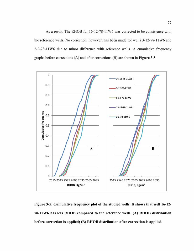
77

As a result, The RHOB for 16-12-78-11W6 was corrected to be consistence with

the reference wells. No correction, however, has been made for wells 3-12-78-11W6 and

2-2-78-11W6 due to minor difference with reference wells. A cumulative frequency

graphs before corrections (A) and after corrections (B) are shown in Figure 3.5.

Figure ‎3-5: Cumulative frequency plot of the studied wells. It shows that well 16-12-

78-11W6 has less RHOB compared to the reference wells. (A) RHOB distribution

before correction is applied; (B) RHOB distribution after correction is applied.

0

0.1

0.2

0.3

0.4

0.5

0.6

0.7

0.8

0.9

1

2515 2545 2575 2605 2635 2665 2695

Cu

mu

lati

ve F

req

ue

ncy

RHOB, Kg/m3

2515 2545 2575 2605 2635 2665 2695

RHOB, Kg/m3

16-12-78-11W6

3-12-78-11W6

5-14-78-11W6

13-12-78-11W6

2-2-78-11W6

A B

78

The evaluation of shaly formations has long been a difficult task, but an accurate

porosity determination is necessary for effective log interpretation. Porosity estimation in

the studied unit is even more difficult because of the variable mineralogy causing the

matrix density to change over the evaluated interval.

Although the thin section analysis is probably not accurate, the thin section

analysis and minerals distribution in percentage have been calculated in order to

determine the apparent matrix density (ρmaa). Using a graphical Schlumberger chart to

find the matrix density, the estimated average of the apparent matrix from the

petrographic analysis was 2.72 gm/cm3 Figure 3.6.

The result from the XRD however is more accurate. The mineralogical

compositions mainly are quartz and dolomite, which represent around 50-60% of the

sample weight. The microprobe was used to examine the textural relationships between

grains, and identify any unknown minerals. The resulting mineralogy from the

microprobe and the XRD analysis and the calculation of the minerals distribution is

summarized in Table 3.1.

Table ‎3-1: Minerals Distribution by thin section, microprobe and XRD analysis

Minerals Distribution (Thin Section), % Minerals Distribution (XRD & Microprobe), %

TS

No.

Log

Depth

(m)

Qz

%

Dol

%

Cal

%

ρmaa

gm/cm3

Core

Depth

(m)

Qz

%

Dol % Calc.

%

ρmaa

gm/cm3

1 2199.9 61.53 23.07 15.38 2.7 2197.71 67.3 32.26 0.03 2.71

2 2202.8 61.97 28.16 9.85 2.71 2198.57 58.17 41.8 0 2.74

3 2207.64 50 43.75 6.25 2.76 2207.6 45.0 43.6 12.44 2.76

4 2208.1 25.31 30.37 44.30 2.74

79

Figure ‎3-6: ρmaa vs Umaa identification plot. Rock mineralogy and matrix were

identified by the position of the data point relative to the points on the plot. (Black)

– Thin section; (Red) – Microprobe and XRD.

2.2

2.3

2.4

2.5

2.6

2.7

2.8

2.9

3

3.1 2 4 6 8 10 12 14 16

U maa maa, , Apparent matrix volumetric photoelectric factor

ρmaa, gm/cc

80

Utilizing “litho-porosity cross-plots”, both porosity and matrix characteristics can

be defined using dual-mineral analysis. Photoelectric absorption indexes (Pe) were used

with density logs to enhance the analysis. By itself the photoelectric absorption index (Pe)

curve is a good matrix indicator in units of barn/electron (Gardner & Dumanior, 1980).

Also, it can be used as the matrix indicator with the corresponding density log

value (Rider, 2000). The averages reading of the Pe logs are slightly over 3 b/e

(barn/electron), which is close to a dolomite response for all of the studied wells. The

average Pe was 3.34 b/e and 3.14 b/e for the Wells 13-12-78-11W6 and 5-14-78-11W6,

respectively Figure 3.7.

Dual-mineral analysis was used to evaluate the density of the matrix for the

studied Well 13-12-78-11W6. The two-minerals, quartz and dolomite, are assumed as the

matrix based on the core analysis, thin sections, microprobe and the XRD results. The

dual-mineral equation for either ρb-ØN combination to readout Øta and ρmaa, or the ρb-Pe

combination to determine the proportions of the minerals in the matrix are given in

Figure 3.8.

The result from the graph shows that both values to obtain the porosity Øta, are

equal or are of close value by using ρb-ØN combination and ρb-Pe combination, which

reflect the choice of minerals, is correct. Moreover, when Øta (ρb-ØN) is less than Øta (ρb-

Pe) in some intervals in the studied well is confirming the presence of gas. In general, the

inputs are ρb (measured bulk density), and Pe, whereas, the outputs are apparent to the

total porosity (Øta) and the apparent matrix density (ρmaa).

Table 3.2 summarizes the results of the porosity and matrix calculations for the

studied well. The average matrix densities of 2690.7 kg/m3 and 2692.7 Kg/m3 were used

81

for the wells 13-12-78-11W6 and 5-14-78-11W6, respectively. The average densities are

used in the porosity calculation for un-cored interval. The calculated porosity from the

service company in the Table 3.2 was calculated based on limestone density.

The Øta is obtained from ρb-Pe combined with the following equations:

(‎3-17)

(‎3-18)

(‎3-19)

(‎3-20)

( ) (‎3-21)

Where (ρb) is the measured bulk density, (Pe) is the measured effective photoelectric

absorption cross section index, (ρf) is the fluid density, (Uf) is the fluid volumetric cross

section, (ρe) is the electron density index, (ρ1,2) is the density of minerals “1,2”, (U1,2) is

the volumetric cross section of minerals “1,2”, (V 1,2) is the bulk volume of minerals

82

Figure ‎3-7: LDT & RHOB responses over the studied cores. As the LDT increases,

RHOB increases.

2.8

2.9

3

3.1

3.2

3.3

3.4

3.5

2520

2540

2560

2580

2600

2620

2640

2660

2188 2190 2192 2194 2196 2198 2200 2202 2204 2206

Pe

, B/E

RH

OB

, Kg/

m^3

Depth, m

5-14-78-11W6

RHOB, Kg/m^3 Pe, barns/electron

2.5

2.7

2.9

3.1

3.3

3.5

3.7

3.9

2520

2540

2560

2580

2600

2620

2640

2660

2680

2700

2196 2198 2200 2202 2204 2206 2208 2210 2212 2214 2216 2218

Pe

, B/E

RH

OB

, Kg/

m^

3

Depth, m

13-12-78-11W6

RHOB, Kg/m^3 Pe, B/E

83

Figure ‎3-8: Nomograph for determination of matrix, porosity and the lithology

proportions (from Gardner & Dumanoir, 1980). Average of Øta was 0.069 (red dot)

by using average values of ρb & ØN Lst, which are 2.57 gm/cm3 & 0.067, respectively.

Average of Øta was 0.077 (blue dot) by using average values of ρb & Pe, which are

2.57 gm/cm3 & 3.28 barn/electron, respectively.

84

Table ‎3-2: Summary of the values to identify the matrix, and to correct the porosity

for unit of MnC using dual-mineral analysis chart for the core, well 13-12-78-11W6

Depth (m)

Nphi-Lst

Pe (b/e)

ρb (Kg/m3)

Øta % ( ρb- ØN)

Øta % ( ρb-Pe)

Ρmaa (kg/m3)

D:Qz Calculated Ø (Frct)

Corrected Ø (Frct)

2195.93-2198.98 0.068 3.29 2571.96 7 7.5 2700 30:70 0.047 0.086

2198.98-2200.04 0.069 3.38 2553.17 8 8 2690 25:75 0.058 0.080

2200.04-2201.57 0.067 3.15 2583.18 7 7 2700 30:70 0.040 0.086

2201-57-2203.55 0.067 3.16 2595.33 6.5 6 2710 40:60 0.033 0.073

2203.55-2205.53 0.065 3.25 2576.91 6.5 7 2680 25:75 0.044 0.071

2205.53-2207.05 0.071 3.43 2570.31 7 7 2680 25:75 0.048 0.065

2207.05-2207.97 0.064 3.29 2566.12 6.5 7 2675 30:70 0.050 0.069

2207.97-2209.06 0.076 3.41 2588.44 7 5 2700 40:60 0.037 0.069

The density porosity log was compared to routine core porosity. The trend of

grain density derived from logs was comparable with the grain density from the core

analysis Figure 3.9. A depth-shift of 3.08 m was required to match the driller core depth

to the log depth for Well 13-12-78-11W6. No depth shift however was made for Well 5-

14-78-11W6.

A correlation after the depth-shift of the density porosity ot the core porosity; and

the sonic porosity to the core porosity is shown for both units of the studied wells in

Figure 3.10. To calculate the sonic porosity (Assumed transit time for matrix velocity

(∆mtx= 180 Sec/m), and fluid transit time (∆fl= 620 Sec/m). For both wells, the

correlation of the density porosity with core porosity is slightly better than the correlation

of the sonic porosity with core porosity. The similarity of the density and sonic porosities

values may indicate that no micro-fracture is presented in the cores interval.

85

Figure ‎3-9: Core analysis indicates that the grain densities average of 2696.1 kg/m3

for well 13-12-78-11W6. The average of the grain density for the well 5-14-78-11W6

is 2692.7 kg/ m3.

2640

2650

2660

2670

2680

2690

2700

2710

2720

2730

2740

2520

2540

2560

2580

2600

2620

2640

2660

2186 2188 2190 2192 2194 2196 2198 2200 2202 2204 2206

Gra

in D

en

sity

, Lo

g

Gra

in D

en

sity

, Co

re

Depth, m

5-14-78-11W6

Grain Density (Core), Kg/m3 Grain Density (Log), Kg/m3

2670

2680

2690

2700

2710

2720

2730

2740

2670

2680

2690

2700

2710

2720

2730

2740

2750

2198 2200 2202 2204 2206 2208 2210 2212

Gra

in D

en

sity

(Lo

g), K

g/m

3

Gra

in D

en

sity

(C

ore

), K

g/m

3

13-12-78-11W6

Grain Density (Core), kg/m3 Grain Density (Log), kg/m3

86

Figure ‎3-10: Correlation of the 27 sample points of core plug samples versus density

and sonic porosity for unit MnC.

R² = 0.15

R² = 0.06

0.02

0.03

0.04

0.05

0.06

0.07

0.08

0.09

0.02 0.03 0.04 0.05 0.06 0.07 0.08 0.09

Co

re P

oro

sity

, Frc

t.

Log Porosity, Frct.

Correlation of Core Porosity vs Logs Porosity, WELL 5-14-78-11W6

R² = 0.46

R² = 0.41

0.01

0.02

0.03

0.04

0.05

0.06

0.07

0.08

0.09

0.1

0.02 0.03 0.04 0.05 0.06 0.07 0.08 0.09 0.1

Co

re P

oro

sity

, Frc

t.

Logs Porosity, Frct.

Correlation of Core Porosity vs Logs Porosity, well 13-12-78-11W6

Density Porosity Sonic Porosity

87

Comparison of Logs to Profile Permeability 3.3.3

Profile permeability measurements of slabbed core were done by LabCore. The

profile measurements were overburden corrected to in-situ stress condition by using

pulse-decay permeability. The relationship between pulse-decay permeability for 10 core

plugs to the corresponding profile permeability was derived. Profile permeability data

then corrected to in-situ stress condition. Detailed of this methodology can be found in

(Clarkson et al., 2010).

The corrected profile permeability was then correlated to the GR and density

porosity logs for the MnC unit. Because of the differences in the scale of the profile

permeability measurements and the logs, the profile permeabilities compared to the core

GR and wire-line GR. The GR, however, captured well the profile permeability variation

at some depths.

As the GR and bulk density decreases, the permeability increases in most of the

core interval. The permeability trend decreases from the top of the core to the depth point

of 2199 m. The relationship between the GR and permeability below 2199 m may

suggest a cyclic deposition of turbidite in meters scale. It also may suggest that the

lithological and composition is controlling the permeability Figure 3.11.

88

Figure ‎3-11: Permeability increases when GR decreases. Interval of 2204.5-2207.5

m, uncertainties are associated of the relationship between GR and permeability in

some depths.

2200 2500

Core Density,Kg/m^3

2196

2196.5

2197

2197.5

2198

2198.5

2199

2199.5

2200

2200.5

2201

2201.5

2202

2202.5

2203

2203.5

2204

2204.5

2205

2205.5

2206

2206.5

2207

2207.5

2208

2208.5

2209

50 100 150D

ep

th, m

Core GR, API

Wire-line GR, API

0.0008 0.08

Probe k, mD

89

The density porosity relationship with the profile permeability was analyzed next.

The profile permeability were averaged over seven points and correlated to the porosity

from the density log. The covariance function and correlation function (correlogram) are

used to describe the relation between the neighboring values of the well Figure 3.12.

For the covariance function and correlation function, ninety two samples of the

density porosity and corresponding permeability were calculated using an Excel program.

In the most intervals, the density porosity has a good correlation with the permeability.

Further, the covariance function and correlogram for the variables also have been given a

good indication of how both are varied as a function of the separation distance. The

relationship between the variables based on the covariance function and correlogram,

however, is used to divide the interval into the different groups. Each group is

characterized by the average porosity and permeability values.

90

Figure ‎3-12: Spatial relationship between density porosity and permeability

(covariance & correlation coefficient), well 13-12-78-11W6.

-0.6

-0.4

-0.2

0

0.2

0.4

0.6

0.8

1

1.2

-0.8

-0.6

-0.4

-0.2

0

0.2

0.4

0.6

0.8

1

0 1 2 3 4 5 6 7 8 9

c (h

) k

c (h

) Ø

Lag Distance, m

Covariance for porosity and permeability data

Dpors. K

-3E-07-2E-07-1E-0700.00000010.00000020.00000030.00000040.00000050.00000060.00000070.0000008

-0.0003

-0.0002

-0.0001

0

0.0001

0.0002

0.0003

0.0004

0 1 2 3 4 5 6 7 8 9

r (h

) k

r (h

) Ø

Lag Distance, m

Correlation Coefficient for porosity and permeability data

Density Porosity Permeability

91

Due to the good quality and quantity of data collected for the 13-12-78-11W6

core, a comprehensive correlation is made to verify the values and trends of the reservoir

properties. A comparable response between the core porosity and density porosity is

noted. Also, a similar trend was observed between the bulk density obtained from the

core measurement and the bulk density from logs Figure 3.13.

The porosity estimates from the logs are compared to profile permeability after

the latter was averaged (7 point average) to attempt to match the depth of the resolution

of the porosity logs. The density porosity trends generally match profile permeability

values after averaging for the 13-12-78-11W6 core Figure 3.14.

Results from the correlation between the core porosity and density porosity for the

studied cores of Wells 13-12-78-11W6 and 5-14-78-11W6 are shown in Figure 3.15. The

measured points, in general were divided to split evenly for both studied cores. At some

depth points, the porosity from the density log is higher than the core porosity. The high

density porosity is due to several reasons: the detection of gas close to the borehole; the

assumption that pore fluid density is equal to 1.1 gm/cc; clay effect. The fluid density is

assumed based on the data obtained from the neighbor areas. Also, the lithology

cementation, diagenesis and compaction decrease the core porosity.

In contrast, at other depth points, the core porosity was higher compared to the

density porosity. The high core porosity is due to reverse effects for the mentioned

reasons (above paragraph); condition of core lab measurements. The core porosity is

measured under a lab condition, while, the density porosity was measured in the in-situ

environment condition. In general, the averages of the variation between both the

porosity measurements were acceptable within a range of 0.5 to 1 porosity unit.

92

Figure ‎3-13: Comparison between density logs and log-derived porosity with routine

core measurements (grain density, porosity and permeability), well 13-12-78-11W6.

(A) Density log responses with core density, and (B) log porosity with core porosity

and permeability.

0.01

0.10

1.00

2.46

2.48

2.5

2.52

2.54

2.56

2.58

2.6

2.62

2.64

2198 2200 2202 2204 2206 2208 2210 2212 2214

Pe

rme

abili

ty,

mD

Gra

in D

en

sity

, gm

/cc

Depth, m

A

Core Density, Frct. Density Log, Frct. k, mD

0.000

0.020

0.040

0.060

0.080

0.100

0.120

2198 2200 2202 2204 2206 2208 2210 2212 2214

Po

rosi

ty, F

rct

& P

erm

eab

ility

, mD

Depth, m

B

Core Ø, Frct. k, mD Log Ø, Frct.

93

Figure ‎3-14: Comparison of density porosity with profile (probe) permeability.

Figure ‎3-15: Cross-plot of core porosity versus density porosity.

R² = 0.4643

0.01

0.03

0.05

0.07

0.09

0.11

0.02 0.04 0.06 0.08 0.1

De

nsi

ty P

oro

sity

, Fra

ctio

n

Core Porosity, Fraction

13-12-78-11W6

R² = 0.2795

0.01

0.03

0.05

0.07

0.09

0.02 0.04 0.06 0.08

De

nsi

ty P

oro

sity

, Fra

ctio

n

Core Porosity, Fraction

5-14-78-11W6

0.002

0.02

0.2

0

0.02

0.04

0.06

0.08

0.1

0.12

2198 2200 2202 2204 2206 2208 2210 2212 2214

Pe

rme

abili

ty,

mD

De

nsi

ty P

oro

sity

, Fra

ctio

n

Depth, m

13-12-78-11W6

Density Porosity, Fraction Probe Permeability (Liquid), mD

94

A cross-plot between a 7-point average probe (profile) permeability and corrected

porosity from the density log is showed in Figure 3.16. An acceptable correlation

between the effective porosity and correction profile permeability was obtained. The

following equation was used to fit the data:

( ) (‎3-22)

Where, (k) is the profile permeability, ( ) is the density porosity

The cross-plot shows that the permeability decreases when the density porosity

decrease. Based on the spatial relationship between the porosity and permeability; and

core analysis, the density porosity was used to predict the permeability value for the non-

cored interval of units MnC and MnD in the studied wells.

In addition, these measurements could then be related to the different sub-units

(petrofacies) defined on the core and on the conventional logs. A petrofacies are defined

by Porras et al. (1999) as a rock has a similar pore throat radius and fluid flow

characteristics. Common definition for the petrofacies is to correlate the petrophysical

rock type, pore structure to the physical rock properties such as porosity and permeability

(Rushing et al., 2008).

Preliminary results show a different sub-unit basis on the cross-plot relationship

between the porosity and permeability. A cross-plot of the permeability with the effective

density porosity data is shown in Figure 3.16. The permeability-porosity cross-plot for

the 27 samples of the studied core from Well 13-12-78-11W6 segregates the reservoir to

distinct sub-units.

95

Figure ‎3-16: Log-derived porosity versus permeability at reservoir net overburden

pressure (NOB) for the core measured samples (27 samples), well 13-12-78-11W6.

Statistics for porosity and permeability distribution 3.3.4

Statistics are applied to provide a better understanding of the sample data.

Understanding the characteristics of the information allows us to use it more

productively. The frequency distribution and the plot relative frequencies as well as the

cumulative relative class frequencies as a function of the variable values is one of the

ways to analyze the sample data.

In defining the frequency distribution, we assume a discrete distribution for a

variable. We do not distinguish among the values within the classes; all values are treated

the same. The advantage is that the sample can be characterized with fewer parameters.

y = 0.0697x1.3359 R² = 0.48

0.0001

0.001

0.01

0.02 0.03 0.04 0.05 0.06 0.07 0.08 0.09 0.1

Pe

rme

abili

ty,

mD

Density Porosity, Fraction

Sub-units (Petrofacies)

96

The cumulative relative-frequency diagram also shows the probability of certain porosity

values.

In the studied units, we can conclude that 35 % of the porosity (fraction unit) falls

between 0.04 and 0.06. The cumulative relative histogram plot Figure 3.17 shows that

63% of the porosity values are less than 0.06. On the basis of these permeability and

porosity data, the well was placed in a good part of the reservoir.

The porosity histogram shows a reasonably symmetric distribution. A range of

0.04 to 0.06 porosity peak, another peak of frequency appears at porosity values of 0.06

and 0.08. This may indicate a mixing of the porosity distribution from three different

geological units. Although some units are hard to distinguish from each other, many units

are separated by continuous fine to coarse grain siltstones.

Figure ‎3-17: Relative frequency (A), and cumulative frequency of the density

porosity for the core interval (B). 63% of the porosity values are less than 0.06.

0

0.1

0.2

0.3

0.4

0.5

0.6

0.7

0.8

0.9

1

0.02-0.04 0.04-0.06 0.06-0.08 0.08-0.1

Fre

qu

en

cy

Porosity, Fraction

B

0

5

10

15

20

25

30

35

40

0.02-0.04 0.04-0.06 0.06-0.08 0.08-0.1

Fre

qu

en

cy

Porosity, Fraction

A

97

The permeability distribution in the studied Well 13-12-78-11W6 is skewed

positively Figure 3.18. Although the permeability values range from 0.0003 mD to 0.006

mD, the majority of the values are at the lower end of the region. This type of histogram

is not useful for characterizing a sample because the values are clustered at one end.

One way to overcome this problem is to transform the sample data (log

transform). The log k distribution is much more symmetric than the permeability

distribution Figure 3.19. As a result, the log k and porosity histogram are similar. Both

show the similar trends with three peaks in the histogram plots, one of which is at the

higher end of the values.

For validation, the data set divided into several classes and considers the number

of values falling within each class (generation conditional distribution of permeability for

a given porosity value). Although the number of permeability values in each histogram

are rather limited, a trend is clearly evident. Low porosity values are associated with low

permeability values Figure 3.20.

98

Figure ‎3-18: Histogram of permeability data (A), and a cumulative frequency of

permeability (B) for the well 13-12-78-11W6 core.

Figure ‎3-19: Effect of log transform on permeability histogram (A), and a

cumulative frequency of log permeability (B).

0

0.2

0.4

0.6

0.8

1

1.2

Fre

qu

en

cy

Permeability, mD

B

0

5

10

15

20

25Fr

eq

ue

ncy

Permeability, mD

A

0

5

10

15

20

25

30

Fre

qu

en

cy

Log k, mD

A

0

1020

30

40

50

6070

80

90

100

Fre

qu

en

cy

Log k, mD

B

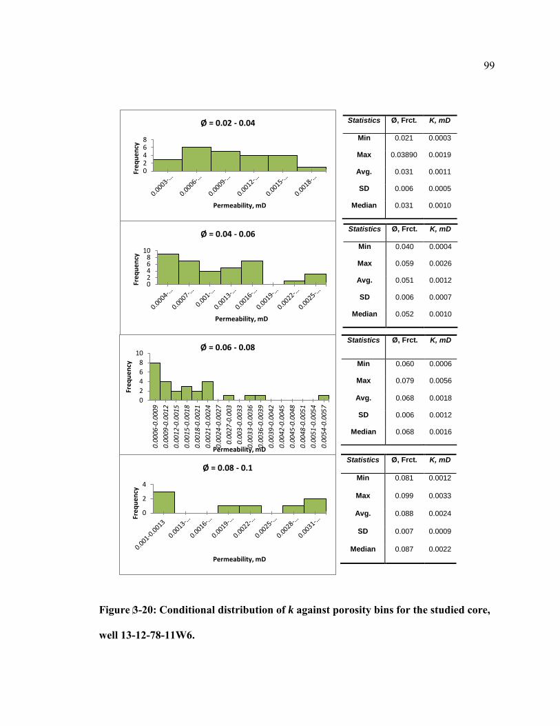
99

Figure ‎3-20: Conditional distribution of k against porosity bins for the studied core,

well 13-12-78-11W6.

Statistics Ø, Frct. K, mD

Min 0.021 0.0003

Max 0.03890 0.0019

Avg. 0.031 0.0011

SD 0.006 0.0005

Median 0.031 0.0010


Min 0.040 0.0004

Max 0.059 0.0026

Avg. 0.051 0.0012

SD 0.006 0.0007

Median 0.052 0.0010


Min 0.060 0.0006

Max 0.079 0.0056

Avg. 0.068 0.0018

SD 0.006 0.0012

Median 0.068 0.0016


Min 0.081 0.0012

Max 0.099 0.0033

Avg. 0.088 0.0024

SD 0.007 0.0009

Median 0.087 0.0022

02468

Fre

qu

en

cy

Permeability, mD

Ø = 0.02 - 0.04

02468

10

Fre

qu

en

cy

Permeability, mD

Ø = 0.04 - 0.06

0

2

4

6

8

10

0.0

00

6-0

.000

9

0.0

00

9-0

.001

2

0.0

01

2-0

.001

5

0.0

01

5-0

.001

8

0.0

01

8-0

.002

1

0.0

02

1-0

.002

4

0.0

02

4-0

.002

7

0.0

02

7-0

.003

0.0

03

-0.0

033

0.0

03

3-0

.003

6

0.0

03

6-0

.003

9

0.0

03

9-0

.004

2

0.0

04

2-0

.004

5

0.0

04

5-0

.004

8

0.0

04

8-0

.005

1

0.0

05

1-0

.005

4

0.0

05

4-0

.005

7

Fre

qu

en

cy

Permeability, mD

Ø = 0.06 - 0.08

0

2

4

Fre

qu

en

cy

Permeability, mD

Ø = 0.08 - 0.1

100

Water Saturation 3.3.5

Qualitatively, the invaded zone resistivity (Rxo) reflects the high resistivity

because an oil base mud was used for drilling the studied Well 13-12-78-11W6. The

Induction device measurement (Rt) shows similar responses. In general, consistent trends

between all three logs were observed.

Based on the XRD analysis and SGR responses, the illite contribution was

determined with a lower percentage. Archie’s model is used for the calculation Sw due to

non-presence of clay and the uncertainty of using shale parameters. In order to determine

the cementation factor (m) and saturation exponent (n) for calculating Sw in the study

area, plots of Sw from core measurements versus Sw obtained from Archie’s equation.

The Schlumberger and Simandoux models are used, and a better-fit between the

core-based and log-based measurements for Sw were obtained. As expected, the average

of the water saturation values from the core closer to the water saturation values from

logs by using Archie’s equation rather than the two models (Simandoux and

Schlumberger) over the core interval, especially in the upper portion of the core as shown

in Figure 3.21.

The variation between the models and core measurements increases in the lower

interval. This core interval is characterized by a finely laminated silt and shale in mm

scales. However, the results show that the variation using the Simandoux and

Schlumberger logs models is high due to the absence of thick shale beds; thus, Rw & Rsh

have been arbitrary estimated to fit the core measurements. Using these values for a

different lithology in the studied units can lead to uncertainty.

101

The best m and n parameters values honors core data, and was therefore selected

to calculate the water saturation in the study units. The chosen cementation factor (m) and

saturation exponent (n) values were 1.18 and 1.57, respectively. The clean beds are

giving a constant average value of the shale effect. As a result, Archie’s equation is better

to determine the Sw. The better results can be obtained by measuring the electricity

parameters of cementation factor and saturation exponent by lab measurements.

The Simandoux model was used for the Sw calculation to avoid the influence of

the different clay distribution to compare with Sw that was calculated by using the

Archie’s equation. The average of Sw from the core analysis was 12.63%. The average

calculated Sw from using Archie’s equation was 12.8%, while, the logs data by using

Simandoux was 15.18%.

The log-based calculations were used to estimate Sw for un-cored portion of units

MnC and MnD. The Simandoux and Archie’s models predict Sw of the unit MnC result to

be within a range of 25 - 35% and 10 - 23%, respectively. The Sw for MnD using the

same models is higher, 57 - 90% and 30 - 45%, respectively, especially for Well 5-14-78-

11W6 due to that the Vsh was estimated by using the GR rather than the SGR (Thorium).

Moreover, the matrix of the density for the unit of the MnD is different than that

evaluated for the unit MnC.

Table 3.3 summarizes the average Sw values for the MnC unit for the 13-12-78-

11W6 well. The Archie’s model provided the best-fit with the core-derived compared to

the Simandoux and Schlumberger models. The values for the shale resistivity (Rsh) were

assumed to be 8 Ohm-m and water resistivity (Rw) were obtained from the Canada Well

Logging Societies of the formation water resistivities catalogue (1987) were 0.05 Ohm-m

102

for the Montney Formation in west-central Alberta. Table 3.4 summarizes the calculation

of Sw for the different studied units of the targeted wells by using the Simandoux and

Archie’s models.

Figure ‎3-21: Comparison between core and log-based (Simandoux & Schlumberger)

of water saturation estimates. Reasonable Sw values were obtained using the models

for core, well 13-12-78-11W6.

The average porosity of the MnC unit is higher than the average porosity of the

MnD unit due to the high bulk density and shale volume. Water saturation can be either

underestimated or overestimated by using only the wire-line logging tools in some

intervals. As a result, the Sw is getting 100% in some places in the MnD unit. The

calculation of water saturation of the studied wells based on Archie’s and Simandoux

models are shown in Figures 22-26.

0

0.1

0.2

0.3

0.4

0.5

0.6

0.7

0.8

0.9

1

2196 2198 2200 2202 2204 2206 2208 2210

Water Saturation Calculation

Archie Core Measurements Simandoux

103

Table ‎3-3: Average water saturation from core data and log analysis

Core Depth m

Resistivity ohmm

Porosity Frct.

Sw, Core Frct.

Sw, Simandoux Frct.

Sw, Schlumberger Frct.

Sw, Archie’s Frct.

2196.305 72.3223 0.0744832 0.1896513 0.1609808 0.05158154

2196.9146 74.10989 0.089924 0.1855297 0.0555938 0.04111612

2197.3718 68.85112 0.0761305 0.115 0.1679495 0 0.05237605

2197.829 65.39474 0.0680054 0.1344419 0.0320496 0.06179368

2198.7434 59.83805 0.0454684 0.3635952 0 0.10330303

2199.2006 47.72596 0.0452647 0.128 0.6037393 0.06517 0.12440472

2199.5054 57.04645 0.0582366 0.199352 0.0855464 0.081748

2199.8102 62.97318 0.0574108 0.3449062 0.0824555 0.07672879

2200.2674 84.70405 0.0301382 0.134 0.677289 0 0.12297677

2201.0294 72.95425 0.055794 0.1675138 0 0.07038655

2201.3342 73.62016 0.0517903 0.0954193 0.0367185 0.07584129

2201.7914 72.99267 0.0522434 0.161 0.1935268 0 0.07563424

2202.5534 88.72988 0.0500035 0.161414 0 0.06789211

2203.163 65.04911 0.0227259 0.3076336 0 0.20720969

2203.7726 80.62997 0.0589116 0.17 0.1524898 0.0618693 0.06120094

2204.2298 103.39262 0.0731418 0.1185407 0.003015 0.03953684

2204.5346 100.42828 0.0872716 0.1062888 0.0199755 0.03332198

2205.1442 73.41209 0.0591482 0.094 0.1903021 0 0.06567901

2205.6014 54.22368 0.032083 0.3823723 0 0.1640298

2206.0586 66.35564 0.0389019 0.1216553 0.0294789 0.11290323

2206.6682 64.96732 0.0384373 0.119 0.1495452 0.0148649 0.11635691

2207.4302 115.48012 0.0794453 0.0898321 0.0085137 0.03304422

2207.8874 114.689 0.0734224 0.1477736 0 0.03623658

2208.1922 110.94893 0.0542508 0.089 0.1738656 0 0.05190762

2208.6494 110.58328 0.0462596 0.2069756 0 0.06201574

2208.9542 95.72752 0.0209295 0.4194539 0 0.16653706

2209.7162 90.64271 0.0248521 0.143 1 0 0.14401561

Table ‎3-4: Average values for water saturation in the studied wells

Well ID Simandoux Sw (%) Archie Sw (%)

MnD MnC MnD MnC 13-12-78-11W6 57.8 35 46.76 22.58 5-14-78-11W6 90 35.2 60.79 17.68 3-12-78-11W6 65.9 36.14 28.88 11.27

16-12-78-11W6 61.34 25.19 33.10 10.40 2-2-78-11W6 70.17 36.57 30.23 12.05

Average 69.042 33.6 39.95 14.79

104

Figure ‎3-22: Water saturation responses. Water saturation is higher in the shaly

unit (MnD). Sw is higher in the MnD, which is might be less productive.

2128213021322134213621382140214221442146214821502152215421562158216021622164216621682170217221742176217821802182218421862188219021922194219621982200220222042206220822102212221422162218

0 20 40 60 80 100 120 140 160D

ep

th, m

13-12-78-11W6

GR, API Simandoux Sw% Vsh% Archie's Sw%

MnD

MnC

105



21182120212221242126212821302132213421362138214021422144214621482150215221542156215821602162216421662168217021722174217621782180218221842186218821902192219421962198220022022204220622082210

0 20 40 60 80 100 120 140D

ep

th, m

5-14-78-11W6

GR, API Vsh, % Simandoux Sw% Archie's Sw%

MnD

MnC

106



21382140214221442146214821502152215421562158216021622164216621682170217221742176217821802182218421862188219021922194219621982200220222042206220822102212221422162218222022222224

0 20 40 60 80 100 120 140D

ep

th, m

3-12-78-11W6

GR, API Simandoux Sw % Vsh, % Archie's Sw%

MnD

MnC

107



2102210421062108211021122114211621182120212221242126212821302132213421362138214021422144214621482150215221542156215821602162216421662168217021722174217621782180218221842186218821902192

0 20 40 60 80 100 120 140 160D

ep

th, m

16-12-78-11W6

GR, API Simandoux Sw% Vsh, % Archie's Sw%

MnD

MnC

108



2130213221342136213821402142214421462148215021522154215621582160216221642166216821702172217421762178218021822184218621882190219221942196219822002202220422062208221022122214221622182220

0 20 40 60 80 100 120 140 160

De

pth

, m

2-2-78-11W6

GR, API Simandoux Sw% Vsh, % Archie's Sw%

MnD

MnC

109

Conclusion 3.4

The studied units of the Montney Formation are characterized by the interbedding

of fine to coarse-grained silts for most intervals. The core gamma, gamma ray and the

density logs were used to show the depth shift of core to logs. The routine core data and

profile permeability was used to calibrate the logs, to provide a quantitative estimate in

un-cored intervals, and to evaluate the reservoir properties.

Variations in the shale volume and matrix density were considered for calculating

the effective porosity. The GR had high responses over the MnFM, which may cause the

gas potential to be overlooked. The SGR, however, was a good tool to estimate the shale

volume and type. The result was verified by the thin section and the XRD analyses for

improving the porosity estimation and water saturation.

Graphic analyses obtained from dual-mineral and the Schlumberger charts of the

mineral identification were used for the estimation of the porosity values. Results from

the correlation between porosity versus permeability are developed from the studied core,

Well 13-12-78-11W6. An acceptable porosity-permeability relationship was obtained and

the equation is used to predict the permeability for un-cored interval.

Several statistics approaches were applied to reduce the uncertainty for the

reservoir properties. An attempt has been made to overcome some issues to estimate the

reservoir properties, including i) calculation of the porosity and water saturation due to a

variation in the matrix and shale volume; ii) scale-up and matching core data to logs due

to thin beds and heterogeneity; iii) covariance and correlation coefficient for the

permeability and density porosity as a function of distance and vertical direction.

110

Integrated Reservoir Characterization Chapter Four:


Accurate reservoir characterization is needed to understand the permeability

variations in the reservoir, and their relation to the geological and petrophysical

properties. Permeability is among the most important petrophysical properties and one of

the most difficult to measure. Permeability is a vital parameter used by petroleum

engineers for development planning, including the selection of the optimal well design

(vertical vs. horizontal, completion and simulation design (Ahmed et al., 1991).

Permeability from a routine core analysis is difficult to predict the permeability

distribution for heterogeneous formations because it is not at in-situ condition and it can

be biased to the lithology. Using the well test data can be more reliable but it cannot

measure foot by foot either to detect the variation in a small scale. The Estimation and

prediction of the permeability within the unconventional reservoirs remains a challenge.

Changes in the reservoir properties occur due to changes in the lithology, depositional

environment, compaction and diagenesis (Rushing et al., 2008).

Accurate permeability estimation in the ultra-low matrix permeability and

unconventional gas reservoirs requires measurements at in-situ conditions (stress and

fluid saturation). Further, non-Darcy and adsorption effects may need to be corrected for

among other factors (Cui et al., 2009). If technology can be developed that provides a

better estimation of the formation permeability in unconventional reservoirs along with

other petrophysical parameters, then prediction of well-performance and development

planning can be improved substantially.

111

Recent advancements in core-based permeability measurements for

unconventional gas reservoirs have been provided by Cui et al., 2009. In addition, I note

that the advancements in field-based techniques for determining permeability of

unconventional gas reservoirs have also been made (Clarkson et al., 2011).

The need for defining the geological/engineering units with similar properties

and lithologies to predict the reservoir storage capacity and fluid flow has been

recognized by petroleum geologists and engineers (Tiab & Donaldson, 2004). Various

definitions of the flow units (hydraulic units) have been introduced by several authors.

Hear et al. (1984) defined a flow unit as a reservoir zone that is laterally and

vertically continuous, and has similar permeability, porosity and bedding characteristics.

Ebanks (1987) defined a flow unit as a consistent geological and petrophysical interval

that affects the fluid flow, and has properties different from other reservoir rock volumes.

Gunter et al. (1997) defined it as a stratigraphically continuous interval of similar

geologic framework and to maintain the characteristic of the rock type. Tiab and

Donaldson (2004) defined a flow unit as a specific volume of the reservoir composed of

one or more reservoir quality lithologies that are correlative at the vertical scale, are

recognizable on well logs, and may be in communication with other flow units

Methods 4.2

Prediction of the variations in hydraulic properties (porosity and permeability)

related to heterogeneity of the reservoir rocks requires an integrated geological,

petrophysical and engineering approach. Division of the reservoir into sub-units

(petrofacies) can be useful for reservoir characterization.

112

Core measurements and analyses provide representative elements of the reservoir

rocks in microscopic (pores and grains) to macroscopic (core-plug) level scale. Well-log

evaluation provides the averages of the reservoir properties on a megascopic level scale.

Gigascopic, however, relates to a regional or formation scale, which typically is

presented by the well-test (Ahmed et al., 1991).

Therefore, the megascopic scales (log-data) must be calibrated with core data for

validation of the assumptions that have been made in the log analysis. It is important to

understand the results of the investigations and the associated uncertainty of the reservoir

measurements (Ahmed et al., 1991).

Permeability Prediction 4.2.1

Verification of the permeability predictions from the well log data is critical if the

well-logs are to be used for the non-cored intervals. In this work, the logs are calibrated

to the core data and the log-predictions are verified in the offset wells that have also been

cored. The most important parameters for determining the net pay are porosity, fluid

saturation and permeability (k).

To estimate the permeability from the well-logs, we need to know the effective

porosity (the portion of the porosity that is not isolated and is connected to the pore

network and therefore contributing to the flow). Permeability was estimated from well-

logs using the correlations between the porosity and permeability measured on cores. The

correlation equation is applied to all lithologies. The resulting relationship between the

porosity and permeability (derivation of this relationship is discussed in Chapter 3) is as

follows:

(‎4-1)

113

Validation involves using well-logs to predict the porosity and permeability in the

wells to offset the wells used for the log-calibration. The comparison to the core data in

the offset wells constitutes the verification. Two values are obtained at every verification

well: location (measured) and estimated values. By comparing the measured values and

the estimated values, we might be able to detect problems related to the estimation

process.

( ) ( ) ( ) (‎4-2)

Where, ( ), is the estimation error at location ( ) ( ) is the measured value, and

( ) is the estimated value

The next stage is to plot the estimation error, ( ) versus the estimated value to

shows where the error is centered on a zero line.

∑ ( ) (‎4-3)

Hydraulic Rock Type 4.2.2

Rock types are reservoir units that are deposited under similar conditions, which

experienced similar diagenetic processes resulting in distinct porosity, permeability and

petrophysical properties (Rushing et al., 2008). Flow unit identification is based on the

geologic, petrophysical, pore types, storage capacity and flow capacity. A quantitative

approach to transform the rock-type-based zonation into the petrophysically based flow

units were used in the current study.

According to Rushing et al. (2008), flow units are characterized by having a

similar pore throat radius for a specific rock type in the reservoir. Different hydraulic

types were classified according to the pore throat radius (Rushing et al., 2008). In the

114

current study, flow units are identified by combining the cores and log analysis and

petrophysical properties.

Aguilera and Harding (2007) defined the pore throat aperture based on the

delivery speed (k/Ø) as following: i) Mega-porous: pore throat radius >10 microns ii)

Macro-porous: pore throat radius between 2.5-10 microns; iii) Meso-porous: pore throat

radius between 0.5-2.5 microns; iv) Micro-porous: pore throat radius diameter between

0.1-0.5 microns; v) Nano-porous: pore throat radius diameter between 0.01-0.1 microns.

This classification was used in the current study.

4.2.2.1 Winland Plot

An empirical equation based on the Carmen-Kozeny correlation and Poiseuille’s

equation, which relates the permeability to porosity and specific area, has been used

widely as the basis for deriving pore size distribution from the permeability and the

porosity. The Winland/Pittman Plot, a semi-log cross plot of the permeability versus the

porosity corresponding to the specific pore throat sizes (Tiab & Donaldson, 2004).

The Winland/Pittman method is used to identify and to quantify the pore throat

dimension. The average of the corrected profile permeability data, discussed in Chapter

3, along with the matrix density (density porosity) is used in order to identify the rock

types and flow units.

I have used the equation proposed by (Aguilera, 2002). He developed a method

that has been used by Kwon and Pickett (1975). The derivation of the equation is

discussed in detail by Clarkson et al. (2010). The delivery speed was related to define the

flow units by providing the storage and flow calculation in the porous media at 35%

115

mercury saturation during a mercury injection capillary pressure test (Aguilera, 2010).

Pore throat can be calculated from:

[

]

‎4-4

Where, ( rp35 ) values represent the pore size (micron)

Kwon and Pickett (1975) report the analysis of the capillary pressure which

utilized the data from more than 2500 sandstone and carbonate sample. They use the

model:

[

]

‎4-5

Where, ( ) is the mercury-air capillary pressure in psi, to derive values for A and B as a

functions of water saturation (Sw). They report estimates for A and B for Sw = 0.30,

0.40,…, 0.90. No values are reported for Sw = 0.65. (k) is the absolute permeability.

Aguilera (2002) applied the equation A = 19.5(Sw)-1.7 to estimate A = 40.56 for

Sw = 0.65 and estimates B (Sw = 0.65) = 0.45 since B (0.60) = 0.452 and B (0.70) = 0.446.

these results are combined with:

( )( )

‎4-6

For the capillary pressure in a vertical capillary tube, where 0.147 converts dynes/cm2 to

psi, σ is the interfacial tension (dynes/cm) and θ is the contact angle. Assuming σ = 480

and θ = 140°. Eqs 4-4 and 4-5 and solve for r to give:

116

( )[ ( )]

[

] [

]

‎4-7

For Sw = 0.65, Eq. 1-7 becomes r = 2.665[k/Ø]0.45, which is Eq. 1-7. Eq. 1-8 can,

however, be applied to a range of Sw values by simply choosing the appropriate values

for A and B from Kwon and Pickett (1975).

4.2.2.2 Flow Capacity and Storage Capacity

Darcy’s law governs the movement of fluids in a porous media as a result of a

balance of viscosity, gravity, capillary, and other external forces. Flow by definition,

indicate dynamic conditions. Permeability is defined as a dynamic property, obtained

from Darcy’s law (Haro, 2004).

Fluid flow throughout the reservoir may be controlled by the pore geometry,

which is often assumed to be a static property. However, a combination of the static and

dynamic relationships is necessary to fully describe the permeability in reservoirs.

Permeability should be parameterized using all the main variables associated with the

fluid flow for a geologic area, whenever practical and possible.

Permeability is a function of the rock pore space geometry, fluid-rock interaction,

lithological/mineralogical composition, and the deposition and diagenesis effect. A

hydraulic average radius, pore body and pore throat, grain size and surface area generally

characterize pore geometry.

After identification of the rock types, the flow units are defined to upscale this

geological and petrophysical description for a studied reservoir. A Modified Lorenz Plot

(MLP) is the suggested method for defining the flow units that are required for

interpretation. The MLP plot of the percent flow capacity (% kh) versus the storage

117

capacity (% Øh) is made for the core interval by using continuous core porosity and

permeability or the log derived porosity and permeability.

The process is to display the cumulative percentage in the depth order including

each core sample. The select flow unit intervals are based on the inflection points from

the MLP. The shape of the MLP curve is indicative of the flow unit. Points of inflection

indicate potentially different flow units. The shape and slope of the plot can provide

insight into the reservoir flow characteristics. In addition, this method can be helpful in

identifying the flow units having high or low flow capacity and/or storage capacity.

Rock Type and Petrofacies 4.2.3

Traditional methods of rock typing were usually based on the porosity-

permeability relationship. Routine core measurements for the studied cores are

inappropriate for rock-typing in the current study. Instead, high resolution core

measurements were applied and correlated to the petrophysical analysis to gain a better

qualitative and quantitative evaluation for the cored, and consequently for the non-cored

intervals.

Petrofacies were assigned to all the samples used in the current study based

mainly on the core descriptions and petrophysical measurements. The reservoir was

separated into groups that had a similar lithology, permeability, pore throat radius, and

petrophysical properties. Cores and log responses are combined in the rock types based

on large-scale geologic features such as defined by the log signatures to obtain the

electrofacies.

The petrofacies were determined by using a threshold (cut-off) technique (beds

characterize by distinguished “similar qualitative and quantitative” log responses).

118

Further, an attempt was made to link the core observations and the well productivity by

integrating the core description with the petrophysical measurements of the core

intervals.

Net Pay and Gas-in-place Determination 4.2.4

Delineation of the upper and lower limits of the geologic strata or rocks

containing hydrocarbons is important for estimating the thickness of the pay zones. The

pore spaces of the gross section (sequence) may not be filled with fluid or hydrocarbon

(oil and/or gas). Therefore, it is necessary to determine an effective or net pay thickness.

To ensure an economical flow rate, a zone of economic interest should have sufficient

permeability.

The gross reservoir interval is the total thickness between the top and the base of

the reservoir (containing both reservoir and non-reservoir rock). The gross sandstone or

siltstone is the thickness remaining after the shale has been removed. The net interval is

the part of the reservoir that contains the hydrocarbons and water. Finally, the net pay,

which contains only hydrocarbons (oil or/and gas) (Snyder, 1971). Net-To-Gross ratio

(NTG) is the ratio of the net pay thickness to the gross thickness.

The cutoff is a threshold value applied to specific reservoir parameters, in order to

distinguish the pay from the non-pay sections in a given formation (Worthington &

Cosentino, 2005). Cut-off values are needed to provide a reliable methodology to

determine the effective reservoir thickness and associated reserves. This relies on a

careful selection of cutoffs to exclude sections of the formation that do not contribute to

the fluid movement. A choice of cutoffs is made with help of the sensitivity plots

showing how the averaged parameters vary with a cutoff value

119

The inter-well flow capacity (kh) of the reservoir using build-up tests is one of the

possibilities for determining the permeability cutoff value. I have then calculated the

mean effective permeability (ke) by evaluating a value (he) for the effective–pay

thickness and obtaining a value for the rock flow capacity (kh) in (mD-m). The absolute

permeability can be obtained as the following:

∑

∑ (‎4-8)

Where (ke) is the estimated permeability, (he) is the effective thickness; (kh) is the

permeability-thickness product

Averages of the reservoir parameters for the five wells in the study area were used

to estimate the gas-in-place. A combination of geologic, petrophysical and reservoir

engineering data were used for the volumetric method calculations of the hydrocarbon-in-

place (Tiab & Donaldson, 2004). The initial gas-in-place in volumetric reservoir is given

by:

( )

(‎4-9)

Where (OGIP) is the free gas initially in place, scf, (43,560) is the cubic feet in an acre

foot, (Ø) is the average porosity in the free gas zone, fraction, (Sw) is the average water

saturation in the free gas zone, (A) is the area of the gas reservoir, acres, ( ) average net

thickness of the gas reservoir, feet; and ( ) is the average initial formation volume

factor, cf/scf

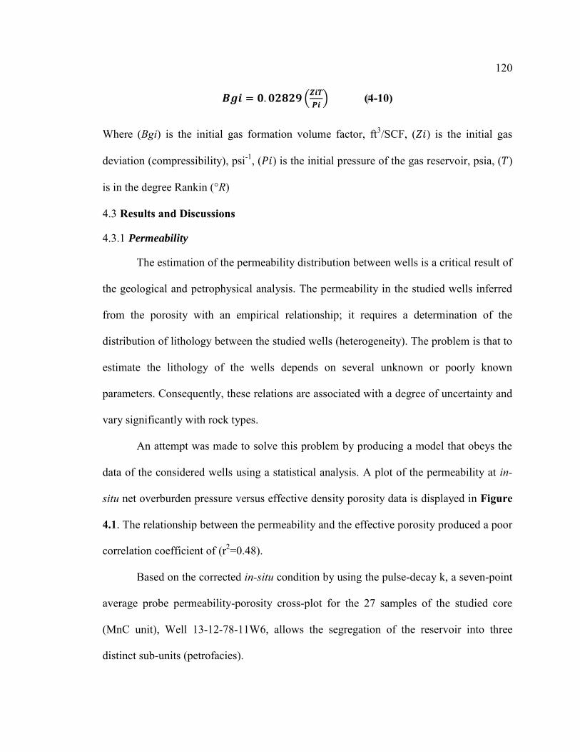
120

(

) (‎4-10)

Where (Bgi) is the initial gas formation volume factor, ft3/SCF, ( ) is the initial gas

deviation (compressibility), psi-1, ( ) is the initial pressure of the gas reservoir, psia, ( )

is in the degree Rankin (°R)

Results and Discussions 4.3

Permeability 4.3.1

The estimation of the permeability distribution between wells is a critical result of

the geological and petrophysical analysis. The permeability in the studied wells inferred

from the porosity with an empirical relationship; it requires a determination of the

distribution of lithology between the studied wells (heterogeneity). The problem is that to

estimate the lithology of the wells depends on several unknown or poorly known

parameters. Consequently, these relations are associated with a degree of uncertainty and

vary significantly with rock types.

An attempt was made to solve this problem by producing a model that obeys the

data of the considered wells using a statistical analysis. A plot of the permeability at in-

situ net overburden pressure versus effective density porosity data is displayed in Figure

4.1. The relationship between the permeability and the effective porosity produced a poor

correlation coefficient of (r2=0.48).

Based on the corrected in-situ condition by using the pulse-decay k, a seven-point

average probe permeability-porosity cross-plot for the 27 samples of the studied core

(MnC unit), Well 13-12-78-11W6, allows the segregation of the reservoir into three

distinct sub-units (petrofacies).

121

The depositional texture and the rock composition control the porosity and

permeability in conventional reservoirs. The permeability in tight gas sands, which is

characterized by fine to very fine-grained sediments, is controlled by pores and the

tortuous of pore throats connecting those pores.

In tight gas reservoirs, the relationship between the porosity and permeability is

obscured by diagenesis (alter the original pore structure), clay type and their distribution

(Rushing et al., 2008). Although, the predicted well-logs facies are most likely associated

with a particular depositional facies, the error from the overlapping ranges of the well-log

data between the facies categories that may result in misinterpretation Figure 4.2.

The predicted permeability profile from porosity was compared with the actual

laboratory measurements of the permeability for the 27 samples from the study core

(corrected profile permeability). We have two values at every sampled location, which

are a measured value and an estimated value. A reasonable trend was observed between

the measured permeability and the predicted permeability with averages of 0.0016 mD

and 0.00146 mD, respectively Figure 4.3.

To validate, a plot of the measured value versus the estimated value of the studied core

for the 27 measured samples and for the core interval are shown in Figure 4.4. For the

spread of the error up to a certain range, the sample values are overestimated; and over

that range, the sample values are underestimated.

In other words, the estimate is conditionally biased. Overall, the plots for all the sample

points over the core interval show an approximately equal number of values that are

either underestimated or overestimated. The spread of error (deviation from the straight

line) is uniform around the 45o line.

122

The magnitude of error from the measured samples and the core interval decrease

up-to-range, then the magnitude of error increases Figure 4.5. The average and median of

the estimated permeability values were 0.00146 mD and 0.00142 mD, respectively.

Whereas, the average and median of the measured permeability values were 0.00160 mD

and 0.00112 mD, respectively. As a result, the error for the average permeability was (-

0.00014 mD) which is an acceptable error range for the absolute permeability value.

123

Figure 4-1: Log-derived porosity versus permeability at reservoir net overburden

pressure (NOB) for the core measured samples (well 13-12-78-11W6).

Figure 4-2: Log-derived porosity versus permeability (7 points-averages) at

reservoir net overburden pressure (NOB) for the core interval (well 13-12-78-

11W6).

0.0001

0.001

0.01

0.02 0.03 0.04 0.05 0.06 0.07 0.08 0.09 0.1

Per

mea

bili

ty, m

D


Petrofacies 1 Petrofacies 2 Petrofacies 3

y = 0.0697x1.3359 R² = 0.48

0.0001

0.001

0.01

0.02 0.03 0.04 0.05 0.06 0.07 0.08 0.09 0.1

Pe

rme

abili

ty,

mD


Petrofacies

3

2

1

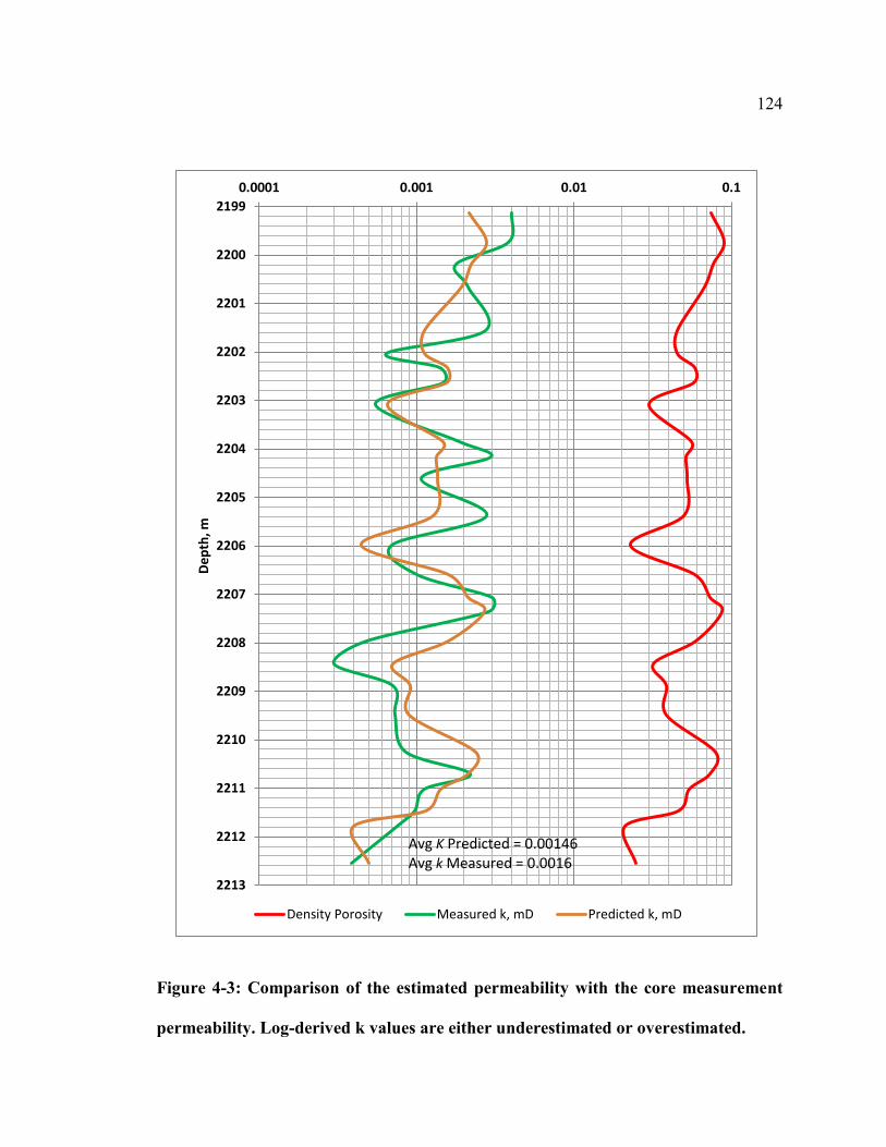
124

Figure 4-3: Comparison of the estimated permeability with the core measurement

permeability. Log-derived k values are either underestimated or overestimated.

2199

2200

2201

2202

2203

2204

2205

2206

2207

2208

2209

2210

2211

2212

2213

0.0001 0.001 0.01 0.1D

epth

, m

Density Porosity Measured k, mD Predicted k, mD

Avg K Predicted = 0.00146 Avg k Measured = 0.0016

125

Figure 4-4: Plot the measured values versus the estimated values for 27 measured

samples (A), and for the entire core interval (B).

0.0001

0.001

0.01

0.0001 0.001 0.01

Est

imat

ed k

, mD

Measured k, mD

B

0.0001

0.001

0.01

0.0001 0.001 0.01

Esti

mat

ed

k, m

D

Measured k, mD

A

126

Figure 4-5: Error versus measured value values for 27 measured samples (A), and

for the entire core interval (B).

-0.002

-0.0015

-0.001

-0.0005

0

0.0005

0.001

0.0015

0.002

0.0001 0.001 0.01

Re

sid

ual

Measured k, mD

A

-0.003

-0.002

-0.001

0

0.001

0.002

0.003

0.0001 0.001 0.01

Res

idu

al

Measured k, mD

B

127

Flow Unit Analysis 4.3.2

In order to estimate the pore throat size in the study area, the pore throat radii

lines using Aguilera’s rp35 equation were superimposed on the porosity versus

permeability. The relationship between the permeability, porosity and pore/pore throat

size is used in the recognition of the rock types and to identify the flow units Figure 4.6.

In our study area, the permeability is less than 0.1 mD; the delivery speed and the gas

diffusivity are smaller than conventional reservoirs, where k is often greater than 10 mD

(Aguilera & Harding, 2007).

Permeability increases as expected with the pore throat radius. In general, the pore

radius distribution shows that the smaller pore radius that may be indicative of very fine-

grained silts, and the composition of the sediments as well as the physical and chemical

processes. For example, calcite cementation in porous rock reduces the porosity, and

quartz and dolomite that fill the porosity, and as a result, reduces the porosity and

permeability (Freeman, 2011).

The proportion of each pore type presented depends on the organic and inorganic

composition of the rock and the pore structure that are affected by the degree of the

diagenetic alteration. The resulting pore geometry has a significant influence on the

permeability. A quantification of the pore geometry will facilitate a fundamental

understanding of the role of the reservoir heterogeneity in the MnFM in terms of fluid

flow.

The uncorrected profile permeability data fell between 0.1 and 0.2 micron rp35

lines Figure 4.6. Using the permeability correction derived from pulse-decay data

128

measured at net overburden pressure, the averages of the pore throat apertures from the

Winland rp35 plot suggest that the values lie between 0.05 µm and 0.1 µm Figure 4.7.

As a result, the scale of nano-ports size dominates in the study reservoir and

impacts production from the tight gas sand of the Montney Formation. Some of the data

lie outside of the range of 0.05 and 0.1 micron lines may reflect the lithology-dependence

of stress (Clarkson et al., 2010). The relationship between the permeability, porosity and

pore throat shows that only one hydraulic unit (flow unit) was identified Figure 4.7.

The flow unit was identified according to the dominant pore throat dimension

between (0.05 micron< r <0.10 micron) despite a wide variation in porosity. As a result,

the dominant pore throat dimensions rather than porosity control the flow speed and

capacity in reservoir rocks, helping to identify the rock quality. Decreases in pore throat

size reduce the degree of interconnectivity by increasing the tortuosity, and the

subsequent increase of disconnected pores, result in a decrease in permeability.

129

Figure 4-6: Cross-plot of the uncorrected probe permeability versus density

porosity.

Figure 4-7: Winland plot showing hydraulic rock types as a function of porosity,

permeability and the dominant pore throat size. Although, the porosity values are

varied widely, only one hydraulic rock types were observed, which lies between the

pore throat size of 0.05 and 0.1 micron for entire core interval.

0.00001

0.0001

0.001

0.01

0.1

0 2 4 6 8 10 12

Co

rre

cte

d t

o in

situ

Pro

file

Pe

rme

abili

ty,

mD

Density Porosity, %

Winland Plot

0.05 µm 0.1 µm 0.2 µmPore Size, Micron

0.00001

0.0001

0.001

0.01

0.1

1

0 2 4 6 8 10 12

Un

corr

ect

ed

Pro

file

Pe

rme

abili

ty, m

D

Density Porosity, %

Winland Plot

0.05µm 0.1µm 0.2µm 0.5µmPore Size, Micron

130

A Modified Lorenz Plot (MLP) was built for understanding the flow unit

performance and to illustrate the heterogeneity. It is simply a plot of the cumulative flow

capacity against the cumulative storage capacity in the studied core, Well 13-12-78-

11W6 Figure 4.8. This approach was useful in validating the flow units that were

determined by using the Winland plot.

The cumulative plots of (Øh) versus flow capacity (kh) for the studied core, Well

13-12-78-11W6 is a significant tool in the flow unit identification. Note that the case

which forms a 45-degree line represents a homogeneous, isotopic system. The deviation

from this line indicates heterogeneity.

By using the MLP for the data (porosity and permeability) obtained from routine

core analysis indicates the presence the heterogeneity. On the other hand, the MLP plot of

the log derived the porosity against the profile permeability for the core intervals indicate

homogeneity despite it is not in the form of a 45-degrre line.

The reason may be due to the measurements scale. Properties of the reservoir

change continuously at every scale. However, the variation in the properties at a small

level is not observed because of the averaging of the small scale properties. In other

words, the variation of a given measured property decreases as the scale of measurements

increases.

Figure 4.8 indicates that the presence of only one flow unit in the studied

reservoir (no deflection points was notified). The result confirmed in the definition of one

flow unit from the Winland plot, and also that the porosity is not the main factor to

control the permeability despite of the presence of different wide range of storage

capacity.

131

Figure 4-8: Modified Lorenz Plot shows a cumulative storage capacity versus

cumulative flow capacity from log derived porosity and profile permeability. (A) for

the routine core data, (B) for log derived porosity versus 7 point average of profile

permeability

0

10

20

30

40

50

60

70

80

90

100

0 10 20 30 40 50 60 70 80 90 100

Per

cen

t St

ora

ge C

apac

ity,

(%

Øh

)

Percent Flow Capacity, (% kh)

B

0

10

20

30

40

50

60

70

80

90

100

0 10 20 30 40 50 60 70 80 90 100

Pe

rce

nt

Sto

rage

Cap

acit

y, (

% Ø

h)

Percent Flow Capacity, (% kh)

A

MnC MnB

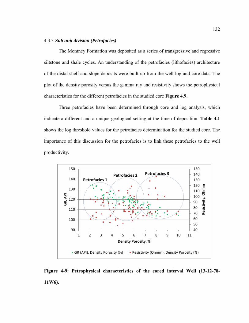
132

Sub unit division (Petrofacies) 4.3.3

The Montney Formation was deposited as a series of transgressive and regressive

siltstone and shale cycles. An understanding of the petrofacies (lithofacies) architecture

of the distal shelf and slope deposits were built up from the well log and core data. The

plot of the density porosity versus the gamma ray and resistivity shows the petrophysical

characteristics for the different petrofacies in the studied core Figure 4.9.

Three petrofacies have been determined through core and log analysis, which

indicate a different and a unique geological setting at the time of deposition. Table 4.1

shows the log threshold values for the petrofacies determination for the studied core. The

importance of this discussion for the petrofacies is to link these petrofacies to the well

productivity.

Figure 4-9: Petrophysical characteristics of the cored interval Well (13-12-78-

11W6).

40

50

60

70

80

90

100

110

120

130

140

150

90

100

110

120

130

140

150

1 2 3 4 5 6 7 8 9 10 11

Re

sist

ivit

y, O

hm

m

GR

, AP

I

Density Porosity, %

GR (API), Density Porosity (%) Resistivity (Ohmm), Density Porosity (%)

Petrofacies 3

Petrofacies 1 Petrofacies 2

133

Table ‎4-1: Hydraulic rock type by threshold value of porosity, permeability, pore

throat and lithology

Petrofacies (Lithofacies)

Description Petrophysical Properties

K mD

Ø %

Rp35 µm

GR API

Res. Ohmm

Rhob Kg/m3

Petrofacies 1 Wavy bedded with non to low bioturbated shale and mudstone

0.0004-0.002 2-4.6 0.05-0.1 >125 <80 2582

Petrofacies 2 Planar to irregular lamination of shaly siltstone

0.0005- 0.003 4.6-6.4 0.05-0.1 125 80 - 90 2579

Petrofacies 3 Coarsening and thickening up-ward siltstone to very

fine sandstone

0.0007-0.0045 6.4-10 0.05-0.1 115 >90 2566

The petrophysical measurement of the core can be used to bridge the gap between

the core and well productivity. Petrofacies (3) seems to be the best reservoir rock in the

studied units. Petrofacies (1) up-to petrofacies (3) is located in the studied core of the

Well 13-12-78-11W6 Figure 4.10.

The petrofacies (3) contains very fine sandstone-siltstone. It represents a high

quartz content and with low OM, dolomite, and calcite content from the thin section of

(TS1, TS2), which makes this reservoir relatively easy to fracture. The porosity of the

petrofacies (3) is also the highest among that of the three petrofacies. Petrofacies (3)

represents the best reservoir rock in the studied core. It has the highest porosity ranging

from 6% to 10% and permeability ranging from 0.0007 mD to 0.0045 mD.

Petrofacies (2) represents the shaly-siltstone with ripple laminations and

bioturbation. It represents the reservoir rock with a moderate dolomite and calcite

content. It also exhibits a relatively high porosity but with a low OM from the thin

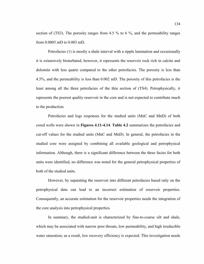
134

section of (TS3). The porosity ranges from 4.5 % to 6 %, and the permeability ranges

from 0.0005 mD to 0.003 mD.

Petrofacies (1) is mostly a shale interval with a ripple lamination and occasionally

it is extensively bioturbated, however, it represents the reservoir rock rich in calcite and

dolomite with less quartz compared to the other petrofacies. The porosity is less than

4.5%, and the permeability is less than 0.002 mD. The porosity of this petrofacies is the

least among all the three petrofacies of the thin section of (TS4). Petrophysically, it

represents the poorest quality reservoir in the core and is not expected to contribute much

to the production.

Petrofacies and logs responses for the studied units (MnC and MnD) of both

cored wells were shown in Figures 4.11-4.14. Table 4.2 summarizes the petrofacies and

cut-off values for the studied units (MnC and MnD). In general, the petrofacies in the

studied core were assigned by combining all available geological and petrophysical

information. Although, there is a significant difference between the three facies for both

units were identified, no difference was noted for the general petrophysical properties of

both of the studied units.

However, by separating the reservoir into different petrofacies based only on the

petrophysical data can lead to an incorrect estimation of reservoir properties.

Consequently, an accurate estimation for the reservoir properties needs the integration of

the core analysis into petrophysical properties.

In summary, the studied-unit is characterized by fine-to-coarse silt and shale,

which may be associated with narrow pore throats, low permeability, and high irreducible

water saturation; as a result, low recovery efficiency is expected. This investigation needs

135

a combination of capillary pressure and image analyses to verify the relationship between

the pore bodies and pore throats.

Figure 4-10: Determination of the reservoir distribution using an integrated

geological observations, core measurements and petrophysical properties. Most of

the high permeability values are associated with the core lithology of very fine-

grained sandstone and siltstones (petrofacies 3) and low values are from shale or

shaly-siltstones (Petrofacies 1), Well 13-12-78-11W6.

2199

2200

2201

2202

2203

2204

2205

2206

2207

2208

2209

2210

2211

2212

2213

40 90 140

De

pth

, m

GR, API Resistivity, Ohmm

2550 2600

Bulk Density,Kg/m^3

0.0001 0.001 0.01 0.1 1

Density Porosity

k, mD

Petrofacies 3

Petrofacies 3

Petrofacies 3

Petrofacies 3

Petrofacies 1

Petrofacies 1

Petrofacies 2

Petrofacies 2

Petrofacies 1

136

Figure 4-11: Log responses over the MnC interval, Well 13-12-78-11W6. Three

petrofacies were recognized. Petrofacies 3 represent better reservoir properties.

Petrofacies 1 has a lower reservoir quality.

217521772179218121832185218721892191219321952197219922012203220522072209221122132215

0 20 40 60 80 100 120 140 160D

ep

th, m


Density Porosity, %

2540 2590 2640 2690

Bulk Density, Kg/m3

20

200

20

200

0 1 2 3 4 5 6 7 8 9 10 11

Re

sist

ivit

y, O

hm

m

GR

, AP

I

Density Porosity, %


3 2 1

137

Figure 4-12: Log responses over the MnC interval, Well 5-14-78-11W6. Three



2500 2550 2600 2650 2700

Bulk Density, Kg/m3

20

200

20

200

3 4 5 6 7 8 9

Re

sist

ivit

y, O

hm

m

GR

, AP

I

Density Porosity, %


3 2 1

138

Figure 4-13: Log responses over the MnD interval, Well 13-12-78-11W6. Three



21282130213221342136213821402142214421462148215021522154215621582160216221642166216821702172217421762178

0 20 40 60 80 100 120 140 160

De

pth

, m

GR, API Density Porosity, %

Resistivity, Ohmm

2550 2600 2650 2700

Bulk Density, Kg/m3

20

200

20

200

0 1 2 3 4 5 6 7 8 9

Re

sist

ivit

y, O

hm

m

GR

, AP

I

Density Porosity, %


3 2 1

139

Figure 4-14: Log responses over the MnD interval, Well 5-14-78-11W6. Three



2550 2600 2650 2700 2750

Bulk Density, Kg/m3

20

200

20

200

0 2 4 6 8 10

Re

sist

ivit

y, O

hm

m

GR

, AP

I

Density Porosity, %

GR (API), Density porosity (%) Resistivity (Ohmm), Density Porosity (%)

3 2 1

140

Table ‎4-2: Log threshold petrophysical values assigned to recognize petrofacies

MnC, 13-12-78-11W6

Petrofacies GR (API) Ø (%) Res. (Ohmm) RHOB (Kg/m3) K (mD) Notes

3 100-120 4-10 70-140 2545-2595 0.0018-0.006 Relatively High

Average 110 6.6 100 2566 0.0024

2 110-130 3-8 60-130 2555-2600 0.001-0.0018 Relatively Medium

Average 118 5.4 85 2570 0.00135

1 115-130 2-7 50-85 2552-2629 0.0003-0.001 Relatively Low

Average 125 4.5 75 2592 0.0007

MnC, 5-14-78-11W6


3 84-116 6-10.3 54-112 2541-2616 0.00165-0.0034 Relatively High

Average 101 7.58 74 2584 0.00223

2 82-123 4.8-6.5 57-117 2552-2642 0.00121-0.0018 Relatively Medium

Average 107 5.76 77 2602 0.00154

1 93-120 3.1-4.9 54-190 2576-2667 0.00068-0.0013 Relatively Low

Average 108 4.4 87 2631 0.0011

MnD, 13-12-78-11W6


3 96-113 5.4-8.7 37-68 2569-22611 0.00142-0.0027 Relatively High Average 107 6.5 48 2594 0.00182

2 100-125 2.4-5.5 35-90 2588-2655 0.00047-0.0015 Relatively Medium

Average 113 3.9 55 2623 0.00092 1 103-141 <1-4 27-134 2615-2702 3.1E-07-0.001 Relatively Low

Average 117 1.5 59 2662 0.00026

MnD, 5-14-78-11W6


3 92-117 6-9.4 39-85 2567-2622 0.0016-0.003 Relatively High Average 99 7.4 48 2599 0.0022

2 91-128 3.9-6 40-90 2622-2655 0.0009-0.002 Relatively Medium

Average 103 4.8 58 2641 0.0012 1 93-127 0.04-4 40-110 2653-2713 4.4E-05-0.001 Relatively Low

Average 105 2.8 65 2637 0.0001

141

Well-log Responses and Characteristics 4.3.4

Radioactivity from the thorium and potassium content varies in the turbidite

deposits in the study area. High radioactivity is associated with the potassium feldspar

and illite. From the lithology identification plot in (Figure 3.5, chapter 3), representative

points fall between the quartz, dolomite and limestone lines.

From core, it was observed that the rock is highly heterogeneous with a lot of thin

conductive intervals. Isolated thin conductive events in the very fine sandstone and

siltstone may correspond to shale clasts and calcite cement in the surrounding pore space.

In contrast, some intervals are more resistive, reflecting the presence of hydrocarbon or

higher organic matter in homogeneous siltstone.

Laminations are of varying thickness, however, some good correlations with well

logs responses in thick intervals were observed. Although, the boundaries of the studied

units, and associated reservoir’s quality were recognized, it was not easy to detect. In

general, the bed thickness of the studied units was varying between decimeter to

centimeters.

A general upward increase in the fine-grained sandstone and siltstone content

although a general upward decrease in the bed thickness is observed, especially in the

MnC unit. In addition, the grain size and the bed thickness increase from bottom to top.

Log-correlations between the studied wells for the units of interest in the Pouce Coupe

field, WCSB is shown in Figure 4.15.

142

Figure 4-15: Electrical log correlation over Montney formation (MnC and MnD units) of Pouce Coupe area in west-central Alberta. The composite-log responses do not easily detect the boundary between

facies. In cores interval, Wells 13-12-78-11W6 and 5-14-78-11W6, the responses show increases in very fine sandstone and siltstone content by decrease in GR signatures.

2115

2120

2125

2130

2135

2140

2145

2150

2155

2160

2165

2170

2175

2180

2185

2190

2195

2200

2205

2210

2215

30 300D

ep

th, m

5-14-78-11W6

GR ILD

2125

2130

2135

2140

2145

2150

2155

2160

2165

2170

2175

2180

2185

2190

2195

2200

2205

2210

2215

2220

30 300

13-12-78-11W6

GR RT

2100

2105

2110

2115

2120

2125

2130

2135

2140

2145

2150

2155

2160

2165

2170

2175

2180

2185

2190

2195

30 300

16-12-78-11w6

GR SFLU

2140

2145

2150

2155

2160

2165

2170

2175

2180

2185

2190

2195

2200

2205

2210

2215

2220

2225

2230

30 300

3-12-78-11W6

GR ILD

2130

2135

2140

2145

2150

2155

2160

2165

2170

2175

2180

2185

2190

2195

2200

2205

2210

2215

2220

30 300

2-2-78-11W6

ILD GR

2215.8 m1147.1 m1187.5 m1679.6 m

M

n

D

M

n

C

143

Estimating Net Pay and Estimated Initial Gas-in-Place 4.3.5

The net pay estimation is one of the most important steps in evaluating the

resources. The net pay can be influenced by: i) quality and amount of log, core, test data;

ii) the nature of rock and fluids system; iii) recovery mechanism (Cronquist, 2001). The

gross interval for the studied units was determined by establishing the top and bottom of

the zones of interest.

In the studied units, the midpoint of the GR, resistivity and porosity deflections

were considered to be boundaries of units. The non-pay intervals within the gross interval

were excluded by using a minimum porosity and permeability cutoff, maximum water

saturation and shale cutoff.

To identify the net pay, the porosity and permeability relationship for the unit

MnC was established through the calibration of logs to the 13-12-78-11W6 core to

determine the porosity cut-off values. The k-Ø correlation leads to the concept of the

critical or cutoff porosity.

Based on the values for the average permeability (kc) and average porosity (Øc) of

the three different petrofacies, the cross-plot of porosity versus permeability was divided

into four regions. Region (A) represents non-pay (k<kc & Ø<Øc). In contrast, region (D)

represents net pay region (k>kc & Ø>Øc). Regions (B) and (C) are misidentifications for

non-pay when using Ø to compare with Øc, where (k>kc & Ø<Øc) or (k<kc & Ø>Øc)

Figure 4.16.

Unfortunately, this method may not always be the best estimate method. The best

estimate of Net-To-Gross-Ratio (NTG) requires selecting Øc with equal probabilities of

(C) and (B), regardless of their magnitudes. The NTG represents correct NTG value due

144

to the errors cancel out in the regions (B) and (C). The error probability is the ratio of the

number of the sample point in (C) or (B) divided by the total sample point. The best

estimates for Øc to minimize the errors are based either to minimize the sum of the

probabilities (C) and (B) or maximize the sum of the probabilities of (A) and (D).

However, the kc line has been shifted instead to minimize the errors and to get the

best estimation of the permeability cut-off value, which is called (kBE). The best estimate

for Øc is obtained by related Øc into (kBE) rather than related of Øc into kc, which are

0.00125 mD and 0.0016 mD, respectively. The standard deviation from the average of

the predicted permeability kc is within a range of (± 0.00066 mD).

Figure 4-16: Cutoff value estimation using the relationship between permeability

and porosity for the core samples. The dotted lines indicate the standard error band

of (± 0.00066 mD).

0.0001

0.001

0.01

0 0.02 0.04 0.06 0.08 0.1

Pe

rme

abili

ty,

mD

Porosity, Fraction

D B

C

Øc Kc KBE

A

145

By combining all the geological core, petrophysical and statistical available

information leads to the conclusion that the relationship between kBE and Øc are

reasonable cut-off values. In addition, the relation between kBE and Øc gives an optimistic

estimate for NTG compared to the relationship between Øc and kc.

The errors for the sample points are reduced by maximizing the correct

probability or minimizing the error probability. Table 4.3 summarizes the different

values of Øc, kc, and kBE with their error rate (probability of making an error for

regions(C) and (B)). These statistical analysis shows that the different cutoffs are

different in statistical sense.

Table ‎4-3: Demonstrates the different estimation for kc and Øc for the studied wells

The net pay estimation is easy to discuss but it is difficult to quantify; however,

the procedures for computing the net pay are very limited or do not exist for low

permeability reservoirs. The determination of the NTG ratio is one of the typical steps in

any reservoir study, which is practically always performed. Therefore, the integrated data

(geological, geophysical and reservoir engineering) will produce an interpretation of data

and the properties of each reservoir Figure 4.17.

Kc Non Pay (Ø<0.054), 14 points (Probability=0.518)

Pay (Ø>=0.054), 13 points (Probability=0.481)

0.00160 K<0.00160, 11 points K>=0.00160, 3 points K<0.00160, 5 points K>=0.00160, 8 points

Correct =0.407 Error =0.111 Error =0.185 Correct =0.296

KBE Non Pay (Ø<0.054), 14 points (Probability=0.518)

Pay (Ø>=0.054), 13 points (Probability=0.481)

0.00125 K<0.00125, 11 points K>=0.00125, 3 points K<0.00125, 3 points K>=0.00125, 10 points Correct =0.407 Error =0.111 Error =0.111 Correct =0.370

146

The relationship between k and the petrophysical data is used to evaluate the

NTG. Table 4.4 summarizes the different results of the NTG ratio from the geological

observation to that of the estimated NTG based on the integrated geological observation

to the petrophysical analysis, which was applied in the studied case.

Table ‎4-4: Summarizes the different results for estimating the NTG by different

methods- geological observation versus integrating geological and petrophysical

data. (CGT) Core gross thickness, (NST) Net fine-grained sandstone and siltstone

thickness, (NsTCG) Net sandstone and siltstone to core gross thickness, (NPT) Net

pay thickness, (NTG) Net pay to gross ratio

Well ID NTG (Kc = 0.00125 mD, Øc = 5.4 %)

13-12-78-11W6

Physical measurement over cores

intervals

Integrated data over the cores

intervals

CGT NST NsTCG NST NsTCG NPT NTG

13.41 4.10 0.305 7.23 0.54 5.18 0.39

147

Figure 4-17: Comparison of the computed log permeability and measured

permeability, Well 13-12-78-11W6. The Net-to-Gross ratio has been estimated by

using porosity and permeability parameters.

2199

2200

2201

2202

2203

2204

2205

2206

2207

2208

2209

2210

2211

2212

2213

0.0001 0.001 0.01 0.1 1D

ep

th, m

Density Porosity Measured k, mD Predicted k, mD

Øc = 0.054 KBE = 0.00125 mD

CGT = 13.41 m

NPT = 5.18 m

NTG = 0.39

148

An attempt has been made to estimates the gas-in-place for the studied wells. The

input petrophysical parameters for the estimation of the resource were provided from the

calculations in the current study. Each of the studied units was evaluated separately by

calculating the average of the parameters in the selected wells. Table 4.5 summarized

input of engineering parameters that provided in Clarkson & Beierle (2010).

Table ‎4-5: Input engineering parameter from Clarkson and Beierle (2010)

Parameters

Total Compressibility (zi), psi-1 1.89×10-4 Reservoir Temperature (T), F° 200

Initial Reservoir Pressure (pi), psia 3300

The Bgi (initial gas formation volume factor) was calculated using engineering

input as long with the calculated area of the studied wells (640 Acres) using geo-scout

tools. Bgi is equal to 1.07×10-6 ft3/SCF. Initial gas in place was then calculated based on

the average of the petrophysical parameters (porosity, water saturation, net pay thickness)

that were calculated in the current study.

As a result, the initial gas in place ( ) using the volumetric method for both

units in the studied wells was estimated to be in summation of 8.05×1011 scf per section

(one acre unit). However, the estimated initial gas in place for the unit MnC is bigger

than that was estimated for the MnD, which are 5.92×1011 scf and 2.13×1011 scf,

respectively. The result was expected due to a higher porosity and net pay thickness, and

lower water saturation in the unit MnC than the unit MnD.

149

Table 4.6 shows the petrophysical parameters used for the gas-in-place

calculation for both units. Gas-in-place is estimated for each well and is calculated per

one acre unit. The gas-in-place is estimated based on the petrophysical properties, Well

16-12-78-11W6, however, has the highest ( ) among the studied wells from both

units.

Well 13-12-78-11W6, in contrast, has the lowest ( ) among the studied wells

from both of the studied units. The gas-in-place estimation from the MnC unit in the Well

13-12-11W6 is the lowest, while; the gas-in-place estimation from the MnD unit in the

Well 5-14-11W6 is the lowest.

Table ‎4-6: Petrophysical parameters for estimated initial gas-in-place

Well MnC MnD OGIP

(scf)

OGIP

(scf) Ø

Frct.

h

ft

Swg

Frct.

Ø

Frct.

h

ft

Swg

Frct.

13-12-78-11W6 0.046 60.50 0.77 0.028 50.49 0.53 8.73×1010

3.05×1010

5-14-78-11W6 0.055 59.15 0.82 0.017 53.15 0.39 1.08×1011

1.44×1010

3-12-78-11W6 0.053 66.44 0.88 0.031 56.59 0.71 1.27×1011

5.21×1010

16-12-78-11W6 0.061 74.64 0.89 0.035 70.13 0.67 1.67×1011

6.70×1010

2-2-78-11W6 0.051 55.36 0.88 0.027 62.33 0.70 1.01×1011

2.11×1011

Average 0.053 63.22 0.85 0.028 58.54 0.60 Sum Sum

5.92×1011

2.13×1011

150

Relationship between horizontal permeability (KH) and vertical permeability (KV) 4.3.6

Horizontal (KH) and vertical (KV) permeability are determined from core, and the

petrophysical (porosity-permeability) analysis on a regular basis. (KH) and (KV) can be

determined accurately from special test conditions. The average porosity was plotted with

log analysis-derived horizontal permeability and vertical permeability for each of the

studied wells in Figure 4.18.

In general, the average porosity and permeability for the unit MnC are higher than

of the unit MnD; and KV for the studied wells was less than KH in both units for the

studied wells. In addition, the result of the permeability from the core measurements and

the permeability from the log-derived data for the core interval, Well 13-12-78-11W6 is

comparable. The average KH from core measurements and log-derived-permeability are

0.154 mD and 0.00147 mD, respectively. On the other hand, KV from core measurements

and log-derived-permeability are 0.111 mD and 0.00115 mD, respectively.

Figure 4.19 shows an acceptable correlation of KV and KH values obtained from

well logs measurements. The correlation relating KV to KH depicts the degree of

anisotropy, especially in the MnD. Anisotropy means that the permeability is direction

dependent.

Consequently, the average permeability is less than the max permeability in any

direction in the reservoir. However, the petrophysical properties variation varies from the

pore level to megascopic heterogeneity. Therefore, the petrophysical properties are better

understood by using the scale of heterogeneity.

151

Figure 4-18: Relationship of porosity with vertical and horizontal permeability.

Figure 4-19: Vertical-horizontal permeability relationship in the studied wells.

y = 88372x2.9142 R² = 0.7731

0.000003

0.00003

0.0003

0.003

0.0002 0.002

Kv,

mD

Kh, mD

MnC MnD

0.000001

0.00001

0.0001

0.001

0.01

1.5 2.5 3.5 4.5 5.5 6.5

K, m

D

Porosity, %

Vertical Permeability, mD Horizontal Permeability, mD

5-14-78-11W6 13-12-78-11W6 3-12-78-11W6

16-12-78-11W6

MnD MnC

152

Comparison of estimated k from petrophysical analysis and production data 4.3.7

Correlation of the petrophysical data with the in-situ rock property data allows for

quantitative assessments of the reservoir properties such as hydrocarbon-in-place and

reservoir deliverability. The petrophysical data can be used in order to tie the geological

description with the production data and can reduce the need for additional core data and

well-test data.

The challenge is that conventional well-tests for tight gas sands face practical and

economic problems. A long time is required to reach the infinite-acting radial flow

because of the low permeabilities associated with these reservoirs such as in the Montney

Formation.

Production data analysis has been applied for the extraction of the permeability-

thickness product (kh) and hydrocarbon in place (Poe et al., 1999). Production data and

rate-transient analysis methods, including the flow-regime and type-curve methods have

been applied for the existing well data in order to establish reservoir and hydraulic

fracture properties (Clarkson and Beierle, 2011).

Log-derived estimates of kh are compared with kh from the production data, the

latter being obtained from Clarkson and Beierle (2011). Table 4.7 shows estimates of kh

for Wells 16-12-78-11W6 and 3-12-78-11W6 using the petrophysical analysis, and

production data. For production data analysis, estimates from the Type-Curve (T-C) and

Straight-Line (S-L) were obtained (Clarkson and Beierle, 2011).

The commingled production data were analyzed by Clarkson and Beierle (2011),

so the kh estimate represents a performance-based composite value of the two zones

(MnC and MnD). KH and NTG for both units in Well 16-12-78-11W6 are higher than KH

153

and NTG for Well 3-12-78-11W6. However, the expectation is that kh will be higher for

Well 16-12-78-11W6 than 3-12-78-11W6.

Table ‎4-7: Comparison for k estimation by using petrophysical analysis to k

estimation by production data

Wells Production Data Analysis (md.ft)

Petrophysical Analysis (md.ft)

kh T-C

k T-C

kh S-L

k S-L

kh k

3-12-78-11W6 1.0 0.011 0.85 0.009 0.20 0.0052 16-12-78-11W6 0.62 0.012 1.3 0.024 0.275 0.0065

The results show that the estimated k from the production data is higher than

estimated k from the petrophysical analysis in the studied wells. Also, the estimated k by

type-curve analysis was higher than estimated k by straight-line analysis. In terms of the

production data the reasons were due to:

i) The permeability value from the production data was estimated

using the assumption for the net-pay provided by kh from the radial flow. The

assumption of the gross thickness was assumed to be confined to the estimated

propped fracture height obtained from the tracer logs. The net pay is then

evaluated based on the porosity cut-off value. However, the net pay from the

production data may be underestimated. Consequently, the estimated

permeability in the investigated wells could be overestimated (Clarkson &

Beierle, 2010).

154

ii) Net pay underestimation may also be due to the productive zones

being blocked by water due to the capillary pressure forces, which affects the

relative permeability.

iii) Due to the extremely low permeability, the radial flow was

definitely not reached during the analysis of the studied wells. The estimated

permeability may be biased to layers that are characterized by high

permeability in the early stages of the well or the production test (Clarkson &

Beierle, 2010). As a result, this can have an impact on the reserve estimation

(overestimation) for tight gas sands due to uncertainty of the drainage area.

iv) Improper completion due to non-isolation pay zones; poor cement

quality or the bond between the production casing and reservoir rocks is not

effective. Therefore, the production can be from other permeable zones out of

the interested zones.

v) The possibility of the presence of natural fractures within the

reservoir which are undetected by using standard well logging tools. The

presence of the natural fractures influences the production by increasing the

gas flow of gas to the borehole.

In terms of the petrophysical analysis, the variation of estimated k by the

production data to the petrophysical analysis because of:

i) Net-pay thickness was evaluated by petrophysical properties, and

porosity- permeability cut-off values. In other words, although the net pay has

been estimated, the MnFM can be produced from any portion due to the

reservoir heterogeneity.

155

ii) Only matrix porosity was considered in this study (no fracture was

observed in the cores and thin sections). Although, there is not real evidence

of natural fractures from the core or production data, there may be some

contribution to the flow from the fractures that go undetected.

iii) Maybe some gas was desorbed in the organic matter. However, to

estimate the produced portion from shale to silty-shale interval was a difficult

task using only wire-line logs.

iv) The production data was measured for the MnC and MnD together.

The petrophysical parameters are mainly correlated to the MnC because of

sampling of this zone with the cores. However, the parameters estimated from

the MnC were used for evaluating the MnD. Consequently, there is a resulting

uncertainty in evaluating the petrophysical properties due to the differences in

the matrix, shale volume, water resistivity, shale resistivity between the MnC

and MnD.

The cut-off values for the porosity and permeability for the net pay estimation of

each unit for the studied wells are shown in Figures 4.20-4.27. The figures, in general

show that the porosity and permeability increases when the GR log decreases. This may

indicate the porosity and the GR logs combination are related to the permeability. In

addition, the unit MnC show better reservoir quality compared to the unit MnD. Tables

4.8 and 4.9 summarize the petrophysical properties porosity, Ke, and the Net-to-Gross

ratio for both the studied units in each well.

156

(MnC for Well 13-12-78-11W6)

Figure 4-20: Permeability is related to porosity, as the porosity increases, the

permeability increases. High GR accompanies low permeability. This may suggest

narrow pore radius due to pore lining/bridging clay.

2178

2180

2182

2184

2186

2188

2190

2192

2194

2196

2198

2200

2202

2204

2206

2208

2210

2212

2214

0.00010.001 0.01 0.1 1 10 100

De

pth

, m

K, mD Porosity, %

Øc=4.6 %

Kc=0.0012 mD

157

(MnD for Well 13-12-78-11W6)

(MnC for Well 5-14-78-11W6)




2128

2130

2132

2134

2136

2138

2140

2142

2144

2146

2148

2150

2152

2154

2156

2158

2160

2162

2164

2166

2168

2170

2172

2174

2176

2178

0.0000001 0.00001 0.001 0.1 10D

ep

th, m

K, mD Porosity, %

Øc=2.8 %

Kc=0.00067 mD

158





2174

2176

2178

2180

2182

2184

2186

2188

2190

2192

2194

2196

2198

2200

2202

2204

2206

2208

2210

0.00010.001 0.01 0.1 1 10 100D

epth

, m

Porosity, % K, mD

80 90 100 110 120 130

GR, API

Øc=5.5 %

Kc=0.0015 mD

159

(MnD for Well 5-14-78-11W6)





2118

2120

2122

2124

2126

2128

2130

2132

2134

2136

2138

2140

2142

2144

2146

2148

2150

2152

2154

2156

2158

2160

2162

2164

2166

2168

2170

2172

2174

1E-090.00000010.00001 0.001 0.1 10D

ep

th, m

Porosity, % K, mD

90 100 110 120 130

GR, API

Øc=1.7 %

Kc=0.00035 mD

160

(MnC for Well 16-12-78-11W6)




2104

2106

2108

2110

2112

2114

2116

2118

2120

2122

2124

2126

2128

2130

2132

2134

2136

2138

2140

2142

2144

2146

2148

2150

0.00000010.00001 0.001 0.1 10D

ep

th, m

Porosity, % K, mD

90 100 110 120 130

GR, API

Øc=6.2 %

Kc=0.0017 mD

161

(MnD for Well 16-12-78-11W6)




2148

2150

2152

2154

2156

2158

2160

2162

2164

2166

2168

2170

2172

2174

2176

2178

2180

2182

2184

2186

2188

2190

1E-050.0001 0.001 0.01 0.1 1 10D

ep

th, m

Porosity, % K, mD

90 100 110 120 130 140 150

GR, API

Øc=3.5 %

Kc=0.00087 mD

162





2185

2187

2189

2191

2193

2195

2197

2199

2201

2203

2205

2207

2209

2211

2213

2215

2217

2219

2221

2223

0.0001 0.001 0.01 0.1 1 10D

ep

th, m

Porosity, % K, mD

80 90 100 110 120 130

GR, API

Øc=5.37 %

Kc=0.0014 mD

163




permeability increases. High GR accompanies with low permeability. This may

suggest narrow pore radius due to pore lining/bridging clay.

2140

2142

2144

2146

2148

2150

2152

2154

2156

2158

2160

2162

2164

2166

2168

2170

2172

2174

2176

2178

2180

2182

2184

0.000010.00010.001 0.01 0.1 1 10

De

pth

, m

Porosity, % K, mD

80 90 100 110 120

GR, API

Øc=3.18 %

Kc=0.00073 mD

164

Table ‎4-8: Summary of permeability prediction and pay thickness estimation from

petrophysical analysis for unit MnC

13-12-78-11W6

Avg. KH, mD Avg. KV, mD Kc, mD (Kh)wt, mD-m Kh, mD-m Ke, mD 0.00122 0.00019 0.00122 0.0478 0.0342 0.00185

Øc, % Gross Intv., m Net Pay, m NTG 4.6 39.17 18.44 0.47

5-14-78-11W6



3-12-78-11W6



16-12-78-11W6



2-2-78-11W6



165

Table ‎4-9: Summary of permeability prediction and pay thickness estimation from

petrophysical analysis for unit MnD

13-12-78-11W6

Avg. KH, mD Avg. KV, mD Kc, mD (Kh)wt, mD-m Kh, mD-m Ke, mD 0.00067 2.58e-05 0.00067 0.0296 0.021 0.00135


5-14-78-11W6



3-12-78-11W6



16-12-78-11W6



2-2-78-11W6


Øc, % Gross Intv., m Net Pay, m NTG 2.78 51.13 19 0.37

166

Although petrophysically, Well 2-2-78-11W6 is comparable to the other four

studied wells, the well is not producing from the MnFM. Well 2-2-78-11W6 is producing

from the Triassic Doig Formation. An attempt has been made to investigate the reasons if

why Well 2-2-78-11W6 is not producing from the MnFM.

In addition, two wells were chosen in the between producing Well 3-12-78-11W6

and well 2-2-78-11W6. The chosen Wells were 100/1-1-78-11W6 and 102/3-1-78-11W6.

The measured distance between Wells 100/1-1-78-11W6 and 102/3-1-78-11W6 to Well

2-2-78-11W6 are 2176.02 m and 1376.45 m, respectively. The distance between 100/1-1-

78-11W6 and 102/3-1-78-11W6 and 3-12-78-11W6 is 1923.93 m and 1734 m,

respectively.

Table 4.10 summarized the production information for the studied wells. 3-12-78-

11W6 and 16-12-78-11W6 have produced of 14,800 up-to 24,000 e3m3 gas in period of 5

years (2006-2011) from the Montney. On the other hand, Well 2-2-78-11W6, which is

within a 4 km distance from the previous mentions wells, have produced 187,261 e3m3 of

gas in a period of 17 years from the Triassic Doig Formation.

The other two Wells, 1-1-78-11W6 and 3-1-78-11W6, were chosen to be in

between the above three wells. Well 1-1-78-11W6 is producing from the Lower Montney

Formation, from the Lower Cretaceous Gething Formation and from the Middle Triassic

Doig Formation produced 10,525 e3m3 of gas for period of 5 years. Well 3-1-78-11W6 is

producing only from the Lower Montney Formation, with 10,611 e3m3 of gas for period

of 5 years.

167

Table ‎4-10: Summary of production data for the studied wells

Well ID Cum. Production First 12 months total cum. Production

Last 12 months total cum. Production

G (e

3m

3)

C (m

3)

W (m

3)

Gas (e

3m

3)

Gas (e

3m

3)

2-2-78-11W6 187,261.0 486.0 1307 32,220.0 2709.0 Note Spud, 24.1.1994, Cmpl., 9.2.1994 - Hist. Prod. (1994-2011)-Perforated and Fractured in

TRdoig at depth (1922.7-1941.7m) 3-12-78-11W6 14,798.4 335.9 216.3 6410.0 2452.2

Note Spud, 15.1.2006, Cmpl., 24.1.2006 - Hist. Prod. (2006-2011)-Perforated and Fractured in MnFM at depths (2216-2220m (MnC), and 2153.5-2156.5m (MnD))

16-12-78-11W6 24,138.0 739.0 933 6454.0 579.5 Note Spud, 7.3.2003, Cmpl., 22.3.2003 - Hist. Prod. (2006-2011)-Perforated and Fractured in

MnFM at depths (2205.2-2023.8m, 2200-2202m, and 2123-2125m (MnD)) 1-1-78-11W6 10,525.0 358.2 306 4935.0 1767.0

Note Spud, 15.1.2006, Cmpl., 24.1.2006 - Hist. Prod. (2006-2009)-Perforated and Fractured in MnFM at depths (2247-2250m, 2181-2184m, and 2075-2078m)

3-1-78-11W6 10,611.0 205.3 193.9 3725.0 1499.5 Note Spud, 29.11.2005, Cmpl., 10.12.2005 - Hist. Prod. (2006-2011)-Perforated and

Fractured in MnFM at depths (2238.5-2241.5m, and 2166-2169m)

The following is an evaluation of the 2-2-7811W6 well, which did not produce

from the Montney Formation, and the factors that could impact the production from the

well in the Montney:

i) The Well 2-2-78-11W6 has comparable lithology from (well log responses),

and petrophysical properties (porosity, water saturation, grain density) and the

permeability to the producing Wells 16-12-7811W6 and 3-12-7811W6. As a

result, the well is expected to be able to produce as much as the reference

production wells.

ii) The production from the gas shale and tight sand are still in the initial stages

of evaluation. In addition, the non-conventional methods are essential for

reservoir analysis, drilling, completion, stimulation and production from such

168

reservoirs. There is a high uncertainty in the resource estimates even at the

current time.

iii) The Well 2-2-78-11W6 was produced more from the Doig Formation in the

last year (2700 e3m3) compared to the best well in the group of four wells, 3-

12-78-11W6 by (2450 e3m3). In addition, based on the information from

Geoscout, the well was vertically drilled and spudded in 1994. However,

drilling in the Montney Formation requires advanced methods (horizontal

drilling and hydraulic fracturing) to analysis the reservoir properties and

increase the production from wells and that will be at a far higher cost

(approximately 5 to 8 million dollars per well) due to additional time required

for drilling (NEB, 2009).

iv) Finally, the environmental concern associated with the development of

shale/tight gas sands. Little is known about the impact on the freshwater

resources by using chemicals additive that carry an injected proppant. Fluid

such as water, propane, and CO2 or nitrogen gas are pumped down the well

loaded with the proppant to create cracks in the reservoir. Therefore,

recovered frac water when the wells produce gas must be treated or disposed

safely (NEB, 2009).

Conclusion 4.4

The MnFM in the study area presents the evaluation challenges due to

heterogeneity (alternating laminations) and the impact of the diagenesis. However,

understanding the log measurement allows us to evaluate the multiple scenarios and

169

provides a more comprehensive understanding of the reservoir characterization, which

includes the lithological and fluid property characterization.

There is a significant potential for the unconventional tight sand/shale gas

production from the MnFM. However, there is much uncertainty because the shale gas is

currently under the early stages of the discussion and investigation. Maximizing gas the

recoveries requires non-traditional methods of exploitation, including the use of multi-

fractured horizontal wells.

In order to understand the reservoir quality and to correlate between the wells,

non-routine methods were applied, including the non-routine lab data and techniques to

determine the relationship between the reservoir parameters and permeability for all

wells. Integrating the porosity, permeability, for the units, rock types and the geologic

framework is a better than the traditional net pay method.

A specific relationship between the porosity and permeability was established.

The estimated porosity in the studied wells was a reasonable predictor of permeability.

The predicted permeability was matched to the corrected profile permeability

measurements from the core samples (slight difference between the averages of k values).

The accuracy of the permeability prediction is limited by the accuracy of the

geologic and petrophysical models. In other words, although, the porosity was reasonably

correlated with k, the porosity alone is not an accurate delimiter for recognizing the net

pay in the studied units.

Measurement of the dominant pore throat dimension improved and enhanced the

permeability prediction. The application is extended over the non-cored wells. Horizontal

permeability is higher than the vertical permeability for both units in the studied wells. In

170

addition, the unit MnC has a better reservoir quality compared to the unit MnD due to

higher porosity, permeability, low GR log and consequently thicker pay interval. The

horizontal permeability and net pay thickness is used for estimation of kh.

Unfortunately, due to the heterogeneities and low resolution of the conventional

wire-line logging tools, up-scaling of laminations in the studied wells was a difficult task.

Moreover, estimating permeability by using conventional well-test continues to be a

challenge for unconventional gas reservoirs because the radial flow period is rarely

reached.

As a result, an attempt was made to combine and investigate the available static

and dynamic properties for the studied reservoir. The methods and approaches presented

in this work for the finely-laminated siltstone and shale of the Montney tight gas reservoir

produced a quantitative estimate of permeability and did create suitable scales for the

reservoir despite the variation in the permeability measurement by the core measurements

and petrophysical analysis to the engineering evaluation.

171

Conclusions and Recommendations Chapter Five:

Over the last several years, unconventional gas reservoir development has rapidly

increased. In this thesis, a quantitative methodology for the reservoir characterization that

improves the prediction of permeability, flow unit definition, and rock typing through the

integration of quantitative geological and petrophysical data was provided.

This study uses an integrated approach to the petrophysical research and to

evaluate the tight gas reservoirs, specifically, the Lower Triassic Montney Formation,

West-Central Alberta (Pouce Coupe Field) from the Western Canada Sedimentary Basin

is used an example. The Lower Montney Formation is dominant with siltstone. The

Montney Formation has been divided into three members, the lower sandstone, middle

coquina dolomite and upper siltstone and shale associated with turbidite deposits.

Conventional methods for reservoir property evaluation are not applicable to the

unconventional reservoirs. This study was conducted to review and apply the laboratory

analyses and the wire-line log data of the MnFM reservoir. The study was done based on

the core measurements, and petrophysical responses from the wire-line logging tools.

The conventional well logs and core calibration is useful to identify the facies

variation. 13-12-78-11W6 core divided into two in-formal facies (units), which are the

MnC and the MnB. The units were interpreted to be a fan-fringe and basin plain turbidite

deposits (Freeman, 2011).

Due to of the existence of the variation in permeability, profile (probe)

permeability was conducted to characterize the heterogeneity of the reservoir (Clarkson

et al., 2010). The profile permeability is higher than the reservoir-condition permeability

because it was measured at nearly zero stress. The profile permeability was therefore,

172

corrected to the in-situ condition by using the pulse decay permeability measurements

that were performed on the core plugs cut at the location of the profile measurements.

The results revealed a statistically reasonable correlation between the wire-line log

analysis and the measured permeability.

The wire-line log analysis, once calibrated with the core measurements, is a very

useful tool in extending the reservoir understanding. Understanding log measurements

and interpretation uncertainties allows for the evaluation of the reservoir properties. An

integrated petrophysical approach has been developed by using multiple logging

technologies to characterize the reservoir lithology and mineralogy, porosity, water

saturation, permeability and to calculate the original gas-in-place volume.

Pore geometrical measurements allow for improvements in the prediction of the

permeability distribution from the wire-line logs within the cored intervals, non-cored

intervals and adjacent wells. In addition, it allowed for the definition of the hydraulic

units which can be related to the logs for useful field studies. Further, it can be used for

the prediction of reservoir quality and rock type for proper completion.

In summary, the reservoir characterization efforts and results are integrated in the

geological, petrophysical and production test data will be directed for the accurate

assessment of the reservoir properties and their distributions, and to explore the

feasibility of developing these resources with new technology such as horizontal wells

and hydraulic fractures create a high conductivity pathway to the well for the gas to flow

through.

173

From this study, the following conclusions are drawn for the Montney Formation

at the Pouce Coupe in particular, based on the combination of the logging measurements

and the cores analyses:

1. The study has mainly been applied with a comprehensive data on one core.

However, more wells which include cores and well logs data and

measurements such as the shale and water resistivity, and the saturation

exponent cementation factor for the MnC and the MnD units would need to be

done to verify the distribution of the reservoir properties.

2. Routine core analysis consists of the permeability measurements taken at

relatively low pressure, which is not representative of the in-situ condition.

Permeability decreases significantly with confining (overburden) stress by an

average of 60%.

3. Gas occurs in the low-permeability, poor-quality reservoir characterized by

the unique petrophysical properties due to the thinly interbedded siltstone and

shale from one to several centimeters in thickness and of variable quality.

4. Traditional interpretation techniques fail when conducted on the

unconventional MnFM reservoir due to variations in the matrix mineralogy,

partial fluid invasion, diagenesis and compaction, and formation clay.

5. Pore-throat sizes are used to define the flow units. Only one flow unit was

recognized in the Well 13-12-78-11W6 by using Winland and the MLP plots.

The pore-throat diameter in the studied unit range from 0.05 to 0.1 µm.

6. Three petrofacies are observed from the petrophysical measurements.

Petrofacies 3 represents the best reservoir rocks and petrophysical properties.

174

Petrofacies 2 is a moderate reservoir rock, while petrofacies 1 represents the

lowest quality reservoir with the expectation of the lesser contribution for the

gas production.

7. To estimate the part of a succession that contributes significantly to the

hydrocarbons in place or the ultimate hydrocarbon recovery, cut-off values for

the reservoir parameters are needed. The net pay and gas in place was

estimated from the logs responses of the static properties and an attempt has

been made to relate the static to dynamic reservoir properties.

The following recommendations for further work are suggested:

1. Understanding the relationship between the pore geometry and the routine

versus special core measurements under the overburden condition are required

to characterize the low-permeability reservoir behaviour.

2. Unconventional reservoirs require to collect and to integrate geological,

petrophysical and engineering data. Integration of the available information

can enhance the correlation between the measured parameters and various

techniques.

3. Due to heterogeneity, spatial variations and thin laminations, the non-

traditional analysis methods such as the non-routine core measurements, and

new technology development such as logging tools characterized by a high

resolution are required. For example FMI (Formation Micro Imager) to refine

a routine lithological interpretation by defining the thin beds at a finer scale;

measurement of the sedimentary structure orientation; provide a detailed

textural information and bed boundaries. Quantitatively, can be used to

175

quantify the bed thickness of the thin beds; quantify the porosity and

permeability by producing the image of permeability distribution across the

core slabs if the sufficient mini-permeameter readings are taken (Rider, 2000).

DSI (Dipole Sonic Imager) could make a significant contribution to reservoir

understanding. It allows for us to identify and measure of fractures type in the

subsurface. It can detect down to a width of 0.025 mm (0.001 inch). However,

using the acoustic imaging with the flow-meter readings can be used for

located the fractures and to separate the flowing fracture from the non-flowing

ones (Rider, 2000).

4. Statistical-optimization, response equation based approaches are very

powerful, but they are often very difficult to use in such reservoirs. Neural

networks (ANN) may provide better prediction accuracy than response-

equation-based interpretation approaches. ANN can learn non-linear

relationship, even if the input data is noisy and less precise such as

geophysical well-log data. Some of application in the petroleum industry

include permeability prediction, lithofacies identification and gas well

production analysis and improvement (Ali, 1994).

176

BIBLIOGRAPHY

Aguilera, R. (2002). Incorporating Capillary Pressure, Pore Aperture Radii, Height

Above Water Table, and Windland r35 Values on Pickett Plots. AAPG, 605-624.

Aguilera, R. (2010). Flow Units: From Conventional to Tight Gas to Shale Gas

Reservoir. Trinidad and Tobago Energy Resources Conference . Port of Spain,

Trinidad: SPE 132845.

Aguilera, R., & Harding., T. (2007). State-of-the-Art of Tight Gas Sands Characterization

and Production Technology. Petroleum Society's 8th Canadian International

Petroleum Conference (58th Annual Technical Meeting). Calgary, Canada:

Petroleum Society Journal.

Ahmed, U., Crary, S., & Coates, G. (1991). Permeability Estimation: The Various

Soyrces and Their Interrelationships. JPT, 578-586.

Ali, J. (1994). Neural Networks: A New Tool for the Petroleum Industry. European

Petroleum Computer Conference (pp. 217-231). Aberdeen, U.K.: SPE 27561.

Amaefule, J., Altunbay, M., Tiab, D., Kersey, D., & Keelan, D. (1993). Enhanced

Reservoir Description: Using Core and Log Data to Identify Hydraulic (Flow)

Units and Predict Permeability in Uncored Intervals/Well. Annual Technical

Conference and Exhibition. Houston, Texas: SPE 26436.

Ameri, S., Molnar, D., Mohaghegh, S., & Aminian, K. (1993). Permeability Evaluation in

Heterogeneous Formations Using Geophysical Well Logs and Geological

Interpretations. SPE Western Regional Meeting (pp. 1-10). Anchorage, Alaska:

SPE 26060.

177

Archie, G. (1942). Electrical Resistivity Log as an Aid in Determining Some Reservoir

Characteristics. Trans. AIME., v. 146, No.1, 54-62.

Armitage, J. (1962). Triassic Oil and Gas Occurrences in Northeastern British Colombia,

Canada. Journal of the Alberta Society of Petroleum Geologists, V. 10, p.35-56.

Balan, B., Mohaghegh, S., & Ameri, S. (1995). State-of-the-Art in Permeability

Deterimination from Well Log Data: Part 1- A Comparative Study, Model

Development. SPE Estern Regional Conference & Exhibition (pp. 1-10).

Morgantown, West Verginia, USA: SPE 30978.

Barclay, J., Krause, F., Campbell, R., & Utting, J. (1990). Dynamic casting and growth

faulting: Dawson Creek Graben Coplex, Carboniferous-Permian Peace River

Embayment, western Canada. Bulletin of Canadian Petroleum Geology, v.38A,

p.115-145.

Barree, R., Barreee, V., & Craig, D. (2007). Holistic Fracture Diagnostics. Denever,

Colorado: SPE 107877.

Bassiouni, Z. (1994). Theory. Measurement, and Interpretation of Well Logs. Richardson,

TX, USA: Society of Petroleum Engineers.

Board, N. E. (November 2009). A Primer for Understanding Canadian Shale Gas.

Canada: Calgary, Alberta, Canada.

Borbas, T. (1994). Predicting Reservoir Performance by Incorporating Pore Geometery.

SPWLA.

Briggs, P. C. (1992). Trends in Reservoir Management. Oilfield Review , 8-24, No.1.

Calhoun, J. (1960). Fundementals of Reservoir Engineering. Norman, Oklahoma: U. of

Oklahoma Press.

178

Chau, Y., & Henderson, C. (2011). The Lower Triassic Sulphur Mountain Formation,

Mount Crum Section, east-central British Columbia: age, tectonic implications

and Montney lithofacies comaparisons. Calgary, AB: University of Calgary.

Clarkson, C., & Beierle, J. (2010). Integration of Microseismic and Other Post-Fracture

Surveillance with Production Analysis: A Tight Gas Study. SPE Unconventional

Gas Conference (pp. 1-32). Pittsburgh, Pennsylvania: SPE 131786.

Clarkson, C., Jensen, J., & Blasingame, T. (2011). Reservoir Engineering fro

Unconventional Gas Reservoirs: What Do We Have to Consider? SPE North

Americanl Unconventional Gas Conference and Exhibition (pp. 1-45).

Woodlands, Texas, USA: SPE 145080.

Clarkson, C., Jensen, J., Pedersen, P., Derder, O., & Freeman, M. (2011). Innovative

Methods for Flow Unit and Pore Structure Analyis Mixed Siltstone and Shale Gas

Reservoir. Accepted for publication in the AAPG Bulletin.

Clavier, C., Hoyle, W., & Meunier, D. (1971). Quantitative Interpretation of Thermal

Neutron Decay Time Logs: Part 1-Fundemantal and Techniques. JPT, 743-755.

Cronquist, C. (2001). Estimation and Classification of Reserves of Crude Oil, Natural

Gas, and Condensate. Richardson, TX, USA: Society of Petroleum Engineers.

CSUG, (2011). Tight Gas. Unconventional Gas Guide (UGG), 6.

Cui, X., Bustin, A., & Bustin, R. (2009). Measurements of Gas Permeability and

Diffusivity of Tight Reservoir Rocks: Different Approaches and Their

Applications. Geofluids, 208-223.

Darcy, H. (1856). Les Fontaines Publiques de la Ville de Dijon., (pp. 590-594). Paris.

179

Davies, D., Vessell, R., & Auman, J. (1999). Improved Prediction of Reservoir Behavior

Through Integration of Quantitative Geological and Petrophysical Data. SPE

Reservoir Eval. & Eng., 149-160.

Davies, G. (1997a). Aeolian sedimentation and bypass, Triassic of Western Canada.

Bulletin of Canadian Petroleum Geology, v.45, p.434-460.

Davies, G. (1997b). The Triassic of the Western Canada Sedimentary Basin: tectonic and

stratigraphic framework, paleogeography, paleoclimate and biota . Bulletin of

Canadian Petroleum Geology, v.45, p.624-642.

Davies, G., & Sherwin, M. (1997). Productive dolomitized coquina facies of the Lower

Triassic Montney Formation, Western Canada Sedimentary Basin. Calgary:

Canadian Society of Petroleum Geologists/Society for Sedimentary Geology

(SEPM).

Davies, G., Moslow, T., & Sherwin, M. (1997). The Lower Triassic Montney Formation,

west-central Alberta. Bulletien of Canadian Petroleum Geology, v. 45, No. 4,

474-505.

Deakin, M., & Manan, W. (1998). The Integration of Petrophysical Data for the

Evaluation of Low Contrast Pay. SPE Asia Pacific Conference on Integrated

Modelling for Asset Management. Kuala Lumpur: SPE 39761.

Delfiner, P., Peyret, O., & Serra, O. (1987). Automatic Determination of Lithology from

Well Logs. SPE Formation Evaluation, 303-310.

Dewan, J. T. (1983). Essentials of Modern Open-Hole Log Interpretation. Tusla,

Oklahoma: PennWell Publishing Company.

180

Dixon, J. (2000). Regional lithostratigraphic units in the Triassic Montney Formation of

western Canada . Bulletin of Canadian Petroleum Geology, v.48, No.1, p.80-83.

Ebank, W. (1987). The Flow Unit Concept-An Integrated Approach to Reservoir

Description for Engineering Projects. AAPG, v. 71, No. 5.

Edwards, D. B. (1994). The Triassic strata of the Western Canada Sedimentary Basin.

Canadian Society of Petroleum Geologists and Alberta Research Council, p.257-

275.

Ehrlich, R., Davies, D., & Davies, D. (1989). Image Analysis of Pore Geometry:

Relationship to Reservoir Engineering and Modeling. Dallas, Texas: SPE.

Embry, A. (1988). Triassic sea-level changes:evidence from the Canadian Arctic

Archipelago. Society of Economic Paleontologists and Mineralogists, Special

Publication No.42, p.249-259.

Embry, A. (1997). Global sequence boundaries of the Triassic and their identification in

Western Canada Sedimentary Basin. Bulletin of Canadian Petroleum Geology,

v.45, No.4, p.415-433.

Feitosa, G., Chu, L., Thompson, L., & Reynolds, A. (1993). Determination of Reservoir

Permeability Distributions From Pressure Buildup Data. SPE 68th Annual

Technical Conference & Exhibtion. Houston, Texas: SPE 26457.

Fertl, W. (1987). Log-Derived Evaluation of Shaly Clastic Reservoir. Journal of

Petroleum Technology, 175-194.

Finnis, G., O'Blenes, M., Sandan, G., Sidey, P., & Six, C. (2008). Evaluation of the

Canadian oil and gas properties. Calgary: University of Calgary.

181

Flolo, L., Menard, W., Weissenburger, K., Kjaerefjord, J., & Arnesen, D. (1998).

Revealing the Petrophysical Properties of a Thin-Bedded Rock in a Norwegian

Sea Reservoir by the Use of Logs, Core, and Miniperm Data. SPE Annual

Technical Conference & Exhibition (pp. 815-830). New Orleans, Louisiana: SPE

49326.

Florence, F., Rushing, J., Newsham, K., & Blasingame, T. (2007). Improved

Permeability Prediction Relations for Low-Permeability Sands. SPE Rocky

Mountain Oil & Gas Technology Symposium (pp. 1-17). Denever, Colorado,

USA: SPE 107954.

Freeman, M. (2011). Lithological Controls on Permeability Variations in the Lower

Triassic Montney Foemation, Pouce Coupe. Independance Study Course for

Graduate (Geol. 701). Calgary, AB, Canada: Geoscience Department, University

of Calgary.

Gardner, J., & Dumanior, J. (1980). Litho-Density* Log Interpretation. SPWLA 21

Annual Logging Symposium. Houston, Texas: Schlumberger Well Services.

Gatens, M. (2009). Historical Canadian Natural Gas Production and Forecast. National

Energy Board, Preliminary Results . NEB.

Gebert, J. (2009). Brief description of the depositional environment of the Montney and

lithologies encountered in some of the producing fields in N.E. of British

Columbia. CIPC session 20.

Gibson, D. (1975). Triassic rocks of the Rocky Mountain Foothills and Front Ranges of

northeastern British Colombia and west-central Alberta. Geological Survey of

Canada, Bulletin 247, p.61.

182

Gibson, D., & Edwards, D. (1990b). An overview of Triassic stratigraphy and

depositional environments in the Rocky Mountain Foothills and western Interior

Plains, Peace River Arch AREA. Bulletin of Canadian Petroleum Geology, v.38A,

p.146-158.

Goktas, B., & Ertekin, T. (2000). Performances of Openhole Completed and Cased

Horizontal/Undulating Wells. West Virginia: SPE.

Golonka, J., & Ford, D. (2000). Pangean (Late Carboniferous-Middle Jurassic)

Paleoenvironment and Lithofacies. Palaeogeography, Palaeoclimatology,

Palaeoecology, V. 161, P. 219-231.

Gunter, G., Finneran, J., Hartmann, D., & Miller, J. (1997). Early Determination R

eservoir Flow Units Using an Integrated Petrophysical Method. SPE Annual

Technical Conference and Exhibition (pp. 1-8). San Antonio, Texas: SPE 38679.

Gunter, G., Pinch, J., Finneran, J., & Bryant, W. (1997). Overview of an Integrated

Process Model to Develop Petrophysical Based Reservoir Description. SPE

Annual Technical Conference & Exhibition (pp. 475-479). San Antonio, Texas:

SPE 38748.

Hankel, R., & Riediger, C. (2001). Source Rock and Oil Geochemistry of the Lower

Triassic Montney Formation, central Alberta, Canada. The Society for Organic

Petrology (TSOP), 18th Annual Meeting Abstracts and Program.

Haro, C. (2004). The Perfect Permeability Transform Using Logs and Cores. SPE Annual

Technical Conference & Exhibition. Houston, Texas, USA: SPE 89516.

183

Hartmann, D., & Beaummont, E. (1999). Predicting Reservoir System Quality and

Performance: In Exploring for Oil and Gas Traps. In E. Beaumont, & N. Foster,

Handbook of Petroleum Geology (pp. 9-1 to 9-154). AAPG.

Hear, C., Ebank'W.J., Tyre, R., & Ranganatha, V. (1984). Geological Factors Influencing

Reservoir Performance of the Hartzog Draw Field. JPT, 1335-1344.

Hopkins, J., & Meyer, R. (2001). Lithology of Paleovally-Fills from Petrophysical Data:

Mannville Group, Lower Creaceous, Southern Alberta, Canada. Petrophysics,

444-456.

Howell, E., Gutberlet, S., & Glossa, J. (1992). North Riley: Integrated Evaluation of a

Heterogeneous Reservoir. SPE Permian Basin Oil and Gas Recovery Conference

(pp. 277-286). Midland, Texas: SPE 23964.

Ibrahimbas, A., & Riediger, C. (2004). Hydrocarbon Source Rock Potential as

Determined by Rock-Eval/TOC Pyrolysis, Northeast British Columbia and

Northwest Alberta. Resource Development and Geosciences Branch, British

Columbia Ministry of Energy and Mines.

Issaks, E., & Srivastava, R. (1989). An Introduction to Applied Geostatistics. New York:

Oxford University Press, Inc.

Jacobi, D., Gladkikl, M., LeCompte, B., Hursan, G., Mendez, F., Longo, J., et al. (2008).

Integrated Petrophysical Evaluation of Shale Gas Reservoir. CIPC/SPE Gas

Technology Symposium (pp. 1-23). Calgary, Alberta, Canada: SPE 114925.

Jensen, J., & Menke, J. (2006). Some Statistical Issues in Selecting Porosity Cutoffs for

Estimating Net Pay. Petrophysics, 315-320.

184

Jones, G., Banister, S., Fancy, L., Hrycak, T., & Jarrell, J. (2008). The Trend monitor-

Montney Shale (Part 1). Ross Smith Energy Group Ltd. (RSEG).

Jones, S. (1994). A New, Fast, Accurate Pressure-Decay Probe Permeameter. SPE

Formation Evaluation, 193-199.

Jones, S. (1997). A technique for Faster Pulse-Decay Permeability Measurements in

Tight Rocks. SPE Formation Evaluation, 19-26.

Kale, S., Rai, S., & Sondergeld, C. (2010). Petrophysical Characterization of Barnett

Shale. SPE Unconventional Gas Conference. Pittsburgh, Pennsylvania: SPE

131770.

Keighin, C., & Sampath, K. (1982). Evaluation of Pore Geometry of some Low-

Permeability Sandstones-Unita Basin. Journal of Petroleum Technology-January,

65-70.

Kelkar, M., & Perez, G. (2002). Applied Geostatistics for Reservoir Characterization.

Richardson, TX, USA: Society of Petroleum Engineers.

Kozeny, J. (1927). Uber Kapillare Leitung des Wassers im Boden (Aufstieg Versikerung

und Anwendung auf die Bemasserung). 271-306.

Kukal, G., Biddison, C., Hill, R., Monson, E., & Simons, K. (1983). Critical Problems

Hindering Accurate Log Interpretation of Tight Gas Sand Reservoir. SPE/DOE

11620, 1-10.

Kwon, B., & Pickett, G. (1975). A New Pore Structure Model and Pore Structure

Interrelationships. SPWLA 16th Annual Logging Symposium.

Lake, W. (1988). The Origins of Anisotropy. JPT, 395.

Larionov, V. (1969). "Borehole Geometery.". Moscow, USSR, Nedra.

185

Larson, R., Scriven, L., & Davis, H. (1980). Percolation Thory of Two Phase Flow in

Porous Media. Chemical Engineering Science.

Law, B. (2002). Basin-central gas systems. AAPG Bulletin, p.1891-1919, v.86,No.11.

Law, B., & Curtis, J. (2002). Introduction to Unconventional Petroleum Systems. v.86,

1851-1852: AAPG Bulletin.

Law, B., & Dickinson, W. (1985). A Conceptual model for the origin of abnormally

pressured gas accumulations in low-permeability reservoirs. AABG Bulletin,

p.1295-1304, v.69.

Lawrence, T., Sinha, A., & Fertl, W. (1990). U.S. Gulf Coast Field Experience With

Thin-Bed Well Log Analysis. Gulf Coast field examples using well logging,

coring, and well test information. Transactions-Gulf Coast Association of

Geological Societies, Volume XL, 475-483.

Lee, J. (1999). Stratigraphy and sedimentology of the Lower Triassic Montney

Formation, Peace River arch area . PhD Thesis, McMaster University.

Leyva, I., Yazdi, M., & Murdoch, G. (2010). University of Calgary Geology/ Chemical

and Petroleum Engineering 698 Capstone Project 2010.

MacKenzie, W. (1975). Petrophysical Syudy of the Cardium Sand in the Pembina Field.

SPE Annual Technical Conference & Exhibition. Dallas: SPE 5541.

Markhasin, B. (1997). Sedimentology and Stratigraphy of the Lower Triassic Montney

Formation,Subsurface of Northwestern Alberta. M.Sc. Thesis, University of

Calgary.

Marquez, L., Gonzalez, M., Gamble, S., Gomez, E., Vivas, M., Bressler, H., et al. (2001).

Improved Reservoir Characterization of a Mature Field Through an Integrated

186

Multi-Disciplinary Approach. LL-04 Reservoir, Tia Juana Field, Venezuela. SPE

Annual Technical Conference & Exhibition. New Orleans: SPE 71355.

Master, J. (1979). Deep Basin Gas Trap, Western Canada. AAPG Bulletin, v.63, No.2,

p.152-181.

Meneley, R. (2002). Assessment of Natural Gas Resources in Canada. . 75th Anniversary

of CSPG Convention.

Miall, A. (1976). The Triassic Sediments of Sturgeon Lake South and Surrounding Areas.

In: The Sedimentology of Selected Clastic Oil and Gas Reservoirs in Alberta.

Canadian Society of Petroleum Geology (CSPG), 25-43.

Miller, J. (1997). Early Determination of Reservoir Flow Units Using an Integrated

Petrophysical Method. Annual Technical Conference & Exhibition (pp. 1-8). San

Antonio, Texas: SPE 38679.

Mohaghegh, S., Balan, B., & Ameri, S. (1995). State-of-the Art in Permeability

Determination from Well Log Data: Part 2- Verifiable, Accurate Permeability

Predictions, the Touch-Stone of All Models. Eastern Regional Conference &

Exhibition (pp. 1-5). Morgantown, West Virginia, USA: SPE 30979.

Molnar, D., Aminian, K., & Ameri, S. (1994). The Use of Well Log Data for Estimating

Permeability in a Heterogeneous Reservoir. Eastern Regional Conference &

Exhibition. Chariesion, WV, USA: SPE 29175.

Moslow, T. (2000). Reservoir Architecture of a Fine-Grained Turbidite System: Lower

Triassic Montney Formation. WCSB. 20th Annual Research Conference Deep-

Water Reservoirs of the World (pp. 686-713). GCSSEPM Foundation.

187

Moslow, T., & Davies, G. (1997). Turbidite reservoir facies in the Lower-Triassic

Montney Formation, west-central Alberta. Bulletin of Canadian Petroleum

Geology, v.45, No.4, p.507-536.

Moslow, T., & Zaitlin, B. (2009). Geology of Tight Gas Reservoir in the Western Canada

Deep Basin. Calgary.

Naik, G. (2007). Tight Gas Reservoirs-An Unconventional Natural Energy Source for the

Future. Retrieved 12 2009, from WWW.SUBLETTE-SE.ORG.

Nelson, P. H. (1994). Permeability-Porosity Relationships in Sedimentary Rocks: The

Log Analyst. v. 35, p. 38-62.

Neog, P., & Borah, N. (2000). Reservoir Characterization Through Well Test Analysis

Assists in Reservoir Simulation - A Case Study. Society of Petroleum Engineer

64447.

Newsham, K., & Rushing, J. (2001). An Integrated Work-Flow Model to Characterize

Unconventional Gas Resources: Part I - Geological Assessment and Petrophysical

Evaluation. SPE Annual Technical Conference and Exhibition (pp. 1-13). New

Orleans, Louisiana: SPE 71351.

Olson, T. (1998). Porosity and Permeability Prediction in Low-permeability Gas

Reservoirs from Well Logs Using Neural Networks. Denver, Colorado: Joint

Rocky Mountain Regional and Low Permeability Reservoir Symposium.

Panek, R. (2000). The Sedimentology and Stratigraphy of the Lower Triassic Montney

Formation in the Subsurface of the Peace River Area, Northwestern Alberta.

M.Sc. Thesis, University of Calgary.

188

Pankaj, P., & Kumar, V. (2010). Well Testing in Tight Gas Reservoir: Today's Challenge

and Future's Opportunity. SPE Oil and Gas India Conference and Exhibition.

Mumbai, India: SPE 129032.

Pawlowicz, J. A. (2009). Alberta Duvernay/Muskwa and Montney Formations Shale

Analysis . Energy Resources Conservation Board (ERCB) and Alberta Geological

Survey (AGS).

Pawlowicz, J., Andersen, S., Rokosh, D., Berhane, M., & Beaton, A. (2009). Alberta

Duvernay/Muskwa and Montney Formations Shale Analysis. ERCB and AGS.

Pedersen, P., Clarkson, C., Jensen, J., Derder, O., & Freeman, M. (2011). Innovative

Methods for Flow Unit and Pore Structure Analysis in a Tight Gas Reservoir,

Montney. Calgary. AB, Canada: Search and Discovery Article #50439, University

of Calgary, posted July, 2011. Adapted from oral presentation at AAPG Annual

Convention and Exhibition, Houston, Texas, USA, April 10-13, 2011.

Pirson, S. (1958). Oil Reservoir Engineering. New York City: Mc-Graw-Hill.

Pittman, E. (1992). Relationship of Porosity and Permeability to various Parameters

Derived from Mercury Injection-Capillary Pressure Curves for Sandstone. AAPG

Bulletin.

Podruski, J. B. (1988). Conventional Oil Resources of Western Canada (light and

medium), Part I: Resource Endowment . Geological Survey of Canada. Paper 87-

26. P.125.

Poe Jr., B., & Butsch, R. (2003). Calibration of Log Permeability Models Using Fluid

Flow Measurements. SPE Annual Technical Conference and Exhibition. Denever,

Colorado: SPE 84389.

189

Porras, J., Barbato, R., & Khazen, L. (1999). Reservoir Flow Units: A Comparison

Between Three Different Models in the Santa Barbara and Pirital Fields, North

Monagas Area, Eastern Venezuela Basin. SPE Latin American and Carribbean

Petroleum Engineering Conference. Caracas, Venezuela: SPE 53671.

Potter, P.E. (2003). Mudrocks. In: Encyclopedia of Sediments and Sedimentary Rocks.

Netherland: Kluwer Academic Publishers.

Price, R., & Mountjoy, E. (1970). Geological structure of the Canadian Rocky Mountain

between Bow and Athabasca Rivers-a progress report. Geological Association of

Canada, Special Paper No.6, p.7-25.

Quirein, J., Gardner, J., & Watson, J. (1982). Combined Natural Gamma ay

Spectral/Litho-Dzensity Mesurements Applied to Complex Lithologies. 57th

Annual Fall Technical Conference $ Exhibition. New Orleans, LA: SPE 11143.

Revil, M., & Cathles, L. (1999). Permeability of Shaly Sands. Water Resources Research,

v. 35, No. 3, 651-662.

Rider, M. (2000). The Geological Interpretation of Well Logs. Malta: Whittle Publishing.

Rushing, J., & Newsham, K. (2001). An Integrated Work-Flow Model to Characterize

Unconventional Gas Resources: Part II-Formation Evaluation and Reservoir

Modeling. Annual Technical Conference & Exhibition (pp. 1-11). New Orleans,

Louisiana: SPE 71352.

Rushing, J., Newsham, K., & Blasingame, T. (2008). Rock Typing- Key to

Understanding Productivity in Tight Gas Sands. SPE Unconventional Reservoirs

Conference . Keystone, Colorado: SPE 114164.

190

Saner, S., Kissami, M., & Al Nufaili, S. (1997). Estimation of Permeability from Well

Logs Using Resistivity and Saturation Data. SPE Formation Evaluation, 27-31.

Schlumberger. (2000). Schlumberger Log Interpretaion. Houston, TX: Schlumberger.

Shanley, K., Cluff, R., & Robinson, J. (2004). Factors Controlling Prolific Gas

Production from Low-Permeability Sandstone Reservoirs: Implications for

Resource Assessment, Prospect Development, and Risk Analysis. AAPG Bulletin,

1083-1121.

Simandoux, P. (1983). Dielectric measurements on porous media: application to the

measurement of water saturations: study of the behaviour of argillaceous

formation. Translated text in Shaly Sand Reprint Volume (pp. IV 97-124).

Houston: SPWLA.

Snyder, R. (1971). A Review of the Concepts and Methodology of Determining "Net

Pay". 46th Annual Fall Meeting of the SPE of AIME. New Orleans, LA: SPE

3609.

Sondergeld, C., Newsham, K., Comisky, J., Rice, M., & Rai, C. (2010). Petrophysical

Considerations in Evaluating and Producing Shale Gas Resources. SPE

Unconventional Gas Conference . Pittsburgh, Pennsylvania, USA: SPE 131768.

Spencer, R., Pedersen, P., Clarkson, C., & Aguilera, R. (2010). Shale Gas Series, Part 1:

Introduction. Canadian Society of Petroleum Geologists Reservoir, 47-51.

Stieber, S. (1970). Pulsed Neutron Capture Log Evaluation in the Louisiana, Gulf Coast.

SPE Annual Meeting. Houston: SPE 2961.

191

Thomas, B. (2000). Flow Unit prediction with Limited Permeability Data Using Artificial

Neural Networks Analysis, Northwestern Alberta. Ph.D. Thesis, West Virginia

University.

Thomas, E., & Stieber, S. (1975). The Distribution of Shale in Sandstones and its Effect

upon Porosity. 16th Annual Logging Symposium. SPWLA.

Thompson, D., Rispler, K., Stdnyk, S., Hoch, O., & McDaniel, B. (2009). Opertaors

Evaluate Various Stimulation Methods for Multtisone Stimulation of Horizontlas

in Northeeast British Columbia. Texas, USA: SPE 119620.

Tiab, D., & Donaldson, E. (2004). Pertrophysics: Theory and Practice of Measuring

Reservoir Rock and Fluid Transport Properties. Oxford: Elsevier.

Utting, J., Zonneveld, J., MacNaughton, R., & Fallas, K. (2005). Palynostratigraphy,

lithostratigraphy and thermal maturity of the Lower Triassic Toad and Grayling,

and Montney formations of western Canada, and comparisons with coeval rocks

of the Sverdup Basin, Nunavut. Bulletin of Canadian Petroleum Geology, p.5-24,

v.53, No.1.

Willhite, G. (1986). Waterflooding, Monogram Series. Richardson, Texas: SPE.

Willis, A., & Moslow, T. (1994). Stratigraphic Setting of Transgressive Barrier-Isalnd

Reservoirs with an example from the Triassic Halfway Formation, Wembley

Field, Alberta, Canada. AAPG Bulletin, (pp. v.78, No.5, 775-791).

Wothington, P., & Cosentino, L. (2005). The Role of Cutoffs in Integrated Reservoir

Studies. SPE Reservoir Evaluation & Engineers, 276-290.

192

Yao, C., & Holditch, S. (1993). Estimating Permeability Profiles Using Core and Log

Data. Eastern Regional Conference & Exhibition (pp. 317-322). Pittsburgh, PA,

USA: SPE 26921.

Zaitlin, B., & Moslow, T. (2006). A Review of Deep Basin Gas Reservoirs of the

Western Canada Sedimentary Basin. The Mountain Geologist. v. 43, No. 3, 257-

262.

Zonneveld, J., Golding, M., Moslow, T., Orchard, M., Playter, T., & Wilson, N. (2011).

Depositional Framework of the Lower Triassic Montney Formation, West-central

Alberta and Northeastern British Columbia. CSPG CSEG CWLS Convention, 1-4.

193

APPENDIX A. Routine Core Analysis Results

Well 13-12-78-11W6, Core No.1, 2196.00 – 2214.00 m (Core Interval 17.45 m)

Sample Depth m

Sample Length

m

KMax mD

k90° mD

kVert. mD

Porosity (Helium)

Frct.

Bulk Density kg/m3

Grain Density Kg/m3

Water Saturation

Frct.

1 2196.00- 0.19 0.03 0.03 0.01 0.078 2500 2710

2 2196.29- 0.19 0.03 0.03 0.02 0.087 2480 2710

3 2196.79- 0.2 0.03 0.03 0.02 0.08 2500 2720 0.115

4 2197.22- 0.18 0.04 0.04 0.03 0.08 2490 2700

5 2197.62- 0.18 0.02 0.02 0.01 0.073 2510 2710

6 2198.48- 0.19 0.01 0.01 0.01 0.065 2540 2710 0.128

7 2199.00- 0.18 0.02 0.01 0.01 0.074 2510 2710

8 2199.37- 0.2 0.02 0.02 0.01 0.074 2500 2700

9 2199.69- 0.2 0.01 0.01 0.01 0.062 2530 2690 0.134

10 2200.13- 0.2 0.01 0.01 0.01 0.055 2550 2690

11 2200.84- 0.19 0.02 0.01 0.01 0.066 2520 2700

12 2201.21- 0.18 0.01 0.01 0.01 0.047 2580 2710 0.161

13 2201.59- 0.2 0.01 0.01 0.01 0.071 2510 2700

14 2202.31- 0.18 0.01 0.01 0.01 0.052 2550 2690

15 2202.92- 0.18 0.01 0.01 0.01 0.05 2560 2690 0.17

16 2203.51- 0.2 0.02 0.02 0.01 0.079 2490 2710

17 2203.88- 0.2 0.02 0.02 0.01 0.068 2540 2730

18 2204.21- 0.18 0.02 0.02 0.01 0.08 2520 2740 0.094

19 2204.87- 0.16 0.02 0.02 0.01 0.044 2570 2690

20 2205.26- 0.12 0.01 0.01 0.01 0.065 2530 2700

21 2205.75- 0.2 0.01 0.01 0.01 0.064 2530 2700 0.119

22 2206.31- 0.2 0.04 0.03 0.01 0.083 2480 2710

23 2207.01- 0.17 0.01 0.01 0.01 0.066 2520 2700

24 2207.43- 0.19 0.01 0.01 0.01 0.071 2520 2710 0.089

25 2207.73- 0.2 0.01 0.01 0.01 0.056 2550 2700

26 2208.13- 0.18 0.01 0.01 0.01 0.061 2540 2700

27 2208.45- 0.19 0.01 0.01 0.01 0.046 2570 2690 0.143

28 2209.15- 0.17 0.01 0.01 0.01 0.031 2600 2680

29 2209.64- 0.2 0.01 0.01 0.01 0.027 2610 2680

30 2210.27- 0.16 0.01 0.01 0.01 0.048 2590 2720 0.118

194

Sample Depth m

Sample Length

m

KMax mD

k90° mD

kVert. mD

Porosity (Helium)

Frct.

Bulk Density kg/m3

Grain Density Kg/m3

Water Saturation

Frct.

31 2210.52- 0.2 0.01 0.01 0.01 0.061 2530 2690

32 2210.92- 0.18 0.01 0.01 0.01 0.025 2610 2680

33 2211.48- 0.19 0.01 0.01 0.01 0.034 2600 2690 0.161

34 2211.88- 0.2 0.01 0.01 0.01 0.04 2600 2710

35 2212.18- 0.2 0.01 0.01 0.01 0.037 2600 2700

36 2212.47- 0.18 0.01 0.01 0.01 0.035 2600 2690 0.195

37 2212.82- 0.2 0.01 0.01 0.01 0.042 2610 2720

195

APPENDIX B. Routine Core Analysis Results

Well 5-14-78-11W6, Core No. 1, 2188.00 – 2206.00 m (Core Interval 18 m)

Sample Depth m

Sample Length

m

KMax mD

K90 mD

KVert mD

Porosity (Helium)

Frct.

Grain Density kg/m3

1 2188 0.09 0.08 0.074 2710

2 2188.09 0.24 0.04 0.03 0.01 0.061 2700

3 2188.33 0.1 0.09 0.059 2700

4 2188.43 0.14 0.05 0.02 0.01 0.062 2700

5 2188.57 0.1 0.06 0.05 0.01 0.071 2720

6 2188.67 0.22 0.02 0.02 0.01 0.044 2700

7 2188.89 0.33 0.03 0.02 0.01 0.047 2700

8 2189.22 0.2 0.06 0.04 0.01 0.057 2710

9 2189.42 0.24 0.05 0.04 0.01 0.061 2690

10 2189.66 0.16 0.02 0.02 0.01 0.029 2700

11 2189.82 0.24 0.06 0.04 0.01 0.064 2690

12 2190.06 0.17 0.07 0.06 0.01 0.072 2690

13 2190.23 0.14 0.07 0.06 0.02 0.056 2700

14 2190.37 0.11 0.08 0.059 2720

15 2190.48 0.19 0.11 0.11 0.03 0.075 2700

16 2190.67 0.19 0.04 0.04 0.01 0.046 2700

17 2190.86 0.21 0.08 0.07 0.01 0.073 2700

18 2191.07 0.23 0.08 0.06 0.02 0.072 2700

19 2191.3 0.2 0.1 0.08 0.01 0.083 2700

20 2191.5 0.21 0.08 0.06 0.02 0.068 2720

21 2191.71 0.18 0.04 0.03 0.01 0.061 2710

22 2191.89 0.19 0.03 0.03 0.01 0.06 2710

23 2192.08 0.16 0.07 0.07 2700

24 2192.24 0.07 0.06 0.058 2710

25 2192.31 0.13 0.05 0.04 0.01 0.06 2710

26 2192.44 0.16 0.06 0.03 0.01 0.066 2710

27 2192.6 0.16 0.06 0.05 0.01 0.068 2700

28 2192.76 0.16 0.11 0.1 0.02 0.065 2710

29 2192.92 0.26 0.05 0.04 0.01 0.063 2700

30 2193.18 0.2 0.38 0.07 0.01 0.06 2710

196

Sample Depth m

Sample Length

m

KMax mD

K90 mD

KVert mD

Porosity (Helium)

Frct.

Grain Density kg/m3

31 2193.38 0.14 0.05 0.05 0.01 0.07 2720

32 2193.52 0.16 0.05 0.04 0.01 0.07 2700

33 2193.68 0.07 0.1 0.076 2710

34 2193.75 0.13 0.1 0.08 0.01 0.077 2710

35 2193.88 0.17 0.06 0.04 0.01 0.062 2710

36 2194.05 0.13 0.07 0.055 2720

37 2194.18 0.21 0.05 0.04 0.01 0.069 2700

38 2194.39 0.22 0.05 0.03 0.01 0.064 2690

39 2194.61 0.2 0.06 0.04 0.01 0.052 2690

40 2194.81 0.19 0.09 0.054 2710

41 2195 0.16 0.05 0.03 0.01 0.048 2710

42 2195.16 0.1 0.06 0.053 2700

43 2195.26 0.13 0.05 0.03 0.01 0.061 2710

44 2195.39 0.18 0.05 0.03 0.01 0.066 2730

45 2195.57 0.2 0.03 0.02 0.01 0.046 2710

46 2195.77 0.15 0.05 0.03 0.01 0.057 2720

47 2195.92 0.23 0.04 0.02 0.01 0.058 2720

48 2196.15 0.13 0.06 0.059 2710

49 2196.28 0.2 0.05 0.03 0.01 0.067 2720

50 2196.48 0.26 0.02 0.02 0.01 0.049 2710

51 2196.74 0.13 0.06 0.051 2700

52 2196.87 0.22 0.02 0.02 0.01 0.043 2710

53 2197.09 0.11 0.02 0.02 0.01 0.047 2730

54 2197.2 0.2 0.03 0.02 0.01 0.028 2690

55 2197.4 0.2 0.01 0.01 0.01 0.032 2680

56 2197.6 0.16 0.03 0.02 0.01 0.05 2710

57 2197.76 0.21 0.02 0.02 0.01 0.047 2700

58 2197.97 0.2 0.04 0.03 0.01 0.067 2740

59 2198.17 0.13 0.05 0.02 0.01 0.055 2710

60 2198.3 0.16 0.04 0.03 0.01 0.053 2700

Sample Depth m

Sample Length

m

KMax mD

K90 mD

KVert mD

Porosity (Helium)

Frct.

Grain Density kg/m3

197

61 2198.46 0.18 0.04 0.03 0.01 0.061 2700

62 2198.64 0.22 0.03 0.02 0.01 0.06 2710

63 2198.86 0.09 0.08 0.042 2720

64 2198.95 0.23 0.05 0.03 0.01 0.065 2710

65 2199.18 0.21 0.08 0.042 2720

66 2199.39 0.17 0.26 0.03 0.01 0.055 2720

67 2199.56 0.28 0.05 0.04 0.01 0.059 2720

68 2199.84 0.2 0.04 0.02 0.01 0.053 2710

69 2200.04 0.2 0.02 0.01 0.01 0.047 2690

70 2200.24 0.26 0.08 0.071 2700

71 2200.5 0.23 0.07 0.05 0.01 0.071 2710

72 2200.73 0.25 0.04 0.04 0.01 0.067 2710

73 2200.98 0.15 0.06 0.04 0.01 0.065 2710

74 2201.13 0.15 0.07 0.05 0.01 0.081 2710

75 2201.28 0.24 0.06 0.05 0.01 0.071 2740

76 2201.52 0.17 0.05 0.04 0.01 0.072 2720

77 2201.69 0.07 0.1 0.063 2710

78 2201.76 0.22 0.09 0.08 0.01 0.077 2720

79 2201.98 0.32 0.04 0.04 0.01 0.053 2710

80 2202.3 0.17 0.04 0.051 2780

81 2202.47 0.26 0.03 0.02 0.01 0.053 2710

82 2202.73 0.25 0.05 0.04 0.01 0.066 2720

83 2202.98 0.11 0.04 0.062 2690

84 2203.09 0.21 0.03 0.03 0.01 0.06 2710

85 2203.3 0.26 0.02 0.02 0.01 0.054 2690

86 2203.56 0.1 0.06 0.06 2710

87 2203.66 0.19 0.06 0.04 0.01 0.064 2710

88 2203.85 0.35 4.43 0.08 0.01 0.048 2700

89 2204.2 0.51 0.07 0.04 0.01 0.051 2690

90 2204.71 0.36 0.02 0.02 0.01 0.047 2710

91 2205.07 0.19 0.04 0.03 0.01 0.069 2710

92 2205.26 0.14 0.06 0.056 2700

93 2205.4 0.6

198

APPENDIX C. Profile Permeability Measurements

Well 13-12-78-11W6

Sample Point

Depth m

K Air mD

K Liquid mD

1 2196.0222 0.0578 0.0221

2 2196.0418 0.0429 0.0149

3 2196.0643 0.0357 0.0117

4 2196.0934 0.0348 0.0113

5 2196.1164 0.0404 0.0138

6 2196.1397 0.0441 0.0154

7 2196.1667 0.068 0.0272

8 2196.1918 0.0303 0.00933

9 2196.2164 0.0163 0.00396

10 2196.2487 0.0241 0.00684

11 2196.2686 0.0323 0.0102

12 2196.3007 0.0666 0.0265

13 2196.3306 0.0648 0.0256

14 2196.3552 0.0514 0.0189

15 2196.3769 0.0537 0.02

16 2196.3981 0.0339 0.0109

17 2196.4255 0.0423 0.0146

18 2196.4513 0.0341 0.0109

19 2196.4757 0.0332 0.0106

20 2196.4985 0.0232 0.0065

21 2196.521 0.033 0.0105

22 2196.5434 0.0244 0.00696

23 2196.5873 0.0391 0.0132

24 2196.6137 0.0568 0.0216

25 2196.6383 0.0335 0.0107

26 2196.6586 0.051 0.0187

27 2196.6966 0.0365 0.012

28 2196.7207 0.0328 0.0104

29 2196.7458 0.0405 0.0138

30 2196.7688 0.0342 0.011

31 2196.8071 0.0411 0.0141

32 2196.8262 0.0447 0.0157

33 2196.851 0.0469 0.0168

34 2196.8767 0.0298 0.00913

35 2196.8972 0.047 0.0168

36 2196.9194 0.0409 0.014

37 2196.9461 0.0426 0.0148

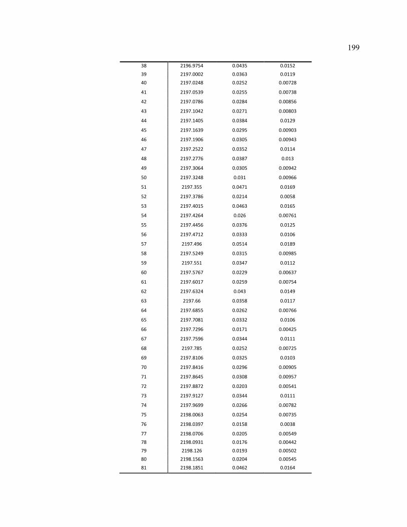
199

38 2196.9754 0.0435 0.0152

39 2197.0002 0.0363 0.0119

40 2197.0248 0.0252 0.00728

41 2197.0539 0.0255 0.00738

42 2197.0786 0.0284 0.00856

43 2197.1042 0.0271 0.00803

44 2197.1405 0.0384 0.0129

45 2197.1639 0.0295 0.00903

46 2197.1906 0.0305 0.00943

47 2197.2522 0.0352 0.0114

48 2197.2776 0.0387 0.013

49 2197.3064 0.0305 0.00942

50 2197.3248 0.031 0.00966

51 2197.355 0.0471 0.0169

52 2197.3786 0.0214 0.0058

53 2197.4015 0.0463 0.0165

54 2197.4264 0.026 0.00761

55 2197.4456 0.0376 0.0125

56 2197.4712 0.0333 0.0106

57 2197.496 0.0514 0.0189

58 2197.5249 0.0315 0.00985

59 2197.551 0.0347 0.0112

60 2197.5767 0.0229 0.00637

61 2197.6017 0.0259 0.00754

62 2197.6324 0.043 0.0149

63 2197.66 0.0358 0.0117

64 2197.6855 0.0262 0.00766

65 2197.7081 0.0332 0.0106

66 2197.7296 0.0171 0.00425

67 2197.7596 0.0344 0.0111

68 2197.785 0.0252 0.00725

69 2197.8106 0.0325 0.0103

70 2197.8416 0.0296 0.00905

71 2197.8645 0.0308 0.00957

72 2197.8872 0.0203 0.00541

73 2197.9127 0.0344 0.0111

74 2197.9699 0.0266 0.00782

75 2198.0063 0.0254 0.00735

76 2198.0397 0.0158 0.0038

77 2198.0706 0.0205 0.00549

78 2198.0931 0.0176 0.00442

79 2198.126 0.0193 0.00502

80 2198.1563 0.0204 0.00545

81 2198.1851 0.0462 0.0164

200

82 2198.2068 0.0223 0.00614

83 2198.239 0.0362 0.0119

84 2198.267 0.0262 0.00767

85 2198.2884 0.0371 0.0123

86 2198.3104 0.0179 0.00452

87 2198.3344 0.0159 0.00385

88 2198.3592 0.0155 0.00372

89 2198.4073 0.0138 0.00313

90 2198.446 0.0368 0.0122

91 2198.4899 0.0148 0.00346

92 2198.5238 0.0267 0.00788

93 2198.5433 0.0113 0.00236

94 2198.56509 0.0117 0.00249

95 2198.58527 0.0153 0.00363

96 2198.624 0.0178 0.00451

97 2198.6421 0.025 0.0072

98 2198.66477 0.0324 0.0102

99 2198.6852 0.0144 0.00333

100 2198.712 0.0161 0.00389

101 2198.744 0.026 0.00758

102 2198.765 0.0154 0.00368

103 2198.782 0.0101 0.002

104 2198.821 0.0155 0.0037

105 2198.864 0.0149 0.00351

106 2198.884 0.0225 0.00621

107 2198.901 0.0155 0.00371

108 2198.932 0.0262 0.00766

109 2198.953 0.012 0.00258

110 2198.975 0.0136 0.00308

111 2199.0186 0.0251 0.00722

112 2199.0572 0.0275 0.0082

113 2199.0854 0.0223 0.00614

114 2199.1105 0.0271 0.00803

115 2199.1373 0.0412 0.0141

116 2199.166 0.0458 0.0162

117 2199.1891 0.0235 0.0066

118 2199.2135 0.0247 0.00706

119 2199.2645 0.0394 0.0133

120 2199.2901 0.0206 0.00549

121 2199.3176 0.0377 0.0126

122 2199.343 0.0407 0.0139

123 2199.3895 0.0389 0.0131

124 2199.4141 0.0309 0.0096

125 2199.4435 0.0396 0.0134

126 2199.4892 0.0373 0.0124

127 2199.5152 0.0253 0.00732

128 2199.5428 0.0273 0.00812

201

129 2199.571 0.032 0.0101

130 2199.5942 0.0157 0.00377

131 2199.6202 0.0179 0.00453

132 2199.6459 0.019 0.00491

133 2199.7043 0.0219 0.00599

134 2199.7295 0.0244 0.00694

135 2199.7667 0.0174 0.00437

136 2199.7912 0.0192 0.00501

137 2199.8173 0.0172 0.00429

138 2199.8471 0.0152 0.00361

139 2199.8729 0.0241 0.00684

140 2199.8949 0.0273 0.00811

141 2199.9176 0.0191 0.00494

142 2199.9529 0.0197 0.00519

143 2199.9708 0.0142 0.00327

144 2200.0104 0.014 0.00319

145 2200.0357 0.00903 0.00171

146 2200.0587 0.0126 0.00275

147 2200.0812 0.0155 0.0037

148 2200.1036 0.00857 0.00159

149 2200.1324 0.0112 0.00232

150 2200.15 0.0153 0.00363

151 2200.1726 0.0105 0.00213

152 2200.2093 0.0139 0.00316

153 2200.234 0.0179 0.00451

154 2200.2598 0.0105 0.00214

155 2200.2809 0.0111 0.00231

156 2200.3298 0.0127 0.00279

157 2200.3691 0.0291 0.00884

158 2200.4126 0.0141 0.00324

159 2200.4378 0.0192 0.00499

160 2200.471 0.0165 0.00405

161 2200.4946 0.021 0.00566

162 2200.5389 0.0207 0.00553

163 2200.5801 0.0198 0.00521

164 2200.6083 0.0356 0.0116

165 2200.6245 0.0209 0.0056

166 2200.6496 0.0238 0.00674

167 2200.6716 0.0221 0.00606

168 2200.6963 0.0299 0.00916

169 2200.7246 0.0292 0.00887

170 2200.749 0.032 0.0101

171 2200.7755 0.019 0.00491

172 2200.8103 0.022 0.00602

173 2200.8613 0.013 0.00289

174 2200.8876 0.0256 0.00742

175 2200.927 0.0228 0.00634

176 2200.9516 0.0306 0.00946

202

177 2200.9765 0.0444 0.0156

178 2201.0068 0.0427 0.0148

179 2201.0359 0.0388 0.013

180 2201.056 0.031 0.00963

181 2201.079 0.0351 0.0114

182 2201.1166 0.0183 0.00467

183 2201.1391 0.0322 0.0101

184 2201.165 0.0353 0.0115

185 2201.2066 0.0295 0.009

186 2201.2315 0.0255 0.0074

187 2201.2587 0.0226 0.00627

188 2201.2856 0.0325 0.0103

189 2201.313 0.0316 0.00988

190 2201.3474 0.0124 0.0027

191 2201.3729 0.0129 0.00287

192 2201.4149 0.0231 0.00645

193 2201.4305 0.0328 0.0104

194 2201.4543 0.0205 0.00545

195 2201.4818 0.0209 0.00562

196 2201.5183 0.0382 0.0128

197 2201.5459 0.0246 0.00703

198 2201.6093 0.0223 0.00613

199 2201.6393 0.022 0.00603

200 2201.6685 0.0191 0.00495

201 2201.6969 0.0302 0.00928

202 2201.7233 0.0333 0.0106

203 2201.7511 0.0312 0.0097

204 2201.7929 0.0482 0.0174

205 2201.8118 0.0276 0.00821

206 2201.839 0.0217 0.00591

207 2201.8638 0.0296 0.00904

208 2201.8939 0.0353 0.0115

209 2201.9221 0.0213 0.00577

210 2201.9686 0.0338 0.0108

211 2201.9951 0.0259 0.00754

212 2202.033 0.0358 0.0117

213 2202.0632 0.0267 0.00787

214 2202.0977 0.0334 0.0107

215 2202.1219 0.0115 0.00243

216 2202.17 0.0323 0.0102

217 2202.1963 0.0213 0.00575

218 2202.2346 0.0375 0.0124

219 2202.2678 0.0168 0.00415

220 2202.3292 0.00874 0.00149

221 2202.3545 0.00607 0.000956

222 2202.3794 0.0119 0.00255

223 2202.4071 0.0144 0.00334

224 2202.4351 0.0114 0.00239

203

225 2202.4614 0.017 0.0042

226 2202.4898 0.0136 0.00308

227 2202.5163 0.0182 0.00465

228 2202.5376 0.0188 0.00485

229 2202.5596 0.0157 0.00377

230 2202.5863 0.0185 0.00476

231 2202.6074 0.00804 0.00145

232 2202.6265 0.00858 0.00159

233 2202.651 0.00822 0.00149

234 2202.6739 0.0109 0.00224

235 2202.7012 0.0127 0.0028

236 2202.7307 0.0126 0.00275

237 2202.7537 0.0127 0.00278

238 2202.7739 0.0197 0.00516

239 2202.7981 0.0289 0.00875

240 2202.8245 0.00988 0.00195

241 2202.8492 0.0163 0.00398

242 2202.8729 0.0134 0.00301

243 2202.8978 0.0142 0.00328

244 2202.9392 0.016 0.00386

245 2202.9675 0.0116 0.00246

246 2202.9959 0.00844 0.00155

247 2203.0251 0.0111 0.00229

248 2203.0504 0.0143 0.0033

249 2203.0753 0.0104 0.00209

250 2203.1013 0.0107 0.00219

251 2203.1262 0.0175 0.00438

252 2203.1553 0.0201 0.00533

253 2203.1844 0.0161 0.00392

254 2203.2104 0.0174 0.00435

255 2203.2353 0.0208 0.00556

256 2203.2605 0.0163 0.00396

257 2203.2838 0.0177 0.00447

258 2203.3147 0.0152 0.00359

259 2203.3428 0.0202 0.00536

260 2203.3712 0.0217 0.00592

261 2203.4044 0.0192 0.00498

262 2203.4334 0.029 0.00882

263 2203.4641 0.0203 0.00539

264 2203.4897 0.0199 0.00524

265 2203.5243 0.027 0.00797

266 2203.5504 0.0245 0.00699

267 2203.5876 0.0291 0.00885

268 2203.6105 0.0172 0.00429

269 2203.6355 0.0295 0.00901

270 2203.6646 0.0281 0.00841

271 2203.7026 0.0162 0.00394

272 2203.7297 0.0314 0.00979

204

273 2203.7589 0.0314 0.0098

274 2203.7841 0.0386 0.0129

275 2203.812 0.0312 0.0097

276 2203.8385 0.0398 0.0135

277 2203.8624 0.0334 0.0107

278 2203.8915 0.0432 0.015

279 2203.923 0.0393 0.0132

280 2203.9494 0.0362 0.0119

281 2203.9744 0.028 0.0084

282 2204.0008 0.0287 0.00866

283 2204.0289 0.0241 0.00682

284 2204.0539 0.0323 0.0102

285 2204.0819 0.0172 0.00427

286 2204.1067 0.0169 0.00418

287 2204.1291 0.0281 0.00843

288 2204.1544 0.0311 0.00966

289 2204.1812 0.0273 0.0081

290 2204.2241 0.0379 0.0126

291 2204.2474 0.0363 0.0119

292 2204.2798 0.026 0.00757

293 2204.3069 0.0193 0.00503

294 2204.3321 0.0161 0.00391

295 2204.3583 0.0213 0.00576

296 2204.3866 0.0207 0.00555

297 2204.415 0.031 0.00964

298 2204.4433 0.0241 0.00685

299 2204.4751 0.0323 0.0102

300 2204.5051 0.0245 0.00699

301 2204.5339 0.0281 0.00843

302 2204.5601 0.0176 0.00444

303 2204.5859 0.0239 0.00677

304 2204.6134 0.0259 0.00753

305 2204.6424 0.0312 0.00971

306 2204.6702 0.0322 0.0101

307 2204.6953 0.0265 0.00777

308 2204.7197 0.0283 0.00853

309 2204.7416 0.0242 0.00686

310 2204.7615 0.0234 0.00657

311 2204.789 0.0158 0.00379

312 2204.8182 0.00938 0.00181

313 2204.8474 0.0133 0.00297

314 2204.8942 0.0138 0.00314

315 2204.9191 0.0164 0.00399

316 2204.9487 0.0161 0.00392

317 2204.9676 0.0166 0.00407

318 2205.0097 0.0278 0.00832

319 2205.0323 0.0163 0.00397

320 2205.062 0.0475 0.017

205

321 2205.088 0.00859 0.00159

322 2205.1157 0.0108 0.0022

323 2205.1423 0.00774 0.00137

324 2205.1701 0.0195 0.00512

325 2205.199 0.026 0.00758

326 2205.2232 0.01 0.00199

327 2205.2467 0.0254 0.00733

328 2205.2726 0.011 0.00229

329 2205.3004 0.0101 0.002

330 2205.3314 0.0212 0.00572

331 2205.3584 0.0146 0.00341

332 2205.3867 0.0235 0.00661

333 2205.4122 0.0194 0.00506

334 2205.4414 0.0173 0.00433

335 2205.4685 0.0264 0.00776

336 2205.4916 0.0173 0.00433

337 2205.524 0.0103 0.00205

338 2205.5493 0.0168 0.00414

339 2205.5917 0.0238 0.00673

340 2205.6199 0.0172 0.00428

341 2205.651 0.0307 0.00952

342 2205.6799 0.0189 0.00489

343 2205.7033 0.0194 0.00506

344 2205.7326 0.0138 0.00315

345 2205.7563 0.0165 0.00403

346 2205.7809 0.0199 0.00526

347 2205.8076 0.0114 0.00239

348 2205.838 0.0163 0.00399

349 2205.8676 0.0228 0.00634

350 2205.8973 0.0196 0.00513

351 2205.9251 0.0254 0.00736

352 2205.9511 0.0248 0.00712

353 2205.9808 0.0253 0.00732

354 2206.0119 0.0271 0.00804

355 2206.0443 0.0193 0.00504

356 2206.0779 0.0296 0.00905

357 2206.1092 0.0306 0.00948

358 2206.1395 0.0336 0.0107

359 2206.1679 0.0333 0.0106

360 2206.1955 0.0294 0.00895

361 2206.2272 0.0307 0.00951

362 2206.2564 0.0325 0.0103

363 2206.2812 0.0309 0.0096

364 2206.3242 0.015 0.00353

365 2206.3456 0.0169 0.00416

366 2206.3771 0.0142 0.00327

367 2206.4067 0.0224 0.00616

368 2206.4354 0.0174 0.00434

206

369 2206.4587 0.0167 0.00411

370 2206.4796 0.00709 0.0012

371 2206.5055 0.0138 0.00315

372 2206.536 0.0165 0.00406

373 2206.5625 0.0179 0.00454

374 2206.5871 0.021 0.00567

375 2206.6161 0.013 0.00288

376 2206.6442 0.0387 0.013

377 2206.6723 0.0365 0.012

378 2206.6968 0.0538 0.0201

379 2206.7253 0.0473 0.0169

380 2206.7501 0.0564 0.0214

381 2206.7766 0.0432 0.015

382 2206.8028 0.0503 0.0184

383 2206.8286 0.0501 0.0183

384 2206.8585 0.0223 0.00616

385 2206.8872 0.0349 0.0113

386 2206.9137 0.0146 0.00342

387 2206.9306 0.0258 0.0075

388 2206.9531 0.0161 0.00392

389 2206.9796 0.0265 0.0078

390 2207.0216 0.00607 0.000957

391 2207.0453 0.0206 0.0055

392 2207.0687 0.0253 0.00732

393 2207.0864 0.0385 0.0129

394 2207.1145 0.0282 0.00848

395 2207.1428 0.0185 0.00473

396 2207.1714 0.0273 0.00809

397 2207.1916 0.0257 0.00747

398 2207.2214 0.024 0.00678

399 2207.2443 0.0172 0.00429

400 2207.2736 0.0143 0.00329

401 2207.3038 0.0135 0.00304

402 2207.3358 0.0113 0.00237

403 2207.3658 0.0168 0.00415

404 2207.3933 0.0205 0.00547

405 2207.4174 0.0287 0.00866

406 2207.4407 0.016 0.00388

407 2207.469 0.014 0.00321

408 2207.4948 0.0271 0.00801

409 2207.521 0.0163 0.00396

410 2207.551 0.0267 0.00788

411 2207.5779 0.0324 0.0102

412 2207.6003 0.0286 0.00862

413 2207.623 0.0308 0.00957

414 2207.6456 0.0318 0.00997

415 2207.6677 0.0298 0.00912

416 2207.6925 0.0244 0.00695

207

417 2207.7442 0.026 0.0076

418 2207.7686 0.0325 0.0103

419 2207.7961 0.0326 0.0103

420 2207.8187 0.013 0.00289

421 2207.8484 0.0313 0.00977

422 2207.8771 0.0396 0.0134

423 2207.9044 0.0216 0.00589

424 2207.937 0.0171 0.00425

425 2207.9656 0.032 0.0101

426 2207.992 0.0441 0.0154

427 2208.0204 0.0351 0.0114

428 2208.0575 0.038 0.0127

429 2208.0819 0.0273 0.00812

430 2208.1091 0.0211 0.0057

431 2208.1548 0.0393 0.0132

432 2208.1795 0.0264 0.00777

433 2208.207 0.0295 0.00901

434 2208.2381 0.0283 0.0085

435 2208.2675 0.0213 0.00578

436 2208.2962 0.0316 0.00988

437 2208.3343 0.0198 0.00521

438 2208.3856 0.0346 0.0112

439 2208.4152 0.0263 0.0077

440 2208.4622 0.0176 0.00441

441 2208.4868 0.0202 0.00537

442 2208.5145 0.022 0.00602

443 2208.54 0.0322 0.0101

444 2208.5653 0.023 0.00642

445 2208.5882 0.0132 0.00295

446 2208.6159 0.0202 0.00536

447 2208.6459 0.0171 0.00424

448 2208.6751 0.0101 0.00202

449 2208.706 0.00887 0.00167

450 2208.7536 0.0096 0.00187

451 2208.7836 0.0228 0.00635

452 2208.8152 0.0202 0.00535

453 2208.8438 0.00951 0.00184

454 2208.8714 0.013 0.0029

455 2208.9179 0.0125 0.00275

456 2208.9477 0.0103 0.00208

457 2208.9878 0.0238 0.00672

458 2209.0304 0.0259 0.00756

459 2209.0569 0.0239 0.00676

460 2209.0851 0.0258 0.00751

461 2209.1182 0.0368 0.0121

462 2209.1647 0.028 0.0084

463 2209.1948 0.0271 0.00802

464 2209.2207 0.0196 0.00514

208

465 2209.2524 0.02 0.00531

466 2209.2841 0.0158 0.00382

467 2209.3184 0.0153 0.00364

468 2209.3523 0.0285 0.00861

469 2209.3789 0.0122 0.00264

470 2209.4149 0.0117 0.00247

471 2209.4567 0.0113 0.00237

472 2209.4877 0.0119 0.00254

473 2209.5398 0.0181 0.00461

474 2209.5705 0.0243 0.00693

475 2209.6 0.026 0.00758

476 2209.6614 0.0351 0.0114

477 2209.6905 0.0118 0.00252

478 2209.7504 0.0179 0.00453

479 2209.7912 0.00949 0.00184

480 2209.8207 0.0134 0.00301

481 2209.8543 0.0154 0.00367

482 2209.8993 0.011 0.00229

483 2209.9467 0.0205 0.00547

484 2209.9771 0.023 0.0064

485 2210.0264 0.0319 0.01

486 2210.0622 0.029 0.0088

487 2210.0806 0.0362 0.0119

488 2210.109 0.0279 0.00833

489 2210.1462 0.0102 0.00204

490 2210.1708 0.0127 0.00279

491 2210.1956 0.026 0.00761

492 2210.2217 0.0281 0.00842

493 2210.2469 0.0199 0.00526

494 2210.2939 0.0296 0.00908

495 2210.3247 0.0164 0.004

496 2210.3575 0.0252 0.00729

497 2210.3884 0.0195 0.00511

498 2210.4209 0.00818 0.00148

499 2210.479 0.0142 0.00328

500 2210.5267 0.0107 0.0022

501 2210.556 0.0154 0.00367

502 2210.588 0.0267 0.00786

503 2210.6305 0.011 0.00226

504 2210.6592 0.0259 0.00755

505 2210.6884 0.0134 0.00299

506 2210.7209 0.0248 0.00712

507 2210.7522 0.0189 0.00488

508 2210.7854 0.0233 0.00654

509 2210.8287 0.0156 0.00372

510 2210.8569 0.0168 0.00415

511 2210.8886 0.0179 0.00452

512 2210.9276 0.0269 0.00792

209

513 2210.9545 0.025 0.00718

514 2210.9807 0.0101 0.00201

515 2211.0119 0.0116 0.00247

516 2211.0435 0.0105 0.00211

517 2211.0744 0.0184 0.0047

518 2211.1081 0.0209 0.0056

519 2211.1603 0.0137 0.00312

520 2211.1802 0.0173 0.00432

521 2211.2067 0.0104 0.00211

522 2211.2357 0.00955 0.00185

523 2211.2651 0.0219 0.00601

524 2211.2969 0.0258 0.0075

525 2211.3242 0.0202 0.00534

526 2211.3575 0.0197 0.00519

527 2211.379 0.0194 0.00507

528 2211.3994 0.0167 0.00409

529 2211.4202 0.0146 0.00338

530 2211.456 0.00827 0.00151

531 2211.5072 0.00799 0.00143

532 2211.5368 0.017 0.0042

533 2211.5673 0.0114 0.00239

534 2211.6004 0.0292 0.00889

535 2211.6257 0.0285 0.00859

536 2211.6479 0.0164 0.00402

537 2211.671 0.0186 0.00477

538 2211.6921 0.0357 0.0116

539 2211.7245 0.0291 0.00882

540 2211.7576 0.0163 0.00396

541 2211.793 0.0159 0.00383

542 2211.8236 0.0177 0.00445

543 2211.8527 0.0252 0.00726

544 2211.8892 0.0189 0.00488

545 2211.9277 0.014 0.00319

546 2211.9566 0.0196 0.00512

547 2211.9901 0.0151 0.00356

548 2212.0227 0.0144 0.00335

549 2212.0435 0.0207 0.00554

550 2212.0613 0.0155 0.00368

551 2212.0845 0.0271 0.008

552 2212.1283 0.015 0.00355

553 2212.1544 0.0189 0.00489

554 2212.2028 0.0226 0.00625

555 2212.2454 0.0192 0.005

556 2212.2717 0.0124 0.0027

557 2212.2983 0.00979 0.00192

558 2212.3151 0.0121 0.0026

559 2212.3381 0.0103 0.00207

560 2212.3628 0.0218 0.00596

210

561 2212.3886 0.0203 0.0054

562 2212.4448 0.0246 0.00703

563 2212.4891 0.0284 0.00855

564 2212.5145 0.0172 0.00427

565 2212.5434 0.0261 0.0076

566 2212.5678 0.0152 0.00361

567 2212.597 0.022 0.00603

568 2212.6199 0.0193 0.00501

569 2212.6485 0.0122 0.00263

570 2212.6833 0.0211 0.00568

571 2212.7082 0.0246 0.00702

572 2212.7347 0.0194 0.00508

573 2212.7592 0.00882 0.00165

574 2212.7846 0.0178 0.00447

575 2212.8318 0.0237 0.00669

576 2212.8522 0.0299 0.00919

577 2212.8895 0.0202 0.00537

578 2212.912 0.0282 0.00848

579 2212.9472 0.0224 0.00618

580 2212.9751 0.026 0.00758

581 2213.006 0.0283 0.0085

582 2213.0362 0.0275 0.00816

583 2213.0647 0.0193 0.00503

584 2213.09 0.0159 0.00382

585 2213.1119 0.0235 0.00661

586 2213.1363 0.0235 0.00661

587 2213.1601 0.0204 0.00542

588 2213.2285 0.0163 0.00397

589 2213.2523 0.0137 0.00312

590 2213.3131 0.0255 0.00739

591 2213.371 0.0133 0.00298

592 2213.3958 0.0272 0.00808

593 2213.4211 0.0362 0.0119

211

APPENDIX D. Ambient and Pulse-Decay for 10 core-plugs of Porosity and Permeability

Measurements, Well 13-12-78-11W6

Sample Depth m

Lab Hydrostatic Confining Pressure

kPa

Reservoir Confining Pressure

kPa

Porosity fraction

Air Permeability mD

1 2196.1164 Ambient 0.086086962 0.0070823

14465.71 25467.7993 0.079821893 0.0055316

4 2197.7081 Ambient 0.079341539 0.0033024

6667.465 11738.49472 0.074834766 0.0028746

10583.825 18633.49472 0.0728435 0.0026993

14465.71 25467.7993 0.07122656 0.0024288

18416.545 32423.49472 0.06987149 0.0022101

22332.905 39318.49472 0.068760133 0.0019024

26249.265 46213.49472 0.067834631 0.0016571

5 2198.57 Ambient 0.062526467 0.0011819

6667.465 11738.49472 0.05695228 0.0010527

10583.825 18633.49472 0.05456139 0.0009146

14465.71 25467.7993 0.052655458 0.0007486

18416.545 32423.49472 0.051084979 0.000648

22332.905 39318.49472 0.049817252 0.0005262

26249.265 46213.49472 0.048777404 0.0004524

7 2199.89 Ambient 0.060249753 0.0011392

14465.71 25467.7993 0.054162562 0.0006265

10 2201.84 Ambient 0.070798702 0.0023603

14465.71 25467.7993 0.06502505 0.0016511

12 2203.08 Ambient 0.059155857 0.000703

14465.71 25467.7993 0.053720415 0.0003558

16 2206.75 Ambient 0.086691563 0.0081566

14465.71 25467.7993 0.080303134 0.0060151

20 2209.46 Ambient 0.043056168 0.0004686

14465.71 25467.7993 0.038177911 0.0001364

212

Sample Depth m

Lab Hydrostatic Confining Pressure

kPa

Reservoir Confining Pressure

kPa

Porosity fraction

Air Permeability mD

24 2212.98 Ambient 0.056220473 0.0014687

6667.465 11738.49472 0.052997437 0.0013456

10583.825 18633.49472 0.05157517 0.0012422

14465.71 25467.7993 0.050420989 0.0010995

18416.545 32423.49472 0.049454167 0.001012

22332.905 39318.49472 0.04866147 0.0008981

26249.265 46213.49472 0.048001451 0.0008145

25 2213.4 Ambient 0.068382977 0.0101828

14465.71 25467.7993 0.063031054 0.009571

Documents

Characterizing reservoir properties for the lower triassic