Stephanie L. Shaw (EPRI), Stephen F. Mueller, Qi Mao, Ray Valente, and John Mallard (Tennessee Valley Authority)

20th International EPA Emission Inventory Conference

August 13-16, 2012

Fugitive Emissions from a Dry Coal Fly Ash Storage Pile

2 © 2012 Electric Power Research Institute, Inc. All rights reserved.

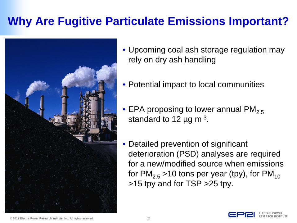
Why Are Fugitive Particulate Emissions Important?

• Upcoming coal ash storage regulation may rely on dry ash handling

• Potential impact to local communities

• EPA proposing to lower annual PM2.5 standard to 12 µg m-3.

• Detailed prevention of significant deterioration (PSD) analyses are required for a new/modified source when emissions for PM2.5 >10 tons per year (tpy), for PM10 >15 tpy and for TSP >25 tpy.

3 © 2012 Electric Power Research Institute, Inc. All rights reserved.

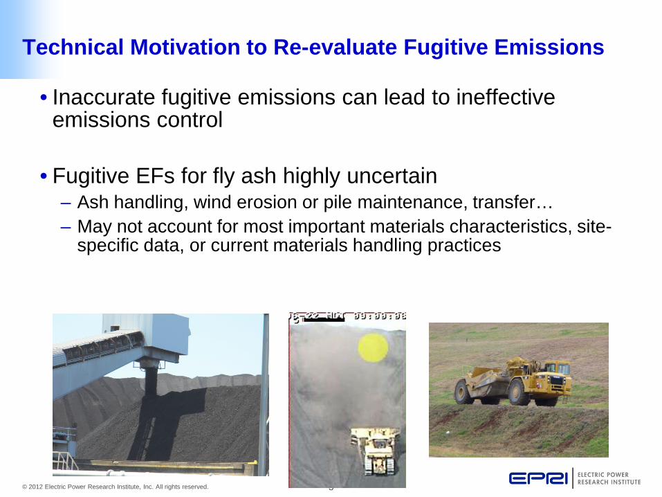
Technical Motivation to Re-evaluate Fugitive Emissions

• Inaccurate fugitive emissions can lead to ineffective emissions control

• Fugitive EFs for fly ash highly uncertain – Ash handling, wind erosion or pile maintenance, transfer… – May not account for most important materials characteristics, site-

specific data, or current materials handling practices

4 © 2012 Electric Power Research Institute, Inc. All rights reserved.

Overall Study Plan

• Phase 1: Dry fly ash– TVA Colbert Plant (AL) 1200MW • Phase 2: Coal dust – TVA Gallatin Plant (TN) 1000MW • Phase 3: TBD - Limestone/gypsum? Road dust? Fly ash in Western U.S.?

5 © 2012 Electric Power Research Institute, Inc. All rights reserved.

Project Goals

• Quantify fugitive particulate emissions at coal-fired power plants for different handling practices.

• Compare new emission rates with those from EPA AP-42 handbook.

• Utilities use to inform facility permitting.

• May help evaluate emission mitigation strategies

6 © 2012 Electric Power Research Institute, Inc. All rights reserved.

Origins of AP-42 Fugitive Emission Factors

• Studies in 1970s measured airborne dust near unpaved roads and material handling. Multi-component statistical analyses to develop formulations. Dropping factors -1980s

• Used old measurement technologies. • Most sources were staged & not done under actual

operating conditions. • Involved limited types of materials & limited range in

conditions (vehicle speed, material moisture content, silt content).

7 © 2012 Electric Power Research Institute, Inc. All rights reserved.

bscat Ash handling

Dumping ≈25 m3 per load

Leveling to 0.5 m high x 4 m dia.

Grading time ≈8 min

Grader speed ≈5 mph

Loads per hr = ≤12

road dust

Study Concept

0 20 40 60

5 15

25

35

45

55

65

75

85

>90

%

Conc., µg/m3

PMc PM2.5

8 © 2012 Electric Power Research Institute, Inc. All rights reserved.

Colbert Field Study Layout

Fly ash

disposal area

N

102 m

56 m

Potential

source

location

Photos:

(Top) Camera triggered by trucks moving along berm road south of air monitoring sites.

(Bottom) Camera triggered by activity on fly ash dry stack. 8 20 m high

9 © 2012 Electric Power Research Institute, Inc. All rights reserved.

Monitoring Instrumentation

Instrument Measurement/Purpose Met One beta attenuation monitors (BAMs) at downwind & background sites

PM2.5/PM10 concentrations (semi-continuous) @ downwind & background sites

BGI PQ-200 PM10 particle filter sampler Filtered PM10 sample, ~12-hr samples (for chemical analysis) @ downwind & background sites

TSI 3563 3-λ nephelometer Continuous βscat @ 3 wavelengths @ downwind site

Optek nephelometer Semi-continuous single-wavelength βscat @ downwind site

Campbell Scientific video camera Semi-continuous images of fly ash disposal site

Instrument Measurement/Purpose R. M. Young 81000RE sonic anemometers (2 & 10 m)

Wind speed, direction, vertical velocity, horizontal & vertical turbulence; vertical gradient of speed, direction & turbulence

Vaisala HMI41 aspirated temperature & humidity sensors (2 & 10 m)

Air temperature & relative humidity; vertical temperature & moisture gradients

Campbell Scientific CNR2 net radiometer (~1.8 m) Radiation flux (shortwave, longwave & net)

Novalynx Corp. 260-2501-A tipping bucket raingage

Precipitation amount

Campbell Scientific CS616 water content reflectometer (top 30 cm of soil)

Soil moisture content

Met

eoro

logi

cal

Air

Qua

lity

10 © 2012 Electric Power Research Institute, Inc. All rights reserved.

Dry Fly Ash Handling at Colbert

• Fly ash is pneumatically conveyed to hoppers where it is conditioned with 15% moisture before transference to haul trucks.

• Each truck moves 25-28 m3 of ash per load. • Ash is dropped at disposal area and leveled to a depth of

about half a meter (18-24 in). • Ash grading takes about 8 min with grader moving at 2.2

m s-1 (5 mph). • Fugitive emissions are primarily due to dropping and

grading operations (haul trucks moving over bottom ash road produces very little fugitive dust).

11 © 2012 Electric Power Research Institute, Inc. All rights reserved.

Average Particulate Concentrations by Direction May-August 2011

One-hr average concentrations were measured by FRM BAMs and reported here in µg m-3.

Wind direction was measured at a height of 10 m.

(3) (2)

Data recovery >99%

Data recovery 81% Data recovery >99%

12 © 2012 Electric Power Research Institute, Inc. All rights reserved.

Hourly Concentrations at each Site: May-September 2011

13 © 2012 Electric Power Research Institute, Inc. All rights reserved.

Clean Period (No Emissions) 28 June, 1300-1400 LST

0

10

20

30

40

50

60

06/2

8/20

11 1

3:00

06/2

8/20

11 1

3:02

06/2

8/20

11 1

3:04

06/2

8/20

11 1

3:06

06/2

8/20

11 1

3:08

06/2

8/20

11 1

3:10

06/2

8/20

11 1

3:12

06/2

8/20

11 1

3:14

06/2

8/20

11 1

3:16

06/2

8/20

11 1

3:18

06/2

8/20

11 1

3:20

06/2

8/20

11 1

3:22

06/2

8/20

11 1

3:24

06/2

8/20

11 1

3:26

06/2

8/20

11 1

3:28

06/2

8/20

11 1

3:30

06/2

8/20

11 1

3:32

06/2

8/20

11 1

3:34

06/2

8/20

11 1

3:36

06/2

8/20

11 1

3:38

06/2

8/20

11 1

3:40

06/2

8/20

11 1

3:42

06/2

8/20

11 1

3:44

06/2

8/20

11 1

3:46

06/2

8/20

11 1

3:48

06/2

8/20

11 1

3:50

06/2

8/20

11 1

3:52

06/2

8/20

11 1

3:54

06/2

8/20

11 1

3:56

06/2

8/20

11 1

3:58

06/2

8/20

11 1

4:00

B_sc

at

20110628_13:00-14:00

14 © 2012 Electric Power Research Institute, Inc. All rights reserved.

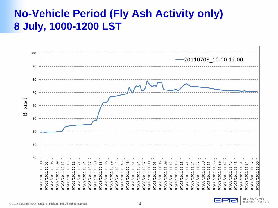
No-Vehicle Period (Fly Ash Activity only) 8 July, 1000-1200 LST

20

30

40

50

60

70

80

90

100

07/0

8/20

11 1

0:00

07/0

8/20

11 1

0:03

07/0

8/20

11 1

0:06

07/0

8/20

11 1

0:09

07/0

8/20

11 1

0:12

07/0

8/20

11 1

0:15

07/0

8/20

11 1

0:18

07/0

8/20

11 1

0:21

07/0

8/20

11 1

0:24

07/0

8/20

11 1

0:27

07/0

8/20

11 1

0:30

07/0

8/20

11 1

0:33

07/0

8/20

11 1

0:36

07/0

8/20

11 1

0:39

07/0

8/20

11 1

0:42

07/0

8/20

11 1

0:45

07/0

8/20

11 1

0:48

07/0

8/20

11 1

0:51

07/0

8/20

11 1

0:54

07/0

8/20

11 1

0:57

07/0

8/20

11 1

1:00

07/0

8/20

11 1

1:03

07/0

8/20

11 1

1:06

07/0

8/20

11 1

1:09

07/0

8/20

11 1

1:12

07/0

8/20

11 1

1:15

07/0

8/20

11 1

1:18

07/0

8/20

11 1

1:21

07/0

8/20

11 1

1:24

07/0

8/20

11 1

1:27

07/0

8/20

11 1

1:30

07/0

8/20

11 1

1:33

07/0

8/20

11 1

1:36

07/0

8/20

11 1

1:39

07/0

8/20

11 1

1:42

07/0

8/20

11 1

1:45

07/0

8/20

11 1

1:48

07/0

8/20

11 1

1:51

07/0

8/20

11 1

1:54

07/0

8/20

11 1

1:57

07/0

8/20

11 1

2:00

B_sc

at

20110708_10:00-12:00

15 © 2012 Electric Power Research Institute, Inc. All rights reserved.

3-Vehicle Event 22 July, 0700-0800 LST

30

40

50

60

70

80

90

100

110

07/2

2/20

11 7

:00

07/2

2/20

11 7

:02

07/2

2/20

11 7

:04

07/2

2/20

11 7

:06

07/2

2/20

11 7

:08

07/2

2/20

11 7

:10

07/2

2/20

11 7

:12

07/2

2/20

11 7

:14

07/2

2/20

11 7

:16

07/2

2/20

11 7

:18

07/2

2/20

11 7

:20

07/2

2/20

11 7

:22

07/2

2/20

11 7

:24

07/2

2/20

11 7

:26

07/2

2/20

11 7

:28

07/2

2/20

11 7

:30

07/2

2/20

11 7

:32

07/2

2/20

11 7

:34

07/2

2/20

11 7

:36

07/2

2/20

11 7

:38

07/2

2/20

11 7

:40

07/2

2/20

11 7

:42

07/2

2/20

11 7

:44

07/2

2/20

11 7

:46

07/2

2/20

11 7

:48

07/2

2/20

11 7

:50

07/2

2/20

11 7

:52

07/2

2/20

11 7

:54

07/2

2/20

11 7

:56

07/2

2/20

11 7

:58

07/2

2/20

11 8

:00

B_sc

at

20110722_07:00-08:00

1 2

3

All three dust spikes were caused by dump trucks on the berm road.

16 © 2012 Electric Power Research Institute, Inc. All rights reserved.

Particle Concentrations (SSE-SSW)

y = 0.225x + 1.854 R² = 0.770

0

10

20

30

40

0 20 40 60 80 100 120 140

µg m

-3

Mm-1

PM2.5 Concentration vs. bscat

y = -0.014x2 + 6.432x - 2.745 R² = 0.725

1

10

100

1000

0 10 20 30 40 50 60 70

µg m

-3

Mm-1

PMc Conc. vs. σbscat

17 © 2012 Electric Power Research Institute, Inc. All rights reserved.

Models of Hourly PMc & PM2.5

Ccoarse=fσσbscat + fU2U2 + ffineCfine + Cint r2=0.77

Multivariate linear regression yields

Cfine=fbscatbscat + fU2U2 + Cint r2=0.89

f : regression slope constants

bscat : light scattering coefficient (Mm-1)

σscat : standard deviation of bscat (Mm-1)

U2 : wind speed at level 2 (m s-1 @10 m)

Cint : intercept constants (µg m-3)

Cfine : concentration of PM2.5 mass (µg m-3)

Ccoarse : concentration of PMc mass (µg m-3)

18 © 2012 Electric Power Research Institute, Inc. All rights reserved.

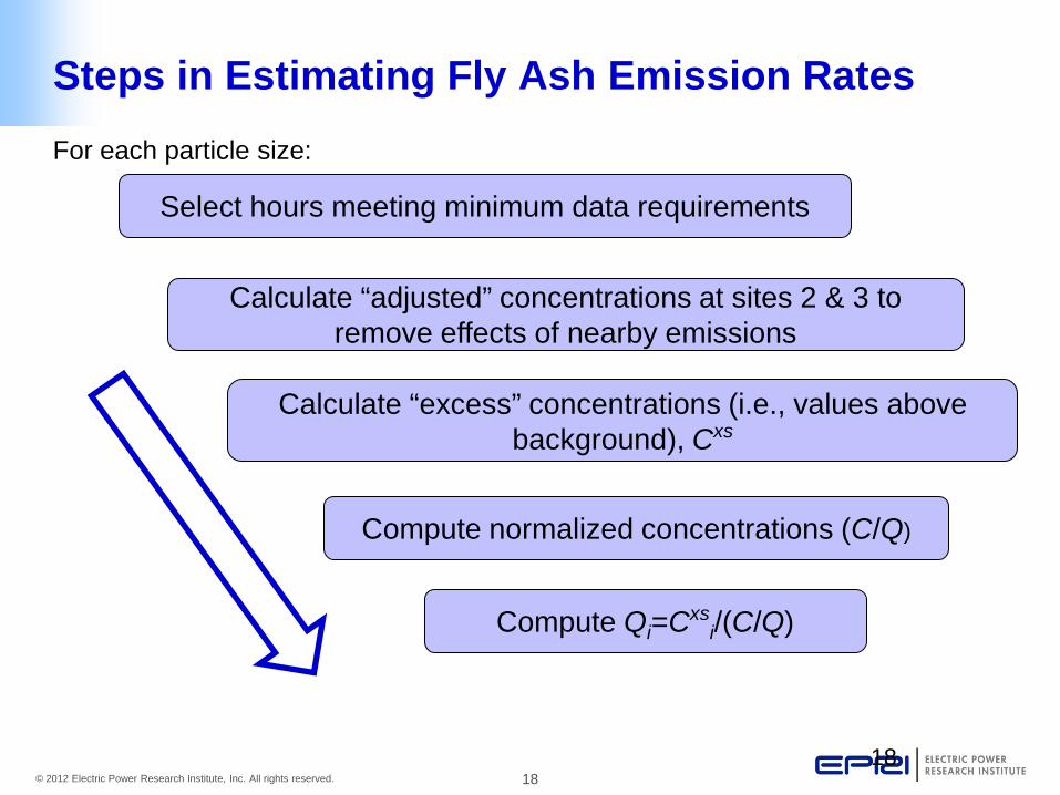
Steps in Estimating Fly Ash Emission Rates

18

Select hours meeting minimum data requirements

Calculate “adjusted” concentrations at sites 2 & 3 to remove effects of nearby emissions

Calculate “excess” concentrations (i.e., values above background), Cxs

Compute normalized concentrations (C/Q)

Compute Qi=Cxsi/(C/Q)

For each particle size:

19 © 2012 Electric Power Research Institute, Inc. All rights reserved.

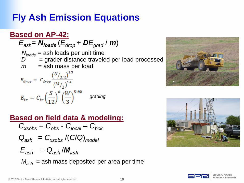
Fly Ash Emission Equations

Based on AP-42: Eash= Nloads (Edrop + DEgrad / m)

Nloads = ash loads per unit time D = grader distance traveled per load processed m = ash mass per load

Based on field data & modeling:

Cxsobs = Cobs - Clocal – Cbck

Qash = Cxsobs /(C/Q)model

Eash = Qash /Mash Mash = ash mass deposited per area per time

grading

20 © 2012 Electric Power Research Institute, Inc. All rights reserved.

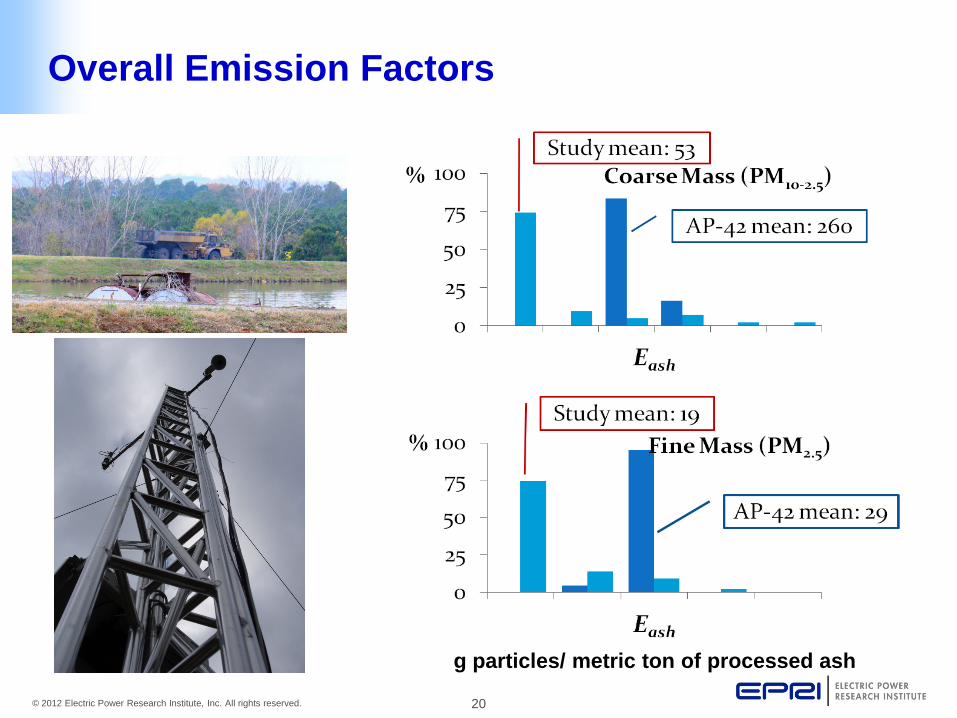
Overall Emission Factors

g particles/ metric ton of processed ash

21 © 2012 Electric Power Research Institute, Inc. All rights reserved.

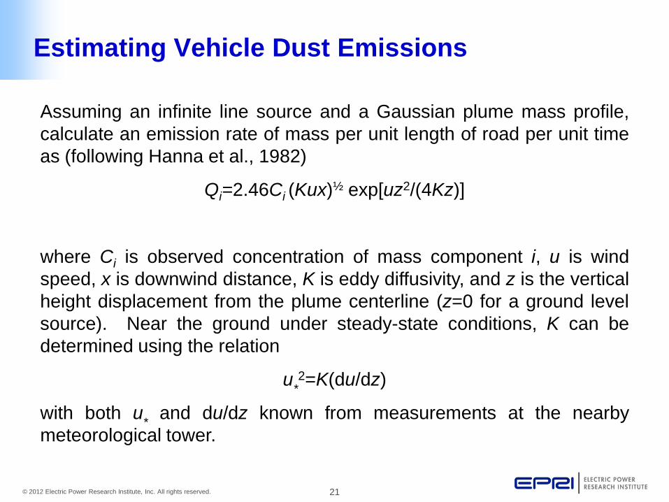
Estimating Vehicle Dust Emissions

Assuming an infinite line source and a Gaussian plume mass profile, calculate an emission rate of mass per unit length of road per unit time as (following Hanna et al., 1982)

Qi=2.46Ci (Kux)½ exp[uz2/(4Kz)]

where Ci is observed concentration of mass component i, u is wind speed, x is downwind distance, K is eddy diffusivity, and z is the vertical height displacement from the plume centerline (z=0 for a ground level source). Near the ground under steady-state conditions, K can be determined using the relation

u*2=K(du/dz)

with both u* and du/dz known from measurements at the nearby meteorological tower.

22 © 2012 Electric Power Research Institute, Inc. All rights reserved.

Emission Factor Summaries

Emission Factor Coarse Mass, PMc Fine Mass, PM2.5 Mean Median Mean Median

Fly Ash, AP-42 (g PM per Mg ash) 250 232 45 41

Fly Ash, this study (g PM per Mg ash) 63 12 14-18 5-7

Road dust, AP-42 - industrial sfc. (g PM per km traveled) 193 200 34 36

Road dust, AP-42 - public roads (g PM per km traveled) 32 26 5.7 4.6

Road dust, this study (g PM per km traveled) 68e 38e 3.3 1.4

23 © 2012 Electric Power Research Institute, Inc. All rights reserved.

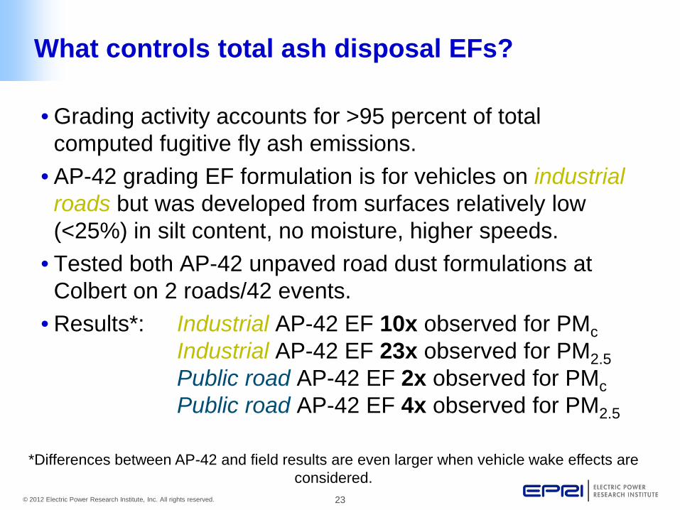
What controls total ash disposal EFs?

• Grading activity accounts for >95 percent of total computed fugitive fly ash emissions.

• AP-42 grading EF formulation is for vehicles on industrial roads but was developed from surfaces relatively low (<25%) in silt content, no moisture, higher speeds.

• Tested both AP-42 unpaved road dust formulations at Colbert on 2 roads/42 events.

• Results*: Industrial AP-42 EF 10x observed for PMc Industrial AP-42 EF 23x observed for PM2.5 Public road AP-42 EF 2x observed for PMc Public road AP-42 EF 4x observed for PM2.5

*Differences between AP-42 and field results are even larger when vehicle wake effects are considered.

24 © 2012 Electric Power Research Institute, Inc. All rights reserved.

Conclusions • Despite conservative assumptions, AP-42 derived fly ash handling EFs are higher

than EFs derived by field measurements for both PMc and PM2.5 • Disparity is likely due to high bias in industrial unpaved road dust formulation

(grading).

• EFs from field measurements have higher tail than AP-42 EFs. May be due to higher variability in atmospheric or ash handling conditions in real operations.

• Use of more realistic EFs can lower fugitive dust emission estimates for fly ash handling by 33% (PM2.5) to 80% (PM10). Can benefits be expanded to TSP?

• Observed EFs for vehicles on unpaved roads also differ from AP-42 EFs.

25 © 2012 Electric Power Research Institute, Inc. All rights reserved.

Together…Shaping the Future of Electricity