Embed Size (px)
Citation preview

CHARACTERIZATION OF WEAK ROPE THROUGH THE
DESIGN AND CONSTRUCTION OF A PORTABLE TENSILE TESTING MACHINE
BY
GLENN MCGILLICUDDY B.S. Mechanical Engineering, University of New Hampshire, 2001
THESIS
Submitted to the University of New Hampshire In partial fulfillment of
The Requirement for the Degree of
Master of Science
In
Ocean Engineering
December 2005

This thesis has been examined and approved.
_________________________________ Thesis Director, Kenneth C. Baldwin Professor of Mechanical and Ocean Engineering _________________________________ Lloyd C. Huff Research Professor of Center for Coastal And Ocean Mapping _________________________________ Scott Kraus Vice President for Research, New England Aquarium _________________________________ Yuri Rzhanov Research Associate Professor of Center For Coastal and Ocean Mapping
_______________ Date

iii
DEDICATION
To my family, friends, and colleagues.

iv
ACKNOWLEDGEMENTS This work is a result of research sponsored in part by the New England
Aquarium and the National Ocean and Atmospheric Administration, U.S. Department
of Commerce under grant number: 14N372 through the University of New Hampshire.
I would like to take this opportunity to thank the following people for their
support throughout this project. To Paul Lavoie, thank you for your engineering and
fabrication support for which the project depended on. To Dr. Lloyd Huff, for his
endless knowledge on every topic encountered for the duration of the project (and then
some) and for giving me direction when the correct path seemed to be unclear.
Appreciation is extended to Dr. Yuri Rzhanov as well, for his video image processing
techniques in extracting the high resolution elongation data. To Dr. Ken Baldwin,
thank you for your guidance as a graduate advisor and for providing feedback and
revisions on this work. To Dr. Barbara Kraft, thank you for answering countless
Matlab questions and providing direction to appropriate data processing techniques.
To Dr. Scott Kraus, a thanks for the background insight as to why the project is
important and the years of knowledge of whale behavior and entanglements. Thanks
to Jud DeCew, Chad Turmelle, and Glen Rice for the splicing lessons, the occasional
helping hand, and reality checks. To Dr. Norm Holy and Bob Ames of Seaside Inc.,
thank you for the development of WSR and providing a sample for testing. Last but
not least, to the whole of CCOM, especially Director Larry Mayer, for providing the

v
facilities and the flexibility in the daily work schedule to complete this milestone in
my education. I am greatly in debt to you all. Thank you.

vi
TABLE OF CONTENTS DEDICATION ............................................................................................................. iii
ACKNOWLEDGEMENTS ......................................................................................... iv
LIST OF TABLES ....................................................................................................... ix
LIST OF FIGURES ...................................................................................................... x
NOMENCLATURE...................................................................................................xiii
ABSTRACT................................................................................................................ xv
CHAPTER I: INTRODUCTION................................................................................. 1
1. Background ................................................................................................. 1
2. Goals / Objective......................................................................................... 5
3. Approach..................................................................................................... 5
CHAPTER II: CORDAGE INSTITUTE GUIDELINES ............................................ 7
CHAPTER III: MACHINE DESIGN ........................................................................ 10
1. General ...................................................................................................... 10
2. Mechanical ................................................................................................ 14
3. Hydraulics ................................................................................................. 26
CHAPTER IV: FABRICATION ............................................................................... 33
1. Part Specification ...................................................................................... 33
2. Assembly................................................................................................... 36
3. Apparatus Testing and Modification......................................................... 39
CHAPTER V: INSTRUMENTATION ..................................................................... 44

vii
1. General System Overview......................................................................... 44
2. Measurement System Error Analysis........................................................ 48
3. Instrument Calibrations............................................................................. 52
CHAPTER VI: ROPE TESTING .............................................................................. 57
1. Experimental Design................................................................................. 57
2. Procedure .................................................................................................. 60
CHAPTER VII: DATA PROCESSING .................................................................... 69
1. General ...................................................................................................... 69
2. Video Data Processing .............................................................................. 70
3. Matlab Data Processing ............................................................................ 73
CHAPTER VIII: RESULTS AND DISCUSSION.................................................... 76
1. General ...................................................................................................... 76
2. Physical Properties .................................................................................... 78
3. Engineering Properties .............................................................................. 80
CHAPTER IX: CONCLUSIONS .............................................................................. 86
REFERENCES............................................................................................................ 89
APPENDICIES ........................................................................................................... 91
APPENDIX A: DESIGN CALCULATIONS............................................................ 92
APPENDIX B: AUTOCAD FABRICATION DRAWINGS .................................. 106
APPENDIX C: MATLAB CODE ........................................................................... 122
APPENDIX D: ENGINEERING STRESS-STRAIN PLOTS................................. 140
APPENDIX E: FIRST DERIVATIVE OF STRESS WITH RESPECT TO TIME............... 144

viii
APPENDIX F: SECOND DERIVATIVE OF STRESS WITH RESPECT TO TIME.......... 148

ix
LIST OF TABLES Table 3.1: Location of centroids for the composite beam.......................................... 23
Table 3.2: Estimated weight of apparatus components.............................................. 25
Table 3.3: Hydraulic piston characteristics................................................................ 29
Table 3.4: Estimated hydraulic losses and heat generation........................................ 32
Table 5.1: Calculated measurement uncertainties...................................................... 52
Table 7.1: Input arguments for RopeMovie program ................................................ 72
Table 8.1: Strands remaining after breaking .............................................................. 76
Table 8.2: Location of breaks within the center section ............................................ 77
Table 8.3: Physical properties .................................................................................... 78
Table 8.4: Physical expected mean estimate error ..................................................... 79
Table 8.5: Engineering properties .............................................................................. 81
Table 8.6: Engineering expected mean estimate error ............................................... 84
Table A.1: Anchor pin calculation results.................................................................. 95

x
LIST OF FIGURES Figure 1.1: Vertical buoy line weak link...................................................................... 3
Figure 1.2: Gill net weak link ...................................................................................... 3
Figure 3.1: Flow chart of the design process ............................................................. 10
Figure 3.2: Scissor design concept............................................................................. 11
Figure 3.3: Custom Cordage testing apparatus .......................................................... 12
Figure 3.4: Hydraulic design concept ........................................................................ 13
Figure 3.5: AutoCAD drawing of the UNH testing apparatus................................... 15
Figure 3.6: Free body diagram of an anchor plate ..................................................... 19
Figure 3.7: Cross section of the structural members.................................................. 23
Figure 3.8: Structural member free body diagram..................................................... 24
Figure 3.9: UNH wave tank hydraulic power pack.................................................... 26
Figure 3.10: Schematic of the testing apparatus’s hydraulic circuit .......................... 28
Figure 4.1: Assembly drawing showing the placement of the thrust plate ................ 37
Figure 4.2: Assembly drawing of the crosshead ........................................................ 38
Figure 4.3: Original method for securing the load cell .............................................. 40
Figure 4.4: Modified stationary anchorage ................................................................ 41
Figure 4.5: Fray location in relation to thimble ......................................................... 42
Figure 4.6: Yarn comparison .................................................................................... 42
Figure 5.1: Block diagram showing data flow........................................................... 45

xi
Figure 5.2: Gauge mark placement ............................................................................ 47
Figure 5.3: Crosshead speed calibration setup........................................................... 53
Figure 5.4: Calibration plot for crosshead speed ....................................................... 54
Figure 5.5: Bridgesensor calibration setup ................................................................ 55
Figure 5.6: Calibration curve for the bridgesensor .................................................... 55
Figure 5.7: Final calibration curve for the load cell bridgesensor setup.................... 56
Figure 6.1: Student’s t-distribution ............................................................................ 59
Figure 6.2: Setup for determining Physical properties .............................................. 61
Figure 6.3: Masking used during black stripe application ......................................... 63
Figure 6.4: Masking used during white stripe application......................................... 64
Figure 6.5: Saltwater soak.......................................................................................... 65
Figure 6.6: Setup for determining Engineering properties ........................................ 65
Figure 7.1: Front panel for Lens Correct program..................................................... 71
Figure 8.1: Comparison plot for dry and wet WSR engineering properties .............. 82
Figure 8.2: Comparison plot for polypropylene and dry WSR engineering properties............ 83
Figure D.1: Engineering Stress-Strain of WSR-Dry................................................ 141
Figure D.2: Engineering Stress-Strain of WSR-Wet ............................................... 141
Figure D.3: Engineering Stress-Strain Comparison of Wet and Dry WSR ............. 142
Figure D.4: Engineering Stress-Strain of Polypropylene......................................... 142
Figure D.5: Engineering Stress-Strain Comparison of WSR-Dry and Polypropylene............ 143
Figure E.1: First Derivative of Stress for WSR-Dry................................................ 145
Figure E.2: First Derivative of Stress for WSR-Wet ............................................... 145
xii
Figure E.3: First Derivative of Stress Comparison of Wet and Dry WSR .............. 146
Figure E.4: First Derivative of Stress for Polypropylene......................................... 146
Figure E.5: First Derivative of Stress Comparison of WSR-Dry and Polypropylene ............ 147
Figure F.1: Second Derivative of Stress for WSR-Dry ........................................... 149
Figure F.2: Second Derivative of Stress for WSR-Wet ........................................... 149
Figure F.3: Second Derivative of Stress Comparison of Wet and Dry WSR .......... 150
Figure F.4: Second Derivative of Stress for Polypropylene .................................... 150
Figure F.5: Second Derivative of Stress Comparison of WSR-Dry and Polypropylene ........ 151

xiii
NOMENCLATURE A: Cross-sectional Area As: Cross-sectional Area at Maximum Stress B: Unit Measure for Width of the Confidence Interval c: Unit of Measure from the Centroid d: Unit Measure for Diameter E: Young’s Modulus of Elasticity f: Friction Factor F: Applied Force F’: Primary Shear Force F”: Secondary Shear Force g: Gravitational Constant hl: Head Loss I: Area Moment of Inertia ITp: Initial Tension per CI Guidelines Kt: Stress Concentration Factor l: Unit Measure for Length LDp: Linear Density per CI Guidelines M: Moment Mmax: Maximum Bending Moment n: Number of Samples NA: Neutral Axis Nr: Reynolds Number P: Pressure Phyd: Hydraulic Horsepower Pn: Pressure Drop across the component specified by n Q: Hydraulic Flow Rate r: Unit Measure for Radius RTp: Reference Tension per CI Guidelines Sg: Specific Gravity of Hydraulic Oil t: Unit Measure for Thickness V: Transverse (Shear) Force or Hydraulic Fluid Velocity Vmax: Maximum Transverse (Shear) Force w: Unit Measure for Width x : Centroidal X-Axis Distance from the Origin y : Centroidal Y-Axis Distance from the Origin ymax: Maximum Deflection zα/2: Z-statistic

xiv
α: Form Factor based on Cross-sectional Area ∆P: Pressure Drop β: Angle between Primary and Secondary Shear Forces γH2O: Specific Weight of Water ν: Kinematic Viscosity θmax: Deflection Angle of a Beam σ: Tangential Stress and Statistical Standard Deviation σmax: Maximum Tangential Stress σo: Nominal Normal Stress τ: Transverse (Shear) Stress τmax: Maximum Transverse (Shear) Stress

xv
ABSTRACT
CHARACTERIZATION OF WEAK ROPE THROUGH THE DESIGN AND CONSTRUCTION OF A
PORTABLE TENSILE TESTING MACHINE
by
Glenn McGillicuddy
University of New Hampshire, December, 2005 The North Atlantic Right Whale (NARW) is considered to be one of the
world’s most endangered whale species. Dr. Scott Kraus of the New England
Aquarium extensively reviewed the available data and concluded that although
ship/whale collisions are more deadly than entanglements it is entanglements that
happen more frequently and should raise concern (Kraus 1990). Whale Safe Rope
(WSR) has been developed on the premise that a whale collision with the fixed fishing
gear using WSR will cause a localized point of high stress and the WSR will
theoretically break at the point of impact.
This study involves the design and construction of an apparatus for evaluating
the characteristics of WSR, as well as, the development of a robust experimental
methodology for future evaluations of WSR or similar rope. Video image processing
and typical data acquisition techniques were employed. This lead to precise
engineering stress-strain curves being developed for the WSR and standard
polypropylene rope. The engineering stress-strain curves of WSR indicate that the

xvi
WSR exhibited properties that more closely match that of a brittle material when
compared to engineering stress-strain curves of standard polypropylene. Statistical
analysis of the data supported the conclusion that the experimental methodology was
robust. The results of this experimental test, as well as the development of the fixture
and methodology, will allow future researchers and end-users of small size rope/line to
better understand the behavior of the most common piece of equipment which impacts
cost and safety in the marine industry. That is to say, rope.

1
CHAPTER I
INTRODUCTION 1. Background The North Atlantic Right Whale (NARW Eubalaena glacialis), is considered
to be one of the world’s most endangered whale species. Prior to the introduction of
whaling, NARW was believed to be numbered in the thousands. The large decline in
past years is attributed to whaling, although the NARW has not made a significant
recovery since its placement on the endangered species list in 1936.
In response to the repeated endangerment and neglect of marine mammals the
United States established the Marine Mammal Protection Act (MMPA) in 1972. The
act put a moratorium on all marine mammal products, foreign and domestic, to further
prevent the exploitation of marine mammals and to conserve them for future
generations.
However despite these efforts, the growth rate of the NARW in recent years
has been declining such that it is predicted that the NARW will likely become extinct
in the year 2190 (Caswell, Fujiwara, and Brault 1999). Three factors which have been
identified as major contributors to the troubled status of the NARW are: (1) water
quality, (2) ship collisions, and (3) entanglements in fixed fishing gear. Kraus (Kraus
1990) extensively reviewed the available data and concluded that although ship/whale

2
collisions are more deadly than entanglements, it is entanglements that occur more
frequently.
Of the known fifty plus deaths of NARWs between 1970 and 2001, nine
percent were a direct result of entanglements in fishing gear (Knowlton and Kraus
2001). Over seventy percent of the present NARW population exhibit signs of past
entanglements. More importantly, the number of potentially fatal and fatal
entanglements has risen in recent years (Cavatorta et al. 2003). Cavatorta concluded
that fixed traps and gill nets, as well as, the vertical buoy lines pose the most serious
class of entanglement hazard.
The Atlantic Large Whale Take Reduction Plan (ALWTRP) was established in
response to the growing negative trend in the well-being of all large whales. The first
stage of ALWTRP, which went into effect in 1997, restricted where and when
commercial fixed fishing gear can be deployed. In February 1999, ALWTRP further
dictated requirements on rigging and deployment methods of commercial fixed fishing
gear in these restricted areas by introducing the weak link concept.
The weak link concept in commercial fixed fishing rigging consists of a weak
element which is designed to fail in the event that a whale collides with the gear or
somehow becomes entangled with the gear. The weak element is placed on the
vertical buoy lines, specifically where the buoy is tied to the upper end of the vertical
line (Figure 1.1).

3
Figure 1.1: Weak link connecting surface buoy and hauling line (a.k.a. vertical buoy line weak
link). Photograph courtesy of NOAA Bulletin: “Techniques for Making Weak Links and Marking Buoy Lines”.
The reasoning behind placing the link there is that the buoy will break away thereby
allowing the line to slip through the mouth of the whale, free from any obstructions,
i.e. knots. Weak links are also incorporated into the float lines and net panels of the
commercial gill net rigs, as seen in figure 1.2.
Figure 1.2: Weak link installed in a gill net panel. Note the knot in the weak link to reduce the breaking strength of the weak link. Photograph courtesy of NOAA Bulletin: “Techniques for
Making Weak Links and Marking Buoy Lines”.
Although this is a huge step forward in rigging fixed fishing gear in order to
improve the safety of all marine mammals, there still exist problems with these
methods. The first problem being that obstacles remain attached to the line after the
weak link fails and can act as points that add to the friction already experienced by the

4
rope in contact with the animal. These obstructions come in many shapes and forms
that include but, are not limited to, intact weak links, knots used in weak links, splices
(eye and/or end to end), and anything else that may be attached below the weak link
which alters (increases) the overall diameter of the line used.
In an attempt to alleviate this problem, Dr. Norm Holy and Bob Ames of
Seaside, Inc. developed a product called Whale Safe Rope (WSR). WSR is a
polypropylene based rope with varying amounts of barium sulfate mixed into the
polymer chain to control (reduce) the breaking strength of the rope. WSR was
developed to avoid the difficulties with discrete weak links. Deploying WSR in all the
rigging lines would eliminate the need for discrete weak links because the rigging
itself is a continuous weak link. The intended advantage of using WSR is that when a
large whale collides with the fixed fishing gear the resulting localized point of high
stress will break there rather than at a weak link device that may be some distance
away from the point of impact. The theoretical risk of entanglement in the line goes
down due to the fact the animal would not be dragging anything that may get wrapped
around any body appendages on the whale.
The exact interactions between large whales and fixed fishing gear are
unknown because none have been observed. An effort is presently underway at the
University of New Hampshire (UNH) in cooperation with the New England Aquarium
(NEAq) to study the potential interactions between large whales and fixed fishing gear
in the water column on a model scale. It is suggested that when the entanglement
process is understood it will be evident that WSR is a viable alternative to the present
combination of discrete weak link and line. This study involves determining the

5
engineering properties of WSR in order to better characterize it for modeling purposes.
The WSR characteristics will be compared to 3/8” standard polypropylene line that is
commonly used by the fixed fishing gear industry.
2. Goals / Objectives The specific goals of this research are:
1) Research and gather appropriate technical material to conduct the following tests on the WSR:
a. Physical Properties i. Reference Tension
ii. Initial Tension iii. Size Number iv. Linear Density
b. Engineering Properties i. Uncycled Strength (Breaking Strength)
ii. Uncycled Strain
2) Design and construct a portable low cost rope testing apparatus to test not only dry rope specimens but also specimens that have been soaked in salt water.
3) Develop the methodology and verify the degree of robustness through the
analysis of experimental data. Robustness was defined in two parts: a. The ability of the testing apparatus to perform without deflections or
malfunctions and the measurement systems to provide consistent, accurate results.
b. The ability of test to be preformed by an average person without specialized training and obtain high quality and high precision results.
4) Characterize WSR for the UNH effort in modeling whale-gear interactions.
5) Compare WSR to the commercial fixed fishing industry standard 3/8”
polypropylene rope. 3. Approach
A critical need exists for the ways and means to evaluate varying kinds of rope,
specifically Whale Safe Rope, in order to justify potential modifications to fishing

6
gear and in order to establish a basis for ongoing whale-gear research at UNH Ocean
Engineering. This study focuses on the evaluation of WSR through the development
of a testing apparatus for use in the laboratory and, if necessary, in the field. In March
2004, the Fifth International Rope Technology Workshop was attended. This
provided a working knowledge of terminology, testing procedures, and the
acknowledged authorities in the field of tension member research. As a compliment to
the knowledge gained in the work shop, the Cordage Institute (CI) through its
technical references provided detailed guide lines and valuable insights into the
principals of manufacturing, testing, and application.
The information gained from the workshop and from the CI influenced the
design of the rope testing apparatus. The design hinged on the general design
specifications provided by Seaside, Inc. as well as the suggested testing methods of the
CI and the criterion set forth by the UNH initiative. Construction began in August
2004. The rope testing apparatus which in the end underwent a series of preliminary
evaluation tests followed by modifications, produced acceptable and repeatable breaks
of the WSR.
After the apparatus was demonstrated to produce consistent acceptable breaks,
an evaluation was conducted on the process. The evaluation verified the manufacture’s
load cell calibration and calibrated the cross head travel velocity. These two
calibration processes ensured a known baseline for the subsequent rope testing.
A comparison of the WSR and traditional 3/8” polypropylene line, as tested on
the rope testing apparatus, was made to determine what were the notable differences
beyond the obvious difference in ultimate breaking strength.

7
CHAPTER II
CORDAGE INSTITUTE GUIDELINES The Cordage Institute (CI) was founded in 1920 and is composed of
manufactures and sellers of cordage, rope, and twine. The institute developed and
published, in 1980, the first known testing standards for fiber ropes. The American
Society for Testing Materials (ASTM) produced standards three years later which
were revised in 1989. It is widely accepted that the CI’s methods are the industry
standards (Flory 1997). The CI revised their testing method guidelines in the early
1990’s and again in 2002. The guidelines produced by the CI are so widely accepted
nationally and internationally that ASTM withdrew their guidelines in June of 2002
(ASTM 1993). The CI guide lines that were followed during this study.
Several of the CI guidelines were essential to the design process which
includes test specimen length, force application rate, strain rate, and minimum
measurement accuracies. Compliance with these basic standards is essential to
produce industry accepted results.
Specimen length plays a vital role in the design of the UNH rope testing
machine because it defines not only the minimum distance between attachment points
but also the dynamic range that the specimen must be stretched to break. The institute
specifies two specimen sizes that are based on the overall diameter of the rope being
tested. If the sample is less then 5/8” then the required length between gauge marks is

8
one foot. For any sample over 5/8” the required length between gauge marks is six
feet. The CI also requires that there be two gauge marks which are simply non-
intrusive marks placed as reference points on the rope under test. Given that the WSR
has a manufacturer specified nominal diameter of 3/8”, this study used a one foot
measure between gauge marks. In addition to the distance between gauge marks, the
CI also specifies that there must be at least one-half foot clearance at each end of the
gauge marks before the terminations to the testing apparatus occur. Consequently the
minimum specimen length is two feet.
The application of force to the specimen under a breaking force test is also
regulated by the institute, but not as stringently. The CI states that during testing, the
time allowed for the specimen to be loaded to 20% of its estimated breaking force
must be in the range of two to two hundred seconds. Having established the speed for
the loading, it must be maintained throughout the test in order to provide a constant
and uniform strain rate. The speed for the loading helps identify the hydraulic
specifications discussed in the following chapter.
Lastly, the Cordage Institute specifies minimum accuracies for all force,
length, and weight measuring instrumentation. The force measurements must be
accurate to ± 5% of the calculated reference tension unless an elongation/extension
test is done. If the elongation test is to be completed, the required tolerance on
accuracy is ± 1%. The length and changes of length must be accurately measured to ±
1/16”. The measurement accuracy for the weight of a specimen must be measured to
an accuracy of ±0.25% of the total specimen weight. All these measurement systems

9
must have calibrations that are traceable, well documented, and conducted within one
year of the date of the rope testing.
These criterion set forth by the CI are crucial to obtaining test results that are
acceptable within the industry. The design, construction, and evaluation of the rope
testing machine were conducted in a manner that was consistent with the CI criterion.

10
CHAPTER III
MACHINE DESIGN 1. General The design process followed a traditional mechanical engineering design
process as outlined below in figure 3.1.
Figure 3.1: Flow chart of the design process employed during the design portion of the project.
The recognition of need and problem definition were clearly outlined in the
introduction chapter. The third, fourth, and fifth steps, which include synthesis,
analysis and optimization, and evaluation, are the discussion in this chapter.

11
The guidelines of the Cordage Institute were used as a basis for establishing a
set of design criterion for the development of the UNH rope testing apparatus. The
three categories were established for the design. They were mechanical, hydraulic,
and instrumentation and were governed by CI guidelines for specimen size, force
application rate, and measurement accuracies, respectively.
Working within these guidelines, a series of three initial design concepts were
investigated. The three conceptual designs for the apparatus were called scissor,
capstan, and hydraulic ram.
In the first design called scissor, it was conceptualized as having two strength
members, probably constructed from steel box beam, that were pinned together at their
centers. At one end, the two strength members would be linked via a hydraulic piston.
At the opposite end of the scissor, the specimen under test would be mounted. The
scissor concept is visualized in the conceptual drawing presented as figure 3.2.
Figure 3.2: Scissor design concept (backing plate not shown).

12
A structural plate for mounting the entire scissor is not shown in figure 3.2. The
structural backing plate would serve to constrain the device to actions in one plane of
motion. During testing, the hydraulic piston would be extended thus applying a
tension force to the specimen. The idea of this design is that it could be secured to a
dock with the structural members extending into the water to conduct tests while the
rope specimen was under water. However, initial calculations indicated that the
apparatus would be too bulky to meet a portable criterion. Furthermore considerable
complexity of moving parts would be needed to constrain the scissor to one plane of
action.
The second design, called capstan, was considered after a field visit to Custom
Cordage of Waldoboro Maine. Custom Cordage possessed a similar apparatus to that
shown, figure 3.3, which was used to conduct quality assurance tests when producing
cordage for government institutions.
Figure 3.3: Custom Cordage testing apparatus for quality assurance testing.
A specimen would be secured to the load cell by taking a few wraps around a drum
attached to the load cell. The other end of the specimen would be wrapped around the

13
rotating drum of the capstan and allowed to accumulate on the drum thus applying a
tension force to the specimen. This concept had several drawbacks. When observing
tests being conducted with their apparatus it was noted that the specimen would
continually settle on the drum of the capstan as the tension was gradually increased
until the specimen broke. It was recognized that the continual settling actually
violates the Cordage Institute guidelines CI 1500-02:9.4.2 and CI 1500-02:9.4.3,
which state that once a test is in progress the strain rate must continue at the same rate
at which it started.
The third design, hydraulic ram, consisted of a combination of the two
previous designs. The conceptual design consisted of a structural member with a fixed
anchorage at one end and a moving anchorage in the opposite one-third of the
structural member (Figure 3.4).
Figure 3.4: Hydraulic design concept.
A hydraulic ram would provide the driving force for the moving anchorage. The rope
member under test would be placed between the anchorages and a tensile force applied

14
by the ram. The only foreseeable drawback to this system was the cost associated
with the hydraulic power pack needed to actuate the system.
The third conceptual design was eventually chosen over the other two designs.
The mechanical category which initially took into account the specimen size was
expanded to include other issues like portability, maximum design load, specimen
behavior, and specimen mounting. The hydraulic category was also expanded to
include limitations. In addition to the rate of force application, these limitations
included specifications on several in-house preexisting hydraulic power packs. As
with the other two categories, the instrumentation design category was expanded to
include additional parameters above and beyond the guidelines laid out by the
Cordage Institute. Based on these additional design considerations, a series of design
iterations were completed prior to construction of the UNH testing apparatus. The
final design evaluation is outlined in the following Mechanical and Hydraulic sections.
2. Mechanical
The fundamental objective of this apparatus is simple: break the specimen of
rope that is under test. However, interactions between all of the mechanical parts must
be understood to confidently conclude that a test will be adequately conducted and that
the measurements acquired will truly represent the conditions undergone by the
specimen. The general components of the tensile testing apparatus are illustrated in
figure 3.5.

15
Figure 3.5: Final AutoCAD drawing of the UNH test apparatus showing the various parts. Note
that the hydraulic piston is hidden inside between the C-channels.
The mechanics of the UNH testing apparatus can be broken down further by starting
with the specimen under test, progressing on to the specimen anchor points, then to the
anchorages, followed by the transmission of force to the main structural member (the
backbone of the apparatus), and finally to the portable supporting structure.
As previously stated, the specimen length must have a minimum length
between the terminations. However, the CI specifications do not describe the type or
length of the end terminations. For example when eye splices are used as specimen
terminations, great care must be taken in choosing the angle at which the working end
re-enters the running end of the rope. Typically in a thimble, this angle is in the
neighborhood of 20 degrees off the centerline of the rope for a total spread of about 40
degrees. Also, the number of tucks must be sufficient to not cause a stress
concentration in the specimen. A general rule of thumb suggests that the number of
tucks must be at least five although no scientific evidence was found to validate this.

16
Another option for the specimen end terminations would be to take a couple of wraps
around a drum and mechanically pinch the end such that the drum reduces the force to
zero at this point. However, this allows the specimen to continually settle during the
test which is in violation of the CI’s guidelines as mentioned earlier. For this
reasoning it was decided to terminate the specimen with eye splices.
The length of the specimen was crucial to sizing the design of the testing
apparatus. The amount of elongation that occurs before the rope actually breaks was
important because the apparatus needed to be designed with a limited amount of
throw. Review of the various rope compounds indicated that nylon exhibits the
greatest elongation under tension. Three-eighths inch three strand nylon, for example,
has a 15% stretch at 30% of its ultimate breaking strength, which is around two tons
(Sampson 2003). This suggests that if a three-foot specimen were used that it would
elongate 5.5” at 30% of its ultimate breaking strength, not including any settling of the
terminations. On this basis, the maximum specimen length was established at three
feet and the apparatus was expected to have a working tension of 5000 pounds with a
throw of at least one foot.
The design tension was set at 5000 lbs however the hydraulics (which are
discussed in 3. Hydraulics) are capable of producing roughly three times that force. A
second set of calculations were preformed, and thus the design revised to include this
factor of safety to the system
Once the length and terminations of the specimen were considered, the design
work turned to securing the specimen using eye splices. It was decided to secure the
specimen using a simple pin mounted in the anchorages. The pins would have to

17
withstand the design tension of 5000 pounds. The pins must not only sustain this
tension force but must also have a small deflection.
The anchor pins were considered as rigidly fixed ended circular beams with a
single force applied to the midpoint of the span. Based on Roark’s formulas for stress
and strain (Young 1989), the maximum bending moment (Mmax), maximum transverse
shear (Vmax), and maximum deflection (ymax) on the anchor pins are represented by the
following expressions:
8maxlFM ⋅
= at 2l (1)
2maxFV = when F is at
2l (2)
IElFy⋅⋅
⋅−=
192
3
max at 2l (3)
where F is the load (Force), l is the point of application of the force from an end, E is
Young’s Modulus of Elasticity, and I is the area moment of inertia about the centroidal
axis of the beam’s cross section. From general mechanics (Beer and Johnson 1996)
the maximum bending moment and the maximum transverse shear equations can be
written as follows for the maximum tangential stress (σmax) and the maximum
transverse (shear) stress (τmax):
IcM ⋅
= maxmaxσ (4)
AVmax
max ⋅= ατ (5)

18
where c is the maximum distance from the neutral axis, α is the form factor of the
cross section (typically equal to 4/3 for a cylindrical cross section), and A is the cross
sectional area.
Calculations for the pins were made for various cross sectional sizes and
lengths for loads of 5000 lbs and 15000 lbs. The calculations are tabulated, in
Appendix A. In the final design, a one-inch diameter by six-inch long, W1 tool steel
was chosen for the anchor pins. This decision was based on the factor of safety of
about 1.5 between the tangential stress and the yield stress at the design load. The fact
that the theoretical deflection of the anchor pin was only four thousandths of an inch
was influential in concluding the final design sizes and material.
The anchor pins tie into what is known as the anchor plates, shown in figure
3.5. These anchor plates must secure the pins such that minimal movement is allowed.
The anchor plates must also withstand and transfer the forces produced during the test
to the structural member of the apparatus. The anchor plate connections must be made
to minimize any deflections by the apparatus’s structural components that would
falsify the results. Stress calculations to determine the appropriate size of the
anchorages were conducted, using the coordinate system presented in the free body
diagram of figure 3.6.

19
Figure 3.6: Free Body Diagram (not to scale) of the anchor plate illustrating the applied force (F) and the resulting forces on the bolt pattern (A, B, C, D). The callout shows the convention used
for determining the shear loading on each individual bolt.
The initial stress calculation used a fixed plate with the design load acting
along the x-axis or tangential of the plane of the plate. General thin-plate theory
would have been applied in this case except that the assumption that the load is
applied normal to the midsurface plane would have been violated. The flexure of
straight bars can not be used because the span to height ratio (the width of the plate) in
this case, is less than eight which violates a basic assumption of beam theory.
Therefore, a geometric approach was taken (Frocht and Hill 1940) to compensate for
the stress concentration of a one-inch hole in the anchorage plate that must
accommodate the anchor pin. The stress concentration factor for the normal (Kt)
stress can be written:
otK
σσmax= (6)
where σmax is the maximum normal stress, and σo is the nominal normal stress. The
stress concentration factor is obtained by interpolating a graph of stress concentration
20
factors versus the dimensionless ratio of the hole diameter (d) to width of the plate
(w). The nominal stress is defined as follows:
( ) tdwF
o ⋅−=σ (7)
where t is the thickness of the plate. Once the nominal stress and the stress
concentration factor are known, equation (6) can be solved for the maximum stress
experienced based solely on the geometric properties of the hole in the plate.
Next, the forces were examined at the connection of the anchor plates to the
structural backbone of the apparatus. This connection is made by a pattern of bolts.
The bolt pattern that secures the anchor plates was investigated for failure in pure
shear loading, bearing stress, and critical bending stress of the bolted plate (Shigley
and Mischke 1989).
Figure 3.6 illustrates the name convention given to the bolt pattern along with
the centroid of the bolt pattern (O) and the convention used for examining the shear
load of the individual bolts. The centroid is the point at which the moment reaction is
about and the shear reaction would pass through. Thus, the primary shear load (F’),
also known as the direct load, can be written:
nVF =' (8)
where n is the number of bolts in the bolt group. The loading on each bolt due to the
moment, called the secondary shear load (F”), can also be written:
DCBA
n
rrrrrMF⋅⋅⋅
⋅=" (9)

21
where r is the radial distance between the centroid and the bolt center. Since the
geometry is symmetric in both axes, the secondary shear forces are the same and can
be written:
rMF⋅
=4
" (10)
Through the introduction of the parallelogram rule, as seen in the call out of figure 3.6
the two vectors (F’ and F”) can be added to yield the resultant load (Fn) on each
respective bolt.
)cos"'2("' 22nn FFFFF β⋅⋅⋅++= (11)
where βn is the angle between F’ and F”. This shows the bolts that are closest to the
point of application of the load experience the greatest force, in this case bolts A and
B.
The bolts used to connect the anchor plates to the structural members of the
apparatus are flat hex head countersunk bolts of size 3/8” – 16 x 1” composed of
Grade 5 steel. Since these bolts come fully threaded, the maximum shear stress will
be applied over the minor pitch diameter of the treads. By American National
Standards Institute (ANSI) standards, the area at this location (As) is 0.0678 in2 and the
maximum bolt shear stress can be written:
s
AorB
AF
=maxτ (12)
Since the thickness of the web (tw) of the c-channel used for the structural members of
the apparatus is thinner than the thickness of the anchor plates (t), the largest bearing
stress will occur where the bolt presses against the web of the c-channel. Based on the

22
American Standard Channel parameters, the bearing stress (σbear) can be calculated
using the general stress equation with the area equal to:
wboltbear tdA ⋅= (13)
The critical bending stress was calculated through the bolts A and B, where the stress
is the greatest. The results of this calculation should be viewed as an approximation
due the assumption that the anchor plate is indeed a bar, which as discussed earlier,
violates beam theory. Equation (5) is employed with the second moment of area
obtained by the implementation of the transfer formula:
( )AdIII holesbar ⋅+⋅−= 22 (14)
where d is the horizontal distance between the bolt pattern centroid and the bolt center.
“A” in equation (14) is the bearing area between the bolt and the anchor plate.
After these calculations were completed, a comparison was made to determine
which element of the anchor plate would fail first, the stress concentration due to
anchor pin hole or the shearing of the bolts due to the eccentric loading. The result
was that the bolt group will fail prior to failure due to the stress concentration
produced by the hole for the anchor pin. Similar, calculations were also made for the
moving cross head attached to the hydraulic piston. In addition to ensuring that the
bolts securing the stationary anchorage would not fail, the aforementioned set of
calculations were utilized to determine the load rating of bearings needed in the cross
head.
When the analysis of the anchor plates was complete, attention was moved
onto the analysis of the backbone or structural members of the apparatus. The main
structural member of the apparatus is actually composed of two C6 x 10.5 C-channels

23
with a top plate, 0.5” thick and 6” wide. As shown in the cross section depicted in
figure 3.7, those items are bolted such as to create a 6.5” x 6” semi-closed U-channel.
Figure 3.7: Cross section of the structural members in relation to the anchor plates.
The numbering convention used for calculations assigned a #1 to the top plate, a #2 to
the left hand C-channel, and a #3 to the right hand C-channel. The coordinate origin is
located in the lower left corner of the composite with a right hand positive sign
convention, as seen figure 3.7. The overall length of the apparatus was set at eight feet
in part to accommodate potential future work on larger specimens in both the length
and diameter dimension. The centroid of the cross-sectional geometry of the
composite, was determined and tabulated in table 3.1.
Table 3.1: Location of centroids for the composite beam.
Area xbar ybar xbarA ybarA(in 2 ) (in) (in) (in 3 ) (in 3 )
1 3.000 3.000 6.250 9.000 18.7502 3.090 0.499 3.000 1.542 9.2703 3.090 5.501 3.000 16.998 9.270
Sums 9.180 N/A N/A 27.540 37.290
First moments of the component areas
Component

24
The position of the neutral axis was computed using the lower left corner of the
composite as the origin:
∑∑=
AAx
x (15)
∑∑=
AAy
y (16)
The next step was to calculate the moment of inertia (I1,2,3) for each of the components
and sum all the components to achieve the moment of inertia (I) for the composite
beam. Using both the maximum force output of the hydraulics and the design force
based on the tensile strength of the cordage, the maximum (Mmax) and design (Mdesign)
moments were calculated respectively.
The principal of superposition was then applied to the length of the composite
beam such that it could be divided into two equal halves as seen in figure 3.8.
Figure 3.8: Structural member free body diagram. Illustration showing the analysis technique to
determine the stress and deflections of the test apparatus's structural members.
25
This allows for each half section to be represented as a member loaded by a
concentrated intermediate moment. Furthermore, the boundary conditions of a fixed
end can be applied at the end where the full length beam was cut in half and a free end
can be applied at the ends of the full length beam. This is possible because in the
middle of the full length beam, the deflection angle is zero and the moment is zero.
The worst case scenario for the two equal halves is when the moment is applied at the
free end, so these are the conditions that define the calculations. The deflection
magnitude (ymax) and deflection angle (θmax) are represented by the equations:
IElMy⋅⋅⋅
=2
2max
max (17)
IElM
⋅⋅−
= maxmaxθ (18)
where l is the length of the half composite beam. Equation (4) can also be applied at
this point substituting the location of the neutral axis (ybar) for “c” to yield the stress in
the composite.
A table of weights was constructed as the final phase of the design analysis on
the mechanical elements of the UNH apparatus.
Table 3.2: Table of weights for mechanical components only.
Calculated Weight Number Needed Total Weight(lb) (lb)
Anchor Pin 1.61 4 6.42Anchor Plate 13.82 2 27.64Cross Head Plate 15.79 2 31.58Thrust Plate 22.56 1 22.56Top Plate 81.22 1 81.22C-channel 84 2 168
Grand Total (lb) 337.42
Estimated weight of apparatus componentsComponent

26
This indicates that the legs which support the apparatus must support about 340 lbs,
not including any of the hydraulic parts. It was decided to construct the legs at a 45
degree angle to offer the most support against tipping and to place scaffolding casters
under the legs so that it can easily be rolled around. The structural members were also
place at a height above the floor such that the bottom edge was relatively the same
height of a standard pickup truck bed for ease of transportation to a remote site. The
attention to mechanical design and the sizing of critical elements that are subject to
stress was important to achieve the mechanical aspect of robustness.
3. Hydraulics
The Jere A. Chase Ocean Engineering Laboratory houses a variety of hydraulic
equipment. The largest being the custom power pack for the Tow/Wave tank wave
generator pictured below.
Figure 3.9: Hydraulic Power Pack used for the generation of waves in the Jere A. Chase Ocean Engineering Laboratory. Note the placement of the selector valve installed to switch between
wave generation and power take off (PTO) circuit.

27
This power pack has a maximum flow capacity of 19.8 gallons per minute (GPM) at a
maximum output pressure of 5000 psi. The adjustable pressure relief valve is
currently set at 1950 psi with an inline accumulator with a pressure setting of 650 psi.
The hydraulic horsepower (Phyd) produced by a power pack (Cundiff 2002) is written:
1714QPPhyd⋅
= (19)
where P in psi is the output pressure and Q in GPM is the flow rate. In this case the
power pack is capable of generating 22.5 hp at the current settings or 57.7 hp at
maximum capacity. Although it constituted a violation of the portability goal, it was
decided to use this power pack for the actuation of the UNH rope testing apparatus.
The decision was largely based on economics. If portability becomes a major issue
then a different power pack will be required.
It was purposed to modify the current setup, by incorporating a power take off
(PTO) point. This would create a point where by the rope testing apparatus’s
hydraulic circuit could be connected and disconnected with ease. The selection
between the wave generation circuit and the PTO is accomplished using what is
known as a selector valve, marked by the letter “A” in figure 3.10.
28
Figure 3.10: Schematic showing the rope testing apparatus’s hydraulic circuit and the insertion of
the selector valve to create a PTO point.
When the PTO circuit is selected via the selector valve, hydraulic power is transmitted
through quick disconnects (B) into flexible hydraulic hoses (C) to the apparatus were
an identical set of quick disconnects are located. The hydraulic fluid then flows to a
directional control valve (D) to control the actuation direction of the hydraulic piston
(G). The allowable actuation direction can be either extend, contract, or neutral.
Beyond the directional control valve (DCV), a load check valve (E) was placed to
prevent the hydraulic piston from moving when the DCV is in the neutral position.
Since the Cordage Institute specifies a constant strain rate, a flow control valve (F) is
placed in-line with the line that supplies hydraulic pressure to the extension of the
hydraulic cylinder.
To determine the implications of this circuit on the operation of the hydraulic
power pack, a theoretical analysis was conducted (Cundiff 2002) of the expected
requirements and losses for pressure, flow, and the amount of heat production. A
piecewise approach was taken to analyze the circuit starting with the requirements of
the hydraulic piston. As stated before, the travel rate of the hydraulic cylinder must

29
remain constant throughout the test. It was decided that the rate should be 144 inches
per minute. Multiplying the flow rate by the surface area of the hydraulic piston
yields a flow rate of hydraulic fluid to move the piston at the desired velocity. The
pressure output from the power pack required to produce the design tension on the
specimen was found by dividing the required tension by the surface area of the piston.
These calculations were made for various piston surface areas and are tabulated below.
Table 3.3: Table of varying piston surface areas and the required flow rates and pressure inputs.
Velocity Diameter Surface Area Flow Rate(in/min) (in) (in 2 ) (gal./min) Design (psi) Maximum (psi)
1 0.79 0.49 6366.2 19098.591.5 1.77 1.1 2829.42 8488.262 3.14 1.96 1591.55 4774.65
2.5 4.91 3.06 1018.59 3055.773 7.07 4.41 707.36 2122.07
3.5 9.62 6 519.69 1559.074 12.57 7.83 397.89 1193.66
144.00
Hydraulic piston characteristicsGeometric Characteristics Hydraulic Characteristics
Pressure Input
Based on these calculations and the geometric restrictions imposed by the strength
member of the apparatus it was decided to use a 2-1/2” diameter hydraulic piston.
Working backwards towards the hydraulic power pack and leaving the lines
and hoses for later analysis, attention was turned to the flow control valve. This valve
is designed to regulate the flow to the linear actuator while maintaining the system
pressure on the relief valve (Pr). Consequently it is called a pressure-compensated
flow control valve. As the pressure required to actuate the linear actuator (PL) is
increased, the pressure drop across the valve (Pfc) decreases and therefore maintains a
constant load on the pump as expressed by equation (20).
Lfcr PPP += (20)

30
This can be considered the worst case scenario because it assumes zero pressure drop
across the pressure relief valve in the system. Anytime there is a pressure drop across
a component, heat is generated. This generation of heat can be calculated by using
equation (19) wherein “ P ” in the equation can be attributed to the pressure drop
across the component. Using the pressure calculated from equation (20), it can be
seen that in the worst case the heat generated by this flow control valve is equivalent
to eleven horsepower.
A similar process was used to determine the operating characteristics of the
load check valve. A load check valve simply locks the hydraulic piston in position
whenever the DCV is in the neutral position. This is achieved through the use of two
pilot-operated check valves with the pilot line of one valve connected to input line of
the other. According to the manufacturer’s documentation, the typical pressure drop
across this component is five psi at the design flow rate.
The directional control valve, quick disconnects, and selector valve have
manufacturer defined pressure drops of two, three and three pounds per square inch
respectively. Equation (19) was employed to predict the potential heat generation of
those three system components. The final major loses in the system are due to the
lines and hoses. It was assumed that the majority of these losses can be contributed to
the two fifty-foot lengths of hose because the remaining lines and hoses in the system
are very short compared to them. Estimating the losses incurred by the fluids traveling
through the lengths of hoses were less straight forward than the estimates for other
component losses in the system. The first step was to determine the type of flow that
was expected in the hoses. That was accomplished through an examination of the
31
dimensionless Reynolds Number. The Reynolds Number (Nr) is defined (Cundiff
2002) as:
VdN ID
r⋅⋅
=ν7740 (21)
where ν is the kinematic viscosity (expressed in centistokes), dID is the inside diameter
of the hose (expressed in inches) and V is fluid velocity (expressed in ft/s) in the hose.
The Reynolds Number was found to be greater than 4000, therefore by definition the
fluid flow is considered to be turbulent. Once the type of flow and the Reynolds
Number was established, the Blasius equation can be applied to determine the friction
factor of the inside of the hose due to the surface roughness. The Blasius equation is
defined (White 1999) as:
25.03164.0
rNf = (22)
yielded a friction factor of 0.037. This led to the application of the Darcy-Wabaush
equation (Cundiff 2002) to determine the equivalent head loss (hl) as defined below:
⋅
⋅
⋅=
gV
dlfhID
l 2
2
(23)
where g is the gravitational constant in Imperial units. The head loss was converted to
a pressure drop (∆P) utilizing the head loss (hl), specific gravity of the hydraulic oil
(Sg), and the specific weight of water (γH2O) in the following form:
lgOH hSP ⋅⋅=∆ 2γ (24)
It is important to note that the specific weight of water must be expressed in units of
lbf/in2 for the equation to yield ∆P in units of psi. Equation (19) was applied to
compute the heat generated by this drop in pressure.
32
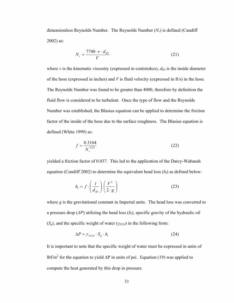
Following the calculations for the individual components, the pressure losses
and heat generation parameters were summed to provide an estimate of the overall
system characteristics that are presented in table 3.4.
Table 3.4: Summarization of the pressure losses and heat generation parameters for each individual component and the estimated system wide parameters.
QuantityPer Unit Total Per Unit Total
Flow Control Valve (FCV) 1 150 150 0.268 0.268Load Check Valve (LCV) 1 5 5 0.009 0.009Directional Control Valve (DCV) 1 2 2 0.004 0.004Quick Disconnect (QD) 8 3 24 0.005 0.043Selector Valve (SV) 1 3 3 0.005 0.00550' of Rubber hose 2 2.85 5.7 0.005 0.01
Hydraulic System 1 189.7 189.7 0.339 0.339
Individual Parameters
System Wide Parameters
Estimated hydraulic loss and heat generationComponent Pressure Loss (psi) Heat Generation (hp)
It is important to note that any pressure losses that may occur due to the flow through
the fittings was ambiguous at this point but not neglectable. From basic fluid
mechanics and empirical data, it is known that head losses in fittings are proportional
to the square of the velocity. Since all the fittings to be used in the hydraulic circuit
were unknown at this point, a factor of safety approach was used. The factor of safety
used was two, therefore doubling the expected pressure loss and the amount of heat
generated by the circuit. This conservative estimate was consistent with the
robustness criteria of being able to repeatedly control the testing without damage to
the machinery.

33
CHAPTER IV
FABRICATION 1. Part Specification
Many of the structural components of the rope testing apparatus were defined
during the final iteration of the design process. The steel used in the fabrication of the
anchor plates, cross head plates, thrust plate, top plate, and left and right c-channels
were specified to be 1018 hot rolled steel. The anchor pins, cylinder pins, and bearing
axels were also specified by the apparatus design calculations to be fabricated of water
hardened tool steel. The bolts securing the anchorages to the c-channel must each
withstand the calculated shearing force of approximately 1200 pounds. Since that
value is approaching the upper limit for a ¼”-20 bolt, a 3/8”-16 steel alloy flat head
cap bolt was specified. The same bolts were also specified to secure the top plate to
the left and right c-channels and to be placed every eight inches on center. It had been
calculated that the radial bearings which guide the crosshead during actuation must be
capable of withstanding a radial force of 1200 pounds and required a ½” bore to
accept the bearing axels. Based on availability and specifications, a ½” plain bore 1”
flat track radial bearing with a load rating of three tons was chosen.
The process of specifying hydraulic parts was a bit more elusive. The
selection of parts depended not only on the hydraulic calculations but also on the

34
requirements imposed by space and mounting requirements. The hydraulic part
specification followed the logic of starting with the linear actuating piston and
working back to the hydraulic power pack, while leaving the lines and hoses to be the
last items that were specified.
In the hydraulic section, it was shown that a hydraulic piston with a two and a
half inch bore and a minimum pressure rating of 1950 psi would be well suited for the
design. Based on the elongation characteristics of standard 3/8” polypropylene and
the minimum specimen length, the stroke length of the hydraulic piston was
determined. A stroke length of 18” was determined to be adequate. The piston was
required to fit between the two c-channels. These two factors led to the design
selection of a 2.5” x 18” 2500 psi rated, double acting, tie rod hydraulic cylinder
manufactured by Prince Hydraulics (Model # SAE-9118).
The extension rate of the piston is controlled with a flow control valve. The
flow control valve also must adhere to the minimum operating pressure rating of 1950
psi. The flow rate for this component is based on that required to extend the piston at
a speed of 144 inches per minute. These requirements led to the flow control valve
being specified as the Prince Hydraulic model number RD-150-8. The RD-150-8 flow
control valve has a maximum pressure rating of 3000 psi and a variable flow rate
between zero and eight GPM.
Addressing a safety concern that was identified during the design phase, a load
check valve was added between the flow control valve and the directional control
valve. This prevents movement of the piston while the directional control valve is in
the neutral position. As with the previous hydraulic parts, the load check valve must

35
withstand a minimum pressure rating of 1950 psi and a maximum flow rate of 19.8
gpm that will be experienced during piston extension or retraction. Prince Hydraulic
model number RD-1450 double pilot operated load check valve met the requirements
with a maximum operating pressure of 3000 psi and a flow rate of 30 gpm.
Control for the direction of actuation was to be accomplished through use of a
directional control valve (DCV). The DCV must be able to withstand a minimum of
1950 psi of hydraulic pressure and a flow rate of 19.8 gpm experienced during
extension or retraction of the piston. Prince Hydraulic DCV part number
RD512CB5A1B1 met these specifications and additionally provided a safety relief
valve set at 2000 psi that would avoid accidental over pressurization of the system.
This particular DCV also allows for power beyond (the ability to add extra DCVs with
minimal plumbing) for future expansion of the apparatus to involve cyclic loading
tests.
The selection between operation of the tow tank wave generator and operation
of the rope testing apparatus is accomplished through a Prince Hydraulic selector
valve (DS-4A4E). This valve has a maximum flow rate of 40 gpm and an operational
pressure range up to 2500 psi. Since this selector valve transfers hydraulic power to
either the tow tank wave generator or the rope testing apparatus, it is critical that it
does not restrict the wave generators’ ability to produce waves of the amplitude and
frequency that are requested by the tank user.
The hoses that connect the rope testing apparatus to the hydraulic power pack
via the selector valve are attached at each end using quick connects. The return line
hose has a maximum working pressure of 2000 psi while the supply line has a

36
maximum working pressure of 3500 psi. These hoses, both of which are ½ inch
diameter, were pre-existing parts from a previous Ocean Engineering initiative. All
steel lines and fittings on the rope testing apparatus were specified to have a maximum
working pressure of 3000 psi. The careful selection of components was deemed
critical to meeting the requirement that the rope testing apparatus be robust and to
ensuring that the operation of the tow tank wave maker, which shares the hydraulic
power pack, would not be negatively impacted.
2. Assembly
Prior to assembly the structural steel components were fabricated. The
engineering drawings that were prepared during the design phase were subject to a
design review process to produce a set of fabrication drawings. The resulting
fabrication drawings, Appendix B, were used to fabricate all the necessary
components. The appropriate machining practices were used during the fabrication of
all parts. Additionally, good assembly techniques were employed which include, but
are not limited to, the application of sealants, lubricants, torque, etc. Assembly of the
structural members and the hydraulic components occurred in parallel as the hydraulic
piston required encasement within the two c-channel sections and top plate.
First, one of the c-channels was attached to the top plate using the 3/8” flat hex
head bolts. The thrust plate bearing material was attached to the thrust plate using the
specified apparatus screws. The thrust plate was slipped into the moving clevis end of
the hydraulic piston and then secured using the manufacture’s clevis pin. This sub

37
assembly was fitted into the pre-assembled c-channel and top plate where it was
secured with the cylinder pin.
Figure 4.1: Assembly drawing showing the placement of piston-thrust plate assembly in the c-
channel-top plate assembly.
The second c-channel was slipped over the cylinder pin and secured to the top plate
and the leg plates were added to each end of the assembly using 3/8” flat hex head
bolts. Finally the stationary anchorage was assembled by bolting the anchor plates to
the two c-channels and slipping the anchor pin through the 1” hole in both plates. This
completed the assembly of all the stationary structural components.
Moving onto the crosshead components, the side bearing plates were attached
to each of the two crosshead plates. The four bearing axels were placed in the
appropriate holes in one of the two crosshead plates. Four of the eight flat track radial
bearings were then slipped onto each of the bearing axels followed by four bearing
spacers. This assembly was slipped onto the rope testing apparatus ensuring that each
of the bearing axels passed through the appropriate holes in the thrust plate. This
stage of assembly is illustrated in figure 4.2.

38
Figure 4.2: Assembly drawing of the crosshead. Note the spacer bearings to isolate the flat radial
track bearings from the thrust plate.
The remaining four bearing spacers were added to the bearing axels followed by the
remaining four flat track radial bearings. The second crosshead plate was slipped over
the bearing axels while taking care to ensure proper alignment. Finally the crosshead
plate was secured. The leg and caster assemblies were constructed and upon their
attachment to the under side of the leg plates, the mechanical assembly of the rope
testing apparatus was completed.
The hydraulic components other than the piston were mounted to the apparatus
in their respective positions. ½” alloy steel tubing was bent to make connections
between components. Hoses, not steel lines, were used to connect the hydraulic
piston. This was intended to alleviate fatigue of the steel lines that may otherwise
have occurred due to motion of the piston. The selector valve was mounted by the
hydraulic power pack as seen in Figure 3.6 and plumbed into the existing tow tank
wave generator circuit according to the manufacture’s recommendations. A male and
female set of quick disconnects sets were connected to two of the ports on the selector

39
valve. Two other male and female sets of quick disconnects were placed on the rope
testing apparatus such that the hoses connecting the power pack and the testing
apparatus could be removed from either or both the power pack and the rope testing
apparatus. The completed assembly of the rope testing apparatus and was followed by
a performance evaluation period for the apparatus. The careful attention to details
during the assembly was part of the intent and design for robustness.
3. Apparatus Testing and Modification
The preliminary testing of the rope apparatus was both qualitative and
quantitative. The purpose of these tests was not to gather data on the rope but to
investigate how the apparatus should be operated to satisfy the robustness criteria of
being operated without extensive training. These tests provided positive insight for
the general operational characteristics of the apparatus and the construction of the
specimens.
The first set of tests involved a qualitative analysis during and after a test
specimen had been loaded to the point of breaking. Items that were considered
included deformation of structural components, check for hydraulic leaks, proper
operation of all valves, relative location of the specimen break, and the extent of
elongation that occurred prior to breaking the specimen.
Although the load cell was in place for the first set of tests, data was not
collected. This was done in order to focus solely on the operation of the apparatus and
construction of the test specimen. The load cell was attached to the anchor pin in the

40
stationary anchorage using a pear link and a clevis which treaded onto the load cell as
shown in figure 4.3.
Figure 4.3: Original method for securing the load cell to the stationary anchorage with clevises
and a pear link. Note that the weight of the securing method is entirely supported by the tension in the specimen.
One end of the rope specimen was attached to the load cell using a second clevis
threaded onto the other end of the load cell, as depicted above. The other end of the
specimen was simply attached to the anchor pin of the moving anchorage via an eye
splice and heavy duty thimble. The two eye splices were constructed in accordance
with the recommended procedures of the CIs’ manual. The splices were each
constructed around a heavy duty thimble, to prevent any flattening of the rope around
the anchor pins, and finished with a series of five tucks. Once the specimen was
secure, the piston was actuated in the extend mode until the specimen broke or the
piston reached the full extent of its stroke.
This test was repeated several times and resulted in the following observations
and speculation about the potential causes. First and foremost, no deformations,
yielding, or failure of any structural components were observed. Likewise, no
hydraulic problems were observed with the exception that the selector valve was

41
observed to have some blow-by into the wave generation circuit which caused a build
up of back pressure on the return line of the wave generation circuit. The relative
location where the specimen broke did, however, raise some concerns. All specimens
broke at the end that was attached the load cell. Even more concerning was the
observation that the brake occurred either in the splice or the eye. It was suspected
that the weight of the load cell, in conjunction with the weight of the clevises and pear
link, were contributing factors adding to the break occurring at the stationary
anchorage end.
The attachment of the load cell to the stationary anchorage was reconfigured
such that the weight of the load cell was supported by the apparatus and not by the
specimen under test. The modification consisted of fastening a steel plate, called the
load cell plate, on the end of the stationary anchorage with the load cell attached at the
same height as the anchor pin. This is depicted in figure 4.4.
Figure 4.4: Modified stationary anchorage to support the entire weight of the load cell and
termination.
Another series of tests were conducted to evaluate the modified anchorage for the load
cell. Although the new tests revealed that the end at which the specimen broke

42
seemed to be random in nature, the break still occurred within the tuck section or the
eye section of the splice. Examination of the specimens at their point of failure
indicated that the majority of the breaks occurred where the “working” end of the rope
re-enters the “running” end of the specimen. This was manifested as a fray in the
throat of the thimble, as seen in figure 4.5.
Figure 4.5: Fray location in relation to the thimble. Notice the fray occurring in the strand
closest to the throat of the thimble.
Closer investigation of the three strands at the throat of the thimble showed that two
strands had broken cleanly in the expected manor. The third strand however, looked
as if it had been crushed. This dissimilarity of breaks became even clearer when the
ends of the three strands underwent a side by side comparison, as shown figure 4.6.
Figure 4.6: Yarn comparison. The two lower yarns exhibit a typical failure mode while the top
yarn seems to have been crushed. The top yarn is the same one showing a fray in figure 4.5.
43
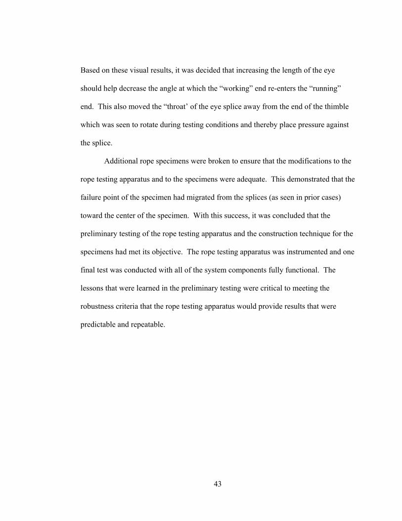
Based on these visual results, it was decided that increasing the length of the eye
should help decrease the angle at which the “working” end re-enters the “running”
end. This also moved the “throat’ of the eye splice away from the end of the thimble
which was seen to rotate during testing conditions and thereby place pressure against
the splice.
Additional rope specimens were broken to ensure that the modifications to the
rope testing apparatus and to the specimens were adequate. This demonstrated that the
failure point of the specimen had migrated from the splices (as seen in prior cases)
toward the center of the specimen. With this success, it was concluded that the
preliminary testing of the rope testing apparatus and the construction technique for the
specimens had met its objective. The rope testing apparatus was instrumented and one
final test was conducted with all of the system components fully functional. The
lessons that were learned in the preliminary testing were critical to meeting the
robustness criteria that the rope testing apparatus would provide results that were
predictable and repeatable.

44
CHAPTER V
INSTRUMENTATION 1. General System Overview
Two primary parameters remained that needed to be characterized. These
included the loading of the specimen and the relative change in length between the
gauge marks on the specimen. These two parameters must be measured throughout
the duration of the experiment. Typically a load cell, in conjunction with an
extensometer, is used to record the load and extension over time. A potential safety
hazard exists with this technique, because the extensometer must be removed prior to
the parting of the rope to prevent instrument damage. The removal of the
extensometer must be done by reaching over the specimen while it is under tension
that is close to the breaking load.
During these experiments a load cell was used in line with the specimen to
acquire the load information. The important deviation from prior practice was
removing the extensometer by using video cameras and imagery tracking software to
extract the changes in distance between the gauge marks.
The measurement system consists of four parts: (1) a load cell with analog
output, (2) an analog to digital (A/D) converter, (3) two digital video cameras, and (4)

45
a laptop running a customized logging program called Synchro. The data flow can be
seen in the block diagram of figure 5.1
Figure 5.1: Block diagram showing the data flow during the experiment and the transfer of video
data via 1394 protocol to the laptop.
The load that was being applied to the specimen under test with the rope
testing apparatus was measured using an industry standard tension/compression load
cell. The load cell, an Omegadyne Inc. (Part number: LC202-2K) had a calibrated
dynamic measuring range between zero and two thousand pounds. The LC202 model
series load cells are constructed of stainless steel and are environmentally sealed.
These two features are advantageous during testing of salt water soaked specimens.
The manufacturer provides each load cell with a NIST certified five-point calibration
at 0(twice), 50(twice), and 100(once) percent of full scale load. This provides
traceability and confidence in measurements that are acquired during tests. The load
cell outputs an analog voltage in the microvolt range. A bridgesensor (Omegadyne
Model number DMD-465WB) was used in conjunction with the load cell. The
bridgesensor provides the excitation voltage required by the load cell and amplifies the
load cell output voltage. This provided the load cell with a stable output voltage that

46
was on the order of millivolts per pound rather than the native output which would
have been on the order of microvolts per pound.
The millivolt per pound output levels allowed the data to be measurable with
an existing A/D converter. The A/D converter is housed in a device known as the
“SLUG”. The SLUG, incorporates a BL2000 Wildcat single board computer. The
BL2000 digitizes the load cell’s output analog signal at 15 Hz into 4096 quantization
levels representing voltages between ±10 volts and outputs a NMEA string containing
the information. This string, along with the Local Application Control Bus System
(LANC) information from each camera is sent via RS232 serial protocol to the laptop
running SYNCHRO software where it is time tagged and recorded.
The elongation data was extracted using digital videography. For simplicity,
image processing that is designed to track linear changes, usually is set to track a
particular feature such as the transition from a black stripe to an adjacent white stripe.
Therefore black and white stripes were placed next to each other on the specimen to
serve as gauge marks. Note that in figure 5.2 it is readily observed that the left gauge
mark is distinguishable from the right gauge mark by the “sense” of the transition.
One being from black to white compared to the other being from white to black.

47
Figure 5.2: Gauge mark placement. The distance between the black white and white black transitions (top) is one foot which is equal to the CI guidelines recommendations. Also in
accordance with CI guidelines the minimum distance from the end of the splice (bottom) is also one foot.
Two Sony Hi8 Digital video cameras (Model number DCR-TVR230) were employed.
Each camera was trained onto one of the two gauge marks and used to record the
movement of that individual set of stripes as a function of time. This method does not
produce immediate elongation data, however through post-processing, this method
produces highly accurate changes in length over the 1-foot gauge length. This method
will be discussed further in the data processing portion of this thesis.
The correlation between the load cell data and the elongation data is provided
by a data logging program developed at the University of New Hampshire’s Center for
Coastal and Ocean Mapping called Synchro. Synchro, developed by Dr. Yuri
Rzhanov is a serial port logging program that continually polls the user specified serial
ports and immediately responds to the arrival of new data. After the serial ports are
sampled the information and corresponding time are then streamed to a user specified
file. Three serial ports were used for acquiring the necessary data during the testing:
(1) load cell data via the SLUG, (2) “right” camera LANC information, and (3) “left”

48
camera LANC information. In addition to the precise logging of the load cell data, the
time synchronization of the LANC information with the load cell data is crucial for
accurate quantitative results. The LANC information contains the frame number,
referenced to the beginning of the digital media, which is recorded synchronously with
the load cell data readings. This allows the elongation data measured via the video
cameras to be matched in time with the load data during post processing. This
provides the ability to develop stereotypical plot of engineering stress-strain which
completely characterizes the rope up to breaking as opposed to just determining the
ultimate breaking strength. Without the ability to make measurements up to the
breaking point, it would not have been possible to make measurements of the strain
hardening region of the engineering properties. That would have obscured one of the
important findings of the experiment (as discussed in 8.3 Engineering properties)
which was the brittle-like property of the WSR near the breaking load.
2. Measurement System Error Analysis
Each element of the measurement system contributes an inherent error that
must be associated with each data point that is reported. The errors propagate through
the various measurements and calculations to generate a level of uncertainty for every
measurement made and every value computed. Starting with the load cell and
continuing through the image analysis, the uncertainty will be calculated for each
component as well as for the entire system based upon manufacturer specifications
and laboratory measurements conducted prior to the experimental runs.

49
The load cell was provided with a certified calibration by the manufacturer.
Beyond this certification, the manufacture specifies that the accuracy of the load cell is
±0.25% of the full scale output. This means for a cell with a maximum load limit of
2000 lbs the measured load will be within plus or minus five pounds of the true value.
This correlates to a voltage uncertainty of ±60.5 µV for the native analog voltage
output of the load cell. Since this was fed into the bridgesensor, any error associated
with amplification of the signal must be included. A laboratory exercise was
conducted to determine the gain factor applied to the bridgesensor’s input signal (see
3. Instrument Calibration). This showed that the bridgesensor was amplifying the
input signal by a factor of 267.8, with a coefficient of determination of 99%. The
error associated with the gain uncertainty equated to ±0.12% of the full scale output
voltage of the bridgesensor.
The Wildcat BL2000 analog to digital converter housed in the SLUG also
impacts the accuracy and precision of the individual load measurements. The Wildcat
BL2000 is a 12 bit A/D converter with a maximum input range of ±10 volts. This
means that the quantization level, or voltage resolution, is 0.005 volts. The error
associated with a recorded A/D voltage is plus/minus one-half of the quantization
level.
The errors associated with measuring the lateral movement of the gauge marks
are affected by several factors. These factors include the distortion due to the
curvature of the lens, the field of view, and the processing technique of extracting the
transition point between the black and white stripes. Lens distortion errors will cause
objects to appear to move more in the center of the frame of view and less along the

50
edges of the frame of view. This distortion can be removed by mathematically
applying a radial correction factor to each of the frames of the video. However, even
this correction has errors associated with it. Based on the worst case scenario seen
during the lens calibration process, the residual errors after the distortion correction
were on the order of ±0.5 pixels.
The second factor affecting the resolution of the lateral movement
measurement is the camera’s field of view. Since the lateral movement of the gauge
marks from right to left is in a single horizontal plane, the conversion between
horizontal distances and image pixels is of primary interest. If both gauge marks were
to be captured by one camera the horizontal field of view at the gauge marks would
have to be up to 30 inches width. Since the camera segments the horizontal field of
view into 720 pixels, the image resolution in that case would at best be ±0.042 inches
per pixel. If two identical cameras are utilized, one for tracking each gauge mark
independently, the horizontal distance resolution of each camera increases to ±0.021
inches per pixel.
Post processing of the video data to extract the transition point between the
black and white stripes of each gauge mark exhibits the greatest uncertainty of the
three factors. This is due in large part to the compounded effect of lens distortion
correction errors and field of view resolution. Additionally, the processing method,
which is described in the data processing section, is only estimating the black-white or
white-black transition between the stripes to the nearest pixel. Together the three
factors lead to a horizontal distance measurement resolution of ±0.022 inches per pixel
per camera. The key here is per camera. Remember in order to achieve elongation

51
data from the two-camera method, the movement of the gauge mark in one camera
must be differenced with the movement of the other gauge mark in the other camera.
This leads to a combined measurement error of ±0.031 inches per pixel.
The last error associated with the experiment is timing or matching of the load
data with the elongation data via the Synchro program. The Synchro program
effectively samples the LANC data available at the communication ports of the
computer at a rate of 15Hz. The LANC information changes at the frame rate of the
cameras which is essentially 30Hz. Therefore the sampling rate of the Synchro
program is the limiting factor in resolving the correspondence between a load cell
measurement and the video frame capture. This does not negatively impact the load
measurement error except for the load at breaking. Since the load is nominally
continually increasing at a fixed rate, the actual load at the breaking point, which
obviously occurs between two of the 15 Hz samples, must be larger than the load that
was measured on the sample just before the sample that detailed the break. This
results in a bias of half the nominal change in load between two measurements and
increases the variance of the measurement by q2/12 where q is the nominal change in
load between measurements. Therefore an additional uncertainty of ±0.024 volts
needs to be summed in quadrature with the error associated with the A/D quantization
level to estimate the uncertainty in the load at the breaks. This combination of the
sampling error and the A/D quantization error produces a calculated uncertainty of the
breaking point of ±0.026 volts. For all other load values the ±0.012 volts uncertainty
is that associated with just the load cell amplification and the A/D conversion. The

52
measurement uncertainties for the physical and engineering properties of the
experiment are easily seen in table 5.1
Table 5.1: Measurement uncertainties associated with all equipment used during experimentation.
Measurement Parameter
Measurement Uncertainty
Unit of Measure
Physical propertiesDiameter 0.001 inchLength 0.016 inchMass 0.002 lbs
Engineering propertiesLength 0.063 inch
Diameter 0.001 inchLoad Cell 0.25% Full Scale volts
Bridge Amplifier 0.12% Full Scale voltsWildcat BL2000 0.005 voltsBreaking point 0.026 volts
Lens Correction 0.5 pixelsPixel Resolution 1 pixels
Calculated measurement uncertainties
3. Instrument Calibrations
Calibration of several instrumentation packages were required to ensure
accurate results and to keep the propagation of error to a minimum. The actuation
(extension) speed of the hydraulic ram was measured several times to ensure that the
rate was indeed 144 inches per a minute and that the speed was consistent time after
time. The bridgesensor’s amplification stage was determined. Finally, the calibration
constants for the video camera lens distortion were computed.
The actuation (extension) speed of the crosshead needed to be calibrated in
order to assure compliance with the Cordage Institute’s guidelines. These guidelines
require the uncycled strength and strain test to be conducted under a constant strain
rate. The speed of the crosshead was calculated based on the time it took the

53
crosshead to travel a specified distance. The time measurements were made with a
pair of PASCO Scientific optical gate timers (Model number ME-9215A) and were
implemented as seen in figure 5.3
Figure 5.3: Setup used to calibrate the crosshead speed. The final setting was assured to be at a
rate of 144 inches per minute.
A series of five trials were run at each setting of the flow control valve. It was
determined that with the flow control valve set to “number four”, the crosshead
traveled at the desired rate. This was re-checked prior to the start of testing. The
results are presented in figure 5.4 with the trial number plotted against the measured
crosshead travel rate.

54
Figure 5.4: Calibration plot of the crosshead travel rate. The final setting was at a level of 145.44
inches per minute.
The flow control valve was set on “number four” to provide a crosshead travel rate at
144 inches per minute for all the experimental runs.
The bridgesensor was calibrated to relate the input voltage to the output
voltage in terms of a gain factor. This is necessary in order that the manufacturer’s
certified calibration can be used during the post processing of the data. The load cell
was connected to the bridgesensor in the manor described by the manufacturer. The
load cell was attached between a mooring weight at one end and an overhead chain
fall at the other. The chain fall was incremented until a portion of the force due to
gravity acting on the weight had been taken up by the chain fall in figure 5.4.

55
Figure 5.5: Bridgesensor calibration setup.
The output voltage from the load cell was measured to ± 0.001 mV with a Fluke
(Model 189) multimeter and compared with a similar measurement made with the
Fluke multimeter at the output terminals of the bridgesensor. This was repeated
several times until the weight was lifted off the floor. The weight was returned to the
floor and the set of input-output voltage measurements were repeated at zero load.
The ratios of the outputs to the inputs were plotted to obtain the gain curve for the
bridgesensor, figure 5.6.
Figure 5.6: Calibration curve for the amplification stage of the bridgesensor.
This curve was combined with the manufacturer’s calibration to produce a curve
associating the load applied to the load cell with the output voltage of the

56
bridgesensor, figure 5.7. A curve fit was then applied to this data to establish an
equation that can be used to convert the A/D voltages back to loads during post
processing.
Figure 5.7: Load cell calibration combined with bridge sensor calibration. This relates final
output voltage to load experienced by the load cell
Prior to recording the video data, a calibration was preformed to determine the
distortion characteristics of the lens on each camera. This step was completed so that
the distortion affects of the lens can be removed during post processing. The video
cameras were set in their final test positions and the zoom made equal in both cameras
and equal to what would be used in the tests. A video image capture was performed
such that a checker board of black and white blocks was oriented in a variety of
angles. A Matlab tool box for camera calibrations, developed in open source code by
the California Institute of Technology and Intel, was implemented. This program
produced correction coefficients for the lens focal length, principal point, lens
distortion, pixel error and the uncertainties for each correction coefficient.

57
CHAPTER VI
ROPE TESTING 1. Experimental Design
The objective of these experiments was to characterize Whale Safe Rope and
show the robustness of the experimental procedure. The characterization process
involved both the definition of the physical properties and the engineering properties
of dry WSR as well as saltwater soaked WSR. This lead to defining the experimental
factors to be: (1) the properties of dry WSR compared to polypropylene and (2) the
effects saltwater soaked WSR cordage. These experimental factors lead to the
development of three treatment combinations.
These treatment combinations are: (1) Dry WSR, (2) Wet WSR, and (3) Dry
Polypropylene. A conscious effort was made to reduce the categorical factors by
purchasing the WSR and the polypropylene rope from the same manufacturer, the
construction of all the specimens by a single person, and keeping the test conditions
constant in all experimental runs. This should provide more accurate and precise
definition of the continuous factors through the physical and engineering properties of
the rope specimens.
Before starting the tests it was necessary to quantify the number of replicate
specimens to use in each of the experimental runs. The characteristics of the

58
specimens in the sample population must adequately represent the characteristics of
the parent population. Since Whale Safe Rope is brand new and not a continually
produced product, the statistical parameters of the parent population are unknown. In
short there is no production history at this juncture. As a start, the nonexistent parent
WSR population was considered to exhibit the characteristics of a well behaved
standard normal distribution. With this assumption, the Central Limit Theorem
applies and the determination of the number of samples (n) need to represent the
parent population (Vining 1998) can be written:
22
⋅≥
Bz
nσα (25)
where zα/2 is the probability standard random variable based on the degrees of
freedom, σ is the population standard deviation, and B is the measure of the width of
the confidence interval. Since the standard deviation of the population is unknown,
the ‘z’ statistic and the standard deviation are replaced by the student’s t-distribution
and the variance to determine a sample size (Schenck 1961). If the student’s t is
plotted against the degrees of freedom with varying confidence levels, as shown in
figure 6.1 a cost benefit analogy can be conducted to determine the number of
replicates required to yield creditable results.

59
Figure 6.1: Graph of the Student's t-distribution with varying confidence levels. Note that as the degrees of freedom goes above 32 it can be shown that the Student's t-distribution approaches the
'z' statistic.
Figure 6.1 reveals that there is not much to be gained by conducting more than 32
replicates per treatment combination. For this study it was decided that 40 replicates
would be conducted to provide a safety buffer in case of machine malfunction, data
collection errors, or ill behaved statistical data distributions.
These parameters defined that this study should conduct three sets of
experimental runs: a dry WSR run, a wet WSR run, and a reference run using standard
polypropylene. All samples must come from the same manufacturer and must be
prepared by the same individual to ensure consistency. The number of samples for
each experimental run was set at 40 for a total of 80 WSR specimens and 40 standard
polypropylene specimens.

60
2. Procedure
There are two important factors in the identification and classification of new
types of cordage material. These are (1) the physical properties and (2) the
engineering properties. The physical properties include the calculation of the
reference tension, initial tension and the measurement of the size number and linear
density of the line. The engineering properties include the uncycled strength and
strain measurements. While the Cordage Institute Guidelines outline many of the
procedures for conducting these tests, the procedures actually used for conducting all
the aforementioned tests will be discussed along with any idiosyncrasies associated
with the setup in this study.
The first set of tests to be completed involved the determination of the physical
properties of the Whale Safe Rope. Before any tests could be completed the reference
tension, a low tension that does not change the properties of the specimen, needed to
be calculated. The Cordage Institute defines the reference tension (RTp) as:
250 dRTp ⋅= (26)
where d is the nominal diameter of the specimen. If the nominal diameter is not
known a measure can be conducted under light hand tension. The UNH method
used a nominal diameter of 3/8 of an inch as a first iteration. In accordance with the
CI guidelines, a section of WSR rope was secured to an overhead beam and a weight,
dictated by the calculated reference tension, tied to the opposite end to provide the
necessary tension, as seen in figure 6.2.

61
Figure 6.2: Setup for determining the Physical properties (nominal rope diameter, rope number,
and linear density).
Measurements of the diameter were acquired with the use of a machinist vernier
calipers ensuring that at least two strand crowns were in contact with each side of the
caliper jaws at all times. The measurements were repeated at a spacing of typically
three inches but no less then least two inches. At this point according to CI guidelines
if the average measured nominal diameter varied more than 10%, the process must be
iterated. The iteration must start with the recalculation of the reference tension using
the average nominal diameter value.
Once the nominal diameter met the criterion of less then 10% variation, the
size number was calculated by multiplying the measured nominal diameter by Pi.
Additionally, the initial tension (ITp), in units of pounds was calculated by:
2200 dIT p ⋅= (27)
The amount of weight at the end of the specimen was then adjusted to meet the initial
tension criterion. One gauge mark was then placed one inch from the top termination

62
and a second placed ten inches below the first to an accuracy of ± 1/16 of an inch.
Since the length of the specimen under tension was greater then the one foot
requirement by the CI guidelines for this test, a series of ten inch increments were
marked out with a minimum of one inch separation between them. A utility knife was
used to cut on theses marks to produce a ten inch specimen for the measurement of
linear density. This is repeated until the proper number of linear density specimens
are produced. The linear density specimens were then weighed to an accuracy of ±1%
with a Mettler 1200 electronic balance. With the precise weight (P) in pounds and
length (F) in feet known, the linear density per 100 feet (LDp) of WSR is calculated
by:
⋅=FPLDp 100 (28)
The ends of the specimens were then taped to prevent any fiber loss or unwrapping.
Additionally, the specimens were numbered, bagged, and inventoried until all
processing was complete. This ensured that any question that may arise during post
processing might be resolved by reviewing any particular specimen.
The next portions of the experimental test were aimed at defining the
engineering properties of the WSR. This began with preparation of the samples that
would be tested as dry WSR, wet WSR, and standard polypropylene. As mentioned in
the experimental design section, 40 specimens were prepared for each of these tests.
Each specimen length was marked on the axis to which it was unraveled from the
spool and cut to a length of approximately 90 inches. The cut specimen was then
transferred to a jig in order to set the length of the eye splices and to ensure that no
twists were introduced. The length of each eye splice was controlled to be 6.5” in

63
length and was constructed with five tucks securing the splice. The final length of the
test specimens, center to center between eye splices, was 62 inches
Each of the newly spliced specimens was placed under the specified initial
tension. Two marks were placed on the specimen with a permanent black marker.
One mark was 12 inches from the end of the splice that was to be secured onto the
stationary anchorage and another one was 12 inches from the first mark. These two
marks indicated where the black to white, or white to black transition would occur
between the stripes. Tape was applied to mask the rope during the painting of the
black stripes, which extended one inch along the rope as seen in figure 6.3.
Figure 6.3: Depiction of masking for the painting of the black stripes.
It is important to note that in the above figure that the black stripes occur on the
outside of the black marker marks placed on the specimen. After the black stripes had
thoroughly dried, tape was applied one inch inside the black marker marks to mask the
rope for the painting of the white stripes. A clear tube was slid over the black painted
stripes to protect them from over spray during the painting process. This is illustrated
in figure 6.4.

64
Figure 6.4: Depiction of methodology used to paint white stripes. Notice the clear plastic tubes
over the black stripes (outside).
A latex based paint was used so that the addition of the paint to the rope would have
minimal affects, if any to the properties of the rope.
The specimens for the dry WSR and the standard polypropylene were ready to
undergo testing at this point. However, the samples slated for use in the wet WSR
tests required soaking in a bath of saltwater. This was accomplished by combining
twenty gallons of cold tap water with 2365.8 mL of an artificial sea salt concentrate.
Using a Fisher Scientific hydrometer (model 11-529-A), a Neslab Instruments
thermometer, and an Odem Hydrographic digibar pro sound velocimeter (model
DB1200), the salinity was estimated as 31.49 PSU. The specimens that were slated
for wet testing were draped into the saltwater solution ensuring that the eye splices
were kept out of the water, as seen in figure 6.5
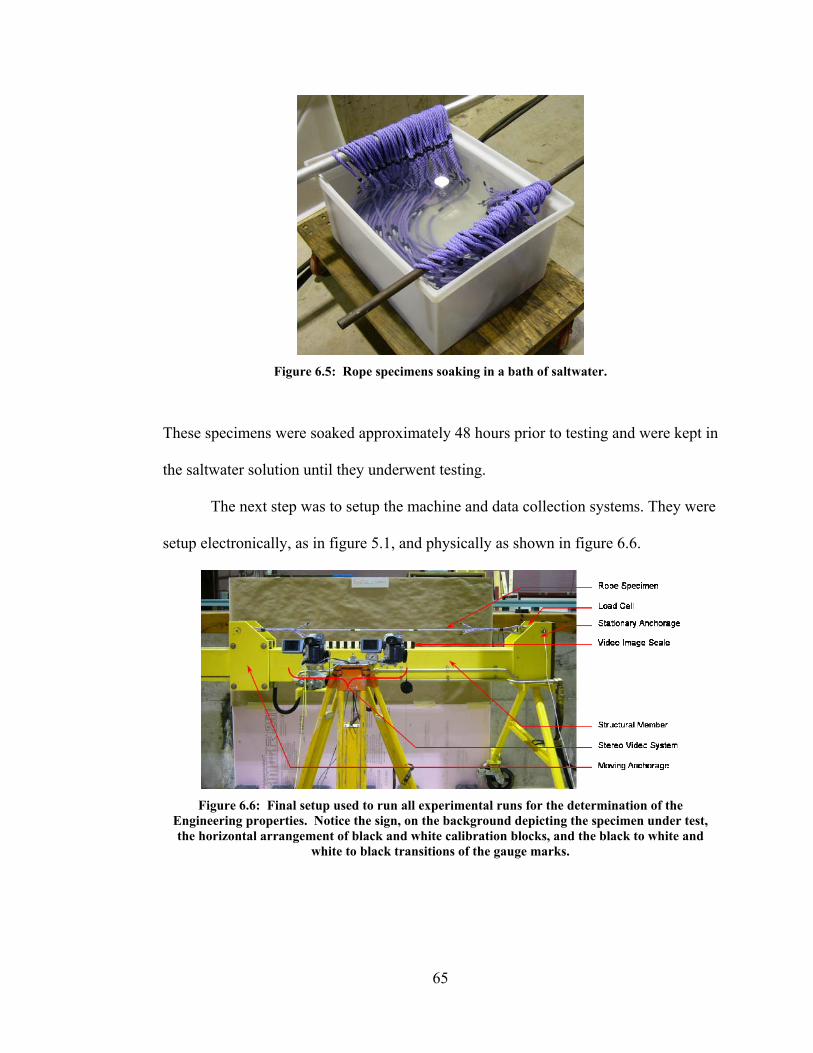
65
Figure 6.5: Rope specimens soaking in a bath of saltwater.
These specimens were soaked approximately 48 hours prior to testing and were kept in
the saltwater solution until they underwent testing.
The next step was to setup the machine and data collection systems. They were
setup electronically, as in figure 5.1, and physically as shown in figure 6.6.
Figure 6.6: Final setup used to run all experimental runs for the determination of the
Engineering properties. Notice the sign, on the background depicting the specimen under test, the horizontal arrangement of black and white calibration blocks, and the black to white and
white to black transitions of the gauge marks.

66
It is important to note that the video image scale with its horizontal alternating blocks
of black and white is directly under the center line of the specimen and the right hand
edge is vertically aligned with the right hand white black transition point. The
distance between the camera lenses and the video image scale was set to 32 inches and
the height of the camera lenses were aligned on the center line of the rope specimen.
The separation distance between centers of the camera lenses was one foot, the same
as the distance between the gauge marks on the specimen. The two cameras were
turned on and the zoom on each was adjusted to ensure that the field of view would be
equal on both video recorders. Also at this point, the tripod is moved right to left such
that gauge marks are guaranteed to be located in the right hand side of the individual
cameras field of view.
A background was placed behind the test machine to reduce the possibility of
vertical lines of contrast in the video. This was done to reduce contrast changes in the
background which improved the tracking of the white-black and black-white
transitions. This also allowed a small sign to be placed on the background indicating
which sample specimen was under test.
Once the setup was completed, a series of system checks were preformed. A
video calibration was conducted for each camera as outlined in chapter five. Prior to
mounting the specimen, the load cell zero point was checked for any DC offset and
adjusted if necessary. The logging software was tested for proper port and channel
trigger settings. A dry run of the experiment was preformed where an extra rope
specimen was placed in the testing machine. The acquired data was checked for
validity before moving on to the actual experimental testing stage.

67
All the rope specimens that were tested and used to determine the
characteristics of the WSR and the reference industry standard polypropylene were
tracked. Each specimen was given a unique serial number. For example, the serial
number S000D was assigned to a dry WSR specimen number zero that was used in the
dry run test. These serial numbers are affixed to plastic storage bags that contain the
specimen before and after the test run. In addition, the serial number was used for the
basis of associating collected video and data files to a particular specimen. During the
experiment a log sheet was used to track various items. These items include the
starting frame numbers of the left and right cameras, data file names, date, time,
position of break, qualitative break data, and other pertinent information about each of
the experimental runs.
Finally, the experiment was ready to commence. In this particular study, the
dry WSR tests were conducted first, followed by the saltwater soaked WSR tests and
finally the reference polypropylene. The specimen under test was mounted in the
grips of the machine with one gauge mark located 12 inches from the eye splice on the
stationary anchorage end. The experimental protocol required that the mark which
indicated how the rope was taken off the coil, was facing up on both ends and that no
twists were added to the specimen. Once set in the anchorages the specimen’s
termination points were restrained from rotating around the axis of the rope. Since the
gauge marks were applied to the specimens while the samples were under initial
tension, the application of the initial tension, which is part of the procedure outlined
by the Cordage Institute was passed. The Synchro program was reset from standby to
recording mode as were the left and right digital video cameras. The directional

68
control valve was set to put the crosshead into the extension motion. The crosshead
was kept in motion, with all personal at a safe distance, until the specimen parted. The
direction of crosshead motion was reversed and ran until the hydraulic piston was fully
retracted. The specimen was removed from the grips, bagged, and cataloged. The log
sheet for the specimen test was filled out and placed in the serialized bag with the
specimen.

69
CHAPTER VII
DATA PROCESSING 1. General
The data on the physical properties of the WSR and the reference
polypropylene rope were examined. The mean and standard deviation of the nominal
diameter was computed, followed by the size number classification as outlined in the
procedure section. The reference and initial tensions were calculated based on the
measured diameter in accordance with the CI guidelines. Finally the mean and
standard deviation of the linear density was determined in accordance with the CI
guidelines.
The raw data for determining the engineering properties was collected in two
forms. A text file was collected by a laptop containing the LANC information for the
right and left digital video cameras which was matched in time with the data obtained
from the load cell. The two cameras recorded the relative movement of the gauge
marks over time. The digital image data was downloaded to a computer for post
processing. In the post processing stage, the video imagery was corrected for the lens
distortion then a specialized image processing program was used to extract frame by
frame the change in pixels of the white-black or black-white transition of the gauge
mark. The displacements, measured in each of the two cameras along with the

70
corresponding video frame information, were saved to a text file. The load cell text
file and the imagery text file were time aligned and the engineering stress-strain
information was extracted.
2. Video Data Processing
The lens calibration constants were obtained from the lens calibration software
as outlined in the calibration section. The individual replicate runs’ left and right
video captures were downloaded using WinDV and corrected for lens distortion using
the lens calibration constants. The hour, minute, second, and frame number for each
replicate and each camera at which the video captures were started were recorded to
preserve the time link between the load cell data and the elongation (video) data. This
information was collected on the same log sheet that had been used during the
experiments for each replicate specimen and later entered into an MS Excel
spreadsheet for use in the automated Matlab data processing.
The Lens Correct program requires its input be uncompressed video files while
the output of WinDV’s compression format is based on Digital Video (DV)
compression. Therefore the downloaded video captures needed to be resaved in an
uncompressed format. The Lens Correct program could then be used to remove any
distortions in the video capture created by the inaccuracies in the curvature of the
camera lens. The Lens Correct program, whose GUI is shown in figure 7.1 has two
inputs, (1) the uncompressed video in *.avi format and (2) the calibration constants in
a *.txt format.

71
Figure 7.1: Front Panel of the Lens Correct program. The lower window appears when the View
Parameters button is clicked.
The program outputs an uncompressed *.avi file to which the camera lens correction
constants have been applied.
Having systematically removed distortion due to inaccuracies in the curvature
of the camera lens, the captured video frames were ready to be processed for
extracting the horizontal movement of the black-white gauge mark transition point. A
DOS application, called RopeMovie written by Dr. Yuri Rzhanov was used to extract
the pixel location of the black to white and white to black transition points in a single
frame of the video capture file. The program basically moves from pixel to pixel
looking at the change in contrast between horizontal neighboring pixels. The location
where the contrast slope is the greatest is defined as the transition point between the
different colored stripes on the rope. The program then advances to the next frame
and repeats this process, recording the pixel location of the transition with the frame

72
number. The program also characterizes the robustness of the determination of the
transition point. In addition to the input and output file names, several input
parameters listed in table 7.1 were optional that could be specified to increase the
accuracy, precision and speed of tracking the transition point.
Table 7.1: Input arguments for the Ropemovie program which extracts the transition point of the gauge marks as a function of time. The pixel position is recorded in a text file along with the
associated frame number.
Input arguments for RopeMovie program Argument Input Limits Default Values Description
-bw 0 or 1 0 Order of transition sequence (black white or white black)
-d 0 or 1 0 Debugging level (zero is off)
-r 0 to infinity 0 to infinity
0 10000
Range of frames to be processed (starting and ending frame number)
-R 0 to 480 -1 Height of video image scale in pixels (Feature is off when -1)
-s 0 to 720 0 to 480
10 11
Width and Height of either the white or black stripe in pixels
-x 0 to 720 0 to 720
200 500
Range (pixels) in the horizontal where the transition is located
-y 0 to 480 0 to 480
100 400
Range (pixels) in the vertical where the transition is located
in.avi N/A N/A Input file name in avi format out.txt N/A N/A Output file name in txt format
Importantly, the program measures the pixel width of the alternating white and black
blocks on the video image scale (seen in figure 6.6) to provide a link between pixel
space and actual measurable distance. This scaling value is determined for every
frame in the video capture and is included in the output text file.
The Ropemovie program was run for every replicate in the three treatment
combinations for both cameras. This yielded two text files for each replicate, left and
right for a total of 240 text files. The left and right image processing text files were
matched in Matlab with the associated load cell text file for each individual replicate.

73
3. Matlab Data Processing
Once all the video captures had been processed down to their respective text
files, they along with the corresponding load cell data file and the frame reference
Excel file were processed in Matlab. The objective of the Matlab processing was to
produce an engineering stress-strain plot of the data along with an appropriate curve fit
that would accurately represent each of the treatment combinations.
The first step was to align the displacement text files from the video images
with the load cell data in time. Since the LANC information was preserved thought
out the video analysis and it was also recorded with the load cell data, a logical way to
align the three files, (right camera displacement, left camera displacement, and load
cell data) was to match up the hour, minute, second, and frame numbers within each
file. The data was then filtered and only the data points containing the left
displacement, right displacement, and load cell data were kept.
The aligned data needed to be accurately and precisely converted from output
load cell voltages and pixel displacements into actual loads in pounds and
displacements in inches, respectively. The load cell data was converted from volts
into pounds using the calibration curves that were obtained during the load cell
calibration process. The conversion from pixels to distance in inches was a bit more
involved. The change in specimen length between the two gauge marks from one
frame to the next was initially computed in the pixel domain. Delta length in pixels
was converted to inches by taking the mean of the number of pixels in each of the
alternating black and white blocks contained in the ruler column of the Ropemovie
text file for each camera. The right camera length measurements, which was tracking
74
the gauge mark closest to the stationary anchorage of the machine was subtracted from
the left camera length measurements. This yielded the delta length across the entire
gauge length of the specimen, or specifically the elongation. The engineering stress
and strain were calculated by dividing the load and the delta length by the cross
sectional area of the rope at initial tension and the original one foot gauge length,
respectively. This process was repeated for each replicate in each of the three
treatment conditions.
The engineering stress-strain raw data was curve fitted to determine the
mechanical settling, linear elastic, and strain hardening regions. This was achieved
through a piecewise fitting routine. The first and second derivatives of stress with
respect to time were computed to determine concavity and their associated inflection
points. The first derivative revealed a parabolic shape with some data spikes present
that could obviously be considered as outliers. These spikes were detected and
removed from the first derivative of stress. A centered five point boxcar filter was
implemented to smooth the data. The second derivative was computed on the
smoothed data. This revealed a relatively flat data set with a slight negative slope. A
first-round estimate of the mean and standard deviation around the zero crossing of the
filtered second derivative was computed and used to determine limits for the section of
data that could be considered to have a constant slope. The starting and ending indices
of this section of data were acquired and used as the data limits in determining a linear
fit to the engineering stress-strain raw data. The data prior to the starting index and
following the ending index were each fitted with a second order polynomial fit. This
process was repeated for all replicates in the three treatment conditions.

75
All of the curves and their associated statistics in a particular treatment
condition were combined into a single curve that represents the forty replicates in the
treatment condition group. Finally the two WSR curves dry and wet, were plotted on
the same graph for comparison purposes.
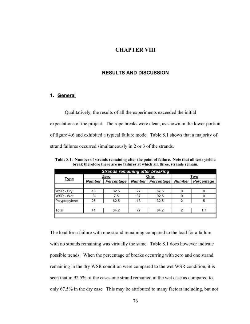
76
CHAPTER VIII
RESULTS AND DISCUSSION 1. General
Qualitatively, the results of all the experiments exceeded the initial
expectations of the project. The rope breaks were clean, as shown in the lower portion
of figure 4.6 and exhibited a typical failure mode. Table 8.1 shows that a majority of
strand failures occurred simultaneously in 2 or 3 of the strands.
Table 8.1: Number of strands remaining after the point of failure. Note that all tests yield a break therefore there are no failures at which all, three, strands remain.
Number Percentage Number Percentage Number Percentage
WSR - Dry 13 32.5 27 67.5 0 0WSR - Wet 3 7.5 37 92.5 0 0Polypropylene 25 62.5 13 32.5 2 5
Total 41 34.2 77 64.2 2 1.7
Strands remaining after breakingType Zero One Two
The load for a failure with one strand remaining compared to the load for a failure
with no strands remaining was virtually the same. Table 8.1 does however indicate
possible trends. When the percentage of breaks occurring with zero and one strand
remaining in the dry WSR condition were compared to the wet WSR condition, it is
seen that in 92.5% of the cases one strand remained in the wet case as compared to
only 67.5% in the dry case. This may be attributed to many factors including, but not

77
limited to, the rate of heat dissipation during the loading of the specimens. The WSR
cases were compared to standard polypropylene and it was seen that the polypropylene
was more apt to have a failure of all three strands. A possible explanation of the
tendency for instantaneous failure of all strands of the polypropylene was the higher
tensile load at failure. As the failure propagates the transfer of load from one strand
to the next occurs at a faster rate than the rate of elongation. Therefore the machine
does not have to “play catch up” to break all three strands.
Further stratification of the specimen failures brings up the question of the
locations of the breaks. None of the 120 specimens tested broke in the terminations.
However, the relative location of the break that occurred within the center section did
vary. These variations are outlined in table 8.2.
Table 8.2: Table showing the varying location of the breaks between the splices. Note that none of the 120 specimens broke in the terminations.
Number Percentage Number Percentage
WSR - Dry 16 40 24 60WSR - Wet 21 52.5 19 47.5Polypropylene 21 52.5 19 47.5
Total 58 48.3 62 51.7
Location of breaks within the center sectionType Closer to Moving Anchorage Closer to Stationary Anchorage
The location of the breaks in all the experimental runs seemed to be fairly evenly
distributed between breaking closer towards the moving anchorage and closer towards
the stationary anchorage. This implied that the experimental process, the rope
machine, and in particular the terminations did not effect the location of the break.
The failure points did not seem to be predetermined by external factors beyond the
specific specimen under test.

78
2. Physical Properties
The physical properties for the Whale Safe Rope were measured. The physical
properties of the Polypropylene were those published by the manufacture. Table 8.3
presents the physical properties of the two types of rope.
Table 8.3: Results of the physical properties tests showing the mean value, standard deviation of the mean, the associated measurement uncertainty with a single measurement, and the percent
error between the standard deviation and the mean. Note that the Polypropylene data is from the manufacturer.
Whale Safe Rope Polypropylene
Mean 1.13 1.18Standard Deviation 0.010 N/AMeasurement Uncertainty 0.003 N/ACoefficient of Variation 0.8 N/A
Mean 3.39 2.8Standard Deviation 0.243 N/AMeasurement Uncertainty 0.020 N/ACoefficient of Variation 7.1 N/A
Linear Density (lbs / 100ft)
Physical propertiesExperimental Test Treatment Combinations
Size Number
The size number of the WSR is approximately 4.2% smaller than that of the
Polypropylene even though both ropes were considered to be in the 3/8” diameter
class. This was in part due to WSR having a much tighter weave as compared to the
polypropylene. The difference in the linear density between the two ropes was due to
the addition of barium sulfate to reduce the breaking strength of the polypropylene
based WSR.
The robustness of the experimental procedure can be examined through
analysis of the standard deviation and the measurement uncertainty. The measurement

79
uncertainty showed the effective resolution of each of the individual measurement that
made up the mean value of a parameter, where as the standard deviation is a measure
of how an individual measurement differs from the expected mean calculated from the
sample set. Table 8.3 shows that all the observed standard deviations were greater
than the calculated measurement uncertainties. This indicates that the instrumentation
used to obtain the parameters for determining the rope properties was not the limiting
factors.
The data closely resembles a well behaved standard normal distribution,
therefore the standard deviation and the ‘z’ statistic was used to determine the number
of measurements in future experiments (as seen in equation (25)) with this procedure
and instrumentation that are required to bound the expected mean within a desired
confidence limit, called the expected mean estimate error. Table 8.4 shows the
expected mean estimate error with various sample sizes for two confidence limits.
Table 8.4: Table of expected mean estimate error used to determine future sample sizes using the present data set as an accurate representation of the parent population.
90% 95% 90% 95%
2 0.012 0.014 0.284 0.3374 0.008 0.010 0.200 0.2388 0.006 0.007 0.142 0.16816 0.004 0.005 0.100 0.11932 0.003 0.003 0.071 0.08464 0.002 0.002 0.050 0.060
Physical expected mean estimate errorNumber of
Rope Samples
Rope Number Linear DensityConfidence Level Confidence Level
The table 8.4 shows that in future experiments a relatively small sample set is required
to reliably estimate the expected mean of each of the physical parameter.
80
3. Engineering Properties
The ultimate breaking strength was extracted from the uncycled strength and
elongation data. As seen in table 8.5, Seaside Inc., who manufactures the WSR,
suggested that the ultimate breaking load of WSR is in the region of 1050 lbs. When
this is compared to the acquired mean seen in table 8.5, along with the associated
standard deviation, it fell within the two standard deviation limit of the UNH data.
Seaside Inc. did not provide an estimate for wet breaking strength of the WSR.
However, there was a marketed difference between the WSR dry and wet breaking
strengths. This difference was attributed to the dissipation of heat by the salt water
contained in the wet combination. The mean ultimate breaking strength for the
polypropylene reflected the published values which range from 2440 to 2900 pounds.
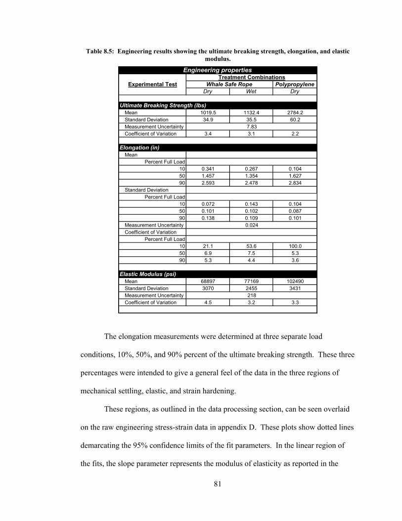
81
Table 8.5: Engineering results showing the ultimate breaking strength, elongation, and elastic modulus.
PolypropyleneDry Wet Dry
1019.5 1132.4 2784.234.9 35.5 60.2
3.4 3.1 2.2
Percent Full Load10 0.341 0.267 0.10450 1.457 1.354 1.62790 2.593 2.478 2.834
Percent Full Load10 0.072 0.143 0.10450 0.101 0.102 0.08790 0.138 0.109 0.101
Percent Full Load10 21.1 53.6 100.050 6.9 7.5 5.390 5.3 4.4 3.6
68897 77169 1024903070 2455 3431
4.5 3.2 3.3
Engineering properties
Experimental TestTreatment Combinations
Whale Safe Rope
Ultimate Breaking Strength (lbs)MeanStandard DeviationMeasurement Uncertainty 7.83Coefficient of Variation
Elongation (in)Mean
Standard Deviation
218
Measurement Uncertainty 0.024Coefficient of Variation
Elastic Modulus (psi)
Coefficient of Variation
MeanStandard DeviationMeasurement Uncertainty
The elongation measurements were determined at three separate load
conditions, 10%, 50%, and 90% percent of the ultimate breaking strength. These three
percentages were intended to give a general feel of the data in the three regions of
mechanical settling, elastic, and strain hardening.
These regions, as outlined in the data processing section, can be seen overlaid
on the raw engineering stress-strain data in appendix D. These plots show dotted lines
demarcating the 95% confidence limits of the fit parameters. In the linear region of
the fits, the slope parameter represents the modulus of elasticity as reported in the

82
lower portion of table 8.5. No published comparison values exist for the WSR.
However, the measured polypropylene’s elastic modulus is about half of the values
reported by the plastics industry. It is theorized that this reduction of elastic modulus
is due to having constrained the specimen to prevent rotation during the test and due to
the multiple strand construction of the WSR. The non-rotational constraint adds a
torque force (based on the helical angle of the weave) to what would otherwise be a
pure tensile force. The test is a valid representation of the condition in which the rope
is deployed in fixed fishing gear without mechanical swivels.
The comparison of the different treatment combinations shows some
interesting results. The first comparison was preformed on the engineering stress-
strain curves between the wet and dry cases of the WSR as seen in figure 8.1.
Figure 8.1: Comparison plot of the curve fits for the WSR dry and wet cases. The green color
represents mechanical settling, the cyan color is the strain hardening region, and the linear sections (red and blue) are the elastic regions.
It can be concluded from figure 8.1 and the values for the elastic modulus in table 8.5
that the salt water soak had a measurable effect on the performance of the whale safe
rope. The dry cases for the WSR and the polypropylene were compared in figure 8.2.

83
Figure 8.2: Comparison plot of the curve fits for the whale safe rope (dry) and polypropylene
(dry).
The ultimate breaking strength and the elastic modulus were obviously very different
between the WSR and the polypropylene. Furthermore, the strain hardening regions
of the two exhibited distinctively different slope characteristics. Appendix E presents
the first derivative of stress verses the linear index number for the various treatment
conditions and comparisons. It is clearly seen that slope of the strain hardening region
for the WSR is much flatter than that of the polypropylene. It is suggested that this
indicates an increase in the brittle properties of WSR compared to the polypropylene.
The second derivative of stress was also computed. The second derivative of
stress plotted against the linear index exhibited a flat region with a slight negative
slope (Appendix F). This is suggestive of “necking” or reduction of the cross-
sectional area of the specimens during the experimental runs. The extraction of the
increase in the brittle properties of WSR as compared to standard polypropylene and
the measurement of the reduction of the cross-sectional area over time from the data is
a unique quality of the implemented data acquisition systems and techniques. The
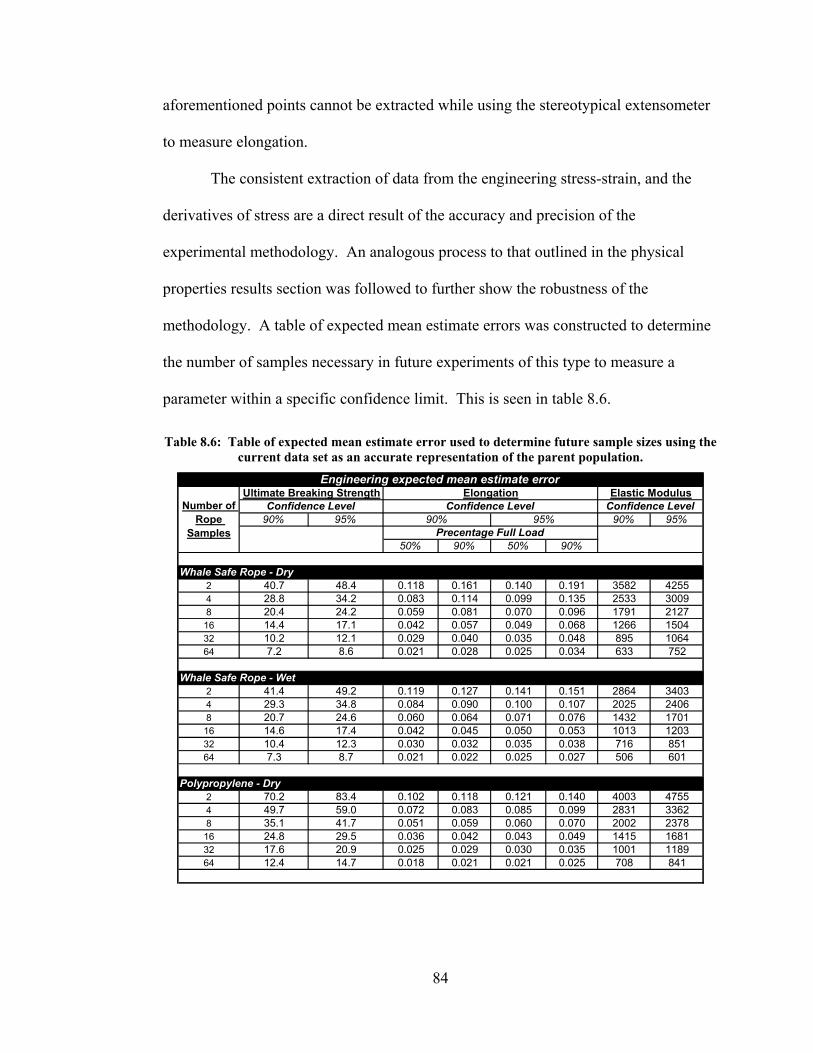
84
aforementioned points cannot be extracted while using the stereotypical extensometer
to measure elongation.
The consistent extraction of data from the engineering stress-strain, and the
derivatives of stress are a direct result of the accuracy and precision of the
experimental methodology. An analogous process to that outlined in the physical
properties results section was followed to further show the robustness of the
methodology. A table of expected mean estimate errors was constructed to determine
the number of samples necessary in future experiments of this type to measure a
parameter within a specific confidence limit. This is seen in table 8.6.
Table 8.6: Table of expected mean estimate error used to determine future sample sizes using the current data set as an accurate representation of the parent population.
90% 95% 90% 95%
50% 90% 50% 90%
2 40.7 48.4 0.118 0.161 0.140 0.191 3582 42554 28.8 34.2 0.083 0.114 0.099 0.135 2533 30098 20.4 24.2 0.059 0.081 0.070 0.096 1791 212716 14.4 17.1 0.042 0.057 0.049 0.068 1266 150432 10.2 12.1 0.029 0.040 0.035 0.048 895 106464 7.2 8.6 0.021 0.028 0.025 0.034 633 752
2 41.4 49.2 0.119 0.127 0.141 0.151 2864 34034 29.3 34.8 0.084 0.090 0.100 0.107 2025 24068 20.7 24.6 0.060 0.064 0.071 0.076 1432 170116 14.6 17.4 0.042 0.045 0.050 0.053 1013 120332 10.4 12.3 0.030 0.032 0.035 0.038 716 85164 7.3 8.7 0.021 0.022 0.025 0.027 506 601
2 70.2 83.4 0.102 0.118 0.121 0.140 4003 47554 49.7 59.0 0.072 0.083 0.085 0.099 2831 33628 35.1 41.7 0.051 0.059 0.060 0.070 2002 237816 24.8 29.5 0.036 0.042 0.043 0.049 1415 168132 17.6 20.9 0.025 0.029 0.030 0.035 1001 118964 12.4 14.7 0.018 0.021 0.021 0.025 708 841
Precentage Full Load
Whale Safe Rope - Dry
Whale Safe Rope - Wet
Polypropylene - Dry
Engineering expected mean estimate error
Number of Rope
Samples
Ultimate Breaking Strength Elongation Elastic ModulusConfidence Level Confidence Level Confidence Level
90% 95%

85
Table 8.6 shows that only a small number of samples are required to achieve the
expected mean of a parameter within limits based on the selected confidence limit.
The claim of a robust process, with the exception of the elongation at the 10% full
load case, is further supported by the reported coefficient of variation experienced in
table 8.5. The elongation within the mechanical settling region is excluded due to the
high variability of the settling of the newly formed splices and transient vibrations of
the machine when first actuated from rest.

86
CHAPTER IX
CONCULUSIONS This study successfully investigated the properties of Whale Safe Rope (WSR)
in an effort to establish a robust experimental methodology for the accurate and
precise testing of rope. The process started with the research, design and construction
of a rope tension testing apparatus and data measurement systems that would yield
accurate and consistent results. The robust experimental methodology that was
devised for testing the rope to ultimate failure achieved high accuracy of the
elongation measurement through the implementation of digital image processing
making it easy for an operator to safely achieve high repeatability without having
extensive specialized training.
The physical and engineering properties of WSR presented in tables 8.3 and
8.5, respectively, show various parameters that are required in order to make informed
decisions about the design and implementation of offshore gill net and lobstering
rigging. It is noteworthy that WSR shows evidence of properties that are analogous to
those of a material with brittle characteristics. This means that the WSR might very
well break at the location of a point (whale) load. The aforementioned charts and
figures show a high degree of precision which allows insight into the mechanics of the
specimen under test.

87
Statistical analysis of the experimental data, as presented in tables 8.1, 8.2, 8.4,
and 8.6, show both qualitatively and quantitatively the robustness of the experimental
methodology. These tables show that future experiments can achieve significant
results by testing only four replicates per treatment combination and still guarantee
that 95% of the data will contain the expected value of a particular parameter to within
the same standard deviations as noted in the physical and engineering properties
tables. This outstanding result stems directly from the methods that were devised and
then used to gather and process the data.
The data in tables 8.1 and 8.2 further demonstrates that the bed length chosen
for the testing machine was reasonable. This directly reflects the fact that the design
process correctly weighed the design criterion to minimize the fabrication cost and
maximize the data quality and repeatability.
There are, however, a few points worth addressing for future testing. The
errors of the measurements deemed to be in the mechanical settling region of the
engineering stress-strain curves were higher than those exhibited elsewhere. The high
standard deviation is largely attributed to the video cameras having been mounted to a
tripod that was independent and remote from the frame of the rope testing apparatus.
Affixing the cameras directly to the frame of the testing apparatus will likely reduce
these errors and possibly provide greater insight into the mechanical settling
characteristics of the terminations.
The method of attaching the specimens to the machine may possibly be
redesigned to eliminate the need to construct an eye splice at each end of the
specimen. This would allow for quicker testing and the nondestructive testing of field

88
deployed line, which typically is hard to splice. It is also arguable that this method of
attachment, if done carefully, will settle no more than that of an eye splice. However,
care must be taken to assure that if any extended settling of the rope on the termination
does occur, it can be neglected in favor of the other benefits that this type rope
attachment would bring to the operation. This modification to the test apparatus could
be beneficial for gaining insight into the performance characteristics of WSR, or any
line, over time. The addition of a cyclic loading test should also be considered to give
a further basis for comparisons between different types of ropes. This possibility of
including cyclic load testing was foreseen in the design stage of the testing apparatus
and consequently provisions were made that would make it relatively easy to
exchange the present direction control valve for a computer controlled solenoid
control valve. These additional modifications and experimental tests will allow future
researchers and end-users of any rope/line to better understand the most common
piece of equipment which impacts cost and safety in the marine industry. That is to
say, rope.

89
REFERENCES ASTM. (1993). Standard Methods of Testing Fiber Ropes. Annual Book of American Society for Testing and Materials Standards, Vol. 7, D4268 – 93, 397 – 403 p. Beer, F.P., and Johnston, E.R. (1996). Vector Mechanics for Engineers: Statics. McGraw-Hill, Inc., New York. 599 p. Caswell, H., Fujiwara, M., and Brault, S., (1999). Declining survival probability threatens the North Atlantic right whale. Proceedings of the National Academy of Sciences. 3308 – 3313 p. Cavatorta, D., Starczak, V., Prada, K., and Moore, M. (2003). Friction of Different Ropes in Right Whale Baleen: a Potential Strategy to Reduce Entanglement Mortality. North Atlantic Right Whale Consortium Annual Meeting, Feb 4&5. CI. (1999). CI 1301-96: Polypropylene Fiber Rope. Cordage Institute Standards, Ver. 2, Wayne, PA. CI. (2002). CI 1500-02: Test Methods for Fiber Rope. Cordage Institute Standards, Ver. Feb 2002, Wayne, PA. Cundiff, J.S. (2002). Fluid Power Circuits and Controls. CRC Press LLC, Florida. 533 p. Flory, J.F., and Mercer, D.E. (1997). The New Cordage Institute Fiber Rope Test Methods. Oceans ’97 MTS/IEEE Conference Proceedings, Vol. 1, 308 – 313 p. Frady, T. (2004). Guide to: The Atlantic Large Whale Take Reduction Plan. NOAA/NMFS/NER, http://www.nero.noaa.gov/whaletrp/. Frocht, M.M., and Hill, H.N. (1940). Stress-Concentration Factors Around a Central Circular Hole in a Plate Loaded Through Pin in the Hole. Journal of Applied Mechanics (Transactions of the American Society of Mechanical Engineers), Vol. 7, No. 1, A-7 to A-9 p. Higgins, J., Kenney, J., and Salvador, G. (2003). Techniques for Making Weak Links and Marking Buoy Lines. How to comply wit the ALWTR Plan, http://www.nero.noaa.gov/whaletrp/.

90
Knowlton, A.R. and Kraus, S.D. (2001). Mortality and serious injury of northern right whales (Eubalaena glacialis) in the western North Atlantic Ocean. Journal of Cetacean Research and Management, Vol. 2, Special Issue, 193 – 208 p. Kraus, S.D. (1990). Rates and potential causes of mortality in North Atlantic right whales (Eubalaena glacialis). Marine Mammal Science, Vol. 6, No. 4, 278 – 291 p. Mangonon, P.L. (1999). The Principles of Materials Selection for Engineering Design. Prentice- Hall PTR, New Jersey. 824 p. Oberg, E. et. al. (2000). 26th Edition Machinery’s Handbook. Industrial Press Inc., New York. 2630 p. Sampson Rope Technologies. (2003). Industrial Rope Catalog. http://www.sampsonrope.com . Schenck, H. Jr. (1961). Theories of Engineering Experimentation. McGraw-Hill, Inc., New York. 239 p. Shigley, J.E., and Mischke, C.R. (1989). Mechanical Engineering Design. McGraw-Hill, Inc., New York. 779 p. Taylor, J.R. (1997). An Introduction to Error Analysis: The Study of Uncertainties in Physical Measurements. University Science Books, California. 327 p. Ugural, A.C., and Fenster S.K. (1995). Advanced Strength and Applied Elasticity. Prentice- Hall PTR, New Jersey. 570 p. United States. (1972). Marine Mammal Protection Act (MMPA) of 1972. United States of America Congress. 119 p. Vining, G.G. (1998). Statistical Methods for Engineers. Duxbury Press, Pacific Grove, CA. 479 p. White, F.M. (1999). Fluid Mechanics. McGraw-Hill, Inc., New York. 826 p. Young, W.C. (1989). Roark’s Formulas for Stress and Strain. McGraw-Hill, Inc., New York. 764 p.

91
APPENDICIES

92
APPENDIX A:
Design Calculations

ymax 0.015− in=ymaxF− l3⋅
192 E⋅ I⋅:=
I 0.049 in4=Iπ
d2
4⋅
4:=
First determine the Moment of Inertia about the Netural Axis
Part (3)
Vmax 7.5 103× lb=VmaxF2
:=
Part (2)
Mmax 1.219 104× lb in⋅=MmaxF l⋅8
:=
Solution: Part (1)
Find: (1) Bending Moment, Mmax(2) Transverse Shear, Vmax(3) Displacement, ymax(4) Tangential Stress, σmax(5) Transverse (shear) stress, τmax(6) Factor of Safety, FS
Max design loadF 15000lb:=
Max distance from the Netural Axiscd2
:=
Anchor pin diameterd 1in:=
Anchor pin lengthl 6.5in:=
Yield strength of W1 Tool Steelσyield 5.8 104⋅lb
in2:=
Young's Modulus of Elasticity for W1 Tool SteelE 2.9 107⋅lb
in2:=Given:
Calculations for Anchor Pins
93

Part (4)
σmaxMmax c⋅
I:= σmax 1.241 105×
lb
in2=
Part (5)
First determine the cross sectional area
A πd2
2⋅:= A 0.785 in2=
α43
:= Form Factor for Circular Cross Section
τmax αVmaxA
⋅:= τmax 1.273 104×lb
in2=
Part (6)
FSσσyield
σmax:= FSσ 0.467=
FSτσyield
τmax:= FSτ 4.555=
94
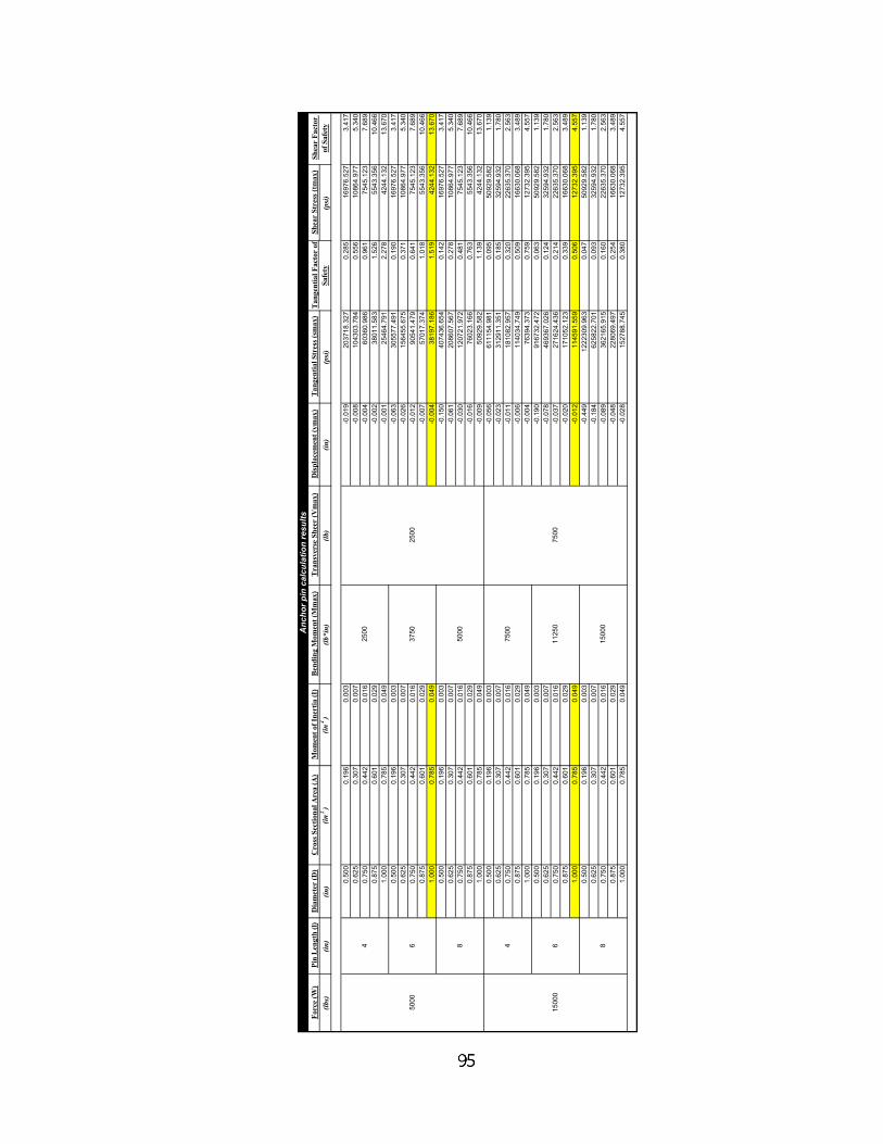
Forc
e (W
)Pi
n L
engt
h (l)
Dia
met
er (D
)C
ross
Sec
tiona
l Are
a (A
)M
omen
t of I
nert
ia (I
)B
endi
ng M
omen
t (M
max
)T
rans
vers
e Sh
eer
(Vm
ax)
Dis
plac
emen
t (ym
ax)
Tan
gent
ial S
tres
s (sm
ax)
Shea
r St
ress
(tm
ax)
(lbs)
(in)
(in)
(in2)
(in4)
(lb*in)
(lb)
(in)
(psi)
(psi)
0.500
0.196
0.003
-0.019
203718.327
0.285
16976.527
3.417
0.625
0.307
0.007
-0.008
104303.784
0.556
10864.977
5.340
0.750
0.442
0.016
-0.004
60360.986
0.961
7545.123
7.689
0.875
0.601
0.029
-0.002
38011.583
1.526
5543.356
10.466
1.000
0.785
0.049
-0.001
25464.791
2.278
4244.132
13.670
0.500
0.196
0.003
-0.063
305577.491
0.190
16976.527
3.417
0.625
0.307
0.007
-0.026
156455.675
0.371
10864.977
5.340
0.750
0.442
0.016
-0.012
90541.479
0.641
7545.123
7.689
0.875
0.601
0.029
-0.007
57017.374
1.018
5543.356
10.466
1.000
0.785
0.049
-0.004
38197.186
1.519
4244.132
13.670
0.500
0.196
0.003
-0.150
407436.654
0.142
16976.527
3.417
0.625
0.307
0.007
-0.061
208607.567
0.278
10864.977
5.340
0.750
0.442
0.016
-0.030
120721.972
0.481
7545.123
7.689
0.875
0.601
0.029
-0.016
76023.166
0.763
5543.356
10.466
1.000
0.785
0.049
-0.009
50929.582
1.139
4244.132
13.670
0.500
0.196
0.003
-0.056
611154.981
0.095
50929.582
1.139
0.625
0.307
0.007
-0.023
312911.351
0.185
32594.932
1.780
0.750
0.442
0.016
-0.011
181082.957
0.320
22635.370
2.563
0.875
0.601
0.029
-0.006
114034.749
0.509
16630.068
3.489
1.000
0.785
0.049
-0.004
76394.373
0.759
12732.395
4.557
0.500
0.196
0.003
-0.190
916732.472
0.063
50929.582
1.139
0.625
0.307
0.007
-0.078
469367.026
0.124
32594.932
1.780
0.750
0.442
0.016
-0.037
271624.436
0.214
22635.370
2.563
0.875
0.601
0.029
-0.020
171052.123
0.339
16630.068
3.489
1.000
0.785
0.049
-0.012
114591.559
0.506
12732.395
4.557
0.500
0.196
0.003
-0.449
1222309.963
0.047
50929.582
1.139
0.625
0.307
0.007
-0.184
625822.701
0.093
32594.932
1.780
0.750
0.442
0.016
-0.089
362165.915
0.160
22635.370
2.563
0.875
0.601
0.029
-0.048
228069.497
0.254
16630.068
3.489
1.000
0.785
0.049
-0.028
152788.745
0.380
12732.395
4.557
8
2500
3750
5000
7500
11250
7500
Tan
gent
ial F
acto
r of
Sa
fety
Shea
r Fa
ctor
of
Saf
ety
15000Anc
hor p
in c
alcu
latio
n re
sults
5000
15000
4 6 8 4 6
2500

DC
+ O
AB
Diagram:
Find: (1) Maximum normal stresses, σmax due to the hole for securing the anchor pin(2) Resultant load on each bolt, Fa,b,c,d(3) Maximum bolt shear stress, τmax(4) Maximum bearing stress, σbear(5) Critical bending stress in the bar, σbend
Minimum distance from hole center to plate edgeh 1.75in:=
Plate thicknesst 0.5in:=
Plate widthw 4.0in:=
Diameter of hole in the plated 1in:=
Max design load on pinF 15000lb:=Given:
Calculation for Anchor Plates
96

n 4:= Number of bolts used
Now, find the primary shear force F' and secondary shear force F"
FprimeVn
:= Fprime 3.75 103× lb=
FDBLprimeMn r⋅
:= FDBLprime 9.621 103× lb=
Adding the two force vectors using the parallelogram rule
φ atan2in3in
:= φ 33.69deg= Angle between F' and r
βAB 90deg φ−:= βAB 56.31deg= Angle between F' and F"
βCD 90deg φ+:= βCD 123.69deg= Angle between F' and F"
Solution: Part (1)
First calculate parameters to look up Kt from Frocht and Hill
dw
0.25=
hw
0.438=
Kt 4.75:=
Next determine the nominal stresses σo and τo
σoF
w d−( ) t⋅:= σo 1 104×
lb
in2=
σmax Kt σo⋅:= σmax 4.75 104×lb
in2=
Part (2): First find the shear force V and moment M about point "O"
V F:= V 1.5 104× lb=
M F 9.25⋅ in:= M 1.387 105× lb in⋅=
r 2in( )2 3in( )2+:= r 3.606 in=
97

dbolt 0.375in:= Nominal diameter of the bolt
Ab dbolt tw⋅:= Ab 0.118 in2= Bearing Area
σbearFA−
Ab:= σbear 1.028− 105×
lb
in2=
Part (5): The critical bending stress acts through bolts A and B
MAB F 7.25⋅ in:= MAB 1.087 105× lb in⋅=
Iplatet 8in( )3⋅12
:= Iplate 21.333 in4=
Iholest dbolt
3⋅
12:= Iholes 2.197 10 3−× in4=
I Iplate 2 Iholes 3 in⋅( )2 t⋅ dbolt⋅ + ⋅−:= I 17.954 in4=
σbendMAB w⋅
I:= σbend 2.423 104×
lb
in2=
FA Fprime2 FDBLprime
2+ 2 Fprime⋅ FDBLprime⋅ cos βAB( )⋅+:= FA 1.211 104× lb=
FB FA:= FB 1.211 104× lb=
FC Fprime2 FDBLprime
2+ 2 Fprime⋅ FDBLprime⋅ cos βCD( )⋅+:= FC 8.161 103× lb=
FD FC:= FD 8.161 103× lb=
Part (3): The bolt used is a flat head bolt with a size of 3/8"-16 x 1" made of steel
As 0.0678in2:= Minor Pitch Diameter Area
τBoltFAAs
:= τBolt 1.786 105×lb
in2=
Part (4): Since the web of the c-channel is thiner than the anchor plate the largest bearing force is due to the pressing of the bolt agianst the web of the c-channel
tw 0.314in:= Web thickness of C6x10.5 channel
98

Please note the naming convention used is: Top Plate is #1Left Channel is #2Right Channel is #3
Diagram:
Yield strength of 1018 HR Steelσyield 32000lb
in2:=
Youngs Modulus for 1018 HR SteelE 30 106⋅lb
in2:=
Height of pin above the top platehpin 4in:=
Height of C6x10.5 channelhc 6in:=
Cross sectional area of C6x10.5 channelAc 3.09in2:=
Overall lenght of structural membersl 96in:=
Thickness of top platetp 0.5in:=
Width of top platewp 6in:=
Design tensile forceFdesign 5000lb:=
Max tensile force based on hydraulicsFmax 15000lb:=
Given:
Calculations for Structural Members
99

Larm 6.438 in=Larm hpin tp hc+( ) ybar− +:=
Calculate the moment produced:
Ix 51.795 in4=Ix Ix.1 Ix.2+ Ix.3+:=
Ix.3 18.686 in4=Ix.3 15.2in4 3.09in2 ybar 3.00in−( )2⋅+:=
Ix.2 18.686 in4=Ix.2 15.2in4 3.09in2 ybar 3.00in−( )2⋅+:=
Ix.1 14.423 in4=Ix.1wp tp
3⋅
123in2( ) 6.25in( ) ybar−
2⋅+:=
Now, find the moment of inertia for the composite beam:
ybar 4.062 in=ybar37.290in3
9.180in2:=
xbar 3 in=xbar27.540in3
9.180in2:=
Solving for the centroids yeilds:
Componant Area xbar ybar xbarA ybarA(in2) (in) (in) (in3) (in3)
1 3.000 3.000 6.250 9.000 18.7502 3.090 0.499 3.000 1.542 9.2703 3.090 5.501 3.000 16.998 9.270
Sums 9.180 N/A N/A 27.540 37.290
First determine the location of the Neutral Axis from the orgin at the lower left corner of the cross section via geometery
Solution: Part (1):
Find: (1) Max deflection angle, θmax(2) Max deflection, ymax(3) Max Stress, σmax(4) Associated Factors of Safety, SF
100
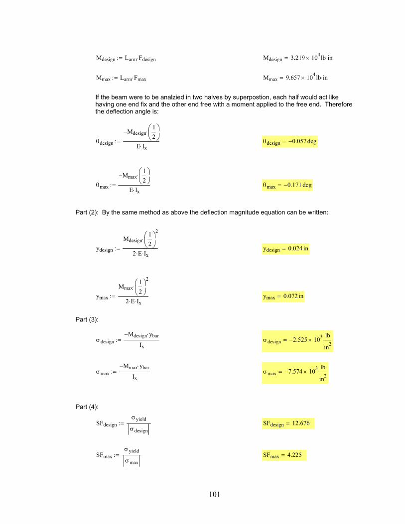
SFmax 4.225=SFmaxσyield
σmax:=
SFdesign 12.676=SFdesignσyield
σdesign:=
Part (4):
σmax 7.574− 103×lb
in2=σmax
Mmax− ybar⋅
Ix:=
σdesign 2.525− 103×lb
in2=σdesign
Mdesign− ybar⋅
Ix:=
Part (3):
ymax 0.072 in=ymax
Mmaxl2
2⋅
2 E⋅ Ix⋅:=
ydesign 0.024 in=ydesign
Mdesignl2
2⋅
2 E⋅ Ix⋅:=
Part (2): By the same method as above the deflection magnitude equation can be written:
θmax 0.171− deg=θmax
Mmax−l2
⋅
E Ix⋅:=
θdesign 0.057− deg=θdesign
Mdesign−l2
⋅
E Ix⋅:=
If the beam were to be analzied in two halves by superpostion, each half would act like having one end fix and the other end free with a moment applied to the free end. Thereforethe deflection angle is:
Mmax 9.657 104× lb in⋅=Mmax Larm Fmax⋅:=
Mdesign 3.219 104× lb in⋅=Mdesign Larm Fdesign⋅:=
101

Hydraulic Schematic:
Max tensile forceFmax 15000lbf:=
Design tensile forceFdes 5000lbf:=
Linear actuator stroke lengthstroke 18in:=
Linear actuator piston diameterbore 2.5in:=
Velocity of the cross headVcross_head 144inmin
:=
Flow output of power packQ 19.8galmin
:=
Maximum pressure output of power packPmax 5000psi:=
Design pressure output of power packPdes 1950psi:=
Given:
Calculations for Hydraulic Parts
102

qFCVmax 3.47hp=qFCVmax Pfcmax QLA⋅:=
qFCVdes 1.663hp=qFCVdes Pfcdes QLA⋅:=
qFCVman 0.268hp=qFCVman Pfcman QLA⋅:=
Pfcmax 1.944 103× psi=Pfcmax Pmax PLAmax−:=
Pfcdes 931.408psi=Pfcdes Pdes PLAdes−:=
Pfcman 150psi:=
Part (3): Since the flow remains constant calculate the pressure loss across the FCV (Pfc)
PLAmax 3.056 103× psi=PLAmaxFmax
πbore2
2⋅
:=
PLAdes 1.019 103× psi=PLAdesFdes
πbore2
2⋅
:=
QLA 3.06galmin
=QLA Vcross_head π⋅bore2
2⋅:=
Part (2):
Whpmax 57.75hp=Whpmax Pmax Q⋅:=
Whpdes 22.523hp=Whpdes Pdes Q⋅:=
Solution: Part (1)
Find: (1) Horsepower output of power pack(2) Flow/Pressure requirements of linear actuator (LA)(3-8) Pressure loss, flow reductions, heat sources from:
(3) Flow Control valve (FCV)(4) Load Check valve (LCV)(5) Directional Control valve (DCV)(6) Quick-Disconnects (QD)(7) Selector valve (SV)(8) All lines and hoses
(9) Total estimated losses
103

Now the head loss can be calculated using the Darcy-Wabaush Equation:
f 0.037=f0.3164
Nr0.25
:=
Since the Rynolds number is greater than 4000 the flow is considered to be turbulent. This means the friction factor for the hose is given by the Blasius equation:
Nr 5.149 103×=Nr7740 6.65⋅ 0.5⋅
4.998:=
Velocity of the oil in the hoseVflQLA
πdID
2
4⋅
:=
The kinematic viscosity of oilν 665stokes:=
Inside diameter of the hosedID 0.5in:=
Part (8): Most of the pressure drop will be in the fifty foot sections of hose! So, first compute the Rynolds Number:
qSV 5.355 10 3−× hp=qSV PSV QLA⋅:=
PSV 3psi:=
Part (7): From the manufacturer the pressure drop at the design flow rate is:
qQD 5.355 10 3−× hp=qQD PQD QLA⋅:=
PQD 3psi:=
Part (6): From the manufacturer the pressure drop at the design flow rate is:
qDCV 3.57 10 3−× hp=qDCV PDCV QLA⋅:=
PDCV 2psi:=
Part (5): From the manufacturer the pressure drop at the design flow rate is:
qLCV 8.925 10 3−× hp=qLCV PLCV QLA⋅:=
PLCV 5psi:=
Part (4): From the manufacturer the pressure drop across the LCV is:
104
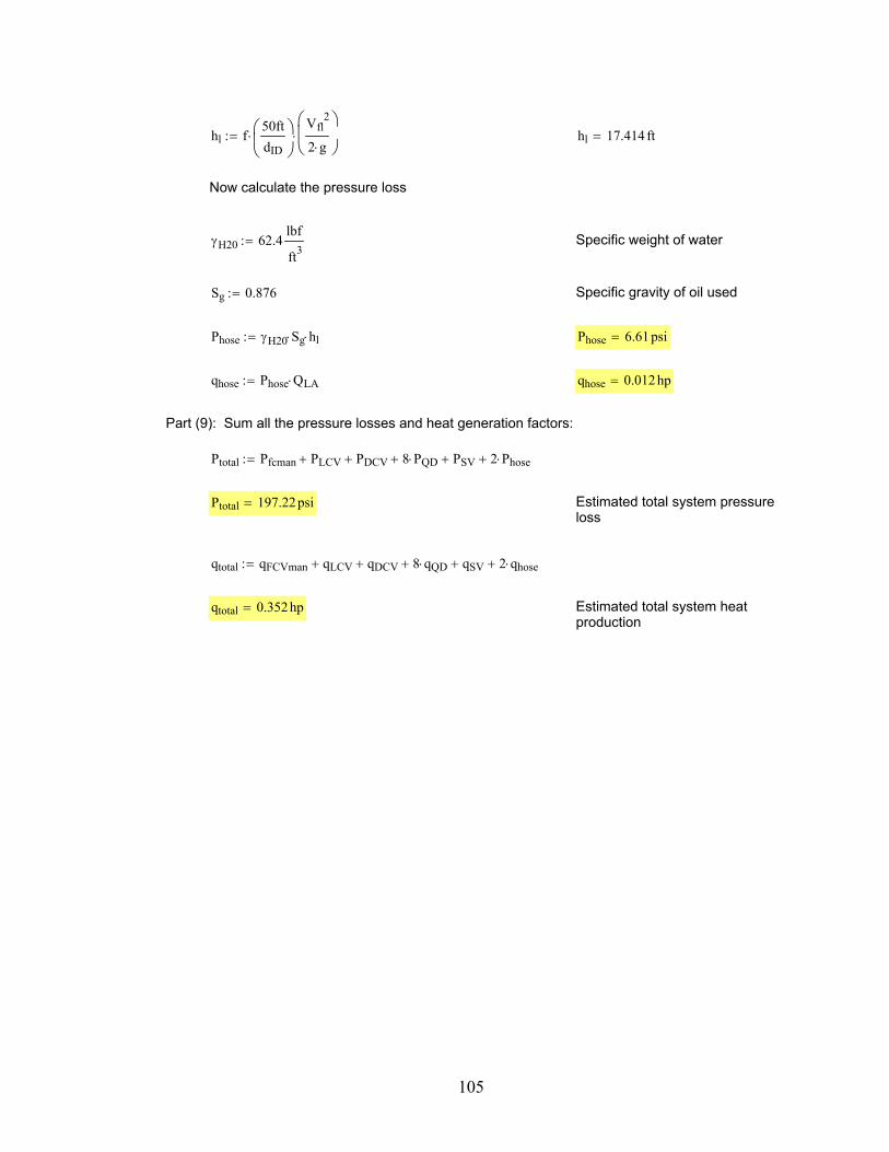
Estimated total system heat production
qtotal 0.352hp=
qtotal qFCVman qLCV+ qDCV+ 8 qQD⋅+ qSV+ 2 qhose⋅+:=
Estimated total system pressure loss
Ptotal 197.22psi=
Ptotal Pfcman PLCV+ PDCV+ 8 PQD⋅+ PSV+ 2 Phose⋅+:=
Part (9): Sum all the pressure losses and heat generation factors:
qhose 0.012hp=qhose Phose QLA⋅:=
Phose 6.61psi=Phose γH20 Sg⋅ hl⋅:=
Specific gravity of oil usedSg 0.876:=
Specific weight of waterγH20 62.4lbf
ft3:=
Now calculate the pressure loss
hl 17.414 ft=hl f50ftdID
⋅Vfl2
2 g⋅
⋅:=
105

106
APPENDIX B:
AutoCAD Fabrication Drawings

107

108

109

110

111
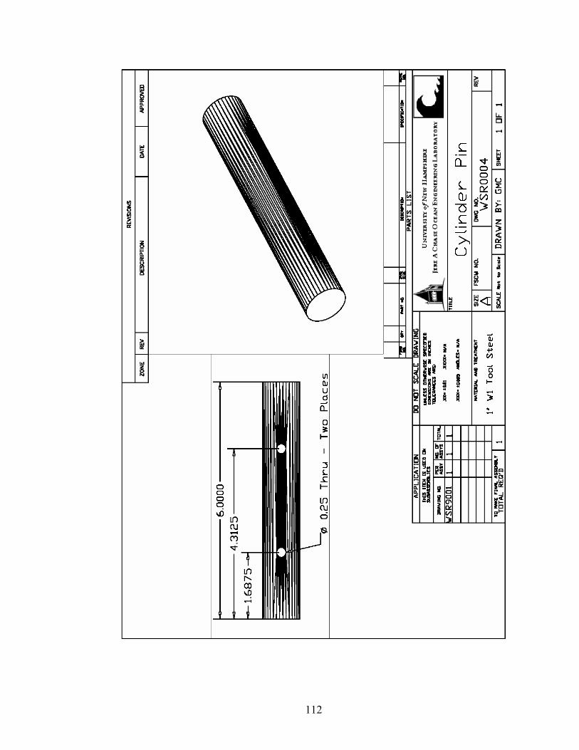
112

113

114
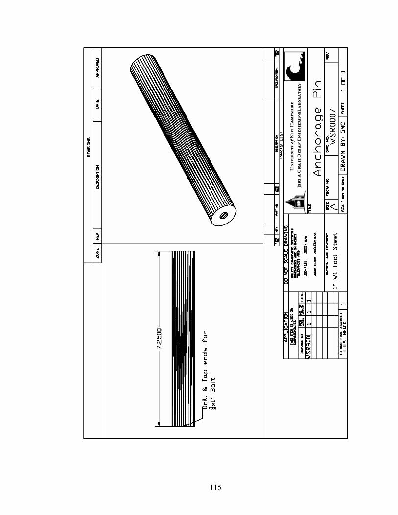
115

116

117

118
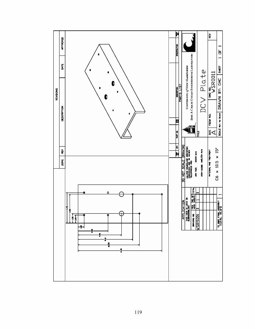
119

120
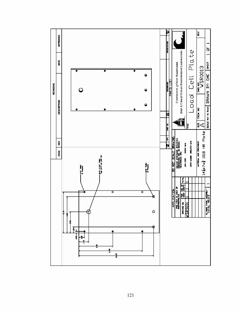
121

122
APPENDIX C:
MatLab Code

123
%%%%%%%%%%%%%%%%%%%%%%%%%%%%%%%%%%%%%%%%%%%%%%%%%% %WSR_main processes the raw data from rope breaking experiments one at a time or in a % % bundle. % % WSR_main takes in four arguments % % (1) The first is the Synchro file containing the LANC info and Load Cell data % % (2) The right or left camera image text file as output by Ropemovie program and % % automatically loads both the left and right % % (3) The last input file is the excel file containing the sample S/N with the starting % % frame for both the left and right video captures % % WSR_main outputs a varity of graphs including the raw engineering stress-strain, % % elongation and delta elongation vs sample #, stress and delta stress verses sample #, % % and various curve fits for the data. % % WSR_main calls the following functions: % % (1) Datamatch.m % % (2) LANCadj.m % % (3) FitIndicies.m % % (4) WSRCurveFit.m % % (5) WSRStats.m % % (6) PlotStruct.m % % % % By Glenn McGillicuddy % % Date: 8/25/05 % %%%%%%%%%%%%%%%%%%%%%%%%%%%%%%%%%%%%%%%%%%%%%%%%%% close all; clear all; clc; numfiles = 1; %Number of files to process(files must be listed in the reference file) limit = 2; %Number of Standard deviations to include in the setting of the fit limits ITp = 200*0.375^2; %Initial Tension based on diameter to calculate the starting point of all fits %strand_dia = 0.165; %Strand diameter of the rope under analysis % Prompt the user for the starting files and directories [synfile,synpath] = uigetfile('C:\MATLAB6p5\work\WSR\Data\*.syn',... 'Select the first SYNCRO file to be processed'); [imagefile,imagepath] = uigetfile('C:\MATLAB6p5\work\WSR\Data\*.txt',... 'Select the associated IMAGE text file (Right or Left)'); [reffile,refpath] = uigetfile('C:\MATLAB6p5\work\WSR\Data\*.txt',... 'Select the TEXT file that contains the frame references'); check = strcmp(synfile(1,end-8:end-4),imagefile(1,1:5)); if check == 0 error('Syncro file does not match specified Image text file') end clear check; % Load the Text reference file for the starting points of the Video captures. [sample, LcamM, LcamS, LcamF, RcamM, RcamS, RcamF] = textread(strcat(refpath,reffile),... '%5c %*2c %2c %2c %2c %*2c %2c %2c %2c %*6c'); Lcam_cap = strcat('0:', LcamM, ':', LcamS, ':', LcamF); Rcam_cap = strcat('0:', RcamM, ':', RcamS, ':', RcamF); clear LcamM LcamS LcamF RcamM RcamS RcamF; % Load the Synchro file and the Ropemovie text files (for loop iterates for the specified number of

124
% files) for m = 1:numfiles if m == 1 [Lcam, Rcam, Data_raw(:,1)] = textread(strcat(synpath,synfile),... '%*26c %10c %*5c %10c %*10c %f %*26c'); [Lcam_image(:,1), Lcam_image(:,2), Lcam_image(:,3), Lcam_image(:,4)] =... textread(strcat(imagepath,imagefile(1:end-5),'L.txt'),'%u %f %f %f'); [Rcam_image(:,1), Rcam_image(:,2), Rcam_image(:,3), Rcam_image(:,4)] =... textread(strcat(imagepath,imagefile(1:end-5),'R.txt'),'%u %f %f %f'); else file_index = strmatch(synfile(1,end-8:end-4),sample, 'exact') + 1; synfile = strcat(synfile(1,1:end-9),sample(file_index,:),'.syn'); imagefile = strcat(sample(file_index,:), 'L.txt'); check = strcmp(synfile(1,end-8:end-4),imagefile(1,1:5)); if check == 0 error('Syncro file does not match specified Image text file') end clear check file_index; [Lcam, Rcam, Data_raw(:,1)] = textread(strcat(synpath,synfile),... '%*26c %10c %*5c %10c %*10c %f %*26c'); [Lcam_image(:,1), Lcam_image(:,2), Lcam_image(:,3), Lcam_image(:,4)] =... textread(strcat(imagepath,imagefile(1:end-5),'L.txt'),'%u %f %f %f'); [Rcam_image(:,1), Rcam_image(:,2), Rcam_image(:,3), Rcam_image(:,4)] =... textread(strcat(imagepath,imagefile(1:end-5),'R.txt'),'%u %f %f %f'); end % Down sample the data such that there is only one data point per LANC change rec_index = max(strmatch(Lcam(1,:),Lcam)) + 1; ovr_samp = strncmp(Lcam(rec_index,:), Lcam(rec_index+1,:),10); if ovr_samp == 0 LC_data = Data_raw; cam_LANC(:,1:10) = Lcam; cam_LANC(:,12:21) = Rcam; else [row col] = size(Lcam); datapts = fix(row/9); index = 1; for n = 1:datapts LC_data(index,:) = Data_raw((n*9),:); cam_LANC(index,1:10) = Lcam((n*9),:); cam_LANC(index,12:21) = Rcam((n*9),:); index = index + 1; end end clear Data_raw Lcam Rcam row col datapts index n rec_index ovr_samp; % Match the image data up with the load cell data using the LANC info and the reference text file. Lcam_strt = Lcam_cap(strmatch(synfile(1,end-8:end-4),sample, 'exact'),:); Lcam_strt = LANCadj(Lcam_strt,Lcam_image(1,1)); Rcam_strt = Rcam_cap(strmatch(synfile(1,end-8:end-4),sample, 'exact'),:); Rcam_strt = LANCadj(Rcam_strt,Rcam_image(1,1));

125
Aligned_data = Datamatch(Lcam_strt,Rcam_strt,cam_LANC,LC_data,Lcam_image, Rcam_image); clear Lcam_strt Rcam_strt ans cam_LANC; % Now apply corrections to the Load cell data Corrected_data(:,1) = (Aligned_data(:,1)+0.0003)/0.0033; test_stats = max(Corrected_data(:,1)); test_stats(1,2) = mean((LC_data(end-10:end,1)+0.0003)/0.0033); % Convert transition point from a pixel to an actual distance using the ruler of the image file. Aligned_data(:,4:5) = 0; for n=1:length(Aligned_data(2:end,1)) Aligned_data(n+1,4) = (Aligned_data(n,2) - Aligned_data(n+1,2)) + Aligned_data(n,4); Aligned_data(n+1,5) = (Aligned_data(n,3) - Aligned_data(n+1,3)) + Aligned_data(n,5); end clear n; ruler = 2/2.54; %Stripes on ruler are 2cm wide convert to inches test_stats(2,1) = ruler/(mean(Lcam_image(:,4))); %Determine the inches per pixels test_stats(2,2) = std(Lcam_image(:,4)); Corrected_data(:,2) = Aligned_data(:,4) * test_stats(2,1); test_stats(3,1) = ruler/(mean(Rcam_image(:,4))); test_stats(3,2) = std(Rcam_image(:,4)); Corrected_data(:,3) = Aligned_data(:,5) * test_stats(3,1); % Compute the Engineering stress-strain for the data points and plot the unfitted data Lo = 12; %Original gauge length Ao = .11044; %3*((pi*(strand_dia^2))/4); %Cross-sectional area of WSR s = Corrected_data(:,1) / Ao; e = (Corrected_data(:,2)-Corrected_data(:,3))/Lo; figure(1) title('Engineering Stress-Strain'); xlabel('Strain ( in / in )'); ylabel('Stress ( lbs / in^2 )'); grid on hold on plot(e,s,'bo','Tag',synfile(1,end-8:end-4)); % Call function to determine indicies for curve fitting [DervData, indicies] = FitIndicies(limit,ITp,synfile,Ao,e,s); % Fit a curve to the stress-strain data points [s_fit, e_fit] = WSRCurveFit(e,s,DervData,indicies,synfile); % Store the data processed_data(m) = struct('Experiment', synfile(1,end-8:end-4), 'Stress', s, 'Derivative_Stress',... DervData, 'Strain', e, 'Test_Stats', test_stats, 's_Curve_Fits', s_fit, 'e_Curve_Fits', e_fit,... 'Curve_Indicies', indicies); clear Aligned_data Corrected_data DervData LC_data Lcam_image Lo Rcam_image e fit...

126
indicies ruler s test_stats; end clear Lcam_cap Rcam_cap imagefile imagepath m n numfiles reffile refpath sample synfile synpath; %Determine the stats for the curve fits [s_avg_val, s_avg_val_std, s_avg_fit, s_avg_fit_std] = WSRStats(processed_data, 's'); [e_avg_val, e_avg_val_std, e_avg_fit, e_avg_fit_std] = WSRStats(processed_data, 'e'); % Fit the average elongation data s = [0.1,0.5,0.9]'*s_avg_val(4,3); for n = 1:length(processed_data) e(n,1) = (polyval(processed_data(n).e_Curve_Fits(1,:),s(1))); e(n,2) = processed_data(n).e_Curve_Fits(2,2)+processed_data(n).e_Curve_Fits(2,3)*s(2); e(n,3) = polyval(processed_data(n).e_Curve_Fits(3,:),s(3)); end e_mean = mean(e)*12; e_std = std(e*12); % Call a plotting function to produce the plots PlotStruct(s_avg_fit,s_avg_fit_std,s_avg_val,s_avg_val_std,processed_data); strcat('Average Mechanical Settling Point is: ', num2str(s_avg_val(2,3)*Ao), ' lbs') strcat('Average Yield Point is: ', num2str(s_avg_val(3,3)*Ao), ' lbs') strcat('Average Ultimate Tensile Point is:', num2str(s_avg_val(4,3)*Ao), ' lbs') strcat('Average Young’s Modulus is: ', num2str(s_avg_fit(2,3)),' psi')

127
function [Aligned_data] = Datamatch(Lcam_strt,Rcam_strt,cam_LANC,LC_data,Lcam_image, Rcam_image) %%%%%%%%%%%%%%%%%%%%%%%%%%%%%%%%%%%%%%%%%%%%%%%%%% %Datamatch complies the Load cell and the Left and Right Transition pixels into one array % % The first two input arguments are character strings that represent the Left and Right % % starting LANCs from the image processing % % The third input argument is the Left and Right LANC strings from the SYNCRO file % % The fourth input argument is a double array which represents the load cell data from % % the SYNCRO file % % The fifth and sixth input parameters are double arrays containing the results of the % % image processing (Relative Frame#, Transition Pixel, Robustness, and Ruler Pixel) % % The function outputs a double array containing the Load cell data and the transition % % pixels of the Left and Right cameras % % % % By Glenn McGillicuddy % % Date: 8/20/05 % %%%%%%%%%%%%%%%%%%%%%%%%%%%%%%%%%%%%%%%%%%%%%%%%%% % Matching the Left camera LANC from SYNCRO data and the image processing starting point and % returing the index Lcam_index = strmatch(Lcam_strt,cam_LANC(:,1:10), 'exact'); tf = isempty(Lcam_index); if tf == 1 Lcam_strt = LANCadj(Lcam_strt,1); Lcam_index = strmatch(Lcam_strt,cam_LANC(:,1:10), 'exact'); tf = isempty(Lcam_index); if tf == 1 Aligned_data = 0; error('Can not match up LANC data and Left camera frame starting point!!') end clear tf; Lcam_image(1,:) = []; end clear tf; % Matching the Right camera LANC from SYNCRO data and the image processing starting point and % returning the index Rcam_index = strmatch(Rcam_strt,cam_LANC(:,12:21), 'exact'); tf = isempty(Rcam_index); if tf == 1 Rcam_strt = LANCadj(Rcam_strt,1); Rcam_index = strmatch(Rcam_strt,cam_LANC(:,12:21), 'exact'); tf = isempty(Rcam_index); if tf == 1 Aligned_data = 0; error('Can not match up LANC data and Right camera frame starting point!!') end clear tf; Rcam_image(1,:) = []; end clear tf; % Truncate the start of the image data file that starts first such that the Left and Right

128
% cameras start at the same point in the SYNCRO file if Lcam_index > Rcam_index abs_index = Lcam_index; Rcam_image(1:((Lcam_index - Rcam_index)*2),:) = []; elseif Rcam_index > Lcam_index abs_index = Rcam_index; Lcam_image(1:((Rcam_index - Lcam_index)*2),:) = []; else abs_index = Lcam_index; end % Combining the Load Cell data and the Left and Right camera transition tracking data % Remembering that the image data is at 30Hz and the Syncro data is at 15Hz so, you % must down sample the image data Aligned_data = LC_data(abs_index:end,1); if length(Lcam_image) >= length(Rcam_image) i = fix(length(Rcam_image)/2); else i = fix(length(Lcam_image)/2); end Aligned_data(1,2) = Lcam_image(1,2); Aligned_data(1,3) = Rcam_image(1,2); for j = 1:i-1 Aligned_data(j+1,2) = Lcam_image(((j*2)+1),2); Aligned_data(j+1,3) = Rcam_image(((j*2)+1),2); end % Now remove all data points without any transition data if length(Aligned_data) > i Aligned_data(i+1:end,:) = []; end clear Lcam_index Rcam_index Lcam_strt Rcam_strt abs_index i j;

129
function [cam_index] = LANCadj(cam_index,offset) %%%%%%%%%%%%%%%%%%%%%%%%%%%%%%%%%%%%%%%%%%%%%%%%%% %LANCadj changes the LANC string % % LANCadj takes in two arguments % % The first argument is the character array containing the LANC string to be adjusted % % The last argument is a 1x1 double array representing the number of frames to % % offset the LANC string by % % This function outputs a character array that represents the H:MM:SS:FF of the adjusted % % LANC string % % % % By Glenn McGillicuddy % % Date: 8/20/05 % %%%%%%%%%%%%%%%%%%%%%%%%%%%%%%%%%%%%%%%%%%%%%%%%%% % Convert the strings to numbers and add the offset to the frame number camM = str2num(cam_index(1,3:4)); camS = str2num(cam_index(1,6:7)); camF = str2num(cam_index(1,9:10)) + offset; % Check to ensure that values are in the correct quanities if camF >= 30 camS = camS + fix(camF/30); if camS >= 60 camM = camM + fix(camS/60); camS = camS - (fix(camS/60)*60); end camF = camF - (fix(camF/30)*30); end % Convert the adjusted numbers back to a character string if camF <= 9 camF = strcat('0', num2str(camF)); else camF = num2str(camF); end if camS <= 9 camS = strcat('0', num2str(camS)); else camS = num2str(camS); end if camM <= 9 camM = strcat('0', num2str(camM)); else camM = num2str(camM); end % Form a character string in the H:MM:SS:FF format cam_index = strcat('0:', camM, ':', camS, ':', camF); clear camM camS camF;

130
function [DervData, indicies] = FitIndicies(limit,ITp,synfile,Ao,e,s) %%%%%%%%%%%%%%%%%%%%%%%%%%%%%%%%%%%%%%%%%%%%%%%%%% %FitIncicies determines the linear indices of the mechanical and strain hardening regions % % The first input argument is the number of STD to define the allowable data spread when % % determining the indices % % The second input argument is the calculated initial tension based on the CI guidelines % % The third input argument is the SYNCRO file name % % The fourth input parameter is the cross sectional area of the rope % % The fifth and sixth input arguments are the corrected strain and stress data % % The function outputs a double array containing the derivative of stress data and a % % matrix containing the indices for the start, mechanical, yield, and UTS along % % with the stress and strain values at these indices % % % % By Glenn McGillicuddy % % Date: 09/01/05 % %%%%%%%%%%%%%%%%%%%%%%%%%%%%%%%%%%%%%%%%%%%%%%%%%% % Find the starting point in the stress data that exceeds the Initial Tension criterion strt = find(s >= ITp/Ao); % Determine the first derivative of stress and plot for n = 1:length(s)-1 ds(n,1) = s(n+1,1)-s(n,1); if ds(n,1) < 0 ds(n,1) = 0; end end % Detect and note any data spikes dsmean = mean(ds(20:60,1)); k = 1; spike_index = []; for n = 10:length(ds)-10 if ds(n,1) > dsmean+150 || ds(n,1) < dsmean-150 spike_index(k,1) = n; k = k + 1; end end % Remove any data spikes by placing the values at the mean value clear k n; if isempty(spike_index) 'No data spikes within set limits' else for n = 1:length(spike_index) ds(spike_index(n,1),1) = dsmean; end end % Run a boxcar filter forwards and backwards to smooth the data and plot windowSize = 5;

131
dsfilt = filtfilt(ones(1,windowSize)/windowSize,1,ds); figure(2) title('First Derivative of Stress'); xlabel('Linear Index Number'); ylabel('d\sigma'); grid on hold on plot(ds,'bo','Tag',synfile(1,end-8:end-4)) plot(dsfilt,'r*--','Tag',strcat(synfile(1,end-8:end-4),' Filtered')) % Determine the second derivative of stress, filter, and plot for r = 1:length(dsfilt)-1 d2s(r,1) = dsfilt(r+1,1) - dsfilt(r,1); end d2sfilt = filtfilt(ones(1,windowSize)/windowSize,1,d2s); d2smean = mean(d2sfilt(20:60,1)); d2sstd = std(d2sfilt(20:60,1)); figure(3) title('Second Derivative of Stress'); xlabel('Linear Index Number'); ylabel('d^2\sigma'); grid on hold on plot(d2s,'bo','Tag',synfile(1,end-8:end-4)) plot(d2sfilt,'r*--','Tag',strcat(synfile(1,end-8:end-4),' Filtered')) % Working from index of 20 back to one find the point at which the 2nd derivative % of stress is outside of plus or minus one two standard derivations of the mean i = 20; k = 0; while k == 0 && i > 0 if d2sfilt(i-1,1) <= d2smean+(limit*d2sstd) && d2sfilt(i-1,1) >= d2smean-(limit*d2sstd) i = i-1; else k = 1; i_mech = i; end if i == 1 'WARNING: No Mechanical limit Found' i_mech = 20; end end % Working from index of 60 forward to end of data find the point at which the 2nd % derivative of stress is outside of plus or minus one two standard derivations of the mean i = 60; k = 0; while k == 0 && i < length(d2sfilt) if d2sfilt(i+1,1) <= d2smean+(limit*d2sstd) && d2sfilt(i+1,1) >= d2smean-(limit*d2sstd) i = i+1;

132
else k = 1; i_yield = i; end if i == length(d2sfilt)-1 'WARNING: No Yield Point Found' i_yield = 75; end end % Find the ultimate breaking strength and the associated index [UTS i_UTS] = max(s); % Plot the indicies figure(3) plot(i_mech,[-20:0.1:20], 'm') plot(i_yield,[-20:0.1:20], 'm') figure(2) plot(i_mech,[150:0.1:250], 'm') plot(i_yield,[150:0.1:250], 'm') % Format the data to be retuned to the calling program indicies(1,1) = strt(2); indicies(1,2) = e(strt(2)); indicies(1,3) = s(strt(2)); indicies(2,1) = i_mech; indicies(2,2) = e(i_mech); indicies(2,3) = s(i_mech); indicies(3,1) = i_yield; indicies(3,2) = e(i_yield); indicies(3,3) = s(i_yield); indicies(4,1) = i_UTS; indicies(4,2) = e(i_UTS); indicies(4,3) = s(i_UTS); DervData(:,1) = dsfilt; DervData(2:end,2) = d2sfilt; clear UTS ans d2s d2filt d2smean d2sstd ds dsfilt dsmean i i_UTS i_mech i_yield k... limit r spike_index strt windowSize;

133
function [s_fit, e_fit] = WSRCurveFit(e,s,DervData,indicies,synfile) %%%%%%%%%%%%%%%%%%%%%%%%%%%%%%%%%%%%%%%%%%%%%%%%%% %WSRCurveFit determines calculates a number of piecewise fit for each of the data plots % % The first and second input arguments are the corrected strain and stress data % % The third input argument is derivative data from FitIndicies.m % % The fourth input parameter is the matrix of indices from FitIndicies.m % % The fifth input argument is the name of the file under investigation % % The function outputs two double array containing the associated fits for the stress and % % strain data for the engineering stress-strain, 1st derivative of stress and the % % 2nd derivative of stress % % % % By Glenn McGillicuddy % % Date: 09/01/05 % %%%%%%%%%%%%%%%%%%%%%%%%%%%%%%%%%%%%%%%%%%%%%%%%%% % Break out the indices and data strt = indicies(1,1); i_mech = indicies(2,1); i_yield = indicies(3,1); i_UTS = indicies(4,1); dsfilt = DervData(:,1); d2sfilt = DervData(2:end,2); % Perform a linear fit to the second derivative between the extracted mech and yield points d2sfit = robustfit([i_mech:1:i_yield]',d2sfilt(i_mech:i_yield,1)); % Now find the approach slope, max value, and decending slope of the first derivative k = 0; n = 20; while k == 0 && n < i_yield if d2sfilt(n,1) + d2sfilt(n+1,1) <= 0 zerocross = n; k = 1; end n = n + 1; end dsappfit = robustfit([i_mech:1:zerocross]', dsfilt(i_mech:zerocross,1)); dsdecfit = robustfit([zerocross:1:i_yield]', dsfilt(zerocross:i_yield,1),1); dsinter = (dsappfit(1)-dsdecfit(1))/(dsdecfit(2)-dsappfit(2)); % Now fit the raw Stress-Strain data using the mech and yield indices mechreg_s = polyfit(e(strt:20),s(strt:20),2); mechreg_e = polyfit(s(strt:20),e(strt:20),2); elasreg_s = robustfit(e(i_mech:i_yield),s(i_mech:i_yield)); elasreg_e = robustfit(s(i_mech:i_yield),e(i_mech:i_yield)); strnhard_s = polyfit(e(i_yield:i_UTS),s(i_yield:i_UTS),2); strnhard_e = polyfit(s(i_yield:i_UTS),e(i_yield:i_UTS),2); % Plot these fits on the associated figures

134
figure(1) f1 = polyval(mechreg,e(1:i_mech)); f2 = elasreg(1)+elasreg(2)*e(i_mech:i_yield); f3 = polyval(strnhard,e(i_yield:i_UTS)); plot(e(1:i_mech),f1,'g','Tag',strcat(synfile(1,end-8:end-4),' Mechanical')) plot(e(i_mech:i_yield),f2,'r','Tag',strcat(synfile(1,end-8:end-4),' Elastic')) plot(e(i_yield:i_UTS),f3,'c','Tag',strcat(synfile(1,end-8:end-4),' Strain Hardened')) figure(2) plot([1:1:zerocross+10]',dsappfit(1)+dsappfit(2)*[1:1:zerocross+10]','k-','Tag',... strcat(synfile(1,end-8:end-4),' Approach')) plot([zerocross-10:1:length(dsfilt)]',dsdecfit(1)+dsdecfit(2)*[zerocross-10:1:length(dsfilt)]',... 'k-','Tag',strcat(synfile(1,end-8:end-4),' Decending')) plot(dsinter,dsdecfit(1)+dsdecfit(2)*dsinter,'c*','Tag',strcat(synfile(1,end-8:end-4),... 'Intersection')) figure(3) plot([1:1:length(d2sfilt)]',d2sfit(1)+d2sfit(2)*[1:1:length(d2sfilt)]','k-','Tag',... strcat(synfile(1,end-8:end-4),' Area Slope')) % Format the data to be retuned to to the calling program s_fit(1,:) = mechreg_s; s_fit(2,2:3) = elasreg_s'; s_fit(3,:) = strnhard_s; s_fit(4,2:3) = dsappfit'; s_fit(5,2:3) = dsdecfit'; s_fit(6,3) = dsinter; s_fit(7,2:3) = d2sfit'; s_fit(8,3) = zerocross; e_fit(1,:) = mechreg_e; e_fit(2,2:3) = elasreg_e'; e_fit(3,:) = strnhard_e; e_fit(4,2:3) = dsappfit'; e_fit(5,2:3) = dsdecfit'; e_fit(6,3) = dsinter; e_fit(7,2:3) = d2sfit'; e_fit(8,3) = zerocross; clear d2sfilt d2sfit dsappfit dsdecfit dsfilt dsinter elasreg f1 f2 f3 i_UTS i_mech... i_yield k mechreg n strnhard strt zerocross

135
function [avg_val, avg_val_std, avg_fit, avg_fit_std] = WSRStats(processed_data, type); %%%%%%%%%%%%%%%%%%%%%%%%%%%%%%%%%%%%%%%%%%%%%%%%%% %WSRStats determines the statistical parameters associated with the fits in each replicate % % The first input argument is the struct containing all the processed data % % The second input argument is a character that determines what fits are analyzed (stress % % or strain). % % The function outputs four double arrays containing the mean and standard deviations % % of the values associated with the fit indices. It also outputs the mean and % % standard deviations of the fits % % % % By Glenn McGillicuddy % % Date: 09/01/05 % %%%%%%%%%%%%%%%%%%%%%%%%%%%%%%%%%%%%%%%%%%%%%%%%%% % Determine the average mechanical settling point, yield point, and ultimate tensile strength for i = 1:length(processed_data) i_strt(i,1:3) = processed_data(i).Curve_Indicies(1,1:3); i_mech(i,1:3) = processed_data(i).Curve_Indicies(2,1:3); i_yield(i,1:3) = processed_data(i).Curve_Indicies(3,1:3); i_UTS(i,1:3) = processed_data(i).Curve_Indicies(4,1:3); mech_fit(i,1:3) = eval(strcat('processed_data(i).',type,'_Curve_Fits(1,1:3)')); elas_fit(i,1:3) = eval(strcat('processed_data(i).',type,'_Curve_Fits(2,1:3)')); hard_fit(i,1:3) = eval(strcat('processed_data(i).',type,'_Curve_Fits(3,1:3)')); appr_fit(i,1:3) = eval(strcat('processed_data(i).',type,'_Curve_Fits(4,1:3)')); dec_fit(i,1:3) = eval(strcat('processed_data(i).',type,'_Curve_Fits(5,1:3)')); inter_fit(i,1:3) = eval(strcat('processed_data(i).',type,'_Curve_Fits(6,1:3)')); d2s_fit(i,1:3) = eval(strcat('processed_data(i).',type,'_Curve_Fits(7,1:3)')); zcross_fit(i,1:3) = eval(strcat('processed_data(i).',type,'_Curve_Fits(8,1:3)')); load(i,1) = processed_data(i).Test_Stats(1,1); end % Organize the data to be transferred back to calling program avg_val(1,1:3) = mean(i_strt); avg_val(2,1:3) = mean(i_mech); avg_val(3,1:3) = mean(i_yield); avg_val(4,1:3) = mean(i_UTS); avg_val(1:4,1) = round(avg_val(1:4,1)); avg_val_std(1,1:3) = std(i_strt); avg_val_std(2,1:3) = std(i_mech); avg_val_std(3,1:3) = std(i_yield); avg_val_std(4,1:3) = std(i_UTS); avg_fit(1,1:3) = mean(mech_fit); avg_fit(2,1:3) = mean(elas_fit); avg_fit(3,1:3) = mean(hard_fit); avg_fit(4,1:3) = mean(appr_fit); avg_fit(5,1:3) = mean(dec_fit); avg_fit(6,1:3) = mean(inter_fit); avg_fit(7,1:3) = mean(d2s_fit); avg_fit(8,1:3) = round(mean(zcross_fit));

136
avg_fit_std(1,1:3) = std(mech_fit); avg_fit_std(2,1:3) = std(elas_fit); avg_fit_std(3,1:3) = std(hard_fit); avg_fit_std(4,1:3) = std(appr_fit); avg_fit_std(5,1:3) = std(dec_fit); avg_fit_std(6,1:3) = std(inter_fit); avg_fit_std(7,1:3) = std(d2s_fit); avg_fit_std(8,1:3) = std(zcross_fit);

137
function PlotStruct(avg_fit,avg_fit_std,avg_val,avg_val_std,processed_data); %%%%%%%%%%%%%%%%%%%%%%%%%%%%%%%%%%%%%%%%%%%%%%%%%% %PlotStruct graphs the corrected data along with the fits and their confidence intervals % % The first four input arguments are the parameters output from WSRStats.m % % The fifth input parameter structure containing the processed data % % % % By Glenn McGillicuddy % % Date: 09/01/05 % %%%%%%%%%%%%%%%%%%%%%%%%%%%%%%%%%%%%%%%%%%%%%%%%%% % Plot the raw data for the Engineering Stress-Strain, delta stress, and delta2 stress figure(1) axis([0 0.3 0 28000]) title('Engineering Stress-Strain'); xlabel('Strain ( in / in )'); ylabel('Stress ( lbs / in^2 )'); box on grid on hold on figure(2) title('First Derivative of Stress'); xlabel('Linear Index Number'); ylabel('ds'); box on grid on hold on figure(3) title('Second Derivative of Stress'); xlabel('Linear Index Number'); ylabel('d^2 s'); box on grid on hold on for n =1:length(processed_data) figure(1) plot(processed_data(n).Strain(avg_val(1,1):end),processed_data(n).Stress(avg_val(1,1):end),... 'bo','Tag',processed_data(n).Experiment); figure(2) plot(processed_data(n).Derivative_Stress(:,1),'bo','Tag',processed_data(n).Experiment); figure(3) plot(processed_data(n).Derivative_Stress(2:end,2),'bo','Tag',processed_data(n).Experiment); end %Create an array of strain values in order to plot the fits e = 0:avg_val(4,2)/(avg_val(4,1)+10):avg_val(4,2); % Evaluate the average fit values based on the above stain matrix f1 = polyval(avg_fit(1,:),e(1:avg_val(2,1))); f2 = avg_fit(2,2)+avg_fit(2,3)*e(avg_val(2,1):avg_val(3,1)); f3 = polyval(avg_fit(3,:),e(avg_val(3,1):end));

138
f4 = avg_fit(4,2)+avg_fit(4,3)*[1:1:avg_fit(8,3)+10]'; f5 = avg_fit(5,2)+avg_fit(5,3)*[avg_fit(8,3)-10:1:avg_val(4,1)]'; f6 = avg_fit(5,2)+avg_fit(5,3)*avg_fit(6,3); f7 = avg_fit(7,2)+avg_fit(7,3)*[1:1:avg_val(4,1)]'; % Compute the upper 95% Confidence Interval f1u = f1 + (1.96*(avg_fit_std(1,3)/sqrt(length(processed_data)))); f2u = f2 + (1.96*(avg_fit_std(2,3)/sqrt(length(processed_data)))); f3u = f3 + (1.96*(avg_fit_std(3,3)/sqrt(length(processed_data)))); f4u = f4 + (1.96*(avg_fit_std(4,2)/sqrt(length(processed_data)))); f5u = f5 + (1.96*(avg_fit_std(5,2)/sqrt(length(processed_data)))); f6u = f6 + (1.96*(avg_fit_std(6,3)/sqrt(length(processed_data)))); f7u = f7 + (1.96*(avg_fit_std(7,2)/sqrt(length(processed_data)))); % Compute the lower 95% Confidence Interval f1l = f1 - (1.96*(avg_fit_std(1,3)/sqrt(length(processed_data)))); f2l = f2 - (1.96*(avg_fit_std(2,3)/sqrt(length(processed_data)))); f3l = f3 - (1.96*(avg_fit_std(3,3)/sqrt(length(processed_data)))); f4l = f4 - (1.96*(avg_fit_std(4,2)/sqrt(length(processed_data)))); f5l = f5 - (1.96*(avg_fit_std(5,2)/sqrt(length(processed_data)))); f6l = f6 - (1.96*(avg_fit_std(6,3)/sqrt(length(processed_data)))); f7l = f7 - (1.96*(avg_fit_std(7,2)/sqrt(length(processed_data)))); % Plot the various fits and tier confidence intervals figure(1) plot(e(1:avg_val(2,1)),f1,'g','Tag','Mechanical Region Fit','LineWidth',2) plot(e(1:avg_val(2,1)),f1u,'k--','Tag','Mechanical Region Fit + STD') plot(e(1:avg_val(2,1)),f1l,'k--','Tag','Mechanical Region Fit - STD') plot(e(avg_val(2,1):avg_val(3,1)),f2,'r','Tag','Elastic Region Fit','LineWidth',2) plot(e(avg_val(2,1):avg_val(3,1)),f2u,'k--','Tag','Elastic Region Fit + STD','LineWidth',2) plot(e(avg_val(2,1):avg_val(3,1)),f2l,'k--','Tag','Elastic Region Fit - STD','LineWidth',2) plot(e(avg_val(3,1):end),f3,'c','Tag','Strain Hardened Region Fit','LineWidth',2) plot(e(avg_val(3,1):end),f3u,'k--','Tag','Strain Hardened Region Fit + STD') plot(e(avg_val(3,1):end),f3l,'k--','Tag','Strain Hardened Region Fit - STD') hgsave(gcf,'Stress_Strain_RefComp.fig') print('-dtiff','-r400','Stress_Strain_POLY_CI') figure(2) plot([1:1:avg_fit(8,3)+10]',f4,'r-','Tag','Approach Slope Fit','LineWidth',2) plot([1:1:avg_fit(8,3)+10]',f4u,'k--','Tag','Approach Slope Fit + STD','LineWidth',2) plot([1:1:avg_fit(8,3)+10]',f4l,'k--','Tag','Approach Slope Fit - STD','LineWidth',2) plot([avg_fit(8,3)-10:1:avg_val(4,1)]',f5,'r-','Tag','Decending Slope Fit','LineWidth',2) plot([avg_fit(8,3)-10:1:avg_val(4,1)]',f5u,'k--','Tag','Decending Slope Fit + STD','LineWidth',2) plot([avg_fit(8,3)-10:1:avg_val(4,1)]',f5l,'k--','Tag','Decending Slope Fit - STD','LineWidth',2) plot(avg_fit(6,3),f6,'g*','Tag','Intersection Point','LineWidth',2) plot(avg_val(2,1),[f6-100:0.1:f6+100], 'c-','LineWidth',2) plot(avg_val(3,1),[f6-100:0.1:f6+100], 'c-','LineWidth',2) hgsave(gcf,'Delta_Stress_RefComp.fig') print('-dtiff','-r400','Delta_Stress_POLY_CI') figure(3) plot([1:1:avg_val(4,1)]',f7,'r-','Tag','Cross Sectional Area Slope','LineWidth',2) plot([1:1:avg_val(4,1)]',f7u,'k--','Tag','Cross Sectional Area Slope + STD','LineWidth',1)

139
plot([1:1:avg_val(4,1)]',f7l,'k--','Tag','Cross Sectional Area Slope - STD','LineWidth',1) plot(avg_val(2,1),[-20:0.1:20], 'c-','LineWidth',2) plot(avg_val(3,1),[-20:0.1:20], 'c-','LineWidth',2) hgsave(gcf,'Delta2_Stress_RefComp.fig') print('-dtiff','-r400','Delta2_Stress_WSRW_CI')

140
APPENDIX D:
Engineering Stress-Strain Plots

141
Figure D.1: Engineering Stress-Strain of WSR - Dry. Raw data for each replicate (blue),
Mechanical settling curve fit (green), Linear-elastic region curve fit (red), Strain-hardening region curve fit (cyan), and 95% Confidence interval (black dash).
Figure D.2: Engineering Stress-Strain of WSR – Wet. Raw data for each replicate (blue),
Mechanical settling curve fit (green), Linear-elastic region curve fit (red), Strain-hardening region curve fit (cyan), and 95% Confidence interval (black dash).

142
Figure D.3: Engineering Stress-Strain Comparison of Wet and Dry WSR. Dry case is represented in
blue and Wet case is represented in red.
Figure D.4: Engineering Stress-Strain of Polypropylene. Raw data for each replicate (blue),
Mechanical settling curve fit (green), Linear-elastic region curve fit (red), Strain-hardening region curve fit (cyan), and 95% Confidence interval (black dash).
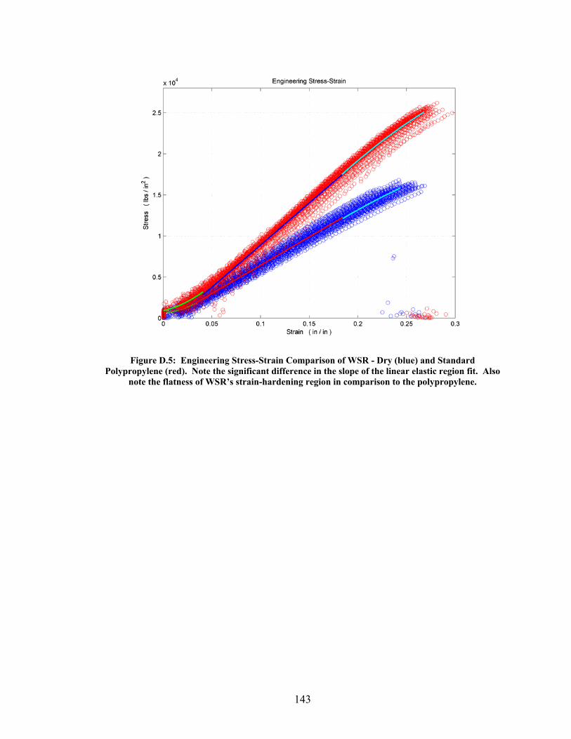
143
Figure D.5: Engineering Stress-Strain Comparison of WSR - Dry (blue) and Standard
Polypropylene (red). Note the significant difference in the slope of the linear elastic region fit. Also note the flatness of WSR’s strain-hardening region in comparison to the polypropylene.

144
APPENDIX E:
First Derivative of Stress with Respect to Time

145
Figure E.1: First Derivative of Stress for WSR-Dry. Raw data for each replicate (blue), piecewise
fits for the positive and negative sections (red), the intersection of the fits (green), and the 95% Confidence interval (black dash)
Figure E.2: First Derivative of Stress for WSR-Wet. Raw data for each replicate (blue), piecewise
fits for the positive and negative sections (red), the intersection of the fits (green), and the 95% Confidence interval (black dash).

146
Figure E.3: First derivative of stress comparison between dry (blue) and wet (red) WSR.
Figure E.4: First Derivative of Stress for Polypropylene. Raw data for each replicate (blue),
piecewise fits for the positive and negative sections (red), the intersection of the fits (green), and the 95% Confidence interval (black dash).

147
Figure E.5: First derivative of stress comparison between WSR-Dry (blue) and Standard
Polypropylene (red). Note that the WSR is much flatter as compared to the polypropylene.

148
APPENDIX F:
Second Derivative of Stress with Respect to Time

149
Figure F.1: Second derivative of stress for WSR-Dry. Raw data for each replicate (blue), curve fit of
the data (red), and 95% Confidence interval (black dash). Note the negative slope of the fit line.
Figure F.2: Second derivative of stress for WSR-Wet. Raw data for each replicate (blue), curve fit of
the data (red), and 95% Confidence interval (black dash). Note the negative slope of the fit line.

150
Figure F.3: Comparison between the dry (blue) and wet (red) WSR second derivative of stress.
Figure F.4: Second derivative of stress for polypropylene. Raw data for each replicate (blue), curve fit of the data (red), and 95% Confidence interval (black dash). Note the negative slope of the fit line.

151
Figure F.5: Comparison of the second derivative of stress between WSR-dry (blue) and standard
polypropylene (red)