CHARACTERIZATION OF TWO VERNIER TUNED DISTRIBUTED BRAGG

REFLECTOR (VT-DBR) LASERS USED IN SWEPT SOURCE OPTICAL

COHERENCE TOMOGRAPHY (SS-OCT)

A Thesis

presented to

the Faculty of California Polytechnic State University,

San Luis Obispo

In Partial Fulfillment

of the Requirements for the Degree

Master of Science in Electrical Engineering

by

Gregory M. Bergdoll

June 2015

ii

© 2015

Gregory M. Bergdoll

ALL RIGHTS RESERVED

iii

COMMITTEE MEMBERSHIP

TITLE:

AUTHOR:

DATE SUBMITTED:

COMMITTEE CHAIR:

COMMITTEE MEMBER:

COMMITTEE MEMBER:

COMMITTEE MEMBER:

Characterization of two Vernier-Tuned

Distributed Bragg Reflector (VT-DBR) Lasers

used in Swept Source Optical Coherence

Tomography (SS-OCT)

Gregory M. Bergdoll

June 2015

Dennis Derickson, Ph.D. Department Chair of Electrical Engineering

Jason Ensher, Ph.D. Engineering VP of Insight Photonic Solutions Inc. Xiaomin Jin, Ph.D. Associate Professor of Electrical Engineering Bridget Benson, Ph.D. Assistant Professor of Electrical Engineering

iv

ABSTRACT

Characterization of two Vernier-Tuned Distributed Bragg Reflector (VT-DBR)

Lasers used in Swept Source Optical Coherence Tomography (SS-OCT)

Gregory M. Bergdoll

Insight Photonic Solutions Inc. has continued to develop their patented VT-DBR laser design; these wavelength tunable lasers promise marked image-quality and acquisition time improvements in SS-OCT applications. To be well suited for SS-OCT, tunable lasers must be capable of producing a highly linear wavelength sweep across a tuning range well-matched to the medium being imaged; many different tunable lasers used in SS-OCT are compared to identify the optimal solution. This work electrically and spectrally characterizes two completely new all-semiconductor VT-DBR designs to compare, as well. The Neptune VT-DBR, an O-band laser, operates around the 1310 nm range and is a robust solution for many OCT applications. The VTL-2 is the first 1060 nm VT-DBR laser to be demonstrated. It offers improved penetration through water over earlier designs which operate at longer wavelengths (e.g. - 1550 nm and 1310 nm), making it an optimal solution for the relatively deep imaging requirements of the human eye; the non-invasive nature of OCT makes it the ideal imaging technology for ophthalmology. Each laser has five semiconductor P-N junction segments that collectively enable precise akinetic wavelength-tuning (i.e. - the tuning mechanism has no moving parts). In an SS-OCT system utilizing one of these laser packages, the segments are synchronously driven with high speed current signals that achieve the desired wavelength, power, and sweep pattern of the optical output. To validate the laser’s fast tuning response time necessary for its use in SS-OCT, a circuit model of each tuning section is created; each laser section is modeled as a diode with a significant lead inductance. The dynamic resistance, effective capacitance, and lead inductance of this model are measured as a function of bias current and the response time corresponding to each bias condition is determined. Tuning maps, spectral linewidths, and side-mode suppression ratio (SMSR) measurements important to SS-OCT performance are also collected. Measured response times vary from 700 ps to 2 ns for the Neptune and 1.2 to 2.3 ns for the VTL-2. Linewidth measurements range from 9 MHz to 124 MHz for the Neptune and 300 kHz to 2 MHz for the VTL-2. SMSR measurements greater than 38 dB and 40 dB were observed for the Neptune and VTL-2, respectively. Collectively, these results implicate the VT-DBR lasers as ideal tunable sources for use in SS-OCT applications. Keywords: semiconductor laser, vernier, Bragg-reflector, optical coherence tomography, dynamic resistance, reflectometry, spectral linewidth, and SMSR.

v

ACKNOWLEDGMENTS

Thank you Insight Photonic Solutions for developing the VT-DBR lasers

and making my thesis research possible. Dr. Jason Ensure, thank you for

supporting my thesis work and taking time to answer all my questions. Dr. Dennis

Derickson, thank you for giving me this research opportunity, guiding my

exploration, and sharing your knowledge in photonics. It has been a pleasure to

work with you all. Family, friends, and colleagues, thank you for your confidence

in me; your support has made all my academic success possible.

vi

TABLE OF CONTENTS

Page

LIST OF TABLES ............................................................................................... viii

LIST OF FIGURES ...............................................................................................ix

1. INTRODUCTION .............................................................................................. 1

Tunable Lasers ................................................................................................. 1

Vernier Tuned Distributed Bragg Reflector (VT-DBR) Lasers ........................... 2

Swept Source Optical Coherence Tomography (SS-OCT) ............................... 8

Comparable Tunable Lasers for SS-OCT ....................................................... 13

2. OBJECTIVES ................................................................................................. 15

3. ELECTRICAL CHARACTERIZATION ............................................................ 22

I-V Curves ....................................................................................................... 22

FDR and TDR Response ................................................................................ 24

Dynamic Resistance Extraction from TDR ...................................................... 25

Response Time Extraction from FDR ............................................................. 28

TDR Measurement Validation ......................................................................... 31

4. SPECTRAL CHARACTERIZATION ............................................................... 36

Tuning Maps ................................................................................................... 36

Side-Mode Suppression Ratio ........................................................................ 39

Spectral Linewidth ........................................................................................... 40

5. NEPTUNE VT-DBR LASER CHARACTERIZATION ...................................... 42

vii

6. VTL-2 VT-DBR LASER CHARACTERIZATION ............................................. 57

7. SUMMARY OF RESULTS .............................................................................. 65

8. FUTURE WORK ............................................................................................. 68

BIBLIOGRAPHY ................................................................................................. 70

APPENDICES .................................................................................................... 72

Appendix A: Butterfly Laser Package Pinout Diagram .................................... 72

Appendix B: Tabulated RLC Data for the 1310nm Neptune Laser ................. 73

Appendix C: Tabulated RLC Data for the 1060nm VTL-2 Laser ..................... 83

Appendix D: TDR Validation Measurements ................................................... 88

Appendix E: Tuning Map Matlab Functions .................................................... 89

LASERMEASUREMENT() .......................................................................... 89

TUNINGMAPPER() ..................................................................................... 96

TUNINGMAPVID() .................................................................................... 102

Appendix F: Neptune - Tuning Map Collection and Data .............................. 111

Appendix G: Neptune - SMSR Screen Captures .......................................... 112

Appendix H: Neptune - Additional OSA and Linewidth Measurements ......... 113

Appendix I: VTL-2 - SMSR Screen Captures ................................................ 116

Appendix J: VTL-2 - Linewidth Measurement Screen Captures ................... 117

Appendix K: TDR, FDR, and RLC Data of Neptune Laser ............................ 120

Appendix L: TDR, FDR, and RLC Data of VTL-2 Laser ................................ 121

Appendix M: Photograph of Automated Tuning Map Collection .................... 122

Appendix N: Photograph of Photonics Lab Workstation ............................... 123

viii

LIST OF TABLES

Table Page

1. Comparison of performance parameters among various swept source lasers used in OCT. ...................................................................................... 13

2. SMSR measurements of the Neptune laser. Gain and SOA sections are biased at 100 mA. Phase section is shorted. .......................................... 53

3. Neptune laser linewidth measurements. Gain and SOA sections are biased at 100 mA. The phase section is shorted. .......................................... 55

4. Neptune laser linewidth measurements. Gain and SOA sections are biased at 100 mA. The phase and FM sections are shorted. ........................ 56

5. Neptune laser linewidth measurements. Gain and SOA sections are biased at 100 mA. The phase and BM sections are shorted. ........................ 56

6. SMSR measurements of the VTL-2 laser. Gain and SOA sections are biased at 100 mA. Phase section is shorted. ................................................ 63

7. VTL-2 laser linewidth measurements. Gain and SOA sections are biased at 100 mA. The phase section is shorted. .......................................... 64

8. Maximum response time for each section of the Neptune VT-DBR laser. ............................................................................................................. 65

9. Maximum response time for each section of the VTL-2 VT-DBR laser. ........ 65

ix

LIST OF FIGURES

Figure Page

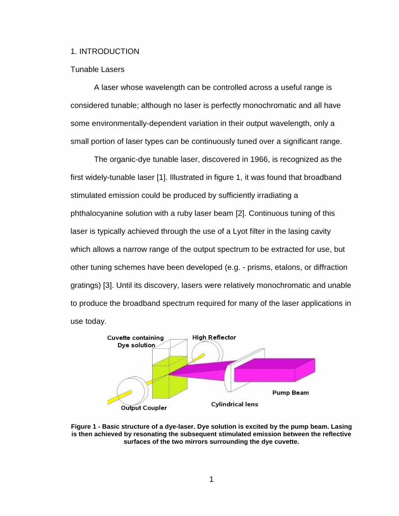
1. Basic structure of a dye-laser. Dye solution is excited by the pump beam. Lasing is then achieved by resonating the subsequent stimulated emission between the reflective surfaces of the two mirrors surrounding the dye cuvette. ........................................................................... 1

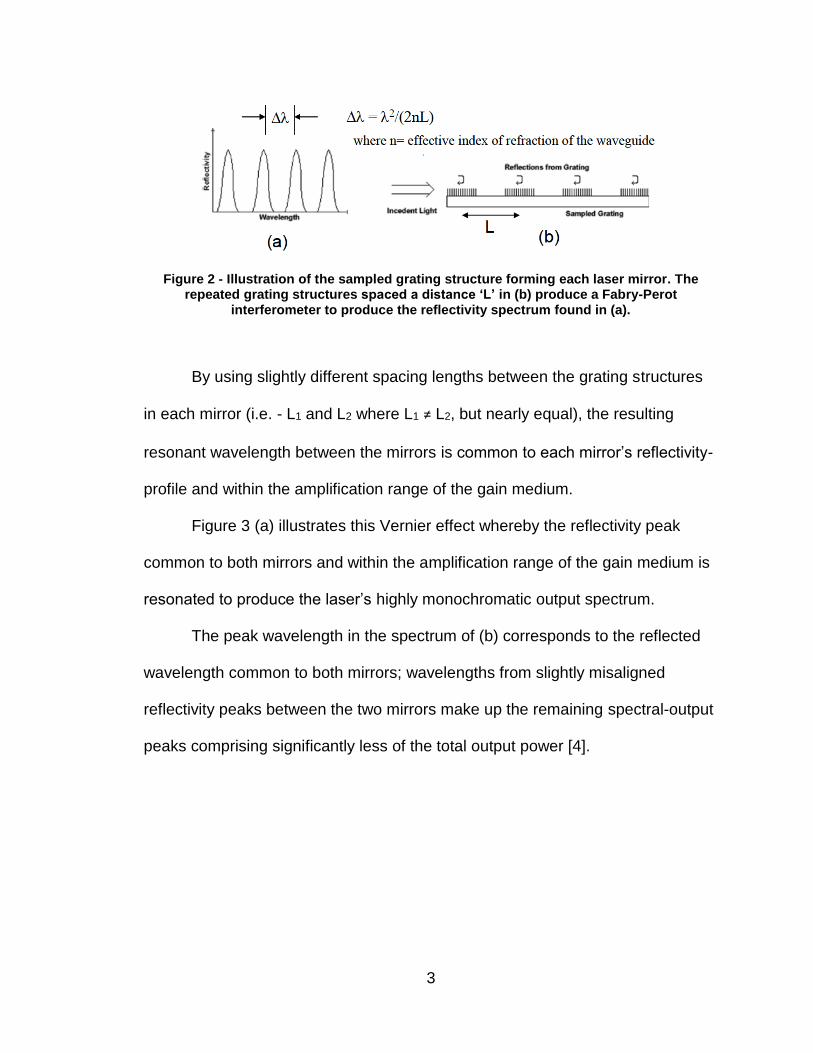
2. Illustration of the sampled grating structure forming each laser mirror. The repeated grating structures spaced a distance ‘L’ in (b) produce a Fabry-Perot interferometer to produce the reflectivity spectrum found in (a). ................................................................................................................... 3

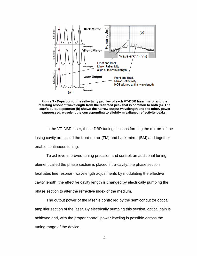
3. Depiction of the reflectivity profiles of each VT-DBR laser mirror and the resulting resonant wavelength from the reflected peak that is common to both (a). The laser’s output spectrum (b) shows the narrow output wavelength and the other, power suppressed, wavelengths corresponding to slightly misaligned reflectivity peaks. ................................... 4

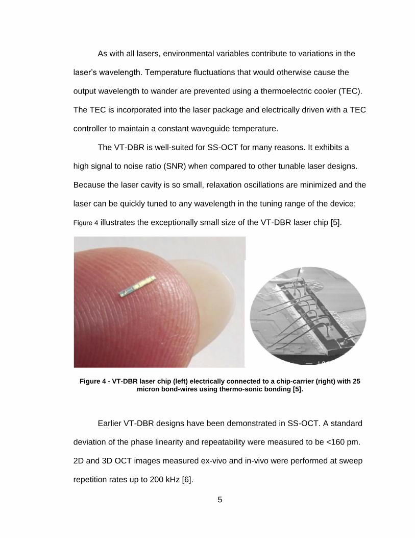
4. VT-DBR laser chip (left) electrically connected to a chip-carrier (right) with 25 micron bond-wires using thermo-sonic bonding [5]. ............................ 5

5. In vivo SS-OCT image of the epidermis using a 1550 nm VT-DBR laser. The data is rendered in 3D (a) and cut-away (b) to reveal intra-sample morphology. Single b-scan (c) and en-face view (d) of the 3D data-set demonstrates versatility of OCT imaging. .......................................... 6

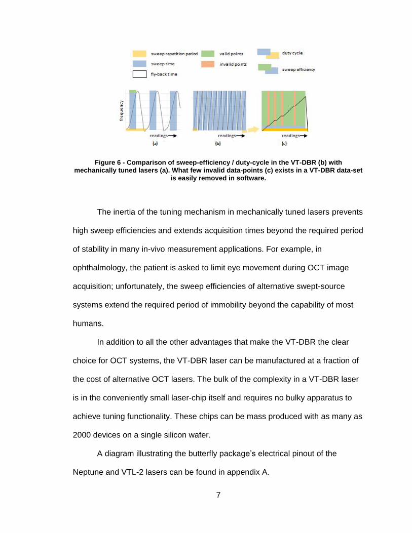
6. Comparison of sweep-efficiency / duty-cycle in the VT-DBR (b) with mechanically tuned lasers (a). What few invalid data-points (c) exists in a VT-DBR data-set is easily removed in software. .......................................... 7

7. Illustration of the output radiation properties of an incandescent lamp, LED, and laser pointer. Directional, monochromatic, and coherent light is unique to laser radiation. ............................................................................. 8

8. OCT images of the retina. A three-dimensional data-set can be processed to produce enface images (d, e, and h), b-scans (b, g), and a 3D rendering of the eye-tissue’s morphology. .............................................. 9

9. Cross-sectional (i.e. - B-scan) image of an eye using frequency-domain optical coherence tomography (FD-OCT). ........................................ 11

x

10. Graph comparing the resolution and penetration depth of non-invasive imaging technologies used in bio-medical applications. ................................ 12

11. Thorlabs SS-OCT system utilizing the MEMS-VCSEL tuning scheme. ......... 14

12. Santec SS-OCT system utilizing the polygon mirror tuning scheme. ............ 14

13. Assumed circuit model of each laser section; lead inductance, effective capacitance, and dynamic resistance are all represented by lumped components. .................................................................................................. 15

14. Internal view of the VT-DBR laser package; 25 micron bond-wires connecting the laser’s package to the chip carrier and chip carrier to the laser chip are made using thermosonic bonding. .................................... 16

15. Close-up view of the bond-wire connections between chip carrier and the laser chip in a VT-DBR laser package..................................................... 17

16. VT-DBR laser break-out board for use in the characterization of VT-DBR lasers. All key components labeled including the Butterfly package, TEC connections, 50 Ω PCB traces, and SMA port connections. .................................................................................................. 17

17. IV curve collection instrument-setup. A laser-diode controller (i.e. - LDC-3744B) is used to drive the on-chip TEC and provide the current bias to the PUT. A current-limiting resistor is used to protect the PUT from transient voltage/current spikes and provide a point to measure the PUT voltage. An HP 34401A voltmeter is used to measure the PUT voltage........................................................................................................... 22

18. Gain port voltage measurement of the Neptune laser with a 1.9 mA current bias being delivered from the laser-diode controller. An 881 mV port voltage is observed. ............................................................................... 23

19. VNA instrument configuration used to collect the TDR and FCR responses of each PUT. An LDC-3744B is used to drive the onchip TEC and deliver bias current through the "Port 1 Bias" connection on the back panel of the VNA. The VNA is first calibrated and reference plane shifted to the beginning of the package leads. The measurement reference plane is identified by the dashed red lines on the breakout board PCB. .................................................................................................... 24

20. Butterfly package break-out board designed by Desmond Talkington for experimental research of the packaged VT-DBR lasers; a 50 Ω electrical system is used to reduce source signal reflection and achieve an accurate measurement of the lumped component values in the PUT. .............................................................................................................. 25

xi

21. Example TDR response with measurement points of interest identified. The rise time (τr) and the steady state reflection coefficient (ρ) corresponding to the dynamic resistance are recorded for each bias condition. ....................................................................................................... 26

22. Typical I-V curve of a diode across the breakdown, reverse-bias, and forward-bias regions of operation. ................................................................. 27

23. Frequency domain reflectometry measurement of the Neptune laser's front-mirror section with zero current bias. .................................................... 29

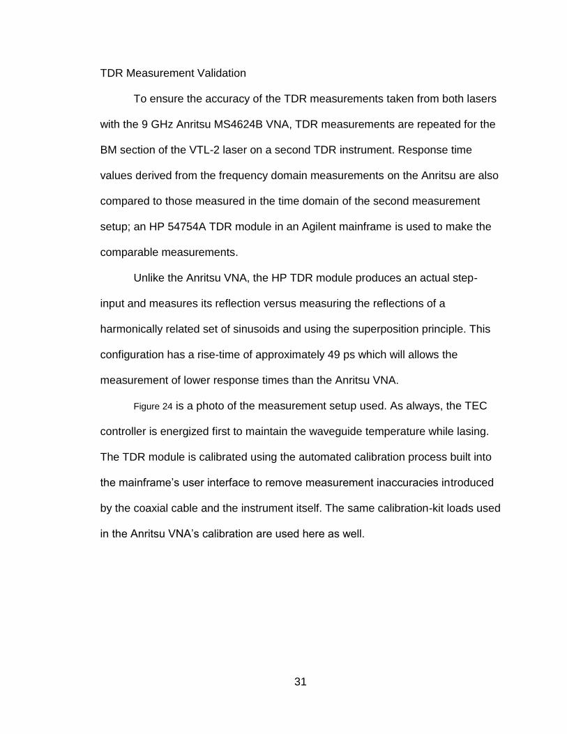
24. TDR validation instrument configuration. HP 54754A TDR module is connected to the PUT through a bias-T; the PUT is biased with the LDC current source. ...................................................................................... 32

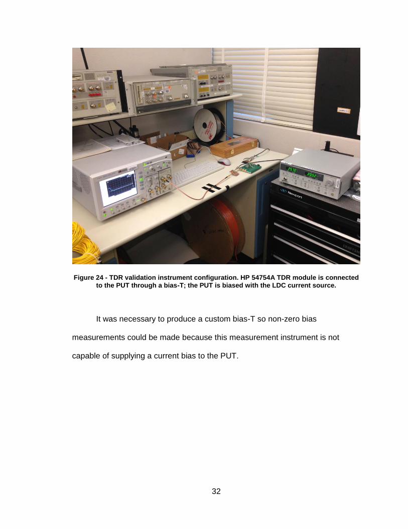
25. Custom bias-T enabling non-zero current measurements with an HP 54754A TDR module. The bias connection forms a low-pass filter to prevent TDR stimuli from reaching the bias source. The stimulus signal is transferred to the PUT via an AC coupling capacitor. ................................ 33

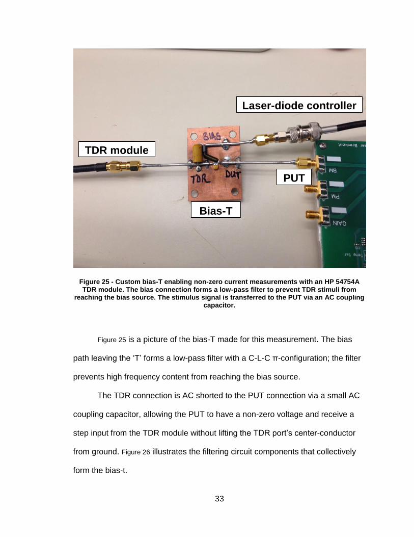
26. Bias-T circuit schematic. ............................................................................... 34

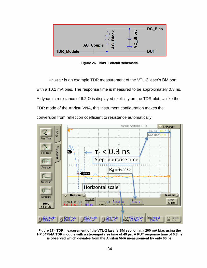
27. TDR measurement of the VTL-2 laser's BM section at a 200 mA bias using the HP 54754A TDR module with a step-input rise time of 49 ps. A PUT response time of 0.3 ns is observed which deviates from the Anritsu VNA measurement by only 60 ps. ..................................................... 34

28. Comparison of the VTL-2 laser's BM section response-times between the two collection instruments and methods. A very high correlation is observed. ...................................................................................................... 35

29. Instrument configuration used for tuning map collection. The user runs the MatLab function ‘LaserMeasurement()’ with the bias current start, stop, and step/resolution values for the FM and BM precision current sources passed in the function’s argument. .................................................. 37

30. SMSR measurement example. An SMSR of greater than 27 dB is observed between the power of the dominant mode and the most powerful side-mode. ...................................................................................... 39

31. Instrument configuration for spectral linewidth measurements. SOA and Gain sections are biased at 100 mA. FM and BM sections are manually tuned using precision current sources. The laser's output is directed using an Agilent optical switch. The signal path includes an interferometer, reverse-biased photodiode, 3 dB attenuator, and electrical spectrum analyzer (ESA). This setup facilitates the self-homodyne measurements method. ............................................................... 40

xii

32. Noise floor of Agilent CXA signal analyzer used for measuring spectral linewidth and an example FWHM linewidth measurement of the Neptune laser. ............................................................................................... 41

33. I-V curve of the Neptune VT-DBR laser's front-mirror section. ...................... 42

34. I-V curve of the Neptune VT-DBR laser's back-mirror section. ..................... 43

35. I-V curve of the Neptune VT-DBR laser's phase section. .............................. 43

36. I-V curve of the Neptune VT-DBR laser's gain section. ................................. 44

37. I-V curve of the Neptune VT-DBR laser's SOA section. ................................ 44

38. TDR measurement of the Neptune laser's FM section with a 10.1 mA current bias. .................................................................................................. 45

39. FDR measurement of the Neptune laser's FM with a 100 mA current bias. A complex impedance of 1.941 + 0.0633j is observed. ........................ 46

40. Neptune laser's response times versus bias current for each PUT. .............. 47

41. Wavelength tuning map of the Neptune laser. This data-set represents the largest tuning area measured from the Neptune laser; BM and FM are biased from 0 to 100 mA at an increment of 1 mA along each tuning axis. Wavelengths range from 1272 nm (blue) to 1309 nm (red) in a tuning range of ~37 nm. ......................................................................... 48

42. Power tuning map of the Neptune laser. Data measurement points correspond to the same points used to generate the wavelength tuning map (i.e. - identical tuning current start, stop, and step values as the wavelength tuning-map data). Measured powers at stable operating points range from 1.2-4.0 dBm. ..................................................................... 49

43. Wavelength tuning map anomaly marked with a data-cursor. The anomaly is positioned at an FM bias of 51.786 mA and a BM bias of 50.386 mA with a peak output wavelength of 1297.3 nm. ............................. 50

44. Improved image of wavelength tuning map anomaly. Tuning map span is reduced to less than 2 mA along each tuning axis and the resolution is improved to 50 µA between data-points. ................................................... 51

45. Neptune laser’s side mode suppression ratio (SMSR) measured with 100 mA bias in the Gain and SOA sections. FM, BM, and Phase sections are zero-biased for this measurement. An SMSR greater than 43 dB is observed. ........................................................................................ 52

xiii

46. Stable linewidth measurement points identifies by data-cursors on the Neptune’s wavelength tuning map. ............................................................... 54

47. Example of the Neptune laser spectrum (left) and linewidth (right). Gain and SOA biased at 100 mA, FM and BM biased at 2 mA, and phase section shorted. .................................................................................. 55

48. I-V curve of the VTL-2 VT-DBR laser's front-mirror section. .......................... 57

49. I-V curve of the VTL-2 VT-DBR laser's back-mirror section. ......................... 58

50. I-V curve of the VTL-2 VT-DBR laser's phase section. .................................. 58

51. I-V curve of the VTL-2 VT-DBR laser's gain section...................................... 59

52. I-V curve of the VTL-2 VT-DBR laser's SOA section. .................................... 59

53. TDR measurement of the VTL-2 laser's BM section with a 10.1 mA current bias. .................................................................................................. 60

54. FDR measurement of the VTL-2 laser's BM with a 90.1 mA current bias. A complex impedance of 7.769 + 0.9223j is observed. ........................ 61

55. VTL-2 laser’s side mode suppression ratio (SMSR) measured with 100 mA bias in the Gain and SOA sections. FM is biased at 40.4 mA, BM is zero biased, and the phase section is shorted. A SMSR greater than 43 dB is observed. ........................................................................................ 62

56. Example of the VTL-2 laser spectrum (left) and linewidth (right). Gain and SOA biased at 100 mA, FM and BM biased at 79 mA, and phase section shorted. ............................................................................................. 63

1

1. INTRODUCTION

Tunable Lasers

A laser whose wavelength can be controlled across a useful range is

considered tunable; although no laser is perfectly monochromatic and all have

some environmentally-dependent variation in their output wavelength, only a

small portion of laser types can be continuously tuned over a significant range.

The organic-dye tunable laser, discovered in 1966, is recognized as the

first widely-tunable laser [1]. Illustrated in figure 1, it was found that broadband

stimulated emission could be produced by sufficiently irradiating a

phthalocyanine solution with a ruby laser beam [2]. Continuous tuning of this

laser is typically achieved through the use of a Lyot filter in the lasing cavity

which allows a narrow range of the output spectrum to be extracted for use, but

other tuning schemes have been developed (e.g. - prisms, etalons, or diffraction

gratings) [3]. Until its discovery, lasers were relatively monochromatic and unable

to produce the broadband spectrum required for many of the laser applications in

use today.

Figure 1 - Basic structure of a dye-laser. Dye solution is excited by the pump beam. Lasing is then achieved by resonating the subsequent stimulated emission between the reflective

surfaces of the two mirrors surrounding the dye cuvette.

2

Vernier Tuned Distributed Bragg Reflector (VT-DBR) Lasers

VT-DBR lasers are a type of semiconductor tunable laser that achieve

wavelength tuning by selecting the lasing cavity’s oscillatory wavelength with two

sampled grating distributed Bragg-reflector (SG-DBR) mirrors on either end of

the cavity. An SG-DBR mirror is comprised of a set of evenly spaced distributed-

Bragg reflectors (DBR); together they perform as a Fabry-Perot resonator,

rejecting the transmission of a harmonically related set of wavelengths

determined by the length of separation between its DBR structures; the rejected

light is resonated in an electrically pumped active medium called the gain

section. In this region of the cavity, a single mode commonly reflected by both

DBR mirrors experiences significant amplification.

The distance light must travel between each mirror’s repeated grating

structure is controlled by pumping the semiconductor material it is comprised of

with electric current; this changes the refractive index of the material which alters

the reflective angle of incidence, changing the light-path distance between

structures. Subsequently, the rejected wavelength common to both mirrors is

oscillated through the gain medium where coherent amplification is achieved.

Figure 2 illustrates the DBR structure of each mirror. It can be seen that each

sampled grating mirror reflects a harmonically related set of wavelengths

dependent on the incident light’s wavelength, the effective index of refraction ‘n’,

and the distance between the repeated grating structures ‘L’ [4].

3

Figure 2 - Illustration of the sampled grating structure forming each laser mirror. The repeated grating structures spaced a distance ‘L’ in (b) produce a Fabry-Perot

interferometer to produce the reflectivity spectrum found in (a).

By using slightly different spacing lengths between the grating structures

in each mirror (i.e. - L1 and L2 where L1 ≠ L2, but nearly equal), the resulting

resonant wavelength between the mirrors is common to each mirror’s reflectivity-

profile and within the amplification range of the gain medium.

Figure 3 (a) illustrates this Vernier effect whereby the reflectivity peak

common to both mirrors and within the amplification range of the gain medium is

resonated to produce the laser’s highly monochromatic output spectrum.

The peak wavelength in the spectrum of (b) corresponds to the reflected

wavelength common to both mirrors; wavelengths from slightly misaligned

reflectivity peaks between the two mirrors make up the remaining spectral-output

peaks comprising significantly less of the total output power [4].

4

Figure 3 - Depiction of the reflectivity profiles of each VT-DBR laser mirror and the resulting resonant wavelength from the reflected peak that is common to both (a). The laser’s output spectrum (b) shows the narrow output wavelength and the other, power

suppressed, wavelengths corresponding to slightly misaligned reflectivity peaks.

In the VT-DBR laser, these DBR tuning sections forming the mirrors of the

lasing cavity are called the front-mirror (FM) and back-mirror (BM) and together

enable continuous tuning.

To achieve improved tuning precision and control, an additional tuning

element called the phase section is placed intra-cavity; the phase section

facilitates fine resonant wavelength adjustments by modulating the effective

cavity length; the effective cavity length is changed by electrically pumping the

phase section to alter the refractive index of the medium.

The output power of the laser is controlled by the semiconductor optical

amplifier section of the laser. By electrically pumping this section, optical gain is

achieved and, with the proper control, power leveling is possible across the

tuning range of the device.

5

As with all lasers, environmental variables contribute to variations in the

laser’s wavelength. Temperature fluctuations that would otherwise cause the

output wavelength to wander are prevented using a thermoelectric cooler (TEC).

The TEC is incorporated into the laser package and electrically driven with a TEC

controller to maintain a constant waveguide temperature.

The VT-DBR is well-suited for SS-OCT for many reasons. It exhibits a

high signal to noise ratio (SNR) when compared to other tunable laser designs.

Because the laser cavity is so small, relaxation oscillations are minimized and the

laser can be quickly tuned to any wavelength in the tuning range of the device;

Figure 4 illustrates the exceptionally small size of the VT-DBR laser chip [5].

Figure 4 - VT-DBR laser chip (left) electrically connected to a chip-carrier (right) with 25 micron bond-wires using thermo-sonic bonding [5].

Earlier VT-DBR designs have been demonstrated in SS-OCT. A standard

deviation of the phase linearity and repeatability were measured to be <160 pm.

2D and 3D OCT images measured ex-vivo and in-vivo were performed at sweep

repetition rates up to 200 kHz [6].

6

Figure 5 depicts an example 3D image from a VT-DBR laser. The 1.5 GB

data-set associated with this image was acquired in ~2.4 seconds. This high rate

of data-acquisition makes the VT-DBR laser the most practical solution for in vivo

OCT imaging.

Figure 5 - In vivo SS-OCT image of the epidermis using a 1550 nm VT-DBR laser. The data is rendered in 3D (a) and cut-away (b) to reveal intra-sample morphology. Single b-scan (c)

and en-face view (d) of the 3D data-set demonstrates versatility of OCT imaging.

The fast data acquisition and superior imaging-quality of VT-DBR lasers

are made possible by the sweep efficiency and data rejection illustrated in Figure

6. The few non-linear regions of the OCT sweep are removed from the data-set

and the resulting image resolution is improved.

7

Figure 6 - Comparison of sweep-efficiency / duty-cycle in the VT-DBR (b) with mechanically tuned lasers (a). What few invalid data-points (c) exists in a VT-DBR data-set

is easily removed in software.

The inertia of the tuning mechanism in mechanically tuned lasers prevents

high sweep efficiencies and extends acquisition times beyond the required period

of stability in many in-vivo measurement applications. For example, in

ophthalmology, the patient is asked to limit eye movement during OCT image

acquisition; unfortunately, the sweep efficiencies of alternative swept-source

systems extend the required period of immobility beyond the capability of most

humans.

In addition to all the other advantages that make the VT-DBR the clear

choice for OCT systems, the VT-DBR laser can be manufactured at a fraction of

the cost of alternative OCT lasers. The bulk of the complexity in a VT-DBR laser

is in the conveniently small laser-chip itself and requires no bulky apparatus to

achieve tuning functionality. These chips can be mass produced with as many as

2000 devices on a single silicon wafer.

A diagram illustrating the butterfly package’s electrical pinout of the

Neptune and VTL-2 lasers can be found in appendix A.

8

Swept Source Optical Coherence Tomography (SS-OCT)

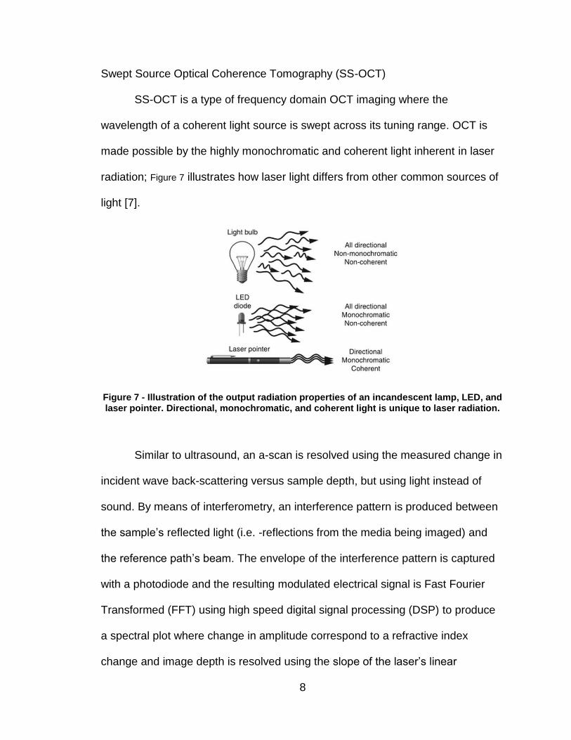
SS-OCT is a type of frequency domain OCT imaging where the

wavelength of a coherent light source is swept across its tuning range. OCT is

made possible by the highly monochromatic and coherent light inherent in laser

radiation; Figure 7 illustrates how laser light differs from other common sources of

light [7].

Figure 7 - Illustration of the output radiation properties of an incandescent lamp, LED, and laser pointer. Directional, monochromatic, and coherent light is unique to laser radiation.

Similar to ultrasound, an a-scan is resolved using the measured change in

incident wave back-scattering versus sample depth, but using light instead of

sound. By means of interferometry, an interference pattern is produced between

the sample’s reflected light (i.e. -reflections from the media being imaged) and

the reference path’s beam. The envelope of the interference pattern is captured

with a photodiode and the resulting modulated electrical signal is Fast Fourier

Transformed (FFT) using high speed digital signal processing (DSP) to produce

a spectral plot where change in amplitude correspond to a refractive index

change and image depth is resolved using the slope of the laser’s linear

9

frequency sweep (i.e. - relative sample depth is correlated to a frequency

difference in the FFT output).

Adjacent a-scans can be captured and concatenated in software to form a

b-scan (i.e. - a cross-sectional slice of the medium being imaged); likewise,

adjacent b-scans may be collected and appended together in software to render

a 3D depiction of the light-scattering media being imaged. Figure 8 illustrates

different rendering techniques used to study the morphology an eye’s retinal

tissue [8].

Figure 8 - OCT images of the retina. A three-dimensional data-set can be processed to produce enface images (d, e, and h), b-scans (b, g), and a 3D rendering of the eye-tissue’s

morphology.

10

In contrast to frequency domain OCT, time domain OCT uses a

broadband source (e.g. – a super-luminescent diode) to illuminate the sample

with its entire spectral output at once. The interference pattern at varied sample

depths is measured by longitudinally modulating the interferometer’s mirror

position in the reference-path. As with mechanically tuned laser’s, the

requirement of movement in the measurement device limits its performance in

OCT application. The finite inertia of the mirror limits the speed at which it can be

modulated and results in relatively long image acquisition times in time-domain

OCT schemes.

SS-OCT has been identified as the future of OCT because it offers better

resolution with greatly reduced acquisition speeds, due to the superior signal to

noise ratio (SNR) and high sweep repetition rates inherent to the VT-DBR laser.

According to Professor Paulo Stanga, a consultant ophthalmologist for the

Manchester Royal Eye Hospital, SS-OCT enables faster scanning speeds,

increased penetration depth, and improved image resolution over other OCT

measurement structures. In an interview, Dr. Stanga states that it will be

important for ophthalmologists to move to swept source OCT systems because it

allows for superior imaging of the vitreous, a location of the eye hard to image

with other OCT technologies; additionally, most of the modern treatments for

vision problems are administered by intro-vitreous injections in the vitreous

region; so, it is imperative for doctors to have a clear image of this structure when

determining the correct course of therapy [9].

11

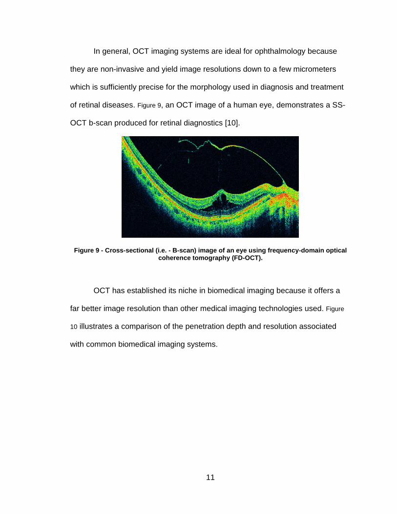
In general, OCT imaging systems are ideal for ophthalmology because

they are non-invasive and yield image resolutions down to a few micrometers

which is sufficiently precise for the morphology used in diagnosis and treatment

of retinal diseases. Figure 9, an OCT image of a human eye, demonstrates a SS-

OCT b-scan produced for retinal diagnostics [10].

Figure 9 - Cross-sectional (i.e. - B-scan) image of an eye using frequency-domain optical coherence tomography (FD-OCT).

OCT has established its niche in biomedical imaging because it offers a

far better image resolution than other medical imaging technologies used. Figure

10 illustrates a comparison of the penetration depth and resolution associated

with common biomedical imaging systems.

12

Figure 10 - Graph comparing the resolution and penetration depth of non-invasive imaging technologies used in bio-medical applications.

Despite its limited penetration depth of only a few millimeters, OCT offers

the best in-vivo imaging resolution available. A few examples from a fast-growing

list of OCT imaging applications include: dentistry, cardiovascular flow dynamics,

nondestructive testing, material thickness, and pharmaceuticals.

13

Comparable Tunable Lasers for SS-OCT

The following table shows a comparison between the current swept-

source solutions used in SS-OCT. The sweep-speed, sweep linearity, sweep

flexibility, duty cycle, tuning range, coherence length, and side-mode suppression

ratio (SMSR) of each are listed.

Table 1 - Comparison of performance parameters among various swept source lasers used in OCT.

Performance Parameter

VT-DBR Polygon MEMS-VCSEL Desirable

Sweep speed 0-200+ kHz 3-50 kHz 100/200 kHz 200+ kHz

Duty cycle >98% ~91% <70% 100%

Sweep linearity

Standard deviations < 160

pm measured

Inherently non-linear (needs wavelength reference)

Inherently non-linear (needs wavelength reference)

Perfectly linear

Sweep flexibility

Any sweep pattern possible with

akinetic-tuning Linear only Linear only

Novel sweep

patterns for

complex sensing schemes

Tuning range

30-50 nm per laser, >170

possible with output

concatenation

20-170 nm 100+ nm 50+

Coherence length

20-1000 mm 3-30 mm 11-100 mm >100 mm

SMSR 30-40 dBm ~30 dBm 40-55 dBm >25 dBm

The VT-DBR specifications are based on previous demonstrations of this

swept source technology [6] [5]. The performance specifications of the polygon

tuned source are collected from a Santec SS-OCT system and two other designs

characterized at Cal Tech University [11] [12]. The performance parameters of

the micro-electromechanical mirror system (MEMS) vertical cavity surface

14

emitting laser (VCSEL) correspond to information from Santec and Thorlabs SS-

OCT products [13] [14]. Desirable performance attributes are listed in the right

column; these values resemble the performance limits that must be met to

produce an OCT image at resolutions ranging from 3 - 20 μm.

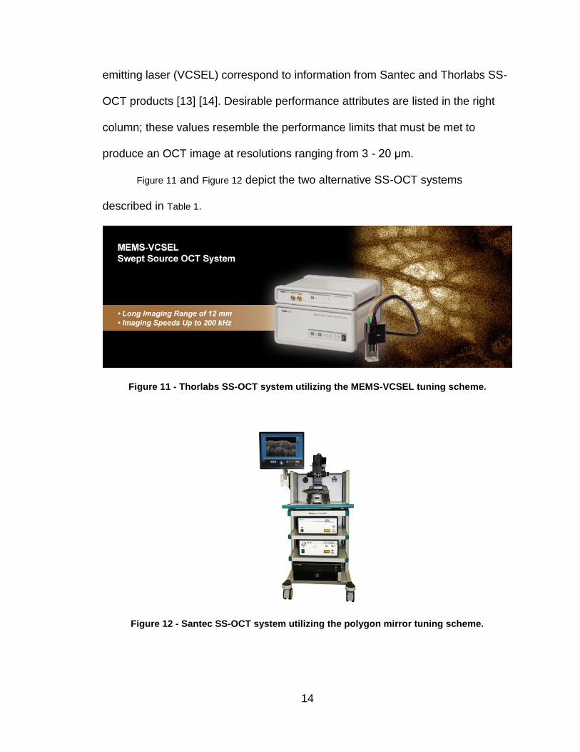
Figure 11 and Figure 12 depict the two alternative SS-OCT systems

described in Table 1.

Figure 11 - Thorlabs SS-OCT system utilizing the MEMS-VCSEL tuning scheme.

Figure 12 - Santec SS-OCT system utilizing the polygon mirror tuning scheme.

15

2. OBJECTIVES

The purpose of this work is to experimentally measure and characterize

two VT-DBR lasers to validate their usability in SS-OCT in comparison to the

alternative solutions listed in Table 1. The measured characteristics of each aid in

the development of future designs and help facilitate application-specific

performance prediction through the use of circuit modeling.

We understand that a potential limitation of the VT-DBR is the electrical

response time of each tuning section. This work seeks to quantify that delay, as it

relates directly to the optical tuning speed of the laser. The delay in a laser’s

optical response that is proportional to cavity length is minimized in the VT-DBR

due to its relatively micro size.

Each section of the VT-DBR is a semiconductor diode and the response of

each diode dictates the resulting optical response. The responses of each device

are measured to estimate optical tuning speeds.

Figure 13 is the assumed circuit model for each section of the laser where

the lead inductance, dynamic resistance, and effective capacitance are simplified

into lumped components.

Figure 13 - Assumed circuit model of each laser section; lead inductance, effective capacitance, and dynamic resistance are all represented by lumped components.

16

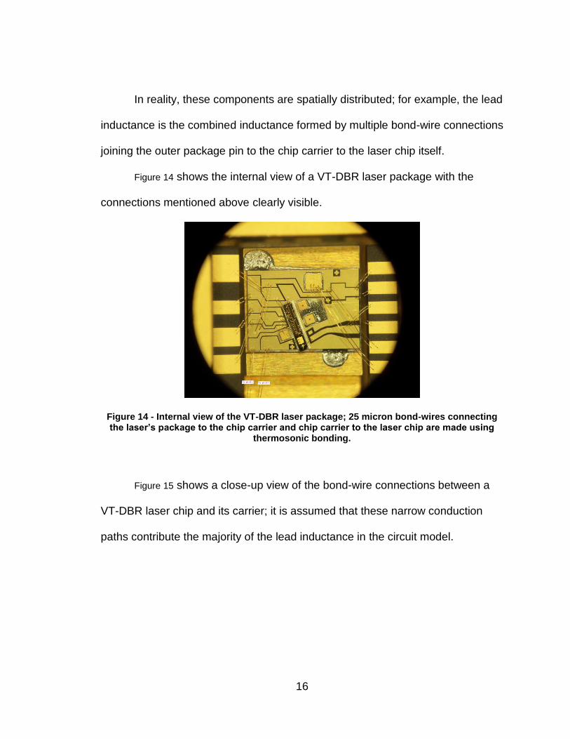
In reality, these components are spatially distributed; for example, the lead

inductance is the combined inductance formed by multiple bond-wire connections

joining the outer package pin to the chip carrier to the laser chip itself.

Figure 14 shows the internal view of a VT-DBR laser package with the

connections mentioned above clearly visible.

Figure 14 - Internal view of the VT-DBR laser package; 25 micron bond-wires connecting the laser’s package to the chip carrier and chip carrier to the laser chip are made using

thermosonic bonding.

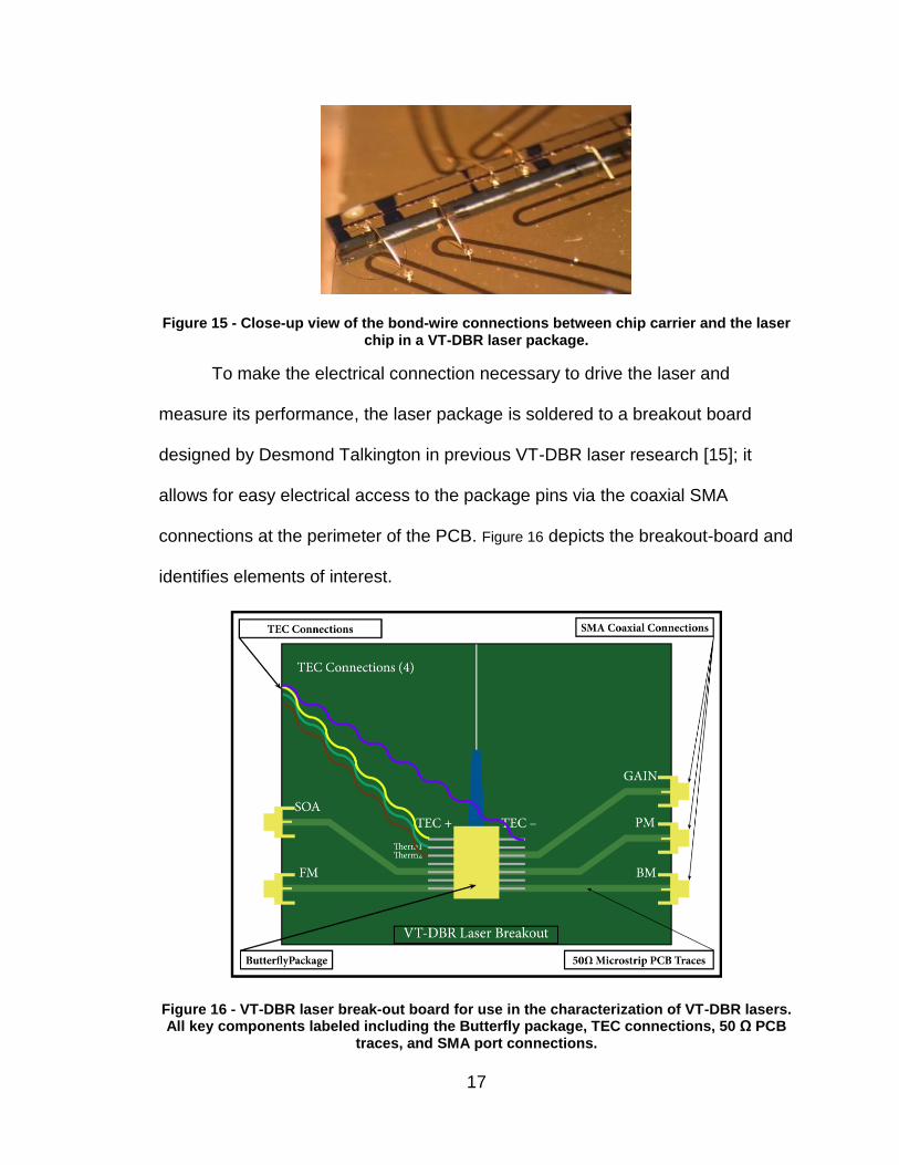
Figure 15 shows a close-up view of the bond-wire connections between a

VT-DBR laser chip and its carrier; it is assumed that these narrow conduction

paths contribute the majority of the lead inductance in the circuit model.

17

Figure 15 - Close-up view of the bond-wire connections between chip carrier and the laser chip in a VT-DBR laser package.

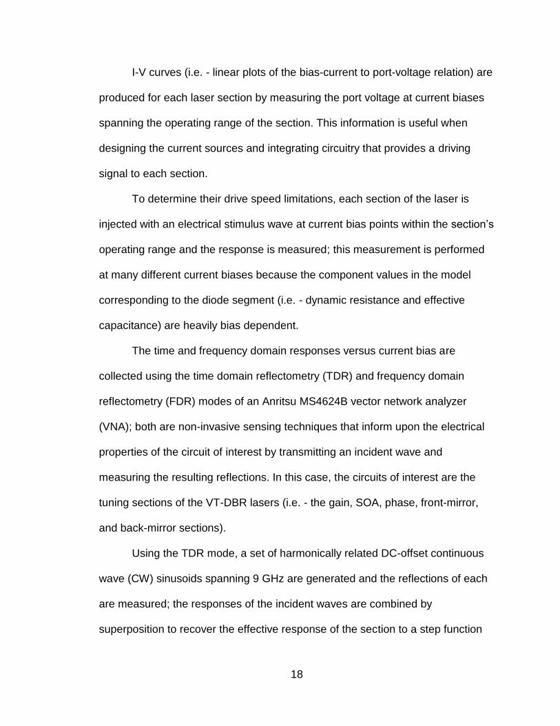
To make the electrical connection necessary to drive the laser and

measure its performance, the laser package is soldered to a breakout board

designed by Desmond Talkington in previous VT-DBR laser research [15]; it

allows for easy electrical access to the package pins via the coaxial SMA

connections at the perimeter of the PCB. Figure 16 depicts the breakout-board and

identifies elements of interest.

Figure 16 - VT-DBR laser break-out board for use in the characterization of VT-DBR lasers. All key components labeled including the Butterfly package, TEC connections, 50 Ω PCB

traces, and SMA port connections.

18

I-V curves (i.e. - linear plots of the bias-current to port-voltage relation) are

produced for each laser section by measuring the port voltage at current biases

spanning the operating range of the section. This information is useful when

designing the current sources and integrating circuitry that provides a driving

signal to each section.

To determine their drive speed limitations, each section of the laser is

injected with an electrical stimulus wave at current bias points within the section’s

operating range and the response is measured; this measurement is performed

at many different current biases because the component values in the model

corresponding to the diode segment (i.e. - dynamic resistance and effective

capacitance) are heavily bias dependent.

The time and frequency domain responses versus current bias are

collected using the time domain reflectometry (TDR) and frequency domain

reflectometry (FDR) modes of an Anritsu MS4624B vector network analyzer

(VNA); both are non-invasive sensing techniques that inform upon the electrical

properties of the circuit of interest by transmitting an incident wave and

measuring the resulting reflections. In this case, the circuits of interest are the

tuning sections of the VT-DBR lasers (i.e. - the gain, SOA, phase, front-mirror,

and back-mirror sections).

Using the TDR mode, a set of harmonically related DC-offset continuous

wave (CW) sinusoids spanning 9 GHz are generated and the reflections of each

are measured; the responses of the incident waves are combined by

superposition to recover the effective response of the section to a step function

19

with a rise time of less than 112 ps. This series of signals is generated by the

VNA and transmitted to the laser port under test (PUT) via a 50 Ω SMA coaxial

cable. The dynamic resistance corresponding to the initial DC offset bias is

determined by measuring the reflection coefficient, rho (ρ), in the TDR plot’s

steady-state response.

Using the FDR mode, the complex impedance of each laser section, from

package pin to ground, is measured as a function of current bias (i.e. - the DC

offset). The VNA generates a smith chart impedance locus by measuring the

reflections of a swept sinusoidal stimulus signal and generating a continuous plot

of impedance versus stimulus frequency. The impedance corresponding to an

input stimulus of 10 MHz is recorded, as this represents the worst case scenario

and upper bound of section drive signals that might be used.

For each section, the lead inductance is estimated using the largest

positive-reactance in the series of impedance measurements made for that PUT.

Effective capacitance is estimated by subtracting the inductive reactance from

the total measured reactance, calculating the susceptance (B), and solving for

the effective capacitance that would produce a susceptance of B in the circuit

model.

In addition to fast sweep speeds and flexibility. The optical output of the

laser requires narrow linewidth, wide spectral tuning, and good SMSR

characteristics to perform well in SS-OCT applications. Table 1 lists the desired

spectral characteristics necessary for SS-OCT. The spectral characteristics

presented in this work include high-resolution tuning maps produced using

20

computer automation, SMSR measurements, and spectral linewidths at tuning

section bias points of interest.

MatLab, a computer program, is used to achieve the automated

wavelength tuning and measurement; the function “LaserMeasurement()”

presented in appendix E commands two precision current sources connected to

the FM and BM tuning ports of the VT-DBR break-out board through a series of

bias conditions. The range and resolution of the bias currents in the data-set are

defined by the user in the argument of the function. The output of the laser is

measured with an optical spectrum analyzer (OSA) to determine the wavelength

and peak power of the dominant signal.

The bias condition, wavelength, and power measurement data are then

used by the function “TuningMapper()” to generate power and wavelength tuning-

maps useful for identifying the tuning path and operating points of interest.

A novel way of presenting the tuning-map in a video format is also

presented; using the “TuningMapVid()” function, a video showing a birds-eye

view of the tuning map structure is generated. This tool further aids the

visualization of the tuning map structure and offers a quick way to explore the

tunable spectrum of the laser.

Aided by the tuning-maps, linewidth measurement points are selected by

identifying operating points with stable single mode operation. Full width half

maximum (FWHM) linewidth measurements are made using the self-homodyne

method. This measurement technique makes use of an interferometer, DC-

21

biased photodiode, and spectrum analyzer to make accurate spectral linewidth

measurements.

The SMSR is also collected at bias points of interest to estimate the signal

to noise ratio (SNR) of the laser.

Before lasing, the TEC is always energized to prevent damage to the

device from overheating. A constant waveguide temperature of 25 +/- 0.05

degrees is always maintained when lasing to eliminate performance variations

due to temperature fluctuations.

22

3. ELECTRICAL CHARACTERIZATION

I-V Curves

The following figure depicts the test configuration used to collect the I-V

curves associated with each laser segment. An LDC-3744B laser diode controller

(LDC) is used to fix the waveguide temperature and supply a precise current bias

to the PUT. A 34401A Agilent voltmeter is used to measure the resulting voltage

that develops at the PUT, given a current bias from the LDC.

Figure 17 - IV curve collection instrument-setup. A laser-diode controller (i.e. - LDC-3744B) is used to drive the on-chip TEC and provide the current bias to the PUT. A current-limiting

resistor is used to protect the PUT from transient voltage/current spikes and provide a point to measure the PUT voltage. An HP 34401A voltmeter is used to measure the PUT

voltage.

23

The current to voltage relation is measured by stepping the input current

of the PUT through incremental bias points within its operating range and the

resulting port voltage is recorded; all bias and subsequent PUT voltages are

tabulated in an excel document.

The current-limiting resistor protects each section from transient current

spikes that might otherwise damage the device; this resistor also gives access to

the coaxial center-conductor so the port voltage can be easily measured.

The measured I-V curves inform upon the current and voltage range

requirements necessary to drive each laser section. A key element in the

assumed circuit model of each section, the dynamic resistance, is also embodied

by the inverse slop of a line tangent to the curve at a particular voltage.

All other break-out board ports are short-circuited to prevent deviations in

the measurement results due to electrical interference between the adjacent

signal paths.

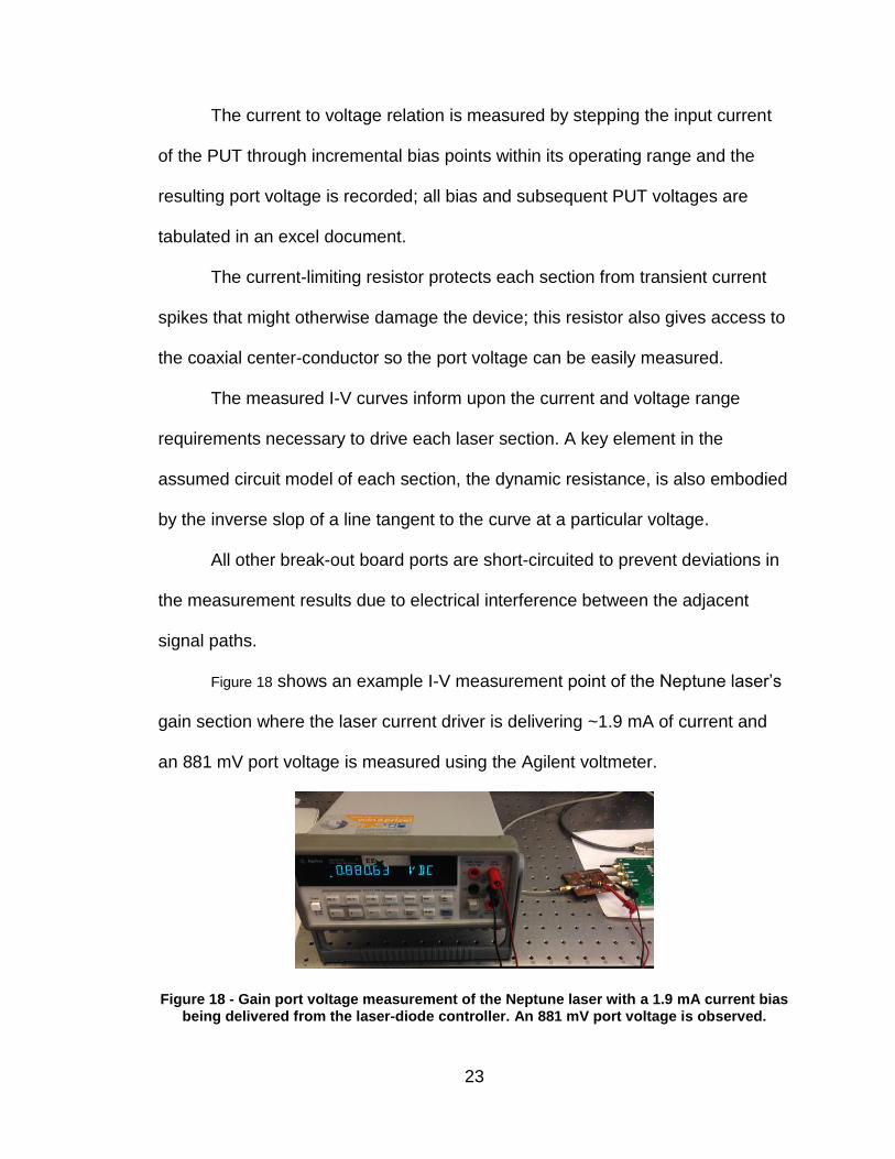
Figure 18 shows an example I-V measurement point of the Neptune laser’s

gain section where the laser current driver is delivering ~1.9 mA of current and

an 881 mV port voltage is measured using the Agilent voltmeter.

Figure 18 - Gain port voltage measurement of the Neptune laser with a 1.9 mA current bias being delivered from the laser-diode controller. An 881 mV port voltage is observed.

24

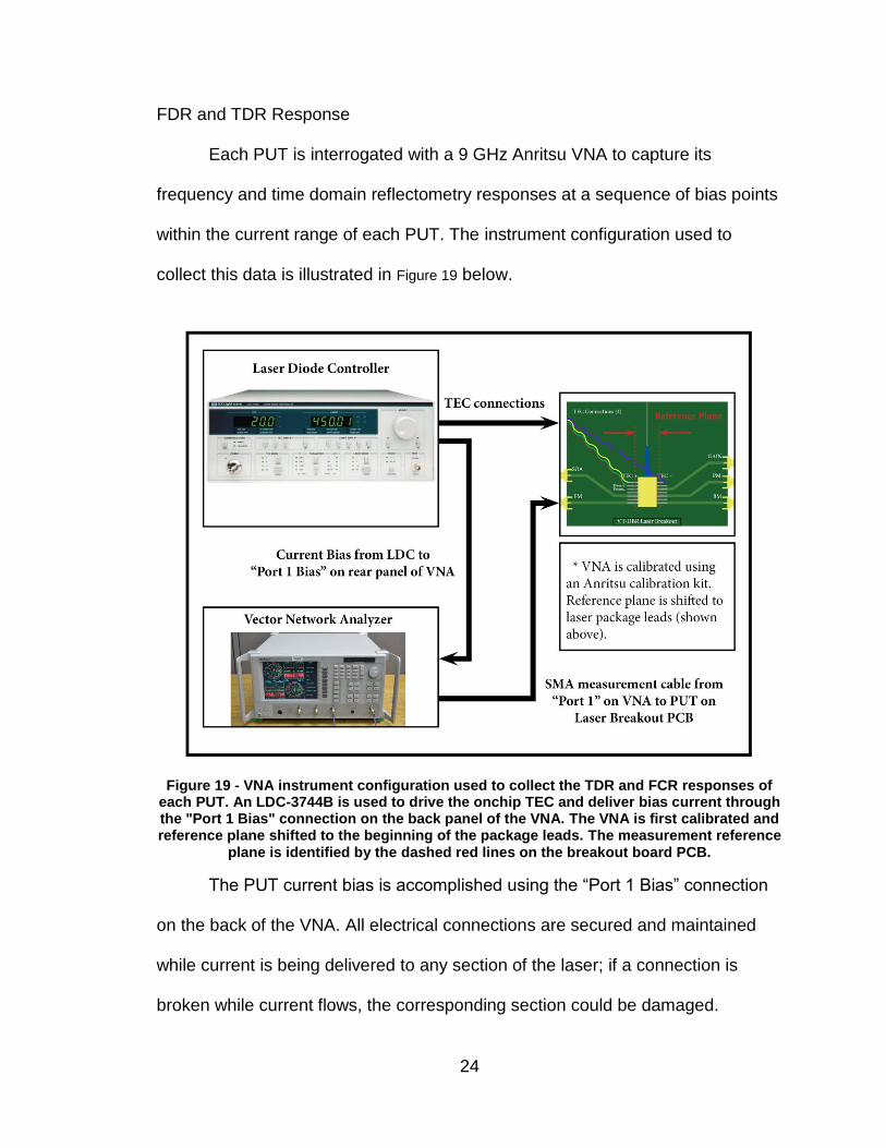
FDR and TDR Response

Each PUT is interrogated with a 9 GHz Anritsu VNA to capture its

frequency and time domain reflectometry responses at a sequence of bias points

within the current range of each PUT. The instrument configuration used to

collect this data is illustrated in Figure 19 below.

Figure 19 - VNA instrument configuration used to collect the TDR and FCR responses of each PUT. An LDC-3744B is used to drive the onchip TEC and deliver bias current through the "Port 1 Bias" connection on the back panel of the VNA. The VNA is first calibrated and reference plane shifted to the beginning of the package leads. The measurement reference

plane is identified by the dashed red lines on the breakout board PCB.

The PUT current bias is accomplished using the “Port 1 Bias” connection

on the back of the VNA. All electrical connections are secured and maintained

while current is being delivered to any section of the laser; if a connection is

broken while current flows, the corresponding section could be damaged.

25

Dynamic Resistance Extraction from TDR

The Dynamic resistance is measured by analyzing the steady-state

response of the TDR measurement. The VNA is first calibrated to remove

measurement error introduced by the measurement system itself. Once

calibrated, the VNA’s reference plane is shifted to the input of the PUT; the

spatial reference shift and windowing features of the VNA allow for the accurate

measurement of the S11 scattering parameter, limited only by its 112 ps rise-time.

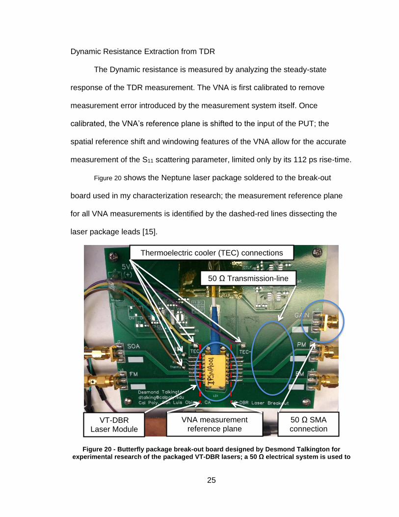
Figure 20 shows the Neptune laser package soldered to the break-out

board used in my characterization research; the measurement reference plane

for all VNA measurements is identified by the dashed-red lines dissecting the

laser package leads [15].

Figure 20 - Butterfly package break-out board designed by Desmond Talkington for experimental research of the packaged VT-DBR lasers; a 50 Ω electrical system is used to

Thermoelectric cooler (TEC) connections

VT-DBR Laser Module

50 Ω Transmission-line

50 Ω SMA connection

VNA measurement reference plane

26

reduce source signal reflection and achieve an accurate measurement of the lumped component values in the PUT.

Next, the TDR response of each PUT is measured at a sequence of bias

points and the dynamic resistance is calculated at each using the steady-state

reflected voltage waveform. Additionally, the response time (τr) can be visually

estimated by measuring the elapsed time between the incident signal’s arrival to

the reference plane and the 63.2% point of the section’s voltage transition.

The VNA is put into TDR mode and the step input response plot is

displayed. Figure 21 illustrates the measurement points of interest on the response

plot, including the response time and reflection coefficient (ρ).

Figure 21 - Example TDR response with measurement points of interest identified. The rise time (τr) and the steady state reflection coefficient (ρ) corresponding to the dynamic

resistance are recorded for each bias condition.

τr

63% of Vmax

ρ

27

Equation (1) relates the reflection coefficient measured at Vmax to the

dynamic resistance of the PUT at the particular bias. 𝑍𝑜 represents the 50 Ω

characteristic impedance of the transmission lines used to connect the VNA to

the laser’s package leads. Every TDR measurement for the Neptune and VTL-2

lasers can be found in the corresponding ‘.zip’ files in appendix K and L,

respectively.

(1)

Figure 22 illustrates the relation between the dynamic resistance and an I-V

curve of a typical diode. At a particular bias point, the dynamic resistance of a

diode is defined by the inverse-slope of the tangent line at that point. From the

illustration, it is clear that this dynamic resistance of a diode changes dramatically

across its operating range.

Figure 22 - Typical I-V curve of a diode across the breakdown, reverse-bias, and forward-bias regions of operation.

𝑹𝒅 = 𝒁𝒐

(𝟏 + 𝛒)

(𝟏 − 𝛒)

𝛥𝑖 @ V= Vd

𝑹𝒅 = 𝛥𝑣

𝛥𝑖

𝛥𝑣

28

Response Time Extraction from FDR

The complex impedance of each PUT is also measured at the same bias

points used for the TDR measurements. The VNA mode is changed to display

the FDR response in the form of a smith chart. A marker is placed on the

impedance locus point corresponding to a 10 MHz stimulus.

As in the TDR measurements, the plot data is taken at each bias point and

the complex impedance is recorded in an excel spreadsheet. This data is then

used to estimate the fixed lead-inductance and bias dependent effective-

capacitance.

Figure 23 identifies the pertinent information in an example FDR

measurement. As with the TDR data, every FDR measurement for the Neptune

and VTL-2 lasers can be found in the corresponding ‘.zip’ files in appendix K and

L, respectively.

The largest reactance measured for each PUT is rounded up to the

nearest tenth of an ohm to account for the finite reactance contribution of the

effective capacitance. The inductive reactance is then used to estimate the fixed

lead inductance using equation (2).

(2) 𝑳𝒍𝒆𝒂𝒅 =𝑿𝑳

𝟐𝝅𝒇

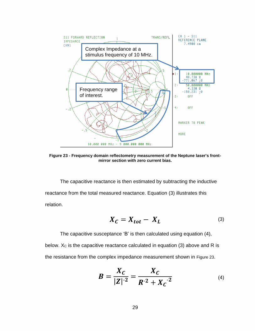
29

Figure 23 - Frequency domain reflectometry measurement of the Neptune laser's front-mirror section with zero current bias.

The capacitive reactance is then estimated by subtracting the inductive

reactance from the total measured reactance. Equation (3) illustrates this

relation.

(3)

The capacitive susceptance ‘B’ is then calculated using equation (4),

below. XC is the capacitive reactance calculated in equation (3) above and R is

the resistance from the complex impedance measurement shown in Figure 23.

(4)

𝑿𝑪 = 𝑿𝒕𝒐𝒕 − 𝑿𝑳

𝑩 =𝑿𝑪

|𝒁|-𝟐=

𝑿𝑪

𝑹-𝟐 + 𝑿𝑪-𝟐

Frequency range of interest.

Complex Impedance at a stimulus frequency of 10 MHz.

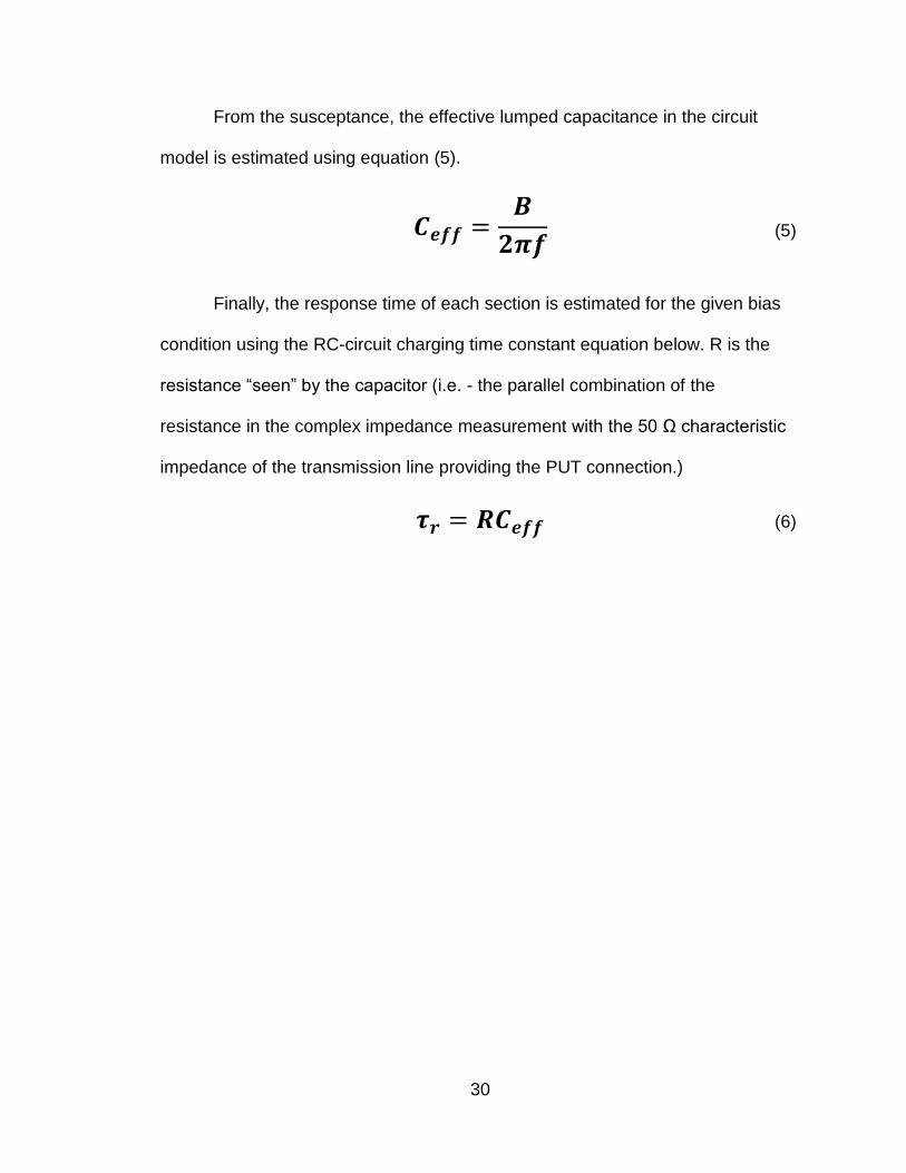
30

From the susceptance, the effective lumped capacitance in the circuit

model is estimated using equation (5).

(5)

Finally, the response time of each section is estimated for the given bias

condition using the RC-circuit charging time constant equation below. R is the

resistance “seen” by the capacitor (i.e. - the parallel combination of the

resistance in the complex impedance measurement with the 50 Ω characteristic

impedance of the transmission line providing the PUT connection.)

(6)

𝑪𝒆𝒇𝒇 =𝑩

𝟐𝝅𝒇

𝝉𝒓 = 𝑹𝑪𝒆𝒇𝒇

31

TDR Measurement Validation

To ensure the accuracy of the TDR measurements taken from both lasers

with the 9 GHz Anritsu MS4624B VNA, TDR measurements are repeated for the

BM section of the VTL-2 laser on a second TDR instrument. Response time

values derived from the frequency domain measurements on the Anritsu are also

compared to those measured in the time domain of the second measurement

setup; an HP 54754A TDR module in an Agilent mainframe is used to make the

comparable measurements.

Unlike the Anritsu VNA, the HP TDR module produces an actual step-

input and measures its reflection versus measuring the reflections of a

harmonically related set of sinusoids and using the superposition principle. This

configuration has a rise-time of approximately 49 ps which will allows the

measurement of lower response times than the Anritsu VNA.

Figure 24 is a photo of the measurement setup used. As always, the TEC

controller is energized first to maintain the waveguide temperature while lasing.

The TDR module is calibrated using the automated calibration process built into

the mainframe’s user interface to remove measurement inaccuracies introduced

by the coaxial cable and the instrument itself. The same calibration-kit loads used

in the Anritsu VNA’s calibration are used here as well.

32

Figure 24 - TDR validation instrument configuration. HP 54754A TDR module is connected to the PUT through a bias-T; the PUT is biased with the LDC current source.

It was necessary to produce a custom bias-T so non-zero bias

measurements could be made because this measurement instrument is not

capable of supplying a current bias to the PUT.

33

Figure 25 - Custom bias-T enabling non-zero current measurements with an HP 54754A TDR module. The bias connection forms a low-pass filter to prevent TDR stimuli from

reaching the bias source. The stimulus signal is transferred to the PUT via an AC coupling capacitor.

Figure 25 is a picture of the bias-T made for this measurement. The bias

path leaving the ‘T’ forms a low-pass filter with a C-L-C π-configuration; the filter

prevents high frequency content from reaching the bias source.

The TDR connection is AC shorted to the PUT connection via a small AC

coupling capacitor, allowing the PUT to have a non-zero voltage and receive a

step input from the TDR module without lifting the TDR port’s center-conductor

from ground. Figure 26 illustrates the filtering circuit components that collectively

form the bias-t.

Laser-diode controller

PUT

TDR module

Bias-T

34

Figure 26 - Bias-T circuit schematic.

Figure 27 is an example TDR measurement of the VTL-2 laser’s BM port

with a 10.1 mA bias. The response time is measured to be approximately 0.3 ns.

A dynamic resistance of 6.2 Ω is displayed explicitly on the TDR plot; Unlike the

TDR mode of the Anritsu VNA, this instrument configuration makes the

conversion from reflection coefficient to resistance automatically.

Figure 27 - TDR measurement of the VTL-2 laser's BM section at a 200 mA bias using the HP 54754A TDR module with a step-input rise time of 49 ps. A PUT response time of 0.3 ns

is observed which deviates from the Anritsu VNA measurement by only 60 ps.

τr < 0.3 ns

Rd ≈ 6.2 Ω

Horizontal scale

Step-input rise time

35

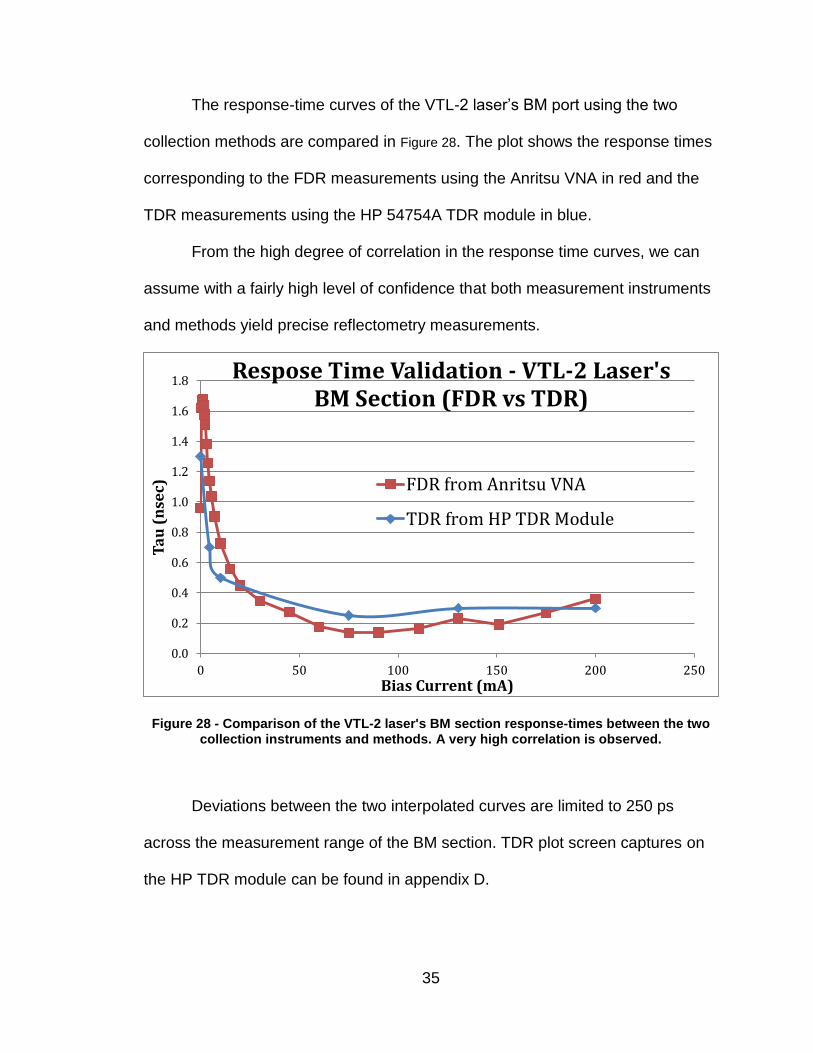
The response-time curves of the VTL-2 laser’s BM port using the two

collection methods are compared in Figure 28. The plot shows the response times

corresponding to the FDR measurements using the Anritsu VNA in red and the

TDR measurements using the HP 54754A TDR module in blue.

From the high degree of correlation in the response time curves, we can

assume with a fairly high level of confidence that both measurement instruments

and methods yield precise reflectometry measurements.

Figure 28 - Comparison of the VTL-2 laser's BM section response-times between the two collection instruments and methods. A very high correlation is observed.

Deviations between the two interpolated curves are limited to 250 ps

across the measurement range of the BM section. TDR plot screen captures on

the HP TDR module can be found in appendix D.

0.0

0.2

0.4

0.6

0.8

1.0

1.2

1.4

1.6

1.8

0 50 100 150 200 250

Ta

u (

nse

c)

Bias Current (mA)

Respose Time Validation - VTL-2 Laser's BM Section (FDR vs TDR)

FDR from Anritsu VNA

TDR from HP TDR Module

36

4. SPECTRAL CHARACTERIZATION

Tuning Maps

A wavelength-tuning map provides a visual representation of the laser’s

primary longitudinal mode as a function of the FM and BM bias currents. This

allows for the optimal tuning path for the desired linear wavelength sweep to be

identified. With the 3D surface plot of this data, anomalies that might cause non-

linearity in the wavelength sweep of the laser can be identified and avoided.

Similarly, a power-tuning map is a visual representation of the peak power

in the dominant mode of the laser’s output spectrum as a function of FM and BM

bias. With the power-tuning map, supplemental gain required by the SOA can be

easily calculated and used to realize any power profile.

Together, these tuning maps serve as a tool for identifying appropriate

spectral linewidth measurements points by illustrating bias regions that exhibit

stable single-mode operation.

The instrument configuration used to collect the tuning maps is shown in

Figure 29, below. As always, the TEC controller in the LDC is used to maintain the

waveguide temperature. The SOA and Gain sections of the laser are biased to

100 mA each to achieve stable lasing. The FM and BM ports are connected to

precision current drivers that are computer controlled through a GPIB interface.

With the MatLab function “LaserMeasurement()” I wrote for tuning map

data collection, the user defines the desired tuning map current boundaries and

resolution with the start, stop, and step arguments of the function. The output of

the laser is coupled into an Agilent 86140B OSA, also controlled by the

37

computer, to measure the power and wavelength of the dominant signal in the

laser’s output spectrum at each bias point. The function records the data

collected in an excel file called “TuningMap.xls” which is generated in the MatLab

working director when the function is run. Each time a new data collection

process is started, a new sheet is created in the excel document and titled with

the current date and time so that the dataset can be easily referenced.

In addition to the measurement of the dominant mode’s power and

wavelength at each bias point, an OSA screen capture of the laser’s output

spectrum is saved to a folder in the working directory with the same name as the

corresponding data-sheet.

Figure 29 - Instrument configuration used for tuning map collection. The user runs the MatLab function ‘LaserMeasurement()’ with the bias current start, stop, and

step/resolution values for the FM and BM precision current sources passed in the function’s argument.

38

Once a data-set is collected, the MatLab function “TuningMapper()” is

used to plot the 3D wavelength and/or power tuning surfaces for analysis. The

user is prompted with a series of questions to arrive at the desired tuning map;

the selected data-set is plotted into a 3D tuning surface by linearly interpolating

between the measured data-point vertices.

Upon execution of the function, the user is asked which excel sheet to

extract a data-set from and what tuning maps to generate; wavelength, power, or

both are the available selections. Using the cursor, the tuning surface view can

be manipulated, zoomed, and probed to analyze the laser’s tuning characteristics

within the data-set’s measurement range.

Using the MatLab function “TuningMapVid()”, a video of the tuning

surfaces can be produced in a file-type specified by the user on line 17 of the

function code. In the execution of the function, a video is created by appending a

sequence of figure images together. The view-angle is incrementally advanced

through a circular path surrounding the surface’s centroid while the view-point

elevation and field of view is decreased; this video rendering of the tuning

surface provides a novel view of the tuning surface from many angles,

elevations, and fields of view.

As with the “TuningMapper()” function, when the function is executed, the

user is prompted to select the desired data-set sheet in the “TuningMap.xls” file

to process. The user is also asked to enter the number of frames or “viewpoint

angles” to comprise the video sequence of; a number less than 500 is

recommended for larger file formats.

39

Side-Mode Suppression Ratio

The SMSR is measured at bias points of interest to investigate whether

amplified spontaneous emission (ASE) is being back-coupled from the SOA and

degrading the SMSR. Being a relative measurement of the peak-power

difference between the dominant mode and the most powerful side-mode, the

SMSR informs on the laser’s performance in applications requiring high spectral

discrimination. SS-OCT is only one such application.

In Figure 30, an example SMSR measurement is illustrated to identify the

power peak of the dominant mode, the most powerful side-mode, and the

difference between the two (i.e. - the SMSR itself).

Figure 30 - SMSR measurement example. An SMSR of greater than 27 dB is observed between the power of the dominant mode and the most powerful side-mode.

Dominant Mode

Most Powerful Side-mode

SMSR

40

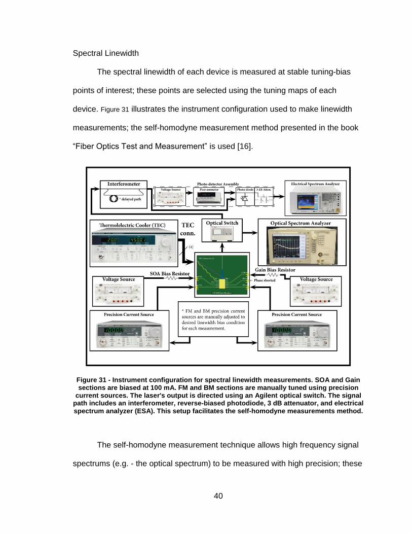
Spectral Linewidth

The spectral linewidth of each device is measured at stable tuning-bias

points of interest; these points are selected using the tuning maps of each

device. Figure 31 illustrates the instrument configuration used to make linewidth

measurements; the self-homodyne measurement method presented in the book

“Fiber Optics Test and Measurement” is used [16].

Figure 31 - Instrument configuration for spectral linewidth measurements. SOA and Gain sections are biased at 100 mA. FM and BM sections are manually tuned using precision

current sources. The laser's output is directed using an Agilent optical switch. The signal path includes an interferometer, reverse-biased photodiode, 3 dB attenuator, and electrical spectrum analyzer (ESA). This setup facilitates the self-homodyne measurements method.

The self-homodyne measurement technique allows high frequency signal

spectrums (e.g. - the optical spectrum) to be measured with high precision; these

41

spectrums are generally too high in the frequency to be accurately measured by

traditional OSAs due to their inadequate bandwidth resolutions.

The optical signal from the laser is coupled with a delayed version of itself

using the interferometer. A suitable path delay is used to ensure a valid

autocorrelation measurement can be made for the wavelengths being measured

(i.e. - 3.5 μs in this case). The autocorrelation signal is coupled to the photo-

detector assembly and the resulting modulated spectrum envelope is measured

at its full-width half maximum (FWHM) using the ESA; the modulation process

doubles the spectral width, allowing the FWHM optical spectrum to be measured

at HWHM in the electrical spectrum.

Before reliable measurements can be made, the noise floor of the Agilent

CXA signal analyzer is established as a reference. An example noise floor

measurement is presented in Figure 32.

Figure 32 - Noise floor of Agilent CXA signal analyzer used for measuring spectral linewidth and an example FWHM linewidth measurement of the Neptune laser.

42

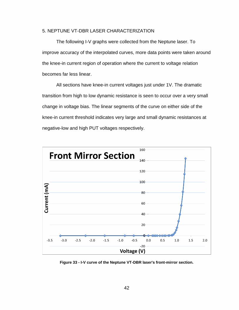
5. NEPTUNE VT-DBR LASER CHARACTERIZATION

The following I-V graphs were collected from the Neptune laser. To

improve accuracy of the interpolated curves, more data points were taken around

the knee-in current region of operation where the current to voltage relation

becomes far less linear.

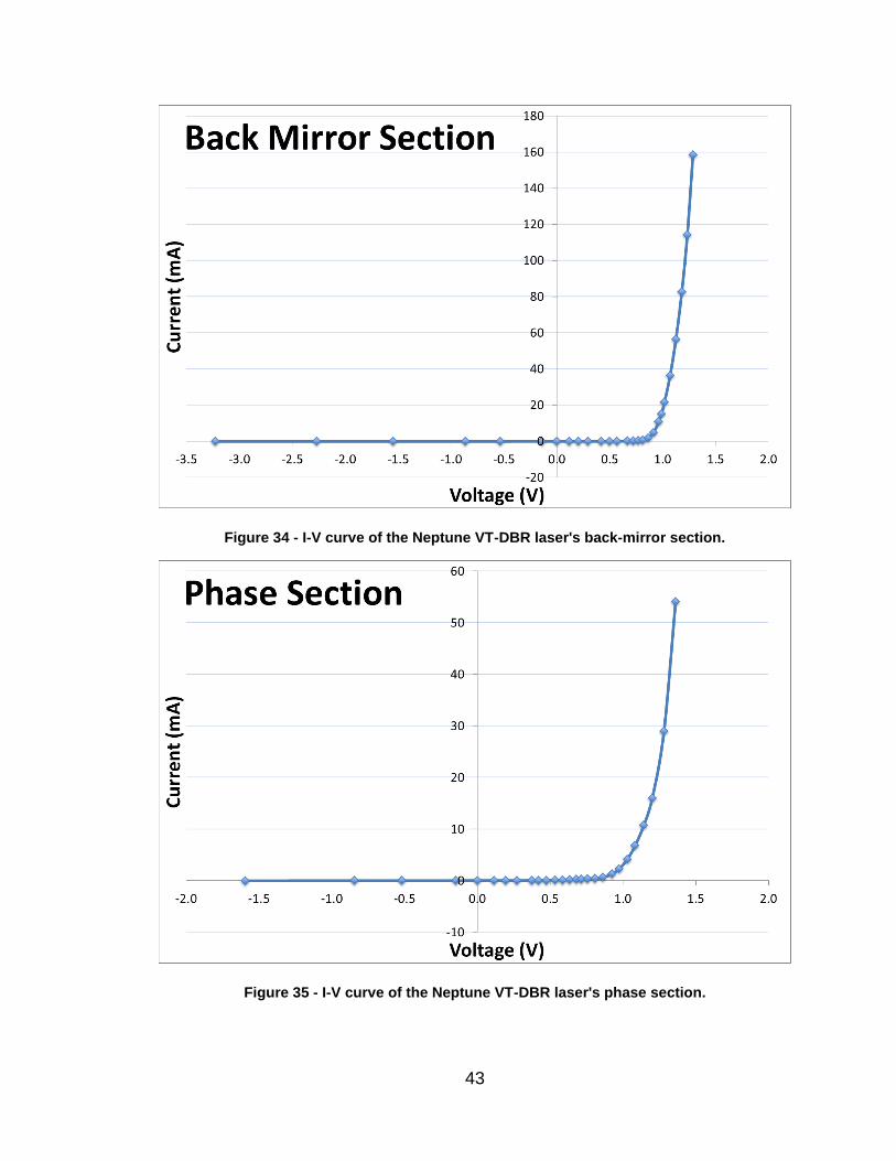
All sections have knee-in current voltages just under 1V. The dramatic

transition from high to low dynamic resistance is seen to occur over a very small

change in voltage bias. The linear segments of the curve on either side of the

knee-in current threshold indicates very large and small dynamic resistances at

negative-low and high PUT voltages respectively.

Figure 33 - I-V curve of the Neptune VT-DBR laser's front-mirror section.

43

Figure 34 - I-V curve of the Neptune VT-DBR laser's back-mirror section.

Figure 35 - I-V curve of the Neptune VT-DBR laser's phase section.

44

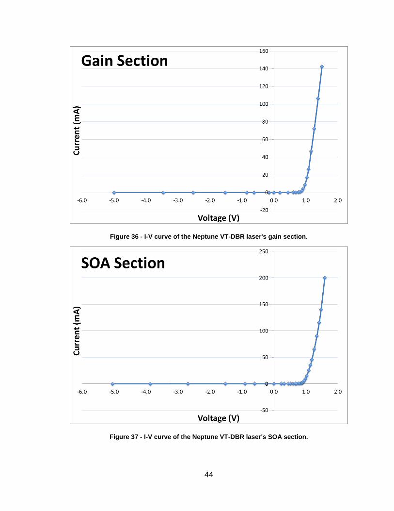
Figure 36 - I-V curve of the Neptune VT-DBR laser's gain section.

Figure 37 - I-V curve of the Neptune VT-DBR laser's SOA section.

45

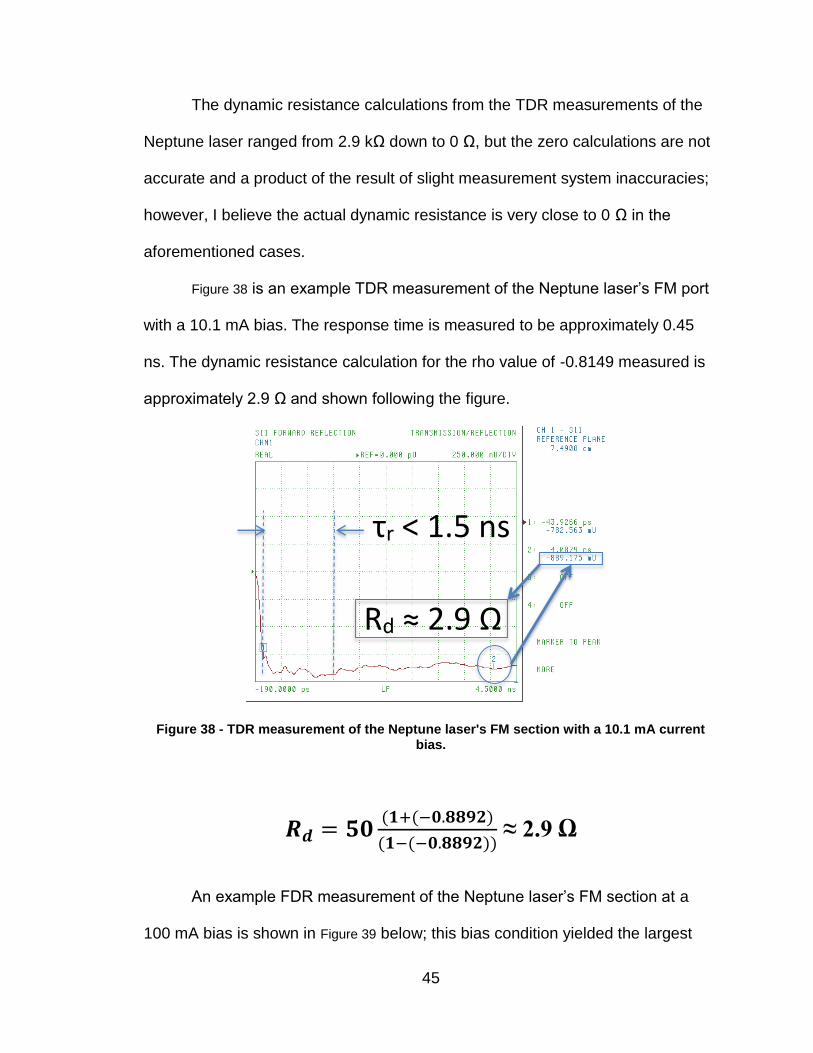
The dynamic resistance calculations from the TDR measurements of the

Neptune laser ranged from 2.9 kΩ down to 0 Ω, but the zero calculations are not

accurate and a product of the result of slight measurement system inaccuracies;

however, I believe the actual dynamic resistance is very close to 0 Ω in the

aforementioned cases.

Figure 38 is an example TDR measurement of the Neptune laser’s FM port

with a 10.1 mA bias. The response time is measured to be approximately 0.45

ns. The dynamic resistance calculation for the rho value of -0.8149 measured is

approximately 2.9 Ω and shown following the figure.

Figure 38 - TDR measurement of the Neptune laser's FM section with a 10.1 mA current bias.

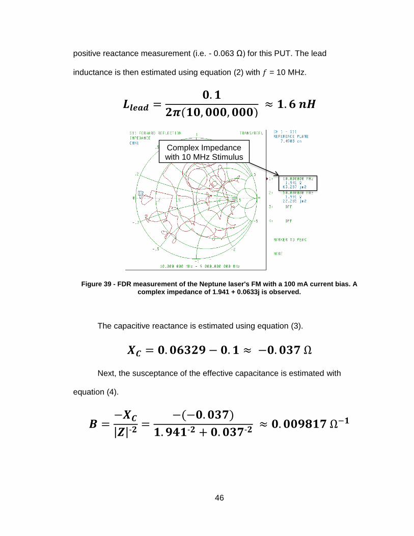
An example FDR measurement of the Neptune laser’s FM section at a

100 mA bias is shown in Figure 39 below; this bias condition yielded the largest

𝑹𝒅 = 𝟓𝟎(𝟏+(−𝟎.𝟖𝟖𝟗𝟐)

(𝟏−(−𝟎.𝟖𝟖𝟗𝟐)) ≈ 2.9 Ω

τr < 1.5 ns

Rd ≈ 2.9 Ω

46

positive reactance measurement (i.e. - 0.063 Ω) for this PUT. The lead

inductance is then estimated using equation (2) with 𝑓 = 10 MHz.

Figure 39 - FDR measurement of the Neptune laser's FM with a 100 mA current bias. A complex impedance of 1.941 + 0.0633j is observed.

The capacitive reactance is estimated using equation (3).

Next, the susceptance of the effective capacitance is estimated with

equation (4).

𝑳𝒍𝒆𝒂𝒅 =𝟎. 𝟏

𝟐𝝅(𝟏𝟎, 𝟎𝟎𝟎, 𝟎𝟎𝟎) ≈ 𝟏. 𝟔 𝒏𝑯

𝑿𝑪 = 𝟎. 𝟎𝟔𝟑𝟐𝟗 − 𝟎. 𝟏 ≈ −𝟎. 𝟎𝟑𝟕 Ω

𝑩 =−𝑿𝑪

|𝒁|-𝟐=

−(−𝟎. 𝟎𝟑𝟕)

𝟏. 𝟗𝟒𝟏-𝟐 + 𝟎. 𝟎𝟑𝟕-𝟐 ≈ 𝟎. 𝟎𝟎𝟗𝟖𝟏𝟕 Ω−𝟏

Complex Impedance with 10 MHz Stimulus

47

Then, the effective capacitance is calculated with equation (5).

Finally, the response time for this bias condition is calculated using

equation (6).

The above RLC calculations are performed for every bias condition of

each PUT and presented in appendix B. Figure 40 plots the bias dependent

response times of each Neptune laser section.

Figure 40 - Neptune laser's response times versus bias current for each PUT.

Figure 41 is a picture of the Neptune laser’s wavelength tuning map with FM

and BM currents ranging from 0 to 100 mA at an increment of 1 mA along each

0.0

0.2

0.4

0.6

0.8

1.0

1.2

1.4

1.6

1.8

2.0

0 20 40 60 80 100 120 140 160

Ta

u (

ns)

Bias Current (mA)

Tau vs Bias Current - Neptune Laser

FM

BM

PM

SOA

𝑪𝒆𝒇𝒇 =𝟎. 𝟎𝟎𝟗𝟖𝟏𝟕

𝟐𝝅(𝟏𝟎, 𝟎𝟎𝟎, 𝟎𝟎𝟎) ≈ 𝟏𝟓𝟔 𝒑𝑭

𝝉𝒔 = 𝑹𝑪𝒆𝒇𝒇 ≈ 𝟏. 𝟖𝟕 ∗ 𝟏𝟓𝟔𝑬−𝟏𝟐 ≈ 𝟎. 𝟐𝟗 𝒏𝒔

48

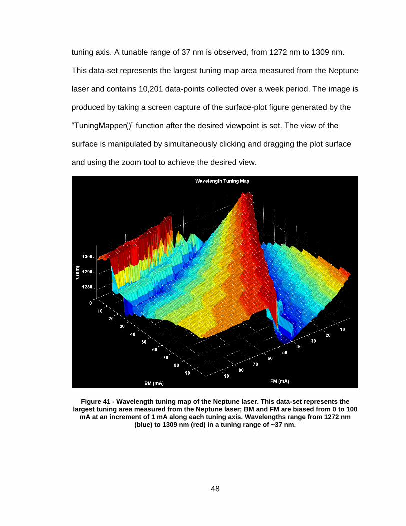
tuning axis. A tunable range of 37 nm is observed, from 1272 nm to 1309 nm.

This data-set represents the largest tuning map area measured from the Neptune

laser and contains 10,201 data-points collected over a week period. The image is

produced by taking a screen capture of the surface-plot figure generated by the

“TuningMapper()” function after the desired viewpoint is set. The view of the

surface is manipulated by simultaneously clicking and dragging the plot surface

and using the zoom tool to achieve the desired view.

Figure 41 - Wavelength tuning map of the Neptune laser. This data-set represents the largest tuning area measured from the Neptune laser; BM and FM are biased from 0 to 100

mA at an increment of 1 mA along each tuning axis. Wavelengths range from 1272 nm (blue) to 1309 nm (red) in a tuning range of ~37 nm.

49

The FM current, BM current, and dominant mode wavelength respectively

define the X, Y, and Z position on the tuning map. The surface is also color

coded to reflect the wavelength at a given point.

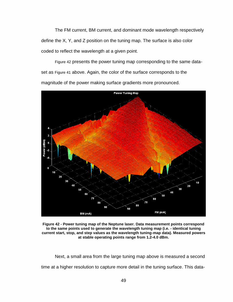
Figure 42 presents the power tuning map corresponding to the same data-

set as Figure 41 above. Again, the color of the surface corresponds to the

magnitude of the power making surface gradients more pronounced.

Figure 42 - Power tuning map of the Neptune laser. Data measurement points correspond to the same points used to generate the wavelength tuning map (i.e. - identical tuning

current start, stop, and step values as the wavelength tuning-map data). Measured powers at stable operating points range from 1.2-4.0 dBm.

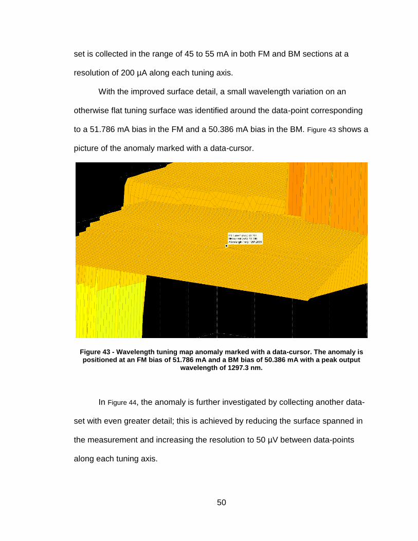
Next, a small area from the large tuning map above is measured a second

time at a higher resolution to capture more detail in the tuning surface. This data-

50

set is collected in the range of 45 to 55 mA in both FM and BM sections at a

resolution of 200 µA along each tuning axis.

With the improved surface detail, a small wavelength variation on an

otherwise flat tuning surface was identified around the data-point corresponding

to a 51.786 mA bias in the FM and a 50.386 mA bias in the BM. Figure 43 shows a

picture of the anomaly marked with a data-cursor.

Figure 43 - Wavelength tuning map anomaly marked with a data-cursor. The anomaly is positioned at an FM bias of 51.786 mA and a BM bias of 50.386 mA with a peak output

wavelength of 1297.3 nm.

In Figure 44, the anomaly is further investigated by collecting another data-

set with even greater detail; this is achieved by reducing the surface spanned in

the measurement and increasing the resolution to 50 µV between data-points

along each tuning axis.

51

Significantly more detail is captured in this plot; the surface appears very

rippled, but these small deviations are all less than 3 pm and might be caused by

performance limitations (i.e. - temperature fluctuations up to +/- 0.05 degrees

Celsius) in the TEC controller or measurement device itself.

Figure 44 - Improved image of wavelength tuning map anomaly. Tuning map span is reduced to less than 2 mA along each tuning axis and the resolution is improved to 50 µA

between data-points.

The larger ripple running parallel to the BM axis introduces a measured

wavelength deviation of >15 pm; one might suspect its cause to be temperature

fluctuations in the waveguide, but the fact it appears in two data-sets collected at

different times makes that hypothesis far less likely. Anomalies of this size must

be avoided to reduce points of non-linearity in a SS-OCT wavelength sweep.

I wrote the MatLab data-collection function such that data-points are

gathered along the BM axis and sequenced along the entire BM range specified

before iterating to the next FM current; therefore, I suspect fluctuations in

environmental variables that affect the output wavelength (e.g. - cavity

52

stress/strain) will manifest similar anomalies that run along BM axis. However, I

do not believe it to be the cause here.

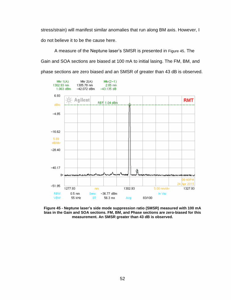
A measure of the Neptune laser’s SMSR is presented in Figure 45. The

Gain and SOA sections are biased at 100 mA to initial lasing. The FM, BM, and

phase sections are zero biased and an SMSR of greater than 43 dB is observed.

Figure 45 - Neptune laser’s side mode suppression ratio (SMSR) measured with 100 mA bias in the Gain and SOA sections. FM, BM, and Phase sections are zero-biased for this

measurement. An SMSR greater than 43 dB is observed.

53

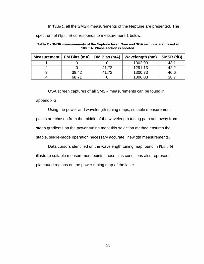
In Table 2, all the SMSR measurements of the Neptune are presented. The

spectrum of Figure 45 corresponds to measurement 1 below.

Table 2 - SMSR measurements of the Neptune laser. Gain and SOA sections are biased at 100 mA. Phase section is shorted.

Measurement FM Bias (mA) BM Bias (mA) Wavelength (nm) SMSR (dB)

1 0 0 1302.93 43.1

2 0 41.72 1291.13 42.2

3 38.42 41.72 1300.73 40.6

4 68.71 0 1306.03 38.7

OSA screen captures of all SMSR measurements can be found in

appendix G.

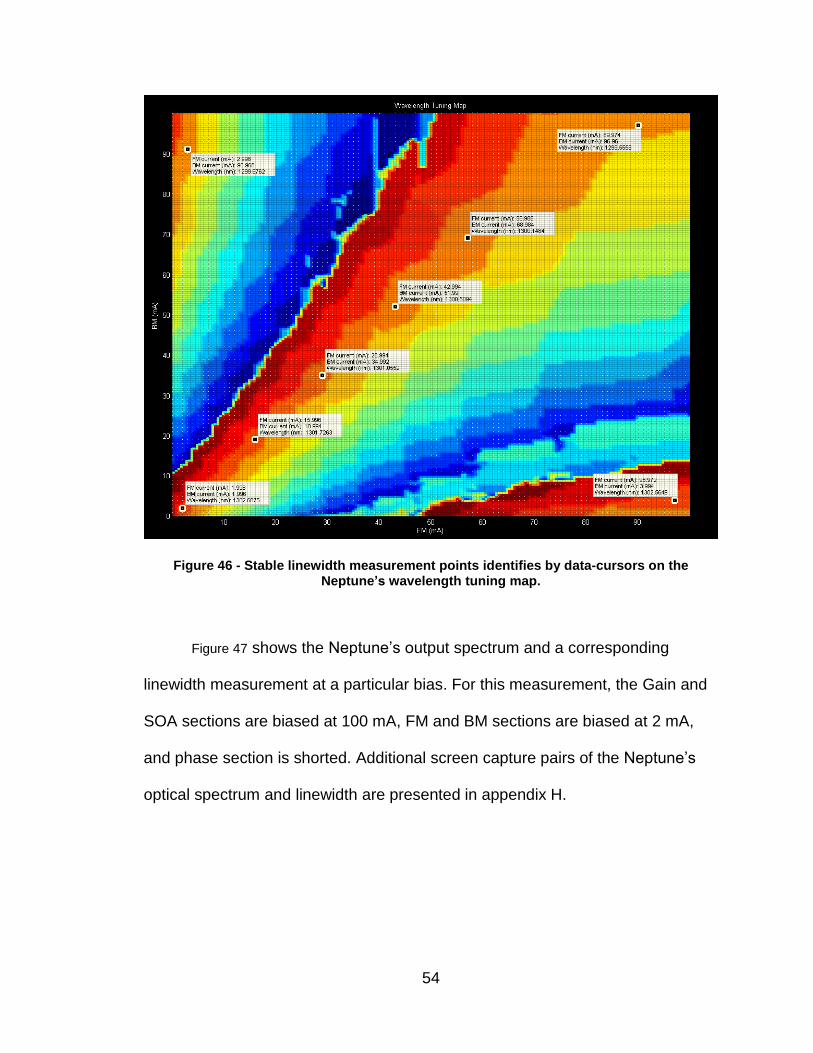
Using the power and wavelength tuning maps, suitable measurement

points are chosen from the middle of the wavelength tuning path and away from

steep gradients on the power tuning map; this selection method ensures the

stable, single-mode operation necessary accurate linewidth measurements.

Data cursors identified on the wavelength tuning map found in Figure 46

illustrate suitable measurement points; these bias conditions also represent

plateaued regions on the power tuning map of the laser.

54

Figure 46 - Stable linewidth measurement points identifies by data-cursors on the Neptune’s wavelength tuning map.

Figure 47 shows the Neptune’s output spectrum and a corresponding

linewidth measurement at a particular bias. For this measurement, the Gain and

SOA sections are biased at 100 mA, FM and BM sections are biased at 2 mA,

and phase section is shorted. Additional screen capture pairs of the Neptune’s

optical spectrum and linewidth are presented in appendix H.

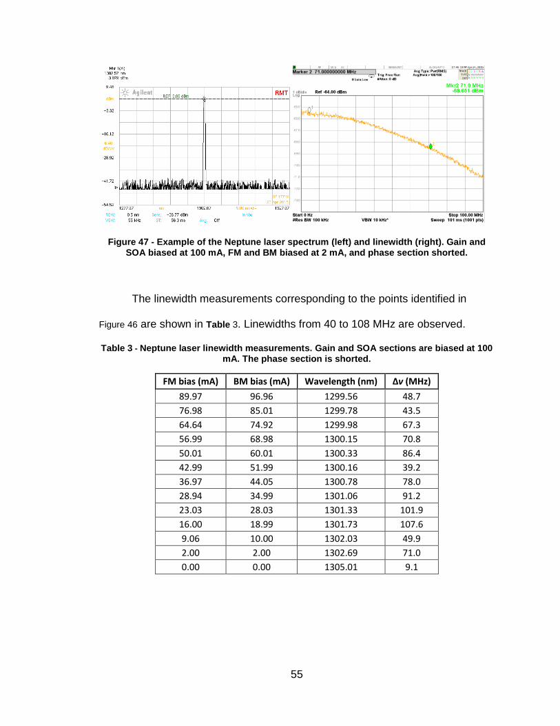
55

Figure 47 - Example of the Neptune laser spectrum (left) and linewidth (right). Gain and SOA biased at 100 mA, FM and BM biased at 2 mA, and phase section shorted.

The linewidth measurements corresponding to the points identified in

Figure 46 are shown in Table 3. Linewidths from 40 to 108 MHz are observed.

Table 3 - Neptune laser linewidth measurements. Gain and SOA sections are biased at 100 mA. The phase section is shorted.

FM bias (mA) BM bias (mA) Wavelength (nm) Δv (MHz)

89.97 96.96 1299.56 48.7

76.98 85.01 1299.78 43.5

64.64 74.92 1299.98 67.3

56.99 68.98 1300.15 70.8

50.01 60.01 1300.33 86.4

42.99 51.99 1300.16 39.2

36.97 44.05 1300.78 78.0

28.94 34.99 1301.06 91.2

23.03 28.03 1301.33 101.9

16.00 18.99 1301.73 107.6

9.06 10.00 1302.03 49.9

2.00 2.00 1302.69 71.0

0.00 0.00 1305.01 9.1

56

Additional linewidth measurements of the Neptune laser are presented in

Table 4 and Table 5. Measurements in Table 4 are made with the FM section zero-

biased. Linewidths range from 4 to 28 MHz.

Table 4 - Neptune laser linewidth measurements. Gain and SOA sections are biased at 100 mA. The phase and FM sections are shorted.

BM bias (mA) Wavelength (nm) Δv (MHz)

99.98 1302.88 7.3

89.98 1299.88 27.2

80.46 1299.98 11.9

70.00 1296.93 25.5

60.05 1296.98 4.8

50.13 1294.08 8.4

40.07 1291.18 6.8

30.59 1288.28 3.6

20.00 1282.53 16.8

10.20 1276.93 25.3

5.02 1308.88 27.7

Measurements in Table 5 are made with the BM section zero-biased.

Linewidths range from 6 to 130 MHz. From the results, the FM current bias

appears to be more influential on the spectral linewidth of the Neptune laser.

Table 5 - Neptune laser linewidth measurements. Gain and SOA sections are biased at 100 mA. The phase and BM sections are shorted.

FM bias (mA) Wavelength (nm) Δv (MHz)

99.96 1299.66 18.6

90.05 1299.61 5.5

80.00 1302.76 39.9

68.04 1305.96 57.4

59.22 1306.06 40.6

51.21 1309.26 45.4

37.51 1282.96 79.3

31.85 1277.66 134.2

19.71 1286.71 104.6

10.11 1293.16 120.7

6.02 1296.41 130.0

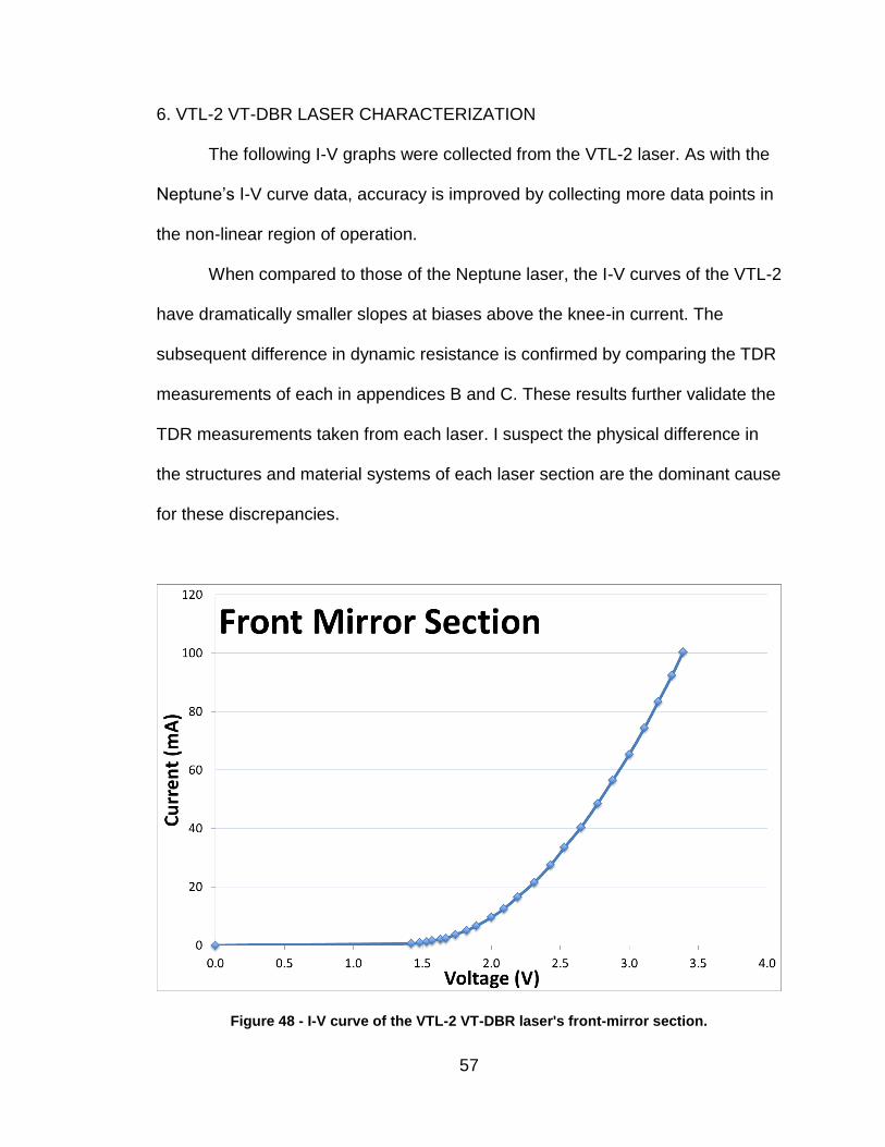
57

6. VTL-2 VT-DBR LASER CHARACTERIZATION

The following I-V graphs were collected from the VTL-2 laser. As with the

Neptune’s I-V curve data, accuracy is improved by collecting more data points in

the non-linear region of operation.

When compared to those of the Neptune laser, the I-V curves of the VTL-2

have dramatically smaller slopes at biases above the knee-in current. The

subsequent difference in dynamic resistance is confirmed by comparing the TDR

measurements of each in appendices B and C. These results further validate the

TDR measurements taken from each laser. I suspect the physical difference in

the structures and material systems of each laser section are the dominant cause

for these discrepancies.

Figure 48 - I-V curve of the VTL-2 VT-DBR laser's front-mirror section.

58

Figure 49 - I-V curve of the VTL-2 VT-DBR laser's back-mirror section.

Figure 50 - I-V curve of the VTL-2 VT-DBR laser's phase section.

59

Figure 51 - I-V curve of the VTL-2 VT-DBR laser's gain section.

Figure 52 - I-V curve of the VTL-2 VT-DBR laser's SOA section.

60

Figure 53 is an example TDR measurement of the VTL-2 laser’s BM port

with a 10.1 mA bias. The response time is measured to be approximately 0.7 ns.

The dynamic resistance calculation for the rho value of -0.3220 measured is

approximately 25.6 Ω and shown following the figure.

Figure 53 - TDR measurement of the VTL-2 laser's BM section with a 10.1 mA current bias.

An example FDR measurement of the VTL-2 laser’s BM section at a 90.1

mA bias is shown in Figure 54 below; this bias condition yields the largest positive

reactance (i.e. - 0.063 Ω) for this PUT. The lead inductance is then estimated

using equation (2) where 𝑓 = 10 MHz.

𝑹𝒅 = 𝟓𝟎(𝟏+(−𝟎.𝟑𝟐𝟐𝟎)

(𝟏−(−𝟎.𝟑𝟐𝟐𝟎)) ≈ 25.6 Ω

𝑳𝒍𝒆𝒂𝒅 =𝟏. 𝟎

𝟐𝝅(𝟏𝟎, 𝟎𝟎𝟎, 𝟎𝟎𝟎) ≈ 𝟏𝟔 𝒏𝑯

τr < 0.7 ns

Rd ≈ 25.6 Ω

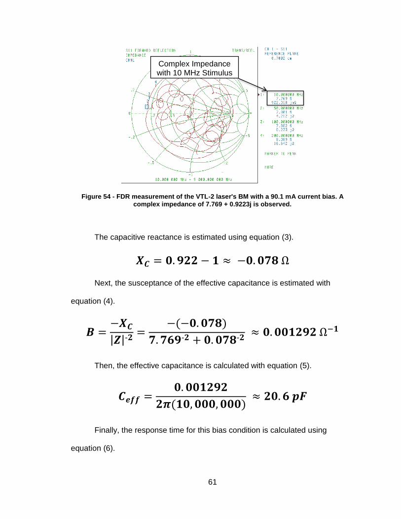
61

Figure 54 - FDR measurement of the VTL-2 laser's BM with a 90.1 mA current bias. A complex impedance of 7.769 + 0.9223j is observed.

The capacitive reactance is estimated using equation (3).

Next, the susceptance of the effective capacitance is estimated with

equation (4).

Then, the effective capacitance is calculated with equation (5).

Finally, the response time for this bias condition is calculated using

equation (6).

𝑿𝑪 = 𝟎. 𝟗𝟐𝟐 − 𝟏 ≈ −𝟎. 𝟎𝟕𝟖 Ω

𝑩 =−𝑿𝑪

|𝒁|-𝟐=

−(−𝟎. 𝟎𝟕𝟖)

𝟕. 𝟕𝟔𝟗-𝟐 + 𝟎. 𝟎𝟕𝟖-𝟐 ≈ 𝟎. 𝟎𝟎𝟏𝟐𝟗𝟐 Ω−𝟏

𝑪𝒆𝒇𝒇 =𝟎. 𝟎𝟎𝟏𝟐𝟗𝟐

𝟐𝝅(𝟏𝟎, 𝟎𝟎𝟎, 𝟎𝟎𝟎) ≈ 𝟐𝟎. 𝟔 𝒑𝑭

Complex Impedance with 10 MHz Stimulus

62

The above RLC calculations are performed for every bias condition of

each PUT and presented in appendix C.

A measure of the VTL-2 laser’s SMSR is presented in Figure 45. The Gain

and SOA sections are biased at 100 mA to initial lasing. The FM, BM, and phase

sections are zero biased and an SMSR of greater than 33 dB is observed.

Figure 55 - VTL-2 laser’s side mode suppression ratio (SMSR) measured with 100 mA bias in the Gain and SOA sections. FM is biased at 40.4 mA, BM is zero biased, and the phase

section is shorted. A SMSR greater than 43 dB is observed.

In Table 6, all the SMSR measurements for the VTL-2 are presented. The

spectrum of Figure 55 corresponds to measurement 3 below.

𝝉𝒔 = 𝑹𝑪𝒆𝒇𝒇 ≈ 𝟔. 𝟕𝟐 ∗ 𝟐𝟎. 𝟔𝑬−𝟏𝟐 ≈ 𝟎. 𝟏𝟒 𝒏𝒔

63

Table 6 - SMSR measurements of the VTL-2 laser. Gain and SOA sections are biased at 100 mA. Phase section is shorted.

Measurement FM Bias (mA) BM Bias (mA) Wavelength (nm) SMSR (dB)

1 0 40.95 1067.17 32.9

2 40.39 94.68 1074.57 30.3

3 40.38 0 1081.57 33.5

OSA screen captures for each SMSR measurement can be found in

appendix I.

Figure 56 shows the VTL-2’s output spectrum and a corresponding

linewidth measurement at a particular bias. For this measurement, the Gain and

SOA sections are biased at 100 mA, the FM and BM sections are biased at 79

mA, and the phase section is shorted. Additional OSA and linewidth

measurement screen capture pairs are presented in appendix J.

Figure 56 - Example of the VTL-2 laser spectrum (left) and linewidth (right). Gain and SOA biased at 100 mA, FM and BM biased at 79 mA, and phase section shorted.

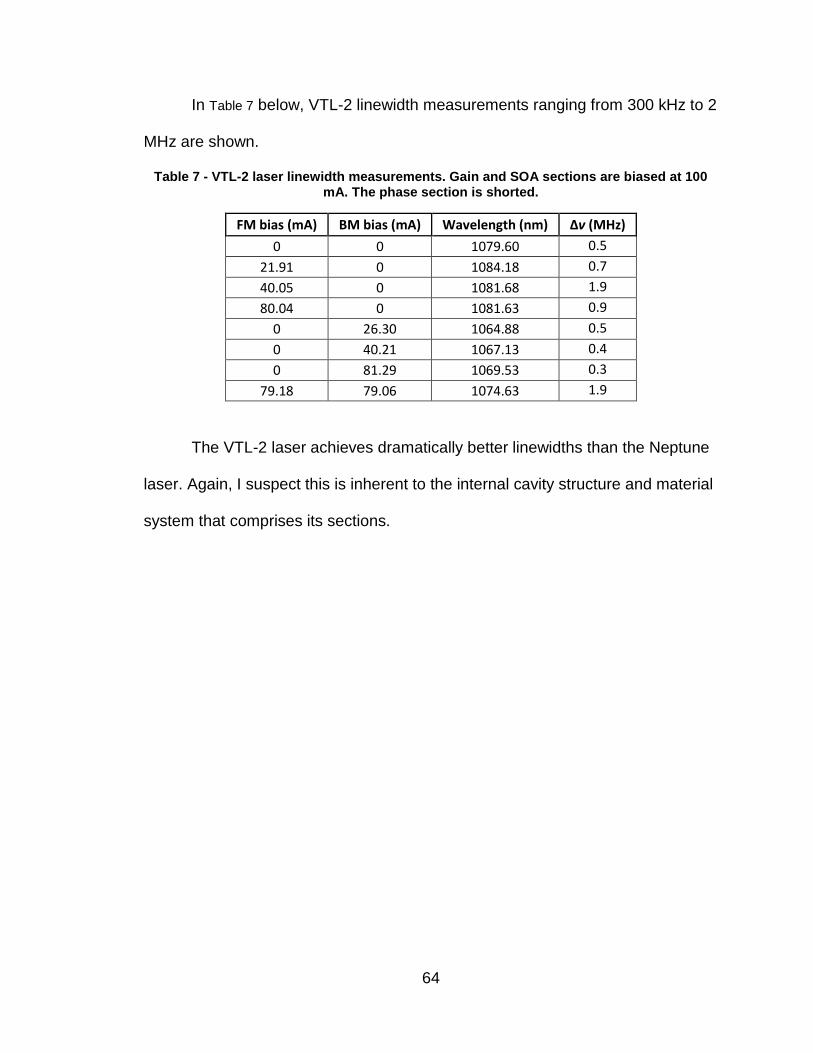
64

In Table 7 below, VTL-2 linewidth measurements ranging from 300 kHz to 2

MHz are shown.

Table 7 - VTL-2 laser linewidth measurements. Gain and SOA sections are biased at 100 mA. The phase section is shorted.

FM bias (mA) BM bias (mA) Wavelength (nm) Δv (MHz)

0 0 1079.60 0.5

21.91 0 1084.18 0.7

40.05 0 1081.68 1.9

80.04 0 1081.63 0.9

0 26.30 1064.88 0.5

0 40.21 1067.13 0.4

0 81.29 1069.53 0.3

79.18 79.06 1074.63 1.9

The VTL-2 laser achieves dramatically better linewidths than the Neptune

laser. Again, I suspect this is inherent to the internal cavity structure and material

system that comprises its sections.

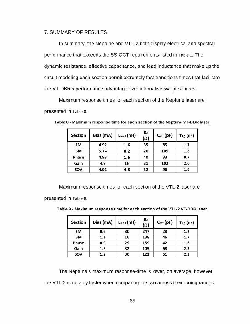
65

7. SUMMARY OF RESULTS

In summary, the Neptune and VTL-2 both display electrical and spectral

performance that exceeds the SS-OCT requirements listed in Table 1. The

dynamic resistance, effective capacitance, and lead inductance that make up the

circuit modeling each section permit extremely fast transitions times that facilitate

the VT-DBR’s performance advantage over alternative swept-sources.

Maximum response times for each section of the Neptune laser are

presented in Table 8.

Table 8 - Maximum response time for each section of the Neptune VT-DBR laser.

Section Bias (mA) Llead (nH) Rd (Ω)

Ceff (pF) τRC (ns)

FM 4.92 1.6 35 85 1.7

BM 5.74 0.2 26 109 1.8

Phase 4.93 1.6 40 33 0.7

Gain 4.9 16 31 102 2.0

SOA 4.92 4.8 32 96 1.9

Maximum response times for each section of the VTL-2 laser are

presented in Table 9.

Table 9 - Maximum response time for each section of the VTL-2 VT-DBR laser.

Section Bias (mA) Llead (nH) Rd (Ω)

Ceff (pF) τRC (ns)

FM 0.6 30 247 28 1.2

BM 1.1 16 138 46 1.7

Phase 0.9 29 159 42 1.6

Gain 1.5 32 105 68 2.3

SOA 1.2 30 122 61 2.2

The Neptune’s maximum response-time is lower, on average; however,

the VTL-2 is notably faster when comparing the two across their tuning ranges.

66

Measured I-V curves of each device helped to validate the dynamic

resistance calculations from the TDR response data and report the section

voltage of each section under bias so the drive circuitry can be designed

according to these specifications.

The tuning maps collected from the Neptune helped identify the optimal

tuning path of the laser and revealed anomalies in the tuning surface that should

be avoided to minimize the invalid data-points associated with a SS-OCT sweep.

Additionally, the maps aided the selection of relevant linewidth measurement

points by showing where stable modes of operation in the tuning path could be

achieved.

The side mode suppression ratio of the Neptune is typical of tunable DBR

lasers with an average SMSR > 41 dB. The SMSR of the VTL-2 is significantly

less than that of the Neptune at an average SMSR just above 32 dB. The

SMSRs of both lasers are well above the 25 dB value listed in Table 1. This

additional spectral discrimination results in improved OCT image quality.

The Neptune laser’s measured linewidth did not exceed 130 MHz and its

average measure was 51.6 MHz which corresponds to an average coherence

length of 1.85 meters. The VTL-2 linewidths were substantially lower, with a

maximum of 1.9 MHz and an average of only 900 kHz; this ridiculously low

linewidth, comparable to those found in mode-locked lasers, affords the VTL-2 an

average coherence length of 106 meters. The linewidths of both lasers make

them great swept-sources for OCT, but the exceptionally long coherence length

of the VTL-2 make it an ideal solution for a number of other applications that

67

require a longer coherence length (e.g. - remote sensing, seismology, and

topography contour mapping).

In conclusion, both lasers exhibit superb performance characteristics that

validate them as excellent light sources for use in SS-OCT. Their superior

performance, robust set of applications, and predictably low cost at increased

economies of scale make VT-DBR lasers the tunable light sources of the future.

68

8. FUTURE WORK

In following my work, a future scholar might use the TDR, FDR, and RLC

data I have collected to develop an improved circuit model of each laser section.

The bias dependent circuit models I have used to estimate the VT-DBR laser’s

response times are valid at discrete bias points; by attempting to produce a

mathematical model that describes the electrical characteristics of each laser

section continuously with respect to their bias current, the tuning limitations of the

VT-DBR lasers can be better understood and analyzed; from this, design

changes that improve tuning response time and accuracy may become evident.

The development of an automated linewidth/SMSR collection system

would also be a great contribution to the advancement of these lasers; because

their values dramatically impact OCT image quality and fluctuate across the

tuning range of the device, it is desirable to have a more continuous

understanding of these performance parameters.

A measure of the amplitude deviation in the output wavelength or relative

intensity noise (RIN) is also desirable.

Another useful measurement involves lasing at a stable mode and driving

the gain/SOA section of the laser with a swept sinusoid; at some increased

frequency, the optical output power of the laser is reduced by half due to the

bandwidth limitations of the section; this important -3 dB measurement identifies

the speed at which the laser’s power can be modulated.

Similar to the amplitude modulations measurement above, frequency

modulation limitations of the laser’s output are also very important. By applying a

69

swept sinusoid to each tuning section of the laser and measuring the reduction

on the tuning span as a function of tuning signal frequency, the bandwidth of

each tuning port can be calculated and used to estimate sweep speed limits.

Practical demonstrations of these lasers, like those performed with earlier

VT-DBR designs, are huge steps towards validating the niche of each and

bringing them to market. Given the promising future of the VT-DBR design, even

a crude demonstration would be a significant contribution toward the

advancement of photonics.

Relative intensity noise (RIN) measurements of the optical output are also

very important. Although difficult to measure over the finite noise in the driving

source, this measure is particularly important to fiber-optic communications and

remote-sensing.

I hope my MatLab functions will be used by future graduate students to aid

their research and inspire their curiosity in these fascinating devices. The tuning

maps they produce aid the development of a fundamental knowledge in the

operation of VT-DBRs and present a useful tool to better understanding them.

70

BIBLIOGRAPHY

[1] P.P. Sorokin and J.R. Lankard, "Stimulated Emission Observed from an

Organic Dye, Chloro-aluminum Phthalocyanine," IBM Journal of

Research and Development, vol. 10, no. 2, pp. 162-163, March 1966.

[2] Leslie Wright. (2015, May) www.fineartradiography.com. [Online].

http://www.fineartradiography.com/hobbies/lasers/dye/

[3] F.J. Duarte and L.W. Hillman, "Narrow-linewidth Pulsed Dye Laser

Oscillators," in Dye Laser Principles: With Applications. San Diego,

United States: Academic Press, Inc., 1990, ch. 4, pp. 134-170.

[4] Dennis Derickson et al., "SGDBR single-chip wavelength tunable lasers for

swept source OCT," in SPIE Digital Library, San Jose, 2008.

[5] Michael P Minneman, Jason Ensher, Michael Crawford, and Dennis

Derickson, "All-Semiconductor High-Speed Akinetic Swept-Source for

OCT," SPIE-OSA-IEEE Asia Communications and Photonics, vol.

8311, 2011.

[6] M. Bonesi et al., "Akenetic all-semiconductor programmable swept-source at

1550 nm and 1310 nm with centimeter coherence length," OSA -

Optics Express, vol. 22, no. 3, Jan 2014.

[7] Helena Jelinkova, Lasers for Medical Applications: Diagnostics, Therapy and

Surgery, 1st ed., Helena Jelinkova, Ed. Philadelphia, USA: Woodhead

, 2013.

[8] Wolfgang Drexler, "Where is retinal optical coherence tomography

71

heading?," SPIE Newsroom, vol. 10.1117/2.1200903.1584, 2009.

[9] Paulo Stanga. (2015, April) YouTube.com. [Online].

https://www.youtube.com/watch?v=r-PerZ7Vg6I

[10] James Strong. (2015, April) Ophthalmic Photographers' Society - Eye

Imaging Experts. [Online]. http://www.opsweb.org/?page=RetinalOCT

[11] S.M.R. Motaghian Nezam, "High-speed polygon-scanner-based wavelength-

swept laser source in the telescope-less configuration with

applications in optical coherence tomography," Optics Letters, vol. 33,

no. 15, August 2008.

[12] Santec Inc. (2015, May) Santec.com. [Online].

http://www.santec.com/en/products/oct/hsl-11002100

[13] Santec Inc. (2015, May) Santec.com. [Online].

http://www.santec.com/en/products/oct/hsl-1020

[14] Thorlabs Inc.. (2015, May) Thorlabs.com. [Online].

http://www.thorlabs.us/newgrouppage9.cfm?objectgroup_id=6473

[15] Desmond Talkington, "Characterization and Modeling of an O-Band 1310 nm

Sampled-Grating Distributed Bragg Reflector (SG-DBR) Laser for

Optical Coherence Tomography (OCT) Applications," California

Polytechnic State University, San Luis Obispo, Thesis 2013.

[16] Dennis Derickson, Fiber Optic Test and Measurement, 1st ed., Dennis

Derickson, Ed. Upper Saddle River, United States of America:

Printice-Hall Inc., 1998.

72

APPENDICES

Appendix A: Butterfly Laser Package Pinout Diagram

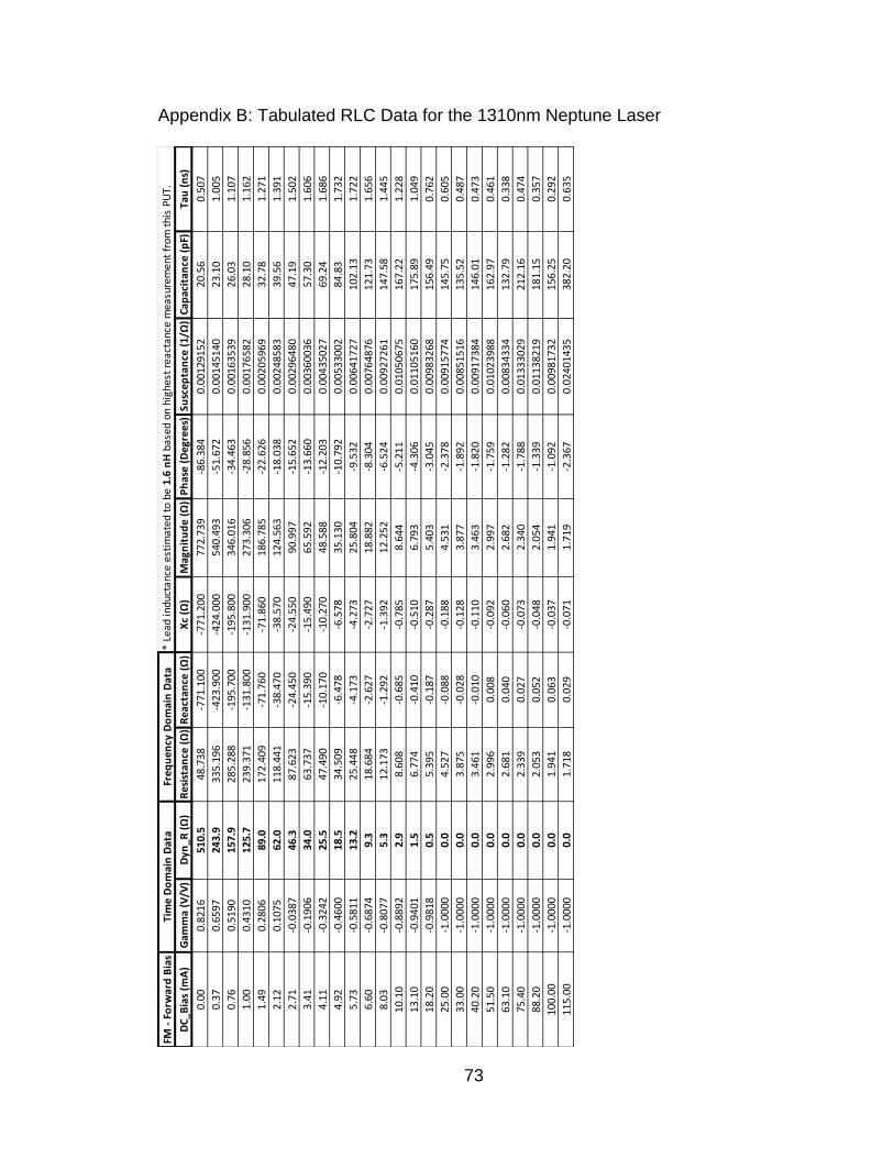
73

Appendix B: Tabulated RLC Data for the 1310nm Neptune Laser

FM -

Fo

rwar

d B

ias

* Le

ad in

duct

ance

est

imat

ed t

o be

1.6

nH

bas

ed o

n hi

ghes

t re

acta

nce

mea

sure

men

t fr

om t

his

PUT.

DC_

Bia

s (m

A)

Gam

ma

(V/V

)D

yn_R

(Ω

)R

esis

tan

ce (

Ω)

Rea

ctan

ce (

Ω)

Xc

(Ω)

Mag

nit

ud

e (Ω

)P

has

e (D

egre

es)

Susc

epta

nce

(1/

Ω)

Cap

acit

ance

(p

F)Ta

u (

ns)

0.00

0.82

1651

0.5

48.7

38-7

71.1

00-7

71.2

0077

2.73

9-8

6.38

40.

0012

9152

20.5

60.

507

0.37

0.65

9724

3.9

335.

196

-423

.900

-424

.000

540.

493

-51.

672

0.00

1451

4023

.10

1.00

5

0.76

0.51

9015

7.9

285.

288

-195

.700

-195

.800

346.

016

-34.

463

0.00

1635

3926

.03

1.10

7

1.00

0.43

1012

5.7

239.

371

-131

.800

-131

.900

273.

306

-28.

856

0.00

1765

8228

.10

1.16

2

1.49

0.28

0689

.017

2.40

9-7

1.76

0-7

1.86

018

6.78

5-2

2.62

60.

0020

5969

32.7

81.

271

2.12

0.10

7562

.011

8.44

1-3

8.47

0-3

8.57

012

4.56

3-1

8.03

80.

0024

8583

39.5

61.

391

2.71

-0.0

387

46.3

87.6

23-2

4.45

0-2

4.55

090

.997

-15.

652

0.00

2964

8047

.19

1.50

2

3.41

-0.1

906

34.0

63.7

37-1

5.39

0-1

5.49

065

.592

-13.

660

0.00

3600

3657

.30

1.60

6

4.11

-0.3

242

25.5

47.4

90-1

0.17

0-1

0.27

048

.588

-12.

203

0.00

4350

2769

.24

1.68

6

4.92

-0.4

600

18.5

34.5

09-6

.478

-6.5

7835

.130

-10.

792

0.00

5330

0284

.83

1.73

2

5.73

-0.5

811

13.2

25.4

48-4

.173

-4.2

7325

.804

-9.5

320.

0064

1727

102.

131.

722

6.60

-0.6

874

9.3

18.6

84-2

.627

-2.7

2718

.882

-8.3

040.

0076

4876

121.

731.

656

8.03

-0.8

077

5.3

12.1

73-1

.292

-1.3

9212

.252

-6.5

240.

0092

7261

147.

581.

445

10.1

0-0

.889

22.

98.

608

-0.6

85-0

.785

8.64

4-5

.211

0.01

0506

7516

7.22

1.22

8

13.1

0-0

.940

11.

56.

774

-0.4

10-0

.510

6.79

3-4

.306

0.01

1051

6017

5.89

1.04

9

18.2

0-0

.981

80.

55.

395

-0.1

87-0

.287

5.40

3-3

.045

0.00

9832

6815

6.49

0.76

2

25.0

0-1

.000

00.

04.

527

-0.0

88-0

.188

4.53

1-2

.378

0.00

9157

7414

5.75

0.60

5

33.0

0-1

.000

00.

03.

875

-0.0

28-0

.128

3.87

7-1

.892

0.00

8515

1613

5.52

0.48

7

40.2

0-1

.000

00.

03.

461

-0.0

10-0

.110

3.46

3-1

.820

0.00

9173

8414

6.01

0.47

3

51.5

0-1

.000

00.

02.

996

0.00

8-0

.092

2.99

7-1

.759

0.01

0239

8816

2.97

0.46

1

63.1

0-1

.000

00.

02.

681

0.04

0-0

.060

2.68

2-1

.282

0.00

8343

3413

2.79

0.33

8

75.4

0-1

.000

00.

02.

339

0.02

7-0

.073

2.34

0-1

.788

0.01

3330

2921

2.16

0.47

4

88.2

0-1

.000

00.

02.

053

0.05

2-0

.048

2.05

4-1

.339

0.01

1382

1918

1.15

0.35

7

100.

00-1

.000

00.

01.

941

0.06

3-0

.037

1.94

1-1

.092

0.00

9817

3215

6.25

0.29

2

115.

00-1

.000

00.

01.

718

0.02

9-0

.071

1.71

9-2

.367

0.02

4014

3538

2.20

0.63

5

Tim

e D

om

ain

Dat

aFr

equ

ency

Do

mai

n D

ata

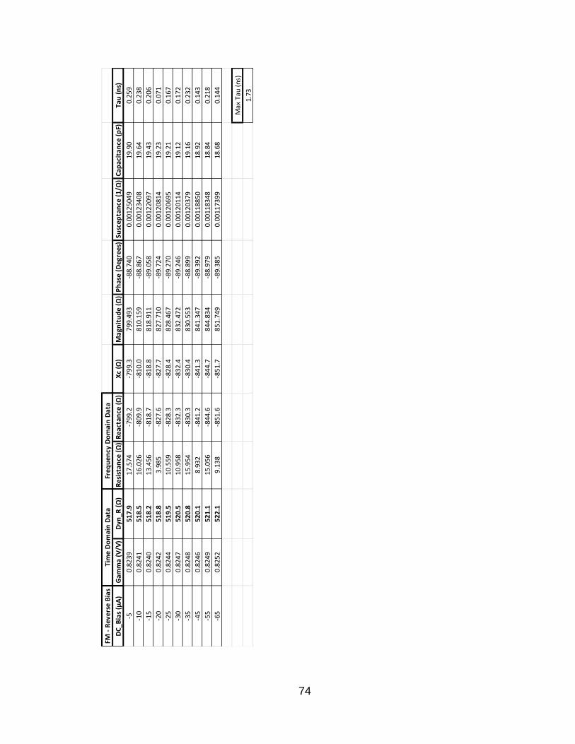
74

FM -

Rev

erse

Bia

s

DC_

Bia

s (μ

A)

Gam

ma

(V/V

)D

yn_R

(Ω

)R

esis

tan

ce (

Ω)

Rea

ctan

ce (

Ω)

Xc

(Ω)

Mag

nit

ud

e (Ω

)P

has

e (D

egre

es)

Susc

epta

nce

(1/

Ω)

Cap

acit

ance

(p

F)Ta

u (

ns)

-50.

8239

517.

917

.574

-799

.2-7

99.3

799.

493

-88.

740

0.00

1250

4919

.90

0.25

9

-10

0.82

4151

8.5

16.0

26-8

09.9

-810

.081

0.15

9-8

8.86

70.

0012

3408

19.6

40.

238

-15

0.82

4051

8.2

13.4

56-8

18.7

-818

.881

8.91

1-8

9.05

80.

0012

2097

19.4

30.

206

-20

0.82

4251

8.8

3.98

5-8

27.6

-827

.782

7.71

0-8

9.72

40.

0012

0814

19.2

30.

071

-25

0.82

4451

9.5

10.5

59-8

28.3

-828

.482

8.46

7-8

9.27

00.

0012

0695

19.2

10.

167

-30

0.82

4752

0.5

10.9

58-8

32.3

-832

.483

2.47

2-8

9.24

60.

0012

0114

19.1

20.

172

-35

0.82

4852

0.8

15.9

54-8

30.3

-830

.483

0.55

3-8

8.89

90.

0012

0379

19.1

60.

232

-45

0.82

4652

0.1

8.93

2-8

41.2

-841

.384

1.34

7-8

9.39

20.

0011

8850

18.9

20.

143

-55

0.82

4952

1.1

15.0

56-8

44.6

-844

.784

4.83

4-8

8.97

90.

0011

8348

18.8

40.

218

-65

0.82

5252

2.1

9.13

8-8

51.6

-851

.785

1.74

9-8

9.38

50.

0011

7399

18.6

80.

144

Max

Tau

(ns

)

1.73

Freq

uen

cy D

om

ain

Dat

aTi

me

Do

mai

n D

ata

75

BM

- F

orw

ard

Bia

s*

Lead

indu

ctan

ce e

stim

ated

to

be 0

.16

nH

bas

ed o

n hi

ghes

t re

acta

nce

mea

sure

men

t fr

om t

his

PUT.

DC_

Bia

s (m

A)

Gam

ma

(V/V

)D

yn_R

(Ω

)R

esis

tan

ce (

Ω)

Rea

ctan

ce (

Ω)

Xc

(Ω)

Mag

nit

ud

e (Ω

)P

has

e (D

egre

es)

Susc

epta

nce

(1/

Ω)

Cap

acit

ance

(p

F)Ta

u (

ns)

0.00

0.89

0986

6.6

45.4

57-7

45.6

00-7

45.6

1074

6.99

4-8

6.51

10.

0013

3622

21.2

70.

506

0.39

0.71

3729

9.3

322.

487

-425

.400

-425

.410

533.

827

-52.

836

0.00

1492

8223

.76

1.02

8

0.72

0.60

0020

0.0

293.

048

-224

.600

-224

.610

369.

225

-37.

469

0.00

1647

5926

.22

1.12

0

1.02

0.48

8914

5.7

237.

659

-136

.400

-136

.410

274.

025

-29.

855

0.00

1816

6328

.91

1.19

4

1.44

0.35

9210

6.1

180.

583

-81.

240

-81.

250

198.

020

-24.

224

0.00

2072

0832

.98

1.29

1

2.13

0.16

0069

.011

9.75

4-4

1.12

0-4

1.13

012

6.62

0-1

8.95

50.

0025

6538

40.8

31.

440

2.73

0.01

3651

.488

.637

-26.

090

-26.

100

92.4

00-1

6.40

80.

0030

5702

48.6

51.

555

3.43

-0.1

441

37.4

64.5

02-1

6.50

0-1

6.51

066

.581

-14.

357

0.00

3724

2759

.27

1.67

0

4.04

-0.2

755

28.4

49.4

27-1

1.49

0-1

1.50

050

.747

-13.

098

0.00

4465

5471

.07

1.76

7

5.74

-0.5

494

14.5

25.5

00-4

.595

-4.6

0525

.912

-10.

237

0.00

6858

2310

9.15

1.84

3

6.54

-0.6

500

10.6

18.9

62-3

.056

-3.0

6619

.208

-9.1

850.

0083

0989

132.

261.

818

8.04

-0.7

859

6.0

11.5

93-1

.504

-1.5

1411

.691

-7.4

400.

0110

7617

176.

281.

659

10.1

0-0

.873

23.

47.

891

-0.8

17-0

.827

7.93

4-5

.983

0.01

3137

0320

9.08

1.42

5

13.1

0-0

.923

42.

06.

083

-0.5

47-0

.557

6.10

8-5

.232

0.01

4927

7223

7.58

1.28

8

18.2

0-0

.963

90.

94.

801

-0.3

35-0

.345

4.81

3-4

.110

0.01

4890

8323

6.99

1.03

8

25.0

0-0

.991

40.

23.

970

-0.2

40-0

.250

3.97

8-3

.603

0.01

5799

3925

1.46

0.92

5

33.0

0-1

.000

00.

03.

407

-0.1

95-0

.205

3.41

3-3

.443

0.01

7597

0628

0.07

0.89

3

40.2

0-1

.000

00.

03.

065

-0.1

76-0

.186

3.07

1-3

.473

0.01

9726

7531

3.96

0.90

7

50.5

0-1

.000

00.

02.

753

-0.1

31-0

.141

2.75

7-2

.932

0.01

8555

3429

5.32

0.77

1

63.2

0-1

.000

00.

02.

386

-0.1

14-0

.124

2.38

9-2

.975

0.02

1722

4834

5.72

0.78

7

75.4

0-1

.000

00.

02.

194

-0.1

41-0

.151

2.19

9-3

.937

0.03

1221

3349

6.90

1.04

4

88.2

0-1

.000

00.

01.

967

-0.0

86-0

.096

1.96

9-2

.794

0.02

4753

0839

3.96

0.74

6

100.

00-1

.000

00.

01.

804

-0.1

09-0

.119

1.80

8-3

.774

0.03

6407

2857

9.44

1.00

9

115.

00-1

.000

00.

01.

620

-0.0

74-0

.084

1.62

2-2

.968

0.03

1921

4950

8.05

0.79

7

130.

00-1

.000

00.

01.

570

-0.0

86-0

.096

1.57

3-3

.499

0.03

8801

7461

7.55

0.94

0

Tim

e D

om

ain

Dat

aFr

equ

ency

Do

mai

n D

ata

76

BM

- R

ever

se B

ias

DC_

Bia

s (μ

A)

Gam

ma

(V/V

)D

yn_R

(Ω

)R

esis

tan

ce (

Ω)

Rea

ctan

ce (

Ω)

Xc

(Ω)

Mag

nit

ud

e (Ω

)P

has

e (D

egre

es)

Susc

epta

nce

(1/

Ω)

Cap

acit

ance

(p

F)Ta

u (

ns)

-50.

8528

629.

320

.362

-760

.3-7

60.3

760.

583

-88.

466

0.00

1314

3120

.92

0.30

3

-10

0.85

3063

0.3

15.8

46-7

81.3

-781

.378

1.47

1-8

8.83

80.

0012

7938

20.3

60.

245

-15

0.85

3363

1.7

21.2

13-7

80.7

-780

.778

0.99

8-8

8.44

40.

0012

7994

20.3

70.

303

-20

0.85

3263

1.2

11.4

00-7

92.6

-792

.679

2.69

2-8

9.17

60.

0012

6139

20.0

80.

186

-25

0.85

3263

1.2

21.5

31-7

98.9

-798

.979

9.20

0-8

8.45

60.

0012

5080

19.9

10.

300

-30

0.85

2762

8.9

14.2

56-8

01.9

-801

.980

2.03

7-8

8.98

20.

0012

4663

19.8

40.

220

-35

0.85

2862

9.3

8.11

2-8

11.3

-811

.381

1.35

1-8

9.42

70.

0012

3245

19.6

20.

137

-45

0.85

3263

1.2

17.6

57-8

13.5

-813

.581

3.70

2-8

8.75

70.

0012

2866

19.5

50.

255

-55

0.85

2962

9.8

18.8

30-8

33.9

-833

.983

4.12

3-8

8.70

60.

0011

9856

19.0

80.

261

Max

Tau

(ns

)

1.84

Tim

e D

om

ain

Dat

aFr

equ

ency

Do

mai

n D

ata

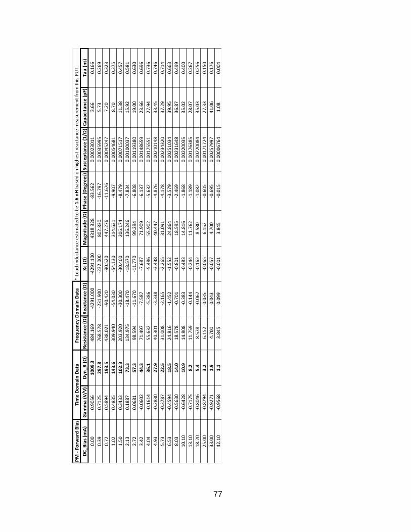
77

PM

- F

orw

ard

Bia

s*

Lea

d in

du

ctan

ce e

stim

ated

to

be

1.6

nH

bas

ed o

n h

igh

est

rea

ctan

ce m

easu

rem

ent

fro

m t

his

PU

T.

DC

_Bia

s (m

A)

Gam

ma

(V/V

)D

yn_R

(Ω

)R

esis

tan

ce (

Ω)

Rea

ctan

ce (

Ω)

Xc

(Ω)

Mag

nit

ud

e (

Ω)

Ph

ase

(D

egr

ee

s)Su

sce

pta

nce

(1

/Ω)

Cap

acit

ance

(p

F)Ta

u (

ns)

0.0

00

.90

56

10

09

.34

84

.16

9-4

29

1.0

00

-42

91

.10

04

31

8.3

28

-83

.56

20

.00

02

30

11

3.6

60

.16

6

0.3

90

.71

25

29

7.8

76

8.5

78

-23

1.9

00

-23

2.0

00

80

2.8

30

-16

.79

70

.00

03

59

95

5.7

30

.26

9

0.7

20

.58

94

19

3.5

43

8.0

21

-90

.42

0-9

0.5

20

44

7.2

76

-11

.67

60

.00

04

52

47

7.2

00

.32

3

1.0

20

.48

35

14

3.6

30

9.9

40

-54

.03

0-5

4.1

30

31

4.6

31

-9.9

07

0.0

00

54

68

18

.70

0.3

75

1.5

00

.34

33

10

2.3

20

3.9

20

-30

.30

0-3

0.4

00

20

6.1

74

-8.4

79

0.0

00

71

51

71

1.3

80

.45

7

2.1

30

.18

87

73

.31

34

.97

5-1

8.4

70

-18

.57

01

36

.24

6-7

.83

40

.00

10

00

37

15

.92

0.5

81

2.7

20

.06

81

57

.39

8.5

94

-11

.67

0-1

1.7

70

99

.29

4-6

.80

80

.00

11

93

80

19

.00

0.6

30

3.4

2-0

.06

02

44

.37

1.4

97

-7.5

87

-7.6

87

71

.90

9-6

.13

70

.00

14

86

59

23

.66

0.6

96

4.0

4-0

.16

14

36

.15

5.6

32

-5.3

86

-5.4

86

55

.90

2-5

.63

20

.00

17

55

51

27

.94

0.7

36

4.9

3-0

.28

30

27

.94

0.3

01

-3.3

38

-3.4

38

40

.44

7-4

.87

60

.00

21

01

48

33

.45

0.7

46

5.7

3-0

.37

87

22

.53

1.0

08

-2.1

65

-2.2

65

31

.09

1-4

.17

80

.00

23

43

20

37

.29

0.7

14

6.5

3-0

.45

94

18

.52

4.8

16

-1.4

52

-1.5

52

24

.86

4-3

.57

90

.00

25

10

34

39

.95

0.6

63

8.0

3-0

.56

30

14

.01

8.5

78

-0.7

01

-0.8

01

18

.59

5-2

.46

90

.00

23

16

48

36

.87

0.4

99

10

.10

-0.6

42

81

0.9

14

.80

8-0

.38

3-0

.48

31

4.8

16

-1.8

68

0.0

02

20

03

53

5.0

20

.40

0

13

.10

-0.7

17

58

.21

1.7

59

-0.1

44

-0.2

44

11

.76

2-1

.18

90

.00

17

63

85

28

.07

0.2

67

18

.20

-0.8

04

65

.48

.57

8-0

.06

2-0

.16

28

.58

0-1

.08

20

.00

22

00

84

35

.03

0.2

56

25

.00

-0.8

79

43

.26

.15

20

.03

5-0

.06

56

.15

2-0

.60

50

.00

17

17

24

27

.33

0.1

50

33

.00

-0.9

27

11

.94

.70

00

.04

3-0

.05

74

.70

0-0

.69

50

.00

25

79

97

41

.06

0.1

76

42

.10

-0.9

56

81

.13

.84

50

.09

9-0

.00

13

.84

5-0

.01

50

.00

00

67

64

1.0

80

.00

4

Tim

e D

om

ain

Dat

aFr

eq

ue

ncy

Do

mai

n D

ata

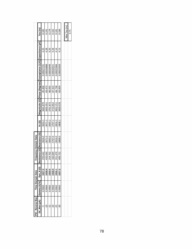
78

PM

- R

eve

rse

Bia

s

DC

_B

ias

(μA

)G

amm

a (V

/V)

Dyn

_R

(Ω

)R

esis

tan

ce (

Ω)

Rea

ctan

ce (

Ω)

Xc

(Ω)

Mag

nit

ud

e (

Ω)

Ph

ase

(D

egr

ee

s)Su

sce

pta

nce

(1/

Ω)

Cap

acit

ance

(p

F)Ta

u (

ns)

-50

.90

63

10

17

.22

93

.64

2-3

65

4.0

-36

54

.13

66

5.8

79

-85

.40

60

.00

02

71

91

4.3

30

.18

5

-10

0.9

06

41

01

8.4

42

0.0

30

-36

71

.0-3

67

1.1

36

95

.05

1-8

3.4

73

0.0

00

26

88

84

.28

0.1

91

-15

0.9

06

51

01

9.5

25

4.7

02

-36

93

.0-3

69

3.1

37

01

.87

3-8

6.0

55

0.0

00

26

94

94

.29

0.1

79

-20

0.9

06

41

01

8.4

16

6.8

39

-37

07

.0-3

70

7.1

37

10

.85

2-8

7.4

23

0.0

00

26

92

14

.28

0.1

65

-25

0.9

06

21

01

6.1

35

1.4

70

-38

16

.0-3

81

6.1

38

32

.25

1-8

4.7

38

0.0

00

25

98

44

.14

0.1

81

-30

0.9

06

31

01

7.2

40

9.7

22

-38

08

.0-3

80

8.1

38

30

.07

8-8

3.8

59

0.0

00

25

95

94

.13

0.1

84

Max

Tau

(n

s)

0.7

5

Tim

e D

om

ain

Dat

aFr

eq

ue

ncy

Do

mai

n D

ata

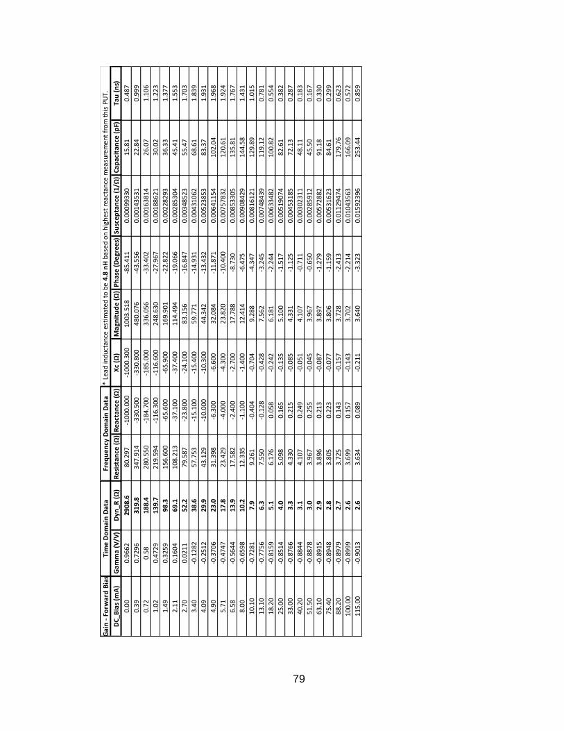
79

Gai

n -

Fo

rwar

d B

ias

* Le

ad in

duct

ance

est

imat

ed t

o be

4.8

nH

bas

ed o

n hi

ghes

t re

acta

nce

mea

sure

men

t fr

om t

his

PUT.

DC_

Bia

s (m

A)

Gam

ma

(V/V

)D

yn_R

(Ω

)R

esis

tan

ce (

Ω)

Rea

ctan

ce (

Ω)

Xc

(Ω)

Mag

nit

ud

e (Ω

)P

has

e (D

egre

es)

Susc

epta

nce

(1/

Ω)

Cap

acit

ance

(p

F)Ta

u (

ns)

0.00

0.96

6229

08.6

80.2

97-1

000.

000

-100

0.30

010

03.5

18-8

5.41

10.

0009

9330

15.8

10.

487

0.39

0.72

9631

9.8

347.

914

-330

.500

-330

.800

480.

076

-43.

556

0.00

1435

3122

.84

0.99

9

0.72

0.58

188.

428

0.55

0-1

84.7

00-1

85.0

0033

6.05

6-3

3.40

20.

0016

3814

26.0

71.

106

1.02

0.47

2913

9.7

219.

594

-116

.300

-116

.600

248.

630

-27.

967

0.00

1886

2130

.02

1.22

3

1.49

0.32

5998

.315

6.60

0-6

5.60

0-6

5.90

016

9.90

1-2

2.82

20.

0022

8293

36.3

31.

377

2.11

0.16

0469

.110

8.21

3-3

7.10

0-3

7.40

011

4.49

4-1

9.06

60.

0028

5304

45.4

11.

553

2.70

0.02

1152

.279

.587

-23.

800

-24.

100

83.1

56-1

6.84

70.

0034

8523

55.4

71.

703

3.40

-0.1

282

38.6

57.7

53-1

5.10

0-1

5.40

059

.771

-14.

931

0.00

4310

6268

.61

1.83

9

4.09

-0.2

512

29.9

43.1

29-1

0.00

0-1

0.30

044

.342

-13.

432

0.00

5238

5383

.37

1.93

1

4.90

-0.3

706

23.0

31.3

98-6

.300

-6.6

0032

.084

-11.

871

0.00

6411

5410

2.04

1.96

8

5.71

-0.4

747

17.8

23.4

29-4

.000

-4.3

0023

.820

-10.

400

0.00

7578

3212

0.61

1.92

4

6.58

-0.5

644

13.9

17.5

82-2

.400

-2.7

0017

.788

-8.7

300.

0085

3305

135.

811.

767

8.00

-0.6

598

10.2

12.3

35-1

.100

-1.4

0012

.414

-6.4

750.

0090

8429

144.

581.

431

10.1

0-0

.728

17.

99.

261

-0.4

04-0

.704

9.28

8-4

.347

0.00

8161

2112

9.89

1.01

5

13.1

0-0

.775

66.

37.

550

-0.1

28-0

.428

7.56

2-3

.245

0.00

7484

3911

9.12

0.78

1

18.2

0-0

.815

95.

16.

176

0.05

8-0

.242

6.18

1-2

.244

0.00

6334

8210

0.82

0.55

4

25.0

0-0

.851

44.

05.

098

0.16

5-0

.135

5.10

0-1

.517

0.00

5190

7482

.61

0.38

2

33.0

0-0

.876

63.

34.

330

0.21

5-0

.085

4.33

1-1

.125

0.00

4531

8572

.13

0.28

7

40.2

0-0

.884

43.

14.

107

0.24

9-0

.051

4.10

7-0

.711

0.00

3023

1148

.11

0.18

3

51.5

0-0

.887

83.

03.

967

0.25

5-0

.045

3.96

7-0

.650

0.00

2859

1245

.50

0.16

7

63.1

0-0

.891

52.

93.

896

0.21

3-0

.087

3.89

7-1

.279

0.00

5728

8291

.18

0.33

0

75.4

0-0

.894

82.

83.

805

0.22

3-0

.077

3.80

6-1

.159

0.00

5316

2384

.61

0.29

9

88.2

0-0

.897

92.

73.

725

0.14

3-0

.157

3.72

8-2

.413

0.01

1294

7417

9.76

0.62

3

100.

00-0

.899

92.

63.

699

0.15

7-0

.143

3.70

2-2

.214

0.01

0435

6316

6.09

0.57

2

115.

00-0

.901

32.

63.

634

0.08

9-0

.211

3.64

0-3

.323

0.01

5923

9625

3.44

0.85

9

Tim

e D

om

ain

Dat

aFr

equ

ency

Do

mai

n D

ata

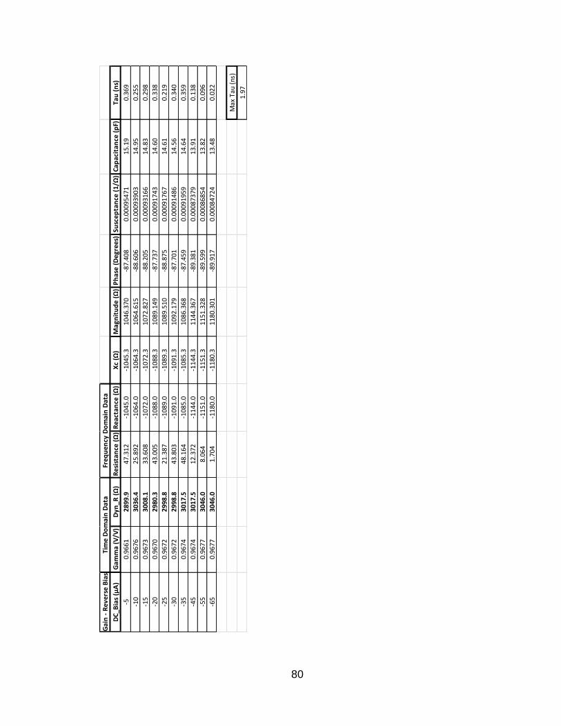
80

Gai

n -

Rev

ers

e B

ias

DC

_Bia

s (μ

A)

Gam

ma

(V/V

)D

yn_R

(Ω

)R

esis

tan

ce (

Ω)

Rea

ctan

ce (

Ω)

Xc

(Ω)

Mag

nit

ud

e (

Ω)

Ph

ase

(D

egr

ee

s)Su

sce

pta

nce

(1

/Ω)

Cap

acit

ance

(p

F)Ta

u (

ns)

-50

.96

61

28

99

.94

7.3

12

-10

45

.0-1

04

5.3

10

46

.37

0-8

7.4

08

0.0

00

95

47

11

5.1

90

.36

9

-10

0.9

67

63

03

6.4

25

.89

2-1

06

4.0

-10

64

.31

06

4.6

15

-88

.60

60

.00

09

39

03

14

.95

0.2

55

-15

0.9

67

33

00

8.1

33

.60

8-1

07

2.0

-10

72

.31

07

2.8

27

-88

.20

50

.00

09

31

66

14

.83

0.2

98

-20

0.9

67

02

98

0.3

43

.00

5-1

08

8.0

-10

88

.31

08

9.1

49

-87

.73

70

.00

09

17

43

14

.60

0.3

38

-25

0.9

67

22

99

8.8

21

.38

7-1

08

9.0

-10

89

.31

08

9.5

10

-88

.87

50

.00

09

17

67

14

.61

0.2

19

-30

0.9

67

22

99

8.8

43

.80

3-1

09

1.0

-10

91

.31

09

2.1

79

-87

.70

10

.00

09

14

86

14

.56

0.3

40

-35

0.9

67

43

01

7.5

48

.16

4-1

08

5.0

-10

85

.31

08

6.3

68

-87

.45

90

.00

09

19

59

14

.64

0.3

59

-45

0.9

67

43

01

7.5

12

.37

2-1

14

4.0

-11

44

.31

14

4.3

67

-89

.38

10

.00

08

73

79

13

.91

0.1

38

-55

0.9

67

73

04

6.0

8.0

64

-11

51

.0-1

15

1.3

11

51

.32

8-8

9.5

99

0.0

00

86

85

41

3.8

20

.09

6

-65

0.9

67

73

04

6.0

1.7

04

-11

80

.0-1

18

0.3

11

80

.30

1-8

9.9

17

0.0

00

84

72

41

3.4

80

.02

2

Max

Tau

(n

s)

1.9

7

Tim

e D

om

ain

Dat

aFr

eq

ue

ncy

Do

mai

n D

ata

81

SOA

- F

orw

ard

Bia

s*

Lead

indu

ctan

ce e

stim

ated

to

be 1

6 n

H b

ased

on

high

est

reac

tanc

e m

easu

rem

ent

from

thi

s PU

T.

DC_

Bia

s (m

A)

Gam

ma

(V/V

)D

yn_R

(Ω

)R

esis

tan

ce (

Ω)

Rea

ctan

ce (

Ω)

Xc

(Ω)

Mag

nit

ud

e (Ω

)P

has

e (D

egre

es)

Susc

epta

nce

(1/

Ω)

Cap

acit

ance

(p

F)Ta

u (

ns)

0.00

0.88

1179

1.0

122.

652

-136

7.00

0-1

367.

100

1372

.591

-84.

873

0.00

0725

6311

.55

0.41

0.39

0.60

8220

5.2

431.

538

-367

.100

-367

.200

566.

622

-40.

395

0.00

1143

7118

.20

0.82

0.72

0.47

8414

1.7

310.

438

-175

.900

-176

.000

356.

858

-29.

551

0.00

1382

0422

.00

0.95

1.02

0.36

4310

7.3

236.

271

-107

.900

-108

.000

259.

784

-24.

565

0.00

1600

2825

.47

1.05

1.43

0.23

5480

.817

2.39

8-6

5.89

0-6

5.99

018

4.59

6-2

0.94

60.

0019

3657

30.8

21.

19

2.13

0.04

4054

.611

1.37

8-3

4.58

0-3

4.68

011

6.65

2-1

7.29

50.

0025

4855

40.5

61.

40

2.72

-0.0

957

41.3

81.5

52-2

2.63

0-2

2.73

084

.660

-15.

574

0.00

3171

3150

.47

1.56

3.42

-0.2

419

30.5

59.0

51-1

4.61

0-1

4.71

060

.856

-13.

988

0.00

3972

0263

.22

1.71

4.04

-0.3

526

23.9

45.3

37-1

0.28

0-1

0.38

046

.510

-12.

896

0.00

4798

4776

.37

1.82

4.92

-0.4

781

17.7

31.9

33-6

.307

-6.4

0732

.569

-11.

345

0.00

6039

9796

.13

1.87

5.73

-0.5

745

13.5

23.7

33-4

.076

-4.1

7624

.098

-9.9

790.

0071

9139

114.

451.

84

6.53

-0.6

505

10.6

18.2

83-2

.665

-2.7

6518

.491

-8.6

000.

0080

8685

128.

711.

72

8.03

-0.7

403

7.5

12.5

04-1

.280

-1.3

8012

.580

-6.2

980.

0087

2014

138.

791.

39

10.1

0-0

.803

85.

49.

478

-0.6

07-0

.707

9.50

4-4

.266

0.00

7826

6512

4.57

0.99

13.1

0-0

.847

74.

17.

760

-0.2

96-0

.396

7.77

0-2

.921

0.00

6559

0710

4.39

0.70

18.2

0-0

.885

13.

06.

454

-0.1

48-0

.248

6.45

9-2

.201

0.00

5945

0294

.62

0.54

25.0

0-0

.911

02.

35.

631

-0.0

85-0

.185

5.63

4-1

.882

0.00

5828

1792

.76

0.47

33.0

0-0

.929

61.

85.

013

0.00

7-0

.093

5.01

4-1

.063

0.00

3699

4658

.88

0.27

40.2

0-0

.940

21.

54.

685

-0.0

22-0

.122

4.68

7-1

.492

0.00

5554

5288

.40

0.38

51.5

0-0

.955

21.

14.

255

0.03

7-0

.063

4.25

5-0

.848

0.00

3478

9355

.37

0.22

63.2

0-0

.966

80.

83.

946

0.06

0-0

.040

3.94

6-0

.581

0.00

2568

6340

.88

0.15

75.4

0-0

.977

10.

63.

694

-0.0

03-0

.103

3.69

5-1

.597

0.00

7542

3412

0.04

0.41

88.2

0-0

.984

40.

43.

432

0.01

7-0

.083

3.43

3-1

.385

0.00

7042

5411

2.09

0.36

100.

00-0

.991

10.

23.

268

0.02

1-0

.079

3.26

9-1

.385

0.00

7392

8111

7.66

0.36

115.

00-0

.997

10.

13.

046

0.02

3-0

.077

3.04

7-1

.448

0.00

8293

8013

2.00

0.38

130.

00-1

.000

00.

02.

960

0.00

4-0

.096

2.96

2-1

.858

0.01

0945

3917

4.20

0.49

145.

00-1

.000

00.

02.

845

-0.0

36-0

.136

2.84

8-2

.737

0.01

6764

2126

6.81

0.72

160.

00-1

.000

00.

02.

710

-0.0

54-0

.154

2.71

4-3

.252

0.02

0901

7233

2.66

0.86

Tim

e D

om

ain

Dat

aFr

equ

ency

Do

mai

n D

ata

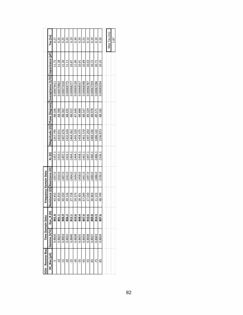
82

SOA

- R

eve

rse

Bia

s

DC

_Bia

s (μ

A)

Gam

ma

(V/V

)D

yn_R

(Ω

)R

esis

tan

ce (

Ω)

Rea

ctan

ce (

Ω)

Xc

(Ω)

Mag

nit

ud

e (

Ω)

Ph

ase

(D

egr

ee

s)Su

sce

pta

nce

(1

/Ω)

Cap

acit

ance

(p

F)Ta

u (

ns)

-50

.88

26

80

1.8

43

.45

2-1

35

7.0

-13

57

.11

35

7.7

95

-88

.16

60

.00

07

36

11

11

.72

0.2

7

-10

0.8

82

58

01

.13

9.4

33

-14

10

.0-1

41

0.1

14

10

.65

1-8

8.3

98

0.0

00

70

86

21

1.2

80

.25

-15

0.8

83

38

06

.94

0.2

50

-14

07

.0-1

40

7.1

14

07

.67

6-8

8.3

62

0.0

00

71

01

01

1.3

00

.25

-20

0.8

83

28

06

.23

9.1

16

-14

32

.0-1

43

2.1

14

32

.63

4-8

8.4

35

0.0

00

69

77

51

1.1

10

.24

-25

0.8

84

08

12

.12

7.7

18

-14

64

.0-1

46

4.1

14

64

.36

2-8

8.9

15

0.0

00

68

27

71

0.8

70

.19

-30

0.8

83

88

10

.65

9.3

74

-14

44

.0-1

44

4.1

14

45

.32

0-8

7.6

46

0.0

00

69

13

01

1.0

00

.30

-35

0.8

83

58

08

.42

8.3

01

-14

58

.0-1

45

8.1

14

58

.37

5-8

8.8

88

0.0

00

68

55

71

0.9

10

.20

-45

0.8

83

48

07

.63

7.0

49

-14

61

.0-1

46

1.1

14

61

.57

0-8

8.5

47

0.0

00

68

39

81

0.8

90

.23

-55

0.8

83

88

10

.61

7.5

30

-14

97

.0-1

49

7.1

14

97

.20

3-8

9.3

29

0.0

00

66

78

71

0.6

30

.14

-65

0.8

83

78

09

.82

6.4

63

-14

84

.0-1

48

4.1

14

84

.33

6-8

8.9

78

0.0

00

67

35

91

0.7

20

.19

-75

0.8

84

38

14

.31

1.1

15

-14

86

.0-1

48

6.1

14

86

.14

2-8

9.5

71

0.0

00

67

28

61

0.7

10

.10

-85

0.8

83

48

07

.64

8.7

49

-15

36

.0-1

53

6.1

15

36

.87

3-8

8.1

82

0.0

00

65

03

41

0.3

50

.26

Max

Tau

(n

s)

1.8

7

Tim

e D

om

ain

Dat

aFr

eq

ue

ncy

Do

mai

n D

ata

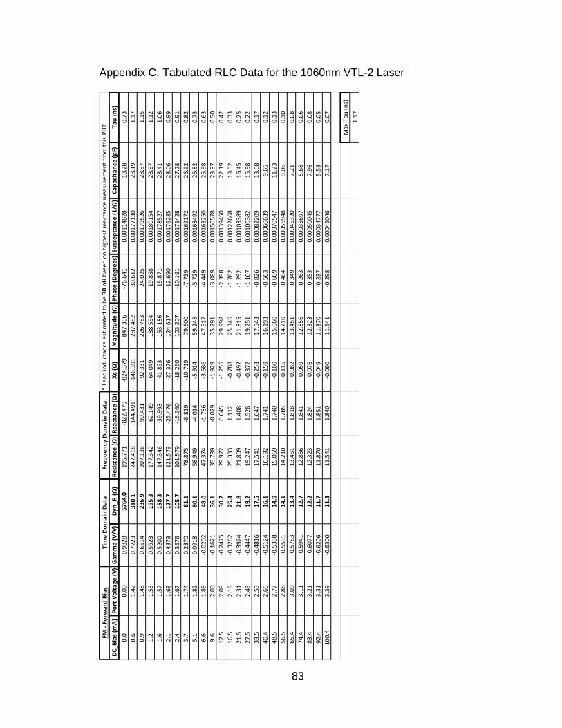
83

Appendix C: Tabulated RLC Data for the 1060nm VTL-2 Laser

* Le

ad in

duct

ance

est

imat

ed t

o be

30

nH

bas

ed o

n hi

ghes

t re

acta

nce

mea

sure

men

t fr

om t

his

PUT.

DC_

Bia

s (m

A)

Po

rt V

olt

age

(V)

Gam

ma

(V/V

)D

yn_R

(Ω

)R

esis

tan

ce (

Ω)

Rea

ctan

ce (

Ω)

Xc

(Ω)

Mag

nit

ud

e (Ω

)P

has

e (D

egre

es)

Susc

epta

nce

(1/

Ω)

Cap

acit

ance

(p

F)Ta

u (

ns)

0.0

0.00

0.98

2857

64.0

195.

771

-822

.479

-824

.379

847.

306

-76.

641

0.00

1148

2818

.28

0.73

0.6

1.42

0.72

2331

0.1

247.

418

-144

.491

-146

.391

287.

482

-30.

612

0.00

1771

3028

.19

1.17

0.9

1.48

0.65

1423

6.9

207.

136

-90.

431

-92.

331

226.

783

-24.

025

0.00

1795

2628

.57

1.15

1.2

1.53

0.59

2319

5.3

177.

342

-62.

149

-64.

049

188.

554

-19.

858

0.00

1801

5428

.67

1.12

1.6

1.57

0.52

0015

8.3

147.

346

-39.

993

-41.

893

153.

186

-15.

871

0.00

1785

2728

.41

1.06

2.1

1.63

0.43

7312

7.7

121.

573

-25.

476

-27.

376

124.

617

-12.

690

0.00

1762

8528

.06

0.99

2.4

1.67

0.35

7610

5.7

101.

579

-16.

360

-18.

260

103.

207

-10.

191

0.00

1714

2827

.28

0.91

3.7

1.74

0.23

7081

.178

.875

-8.8

19-1

0.71

979

.600

-7.7

390.

0016

9172

26.9

20.

82

5.1

1.82

0.09

1860

.158

.949

-4.0

14-5

.914

59.2

45-5

.729

0.00

1684

9226

.82

0.73

6.6

1.89

-0.0

202

48.0

47.3

74-1

.786

-3.6

8647

.517

-4.4

490.

0016

3250

25.9

80.

63

9.6

2.00

-0.1

621

36.1

35.7

39-0

.029

-1.9

2935

.791

-3.0

890.

0015

0578

23.9

70.

50

12.5

2.09

-0.2

475

30.2

29.9

720.

645

-1.2

5529

.998

-2.3

980.

0013

9450

22.1

90.

42

16.5

2.19

-0.3

262

25.4

25.3

331.

112

-0.7

8825

.345

-1.7

820.

0012

2668

19.5

20.

33

21.5

2.31

-0.3

924

21.8

21.8

091.

408

-0.4

9221

.815

-1.2

920.

0010

3389

16.4

50.

25

27.5

2.43

-0.4

447

19.2

19.2

471.

528

-0.3

7219

.251

-1.1

070.

0010

0382

15.9

80.

22

33.5

2.53

-0.4

816

17.5

17.5

411.

647

-0.2

5317

.543

-0.8

260.

0008

2209

13.0

80.

17

40.4

2.65

-0.5

124

16.1

16.1

921.

741

-0.1

5916

.193

-0.5

630.

0006

0639

9.65

0.12

48.5

2.77

-0.5

398

14.9

15.0

591.

740

-0.1

6015

.060

-0.6

090.

0007

0547

11.2

30.

13

56.5

2.88

-0.5

591

14.1

14.2

101.

785

-0.1

1514

.210

-0.4

640.

0005

6948

9.06

0.10

65.4

3.00

-0.5

783

13.4

13.4

511.

818

-0.0

8213

.451

-0.3

490.

0004

5320

7.21

0.08

74.4

3.11

-0.5

941

12.7

12.8

561.

841

-0.0

5912

.856

-0.2

630.

0003

5697

5.68

0.06

83.4

3.21

-0.6

077

12.2

12.3

231.

824

-0.0

7612

.323

-0.3

530.

0005

0045

7.96

0.08

92.4

3.31

-0.6

206

11.7

11.8

701.

851

-0.0

4911

.870

-0.2

370.

0003

4777

5.53

0.05

100.

43.

39-0

.630

011

.311

.541

1.84

0-0

.060

11.5

41-0

.298

0.00

0450

467.

170.

07

Max

Tau

(ns

)

1.17

Tim

e D

om

ain

Dat

aFM

- F

orw

ard

Bia

sFr

equ

ency

Do

mai

n D

ata

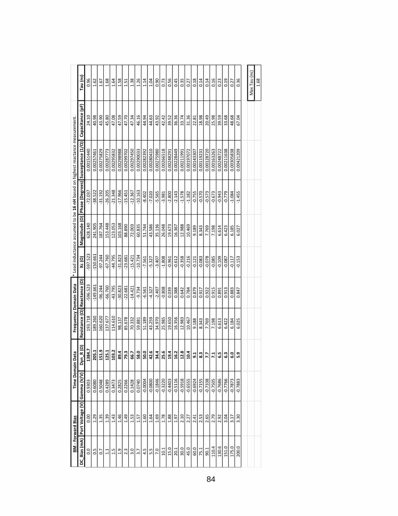
84

* Le

ad in

duct

ance

ass

umed

to

be 1

6 n

H b

ased

on

high

est

reac

tanc

e m

easu

rem

ent.

DC_

Bia

s (m

A)

Po

rt V

olt

age

(V)

Gam

ma

(V/V

)D

yn_R

(Ω

)R

esis

tan

ce (

Ω)

Rea

ctan

ce (

Ω)

Xc

(Ω)

Mag

nit

ud

e (Ω

)P

has

e (D

egre

es)

Susc

epta

nce

(1/

Ω)

Cap

acit

ance

(p

F)Ta

u (

ns)

0.0

0.00

0.93

0313

84.7

193.

718

-596

.523

-597

.523

628.

140

-72.

037

0.00

1514

4024

.10

0.96

0.5

1.29

0.60

8020

5.1

189.

260

-149

.661

-150

.661

241.

905

-38.

522

0.00

2574

6140

.98

1.62

0.7

1.35

0.50

4815

1.9

160.

620

-96.

244

-97.

244

187.

764

-31.

192

0.00

2758

2943

.90

1.67

1.1

1.39

0.42

8912

5.1

137.

677

-66.

760

-67.

760

153.

448

-26.

205

0.00

2877

7345

.80

1.68

1.5

1.43

0.34

7310

3.2

114.

610

-43.

795

-44.

795

123.

053

-21.

348

0.00

2958

3247

.08

1.64

1.9

1.46

0.28

2589

.498

.137

-30.

823

-31.

823

103.

168

-17.

966

0.00

2989

8847

.59

1.58

2.3

1.49

0.22

6679

.385

.678

-22.

681

-23.

681

88.8

90-1

5.45

10.

0029

9702

47.7

01.

51

3.0

1.53

0.14

2866

.770

.332

-14.

421

-15.

421

72.0

03-1

2.36

70.

0029

7450

47.3

41.

38

3.7

1.57

0.07

4058

.059

.881

-9.7

34-1

0.73

460

.835

-10.

163

0.00

2900

3346

.16

1.26

4.5

1.60

-0.0

004

50.0

51.1

89-6

.561

-7.5

6151

.744

-8.4

020.

0028

2392

44.9

41.

14

5.5

1.64

-0.0

800

42.6

43.2

59-4

.327

-5.3

2743

.586

-7.0

200.

0028

0410

44.6

31.

04

7.0

1.69

-0.1

846

34.4

34.9

70-2

.407

-3.4

0735

.136

-5.5

650.

0027

5980

43.9

20.

90

10.1

1.78

-0.3

220

25.6

25.9

85-0

.808

-1.8

0826

.048

-3.9

810.

0026

6518

42.4

20.

73

15.0

1.88

-0.4

403

19.4

19.6

500.

039

-0.9

6119

.673

-2.8

000.

0024

8291

39.5

20.

56

20.1

1.97

-0.5

116

16.2

16.3

560.

388

-0.6

1216

.367

-2.1

430.

0022

8449

36.3

60.

45

30.0

2.10

-0.5

918

12.8

12.9

830.

642

-0.3

5812

.988

-1.5

780.

0021

1991

33.7

40.

35

45.0

2.27

-0.6

555

10.4

10.4

670.

784

-0.2

1610

.469

-1.1

820.

0019

7072

31.3

60.

27

60.0

2.41

-0.6

924

9.1

9.18

80.

879

-0.1

219.

189

-0.7

550.

0014

3307

22.8

10.

18

75.1

2.53

-0.7

155

8.3

8.34

30.

917

-0.0

838.

343

-0.5

700.

0011

9231

18.9

80.

14

90.1

2.65

-0.7

338

7.7

7.76

90.

922

-0.0

787.

769

-0.5

730.

0012

8720

20.4

90.

14

110.

42.

79-0

.750

57.

17.

198

0.91

5-0

.085

7.19

8-0

.673

0.00

1632

6325

.98

0.16

130.

62.

92-0

.768

66.

56.

613

0.89

1-0

.109

6.61

4-0

.943

0.00

2487

2239

.59

0.23

151.

03.

04-0

.776

66.

36.

422

0.91

3-0

.087

6.42

3-0

.779

0.00

2116

3833

.68

0.19

175.

03.

17-0

.787

36.

06.

184

0.88

3-0

.117

6.18

5-1

.084

0.00

3058

3848

.68

0.27

200.

03.

30-0

.788

35.

96.

025

0.84

7-0

.153

6.02

7-1

.455

0.00

4212

0967

.04

0.36

Max

Tau

(ns

)

1.68

Tim

e D

om

ain

Dat

aB

M -

Fo

rwar

d B

ias

Freq

uen

cy D

om

ain

Dat

a

85

* Le

ad in

duct

ance

ass

umed

to

be 2

9 n

H b

ased

on

high

est

reac

tanc

e m

easu

rem

ent.

DC_

Bia

s (m

A)

Po

rt V

olt

age

(V)

Gam

ma

(V/V

)D

yn_R

(Ω

)R

esis

tan

ce (

Ω)

Rea

ctan

ce (

Ω)

Rea

ctan

ce (

Ω)

Mag

nit

ud

e (Ω

)P

has

e (D

egre

es)

Susc

epta

nce

(1/

Ω)

Cap

acit

ance

(p

F)Ta

u (

ns)

0.0

0.00

0.97

9949

25.1

138.

235

-651

.523

-653

.323

667.

787

-78.

053

0.00

1465

0523

.32

0.86

0.6

1.35

0.66

2324

6.1

188.

146

-133

.414

-135

.214

231.

693

-35.

703

0.00

2518

8140

.09

1.58

0.9

1.40

0.57

8018

7.0

159.

442

-85.

322

-87.

122

181.

692

-28.

653

0.00

2639

1042

.00

1.60

1.3

1.45

0.48

7014

4.9

132.

260

-53.

862

-55.

662

143.

496

-22.

824

0.00

2703

2243

.02

1.56

1.8

1.49

0.39

4411

5.1

108.

990

-34.

145

-35.

945

114.

764

-18.

253

0.00

2729

1343

.44

1.49

2.4

1.54

0.29

2191

.388

.108

-20.

576

-22.

376

90.9

05-1

4.25

00.

0027

0774

43.1

01.

37

3.4

1.60

0.16

1269

.267

.663

-10.

469

-12.

269

68.7

66-1

0.27

70.

0025

9452

41.2

91.

19

4.8

1.66

0.01

6251

.651

.160

-4.9

05-6

.705

51.5

98-7

.467

0.00

2518

5040

.08

1.01

6.3

1.72

-0.1

022

40.7

40.3

23-2

.273

-4.0

7340

.528

-5.7

680.

0024

7971

39.4

70.

88

9.3

1.81

-0.2

601

29.4

29.3

94-0

.224

-2.0

2429

.464

-3.9

390.

0023

3152

37.1

10.

69

12.2

1.88

-0.3

516

24.0

24.1

440.

550

-1.2

5024

.176

-2.9

630.

0021

3809

34.0

30.

55

16.2

1.96

-0.4

305

19.9

20.0

940.

989

-0.8

1120

.110

-2.3

120.

0020

0629

31.9

30.

46

21.3

2.05

-0.4

943

16.9

17.1

321.

256

-0.5

4417

.141

-1.8

190.

0018

5159

29.4

70.

38

27.3

2.14

-0.5

451

14.7

14.9

951.

439

-0.3

6114

.999

-1.3

790.

0016

0458

25.5

40.

29

33.3

2.23

-0.5

804

13.3

13.5

891.

576

-0.2

2413

.591

-0.9

440.

0012

1270

19.3

00.

21

40.2

2.32

-0.6

083

12.2

12.4

431.

632

-0.1

6812

.444

-0.7

740.

0010

8488

17.2

70.

17

48.2

2.41

-0.6

324

11.3

11.5

931.

696

-0.1

0411

.593

-0.5

140.

0007

7376

12.3

10.

12

56.2

2.50

-0.6

441

10.8

10.9

201.

724

-0.0

7610

.920

-0.3

990.

0006

3730

10.1

40.

09

65.2

2.61

-0.6

625

10.2

10.4

941.

724

-0.0

7610

.494

-0.4

150.

0006

9009

10.9

80.

10

74.2

2.70

-0.6

733

9.8

9.95

41.

741

-0.0

599.

954

-0.3

400.

0005

9544

9.48

0.08

83.2

2.79

-0.6

856

9.3

9.59

61.

790

-0.0

109.

596

-0.0

600.

0001

0860

1.73

0.01

92.2

2.87

-0.6

933

9.1

9.26

81.

763

-0.0

379.

268

-0.2

290.

0004

3075

6.86

0.05

100.

22.

94-0

.701

28.

89.

056

1.76

4-0

.036

9.05

6-0

.228

0.00

0438

966.

990.

05

Max

Tau

(ns

)

1.60

Tim

e D

om

ain

Dat

aP

M -

Fo

rwar

d B

ias

Freq

uen

cy D

om

ain

Dat

a

86

* Le

ad in

duct

ance

ass

umed

to

be 3

0 n

H b

ased

on

high

est

reac

tanc

e m

easu

rem

ent.

DC_

Bia

s (m

A)

Po

rt V

olt

age

(V)

Gam

ma

(V/V

)D

yn_R

(Ω

)R

esis

tan

ce (

Ω)

Rea

ctan

ce (

Ω)

Xc

(Ω)

Mag

nit

ud

e (Ω

)P

has

e (D

egre

es)

Susc

epta

nce

(1/

Ω)

Cap

acit

ance

(p

F)Ta

u (

ns)

0.0

0.00

0.93

8215

68.1

83.8

60-2

79.7

54-2

81.6

5429

3.87

3-7

3.42

00.

0032

6134

51.9

11.

63

0.3

1.02

0.79

2143

1.0

124.

110

-178

.449

-180

.349

218.

927

-55.

466

0.00

3762

8359

.89

2.13

0.6

1.06

0.71

2229

7.5

127.

638

-137

.247

-139

.147

188.

821

-47.

470

0.00

3902

7862

.11

2.23

0.9

1.09

0.63

1922

1.7

122.

409

-103

.932

-105

.832

161.

816

-40.

846

0.00

4041

8064

.33

2.28

1.2

1.11

0.55

8917

6.7

114.

197

-80.

994

-82.

894

141.

111

-35.

975

0.00

4162

9466

.26

2.30

1.5

1.13

0.49

1114

6.5

104.

703

-63.

340

-65.

240

123.

365

-31.

927

0.00

4286

7568

.23

2.31

1.8

1.15

0.42

2612

3.2

95.4

75-5

0.05

3-5

1.95

310

8.69

5-2

8.55

30.

0043

9736

69.9

92.

30

2.1

1.16

0.35

0210

3.9

85.6

22-3

8.93

4-4

0.83

494

.861

-25.

497

0.00

4537

8572

.22

2.28

3.1

1.20

0.15

0967

.862

.654

-19.

257

-21.

157

66.1

30-1

8.65

90.

0048

3794

77.0

02.

14

4.1

1.23

-0.0

208

48.0

46.5

18-9

.747

-11.

647

47.9

54-1

4.05

70.

0050

6484

80.6

11.

94

5.1

1.26

-0.1

442

37.4

35.7

22-4

.815

-6.7

1536

.348

-10.

646

0.00

5082

6880

.89

1.69

6.1

1.29

-0.2

609

29.3

28.4

48-2

.145

-4.0

4528

.734

-8.0

930.

0048

9917

77.9

71.

41

7.1

1.31

-0.3

435

24.4

23.9

33-0

.763

-2.6

6324

.081

-6.3

500.

0045

9263

73.0

91.

18

10.3

1.36

-0.5

028

16.5

16.4

73-0

.841

-2.7

4116

.700

-9.4

480.

0098

2955

156.

441.

94

15.3

1.42

-0.6

349

11.2

11.2

921.

524

-0.3

7611

.298

-1.9

070.

0029

4554

46.8

80.

43

20.3

1.47

-0.6

878

9.2

9.32

01.

726

-0.1

749.

322

-1.0

700.

0020

0247

31.8

70.

25

30.2

1.55

-0.7

412

7.4

7.46

11.

782

-0.1

187.

462

-0.9

060.

0021

1924

33.7

30.

22

40.2

1.61

-0.7

745

6.4

6.45

31.

807

-0.0

936.

454

-0.8

260.

0022

3290

35.5

40.

20

55.2

1.70

-0.8

030

5.5

5.54

91.

833

-0.0

675.

549

-0.6

920.

0021

7561

34.6

30.

17

70.2

1.78

-0.8

190

5.0

4.99

31.

793

-0.1

074.

994

-1.2

280.

0042

9004

68.2

80.

31

85.2

1.84

-0.8

330

4.6

4.61

31.

809

-0.0

914.

614

-1.1

300.

0042

7470

68.0

30.

29

105.

21.

93-0

.847

04.

14.

265

1.83

4-0

.066

4.26

6-0

.887

0.00

3627

4557

.73

0.23

125.

22.

00-0

.854

13.

93.

979

1.84

8-0

.052

3.97

9-0

.749

0.00

3283

8352

.26

0.19

145.

22.

07-0

.860

13.

83.

832

1.86

6-0

.034

3.83

2-0

.508

0.00

2315

2336

.85

0.13

165.

12.

14-0

.864

73.

63.

704

1.81

2-0

.088

3.70

5-1

.361

0.00

6410

5610

2.03

0.35

195.

12.

23-0

.868

03.

53.

542

1.80

9-0

.091

3.54

3-1

.472

0.00

7248

6611

5.37

0.38

225.

12.

32-0

.871

03.

43.

483

1.77

7-0

.123

3.48

5-2

.023

0.01

0126

4416

1.17

0.52

255.

12.

41-0

.872

43.

43.

481

1.69

0-0

.210

3.48

7-3

.452

0.01

7267

6627

4.82

0.89

285.

12.

49-0

.869

13.

53.

500

1.62

0-0

.280

3.51

1-4

.574

0.02

2711

7936

1.47

1.18

300.

12.

53-0

.868

63.

53.

536

1.56

5-0

.335

3.55

2-5

.412

0.02

6554

5942

2.63

1.40

Max

Tau

(ns

)

2.31

Tim

e D

om

ain

Dat

aG

ain

- F

orw

ard

Bia

sFr

equ

ency

Do

mai

n D

ata

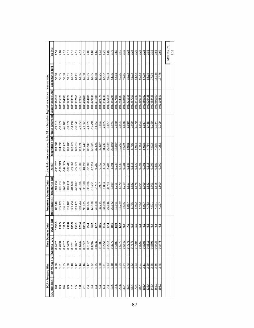
87

* Le

ad

ind

uct

ance

ass

um

ed t

o b

e 3

2 n

H b

ased

on

hig

hes

t re

act

ance

mea

sure

men

t.

DC

_Bia

s (m

A)

Po

rt V

olt

age

(V

)G

amm

a (V

/V)

Dyn

_R (

Ω)

Res

ista

nce

(Ω

)R

eact

ance

(Ω

)X

c (Ω

)M

agn

itu

de

(Ω

)P

has

e (

De

gre

es)

Susc

ep

tan

ce (

1/Ω

)C

apac

itan

ce (

pF)

Tau

(n

s)

0.0

0.0

00

.94

07

16

36

.38

5.6

48

-28

9.2

52

-29

1.2

52

30

3.5

84

-73

.61

30

.00

31

60

17

50

.30

1.5

9

0.3

1.0

10

.78

38

41

2.5

13

5.4

29

-17

6.9

19

-17

8.9

19

22

4.3

95

-52

.87

70

.00

35

53

29

56

.55

2.0

7

0.6

1.0

50

.72

37

31

1.9

13

6.9

19

-14

0.3

05

-14

2.3

05

19

7.4

78

-46

.10

50

.00

36

49

08

58

.08

2.1

3

0.9

1.0

80

.64

39

23

0.8

13

1.1

03

-10

5.4

11

-10

7.4

11

16

9.4

85

-39

.32

70

.00

37

39

27

59

.51

2.1

5

1.2

1.1

00

.57

61

18

5.9

12

1.7

52

-81

.66

8-8

3.6

68

14

7.7

29

-34

.49

70

.00

38

33

78

61

.02

2.1

6

1.5

1.1

20

.50

77

15

3.1

11

1.1

73

-63

.07

7-6

5.0

77

12

8.8

19

-30

.34

30

.00

39

21

61

62

.41

2.1

5

1.8

1.1

40

.44

26

12

9.4

10

1.2

62

-49

.70

6-5

1.7

06

11

3.6

99

-27

.05

00

.00

39

99

69

63

.66

2.1

3

2.1

1.1

60

.37

22

10

9.3

90

.87

5-3

8.3

90

-40

.39

09

9.4

47

-23

.96

30

.00

40

84

08

65

.00

2.1

0

2.4

1.1

70

.31

22

95

.48

2.6

84

-30

.78

6-3

2.7

86

88

.94

7-2

1.6

29

0.0

04

14

40

66

5.9

52

.06

3.4

1.2

20

.12

46

64

.26

0.9

88

-15

.25

1-1

7.2

51

63

.38

1-1

5.7

94

0.0

04

29

43

66

8.3

51

.88

4.4

1.2

5-0

.02

32

47

.74

6.6

08

-7.7

87

-9.7

87

47

.62

4-1

1.8

59

0.0

04

31

50

86

8.6

81

.66

5.4

1.2

8-0

.13

00

38

.53

7.2

15

-3.9

57

-5.9

57

37

.68

9-9

.09

40

.00

41

93

76

66

.75

1.4

2

6.4

1.3

1-0

.22

51

31

.63

1.0

08

-1.8

54

-3.8

54

31

.24

7-7

.08

50

.00

39

47

36

62

.82

1.2

0

7.4

1.3

3-0

.29

14

27

.42

7.0

46

-0.7

84

-2.7

84

27

.18

9-5

.87

70

.00

37

66

18

59

.94

1.0

5

10

.51

.40

-0.4

27

22

0.1

20

.02

20

.60

9-1

.39

12

0.0

70

-3.9

74

0.0

03

45

29

55

4.9

60

.79

15

.61

.48

-0.5

40

01

4.9

15

.00

11

.26

1-0

.73

91

5.0

19

-2.8

20

0.0

03

27

60

65

2.1

40

.60

20

.61

.54

-0.6

07

61

2.2

12

.28

91

.57

0-0

.43

01

2.2

97

-2.0

04

0.0

02

84

38

34

5.2

60

.45

30

.41

.64

-0.6

84

79

.49

.53

51

.71

9-0

.28

19

.53

9-1

.68

80

.00

30

88

08

49

.15

0.3

9

40

.41

.73

-0.7

27

17

.98

.03

71

.85

7-0

.14

38

.03

8-1

.01

90

.00

22

13

15

35

.22

0.2

4

55

.41

.82

-0.7

67

16

.66

.76

51

.88

2-0

.11

86

.76

6-0

.99

90

.00

25

77

59

41

.02

0.2

4

70

.41

.93

-0.7

90

45

.95

.97

21

.87

8-0

.12

25

.97

3-1

.17

00

.00

34

19

31

54

.42

0.2

9

85

.42

.01

-0.8

06

95

.35

.48

21

.90

4-0

.09

65

.48

3-1

.00

30

.00

31

93

45

50

.83

0.2

5

10

5.4

2.1

1-0

.82

03

4.9

5.0

27

1.9

09

-0.0

91

5.0

28

-1.0

37

0.0

03

59

98

25

7.2

90

.26

12

5.4

2.2

0-0

.83

11

4.6

4.7

33

1.8

82

-0.1

18

4.7

34

-1.4

28

0.0

05

26

42

88

3.7

80

.36

14

5.4

2.2

8-0

.83

91

4.4

4.5

01

1.9

01

-0.0

99

4.5

02

-1.2

60

0.0

04

88

43

57

7.7

40

.32

16

5.2

2.3

6-0

.84

25

4.3

4.3

71

1.8

18

-0.1

82

4.3

75

-2.3

84

0.0

09

50

95

01

51

.35

0.6

1

19

5.2

2.4

8-0

.84

78

4.1

4.2

27

1.8

00

-0.2

00

4.2

32

-2.7

09

0.0

11

16

84

91

77

.75

0.6

9

Max

Tau

(n

s)

2.1

6

Tim

e D

om

ain

Dat

aSO

A -

Fo

rwar

d B

ias

Fre

qu

en

cy D

om

ain

Dat

a

88

Appendix D: TDR Validation Measurements

BM Section Response Time

DC_Bias (mA) Dyn_R (Ω) Tau (ns)

200.0 6.2 0.300

130.6 7.5 0.30

75.1 9.3 0.25

10.1 22.5 0.50

4.5 32.0 0.70

0.0 1148.0 1.30

89

Appendix E: Tuning Map Matlab Functions

LASERMEASUREMENT()

% LASERMEASUREMENT() function summary: % This function automates the collection of a tunable VT-DBR laser's % wavelength, power, and spectral content as a function of control port % bias current. The sample point resolution is user defined by inputing

the % desired start, stop, and step of the bias current for the front and

back % mirrors. This data can then be used to generate the laser's tuning

map.

function [ ] =

LaserMeasurement(FMstart,FMstop,FMstep,BMstart,BMstop,... BMstep,startsample) % Determine FMspan and BMspan FMspan = FMstop-FMstart; BMspan = BMstop-BMstart; % Condition variables to avoid erronious operation. floor(startsample); % Configure FM and BM current drivers. %Find a GPIB object. BM = instrfind('Type', 'gpib', 'BoardIndex', 32,

'PrimaryAddress',... 2, 'Tag', ''); FM = instrfind('Type', 'gpib', 'BoardIndex', 32,

'PrimaryAddress',... 1, 'Tag', '');

% Create the GPIB object if it does not exist otherwise use the

object % that was found. if isempty(BM) BM = gpib('AGILENT', 32, 2); else fclose(BM); BM = BM(1); end

if isempty(FM) FM = gpib('AGILENT', 32, 1); else fclose(FM); FM = FM(1); end %Connect to the FM and BM instruments. fopen(BM); fopen(FM);

%Communicating with instruments BM and FM current drivers. fprintf(BM, '*RST'); fprintf(BM, 'LAS:RAN 1'); fprintf(BM, 'LAS:LIM:I1 101');

90

fprintf(BM, 'LAS:MOD:ILBW');

fprintf(FM, '*RST'); fprintf(FM, 'LAS:RAN 1'); fprintf(FM, 'LAS:LIM:I1 101'); fprintf(FM, 'LAS:MOD:ILBW');

% Increments along each axis determined by user input current range

and % step. FMnum = floor(FMspan/FMstep); if rem(FMspan,FMstep)>0.3*FMstep FMnum = FMnum+1; end BMnum = floor(BMspan/BMstep); if rem(BMspan,BMstep)>0.3*BMstep BMnum = BMnum+1; end % If startsample < 2, create new excel data-file called

'TuningMap.xlsx' % unless one already exist. Add new sheet to 'TuningMap.xlsx'. warning off; if startsample < 2; % Display number of samples to be taken fprintf([ num2str((FMnum+1)*(BMnum+1)) ' samples will be taken.']); % Create header object. parameters = 'Sample (#)', 'FM current bias (mA)',... 'BM current bias (mA)', 'Wavelength (nm)', 'Amplitude (dBm)'; % Check to see if 'TuningMap.xls' already exists, if not create it.

Add % new sheet to 'TuningMap.xls'. if exist('TuningMap.xls', 'file') == 0 time = fix(clock); sheetname = [num2str(time(2)) '.' num2str(time(3)) '.'... num2str(time(1)) '_@_' num2str(time(4)) '.'

num2str(time(5))... '.' num2str(time(6))]; xlswrite('TuningMap', parameters(1), sheetname, 'a1:a1'); xlswrite('TuningMap', parameters(2), sheetname, 'b1:b1'); xlswrite('TuningMap', parameters(3), sheetname, 'c1:c1'); xlswrite('TuningMap', parameters(4), sheetname, 'd1:d1'); xlswrite('TuningMap', parameters(5), sheetname, 'e1:e1'); %Delete extra blank sheets xls_sheet_delete(); else %Ensure new sheetname is used and old data is not overwritten. time = fix(clock); sheetname = [num2str(time(2)) '.' num2str(time(3)) '.'... num2str(time(1)) '_@_' num2str(time(4)) '.'

num2str(time(5))... '.' num2str(time(6))]; xlswrite('TuningMap', parameters(1), sheetname, 'a1:a1'); xlswrite('TuningMap', parameters(2), sheetname, 'b1:b1'); xlswrite('TuningMap', parameters(3), sheetname, 'c1:c1'); xlswrite('TuningMap', parameters(4), sheetname, 'd1:d1'); xlswrite('TuningMap', parameters(5), sheetname, 'e1:e1');

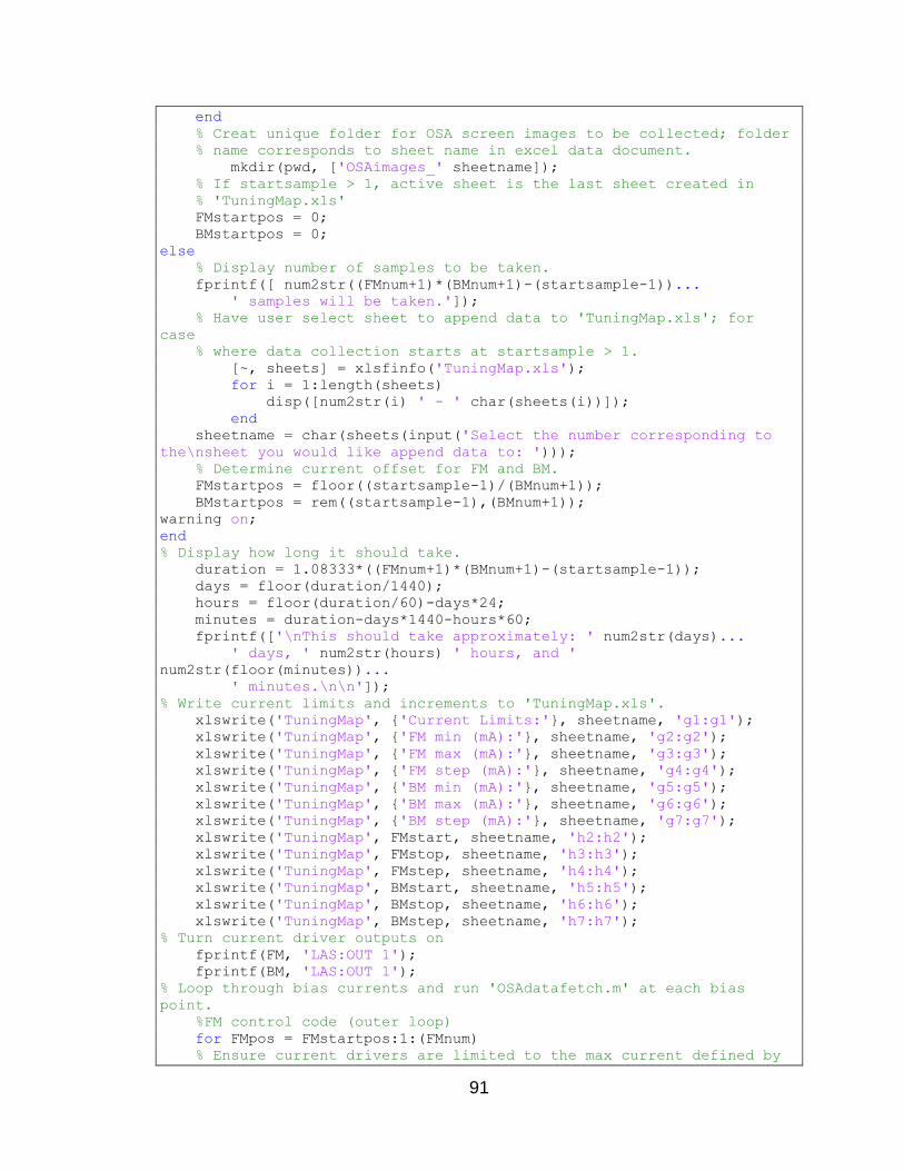
91

end % Creat unique folder for OSA screen images to be collected; folder % name corresponds to sheet name in excel data document. mkdir(pwd, ['OSAimages_' sheetname]); % If startsample > 1, active sheet is the last sheet created in % 'TuningMap.xls' FMstartpos = 0; BMstartpos = 0; else % Display number of samples to be taken. fprintf([ num2str((FMnum+1)*(BMnum+1)-(startsample-1))... ' samples will be taken.']); % Have user select sheet to append data to 'TuningMap.xls'; for

case % where data collection starts at startsample > 1. [~, sheets] = xlsfinfo('TuningMap.xls'); for i = 1:length(sheets) disp([num2str(i) ' - ' char(sheets(i))]); end sheetname = char(sheets(input('Select the number corresponding to

the\nsheet you would like append data to: '))); % Determine current offset for FM and BM. FMstartpos = floor((startsample-1)/(BMnum+1)); BMstartpos = rem((startsample-1),(BMnum+1)); warning on; end % Display how long it should take. duration = 1.08333*((FMnum+1)*(BMnum+1)-(startsample-1)); days = floor(duration/1440); hours = floor(duration/60)-days*24; minutes = duration-days*1440-hours*60; fprintf(['\nThis should take approximately: ' num2str(days)... ' days, ' num2str(hours) ' hours, and '

num2str(floor(minutes))... ' minutes.\n\n']); % Write current limits and increments to 'TuningMap.xls'. xlswrite('TuningMap', 'Current Limits:', sheetname, 'g1:g1'); xlswrite('TuningMap', 'FM min (mA):', sheetname, 'g2:g2'); xlswrite('TuningMap', 'FM max (mA):', sheetname, 'g3:g3'); xlswrite('TuningMap', 'FM step (mA):', sheetname, 'g4:g4'); xlswrite('TuningMap', 'BM min (mA):', sheetname, 'g5:g5'); xlswrite('TuningMap', 'BM max (mA):', sheetname, 'g6:g6'); xlswrite('TuningMap', 'BM step (mA):', sheetname, 'g7:g7'); xlswrite('TuningMap', FMstart, sheetname, 'h2:h2'); xlswrite('TuningMap', FMstop, sheetname, 'h3:h3'); xlswrite('TuningMap', FMstep, sheetname, 'h4:h4'); xlswrite('TuningMap', BMstart, sheetname, 'h5:h5'); xlswrite('TuningMap', BMstop, sheetname, 'h6:h6'); xlswrite('TuningMap', BMstep, sheetname, 'h7:h7'); % Turn current driver outputs on fprintf(FM, 'LAS:OUT 1'); fprintf(BM, 'LAS:OUT 1'); % Loop through bias currents and run 'OSAdatafetch.m' at each bias

point. %FM control code (outer loop) for FMpos = FMstartpos:1:(FMnum) % Ensure current drivers are limited to the max current defined by

92

% user's current settings. if FMpos*FMstep<(FMspan) FMsetpoint = ['LAS:LDI ' num2str(FMpos*FMstep + FMstart)]; fprintf(FM, FMsetpoint); else FMsetpoint = ['LAS:LDI ' num2str(FMspan + FMstart)]; fprintf(FM, FMsetpoint); end %BM control code (inner loop) for BMpos = BMstartpos:1:(BMnum) if BMpos*BMstep<(BMspan) BMsetpoint = ['LAS:LDI ' num2str(BMpos*BMstep +

BMstart)]; fprintf(BM, BMsetpoint); else BMsetpoint = ['LAS:LDI ' num2str(BMspan + BMstart)]; fprintf(BM, BMsetpoint); end

%Determine 'sample_num', call OSAdatafetch and write data %to the 'TuningMap.xls' excel file. pause(1) sample_num = (BMnum+1)*FMpos + (BMpos+1); fprintf(['\nsample# ' num2str(sample_num) '/'... num2str((FMnum+1)*(BMnum+1))]); %Command OSA to find optical signal, take screen-shot, %and return wavelength and amplitude information. [wavelength, amp] = OSAdatafetch(sample_num, sheetname); %Determine bias currents and write to excel file fprintf(FM, 'LAS:LDI?'); FMcurrent = str2double(fscanf(FM)); xlswrite('TuningMap', FMcurrent, sheetname,... ['B' num2str(sample_num+1) ':B'

num2str(sample_num+1)]); fprintf(BM, 'LAS:LDI?'); BMcurrent = str2double(fscanf(BM)); xlswrite('TuningMap', BMcurrent, sheetname,... ['C' num2str(sample_num+1) ':C'

num2str(sample_num+1)]); BMstartpos = 0; % Write sample number, wavelength, and amplitude data % to the 'TuningMap.xls'. xlswrite('TuningMap', sample_num, sheetname,... ['A' num2str(sample_num+1) ':A'

num2str(sample_num+1)]); xlswrite('TuningMap', wavelength, sheetname,... ['D' num2str(sample_num+1) ':D'

num2str(sample_num+1)]); xlswrite('TuningMap', amp, sheetname,... ['E' num2str(sample_num+1) ':E'

num2str(sample_num+1)]); end end % Turn instrument outputs 'off'. fprintf(FM, 'LAS:OUT 0'); fprintf(BM, 'LAS:OUT 0');

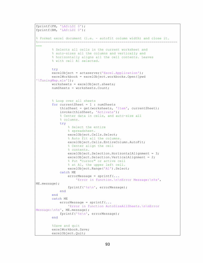
93

fprintf(FM, 'LAS:LDI 0'); fprintf(BM, 'LAS:LDI 0');

% Format excel document (i.e. - autofit column width) and close it. %======================================================================

=== % Selects all cells in the current worksheet and % auto-sizes all the columns and vertically and % horizontally aligns all the cell contents. Leaves % with cell A1 selected.

try excelObject = actxserver('Excel.Application'); excelWorkbook = excelObject.workbooks.Open([pwd

'\TuningMap.xls']); worksheets = excelObject.sheets; numSheets = worksheets.Count;

% Loop over all sheets for currentSheet = 1 : numSheets thisSheet = get(worksheets, 'Item', currentSheet); invoke(thisSheet, 'Activate'); % Center data in cells, and auto-size all % columns. try % Select the entire % spreadsheet. excelObject.Cells.Select; % Auto fit all the columns. excelObject.Cells.EntireColumn.AutoFit; % Center align the cell % contents. excelObject.Selection.HorizontalAlignment = 3; excelObject.Selection.VerticalAlignment = 2; % Put "cursor" or active cell % at A1, the upper left cell. excelObject.Range('A1').Select; catch ME errorMessage = sprintf(... 'Error in function.\n\nError Message:\n%s',

ME.message); fprintf('%s\n', errorMessage); end end catch ME errorMessage = sprintf(... 'Error in function AutoSizeAllSheets.\n\nError

Message:\n%s', ME.message); fprintf('%s\n', errorMessage); end

%Save and quit excelWorkbook.Save; excelObject.Quit;

94

fclose('all');

% Close and clear all objects from memory. close all; clear all; disp('Data collected successfully!')

end

% This function is for communicating with the OSA instrument. Instument

is %directed to acquire the optical signal with the largest power

magnitude; %then the wavelength, power magnitude, and screen capture of the signal

are %returned to the computer. function [wavelength, amp] = OSAdatafetch(sample_num, sheetname)

% Find a GPIB object. OSA = instrfind('Type', 'gpib', 'BoardIndex', 32, 'PrimaryAddress',

4,... 'Tag', '');

% Create the GPIB object if it does not exist otherwise use the object

that % was found. if isempty(OSA) OSA = gpib('AGILENT', 32, 4); else fclose(OSA); OSA = OSA(1); end

% Configure OSA instrument. set(OSA, 'EOIMode', 'on'); set(OSA, 'EOSMode', 'none'); set(OSA, 'InputBufferSize', 500000); set(OSA, 'OutputBufferSize', 500000); set(OSA, 'Timeout', 30.0);

% Connect to OSA instrument. fopen(OSA);

% Initializing OSA instrument: remove write warnings, reset, adjust the % verticle scale to 6.4 dB/div, and perform auto-measure. warning('off','instrument:fread:unsuccessfulRead') fprintf(OSA, '*rst'); fprintf(OSA, 'disp:trac:Y:scal:auto:pdiv 6.4 dB'); fprintf(OSA, 'disp:wind:trac:all:scal:auto; *wai');

% Continually sweep, set span to 2 nm, and set averaging to 20 sweeps.

95

fprintf(OSA, 'init:cont on'); fprintf(OSA, 'sens:wav:span 2 nm'); fprintf(OSA, 'calc1:aver:coun 20'); fprintf(OSA, 'calc1:aver:stat on'); pause(2)

% Move marker to peak, center trace data, adjust reference level to

peak. fprintf(OSA, 'calc:mark1:max'); fprintf(OSA, 'calc:mark1:scen'); fprintf(OSA, 'calc:mark1:srl'); pause(6)

% Query wavelength (nm), query power level (dBm), record to excel file. fprintf(OSA, 'calc:mark1:x?'); wavelength = str2double(fscanf(OSA))*10^9; fprintf(['\nWavelength: ' num2str(wavelength,8) '(nm)']); fprintf(OSA, 'calc:mark1:y?'); amp = str2double(fscanf(OSA)); fprintf(['\nPower: ' num2str(amp,6) '(dBm)\n']);

% Set OSA image data language to 'gif' format, ask for image data, and % suppress data transfer warnings while reading data from OSA. fprintf(OSA, 'HCOP:DEV:LANG ''GIF'''); fprintf(OSA, 'HCOP:DATA?'); raw = fread(OSA);

% Remove initial '#0' characters and EOI character from image data. gooddata = raw(3:(length(raw)-1));

% Creating 'gif' image file containing screen capture sample_num = num2str(sample_num); filename = [ pwd '\OSAimages_' sheetname '\Num' sample_num

'_OSAcap.gif']; fid = fopen(filename, 'w'); fwrite(fid, gooddata); % disp([num2str(length(raw)) ' bytes of image-data transferred to ' % filename]);

% Disconnect all objects. fclose(fid); fclose(OSA);

% Clean up all objects. delete(OSA); clear OSA;

end

% This function deletes the first three excel sheets from a newly

created % 'TuningMap.xls' file.

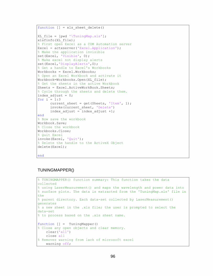
96

function [] = xls_sheet_delete()

XL_file = [pwd '\TuningMap.xls']; xlsfinfo(XL_file); % First open Excel as a COM Automation server Excel = actxserver('Excel.Application'); % Make the application invisible set(Excel, 'Visible', 0); % Make excel not display alerts set(Excel,'DisplayAlerts',0); % Get a handle to Excel's Workbooks Workbooks = Excel.Workbooks; % Open an Excel Workbook and activate it Workbook=Workbooks.Open(XL_file); % Get the sheets in the active Workbook Sheets = Excel.ActiveWorkBook.Sheets; % Cycle through the sheets and delete them. index_adjust = 0; for i = 1:3 current_sheet = get(Sheets, 'Item', 1); invoke(current_sheet, 'Delete') index_adjust = index_adjust +1; end % Now save the workbook Workbook.Save; % Close the workbook Workbooks.Close; % Quit Excel invoke(Excel, 'Quit'); % Delete the handle to the ActiveX Object delete(Excel);

end

TUNINGMAPPER()

% TUNINGMAPPER() function summary: This function takes the data

collected % using LaserMeasurement() and maps the wavelength and power data into % surface plots. The data is extracted from the 'TuningMap.xls' file in

the % parent directory. Each data-set collected by LaserMeasurement()

generates % a new sheet in the .xls file; the user is prompted to select the

data-set % to process based on the .xls sheet name.

function [] = TuningMapper() % Close any open objects and clear memory. clear('all') close all % Removes warning from lack of microsoft excel warning off;

97

% Find available sheets in 'TuningMap.xls' and prompt user to select

one. [~, sheets] = xlsfinfo('TuningMap.xls'); for i = 1:length(sheets) disp([num2str(i) ' - ' char(sheets(i))]); end sheetname = char(sheets(input('Select the number corresponding

to\nthe sheet you would like to process: '))); map = str2double(input('\n1 - Wavelength tuning-map.\n2 - Power

tuning-map.\n3 - Wave & Pwr tuning-map.\nInput number corresponding

to\ndesired tuning-map generation: ', 's')); % Read in current bias and wavelength data from 'TuningMap.xls' excel

file. [wavedata, ~ ]=xlsread('TuningMap.xls',sheetname); FMcurrent = wavedata(2:end,2); BMcurrent = wavedata(2:end,3); wavelength = wavedata(2:end,4); pwr = wavedata(2:end,5); % Give user option to import color-map range from another % tuning-map sheet. a = input('\nWould you like to import the colormap\nscale

from another sheet? (y/n) : ', 's'); switch a case 'y' fprintf('\n') [~, sheets] = xlsfinfo('TuningMap.xls'); for i = 1:length(sheets) disp([num2str(i) ' - ' char(sheets(i))]); end % Have user select sheet crange_sheet = char(sheets(input('Select the sheet

containing the colormap\nscale you''d like to import: '))); % Import colormap range from selected sheet [wavedata, ~

]=xlsread('TuningMap.xls',crange_sheet); cwavelength = wavedata(2:end,4); cpwr = wavedata(2:end,5); % Filter caxis_pwr to remove outliers. cpwrave = sum(cpwr)/length(cpwr); for i = 1:length(cpwr) if cpwr(i)<(cpwrave-5) cpwr(i) = cpwrave-5; end end caxis_wave = [min(cwavelength) max(cwavelength)]; caxis_pwr = [min(cpwr) max(cpwr)]; fprintf('Colormap imported. Generating

figure(s).\n\n') case 'n' fprintf('Default colormap range will be used.\n\n') end warning on; % Determine wavelength and power ranges. % global deltawave global deltapwr deltawave = (max(wavelength)-min(wavelength)); deltapwr = (max(pwr)-min(pwr));

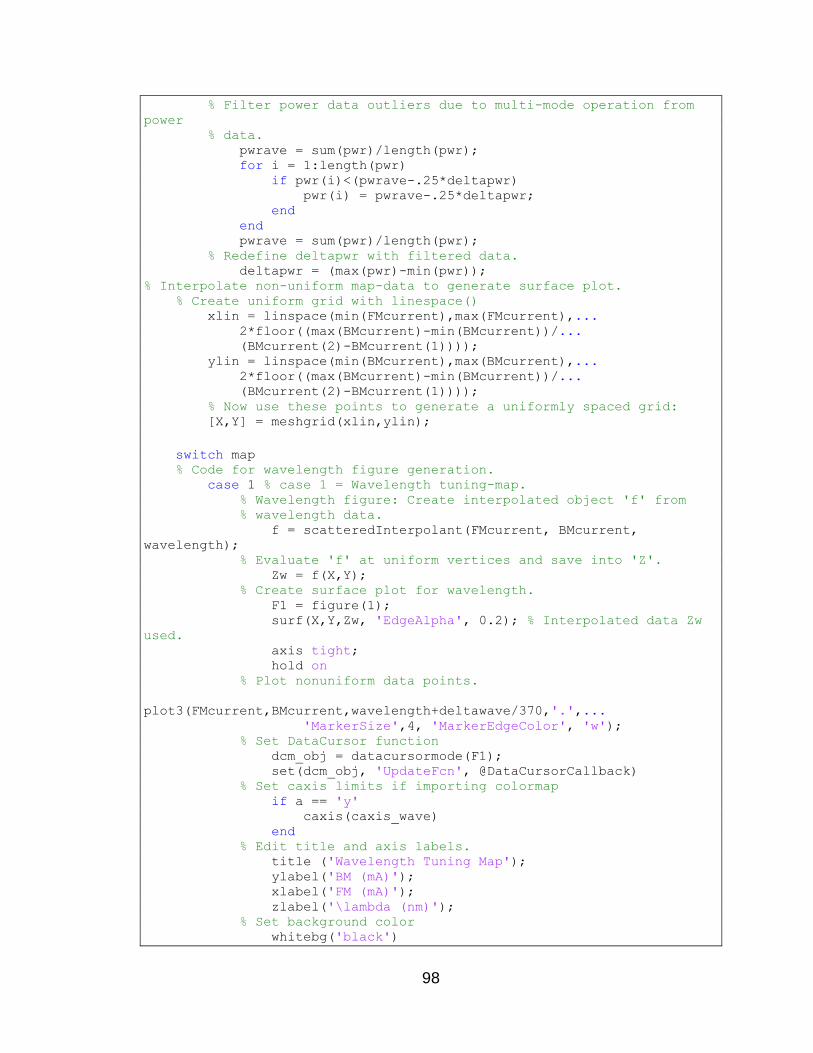
98

% Filter power data outliers due to multi-mode operation from

power % data. pwrave = sum(pwr)/length(pwr); for i = 1:length(pwr) if pwr(i)<(pwrave-.25*deltapwr) pwr(i) = pwrave-.25*deltapwr; end end pwrave = sum(pwr)/length(pwr); % Redefine deltapwr with filtered data. deltapwr = (max(pwr)-min(pwr)); % Interpolate non-uniform map-data to generate surface plot. % Create uniform grid with linespace() xlin = linspace(min(FMcurrent),max(FMcurrent),... 2*floor((max(BMcurrent)-min(BMcurrent))/... (BMcurrent(2)-BMcurrent(1)))); ylin = linspace(min(BMcurrent),max(BMcurrent),... 2*floor((max(BMcurrent)-min(BMcurrent))/... (BMcurrent(2)-BMcurrent(1)))); % Now use these points to generate a uniformly spaced grid: [X,Y] = meshgrid(xlin,ylin);

switch map % Code for wavelength figure generation. case 1 % case 1 = Wavelength tuning-map. % Wavelength figure: Create interpolated object 'f' from % wavelength data. f = scatteredInterpolant(FMcurrent, BMcurrent,

wavelength); % Evaluate 'f' at uniform vertices and save into 'Z'. Zw = f(X,Y); % Create surface plot for wavelength. F1 = figure(1); surf(X,Y,Zw, 'EdgeAlpha', 0.2); % Interpolated data Zw

used. axis tight; hold on % Plot nonuniform data points.

plot3(FMcurrent,BMcurrent,wavelength+deltawave/370,'.',... 'MarkerSize',4, 'MarkerEdgeColor', 'w'); % Set DataCursor function dcm_obj = datacursormode(F1); set(dcm_obj, 'UpdateFcn', @DataCursorCallback) % Set caxis limits if importing colormap if a == 'y' caxis(caxis_wave) end % Edit title and axis labels. title ('Wavelength Tuning Map'); ylabel('BM (mA)'); xlabel('FM (mA)'); zlabel('\lambda (nm)'); % Set background color whitebg('black')

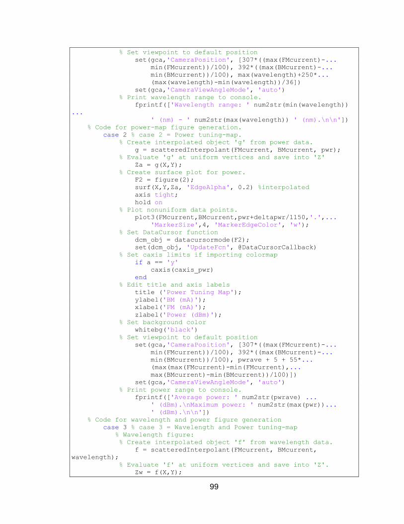
99

% Set viewpoint to default position set(gca,'CameraPosition', [307*((max(FMcurrent)-... min(FMcurrent))/100), 392*((max(BMcurrent)-... min(BMcurrent))/100), max(wavelength)+250*... (max(wavelength)-min(wavelength))/36]) set(gca,'CameraViewAngleMode', 'auto') % Print wavelength range to console. fprintf(['Wavelength range: ' num2str(min(wavelength))

... ' (nm) - ' num2str(max(wavelength)) ' (nm).\n\n']) % Code for power-map figure generation. case 2 % case 2 = Power tuning-map. % Create interpolated object 'g' from power data. g = scatteredInterpolant(FMcurrent, BMcurrent, pwr); % Evaluate 'g' at uniform vertices and save into 'Z' Za = g(X,Y); % Create surface plot for power. F2 = figure(2); surf(X,Y,Za, 'EdgeAlpha', 0.2) %interpolated axis tight; hold on % Plot nonuniform data points. plot3(FMcurrent,BMcurrent,pwr+deltapwr/1150,'.',... 'MarkerSize',4, 'MarkerEdgeColor', 'w'); % Set DataCursor function dcm_obj = datacursormode(F2); set(dcm_obj, 'UpdateFcn', @DataCursorCallback) % Set caxis limits if importing colormap if a == 'y' caxis(caxis_pwr) end % Edit title and axis labels title ('Power Tuning Map'); ylabel('BM (mA)'); xlabel('FM (mA)'); zlabel('Power (dBm)'); % Set background color whitebg('black') % Set viewpoint to default position set(gca,'CameraPosition', [307*((max(FMcurrent)-... min(FMcurrent))/100), 392*((max(BMcurrent)-... min(BMcurrent))/100), pwrave + 5 + 55*... (max(max(FMcurrent)-min(FMcurrent),... max(BMcurrent)-min(BMcurrent))/100)]) set(gca,'CameraViewAngleMode', 'auto') % Print power range to console. fprintf(['Average power: ' num2str(pwrave) ... ' (dBm).\nMaximum power: ' num2str(max(pwr))... ' (dBm).\n\n']) % Code for wavelength and power figure generation case 3 % case 3 = Wavelength and Power tuning-map % Wavelength figure: % Create interpolated object 'f' from wavelength data. f = scatteredInterpolant(FMcurrent, BMcurrent,

wavelength); % Evaluate 'f' at uniform vertices and save into 'Z'. Zw = f(X,Y);

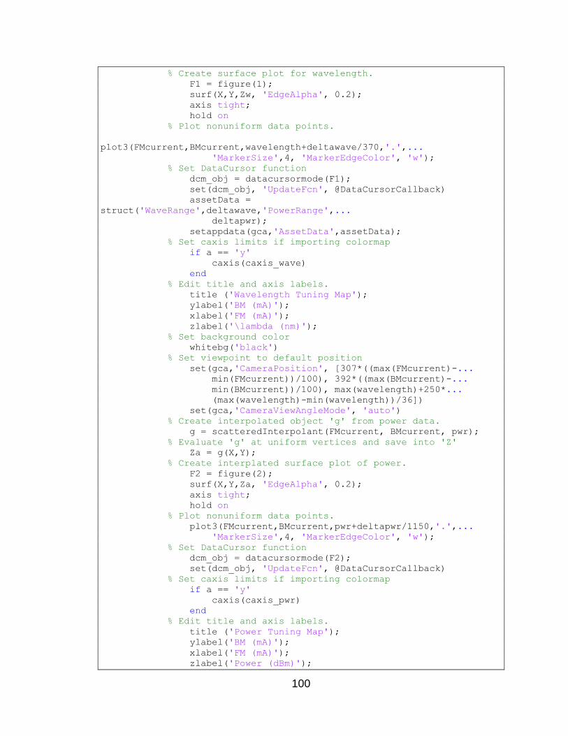
100

% Create surface plot for wavelength. F1 = figure(1); surf(X,Y,Zw, 'EdgeAlpha', 0.2); axis tight; hold on % Plot nonuniform data points.

plot3(FMcurrent,BMcurrent,wavelength+deltawave/370,'.',... 'MarkerSize',4, 'MarkerEdgeColor', 'w'); % Set DataCursor function dcm_obj = datacursormode(F1); set(dcm_obj, 'UpdateFcn', @DataCursorCallback) assetData =

struct('WaveRange',deltawave,'PowerRange',... deltapwr); setappdata(gca,'AssetData',assetData); % Set caxis limits if importing colormap if a == 'y' caxis(caxis_wave) end % Edit title and axis labels. title ('Wavelength Tuning Map'); ylabel('BM (mA)'); xlabel('FM (mA)'); zlabel('\lambda (nm)'); % Set background color whitebg('black') % Set viewpoint to default position set(gca,'CameraPosition', [307*((max(FMcurrent)-... min(FMcurrent))/100), 392*((max(BMcurrent)-... min(BMcurrent))/100), max(wavelength)+250*... (max(wavelength)-min(wavelength))/36]) set(gca,'CameraViewAngleMode', 'auto') % Create interpolated object 'g' from power data. g = scatteredInterpolant(FMcurrent, BMcurrent, pwr); % Evaluate 'g' at uniform vertices and save into 'Z' Za = g(X,Y); % Create interplated surface plot of power. F2 = figure(2); surf(X,Y,Za, 'EdgeAlpha', 0.2); axis tight; hold on % Plot nonuniform data points. plot3(FMcurrent,BMcurrent,pwr+deltapwr/1150,'.',... 'MarkerSize',4, 'MarkerEdgeColor', 'w'); % Set DataCursor function dcm_obj = datacursormode(F2); set(dcm_obj, 'UpdateFcn', @DataCursorCallback) % Set caxis limits if importing colormap if a == 'y' caxis(caxis_pwr) end % Edit title and axis labels. title ('Power Tuning Map'); ylabel('BM (mA)'); xlabel('FM (mA)'); zlabel('Power (dBm)');

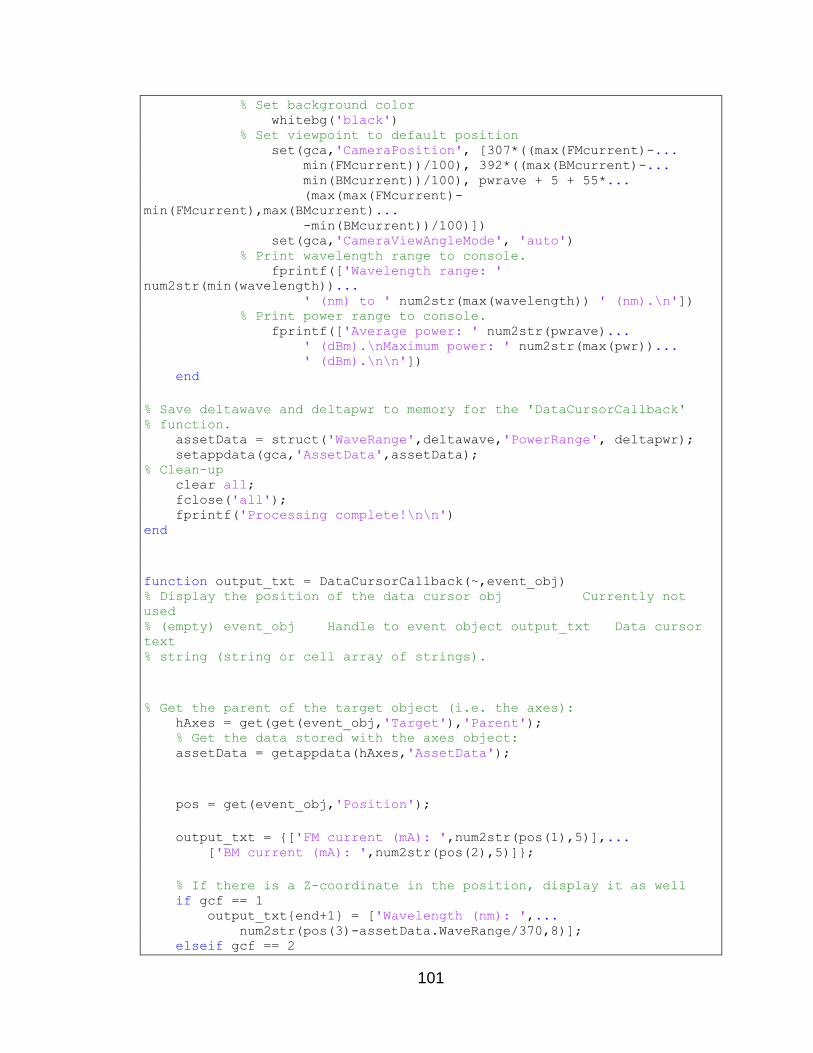
101

% Set background color whitebg('black') % Set viewpoint to default position set(gca,'CameraPosition', [307*((max(FMcurrent)-... min(FMcurrent))/100), 392*((max(BMcurrent)-... min(BMcurrent))/100), pwrave + 5 + 55*... (max(max(FMcurrent)-

min(FMcurrent),max(BMcurrent)... -min(BMcurrent))/100)]) set(gca,'CameraViewAngleMode', 'auto') % Print wavelength range to console. fprintf(['Wavelength range: '

num2str(min(wavelength))... ' (nm) to ' num2str(max(wavelength)) ' (nm).\n']) % Print power range to console. fprintf(['Average power: ' num2str(pwrave)... ' (dBm).\nMaximum power: ' num2str(max(pwr))... ' (dBm).\n\n']) end

% Save deltawave and deltapwr to memory for the 'DataCursorCallback' % function. assetData = struct('WaveRange',deltawave,'PowerRange', deltapwr); setappdata(gca,'AssetData',assetData); % Clean-up clear all; fclose('all'); fprintf('Processing complete!\n\n') end

function output_txt = DataCursorCallback(~,event_obj) % Display the position of the data cursor obj Currently not

used % (empty) event_obj Handle to event object output_txt Data cursor

text % string (string or cell array of strings).

% Get the parent of the target object (i.e. the axes): hAxes = get(get(event_obj,'Target'),'Parent'); % Get the data stored with the axes object: assetData = getappdata(hAxes,'AssetData');

pos = get(event_obj,'Position');

output_txt = ['FM current (mA): ',num2str(pos(1),5)],... ['BM current (mA): ',num2str(pos(2),5)];

% If there is a Z-coordinate in the position, display it as well if gcf == 1 output_txtend+1 = ['Wavelength (nm): ',... num2str(pos(3)-assetData.WaveRange/370,8)]; elseif gcf == 2

102

output_txtend+1 = ['Power (dBm): ',... num2str(pos(3)-assetData.PowerRange/1150,8)]; end

end

TUNINGMAPVID()

% TUNINGMAPVID() function summary: This function creates a video using

a surface % plot of the laser's tuning-map by rotating the the selected figure's

viewpoint % and appending the resulting frame sequence to a video object which is % then saved to the parent directory with the corresponding sheet name % included in the file name.

function [] = TuningMapVid()

% Close any open objects and clear memory. clear('all') close all % Set video format and file destination-path. Format options include: % 'Motion JPEG AVI', 'Motion JPEG 2000','Uncompressed AVI',

and'Archival'. format = 'Uncompressed AVI'; path = 'C:\Users\Greg\Desktop\'; % Determine sheet-names available in the 'TuningMap.xls' file. Prompt

user % to select sheet and ask which map-videos to generate. warning off; % Removes warning from lack of microsoft excel. [~, sheets] = xlsfinfo('TuningMap.xls'); for i = 1:length(sheets) disp([num2str(i) ' - ' char(sheets(i))]); end sheetname = char(sheets(input('Select the number corresponding

to\nthe sheet you would like to process: '))); map = str2double(input('\n1 - Wavelength tuning-map video.\n2 -

Power tuning-map video.\n3 - Wave & Pwr tuning-map videos.\nInput

number corresponding to\ndesired tuning map generation: ', 's')); precision = input('\nWhat is the desired number of\nviewpoint

incriments? (i.e. - any number > 0): '); % Adjust framerate based on user input precision. if precision<=300 framerate = floor(precision/25)+1; elseif precision>300 framerate = 26; end % Read in current bias and wavelength data from 'TuningMap.xls' excel

file. [wavedata,~] = xlsread('TuningMap.xls',sheetname); FMcurrent = wavedata(2:end,2); BMcurrent = wavedata(2:end,3); wavelength = wavedata(2:end,4); pwr = wavedata(2:end,5);

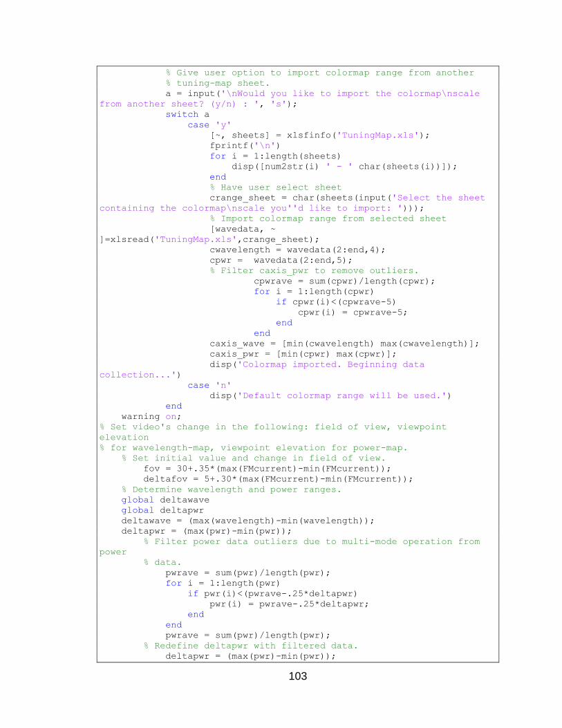
103

% Give user option to import colormap range from another % tuning-map sheet. a = input('\nWould you like to import the colormap\nscale

from another sheet? (y/n) : ', 's'); switch a case 'y' [~, sheets] = xlsfinfo('TuningMap.xls'); fprintf('\n') for i = 1:length(sheets) disp([num2str(i) ' - ' char(sheets(i))]); end % Have user select sheet crange_sheet = char(sheets(input('Select the sheet

containing the colormap\nscale you''d like to import: '))); % Import colormap range from selected sheet [wavedata, ~

]=xlsread('TuningMap.xls',crange_sheet); cwavelength = wavedata(2:end,4); cpwr = wavedata(2:end,5); % Filter caxis_pwr to remove outliers. cpwrave = sum(cpwr)/length(cpwr); for i = 1:length(cpwr) if cpwr(i)<(cpwrave-5) cpwr(i) = cpwrave-5; end end caxis_wave = [min(cwavelength) max(cwavelength)]; caxis_pwr = [min(cpwr) max(cpwr)]; disp('Colormap imported. Beginning data

collection...') case 'n' disp('Default colormap range will be used.') end warning on; % Set video's change in the following: field of view, viewpoint

elevation % for wavelength-map, viewpoint elevation for power-map. % Set initial value and change in field of view. fov = 30+.35*(max(FMcurrent)-min(FMcurrent)); deltafov = 5+.30*(max(FMcurrent)-min(FMcurrent)); % Determine wavelength and power ranges. global deltawave global deltapwr deltawave = (max(wavelength)-min(wavelength)); deltapwr = (max(pwr)-min(pwr)); % Filter power data outliers due to multi-mode operation from

power % data. pwrave = sum(pwr)/length(pwr); for i = 1:length(pwr) if pwr(i)<(pwrave-.25*deltapwr) pwr(i) = pwrave-.25*deltapwr; end end pwrave = sum(pwr)/length(pwr); % Redefine deltapwr with filtered data. deltapwr = (max(pwr)-min(pwr));

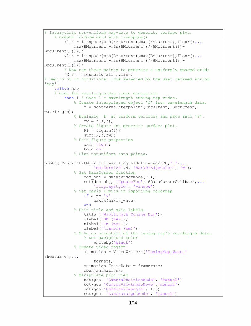
104

% Interpolate non-uniform map-data to generate surface plot. % Create uniform grid with linespace() xlin = linspace(min(FMcurrent),max(FMcurrent),floor((... max(BMcurrent)-min(BMcurrent))/(BMcurrent(2)-

BMcurrent(1)))); ylin = linspace(min(BMcurrent),max(BMcurrent),floor((... max(BMcurrent)-min(BMcurrent))/(BMcurrent(2)-

BMcurrent(1)))); % Now use these points to generate a uniformly spaced grid: [X,Y] = meshgrid(xlin,ylin); % Beginning of conditional code selected by the user defined string

'map'. switch map % Code for wavelength-map video generation case 1 % Case 1 = Wavelength tuning-map video. % Create interpolated object 'f' from wavelength data. f = scatteredInterpolant(FMcurrent, BMcurrent,

wavelength); % Evaluate 'f' at uniform vertices and save into 'Z'. Zw = f(X,Y); % Create figure and generate surface plot. F1 = figure(1); surf(X,Y,Zw); % Edit figure properties axis tight; hold on % Plot nonuniform data points.

plot3(FMcurrent,BMcurrent,wavelength+deltawave/370,'.',... 'MarkerSize',4, 'MarkerEdgeColor', 'w'); % Set DataCursor function dcm_obj = datacursormode(F1); set(dcm_obj, 'UpdateFcn', @DataCursorCallback,... 'DisplayStyle', 'window') % Set caxis limits if importing colormap if a == 'y' caxis(caxis_wave) end % Edit title and axis labels. title ('Wavelength Tuning Map'); ylabel('BM (mA)'); xlabel('FM (mA)'); zlabel('\lambda (nm)'); % Make an animation of the tuning-map's wavelength data. % Set background color whitebg('black') % Create video object animation = VideoWriter(['TuningMap_Wave_'

sheetname],... format); animation.FrameRate = framerate; open(animation); % Manipulate plot view set(gca, 'CameraPositionMode', 'manual') set(gca,'CameraViewAngleMode','manual') set(gca,'CameraViewAngle', fov) set(gca, 'CameraTargetMode', 'manual')

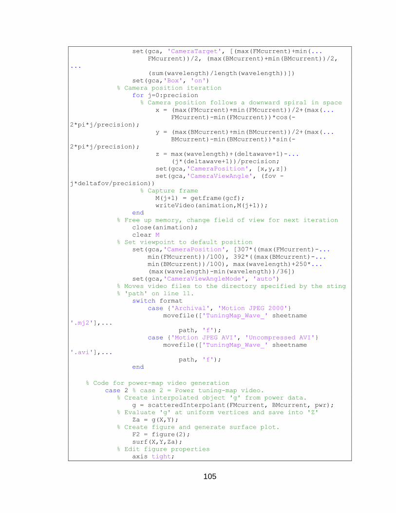
105

set(gca, 'CameraTarget', [(max(FMcurrent)+min(... FMcurrent))/2, (max(BMcurrent)+min(BMcurrent))/2,

... (sum(wavelength)/length(wavelength))]) set(gca,'Box', 'on') % Camera position iteration for j=0:precision % Camera position follows a downward spiral in space x = (max(FMcurrent)+min(FMcurrent))/2+(max(... FMcurrent)-min(FMcurrent))*cos(-

2*pi*j/precision); y = (max(BMcurrent)+min(BMcurrent))/2+(max(... BMcurrent)-min(BMcurrent))*sin(-

2*pi*j/precision); z = max(wavelength)+(deltawave+1)-... (j*(deltawave+1))/precision; set(gca,'CameraPosition', [x,y,z]) set(gca,'CameraViewAngle', (fov -

j*deltafov/precision)) % Capture frame M(j+1) = getframe(gcf); writeVideo(animation,M(j+1)); end % Free up memory, change field of view for next iteration close(animation); clear M % Set viewpoint to default position set(gca,'CameraPosition', [307*((max(FMcurrent)-... min(FMcurrent))/100), 392*((max(BMcurrent)-... min(BMcurrent))/100), max(wavelength)+250*... (max(wavelength)-min(wavelength))/36]) set(gca,'CameraViewAngleMode', 'auto') % Moves video files to the directory specified by the sting % 'path' on line 11. switch format case 'Archival', 'Motion JPEG 2000' movefile(['TuningMap_Wave_' sheetname

'.mj2'],... path, 'f'); case 'Motion JPEG AVI', 'Uncompressed AVI' movefile(['TuningMap_Wave_' sheetname

'.avi'],... path, 'f'); end

% Code for power-map video generation case 2 % case 2 = Power tuning-map video. % Create interpolated object 'g' from power data. g = scatteredInterpolant(FMcurrent, BMcurrent, pwr); % Evaluate 'g' at uniform vertices and save into 'Z' Za = g(X,Y); % Create figure and generate surface plot. F2 = figure(2); surf(X,Y,Za); % Edit figure properties axis tight;

106

hold on % Plot nonuniform data points. plot3(FMcurrent,BMcurrent,pwr+deltapwr/1150,'.',... 'MarkerSize',4, 'MarkerEdgeColor', 'w'); % Set DataCursor function dcm_obj = datacursormode(F2); set(dcm_obj, 'UpdateFcn', @DataCursorCallback,... 'DisplayStyle', 'window') % Set caxis limits if importing colormap if a == 'y' caxis(caxis_pwr) end % Edit title and axis labels. title ('Power Tuning Map'); ylabel('BM (mA)'); xlabel('FM (mA)'); zlabel('Power (dBm)'); % Make an animation of the tuning-map's power power data. % Set background color whitebg('black') % Create video object animation = VideoWriter(['TuningMap_Pwr_'

sheetname],... format); animation.FrameRate = framerate; open(animation); % Manipulate plot view set(gca, 'CameraPositionMode', 'manual') set(gca,'CameraViewAngleMode','manual') set(gca,'CameraViewAngle', fov) set(gca, 'CameraTargetMode', 'manual') set(gca, 'CameraTarget', [(max(FMcurrent)+min(... FMcurrent))/2,

(max(BMcurrent)+min(BMcurrent))/2,... (sum(pwr)/length(pwr))]) set(gca,'Box', 'on') % Camera position iteration for j=0:precision % Camera position follows a downward spiral in space x = (max(FMcurrent)+min(FMcurrent))/2+(max(... FMcurrent)-min(FMcurrent))*cos(-

2*pi*j/precision); y = (max(BMcurrent)+min(BMcurrent))/2+(max(... BMcurrent)-min(BMcurrent))*sin(-

2*pi*j/precision); z = max(pwr)+deltapwr-(j*deltapwr)/precision; set(gca,'CameraPosition', [x,y,z]) set(gca,'CameraViewAngle',... (fov - j*deltafov/precision)) % Capture frame M(j+1) = getframe(gcf); writeVideo(animation,M(j+1)); end % Free up memory, change field of view for next iteration close(animation); clear M % Set viewpoint to default position

107

set(gca,'CameraPosition', [307*((max(FMcurrent)-... min(FMcurrent))/100), 392*((max(BMcurrent)-... min(BMcurrent))/100), pwrave + 5 + 55*(max(max(... FMcurrent)-min(FMcurrent),max(BMcurrent)-... min(BMcurrent))/100)]) set(gca,'CameraViewAngleMode', 'auto') % Moves video files to the directory specified by the sting % 'path' on line 11. switch format case 'Archival', 'Motion JPEG 2000' movefile(['TuningMap_Pwr_' sheetname

'.mj2'],... path, 'f', 'f'); case 'Motion JPEG AVI', 'Uncompressed AVI' movefile(['TuningMap_Pwr_' sheetname

'.avi'],... path, 'f'); end

% Code for wavelength and power tuning-map video generation. case 3 % case 3 = Wave and Pwr tuning-map videos are

generated. % Code for wavelength-map video generation Create

interpolated % object 'f' from wavelength data. f = scatteredInterpolant(FMcurrent, BMcurrent,

wavelength); % Evaluate 'f' at uniform vertices and save into 'Z'. Zw = f(X,Y); % Create figure, generate surface plot, and edit figure

properties. F1 = figure(1); surf(X,Y,Zw); axis tight; hold on % Plot nonuniform data points.

plot3(FMcurrent,BMcurrent,wavelength+deltawave/370,'.',... 'MarkerSize',4, 'MarkerEdgeColor', 'w'); % Set DataCursor function dcm_obj = datacursormode(F1); set(dcm_obj, 'UpdateFcn', @DataCursorCallback,... 'DisplayStyle', 'window') % Set caxis limits if importing colormap if a == 'y' caxis(caxis_wave) end % Edit title and axis labels. title ('Wavelength Tuning Map'); ylabel('BM (mA)'); xlabel('FM (mA)'); zlabel('\lambda (nm)'); % Make an animation of the tuning-map's wavelength data. % Set background color whitebg('black') % Create video object

108

animation = VideoWriter(['TuningMap_Wave_'

sheetname],... format); animation.FrameRate = framerate; open(animation); % Manipulate plot view set(gca, 'CameraPositionMode', 'manual') set(gca,'CameraViewAngleMode','manual') set(gca,'CameraViewAngle', fov) set(gca, 'CameraTargetMode', 'manual') set(gca, 'CameraTarget', [(max(FMcurrent)+min(... FMcurrent))/2, (max(BMcurrent)+min(BMcurrent))/2,

... (sum(wavelength)/length(wavelength))]) set(gca,'Box', 'on') % Camera position iteration for j=0:precision % Camera position follows a downward spiral in space x = (max(FMcurrent)+min(FMcurrent))/2+(max(... FMcurrent)-min(FMcurrent))*cos(-

2*pi*j/precision); y = (max(BMcurrent)+min(BMcurrent))/2+(max(... BMcurrent)-min(BMcurrent))*sin(-

2*pi*j/precision); z = max(wavelength)+(deltawave+1)-... (j*(deltawave+1))/precision; set(gca,'CameraPosition', [x,y,z]) set(gca,'CameraViewAngle', (fov -

j*deltafov/precision)) % Capture frame M(j+1) = getframe(gcf); writeVideo(animation,M(j+1)); end % Free up memory, change field of view for next iteration close(animation); clear M % Set viewpoint to default position set(gca,'CameraPosition', [307*((max(FMcurrent)-min(... FMcurrent))/100), 392*((max(BMcurrent)-min(... BMcurrent))/100), max(wavelength)+250*(max(... wavelength)-min(wavelength))/36]) set(gca,'CameraViewAngleMode', 'auto') % Moves video files to the directory specified by the sting % 'path' on line 11. switch format case 'Archival', 'Motion JPEG 2000' movefile( ['TuningMap_Wave_' sheetname

'.mj2'],... path, 'f'); case 'Motion JPEG AVI', 'Uncompressed AVI' movefile( ['TuningMap_Wave_' sheetname

'.avi'],... path, 'f'); end % Create interpolated object 'g' from power data. g = scatteredInterpolant(FMcurrent, BMcurrent, pwr); % Evaluate 'g' at uniform vertices and save into 'Z'

109

Za = g(X,Y); % Create figure, initialize viewpoint, and generate surface % plot. F2 = figure(2); % Generate surface with uniform vertices from interpolated % data. surf(X,Y,Za); % Edit figure properties axis tight; hold on % Plot nonuniform data points. plot3(FMcurrent,BMcurrent,pwr+deltapwr/1150,'.',... 'MarkerSize',4, 'MarkerEdgeColor', 'w'); % Set DataCursor function dcm_obj = datacursormode(F2); set(dcm_obj, 'UpdateFcn', @DataCursorCallback,... 'DisplayStyle', 'window') % Set caxis limits if importing colormap if a == 'y' caxis(caxis_pwr) end % Edit title and axis labels. title ('Power Tuning Map'); ylabel('BM (mA)'); xlabel('FM (mA)'); zlabel('Power (dBm)'); % Make an animation of the tuning-map's power power data. whitebg('black') % Create video object animation = VideoWriter(['TuningMap_Pwr_' sheetname],

format); animation.FrameRate = framerate; open(animation); % Manipulate plot view set(gca, 'CameraPositionMode', 'manual') set(gca,'CameraViewAngleMode','manual') set(gca,'CameraViewAngle', fov) set(gca, 'CameraTargetMode', 'manual') set(gca, 'CameraTarget', [(max(FMcurrent)+min(... FMcurrent))/2,

(max(BMcurrent)+min(BMcurrent))/2,... (sum(pwr)/length(pwr))]) set(gca,'Box', 'on') % Camera position iteration for j=0:precision % Camera position follows a downward spiral in space x = (max(FMcurrent)+min(FMcurrent))/2+(max(... FMcurrent)-min(FMcurrent))*cos(-

2*pi*j/precision); y = (max(BMcurrent)+min(BMcurrent))/2+(max(... BMcurrent)-min(BMcurrent))*sin(-

2*pi*j/precision); z = max(pwr)+deltapwr-(j*deltapwr)/precision; set(gca,'CameraPosition', [x,y,z]) set(gca,'CameraViewAngle',... (fov - j*deltafov/precision)) % Capture frame

110

M(j+1) = getframe(gcf); writeVideo(animation,M(j+1)); end close(animation); clear M % Set viewpoint to default position set(gca,'CameraPosition', [307*((max(FMcurrent)-min(... FMcurrent))/100), 392*((max(BMcurrent)-min(... BMcurrent))/100), pwrave + 5 + 55*(max(max(... FMcurrent)-min(FMcurrent),max(BMcurrent)-min(... BMcurrent))/100)]) set(gca,'CameraViewAngleMode', 'auto') % Moves video files to the directory specified by the sting % 'path' on line 11. switch format case 'Archival', 'Motion JPEG 2000' movefile(['TuningMap_Pwr_' sheetname

'.mj2'],... path, 'f'); case 'Motion JPEG AVI', 'Uncompressed AVI' movefile(['TuningMap_Pwr_' sheetname

'.avi'],... path, 'f'); end end fprintf('\nProcessing complete!\n\n') end

function output_txt = DataCursorCallback(~,event_obj) % This function displays the position of the data cursor object.

global deltawave global deltapwr pos = get(event_obj,'Position');

output_txt = ['FM current (mA): ',num2str(pos(1),5)],... ['BM current (mA): ',num2str(pos(2),5)]; % If there is a Z-coordinate in the position, display it as well if gcf == 1 output_txtend+1 = ['Wavelength (nm): ',... num2str(pos(3)-deltawave/370,8)]; elseif gcf == 2 output_txtend+1 = ['Power (dBm): ',... num2str(pos(3)-deltapwr/1150,8)]; end end

111

Appendix F: Neptune - Tuning Map Collection and Data

The following file icon links to the embedded “TuningMap.xls” file which

contains all the tabulated tuning map data collected from the Neptune laser. To

access the data, ensure excel is installed on your computer and double click the

file below.

TuningMap.xls

To analyze the data, have MatLab installed on your computer and use the

“TuningMapper()” function below. The “TuningMap.xls” file must be copied to the

same directory as the function.

To create a novel video of a tuning map, use the “TuningMapVid()”

MatLab function below. Again, the “TuningMap.xls” file must be in the same

directory as the function.

The MatLab function “LaserMeasurement()” below is a useful tool for

future VT-DBR tuning map collection.

112

Appendix G: Neptune - SMSR Screen Captures

Measurement FM Bias (mA) BM Bias (mA) Wavelength (nm) SMSR (dB)

1 0 0 1302.93 43.1

2 0 41.72 1291.13 42.2

3 38.42 41.72 1300.73 40.6

4 68.71 0 1306.03 38.7

113

Appendix H: Neptune - Additional OSA and Linewidth Measurements

114

115

116

Appendix I: VTL-2 - SMSR Screen Captures

Measurement FM Bias (mA) BM Bias (mA) Wavelength (nm) SMSR (dB)

1 0 0 1302.93 43.1

2 0 41.72 1291.13 42.2

3 38.42 41.72 1300.73 40.6

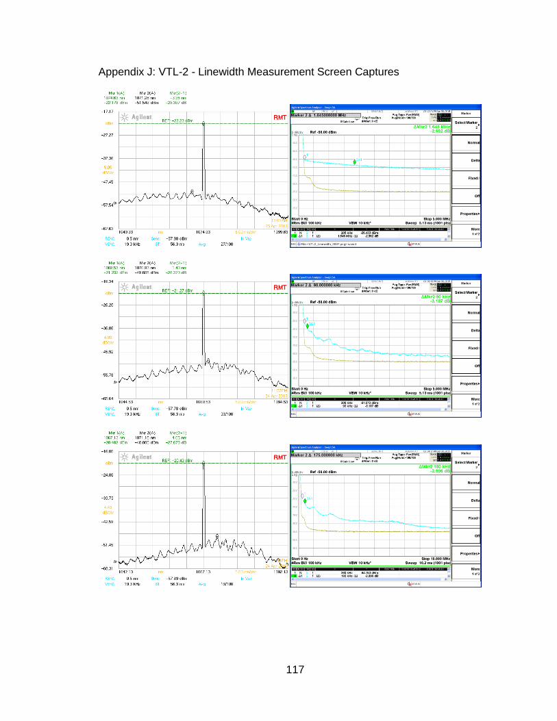
117

Appendix J: VTL-2 - Linewidth Measurement Screen Captures

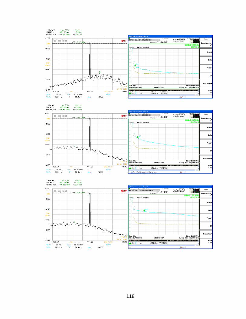
118

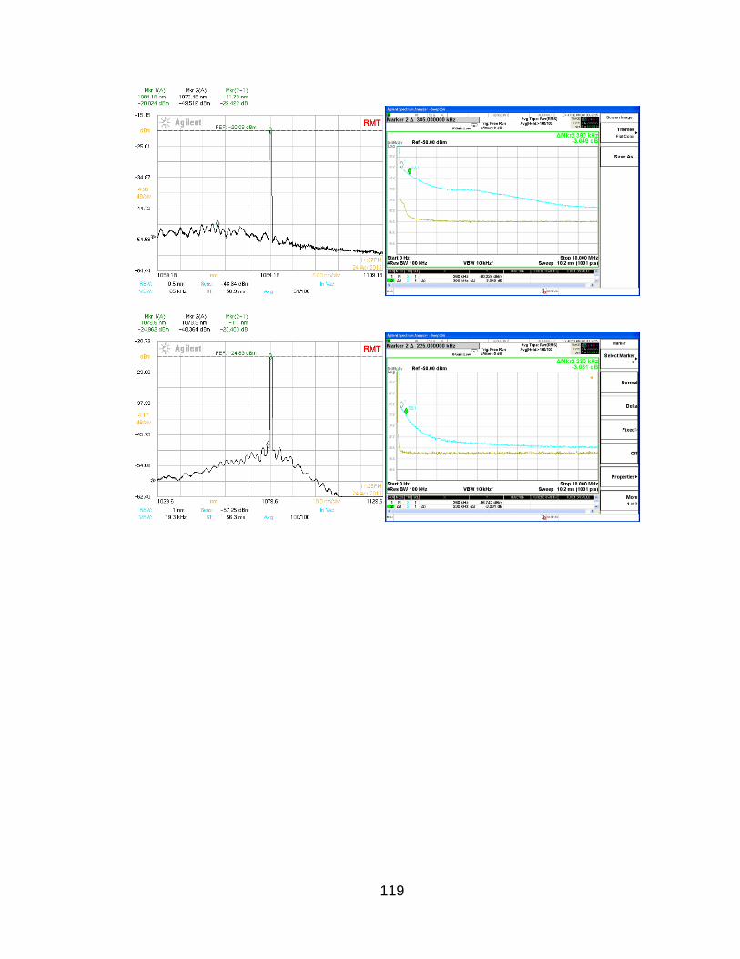
119

120

Appendix K: TDR, FDR, and RLC Data of Neptune Laser

The following icon links to a “.zip” file that contains all the FDR, TDR, and

RLC measurements of the Neptune laser. To open the file, ensure a software

decompression program like WinRar or 7zip is installed on your computer; then,

click the icon below.

Neptune TDR, FDR, and RLC Data.zip

121

Appendix L: TDR, FDR, and RLC Data of VTL-2 Laser

The following icon links to a “.zip” file that contains all the FDR, TDR, and

RLC measurements of the VTL-2 laser. To open the file, ensure a software

decompression program like WinRar or 7zip is installed on your computer; then,

click the icon below.

VTL2 TDR, FDR, and RLC Data.zip

122

Appendix M: Photograph of Automated Tuning Map Collection

123

Appendix N: Photograph of Photonics Lab Workstation