Characterization of the biaxial fatigue behaviour on ...ijame.ump.edu.my/images/Volume 13 Issue 1 June 2016/12_mohamed … · ... Cyclic hardening; maximum shear ... to that associated

International Journal of Automotive and Mechanical Engineering (IJAME)

ISSN: 2229-8649 (Print); ISSN: 2180-1606 (Online);

Volume 13, Issue 1 pp. 3262-3277, June 2016

©Universiti Malaysia Pahang Publishing

DOI: http://dx.doi.org/10.15282/ijame.13.1.2016.12.0272

3262

Characterization of the biaxial fatigue behaviour on medium carbon steel using the

strain-life approach

S.A.N. Mohamed*, S. Abdullah, A. Arifin, A.K. Ariffin, and M.M. Padzi

Faculty of Engineering & Built Environment,

Universiti Kebangsaan Malaysia, 43600 Bangi, Selangor, Malaysia

Email: [email protected]

Phone: +60389118390; Fax: +60389259659

ABSTRACT

This study aims to investigate the fatigue behaviour and determine the fatigue life

prediction under biaxial loading. Fatigue tests were performed according to ASTM

2207-02 and the values of tensile stresses are selected from the ultimate tensile strength

which is 0.5 Su, 0.6 Su, 0.7 Su, 0.8 Su and 0.9 Su, while the torsion angle representing the

shear stresses acting was set at 15 degrees. The biaxial fatigue test was conducted using

a combination of two types of stresses acting on the same frequency, namely 1 Hz, on

smooth specimens made from medium carbon steel. The biaxial fatigue lives of the

specimens are recorded when the specimen has completely fractured. The results

indicate that the observed fatigue lives are in good agreement with the predicted lives by

using the Coffin–Manson, Morrow, and Smith–Watson–Topper strain-based models.

Mohr’s circle approach was used to determine the maximum shear stress and principal

normal stress. The maximum shear stress increased from 457 MPa to 486 MPa with the

increment of principal normal stress from 612 MPa to 767 MPa. The principal stresses,

maximum shear stresses, and energy dissipated were used to explain and describe the

behaviour of biaxial fatigue. Both stresses are inversely proportional to the fatigue life.

Meanwhile, the energy is linearly proportional to the stress applied, where the values

increase in the range 500 kJ/m3 to 605 kJ/m3. Thus, the basic understanding of the

material behaviour may be used in the processes of declaring component service lives

and the fatigue life prediction of a particular automotive component. Therefore, the cost

incurred can be reduced for the development process in material engineering.

Keywords: Cyclic hardening; maximum shear stress; multiaxial fatigue; principal

normal stress; stress–strain hysteresis curve.

INTRODUCTION

Many engineering components and structures, such as axles, crankshafts, turbine discs,

and blades, are exposed to complex and combined service loads that cause local

multiaxial stress states on the critical material element. The accuracy of fatigue life

estimation should be increased to understand the mechanism of damage accumulation

subjected to service multiaxial loading [1]. Under service multiaxial loading,

microscopic cracks can form and grow until macroscopic cracks are formed, thus

causing damage to the component and structure. The behaviour of crack formation and

propagation until the final fracture of materials under multiaxial stress states is different

from that under the uniaxial stress state [2]. Therefore, multiaxial fatigue has become a

popular topic in the past 20 years because of its great importance in mechanical design.

http://dx.doi.org/10.15282/ijame.13.1.2016.12.0272

mailto:sityainy@

Mohamed et al. /International Journal of Automotive and Mechanical Engineering 13(1) 2016 3262-3277

3263

Some multiaxial fatigue models have been proposed for the prediction of multiaxial

fatigue life [3-5]. A multiaxial fatigue model based on stress components was

established by Shang et al. [6] using the linear relationship between the maximum

normal stress and shear amplitude. The critical plane approach in multiaxial fatigue is

based on the physical observation of crack initiation and growth in a particular plane

assisted by the parameters in combinations involving damage to normal and shear stress

on a plane [7, 8].

The automobile industries are always interested in innovations or research and

development on the improvement of engine performance and operational service life to

fulfill market expectations. Engine components are subjected to constant to varying

loads, which also vary in direction and cause component failure. The connecting rod

plays an important role in the operation of the crankshaft in the engine. This component

is connected to the piston in the engine to transmit the thrust of the piston to the

crankshaft, thus converting the reciprocating motion into rotary motion in the operation.

Other parts, such as the pin-end, shank section, crank-end, and bolt, are attached to

provide a good clamp. Therefore, this component is considered to be exposed to

complicated loading and the main failure modes of connecting rods are fatigue fracture,

excessive deformation, and wear [9]. Developing an appropriate design that suits a

series of multiaxial workloads is complicated [10]. Hence, the failure attributed to

broken connecting rods has led researchers to investigate this matter further. A study on

the design of a connecting rod presented a resistant method of failure on connecting rod

design that improved the fatigue life slightly [11]. It was found that the occurrence of

fatigue phenomena is closely related to the appearance of cyclic stresses within the

connecting rod body.

Damage parameters have been proposed to predict multiaxial fatigue failure and

most of them are limited to certain load cases [12]. The multi-axis analysis approach

can be divided into three categories based on the stress, strain and energy [8]. In

considering the strain measurement, it is good to correlate the parameters with the

fatigue life [13]. The strain-based approach can be considered as an approach which

describes the overall behaviour of both the elastic and inelastic region where applicable,

to detect the local plastic strain of stress concentration with the ability to change the

input parameters such as the load history, geometry and attributes to predict the

monotonic and cyclic fatigue life of components [5, 8, 14]. The strain–life approach

considers the nominal elastic stresses and how they are related to the life. The elastic–

plastic load stress and strain represents a more fundamental approach to determine the

number of cycles required to initiate a small engineering crack [15].

Most of the existing multiaxial fatigue analyses were developed by using a stress-

based approach to predict fatigue for high-cycle fatigue (HCF). The disadvantage of the

stress-life analysis method is that more consideration is placed on the nominal elastic

stresses than on the plasticity effect. Hence, the method provides poor accuracy for low-

cycle fatigue (LCF). The strain-based life prediction method provides a detailed analysis

involving plastic deformation at a localized region and can be used proactively for LCF

life prediction in the initial design stage. Therefore, this inspired the authors to move

forward with the present investigation on the biaxial fatigue life assessment of

automotive components by using the strain-based approach. The main purpose of this

study is to determine the fatigue behaviour of steel under biaxial constant amplitude

loading (tension/torsion). An experiment was conducted on a solid mild steel rod to

characterize the biaxial fatigue behaviour in a strain–life curve. The correlation between

fracture was defined. Furthermore, the relationship between principal normal stress and

Characterization of the biaxial fatigue behaviour on medium carbon steel using the strain-life approach

3264

maximum shear stress on the activated plane shows proportional linear increments to

the applied load. The energy dissipated during the failure is illustrated in the stress–

strain hysteresis loop. The area under the loop became larger with increasing applied

loads.

THEORETICAL BACKGROUND

The analysis and design of components by using stress-based fatigue life is a

conservative approach for a situation wherein only elastic stresses and strains are

present. However, most of the components with stress concentration typically result in

local plastic deformation. Under this condition, the strain-based approach is adopted for

an effective prediction of the fatigue life of a component. On the basis of the proposal

by Niesłony and Böhm [16], the relation of the strain amplitude (a ) and fatigue life in

reversals to failure (2Nf) can be expressed mathematically in the following form:

'

'2 2b cfe p

a a a f f fN NE

(1)

Equation (1) is called the strain–life equation, where '

f is the fatigue strength

coefficient, b is the fatigue strength exponent, ε’f is the fatigue ductility coefficient, c is

the fatigue ductility exponent, and E is the modulus of elasticity. This equation is the

foundation for the strain-based approach to fatigue. This equation is also the summation

of two separate curves for the elastic and plastic strain amplitudes. Niesłony and Böhm

[16] proposed another relationship when the mean stress effect is taken into account:

'

'2 2b cf me p

a a a f f fN NE

(2)

when the elastic part of the strain–life curve is modified by the normal mean stress, σm .

[17] proposed the following mean stress correction:

2

' ' '

max 2 2 2b b c

a f f f f fE N E N

(3)

where max is the maximum stress and a is the strain amplitude.

The problem of stress under combined loading can be simplified by first

determining the states of stress caused by the individual loadings. Hence, the axial stress

is calculated as follows:

a

P

A (4)

where P represents the amplitude load and A refers to the original minimum cross-

sectional specimen area. Meanwhile, the shear stress due to torque is calculated as

follows:

max 3

16

original

T

D

(5)

where T represents torque and Doriginal represents the original specimen test diameter.

The most used equivalent stress criteria for ductile steels in the LCF and medium-

cycle fatigue areas are the von Mises (σa EQ vM) and Tresca (σa EQ T) criteria. Von Mises

theory was proposed by Huber in 1904 and was further developed by von Mises in 1913

and Hencky in 1925 [18]. Von Mises theory denotes that failure by yielding occurs


3265

when, at any point in the body, the distortion energy per unit volume in a state of

combined stress becomes equal to that associated with yielding in a simple tension test.

The Tresca criterion was proposed by Tresca (1814–1885) [6]. This criterion predicts

that yielding will start when the maximum shearing stress in the material is equal to the

maximum shear stress at yielding in a simple tension test. For combined tension and

torsion in phase loading, these criteria are described by the following equation:

1

2 2 2

max a am (6)

where σa, τa = normal stress, shear stress loading amplitude; m2 = 3 for the von Mises

criterion and m2 = 4 for the Tresca criterion. The equivalent strain is defined as follows:

12 2

2

3

aaEQ a

(7)

The construction of Mohr’s circle is one of the few graphical techniques still used

in engineering and provides a simple and clear picture of an otherwise complicated

analysis. This circle is usually referred to as Mohr’s circle after the German civil

engineer Otto Mohr (1835–1918). He developed the graphical technique for drawing the

circle in 1882 [9]. Mohr diagrams can conveniently illustrate the relationship between

the plane orientation and the values of normal/shear stress. The horizontal axis contains

the possible values for the normal stresses, whereas the vertical axis contains the values

for the shear stresses. The Mohr circle completely represents the state of stress at a point

in terms of the normal and shear components. By substituting σxx, σyy, and τxy in the

equation, the principal normal and maximum shear stresses can be calculated as

follows:

12 2

2

1,22 2

xx yy xxxy

(8)

1 2 2 3 3 1

max , ,2 2 2

xy

(9)

In constructing Mohr’s circle, the centre and radius of the circle are calculated as

follows:

2

xx yy

ave

(10)

1

2 2

ave xyR (11)

Fatigue life can be characterized by steady-state behaviour. The stress–strain

relationship becomes stable after rapid hardening or softening in the initial cycles

corresponding to the first several percentages of the total fatigue life. The cyclic stable

stress–strain response is the hysteresis loop. The hysteresis loop, defined by the total

strain range (Δε) and the total stress range (Δσ), represents the elastic plus plastic work

on a material undergoing loading and unloading. Masing’s assumption states that the

stress amplitude versus strain amplitude curve can be expressed by the cyclic stress–

strain curve:

1'

'

ne p a a

a a aE K

(12)


3266

where E = elastic modulus, K’ = cyclic strength coefficient, and n’ = cyclic strain

hardening exponent. To determine the change in stress, the following Masing’s model is

used:

1'

2'

n

E K

(13)

MATERIAL AND METHODS

The characterization of the fatigue life was conducted on mild steel. This material is a

common form of steel that provides material properties that are acceptable for many

applications. Solid specimens with 6 mm diameter were designed to follow the

specification in the ASTM E8-01 (Figure 1). The chemical composition results are

shown in Table 1 [19]. Subsequently, the specimens underwent a tensile test according

to the ASTM E466 through the use of a universal testing machine (Figure 2) with a 100

kN load cell capacity. The purpose of the test is to determine the monotonic properties

of the material. Biaxial testing was performed by using the servo-hydraulic biaxial

fatigue test machine with a 25 kN load cell capacity (Figure 3). Testing was conducted

following the requirements in ASTM E2207-02 on estimating the fatigue lives of

materials under combined axial–torsional loading with load-controlled conditions. The

testing was performed by using a sinusoidal waveform at a constant cyclic frequency of

1 Hz [18]. A set of applied stresses for the biaxial cyclic test was chosen in the range of

0.5 Su to 0.9 Su. However, torsion was set at approximately 15° for the twist angle

(clockwise–anticlockwise) for all tension loads.

Table 1. Chemical composition of mild steel.

Composition Value (%)

Carbon, C 0.45

Manganese, Mn 0.4

Sulphur, S 0.015 max

Silicon, Si 0.12

Phosphorus, P 0.015 max

Figure 1. Specimen image after polishing process for both tensile and cyclic testing.

Hexagon grips


3267

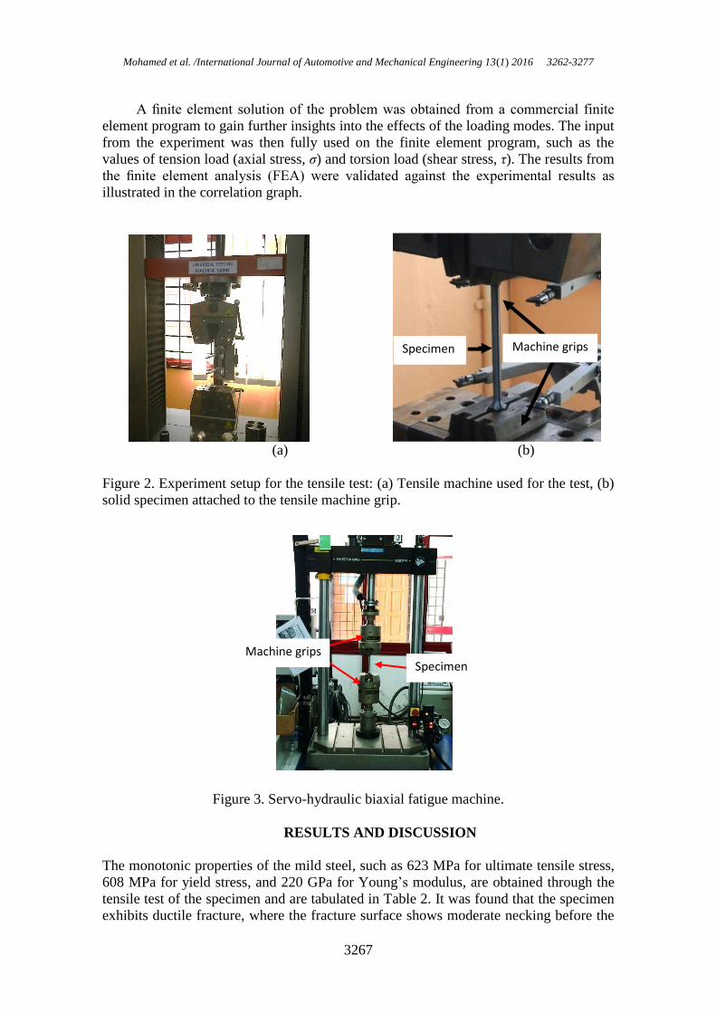
A finite element solution of the problem was obtained from a commercial finite

element program to gain further insights into the effects of the loading modes. The input

from the experiment was then fully used on the finite element program, such as the

values of tension load (axial stress, σ) and torsion load (shear stress, τ). The results from

the finite element analysis (FEA) were validated against the experimental results as

illustrated in the correlation graph.

(a) (b)

Figure 2. Experiment setup for the tensile test: (a) Tensile machine used for the test, (b)

solid specimen attached to the tensile machine grip.

Figure 3. Servo-hydraulic biaxial fatigue machine.

RESULTS AND DISCUSSION

The monotonic properties of the mild steel, such as 623 MPa for ultimate tensile stress,

608 MPa for yield stress, and 220 GPa for Young’s modulus, are obtained through the

tensile test of the specimen and are tabulated in Table 2. It was found that the specimen

exhibits ductile fracture, where the fracture surface shows moderate necking before the

Specimen Machine grips

Specimen Machine grips


3268

break which is shown in Figure 4. The nature of ductile fracture is associated with a

large amount of plastic deformation and occurs when the total stress (the sum of local

stress, flow stress and hydrostatic stress) exceeds the interface bond strength [20]. The

ultimate tensile strength is used as an indicator of a material limit stress at which the

input parameters for the cyclic test. The Young’s modulus is used to describe the elastic

properties of material in the strain–life curve. The fatigue life of the experiment is

shown in Table 3 for the five recorded values of equivalent stress from Eq. (6). The

fatigue life of the mild steel is in the range of 100 to 102 cycles. Values for the

experimental fatigue life are plotted in a log–log scale graph in Figure 5, which is

calculated using the equivalent von Mises strain using Eq. (7), because this approach

gives the same effect as a corresponding uniaxial strain state with the change to the

value of the combined multiaxial strain [21].

Figure 4. Necking fracture area of the specimen for tensile test.

Table 2. Experimentally determined monotonic properties of mild steel.

Properties Value

Ultimate tensile stress, σu 623 MPa

Yield stress, σy 608 MPa

Young’s modulus, E 220 GPa

Table 3. Fatigue life for constant biaxial loading.

Percentage of UTS value

(%)

Equivalent stress

(MPa)

Fatigue life

(cycle)

50

60

805

821

106

104

70 843 46

80 859 44

90 888 36

Fatigue Life Assessment

Fatigue life results from the experiment were collected. The fatigue life from the

simulations were calculated by using three different approaches, namely, Coffin–

Manson (CM), Smith–Watson–Topper (SWT), and Morrow (M), which are expressed

in Eqs. (1–3). The curve that represents the data in Figure 5 is called a strain–life curve


3269

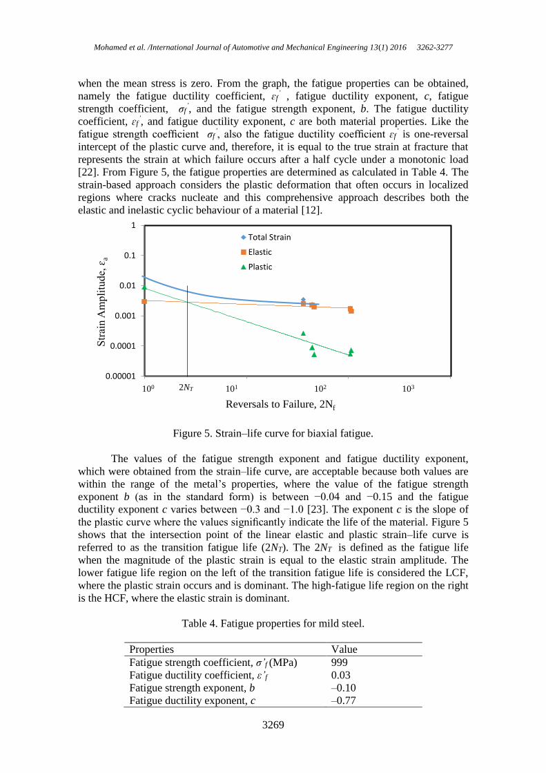
when the mean stress is zero. From the graph, the fatigue properties can be obtained,

namely the fatigue ductility coefficient, ɛf’ , fatigue ductility exponent, c, fatigue

strength coefficient, σf

’, and the fatigue strength exponent, b. The fatigue ductility

coefficient, ɛf’, and fatigue ductility exponent, c are both material properties. Like the

fatigue strength coefficient

σf’, also the fatigue ductility coefficient ɛf

’ is one-reversal

intercept of the plastic curve and, therefore, it is equal to the true strain at fracture that

represents the strain at which failure occurs after a half cycle under a monotonic load

[22]. From Figure 5, the fatigue properties are determined as calculated in Table 4. The

strain-based approach considers the plastic deformation that often occurs in localized

regions where cracks nucleate and this comprehensive approach describes both the

elastic and inelastic cyclic behaviour of a material [12].

Figure 5. Strain–life curve for biaxial fatigue.

The values of the fatigue strength exponent and fatigue ductility exponent,

which were obtained from the strain–life curve, are acceptable because both values are

within the range of the metal’s properties, where the value of the fatigue strength

exponent b (as in the standard form) is between −0.04 and −0.15 and the fatigue

ductility exponent c varies between −0.3 and −1.0 [23]. The exponent c is the slope of

the plastic curve where the values significantly indicate the life of the material. Figure 5

shows that the intersection point of the linear elastic and plastic strain–life curve is

referred to as the transition fatigue life (2NT). The 2NT is defined as the fatigue life

when the magnitude of the plastic strain is equal to the elastic strain amplitude. The

lower fatigue life region on the left of the transition fatigue life is considered the LCF,

where the plastic strain occurs and is dominant. The high-fatigue life region on the right

is the HCF, where the elastic strain is dominant.

Table 4. Fatigue properties for mild steel.

Properties Value

Fatigue strength coefficient, σ’f (MPa) 999

Fatigue ductility coefficient, ε’f 0.03

Fatigue strength exponent, b –0.10

Fatigue ductility exponent, c –0.77

0.00001

0.0001

0.001

0.01

0.1

1

1 10 100 1000

Str

ain A

mp

litu

de,

ɛa

Reversals to Failure, 2Nf

Total Strain

Elastic

Plastic

100 101 102 103 2NT


3270

Fatigue life was then estimated by using the CM, SWT, and Morrow models. The

equivalent strain data were plotted together in Figure 6. However, the consolidation

shows that many of the points are plotted within the factor of 2:1, whereas a few points

are located outside the correlation line. Thus, the experimental fatigue lives are

acceptable and accurate [24] . The test results indicated that the fatigue life decreased in

the experiment compared with the prediction life for the combined axial–torsion

loading. The combined data plotted in the graph clearly shows that most of the points

are within the error factor, while only a few points of 15% are located outside the line

correlation, so this agrees with the von Mises criterion for steel [25]. The fatigue life for

the three approaches is stated in Table 5. The experiment fatigue life is the closest to the

Coffin–Manson prediction approach. This is because, in considering the situation in

which the average stress value is zero, the Coffin–Manson approach provides accuracy

in the calculation.

Table 5. Total fatigue life for experiments and simulations under biaxial stress of the

mild steel.

Equivalent

stress (MPa)

Fatigue life (cycle)

Experiment Coffin–

Manson

Morrow SWT

805 106 78 47 70

821 104 41 27 38

843 46 24 16 22

859 44 15 11 14

888 36 5 4 5

Figure 6. Relationship between predicted and experimental fatigue.


3271

Figure 7. Mohr’s circle for a 3D state of stress under biaxial loading from ultimate

tensile stress (a) 0.5, (b) 0.6, (c) 0.7, (d) 0.8, and (e) 0.9 Su.

(b) (a)

(c) (d)

(e)

Principal Stress,

σ (MPa) Principal

Stress, σ

(MPa)

Principal Stress,

σ (MPa)

Principal Stress,

σ (MPa)

Principal

Stress, σ

(MPa)


3272

Principal Normal Stress and Maximum Shear Stress on Mohr’s Circle

The principal normal stresses and maximum shear stress on the inclined planes where

the loads were acting can be calculated by using Mohr’s circle. This graphical

representation is extremely useful because it enables the visualisation of the relationship

between normal and shear stresses acting on various inclined planes at a point in a

stressed body. Two of the circles lie inside the largest circle, and each circle is tangent

along the σ-axis to the other two, as shown in Figure 7. This result implies that the

allowable normal stress refers to the principal normal stress and that the allowable shear

stress refers to the absolute maximum shear stress. The allowable tensile normal stress

refers to principal stress 1 (σ1), where the load action is in tension. Furthermore, the

allowable compressive normal stress refers to principal stress 3 (σ3), which works in

compression. In this case, the principal stress 2 (σ2) is equal to zero because there is no

load acting in that direction. Hence, the maximum shear stress refers to the highest point

of the outer circle on the biggest Mohr’s circle, the same value that is given by the radii

of the circles. The trend expresses that increasing the load applied increases the values

of σ1 and τmax. It shows the opposite trend for the value of σ3. The values of the principal

stresses increase and decrease in the range of about 5%–7%, as shown in Figure 8 and

Table 6. The increments of the applied load tend to move the circle position to the right.

The force acting on the plane (red circle) creates a uniform normal stress on the cross-

sectional area of the specimen when tension load is applied to the tension plane, thus

affecting the increase of the σ1 value and τmax and decreasing the value of σ3 (green

circle) (Figure 9). The activated plane indicates that not only is there normal stress but

each stress is accompanied by shear stress.

Table 6. Normal stress and shear stress from the Mohr’s circle analysis.

Applied load Normal stress

1, σ1 (MPa)

Normal stress

2, σ2 (MPa)

Normal stress

3, σ3 (MPa)

Maximum

shear stress,

τmaks (MPa)

0.5σse 612 0 -300 456

0.6σse 648 0 -275 462

0.7σse 693 0 -257 474

0.8σse 724 0 -226 475

0.9σse 767 0 -206 486

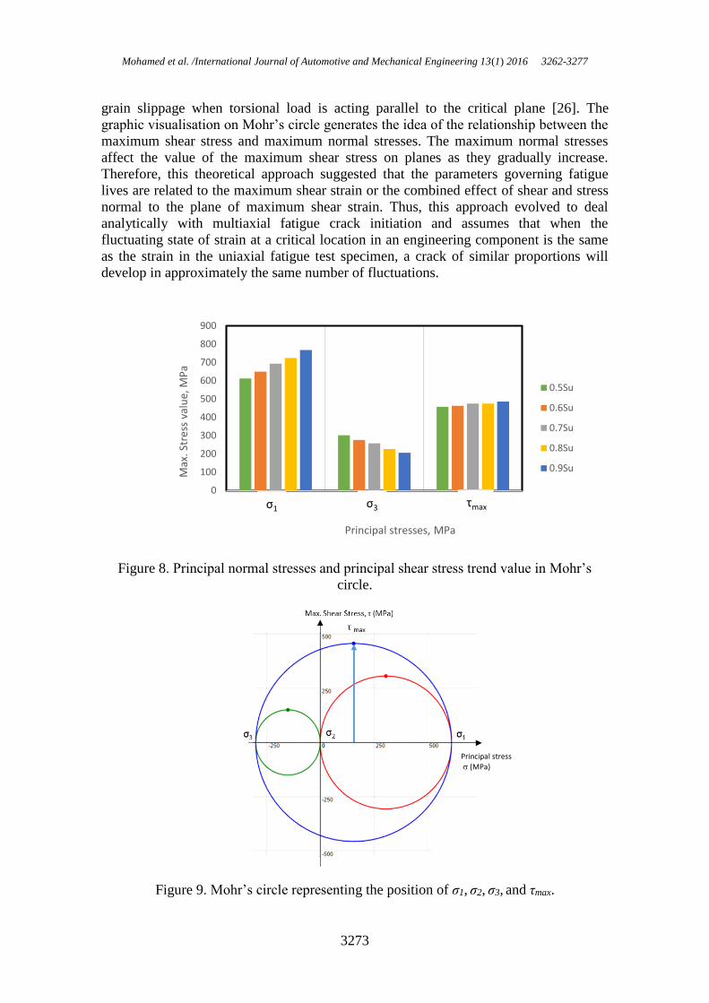
The results shown in Mohr’s circles clearly explain the different values and

trends given on each of the stresses involved (Figure 8). The graph explains that σ1

contributed significantly to fatigue failure. This result can be attributed to normal action

of the principal normal stress on crack propagation, whereas the maximum shear stress

was parallel to the crack plane. The observation indicates that cracks nucleate and grow

on certain planes (critical plane) depending on the material and loading conditions

(either maximum shear planes or maximum normal stress planes). Cracks as a result of

the tensile stress categorized as formed in Mode I were affected by the maximum

normal stress components. At this stage, the bonding strength of the structure is weak

because of stress acting perpendicular to the plane. Therefore, the driving force leads to

the nucleation of voids in the structure and then continues to crack growth, causing

premature failure. Shear cracks form at the plane of maximum shear stress, and the

process is failing in Mode II. In this case, the individual experiences the formation of


3273

grain slippage when torsional load is acting parallel to the critical plane [26]. The

graphic visualisation on Mohr’s circle generates the idea of the relationship between the

maximum shear stress and maximum normal stresses. The maximum normal stresses

affect the value of the maximum shear stress on planes as they gradually increase.

Therefore, this theoretical approach suggested that the parameters governing fatigue

lives are related to the maximum shear strain or the combined effect of shear and stress

normal to the plane of maximum shear strain. Thus, this approach evolved to deal

analytically with multiaxial fatigue crack initiation and assumes that when the

fluctuating state of strain at a critical location in an engineering component is the same

as the strain in the uniaxial fatigue test specimen, a crack of similar proportions will

develop in approximately the same number of fluctuations.

Figure 8. Principal normal stresses and principal shear stress trend value in Mohr’s

circle.

Figure 9. Mohr’s circle representing the position of σ1, σ2, σ3, and τmax.

0

100

200

300

400

500

600

700

800

900

σ1 σ3 τmax

Max

. Str

ess

valu

e, M

Pa

Principal stresses, MPa

0.5Su

0.6Su

0.7Su

0.8Su

0.9Su

σ1 σ3 τmax

Principal stress

(MPa)


3274

The behaviour of the biaxial fatigue is explained by the cyclic stress–strain

relationship. Figure 10 demonstrates the shape of the hysteresis loop for mild steel

under tension torsion loading. The hysteresis loop exhibits the elastic strain recovery as

the large size of the area underneath loading and unloading curves. The area enclosing

the hysteresis loop is equal to the amount of energy dissipated in the material upon the

loading and unloading processes. Thus, the behaviour tends to show cyclic hardening

with increasing Δσ/Δε [27]. When subjected to cyclic hardening, the process involved in

fatigue deformation is the twinning–detwinning process, which plays a dominant role at

the high strain amplitude. Dislocation slip dominates at the low strain amplitude. This

result indicates that axial loading is the main cause of failure (Figure 11). Stress

continually increases to drive the plastic deformation once the yield occurs.

Figure 10. Hysteresis loop for biaxial fatigue.

Figure 11. Correlation of shear stress and axial stress through material failure.

0.5Su 0.6Su 0.7Su 0.8Su 0.9Su

Ax

ial

Str

ess,

σ M

Pa

Shear Stress, τ MPa


3275

CONCLUSIONS

The strain–life curve for biaxial fatigue was plotted from the experiment results. The

fatigue properties for mild steel were obtained from the curve. A good correlation was

observed between the experimental fatigue life and predicted fatigue life. The behaviour

showed that the biaxial fatigue life decreases with increasing stress. Individual loading

in the biaxial fatigue provides a different impact on structure failure. The tension loads

work perpendicular to the crack plane and contribute to the opening of cracks. On the

contrary, shear stress acts in parellel yet has a small effect on crack growth. Finally, the

domain of the structure failure depends on the tension loads that are applied when

considering multiaxial fatigue. The normal stress obtained from the stress 0.5 Su, 0.6 Su,

0.7 Su, 0.8 Su and 0.9 Su is 612 MPa, 648 MPa, 693 MPa, 724 MPa and 767 MPa, while

the shear stress that is equivalent to the result of normal stress is 456 MPa, 462 MPa,

474 MPa, 475 MPa and 475 MPa. The increment of both stresses is in the range of 5%–

7%. Biaxial fatigue behaviour is then discussed with the stress–strain diagram of

relationships that form a cyclic hysteresis loop. The area within the hysteresis loop is

equivalent to the total energy released when the process of loading and unloading

occurs. The amount of energy produced by stress 0.5 Su, 0.6 Su, 0.7 Su, 0.8 Su and 0.9 Su

increases the number for each value of applied stress in the range 500 kJ/m3 to 605

kJ/m3, in which the lowest energy is produced by stress at 0.5 Su and the highest energy

is represented by the stress at 0.9 Su. Through this investigation, the ideas may provide

exposure and an overview on the characterization of biaxial fatigue loading. This result

is significant as a basic overview for the initial stage of design to improve the fatigue

life in normal operating loads for automotive components by knowing the maximum

normal and shear stress that the components can sustain.

ACKNOWLEDGEMENTS

The authors would like to express their gratitude to Universiti Kebangsaan Malaysia

through the fund of LRGS/2013/UPNM-UKM/DS/04 and the fund of

FRGS/2/2014/TK01/UKM/02/3 for supporting this research project.

REFERENCES

[1] Kamal M, Rahman M. Fatigue life estimation models: a state of the art.

International Journal of Automotive and Mechanical Engineering. 2014;9:1599.

[2] Itoh T, Sakane M, Ohsuga K. Multiaxial low cycle fatigue life under non-

proportional loading. International Journal of Pressure Vessels and Piping.

2013;110:50-6.

[3] Liu J, Li J, Zhang Z-p. A Three-Parameter Model for Predicting Fatigue Life of

Ductile Metals Under Constant Amplitude Multiaxial Loading. Journal of

materials engineering and performance. 2013;22:1161-9.

[4] Abdul Majid MS, Daud R, Afendi M, Amin NAM, Cheng EM, Gibson AG, et

al. Stress-Strain Response Modelling of Glass Fibre Reinforced Epoxy

Composite Pipes under Multiaxial Loadings. Journal of Mechanical Engineering

and Sciences. 2014;6:916-28.

[5] Kamal M, Rahman MM, Rahman AGA. Fatigue Life Evaluation of Suspension

Knuckle using Multibody Simulation Technique. Journal of Mechanical

Engineering and Sciences. 2012;3:291-300.


3276

[6] Shang D-G, Sun G-Q, Deng J, Yan C-L. Multiaxial fatigue damage parameter

and life prediction for medium-carbon steel based on the critical plane approach.

International Journal of Fatigue. 2007;29:2200-7.

[7] Araújo J, Dantas A, Castro F, Mamiya E, Ferreira J. On the characterization of

the critical plane with a simple and fast alternative measure of the shear stress

amplitude in multiaxial fatigue. International Journal of Fatigue. 2011;33:1092-

100.

[8] Golos KM, Debski DK, Debski MA. A stress-based fatigue criterion to assess

high-cycle fatigue under in-phase multiaxial loading conditions. Theoretical and

Applied Fracture Mechanics. 2014;73:3-8.

[9] Xu S-S, Nieto-Samaniego A, Alaniz-Álvarez S. 3D Mohr diagram to explain

reactivation of pre-existing planes due to changes in applied stresses.

International Symposium on In-Situ Rock Stress: International Society for Rock

Mechanics; 2010.

[10] Kamal M, Rahman MM. Dual-Criteria Method for Determining Critical Plane

Orientation for Multiaxial Fatigue Prediction Using a Genetic Algorithm.

International Journal of Automotive and Mechanical Engineering.

2015;11:2571-81.

[11] Biancolini M, Brutti C, Pennestri E, Valentini P. Dynamic, mechanical

efficiency, and fatigue analysis of the double Cardan homokinetic joint.

International Journal of Vehicle Design. 2003;32:231-49.

[12] Ince A, Glinka G. A modification of Morrow and Smith–Watson–Topper mean

stress correction models. Fatigue & Fracture of Engineering Materials &

Structures. 2011;34:854-67.

[13] Kamal M, Rahman M, Rahman A. Fatigue life evaluation of suspension knuckle

using multi body simulation technique. Journal of Mechanical Engineering and

Sciences. 2012;3:291-300.

[14] Yunoh MFM, Abdullah S, Saad MHM, Nopiah ZM, Nuawi MZ. Fatigue Feature

Extraction Analysis Based on a K-Means Clustering Approach. Journal of

Mechanical Engineering and Sciences. 2015;8:1275-82.

[15] Rahman M, Noor M, Bakar R, Maleque M, Ariffin A. Finite element based

fatigue life prediction of cylinder head for two-stroke linear engine using stress-

life approach. Journal of Applied Sciences. 2008;8:3316-27.

[16] Niesłony A, Böhm M. Mean stress effect correction using constant stress ratio

S–N curves. International journal of fatigue. 2013;52:49-56.

[17] Kwofie S, Chandler H. Low cycle fatigue under tensile mean stresses where

cyclic life extension occurs. International Journal of Fatigue. 2001;23:341-5.

[18] Lowisch G, Bomas H and Mayr P.Fatigue crack initiation and propagation in

ductile steels under multiaxial loading. Multiaxial and Fatigue Design, ESIS 21,

Mechanical Engineering Publication, London, 1996; 243-59.

[19] Zarroug N, Padmanabhan R, MacDonald B, Young P, Hashmi M. Mild steel

(En8) rod tests under combined tension–torsion loading. Journal of Materials

Processing Technology. 2003;143:807-13.

[20] Pradhan P, Robi P, Roy SK. Micro void coalescence of ductile fracture in mild

steel during tensile straining. Frattura ed Integrità Strutturale. 2012.

[21] Ion D, Lorand K, Mircea D, Karolv M. The equivalent stress concept in

multiaxial fatigue. Journal of Engineering Studies and Research. 2011;17:53-62.

[22] Milella PP. Fatigue and corrosion in metals: Springer Science & Business

Media; 2012.


3277

[23] Castillo E, Fernández-Canteli A, Pinto H, López-Aenlle M. A general regression

model for statistical analysis of strain–life fatigue data. Materials Letters.

2008;62:3639-42.

[24] Kim K, Chen X, Han C, Lee H. Estimation methods for fatigue properties of

steels under axial and torsional loading. International Journal of Fatigue.

2002;24:783-93.

[25] Mohammad M, Abdullah S, Jamaludin N, Innayatullah O. Predicting the fatigue

life of the SAE 1045 steel using an empirical Weibull-based model associated to

acoustic emission parameters. Materials & Design. 2014;54:1039-48.

[26] Stephens RI, Fatemi A, Stephens RR, Fuchs HO. Metal fatigue in engineering:

John Wiley & Sons; 2000.

[27] Landgraf R, Morrow J, Endo T. Determination of the cyclic stress-strain curve.

Journal of Malterials. 1969;4:176-88.

Documents

Characterization of the biaxial fatigue behaviour on ...ijame.ump.edu.my/images/Volume 13 Issue 1 June 2016/12_mohamed … · ... Cyclic hardening; maximum shear ... to that associated