Embed Size (px)
Citation preview
1
Sede Amministrativa: Università degli Studi di Padova
Dipartimento di: INGEGNERIA DELL’INFORMAZIONE (DEI)
___________________________________________________________________
SCUOLA DI DOTTORATO DI RICERCA IN: INGEGNERIA DELL’INFORMAZIONE
INDIRIZZO: SCIENZA E TECNOLOGIA DELL’INFORMAZIONE
CICLO: XXVII
CHARACTERIZATION OF PLASMONIC SURFACES FOR SENSING
APPLICATIONS
Direttore della Scuola: Ch.mo Prof. Matteo Bertocco
Coordinatore d’indirizzo: Ch.mo Prof. Carlo Ferrari
Supervisore: Ch.mo Prof. Alessandro Paccagnella
Dottorando: Mauro Perino

2

3
“From a long view of the history of mankind - seen from, say, ten thousand years from now -
there can be little doubt that the most significant event of the 19th century will be judged as
Maxwell's discovery of the laws of electrodynamics. The American Civil War will pale into
provincial insignificance in comparison with this important scientific event of the same decade”
Richard Phillips Feynman

4

5
Table of Contents:
Abstract (italiano) ......................................................................................................................... 7
Abstract (English).......................................................................................................................... 8
Introduction................................................................................................................................ 11
1 Surface Plasmon Polaritons ............................................... 15
1.1 Theory of Surface Plasmon Polaritons ........................................................... 15
1.2 Excitation of Surface Plasmon Polaritons ...................................................... 20
1.2.1 Flat Surfaces ........................................................................................... 21
1.2.2 Nanostructured surfaces ........................................................................ 23
1.3 Surface plasmon resonance sensors .............................................................. 25
1.3.1 Performances ......................................................................................... 25
1.3.2 Detection techniques ............................................................................. 28
1.3.3 Applications ........................................................................................... 30
2 Surfaces Simulation Methods ............................................ 33
2.1 Rigorous Coupled Wave Analysis Method ..................................................... 34
2.2 Chandezon method ........................................................................................ 39
2.3 Finite Element Method .................................................................................. 46
2.4 Vector model method .................................................................................... 50
3 Simulation Results ............................................................. 53
3.1 Nanostructured surfaces in conical mounting configuration......................... 53
3.1.1 Grating ................................................................................................... 53
3.1.2 Two-dimensional nanostructures .......................................................... 56
3.2 Kretschmann configuration ........................................................................... 59
3.2.1 Flat surfaces ........................................................................................... 60
3.2.2 Grating surfaces ..................................................................................... 61
3.3 Relationship between the Kretschmann and grating configurations ............ 63
3.4 Simulated sensitivity ...................................................................................... 68

6
3.4.1 Wavelength sensitivity ........................................................................... 69
3.4.2 Incident angle sensitivity ........................................................................ 72
3.4.3 Polarization sensitivity ........................................................................... 77
3.4.4 Azimuthal angle sensitivity ..................................................................... 80
4 Experimental Results ......................................................... 85
4.1 Experimental methods ................................................................................... 85
4.1.1 Conical mounting configuration bench .................................................. 85
4.1.2 Kretschmann configuration bench ......................................................... 89
4.1.3 Grating and flat surface, Atomic Force Microscope characterization .... 91
4.2 SPR Characterization ...................................................................................... 93
4.2.1 Grating, Ttot in conical mounting configuration ...................................... 93
4.2.2 Flat, R0 in Kretschmann configuration .................................................... 95
4.2.3 Grating, R0 in Kretschmann configuration .............................................. 96
4.3 Detection of bulk refractive index variations ................................................. 97
4.4 Detection of Alkanethiols Self Assembled Monolayers ............................... 103
4.4.1 Functionalization protocols .................................................................. 103
4.4.2 Incident angle sensitivity ...................................................................... 104
4.4.3 Azimuthal sensitivity ............................................................................ 104
4.5 Detection of an antibody layer ..................................................................... 109
4.5.1 Functionalization protocols .................................................................. 109
4.5.2 Incident angle sensitivity (Kretschmann configuration) ....................... 110
4.5.3 Azimuthal angle sensitivity ................................................................... 111
5 Conclusions................................................................................................................... 113
6 Acknowledgements ...................................................................................................... 115
7 Bibliography ................................................................................................................. 117
List of abbreviations and acronyms .......................................................................................... 125

7
Abstract (italiano) Durante il mio periodo di dottorato in Scienza e Tecnologia dell’Informazione l’attività di ricerca
principale è stata focalizzata sulla caratterizzazione, simulativa e sperimentale, dei plasmoni di
superficie.
I plasmoni di superficie sono onde elettromagnetiche evanescenti che si propagano
all’interfaccia tra un mezzo metallico ed un mezzo dielettrico. Il loro vettore d’onda è più elevato
rispetto a quello della luce nel mezzo dielettrico. Per poter quindi generare l’eccitazione si
devono utilizzare particolari tecniche di accoppiamento. I due metodi più diffusi sono
l’accoppiamento Kretschmann e l’accoppiamento tramite reticolo.
Una volta raggiunte le condizioni di accoppiamento dei plasmoni di superficie, si realizza il
fenomeno della risonanza plasmonica, la quale si manifesta attraverso brusche variazioni nelle
componenti della luce riflessa o trasmessa dalla superficie. Tipicamente si può registrare un
minimo della riflettanza in funzione dell’angolo di incidenza della luce sulla superficie. Esistono,
tuttavia, anche altre modalità per registrare e misurare queste risonanze, come ad esempio
monitorando intensità, polarizzazione o fase della luce trasmessa e riflessa dalla superficie, in
funzione della sua lunghezza d’onda o dei sui angoli di incidenza.
Le variazioni chimico/fisiche che avvengono all’interfaccia metallo/dielettrico, modificando la
costante di accoppiamento plasmonica, cambiano le condizioni di risonanza. Nel caso in cui le
variazioni all’interfaccia siano dovute ad un processo di riconoscimento molecolare è possibile
rilevare le molecole d’interesse valutando i cambiamenti della risonanza plasmonica, fornendo
così l’opportunità per l’implementazione di sensori specifici.
L’attività di dottorato è stata focalizzata innanzitutto sullo studio teorico del comportamento
della risonanza plasmonica, utilizzando varie tecniche di simulazione numerica: il metodo RCWA
(Rigorous Coupled Wave Analysis), Il metodo di Chandezon ed il metodo agli elementi finiti,
implementato tramite Comsol v3.5.
Ho poi affrontato lo studio, tramite simulazioni, delle risonanze di superficie in configurazione
Kretschmann, sia per interfacce metallo/dielettrico piane sia per interfacce nano-strutturate.
Considerando una configurazione conica, ho simulato le risonanze di superficie per nano-
strutture reticolari e per nano-strutture bi-dimensionali periodiche. Inoltre ho analizzato il
legame tra le modalità di accoppiamento grating e Kretschmann.
Tramite queste simulazioni mi è stato possibile valutare e studiare la sensibilità delle varie
risonanze plasmoniche alla variazione di indice di rifrazione, quando essa avviene all’interfaccia
metallo/dielettrico. È stato così possibile identificare un nuovo parametro per descrivere la
risonanza plasmonica e la sua sensibilità, ossia l’angolo azimutale, definito come l’angolo tra il
vettore del grating ed il piano di scattering della luce. Considerando questo particolare angolo, la
sensibilità del sensore può essere controllata con un’opportuna regolazione degli altri parametri
coinvolti nell’eccitazione plasmonica, consentendole di raggiungere valori molto elevati.
Successivamente, grazie all’utilizzo di due banchi, uno per la configurazione Kretschmann ed uno
per la misura di reticoli nano-strutturati in configurazione conica, ho realizzato delle campagne
8
di misure sperimentali. E’ stato così possibile confrontare i risultati sperimentali con le
simulazioni numeriche per le seguenti condizioni:
Interfaccia piana, configurazione Kretschmann
reticolo nano-strutturato, configurazione Kretschmann
reticolo nano-strutturato, configurazione conica
L’attività sperimentale si è particolarmente focalizzata sul reticolo nano-strutturato, sia per
l’innovativa modalità di caratterizzazione delle sue risonanze plasmoniche (valutazione del
segnale trasmesso in funzione dell’angolo di incidenza e dell’angolo azimutale), sia per l’elevata
sensibilità ottenuta valutando la variazione dell’angolo azimutale. La caratterizzazione è stata
effettuata sia per il reticolo esposto all’aria che per il reticolo immerso in un liquido (tipicamente
acqua).
Per poter verificare il comportamento della sensibilità azimutale ho variato l’indice di rifrazione
del liquido in contatto con la superficie utilizzando soluzioni miste di acqua e glicerolo. Inoltre,
tramite tecniche di funzionalizzazione della superficie, ovvero applicando delle molecole thiolate
che vengono adsorbite sulla parte metallica dell’interfaccia, mi è stato possibile variare le
costanti di accoppiamento plasmonico, in modo da verificare la capacità del dispositivo di
rilevare l’avvenuta creazione di uno strato molecolare sulla superficie. Inoltre ho positivamente
verificato la capacità di immobilizzare uno strato di anticorpi sulla superficie plasmonica.
Tutte le misure sperimentali che ho svolto in questa tesi sono state effettuate su sensori con
superfici piane o nano-strutturate prodotte dallo spin-off universitario Next Step Engineering,
con il quale ho collaborato durante il percorso di ricerca.
Abstract (English)
My research activity during the Ph. D. period has been focused on the simulation and the
experimental characterization of Surface Plasmon Polaritons (SPP).
Surface Plasmon Polaritons are evanescent electromagnetic waves that propagate along a
metal/dielectric interface. Since their excitation momentum is higher than that of the photons
inside the dielectric medium, they cannot be excited just by lighting the interface, but they need
some particular coupling configurations. Among all the possible configurations the Kretschmann
and the grating are those largely widespread.
When the SPP coupling conditions are reached, abrupt changes of some components of the light
reflected or transmitted at the metal/dielectric interface appear. Usually this resonances are
characterized by a minimum of the reflectance acquired as a function of the incident angle or
light wavelength. Several experimental methods are available to detect these SPP resonances,
for instance by monitoring the light intensity, its polarization or its phase.
Changes in the physical conditions of the metal/dielectric interface produce some changes of the
SPP coupling constant, and consequently a shift in the resonance position. If these changes

9
derive from a molecular detection process, it is possible to correlate the presence of the target
molecules to the resonance variations, thus obtaining a dedicated SPP sensor.
I focused the first part of my Ph.D. activity on the simulation of SPP resonances by using several
numerical techniques, such as the Rigorous Coupled Wave Analysis method, the Chandezon
method, and the Finite Element Method implemented through Comsol v3.5.
I simulated the SPP resonance in the Kretschmann coupling configuration for plane and nano-
grating structured metal/dielectric interfaces. Afterward, I calculated the SPP resonance
behaviour for grating and bi-dimensional periodic structures lighted in the conical configuration.
Furthermore, I analysed the correlations between the grating coupling method and the
Kretschamann coupling method.
Through all these simulations, I studied the sensitivity of the different SPP resonances to the
refractive index variation of the dielectric in contact with the metal. In this way, I was able to
find a new parameter suitable for describing the SPP resonance, i.e., the azimuthal angle. By
considering this particular angle, the sensitivity of the SPP resonances could be properly set
according to the experimental needs and, even more important, noticeably increased to high
values.
Experimentally I used two opto-electronic benches, one for the Kretschmann configuration and
one for the conical mounting configuration. I have performed experimental measurements, in
order to compare the experimental data with the simulations. In particular the following
conditions were tested:
Plane interface, Kretschmann configuration
Nanostructured grating, Kretschmann configuration
Nanostructured grating, Conical configuration
I focused my attention on the nano-structured grating in conical mounting configuration. I found
an innovative way to characterize its SPP resonances, by measuring the transmitted signal as a
function of the incident and azimuthal angles. The transmittance and the azimuthal sensitivities
were characterized with the gratings in both air and water.
In order to study the experimental azimuthal sensitivity, I changed the liquid refractive index in
contact with the grating by using different water/glycerol solutions. Moreover, I functionalized
the surface by using thiolated molecules that form Self Assembled Monolayer onto the metallic
layer. In this way, I was able to change the SPP coupling constants and detect the corresponding
azimuthal resonance shifts. I also detected the immobilization of an antibody layer onto the
metallic surface of the plasmonic interface.
All the devices I used in the experimental measurements were produced by the University spin
off Next Step Engineering.

10

11
Introduction
In the last three decades we witness to a growing interest in the biosensor field since methods
for fast accurate and reliable detection of analytes, such as biological molecules, pathogens,
toxins, and chemicals, are highly desired especially for applications such as medical diagnostic,
drug discovery, food safety and environmental monitoring.
Among all the possible sensors types, one attracts more interest, i.e. the affinity sensor. This
sensor is characterized by the presence of a molecular recognition element, which is able to
selectively bind a target analyte, affecting the sensors output. Affinity sensor could be based on
different transducing principles. They could be summarized in electrochemical, piezoelectric,
fluorescence, and optical sensors.
Among the optical transducing techniques, Surface Plasmon Resonance (SPR) achieved, over the
years, a growing use and interest. This technique exploits the excitation of Surface Plasmon
Polaritons (SPP) which are charge density waves travelling along a metal/dielectric interface. The
electric field associated with these waves decays exponentially in the direction perpendicular to
the propagation one. Most of the energy is then confined to the metal surface which explains
the remarkable sensitivity of SPR to changes in optical parameters at the metal/dielectric
interface.
Even if the early pioneering works on the SPP excitation through the Total Internal Reflection
(TIR) method dates back to the ‘60s, and the first applications to gas sensing and organic
monolayer assemblies detection appears between the ‘70s and ‘80s, the interest in this research
field is still considerably high and involves different groups all around the world. The main
features currently under improvement regard three main themes: reaching high throughput
analysis, enhancing the method sensitivity, and simplifying the SPP coupling scheme.
Since the SPPs momentum is greater than the light one in the dielectric medium, it is not
possible to excite them by simply lighting the metal/dielectric interface. In order to overcome
this problem different coupling configurations techniques were developed over the years. The
most used one is the Kretschmann configuration, where the light passes through an high
refraction index prism increasing in this way its incident momentum and allowing its coupling
with the SPPs. A similar method where the increasing in the light momentum is performed
taking advantage of an high refractive index medium is the waveguide one. The last main
method is called Grating Coupling SPR (GCSPR). In this configuration the difference between SPP
momentum and the light one is provide by exploiting the grating periodic momentum.
Even if the fabrication of a nanostructured surface is more challenging respect to the fabrication
of a flat surface required in the Kretschmann configurations, GCSPR configuration has one more
degrees of freedom i.e. the azimuthal angle (𝜙). 𝜙 is defined as the angle between the light
scattering plane and the grating momentum.
In this work we will analyse, by means of simulations, how 𝜙 affects the SPR excitation in one-
dimensional and two-dimensional periodic structures. Then by using a silver unidimensional

12
grating, provided by Next Step Engineering s.r.l., we will prove that the sensitivity of the method
could be enhanced by a factor of 20 respect to the Kretschmann configuration. We will also
consider the Figure of Merit (FOM) of this detection method and we will compare it to the
Kretschmann one.
The work is organized as follow:
Chapter 1 Surface Plasmon Polaritons. First we derive the expression for the SPP momentum by
using the Maxwell’s equations, supposing that the electromagnetic wave is confined at the
metal/dielectric interface and propagates along the surface. Then we analyse the SPP
polarization mode, propagation length, and its penetration depth. Furthermore we illustrate
what happens to these parameters if different metals are used in the interface. Then we
introduce the Kretschmann and the Grating coupling configuration methods. Finally we describe
the main feature of a SPR sensing system; we illustrate the main analyte detection method and
some applications of these technologies.
Chapter 2 Surface Simulation methods. In this chapter we depict three different simulation
methods that could be used to simulate the light diffracted by a periodical structured surface.
The first method we describe is the Rigorous Coupled Wave Analysis (RCWA). The second one is
the differential or Chandezon Method (CM). The last one is the Finite Element Method (FEM)
implemented through Comsol Multiphysics® version 3.5a. We use these methods to calculate
the diffraction efficiencies of a unidimensional grating in conical mounting configuration with
null azimuthal angle. The simulation results will be compared as well as the pros and cons of the
methods. Finally we generalize the simpler vector model method in order to apply it to the
calculations of the resonance in the two dimensional case.
Chapter 3 Simulation Results. In this chapter the grating total transmittance Ttot and zero order
reflectance R0 for the grating in conical mounting configuration will be simulated through the
RCWA method. Moreover we perform the same study by using bidimensional periodic structures
simulated through the FEM method. In both cases the resonances we found are well reproduced
by the vector model calculations. After this we simulate the response of a flat and
nanostructured surface lighted in the Kretschmann configurations. We also depict the link
between the Kretschmann and grating configuration when the SPP are excited. Finally the
sensitivity for both configurations are extensively studied through RCWA method. For the
Kretschmann configuration we analyse the incident angle and wavelength sensitivity meanwhile
for the grating configuration we also analyse the polarization and the azimuthal angle sensitivity.
Finally we describe in detail this new sensing method i.e. the azimuthal one, and we notice that
the sensitivity enhancement obtained is due to an almost parabolic shape of the plasmonic
resonance.
Chapter 4 Experimental Results. In this chapter we describe the optical benches we used to
evaluate the SPR in grating and Kretschmann configurations and a brief description of the
developed software will be reported. After this we show our experimental results regarding the
characterization of the Grating transmittance. We also report the order zero reflectance in the
Kretschmann configurations we found by using flat and unidimensional grating surfaces. Then
we characterize the sensitivity and FOM of the azimuthal detection method by changing the
buffer refractive index. We achieve this goals by using a custom microfluidic cell where different

13
glycerol/water solutions were flushed. We also check the ability of the method to detect the
presence of Self Assmbled Monlayer (SAM) of different thickness and we monitor the adsorption
kinetic of these molecules onto the silver metal surface. Finally, we compare the resonance
shifts caused by the immobilization of an antibody layer onto the silver flat and nanostructured
surfaces. The flat one are evaluated in the Kretschmann configurations meanwhile the
nanostructured one are measured by using the azimuthal method.

14

15
1 Surface Plasmon Polaritons
The first observation of Surface Plasmon Polaritons was performed by Wood [1] in 1902, who
reported anomalies in the spectrum of light diffracted on a metallic diffraction grating. But only
in 1941 Fano [2] proved that these anomalies are associated with the excitation of
electromagnetic surface waves on the surface of the diffraction grating. Later, in 1968, the work
of Otto [3] demonstrated that the drop in reflectivity in the attenuated total reflection method is
due to the excitation of SPPs. In the same year, Kretschmann and Raether [4] observed
excitation of SPPs in another configuration of the attenuated total reflection method. These
pioneering works established a convenient method for the excitation and investigation of SPP,
before modern nanofabrication technique allowed nanostructured gratings realization.
The first application of the SPR as a sensing tool was performed in 1974 by Reather. He
monitored the surface roughness of thin films [5].A few years later in 1977 Gordon detect a SPR
shift induced by the formation of an organic monolayer films onto the metallic layer [6]. Later in
1980, the group headed by Lundstrom reported the detection of gaseous analyte and
biomolecules and stared the new era of this label free techniques [7], [8]. Starting from these
pioneering works, a lot of studies have been done in order to improve both the excitation and
detection method of the plasmonic resonance as well as its sensitivity, resolution, and reliability.
Thanks to all these efforts SPR sensors are currently used in the analytical chemistry, material
science and biological fields. The great impact of this field is also attested by several reviews and
books [9]–[17] that describe the advance in the SPR sensor as well as the existence of
commercial instruments already available since the early ‘90s [18], [19].
In this chapter we will describe the main features of SPP starting from Maxwell’s equations. We
will derive the SPP dispersion law, which shows the typical non radiative character of these
surface waves. The evanescent nature of SPPs will be then highlighted together with their
surface propagation characteristics. We will then describe how to excite SPP by means of light.
Finally we will introduce some basic features of a biosensor device.
1.1 Theory of Surface Plasmon Polaritons
In order to achieve the condition for the SPP wave excitation we can start from Maxwell’s
equations in a continuous media without charge or current sources [15]:
∇𝑫 = 0 (1.1)
∇ × 𝑬 = −𝜕𝑩
𝜕𝑡 (1.2)
∇𝑩 = 0 (1.3)
𝛻 ×𝑯 = 𝜕𝑫
𝜕𝑡 (1.4)
We considered also these constitutive relations:
𝑫 = ε(𝒓)𝑬 (1.5) 𝑩 = μ(𝒓)𝑯 (1.6) where ε(𝒓) = 휀0 휀(𝒓) and, μ(𝒓) = 𝜇0 𝜇(𝒓), 휀, 𝜇 are respectively the relative dielectric
permittivity and the relative magnetic permeability of the medium meanwhile 휀0, 𝜇0 refers to

16
their values in vacuum, respectively. In this specific case, since we are interested in study time
harmonic wave propagation, the fields can be written as follow:
𝑬(𝑥, 𝑦, 𝑧, 𝑡) = 𝑬(𝑥, 𝑦, 𝑧)𝑒−𝑖𝜔𝑡 (1.7) 𝑯(𝑥, 𝑦, 𝑧, 𝑡) = 𝑯(𝑥, 𝑦, 𝑧)𝑒−𝑖𝜔𝑡 (1.8) For simplicity and practical purposes (since we will use Silver as metal) we will consider only non-
magnetic material. This implies that 𝜇 =1 in all our domains.
Taking the curl of (1.2) and using (1.4) and (1.2) we obtain this equation:
∇2𝑬 − ε(𝒓)μ𝜕2𝑬
𝜕𝑡2= ∇(−
1
ε(𝒓)𝑬 ∙ ∇ε(𝒓)) (1.9)
In a similar way, for the magnetic field:
∇2𝑯− ε(𝒓)μ𝜕2𝑯
𝜕𝑡2= (∇ × 𝐇) × (
∇ε(𝒓)
ε(𝒓)) (1.10)
Figure 1.1 Surface Plasmon Polaritons fields at the metal/dielectric interface.
Figure 1.1 schematically shows the system under analysis. We have a metal/dielectric interface
along the 𝑧=0 plane. The uniform metal region is confined in the 𝑧<0 region meanwhile the
uniform dielectric one is defined by the 𝑧>0 region. In each one of these two regions the value of
the dielectric permittivity is constant and uniform therefore in equations 1.9 and 1.10 can be
simplified becoming two typical Helmholtz equations:
𝛻2𝑬+ 휀𝑘02𝑬 = 0 (1.11)
𝛻2𝑯+ 휀𝑘02𝑯 = 0 (1.12)
where we have extracted the time harmonic propagation term and define 𝑘0 = 𝜔 𝑐⁄ .
Since we want the wave to be guided along the interface, we can assume that the wave is
travelling in the 𝑥-direction since the system is symmetric for 𝑧-axis rotation. Finally taking into
account that the system is also symmetric for 𝑦-axis translations we can assume that the general
form of the magnetic fields is described by:
𝑬(𝑥, 𝑦, 𝑧) = 𝑬(𝑧)𝑒𝑖𝑘𝑥𝑥 𝑯(𝑥, 𝑦, 𝑧) = 𝑯(𝑧)𝑒𝑖𝑘𝑥𝑥
(1.13)
17
Applying this field assumptions into the Helmholtz equations (1.11) and (1.12) we obtain:
𝜕2𝑯(𝑧)
𝜕𝑧2+ (휀𝑘0
2 − 𝑘𝑥2)𝑯(𝑧) = 0 (1.14)
𝜕2𝑬(𝑧)
𝜕𝑧2+ (휀𝑘0
2 − 𝑘𝑥2)𝑬(𝑧) = 0 (1.15)
These equations are the starting point for the study of electromagnetic modes in waveguides,
and more specifically for the analysis of SPP’ dispersion relation.
If we try to solve the above equations with the constraints coming from the Maxwell equations
1.2 and 1.4 we will find two independent solutions: the Transverse Magnetic (TM) propagation
mode, where only the 𝑦-component of magnetic field is present, and the Transverse Electric (TE)
propagation mode where only the y-component of electric field is present.
Both the dielectric and metallic medium can be described by a dielectric constant 휀𝑑 = 𝜖𝑑′ + 𝑖𝜖𝑑
′′
and 휀𝑚 = 𝜖𝑚′ + 𝑖𝜖𝑚
′′ , respectively. As we can see in this case we separate the real and imaginary
part of the dielectric constant. Now with these definition we can write the matching conditions
at the interface:
𝑬𝒅∥ = 𝑬𝒎
∥
휀𝑑𝑬𝒅⊥ = 휀𝑚𝑬𝒎
⊥ (1.16)
𝑯𝒅∥ = 𝑯𝒎
∥
𝜇𝑑𝑯𝒅⊥ = 𝜇𝑚𝑯𝒎
⊥ (1.17)
If we assume that a possible solution for the Maxwell’s equations in the TM mode has this form
𝑯𝑗 = (0,𝐻𝑗
𝑦, 0) 𝑒𝑖(𝑘𝑥,𝑗𝑥±𝑘𝑧,𝑗𝑧)
𝑬𝑗 = (𝐸𝑗𝑥 , 0, 𝐸𝑗
𝑧) 𝑒𝑖(𝑘𝑥,𝑗𝑥±𝑘𝑧,𝑗𝑧) (1.18)
Where j stands for dielectric (d) or metal (m) part of the wave guide.
In this case if we want to find a solution confined at the interface we have to assume 𝑘𝑧,𝑗 purely
imaginary and so we have to take the plus sign if z > 0 and the minus sign for z < 0 .
Immediately the boundary conditions 1.16 and 1.17 implies that
𝑘𝑥,𝑑 = 𝑘𝑥,𝑚 = 𝑘𝑥 (1.19) Inserting these fields in equation 1.14 we obtain the following algebraic relations:
𝑘𝑧,𝑑2 = 𝑘𝑥
2 − 𝑘02휀𝑑
𝑘𝑧,𝑚2 = 𝑘𝑥
2 − 𝑘02휀𝑚
(1.20)
Taking the curl relationship (1.4) for the TM case we found other conditions that has to be
satisfied

18
𝛁 ×𝑯𝑗 = (
∓𝐻𝑗𝑦𝑖𝑘𝑧,𝑗𝑒
𝑖(𝑘𝑥𝑥±𝑘𝑧,𝑗𝑧−𝜔𝑡)
0𝐻𝑗𝑦𝑖𝑘𝑥𝑒
𝑖(𝑘𝑥𝑥±𝑘𝑧,𝑗𝑧−𝜔𝑡)) = 휀𝑗
𝜕𝑬
𝜕𝑡
= (
−𝑖휀𝑗𝜔𝐸𝑗𝑥𝑒𝑖(𝑘𝑥𝑥±𝑘𝑧,𝑗𝑧−𝜔𝑡)
0−𝑖휀𝑗𝜔𝐸𝑗
𝑧𝑒𝑖(𝑘𝑥𝑥±𝑘𝑧,𝑗𝑧−𝜔𝑡))
(1.21)
Considering the 𝑥-component and applying the boundary conditions 1.16 and 1.17 we obtain
the system:
{
𝑘𝑧,𝑑𝜖𝑑
𝐻𝑑𝑦+𝑘𝑧,𝑚𝜖𝑚
𝐻𝑚𝑦= 0
𝐻𝑑𝑦− 𝐻𝑚
𝑦= 0
(1.22)
Which admits solution only if its determinant vanishes:
𝑘𝑧,𝑑휀𝑑
+𝑘𝑧,𝑚휀𝑚
= 0 (1.23)
If we now consider the case 𝜖𝑑′′ ≈ 𝜖𝑚
′′ ≈ 0 we can see that in order to solve the equation the
metallic nature of the lower part of the wave guide is crucial for the existence of surface waves.
In fact for a metallic material 𝑅𝑒(휀𝑚) < 0 hence 1.23 has solution.
Inserting this equation into (1.20) we obtain the Surface Plasmon Polaritons dispersion relation
𝑘𝑥 = 𝜔
𝑐√𝜖𝑑′ 𝜖𝑚
′
𝜖𝑑′ + 𝜖𝑚
′ (1.24)
SPP can exist only if we consider the incident light in TM mode. If the TE mode is considered the
previous calculations get the following equation instead of the 1.23:
(𝑘𝑧,𝑑 + 𝑘𝑧,𝑚)𝐸𝑗𝑦= 0 (1.25)
But in order to have a confined solution Re[𝑘𝑧,𝑗] = 0 and Im[𝑘𝑧,𝑗] > 0, this implies that the
only solution for equations 1.25 is 𝐸𝑗𝑦= 0; hence no SPP propagates in TE mode.
We will now analyse the propagation length and the penetration depth of the SPPs. The
propagation length can be derived by considering the SPP propagation constant we found in
1.24. Taking into account the complete metal dielectric constant the modulus of its real part is
much larger than its imaginary part |𝜖𝑚′ | ≫ 𝜖𝑚
′′ and the expression can be developed in a Taylor
series:
𝑘𝑥 = 𝛽 = 𝛽′ + 𝑖𝛽′′ =
𝜔
𝑐√𝜖𝑑′ 𝜖𝑚
′
𝜖𝑑′ + 𝜖𝑚
′ + 𝑖𝜖𝑚′′
2(𝜖𝑚′ )2
𝜔
𝑐(𝜖𝑑′ 𝜖𝑚
′
𝜖𝑑′ + 𝜖𝑚
′ )
32⁄
(1.26)
The imaginary part of the propagation constant represents the SPP wave attenuation by the
metal adsorption. This Implies that the field intensity decays with a characteristic length of
𝐿 = 1 2𝛽′′⁄ .
19
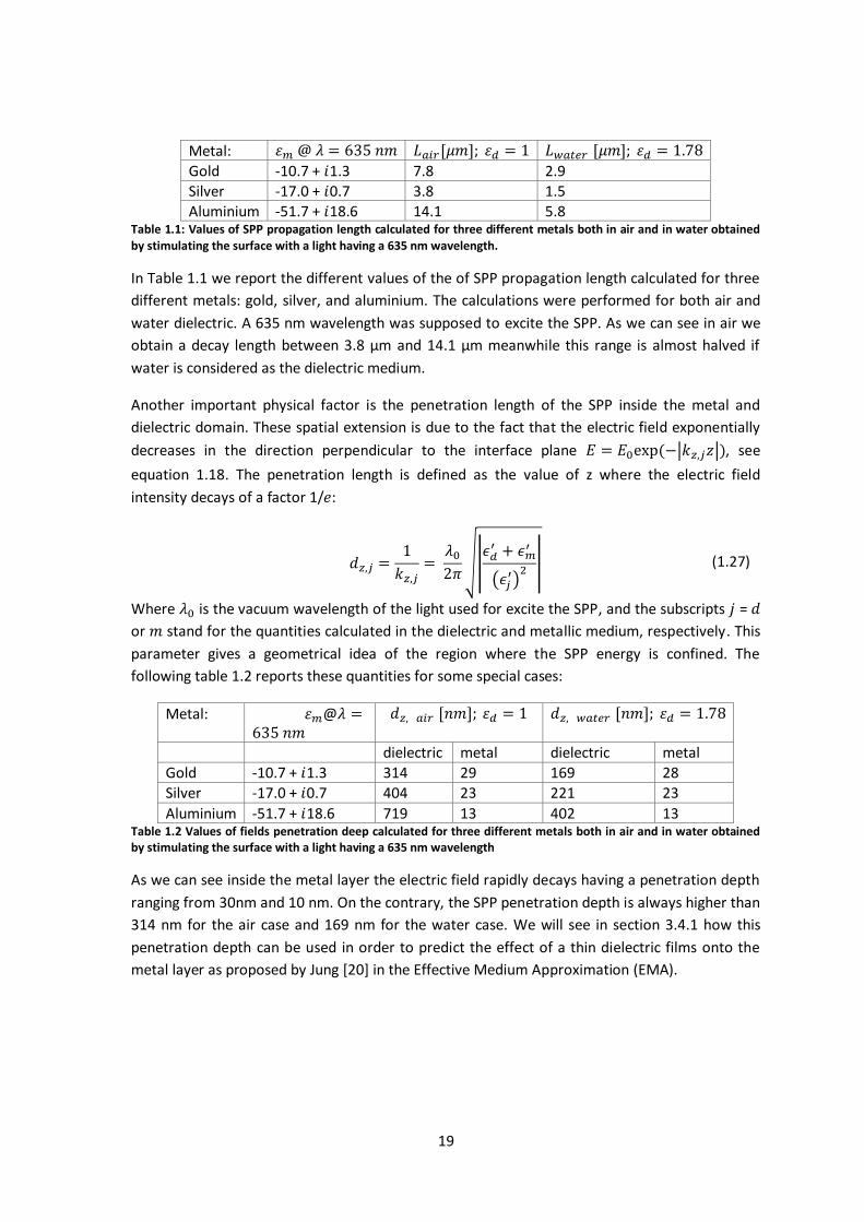
Metal: 휀𝑚 @ 𝜆 = 635 𝑛𝑚 𝐿𝑎𝑖𝑟[𝜇𝑚]; 휀𝑑 = 1 𝐿𝑤𝑎𝑡𝑒𝑟 [𝜇𝑚]; 휀𝑑 = 1.78
Gold -10.7 + 𝑖1.3 7.8 2.9
Silver -17.0 + 𝑖0.7 3.8 1.5
Aluminium -51.7 + 𝑖18.6 14.1 5.8 Table 1.1: Values of SPP propagation length calculated for three different metals both in air and in water obtained
by stimulating the surface with a light having a 635 nm wavelength.
In Table 1.1 we report the different values of the of SPP propagation length calculated for three
different metals: gold, silver, and aluminium. The calculations were performed for both air and
water dielectric. A 635 nm wavelength was supposed to excite the SPP. As we can see in air we
obtain a decay length between 3.8 μm and 14.1 μm meanwhile this range is almost halved if
water is considered as the dielectric medium.
Another important physical factor is the penetration length of the SPP inside the metal and
dielectric domain. These spatial extension is due to the fact that the electric field exponentially
decreases in the direction perpendicular to the interface plane 𝐸 = 𝐸0exp (−|𝑘𝑧,𝑗𝑧|), see
equation 1.18. The penetration length is defined as the value of z where the electric field
intensity decays of a factor 1/𝑒:
𝑑𝑧,𝑗 =1
𝑘𝑧,𝑗= 𝜆02𝜋√|𝜖𝑑′ + 𝜖𝑚
′
(𝜖𝑗′)2 | (1.27)
Where 𝜆0 is the vacuum wavelength of the light used for excite the SPP, and the subscripts 𝑗 = 𝑑
or 𝑚 stand for the quantities calculated in the dielectric and metallic medium, respectively. This
parameter gives a geometrical idea of the region where the SPP energy is confined. The
following table 1.2 reports these quantities for some special cases:
Metal: 휀𝑚@𝜆 =635 𝑛𝑚
𝑑𝑧, 𝑎𝑖𝑟 [𝑛𝑚]; 휀𝑑 = 1 𝑑𝑧, 𝑤𝑎𝑡𝑒𝑟 [𝑛𝑚]; 휀𝑑 = 1.78
dielectric metal dielectric metal
Gold -10.7 + 𝑖1.3 314 29 169 28
Silver -17.0 + 𝑖0.7 404 23 221 23
Aluminium -51.7 + 𝑖18.6 719 13 402 13 Table 1.2 Values of fields penetration deep calculated for three different metals both in air and in water obtained by stimulating the surface with a light having a 635 nm wavelength
As we can see inside the metal layer the electric field rapidly decays having a penetration depth
ranging from 30nm and 10 nm. On the contrary, the SPP penetration depth is always higher than
314 nm for the air case and 169 nm for the water case. We will see in section 3.4.1 how this
penetration depth can be used in order to predict the effect of a thin dielectric films onto the
metal layer as proposed by Jung [20] in the Effective Medium Approximation (EMA).

20
1.2 Excitation of Surface Plasmon Polaritons
In the previous sections we saw how to retrieve the SPP coupling constant but we did not
explain how to excite these electromagnetic guided modes. The excitation problems arise from
the fact that the light momentum in the dielectric is always lower than the SPP one, hence these
modes cannot be excite just by lighting the metal/dielectric interface.
In order to calculate the SPP dispersion relation an expression for the metal dielectric constant
has to be found. The simpler model for its the description is the plasma model. In this model the
free electrons of the metal are described as a gas of free electron that moves around a fixed
background of positive ion cores. The effect of the metallic lattice influences this model by
modifying the effective electron mass used and its validity extends until the lowest visible
frequencies. Below these wavelengths some interactions between the atom bounded electrons
and the light appear. We can consider that the electron gas responds to an applied electric field
following the sequent equation:
𝑚�̈� = −𝑚𝛾�̇� − 𝑒𝐄 (1.28) Where 𝒙 is the displacement from the equilibrium position, 𝛾 represents a damping
contribution, 𝑚 and 𝑒 are the electron effective mass and charge.
Assuming now an harmonic time dependency the equation 1.28 can be algebraic solved and the
displacement becomes:
𝒙(𝑡) =𝑒
𝑚(𝜔2 + 𝑖𝛾𝜔)𝐄(𝑡) (1.29)
Subsequently the polarization of the metal atoms becomes:
𝐏 = −𝑒𝑛𝒙 = −𝑛𝑒2
𝑚(𝜔2 + 𝑖𝛾𝜔) 𝐄 (1.30)
Where 𝑛 is the density of the free electrons.
Relating this polarization filed with the relative dielectric constant, we obtain:
휀(𝜔) = 1 − 𝜔𝑝2
𝜔2 + 𝑖𝛾𝜔 (1.31)
In this equation 𝜔𝑝 = 𝑛𝑒2
𝜖0𝑚 is the plasma frequency for the free electron gas and it is related to
the frequency of the longitudinal oscillations of the free electron gas.
The dielectric function can be divided into its real and imaginary part as follow:
𝜖′(𝜔) = 1 − 𝜔𝑝2𝜏2
1 +𝜔2𝜏2; 𝜖′′(𝜔) =
𝜔𝑝2𝜏
𝜔(1 + 𝜔2𝜏2) (1.31)
Here 𝜏 = 1 𝛾⁄ represents the time occurring between dumping collisions, and it is known as the
relaxation time; 𝛾 represents therefore the collision frequency.
Typical value for gold are 𝜔𝑝 = 12.1 × 10¹⁵ sec-1 (corresponding to a photon of 8 eV or 155
nm) and 𝜏 = 2.7 × 10⁻¹⁴ sec (corresponding to a photon of 25 meV or 49 μm if the
corresponding frequency 𝛾 is considered) [21].

21
If we consider 𝜔𝜏 ≫ 1 for (635 nm 𝜔 ~ 3 1015 Hz ) the damping is negligible and the dielectric
function is predominantly real:
𝜖(𝜔) = 1 − 𝜔𝑝2
𝜔2 (1.32)
Inserting the above expression for the metal dielectric function in the SPP momentum (eq 1.24)
we obtain the dispersion curves plotted in figure 1.2.
Figure 1.2 dispersion curves for the SPP propagating between air and a metal having the dielectric constant obtained from the plasma model (blue curve) and the light one in air (red curves).
We see that the dispersion curve of a SPP lies always on the right side of the dispersion relation
of light in vacuum. This implies that SPP cannot be directly excited by lighting the surface but
and additional momentum to the incoming photon must be added.
The coupling of the SPP at a metal dielectric interface is substantially determined by the
morphology of the metal dielectric interface. If the surface is flat the coupling method requires
to enhance the momentum of the coupling photon. Meanwhile if the surface is nanostructured
the photon momentum is enhanced by exploiting the grating momentum. We will describe in
detail the two cases in the following section.
1.2.1 Flat Surfaces
The most used method for the excitation of SPP along a flat metal/dielectric interface is the
Attenuated Total Internal Reflection (ATR). A typical scheme for ATR method is a three layers
system consisting on a thin metal film sandwiched between two dielectric media, for instance a
glass prism and air or water, with their dielectric constant respectively 𝜖𝑝, 𝜖𝑑 where the relation
𝜖𝑝 > 𝜖𝑑 must be satisfied. The 𝑥-component of the light momentum on the metal/glass
interface is 𝑘𝑥 = 𝑘0√𝜖𝑝 sin𝜃 where 𝜃 is the incident angle. This momentum is not sufficient to
excite SPP at the metal/glass interface. Nevertheless if we are in Total Internal Reflection (TIR)
condition an evanescent wave propagates parallel to the glass interface and if the metal film has
the correct thickness (~50 nm) this wave excite the SPP at the metal/air interface
In this case the condition that must be satisfied is:
0 1 2 3 4 5 60
0.2
0.4
0.6
0.8
1
1.2
1.4
SPP dispersion curve
kxc/
p
/p
SPP dispersion curve
air dispersion curve

22
𝑘0√𝜖𝑝 sin 𝜗 = 𝑘0√휀𝑑휀𝑚
휀𝑑 + 휀𝑚 (1.33)
This relation tells us that there is a cross point between the curve of light dispersion in prism and
the curve of SPP dispersion at metal/air interface.
This idea has been implemented into two different excitation configurations: the Kretschmann
and the Otto one[3], [4].
Figure 1.3 a) Schematic of the Kretschmann coupling method b) dispersion curves of the methods
In figure 1.3a we report the typical Kretschmann configuration. The light incoming from the
prism impinges the metal films with an angle 𝜃. Then when the correct incident angle is reached,
SPP is excited at the metal/dielectric interface. If the intensity of the reflected ray is plotted as a
function of 𝜃 a minimum appears when the SPP is excited. In figure 1.3b we report the
dispersion curves of this system. As we can see the curve that represented the SPP at the
metal/air interface is intersected by the dispersion relation of light inside the prism. This
intersection point represents the SPP excitation. This is allowed by the fact that for the same
frequency the photon momentum inside the prism is higher by factor √휀𝑝 reducing the slope of
the dispersion relation respect to the one in air, and intersecting, in this way the SPP curve.
The Otto configuration (Figure 1.4a) is similar to the Kretschmann one but in this case the metal
layer is not in contact with the prism and there is a thin dielectric air layer between the prism
and the metal layer. As well as the previous case the SPP excitation happens when the system is
in TIR condition and the excitation manifest as a reflectance minimum. Obviously the gap
between the prism and the metal must be correctly set in order to obtain a good coupling.

23
Figure 1.4 a) Otto configuration, b) waveguide confguration
The last method that could be used for the excitation of the SPP on flat surfaces is the
waveguide method [22] shown in Figure 1.4b. In this case a region of the waveguide is modified
by inserting a finite metal film between the waveguide core and the dielectric medium. When
the light passes through the modified part of the waveguide, it can excite SPP causing a drop in
the waveguide transmittance.
Nowadays the Kretschmann configuration is the most used for the SPP excitation and study. This
is due to the fact that the flat metal/dielectric interface is easy to fabricate, and this
methodology is the one implemented in the most SPR commercial instruments.
1.2.2 Nanostructured surfaces
In Order to excite the SPP a nanostructured surface can also be used. In these structures the
ability to control the light and the SPP at the nanoscale offered a new kind of prospective such as
plasmonic lens, and vortex [23], [24].
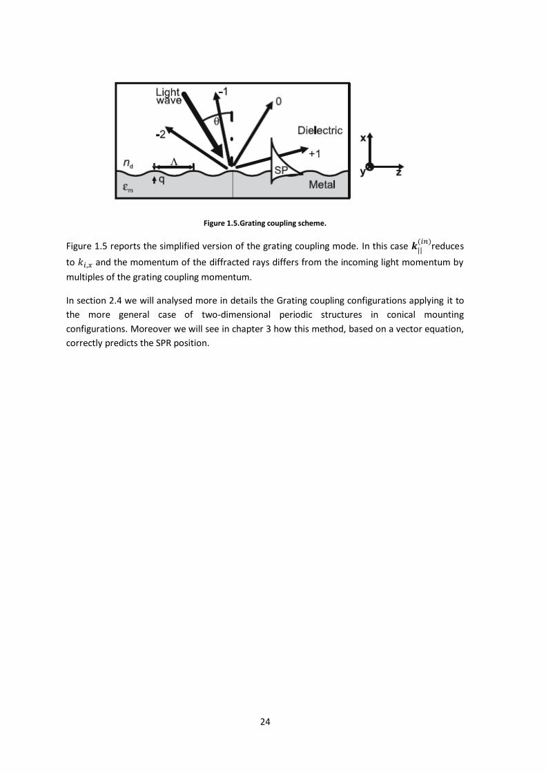
Nevertheless we are interested here in periodic nano-structures where the grating momentum
can be described by a vector 𝑮 constant in all the space. Hence the missing momentum for the
excitation of the SPP is supplied by the grating itself (See Figure 1.5), satisfying this simple vector
equation:
𝒌𝑆𝑃𝑃 = 𝒌||(𝑖𝑛)
+𝑚𝑮 (1.33)
where 𝒌𝑆𝑃𝑃 is the plasmonic momentum, 𝒌||(𝑖𝑛)
is the projection onto the grating plane of the
incoming light momentum and 𝑚 ∈ ℤ is the grating diffraction order that allow the coupling.
This equation can be simplified to a scalar form if all the three vectors are aligned:
𝑘𝑆𝑃𝑃 = 𝑘0√𝜖𝑑 sin 𝜃 +𝑚|𝑮| = 𝑘𝑥,𝑛 (1.34)
where |𝑮| =2𝜋
Λ is the modulus of the grating momentum and Λ is the grating period.
When this resonance condition is satisfied by the n-th diffraction order the diffraction the input
light power is delivered to the SPP and experimentally a minimum in the reflectance or a
maximum in the grating transmittance are observed.
24
Figure 1.5.Grating coupling scheme.
Figure 1.5 reports the simplified version of the grating coupling mode. In this case 𝒌||(𝑖𝑛)
reduces
to 𝑘𝑖,𝑥 and the momentum of the diffracted rays differs from the incoming light momentum by
multiples of the grating coupling momentum.
In section 2.4 we will analysed more in details the Grating coupling configurations applying it to
the more general case of two-dimensional periodic structures in conical mounting
configurations. Moreover we will see in chapter 3 how this method, based on a vector equation,
correctly predicts the SPR position.
25
1.3 Surface plasmon resonance sensors
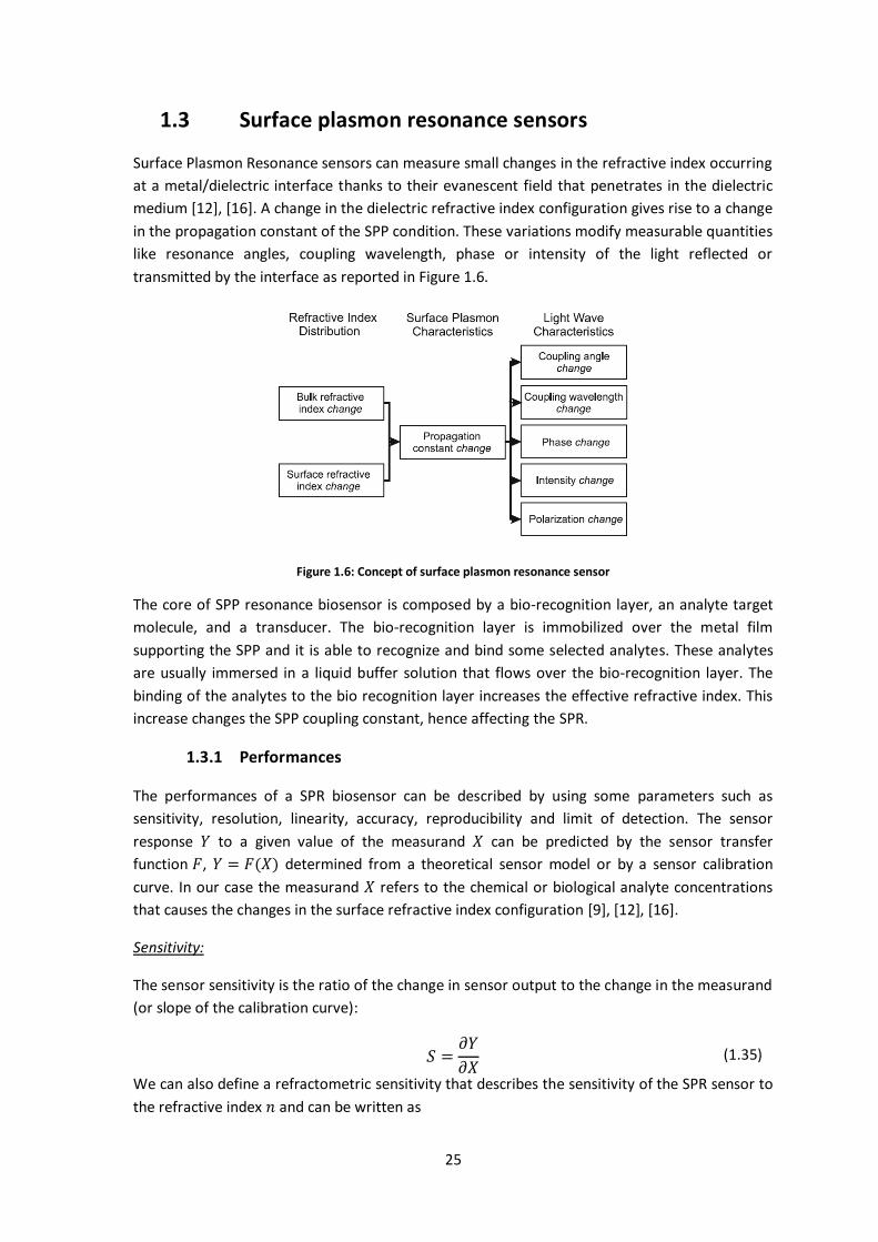
Surface Plasmon Resonance sensors can measure small changes in the refractive index occurring
at a metal/dielectric interface thanks to their evanescent field that penetrates in the dielectric
medium [12], [16]. A change in the dielectric refractive index configuration gives rise to a change
in the propagation constant of the SPP condition. These variations modify measurable quantities
like resonance angles, coupling wavelength, phase or intensity of the light reflected or
transmitted by the interface as reported in Figure 1.6.
Figure 1.6: Concept of surface plasmon resonance sensor
The core of SPP resonance biosensor is composed by a bio-recognition layer, an analyte target
molecule, and a transducer. The bio-recognition layer is immobilized over the metal film
supporting the SPP and it is able to recognize and bind some selected analytes. These analytes
are usually immersed in a liquid buffer solution that flows over the bio-recognition layer. The
binding of the analytes to the bio recognition layer increases the effective refractive index. This
increase changes the SPP coupling constant, hence affecting the SPR.
1.3.1 Performances
The performances of a SPR biosensor can be described by using some parameters such as
sensitivity, resolution, linearity, accuracy, reproducibility and limit of detection. The sensor
response 𝑌 to a given value of the measurand 𝑋 can be predicted by the sensor transfer
function 𝐹, 𝑌 = 𝐹(𝑋) determined from a theoretical sensor model or by a sensor calibration
curve. In our case the measurand 𝑋 refers to the chemical or biological analyte concentrations
that causes the changes in the surface refractive index configuration [9], [12], [16].
Sensitivity:
The sensor sensitivity is the ratio of the change in sensor output to the change in the measurand
(or slope of the calibration curve):
𝑆 =𝜕𝑌
𝜕𝑋 (1.35)
We can also define a refractometric sensitivity that describes the sensitivity of the SPR sensor to
the refractive index 𝑛 and can be written as
26
𝑆𝑅𝐼 =𝜕𝑌
𝜕𝑛 (1.36)
and similarly a sensitivity of an SPR biosensor to the concentration of analyte 𝑐
𝑆𝑐 =𝜕𝑌
𝜕𝑐 1.37
The sensitivity of a SPR biosensor to the concentration of the analyte can be decomposed into
two main factors:
𝑆𝑐 =
𝜕𝑌
𝜕𝑐=𝜕𝑌
𝜕𝑛
𝑑𝑛(𝑐)
𝑑𝑐= 𝑆𝑅𝐼𝑆𝑛𝑐 (1.38)
where 𝑆𝑛𝑐 is derived from the refractive index change caused by the binding of analyte
concentration 𝑐 to the biorecognition layer.
The sensitivity of a SPR sensor to a refractive index 𝑆𝑅𝐼 is given by two contributions:
𝑆𝑅𝐼 =𝜕𝑌
𝜕𝑛𝑒𝑓𝑓
𝛿𝑛𝑒𝑓𝑓𝛿𝑛𝑏
= 𝑆𝑅𝐼1𝑆𝑅𝐼2 (1.39)
The first term 𝑆𝑅𝐼1 depends on the method of excitation of surface plasmons and it represents
an instrumental contribution. The second term 𝑆𝑅𝐼2 describes the sensitivity of the effective
index of a surface plasmon to the refractive index and it is independent respect to the SPP
excitation method. These last term mainly depends on the profile of the refractive index (for
instance a bulk or surface refractive index changes).
Resolution:
The resolution of a SPR biosensor is defined as the smallest change in the bulk refractive index
that produces a detectable change in the sensor output and it is strictly related to the level of
uncertainty of the sensor output. The resolution 𝜎𝑅𝐼 is typically expressed in terms of the
standard deviation of the sensor output noise, 𝜎𝑠𝑜, translated to the refractive index of bulk
medium, 𝜎𝑅𝐼 = 𝜎𝑠𝑜/𝑆𝑅𝐼 .
Dominant sources of noise are the fluctuations in the light intensity emitted by the light source,
the laser in our case, the shot noise associated with photon statistics, associated to the
conversion of the light intensity into electric signal.
Noise in the intensity of light emitted by the light source is proportional to the intensity and its
standard deviation 𝜎𝐿 can be given as 𝜎𝐿 = 𝜎𝑟𝐿𝐼 where 𝜎𝑟𝐿 is relative standard deviation and 𝐼
is the measured light intensity.
Shot noise is associated to random arrival of photons on a detector and the corresponding
random production of photoelectrons. Photon flux usually obeys Poisson statistics and produces
a shot noise 𝜎𝑆 which is directly proportional to the square root of the detected light intensity:
𝜎𝑆 = 𝜎𝑟𝑆√𝐼 where 𝜎𝑟𝑆 is relative standard deviation. Detector noise consists of several
contributions that originate mostly in temperature noise and its standard deviation 𝜎𝐷 is
independent on the light intensity.
The resulting noise of a measured light intensity 𝜎𝐼 is a statistical superposition of all the noise
components and it is expressed as:

27
𝜎𝐼(𝐼) = √𝐼2𝜎𝑟𝐿2 + 𝐼𝜎𝑟𝑆
2 + 𝜎𝐷 2 (1.40)
Linearity, accuracy, and reproducibility:
Sensor linearity defines the extent to which the relationship between the measurand and the
sensor output is linear over the working range. Linearity is usually specified in terms of the
maximum deviation from a linear transfer function over the specified dynamic range. Sensors
with linear transfer function are desirable as they require fewer calibration points to produce an
accurate sensor calibration. However, response of SPR biosensors is usually a non-linear function
of the analyte concentration and therefore calibration needs to be carefully considered.
The sensor accuracy describes the agreement between a measured value and a true value of the
measurand i.e. the analyte concentration.
The sensor reproducibility refers to the ability of the sensor to return the same output when
measuring the same value of measurand.
Limit of detection (LOD)
LOD is the concentration of analyte 𝑐𝐿derived from the smallest measure 𝑌𝐿 that can be
detected with reasonable certainty. The value is given by
𝑌𝐿𝑂𝐷 = 𝑌𝑏𝑙𝑎𝑛𝑘 +𝑚 𝜎𝑏𝑙𝑎𝑛𝑘 (1.41)
where 𝑌𝑏𝑙𝑎𝑛𝑘 is the mean of the blank (sample with no analyte) measures, 𝜎𝑏𝑙𝑎𝑛𝑘 is the standard
deviation of the blank measures, and 𝑚 is a numerical factor chosen according to the confidence
level desired (typically 𝑚 = 2 or 3).
As 𝑐𝑏𝑙𝑎𝑛𝑘 = 0, the LOD concentration 𝑐𝐿𝑂𝐷 can be expressed as:
𝑐𝐿𝑂𝐷 = 𝑚 𝜎𝑏𝑙𝑎𝑛𝑘
𝑆𝑐(𝑐 = 0)⁄ (1.42)

28
1.3.2 Detection techniques
Figure 1.7 Main detection formats used in SPR biosensors: A) direct detection; B) sandwich detection format; C) competitive detection format; D) inhibition detection format.
In the previous section (eq 1.38) we have seen that the SPP sensitivity to some analyte
concentrations is governed by two factors one due to the detection method 𝑆𝑅𝐼 and the other
one due to the ability of the analyte to cause a change in the refraction index 𝑆𝑛𝑐.
If only the detection method is considered 𝑆𝑅𝐼 we can defined a resolution of the instrument by
defining the small refractive index variations that can be detected. This value seems to have
reached an intrinsic limit of 10-7 RIU [25] even if some authors claims it could be reduced until
10-8 RIU [26]–[30]. Nevertheless this seems to be an ultimate limits for this detection technique
and therefore in order to increase the resolution and the LOD for an analyte concentration
several detection formats were developed. We report the main ones in Figure 1.7 [12].
The detection format is chosen on the basis of analyte target molecules size, interaction with the
bio-recognition layer, and range of concentrations.
The simplest detection scheme is the direct one reported in Figure 1.7a. In this case the direct
binding between the analyte and the biorecognition layer is able to produce a sufficient
response of the sensor in the desired analyte concentrations range. The specificity and LOD can
be improved by using the sandwich detection format (Figure 1.7b). Here a second antibody
attaches to the bound analyte layer enhancing in this way the SPP response, proportionally to
the bounded analytes.

29
Small analytes (molecular weight < 5000) often does not generate a sufficient change in the
refractive index. This is due to the fact that the analyte molecules usually are captured by a bio
recognition layer that acts as a spacer between them and the metal surface. This spacer
decreases the molecular sensitivity 𝑆𝑛𝑐, due to the evanescent nature of the SPP electric field
inside the dielectric. Thanks to the competitive or inhibition detection format one can overcome
this low 𝑆𝑛𝑐 value.
The competitive detection format is reported in Figure 1.7c. Here the surface is coated with
fixed number of binding sites i.e. antibody. In the solution both analytes and bigger conjugate
analyte molecules are present. Since the two species compete for the same binding site, and
only if the large conjugate molecules bound we can detect a signal, the SPR variations is
inversely proportional to the analyte concentration.
The inhibition method is presented in Figure 1.7d. Here fixed concentration of antibodies is
mixed in a solution with an unknown concentration of their affinity analyte. On the surface
sensors the same analytes were previously immobilized. When the solution containing both
antibodies and analytes flows over the surface the free antibodies bind with the immobilized
analyte. Also in this case the response is inversely proportional to the analyte concentration
since the greater is the SPR signal the more antibodies are free to bind and this means a low
analyte concentration.
30
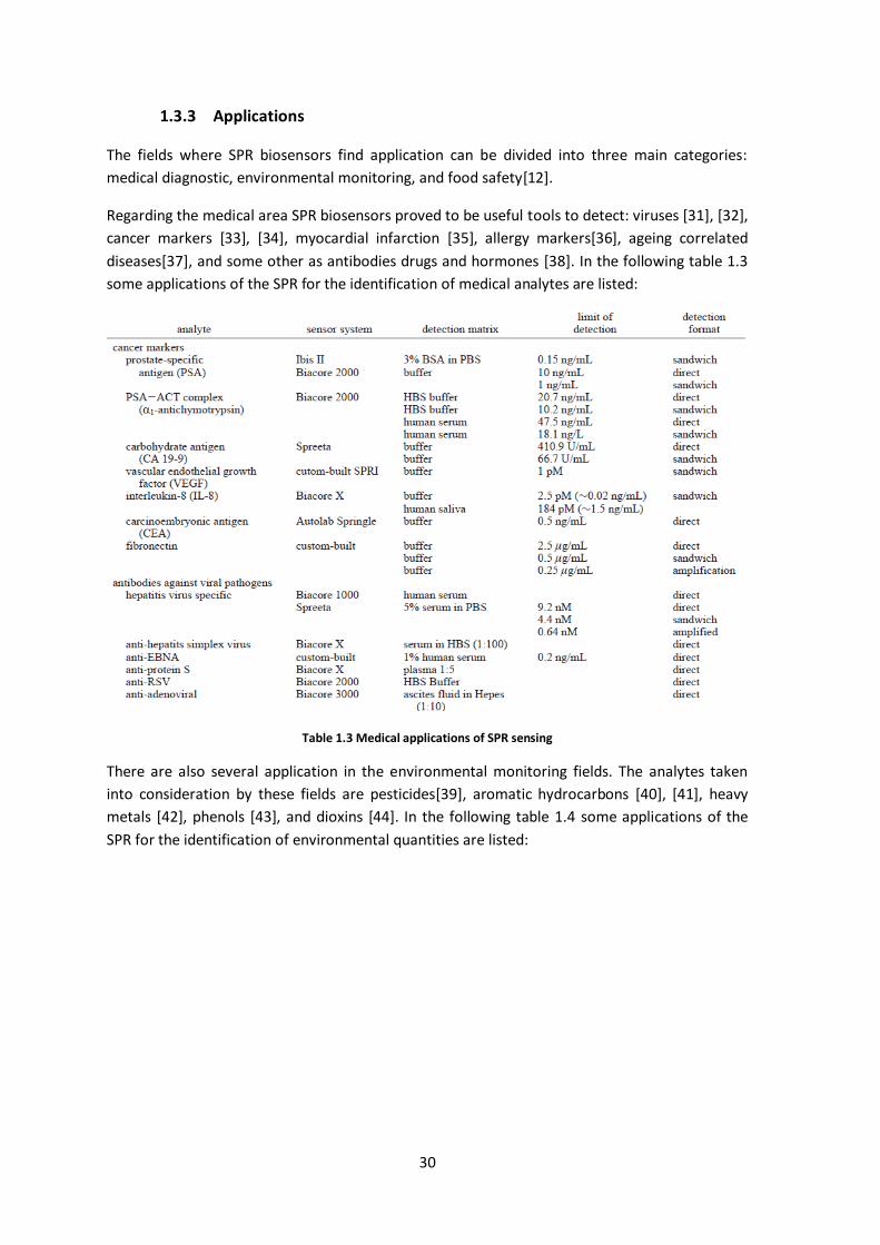
1.3.3 Applications
The fields where SPR biosensors find application can be divided into three main categories:
medical diagnostic, environmental monitoring, and food safety[12].
Regarding the medical area SPR biosensors proved to be useful tools to detect: viruses [31], [32],
cancer markers [33], [34], myocardial infarction [35], allergy markers[36], ageing correlated
diseases[37], and some other as antibodies drugs and hormones [38]. In the following table 1.3
some applications of the SPR for the identification of medical analytes are listed:
Table 1.3 Medical applications of SPR sensing
There are also several application in the environmental monitoring fields. The analytes taken
into consideration by these fields are pesticides[39], aromatic hydrocarbons [40], [41], heavy
metals [42], phenols [43], and dioxins [44]. In the following table 1.4 some applications of the
SPR for the identification of environmental quantities are listed:

31
Table 1.4 Environmental applications of SPR
SPR sensors finds applications also in food analysis. In these fields they are used to monitor
pathogens [45], toxins[46], drug residues [47], vitamins, hormones, antibodies [48], chemical
contaminants, allergens, and proteins [49]. Some applications of the SPR for the identification of
different bacteria in foods are listed in table 1.5:

32
Table 1.5 Food safety application of SPR.
Many other examples of SPR sensing applications could be listed here but this goes far beyond
our goal. In fact, since SPR detection is nowadays accepted as a standard laboratory tools used
to monitor the interaction kinetics between probe and analyte, it is almost impossible list all its
application. For a complete review of this sensing field, update to the year 2008, the reader is
reminded to the Homola work [12].

33
2 Surfaces Simulation Methods
In this chapter we will exploit different methods used for the reflectance and transmittance
simulation from a nanostructured surface. The first two methods i.e. the Rigorous Coupled Wave
Analysis Method (RCWA) [50]–[54]and the Chandezon Method (CM) [55]–[57], are currently
widely used by the scientific community to analyse both unidimensional and bidimensional
periodical structures[58]–[62]. Even if the first description of these two methods dates back to
the 1980, they are constantly studied for improving their efficiency and applications.
The Finite Element Method (FEM) is nowadays one of the most widespread numerical
techniques for the simulation of structures with applications that reach electromagnetic [63],
thermal, chemical and mechanical fields. Since its implementation is very complex, dedicated
software were developed over the years. In our case we used the radio frequency package
implemented in Comsol v3.5 in order to solve both unidimensional and bidimensional periodic
structures.
Finally we will generalize the vector model introduced in section 1.2.2. This method is the easiest
way to predict where Surface Plasmon Resonance will occur when periodic structured surface is
used. Nevertheless it does not give any information about their shape in relation with the
periodic geometrical structure.
Our developed simulation methods will reproduce the behaviour of periodic structures lighted in
conical mounting configuration. The general scheme is reported in Figure 2.1.
Figure 2.1 Conical mounting configuration scheme.
Figure 2.1 represents a unidimensional grating (yellow lines) lighted in conical configuration. The
grating surface lays in the 𝑥, 𝑦 plane. The incident wave vector 𝜂𝑑𝑘0⃗⃗⃗⃗ along with the vector
normal to the grating plane defines the scattering plane (cyan transparent layer). The incoming
light electric field �⃗� lays on the polarization ellipse (red coloured ellipse).
Three main angles described this configuration: the incident angle 𝜃; the polarization angle 𝜓,
and the azimuthal angle 𝜙. As we can see 𝜙 is defined as the angle between the grating
momentum 𝐺 (In figure2.1 it coincides with the 𝑥- axis) and the scattering plane. When 𝜓 = 0°
we will refer to the transverse magnetic polarization mode (TM) meanwhile when 𝜓 = 90° we
will refer to the Transverse Electric polarization mode (TE).

34
Looking at this reference system the incoming light wave vector can be written as:
𝜂𝑑𝑘0⃗⃗⃗⃗ = 𝜂𝑑 {
𝑘0𝑠𝑖𝑛𝜃𝑐𝑜𝑠𝜙𝑘0𝑠𝑖𝑛𝜃𝑠𝑖𝑛𝜙−𝑘0𝑐𝑜𝑠𝜃
(2.1)
And the electric field as:
�⃗� = 𝐸0 {
𝑐𝑜𝑠𝜓 𝑐𝑜𝑠𝜃 𝑐𝑜𝑠𝜙 + 𝑠𝑖𝑛𝜓 𝑠𝑖𝑛𝜙𝑐𝑜𝑠𝜓 𝑐𝑜𝑠𝜃 𝑠𝑖𝑛𝜙 − 𝑠𝑖𝑛𝜓 𝑐𝑜𝑠𝜙
𝑐𝑜𝑠𝜓 𝑠𝑖𝑛𝜃 (2.2)
The unidimensional periodic grating structures can be simulated in the conical mounting
configuration by using the RCWA and the FEM methods we developed, meanwhile we restricted
the CM to light incoming with 𝜙=0° and in TM or TE polarization mode. The simulation of the
two dimensional periodic structures in conical mounting configuration will be performed by
using only the FEM method.
2.1 Rigorous Coupled Wave Analysis Method
The RCWA method or Fourier Modal Method (FMM) was developed over the ‘80s and ‘90s. Its
aim is to rigorously solve the electromagnetic fields problem inside a periodic structure, and
therefore calculate the light diffraction coefficients. One of the first paper on the subject dates
back to 1981 [50] but the true success of this method arrived in 1995 were the work of M.G.
Moharam [51], [52]and P. Lalanne[64] improved the convergence of this method.
Here we will briefly describe this method and the modifications that must be introduced to
improve the method convergence and stability. Here we will strictly follow the formulation
proposed in [52], where only the TM lighting mode for φ = 0° is considered. Nevertheless we
implemented a full model to perform the simulation in conical mounting configuration.
Figure 2.2 Geometry for the study of diffraction grating using the RCWA method
Figure 2.2 shows how a general grating profile is treated by the RCWA method. There is an
upper continuum medium where an incident plane wave along with the grating reflected rays

35
propagate. The incident light incomes with an angle 𝜃 respect to the normal of the grating plane.
The transmitted rays propagate in a lower medium that also acts as the grating substrate.
The region between the upper and lower medium is the grating region and it is characterized by
a periodic distribution of the dielectric constant along the x-direction. Is therefore possible to
develop it in a Fourier series:
휀(𝑥, 𝑧) = ∑휀ℎ(𝑧)
ℎ
exp (𝑗2𝜋ℎ
Λ 𝑥) (2.3)
Here 휀ℎ(𝑧) is the ℎ-th Fourier component which incorporates the z-dependence of the dielectric
function. In order to apply the RCWA method we need to eliminate the z-dependency of the
Fourier component. We can achieve this by dividing the grating region in an arbitrary number of
slabs having a definite height as shown in figure 2.2. It is obvious that increasing the number of
layers every grating profile can be describe with the desired accuracy; and it is also evident that
this method well describe the case of a digital grating. In this way the dielectric constant inside
the grating region acquires this mathematical formulation:
휀𝑙(𝑥) = ∑휀𝑙,ℎℎ
exp (𝑗2𝜋ℎ
Λ 𝑥) ; 𝐷𝑙 − 𝑑𝑙 < 𝑧 < 𝐷𝑙 ; 𝐷𝑙 =∑𝑑𝑙
𝑙
𝑝=1
(2.4)
where 𝑑𝑙 represent the thickness of the 𝑙-th layer. The field in the upper region of the grating is
represented by:
𝐻𝐼,𝑦 = 𝑒𝑥𝑝{−𝑗𝑘0𝜂𝐼[sin(𝜃) 𝑥 + cos(𝜃) 𝑧]} +∑𝑅𝑖𝑒𝑥𝑝{−𝑗[𝑘𝑥𝑖𝑥 − 𝑘𝐼,𝑧𝑖𝑧]}
𝑖
(2.5)
where the first term represents the incident field meanwhile the second term represents the
reflected component of the field.
In the lower medium we got the transmitted rays:
𝐻𝐼𝐼,𝑦 =∑𝑇𝑖𝑒𝑥𝑝{−𝑗[𝑘𝑥𝑖𝑥 − 𝑘𝐼𝐼,𝑧𝑖(𝐷𝐿 − 𝑧)]}
𝑖
(2.6)
In all the fields expression we hide the temporal dependency 𝑒𝑖𝜔𝑡. The quantity 𝑘𝑥𝑖, 𝑘𝐼𝐼,𝑧𝑖 , and
𝑘𝐼,𝑧𝑖 are determined from the Rayleigh-Floquet field expansion:
𝑘𝑥𝑖 = 𝑘0[𝜂𝐼 sin(𝜃) − 𝑖 (𝜆0 Λ)⁄ ]
𝑘𝑙,𝑧𝑖 = √𝑘02𝜂𝑙
2 − 𝑘𝑥𝑖2 ; 𝑙 = 𝐼, 𝐼𝐼
(2.7)
The tangential magnetic and electric field in the 𝑙-th grating layer are expressed through a
Fourier expansion:
𝐻𝑙,𝑔𝑦 =∑𝑈𝑙,𝑦𝑖𝑖
(𝑧) exp(−𝑗𝑘𝑥𝑖𝑥)
𝐸𝑙,𝑔𝑥 = 𝑗√𝜇0휀0∑𝑆𝑙,𝑥𝑖𝑖
(𝑧)exp (−𝑗𝑘𝑥𝑖𝑥)
(2.8)
By using the Maxwell’s equations:
∇ × 𝐻 = 휀0휀𝜕𝐸
𝜕𝑡 ; ∇ × 𝐸 = −
𝜇0𝜇𝜕𝐻
𝜕𝑡 (2.9)

36
The three following useful equations can be obtained:
𝜕𝐻𝑦𝜕𝑧
= −𝑗𝜔휀0휀(𝑥, 𝑧)𝐸𝑥
𝜕𝐻𝑦𝜕𝑥
= 𝑗𝜔휀0휀(𝑥, 𝑧)𝐸𝑧
𝜕𝐸𝑥𝜕𝑧
= −𝑗𝜔𝜇0𝜇𝐻𝑦 + 𝜕𝐸𝑧𝜕𝑥
(2.10)
By solving the equations 2.10 inside each grating slab, and taking into account that in our case
𝜇 = 1 we get the following relation:
𝜕2𝐻𝑙,𝑔𝑦𝜕𝑧2
= [−𝑘02 휀(𝑥) + 휀(𝑥)
𝜕
𝜕𝑥
1
휀(𝑥)
𝜕
𝜕𝑥]𝐻𝑙,𝑔𝑦 (2.11)
Since the grating is periodic, we assume that the fields 𝐻𝑙,𝑔𝑦, and the dielectric constant inside
each slab can be written as a Fourier sum. Hence the equation 2.11 can be solved considering
the functions exp (−𝑗𝑘𝑥𝑖𝑥) as a base. Therefore it assumes the sequent matrix form:
𝜕2𝐔𝑙,𝑦𝜕(𝑧′)2
= [𝐄𝑙][𝐊𝑥𝐄𝑙−1𝐊𝑥 − 𝐈]𝐔𝑙,𝑦 (2.12)
where 𝑧′ = 𝑘0𝑧, 𝐈 is the unitary matrix, 𝐊𝑥 is a diagonal matrix with diagonal element 𝑘𝑥𝑖 𝑘0⁄ ,
and 𝐄𝑙 is the matrix with its 𝑖, 𝑝-th element 휀𝑙,𝑖−𝑝.
Being the functions 𝑈𝑙,𝑦𝑖(𝑧) only a function of 𝑧, they can be solved assuming a finite number 𝑛
for the Rayleigh expansion of the fields, since the matrix equation 2.12 represents a standard
eigenvalue problem. Therefore the analytical expression for 𝑈𝑙,𝑦𝑖(𝑧) becomes:
𝑈𝑙,𝑦𝑖(𝑧) = ∑ 𝑤𝑙,𝑖,𝑚
𝑛
𝑚=1
{𝑐𝑙,𝑚+ exp[−𝑘0𝑞𝑙,𝑚(𝑧 − 𝐷𝑙 + 𝑑𝑙)]
+ 𝑐𝑙,𝑚− exp[𝑘0𝑞𝑙,𝑚(𝑧 − 𝐷𝑙)]}
(2.13)
where 𝑤𝑙,𝑖,𝑚 are the elements of the eigenvector matrix 𝐖𝑙 and 𝑞𝑙,𝑚 are the square root with
positive real part of the eigenvalues of the matrix [𝐄𝑙][𝐊𝑥𝐄𝑙−1𝐊𝑥 − 𝐈]. The coefficients 𝑐𝑙,𝑚
+ and
𝑐𝑙,𝑚− are unknown constant that will be determined by imposing the adequate boundary
conditions between each grating layer.
In order to fully solve the system we need also to find the condition for the tangential
component of the electric field 𝐸𝑥 which are expressed in a matrix form by the equation:
𝐒𝑙,𝑥 = [𝐄𝑙]𝜕𝐔𝑙,𝑦𝜕(𝑧′)
(2.14)
Imposing the boundary conditions between the input region and the first grating layer (𝑧=0) we
obtain:
[𝛿𝑖0
𝑗𝛿𝑖0𝑐𝑜𝑠(𝜃)/𝜂𝐼] + [
𝐈−𝑗𝐙𝐼
]𝐑 = [𝐖1 𝐖1𝐗1𝐕1 −𝐕1𝐗1
] [𝐜1+
𝐜1−] (2.15)
By applying it at the boundary between the 𝑙 − 1 and 𝑙 grating layers we have:
[𝐖𝑙−1𝐗𝑙−1 𝐖𝑙−1
𝐕𝑙−1𝐗𝑙−1 −𝐕𝑙−1] [𝐜𝑙−1+
𝐜𝑙−1− ] = [
𝐖𝑙 𝐖𝑙𝐗𝑙𝐕𝑙 −𝐕𝑙𝐗𝑙
] [𝐜𝑙+
𝐜𝑙−] (2.16)
At the boundary between the last grating layer and the substrate region (𝑧 = 𝐷𝐿) we get:

37
[𝐖𝐿𝐗𝐿 𝐖𝐿
𝐕𝐿𝐗𝐿 −𝐕𝐿] [𝐜𝐿+
𝐜𝐿−] = [
𝐈𝑗𝐙𝐼𝐼
]𝐓 (2.17)
In this cases 𝐕𝑙 = 𝐄𝑙−1𝐖𝑙𝐐𝑙 with 𝐐𝑙 a diagonal matrix with the diagonal elements 𝑞𝑙,𝑚, 𝐗𝐿 is a
diagonal matrix with the diagonal elements exp(−𝑞𝑙,𝑚𝑑𝑙); 𝐙𝐼 and 𝐙𝐼𝐼 are diagonal matrix with
the element 𝑘𝐼,𝑧𝑖 𝜂𝐼2⁄ 𝑘0 and 𝑘𝐼𝐼,𝑧𝑖 𝜂𝐼𝐼
2⁄ 𝑘0 respectively. 𝐑 and 𝐓 are column matrixes with the
reflection and transmission coefficient respectively meanwhile 𝛿𝑖0 is the usual Kronecker
function. All these boundary condition can be summarized in an easy formulation:
[𝛿𝑖0
𝑗𝛿𝑖0𝑐𝑜𝑠(𝜃)/𝜂𝐼] + [
𝐈−𝑗𝐙𝐼
]𝐑 = ∏[𝐖𝑙 𝐖𝑙𝐗𝑙𝐕𝑙 −𝐕𝑙𝐗𝑙
] [𝐖𝑙𝐗𝑙 𝐖𝑙
𝐕𝑙𝐗𝑙 −𝐕𝑙]−1
[𝐈𝑗𝐙𝐼𝐼
]𝐓
𝐿
𝑙=1
(2.18)
This expression may appear simple but it cannot be solved straightforwardly due to the
numerical error that will be produce in the matrix inversion. This errors are due to the very small
number produced by exp(−𝑞𝑙,𝑚𝑑𝑙) in the diagonal element of the matrix 𝐗𝑙. In order to avoid
these numerical errors we implemented in our code the full solution approach described in [52].
Once the coefficients 𝐑 and 𝐓 are found the reflectance and transmittance of the diffracted ray
can be found by using these two equations:
𝐷𝐸𝑟𝑖 = 𝑅𝑖𝑅𝑖
∗Re[𝑘𝐼,𝑧𝑖 𝑘0𝜂𝐼 cos(𝜃)⁄ ]
𝑇𝐸𝑟𝑖 = 𝑇𝑖𝑇𝑖∗Re[𝑘𝐼𝐼,𝑧𝑖 𝜂𝐼 𝑘0𝜂𝐼𝐼
2 cos (𝜃)⁄ ] (2.19)
The accuracy of the solution returned by this method depends on the number of the retained
harmonics in the field expansion. Nevertheless the convergence rate of the diffraction efficiency
parameters as a function of the number of retained harmonics depends on the light polarization
i.e. it is slower for the TM mode respect to the TE one. A straight forward solution of this
problems comes from the work of Lalanne [64] that propose to substitute the matrix equation
2.12 with this one:
𝜕2U𝑙,𝑦𝜕(𝑧′)2
= [A𝑙−1][K𝑥E𝑙
−1K𝑥 − I]U𝑙,𝑦 (2.20)
Being 𝐴 the matrix formed by the inverse permittivity harmonic coefficient. He also further
developed this technique and give the complete reformulation for the conical mounting
problem.
Our standard grating description is performed by the model reported in figure 2.3 which shows
the grating periodic cell cross section.

38
Figure 2.3 Standard grating geometrical description.
As we can see from Figure 2.3 our grating is a five layers system. The polycarbonate substrate is
described by the blue area, the grey area represents the silver layer and the green layer that
covers all the upper interface describes the functionalization layer. The dashed lines represent
the interface between each of the grating layer where boundary conditions must be imposed. In
most of the grating slabs the dielectric constant is described by a rectangular function. For
example, if we consider the fifth layer, that corresponds to the silver-polycarbonate-silver layer,
its Fourier transform coefficients are:
휀5,𝑚 = 휀𝑝𝑜𝑙𝑦𝑠𝑖𝑛𝑐(𝑚) + (휀𝑝𝑜𝑙𝑦 − 휀𝐴𝑔)𝑓𝑑𝑜𝑤𝑛(𝑠𝑖𝑛𝑐(𝑚𝑓𝑑𝑜𝑤𝑛)) (2.21)
The layer that needs a particular description is the second one (from the upper interface of the
grating), where we have three different materials that describe the dielectric constant. In this
case the Fourier coefficients becomes:
휀2,𝑚 = 휀𝑎𝑖𝑟𝑠𝑖𝑛𝑐(𝑚) + (휀𝑓𝑢𝑛𝑐 − 휀𝑎𝑖𝑟)𝑓𝑓𝑢𝑛𝑐 (𝑠𝑖𝑛𝑐(𝑚𝑓𝑓𝑢𝑛𝑐))
+ (휀𝐴𝑔 − 휀𝑓𝑢𝑛𝑐)𝑓𝑢𝑝(𝑠𝑖𝑛𝑐(𝑚𝑓𝑢𝑝)) (2.22)
In order to test the implemented method we consider in figure 2.4 the diffraction coefficients
obtained by using the Moharam and Lalanne implementations. We performed the calculations
for both the TM and TE polarization, considering an incident angle of 15° and an azimuthal angle
of 0°. In reference to figure 2.3 the geometrical parameters used in this simulation are
respectively:
λ Λ fup fdown hdown hup hslab hfunc 휀𝑎𝑖𝑟 휀𝐴𝑔 휀𝑓𝑢𝑛𝑐 휀𝑝𝑜𝑙𝑦
635 nm
740 nm
0.45 0.3 20 nm
20 nm
35 nm
1.5 nm
1 -17-0.7i
1 2.4964
Table 2.1 Parameters used for the digital grating cross section description

39
Figure 2.4 A comparison between the diffraction efficiency convergence by using the old and new method for: (a)
TM, and (b) TE polarization
In figure 2.4 we reported the Diffraction efficiency of the R-1 reflected ray as a function of the
number of retained Rayleigh orders in the field expansion (2N+1). The continuous red line refers
to the Moharam formulation meanwhile the blue circles refers to the Lalanne formulation. As
we can see the method quickly converge in both the formulation for the TE polarization (Figure
2.4b), while for the TM (Figure 2.4a) we get an enormous improvement of the convergence rate
by adding the Lalanne modifications. Also the oscillatory behaviour is completely suppressed.
A complete explanation of the numerical problem of the different rate convergence can be
found in the work of L. Li [65] and further developed for the two dimensional periodic structures
case by Schuster [54]. The treatment of this topics goes far beyond our purpose here;
nevertheless we can see from figure 2.4 that our implemented code well converge if a number N
= 100, that corresponds to 2N+1 retained harmonics, is used.
2.2 Chandezon method
The first Implementation of the Chandezon or curvilinear, or differential method dates back to
1982 [55]. The difference between CM and RCWA it is well explained by figure2.5 [66].
Figure 2.5 Difference in the grating profile treatment between the RCWA and Chandezon Method.
Starting from the grating profile describe in the central panel of figure 2.5, the RCWA method
divides the grating region in a huge amount of layers each one with a particular step dielectric
function profile 휀(𝑥) (left panel of figure 2.5), while the Chandezon method, through a change in
the coordinates system, transforms the grating profile in a planar interface, eliminating in this
way the 𝑧-dependency of the dielectric function inside the grating region. In the new coordinate
0 50 100 1500.016
0.018
0.02
0.022
0.024
0.026
0.028
0.03
0.032
0.034
number of retained order
Difrr
actio
n e
ffic
en
t o
f R
1
TM polarization
Moharam
Lalanne
0 50 100 1500.01190
0.011925
0.01195
0.011975
0.01200
number of retained order
TE polarization
Moharam
Lalanne
b)a)

40
system the problem is reduced to the calculations of transmission and reflection of light passing
through a set of planar interfaces.
For briefly illustrate the method we will follow the derivation showed by Li [67]. Nevertheless we
generalized the Li method description allowing a multilayer coating for the grating, hence we
can describe the thin silver film, and the functionalization coating layer. The method we
implemented reproduces the behaviour of the grating lighted by the TM polarization mode, and
with the grating slits perpendicular to the scattering plane, i.e. 𝜙= 0°. It is also suited for the
description of discontinuous grating profile such as a trapezoidal or triangular one because it
uses the same electromagnetic formulation introduced in [58], [68].
Figure 2.6 schematic for the CM implementation.
We considered a periodically corrugate interface, invariant in the 𝑧-direction between two
homogeneous isotropic media with refractive index 𝜂𝐼 , 𝜂𝐼𝐼 respectively. The grating period and
amplitude are denoted by 𝛬 and 𝑑. The incident angle is 𝜃 and the scattering plane is
perpendicular to the grating slits. The harmonic time convention exp (−𝑖𝜔𝑡) is assumed. In
figure 2.6 the grating is described by a function 𝑦 = 𝑎(𝑥) that splits the space into two regions
called 𝐷+ , 𝐷−.
The space could be also further divided into three regions by using the dashed lines: 𝐷1, 𝐷2, 𝐷0.
In the domains 𝐷1,and 𝐷2 the field can be written as in eq. 2.5 and 2.6 by using the Ryleigh -
Floquet expansion:
𝐹 = ∑𝐴𝑚(𝑝)±
𝑚
exp(𝑗𝛼𝑚𝑥 ± 𝑖𝛽𝑚(𝑝)𝑦 ) , 𝑝 = 1,2 (2.23)
where 𝐹 = 𝐻𝑧, 𝛼𝑚 = 𝜂1𝑘0 sin(𝜃) + 𝑚𝐾, 𝐾 = 2𝜋 Λ⁄ , 𝛽𝑚(𝑝)
= (𝜂𝑝2𝑘0
2 −𝛼𝑚2 )
1 2⁄ with
Re [𝛽𝑚(𝑝)] + Im[ 𝛽𝑚
(𝑝)] > 0, and 𝐴𝑚
(𝑝)± are constant amplitudes. Since no reflected wave could
propagate in the 𝐷1 domain backward the y-direction, except for the incoming light ray, and no
transmitted wave could propagate in the substrate along the y direction we can simplify the
notation saying that 𝐴01− = 1; 𝐴𝑚
(1)+= 𝐴𝑚
(1); 𝐴𝑚
(2)−= 𝐴𝑚
(2).
This grating problem is therefore reduced to solve the Helmholtz equation in 𝐷+ and 𝐷−,
conditioned by the previously described boundary conditions at infinity, and along the grating
profile.
[𝜕2
𝜕𝑥2+𝜕2
𝜕𝑦2+ 𝑘0
2𝜇휀(𝑥, 𝑦)] 𝐹 = 0 (2.24)
41
If we consider the above equation 2.24 in the domains 𝐷+ or 𝐷− for the change of variable:
{𝑣 = 𝑥
𝑢 = 𝑦 − 𝑎(𝑥) (2.25)
The differential operators become:
{
𝜕
𝜕𝑥=𝜕
𝜕𝑣− �̇�
𝜕
𝜕𝑢𝜕
𝜕𝑦=
𝜕
𝜕𝑢
(2.26)
where �̇� = d𝑎 d𝑥⁄ . Substituting these expressions into the Helmholtz equation 2.24 we obtain
this differential operator:
𝐿(𝜕𝑢, 𝜕𝑣 , 𝑥) = 𝜕2
𝜕𝑣2− 2�̇�
𝜕
𝜕𝑣
𝜕
𝜕𝑢− �̈�
𝜕
𝜕𝑢+ (1 + �̇�2)
𝜕2
𝜕𝑢2+ 𝑘0
2𝜇휀𝑝 (2.27)
For convenience we will use 𝑥 insteadof 𝑣 to label the spatial variable since 𝑥 = 𝑣. In this
coordinate system if 𝑥 varies and 𝑢 is kept constant, the point (𝑥, 𝑢) traces curves parallel to the
grating profile, therefore 휀 remains constant.
The second order equation 2.27 can be rewritten as a pair of first order equations:
[𝑘02𝜇휀𝑝 +
𝜕2
𝜕𝑣20
0 1
](𝐹𝐹′) = [𝑖 (
𝜕
𝜕𝑣�̇� + �̇�
𝜕
𝜕𝑣) 1 + �̇�2
1 0
]𝜕
𝑖𝜕𝑢(𝐹𝐹′) (2.28)
Taking into account that the fields 𝐹 must respect the same periodicity of the grating and since
the wave in 𝐷+ and 𝐷− can be treated as plane waves we can write the differential operator:
𝜕
𝜕𝑣→ 𝑖𝜶,
𝜕
𝜕𝑢 → 𝑖𝜌 (2.29)
where 𝜶 is a diagonal matrix formed by 𝛼𝑚. By inserting this consideration into the equation 2.28 we obtain an eigenvalue problem:
[−
1
𝜷(𝑝)2 (𝜶�̇� + �̇�𝜶)
1
𝜷(𝑝)2 (1 + �̇��̇�)
𝟏 𝟎
] (𝑭𝑭′) =
1
𝜌(𝑭𝑭′) (2.30)
where 𝜷(𝑝) is a diagonal matrix formed by 𝛽𝑚(𝑝)
and �̇� is the matrix formed by the Fourier
coefficients of �̇�:
(�̇�)𝑚𝑛 = (�̇�)𝑚−𝑛 = 1
Λ∫ �̇�(𝑥)𝑒𝑥𝑝[−𝑖(𝑚 − 𝑛)𝐾𝑥]Λ
0
𝑑𝑥 (2.31)
If each block of the previous 2 × 2 matrix (eq.2.30) is truncated to 𝑁 × 𝑁, the 2𝑁 eigenvalues
obtained could be divided into two sets. The first set Σ+ contains the positive real eigenvalues
and the eigenvalues that have a positive imaginary part. The second set Σ− contains the negative
real eigenvalues and the eigenvalues that have a negative imaginary part. In the domain 𝐷+ all
the eigensolutions in Σ− except the one corresponding to the incident plane wave should be
discarded. Conversely in domain 𝐷− all the eigensolutions in Σ+ must not be considered since
we want our problem to be confined at 𝑢 = ∞.
Now we can write the z-component of the magnetic field in the domains 𝐷+ and 𝐷−.

42
𝐹+ = exp [𝑖𝛼0𝑥 − 𝑖𝛽0(1)𝑦]+ ∑ exp [𝑖𝛼𝑛𝑥 + 𝑖𝛽𝑛
(1)𝑦]
𝑛∈𝑈+
𝐴𝑛(1)
+∑exp(𝑖𝛼𝑚𝑥)
𝑚
∑ 𝐹𝑚𝑞+
𝑞∈𝑉+
exp(𝑖𝜌𝑞+𝑢)𝐶𝑞
+
𝐹− = ∑ exp [𝑖𝛼𝑘𝑥 − 𝑖𝛽𝑘(2)𝑦]
𝑘∈𝑈−
𝐴𝑘(2)
+∑exp(𝑖𝛼𝑚𝑥)
𝑚
∑ 𝐹𝑚𝑟−
𝑟∈𝑉−
exp(𝑖𝜌𝑟−𝑢)𝐶𝑟
−
(2.32)
where 𝐴𝑛(𝑝)
and 𝐶𝑞± are the unknown diffraction amplitudes, 𝐹𝑚𝑞
± are the elements of the 𝐹 part
of the 𝑞-th eigenvector and 𝑈± and 𝑉± denote the sets of the indices for the propagating and
evanescent orders in domains 𝐷± respectively.
As we can note the expression for the total field is written in a mixed variables system. It is
therefore convenient to write everything as a function of 𝑥 and 𝑢 since 𝑦 = 𝑢 − 𝑎(𝑥). This
substitution allows to expand the exponential function of 𝑎(𝑥) in a Fourier series and then to
regroup the Fourier coefficients. In this way we obtain:
𝐹+ = ∑exp(𝑖𝛼𝑚𝑥)
𝑚
{𝐿𝑚 (−𝛽0(1)) exp [−𝑖𝛽0
(1)𝑢]
+ ∑ 𝐿𝑚−𝑛 (𝛽𝑛(1))exp [𝑖𝛽𝑛
(1)𝑢]
𝑛∈𝑈+
𝐴𝑛(1)
+ ∑ 𝐹𝑚𝑞+
𝑞∈𝑉+
exp(𝑖𝜌𝑞+𝑢)𝐶𝑞
+}
𝐹− = ∑exp(𝑖𝛼𝑚𝑥)
𝑚
{+ ∑ 𝐿𝑚−𝑘 (−𝛽𝑘(2)) exp [−𝑖𝛽𝑘
(2)𝑢]
𝑘∈𝑈−
𝐴𝑘(2)
+ ∑ 𝐹𝑚𝑟−
𝑟∈𝑉+
exp(𝑖𝜌𝑟−𝑢) 𝐶𝑟
−}
(2.33)
where 𝐿𝑚(𝛾) is:
𝐿𝑚(𝛾) = 1
Λ∫ exp [𝑖𝛾𝑎(𝑥) − 𝑖𝑚𝐾𝑥]Λ
0
𝑑𝑥 (2.34)
Matching the boundary conditions at 𝑢 = 0 is equivalent to satisfy the following matrix equation:
[𝐹𝑚𝑛𝑅+ 𝐹𝑚𝑞
+ −𝐹𝑚𝑘𝑅− −𝐹𝑚𝑟
− ]
[ 𝐴𝑛(1)
𝐶𝑞+
𝐴𝑘(2)
𝐶𝑟− ]
= [−𝐹𝑚0𝑅,𝑖𝑛
] (2.35)
where 𝐹𝑚𝑛𝑅+ = 𝐿𝑚−𝑛 (𝛽𝑛
(1)), 𝐹𝑚𝑘
𝑅− = 𝐿𝑚−𝑘 (−𝛽𝑘(2)), and 𝐹𝑚0
𝑅𝑖𝑛 = 𝐿𝑚 (−𝛽0(1))
The superscript R is associated to the terms of the Rayleigh solution. The equation 2.35 still
cannot be solved since it contains N equations and 2N unknowns. The other N equations are
provided by the boundary condition of the electric field that lies in the 𝑥, 𝑦 plane. The electric
field component tangential to the grating profile is described by the function 𝐺 = 𝐸𝑥 + �̇�𝐸𝑦 . By
expressing 𝐸𝑥 and 𝐸𝑦 in terms of 𝐻𝑧 we get the following expression for 𝐺:

43
𝐺 = 𝑍0𝑖𝑘0휀
[�̇�𝜕𝐹
𝜕𝑣− (1 + �̇�2)
𝜕𝐹
𝜕𝑢] (2.36)
By using this fields expression we obtain the complete system:
[𝐹𝑚𝑛𝑅+ 𝐹𝑚𝑞
+ −𝐹𝑚𝑘𝑅− −𝐹𝑚𝑟
−
𝐺𝑚𝑛𝑅+ 𝐺𝑚𝑞
+ −𝐺𝑚𝑘𝑅− −𝐺𝑚𝑟
−]
[ 𝐴𝑛(1)
𝐶𝑞+
𝐴𝑘(2)
𝐶𝑟− ]
= [−𝐹𝑚0
𝑅,𝑖𝑛
−𝐺𝑚0𝑅,𝑖𝑛
] (2.37)
where the matrix elements are defined as follow:
𝐺𝑚𝑛𝑅+ =
𝑍0𝑘0휀1
∑[�̇�𝑚−𝑠𝛼𝑠 − (𝟏 + �̇��̇�)𝑚𝑠𝛽𝑛(1)]
𝑠
𝐿𝑠−𝑛 (𝛽𝑛(1))
𝐺𝑚𝑘𝑅− =
𝑍0𝑘0휀2
∑[�̇�𝑚−𝑠𝛼𝑠 + (𝟏 + �̇��̇�)𝑚𝑠𝛽𝑘(2)]
𝑠
𝐿𝑠−𝑘 (−𝛽𝑘(2))
𝐺𝑚0𝑅𝑖𝑛 =
𝑍0𝑘0휀1
∑[�̇�𝑚−𝑠𝛼𝑠 + (𝟏 + �̇��̇�)𝑚𝑠𝛽0(1)]
𝑠
𝐿𝑠 (−𝛽0(1))
𝐺𝑚𝑞+ =
𝑍0𝑘0휀1
∑[�̇�𝑚−𝑠𝛼𝑠 − (𝟏 + �̇��̇�)𝑚𝑠𝜌𝑞+]
𝑠
𝐹𝑠𝑞+
𝐺𝑚𝑟− =
𝑍0𝑘0휀2
∑[�̇�𝑚−𝑠𝛼𝑠 + (𝟏 + �̇��̇�)𝑚𝑠𝜌𝑟−]
𝑠
𝐹𝑠𝑟−
(2.38)
Once the system in eq. 2.37 is solved, the field coefficients 𝐴𝑛(1)
and 𝐴𝑘(2)
can be used for the
calculus of the diffraction amplitudes by using:
𝐷𝐸𝑟𝑖 =𝛽𝑛(1)
𝛽𝑛(0)|𝐴𝑛(1)|2
𝑇𝐸𝑟𝑖 = 휀1𝛽𝑘
(2)
휀2𝛽𝑛(0)|𝐴𝑘(2)|2
(2.39)
Now we will consider the generalization of the above method to a multicoated layer.
Figure 2.7 Schematic of the Chandezon method applied to the multicoated layer case
Figure 2.7 shows a four media system with three interfaces. The four media are the
polycarbonate substrate, the silver layer, the functionalization layer, and the upper medium.
The formulation for the eigenvalues problem in the upper media and in the substrate media
follows the previous description, and also in this case only the eigenvalue that respect the
bounding conditions at ∞ must be retained in the calculations. Nevertheless, in this case, the

44
matching of the tangential fields for the silver/polycarbonate interface needs to be evaluate for
𝑢 = −𝑑2, therefore 𝐹𝑚𝑘𝑅− becomes: 𝐹𝑚𝑘
𝑅−(−𝑑2) = 𝐹𝑚𝑘𝑅−exp (𝑖𝑑2𝛽𝑘
(2)) and 𝐹𝑚𝑟
− (−𝑑2) =
𝐹𝑚𝑟− exp (−𝑖𝑑2𝜌𝑟
−). The same considerations applies to the 𝐺− factor.
Inside the silver and functionalization layers all the eigenvalues and eigenvectors returned by the
equation 2.30 must be retained in the calculations, since they represents reflected and
transmitted waves inside the layer. We will call 𝐹𝑚𝜏,1± , 𝜌𝜏,1
± and 𝐹𝑚𝜏,2± , 𝜌𝜏,2
± the eigenvectors and
eigenvalues and we found inside the functionalization and silver layer, respectively.
Each of the three equations refers to a boundary condition inside the grating.
The first stands for 𝑢 = 0:
[𝐹𝑚𝑛𝑅+ 𝐹𝑚𝑞
+
𝐺𝑚𝑛𝑅+ 𝐺𝑚𝑞
+ ] [𝐴𝑛(1)
𝐶𝑞+] + [
𝐹𝑚0𝑅,𝑖𝑛
𝐺𝑚0𝑅,𝑖𝑛] = [
𝐹𝑚𝜏,1±
𝐺𝑚𝜏,1± ] [𝐶1] (2.40)
The second stands for 𝑢 = −𝑑1:
[𝐹𝑚𝜏,1± (−𝑑1)
𝐺𝑚𝜏,1± (−𝑑1)
] [𝐶1] = [𝐹𝑚𝜏,2± (−𝑑1)
𝐺𝑚𝜏,2± (−𝑑1)
] [𝐶2] (2.41)
And the third stands for 𝑢 = −𝑑2:
[𝐹𝑚𝜏,2± (−𝑑2)
𝐺𝑚𝜏,2± (−𝑑2)
] [𝐶2] = [𝐹𝑚𝑘𝑅−(−𝑑2) 𝐹𝑚𝑟
− (−𝑑2)
𝐺𝑚𝑘𝑅−(−𝑑2) 𝐺𝑚𝑟
− (−𝑑2)] [𝐴𝑘(2)
𝐶𝑟−] (2.42)
where the matrixes are calculated as follow:
𝐹𝑚𝜏,1;2± (−𝑑) = 𝐹𝑚𝜏,1;2
± exp (−𝑖𝑑𝜌𝜏,1;2± )
𝐺𝑚𝜏,1;2± (−𝑑) =
𝑍0𝑘0휀𝑓𝑢𝑛𝑐;𝐴𝑔
∑[�̇�𝑚−𝑠𝛼𝑠 + (𝟏 + �̇��̇�)𝑚𝑠𝜌𝑟−]
𝑠
𝐹𝑚𝜏,1;2± (−𝑑) (2.42)
and 휀𝑓𝑢𝑛𝑐;𝐴𝑔 represent the dielectric constant of the functionalization layer and silver layer,
respectively.
This matrix systems can be easily solved, since it can be reduced to a form of eq. 2.37. In this
way the diffraction coefficients for the multilayer case can be calculated.
We applied this method to the calculation of a grating with a trapezoidal shape and we compare
the results with the one obtained by using the RCWA analysis. The grating we used in this
example has a trapezoidal shape described by the parameters shown in figure 2.8
In reference with figure 2.8 we used the following geometrical parameter for the grating
description:
λ Λ fup fdown h dAg dfunc 휀𝑎𝑖𝑟 휀𝐴𝑔 휀𝑓𝑢𝑛𝑐 휀𝑝𝑜𝑙𝑦
635 nm 740 nm 0.6 0.75 20 nm 58 nm 1.5 nm 1 -17-0.7i 1 2.4964 Table 2.2 Parameters used for the trapezoidal grating cross section description
For the RCWA calculations we retained 150 Rayleigh orders in the field expansion and we
divided the trapezoidal shape in 10 layers. Regarding the CM only 20 Rayleigh orders were used
since its convergence proved to be very fast.

45
Figure 2.8 Schematic of a trapezoidal cross section for the grating description.
The trapezoidal shape reported in figure 2.8 is described by the following function:
𝑎(𝑥) =
{
0, 0 < 𝑥 < 𝛼ℎ
𝛽 − 𝛼(𝑥 − 𝛼), 𝛼 < 𝑥 < 𝛽
ℎ, 𝛽 < 𝑥 < 𝛾 ℎ
𝛿 − 𝛾(−𝑥 + 𝛿), 𝛾 < 𝑥 < 𝛿
0, 𝛿 < 𝑥 < Λ
(2.43)
Considering this function it is easy to calculate the entries of the matrix �̇� and the parameters
𝐿𝑚, since it is a case function. The numerical parameter 𝛼, 𝛽, 𝛾, 𝛿 can be calculate by considering
that we used a isosceles trapeze.
Figure 2.9 Total grating transmittance as a function of 𝜽 calculated for the trapezoidal grating using TM polarized light and 𝝓=0°; blue circle RCWA, red continuous line CM.
The figure 2.9 compares the grating total transmittance as a function of 𝜃 calculated by using the
RCWA (blue circle) and the CM (red line) methods. We can see a good agreement between the
results obtained by using the two simulation methods, with exception of some small differences
in the maximum. These differences are due to the fact that the CM method we implemented is
well suited for the solutions of this trapezoidal shape grating and it is faster respect to the RCWA
9 9.5 10 10.5 11 11.5 120
0.02
0.04
0.06
0.08
0.1
0.12
0.14
0.16
incident angle [deg]
tota
l tr
an
sm
itta
nce
[a
.u.]
RCWA
CM
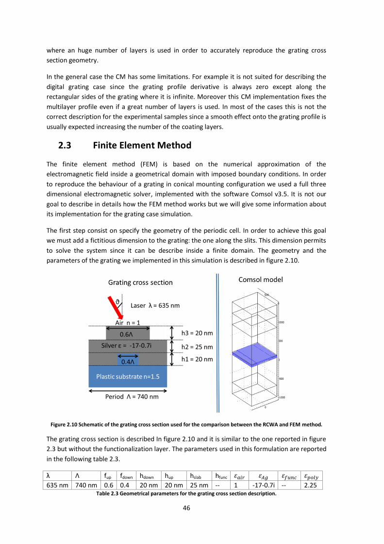
46
where an huge number of layers is used in order to accurately reproduce the grating cross
section geometry.
In the general case the CM has some limitations. For example it is not suited for describing the
digital grating case since the grating profile derivative is always zero except along the
rectangular sides of the grating where it is infinite. Moreover this CM implementation fixes the
multilayer profile even if a great number of layers is used. In most of the cases this is not the
correct description for the experimental samples since a smooth effect onto the grating profile is
usually expected increasing the number of the coating layers.
2.3 Finite Element Method
The finite element method (FEM) is based on the numerical approximation of the
electromagnetic field inside a geometrical domain with imposed boundary conditions. In order
to reproduce the behaviour of a grating in conical mounting configuration we used a full three
dimensional electromagnetic solver, implemented with the software Comsol v3.5. It is not our
goal to describe in details how the FEM method works but we will give some information about
its implementation for the grating case simulation.
The first step consist on specify the geometry of the periodic cell. In order to achieve this goal
we must add a fictitious dimension to the grating: the one along the slits. This dimension permits
to solve the system since it can be describe inside a finite domain. The geometry and the
parameters of the grating we implemented in this simulation is described in figure 2.10.
Figure 2.10 Schematic of the grating cross section used for the comparison between the RCWA and FEM method.
The grating cross section is described In figure 2.10 and it is similar to the one reported in figure
2.3 but without the functionalization layer. The parameters used in this formulation are reported
in the following table 2.3.
λ Λ fup fdown hdown hup hslab hfunc 휀𝑎𝑖𝑟 휀𝐴𝑔 휀𝑓𝑢𝑛𝑐 휀𝑝𝑜𝑙𝑦
635 nm 740 nm 0.6 0.4 20 nm 20 nm 25 nm -- 1 -17-0.7i -- 2.25 Table 2.3 Geometrical parameters for the grating cross section description.

47
The Comsol corresponding model is showed in figure 2.10 where the blue part represent the
silver layer. The domains above the silver layer represent the air meanwhile the ones below
represent the polycarbonate substrate.
In order to correctly solve the FEM model the incoming light polarization mode must be
specified. If the TM polarization mode is used the model has to be solved for 𝐻𝑥, 𝐻𝑦 since the
component perpendicular to the grating plane 𝐻𝑧 = 0. In each domain the refractive index must
be specified and the equation that will be solved is the Helmholtz equation for the Magnetic
field components:
∇ × (1
휀𝑟∇ ×𝑯)− 𝑘0
2𝑯 = 0 (2.44)
The upper and the lower domain are set as Perfectly Matched Layer adsorbing in the 𝑧-direction
since we want to avoid reflection due to the boundary condition. Along the sides of the periodic
cell we impose periodic boundary condition of Floquet type.
𝑯𝑑𝑠𝑡 = 𝑯𝑠𝑟𝑐exp (−𝑗𝒌(𝒓𝑑𝑠𝑡 − 𝒓𝑠𝑟𝑐)) (2.45) This equation means that the Magnetic field in the destination boundary 𝑯𝑑𝑠𝑡 must be the same
of the source 𝑯𝑠𝑟𝑐, except for a phase factor. Equation 2.45 forces the solution to be periodic
inside the unitary cell. In our case the periodicity momentum is defined by the vector 𝒌,
described in eq. 2.1.
We specify the input field by using the port boundary condition with a wave excitation of unitary
input power. The magnetic field has only the x, y component since we want to solve the problem
for a TM wave:
𝑯𝑖𝑛 = {
𝑠𝑖𝑛(𝜙)exp(−𝑗(𝑘𝑥𝑥 + 𝑘𝑦𝑥))
−𝑐𝑜𝑠(𝜙)exp(−𝑗(𝑘𝑥𝑥 + 𝑘𝑦𝑥))
0
(2.46)
And the propagation constant was set to 𝑘𝑧.
Inside the cell we impose continuity boundary condition. These ensure the continuity of the
tangential components of the electric and magnetic fields.
This method solves the magnetic field without using any Rayleigh development of the field. This
implies that the power of the various diffracted rays need to be directly calculated by using a
Fourier transform of the simulated fields.
The field in the substrate 𝑯𝒔 can be described as an expansion in the Rayleigh series as we have
already seen for the RCWA (eq. 2.6 ) and CM (eq. 2.23) methods. In fact:
𝑯𝒔(𝑧) =∑𝑯𝑚𝑛,𝑠 exp(−𝑖 [(𝑘𝑥 +𝑚2𝜋
Λ𝑥)𝑥
𝑚,𝑛
+ (𝑘𝑦 + 𝑛2𝜋
Λ𝑦)𝑦])exp (−𝑖𝑘𝑚𝑛,𝑠𝑧𝑧)
(2.47)
While in the upper region, ranging from the silver layer and the port boundary condition, the
upper field 𝑯𝒖 assumes the following form:

48
𝑯𝒖(𝑧) =∑𝑯𝑚𝑛,𝑢 exp (−𝑖 [(𝑘𝑥 +𝑚2𝜋
Λ𝑥)𝑥
𝑚,𝑛
+ (𝑘𝑦 + 𝑛2𝜋
Λ𝑦)𝑦])exp(−𝑖𝑘𝑚𝑛,𝑢𝑧𝑧)
+ 𝑐𝑯𝑖𝑛 exp (−𝑖𝑘𝑧(𝑧 − ℎ))
(2.48)
where 𝑐 = √2
Λ𝑥Λ𝑦
𝜀0
𝜇0
cos (𝜃)
𝜂𝑢 is a constant that imposes the unitary power to the port, ℎ is the 𝑧-
quote of the port interface, Λ𝑥, and Λ𝑦 are the dimension of the unitary periodic cell. The 𝑧
component of the diffracted ray momentum is:
𝑘𝑚𝑛,𝑢;𝑠𝑧 = √(𝜂𝑢;𝑠𝑘0)2− (𝑘𝑥 +𝑚
2𝜋
Λ𝑥)2
− (𝑘𝑦 + 𝑛2𝜋
Λ𝑦)
2
(2.49)
with the subscript 𝑢, 𝑠 referring to the upper medium and to the substrate, respectively. After
performing the Fourier transform of the 𝑯𝒔 or 𝑯𝒖 (subtracting the incident field component) we
can retrieve the component 𝑯𝑚𝑛,𝑠;𝑢 and use them in order to evaluate the diffracted rays
power:
𝑃𝑚𝑛,𝑠;𝑢 = Λ𝑥Λ𝑦2𝜂𝑢;𝑠
|𝑯𝑚𝑛,𝑠;𝑢|2√𝜇0휀0Re[cos (𝜃𝑚𝑛,𝑢;𝑠)] (2.50)
Where 𝜃𝑚𝑛,𝑢;𝑠 is the light output angle:
𝜃𝑚𝑛,𝑢;𝑠 = tan
−1
√(𝑘𝑥 +𝑚2𝜋Λ𝑥)2
+ (𝑘𝑦 + 𝑛2𝜋Λ𝑦)2
𝑘𝑚𝑛,𝑢;𝑠,𝑧
(2.51)
Some physical quantities, such as total reflectance, total transmittance, and absorptance of
silver layer, can be calculated by directly using Comsol built-in tools. With such tools, the net
power flows through any boundary can be easily calculated. This allows an immediate
calculation of the grating total transmittance and reflectance. The power dissipate by the silver
layer can be easily evaluated by means of Comsol integration tools by applying this formula:
𝑄 = ∫𝜔
2
𝑠𝑖𝑙𝑣𝑒𝑟 𝑑𝑜𝑚𝑎𝑖𝑛𝑠
𝐼𝑚(휀)|𝐸|2𝑑𝑉 (2.52)
We compared this FEM method with the RCWA one by calculating the diffraction efficiencies for
a grating with the cross section reported in figure 2.10.

49
Figure 2.11 Comparison between the reflectance parameters calculated by using the RCWA method (continuous line) and the FEM method (circle): (a) as a function of 𝜽, with 𝝓=0° and (b) as function of 𝝓, with 𝜽=45°. Both
calculated in the TM mode.
In Figure 2.11 we reported the comparison between the reflectance parameters Rtot, R0, and R-1
calculated by using the RCWA method (continuous line) and the FEM method (circle). In figure
2.11a we report the reflectance as a function of 𝜃, with 𝜙=0° meanwhile in figure 2.11b we
report the reflectance as function of 𝜙, with 𝜃=45°. As we can see there is a perfect agreement
between the RCWA and the FEM method.
We performed the same analysis for the transmittance of diffracted rays as can be seen in Figure
2.12. we compared the transmittance parameters Ttot, T0, and T-2 calculated by using the RCWA
method (continuous line) and the FEM method (circle). In figure 2.11a we report the reflectance
as a function of 𝜃, with 𝜙=0° meanwhile in figure 2.11b we report the reflectance as function of
𝜙, with 𝜃=45°. Also in this case we can see that there is a perfect agreement between the RCWA
and the FEM method.
Figure 2.12 Comparison between the Transmittance parameters calculated by using the RCWA method (continuous line) and the FEM method (circle): (a) as a function of 𝜽, with 𝝓=0°; (b) as function of 𝝓, with 𝜽=45°. Both
calculated in the TM mode.
Even if the simulation are the same for the RCWA and the FEM method, the latter is more
powerful because we can simulate every desired periodic structure, as we will see in section
0 10 20 30 40 50 60 700
0.1
0.2
0.3
0.4
0.5
0.6
0.7
0.8
0.9
1
refle
cta
nce
[a
.u.]
incident angle [deg]
= 0°
Rtot
R0
R-1
0 10 20 30 40 50 60 70 80 900
0.1
0.2
0.3
0.4
0.5
0.6
0.7
0.8
0.9
1
azimuthal angle [deg]
= 45°
Rtot
R0
R-1
continuous line = RCWA circle = FEM
b)
continuous line = RCWA circle = FEM
a)
0 10 20 30 40 50 60 700
0.02
0.04
0.06
0.08
0.1
0.12
0.14
0.16
tra
nsm
itta
nce
[a
.u.]
incident angle [deg]
= 0°
Ttot
T0
T-2
0 10 20 30 40 50 60 70 80 900
0.02
0.04
0.06
0.08
0.1
0.12
0.14
0.16
0.18
azimuthal angle [deg]
= 45°
Ttot
T0
T-2
continuous line = RCWA circle = FEM
continuous line = RCWA circle = FEM
b)a)

50
3.1.2. Moreover, thanks to the Comsol implemented tools, the fields inside the nanostructured
surface can be easily calculated. As already specified in the introduction of this chapter, two -
dimensional simulations can be performed also by using the RCWA and CM methods.
Nevertheless their codes implementation and convergence need a careful and dedicated
approach that will not be treated here.
2.4 Vector model method
We already introduced the vector model (VM) in section 1.2.2 applying it to the unidimensional
grating in the conical mounting configuration with 𝜙=0°. Here we want to generalize it to the
bidimensional periodic structure case, considering the conical mounting configuration.
Figure 2.13 schematic for the generalization of the Vector Model
A general bidimensional periodic structure, like a tilted chessboard, is reported in Figure 2.13.
The surface is invariant for every translation along any of the lattice vectors �⃗� = 𝑛1𝑎1⃗⃗⃗⃗ + 𝑛2𝑎2⃗⃗⃗⃗ is
performed. Being 𝑎1⃗⃗⃗⃗ , and 𝑎2⃗⃗⃗⃗ in reference to figure 2.13:
𝑎1⃗⃗⃗⃗ = {Λ1
Λ1tan (𝜓)0
; 𝑎2⃗⃗⃗⃗ = {0
Λ2cos (𝜓)0
(2.53)
The reciprocal lattice vectors could be found straight forward [69] by considering:
𝑔1⃗⃗⃗⃗ = 2𝜋(𝑎2⃗⃗⃗⃗ × 𝑒3⃗⃗ ⃗)
𝑎1⃗⃗⃗⃗ ∙ (𝑎2⃗⃗⃗⃗ × 𝑒3⃗⃗ ⃗); 𝑔2⃗⃗⃗⃗ =
2𝜋(𝑒3⃗⃗ ⃗ × 𝑎1⃗⃗⃗⃗ )
𝑎1⃗⃗⃗⃗ ∙ (𝑎2⃗⃗⃗⃗ × 𝑒3⃗⃗ ⃗) (2.54)
where 𝑒3⃗⃗ ⃗ is the unitary vector along the 𝑧-axis. This implies that the two dimensional plasmonic
equations 1.33 in the grating plane 𝑥, 𝑦 becomes:
�⃗� 𝑠𝑝𝑝 = 𝜂𝑑�⃗� 0;𝑔.𝑝. + [cos (𝜙) −sin (𝜙)sin (𝜙) cos (𝜙)
] (𝑚1𝑔1⃗⃗⃗⃗ + 𝑚2𝑔2⃗⃗⃗⃗ ) (2.55)
This equation is satisfied when:
sin(𝜃) = −𝜌𝑔 cos(𝜙 − 𝛽) ± √𝜌𝑠𝑝𝑝2 − 𝜌𝑔
2 sin2(𝜙 − 𝛽) (2.56)
where 𝜌𝑔 = |𝑚1𝑔1⃗⃗⃗⃗ ⃗+𝑚2𝑔2⃗⃗⃗⃗ ⃗|
𝜂𝑑𝑘0; 𝜌𝑠𝑝𝑝 =
𝑘𝑠𝑝𝑝
𝜂𝑑𝑘0, meanwhile 𝛽 = cos−1 [
(𝑚1𝑔1⃗⃗⃗⃗ ⃗+𝑚2𝑔2⃗⃗⃗⃗ ⃗)𝑥
|𝑚1𝑔1⃗⃗⃗⃗ ⃗+𝑚2𝑔2⃗⃗⃗⃗ ⃗|].

51
We can notice that the resonance has the same analytical form for one-dimensional or a bi-
dimensional periodic grating is used. In fact the one - dimensional grating is described by
equation 2.56 imposing 𝑚1 or 𝑚2 = 0. Moreover we underline that 𝛽 depends only on the
geometrical parameters, and not on the surface condition.
In the next chapter we will use this model to fit the plasmonic resonances obtained from the
periodic nanostructured surfaces simulation. Then we will see how this method can be used to
predict the sensitivity of various plasmonic configurations.

52

53
3 Simulation Results
In this chapter we will show the main results obtained by using the simulation tools previously
described. First we will analyse the results we obtained by lighting a nanostructured surface in
conical mounting configuration. We will start from the RCWA simulation of the one dimensional
grating [70]–[72]. Then, by means of the FEM method, we will analyse two-dimensional
nanostructures that can be considered as a superposition of two or three one dimensional
gratings. We will also see that the SPRs resonances are well fitted by the Vector Model.
Then we will study the characterization of the SPRs in the Kretschmann configuration for flat and
grating surfaces.
Moreover since the Kretschmann and grating coupling configurations excite the same surface
modes, we will undercover and discuss their common features.
Finally we will study the theoretical sensitivity of the SPRs. In each case the sensitivity will be
calculated by changing the refractive index of the dielectric medium, and by modeling a
dielectric thin layer that covers the metal part of the interface. We will perform this analysis
considering as possible variables: the wavelength, the incident angle, the polarization angle, and
the azimuthal angle.
3.1 Nanostructured surfaces in conical mounting
configuration
3.1.1 Grating
First of all we will study the behaviour of the grating in the conical mounting configuration by
considering the zero order reflectance (R0) and the total grating transmittance (Ttot). These are
the experimental quantities we can measure with our experimental set up. All the grating
simulations that we will show in this section are computed via the RCWA method. In reference
to figure 2.10 we will use the following grating cross section parameters:
λ Λ fup fdown hdown hup hslab hfunc 휀𝑎𝑖𝑟 휀𝐴𝑔 휀𝑓𝑢𝑛𝑐 휀𝑝𝑜𝑙𝑦
635 nm
740 nm
0.45 0.3 20 nm
20 nm
35 nm
-- 1 -17-0.7i
-- 2.4964
Table 3.1. Grating model parameters used in this section.

54
Figure 3.1 SPRs for a unidimensional grating in conical mounting configuration: (a) pairs (𝜽, 𝝓) calculated by using the VM, (b) R0 and (c) Ttot calculated by using the RCWA method, as a function of 𝜽 and 𝝓 for the TM polarization
mode
In figure 3.1a we report the resonance curves calculated via the vector model by using the
parameters reported in table 3.1. In figure 3.2b and 3.2c we report the parameters R0 and Ttot
calculated by lighting the grating in the TM mode. In all these figures the calculated quantities
are shown only for the positive azimuthal angles since they are symmetric respect to 𝜙 = 0°
axis.
As we can see the resonances shape follows the vector model curves and they are characterized
by a minima in R0, and a maxima in Ttot. If a cross section at 𝜙 = 0° of the total transmittance
map is considered, two maxima appear, corresponding to the SPR 𝑚=1 and 𝑚=-2, respectively.
Let us call these two critical points (𝜃𝑐,1; 𝜙𝑐,1) and (𝜃𝑐,−2; 𝜙𝑐,−2). If we analyse a 𝜃-cross
section of the Ttot map for 5° < 𝜃 < 𝜃𝑐,1, Ttot show only a maximum at 𝜙 = 0°. The value of this
maximum increases while 𝜃 becomes closer to 𝜃𝑐,1 and for 𝜃 = 𝜃𝑐,1 it reaches the highest value.
If a similar cross section is considered for 𝜃𝑐,1 < 𝜃 < 35.7° the two symmetric peaks at ±𝜙𝑟,1
appear. The absolute values of this resonance position 𝜙𝑟,1 increases augmenting 𝜃, and we can
also see that the peak transmittance decreases until it disappears for 𝜙 = 90°. A similar
behaviour of the azimuthal resonance can be noticed for the SPR 𝑚=-2; if a 𝜃-cross section of
the map for 35.7° < 𝜃 < 𝜃𝑐,2 the azimuthal transmittance has three maxima two a ±𝜙𝑟,−1 due
to the excitation of the SPR 𝑚=-1, and one at 𝜙 = 0° due to the 𝑚=-2 SPR. Considering now only
the resonances due to 𝑚=-2, if a cross section of the map is taken for 𝜃 > 𝜃𝑐,2, two azimuthal
resonances ±𝜙𝑟,−2 appear.
By comparing the R0 map with the Ttot map, and in particular the R0 minima and Ttot maxima, the
plasmonic resonances present the same behaviour. Nevertheless, fixed 𝜃, the azimuthal
resonance angle 𝜙𝑟, found as a minimum of the reflectance, is not exactly the found as a
maximum of the transmittance [73], [74]. We report in table 3.2 the azimuthal resonance angles
found through R0 and Ttot for the SPR 𝑚=1 and 𝑚=-2.
𝜙𝑟 SPR 𝑚=1; 𝜃 = 10.5° SPR 𝑚=-2; 𝜃 = 43.0°
R0 10.55° 4.00°
Ttot 10.30° 4.60° Table 3.2 Azimuthal resonance position found by using R0 and Ttot parameters for the SPR 𝒎=1 and 𝒎=-2.
[deg]
R0
0 20 40 60 800
10
20
30
40
50
60
70
80
90
[deg]
Ttot
0 20 40 60 800
10
20
30
40
50
60
70
80
90
0 20 40 60 800
10
20
30
40
50
60
70
80
90
Vector Model
[deg]
[deg]
m = 1
m = -1
m = -2
0.3
0.4
0.5
0.6
0.7
0.8
0.9
0.05
0.1
0.15
0.2
0.25
a) c)b)

55
As we can see from table 3.2 for the SPR 𝑚=1 the resonance angle found by using the R0
parameter is 0.25° greater than the one found considering the Ttot parameter. Conversely for the
SPR 𝑚=-2 𝜙𝑟 calculated through R0 is 0.6° lower than 𝜙𝑟 calculated by using Ttot.
Figure 3.2: (a) R0 and (b) Ttot calculated by using the RCWA method as a function of 𝜽 and 𝝓 for the TE polarization
mode
In figure 3.2a and 3.2b we report the parameters R0 and Ttot calculated for the grating lighted in
the TE mode as a function of 𝜃 and 𝜙, respectively. As for the TM case, the reported maps are
symmetric with respect to 𝜙 = 0° axis.
Also in this case the resonances follow the vector model and increase their amplitude with the
increasing their azimuthal angle, being strongest at 𝜙 = 90°. This behaviour is the opposite
respect to the resonances found in the TM mode. The SPR 𝑚=-2 resonance weakly excited
through this polarization mode, since it is confined for |𝜙| < 40°; in fact it is difficult to identify
it by looking at figure 3.2.
In conclusion, the plasmonic resonances for the unidimensional grating case appear as maxima
(minima) if Ttot (R0) parameter is plotted as a function of 𝜃 and 𝜙. The resonances shape follows
the curves predicted by using the Vector Model, and they appear as a sort of parabolic curve
𝜃(𝜙). This ⊂-shaped curves follow the analytical equation 2.56 of the vector model. The critical
points of the curves, i.e. the parabola vertexes, are represented by (𝜃𝑐,1; 0) and (𝜃𝑐,−2; 0) since
the azimuthal angle 𝛽 of the VM is geometrically forced to 0° (eq. 2.56, with 𝑚2=0). For each
resonance, the critical point strongly affects the azimuthal resonance behaviour. One single
azimuthal resonance is found at 𝜙= 0° if 𝜃 ≤ 𝜃𝑐 meanwhile two symmetric azimuthal resonance
can be identified for 𝜃 > 𝜃𝑐.
In the next section we will analyse two dimensional crossed gratings. They will produce
resonances described by the same analytical curves found for the one-dimensional grating case,
but with a critical point 𝜙𝑐 ≠ 0.
[deg]
[deg]
R0
0 20 40 60 800
10
20
30
40
50
60
70
80
90
[deg]
Ttot
0 20 40 60 800
10
20
30
40
50
60
70
80
90
0.2
0.3
0.4
0.5
0.6
0.7
0.8
0.9
0.05
0.1
0.15
0.2
0.25
a) b)

56
3.1.2 Two-dimensional nanostructures
The first Two-dimensional nanostructure we simulated through the FEM method is the one
showed in figure 3.3b. It is composed by two unidimensional gratings of 740 nm period rotated
by an angle of 20°. The nanostructure is therefore similar to an equilateral rhombus. The grey
areas describe the silver continuous layer which separates the substrate medium (glass,
𝜂𝑑 = 1.5) from the upper medium (air, 𝜂𝑑 = 1).The silver film thickness is set to 45 nm and the
nanostructure amplitude is 20 nm. We simulated the nanostructure with a TM polarized light
having a wavelength of 635 nm.
In figure 3.3a we report the total transmittance of the nanostructure and the position of the
resonances calculated by using the vector model (white dashed line). As we can see all the
different resonances due to the different SPR excitation orders, which in this case are described
by the two coupling number 𝑚1, and 𝑚2, are well reproduced in the region near the critical
point (𝜃𝑐; 𝛽). When two different orders should be excited for the same (𝜃,𝜙), some
plasmonics bandgap occurs and huge discontinuities in the transmittance map can be noted,
such as for 𝜃=16° and 𝜙= -55°.
Figure 3.3 (a) Ttot map as a function of 𝜽 and 𝝓 calculated for the bi-dimensional nanostructured surfaces by using a
635 nm light in the TM polarization mode. (b) schematic of the nanostructured surface.
As we can see the VM well reproduces the resonances calculated by means of the FEM method.
Hence the VM is the quickest and accurate instrument to use for calculate the angular position
of the SPR, when resonance shape and intensity are not required parameters. Also we can see
that the shape of the resonance does not change significantly if a more complex structure than
the one-dimensional grating, is used; we always obtain ⊂-shaped curves that follow the
analytical equation 2.56 of the vector model.
In the previous example, we compared the Ttot parameter calculated by the FEM method with
the curves produced by the VM. We found a good agreement between the two simulation
methods, being the transmittance maxima well fitted by the VM analytical curves. Nevertheless
the SPRs produced considering the previous case have a maximum coupling order |𝑚1,2|𝑚𝑎𝑥=2.
Hereafter we will study what happens when a coupling order up to |𝑚1,2|𝑚𝑎𝑥=6 could, in theory,

57
be excited and how the structure inside the periodic cell can affect the resonance coupling
strength.
In order to depict this aspect we calculated the transmittance map produced by the
nanostructures reported in figure 3.4
Figure 3.4 Different nanostructured surfaces implemented with the FEM method
Figure 3.4a represents the base bi-dimensional periodic structure we considered. In this case we
use two different periods being the shorter one 740 nm, meanwhile the longest one equals
2*1.3*740 nm. The other structures reported (3.4b, 3.4c, and 3.4d) are obtained by adding
another grating to the first nanostructure. For the structure reported in figure 3.4b, a grating is
added in the middle of the periodic cell halving the longest period that becomes in this case
1.3*740 nm. In figure 3.4c we added a grating parallel to the diagonal that goes from the upper
left corner down to the lower right corner. The opposite diagonal were used to add the grating
as it is reported in figure 3.4d. Like in the previous case the total film thickness was set to 45 nm
and the height of the nanostructure to 20 nm.
In figure 3.5 we report the Ttot maps found for the four different nanostructures (a, b, c, d)
shown in figure 3.4 as a function of (𝜃,𝜙) calculated using a 635 nm light in TM polarization
mode. White circles refers to the critical points (𝜃𝑐; 𝛽) we found by applying the VM to the
basic periodic cell described in figure 3.4a, since this is the cell that could be considered as the
unitary periodic cell for all the four cases here considered. As we can see from figure 3.5a, for
the simplest model considered, not all the critical points correspond to a vertex for a
transmittance ⊂-shaped resonance as conversely happens for the case reported in figure 3.3a.
This behaviour is typical also for the others nanostructured surfaces considered.

58
Figure 3.5 Ttot calculated for the nanostructured surfaces showed in Figure 3.4 the association follows the respective letters. The white circles refers to the critical points (𝜽𝒄; 𝜷) calculated by using the VM.
The total transmittance map noticeably changes If some geometrical features are added inside
the periodic cell, such as another grating with a fixed direction. This boosts some excitation
orders and weakens some others, e.g. the resonance that occurs at 𝜃𝑐=42.9° and 𝜙𝑐=0° of figure
3.5, corresponding to 𝑚1=2; 𝑚2=0, is stronger for the (a) and (b) geometries then it is weakened
by the (d) geometry and it disappears in the (c) geometry. There are also some resonances that
never appear such as the one at 𝜃𝑐=37.9°, 𝜙𝑐=70° which in this case corresponds to the
excitation order 𝑚1=0; 𝑚2=5, or the one at 𝜃𝑐=63.6°, 𝜙𝑐=-53.4° corresponding to 𝑚1=2; 𝑚2=5.
Where 𝑚1 and 𝑚2 were calculated by considering the structure of figure 3.4a as the unitary cell.
Nevertheless regarding the geometry (b) if we use the smallest possible periodic cell for the VM
calculations, all the resonance that appear are well fitted. In fact by considering the smallest
periodic cells the maximum excitation order allowed by the vector model is |𝑚1,2|𝑚𝑎𝑥=2 as it
happens in the case of figure 3.3a
In this study we learn that also complicated structures show the usual plasmonic resonance
effect described, If present, by the vector model analytical equation 2.56. The change of the
periodic cell geometrical features can lead to an enhancement of certain resonances whose
shape and intensity can be evaluate through the FEM method.
[d
eg
]
0 10 20 30 40 50 60 70 80
-80
-60
-40
-20
0
20
40
60
80
0 20 40 60 80
-80
-60
-40
-20
0
20
40
60
80
[deg]
[d
eg
]
0 10 20 30 40 50 60 70 80
-80
-60
-40
-20
0
20
40
60
80
[deg]0 20 40 60 80
-80
-60
-40
-20
0
20
40
60
80
0.02
0.04
0.06
0.08
0.1
0.12
0.14
0.16
0.18
0.2
d)
b)
c)
a)
Ttot
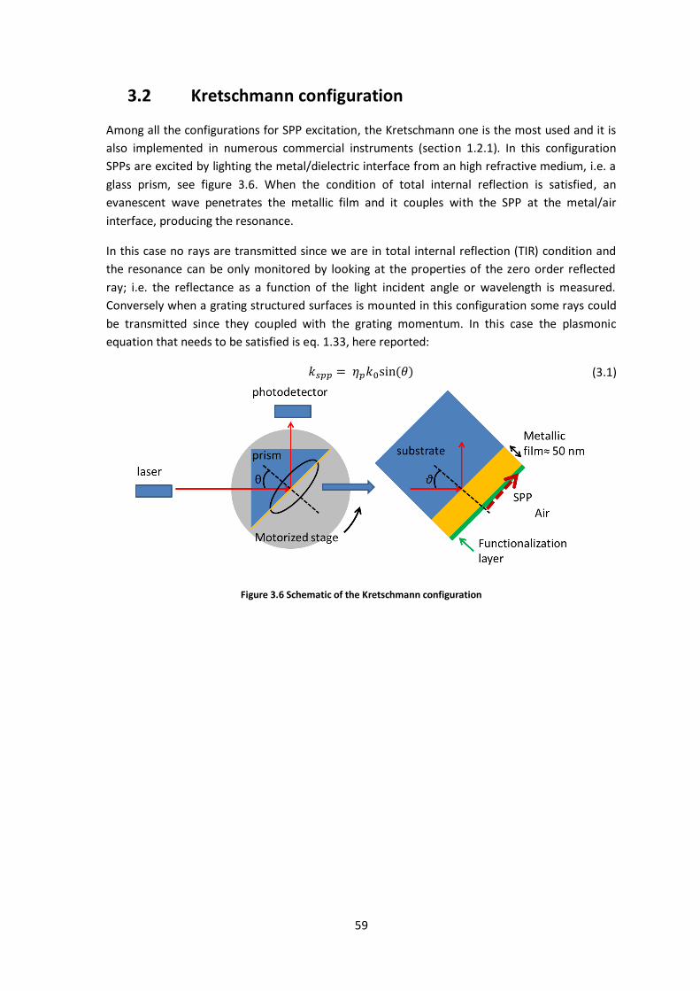
59
3.2 Kretschmann configuration
Among all the configurations for SPP excitation, the Kretschmann one is the most used and it is
also implemented in numerous commercial instruments (section 1.2.1). In this configuration
SPPs are excited by lighting the metal/dielectric interface from an high refractive medium, i.e. a
glass prism, see figure 3.6. When the condition of total internal reflection is satisfied, an
evanescent wave penetrates the metallic film and it couples with the SPP at the metal/air
interface, producing the resonance.
In this case no rays are transmitted since we are in total internal reflection (TIR) condition and
the resonance can be only monitored by looking at the properties of the zero order reflected
ray; i.e. the reflectance as a function of the light incident angle or wavelength is measured.
Conversely when a grating structured surfaces is mounted in this configuration some rays could
be transmitted since they coupled with the grating momentum. In this case the plasmonic
equation that needs to be satisfied is eq. 1.33, here reported:
𝑘𝑠𝑝𝑝 = 𝜂𝑝𝑘0sin (𝜃) (3.1)
Figure 3.6 Schematic of the Kretschmann configuration

60
3.2.1 Flat surfaces
We adopted the RCWA method to simulate the Kretschmann resonances, but we implemented a
simplified version of it, i.e. the one reported in the first part of Moharam work [52]. For the
characterization of this type of resonance we used a two layers system. The first layer represents
the silver film (yellow layer in Fig 3.6) and it is in contact with the polycarbonate substrate. The
second layer is placed between the silver metallic film and the air buffer (green layer in Fig 3.7).
This layer simulates the presence of a functionalization layer that will account for the biological
modification of the surface. The light, obviously, incomes from the polycarbonate substrate.
Initially we simulated the R0 map as a function of the incoming light incident angle and
wavelength. The parameters used in the simulation are:
𝜂𝑝=1.58 𝜂𝑎𝑖𝑟=1 𝜂𝑓𝑢𝑛𝑐=1 𝑑𝐴𝑔= 50 nm 𝑑𝑓𝑢𝑛𝑐= 1 nm Table 3.3 physical parameters used in the simulations
where 𝜂𝑝 is the polycarbonate refractive index which was assumed to be constant for all the
light wavelenght. Conversely the silver dielectric permittivity was considered as a function of the
wevelenght by using the values measured by Rakić [75].
We report in figure 3.7a R0 as a function of the incident light wavelength and the incident angle
found for a flat silver surface lighted in the TM mode. The SPR is clearly seen as the dark band
inside the map that represent the reflectance minima. In figure 3.8b we report R0 as a function
of 𝜃 for 𝜆 = 633 nm calculated with the same previous conditions. Here the resonance is a
represented by a sharp minimum in the R0 parameter. The experimental characterization of this
minimum will be discussed in section 4.2.2
Figure 3.7 R0 parameter calculated as a function of 𝜽 and 𝝀. (b) R0 as a function of 𝜽 for 𝝀=633 nm. Both figures were calculated for a flat silver surfaces lighted in the Kretschmann configuration with TM polarized light.
[deg]
[n
m]
R0
30 35 40 45 50 55 60400
500
600
700
800
900
1000
1100
1200
1300
1400
39 40 41 42 43 440
0.1
0.2
0.3
0.4
0.5
0.6
0.7
0.8
0.9
1
[deg]
R0 [a
.u.]
= 633 nm
0.1
0.2
0.3
0.4
0.5
0.6
0.7
0.8
0.9
b)a)

61
3.2.2 Grating surfaces
In the previous section we saw what happens when a flat metal/dielectric interface is lighted in
Kretschmann configuration. Now we want to study what happens when instead of flat surfaces
we light a unidimensional nanostructured surface. This field has been studied in other works in
order to understand the excitation of the SPP in the upper and lower interface [76], [77], and to
enhance the Kretschmann sensitivity [78], [79]. Nevertheless all these studies refer to the
condition where the grating is oriented perpendicular to the scattering plane i.e. 𝜙=0°. Here we
will study the complete system as a function of the 𝜃 and 𝜙 angles and we will show what
happens at the nanostructured metal/substrate interface and at the metal/dielectric one.
Figure 3.8 (a) Schematic of the excitation of SPP in the Kretschmann configuration using a nanostructured surface. (b) R0 as a function of 𝜽 and 𝝓 calculated using a unidimensional grating lighted in a Kretschmann configuration by
using a 633 nm light wavelength in TM polarization mode.
We schematized the results in figure 3.8a. The light was incoming from the grating
polycarbonate substrate and it was reflected from the silver yellow layer. The intensity of this
reflected ray is reported as a function of 𝜃 and 𝜙 in figure 3.8b, and were calculated assuming
that the grating is lighted with a 633 nm laser and in TM polarization mode. The grating
parameters were the ones reported in table 3.1. The Kretschmann plasmonic excitation
corresponds to the dark vertical band in figure 3.9b, fitted by the grey line. It relates to the
excitation of the SPP at the metal/air interface and it is independent from the azimuthal angle
since its excitation follows eq. 3.1.
At the polycarbonate/metal interface another SPP can be excite. This coupling could be related
to the 𝑚=-3 (red dashed line) or 𝑚=1 (red continuous line) orders. Also in these cases the SPP
excitation is represented by the classical vector model (eq. 2.56) considering the polycarbonate
refractive index 𝜂𝑑=1.58. As we can see, from figure 3.8b, shallow minima are present along the
red dashed line. Hence the weak coupling of the SPP at this interface should follow the SPR 𝑚=-3
order. We measured these plasmonic resonances in section 4.2.3 and we found that, despite
these simulations results, the most pronounced SPP excitation order is the 𝑚=1 one.
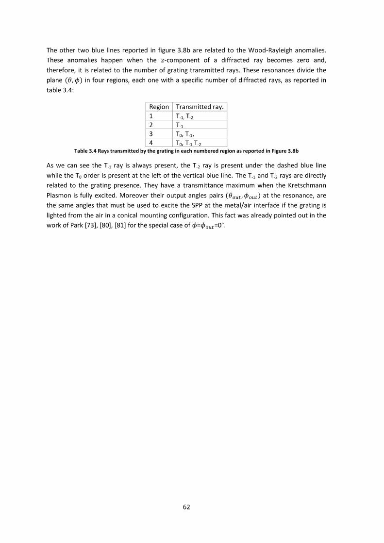
62
The other two blue lines reported in figure 3.8b are related to the Wood-Rayleigh anomalies.
These anomalies happen when the 𝑧-component of a diffracted ray becomes zero and,
therefore, it is related to the number of grating transmitted rays. These resonances divide the
plane (𝜃, 𝜙) in four regions, each one with a specific number of diffracted rays, as reported in
table 3.4:
Region Transmitted ray.
1 T-1, T-2
2 T-1
3 T0, T-1,
4 T0, T-1 T-2 Table 3.4 Rays transmitted by the grating in each numbered region as reported in Figure 3.8b
As we can see the T-1 ray is always present, the T-2 ray is present under the dashed blue line
while the T0 order is present at the left of the vertical blue line. The T-1 and T-2 rays are directly
related to the grating presence. They have a transmittance maximum when the Kretschmann
Plasmon is fully excited. Moreover their output angles pairs (𝜃𝑜𝑢𝑡 , 𝜙𝑜𝑢𝑡) at the resonance, are
the same angles that must be used to excite the SPP at the metal/air interface if the grating is
lighted from the air in a conical mounting configuration. This fact was already pointed out in the
work of Park [73], [80], [81] for the special case of 𝜙=𝜙𝑜𝑢𝑡=0°.

63
3.3 Relationship between the Kretschmann and grating
configurations
The main difference between the Kretschmann and the grating configuration is the excitation
medium. In the grating configuration the light incomes from the upper dielectric medium while
in the Kretschmann configuration it incomes from an high refractive index medium. Previously,
we showed that if the flat interface of the Kretschmann configuration is replaced with a
nanostructured surface there are also some transmitted rays that propagate in the dielectric
medium. When the Kretschmann plasmon is excited, these rays are transmitted with an angle
respect to the normal which is the same one that must be used to excite the SPP if the same
nanostructured surface is lighted in conical configuration [74].
Nevertheless the picture is not yet complete; here we will explain what happen to the grating
transmitted rays in the substrate when the grating is lighted in the conical configuration. We will
see that among all the four transmitted rays, propagating in the grating substrate, there is only
one that carries the major information about the SPR transmittance. At the maximum of the
excitation this ray propagates into the substrate with an angle that is equal to the one that must
be used to excite the SPP in the Kretschmann configuration [74]. Here we will analyse two
different cases: the transmitted ray when SPR 𝑚=1 in air is excited (figure 3.9 and following),
and when SPR 𝑚=-2 in water is excited (figure 3.10 and following).
We have already seen that in order to excite the SPP through a grating in the conical mounting
configuration the equation 2.56 must be satisfied. The equation is reported here for the simply
case of a unidimensional grating:
𝑠𝑖𝑛(𝜃𝑖𝑛) =
−𝑚𝐺𝑐𝑜𝑠(𝜙𝑖𝑛) ± √−𝑚2𝐺2 sin2(𝜙𝑖𝑛) + 𝑅𝑒
2(𝑘𝑠𝑝𝑝)
𝑘0𝜂𝑑
(3.2)
where 𝑘0 = 2𝜋/𝜆 is the vacuum light momentum and 𝜆 the vacuum wavelength, 𝜂𝑑 is the
refraction index of the dielectric medium (air or water), 𝑘𝑠𝑝𝑝 = 𝑘0√𝜀𝑑𝜀𝑚
𝜀𝑑+𝜀𝑚 is the modulus of the
SPP coupling constant, 휀𝑑 = 𝜂𝑑2 is the relative dielectric constant of the dielectric medium and
휀𝑚 is the metal dielectric constant, 𝐺 = 2𝜋/Λ, and Λ is the grating period. We add the subscript
𝑖𝑛 since we want to underline that these are the light incident angles in conical configuration
when the light propagates in the upper medium.
The output angle pair (𝜃𝑜𝑢𝑡,𝑛, 𝜙𝑜𝑢𝑡,𝑛) of the transmitted ray could be calculated through the
RCWA since their momenta components are:
{
𝑘𝑥,𝑛 = 𝑘𝑜[𝜂𝑑 sin(𝜃) cos(𝜙) + 𝑛(𝜆 Λ⁄ )]
𝑘𝑦 = 𝑘𝑜𝜂𝑑 sin(𝜃) sin(𝜙)
𝑘𝑧,𝑛,𝐼𝐼 = √(𝑘𝑜𝜂𝑝)2 − 𝑘𝑥,𝑛
2 − 𝑘𝑦2
(3.3)
Where 𝜂𝑝 is the refraction index of the polycarbonate grating substrate, and 𝑛 is the subscript
that corresponds to the Rayleigh - Floquet expansion order of the diffracted ray. The output
angle pairs is therefore:

64
𝜃𝑜𝑢𝑡,𝑛 = tan−1 (√𝑘𝑥,𝑛
2 + 𝑘𝑦2 𝑘𝑧,𝑛,𝐼𝐼⁄ ) ; 𝜙𝑜𝑢𝑡,𝑛 = tan
−1(𝑘𝑦 𝑘𝑥,𝑛⁄ ) (3.4)
In the two cases considered: air, and water, four transmitted rays T-2, T-1, T0, T1 are always
present.
Figure 3.9 (a) Ttot as a function of 𝜽𝒊𝒏 𝝓𝒊𝒏. (b) T-2, (c) T-1, (d) T0, (e) T1 as a function of 𝜽𝒐𝒖𝒕 𝝓𝒐𝒖𝒕, calculated for a
trapezoidal grating lighted in TM mode for the SPR 𝒎=1 in air. The black lines refer to the VM calculations
In figure 3.9a we report the Ttot as a function of 𝜃𝑖𝑛 and 𝜙𝑖𝑛. Here the same resonance of figure
3.1c can be seen and also in this case it is well fitted from the vector model considering 𝑚=1 as
the coupling constant. The transmittance values are slightly different because we use a
trapezoidal grating cross section. In reference to figure 2.8 the parameters used are reported in
table 3.5.
λ Λ fup fdown h dAg dfunc 휀𝑎𝑖𝑟 휀𝐴𝑔 휀𝑓𝑢𝑛𝑐 휀𝑝𝑜𝑙𝑦
635 nm 740 nm 0.75 0.93 20 nm 58 nm -- 1 -17-0.7i -- 2.4964 Table 3.5 Parameters used in the trapezoidal grating simulation
The other four figures 3.9b, 3.9c, 3.9d, and 3.9e show the ray transmittance T-2, T-1, T0, and T1
plotted as a function of their output angles (𝜃𝑜𝑢𝑡 , 𝜙𝑜𝑢𝑡), respectively. As we can see in all these
in
[deg]
in [deg]
Air SPR m = 1
7 8 9 10 11 12 13 14 15 16 170
20
40
60
80
Ttot
SPR m = 1
-90 -85 -80 -75
-8
-6
-4
-2
o
ut [
deg]
T-2
mp = 3
-30 -28 -26 -24
-15
-10
-5
6 8 100
20
40
60
80
out
[deg]
o
ut [
deg]
T0
mp = 1
38 40 42 440
5
10
15
out
[deg]
T1
mp = 0
0.02
0.03
0.04
0.05
0.06
0.07
0.08
1
2
3
4
5
6
7x 10
-4
0.0105
0.011
0.0115
0.012
0.0125
0.013
0.01
0.02
0.03
0.04
0.05
0.06
5
10
15
x 10-5
T-1
mp = 2
b) c)
a)
d) e)
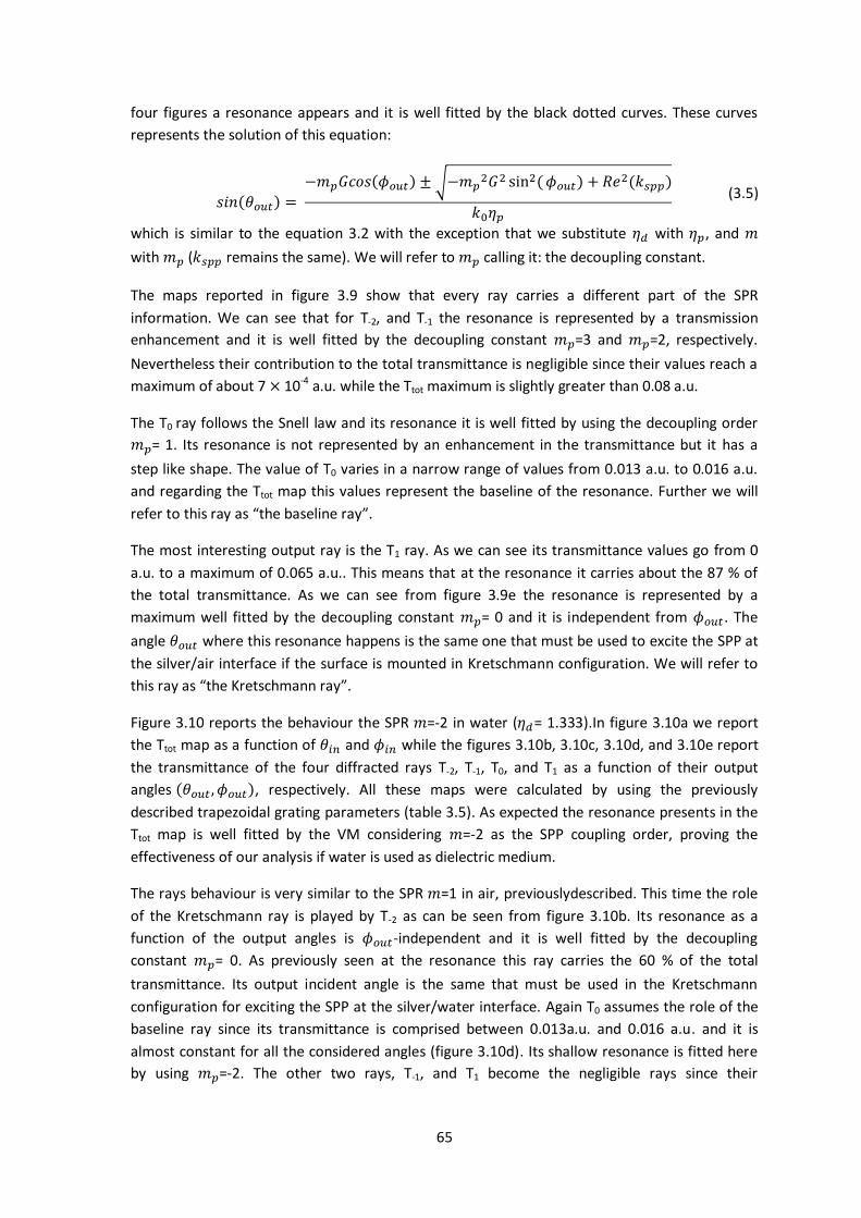
65
four figures a resonance appears and it is well fitted by the black dotted curves. These curves
represents the solution of this equation:
𝑠𝑖𝑛(𝜃𝑜𝑢𝑡) =
−𝑚𝑝𝐺𝑐𝑜𝑠(𝜙𝑜𝑢𝑡) ± √−𝑚𝑝2𝐺2 sin2(𝜙𝑜𝑢𝑡) + 𝑅𝑒
2(𝑘𝑠𝑝𝑝)
𝑘0𝜂𝑝
(3.5)
which is similar to the equation 3.2 with the exception that we substitute 𝜂𝑑 with 𝜂𝑝, and 𝑚
with 𝑚𝑝 (𝑘𝑠𝑝𝑝 remains the same). We will refer to 𝑚𝑝 calling it: the decoupling constant.
The maps reported in figure 3.9 show that every ray carries a different part of the SPR
information. We can see that for T-2, and T-1 the resonance is represented by a transmission
enhancement and it is well fitted by the decoupling constant 𝑚𝑝=3 and 𝑚𝑝=2, respectively.
Nevertheless their contribution to the total transmittance is negligible since their values reach a
maximum of about 7 × 10⁻⁴ a.u. while the Ttot maximum is slightly greater than 0.08 a.u.
The T0 ray follows the Snell law and its resonance it is well fitted by using the decoupling order
𝑚𝑝= 1. Its resonance is not represented by an enhancement in the transmittance but it has a
step like shape. The value of T0 varies in a narrow range of values from 0.013 a.u. to 0.016 a.u.
and regarding the Ttot map this values represent the baseline of the resonance. Further we will
refer to this ray as “the baseline ray”.
The most interesting output ray is the T1 ray. As we can see its transmittance values go from 0
a.u. to a maximum of 0.065 a.u.. This means that at the resonance it carries about the 87 % of
the total transmittance. As we can see from figure 3.9e the resonance is represented by a
maximum well fitted by the decoupling constant 𝑚𝑝= 0 and it is independent from 𝜙𝑜𝑢𝑡. The
angle 𝜃𝑜𝑢𝑡 where this resonance happens is the same one that must be used to excite the SPP at
the silver/air interface if the surface is mounted in Kretschmann configuration. We will refer to
this ray as “the Kretschmann ray”.
Figure 3.10 reports the behaviour the SPR 𝑚=-2 in water (𝜂𝑑= 1.333).In figure 3.10a we report
the Ttot map as a function of 𝜃𝑖𝑛 and 𝜙𝑖𝑛 while the figures 3.10b, 3.10c, 3.10d, and 3.10e report
the transmittance of the four diffracted rays T-2, T-1, T0, and T1 as a function of their output
angles (𝜃𝑜𝑢𝑡 , 𝜙𝑜𝑢𝑡), respectively. All these maps were calculated by using the previously
described trapezoidal grating parameters (table 3.5). As expected the resonance presents in the
Ttot map is well fitted by the VM considering 𝑚=-2 as the SPP coupling order, proving the
effectiveness of our analysis if water is used as dielectric medium.
The rays behaviour is very similar to the SPR 𝑚=1 in air, previouslydescribed. This time the role
of the Kretschmann ray is played by T-2 as can be seen from figure 3.10b. Its resonance as a
function of the output angles is 𝜙𝑜𝑢𝑡-independent and it is well fitted by the decoupling
constant 𝑚𝑝= 0. As previously seen at the resonance this ray carries the 60 % of the total
transmittance. Its output incident angle is the same that must be used in the Kretschmann
configuration for exciting the SPP at the silver/water interface. Again T0 assumes the role of the
baseline ray since its transmittance is comprised between 0.013a.u. and 0.016 a.u. and it is
almost constant for all the considered angles (figure 3.10d). Its shallow resonance is fitted here
by using 𝑚𝑝=-2. The other two rays, T-1, and T1 become the negligible rays since their
66
transmittance reaches a value of 2.2 × 10⁻⁴ a.u. meanwhile the Ttot maximum is slightly greater
than 0.06 a.u.. Their resonances are fitted by using 𝑚𝑝=-1 and 𝑚𝑝=-3, respectively.
Figure 3.10 (a) Ttot as a function of 𝜽𝒊𝒏 𝝓𝒊𝒏. (b) T-2, (c) T-1, (d) T0, (e) T1 as a function of 𝜽𝒐𝒖𝒕 𝝓𝒐𝒖𝒕 , calculated for a
trapezoidal grating lighted in TM mode for the SPR 𝒎=-2 in water. The black lines refer to the VM calculations
The analysis we performed here can be summarized in the following table for the SPR 𝑚=1 and
SPR 𝑚=-2, and it is valid for every dielectric medium in contact with the metal layer:
SPP 𝑚 = 1 SPP 𝑚 = -2
n mp DR mp DR
1 0 k -3 --
0 1 b -2 b
-1 2 -- -1 --
-2 3 -- 0 k Table 3.6 role of the n-th Rayleigh Floquet transmitted rays for the 𝒎 =1 and 𝒎 = -2 SPP coupling orders.
Table 3.6 summarizes the relation between the n-th diffracted order and the decoupling
constant mp we previously analyzed for the SPP excitation 𝑚=1 at the silver/air interface and for
the SPP 𝑚=-2 at the silver/water interface. Among all the transmitted rays, the Kretschmann ray
(mark in the table using “k”) carries most of the transmittance at the resonance condition. T0 is
in
[deg]
in [deg]
Water SPR m = -2
11 12 13 14 15 16 17 18 19 20 210
10
20
30
40
50
-70 -65 -60 -55
-14
-12
-10
-8
-6
-4
-2
o
ut [d
eg]
T-2
mp = 0
-25 -20 -15
-30
-25
-20
-15
-10
-5
T-1
mp = -1
10 12 14 160
10
20
30
40
50
out [deg]
o
ut [d
eg]
T0
mp = -2
44 46 48 50 52 540
5
10
15
out [deg]
T1
mp = -3
0.01
0.02
0.03
0.04
Ttot
SPR m = -2
0.013
0.014
0.015
0.016
0.5
1
1.5
2
x 10-4
1
2
3
4
5
x 10-5
0.02
0.03
0.04
0.05
0.06a)
b)c)
d) e)

67
the other important transmitted ray that influences the baseline transmittance value (has been
indicated with the “b”). The other two rays can be neglected due to the fact that their
transmittance is two orders of magnitude smaller respect to the transmittance carried by “k”
and “b” rays and they are marked in table with “--”.
The results reported in this table can be extended for other coupling orders but the main
features remains the same: the baseline ray follows the Snell law and carries the baseline
information having a shallow imprint of the resonance, meanwhile the Kretschmann ray carries
the greater part of the resonance information. In order to sense the transmittance of this ray
two possible methods could be experimentally pursued. In the first one the ray must be
extracted from the grating substrate by using an optically matched prism and then analyzed by a
light detector. In the second one optical medium continuity between the substrate and the
detector must be ensure. If these solutions are not implemented the Kretschmann ray will
undergo to TIR and it will not be sensed, losing the greater part of the SPR information. If this is
the case the only ray that will be sensed is the baseline one; nevertheless the resonance can still
be monitored as in Hiller’s work [82], [83].

68
3.4 Simulated sensitivity
In this section we will analyse how the SPR shifts can be exploited for sensing purpose in
different configurations. For each configuration we will see how these shifts are affected by a
dielectric refractive index (𝜂𝑑) increasing from 1 RIU to 1.02 RIU in step of 0.001 RIU. We will
also see how different thicknesses of a dielectric layer affect the resonance. Usually this
dielectric layer is used to simulate the presence of an organic layer (molecules, proteins, or
antibodies). We will simulate this functionalization layer by assuming that it is formed by a
dielectric having a refractive index of 1.5 RIU [20], [82], [84]. Its thickness will be varied from 0
nm to 10 nm in step of 0.5 nm.
Initially we will consider the wavelength and incident angle sensitivity for both the grating (𝜙=0°)
and Kretschmann configurations [16]. In the grating case we will also analyse how an azimuthal
rotation of the grating affect the 𝜃-sensitivity. In particular we will recall the azimuthal rotated
method introduced by Romanato [85]–[88], but we will also point out that an enhancement in
the 𝜃-sensitivity can be obtained exploiting the plasmonic excitation when the resonance curves
are almost parallel to the 𝜃-axis, i.e. for 𝜃>70° in figure 3.1.
Next, we will analyse the polarization sensitivity in the grating configuration applying it to the
case reported by Romanato [28], [89], [90] and to a condition adapts to our experimental
constrictions (light wavelength and grating geometry). Nevertheless we will see that the two
cases reach the same polarization sensitivity values.
Finally, we will introduce the azimuthal sensitivity which is one of the main parameters
developed in this work [91]. We will see that this sensitivity behaves like the double deep
incident angle sensitivity. Next we will improve this parameter by optimizing the shape of the
SPR curves.
For all the grating simulations we will use the digital grating cross section with the parameters
reported in table 3.1, meanwhile for the Kretschmann configurations we will use the parameters
of table 3.3. In all the figures reported seven different colours (from dark blue to brown) will
reproduce the curves we found for the different functionalization parameters. The colours will
refer to 𝜂𝑑 starting from 1.000 to 1.018 in step of 0.003 RIU if the buffer refractive index is
changed. If the functionalization study is performed the colours will refer to the functionalization
thickness going from 0 nm to 9 nm increasing in step of 0.15 nm.

69
3.4.1 Wavelength sensitivity
Grating configuration:
Figure 3.11 R0 map as a function of 𝜽 and 𝝀 calculated for 𝝓 = 0° lighting a grating in TM polarization mode. Black
and grey dashed curves refers to the VM calculation for 𝒎=-2 and 𝒎=1, respectively.
In figure 3.11 we report the R0 map as a function of 𝜃 and 𝜆 calculated for 𝜙=0° lighting the
grating with a TM polarized light. As we can see there are two intersecting dark bands. The one
marked with the black dashed line refers to the SPR 𝑚=-2 and the one marked with the grey
dashed line refers to the SPR 𝑚 =1. We can see that, when the two resonance cross each other,
a plasmonic bandgap appears similarly to what happens in the work of Alleyne [78]. Now we will
fix 𝜃 = 14° and we will analyse the behaviour of the 𝑚=1 SPR. In particular we will see what
happens to the plasmonic resonance when the dielectric medium refractive index 𝜂𝑑 (see figure
3.12a),or the functionalization layer thickness ℎ𝑓𝑢𝑛𝑐 (see figure 3.12b), increase.
Figure 3.12 Grating configuration: (a) R0 as a function of 𝝀 calculated increasing 𝜼𝒅, the inset shows the minimum position as a function of 𝜼𝒅, (b) R0 as a function of 𝝀 calculated increasing 𝒉𝒇𝒖𝒏𝒄, the inset shows the minimum
position as a function of 𝒉𝒇𝒖𝒏𝒄; both calculated with 𝜽 = 14°, 𝝓 = 0°, and in TM mode.
We report in figure 3.12a the curves R0 as a function of 𝜆 for 𝜃 = 14° and 𝜙 = 0° in TM mode
calculated for different values of 𝜂𝑑 as specified in the introduction of this section; going from 0
RIU to 0.018 RIU in step of 0.003 RIU. The reflectance minimum shifts toward higher values of 𝜆
with the increasing of the 𝜂𝑑 value. This shift is underline in the inset of figure 3.12a where we
[deg]
[nm
]
0 5 10 15 20 25 30 35 40 45 50450
500
550
600
650
700
R0
m = -2
m = 1 0.2
0.3
0.4
0.5
0.6
0.7
0.8
0.9
565 570 575 580 585 590 595 600 605 6100.2
0.3
0.4
0.5
0.6
0.7
0.8
0.9
1
[nm]
R0 [a.u
.]
1 1.01 1.02585
590
595
600
605
d [RIU]
m
in [n
m]
simulated
VM m = 1
565 570 575 580 585 590 595 600 605 6100.2
0.3
0.4
0.5
0.6
0.7
0.8
0.9
1
[nm]
0 5 10580
590
600
610
hfunc
[nm]
m
in [n
m]
simulated
VM m = 1
hfunc
d
b)a)

70
report the position of the minimum as a function of 𝜂𝑑 . The minima simulated with the RCWA
model is well fitted by the VM using 𝑚=1 and also a good linear relation between the minimum
position and the refractive index can be noted. The slope of this linear curve defined as 𝜕𝜆 𝜕𝜂𝑑⁄
= 660 nm/RIU is the wavelength sensitivity to the buffer variations and its value is similar to the
one of other grating coupling device as reported in [92]–[94].
Similarly we report in figure 3.12b the curves R0 as a function of 𝜆 calculated for different values
of ℎ𝑓𝑢𝑛𝑐as specified in the introduction of this section. The linear correlation between the
reflectance minima and the functionalization thickness is reported in the inset of figure 3.12b.
The slope of this linear curve defined as 𝜕𝜆 𝜕ℎ𝑓𝑢𝑛𝑐⁄ = 1.77 nmλ/nmfunc is the wavelength
sensitivity to the functionalization thickness variations.
Also in this case we can see a good correlations between the VM 𝑚=1 and the values simulated
by the RCWA code. In this case the relation between the two simulation methods is not well
specified as in the case of the buffer variation 𝜂𝑑 . In fact the parameter 𝜂𝑑 could be directly
inserted into the vector model, and its effect onto the plasmonic coupling 𝑘𝑠𝑝𝑝 constant is taken
into account by the definition of 휀𝑑 = 𝜂𝑑2 (eq 1.24). When we consider a functionalization layer
adsorbed onto the metallic surface we cannot change the buffer refractive index 𝜂𝑑but we must
change only the plasmonic coupling constant by changing 휀𝑑 = 𝜂𝑒𝑓𝑓2. The new defined
parameters 𝜂𝑒𝑓𝑓 is the effective refractive index and it considers the modification introduced by
the functionalization layer [20] since it is defined as:
𝜂𝑒𝑓𝑓 = 𝜂𝑑 +2ℎ𝑓𝑢𝑛𝑐𝑑𝑧
(𝜂𝑓𝑢𝑛𝑐 − 𝜂𝑑) (3.6)
where 𝜂𝑓𝑢𝑛𝑐 = 1.5 RIU is the refraction index of the functionalization layer and 𝑑𝑧 is the plasmon
penetration depth inside the dielectric medium defined in equation 1.27. In each case we will
consider 𝑑𝑧 as the parameter that allow us to reproduce the RCWA simulated resonance with
the Vector model.
We perform the same analysis for the SPR m = -2 taking 𝜃 = 33.5°. We found that 𝜕𝜆 𝜕𝜂𝑑⁄ =625
nm/RIU meanwhile 𝜕𝜆 𝜕ℎ𝑓𝑢𝑛𝑐⁄ = 0.9 nmλ/nmfunc, as reported in table 3.7.

71
Kretschmann configuration:
Figure 3.13 Kretschmann configuration: (a) R0 as a function of 𝝀 calculated increasing 𝜼𝒅, the inset shows the minimum position as a function of 𝜼𝒅, (b) R0 as a function of 𝝀 calculated increasing 𝒉𝒇𝒖𝒏𝒄, the inset shows the
minimum position as a function of 𝒉𝒇𝒖𝒏𝒄; both calculated with 𝜽 = 40.8° and in TM mode.
We perform the same analysis considering a flat surface in the Kretschmann configuration. In
figure 3.13a we report different curves of R0 as a function of 𝜆 for 𝜃 = 40.8° calculated for
different values of 𝜂𝑑 . A shift of the resonance as a function of the wavelength is clearly present
and it is reported in the inset of figure3.13a. As we can see the simulated minima are well
reproduced by the VM if used in the Kretschmann configuration (eq. 3.1). Nevertheless the
relation between the minima position and 𝜂𝑑 it is no longer linear and the buffer sensitivity goes
from 1.0 × 10⁵ nm/RIU to 3.9 × 10⁵ nm/RIU.
In figure 3.13b we report the curves of R0 as a function of 𝜆 calculated for different values of
ℎ𝑓𝑢𝑛𝑐. Again the minimum of the reflectance shifts toward higher values with ℎ𝑓𝑢𝑛𝑐 increasing,
as it is reported in the inset of the figure 3.13b. In this case the RCWA simulated reflectance
minima are not well reproduced by the vector model and 𝜕𝜆 𝜕ℎ𝑓𝑢𝑛𝑐⁄ = 12.7 nmλ/nmfunc. This
mismatch could be ascribed to the fact the parameter 𝑑𝑧 is considered constant in our
calculations. This assumption well represent the grating case, where the total shift of the
functionalization is ~15 nm, but not this one, where a huge shift of ~150 nm is registered.
FWMH
[nm]
𝜕𝜆
𝜕𝜂𝑑
[nm/RIU]
𝜕𝜆
𝜕𝜂𝑑𝐹𝑊𝑀𝐻
[1/RIU]
𝜕𝜆
𝜕ℎ𝑓𝑢𝑛𝑐[nmλ/nmfunc]
𝜕𝜆
𝜕ℎ𝑓𝑢𝑛𝑐𝐹𝑊𝑀𝐻[1/nmfunc]
SPR m =1 6 660 110 1.77 0.295
SPR m = -2 3 625 208 0.9 0.3
Kretschmann 70 2.5 × 10⁵ 3570 12.7 0.18 Table 3.7 Overview of the FWMH, Sensitivity, and FOM parameters found using 𝝀 as sensing parameter.
In the table 3.7 we summarize the sensitivity parameters evaluated using the R0 minima
wavelength as sensing parameter. We also introduce the Full Width Medium Height (FWMH)
parameter of the resonance. The FWMH is evaluated as the R0 deep width at the medium of its
amplitude value. Obviously, the sharper is the resonance, the smaller is the FWMH and more
easy will be the SPR shift detection. This fact could be described evaluating the Figure of Merit
(FOM) which is defined as the resonance sensitivity over its FWMH [16].
500 600 700 800 900 1000 1100 1200 1300 1400 15000.1
0.2
0.3
0.4
0.5
0.6
0.7
0.8
0.9
1
[nm]
R0 [a
.u.]
1 1.01 1.02600
700
800
900
1000
1100
d [RIU]
m
in [n
m]
simulated
VM
400 600 800 1000 1200 14000.1
0.2
0.3
0.4
0.5
0.6
0.7
0.8
0.9
1
[nm]
0 5 10650
700
750
800
850
hfunc
[nm]
m
in [n
m]
simulated
VM
hfunc
d
a) b)

72
We can see from the table 3.7 that if only the sensitivity is considered, the Kretschmann is the
best configuration since it has the highest sensitivity to 𝜂𝑑 and ℎ𝑓𝑢𝑛𝑐 . Otherwise, if the FOM is
taken into consideration, the Kretschmann configuration results the best choice for sensing 𝜂𝑑
variations, while the grating becomes the most appropriate configuration for detecting ℎ𝑓𝑢𝑛𝑐
changes.
3.4.2 Incident angle sensitivity
In this section we will study the incident angle sensitivity of the grating and Kretschmann
configurations. Exploiting the 𝜙-angle in the grating configuration we will see that the 𝜃-
sensitivity parameter can be enhanced reaching very high values.
Common configuration: grating with 𝜙=0°.
In figure 3.14a, and 3.14b we report the curves of R0 calculated as a function of 𝜃 for different
values of 𝜂𝑑 in the range 1 to 1.018 RIU, with a step of 0.003 RIU, calculated for the SPR 𝑚=1
and 𝑚=-2, respectively. In this case the grating is lighted by using 𝜆=635 nm, 𝜙=0° and TM
polarization. As we can see the two resonances have an opposite behaviour. In fact the
resonance shifts towards larger incident angles for SPR 𝑚=1, while it shifts towards lower angles
for the SPR 𝑚=-2. In both cases these shifts as a function of 𝜂𝑑 are well reproduced by the vector
model (see the corresponding insets). The same resonances shift behaviour is found if the
increasing of the functionalization thickness ℎ𝑓𝑢𝑛𝑐 is considered. The corresponding sensitivity
parameters, the FWMH, and the FOM are reported in table 3.8.
We want to underline that, since the SPR 𝑚=-2 (𝜃−2) shifts towards lower angles and the SPR
𝑚=1 (𝜃1) shifts to higher angles, the angular difference between the two dips Δ𝜃 = 𝜃−2 − 𝜃1
varies more than the singular resonance for the same 𝜂𝑑 variation. Effectively this method
enhance the angular sensitivity by adding the sensitivity values of the two resonance, since
𝜕Δ𝜃 𝜕𝜂𝑑⁄ = 𝜕𝜃−2 𝜕𝜂𝑑⁄ − 𝜕𝜃1 𝜕𝜂𝑑⁄ . This very simple method is already discussed in literature by
Cai [95] and it is referred as Double Dip Method (DDM).
Figure 3.14 Grating configuration: (a),(b) R0 as a function of 𝜽 calculated increasing 𝜼𝒅, the inset shows the minimum position as a function of 𝜼𝒅; both calculated with 𝝀 = 635 nm, 𝝓 = 0°, and in TM mode for the SPR 𝒎=1
and 𝒎=-2, respectively.
Kretschmann configuration:
8 10 12 14 16 180.2
0.3
0.4
0.5
0.6
0.7
0.8
0.9
1
[deg]
R0 [a.u
.]
38 40 42 44 46 480.78
0.8
0.82
0.84
0.86
0.88
0.9
0.92
0.94
[deg]
1 1.01 1.0210
10.5
11
11.5
d [RIU]
m
in [d
eg
]
simulated
VM m = 1
1 1.01 1.0240
41
42
43
d [RIU]
m
in [d
eg
]
simulated
VM m = -2
d
d
a) b)

73
Figure 3.15 Kretschmann configuration: (a) R0 as a function of 𝜽 calculated increasing 𝜼𝒅, the inset shows the minimum position as a function of 𝜼𝒅, (b) R0 as a function of 𝜽 calculated increasing 𝒉𝒇𝒖𝒏𝒄, the inset shows the
minimum position as a function of 𝒉𝒇𝒖𝒏𝒄; both calculated with 𝝀=633 nm and in TM mode.
In Figure 3.15a and 3.15b we report the R0 curves as a function of 𝜃 calculated by increasing the
parameter 𝜂𝑑 and ℎ𝑓𝑢𝑛𝑐, respectively. Both these figures were obtained by lighting the flat
surface in the Kretschmann configuration a λ = 633 nm light in TM polarization mode. We can
see that an increasing of the parameters 𝜂𝑑 or ℎ𝑓𝑢𝑛𝑐 causes a resonance minimum shift towards
higher incident angles likewise the 𝑚=1 SPR calculated in the grating configuration. The
sensitivity we found in this configuration is reported in table 3.8 and its values are very similar to
the one obtained for the SPR 𝑚=1.
Double Dip Azimuthally rotated method: grating with 𝜙 ≠0°.
Previously we exploited how the DDM can enhance the 𝜃-sensitivity. Nevertheless another
method to increase the 𝜃-sensitivity has been studied by the Romanato [85]–[87]. Since this
method is directly related to the azimuthal rotation of the grating respect to the light scattering
plane we will call this method Double Dip Azimuthally Rotated Method (DDARM).
Figure 3.16 (a) R0 as a function of 𝜽 and 𝝀 for 𝝓=63° lighted with a polarization angle 𝝍=140°. (b) R0 as a function of
𝜽 and 𝝓 lighted with 𝝀=855 nm in TM polarization mode (𝝍=0°). The grey dashed line refer to the VM calculations.
In figure 3.16a we report the R0 map as a function of 𝜆 and 𝜃 for the grating in conical mounting
configuration with 𝜙=63° and a polarization angle 𝜓 = 140°. The resonance is represented by a
dark band in the map and it is well reproduced by the VM 𝑚=1 (grey dashed line). The resonance
40 41 42 43 44 450.1
0.2
0.3
0.4
0.5
0.6
0.7
0.8
0.9
1
[deg]
R0 [a.u
.]
1 1.01 1.0241
41.5
42
42.5
d [RIU]
m
in [d
eg
]
simulated
VM
40 41 42 43 44 450.1
0.2
0.3
0.4
0.5
0.6
0.7
0.8
0.9
1
[deg]
0 5 1041
41.5
42
hfunc
[nm]
m
in [d
eg
]
simulated
VM
hfunc
a) b)
d
= 63°; = 140°
[deg]
[nm
]
0 10 20 30 40 50 60 70 80830
840
850
860
870
880
R0
m = 1
= 855 nm; = 0°
[deg]
[deg]0 10 20 30 40 50 60 70 80
50
52
54
56
58
60
62
64
66
68
70
R0
m = 1
0.55
0.6
0.65
0.7
0.75
0.8
0.85
0.9
0.95
0.5
0.55
0.6
0.65
0.7
0.75
0.8
0.85
0.9
0.95
a) b)

74
assumes a parabolic shape of 𝜃 as a function of 𝜆 and therefore if a cross section of the parabola
is considered for a fixed wavelength 𝜆<860 nm, two R0 minima at two different incident angles 𝜃
can be found. The light polarization angle (𝜓 = 140°) was chosen in order to obtain the same R0
values of these minima.
In figure 3.16b we report the R0 map as a function of 𝜃 and 𝜙 for the grating in conical mounting
configuration with 𝜆 = 855 nm. Here we can see that the main difference with the map reported
in figure 3.1b is that the resonance does not reach 𝜙=90° and neither the coupling order
changes its sign. This is due to the fact that the wavelength of the incident light is greater than
the grating period (740 nm).
The sensitivity enhancement of this method relays on the fact that the entire parabolic
resonance shape shifts towards higher values of lambda with the increasing of 𝜂𝑑 or ℎ𝑓𝑢𝑛𝑐 . The
effects of this shift is well explained by figure 3.17a and 3.17b where we report the curves of R0
as a function of 𝜃 for 𝜆=862 nm and 𝜓=140° obtained varying 𝜂𝑑 and ℎ𝑓𝑢𝑛𝑐, respectively. Since
we are lighting the grating with 𝜆>860 nm R0 has one single dip both for 𝜂𝑑=1 RIU and ℎ𝑓𝑢𝑛𝑐=0
nm. By increasing the parameter 𝜂𝑑 or ℎ𝑓𝑢𝑛𝑐 two dips appear and then their angular difference
increases.
We reported in the inset of the figures 3.17a and 3.17b the position of the minima (the ones at
higher angular position) as a function of 𝜂𝑑 and ℎ𝑓𝑢𝑛𝑐, respectively. As we see the vector model
well reproduces the resonances position, and the relation between 𝜃𝑚𝑖𝑛 and 𝜂𝑑 (or ℎ𝑓𝑢𝑛𝑐) is not
linear. Being the sensitivity represented by the slope of these curves, it diverges approaching the
condition where the two dips merge into a single one. This sensitivity behaviour as a function of
the parameters 𝜂𝑑 or ℎ𝑓𝑢𝑛𝑐 clearly depends on the fixed 𝜆. For example, if we want to tune the
high sensitivity region at higher values of 𝜂𝑑 (ℎ𝑓𝑢𝑛𝑐), we must increase the wavelength used.
This behaviour of the resonance sensitivity typically appears when a parabolic resonance shape
is exploited for sensing purpose. We will describe it in more details when we will discuss the
azimuthal sensitivity.
Even if the sensitivity diverge we reported in table 3.5 the maxima an the minima values we
found. In this case as FWMH we will use the width of the resonance considering its baseline
values the one it assumes at 𝜃=33°; nevertheless for a full description of the FOM problems in
this parabolic resonance case the reader can look to the experimental results in section 4.3.

75
Figure 3.17 DDARM method: (a) R0 curves as a function of 𝜽 calculated increasing 𝜼𝒅, the inset shows the minimum position at higher incident angle as a function of 𝜼𝒅, (b) R0 curves as a function of 𝜽 calculated increasing 𝒉𝒇𝒖𝒏𝒄, the
inset shows the minimum position at higher incident angle as a function of 𝒉𝒇𝒖𝒏𝒄; both were calculated with 𝝀=862
nm and with 𝝍=140°.
Single Deep Azimuthally rotated method: grating with 𝜙 ≠0°.
Figure 3.18 SDARM method: (a), (b) R0 curves as a function of 𝜽 calculated increasing 𝜼𝒅, the insets show the
minimum position at higher incident angle as a function of 𝜼𝒅, for the SPR 𝒎=-1 and 𝒎=-2, respectively.
In figure 3.18a and 3.18b we report the R0 curves as a function of the incident angle for
increasing values of the parameter 𝜂𝑑 for the SPR order 𝑚=-1 and 𝑚=-2, respectively. Also in this
case the grating was azimuthally rotated respect to the scattering plane using 𝜙=69° for the SPR
𝑚=-1 and 𝜙=32° for 𝑚=-2. The insets of the figure show the relation between the simulated
position of the resonance minimum and 𝜂𝑑 . Also in this case an excellent agreement between
the VM and the RCWA calculations can be noted. As we found for the case at 𝜙=0°, the two
resonances behave in two ways. For the SPR 𝑚=-1 the resonance angle increases with the
increasing of 𝜂𝑑; on the contrary for the SPR order 𝑚=-2 the minimum angle position decreases
with the increasing of 𝜂𝑑 . We can also notice that the relation between the minima position and
the 𝜂𝑑 is not perfectly linear, in particular for the SPR 𝑚=-2 case. If the parameter ℎ𝑓𝑢𝑛𝑐 is
0 10 20 30 40 50 60 70 80 90
0.5
0.6
0.7
0.8
0.9
1
[deg]
R0 [a.u
.]
1 1.01 1.0230
35
40
45
50
d [RIU]
m
in [d
eg
]
0 10 20 30 40 50 60 70 80 90
0.5
0.6
0.7
0.8
0.9
1
[deg]
0 5 1030
35
40
45
hfunc
[nm]
m
in [d
eg
]
simulated
VM m = 1
simulated
VM m = 1
hfunc
d
b)a)
70 75 80 85 90
0.65
0.7
0.75
0.8
0.85
0.9
0.95
1
[deg]
R0 [a.u
.]
60 65 70 75 80 85 900.84
0.86
0.88
0.9
0.92
0.94
0.96
0.98
1
1.02
[deg]
1 1.01 1.0273
74
75
76
77
78
d [RIU]
m
in [d
eg
]
simulated
VM m = -1
1 1.005 1.01 1.015 1.0260
65
70
75
d [RIU]
m
in [d
eg
]
simulated
VM m = -2
b) =69°, = 635 nm, = 0° =32°, = 635 nm, = 0°
a)
d
d

76
varied, instead of 𝜂𝑑 , the resonance behaviour is the same, and the sensitivity values we found
are reported in table 3.8.
The sensitivity enhancement obtained with this Single Deep Azimuthal Rotated Method
(SDARM) is also based on the parabolic resonance shape that can be seen in figure 3.1. These
resonances refers to the ∪ or ∩-shaped curves 𝜙(𝜃) that can be noticed for the SPR 𝑚=-1 and
𝑚=-2 if 𝜃>60°. In this case only half of the parabolic curves is present since 𝜃 cannot exceed 90°,
hence we are dealing with a single deep resonance. The resonance vertex has 𝜃=90° and its 𝜙
angle depends on the plasmonic resonance order being 68° for 𝑚=-1 and 33° for 𝑚=-2. Since the
resonance has a semi-parabolic shape its sensitivity can be enhanced by tuning the parameter 𝜙
assuming here the same role of 𝜆 in the DDARM. In this case a functionalization of the surface
causes a shift upward (downward) of the azimuthal coordinate of the parabolic vertex for the
SPR 𝑚=-2 (𝑚=-1). By accurately fixing 𝜙 one can tune the angular sensitivity. Nevertheless the
highest sensitivity configuration coincides with 𝜃=90° but this configuration is experimentally
unachievable.
FWMH [deg]
𝜕𝜃
𝜕𝜂𝑑
[deg/RIU]
𝜕𝜃
𝜕𝜂𝑑𝐹𝑊𝑀𝐻
[1/RIU]
𝜕𝜃
𝜕ℎ𝑓𝑢𝑛𝑐[deg/nm]
𝜕𝜃
𝜕ℎ𝑓𝑢𝑛𝑐𝐹𝑊𝑀𝐻[1/nm]
SPR 𝑚=1 0.6 55 91.6 0.14 0.23
SPR 𝑚=-2 0.8 -135 -168 -0.18 -0.23
Kretschmann 0.4 54 135 0.10 0.25
DDARM Max 2.5 2000 800 3 1.2
DDARM Min 5 500 100 1 0.2
SDARM 𝑚=-1 2 175 87 0.80 0.4
SDARM 𝑚=-2 3 -500 -166 0.74 0.24 Table 3.8 Overview of the FWMH, Sensitivity, and FOM parameters found using 𝜽 as sensing parameter.
Table 3.3 summarized the sensitivity parameters we found for the four different configurations
we simulated, considering 𝜃 as the sensing parameter.
As we can see, if 𝜙=0° (first three rows), the 𝜂𝑑 sensitivity for the SPR 𝑚=-2 is twice the one
retrieved for both the SPR order 𝑚= 1 and Kretschmann configurations. The sensitivity to the
parameter ℎ𝑓𝑢𝑛𝑐 is almost the same for all the three configurations.
A great improvement on the ℎ𝑓𝑢𝑛𝑐 and 𝜂𝑑 sensitivity is obtained by using the DDARM in its
region of sensitivity maximum. Here the sensitivity reaches values up to 2000 deg/RIU.
Considering also the FOM, this method seems to be the most suitable for plasmonic detection.
Also by using the SDRAM the sensitivity can be three times greater respect to the grating
measured at 𝜙=0°.
Both in the DDARM and SDARM methods the ability to enhance and tune the sensitivity
parameter is supported by the parabolic shape of the plasmonic resonance. This aspect will be
deeply analysed in section 3.4.4 and experimentally in section 4.3.

77
3.4.3 Polarization sensitivity
Another parameter that can be considered for sensing purpose is the polarization angle as
previously done by Romanato [28], [89], [90]. In this case the parameters 𝜆, 𝜃, 𝜙 will be fixed
and the only varying parameter will be the polarization angle 𝜓.
Figure 3.19: (a) R0 curves as a function of 𝝍 calculated increasing 𝜼𝒅, the inset shows the phase parameter 𝜶 as a function of 𝜼𝒅, (b) R0 curves as a function of 𝝍 calculated increasing 𝒉𝒇𝒖𝒏𝒄, the inset shows the inset shows the
phase parameter 𝜶 as a function of 𝒉𝒇𝒖𝒏𝒄; both were calculated with 𝝀=848 nm, 𝜽=43°, and with 𝝓=63°.
In figure 3.19a and 3.19b we will see how the curves of R0 as a function of 𝜓 are affected by the
increasing of the parameters 𝜂𝑑 and ℎ𝑓𝑢𝑛𝑐 , respectively. The incoming light parameters used
are: 𝜆=848 nm, 𝜃=43° and 𝜙= 63°. We notice that the shape of the curves is a classical harmonic
function:
𝑅0 = 𝐴 sin(2𝜋
180(𝜓 + 𝛼)) + 𝛿 (3.7)
Where 𝐴 represent the amplitude, 𝛿 the baseline, and 𝛼 the phase of the reflectance oscillation.
The relation between the curve phase 𝛼 and the parameter 𝜂𝑑 or ℎ𝑓𝑢𝑛𝑐 is reported in the insets
of the figure 3.19a and 3.19b. In this case the VM cannot reproduce these curve since the
incoming light polarizations is not considered in this model. Also in this case the relation is not
linear and in order to evaluate the 𝛼-sensitivity parameter we fitted the RCWA results with a
linear curve that will roughly reproduce the phase shift as a function of 𝜂𝑑 or ℎ𝑓𝑢𝑛𝑐. Usually for
low values of 𝜂𝑑 and ℎ𝑓𝑢𝑛𝑐 the 𝛼-sensitivity is almost 0 deg/RIU and then it increases. These
initial parameters (𝜆=848 nm, 𝜃=43° and 𝜙= 63°) were chosen in reference to figure 3.16a by
supposing that the initial grating condition 𝜂𝑑=1 RIU (ℎ𝑓𝑢𝑛𝑐=0 nm) lies on the parabolic
plasmonic resonance. The same analysis were performed considering different initial parameters
belonging to this parabolic 𝑚=1 SPR. The phase sensitivity results are reported in table 3.9.
Nevertheless the polarization sensing method does not need to be performed necessarily when
a parabolic shape of the resonance is present. In order to verify this we simulated the 𝛼-
sensitivity for our grating when: 𝜆=635 nm, 𝜃=59.5° and 𝜙= 74° as reported in figure 3.20. These
parameters were chosen in reference to figure 3.1b in order to exploit the polarization
behaviour of the order 𝑚=-1 SPR.
0 20 40 60 80 100 120 140 160 1800.5
0.55
0.6
0.65
0.7
0.75
0.8
0.85
0.9
0.95
1
[deg]
R0 [a.u
.]
1 1.01 1.02-30
-20
-10
0
10
d [RIU]
[d
eg
]
simulated
linear fit
0 20 40 60 80 100 120 140 160 1800.5
0.55
0.6
0.65
0.7
0.75
0.8
0.85
0.9
0.95
1
[deg]
0 5 10-10
-5
0
5
10
hfunc
[nm]
[d
eg
]
simulated
linear fit
a) b)
= 43°, = 848 nm, = 63° = 43°, = 848 nm, = 63°
d h
func

78
Figure3.20 (a) R0 curves as a function of 𝝍 calculated increasing 𝜼𝒅, the inset shows the phase parameter 𝜶 as a function of 𝜼𝒅, (b) R0 curves as a function of 𝝍 calculated increasing 𝒉𝒇𝒖𝒏𝒄, the inset shows the inset shows the
phase parameter 𝜶 as a function of 𝒉𝒇𝒖𝒏𝒄; both were calculated with 𝝀=635 nm, 𝜽=59.5°, and with 𝝓=74°.
In figure 3.20a and 3.20b we report the curves R0 as a function of 𝜓 for different values of 𝜂𝑑
and ℎ𝑓𝑢𝑛𝑐, respectively. From the insets of the figures 3.20a and 3.20b, that report 𝛼 as a
function of 𝜂𝑑 and ℎ𝑓𝑢𝑛𝑐 , we can notice the same behaviour registered in the precedent case,
even if this time the starting condition of the SPP excitation relays on the SPR 𝑚=-1 (see Figure
3.1b). Again, the behaviour of 𝛼 is not linear as a function of the functionalization parameters 𝜂𝑑
and ℎ𝑓𝑢𝑛𝑐 and a linear fit were used to roughly reproduce the resonance behaviour. Also in this
case we studied different initial conditions applied to this sensing technique.
The other cases we studied were chosen, in reference to figure 3.1. We selected the pairs:
𝜃=15.5° 𝜙=54°, 𝜃=51° 𝜙=22°, and 𝜃=64.5° 𝜙=30°, always with 𝜆=635 nm. The first pair refers to
the order 𝑚=1 SPR while the last two pairs refers to the order 𝑚=-2 SPR. We found that the 𝑚=-
2 SPR is not suited for this kind of sensing method, because the parameter 𝛼 as a function of 𝜂𝑑
and ℎ𝑓𝑢𝑛𝑐 is represented by a not-monotonic function. This implies that two different
functionalization parameters produce the same phase preventing the discrimination between
the two different surface conditions. For this reason we do not reported the results obtained for
SPR 𝑚=-2 in table 3.9.
𝜆 [nm] 𝜙 [deg] 𝜃 [deg] 𝑚 𝜕𝛼
𝜕𝜂𝑑 [deg/RIU]
𝜕𝛼
𝜕ℎ𝑓𝑢𝑛𝑐[deg/nm]
848 63 20 1 -480 -0.29
856 63 24.5 1 -765 -0.43
860 63 32 1 -1380 -0.82
856 63 39.5 1 -1670 -1.16
848 63 43 1 -1830 -1.54
635 54 15.5 1 -144 -0.25
635 74 59.5 -1 -2100 -5.50 Table 3.9 Phase polarization sensitivity found for different configurations
This sensing technique is possible only if 𝜙 ≠0° since the maximum excitation of the SPPs must
not happen in the TM polarization mode. An analytical expression for the polarization angle that
maximizes the excitation of the SPR resonance 𝜓𝑜𝑝𝑡 can be found in [28], [96] and it is:
0 20 40 60 80 100 120 140 160 1800.4
0.5
0.6
0.7
0.8
0.9
1
[deg]
R0 [a.u
.]
1 1.01 1.02-20
-10
0
10
20
d [RIU]
[d
eg
]
simulated
linear fit
0 20 40 60 80 100 120 140 160 1800.4
0.5
0.6
0.7
0.8
0.9
1
[deg]
0 5 10-40
-20
0
20
hfunc
[nm]
[d
eg
]
simulated
linear fit
hfunc
d
b)a) = 59.5°, = 635 nm, = 74° = 59.5°, = 635 nm, = 74°

79
𝑡𝑎𝑛(𝜓𝑜𝑝𝑡) = 𝑡𝑎𝑛(𝜙)cos (𝜃𝑟𝑒𝑠) (3.8)
where 𝜃𝑟𝑒𝑠 is the angle where the SPR resonance happen. From this equation we can guess that
a changes in the values of 𝜃𝑟𝑒𝑠 , due to a functionalization process, affect also the 𝜓𝑜𝑝𝑡
parameter which is proportional to 𝛼. This expression states also that if 𝜙 = 0° a change in the
𝜃𝑟𝑒𝑠 will not influence the 𝜓𝑜𝑝𝑡 parameter, hence this sensing method could be performed only
if 𝜙 is exploited.
As we can see from table 3.9 the sensitivity increases with the increasing of the light incident
angle. The sensitivity to the parameter 𝜂𝑑 reaches the same values (1830 ÷ 2100 deg/RIU) even
if the SPR coupling order 𝑚 change from 1 (5-th row) to -1(7-th row). Otherwise the sensitivity to
the parameter ℎ𝑓𝑢𝑛𝑐 is five time higher if 𝑚 is varied from 1 to -1 going from a value of -1.54
deg/nm to -5.50 deg/nm, respectively. The FOM and FWMH of these resonance were not taken
into consideration due to the harmonic shape of the function.
These results show that even if this method does not directly monitor the resonance position its
sensitivity could be comparable with the one found by using the DDARM. An exceptional high
sensitivity to the ℎ𝑓𝑢𝑛𝑐 parameter is found using the SPR 𝑚=-1 order.

80
3.4.4 Azimuthal angle sensitivity
The SPR shift can be analysed by monitor the 𝜙 angle once fixed the incident wavelength 𝜆 and
𝜃 [91]. In fact the resonance assumes a parabolic ⊂-shaped form if 𝜃 is considered as a function
of 𝜙, as we already seen in figure 3.1, both for the order 𝑚=1 and 𝑚=-2. Due to the parabolic
resonance shape this detection method has almost the same features we analysed for the
DDARM and SDARM methods.
Figure 3.21 Azimuthal method: (a)and (b) R0 curves as a function of 𝝓 calculated increasing 𝜼𝒅, the insets shows the minimum as a function of 𝜼𝒅, for the SPR 𝒎=1 and 𝒎=-2 respectively; both figures were calculated with 𝝀=635 nm
in TM polarization, and 𝜽=11° for the SPR 𝒎=1 and 42.5° for the SPR 𝒎=-2.
In figure 3.21a and 3.21b we report the curves of R0 as a function of the 𝜙 angle for different
values of 𝜂𝑑 and for the SPR 𝑚=1 and 𝑚=-2, respectively. We are lighting the grating with
𝜆 = 635 nm, and 𝜃 was set to 11° and 42.5° for the SPR 𝑚=1 and 𝑚=-2, respectively. Since in
this case we assumed TM polarized light the curves result symmetric respect to 𝜙=0°, hence we
report only the positive 𝜙 angles. The insets of the two figures report the position of the
resonance as a function of 𝜂𝑑 . We can notice a nonlinear relation between azimuthal resonance
position and 𝜂𝑑 nevertheless the simulated points are excellently fitted by the VM.
Noticeably, for the SPR 𝑚=1, if 𝜂𝑑 increases the azimuthal resonance position decreases, until
the two dips merge into a single one. Conversely for the SPR 𝑚=-2 a single large minimum is
initially present and then two dips appear with 𝜂𝑑 increasing. The azimuthal position of these
dips increases with the increasing of 𝜂𝑑 . In both cases the modulus of the sensitivity 𝜕𝜙 𝜕𝜂𝑑⁄
diverge as the azimuthal resonance approaches 𝜙=0°.
The same resonance behaviour is found if we increase the parameter ℎ𝑓𝑢𝑛𝑐. These features of
the resonances are very similar to the ones found for the DDARM and it is common when a
parabolic shape resonance is exploited for sensing purpose. Also in this case in order to analyse
the main features of this sensing method we reported in table 3.10 the maximum and minimum
sensitivity values we simulated.
0 5 10 15 20 25 30 35 40 450.2
0.3
0.4
0.5
0.6
0.7
0.8
0.9
1
[deg]
R0 [a.u
.]
0 5 10 15 20 250.8
0.82
0.84
0.86
0.88
0.9
0.92
0.94
[deg]
1 1.01 1.020
5
10
15
20
25
d [RIU]
m
in
simulated
VM m = 1
1 1.01 1.020
5
10
15
d [RIU]
m
in
simulated
VM m = -2
d
d
b)a)

81
FWMH [deg]
𝜕𝜙
𝜕𝜂𝑑
[deg/RIU]
𝜕𝜙
𝜕𝜂𝑑𝐹𝑊𝑀𝐻
[1/RIU]
𝜕𝜙
𝜕ℎ𝑓𝑢𝑛𝑐[deg/nm]
𝜕𝜙
𝜕ℎ𝑓𝑢𝑛𝑐𝐹𝑊𝑀𝐻[1/nm]
𝑚 =1 Max 3 -5750 -1920 -10.5 -3.5
𝑚 =1 Min 7.5 -1000 -133 -2 -0.27
𝑚 =-2 Max 1.5 3250 2170 3 2
𝑚 =-2 Min 2 500 250 1 0.5 Table 3.10 Overview of the FWMH, Sensitivity, and FOM parameters found using 𝝓 as sensing parameter
In the Table 3.10 we report the maximum and minimum values of sensitivity, we found by using
this detection technique. As we can see the sensitivity along with the FOM reaches very high
values, if considered in the region of the sensitivity maximum near 𝜙=0°. The maximum
sensitivity values reported are slightly higher than the one reported in Table 3.8 for the DDARM
model. Also in this case for a complete discussion of the FOM and FWMH behaviour the reader
should see section 4.3.
The features we will analyse hereinafter can be always applied when a parabolic resonance
shape is found i.e. for the DDARM, for the SDARM, for this azimuthal case and even for the V-
shaped resonance that can be seen in figure 3.11. We will take the azimuthal sensitivity as
example since it is the main argument of this work. In particular we will see how it is possible to
tune and enhance the sensitivity just by changing the light incident angle.
Figure 3.22 (a) Shift of the SPR m=1 curves in the 𝜽, 𝝓 plane increasing the 𝜼𝒅. (b) 𝝓 resonance position calculated
as a function of 𝜼𝒅 for fixed incident angles.
We report in Figure 3.22a what happens to the SPR m = 1, calculated with the VM, in the plane
𝜃, 𝜙 increasing the parameter 𝜂𝑑 . As we can see, increasing 𝜂𝑑 , the resonances curves shift to
higher 𝜃 values respect to the curve having 𝜂𝑑=1, changing in this way the 𝜃-coordinate of the
vertex position. Fixed an incident angle 𝜃 (vertical black dashed lines) the 𝜙-position of the
resonance is represented by the intersection between the vertical black dashed lines and the
resonance curves. The 𝜙-resonance as a function of 𝜂𝑑 are reported in figure 3.22b for the five
different 𝜃 angles. If a measurement with 𝜃 = 11.5° is performed the 𝜙-position of the
resonance decrease augmenting the parameter 𝜂𝑑 . Changing 𝜃 the 𝜙-position of the resonance
for each 𝜂𝑑 conditions changes and as well as the azimuthal variation Δ𝜙 between two
consecutive values of 𝜂𝑑 . This variation is maximized when the fixed 𝜃 corresponds exactly the
SPR parabola vertex. For example, if one consider the azimuthal variation between 𝜂𝑑=1.015 and
𝜂𝑑=1.020 for 𝜃 = 11.5° a ∆𝜙=-5° is achieved meanwhile if 𝜃 = 11.2° the ∆𝜙 is improved to -12°,
9.5 10 10.5 11 11.5 120
5
10
15
20
25
30
35
[deg]
[deg]
d =1.000
d =1.005
d =1.010
d =1.015
d =1.020
0 0.005 0.01 0.015 0.020
5
10
15
20
25
30
35
d [RIU]
= 11.5°
= 11.2°
= 10.9°
= 10.6°
= 10.2°
d
a) b) SPR m = 1

82
since 𝜃=11.2° is the parabola vertex calculated for the 𝜂𝑑=1.020 SPR curve (brown line in figure
3.22a).
The azimuthal sensitivity parameter 𝑆𝜙 =𝜕𝜙
𝜕𝜂𝑑 is related to the slope of the curves reported in
figure 3.22b. As we can see the slope is always negative and tends to diverge as the 𝜙-resonance
approaches 0°.
Figure 3.23 (a) Shift of the SPR m=-2 curves in the 𝜽, 𝝓 plane increasing the 𝜼𝒅. (b) 𝝓 resonance position calculated
as a function of 𝜼𝒅 for fixed incident angles.
The behaviour for the SPR 𝑚=-2 is reported in figure 3.23a. In this case the VM resonances
calculated in the plane 𝜃, 𝜙 shift to the left with the increasing of the parameter 𝜂𝑑 . This implies
that the 𝜃-coordinate of the parabolic vertex position decreases with the increasing of 𝜂𝑑 ,
contrarily to what happen for the SPR 𝑚=1 case. The 𝜙-resonance as a function of 𝜂𝑑 are
reported in figure 3.23b for the five different 𝜃-angles (black dashed line in figure 3.23a). If a
measurements with 𝜃 = 44.0° is performed the 𝜙-position of the resonance increases
augmenting the parameter 𝜂𝑑 . Also in this case changing 𝜃, the resonance 𝜙-position for each
𝜂𝑑 conditions changes as well as the azimuthal variation Δ𝜙 between each consecutive values of
𝜂𝑑 . This variation is maximized when the fixed 𝜃 is exactly the SPR parabola vertex. For example,
the azimuthal variation calculated considering 𝜂𝑑=1.000 and 𝜂𝑑=1.005 for 𝜃 = 44.0° is ∆𝜙=2°,
while if 𝜃=43.3° the ∆𝜙 is improved to 5.5°, since 𝜃=43.3° is the parabola vertex calculated for
the 𝜂𝑑=1.000 SPR curve (the dark blue curve in figure 3.23a).
The azimuthal sensitivity parameter 𝑆𝜙 is always positive and tends to diverge as the 𝜙-
resonance approaches 0°.
In conclusion, if a plasmonic resonance has a parabolic shape it can be used for enhance and
tune the sensitivity. In the general case, the parabolic resonance could be approximated in its
vertex by the following curve:
𝜌(𝜎)~ 𝜌𝑐 + 𝐾(𝜎 − 𝜎𝑐)2 +ℴ[(𝜎 − 𝜎𝑐)
4] (3.8)
where the parameter 𝜎𝑐 does not change as a consequence of a functionalization process while
the parameter 𝜌𝑐 is affected by the resonance. Fixed 𝜌, the resonance is monitored as a function
of 𝜎 and the sensitivity 𝑆𝜎 =𝜕𝜎
𝜕𝜂𝑑 can be maximized imposing 𝜎 = 𝜎𝑐.
41 42 43 44 45 46 470
5
10
15
[deg]
[deg]
d =1.000
d =1.005
d =1.010
d =1.015
d =1.020
0 0.005 0.01 0.015 0.020
5
10
15
d [RIU]
= 44.0°
= 43.3°
= 43.9°
= 42.4°
= 41.9°
a) b)
d
SPR m = -2

83
Method 𝝆 𝝈
DDARM 𝜆 𝜃
SDARM 𝜙 𝜃
Azimuthal 𝜃 𝜙
-- 𝜆 𝜙 Table 3.11 Different configurations where a parabolic resonance shape can be used.
In table 3.11 we report some different configurations where a parabolic resonance shape cab be
used in order to enhance and tune the sensitivity. The one represented in the last row was not
treated here but it is a possible configuration, since solving the VM as a function of 𝜆 and 𝜙 one
can find a parabolic shape resonance.
Even if 𝑆𝜎, in the case of parabolic resonance shape could diverge, this method applied to a
functionalization event can produce a maximum shift of the resonance condition:
|𝛥𝜎|𝑚𝑎𝑥 = √|𝛥𝜌
𝐾| (3.9)
where 𝛥𝜌 = 𝜌𝑓𝑢𝑛𝑐 − 𝜌𝑏𝑎𝑟𝑒 and 𝛥𝜎 = 𝜎𝑓𝑢𝑛𝑐 − 𝜎𝑏𝑎𝑟𝑒 and the subscript bare and func represent
the unmodified metallic surface and the functionalized metallic surface. If 𝐾 → 0 the parameter
|𝛥𝜎|𝑚𝑎𝑥 diverges. Obviously it is not possible to reach 𝐾~0 conditions since some optical effect
will prevent this i.e. the appearances of some Wood-Rayleigh modes.
If we consider the azimuthal method case the parameter 𝐾~𝑡𝑎𝑛( 𝜃𝑐) directly depends on the 𝜃-
vertex position. We found through simulation that to detect a refractive index variation
Δ𝜂𝑑=0.001 RIU, 𝜃𝑐 ≥0.8 must be used and a maximum shift of the azimuthal resonance of 20° is
calculated, reaching a sensitivity up to 2 × 10⁴ deg/RIU.

84

85
4 Experimental Results
In this chapter we will see some main results we obtained in plasmonic sensors characterization.
We will describe the two optical benches we used to excite the SPP for the grating and the
Kretschmann configurations.
Afterwards we will characterize the grating transmittance parameter Ttot when the
nanostructure is lighted in conical mounting configuration, and the parameter R0 if the same
nanostructured grating is mounted in Kretschmann configuration. Also the flat surface will be
characterized in Kretschmann configuration and the experimental results will be compared with
the simulated ones.
Then we will focus on the grating azimuthal sensitivity, changing the parameter 𝜂𝑑 and
ℎ𝑓𝑢𝑛𝑐.The parameter 𝜂𝑑 will be varied by using different water/glycerol solutions while for
increasing the ℎ𝑓𝑢𝑛𝑐 parameter, functionalization layers of different thicknesses adsorbed onto
the surface will be used.
Finally we will see the SPR shift produced when an antibody layer is immobilized onto the
grating surface exploiting both the 𝜙-sensitivity in the grating configuration and the 𝜃-sensitivity
in the Kretschmann configuration.
4.1 Experimental methods
In this section we describe the two optoelectronic benches we used to perform the
characterization of the SPRs. We illustrate the optoelectronic components we used and the
Labview© v8.6 implemented algorithms for the data acquisition.
4.1.1 Conical mounting configuration bench
Figure 4.1 Optoelectronic bench used for the excitation of the grating coupled SPR in conical mounting configuration, R0 sensing configuration. Upper inset Ttot sensing configuration, Lower inset: grating with the
microfluidic cell.

86
Figure 4.1 shows the opto-electronical bench for the conical mounting configuration [74]. This
optical bench allows to change both 𝜃 and 𝜙.
The light source is a solid-state laser diode (VHK model, Edmund Optics) with 635 nm
wavelength. The incident angle 𝜃 is fixed using a rotation stage (SL 20 model, Thorlabs) with a
full 360° angular sweep and a resolution of 2°. In order to accurately vary 𝜃, the laser is mounted
on a goniometer (GNL18 model, Thorlabs) with a range of 10° and a resolution of 10’.The laser
beam is polarized in the Transverse Magnetic (TM) mode. In order to vary the φ-angle a
motorized rotation stage (PRM1Z8 model, Thorlabs), mounted on a x-y translation stage
(ThorlabsDT25/M, Edmund Optics 56-795) is used. The photodiodes we used is an Hamamatsu
S1337 1010BR. We choose this photodiode because it has an high photosensitive area of 10 x 10
mm2, an high photosensitivity of 0.4 A/W, and a low dark current 200 pA.
If we want to monitor the R0 parameter the photodiode is mounted above the grating device as
we can see from figure4.10. When the transmittance is monitored, a photodiode is mounted on
a custom socket as can be seen in the upper right inset of figure 4.1. Measuring the two
quantities simultaneously, does not bring any advantage in term of the SPR detection
improvement since for a fixed 𝜃 the azimuthal resonance does not occur at the same 𝜙 as
previously discussed in section 3.1. When the Ttot parameter is measured the grating substrate
must be optimally coupled with the photodiode window through an optical matching oil (Cargille
Immersion Oil Type A) with 1.51 refraction index. This allows the correct propagation of the
Kretschmann ray from the polycarbonate substrate to the photodiode sensitive are, and hence
the correct detection of the plasmonic resonance, as we analysed in section 3.3.
In order to read the transmitted light signal intensity the photodiodes are connected to a
parameter analyzer (HP 4156B), which applies a constant bias of -2V to the photodiodes and
acquires the modulated current. By using this instrumental configuration we obtain a linear
relation between the measured current and the light intensity. We also used this optical bench
to monitor the kinetic behaviour of the azimuthal signal when the grating surface is exposed to
different liquid solutions. We achieved this by applying a microfluidic cell on the top of the
grating surface (lower right inset of figure 4.1) and connecting it with a peristaltic pump in order
to control the solution flux.
Our typical measurement consists in the acquisition of the current as a function of 𝜙, with a
fixed 𝜃. The currents measured when the grating is present are normalized by the current
measured when the laser directly hits the photodiode, in order to calculated Ttot or R0
parameters. We implemented two software for measuring the SPR resonance. The first one is
optimized for the acquisition of the complete resonance curve, acquiring the Ttot or R0
parameters while 𝜙 is continuously varied through the motorized rotation stage. The second
one is optimized for the measurement of the resonance kinetics due to functionalization
modifications that occurs at the metal/dielectric interface. We will briefly describe the
developed software by mean of their block diagrams and interface.
We report the block diagram of the first software in figure 4.2, left part, and a screenshot of the
software in the right part. First of all, the users must insert the start (𝜙𝑠), and stop (𝜙𝑒) angles of
the measurement. Then the angular velocity 𝜔 of the motorized stage and a parameter 𝛿 must
be inserted; usually they are set to 1 deg/sec and 0.05 deg. When the procedure starts, the

87
software sets the motorized rotation stage at 𝜙 < 𝜙𝑠 and then the rotation starts. When 𝜙𝑠 is
reached, the motorized rotation stage completes its acceleration process, and its angular
velocity is now constant. When the motorized rotation stage moves, we continuously measure
its position 𝜙𝑚, and if it satisfies the first condition block |𝜙𝑚 − 𝜙𝑠| < 𝛿, the current
measurement starts. The current measurement ends when |𝜙𝑚 − 𝜙𝑒| < 𝛿. Hence 𝛿 defines the
angular interval where the measurement starts and stops.
Figure 4.2 Block diagram and software interface for the acquisition of the complete resonance curve for the grating
lighted in conical mounting configuration.
When the motorized rotation stage stops we retrieve the current measured from the parameter
analyzer and we relate these values to the corresponding angular position, by using the
following formula:
𝜙 = 𝜙𝑠 +(𝜙𝑒 − 𝜙𝑠)
𝑁[0: 1:𝑁 − 1] (4.1)
where 𝑁 is the number of measurement performed by the parameter analyzer. Obviously, the
angular sampling frequency depends on the angular velocity of the motorized stage, if the
parameter analyzer one is fixed. For 𝜔 = 1 deg/sec we obtain an angular sampling frequency of
25 samples/deg. The instrument sampling frequency is fixed because we decided to use for each
measured current values an integration time of 20 ms which is equal to the power supply grid
period. In this way we avoide to pick up the 50 Hz noise coming from external sources.
As we can see from the software panel in figure 4.2 the measurements are not symmetric
respect to the zero of the motorized angle due to a sample misalignment respect to the
scattering plane that occurs during its positioning onto the socket. Nevertheless this error is
easily corrected exploiting the peak symmetry respect to 𝜙=0°. A shift of the measured curve in
order to obtain two opposite azimuthal peaks must be performed. The shape of the resonance
could appear wrong, but this is due to the fact that the current is reported with its sign. If the
modulus of the current is taken into consideration, the resonance appears as minima for the
reflectance, and as maxima for the transmittance.

88
We have also taken into account the effect of a possible delay between the validation of the
start and stop conditioning blocks and the effectively start and stop of the HP4156
measurement. Effectively this seem to be negligible for low 𝜔 as it is in our case but needs to be
considered for 𝜔 > 5 deg/sec.
We also include this software in a cycle that allows to repeat the measurement for the desired
number of times. The resonances measured for each different acquisition are reported by yellow
and blue curves reported in the lower panel of the software interface. The yellow and blue
curves refer to the azimuthal resonance as a function of the acquisition time calculated by using
the Ttot and R0 signals, respectively. As already found in our simulation (section 3.1) a constant
bias of 0.2° is found between the two measured resonance angles.
Figure 4.3 Block diagram and software interface for the acquisition of the SPR kinetics for the grating lighted in conical mounting configuration.
We developed a second software optimized for the kinetics measurement of the plasmonic
resonance as a function of the time (Figure 4.3). This software records the azimuthal peak
position meanwhile the condition of the metal/dielectric interface changes allowing to monitor
the molecular adsorption (see figure 4.24 and following) or the bio-recognition process.
Initially the motor angle of the azimuthal resonance peak 𝜙𝑠 must be inserted and 𝛿 is fixed
to0.2°. The motor moves at step of 𝛿 starting from an angular position of 𝜙𝑠 − 5𝛿 until it
reaches 𝜙𝑠 + 5𝛿. In the meantime during the motor movement the current is measured
producing a step like functions that could be seen in the two upper panels of the software
interface. Then, from the measured currents and the motor angular sweep, the new angular
resonance position 𝜙𝑟 is retrived. If the new resonance 𝜙𝑟 lies in the centre of the previous
sampling interval (|𝜙𝑠 −𝜙𝑟| < 3𝛿), the parameter 𝛿 is halved; if not, it is doubled. This allows
the software to follow the resonance if it is moving, and also to measure it accurately if a new
stable condition of the surface is reached. Nevertheless 𝛿 could not exceed the value of 0.4° or
be lower than 0.0125°. The software registers the resonance position and the current until the
user stops the software execution. Moreover the users need to choose which parameter, R0 or
Ttot, will be used to evaluate the resonance since, as we previously seen, they have a slightly
different azimuthal positions.

89
4.1.2 Kretschmann configuration bench
In figure 4.4 is reported a schematic of the Kretschmann bench we used [97], and in the inset its
picture. The laser source is an Helium-Neon laser HLN100LR (Thorlabs) of 10 mW power. The
laser spot is spatially filtered and polarized in the TM mode. The light enters into an NBK7 right
angle prism which is mounted on a motorized rotation stage. The reflected light is collected by a
photodiode (PDA-100-A-EC). The photodiode support is connected to another motorized stage
which is coaxial with the prism one. When the prism stage moves of a step Δ𝜃 the photodiode
stage moves of a 2Δ𝜃 step in order to capture the reflected ray power. The flat surface is
mounted on the hypotenuse of the prism and here it is optically coupled by using optical
matching oil (Cargille Immersion Oil Type A) with 1.51 refraction index.
Figure 4.4 (left) schematic of the optoelectronic bench used for Kretschmann configuration, (right) picture of the
optoelectronic bench.
The correct position of the prism relatively to the centre of the motorized rotation stage is
ensured by the white socket that holds the prism. This socket minimizes the area of the
metal/dielectric interface explored by the laser spot during an angular scan.
Figure 4.5 (a) Schematic of the ray propagation inside the prism and polycarbonate substrate, supposing that the prism rotation axis is R (star marked point) . (b) Maximum sweep of the parameter dA as a function of the rotation
axis position (Rx, Ry).

90
The calculus of optimal axis position in order to minimize the spot laser sweep (dA) as a function
of the prism angle was already treat by Qui [98] and we applied it to our case. The schematic of
the prism along with the polycarbonate substrate is reported in figure 4.5a. For simplicity, we
neglect the presence of the optical matching oil. Fixed the rotation axis position R=(Rx, Ry),
marked in the figure4.5a with a star, and the angle of the motorized stage 𝜃4 it is possible to
perform the geometrical ray tracing. In this way we can calculate the position of the point A as a
function of 𝜃4. Our goal is to find the position R that minimizes the maximum sweep of dA
calculated for 𝜃4 going from -30° to 30° in step of 5°.
The results are reported in figure 4.5b where we can see that for some Rx and Ry the minimum
sweep of dA reaches 0.4 mm.
Figure 4.6 Ray tracing of the light inside the prism and polycarbonate substrate: (a) not optimized case R = (13.8,11) mm; (c) optimized case R = (13.8, 7.5) mm. Behaviour of the point A respect to its mean position: (b) not optimized,
(d) optimized.
To see what happens during the prism rotation we graphically reproduce the ray tracing for two
different positions of the rotation axis. In figure 4.6a R = (13.8, 11) mm was placed in a not
optimized condition, on the prism hypotenuse. In the second case figure 4.6c, R = (13.8, 7.5) mm
was placed in an optimized position. As we can see in figure 4.6c all the black rays inside the
prism converge to almost the same point on the polycarbonate surface while for the figure 4.6a
they are spread over all the interface. This is remarked in figure 4.6b and 4.6d where there is
reported the sweep of dA respect to its mean point, calculated by using the not optimized and
the optimized prism rotation axis, respectively. As we can see for the optimized one a maximum
sweep of 0.4 mm is found while for the not optimized one a sweep of 6.5 mm. This sweep
reduction is a noticeable improvement.
By using the white socket, which ensures the correct position of the prism respect to the motor
rotation axis, a huge shrink of the spot sweep is performed. We also tried to measure
experimentally this improvement. We found that the maximum sweep of dA goes from 6.5 mm
-5 0 5 10 15 20 25 30
-5
0
5
10
15
20
25
30
y [m
m]
20 30 40 50 60-3
-2
-1
0
1
2
3
4
5
dA-d
A,m
ean [m
m]
-5 0 5 10 15 20 25 30
-5
0
5
10
15
20
25
30
x [mm]
y [m
m]
20 30 40 50 60-0.2
-0.1
0
0.1
0.2
0.3
poly
[deg]
dA-d
A,m
ean [m
m]
a)
c)
b)
d)

91
to 2 mm passing from the not optimized to the optimized rotation axis position. Nevertheless it
is very difficult to define the spot position when the light experience the TIR condition, even if in
this case we used the grating device in order to extract the ray and localize the spot.
The software used to characterize this type of resonance is reported in figure 4.7. The software
is implemented straightforward following the reported block diagram. First of all the user needs
to insert the start 𝜃𝑠, and stop 𝜃𝑒 angles, along with the angular step δ of the measurement.
Then the motorized stages set their positions and the photodiode current is measured. The
software repeats this sequence until the motor angle 𝜃𝑚 reaches 𝜃𝑒. Then it saves the
photodiode measured currents as a function of the motor angle.
Figure 4.7 Block diagram and software interface for the acquisition of the SPR in Kretschmann configuration
4.1.3 Grating and flat surface, Atomic Force Microscope characterization
The surfaces we used were fabricated by Next Step Engineering s.r.l. a Spin-Off of the University
of Padova specialized in design and fabrication of sensors based on plastic substrates.
The fabrication process is based on the replica molding process of the plastic substrate on a flat
or nanostructured stamper. The plastic substrate consists in polycarbonate and the stamper
used is fabricated through interferential lithography. The silver thin film deposition is made by a
physical vapor deposition (PVD). Further fabrication details are omitted because they are
intellectual property of the Spin-Off.

92
Figure 4.8 Atomic Force Microscope (AFM) characterization of (a) flat surface (b) grating surface
We have characterized the surface through the Atomic Force Microscope (AFM). As we can see
from Figure 4.8a the flat surface has only one level which is represented by the Gaussian
distribution of the pixel height (low inset of figure 4.8a). The surface roughness is 1.5 nm. The
grating AFM characterization is reported in figure 4.8b. This time, the distribution of the pixel
height (low inset of figure 4.8b) presents two separated maxima that corresponds to the valleys
and peaks of the grating profile. The difference between the position of these two maxima
represents the grating amplitude and it is almost 20 nm. Also the period can be roughly
estimated and it is about 740 nm. Moreover, we can note that the lower maximum distribution
is more spread than the higher one. This means that the valley roughness (1.5 nm) is greater
than the peak one (0.5 nm).
Figure 4.9 3D view of the grating profile.
In figure 4.9 we report a three dimensional view of our grating profile in order to provide a
better view of our nanostructured surface profile.

93
4.2 SPR Characterization
In this section we will characterize the SPR in the grating and Kretschmann configuration. We
will measure the grating parameter Ttot considering both air and water as dielectric buffer. And
for each condition we will consider both the 𝑚=1 and 𝑚=-2 SPR. Then we will characterize, by
means of the R0 parameter, the SPR of a flat surface and nanostructured surface mounted in the
Kretschmann configuration.
4.2.1 Grating, Ttot in conical mounting configuration
Figure 4.10 (a) Ttot map as a function of 𝜽 and 𝝓 (b) azimuthal resonance as a function of 𝜽 for the SPR 𝒎=1,
experimental (black circles), and VM (green dots). (c) Ttot map as a function of 𝜽 and 𝝓 (d) azimuthal resonance as a function of 𝜽 for the SPR 𝒎=-2, experimental (black circles), and VM (red dots). Both calculated for the grating
exposed in air.
In Figure 4.10a and 4.10c we show the experimental values of Ttot for the grating in air, as a
function of 𝜃 and 𝜙 for the 𝑚=1 and 𝑚=-2 SPR respectively. Figure 4.10b and 4.10d report the
experimental azimuthal peak position as a function of 𝜃 (black circles) while the continuous lines
report the vector model simulation. Both the resonances reported in these maps assume a
parabolic shape as already discussed in section 3.1. Considering one of the two maps we can see
that the transmittance map cross-section at 𝜙=0° produces a maximum in transmittance at 𝜃𝑐
when it satisfies the condition:
𝑅𝑒(𝑘𝑠𝑝𝑝) = 𝜂𝑎𝑖𝑟𝑘0sin (𝜃𝑐) + 𝑚𝐺 (4.1)
The critical point (𝜃𝑐 , 0) corresponds to the absolute maximum value of the transmittance map,
as expected, since we are using a TM polarization mode. A cross section of the transmittance
map at a fixed incident angle 𝜃 < 𝜃𝑐 shows a maximum in transmittance at 𝜙 = 0°, whose
intensity decreases as 𝜃 decreases.. A cross section of the transmittance maps at 𝜃 > 𝜃𝑐 shows
two maxima at 𝜙 = ±𝜙𝑟 . In the maps only +𝜙𝑟 is reported since the maps are symmetric in 𝜙.
As we can notice the azimuthal peak intensity decreases as 𝜃 increases for the case SPR 𝑚=1
while it remains almost constant for the SPR 𝑚=-2.
For both the plasmonic orders the peaks behavior is well described by the vector model, i.e. no
resonance occurs for 𝜃 < 𝜃𝑐 and over this critical value two maxima are present at ±𝜙𝑟. Figure
4.10b and 4.10d also show that the experimental positions of the azimuthal maxima match the

94
ones calculated from the vector model with an excellent correlation factor of 0.9991 and 0.9996
for the SPR 𝑚=1 and 𝑚=-2, respectively. Nevertheless it is more difficult to find the correct
grating geometry that well reproduces the experimental transmittance. This is due to the fact
that changes in the grating cross section geometry affect the simulated transmittance values. A
geometry that well reproduces the experimental values for the SPR m=1 both in air and in water
is the trapezoidal one, reported in table 3.5 [74].
Figure 4.11 (a) Ttot map as a function of 𝜽 and 𝝓 (b) azimuthal resonance as a function of 𝜽 for the SPR m=1, experimental (black circles), and VM (green dots). (c) Ttot map as a function of 𝜽 and 𝝓 (d) azimuthal resonance as a
function of 𝜽 for the SPR m=-2 experimental (black circles), and VM (red dots). Both calculated for the grating
exposed in water.
In Figure 4.11a and 4.11c we show the experimental values of Ttot as a function of 𝜃 and 𝜙
measured when the dielectric medium in contact with the grating is water (𝜂𝑑=1.333), for the
𝑚=1 and 𝑚=-2 SPR, respectively. Figure 4.11b and 4.11d report the experimental azimuthal peak
position as a function of 𝜃 (black circles) meanwhile the continuous lines report the results
obtained from the vector model. In this case 𝜃 is the incident angle in water. This angle is
retrieved from the one measured on the optical bench goniometer, just by applying the Snell law
at the air/water interface.
Analogously to the air case, both resonances here assume the typical parabolic shape well
described by the vector model. The correlation factors we found are 0.9991 and 0.9984 for the
SPR 𝑚=1 and 𝑚=-2, respectively. Moreover we can see also a tail of the SPR 𝑚=-2 in figure 4.11a
and 4.11b. In the Ttot map this tail is represented by an enhancement in the transmittance
located between 40° and 50° azimuthal degrees; while it is represented by the continuous red
line in figure 4.11b.
In conclusion the grating we used produces SPRs that can be sensed both in air and water if only
the incident angle is properly set [82], [99] and an excellent agreement with the VM is found for
both cases.

95
4.2.2 Flat, R0 in Kretschmann configuration
Figure 4.12 R0 as a function of 𝜽 measured for the flat surfaces having different metallic layer thickness (thick
coloured curves: measurements, red curves: simulations), in Kretschmann configuration
In figure 4.12 we report R0 as a function of 𝜃 measured for flat surfaces having different silver
film thicknesses (thick coloured curves) along the simulated ones (red curves). The thickness of
the film is described by the Optical Density (DO) parameter and the incident angle 𝜃 refers to the
one inside the polycarbonate substrate. As expected the resonance shape and position is
affected by the thickness and the behaviour of the experimental curves is well reproduced by
the simulations. The device that produces the best minimum is the one with DO 1500. By
simulation we also found the sequent corresponding table between the fabrication parameter
DO and the film thicknesses.
OpticalDensity DO 500 1000 1500 2000 2500
Silver film thickness [nm] 13 24 37 50 61 Table 4.1 relation between the DO and the silver thickness
The minimum in the best configuration (DO 1500) appears for 𝜃=40.7° which is almost the same
angle we calculated in section 3.2.1
38 39 40 41 42 43 44 450
0.2
0.4
0.6
0.8
1Silver layer thickness effect
[deg]
R0 [a
.u.]
DO 500
DO 1000
DO 1500
DO 2000
DO 2500
simulated

96
4.2.3 Grating, R0 in Kretschmann configuration
Figure 4.13 (a) R0 as a function of 𝜽 measured for the grating surface mounted in Kretschmann configuration for different values of the azimuthal angle 𝝓. (b) Measured minima (black circles) as a function of 𝜽 along with the VM
calculated resonances (red lines)
In Figure 4.13a we report the curves R0 as a function of 𝜃, measured when a grating device with
an optical density of 2500 is mounted in the Kretschmann configuration for five different 𝜙
angles. The minimum due to the excitation of the SPP at the silver/air interface appears for
𝜃=41° and, as expected from simulations (section 3.2.2), and its angular position and intensity do
not depend on the azimuthal angle. Nevertheless another deep is present before the
Kretschmann one, and this is due to the excitation of a SPP at the polycarbonate/silver interface.
This minimum shifts to higher 𝜃 as 𝜙 increases. Unfortunately the measured curves are quite
noisy, but the minimum azimuthal positions as a function of 𝜃 (figures 4.13b) follow the SPR
𝑚=1, rather than the SPR 𝑚=-3 as predicted by the simulations reported in section 3.2.2. This
suggests that the plasmonic coupling with SPR 𝑚=-3 is not as strong as predicted by the
simulations. Nevertheless its weak presence could be hide by the curves noise.
As already anticipate the peak due to the grating is not subject to the surface modifications that
happen at the air/metal interface and in this way it can be used as reference peak. A more
complete and noise free study of this resonance need to be performed in order to completely
characterize this behaviour.
30 35 40 45 500.5
0.55
0.6
0.65
0.7
0.75
0.8
0.85
0.9
0.95
1grating effect
[deg]
R0 [a.u
.]
= 0°
= 10°
= 20°
= 30°
= 40°
30 32 34 36 380
5
10
15
20
25
30
35
40
45
[deg] [deg]
experimental
SPR m = -3
SPR m = 1
b)a)

97
4.3 Detection of bulk refractive index variations
Here we will study how a change in the buffer refractive index (𝜂𝑑) affects the azimuthal position
of the resonance. In order to achieve this goal we used different water/glycerol (Sigma Aldrich)
solutions having different refractive index. We changed the solution into the microfluidic cell by
using the peristaltic pump and then we measured the Ttot parameter as a function of 𝜙 for fixed
incident angles 𝜃. The water/glycerol solution we used are reported in the following table 4.2.
The refractive index of the different solutions were calculated using the values reported by Lide
et Al. [100].
Solution # Glycerol % wt Milli-q %wt
𝜂𝑑 [𝑅𝐼𝑈] Δ𝜂𝑑 [𝑅𝐼𝑈]
1 0 100 1,333 0,0000
2 2 98 1,3353 0,002
3 5 95 1,3388 0,006
4 10 90 1,3448 0,012
5 20 80 1,3572 0,024
6 30 70 1,3703 0,037
7 40 60 1,3841 0,051
8 50 50 1,39825 0,065
9 60 40 1,4129 0,080
Table 4.2 Water/glycerol solution and their 𝜼𝒅
Figure 4.14 (a) Ttot as a function of 𝝓 measured for different 𝜼𝒅 having fixed 𝜽𝟏=39.4°; (b) 𝝓-peak positions found for the different solutions changing the 𝜽𝟏, lines and circles represent the VM and experimental results, respectively;
all the results were obtained using the TM polarization mode and the SPR 𝒎=1.
In figure 4.14a we reported the curves Ttot as a function of 𝜙 measured for the different
solutions with 𝜃1= 39.4°. 𝜃1 is the incident angle of the light in air, before it passes through the
-60 -40 -20 0 20 40 600.01
0.02
0.03
0.04
0.05
0.06
0.07
0.08
[deg]
tra
nsm
itta
nce
[a
.u.]
1 = 39.4°
d= 0.000
d= 0.002
d= 0.006
d=0.012
d= 0.024
d=0.037
d=0.051
d=0.065
d=0.080
0 0.01 0.02 0.03 0.04 0.05 0.06 0.07 0.080
10
20
30
40
Points: experimental results Lines: VM results
d [RIU]
p
ea
k [deg]
1 = 39.4°
1 = 34.3°
1 = 33.9°
1 = 33.6°
a)
b)
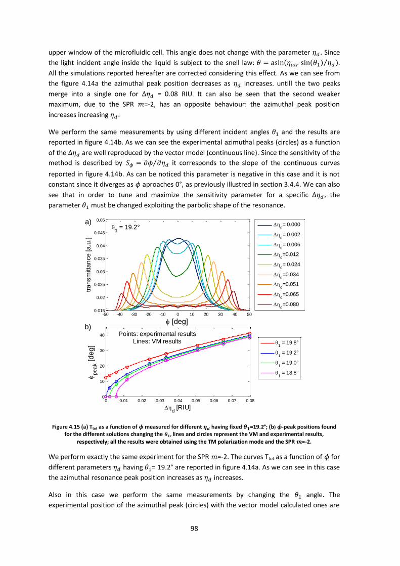
98
upper window of the microfluidic cell. This angle does not change with the parameter 𝜂𝑑 . Since
the light incident angle inside the liquid is subject to the snell law: 𝜃 = asin(𝜂𝑎𝑖𝑟 sin(𝜃1) 𝜂𝑑⁄ ).
All the simulations reported hereafter are corrected considering this effect. As we can see from
the figure 4.14a the azimuthal peak position decreases as 𝜂𝑑 increases. untill the two peaks
merge into a single one for Δ𝜂𝑑 = 0.08 RIU. It can also be seen that the second weaker
maximum, due to the SPR 𝑚=-2, has an opposite behaviour: the azimuthal peak position
increases increasing 𝜂𝑑 .
We perform the same measurements by using different incident angles 𝜃1 and the results are
reported in figure 4.14b. As we can see the experimental azimuthal peaks (circles) as a function
of the Δ𝜂𝑑 are well reproduced by the vector model (continuous line). Since the sensitivity of the
method is described by 𝑆𝜙 = 𝜕𝜙 𝜕𝜂𝑑⁄ it corresponds to the slope of the continuous curves
reported in figure 4.14b. As can be noticed this parameter is negative in this case and it is not
constant since it diverges as 𝜙 aproaches 0°, as previously illustred in section 3.4.4. We can also
see that in order to tune and maximize the sensitivity parameter for a specific Δ𝜂𝑑 , the
parameter 𝜃1 must be changed exploiting the parbolic shape of the resonance.
Figure 4.15 (a) Ttot as a function of 𝝓 measured for different 𝜼𝒅 having fixed 𝜽𝟏=19.2°; (b) 𝝓-peak positions found for the different solutions changing the 𝜽𝟏, lines and circles represent the VM and experimental results,
respectively; all the results were obtained using the TM polarization mode and the SPR 𝒎=-2.
We perform exactly the same experiment for the SPR 𝑚=-2. The curves Ttot as a function of 𝜙 for
different parameters 𝜂𝑑 having 𝜃1= 19.2° are reported in figure 4.14a. As we can see in this case
the azimuthal resonance peak position increases as 𝜂𝑑 increases.
Also in this case we perform the same measurements by changing the 𝜃1 angle. The
experimental position of the azimuthal peak (circles) with the vector model calculated ones are
-50 -40 -30 -20 -10 0 10 20 30 40 500.015
0.02
0.025
0.03
0.035
0.04
0.045
0.05
[deg]
tra
nsm
itta
nce
[a
.u.]
1 = 19.2°
d= 0.000
d= 0.002
d= 0.006
d=0.012
d= 0.024
d=0.034
d=0.051
d=0.065
d=0.080
0 0.01 0.02 0.03 0.04 0.05 0.06 0.07 0.080
10
20
30
40
d [RIU]
p
ea
k [deg]
Points: experimental resultsLines: VM results
1 = 19.8°
1 = 19.2°
1 = 19.0°
1 = 18.8°
a)
b)

99
reported in figure 4.14b. Also in this case 𝑆𝜙 is always positive and again it diverges as 𝜙
approaches 0°. Also in this case its values can be set just by changing the 𝜃1 angle.
Now we will analyse the sensitivity reached by this method and its Figure of Merit (FOM). We
will define three different FOMs and we will discuss which one best describe the resonance
proprieties. We will always compare our experimental results with the simulated behaviour.
Figure 4.16 |𝑺𝝓| plotted as a function of 𝝓𝒑𝒆𝒂𝒌. The marker represent the experimental points meanwhile the
shades areas represent the interval values calculated from the simulation using different incident angles. Blue
refers to the SPR 𝒎=1 and red to the SPR 𝒎=-2
In figure 4.16 we report |𝑆𝜙| as a function of the 𝜙 angle. We perform this analysis since we
noticed from figure 4.14b and 4.15b that if an azimuthal angle is taken into consideration the
slope of the curves 𝜙𝑝𝑒𝑎𝑘(𝜂𝑑) is almost the same regardless of the 𝜃1 used. In fact the curves
𝜙𝑝𝑒𝑎𝑘(𝜂𝑑) are almost parallel since them cannot intersect each other. The markers represent
the sensitivity values calculated by using the experimental results. The shaded areas represent
the interval values of sensitivity as a function of 𝜙𝑝𝑒𝑎𝑘 , we calculated by using the RCWA
method for different 𝜃1 angles. The different 𝜃1 were obtained by solving the equations 4.1 for
different values of 𝜂𝑑 . For the SPR 𝑚=1, 𝜃1 ranges from 33° to 40° while for SPR 𝑚=-2 it goes
from 14° to 19°. The blue colour refers to the SPR 𝑚=1 while the red one to the SPR 𝑚=-2. In the
RCWA method the parameter 𝜂𝑑 was varied in step of 0.0005 RIU in order to accurately retrieve
the sensitivity parameters.
As we can see the simulated curves do not have a huge dependence on 𝜃1 since the shaded area
are well confined in the plot. Nevertheless the sensitivity values of the SPR 𝑚=-2 appear more
affected by the 𝜃1 variations respect to the SPR 𝑚=1 since the red shaded area is wider than the
blue one. If an initial 𝜙𝑝𝑒𝑎𝑘=10° is set 𝑆𝜙 for the SPR 𝑚=-2 lays between 1000 deg/RIU and 1500
deg/RIU meanwhile for the SPR 𝑚=1 it is almost fixed to -1100 deg/RIU. This is due to the fact
that the parabolic shape factor 𝐾 introduced in eq. 3.8 varies quickly for the SPR 𝑚=-2 since for
low values of 𝜃1 the vertex 𝜃𝑐 of the resonance parabola shifts to lower incident angles with the
𝐾 parameter increasing.

100
The experimental sensitivity well agrees with the simulated one and in both cases it diverges
approaching 𝜙=0°. Hence, if we want to measure with an high sensitivity we need to have set an
initial azimuthal resonance having 𝜙𝑝𝑒𝑎𝑘 < 7°. We also notice that the maximum experimental
measured sensitivity reaches 3280 deg/RIU and 2280 deg/RIU for the SPR 𝑚=1 and 𝑚=-2,
respectively. If the initial resonance angle is set to 𝜙𝑝𝑒𝑎𝑘 > 20° the sensitivity has a value of 320
deg/RIU which slowly decreases with the increasing of 𝜙𝑝𝑒𝑎𝑘 . Even if the sensitivity diverges at
𝜙𝑝𝑒𝑎𝑘=0° it is very difficult to set the resonance at this azimuthal angle since the amplitude of
the peaks is very low and their position is strongly affected by small changes in 𝜃1.
In order to analyse the figure of merit of this azimuthal method, we define three different FOMs
as follows:
𝐹𝑂𝑀0 =|𝑆𝜙|
𝐹𝑊𝑀𝐻0; 𝐹𝑂𝑀𝑏 =
|𝑆𝜙|
𝐹𝑊𝑀𝐻𝑏; 𝐹𝑂𝑀𝑇 =
|𝑆𝜙|Δ𝑇
𝐹𝑊𝑀𝐻0 (4.2)
where 𝑆𝜙 is the azimuthal sensitivity, Δ𝑇 is the difference between the azimuthal peak
transmittance and the transmittance at 𝜙=0°. 𝐹𝑊𝑀𝐻0 is calculated considering the
transmittance at 𝜙=0° as the peak baseline while 𝐹𝑊𝑀𝐻𝑏 is calculated by using the
transmittance at 𝜙=90° as the peak baseline.
Figure 4.17 Schematic of the parameters used to calculate the FOMs and the two main cases that can appear.
Figure 4.17 shows a schematic of the two main cases that can appear and how we calculated the
FWMH. In the first case, the blue one, the two azimuthal peaks are well split and the 𝐹𝑊𝑀𝐻0 is
slightly lower than the 𝐹𝑊𝑀𝐻𝑏 since the transmittance at 𝜙 = 0° is slightly higher than the one
at 𝜙=90°. In the second case, the black one, the resonance peaks approach to 𝜙=0°. In this case
the 𝐹𝑊𝑀𝐻0 is smaller than the 𝐹𝑊𝑀𝐻𝑏 since the first one is related to the local azimuthal
peak shape and not to the total shape of the resonance curve, as it happens for 𝐹𝑊𝑀𝐻𝑏.
In figure 4.18a, 4.18b, and 4.18c we reported the values calculated for 𝐹𝑂𝑀0, 𝐹𝑂𝑀𝑏, and 𝐹𝑂𝑀𝑇
as a function of 𝜙𝑝𝑒𝑎𝑘. The points represent the values calculated from the experimental results,
while the shaded areas report the simulated results changing the incident angle 𝜃1 as previously
illustrated for the sensitivity case. The blue and red colours refer to the SPR 𝑚=1 and 𝑚=-2,
respectively.
In these cases the shaded areas are confined, hence the simulated FOMs as a function of 𝜙𝑝𝑒𝑎𝑘
do not depend on the 𝜃1 angle. Moreover the experimental behaviour is well reproduced by the
simulations. 𝐹𝑂𝑀0 starts from a values of 40 RIU-1 and grows up to 680 RIU-1 as 𝜙 approaches
-80 -60 -40 -20 0 20 40 60 800.01
0.02
0.03
0.04
0.05
0.06
0.07
0.08
[deg]
tra
nsm
itta
nce
[a
.u.]
FWMHb
TFWMH
0
FWMH0
FWMHb
T

101
0°. This parameter diverges as 𝜙𝑝𝑒𝑎𝑘 approaches 0° for two reasons. The first one is that |𝑆𝜙|
diverges and the second one is that the 𝐹𝑊𝑀𝐻0, for its definition, tends to 0° as
𝜙𝑝𝑒𝑎𝑘approaches 0°. Since it is at the denominator of 𝐹𝑂𝑀0 it contributes to its divergence.
The 𝐹𝑂𝑀𝑏 parameter starts from 35 RIU-1 and grows up to 90 RIU-1 as 𝜙𝑝𝑒𝑎𝑘 approaches 0°. We
can see that these values are lower than 𝐹𝑂𝑀0 and this is due to the fact that for definition
𝐹𝑊𝑀𝐻0 < 𝐹𝑊𝑀𝐻𝑏. The biggest difference between these two parameters is found at 𝜙𝑝𝑒𝑎𝑘
approaching 0° since the 𝐹𝑊𝑀𝐻0 tends to 0° while 𝐹𝑊𝑀𝐻𝑏 reaches an almost constant values
of 30°. Still this parameter diverges for 𝜙=0° because |𝑆𝜙| diverges. We can also notice some
discontinuities of the curves around 𝜙=15°~20°. These are due to the fact that here the peaks
merge and we effectively jump from a situation described by the blue curve, to a situation
described by the black curve of figure 4.17. This implies a discontinuous decreases in the
𝐹𝑊𝑀𝐻𝑏 even though this discontinuity has not an important physical meaning.
Figure 4.18 (a) 𝑭𝑶𝑴𝟎, (b) 𝑭𝑶𝑴𝒃, (c) 𝑭𝑶𝑴𝑻, plotted as a function of 𝝓𝒑𝒆𝒂𝒌. The marker represent the experimental
points meanwhile the shades areas represent the interval values calculated from the simulation using different
incident angles. Blue refers to the SPR 𝒎=1 and red to the SPR 𝒎=-2
The most interesting parameter 𝐹𝑂𝑀𝑇 is reported in figure 4.18c. It is calculated by multiplying
the 𝐹𝑂𝑀0 with Δ𝑇. This parameter tends to 0 a.u./RIU as 𝜙𝑝𝑒𝑎𝑘 approaches 0° and it removes
the divergence caused from both the parameter |𝑆𝜙| and 𝐹𝑊𝑀𝐻0. In detail 𝐹𝑂𝑀𝑇=0 a.u./RIU

102
when 𝜙𝑝𝑒𝑎𝑘 = 0° and then it increases reaching a maximum at 𝜙𝑝𝑒𝑎𝑘=20° for both the plasmonic
orders. After this maximum it slowly decreases as 𝜙𝑝𝑒𝑎𝑘 increases. This parameter is the one
that correctly describes the azimuthal behaviour of the plasmonic resonance. This is due to the
fact that the parameter Δ𝑇 takes into account how challenging is the SPR detection when 𝜙𝑝𝑒𝑎𝑘
approaches 0°. The 𝐹𝑂𝑀𝑇 parameter for the SPR 𝑚=1 (~1.7 a.u./RIU at its maximum) is higher
than the one for the SPR 𝑚=-2 (~0.7 a.u./RIU at its maximum) since the first resonance is better
than the second one. The experimental behaviour is well reproduced by the simulated data even
if for the SPR 𝑚=1 a shift to lower angles of the maximum seems to appear.
From this analysis we can conclude that if a peak starting position is chosen in the
10°<𝜙𝑝𝑒𝑎𝑘<20° interval |𝑆𝜙| is higher than 500 deg /RIU and the parameter 𝐹𝑂𝑀𝑇 has already
reached at least the 50 % of its maximum value. Obviously the SPR order has to be chosen on
the base of the experimental needs e.g. if the functionalization process is expected to increase
(decrease) the SPR coupling momentum then 𝑚=1 (𝑚=-2) must be prefer since in this case the
azimuthal angle resonance shifts to lower values, increasing in this way the method sensitivity.
We suspect that 𝐹𝑂𝑀𝑇 is the most correct parameter to apply in the study of the plasmonic
resonance sensitivity when it is enhanced by exploiting a parabolic shape resonance.
Nevertheless more studies need to be done in order to confirm this.
The resolution of this method depends on the accuracy of the bench azimuthal angle
positioning. In our case, it is related to the motorized rotation stage, being 0.01°. Considering
this value, we obtain a minimum resolution of 5 × 10⁻⁶ RIU, which is only fifty times larger than
the lowest reported resolution, i.e., 10-7 RIU [25].

103
4.4 Detection of Alkanethiols Self Assembled Monolayers
In this section we will see how the same azimuthal method, applied for sensing different 𝜂𝑑
values, can be adopted for sensing different Self Assembly Monolayer (SAM) adsorbed onto the
metallic grating surface. These SAMs are dielectric layers with the same refractive index 𝜂𝑑=1.45
but with a different thickness. By using them we will evaluate the sensitivity of the azimuthal
method respect to ℎ𝑓𝑢𝑛𝑐. We will measure this sensitivity considering both air and water as the
dielectric medium. In air we will sense the azimuthal shift produced by SAM created by different
alkanethiols molecules. In water we will monitor the adsorption onto the grating surface of the
6-mercapto-1-hexanol molecules taking advantage of our microfluidic setup.
4.4.1 Functionalization protocols
To create different type of SAM onto the grating surface we used five different types of
molecules. For the air sensitivity test we used alkanethiols molecules with different number of
methylene groups in their chain. These molecules are known in literature to form SAM with
different thickness [20], [82], [91], [101].This affect the SPP coupling constant since the thicker is
the SAM the greater is the SPP coupling momentum.
In particular we dipped five different grating samples into 1 mM ethanol solution of exanethiols
(C6), octanethiols (C8), dodecanethiols (C12), and octadecanethiols (C18). The chemical formula
of these molecule is CN = CH3(CH2)N-1SH, where N is the number of carbon atoms in their chain.
The thiol group S-H, known as head of the molecule, is the one that allows the link with the
metal layer losing its hydrogen atom and becoming an S-Ag group. The CH3 is the methyl
terminal group which is the one in contact with the buffer medium; (CH2)N-1 are the methylene
groups contained in the chain as schematically reported in figure 4.19.
Figure 4.19 Schematic of a SAM [102]
In order to test the sensibility in water we use another molecule: the 6-mercapto-1-hexanol or
MCH. Its chemical formulae is SH(CH2)5CH2OH. Again its head is a thiol and the tail is a primary
alcohol group. In order to functionalize the surface we used the MCH diluted in10 mM solution
of milli-q water.
We will refer to the surface without functionalization as bare condition.
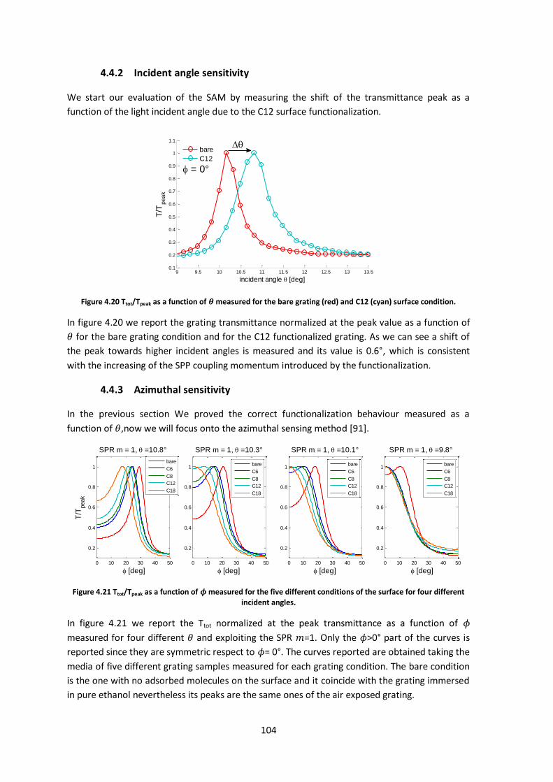
104
4.4.2 Incident angle sensitivity
We start our evaluation of the SAM by measuring the shift of the transmittance peak as a
function of the light incident angle due to the C12 surface functionalization.
Figure 4.20 Ttot/Tpeak as a function of 𝜽 measured for the bare grating (red) and C12 (cyan) surface condition.
In figure 4.20 we report the grating transmittance normalized at the peak value as a function of
𝜃 for the bare grating condition and for the C12 functionalized grating. As we can see a shift of
the peak towards higher incident angles is measured and its value is 0.6°, which is consistent
with the increasing of the SPP coupling momentum introduced by the functionalization.
4.4.3 Azimuthal sensitivity
In the previous section We proved the correct functionalization behaviour measured as a
function of 𝜃,now we will focus onto the azimuthal sensing method [91].
Figure 4.21 Ttot/Tpeak as a function of 𝝓 measured for the five different conditions of the surface for four different
incident angles.
In figure 4.21 we report the Ttot normalized at the peak transmittance as a function of 𝜙
measured for four different 𝜃 and exploiting the SPR 𝑚=1. Only the 𝜙>0° part of the curves is
reported since they are symmetric respect to 𝜙= 0°. The curves reported are obtained taking the
media of five different grating samples measured for each grating condition. The bare condition
is the one with no adsorbed molecules on the surface and it coincide with the grating immersed
in pure ethanol nevertheless its peaks are the same ones of the air exposed grating.
9 9.5 10 10.5 11 11.5 12 12.5 13 13.50.1
0.2
0.3
0.4
0.5
0.6
0.7
0.8
0.9
1
1.1
incident angle [deg]
T/T
pe
ak
bare
C12
= 0°
0 10 20 30 40 50
0.2
0.4
0.6
0.8
1
SPR m = 1, =10.8°
T/T
peak
[deg]
bare
C6
C8
C12
C18
0 10 20 30 40 50
0.2
0.4
0.6
0.8
1
[deg]
SPR m = 1, =10.3°
bare
C6
C8
C12
C18
0 10 20 30 40 50
0.2
0.4
0.6
0.8
1
[deg]
SPR m = 1, =10.1°
bare
C6
C8
C12
C18
0 10 20 30 40 50
0.2
0.4
0.6
0.8
1
[deg]
SPR m = 1, =9.8°
bare
C6
C8
C12
C18

105
As we already seen for glycerol/water solution case, the incident angle allows us to change the
azimuthal shift between the different conditions. As we can see, for 𝜃= 10.8° an azimuthal peak
𝜙 ≠ 0° can be detected for all the five different conditions, while, for 𝜃= 10.3°, only an
azimuthal peak at 𝜙=0° can be seen for the C18 condition. Taking this particular case the shift
between the C12 condition and the C18 goes from 3.88° for 𝜃= 10.8° to 7.55° for 𝜃 = 10.3°
doubling its value. Similar considerations can be performed for 𝜃= 10.1° where the C12 condition
produces a single peak, and for 𝜃= 9.8° where the C8 and C6 azimuthal peaks are merged at
𝜙=0°.
The azimuthal peak position for the four different incident angles and for all the five conditions
measured are reported in figure 4.23a. It is obvious that when two functionalization conditions
have one single peak at 𝜙=0° it is impossible to distinguish them by this azimuthal method.
We perform the same experiment taking into consideration the 𝑚=-2 SPR condition.
Figure 4.22 Ttot/Tpeak as a function of 𝝓 measured for the five different conditions of the surface for four different incident angles.
In figure 4.22 we report the Ttot normalized at the peak transmittance as a function of 𝜙
measured for four different 𝜃 and for the 𝑚=-2 SPR. Only the 𝜙>0° part of the curves is reported
since they are symmetry respect to 𝜙= 0°.
Also in this case the figure 4.22 well shows how different 𝜃 affects the shift between the
conditions. For 𝜃=46.5° all the surface conditions have an azimuthal peak 𝜙 > 0°, meanwhile for
𝜃 = 43.7° the bare conditions shows a peak slightly above 𝜙=0°. In this case the shift between
the C6 and bare condition is amplified from 0.98° to 3.99° by using the bare optimized incident
angle. Decreasing again the incident angle also the C6 and the C12 conditions has only a
maximum at 𝜙 = 0°. The azimuthal peak position and the incident angle for all the five conditions
measured are reported in figure 4.23b.
0 5 10 15 200.2
0.3
0.4
0.5
0.6
0.7
0.8
0.9
1
1.1
T/T
peak
[deg]
SPR m = -2, =46.5°
bare
C6
C8
C12
C18
0 5 10 15 200.2
0.3
0.4
0.5
0.6
0.7
0.8
0.9
1
1.1
[deg]
SPR m = -2, = 43.7°
bare
C6
C8
C12
C18
0 5 10 15 200.2
0.3
0.4
0.5
0.6
0.7
0.8
0.9
1
1.1
[deg]
SPR m = -2, = 43.2°
bare
C6
C8
C12
C18
0 5 10 15 200.2
0.3
0.4
0.5
0.6
0.7
0.8
0.9
1
1.1
[deg]
SPR m = -2, = 42.9°
bare
C6
C8
C12
C18

106
Figure 4.23 Comparison between experimental data (points with error bars) and Vector Model simulations (solid lines) for the peak azimuthal angles as a function of the refractive effective index variation. Values of 𝜟𝜼𝒆𝒇𝒇 =(0,
4.9,5.8,8.2,11.4)×10-3 correspond to the different surface grating conditions. (a) SPR order 𝒎=1; (b)SPR 𝒎=-2.
In Figure 4.23a and 4.23b we show the azimuthal angle position of the SPR, for various incident
angles, as a function of the effective refractive index variations 𝛥𝜂𝑒𝑓𝑓 for 𝑚 = 1 and 𝑚 = −2,
respectively. The continuous lines correspond to the VM simulation results, while the
experimental points are reported with their error bars for each grating condition. The parameter
𝛥𝜂𝑒𝑓𝑓 only affects the SPP coupling constant modifying eq. 1.24 into:
𝑘𝑠𝑝𝑝 = 𝑘0√(1+ 𝛥𝜂𝑒𝑓𝑓)
2휀𝑚
(1 + 𝛥𝜂𝑒𝑓𝑓)2+ 휀𝑚
(4.3)
𝛥𝜂𝑒𝑓𝑓 takes into account the modifications introduced by the surface functionalization on the
SPR behaviour. Hence the different surface conditions are represented in the x−axis by the
different values of 𝛥𝜂𝑒𝑓𝑓 . For reference, 𝛥𝜂𝑒𝑓𝑓 is set to 0 RIU for the bare grating, while it was
calculated for the other conditions by using the effective medium approximation model as
previously illustrated in eq. 3.5 and in the following one.
𝜂𝑒𝑓𝑓 = 𝜂𝑑 +2ℎ𝑓𝑢𝑛𝑐𝑑𝑧
(𝜂𝑓𝑢𝑛𝑐 − 𝜂𝑑) (4.4)
To perform the calculations we used 0.6 nm, 0.9 nm, 1.5 nm, and 2.2 nm as the thickness values
ℎ𝑓𝑢𝑛𝑐 for the four different SAMs and 𝜂𝑓𝑢𝑛𝑐=1.45 RIU; these values are similar to the one
reported in [82]. For the plasmon penetration length 𝑑𝑧 we used 160 nm. It is evident that the
sensitivity parameter is defined in this case as 𝑆𝜙 = 𝜕𝜙/𝜕𝜂𝑒𝑓𝑓 and corresponds to the slope of
these curves. Its experimental values as a function of 𝜃 are shown in table 4.3. Considering now
figure 4.23a for 𝑚 = 1, we see that the curves slope is always negative and tends to diverge as ϕ
approaches 0°. In the same way we can notice that the sensitivity for 𝑚 = −2 is always positive
and diverges for ϕ = 0° as already seen for the measurements performed by using the
glycerol/water solutions.
0 2 4 6 8 10 12
x 10-3
0
5
10
15
20
25
30
eff 10-3 [RIU]
azim
uta
l a
ng
le [d
eg
]
= 10.8°
= 10.3°
= 10.1°
= 9.8°
14
16
= 46.5°
0 2 4 6 8 10 12
x 10-3
0
2
4
6
8
10
eff 10-3 [RIU]
= 43.7°
= 43.2°
= 42.9°
a) b)
SPR m = -2SPR m = 1

107
SPR 𝑚 = 1 SPR 𝑚 = -2
𝜃 [𝑑𝑒𝑔] 𝑆𝜙 [𝑑𝑒𝑔]/[𝑅𝐼𝑈]; C6-Bare 𝜃 [𝑑𝑒𝑔] 𝑆𝜙 [𝑑𝑒𝑔]/[𝑅𝐼𝑈]; C18-C12
10.8 -930 46.5 180
10.3 -1220 43.7 390
10.1 -1570 43.2 460
9.8 -2180 42.9 1180 Table 4.3 Sensitivity measured at different incident angles.
In table 4.3 we report the experimental sensitivity values calculated by using the surface
condition pairs that allow the sensitivity evaluation for each incident angle tested. These pairs
correspond to the C6 and the bare condition for 𝑚 = 1, and to the C18 and the C12 conditions
for 𝑚 = −2. A clear sensitivity enhancement of a factor 2.4 is reached for 𝑚 = 1, while it grows up
to 6.5 for 𝑚 = −2 SPR. The sensitivity reaches values up to 2180 deg/RIU, and 1180 deg/RIU in
the two cases, being twenty times higher than the 80 deg/RIU evaluated using the incident angle
shift reported in figure 4.20, which is a noticeable improvement.
Regarding the sensitivity in water we measured the kinetic adsorption of the MCH molecules onto the silver metal layer.
Figure 4.24 (a) Azimuthal peak as a function of the time. (b) Vector model simulation for the two measured surface.
(c) Azimuthal angle variations ∆𝝓 as a function of the initial peak condition 𝝓𝒃𝒂𝒓𝒆
In figure 4.24a we report the azimuthal peak as a function of the time. For the first 20 minutes
we fluxed milli-q water inside the microfluidic cell. Then we changed the solution with the 10
mM MCH one and we waited 15 minutes, then we fluxed again milli-q water. All the process
were performed having a fixed flux of 50 μL/min. After the introduction of the MCH solution the
azimuthal peak position dropped. This is due to the fact that the molecules present in the
solutions have quickly formed a SAM on the silver surface. When we inserted again the milli-q
water the 𝜙 angle did not change again confirming that the decrease of the resonance azimuthal
5 10 15 20 25 30 35 40 45 500
5
10
15
20
25
30
35
time [min]
[deg]
MCH 10 mM
23.8 24 24.2 24.4 24.6 24.8 250
5
10
15
20
25
[deg]
[deg]
Vector Model Simulations
bare eff
= 0
MCH eff
= 2.310-3
0 5 10 15 20 25 30 35 40-8
-6
-4
-2
0
bare
[deg]
=
m
ch -
bare
[d
eg
]
experimental
vector model
b)
c)
a)
Milli-q Milli-q

108
position was due to the SAM formation rather than a change of the MCH refractive index
solution.
In figure 4.19b we report the two azimuthal resonances one for the bare grating condition and
one for the MCH grating condition calculated by using a 𝛥𝜂𝑒𝑓𝑓= 2.3 x 10⁻³ RIU. In figure 4.19c we
report the 𝛥𝜙 = 𝜙𝑀𝐶𝐻 − 𝜙𝐵𝑎𝑟𝑒 plotted as a function of the 𝜙𝐵𝑎𝑟𝑒 condition. The red circles
refers to the experimental values and can be calculated by measuring the height of the
azimuthal steps reported in figure 4.19a while the continuous line refer to the VM calculations
that can be retrieved by the curves reported in figure 4.19b.
Also in this case we can see a good agreement between the experimental points and the vector
model predicted behaviour. As usual we also notice that 𝛥𝜙 increases as 𝜙𝐵𝑎𝑟𝑒 approaches to
6°. For 𝜙𝐵𝑎𝑟𝑒 <6° the parameter 𝛥𝜙 decreases because the functionalization condition always
produces a peak at 𝜙=0°.

109
4.5 Detection of an antibody layer
In the previous section we illustrated how to implement an azimuthal sensing method to
evaluate both the change in the buffer refractive index (𝜂𝑑) and in the SAM formation. Here we
want to apply this method to detect the surface variations induced by two subsequent
functionalization processes. The first one will produce a cross link SAM by using a
carboxymethyl-polyethylene glycol-thiol (PEG). This SAM will exposed a carboxylic group that
will be modified in order to immobilized an antibody layer exploiting the ammine groups
available on the antibody surface. We will study how the concentration of the PEG and the
presence of the antibody will affect the resonance both in the Kretschmann and grating
configurations.
4.5.1 Functionalization protocols
In order to perform this experiment we used a drop casting method. The drops (30 μL) were
applied on our device by means of a socket (Grace Bio-Labs ProPlate® microarray system, 64).
The carboxymethyl-PEG-Thiol with a molecular weight of 3400 Dalton were purchased by
(laysanBio). We used N-(3-Dimethylaminopropyl)-N′-ethylcarbodiimide (EDC) and sulfo-N-
Hydroxysuccinimide (s-NHS) in MES buffer (sigma Aldrich) in order to activate the carboxylic
group of the PEG and link it to an ammine group of the antibody anti (E. Coli) (Virostat).
For the antibodies immobilization, the surface was immersed in a 1 mM PEG/milli-q solution
overnight and then rinsed with milli-qwater and dried under nitrogen flux. The PEG carboxylic
group was activated through EDC and sulfo-NHS 5 mM each in MES buffer pH 6 for 15 minutes
(MES buffer: 0.1M 2-(N-morpholino) ethanesulfonic acid (MES), 0.5M NaCl).After the activation
the surface were again rinsed with milli-q water and dried under nitrogen flux.
The anti E. coli antibody at the concentration of 1 mg/mL is then applied to the surface through
a printing buffer: Na2PO4 0.1 M, NaCl 0.3 M, Triton X-100 0,01%, pH 7.2. Then surface, with the
immobilized antibodies, is rinsed in milli-q water and dried in air.
We functionalized our devices as reported in these schemes of table 4.4:
PEG study Antibody study
Orange spot PEG 1 mM Yellow spot PEG 0.1 mM or 0.5 mM Cyan spot milli-q
Orange spotPEG 1 mM Yellow spot PEG + Ab Cyan spot milli-q
Table 4.4 schematic of the functionalization protocols.
Our standard device is a rectangular array of spots, where only the internal ones were used. For
the measurements in Kretschmann configuration we will used a flat surface while for the one in
grating configuration we will used the nanostructured surface. We will report different test
referring to different devices. For each test the experimental points report the average value of
the plasmonic resonance position performed over all the same coloured spots.

110
4.5.2 Incident angle sensitivity (Kretschmann configuration)
We will start by analysing the signals we obtained in the Kretschmann configuration.
Figure 4.25 (a) Angular shift of the plasmonic resonance respect to the milli-q plotted as a function of the PEG concentration. (b) R0 as function of the motor angle for the different PEG concentrations
In Figure 4.25a we report the average shift of the SPR from the milli-q condition as a function of
the Peg concentrations. In figure 4.25b we report the parameter R0 as a function of the
motorized angle obtained in the first test. As we can notice from figure 4.25a an angular shift up
to 1.1° for the SPR minimum position is obtained increasing the PEG concentration. Nevertheless
we can also noticed that a huge difference of 0.5° is found between the two test regarding the
same 1mM concentrations. In figure 4.25b we can also see how the plasmonic response is
affected by the PEG functionalization. Besides the shift of the resonance minimum we notice a
slight enhancement of its value. Unfortunately, we cannot increase the PEG concentration to 10
mM because this will damage the silver metal layer. Since we want to create a SAM over the
silver layer a 1 mM PEG/milli-q solution will be used in the antibodies immobilization test.
Figure 4.26 (a) Angular shift of the plasmonic resonance respect to the milli-q plotted as a function of the surface
condition. (b) R0 as function of the motor angle for the different surface conditions.
In Figure 4.26a we reported the results obtained for four different functionalization tests. The y-
axis reports the shift from the SPR position in the milli-q spot respect to the SPR position
measured for the other two surface cases i.e. surface with PEG and antibodies (Δ𝜃 = 𝜃𝑓𝑢𝑛𝑐 −
𝜃𝑚𝑖𝑙𝑙𝑖−𝑞); meanwhile the x-axis label represents the spot condition. As we can see always the

111
1mM PEG induced a shift between 0.6° and 1.1° as previously noticed; but not always the
antibodies seem to bind with the PEG i.e. the shift between PEG and PEG+antibodies is 0.4° for
the first and second tests, while it is almost undetectable for the third and fourth test. In figure
4.22b we report the parameter R0 as a function of the motorized angle, for the three different
surface conditions measured in the second test.
The antibodies sometimes do not produce the expected resonance shift. This behaviour suggests
that the antibodies immobilization protocol we used needs to be tuned in order to ensure the
results reliability. Another uncertainty factor is the use of silver as metal, in fact it is more
instable than gold which is the standard in this type of application.
4.5.3 Azimuthal angle sensitivity
The same experimental test were performed by using the grating configuration.
Figure 4.27(a) Angular shift of the plasmonic resonance respect to the milli-q plotted as a function of the
concentration. (b) Ttot/Tpeak as function of 𝝓 for the different PEG concentrations
In Figure 4.27a we report the average position of the azimuthal SPR respect to the milli-q
condition as a function of the PEG concentrations. In figure 4.27b we report the parameter Ttot
normalized at the peak transmittance as a function of the azimuthal angle for the different PEG
concentrations, as obtained in the first test. A noticeable shift of the transmittance maximum is
registered as a function of the PEG concentration. As we can notice from figure 4.27a, an angular
shift up to 5° of the SPR maximum position is obtained increasing the PEG concentration. Since
the metal layer we used is silver, it is not possible to further increase the PEG concentration up
to 10 mM; for this reason in the next test we will used the 1mM PEG/milli-q solution in order to
form the initial SAM.
In Figure 4.28a we report the results obtained for four different functionalization tests. As in the
previous case, the y-axis reports the difference between the average functionalized SPR position
and the milli-q, meanwhile the x-axis labels represent the condition of the spot. As we can see
the 1mM PEG induced a shift between 3.5° and 5°. Also in this case, not always the antibodies
seem to bind with the PEG layer as we can see for the test 3. The shifts between PEG and
PEG+antibody reaches 3° for the second test while it is almost 1° for the first and fourth test.
Regarding the third test we cannot detect a clear shift induced by the antibodies. In figure 4.28b

112
we report the parameter R0 as a function of the azimuthal angle, for the three different grating
surface conditions measured in the second test.
Figure 4.28(a) Angular shift of the plasmonic resonance respect to the milli-q plotted as a function of the surface
condition. (b) R0 Ttot/Tpeak as a function of 𝝓 for the different surface conditions.
In the following table we summarized the shift obtained between the milli-q treated spots and
the ones with the PEG and antibodies both for the Kretschmann and the grating configuration.
Kretschmann ∆𝜃𝐾[deg] Grating ∆𝜙𝐺[deg] Ratio ∆𝜙𝐺/∆𝜃𝐾
|𝑆𝑃𝑅𝑃𝐸𝐺 − 𝑆𝑃𝑅𝑚𝑖𝑙𝑙𝑖−𝑞| 0.6 ÷ 1.1 3.5 ÷ 5 4.5 ÷ 5.8
|𝑆𝑃𝑅𝐴𝑏 − 𝑆𝑃𝑅𝑚𝑖𝑙𝑙𝑖−𝑞| 1 ÷ 1.5 5 ÷ 6.5 4.3 ÷ 5.0 Table 4.5 Comparison between the shift variations found in Kretschmann and Grating configuration and the ration
of their shift.
As we can see from table 4.5 the ratio of the shifts calculated by using the two configuration is
between 4.3 and 5.5. This is consistent with our simulation since the sensitivity of the
Kretschmann configuration is 54 deg/RIU (see table 3.8) while the sensitivity for the azimuthal
configuration having an initial peak at 48° is almost 240 deg/RIU (see figure 4.16). The ratio
between these two sensitivities is 4.4 which is in the range of the experimental one. Hence
similar functionalizations of the two surface types similarly affect the SPP coupling constant.
Moreover comparing the two different detection techniques i.e. the Kretschmann one and the
azimuthal one we retrieved almost the same information:
The shifts caused by the PEG functionalization always produces a SPR shift but its value
could be subject to huge variations: from 0.6° to 1.1° for the Kretschmann configuration
and from 3.5° to 5° for the grating configuration.
The antibody binding protocol needs to be tuned in order to improve the reliability of
the method since in some cases we have not detected any plasmonic resonance
variation.

113
5 Conclusions
In this work we showed how different excitation and detection methods of the Surface Plasmon
Resonance phenomenon can be exploited for general sensing purposes. We reached this goal by
using both simulations and experimental measurements.
Regarding the simulations, we implemented three different methods: the Rigorous Coupled
Wave Analysis, the Chandezon, and the Finite Element method. We compared their results and
briefly discussed their properties and applications. Nevertheless another simpler method was
analysed: the vector model. By using these tools we were able to compute the intensities of all
the light rays diffracted by a periodic, one or two dimensional, nanostructured surface. We also
showed how the vector model well reproduces the simulated resonances even if it did not
provide qualitative information about their shape.
Applying these simulations methods to the nanostructured surface in conical mounting
configuration we noticed that the plasmonic resonance has a fixed parabolic shape and hence
there are no great benefits in having a two dimensional periodic surface instead of a one
dimensional grating. The result we found adding a further periodicity dimension is that the
azimuthal position of the plasmonic vertex 𝜙𝑐 can be different from 0°. We have also shown how
the relative intensities of the resonances can be changed by adding some features inside the
periodic cell.
Through the simulation methods we analyzed what happens in the Kretschmann configuration
when a grating is considered. In this case two SPPs seem to be excited. The first one it is related
to the metal/air interface and its excitation does not depend on the grating itself since this
plasmon is excited exploiting the Kretschmann excitation scheme. The second one is related to
the SPP at the metal/polycarbonate interface and it is excited through the grating. This SPP is
not affected by the refractive index variation at the silver/air interface, hence it can be used as a
reference in a Kretschmann measurements. The presence of these two plasmonic resonances
were also experimentally confirmed.
Furthermore we depicted the link between Kretschmann and grating configuration. The rays
transmitted by the grating when it is lighted in conical mounting configuration did not carry the
same amount of information. We saw that only two rays are significant: the baseline ray and the
Kretschmann ray and we generalized this aspect for both the SPR 𝑚=1 and 𝑚=-2 orders.
The simulations were used also for the evaluation of the bulk sensitivity to the buffer refractive
index 𝜂𝑑 , and functionalization thickness ℎ𝑓𝑢𝑛𝑐 parameters. In particular we analyzed the
sensitivity considering as sensing parameters the wavelength, the incident angle, the
polarization angle and the azimuthal angle. We also showed that an almost parabolic shape of
the plasmonic resonance allows a sensitivity enhancement and we revealed the main common
features of this detection method taking the azimuthal case as example.
Experimentally we optimized two optical benches for the detection of the SPR. One for the
grating in conical mounting configuration and the other for the Kretschmann configuration. We
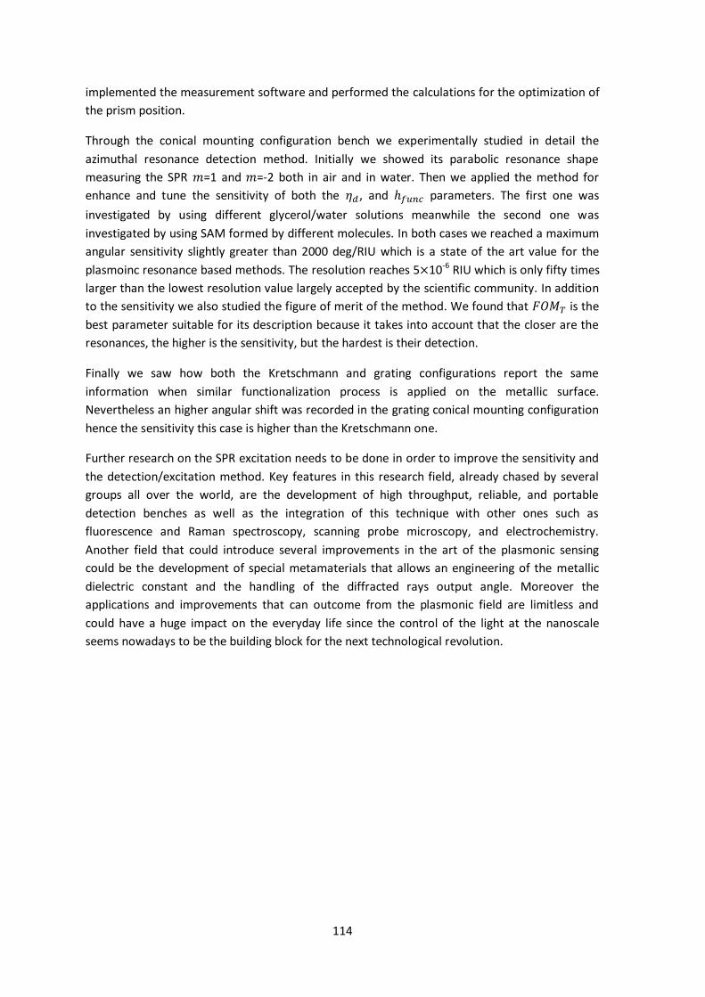
114
implemented the measurement software and performed the calculations for the optimization of
the prism position.
Through the conical mounting configuration bench we experimentally studied in detail the
azimuthal resonance detection method. Initially we showed its parabolic resonance shape
measuring the SPR 𝑚=1 and 𝑚=-2 both in air and in water. Then we applied the method for
enhance and tune the sensitivity of both the 𝜂𝑑 , and ℎ𝑓𝑢𝑛𝑐 parameters. The first one was
investigated by using different glycerol/water solutions meanwhile the second one was
investigated by using SAM formed by different molecules. In both cases we reached a maximum
angular sensitivity slightly greater than 2000 deg/RIU which is a state of the art value for the
plasmoinc resonance based methods. The resolution reaches 5×10⁻⁶ RIU which is only fifty times
larger than the lowest resolution value largely accepted by the scientific community. In addition
to the sensitivity we also studied the figure of merit of the method. We found that 𝐹𝑂𝑀𝑇 is the
best parameter suitable for its description because it takes into account that the closer are the
resonances, the higher is the sensitivity, but the hardest is their detection.
Finally we saw how both the Kretschmann and grating configurations report the same
information when similar functionalization process is applied on the metallic surface.
Nevertheless an higher angular shift was recorded in the grating conical mounting configuration
hence the sensitivity this case is higher than the Kretschmann one.
Further research on the SPR excitation needs to be done in order to improve the sensitivity and
the detection/excitation method. Key features in this research field, already chased by several
groups all over the world, are the development of high throughput, reliable, and portable
detection benches as well as the integration of this technique with other ones such as
fluorescence and Raman spectroscopy, scanning probe microscopy, and electrochemistry.
Another field that could introduce several improvements in the art of the plasmonic sensing
could be the development of special metamaterials that allows an engineering of the metallic
dielectric constant and the handling of the diffracted rays output angle. Moreover the
applications and improvements that can outcome from the plasmonic field are limitless and
could have a huge impact on the everyday life since the control of the light at the nanoscale
seems nowadays to be the building block for the next technological revolution.

115
6 Acknowledgements
I would like to thank everyone that helped me through this PhD experience, especially my
supervisor, Prof. Alessandro Paccagnella and my colleagues Alessandro De Toni, Elisabetta
Pasqualotto, Giulio Rosati, and Matteo Scaramuzza and the Master thesis students Alessandro
Zanuoli, Federico Carlesso and Silvia Guggia.
Moreover I acknowledge Prof. Nikolay Zheludev and Fedotov Vassili for the fruitful period I
spent with their group at the Optoelectronic Centre of the Southampton university. The Veneto
Nanotech group headed by Erica Cretaio for their precious contribution on the implementation
of the functionalization processes, the Luxor Laboratories headed by Maria Guglielmina Pelizzo
for the access to the Kretschmann configuration bench.
I cannot forget my parents and all my family for the support they gave me and also all my
friends, the old ones, from the mountains, and the new ones of the Padova Rugby 555.
And finally I would like to thank Alessandra for always share with me the beautiful and sad
moments.
Thank you all...

116

117
7 Bibliography
[1] R. W. Wood, “A suspected case of the Electrical Resonance of Minute Metal Particles for Light-waves. A New Type of Absorption,” Proc. Phys. Soc. London, vol. 18, no. 1, pp. 166–182, Mar. 1902.
[2] U. FANO, “The Theory of Anomalous Diffraction Gratings and of Quasi-Stationary Waves on Metallic Surfaces (Sommerfeld’s Waves),” J. Opt. Soc. Am., vol. 31, no. 3, p. 213, Mar. 1941.
[3] A. Otto, “Excitation of nonradiative surface plasma waves in silver by the method of frustrated total reflection,” Zeitschrift für Phys., vol. 216, no. 4, pp. 398–410, Aug. 1968.
[4] E. Kretschmann and H. Raether, “Radiative Decay of Non Radiative Surface Plasmons Excited by Light,” Zeitschrift für Naturforsch., vol. 23a, pp. 2135–2136, 1968.
[5] D. Hornauer, H. Kapitza, and H. Raether, “The dispersion relation of surface plasmons on rough surfaces,” J. Phys. D. Appl. Phys., vol. 7, no. 9, pp. L100–L102, Jun. 1974.
[6] J. G. Gordon and J. D. Swalen, “The effect of thin organic films on the surface plasma resonance on gold,” Opt. Commun., vol. 22, no. 3, pp. 374–376, Sep. 1977.
[7] B. Liedberg, C. Nylander, and I. Lunström, “Surface plasmon resonance for gas detection and biosensing,” Sensors and Actuators, vol. 4, pp. 299–304, 1983.
[8] B. Liedberg, C. Nylander, and I. Lundström, “Biosensing with surface plasmon resonance — how it all started,” Biosens. Bioelectron., vol. 10, no. 8, pp. i–ix, Jan. 1995.
[9] J. Homola, S. S. Yee, and G. Gauglitz, “Surface plasmon resonance sensors: review,” Sensors Actuators B Chem., vol. 54, no. 1–2, pp. 3–15, 1999.
[10] X. D. Hoa, a G. Kirk, and M. Tabrizian, “Towards integrated and sensitive surface plasmon resonance biosensors: a review of recent progress.,” Biosens. Bioelectron., vol. 23, no. 2, pp. 151–60, Sep. 2007.
[11] K. S. Phillips and Q. Cheng, “Recent advances in surface plasmon resonance based techniques for bioanalysis,” in Analytical and Bioanalytical Chemistry, 2007, vol. 387, pp. 1831–1840.
[12] J. Homola, “Surface plasmon resonance sensors for detection of chemical and biological species.,” Chem. Rev., vol. 108, no. 2, pp. 462–93, Feb. 2008.
[13] S. Scarano, M. Mascini, A. P. F. Turner, and M. Minunni, “Surface plasmon resonance imaging for affinity-based biosensors.,” Biosens. Bioelectron., vol. 25, pp. 957–966, 2010.
[14] I. Lundström, “From a Laboratory Exercise for Students to a Pioneering Biosensing Technology,” Plasmonics, vol. 1, no. 11, 2014.
[15] S. A. Maier, Plasmonics: Fundamentals and applications. 2007, pp. 1–223.

118
[16] J. Homola, Surface Plasmon Resonance Based Sensors. 2006.
[17] R. B. M. Schasfoort and A. J. Tudos, Handbook of surface plasmon resonance, vol. 240. 2008, p. xxi, 403 p.
[18] A. P. F. Turner, “Biosensors: sense and sensibility.,” Chem. Soc. Rev., vol. 42, pp. 3184–96, 2013.
[19] U. Jönsson, L. Fägerstam, B. Ivarsson, B. Johnsson, R. Karlsson, K. Lundh, S. Löfås, B. Persson, H. Roos, and I. Rönnberg, “Real-time biospecific interaction analysis using surface plasmon resonance and a sensor chip technology.,” Biotechniques, vol. 11, pp. 620–627, 1991.
[20] L. Jung, C. Campbell, and T. Chinowsky, “Quantitative interpretation of the response of surface plasmon resonance sensors to adsorbed films,” Langmuir, vol. 7463, no. 17, pp. 5636–5648, 1998.
[21] E. J. Zeman and G. C. Schatz, “An accurate electromagnetic theory study of surface enhancement factors for silver, gold, copper, lithium, sodium, aluminum, gallium, indium, zinc, and cadmium,” J. Phys. Chem., vol. 91, no. 3, pp. 634–643, Jan. 1987.
[22] B. D. Gupta and R. K. Verma, “Surface Plasmon Resonance-Based Fiber Optic Sensors: Principle, Probe Designs, and Some Applications,” J. Sensors, vol. 2009, pp. 1–12, 2009.
[23] Y. Fu and X. Zhou, “Plasmonic Lenses: A Review,” Plasmonics, vol. 5, no. 3, pp. 287–310, Jun. 2010.
[24] H. Kim, J. Park, S.-W. Cho, S.-Y. Lee, M. Kang, and B. Lee, “Synthesis and dynamic switching of surface plasmon vortices with plasmonic vortex lens.,” Nano Lett., vol. 10, no. 2, pp. 529–36, Feb. 2010.
[25] M. Piliarik and J. Homola, “Surface plasmon resonance (SPR) sensors: approaching their limits?,” Opt. Express, vol. 17, no. 19, pp. 16505–16517, 2009.
[26] N. J. Tao, S. Boussaad, W. L. Huang, R. a. Arechabaleta, and J. D’Agnese, “High resolution surface plasmon resonance spectroscopy,” Rev. Sci. Instrum., vol. 70, no. 12, p. 4656, 1999.
[27] R. Slavík and J. Homola, “Ultrahigh resolution long range surface plasmon-based sensor,” Sensors Actuators B Chem., vol. 123, no. 1, pp. 10–12, Apr. 2007.
[28] G. Ruffato and F. Romanato, “Grating-coupled surface plasmon resonance in conical mounting with polarization modulation,” Opt. Lett., vol. 37, no. 13, p. 2718, 2012.
[29] G. Granet and L. Li, “Convincingly converged results for highly conducting periodically perforated thin films with square symmetry,” J. Opt. A Pure Appl. Opt., vol. 8, no. 6, pp. 546–549, Jun. 2006.
[30] S. Y. Wu, H. P. Ho, W. C. Law, C. Lin, and S. K. Kong, “Highly sensitive differential phase-sensitive surface plasmon resonance biosensor based on the Mach-Zehnder configuration.,” Opt. Lett., vol. 29, pp. 2378–2380, 2004.

119
[31] H. Bai, R. Wang, B. Hargis, H. Lu, and Y. Li, “A SPR aptasensor for detection of avian influenza virus H5N1.,” Sensors (Basel)., vol. 12, no. 9, pp. 12506–18, Jan. 2012.
[32] R. L. Caygill, G. E. Blair, and P. a Millner, “A review on viral biosensors to detect human pathogens.,” Anal. Chim. Acta, vol. 681, no. 1–2, pp. 8–15, Nov. 2010.
[33] Z. Altintas, Y. Uludag, Y. Gurbuz, and I. E. Tothill, “Surface plasmon resonance based immunosensor for the detection of the cancer biomarker carcinoembryonic antigen.,” Talanta, vol. 86, pp. 377–83, Oct. 2011.
[34] Z. Altintas and I. Tothill, “Biomarkers and biosensors for the early diagnosis of lung cancer,” Sensors Actuators B Chem., vol. 188, pp. 988–998, Nov. 2013.
[35] J. Wei, Y. Mu, D. Song, X. Fang, X. Liu, L. Bu, H. Zhang, G. Zhang, J. Ding, W. Wang, Q. Jin, and G. Luo, “A novel sandwich immunosensing method for measuring cardiac troponin I in sera,” Anal. Biochem., vol. 321, no. 2, pp. 209–216, Oct. 2003.
[36] Y. Yanase, T. Hiragun, T. Yanase, T. Kawaguchi, K. Ishii, and M. Hide, “Application of SPR Imaging Sensors for detection of individua living cell reaction and clinical diagnosisof Type I allergy,” Allergol. Int., vol. 62, no. 2, pp. 163–9, Jun. 2013.
[37] K. Hegnerová, M. Bocková, H. Vaisocherová, Z. Krištofiková, J. Říčný, D. Řípová, and J. Homola, “Surface plasmon resonance biosensors for detection of Alzheimer disease biomarker,” Sensors Actuators B Chem., vol. 139, no. 1, pp. 69–73, May 2009.
[38] T. F. McGrath, J. Buijs, a. C. Huet, P. Delahaut, C. T. Elliott, and M. H. Mooney, “Assessment of a multiplexing high throughput immunochemical SPR biosensor in measuring multiple proteins on a single biosensor chip,” Sensors Actuators B Chem., vol. 186, pp. 423–430, Sep. 2013.
[39] E. Mauriz, a Calle, J. J. Manclús, a Montoya, and L. M. Lechuga, “Multi-analyte SPR immunoassays for environmental biosensing of pesticides.,” Anal. Bioanal. Chem., vol. 387, no. 4, pp. 1449–58, Feb. 2007.
[40] R. Yatabe, T. Onodera, and K. Toko, “Fabrication of an SPR sensor surface with antifouling properties for highly sensitive detection of 2,4,6-trinitrotoluene using surface-initiated atom transfer polymerization.,” Sensors (Basel)., vol. 13, no. 7, pp. 9294–304, Jan. 2013.
[41] H. Bao, T. Wei, X. Li, Z. Zhao, H. Cui, and P. Zhang, “Detection of TNT by a molecularly imprinted polymer film-based surface plasmon resonance sensor,” Chinese Sci. Bull., vol. 57, no. 17, pp. 2102–2105, Apr. 2012.
[42] S. Wang, E. S. Forzani, and N. Tao, “Detection of heavy metal ions in water by high-resolution surface plasmon resonance spectroscopy combined with anodic stripping voltammetry.,” Anal. Chem., vol. 79, no. 12, pp. 4427–32, Jun. 2007.
[43] J. D. Wright, J. V. Oliver, R. J. M. Nolte, S. J. Holder, N. a. J. M. Sommerdijk, and P. I. Nikitin, “The detection of phenols in water using a surface plasmon resonance system with specific receptors,” Sensors Actuators B Chem., vol. 51, no. 1–3, pp. 305–310, Aug. 1998.

120
[44] M. Shimomura, Y. Nomura, W. Zhang, M. Sakino, K.-H. Lee, K. Ikebukuro, and I. Karube, “Simple and rapid detection method using surface plasmon resonance for dioxins, polychlorinated biphenylx and atrazine,” Anal. Chim. Acta, vol. 434, no. 2, pp. 223–230, May 2001.
[45] D. Zhang, Y. Yan, Q. Li, T. Yu, W. Cheng, L. Wang, H. Ju, and S. Ding, “Label-free and high-sensitive detection of Salmonella using a surface plasmon resonance DNA-based biosensor.,” J. Biotechnol., vol. 160, no. 3–4, pp. 123–8, Aug. 2012.
[46] V. Hodnik and G. Anderluh, “Toxin detection by surface plasmon resonance.,” Sensors (Basel)., vol. 9, no. 3, pp. 1339–54, Jan. 2009.
[47] J. Keegan, R. O’Kennedy, S. Crooks, C. Elliott, D. Brandon, and M. Danaher, “Detection of benzimidazole carbamates and amino metabolites in liver by surface plasmon resonance-biosensor.,” Anal. Chim. Acta, vol. 700, no. 1–2, pp. 41–8, Aug. 2011.
[48] S. Rebe Raz, M. G. E. G. Bremer, W. Haasnoot, and W. Norde, “Label-free and multiplex detection of antibiotic residues in milk using imaging surface plasmon resonance-based immunosensor.,” Anal. Chem., vol. 81, no. 18, pp. 7743–9, Sep. 2009.
[49] K. Narsaiah, S. N. Jha, R. Bhardwaj, R. Sharma, and R. Kumar, “Optical biosensors for food quality and safety assurance-a review.,” J. Food Sci. Technol., vol. 49, no. 4, pp. 383–406, Aug. 2012.
[50] M. Moharam and T. Gaylord, “Rigorous coupled-wave analysis of planar-grating diffraction,” JOSA, vol. 71, no. 7, 1981.
[51] M. Moharam, E. Grann, D. Pommet, and T. Gaylord, “Formulation for stable and efficient implementation of the rigorous coupled-wave analysis of binary gratings,” JOSA A, vol. 12, no. 5, p. 1068, 1995.
[52] M. G. Moharam, D. A. Pommet, and E. B. Grann, “Stable implementation of the rigorous coupled-wave analysis for surface-relief gratings : enhanced transmittance matrix approach,” vol. 12, no. 5, pp. 1077–1086, 1995.
[53] P. Götz, T. Schuster, K. Frenner, S. Rafler, and W. Osten, “Normal vector method for the RCWA with automated vector field generation.,” Opt. Express, vol. 16, no. 22, pp. 17295–301, Oct. 2008.
[54] T. Schuster, J. Ruoff, N. Kerwien, S. Rafler, and W. Osten, “Normal vector method for convergence improvement using the RCWA for crossed gratings CONVERGENCE IMPROVEMENT,” vol. 24, no. 9, pp. 2880–2890, 2007.
[55] J. Chandezon, M. T. Dupuis, G. Cornet, and D. Maystre, “Multicoated gratings: a differential formalism applicable in the entire optical region,” Journal of the Optical Society of America, vol. 72. p. 839, 1982.
[56] L. Li, “Multilayer-coated diffraction gratings: differential method of Chandezon et al. revisited,” JOSA A, vol. 11, no. 11, pp. 2816–2828, 1994.
121
[57] L. Li, J. Chandezon, G. Granet, and J. Plumey, “Rigorous and efficient grating-analysis method made easy for optical engineers,” Appl. Opt., vol. 38, no. 2, pp. 304–313, 1999.
[58] L. Li, “New formulation of the Fourier modal method for crossed surface-relief gratings,” J. Opt. Soc. Am. A, vol. 14, no. 10, p. 2758, Oct. 1997.
[59] G. Granet, “Analysis of diffraction by surface-relief crossed gratings with use of the Chandezon method: application to multilayer crossed gratings,” JOSA A, vol. 15, no. 5, 1998.
[60] M. G. Moharam, “Coupled-Wave Analysis Of Two-Dimensional Dielectric Gratings,” in 1988 Los Angeles Symposium--O-E/LASE ’88, 1988, pp. 8–11.
[61] P. Lalanne, “Improved formulation of the coupled-wave method for two-dimensional gratings,” Journal of the Optical Society of America A, vol. 14. p. 1592, 1997.
[62] S. Essig and K. Busch, “Generation of adaptive coordinates and their use in the Fourier Modal Method,” Opt. Express, vol. 18, no. 22, pp. 839–846, 2010.
[63] Jian-Ming Jin, The Finite Element Method in Electromagnetics, II. IEEE, Electrical & Electronics Engr, 2002, p. 780.
[64] P. Lalanne and G. M. Morris, “Highly improved convergence of the coupled-wave method for TM polarization,” J. Opt. Soc. Am. A, vol. 13, no. 4, p. 779, Apr. 1996.
[65] L. Li, “Use of Fourier series in the analysis of discontinuous periodic structures,” JOSA A, vol. 13, no. 9, pp. 1870–1876, 1996.
[66] N. van der Aa, “Diffraction grating theory with RCWA or the C method,” Prog. Ind. Math. ECMI 2004, pp. 1–5, 2006.
[67] L. Li, J. Chandezon, G. Granet, and J. P. Plumey, “Rigorous and efficient grating-analysis method made easy for optical engineers.,” Appl. Opt., vol. 38, pp. 304–313, 1999.
[68] L. Li and J. Chandezon, “Improvement of the coordinate transformation method for surface-relief gratings with sharp edges,” J. Opt. Soc. Am. A, vol. 13, no. 11, p. 2247, Nov. 1996.
[69] J. J. D. Joannopoulos, S. Johnson, J. N. J. Winn, and R. R. D. Meade, Photonic crystals: molding the flow of light. 2008, p. 286.
[70] M. Veith, K. Müller, S. Mittler-Neher, and W. Knoll, “Propagation and deflection of guided modes in planar waveguides via grating rotation,” Appl. Phys. B, vol. 4, pp. 1–4, 1995.
[71] D. Kim, “Effect of the azimuthal orientation on the performance of grating-coupled surface-plasmon resonance biosensors,” Appl. Opt., 2005.
[72] F. Romanato, L. Hong, H. Kang, and C. Wong, “Azimuthal dispersion and energy mode condensation of grating-coupled surface plasmon polaritons,” Phys. Rev. B, vol. 77, no. 24, p. 245435, Jun. 2008.

122
[73] S. Park, H. Won, G. Lee, S. Song, C. Oh, and P. Kim, “Grating-assisted emission of surface plasmons,” J. Korean Phys. Soc, vol. 46, no. 2, pp. 492–497, 2005.
[74] M. Perino, E. Pasqualotto, M. Scaramuzza, a. De Toni, and a. Paccagnella, “Characterization of Grating Coupled Surface Plasmon Polaritons Using Diffracted Rays Transmittance,” Plasmonics, Apr. 2014.
[75] A. D. Rakic, A. B. Djurišic, J. M. Elazar, and M. L. Majewski, “Optical Properties of Metallic Films for Vertical-Cavity Optoelectronic Devices,” Appl. Opt., vol. 37, no. 22, p. 5271, Aug. 1998.
[76] U. Schröter and D. Heitmann, “Grating couplers for surface plasmons excited on thin metal films in the Kretschmann-Raether configuration,” Phys. Rev. B, vol. 60, no. 7, pp. 4992–4999, 1999.
[77] I. R. Hooper and J. R. Sambles, “Surface plasmon polaritons on narrow-ridged short-pitch metal gratings in the conical mount,” vol. 20, no. 5, pp. 836–843, 2003.
[78] C. Alleyne, A. Kirk, R. McPhedran, P. Nicorovici, and D. Maystre, “Enhanced SPR sensitivity using periodic metallic structures,” Opt. Lett., vol. 15, no. 13, pp. 8163–8169, 2007.
[79] K. Byun, S. Kim, and D. Kim, “Grating-coupled transmission-type surface plasmon resonance sensors based on dielectric and metallic gratings,” Appl. Opt., vol. 46, no. 23, pp. 5703–5708, 2007.
[80] S. Park, G. Lee, S. H. Song, C. H. Oh, and P. S. Kim, “Resonant coupling of surface plasmons to radiation modes by use of dielectric gratings.,” Opt. Lett., vol. 28, no. 20, pp. 1870–1872, 2003.
[81] J. Yoon, S. H. Song, and J.-H. Kim, “Extraction efficiency of highly confined surface plasmon-polaritons to far-field radiation: an upper limit.,” Opt. Express, vol. 16, no. 2, pp. 1269–1279, 2008.
[82] B. K. Singh and A. C. Hillier, “Surface Plasmon Resonance Enhanced Transmission of Light through Gold-Coated Diffraction Gratings,” vol. 80, no. 10, pp. 3803–3810, 2008.
[83] W.-H. Yeh and A. C. Hillier, “Use of dispersion imaging for grating-coupled surface plasmon resonance sensing of multilayer Langmuir-Blodgett films.,” Anal. Chem., vol. 85, no. 8, pp. 4080–6, Apr. 2013.
[84] B. K. Singh and A. C. Hillier, “Surface plasmon resonance imaging of biomolecular interactions on a grating-based sensor array.,” Anal. Chem., vol. 78, no. 6, pp. 2009–18, Mar. 2006.
[85] F. Romanato, K. H. Lee, H. K. Kang, G. Ruffato, and C. C. Wong, “Sensitivity enhancement in grating coupled surface plasmon resonance by azimuthal control,” Opt. Lett., vol. 17, no. 14, pp. 12145–12154, 2009.
[86] K. H. Lee, F. Romanato, H. K. Kang, and C. C. Wong, “Polarization optimization for a full sensitivity in azimuthal grating coupled surface plasmon resonance,” Sensors Actuators B Chem., vol. 148, no. 1, pp. 181–185, Jun. 2010.

123
[87] A. Meneghello, A. Antognoli, A. Sonato, G. Zacco, G. Ruffato, E. Cretaio, and F. Romanato, “Label-free efficient and accurate detection of Cystic Fibrosis causing mutations using an azimuthally rotated GC-SPR platform,” Anal. Chem., vol. 86, pp. 11773–11781, 2014.
[88] A. Sonato, D. Silvestri, G. Ruffato, G. Zacco, F. Romanato, and M. Morpurgo, “Quantitative control of poly(ethylene oxide) surface antifouling and biodetection through azimuthally enhanced grating coupled-surface plasmon resonance sensing,” Appl. Surf. Sci., vol. 286, pp. 22–30, Dec. 2013.
[89] G. Ruffato, E. Pasqualotto, a. Sonato, G. Zacco, D. Silvestri, M. Morpurgo, a. De Toni, and F. Romanato, “Implementation and testing of a compact and high-resolution sensing device based on grating-coupled surface plasmon resonance with polarization modulation,” Sensors Actuators B Chem., vol. 185, pp. 179–187, Aug. 2013.
[90] E. Pasqualotto, G. Ruffato, a. Sonato, G. Zacco, D. Silvestri, M. Morpurgo, a. De Toni, and F. Romanato, “Plasmonic platforms for innovative surface plasmon resonance configuration with sensing applications,” Microelectron. Eng., vol. 111, pp. 348–353, Nov. 2013.
[91] M. Perino, E. Pasqualotto, M. Scaramuzza, a. De Toni, and a. Paccagnella, “Enhancement and control of surface plasmon resonance sensitivity using grating in conical mounting configuration,” Opt. Lett., vol. 40, no. 2, p. 221, Jan. 2015.
[92] R. Gordon, D. Sinton, K. L. Kavanagh, and A. G. Brolo, “A new generation of sensors based on extraordinary optical transmission.,” Acc. Chem. Res., vol. 41, pp. 1049–1057, 2008.
[93] M. Perino, E. Pasqualotto, a De Toni, D. Garoli, M. Scaramuzza, P. Zilio, T. Ongarello, a Paccagnella, and F. Romanato, “Development of a complete plasmonic grating-based sensor and its application for self-assembled monolayer detection.,” Appl. Opt., vol. 53, no. 26, pp. 5969–76, Sep. 2014.
[94] a. Karabchevsky, O. Krasnykov, I. Abdulhalim, B. Hadad, a. Goldner, M. Auslender, and S. Hava, “Metal grating on a substrate nanostructure for sensor applications,” Photonics Nanostructures - Fundam. Appl., vol. 7, no. 4, pp. 170–175, Dec. 2009.
[95] D. Cai, Y. Lu, K. Lin, P. Wang, and H. Ming, “Improving the sensitivity of SPR sensors based on gratings by double-dips method (DDM),” Opt. Express, vol. 16, no. 19, pp. 14597–14602, 2008.
[96] F. Romanato, K. H. Lee, G. Ruffato, and C. C. Wong, “The role of polarization on surface plasmon polariton excitation on metallic gratings in the conical mounting,” Appl. Phys. Lett., vol. 96, no. 11, p. 111103, 2010.
[97] P. Zuppella, E. Pasqualotto, S. Zuccon, F. Gerlin, A. J. Corso, M. Scaramuzza, A. De Toni, A. Paccagnella, and M. G. Pelizzo, “Palladium on plastic substrates for plasmonic devices.,” Sensors (Basel)., vol. 15, no. 1, pp. 1138–47, Jan. 2015.
[98] P. Qi, Y. Li, and J. Zhong, “Optimized angle scanning method for array sample detection in surface plasmon resonance biosensor,” vol. 51, no. 9, pp. 1245–1250, 2012.

124
[99] B. Turker, H. Guner, S. Ayas, O. O. Ekiz, H. Acar, M. O. Guler, and A. Dâna, “Grating coupler integrated photodiodes for plasmon resonance based sensing.,” Lab Chip, vol. 11, no. 2, pp. 282–7, Jan. 2011.
[100] D. R. Lide, G. Baysinger, and L. I. Berger, CRC Handbook of Chemistry and Physics. 1985.
[101] L. Jung and C. Campbell, “Sticking Probabilities in Adsorption from Liquid Solutions: Alkylthiols on Gold,” Phys. Rev. Lett., vol. 84, no. 22, pp. 5164–5167, May 2000.
[102] B. Bhushan, Handbook Nanotechnology. Spinger-Verlag Berlin Heidelberg New York, 2003, p. V.
125
List of abbreviations and acronyms
Ab Antibodies
ATR Attenuated Total internal Reflection
C6 exanethiols
C8 octanethiols
C12 dodecanethiols
C18 octadecanethiols
CM Chandezon Method
DDARM Double Dip Azimuthal Rotated Method
DDM Double Dip Method
DO Optical Density
FEM Finite Element Method
FOM Figure Of Merit
FWMH Full Width Medium Height
LOD Limit Of Detection
GCSPR Grating Coupling Surface Plasmon Resonance
MCH 6-mercapto-1-hexanol
PEG carboxymethyl-PolyEthylene Glycol-thiol
RCWA Rigorous Coupled Wave Analysis
R0 Zero Order Reflectance
RIU Refractive Index Unit
SAM Self-Assembled Monolayer
SDARM Single Dip Azimuthal Rotated Method
SPP Surface Plasmon Polariton
SPR Surface Plasmon Resonance
TIR Total Internal Reflection
TE Transverse Electric
TM Transverse Magnetic
Ttot Total grating Transmittance
VM Vector Moedel