Characterization and Monitoring of Temperature

Characterization and Monitoring of Temperature, Chlorophyll, and Light Availability Patterns in National Marine Sanctuary Waters: Final Report

NOAA Technical Memorandum NOS NCCOS #13

Mention of trade names or commercial products does not constitute endorsement or recommendation for their use by the United States government. Cover image: Central California sanctuary boundaries over monthly mean SeaWiFS derived chlorophyll, October 1997. Coordinate boundaries are latitude and longitude. Citation: R. Stumpf, S. Dunham, L. Ojanen, A. Richardson, T. Wynne, and K. Holderied, 2005. Characterization and Monitoring of Temperature, Chlorophyll, and Light Availability Patterns in National Marine Sanctuary Waters: Final Report. NOAA Technical Memorandum NOS NCCOS 13. NOAA/NOS/NCCOS/CCMA, Silver Spring, MD. 48 pp.

Characterization and Monitoring of Temperature, Chlorophyll, and Light Availability Patterns in National Marine Sanctuary Waters: Final Report Richard Stumpf, Susan Dunham, Lisa Ojanen, Alec Richardson, Timothy Wynne and Kristine Holderied Center for Coastal Monitoring and Assessment at Silver Spring (CCMA) NOAA/NOS/NCCOS 1305 East West Highway Silver Spring, Maryland 20910 NOAA Technical Memorandum NOS NCCOS #13 May 2005

Table of Contents

United States Department of National Oceanic and National Ocean Service Commerce Atmospheric Administration Carlos M. Gutierrez Conrad C. Lautenbacher, Jr. Richard W. Spinrad Secretary Administrator Assistant Administrator

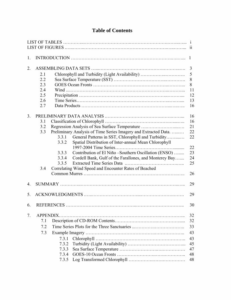
Table of Contents

LIST OF TABLES …………..………………………….…………………….……..…... i LIST OF FIGURES .…..……..……………………………………………….…..……... ii 1. INTRODUCTION ………………………………………………………….….…... 1 2. ASSEMBLING DATA SETS …...…………………………………….………..…. 3 2.1 Chlorophyll and Turbidity (Light Availability) ……………..…………. 5 2.2 Sea Surface Temperature (SST) ……………………………..…………. 8 2.3 GOES Ocean Fronts …………………………………………..………... 8 2.4 Wind ....………………………………………………………..………... 11 2.5 Precipitation …………………………………………………..………... 12 2.6 Time Series……………………………………………………..….….... 13 2.7 Data Products …………………………………………………...…..….. 16 3. PRELIMINARY DATA ANALYSIS .……………………………….…….……... 16 3.1 Classification of Chlorophyll …………………………………….…...….. 16 3.2 Regression Analysis of Sea Surface Temperature ….………………....…. 21 3.3 Preliminary Analysis of Time Series Imagery and Extracted Data. …...… 22 3.3.1 General Patterns in SST, Chlorophyll and Turbidity……....… 22 3.3.2 Spatial Distribution of Inter-annual Mean Chlorophyll

1997-2004 Time Series…………………………………......... 22

3.3.3 Contribution of El Niño –Southern Oscillation (ENSO) …..... 23 3.3.4 Cordell Bank, Gulf of the Farallones, and Monterey Bay….... 24 3.3.5 Extracted Time Series Data .…………………………….….. 25 3.4 Correlating Wind Speed and Encounter Rates of Beached

Common Murres …..………………………………………………….….. 26

4. SUMMARY …………..………………………………………………………..….. 29 5. ACKNOWLEDGMENTS .…..…………………………...………………….……. 29 6. REFERENCES ………………………………………..………………………….. 30 7. APPENDIX………………………………………………………….…………….. 32 7.1 Description of CD-ROM Contents……………………….……………..... 32 7.2 Time Series Plots for the Three Sanctuaries ...………….……………….. 33 7.3 Example Imagery ……………………………………….……………….. 43 7.3.1 Chlorophyll ….……………………………………………….. 43 7.3.2 Turbidity (Light Availability) ………………………………... 45 7.3.3 Sea Surface Temperature …………………….….…………… 47 7.3.4 GOES-10 Ocean Fronts …………………….…….………….. 48 7.3.5 Log Transformed Chlorophyll …………….…….…………… 48

List of Tables

1. Data and products generated……………………………………………………. 4

2. Extracted data for each type of dataset for the Gulf of the Farallones, Cordell Bank, and Monterey Bay National Marine Sanctuaries ………………..………. 15

i

List of Figures

1. Location map of the project study area …………………………………………………. 2 2. Examples of mean monthly SeaWiFS imagery ……………………………….…........... 6 3. Examples of mean monthly chlorophyll and log transform imagery……….................... 7 4. Examples of sea surface temperature imagery...……………………………….……….. 9 5. Examples of GOES ocean fronts imagery ……………………………………....……… 10

Frequency of winds from each octant by month (Jan=1, Dec=12) for the time 6. series1983-2004……………………………..……………………………….................. 11 7. Illustration of one-degree precipitation data with precipitation anomalies ………..….... 12 8. Location map for the eleven data extraction locations ………………………..………... 13

1997-2004 time series plots of for the Cordell Bank Sanctuary and 1997-2003 9. regional precipitation …………………………………………………………………… 14 K-Means unsupervised classification using inter-annual monthly mean 10. chlorophyll data from 1997-2004 ………………………………………………….…… 17

11. K-Means classification of 1997-1998 El Niño event …………………..…….………… 19 K-means classification of the inter-annual monthly mean chlorophyll data 12. without the 1997-1998 El Niño event …….……………………………………………. 20

13. Geographic variability of r2 for Farallones Light. and Hopkins Marine Lab SST ……... 21 14. 1997-2004 Time series of inter-annual monthly mean derived chlorophyll imagery .… 23 15. 1993-2003 Locations at which Common Murres were found ………………….….….... 26 16. Example scatter plot of monthly encounter rates and wind stress ………….……..……. 27 17. Example time series plot for deposition and quadrant 1-3 wind stress …….…..………. 28

Appendix A-1 Cordell Bank mean monthly chlorophyll time series plots ………………………..…… 33 A-2 Cordell Bank mean monthly turbidity time series plots ……………………………...… 34 A-3 Cordell Bank mean monthly sea surface temperature time series plots …………...…… 35 A-4 Gulf of Farallones mean monthly chlorophyll time series plots. …………………..…… 36 A-5 Gulf of Farallones mean monthly turbidity time series plots ………………………...… 37 A-6 Gulf of Farallones mean monthly sea surface temperature time series plots …….…….. 38 A-7 Monterey Bay mean monthly chlorophyll time series plots ……………………….…... 39 A-8 Monterey Bay mean monthly turbidity time series plots ……………………….……… 40 A-9 Monterey Bay mean monthly sea surface temperature time series plots ……….……… 41 A-10 Mean monthly precipitation for the southwest region …………………………….…… 42 A-11 Example geotiff chlorophyll imagery ………………………………………….………. 43 A-12 Example geotiff chlorophyll imagery, continued ……………………………….……… 44 A-13 Example geotiff turbidity imagery (RRS)670)) …………………………….………….. 45 A-14 Example geotiff turbidity imagery (RRS)670)), continued ………………….……........ 46 A-15 Sea surface temperatures …………………………………………………...................... 47 A-16 GOES-10 ocean fronts …………………………………………………………..……… 48 A-17 Standard deviations of log transformed chlorophyll ………………………….………... 48

ii

This project provides a framework for developing the capabilities of using satellite and related oceanographic and climatological data to improve environmental monitoring and characterization of physical, biological, and water quality parameters in the National Marine Sanctuaries (NMS). The project sought to:

1) assemble satellite imagery datasets in order to extract spatially explicit time series information on temperature, chlorophyll, and light availability for the Cordell Bank, Gulf of the Farallones, and Monterey Bay National Marine Sanctuaries.

2) perform preliminary analyses with these data in order to identify seasonal, annual,

inter-annual, and event-driven patterns. 1. Introduction Characterizing the distribution and variability of sea surface temperature (SST), chlorophyll, and light availability (turbidity) can be important to understanding the environmental conditions influencing the variability of the coastal and estuarine ecosystems in National Marine Sanctuaries. Variability in SST is a reflection of circulation and climate changes that may occur at episodic, seasonal and inter-annual time scales. Similarly, chlorophyll and turbidity distributions change in response to seasonal and inter-annual shifts in winds and precipitation, as well as specific storm events. Such variability over a large area is difficult to characterize from shipboard or moored measurements, but can be assessed from long-term, well-calibrated satellite data. The response of coastal systems to changes in natural forcing provides a benchmark for evaluating human impacts and helps determine the extent to which coastal zone management actions, such as erosion control and nutrient loading reductions, will lead to improvements in coastal ecosystem health and sustainability. The variability in water quality conditions over time can also be linked to changes observed in established surveys of living marine resources, including distributions of seabirds, fish, and marine mammals. These linkages may help to determine the conditions controlling these populations and provide information to improve resource management within the National Marine Sanctuaries. This study uses data from satellite and in situ sensors to characterize oceanographic conditions for the Gulf of the Farallones, Cordell Bank, and Monterey Bay National Marine Sanctuaries on the central California Coast (Figure 1). Chlorophyll and turbidity information from October 1997 to December 2004 are derived from Sea-viewing Wide Field-of-View Sensor (SeaWiFS) satellite ocean color data processed to 1-km spatial resolution. Satellite SST data (1985 to 2004) were obtained from the Advanced Very High Resolution Radiometer (AVHRR) with the climatological-grade Pathfinder calibration. Ancillary wind data were acquired from marine buoys operated by the National Oceanic and Atmospheric Administration (NOAA) and from gridded surface wind fields provided by the NOAA National Weather Service. Spatial patterns in the temperature, chlorophyll and turbidity fields were identified, as well as the variability in those patterns. Time series information was also extracted from the datasets to investigate trends at a variety of time-scales. This study demonstrates how satellite-based characterizations of oceanographic conditions can

1

effectively provide information for improved natural resource management in coastal ecosystems. The Gulf of the Farallones NMS encompasses an area of 948 square nautical miles and is situated to the west and northwest of San Francisco, CA. Approximately 52 miles from San Francisco, Cordell Bank NMS lies along the northwest border of the Farallones, covering 397 square nautical miles on the edge of the continental shelf. Located to the south of the Farallones, Monterey Bay NMS is the largest of the three marine sanctuaries covering 2024 nautical miles and extending 348 nautical miles southward from San Francisco.

Figure 1. Location map of the project study area.

2

2. Assembling Datasets Chlorophyll and turbidity products were derived from data obtained from the Sea-Viewing Wide Field-of-View Sensor (SeaWiFS) on the Orbview-2 satellite (operated by OrbImage Corp.). SeaWiFS data for research and educational applications has been available through the National Aeronautics and Space Administration (NASA) since its launch in September of 1997 through December 2004. NOAA has maintained a license for real-time civilian government use from September 1999 to the present. Data from this license (including after December 2004), can be used and distributed for civilian government operations only, and may not be distributed to the general research community. The sensor provides reliable daily observations for the coastal United States at a nominal spatial resolution of 1.1km for spectral bands encompassing the visible and near-infrared spectrum. Sea surface temperature (SST) data were received from the NASA Pathfinder Version 5.0 dataset. This dataset derives a climatological grade sea surface temperature product from Advanced Very High Resolution Radiometer (AVHRR) imagery, which was generated from several NOAA Polar-orbiting Environmental Satellites (POES) between 1985 and the present. Ocean fronts data, regions that delineate the boundary between different water masses, were obtained from the Geostationary Operational Environmental Satellite (GOES-10). Ancillary wind and precipitation data were also acquired. Monthly images were produced from daily images. The majority of the products were obtained as monthly and then binned to seasonal and inter-annual monthly means and medians. Seasonal images were created from the monthly mean images using the following seasonal breakdown: Fall—September, October, November Winter—December, January, February Spring—March, April, May Summer—June, July, August Spring and summer correspond to the upwelling season (March to August), fall corresponds to the relaxation season, and winter to the winter storm season. Time series images consist of all monthly mean or median data for each month over time. For example, the month of January has an image of mean chlorophyll for each of the years 1998 to 2004. These seven monthly images would be averaged to obtain the inter-annual mean of chlorophyll for this month for the 1998 to 2004 time series. All image data was subset to the specified region of interest and reprojected into Universal Transverse Mercator (zone 10). The majority of time invested in this project was devoted to data collection, processing, and the creation of output products. Table 1 summarizes these datasets.

3

Table 1: Data and products generated.

Data Type Daily Monthly SeasonalInter-

annual Monthly

Native Resolution Reformatting Product

Format

Chlorophyll and Available Light SeaWiFS

Chlorophyll 1997-2004

x x x x 1.1km data reprojection Geotiff

SeaWiFS Turbidity 1997-2004

x x x x 1.1km data reprojection Geotiff

Sea Surface Temperature and Fronts

Pathfinder SST

1985-2004 x x x 4km

1.1km resampling,

data reprojection

Geotiff

GOES Fronts

2001-2004 x x 3.36km

1.1km resampling,

data reprojection

Geotiff

Ancillary Data

CMAN Winds

1987-2003 x x hourly

observations

creation of 7day, 15day, and 30day

means

text files

Precipitation

1997-2003 x

monthly means on a

1 degree grid

spreadsheet

4

2.1 Chlorophyll and Turbidity (light availability) The ocean color dataset from SeaWiFS provided a seven-year (October 1997 to December 2004) time series of chlorophyll and light attenuation data. The Remote Sensing Team at the Center for Coastal Monitoring and Assessment (CCMA-RST) has developed algorithms, implemented by NASA for standard processing, to improve the generation of ocean color data and estimation of chlorophyll from SeaWiFS in the coastal zone (Stumpf et al., 2003).

The CCMA-RST has reprocessed the entire SeaWiFS dataset with SeaDAS version 4.5, applying the improved algorithms and obtaining georeferenced chlorophyll and light availability data at 1-km spatial resolution for all continental U.S. coastal regions. For this project, products were created for the central California region specifically to include the locations of the Cordell Bank, Gulf of the Farallones, and Monterey Bay sanctuaries (Figure 2). Estimations in chlorophyll in units of µg L-1 are derived using the standard OC4v4 equation that NASA used for global products from SeaWiFS. Accepted ‘chlorophyll’ algorithms such as OC4v4 for SeaWiFS measure chlorophyll-a. Chlorophyll-a is the dominant pigment in marine photosynthetic organisms, and is referred to simply as chlorophyll within this report. Turbidity is estimated using the remote sensing reflectance at 670nm Rrs(670) units of Steradian -1, which indicates red light reflected from the mean. At 670nm, pigment absorption is weak, and the reflectance indicates the scattering due to sediments. Thus, increased sediment concentrations will lead to higher reflectance (brighter water). Over the range of reflectance observed, Rrs(670) is nominally proportional to sediment concentrations. This band is particularly useful in identifying plumes of sediment-laden water from rivers or San Francisco Bay (Stumpf and Pennock, 1989). Time series image sets of chlorophyll and turbidity were created for the specified region in Geotiff format. These time series images are useful for determining trends in algal bloom activity and suspended sediment patterns. The final products were projected using the Universal Transverse Mercator (UTM) zone 10 north projection with the World Geodetic System 1984 (WGS-84) datum. The imagery time series generated from the SeaWiFS data includes monthly means which are 30-day average images, and monthly medians. Seasonal means and medians are monthly files used to create a seasonal image (seasons previously defined), and inter-annual monthly files are generated using all monthly images for a particular month in the time series as input.

Additionally, images using the standard deviation of the log transformed chlorophyll data were created to highlight areas of variability. Due to the nature of chlorophyll distributions, standard deviations of the untransformed data would resemble the mean. By using the standard deviation of the log transformed data, which does not co-vary about the mean, areas of higher variability are better described. This is significant for dynamic localized areas, where change may not otherwise be as well captured. This is illustrated in Figure 3. The log transform images show the percentage of variability of chlorophyll distributions.

5

(a)

(b) Figure 2: Samples of monthly mean SeaWiFS imagery. (a) Chlorophyll image from October 1997 in units of µg L-1, (b) Turbidity image from October 1997 in units steradian -1.

6

(a)

(b) Figure 3. Mean monthly chlorophyll and log transform images, December 1999. (a) Chlorophyll image in units of µg L-1, (b) Log transformed monthly chlorophyll by percent of variation. The images illustrate the high localized variability captured in the log transform image juxtaposed to mean chlorophyll. San Francisco Bay, an area of sustained high chlorophyll concentrations, has a correspondingly low range of variability.

7

2.2 Sea Surface Temperature (SST) Sea surface temperature (SST) information was acquired from the Pathfinder Version 5.0 SST dataset, derived from Advanced Very High Resolution Radiometer (AVHRR) satellite data. The Pathfinder dataset consists of seventeen years (1985 to 2001) of daily (excepting clouds) and monthly mean, climatological-grade georeferenced SST data for coastal U.S. waters. Interim data of the same quality was available for 2002 to 2004 from the National Oceanographic Data Center at NOAA (Figure 4). The Pathfinder dataset was calibrated for inter-comparison of the temperature data across the entire period, facilitating climate and other studies (NASA, 2004; NASA, 2005). Spatial resolution of the Pathfinder data varies slightly with latitude, with a horizontal resolution of about 4 km at 35 degrees of latitude. Pathfinder is distributed along a 0.04 degree grid in Cartesian coordinates. The original 4km data were resampled to 1.1km to match the spatial resolution of the SeaWiFS dataset and to create subsets of the same region as the chlorophyll and turbidity images. Geotiffs were created of the monthly mean time series (1985-2004) using the Universal Transverse Mercator (UTM) zone 10 north projection and the World Geodetic System 1984 (WGS-84) datum. SST image datasets were created from monthly means for the region. As was done for the chlorophyll and turbidity images, seasonal and inter-annual monthly means were generated. Units are degrees Celsius. The inter-annual monthly means consisted of the mean of a single month using all of the monthly mean files of that month throughout the time series. For example, the inter-annual monthly mean for January consisted of the average of all the monthly mean January images for the entire time series from 1985 to 2004. 2.3 GOES Ocean Fronts Ocean fronts are narrow areas of gradients of water temperature, salinity density and velocity. They delineate the boundary between different water masses, important off the California coast where the warmer California Current and cooler upwelling waters meet (Breaker, 2004). Monthly ocean frontal data were produced by NOAA Satellite and Information Service (NESDIS) from the Geostationary Operational Environmental Satellite GOES-10 for 2001 to 2004. The data were received in a binary format from NOAA’s Center for Satellite Applications and Research in Platte Carré or “Cartesian” coordinates with a vertical resolution of 5.5km per pixel. The data were resampled to 1.1km resolution to match the SeaWiFS products, and Geotiffs were created using the Universal Transverse Mercator (UTM) zone 10 north projection with the World Geodetic System 1984 (WGS-84) datum (Figure 5). The monthly images are probabilities of a front occurring at a given location during that month. These monthly images were then used to create seasonal means for the region. While the frontal data suggests fewer fronts in the winter, this is unlikely and best explained by the abundance of clouds. Clouds increase noise, significantly reducing detection of spatial features.

8

(a)

(b) Figure 4: Samples of sea surface temperature images in degrees Celsius. (a) Monthly mean sea surface temperature image from October 1985, (b) Seasonal sea surface temperature image for Fall 1985.

9

(a)

(b)

Figure 5: Examples of GOES ocean fronts imagery in units of probability of occurrence. (a) Monthly mean image from April 2001, (b) Seasonal image from spring 2001.

10

2.4 Wind Wind data were obtained from a Coastal-Marine Automated Network (C-MAN) buoy station 46026, located 18 nautical miles off the coast of San Francisco Bay, and operated by NOAA’s National Data Buoy Center (NOAA, 2005). This particular buoy was chosen because of its relative location in the region and its proximity to the shore. Wind speed and (meteorologic) direction, along with other meteorological parameters, were available hourly from 1983 to 2004. The data were divided into octants of 45 degrees to facilitate analysis of patterns in wind direction. The octants are clockwise sequentially from octant 1 at 0-45 degrees (NNE), octant 2 at 45-90 degrees (ENE), around to octant 8 at 315-360 degrees (NNW). Means of hourly observations were calculated at seven, fifteen, and thirty day intervals (Figure 6).

Figure 6: Frequency of winds from each octant by month (Jan=1, Dec=12) at the C-MAN station for the time series 1983-2004. The frequency axis in this case is the percent of total observations in a particular octant over the time period sampled.

11

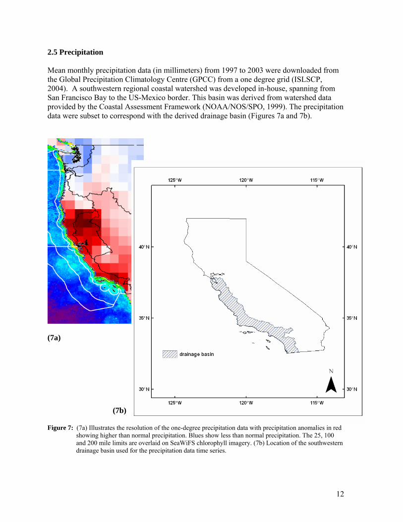
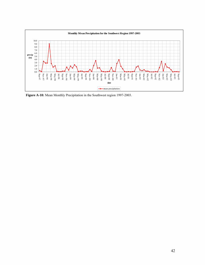
2.5 Precipitation Mean monthly precipitation data (in millimeters) from 1997 to 2003 were downloaded from the Global Precipitation Climatology Centre (GPCC) from a one degree grid (ISLSCP, 2004). A southwestern regional coastal watershed was developed in-house, spanning from San Francisco Bay to the US-Mexico border. This basin was derived from watershed data provided by the Coastal Assessment Framework (NOAA/NOS/SPO, 1999). The precipitation data were subset to correspond with the derived drainage basin (Figures 7a and 7b).

(7a)

(7b)

Figure 7: (7a) Illustrates the resolution of the one-degree precipitation data with precipitation anomalies in red showing higher than normal precipitation. Blues show less than normal precipitation. The 25, 100 and 200 mile limits are overlaid on SeaWiFS chlorophyll imagery. (7b) Location of the southwestern drainage basin used for the precipitation data time series.

12

2.6 Time Series The production of a consistent time series of imagery from the satellite datasets allowed for the extraction of data from each dataset at specific points, and for regional averages within the bounds of each sanctuary. These time series were extracted for eleven locations in the study region for preliminary analyses of episodic, seasonal and inter-annual patterns (Figure 8). Inter-annual monthly means were derived from the extracted time series.

Figure 8: Location map for the eleven data extraction locations. The flagged location is the C-MAN buoy station. The other colored points (boxes and rectangles) are the locations where data was extracted from the time series. Plots of data composited over the entire sanctuary, or for specific locations, were created as a way of making trends and anomalies in the data more easily identifiable (Figure 9). Table 2 shows the extracted datasets that were created from the time series data. These were created to aide in the process of identifying trends in the data and to highlight episodic and seasonal events that might be useful for future analysis. Preliminary analysis of the time series data is further discussed in section 3.

13

Mean Chlorophyll for Cordell Bank National Marine Sanctuary 1997-2004

0.01.02.03.04.05.06.07.08.0

Oct-97

Jan-98A

pr-98Jul-98

Oct-98

Jan-99A

pr-99

Jul-99O

ct-99Jan-00

Apr-00

Jul-00O

ct-00

Jan-01A

pr-01Jul-01

Oct-01

Jan-02A

pr-02

Jul-02O

ct-02Jan-03

Apr-03

Jul-03

Oct-03

Jan-04A

pr-04

Jul-04O

ct-04

date

chl (ug/L)

mean chl grand mean chl

Mean Turbidity for Cordell Bank National Marine Sanctuary 1997-2004

00.00020.00040.00060.0008

0.0010.0012

Oct-97

Jan-98A

pr-98Jul-98O

ct-98Jan-99A

pr-99Jul-99O

ct-99Jan-00A

pr-00Jul-00O

ct-00Jan-01A

pr-01Jul-01O

ct-01Jan-02A

pr-02Jul-02O

ct-02Jan-03A

pr-03Jul-03O

ct-03Jan-04A

pr-04Jul-04O

ct-04

date

670 (1/steradian)

mean 670 grand mean 670

Monthly Mean Precipitation for the Southwest Region 1997-2003

0.01.02.03.04.05.06.07.08.09.0

10.0

Sep-97

Dec-97

Mar-98

Jun-98

Sep-98

Dec-98

Mar-99

Jun-99

Sep-99

Dec-99

Mar-00

Jun-00

Sep-00

Dec-00

Mar-01

Jun-01

Sep-01

Dec-01

Mar-02

Jun-02

Sep-02

Dec-02

Mar-03

Jun-03

Sep-03

date

precip (in)

mean precipitation Figure 9: 1997-2004 time series plots of mean monthly chlorophyll, turbidity; and precipitation for the Cordell Bank Sanctuary from 1997-2003.

14

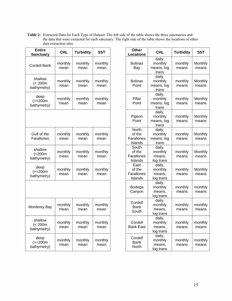
Table 2: Extracted Data for Each Type of Dataset. The left side of the table shows the three sanctuaries and the data that were extracted for each sanctuary. The right side of the table shows the locations of other data extraction sites.

Entire Sanctuary CHL Turbidity SST Other

Locations CHL Turbidity SST

Cordell Bank monthly mean

monthly mean

monthly mean Bolinas

Bay

daily, monthly

means, log trans

monthly means

Monthly means

shallow (< 200m

bathymetry)

monthly mean

monthly mean

monthly mean Bolinas

Point

daily, monthly

means, log trans

monthly means

Monthly means

deep (>=200m

bathymetry)

monthly mean

monthly mean

monthly mean Pillar

Point

daily, monthly

means, log trans

monthly means

Monthly means

Pigeon Point

daily, monthly

means, log trans

monthly means

Monthly means

Gulf of the Farallones

monthly mean

monthly mean

monthly mean

North of the

Farallones Islands

daily, monthly

means, log trans

monthly means

Monthly means

shallow (<200m

bathymetry)

monthly mean

monthly mean

monthly mean

South of the

Farallones Islands

daily, monthly means,

log trans

monthly means

Monthly means

deep (>=200m

bathymetry)

monthly mean

monthly mean

monthly mean

East of the

Farallones Islands


log trans

monthly means

Monthly means

Bodega Canyon


log trans

monthly means

monthly means

Monterey Bay monthly mean

monthly mean

monthly mean

Cordell Bank South


log trans

monthly means

monthly means

shallow (< 200m

bathymetry)

monthly mean

monthly mean

monthly mean Cordell

Bank East


log trans

monthly means

monthly means

deep

(>=200m bathymetry)

monthly mean

monthly mean

monthly mean

Cordell Bank North


log trans

monthly means

monthly means

15

2.7 Data Products This project has produced several data products for the end user. Complete sets of georeferenced images were produced with dates ranging from 1997 to 2004 for chlorophyll and turbidity, and from 1985 to 2004 for sea surface temperature. The CCMA-RST is also making available the ancillary wind data from 1983 to 2004, and precipitation data from 1997 to 2003. Federal Geographic Data Committee (FGDC) compliant metadata was created all imagery. All imagery, time series data, and metadata are available on the accompanying data CD-ROM. Refer to the appendix for examples of all image types and further discussion. 3. Preliminary Data Analysis

After processing the data, preliminary analysis were conducted in an effort to identify patterns exhibited in the datasets. Basic analysis includes classification maps of chlorophyll distributions, simple regression analysis of sea surface temperatures, time series analysis and correlation. 3.1 Classification of Chlorophyll We applied standard image classification techniques to the derived chlorophyll imagery products to characterize some of the driving factors in the local environment such as upwelling. This technique is typically applied to land-based datasets and rarely attempted for oceanographic applications. An unsupervised classification, using K-means clustering, was first performed on the inter-annual monthly mean chlorophyll imagery. Next, a separate K-means classification was performed on the monthly mean chlorophyll imagery from the strong El Niño year (1997-1998). A third classification was performed on an inter-annual mean, calculated from all chlorophyll data except that in the El Niño year. The latter classification attempted to assess the impact that the El Niño data had on the overall classification of the entire time series. This first classification identified some consistent spatial patterns in chlorophyll fields across the region (Figure 10a). Results indicated that features could indeed be identified along the coast based upon seasonal concentrations of chlorophyll. Plotting the classes identified through the classification helps to identify overall patterns that exist within the dataset (Figure 10b). The class colors used in the plot corresponded to those colors used in the imagery. For example, the red and orange classes (classes 1-4) tended to have less chlorophyll overall, while the light blue and green classes (classes 6-15) tended to have more throughout the time period, with purple and dark blue classes (classes 16-23) having the highest concentrations of chlorophyll. The areas circled in red were areas identified to be regions where upwelling was prominent based upon the shape of the class and the concentrations of chlorophyll.

16

(a)

1997-2004 Inter-Annual Monthly Mean Chlorophyll Classification - All Data

0.1

1

10

100

Jan Feb Mar Apr May Jun Jul Aug Sep Oct Nov Dec

date

chl

class1 class2 class3 class4 class5 class6 class7 class8class9 class10 class11 class12 class13 class14 class15 class16class17 class18 class19 class20 class21 class22 class23

(b) Figure 10: K-Means unsupervised classification using inter-annual monthly mean chlorophyll data from 1997-2004. (a) Classification color coded by class; (b) Corresponding classification table with the colors of each class corresponding to those in the classified image. The circled areas show different regions in San Francisco Bay (yellow circle) including the high chlorophyll, which peaks in March and April. The red circles mark the high upwelling areas with peaks in May. Monterey Bay is to the north, San Luis Obispo Bay to the south outside the sanctuary bounds.

17

The second classification, using the El Niño data (Figure 11), showed similar spatial patterns in general to the first classification, but with differences. The classes identified near San Francisco Bay are distinct from the surrounding classes, but there is not as much variability within those classes as with the first classification. The other regions we identified as upwelling regions in the first classification exist during the El Niño, but are not as prominent, indicating that upwelling might not be as strong during a strong El Niño event. More speckling is evident throughout the class regions in this classification, an indication of more noise in the dataset. The extreme cloud cover significantly reduced the number of usable pixels for this analysis if February and March, so they were excluded. We can also see that the peaks in chlorophyll tend to be in the spring, whereas in the first classification there were peaks in chlorophyll during the spring and the fall. The third classification (Figure 12) based on the inter-annual monthly mean data, excludes the El Niño year, thereby giving a better representation of the non-El Niño pattern. This classification shows not as much variability in the classes within San Francisco Bay (circled in yellow) indicating that the exclusion of the El Niño data removed some of the variability in chlorophyll in this area. San Francisco Bay (blue to purple classes 14-23) peaks in March and April, consistent with late winter rains and early spring runoff. The upwelling area is captured by classes 5-13; with the intensity increasing with class numbers. Peak chlorophyll in the upwelling zone occurs in April and May. The most intense features are in the Bays behind Points, especially Monterey Bay and San Luis Obispo Bay to the south of the Monterey Bay NMS.

Class 5 (the yellow class) is not as pronounced in the northern part of the image and is more so in the southern part. This shows that the El Niño had an impact on this class, indicating that this classification is more indicative of the conditions that exist there under more neutral circumstances. The upwelling regions also appear more pronounced as they did in the first classification. This type of analysis shows the utility of these types of remote sensing techniques to identify temporal and spatial patterns in oceanographic characteristics. Looking at events such as El Niño separately within the dataset also gives us episodic events that we can compare to the norm and investigate further.

18

(a)

El Nino 97-98 Monthly Mean Chlorophyll Classification

0.1

1

10

100

Oct-97 Nov-97 Dec-97 Jan-98 Feb-98 Mar-98 Apr-98 May-98 Jun-98

date(no data for February)

chl

class 1 class 2 class 3 class 4 class 5 class 6 class 7class 8 class 9 class 10 class 11 class 12 class 13 class 14class 15 class 16 class 17 class 18

(b) Figure 11: K-Means classification of 1997-1998 El Niño data. (a) The classification image displaying patterns for the El Niño event color coded by class; (b) The corresponding classification table showing chlorophyll concentrations per class throughout the El Niño event color coded to match the classified image. Monterey Bay is to the north, San Luis Obispo Bay to the south outside the sanctuary bounds.

19

(a)

1997-2004 Inter-Annual Monthly Mean Chlorophyll-No El Nino

0.1

1

10

100

Jan Feb Mar Apr May Jun Jul Aug Sep Oct Nov Dec

date

chl

class1 class2 class3 class4 class5 class6 class7 class8class9 class10 class11 class12 class13 class14 class15 class16class17 class18 class19 class20 class21 class22 class23

(b) Figure 12: K-means classification of the inter-annual monthly mean chlorophyll data without the El Niño months. (a) The classification image showing patterns of chlorophyll color coded by class; (b) The corresponding classification table with the classes plotted showing the patterns of chlorophyll throughout the time series color coded to match the classified image. San Francisco is circled in yellow corresponding to classes 14-23; red circles are Monterey Bay and San Luis Obispo to the south.

20

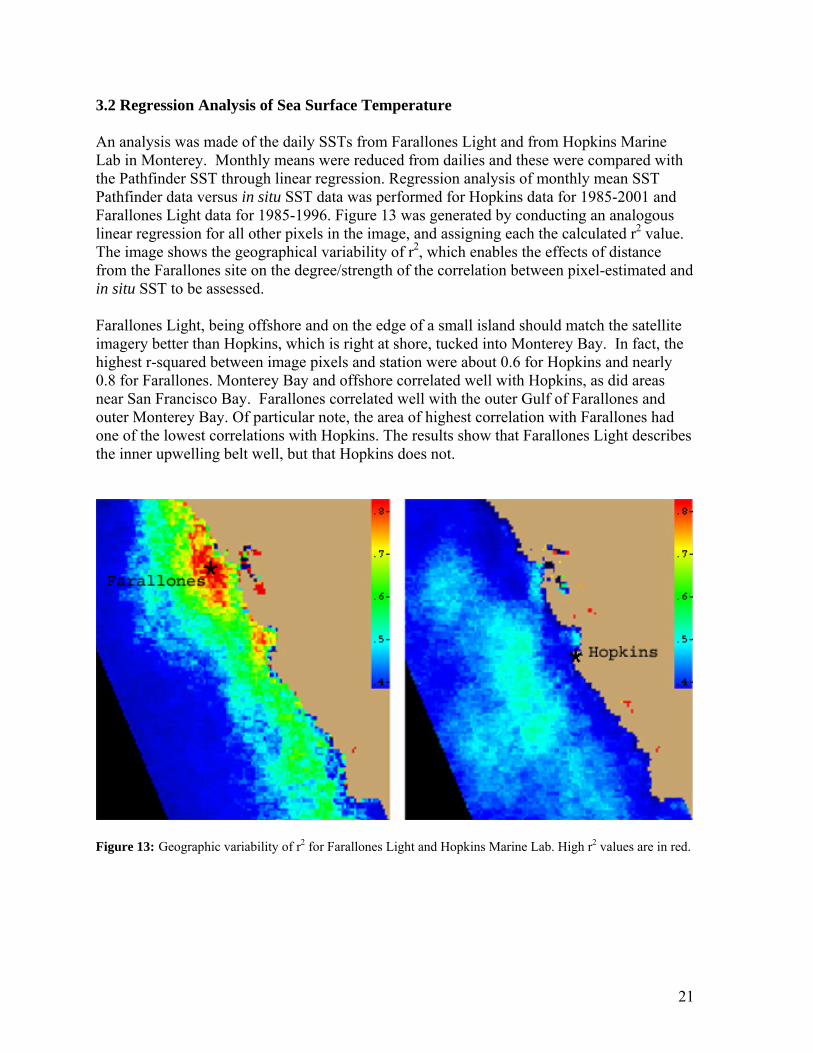
3.2 Regression Analysis of Sea Surface Temperature An analysis was made of the daily SSTs from Farallones Light and from Hopkins Marine Lab in Monterey. Monthly means were reduced from dailies and these were compared with the Pathfinder SST through linear regression. Regression analysis of monthly mean SST Pathfinder data versus in situ SST data was performed for Hopkins data for 1985-2001 and Farallones Light data for 1985-1996. Figure 13 was generated by conducting an analogous linear regression for all other pixels in the image, and assigning each the calculated r2 value. The image shows the geographical variability of r2, which enables the effects of distance from the Farallones site on the degree/strength of the correlation between pixel-estimated and in situ SST to be assessed. Farallones Light, being offshore and on the edge of a small island should match the satellite imagery better than Hopkins, which is right at shore, tucked into Monterey Bay. In fact, the highest r-squared between image pixels and station were about 0.6 for Hopkins and nearly 0.8 for Farallones. Monterey Bay and offshore correlated well with Hopkins, as did areas near San Francisco Bay. Farallones correlated well with the outer Gulf of Farallones and outer Monterey Bay. Of particular note, the area of highest correlation with Farallones had one of the lowest correlations with Hopkins. The results show that Farallones Light describes the inner upwelling belt well, but that Hopkins does not.

Figure 13: Geographic variability of r2 for Farallones Light and Hopkins Marine Lab. High r2 values are in red.

21

3.3 Preliminary Analysis of Time Series Imagery and Extracted Data Preliminary analysis was conducted on the three sanctuary regions. In addition to examining the sanctuary areas as a whole, eleven point locations were extracted from the imagery within the sanctuary boundaries. The point locations were chosen based upon interest expressed either by the end user or because these locations were considered representative of occurrences within the sanctuary bounds.

3.3.1 General Patterns in SST, Chlorophyll and Turbidity The time series imagery shows that the seasonal variation is driven by upwelling and non-upwelling seasons. The minimum sea surface temperature occurs in April and May as a result of seasonal cooling and upwelling, the maximum sea surface temperature in September is indicative of seasonal warming. Chlorophyll concentrations peak in April and May, but persist through September, consistent with the upwelling. Turbidity is more variable with a tendency to a minimum in December over the entire Sanctuaries. Near-coastal areas that are directly influenced by river plumes may show a maximum during the winter rainy season; however, this impact does not transfer over the entire shallow water (< 200 m) area. Figure 14 illustrates the measurement and spatial distribution of the inter-annual monthly mean derived chlorophyll for the1997-2004 time series of the coast of central California. The 1996 El Niño had a strong influence on river plumes (Mertes and Warrick, 2001). 3.3.2 Spatial Distribution of Inter-annual Mean Chlorophyll 1997-2004 Time Series. The images shown in Figure 14 illustrate the dynamic nature of the spatial distribution of monthly chlorophyll. The highest mean chlorophyll counts are darker warm colors and lower values are depicted by cooler colors decreasing from greens to blues. Mean chlorophyll concentrations have broad temporal variability. The California coast is bounded by the southward flowing California current. Upwelling in the study area occurs during the March through September contributing to an increase in nutrient enriched waters (Kudela and Chavez, 2004). This in turn contributes to an increase in algal blooms. This is evidenced in the time series images as abundant pigments indicate a strong spring bloom occurring in March and continuing to increase into the summer months. The increase in near-shore chlorophyll concentrations at this time corresponds with increasingly lower observations over time in deeper offshore waters. San Francisco Bay sustains relatively high chlorophyll levels year round due to eutrophication (Cloern, 1996). As the fall and winter months approach, increased cloud cover occurs and is most prevalent during winter months. This is a period of decreased light availability and PAR and coincides with the end of the upwelling season in October. The occurrence of some speckling in the imagery is attributed to the contribution that cloud cover makes to the image processing, and is most apparent during winter months.

22

Figure 14: 1997-2004 Inter-annual monthly mean derived chlorophyll. From top to bottom, column 1 depicts January, February March and April images; column 2 May, June, July and d August; and column 3 September, October, November and December. 3.3.3 Contribution of El Niño –Southern Oscillation (ENSO) The El Niño phenomenon is an important factor influencing upwelling along this coast. The El Niño reduces upwelling intensity and the La Niña increases it. During the time series four El Niño events occurred in: 1987, late 1991- early 1992, late 1997-early 1998, and late 2002 (National Weather Service, 2005). The 1997-98 was possibly the most intense in the 20th century. La Niña events occurred in 1988 early 1989, and late 1998-2000. Of the El Niño events, the 1991-92 and 1997-98 produced strongly elevated SST in the three Sanctuaries. The others produced weak increases in SST. The 1991 and 1999 La Niña events led to much more intense upwelling as shown by the low temperatures. In chlorophyll the 1997-98 El Niño led to much lower chlorophyll concentrations than normal in all the Sanctuaries. This is expected and was reported by Kahru and Mitchell (2000). The 1999 La Nino produced some increase in chlorophyll, but not significant compared to other events.

23

3.3.4 Cordell Bank, Gulf of Farallones, and Monterey Bay Trends in the chlorophyll, sea surface temperature, and turbidity data were identified for the northernmost sanctuary. Both shallow (less than 200 m) and deep areas (greater than 200 m) showed similar phenomenon in temperature over the time with the major perturbations caused by the 1991-92 and 1997-98 El Niño and the 1999 La Niña. Annual temperature variations are similar, 11.3 to 14 ºC for the deep Sanctuary and 10.7 to 13.9 ºC in the shallow Sanctuary. The minimum is in May and the maximum in September in both areas. The spring minimum includes both seasonal and upwelling cooling, the September indicates seasonal warming. Different patterns appear in chlorophyll and turbidity. Cordell shows a seasonal pattern in turbidity with higher turbidity from March to June and lower from August to January consistent with the seasonal variation in precipitation, and river runoff. Offshore has the lower turbidity, but there is no significant patterns evident with the climate signal. The chlorophyll varies, on average from 4 to 11 µg L-1 in shallow areas and from 1 to 3 µg L-1 in deep water. Mean chlorophyll in the entire Sanctuary varies between 2 and 6 µg L-1. While the chlorophyll shows the impact of the El Niño in significantly reducing primary productivity, the major increases in chlorophyll are not tied to the La Niña. In 2001 the chlorophyll peaked in the shallow areas at nearly 20 µg L-1. This appears to owe to an intrusion of nutrient-rich sub-arctic water into the California current in 2002 (Thomas et al, 2003). The highest chlorophyll occurs in the Point Reyes area, as do the lowest temperatures. This region is comparable to Monterey Bay and the area south of Pt San Luis to Cape Conception in the elevated chlorophyll. The Farallones shows a mean range in temperature with negligible difference between the deep and shallow areas (deep 11.4 to 14.4 ºC, shallow from 11.5 to 14.7 ºC). However, the variability differs between shallow and deep areas, with greater variability in the shallow region producing most of the variability in the Sanctuary. Some impacts in precipitation have to be inferred. The shallow area of the Farallones is the most turbid of the three with mean reflectance of about 0.008 steradian -1. This is consistent with the impact of the plume from San Francisco Bay within the Gulf. Chlorophyll in the Farallones varies on average between 10 and 17 µg L-1 with the deep water regions have considerable variability from quite low (0.3 µg L-1) to 4 µg L-1. Monterey Bay shows a variation in the deep water SST of 12 to 15 ºC and 12.5 to 17 ºC in shallow water. Certain years show marked differences however. For example in 2002 and 2003 the deep-water was less than 1 ºC below average, shallow reached 2 ºC below average. Both the 1992 and 1998 El Niño events influenced shallow and deep water areas, as did the 1999 La Niña. The strongest variations in chlorophyll are the 1998 El Niño, which decreased chlorophyll, and the 2004 spring event, which had high chlorophyll concentrations. Turbidity shows a seasonal pattern of low in the winter and spring, and high in the summer/

24

3.3.5 Extracted Time Series Data Trends in the chlorophyll, turbidity, and sea surface temperature data can be identified for the three marine sanctuaries (Appendix Figures; Cordell A-1:A-3, Farallones A-4:A-6, Monterey A-7:A-9). In the northern most sanctuary, Cordell Bank, both turbidity and chlorophyll peaked during times of cooler than average sea temperatures. This is characteristic of an upwelling event. Periods of increased precipitation are associated with some increases (Appendix; Figure A-10), which could be responsible for the spikes in turbidity as re-suspended sediment in the coastal water. Spikes throughout the time series in early summer could be associated with seasonal characteristics of the California Current which has its maxima in summer and early fall. Strong upwelling occurs during the latter years. The California Current is a year-round equator-ward flow extending seaward from the shelf break to a distance of about 1000km with strongest speeds at the surface and extending at least to 500m in depth. It is characterized by strong seasonality in wind forcing, where during the winter months mean wind stress is poleward and downwelling-favorable. During the summer months the mean wind stress is equator ward and upwelling-favorable bring in cold, nutrient-rich water to the region (Bograd, 2005; Thomas, Strub, and Brickley, 2003). Looking at the sea surface temperature data regionally as well as in the shallow (less than 200m bathymetry) and deep (greater than 200m bathymetry) regions indicates that the shallow region is responsible for most of the variability in the regional mean plot for the Gulf of the Farallones sanctuary. Peaks in turbidity and chlorophyll with lower sea surface temperatures indicate upwelling conditions. Again, higher precipitation is associated with many occurrences which could account for some of the increase in turbidity. Nutrient run-off could also account for some of the increased chlorophyll in the coastal zone. Overall, Farallones appears to be an area more turbid than either Cordell Bank or Monterey. In the Monterey Bay sanctuary several peaks appear to occur both in and off shore, whereas other peak periods favor offshore areas. Based upon analysis of the deep and shallow plots this is most likely a function of the bathymetry in the sanctuary. For sea surface temperature, the deep and shallow plots appear to have more variability than the sanctuary taken as a whole. Throughout the three sanctuaries lower than average chlorophyll values were observed from the beginning of the SeaWiFS (late 1997) mission due to the impact of a strong El Niño event. The California Current appears to have the strongest impact on the Cordell Bank National Marine Sanctuary; however Farallones and Monterey also exhibit characteristics that correspond to its cycle.

25

3.4 Correlating Wind Speed and Encounter Rates of Beached Common Murres Wind speed seems to be the principal factor determining long distance carcass movement while currents, especially tidal currents, may influence deposition on specific beaches once the drifting carcass approaches the shore (Wiese and Jones, 2001). It was hypothesized that in times of increased wind speeds more bird carcasses would be transported in-inshore, thereby contributing to a greater deposition of dead birds than the number found during times of lower wind speeds. To investigate a possible correlation between deposition rates and wind speed, historic shoreline surveys (Roletto, et al., 2005) and wind data for the period September 1993 to September 2000 were compared. The survey data used in the analysis were collected from beach segments beginning in the north at Doran Beach in Sonoma County, and going southward to Bradley Beach in San Mateo County (Figure 15).

Figure 15: 1993-2003 Locations at which Common Murres were found. Shoreline surveys of bird carcass deposition were collected by the Gulf of the Farallones National Marine Sanctuary Beach Watch Program. Following the lead of the Beach Watch annual report, data pertaining specifically to the Common Murre were used to look at the relationship between carcass deposition rates and wind. Murres, which maintain a year-round presence in the area, are the most encountered beached birds (Roletto et al., 2000). Additionally, the size of the Murre lends to finding the carcasses because smaller birds tend to be more easily scavenged. This analysis uses the total monthly deposition rates of bird carcasses found within the study area.

26

Wind speed data came from the National Buoy Data Center (NDBC) Station 46026 located 18 miles northwest of San Francisco, CA (37°45'32" N 122°50'00" W). Wind speed direction is meteorologic (the direction from which wind is blowing). From wind speed, average monthly nominal wind stress (square of the wind speed) was derived for each of the four quadrants (NE, SE, SW, and NW). Wind stress was used instead of wind speed because it takes into consideration the drag produced by wind on currents and drifting animals. Therefore, when considering wind driven transport, winds of greater velocity are given exponentially more weight than those of lesser velocity. Simple statistics and visual analysis of graphic plots were used to look for a correlation between wind speed and Murre deposition rates. The total number of dead birds found per month along the coastline was plotted against the monthly wind stress in scatter plots, both by individual quadrant and by total wind stress within multiple quadrants (Figure 16). Regardless of the quadrant against which beached Murres were plotted, greater numbers were surveyed during periods of lower wind speed. The average number of surveyed Murres per month was 27.5 over the seven year period. Above average rates, and in particular numbers of greater than 100 occurred when the nominal wind stress was less than 20 m2 / sec2 in the cases of the NE, SE, and SW quadrants or during the winter of the 1997-98 El Niño. Outliers occurred during the months of November 1997 to February 1998. For the NW quadrant, where wind totals are typically larger, greater numbers were surveyed when wind stress was less than 80 m2 / sec2. For all quadrants frequent occurrences (> 15) were found during the major El Niño and during low wind stress from the NE, SE, and SW quadrants.

Monthly Total Beach Deposition of Common Murres vs. Wind Stress of SW Quandrant September 1993 - September 2000

0

20

40

60

80

100

120

140

160

180

0 20 40 60 80 100 120

30 Day Total Weighted Nominal Wind Stress m2/sec2

# Fo

und

Dea

d

1997-98 El Nino outliers

Figure 16: Example scatter plot of monthly encounter rates and wind stress.

27

This observation seems to indicate some negative correlation (lower wind speeds and higher deposition rates), but there is only a weak linear relationship. A non linear response appears to occur with more frequent observed beachings at < 20 m2/sec2

and fewer (generally) for > 20 m2/sec2. The correlation coefficients of the wind stress and deposition rates for the four quadrants are slightly negative (r = -.19, -.20, -.17, and -.29 respectively). Similar correlation was found when plotting deposition rates with the aggregated wind stress of NE, SE, and SW quadrants (r = -.27) and all quadrants (r = -.21). The initial supposition was that beached Murre encounter rates would be higher during periods of increased wind speeds. This has not been shown to be true; in fact a slightly negative, but not necessarily significant correlation exists between the data. To look for obvious trends or patterns in the data, the monthly deposition rates and monthly wind data for all seven years were plotted as times series (Figure 17). As evidenced in the scatter plots, there seems to be an apparent trend that shows the inverse relationship between encounter rates and wind speed. This is evident throughout the time series for all quadrants, but most strongly expressed when plotting wind stress of NW quadrant. An exception to this generally inverse relationship is the fall 1997 and winter 1998 months. At this time both wind speed and encounter rates increase. This increase in encounter rates is during the major El Niño and also corresponds with the Point Reyes Tar Ball Incident. Generally speaking it is expected that Murre encounter rates will increase during the post-breeding period of August through October (Roletto, et al., 2000). This trend is shown in the data, and corresponds with periods of weaker winds.

Beached Common Murres and Wind Stress in Quadrants NE, SE, SWSeptember 1993 - September 2000 T ime Series

0

20

40

60

80

100

120

140

160

180

Sep

-93

Dec

-93

Mar

-94

Jun-

94

Sep

-94

Dec

-94

Mar

-95

Jun-

95S

ep-9

5D

ec-9

5M

ar-9

6Ju

n-96

Sep

-96

Dec

-96

Mar

-97

Jun-

97

Sep

-97

Dec

-97

Mar

-98

Jun-

98

Sep

-98

Dec

-98

Mar

-99

Jun-

99S

ep-9

9D

ec-9

9M

ar-0

0

Jun-

00S

ep-0

0

# Fo

und

Dea

d

-10

0

10

20

30

40

50

60

70

80

90

30 D

ay W

eigh

ted

Win

d Sp

eed

m2 /sec

2

# Found per Month Wind Stress Q1-Q3

Figure 17: Example time series plot for deposition and quadrant 1-3 wind stress.

28

4. Summary This report identifies the key objectives of this project and how they were met through the creation of GIS compatible geotiff products of chlorophyll, turbidity, and sea surface temperature. Additional GOES ocean front and CMAN Wind data are provided. This report also provides preliminary analysis illustrative of the utility of this data for a variety of analyses to characterize oceanographic conditions in the National Marine Sanctuaries on the central California Coast. This study demonstrates how satellite-based characterizations of oceanographic conditions can effectively provide information to improve natural resource management in coastal ecosystems. 5. Acknowledgements We would like to thank Tim Mavor of NOAA/NESDIS Office of Research and Applications for providing the GOES-10 ocean front analysis; Kenneth Casey, of NOAA National Oceanographic Data Center for providing the Pathfinder SST data before it was commonly available; and Jan Roletto of the Gulf of the Farallones National Marine Sanctuary for providing the Beach Watch bird survey data used in our preliminary analysis.

29

6. References Bograd, S.J. 2005. California Current. [available online] http://www.pices.int/publications/ special_publications/NPSER/2005/File_10_pp_177_192.pdf. Breaker, L. 2004. Ocean Fronts off California: A New Product from GOES Satellite Data. Coastal Ocean Research. R/CZ-181:3.1.2002-2.28.2005. [Available online] http://www-csgc.ucsd.edu/RESEARCH/PROJPROF_PDF/RCZ181.pdf. Cloern, J.E. 1996. Phytoplankton Bloom Dynamics in Coastal Ecosystems: A Review with Some General Lessons from Sustained Investigation of San Francisco Bay, California. Review of Geophysics. 34:127-168. ISLSCP (International Satellite Land Surface Climatology Project). 2004. Global Precipitation Climatology Centre (GPCC) Monthly Precipitation. [Available online] http://islscp2.sesda.com/ISLSCP2_1/html_pages/groups/hyd/gpcc_precip_monthly_xdeg.html. Kahru, M. and B.G. Mitchell, 2000. Influence of the 1997-1998 El Niño on the Surface Chlorophyll in the California Current. Geophysical Research Letters. 27:2937-2940. Kudela and Chavez, 2004. The Impact of Coastal Runoff on Ocean Color during an El Niño year in Central California. Deep Sea Research. [in press] Mertes, L.A.K., and J.A. Warrick, 2001. Measuring Flood Output from 110 Coastal Watersheds in California with Field Measurements and SeaWiFS. Geology. V. 29 7:659-662. NASA. 2004. AVHRR Oceans Pathfinder Sea Surface Temperature Datasets. [Available online] http://podaac.jpl.nasa.gov:2031/DATASET_DOCS/avhrr_pathfinder_sst_v5.html. NASA 2005. AVHRR Pathfinder Documentation. [Available online] http://podaac.jpl.nasa.gov/sst/sst_doc.html. NOAA/NOS/SPO. 1999. Coastal Assessment Framework, N/SPO, 9th Floor 1305 East-West Highway, Silver Spring, MD 20910, USA. NOAA. 2004. NOAA-CIRES Climate Diagnostics Center. [available online] http://www.cdc. noaa.gov/. NOAA. 2005. National Data Buoy Center. [available online] http://www.ndbc.noaa.gov/. National Weather Service, 2005. Cold and Warm Episodes by Season. http://www.cpc.ncep.noaa.gov/products/analysis_monitoring/ensostuff/ensoyears.shtml Roletto, J., J. Mortenson, L. Frella, and L. Culp, 2000. Beach Watch Annual Report: 2000. Unpublished report to the National Oceanic and Atmospheric Administration, Gulf of the Farallones National Marine Sanctuary, San Francisco, CA.

30

Roletto, J, J. Mortenson, J. Hall and S. Lyday, 2005. Beach Watch Annual Report: 2004. Unpublished report to the National Oceanic and Atmospheric Administration, Gulf of the Farallones National Marine Sanctuary, San Francisco, CA. Stumpf, R.P. and J.R. Pennock. 1989. Calibration of a general optical equation for remote sensing of suspended sediments in a moderately turbid estuary. Journal of Geophysical Research Oceans. 94 (10): 14363-14371. Stumpf, R.P., R.A. Arnone, R.W. Gould, Jr., P. Martinolich, and V. Ransibrahmanakul. 2002. A Partially-Coupled Ocean-Atmosphere Model for Retrieval of Water-Leaving Radiance from SeaWiFS in Coastal Waters: In: Patt, F.S., and et al., 2002: Algorithm Updates for the Fourth SeaWiFS Data Reprocessing. NASA Tech. Memo. 2002-206892, Vol. 22, S.B. Hooker and E.R. Firestone, Eds., NASA Goddard Space Flight Center, Greenbelt, Maryland. Thomas, A.C., P.T. Strub, P. Brickley, 2003. Anomalous satellite-measured chlorophyll concentrations in the northern California Current in 2001-2002. Geophysical Research Letters, 30(15): 8022. Wiese, F.K. and I.L. Jones, 2001. Experimental Support for a New Drift Block Design to Assess Seabird Mortality from Oil Pollution. The Auk: Vol. 18, No. 4, pp. 1062-1068.

31

7. Appendix 7.1 Description of CD-ROM Contents This project has produced several dataset products for the end user. The accompanying CD-ROM contains all of the GIS compatible data products created for this project. Complete sets of georeferenced Geotiff images are included for the 1997 to 2004 chlorophyll and turbidity, and 1985 to 2004 sea surface temperature data. Due to the large volume of data, daily chlorophyll and turbidity imagery has been compressed by year using WinZip software. Extracted time series data are included in Excel spreadsheet format. Additionally, the CCMA-RST is making available the ancillary CMAN wind data from 1983 to 2004 in text file format, precipitation data from 1997 to 2003 in Excel spreadsheet format, and GOES ocean front data for 2001-2004 as Geotiff imagery. Federal Geographic Data Committee (FGDC) compliant metadata was created for all image products. All imagery, extracted and derived time series, chlorophyll classification maps, and metadata are available on the accompanying data CD-ROM. Examples of the each dataset are included within sections 7.2 and 7.3 of this appendix.

32

7.2 Time Series Plots for the Three Sanctuaries

Mean Chlorophyll for Cordell Bank National Marine Sanctuary 1997-2004

0.01.02.03.04.05.06.07.08.0

Oct-97

Jan-98

Apr-98

Jul-98

Oct-98

Jan-99

Apr-99

Jul-99

Oct-99

Jan-00

Apr-00

Jul-00

Oct-00

Jan-01

Apr-01

Jul-01

Oct-01

Jan-02

Apr-02

Jul-02

Oct-02

Jan-03

Apr-03

Jul-03

Oct-03

Jan-04

Apr-04

Jul-04

Oct-04

date

chl (ug/L)


(a)

Mean Chlorophyll for Cordell Bank National Marine Sanctuary Shallow (<200m bathymetry) 1997-2004

0.0

5.0

10.0

15.0

20.0

25.0

Oct-97

Jan-98

Apr-98

Jul-98

Oct-98

Jan-99

Apr-99

Jul-99

Oct-99

Jan-00

Apr-00

Jul-00

Oct-00

Jan-01

Apr-01

Jul-01

Oct-01

Jan-02

Apr-02

Jul-02

Oct-02

Jan-03

Apr-03

Jul-03

Oct-03

Jan-04

Apr-04

Jul-04

Oct-04

date

chl (ug/L)


(b)

Mean Chlorophyll for Cordell Bank National Marine Sanctuary Deep (>200m bathymetry) 1997-2004

0.0

2.0

4.0

6.0

8.0

Oct-97

Jan-98

Apr-98

Jul-98

Oct-98

Jan-99

Apr-99

Jul-99

Oct-99

Jan-00

Apr-00

Jul-00

Oct-00

Jan-01

Apr-01

Jul-01

Oct-01

Jan-02

Apr-02

Jul-02

Oct-02

Jan-03

Apr-03

Jul-03

Oct-03

Jan-04

Apr-04

Jul-04

Oct-04

date

chl (ug/L)


(c) Figure A-1: Cordell Bank Mean Monthly Chlorophyll in (a) Region, (b) Shallow waters, and (c) Deep waters

33

Mean Turbidity for Cordell Bank National Marine Sanctuary 1997-2004

00.00020.00040.00060.00080.001

0.0012

Oct-97

Jan-98

Apr-98

Jul-98

Oct-98

Jan-99

Apr-99

Jul-99

Oct-99

Jan-00

Apr-00

Jul-00

Oct-00

Jan-01

Apr-01

Jul-01

Oct-01

Jan-02

Apr-02

Jul-02

Oct-02

Jan-03

Apr-03

Jul-03

Oct-03

Jan-04

Apr-04

Jul-04

Oct-04

date

670 (1/steradian)


(a)

Mean Turbidity for Cordell Bank National Marine Sanctuary Shallow (< 200m bathymetry) 1997-2004

00.00050.001

0.00150.002

0.00250.003

Oct-97

Jan-98

Apr-98

Jul-98

Oct-98

Jan-99

Apr-99

Jul-99

Oct-99

Jan-00

Apr-00

Jul-00

Oct-00

Jan-01

Apr-01

Jul-01O

ct-01

Jan-02

Apr-02

Jul-02O

ct-02

Jan-03

Apr-03

Jul-03O

ct-03

Jan-04

Apr-04

Jul-04O

ct-04

date

670 (1/steradian)


(b)

Mean Turbidity for Cordell Bank National Marine Sanctuary Deep (> 200m bathymetry) 1997-2004

00.00010.00020.00030.00040.00050.00060.00070.0008

Oct-97

Jan-98

Apr-98

Jul-98

Oct-98

Jan-99

Apr-99

Jul-99

Oct-99

Jan-00

Apr-00

Jul-00

Oct-00

Jan-01

Apr-01

Jul-01O

ct-01

Jan-02

Apr-02

Jul-02O

ct-02

Jan-03

Apr-03

Jul-03O

ct-03

Jan-04

Apr-04

Jul-04O

ct-04

date

670 (1/steradian)


(c) Figure A-2: Cordell Bank Mean Monthly Turbidity in (a) Region, (b) Shallow Waters, and (c) Deep Waters

34

Mean Sea Surface Temperature for Cordell BankNational Marine Sanctuary 1985-2004

8.010.012.014.016.018.020.0

Jan-85Jul-85Jan-86Jul-86Jan-87Jul-87Jan-88Jul-88Jan-89Jul-89Jan-90Jul-90Jan-91Jul-91Jan-92Jul-92Jan-93Jul-93Jan-94Jul-94Jan-95Jul-95Jan-96Jul-96Jan-97Jul-97Jan-98Jul-98Jan-99Jul-99Jan-00Jul-00Jan-01Jul-01Jan-02Jul-02Jan-03Jul-03Jan-04Jul-04

date

sst (deg C)

mean sst grand mean sst

(a)

Mean Sea Surface Temperature for Cordell Bank National Marine Sanctuary Shallow(<200m bathymetry) 1985-2004

8.010.012.014.016.018.020.0

Jan-85Jul-85Jan-86Jul-86Jan-87Jul-87Jan-88Jul-88Jan-89Jul-89Jan-90Jul-90Jan-91Jul-91Jan-92Jul-92Jan-93Jul-93Jan-94Jul-94Jan-95Jul-95Jan-96Jul-96Jan-97Jul-97Jan-98Jul-98Jan-99Jul-99Jan-00Jul-00Jan-01Jul-01Jan-02Jul-02Jan-03Jul-03Jan-04Jul-04

date

sst (deg C)


(b)

Mean Sea Surface Temperature for Cordell Bank National Marine Sanctuary Deep (>200m bathymetry) 1985-2004

8.0

10.0

12.0

14.0

16.0

18.0

20.0

Jan-85Jul-85Jan-86Jul-86Jan-87

Jul-87Jan-88Jul-88Jan-89Jul-89







date

sst (deg C)


(c)

Figure A-3: Cordell Bank Mean Monthly Sea Surface Temperature in (a) Region, (b) Shallow Waters, and (c) Deep Waters

35

Mean Chlorophyll for Gulf of the Farallones National Marine Sanctuary 1997-2004

0.02.04.06.08.0

10.012.014.016.0

Oct-97

Jan-98

Apr-98

Jul-98

Oct-98

Jan-99

Apr-99

Jul-99

Oct-99

Jan-00

Apr-00

Jul-00

Oct-00

Jan-01

Apr-01

Jul-01

Oct-01

Jan-02

Apr-02

Jul-02

Oct-02

Jan-03

Apr-03

Jul-03

Oct-03

Jan-04

Apr-04

Jul-04

Oct-04

date

chl (ug/L)


(a)

Mean Chlorophyll for Gulf of the Farallones National Marine Sanctuary Shallow (<200m bathymetry) 1997-2004

0.02.04.06.08.0

10.012.014.016.0

Oct-97

Jan-98

Apr-98

Jul-98

Oct-98

Jan-99

Apr-99

Jul-99

Oct-99

Jan-00

Apr-00

Jul-00

Oct-00

Jan-01

Apr-01

Jul-01

Oct-01

Jan-02

Apr-02

Jul-02

Oct-02

Jan-03

Apr-03

Jul-03

Oct-03

Jan-04

Apr-04

Jul-04

Oct-04

date

chl (ug/L)


(b)

Mean Chlorophyll for Gulf of the Farallones National Marine Sanctuary Deep (>200m bathymetry) 1997-2004

0.0

2.0

4.0

6.0

8.0

Oct-97

Jan-98

Apr-98

Jul-98

Oct-98

Jan-99

Apr-99

Jul-99

Oct-99

Jan-00

Apr-00

Jul-00

Oct-00

Jan-01

Apr-01

Jul-01

Oct-01

Jan-02

Apr-02

Jul-02

Oct-02

Jan-03

Apr-03

Jul-03

Oct-03

Jan-04

Apr-04

Jul-04

Oct-04

date

chl (ug/L)


(c) Figure A-4: Gulf of Farallones Mean Monthly Chlorophyll in (a) Region, (b) Shallow Waters, and (c) Deep Waters

36

Mean Turbidity for Gulf of the Farallones National Marine Sanctuary 1997-2004

0

0.0005

0.001

0.0015

0.002

0.0025

Oct-97

Jan-98

Apr-98

Jul-98

Oct-98

Jan-99

Apr-99

Jul-99

Oct-99

Jan-00

Apr-00

Jul-00

Oct-00

Jan-01

Apr-01

Jul-01

Oct-01

Jan-02

Apr-02

Jul-02

Oct-02

Jan-03

Apr-03

Jul-03

Oct-03

Jan-04

Apr-04

Jul-04

Oct-04

date

670 (1/steradian)


(a)

Mean Turbidity for Gulf of the Farallones National Marine Sanctuary Shallow (<200m bathymetry) 1997-2004

00.0010.0020.0030.0040.0050.006

Oct-97

Jan-98

Apr-98

Jul-98

Oct-98

Jan-99

Apr-99

Jul-99

Oct-99

Jan-00

Apr-00

Jul-00

Oct-00

Jan-01

Apr-01

Jul-01

Oct-01

Jan-02

Apr-02

Jul-02O

ct-02

Jan-03

Apr-03

Jul-03

Oct-03

Jan-04

Apr-04

Jul-04

Oct-04

date

670 (1/steradian)


(b)

Mean Turbidity for Gulf of the Farallones National Marine Sanctuary Deep (> 200m bathymetry) 1997-2004

0

0.0002

0.0004

0.0006

0.0008

0.001

Oct-97

Jan-98

Apr-98

Jul-98

Oct-98

Jan-99

Apr-99

Jul-99

Oct-99

Jan-00

Apr-00

Jul-00

Oct-00

Jan-01

Apr-01

Jul-01

Oct-01

Jan-02

Apr-02

Jul-02

Oct-02

Jan-03

Apr-03

Jul-03

Oct-03

Jan-04

Apr-04

Jul-04

Oct-04

date

670 (1/steradian)


(c) Figure A-5: Gulf of Farallones Mean Monthly Turbidity in (a) Region, (b) Shallow Waters, and

(c) Deep Waters

37

Mean Sea Surface Temperature for Gulf of the Farallones National Marine Sanctuary 1985-2004

8.0

10.0

12.0

14.0

16.0

18.0

20.0

Jan-85Jul-85

Jan-86Jul-86

Jan-87

Jul-87Jan-88

Jul-88

Jan-89Jul-89

Jan-90Jul-90

Jan-91

Jul-91Jan-92

Jul-92

Jan-93Jul-93

Jan-94Jul-94

Jan-95

Jul-95Jan-96

Jul-96

Jan-97Jul-97

Jan-98Jul-98

Jan-99

Jul-99Jan-00

Jul-00

Jan-01Jul-01

Jan-02Jul-02

Jan-03

Jul-03Jan-04

Jul-04

date

sst (deg C)


(a)

Mean Monthly Sea Surface Temperature for Gulf of the Farallones National Marine Sanctuary Shallow (<200m bathymetry) 1985-2004

8.0

10.0

12.0

14.0

16.0

18.0

20.0

Jan-85

Jul-85

Jan-86

Jul-86

Jan-87

Jul-87

Jan-88

Jul-88

Jan-89

Jul-89

Jan-90

Jul-90

Jan-91

Jul-91

Jan-92

Jul-92

Jan-93

Jul-93

Jan-94

Jul-94

Jan-95

Jul-95

Jan-96

Jul-96

Jan-97

Jul-97

Jan-98

Jul-98

Jan-99

Jul-99

Jan-00

Jul-00

Jan-01

Jul-01

Jan-02

Jul-02

Jan-03

Jul-03

Jan-04

Jul-04

date

sst (deg C)


(b)

Mean Monthly Sea Surface Temperature for Gulf of the Farallones National Marine Sanctuary Deep (>200m bathymetry) 1985-2004

8.0

10.0

12.0

14.0

16.0

18.0

20.0

Jan-85

Jan-86

Jan-87

Jan-88

Jan-89

Jan-90

Jan-91

Jan-92

Jan-93

Jan-94

Jan-95

Jan-96

Jan-97

Jan-98

Jan-99

Jan-00

Jan-01

Jan-02

Jan-03

Jan-04

date

sst (deg C)

mean sst grand mean sst (c)

Figure A-6: Gulf of Farallones Mean Sea Surface Temperatures in (a) Region, (b) Shallow Waters, and

(c) Deep Waters

38

Mean Chlorophyll for Monterey Bay National Marine Sanctuary 1997-2004

0.01.02.03.04.05.06.07.08.0

Oct-97

Jan-98

Apr-98

Jul-98

Oct-98

Jan-99

Apr-99

Jul-99

Oct-99

Jan-00

Apr-00

Jul-00

Oct-00

Jan-01

Apr-01

Jul-01

Oct-01

Jan-02

Apr-02

Jul-02

Oct-02

Jan-03

Apr-03

Jul-03

Oct-03

Jan-04

Apr-04

Jul-04

Oct-04

date

chl (ug/L)


(a)

Mean Chlorophyll for Monterey Bay National Marine Sanctuary Shallow (<200m bathymetry) 1997-2004

0.02.04.06.08.0

10.012.014.016.0

Oct-97

Jan-98

Apr-98

Jul-98

Oct-98

Jan-99

Apr-99

Jul-99

Oct-99

Jan-00

Apr-00

Jul-00

Oct-00

Jan-01

Apr-01

Jul-01

Oct-01

Jan-02

Apr-02

Jul-02

Oct-02

Jan-03

Apr-03

Jul-03

Oct-03

Jan-04

Apr-04

Jul-04

Oct-04

date

chl (ug/L)


(b)

Mean Chlorophyll for Monterey Bay National Marine Sanctuary Deep (>200m bathymetry) 1997-2004

0.01.02.03.04.05.06.07.08.0

Oct-97

Jan-98

Apr-98

Jul-98

Oct-98

Jan-99

Apr-99

Jul-99

Oct-99

Jan-00

Apr-00

Jul-00

Oct-00

Jan-01

Apr-01

Jul-01

Oct-01

Jan-02

Apr-02

Jul-02

Oct-02

Jan-03

Apr-03

Jul-03

Oct-03

Jan-04

Apr-04

Jul-04

Oct-04

date

chl (ug/L)


(c) Figure A-7: Monterey Bay Mean Monthly Chlorophyll in (a) Region, (b) Shallow Waters, and (c) Deep Waters

39

Mean Turbidity for Monterey Bay National Marine Sanctuary 1997-2004

00.00010.00020.00030.00040.00050.00060.00070.0008

Oct-97

Jan-98

Apr-98

Jul-98

Oct-98

Jan-99

Apr-99

Jul-99

Oct-99

Jan-00

Apr-00

Jul-00

Oct-00

Jan-01

Apr-01

Jul-01

Oct-01

Jan-02

Apr-02

Jul-02

Oct-02

Jan-03

Apr-03

Jul-03

Oct-03

Jan-04

Apr-04

Jul-04

Oct-04

date

670 (1/steradian)


(a)

Mean Turbidity for Monterey Bay National Marine Sanctuary Shallow (<200m bathymetry) 1007-2004

00.00050.001

0.00150.002

0.00250.003

Oct-97

Jan-98

Apr-98

Jul-98

Oct-98

Jan-99

Apr-99

Jul-99

Oct-99

Jan-00

Apr-00

Jul-00

Oct-00

Jan-01

Apr-01

Jul-01

Oct-01

Jan-02

Apr-02

Jul-02

Oct-02

Jan-03

Apr-03

Jul-03

Oct-03

Jan-04

Apr-04

Jul-04

Oct-04

date

670 (1/steradian)


(b)

Mean Turbidity for Monterey Bay National Marine Sanctuary Deep (>200m bathymetry) 1997-2004

00.00010.00020.00030.00040.00050.00060.0007

Oct-97

Jan-98

Apr-98

Jul-98

Oct-98

Jan-99

Apr-99

Jul-99

Oct-99

Jan-00

Apr-00

Jul-00

Oct-00

Jan-01

Apr-01

Jul-01

Oct-01

Jan-02

Apr-02

Jul-02

Oct-02

Jan-03

Apr-03

Jul-03

Oct-03

Jan-04

Apr-04

Jul-04

Oct-04

date

670 (1/steradian)


(c) Figure A-8: Monterey Bay Mean Monthly Turbidity in (a) Region, (b) Shallow Waters, and (c) Deep Waters

40

Mean Sea Surface Temperature for Monterey Bay National Marine Sanctuary 1985-2004

8.0

10.0

12.0

14.0

16.0

18.0

20.0

Jan-85Jul-85

Jan-86Jul-86

Jan-87

Jul-87Jan-88

Jul-88Jan-89

Jul-89Jan-90

Jul-90Jan-91

Jul-91Jan-92

Jul-92Jan-93

Jul-93Jan-94

Jul-94Jan-95

Jul-95Jan-96

Jul-96Jan-97

Jul-97Jan-98

Jul-98Jan-99

Jul-99Jan-00

Jul-00Jan-01

Jul-01Jan-02

Jul-02Jan-03

Jul-03

Jan-04

Jul-04

date

sst (deg C)

mean sst grand mean sst (a)

Mean Sea Surface Temperature for Monterey Bay National Marine Sanctuary Shallow (<200m bathymetry) 1985-2004

8.0

10.0

12.0

14.0

16.0

18.0

20.0

Jan-85

Jul-85

Jan-86

Jul-86

Jan-87

Jul-87

Jan-88

Jul-88

Jan-89

Jul-89

Jan-90

Jul-90

Jan-91

Jul-91

Jan-92

Jul-92

Jan-93

Jul-93

Jan-94

Jul-94

Jan-95

Jul-95

Jan-96

Jul-96

Jan-97

Jul-97

Jan-98

Jul-98

Jan-99

Jul-99

Jan-00

Jul-00

Jan-01

Jul-01

Jan-02

Jul-02

Jan-03

Jul-03

Jan-04

Jul-04

date

sst (deg C)

mean sst grand mean sst (b)

Mean Sea Surface Temperature for Monterey Bay National Marine Sanctuary Deep (>200 m bathymetry) 1985-2004

8.0

10.0

12.0

14.0

16.0

18.0

20.0Jan-85

Jul-85

Jan-86

Jul-86

Jan-87

Jul-87

Jan-88

Jul-88

Jan-89

Jul-89

Jan-90

Jul-90

Jan-91

Jul-91

Jan-92

Jul-92

Jan-93

Jul-93

Jan-94

Jul-94

Jan-95

Jul-95

Jan-96

Jul-96

Jan-97

Jul-97

Jan-98

Jul-98

Jan-99

Jul-99

Jan-00

Jul-00

Jan-01

Jul-01

Jan-02

Jul-02

Jan-03

Jul-03

Jan-04

Jul-04

date

sst (deg C)

mean sst grand mean sst (c) Figure A-9: Monterey Bay Mean Monthly Sea Surface Temperatures in (a) Region, (b) Shallow Waters, and (c) Deep Waters

41

Monthly Mean Precipitation for the Southwest Region 1997-2003

0.01.02.03.04.05.06.07.08.09.0

10.0

Sep-97

Nov-97

Jan-98

Mar-98

May-98

Jul-98

Sep-98

Nov-98

Jan-99

Mar-99

May-99

Jul-99

Sep-99

Nov-99

Jan-00

Mar-00

May-00

Jul-00

Sep-00

Nov-00

Jan-01

Mar-01

May-01

Jul-01

Sep-01

Nov-01

Jan-02

Mar-02

May-02

Jul-02

Sep-02

Nov-02

Jan-03

Mar-03

May-03

Jul-03

Sep-03

date

precip (in)

mean precipitation

Figure A-10: Mean Monthly Precipitation in the Southwest region 1997-2003.

42

7.3 Geotiff Imagery 7.3.1 Chlorophyll

(a) Daily image, January 5, 1998 (b) Monthly mean, January 1998

(c) Seasonal mean image, Winter 1998 (d) Log transform, January 1998 Figure A-11: Chlorophyll imagery (in μg L-1).

43

(e) Inter-annual monthly mean, January 1998-04 (f) Monthly median, January 1998

(g) Seasonal median, Winter 1998 (h) Inter-annual monthly median, January 1998-04 Figure A-12: Chlorophyll imagery (in μg L-1), continued.

44

7.3.2 Turbidity (Light Availability)

(a) Daily image, January 5, 1998 (b) Monthly mean, January 1998

(c) Seasonal mean, Winter 1998 (d) Inter-annual monthly mean, January 1998-04 Figure A-13: Turbidity (Rrs(670) in Steradian-1).

45

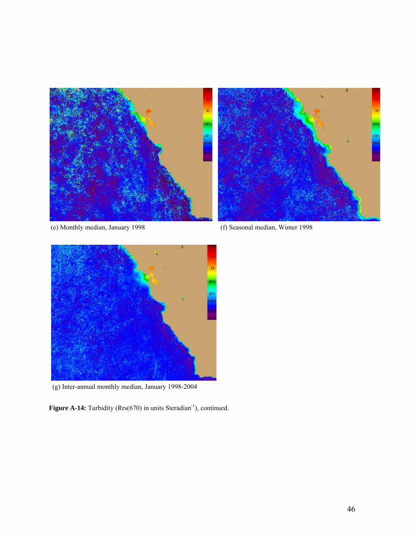
(e) Monthly median, January 1998 (f) Seasonal median, Winter 1998

(g) Inter-annual monthly median, January 1998-2004 Figure A-14: Turbidity (Rrs(670) in units Steradian-1), continued.

46

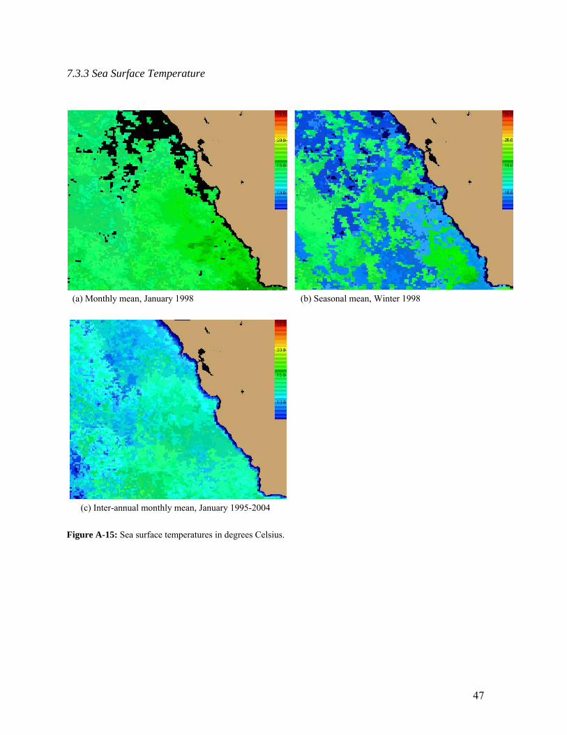
7.3.3 Sea Surface Temperature

(a) Monthly mean, January 1998 (b) Seasonal mean, Winter 1998

(c) Inter-annual monthly mean, January 1995-2004 Figure A-15: Sea surface temperatures in degrees Celsius.

47

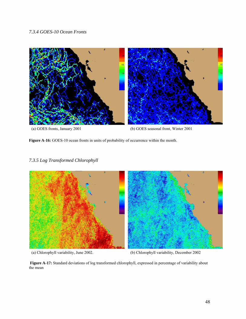
7.3.4 GOES-10 Ocean Fronts

(a) GOES fronts, January 2001 (b) GOES seasonal front, Winter 2001 Figure A-16: GOES-10 ocean fronts in units of probability of occurrence within the month. 7.3.5 Log Transformed Chlorophyll

(a) Chlorophyll variability, June 2002. (b) Chlorophyll variability, December 2002 Figure A-17: Standard deviations of log transformed chlorophyll, expressed in percentage of variability about the mean

48

United States Department of Commerce

Carlos M. Gutierrez Secretary

National Oceanic and Atmospheric Administration

Vice Admiral Conrad C. Lautenbacher, Jr. USN (Ret.) Under Secretary of Commerce for Oceans and Atmospheres

National Ocean Service

Richard W. Spinrad Assistant Administrator for Ocean Service and Coastal Zone Management

Documents

Characterization and Monitoring of Temperature