OULU 1999

CHARACTERIZATION AND APPLICATION OF ANALYSIS METHODS FOR ECG AND TIME INTERVAL VARIABILITY DATA

PAULITIKKANEN

Department of Physical Sciences,Division of Biophysics, and

Biomedical Engineering Program

OULUN YLIOP ISTO, OULU 1999

CHARACTERIZATION AND APPLICATION OF ANALYSIS METHODS FOR ECG AND TIME INTERVAL VARIABILITY DATA

PAULI TIKKANEN

Academic Dissertation to be presented with the assent of the Faculty of Science, University of Oulu, for public discussion in Raahensali (Auditorium L 10), Linnanmaa, on May 24th, 1999, at 12 noon.

Copyright © 1999Oulu University Library, 1999

OULU UNIVERSITY LIBRARYOULU 1999

ALSO AVAILABLE IN PRINTED FORMAT

Manuscript received 30.3.1999Accepted 9.4.1999

Communicated by Professor Metin AkayDocent Kari-Pekka Estola

ISBN 951-42-5214-4(URL: http://herkules.oulu.fi/isbn9514252144/)

ISBN 951-42-5213-6ISSN 0355-3191 (URL: http://herkules.oulu.fi/issn03553191/)

To my family

Tikkanen, Pauli, Characterization and Application of Analysis Methodsfor ECG and Time Interval Variability DataDepartment of Physical Sciences, Division of Biophysics, and Biomedical Engi-neering Program, University of Oulu,FIN-90571, Oulu, Finland.1999Oulu, Finland(Manuscript received 30 March 1999)

Abstract

The quantitation of the variability in cardiovascular signals provides information aboutthe autonomic neural regulation of the heart and the circulatory system. Several factorshave an indirect effect on these signals as well as artifacts and several types of noise arecontained in the recorded signal. The dynamics of RR and QT interval time series havealso been analyzed in order to predict a risk of adverse cardiac events and to diagnosethem.

An ambulatory measurement setting is an important and demanding condition for therecording and analysis of these signals. Sophisticated and robust signal analysis schemesare thus increasingly needed. In this thesis, essential points related to ambulatory dataacquisition and analysis of cardiovascular signals are discussed including the accuracyand reproducibility of the variability measurement. The origin of artifacts in RR intervaltime series is discussed, and consequently their effects and possible correction proceduresare concidered. The time series including intervals differing from a normal sinus rhythmwhich sometimes carry important information, but may not be as such suitable for ananalysis performed by all approaches. A significant variation in the results in either intra-or intersubject analysis is unavoidable and should be kept in mind when interpreting theresults.

In addition to heart rate variability (HRV) measurement using RR intervals, the dy-namics of ventricular repolarization duration (VRD) is considered using the invasivelyobtained action potential duration (APD) and different estimates for a QT interval takenfrom a surface electrocardiogram (ECG). Estimating the low quantity of the VRD vari-ability involves obviously potential errors and more strict requirements. In this study,the accuracy of VRD measurement was improved by a better time resolution obtainedthrough interpolating the ECG. Furthermore, RTmax interval was chosen as the best QTinterval estimate using simulated noise tests. A computer program was developed for thetime interval measurement from ambulatory ECGs.

This thesis reviews the most commonly used analysis methods for cardiovascular vari-ability signals including time and frequency domain approaches. The estimation of thepower spectrum is presented on the approach using an autoregressive model (AR) oftime series, and a method for estimating the powers and the spectra of components isalso presented. Time-frequency and time-variant spectral analysis schemes with applica-tions to HRV analysis are presented. As a novel approach, wavelet and wavelet packettransforms and the theory of signal denoising with several principles for the thresholdselection is examined. The wavelet packet based noise removal approach made use of anoptimized signal decomposition scheme called best tree structure. Wavelet and waveletpacket transforms are further used to test their efficiency in removing simulated noisefrom the ECG. The power spectrum analysis is examined by means of wavelet transforms,which are then applied to estimate the nonstationary RR interval variability. Chaoticmodelling is discussed with important questions related to HRV analysis.

Keywords: Autonomic regulation, heart rate variability, RR interval, ventricularrepolarization duration, ambulatory data, time and frequency domain, wavelettransforms, denoising

Acknowledgements

The research reported in this thesis was carried out in the Division of Biophysicsat the Department of Physical Sciences, University of Oulu, Finland, during theyears 1994-98.

I would like to express my gratitude to Professor Martti Mela for the opportunityto do this work and for his supervision and advice during the course of the study.

I am deeply grateful to Docent Lawrence C. Sellin for patient guidance andsupervision of the research projects. Without his expert support carrying throughthis study would have been much harder and taken longer. I am indebted to himfor effective team-work, help in writing the reports, and revising the language ofthe thesis.

I wish to thank Professor Heikki Huikuri for expert guidance and collaborationregarding the medical aspects of this work.

I would like to thank Professor Matti Weckstrom for the cooperation withinthe last few months spent in finishing the thesis. I would also like to express mygratitude to Professor Rauno Anttila, the former head of the department, for hisuseful collaboration. Stimulating discussions with Professor Matti Karras in thecourse of the work are also greatly appreciated.

I am indebted to Dr. Seppo Nissila and Ilkka Heikkila for their expertise withinthese years. I wish to thank Hannu Kinnunen and Jan-Erik Palmgren for thepleasant teamwork in the subprojects involved in this work. I also appreciatemuch the expert knowledge of Medical Physicist Markku Linnaluoto which wasneeded in the study.

I am grateful to Professor Metin Akay, Darthmouth College, Thayer Schoolof Engineering, USA, and Docent Kari-Pekka Estola, Nokia Research Center,Helsinki, Finland, the official reviewers of the thesis, for their comments and sug-gestions to the manuscript. I would like to thank Docent Tapio Rantala for readingand commenting the manuscript.

The financial support granted by Astra Finland, Instrumentariumin tiedesaatio,Division of Biophysics and Biomedical Engineering Program, University of Oulu isgratefully acknowledged. The computational facilities provided by the Center forScientific Computing, Espoo, Finland, were an important component in performingthe study.

I thank the rest of the staff at the Department of Physical Sciences, especiallyin the Division of Biophysics for help and cooperation within the course of thework.

Finally, I would like to thank my wife Virpi and daughter Venla for their supportand patience during these years. They have given a great deal of welcome changeduring the sometimes lonely work.

Oulu, March 1999 Pauli Tikkanen

List of original papers

This thesis is based on the following papers, which are referred to in the text bytheir Roman numerals:

I Tikkanen P, Kinnunen H, Nissila S, Heikkila I & Mela M (1999) Ambulatoryheart rate variability analysis methods. Automedica 17(4): 237-267.

II Tikkanen PE, Sellin LC, Kinnunen HO & Huikuri HV (1999) Using simulatednoise to define optimal QT intervals for computer analysis of ambulatoryECG. Medical Engineering & Physics 21(1): 15-25.

III Tikkanen PE (1999) Nonlinear wavelet and wavelet packet denoising of ECGsignal. Biological Cybernetics 80(4): 259-267.

IV Huikuri HV, Airaksinen KEJ, Koistinen MJ, Palmgren J-E, Linnaluoto MK,Tikkanen P & Sellin LC (1997) Two-dimensional vector analysis of beat-to-beat dynamics of ventricular repolarization. Annals of Noninvasive Electro-cardiology 2(2): 121-125.

Paper I deals with the data analysis methods for heart rate variability timeseries and discusses also several aspects related to data recorded in ambulatorysettings. The author has been mainly responsible for organizing and writing thetext, only the part dealing with artifacts, their effects and correction was writtenby Hannu Kinnunen, M.Sc. Derivation of the data analysis methods, research anddiscussion on the characterization of the presented methods was performed by theauthor. The examples of data analysis were produced also by the author. Thislong paper could have been published also in two separate papers, but it wasmore convenient to bind these together due to clarity of the presentation. In QTinterval study (paper II) the author was in charge of writing the manuscript, solelyplanned the simulation scheme and performed the data analysis. The computerprogram was developed and written by the author, except the first versions of

the waveform detection algorithms, which were coded by Hannu Kinnunen, M.Sc.,under supervision of the author. Developing signal processing settings e.g. forinterpolation, interpreting and reporting the results were done by the author.Paper III has been produced solely by the author. Therefore, the development ofthe signal analysis schemes, performing the simulations and reporting the resultswere carried out by the author. In paper IV, the author was responsible forthe signal analysis methods in the course of the study. Developing a computerprogram for the analysis of MAP signals was done by Jan-Erik Palmgren, M.Sc.,under supervision of the author. The author was also responsible for the technicalaspects of the paper. The results reported in section 5.4 are not presented in anyof the original papers. Theoretical research linked to that section as well the dataanalysis were completely performed by the author. Further, the thesis includessome theoretical considerations which are not given in the original papers. Thesewere created by the author alone.

Abbreviations

AIC Akaike information criterionAGC Automatic gain controlAMI Acute myocardial infarctionANS Autonomic nervous systemAPD Action potential durationAR AutoregressiveAV AtrioventricularCHF Congestive heart failureCO Cardiac outputCSA Compressed spectral arraysCTM Measure of central tendencyCWT Continuous wavelet transformCV Coefficient of variationDWD Discrete Wigner distributionDWT Discrete wavelet transformECG ElectrocardiogramFIR Finite impulse responseFFT Fast Fourier TransformFHRV Fetal heart rate variabilityFPE Final prediction errorHF High frequencyHR Heart rateHRV Heart rate variabilityLF Low frequencyLF/HF The ratio of the power estimates for the LF and HF componentsLMS Least mean squareMAP Monophasic action potential

MI Myocardial infractionMP Matching pursuitpNN50 The percentage of difference between adjacent normal RR intervals

greater than 50 ms computed over the entire 24 hour ECG recordingQMF Quadrature mirror filterQRS Q-, R-, and S-waves in electrocardiogramQT QT time intervalRLS Recursive least squareRMSSD Root mean square of successive differencesRR RR time intervalRT RT time intervalRWED Running windowed exponential distributionSA SinoatrialSD Standard deviationSDA Selective discrete Fourier transform algorithmSDNNIDX The mean of the standard deviations of all normal RR intervals for

all five minutes segments of a 24 hour ECG recordingSPWD Smoothed pseudo Wigner distributionSTFT Short-time Fourier transformSV Stroke volumeSURE Stein’s unbiased risk estimateTFR Time frequency representationTI NN Triangular interpolation of the normal-to-normal histogramULF Ultra low frequencyWD Wigner distributionWP Wavelet packetWT Wavelet transformVLF Very low frequencyVRD Ventricular repolarization duration

Contents

AbstractAcknowledgementsList of original papersAbbreviationsContents1. Introduction . . . . . . . . . . . . . . . . . . . . . . . . . . . . . . . . . . 15

1.1. Background . . . . . . . . . . . . . . . . . . . . . . . . . . . . . . . 151.2. Aims and the outline of the thesis . . . . . . . . . . . . . . . . . . 17

2. Cardiovascular variability signals . . . . . . . . . . . . . . . . . . . . . . 182.1. Physiological background . . . . . . . . . . . . . . . . . . . . . . . 182.2. Changes of signal variability connected to specific diseases . . . . . 202.3. Other events modifying signal variability . . . . . . . . . . . . . . . 212.4. RR interval time series . . . . . . . . . . . . . . . . . . . . . . . . . 212.5. VRD time series . . . . . . . . . . . . . . . . . . . . . . . . . . . . 222.6. APD time series . . . . . . . . . . . . . . . . . . . . . . . . . . . . 232.7. ECG waveform detection . . . . . . . . . . . . . . . . . . . . . . . 232.8. Ambulatory HRV data . . . . . . . . . . . . . . . . . . . . . . . . . 25

2.8.1. Accuracy of HRV measurement . . . . . . . . . . . . . . . . 252.8.2. Reproducibility of HRV measurements . . . . . . . . . . . . 262.8.3. Artifacts in RR interval time series . . . . . . . . . . . . . . 27

2.8.3.1. Errors in the detection and classification of QRScomplexes . . . . . . . . . . . . . . . . . . . . . . . 27

2.8.3.2. Non-periodic changes in RR intervals . . . . . . . 302.8.4. Limitations and effects of artifacts . . . . . . . . . . . . . . 312.8.5. Correction of abnormal RR intervals . . . . . . . . . . . . . 32

2.8.5.1. Detection of artifacts . . . . . . . . . . . . . . . . 332.8.5.2. Correction of artifacts . . . . . . . . . . . . . . . . 34

3. Analysis of signal variability . . . . . . . . . . . . . . . . . . . . . . . . . 353.1. Interpolation of the ECG signal . . . . . . . . . . . . . . . . . . . . 353.2. Time domain analysis . . . . . . . . . . . . . . . . . . . . . . . . . 36

3.2.1. Time domain indices . . . . . . . . . . . . . . . . . . . . . . 363.2.2. Analysis of distribution . . . . . . . . . . . . . . . . . . . . 37

3.3. Frequency domain analysis . . . . . . . . . . . . . . . . . . . . . . 383.3.1. Interpretation of spectral estimates . . . . . . . . . . . . . . 383.3.2. On the use of spectral analysis . . . . . . . . . . . . . . . . 393.3.3. Mathematical background to spectral analysis . . . . . . . . 403.3.4. Spectrum estimation using a periodogram . . . . . . . . . . 413.3.5. Parametric modelling of time series . . . . . . . . . . . . . . 42

3.3.5.1. AR spectrum estimate . . . . . . . . . . . . . . . . 433.3.5.2. Estimation of the powers related to components . 443.3.5.3. Model order selection . . . . . . . . . . . . . . . . 45

3.3.6. Bispectrum estimation . . . . . . . . . . . . . . . . . . . . . 453.4. Time frequency analysis . . . . . . . . . . . . . . . . . . . . . . . . 46

3.4.1. Time frequency representations . . . . . . . . . . . . . . . . 463.4.2. Time-variant spectral analysis . . . . . . . . . . . . . . . . . 46

3.5. Wavelet analysis . . . . . . . . . . . . . . . . . . . . . . . . . . . . 483.5.1. Continuous wavelet transform . . . . . . . . . . . . . . . . . 483.5.2. Discrete wavelet transform . . . . . . . . . . . . . . . . . . 503.5.3. Multiresolution wavelet analysis . . . . . . . . . . . . . . . 503.5.4. Subband filtering . . . . . . . . . . . . . . . . . . . . . . . . 513.5.5. Wavelet packet analysis . . . . . . . . . . . . . . . . . . . . 523.5.6. Optimization of the wavelet packet decomposition . . . . . 533.5.7. “De-noising” the signal . . . . . . . . . . . . . . . . . . . . 543.5.8. Selection of the threshold . . . . . . . . . . . . . . . . . . . 55

3.6. Chaotic modelling . . . . . . . . . . . . . . . . . . . . . . . . . . . 564. Experimental settings . . . . . . . . . . . . . . . . . . . . . . . . . . . . 59

4.1. RR interval data . . . . . . . . . . . . . . . . . . . . . . . . . . . . 594.2. Dynamics of the ventricular repolarization duration . . . . . . . . . 59

4.2.1. Measurement equipment and software . . . . . . . . . . . . 594.2.2. Testing of the automatic waveform measurement . . . . . . 60

4.2.2.1. Real ECG signals . . . . . . . . . . . . . . . . . . 604.2.2.2. Simulated ECG signals . . . . . . . . . . . . . . . 60

4.3. Denoising of an ECG signal . . . . . . . . . . . . . . . . . . . . . . 624.4. Analysis of APD time series . . . . . . . . . . . . . . . . . . . . . . 62

4.4.1. Patients . . . . . . . . . . . . . . . . . . . . . . . . . . . . . 624.4.2. Study protocol . . . . . . . . . . . . . . . . . . . . . . . . . 634.4.3. Analysis of MAP signals . . . . . . . . . . . . . . . . . . . . 644.4.4. Analyses of variability of RR intervals and action potential

duration . . . . . . . . . . . . . . . . . . . . . . . . . . . . . 644.5. Wavelet analysis of HRV . . . . . . . . . . . . . . . . . . . . . . . . 65

5. Results . . . . . . . . . . . . . . . . . . . . . . . . . . . . . . . . . . . . 665.1. Dynamics of the ventricular repolarization duration . . . . . . . . . 66

5.1.1. Interpolation of the ECG . . . . . . . . . . . . . . . . . . . 665.1.2. RMSSD of QT interval time series . . . . . . . . . . . . . . 665.1.3. Power spectrum estimates . . . . . . . . . . . . . . . . . . . 685.1.4. Simulated ECG signals . . . . . . . . . . . . . . . . . . . . 715.1.5. Discussion . . . . . . . . . . . . . . . . . . . . . . . . . . . . 72

5.2. Wavelet transform based noise removal of ECG . . . . . . . . . . . 75

5.2.1. Overall performances . . . . . . . . . . . . . . . . . . . . . . 765.2.2. Performances within QRS-complex . . . . . . . . . . . . . . 775.2.3. Checking the error signals . . . . . . . . . . . . . . . . . . . 785.2.4. Discussion . . . . . . . . . . . . . . . . . . . . . . . . . . . . 79

5.3. Analysis of APD variability . . . . . . . . . . . . . . . . . . . . . . 825.3.1. Discussion . . . . . . . . . . . . . . . . . . . . . . . . . . . . 83

5.4. Spectral estimation using wavelet transforms . . . . . . . . . . . . 845.4.1. Discussion . . . . . . . . . . . . . . . . . . . . . . . . . . . . 85

6. Summary and conclusion . . . . . . . . . . . . . . . . . . . . . . . . . . 90References . . . . . . . . . . . . . . . . . . . . . . . . . . . . . . . . . . . . . 94Original papers

1. Introduction

1.1. Background

Variabilities in cardiovascular activity, such as RR interval and ventricular repo-larization duration (VRD), have been widely used as a measure of cardiovascularfunction. It is typical for these signals that they fluctuate on a beat-to-beat basisaround their mean value and the fluctuation are associated with autonomic neuralregulation of the heart. Monitoring the fluctuations observed in heart rate andVRD thus provides information concerning their autonomic regulation and distur-bances. For example, heart rate fluctuates due to factors such as age, respiration,cardiovascular and neurologic diseases, medication, as well as physical and mentalstress (Malliani et al. 1991, VanRavenswaaij-Arts et al. 1993, Pagani et al. 1995).

To predict a risk of adverse cardiac events the primary analytical measurementshave been heart rate variability (Moser et al. 1994, Tsuji et al. 1994) and QT anal-ysis (Decker et al. 1994). Abnormalities in heart rate fluctuation have been shownto precede the spontaneous onset of ventricular tachyarrhythmias (Huikuri et al.1996). For example, low heart rate variability predicts increased mortality afteracute myocardial infarction (AMI) (Malik et al. 1990). Clinical and experimentaldata have shown that prolongation of the QT interval measured from the stan-dard 12-lead ECG is a risk factor for ventricular arrhythmia and sudden cardiacdeath in patients with or without previous AMI. The increased risk due to QTprolongation is independent of age, history of AMI, heart rate and drug use. Thevariability of successive RR intervals traditionally has been used to access the riskin patients in terms of future mortality. Recently, emphasis has been directed to-wards understanding the dynamic changes in the repolarization phase of the heart(Extramiana et al. 1997, Huikuri 1997). It is probable that there are dynamicchanges in the ventricular repolarization duration (QT interval) throughout the24-hour period (Merri et al. 1993).

The autonomic nervous system (ANS) regulates the functioning of the heartthrough its sympathetic and parasympathetic parts. It is of interest to quantifythe amounts of signal fluctuation related to these two parts of the ANS separatelyand also their balance in the neural regulation of the heart. For instance, heart

16

rate is affected by factors such as respiration, the thermoregulatory system andmechanisms regulating blood pressure (Hainsworth 1995).

Autonomic regulation of the heart and the cardiovascular system has been in-vestigated widely, but no uniform concept exists regarding the function of neuralmechanisms. Furthermore, there is a lack of standardization of the parametersand their meaning in signal variability analysis. For example, the analysis of thefrequency spectrum is made using several approaches such as Fourier transformand AR-modelling based methods with several variations.

The quantification of neural regulation is a demanding task, because interpreta-tion relies on an indirect measurement, i.e. the observed fluctuation in cardiovas-cular variability signals. The heart rate signal includes noise from various sourcesand information not related to autonomic regulation of the heart summed withthe relevant information. There are technical and methodological limitations inthe measurement of the QT interval, for example, due to artifacts, low samplingfrequency, and inaccuracies in the definition of the end of the T wave in the am-bulatory ECG recordings. Measurement of monophasic action potential (MAP)with a contact electrode have been confirmed as an accurate method for analysisof local ventricular repolarization duration (Franz 1991).

Heart rate variability (HRV) has been studied extensively during the last fewyears. The analysis of the frequency spectrum of the heart rate signal has at-tracted attention mainly due to its ability to expose different sources of fluctua-tions (Baselli et al. 1987, Bianchi et al. 1993, Kamath & Fallen 1993, Malliani et al.1991) and its power to illustrate the balance of the autonomic neural regulation.There also exist several widely used time-domain parameters representing fluctu-ations in heart rate (Kleiger et al. 1992). Lately, more emphasis has been placedon the non-linear analysis of heart rate variability (Huikuri et al. 1996, Signoriniet al. 1994).

The analysis of variability in cardiovascular signals is applied widely and thereare thus many differences in experimental setups. In addition, the parameters usedfor quantifying variability vary from one area of research to another. The meaningof some parameters may remain unclear, and the understanding of the applicationsof novel methods can also be imperfect. Sometimes, these factors can make itrelatively difficult to interpret the results and compare them among the projects.Data are commonly recorded in a laboratory, where the conditions are strictlycontrolled and the effects of disturbing factors are minimized. The recording ofambulatory data is affected by many outside disturbances, and therefore, specialinterest must be taken in the quality of the recorded data and the characteristicsof the analytical methods. Neglect of such matters can lead to serious errors ininterpreting the results.

17

1.2. Aims and the outline of the thesis

This study is a methodological approach to deal with the analysis of short termfluctuations in the cardiovascular variability signals. In this context, the periodsof the oscillations observed in signals vary from a few seconds to tens of seconds.

The thesis includes the development of analysis schemes and studies of thedynamics of RR interval, ventricular repolarization duration (VRD) and actionpotential duration (APD) time series. Some emphasis will be on the ambulatorydata with discussion of the accuracy and the reproducibility of the measurementas well as the effects of artifacts. A computer program for the measurement ofRR and QT intervals from the ambulatory electrocardiogram (ECG) is described.Furthermore, the accuracy of the different QT interval estimates will be obtainedthrough simulated noise tests. The invasive measurement of APD variability isused to emphasize the requirements needed for the VRD variability estimationand to study the factors determining the VRD dynamics. The novel wavelettransform approaches are proposed to remove noise from ECG and the denoisingperformances are quantified by simulations. The spectral estimation using wavelettransforms will be presented for RR interval data obtained from healthy subjectsduring a drug injection and from ordinary cardiology patients prior to the onsetof ventricular fibrillation. Overall, the stress is more on the demonstration of thesignal analysis schemes than the larger data analysis settings.

A review of the signal analysis methods applied to cardiovascular variabilitysignals is provided. Furthermore, the limits and advantages of the methods arediscussed. An important point is to present the mathematical background ofthe methods and demonstrate their application using some experimental data.It is worth noting that there often exist a correlation between the results andsome phenomena, but the analysis method may not be a suitable one to describethese phenomena. To obtain relevant results and a correct diagnosis, a deeperunderstanding of the nature of applied methods would be necessary. There areoften some basic assumptions and rules for the methods and signals, which shouldbe taken account in order to make the analysis more useful. As the evaluation ofthe results is made with deeper understanding of the methodological aspects, onecan better say “what is actually possible to show by our results”.

First the physiological and medical background is briefly reviewed in order togive some basis for the application of the analytical methods. Extraction of the car-diovascular variability signals is presented and important aspects of measurementtechniques are pointed out. The mathematical and methodological backgroundis presented for time and frequency domain analysis methods. The estimation ofthe power spectrum is considered important especially the parametric methodsand the autoregressive (AR) approach. Time-frequency and time-variant spectralanalysis methods are reviewed and a novel wavelet approach is introduced. Thewavelet section includes discussions of the continuous and discrete wavelet trans-form with a subband filtering scheme as well as a more recent application of thewavelet packet transform using an optimized signal decomposition. The use ofchaotic modelling is also considered and important issues related to HRV analysesare presented.

2. Cardiovascular variability signals

2.1. Physiological background

The sinus rhythm fluctuates around the mean heart rate, which is due to continu-ous alteration in the autonomic neural regulation, i.e. sympathetic-parasympatheticbalance. Periodic fluctuations found in heart rate originate from regulation relatedto respiration, blood pressure (baroreflex) and thermoregulation.

Parasympathetic (vagal) regulation to the heart is inhibited simultaneously withinspiration, and the breathing frequency coincides with fluctuations observed inheart rate (Eckberg 1983). Furthermore, thoracic stretch receptors and periph-eral hemodynamic reflexes also result in respiratory arrhythmia (Akselrod et al.1985). Respiratory arrhythmia are consequently due to parasympathetic regula-tion and can be excluded by atropine or vagotomy (Akselrod et al. 1985). Themaximal amplitude of respiratory related heart rate fluctuation is found at breath-ing rate of 6 cycles per minute, because the fluctuation increases as respiration rateachieves the frequency of the intrinsic baroreflex-related heart rate fluctuations(VanRavenswaaij-Arts et al. 1993).

The fluctuations due to blood pressure regulating mechanisms originate fromself-oscillation in the vasomotor part of the baroreflex loop (VanRavenswaaij-Artset al. 1993). These fluctuations coincide with synchronous oscillations in bloodpressure called Meyer waves (Kitney & Rompelman 1987). Increase of sympa-thetic nerve impulses strengthen (Pagani et al. 1984, Pomeranz et al. 1985) andsympathetic or parasymphatetic blockade weaken these fluctuations in heart rate(Pomeranz et al. 1985).

Changes in peripheral resistance produce low frequency oscillations in heartrate and, for example, in systolic blood pressure. Thermal stimulation given onthe skin can be used to stimulate the oscillations, which are originally due tothermoregulatory adjustment of peripheral blood flow (VanRavenswaaij-Arts et al.1993). These fluctuations are controlled by the sympathetic part of the autonomicnervous system.

The overall autonomic function is controlled by a central command from thebrain. However, the autonomic nervous system operates as a feedback system, andheart rate is thus regulated by many reflexes which may increase or decrease the

19

sympathetic or parasympathetic activity or both of them (Hainsworth 1995). Re-flexes can act simultaneously and their interactions may be complex. The arterialbaroreceptor reflex originates from receptors located in the arteries such as carotidsinuses and aortic arch. The increase in blood pressure excites baroreceptors pro-ducing an augmented efferent vagal and reduced sympathetic activity. Peripheralarterial chemoreceptors located in the carotid and aortic bodies produce, mostoften, an increase in the rate and depth of respiration. Because this reflex in-fluence on heart rate through respiration, the effects may be covered by otherrespiratory responses. The coronary chemoreflex (Bezold-Jarisch reflex) can causebradycardia and is significant in pathological states such as myocardial ischemiaand infarction. Atrial receptors streched by the increase in atrial volume and someof them by atrial contraction, the response being linked directly to atrial pressure.These volume receptors cause an increase in heart rate and operate through thesympathetic nerves producing their response very slowly. There exist also othercardiovascular reflexes coming from receptors located e.g. in pulmonary arteries,lungs and muscles.

The physiological importance of heart rate can be demonstrated by an axiomaticrelation in which cardiac output (CO) can be defined by a product between heartrate and stroke volume (SV) as CO = HR · SV. Because heart rate and strokevolume are not independent of each other, the definition of cardiac output is notalways so straightforward in terms of physiological adjustment.

The rate of depolarization of the cardiac pacemaker defines heart rate. Thesinoatrial (SA) node, the atrioventricular (AV) node and the Purkinje tissue canbe regarded as potential pacemaker tissues in a heart. As the fastest depolariza-tion rate is found in the sinoatrial node and the depolarization impulse spreadsthrough the conduction system to other pacemakers before they spontaneouslydepolarize, the sinoatrial node usually defines the heart rate. However, failing toproduce a normal pacemaker impulse, other pacemaker tissues can act as a cardiacpacemaker.

Autonomic neural regulation of the heart is determined by its sympathetic andparasympathetic parts. The parasympathetic nerves are connected to the sinoa-trial node, the AV conducting pathways and the atrial and ventricular musclesas well as coronary vessels (Kamath & Fallen 1993). Sympathetic nerve fibersinnervate the SA node, the AV conducting pathways, coronary vessels and theatrial and ventricular myocardium (Kamath & Fallen 1993, Hainsworth 1995).Both divisions of the autonomic nervous system always have some activity whichcontinuously regulates the function of the heart. Heart rate response thereforepresents a balance between sympathetic and parasympathetic (vagal) regulationwhich can be considered also as an antagonist function.

Heart rate has a major effect on ventricular repolarization duration (VRD),but the autonomic nervous system also regulates directly the repolarization of theventricles. In addition, electrolytic factors, age and gender have an effect on it.It has been shown that when the autonomic nervous system regulates VRD thereare similar periodic fluctuations as seen in heart rate (Merri et al. 1993).

20

2.2. Changes of signal variability connected to specificdiseases

A decrease in vagal neural activity into the heart may result in diminished HRVafter myocardial infarct (MI) leading to the prevalence of symphatetic neural reg-ulation and to electrical instability (Task Force of ESC & NASPE 1996). Reducedheart rate variability is also associated with an increased risk for ventricular fibril-lation and sudden cardiac death (Farrell et al. 1991, Casolo et al. 1992). Huikuriet al. (1996) concluded that changes in long term RR interval dynamics with beat-to-beat RR interval alternans is likely to precede the spontaneuous onset of sus-tained ventricular tachyarrhythmias. Results obtained using spectral analysis ofHRV suggest a change of sympatho-vagal balance toward a symphatetic dominanceand a diminished vagal tone in patients surviving an acute myocardial infarction(Lombardi et al. 1992, Task Force of ESC & NASPE 1996). Cardiac diseasessuch as congestive heart failure, coronary artery disease and essential hyperten-sion are also associated with a reduced vagal and an enhanced sympathetic tone,which change heart rate varibility dynamics (VanRavenswaaij-Arts et al. 1993,Malliani et al. 1991). Because HRV analysis can be regarded as a noninvasive,reproducible and an easy to use method reflecting the degree of autonomic controlof the heart (Bellavere 1995), it has been widely used to diagnose the autonomicdysfunction due to diabetic neuropathy (Pagani et al. 1988a, Freeman et al. 1991,Bernardi et al. 1992). It has been generally observed, that overall HRV is reducedand sympatho-vagal balance may be altered during tilt maneuver or standing indiabetic patients (Malliani et al. 1991, Kamath & Fallen 1993).

Although HRV is used in a wide range of clinical applications, diminished HRVhas only been generally accepted as a predictor of risk after acute myocardialinfarction and as an early warning of diabetic neuropathy. Diminished HRV canpredict mortality and arrhythmic events independently of other risk factors afteracute myocardial infaction, and long-term HRV analysis have proven to be a moredefinite predictor compared to a short-term analysis (Task Force of ESC & NASPE1996). Heart rate variability analysis should also be joined with other risk factorsso as to improve the predictive use.

Any heart disease (left ventricular hyperthrophy, heart failure, etc.) can modifyrepolarization duration (Coumel et al. 1994). Anomalies in repolarization durationare signs of electrical instability in the heart and can lead to malignant arrhythmiassuch as ventricular fibrillation and Torsades de Pointes. Analysis of ventricularrepolarization duration dynamics provides essential information on a propensityfor ventricular arrhythmias, because some life-threatening arrhythmias arise inmyocardial tissue (Huikuri 1997). Altered dynamics of the VRD, and the eventsof the alternating T wave amplitude particularly in patients with the long QTsyndrome as well as with structural heart disease at fast heart rates, suggest thatthe analysis of the ventricular repolarization dynamics may provide an importantclinical tool (Huikuri 1997).

21

2.3. Other events modifying signal variability

Several pharmaceutical interventions can be used to modify heart rate dynamics asshown by human (Selman et al. 1982) and animal (Adamson et al. 1994) studies.Atropine administration has been used to prove the connection between vagalneural activity and high frequency (respiratory related) fluctuation in RR intervaltime series (Pomeranz et al. 1985). Scopolamine significantly augments heart ratevariability (Ferrari et al. 1993) which suggest an increasing coincident vagal activityinto the heart. The effect of β-adrenergic receptor blockades has been studied aftermyocardial infarction (Molgaard et al. 1993, Sandrone et al. 1994). There are alsostudies on the effect of antiarrhythmic drugs such as flecainide (Zuanetti et al.1991, Bigger et al. 1994) and propafenone (Zuanetti et al. 1991, Lombardi et al.1992), as well as encainide and moricizine (Bigger et al. 1994) on the heart ratedynamics. Merri et al. (1993) studied the effect of β-adrenergic blocker (nadolol)on ventricular repolarization duration and its dynamics. Their finding was thatthe length of repolarization duration was shorter, the signal variance was greaterand the spectral pattern was shifted to higher frequencies due to this medication.A change of the dynamic relationship between ventricular repolarization durationand heart rate has been observed as a consequence of nadolol administration withnormal patients (Merri et al. 1992).

Heart rate variability has been employed to investigate the short and long termautonomic responses to physical and mental exercise. It has been observed thatthe increase in respiratory related fluctuation, the total HRV reduction and therecorded signal become more nonstationary as the intensity of the dynamic physicalexercise increases (Malliani et al. 1991). Heavy physical exercise has been shownto augment low-frequency (LF) fluctuations in heart rate, and the recovery of thespectral pattern may last even 48 hours after finishing exercise (Furlan et al. 1993).The sympatho-vagal balance seems to change towards sympathetic dominance e.g.in hypertensive patients (Pagani et al. 1988b). Long term physical exercise haspositive effects on hemodynamics and neural control mechanisms, for example, bylowering the arterial pressure in hypertensive patients (Pagani et al. 1988b) andincreasing baroreflex gain in patients with ischemic heart disease (Rovere et al.1988). An overall observation, also related to dynamic mental stress, is an increaseof the sympathetically- and a decrease of vagally-mediated fluctuations in heartrate (Pagani et al. 1995).

2.4. RR interval time series

The basic procedure used for determing the heart rate and its fluctuations isdescribed below. An electrocardiogram (ECG) is measured, using appropriatedata acquisition equipment. The time elapsing between consecutive heart beats isdefined as that between two P waves, when a P wave describes the phase of atrialdepolarization. In practice, it is the QRS complex that is used to obtain the timeperiod between heart beats. This complex is detected in the R wave, because it

22

has a very clear amplitude and better frequency resolution than the P wave, anda much better signal-to-noise ratio. The time interval between the P and R wavescan be assumed and has been shown to be constant (Kitney & Rompelman 1987).

Defining the times of occurrence of two concecutive R waves as s(t) and s(t+1),t = 1, . . . , N , the expression x(t) = s(t + 1) − s(t) is obtained for a time periodin milliseconds. This x(t) is called the RR interval time series or else the timesto which it refers are simply called RR intervals. A heart rate time series [min−1]can be obtained by y(t) = 1000 · (60/x(t)) and the mean heart rate is simplyHR = N−1

∑Nt=1 y(t). These formulae indicate a nonlinear relationship between

the values in a given time series, which should be taken into account when com-paring the results obtained by time and frequency domain approaches (Sapoznikovet al. 1993). At the moment, RR intervals seem to be the more frequently usedtime series in heart rate variability (HRV) analysis. For a discussion of the choicebetween different time series (tachograms), see Janssen et al. (1993).

2.5. VRD time series

QT time interval in electrocardiographic signals has been used to perform bothstatic and dynamic analyses of the duration of the ventricular repolarization.There exist difficulties in the detection of the onset of Q wave and the offset of Twave due to poor signal-to-noise ratio and varying ECG morphology. For these rea-sons other estimates, such as RTmax interval, has been widely used. Moreover, thisprovided a motivation to investigate and compare the noise sensitivity of differentQT interval estimates. Because Q-S time interval is a result of the depolarizationperiod of the ventricles, it is actually more correct to measure the time intervalbetween the R and T waves as one is interested in the changes occurring withinthe ventricular repolarization period (Merri et al. 1989). R wave has been used toestimate the start of the repolarization period because searching for the offset of Swave can be difficult. The maximum (apex) of T wave has been often regarded asa more reliable estimate for the end of the repolarization period than the T waveoffset. The total repolarization duration, i.e. time interval between the offsets of Sand T waves, can further be analysed with respect to early and late repolarizationduration as well as repolarization area (Merri et al. 1989, Merri 1989). In thiswork the objective will be on the measurement of the repolarization duration inthe ambulatory ECG.

The 24-hour ambulatory ECG has certain problems and drawbacks because thesignal is corrupted by noise from various sources and also several conditions mayalter the ECG morphology. The ambulatory ECG is usually acquired with a sam-pling frequency of 128 Hz giving a time resolution of 7.81 ms for each sample,which is too low for QT interval variability measurement. It has been suggestedthat the QT interval should be determined at least with resolution of 1 ms (Sper-anza et al. 1993), which would require 1 kHz sampling frequency for ECG signal.In an ambulatory measurement setting, with data acquisition times lasting up to24 hours, the sampling frequency can not be that high, because then the amount

23

of the stored data rises rapidly. In present ambulatory ECG analysis systems thepossibility of exporting a beat-to-beat QT time series extracted with high time res-olution is also lacking. These problems have been solved by exporting raw ECGdata and, by oversampling ECG signal (Speranza et al. 1993) or by interpolat-ing waveforms (Merri et al. 1991) a better time resolution for the time intervalmeasurement results.

2.6. APD time series

The local ventricular repolarization duration can be measured by placing a con-tact electrode in a ventricular muscle. Rate-dependent dynamics of VRD obtainedfrom the right ventricular apex provides an example. This approach can solve theabove mentioned problems related to the ambulatory QT measurement. However,measuring monophasic action potentials (MAP) is an invasive procedure. The du-ration of repolarization phase, which is termed as action potential duration (APD),is estimated as a time interval between the onset and offset of the action potential.The offset is defined as the maximal positive derivative of the upstroke phase ofthe action potential waveform. The offset can be defined at time points wherethe waveform has come down 15, 30, 50 and 90 % from the maximal amplitudeof the MAP. Most often used definitions are 50 and 90 % points. The APD timeseries are extracted from the consecutive waveforms and the beat-to-beat analysisis performed.

2.7. ECG waveform detection

The RR and QT interval measurement (paper II) was based on an implementationof an algorithm described previously (Laguna et al. 1990) and the detection schemewill be briefly reviewed here. The basic concept of the algorithm is to look for thezero crossing points, the crossings of certain experimentaly-determined thresholdvalues, as well as the local maximum or minimum values of the differentiated ECGsignal d(t) and its low-pass filtered version f(t).

The differentiator and the low-pass filter described by Laguna et al. (1990) weremodified according to the sampling rate in order to obtain an optimal frequencyresponse. The sampling rate of the analysed ECG was one parameter of thewaveform detection procedure, and in this way, the preprocessing filters and thealgorithm itself can adapt to the different sampling rates.

The flowchart of the implemented waveform detection procedure is shown inFigure 1 in paper II. The first step is to calculate the signals d(t) and f(t), whichis done for the whole period of the ECG selected for analysis. The waveformdetection procedure continues by determining the initial value of the thresholdvalue Hn used to search the maximum absolute value of the QRS in the signalf(t). The threshold value Hn+1 is continuously updated (Laguna et al. 1990)

24

during the waveform detection using the equation

Hn+1 = 0.8 ·Hn + (0.16 · |f(PKn)|) , (2.1)

where |f(PKn)| is the absolute value of the signal f(t) at the detected fiducial Rwave position of the beat n.

The initialisation of the average of RR intervals RRav and the first RR intervalvalue are then obtained. The RRav value is later used to check the calculated valueof a new RR interval and thus provides a basis for identifying the QRS complex.

The initial position of a QRS complex is detected using an adaptive thresholdmethod determined by the RR interval average value, as shown in Figure 1 inpaper II. After that, the algorithm continues to search the position of the R wave.In the present approach, the fiducial point of the R wave was detected using threemethods: at the maximum amplitude upwards or downwards from the baseline,or at the zero crossing point of the signal f(t) during the QRS complex. The lasttechnique was implemented in the original algorithm by Laguna et al. (1990). Itwas found that, in some cases, a more accurate definition can be obtained, if thefiducial point of the R wave is defined at the maximal upward amplitude of QRS.With this algorithm, an accurate determination of the R wave is an absolutelynecessary condition for a reliable Q wave detection.

After detecting the R wave position and updating the threshold Hn and RRav,the onset of Q wave is searched keeping the R wave position as a reference point.Here it should be mentioned, that examining the pattern of the Q wave is made byanalysing the differentiated signal d(t) and not the signal f(t), because the signald(t) includes the high frequency components of the Q wave.

Next the T wave maximum and T wave end are detected from the signal f(t).The following definition for the limits of a search window calculated from the Rwave position was used:

(bwind, ewind) = (a · RRav, b ·RRav) , (2.2)

where a and b are parameter values in the procedure. This definition is a slightlydifferent one from the given by Laguna et al. As the threshold for T wave end wasused the value Hs = f(Ti)/2, Ti denoting the position of the maximal downwardor upward slope after the T wave maximum.

Finally, a value of QT interval is calculated using the relationQT (n) = Tend(n)−QTonset(n), where Tend(n) and QTonset(n) are the positions of T wave end and theonset of the QT time interval during the beat n. The analysis of the next cardiacbeat is started 150 ms after the last T wave end is defined.

The effects of the four alternative definitions of the QT interval onset on theanalysis of QT interval dynamics were compared: true QRS onset, R wave maxi-mum, ascending or descending maximal slopes of the R wave. One reason for thiswas quite practical: in some circumstances dealing with ambulatory ECG, thedetermination of the QRS onset seems to be uncertain e.g. because of a missing Qwave and the relatively low sampling rate. In the original implementation of thisalgorithm, the Q wave onset found is rejected if the difference between Q waveand R wave fiducial points is larger than 80 ms (Laguna et al. 1990). In that case,QRS onset is defined in the onset of R wave.

25

2.8. Ambulatory HRV data

The aim of recording RR intervals has been to gain information about the neuralregulation of the heart and the circulatory system. Observing the changes occur-ing over long periods of time (i.e. several hours) requires ambulatory recording,which is usually performed using standard commercial equipment (Holter devices).This provides procedures for ECG signal acquisition and analysis, extracting theRR interval time series from the ECG signal and analysing them. The samplingfrequency typically used for an ECG signal with Holter devices is 128 Hz, whichmeans a timing accuracy of 7.81 ms for R wave detection. Thus a low samplingfrequency produces inaccuracies in RR interval measurement and bias in the anal-ysis. A timing accuracy of the order of 1 ms would be desirable for the assessmentof chaos, for example.

One factor affecting ambulatory HRV measurement is circumstances that varywith time, i.e. the fact that external conditions can be far from stable. This mayproduce nonstationary changes in a time series and make the assessment of thephysiological events more difficult, or even impossible, than under stable laboratoryconditions. A method for separating non-periodic (nonstationary) changes fromperiodic ones has been proposed by Sapoznikov et al. (1994). Variable conditionsmay also produce periodic fluctuations which become summed in the time series,making it difficult to distinguish the regulatory processes from each other. Thiscan obviously lead to misinterpretations in some circumstances.

2.8.1. Accuracy of HRV measurement

The accuracy of spectral estimates performed on RR intervals obtained from am-bulatory Holter systems has been studied by Pinna et al. (1994). It has beenobserved that the centre and dispersion of the estimation error changes from oneHolter system to another. There are large inter-recorder differences and variablespectral distortion among selected spectral bands. Use of the Fourier spectral es-timate gave more stable results than did the AR spectral estimate in ten minuteECG sequences. The main factor limiting the accuracy of the RR interval mea-surement was the low frequency with which the ECG signal was sampled, a topicdiscussed theoretically by Merri et al. (1990). Pinna et al. (1994) concluded thatspectral analysis of RR interval time series with very low variability may be seri-ously altered when performed on an ECG signal acquired using a Holter system.

The accuracy of spectral estimates of HRV was investigated by generating asimulated RR interval time series of variable length (180-540 seconds) using anautoregressive model from a set of recordings and adding Gaussian noise (Pinnaet al. 1996). The accuracy of Fourier (Blackman-Tukey) and AR spectral estimatescould then be evaluated in terms of the normalized bias and variance. The resultsshowed that the bias (systematic error) of the estimate was a less important factorthan the variance (random error). Both decreased as the length of the time seriesincreased, but the variance decreased more rapidly. The power estimate was most

26

stable in the HF band, while that in the VLF band had the highest variance.No minimum length was proposed for a time series, but it was concluded thateven with the shortest record the bias made a less significant contribution to theestimates. It was pointed out that a relative high variability in spectral parametersis typical of RR interval time series, and that this should be noted in the analysisof the short time series.

2.8.2. Reproducibility of HRV measurements

There are a number of factors that affect HRV measurements, and obtaining pre-cisely controlled conditions is problematic. Furthermore, variability is always seenbetween repeated measurements. From this point of view, it is essential to studyboth short-term (over several days or couple of weeks) and long-term (over 6-7months) reproducibility of the analyses, even though this can be a tedious task.A few published investigations on the reproducibility of HRV exist, e.g. referencesDimier-David et al. (1994), Kamalesh et al. (1995), Pitzalis et al. (1996), Pomeranzet al. (1985) and Ziegler et al. (1992).

Kamalesh et al. (1995) investigated the short-term reproducibility of HRV mea-surements in patients with chronic stable angina and found no significant changesin the time or frequency domain parameters between two 24 hour ambulatory ECGrecordings. The short-term and mid-term (over one month) stability of spectralparameters was studied in healthy young subjects by Dimier-David et al. (1994),who observed that the intra-observer and inter-observer reproducibility of spectralanalyses are high under controlled conditions. They did not employ any standard-ization for breathing frequency or volume.

Pitzalis et al. (1996) studied the short and long-term reproducibility of HRVmeasurements in normal subjects. They concluded that time domain parameters,as evaluated over the whole 24 hour recording, can be expected to be reproducibleduring relatively stable conditions but frequency domain parameters calculatedfor ten minute ECG sequences were reproducible only under known stable condi-tions, as factors of other than neural origin can greatly alter the spectrum. Themeasurement of total power needed resting conditions to produce reproducible re-sults. Respiratory oscillations in the spectrum (high frequency component) can bemeasured reproducibly during controlled breathing. The low frequency componentwas reproducible, particularly at rest and during tilt, which indicates that thesefluctuations are quite stable. The reproducibility of the power estimates whennormalized by reference to the total power seemed to be no better than that ofthe real values. It should be noted that the time domain parameters were not re-producible if they were evaluated from ten minutes sequences instead of the whole24 hour period.

The results of analyses performed on signals of short (e.g. five to ten minutes)and long (possibly 24 hours) duration seem to differ. Pitzalis et al. (1996) suggestthat analyses of long signals may homogenize the results and give better repro-ducibility of the frequency domain parameters. In analyses performed on 24 hour

27

recordings, the results have often been calculated for short sequences and then av-eraged over the whole recording. The authors also conclude that frequency domainparameters should be evaluated from short signals and under controlled conditionsto minimize the effects of disturbing factors (Pitzalis et al. 1996). Recording therespiratory activity would probably help to explain the RR interval fluctuations.

It should be mentioned that the amount of heart rate variability depends onthe subjects. Thus, the reproducibility observed in the case of normal subjects, forexample, cannot be assumed to occur in patients with cardiac diseases (Pitzaliset al. 1996).

2.8.3. Artifacts in RR interval time series

When the activity of the autonomic nervous system (ANS) is evaluated in terms ofHRV, variations in the sinus rhythm of the heart and the RR interval time seriesanalyzed should contain only normal RR intervals. The RR intervals obtained fromambulatory recordings, however, often include abnormal intervals, which do notrepresent the sinus rhythm and differ in length from normal RR intervals. Thesecan arise from rhythm disturbances (ectopic beats) or errors in the detection ofQRS complexes of technical or physiological origin. These artifacts lead to spurioustransient spikes in the resulting RR interval time series. The computation of HRVindices can be unfavourably affected by the presence of even a small number ofsuch transients. In addition to high-frequency transient spikes, non-periodic low-frequency changes in the sinus rhythm, i.e. normal physiological or emotionalresponses of the heart, which are easily encountered in long-term recordings, canhave adverse effects on some HRV indices.

As the interest in HRV increases, more efforts are being made to understandthe effects of artifacts and artifact processing techniques on HRV measurements(Lippman et al. 1994, Malik et al. 1989b, Sapoznikov et al. 1992). If the numberof transient spikes in a RR interval time series is small, it is possible to reject themor correct for them, and thus to obtain a smooth signal consistent with normalRR intervals. Data segments containing frequent artifacts, however, should berejected from further analysis. Detrending can be used to remove the effects ofnon-periodic low-frequency changes in RR intervals. The amount of rejected dataand the artifact detection criteria and correction techniques used should be takeninto consideration when discussing the reliability and reproducibility of differentHRV approaches.

2.8.3.1. Errors in the detection and classification of QRS complexes

The detection of QRS complexes (R waves) always precedes the further processingof a RR interval time series. Achieving an accurate, artifact-free RR intervaltime series requires optimal electrode positioning. Ambulatory ECG recording

28

is exposed to many technical and physiological disturbances which are not easilyprevented or controlled, and consequently errors in the automatic detection ofQRS complexes cannot always be avoided. That is, the accuracy of QRS detectioncan be affected, the detector can miss normal QRS complexes or spuriously detectadditional events within normal RR intervals. A missed R wave will lead to aninterval, which is approximately twice as long as the average interval, while adetection of an additional event within a normal interval will lead to two shorterintervals, the sum of which equals the real interval. Unfortunately combinations ofmissed and false detections exist, resulting in difficulties in artifact identification.

It can be impossible to tell on the basis of RR interval data alone whether thecause of an artifact is physiological or technical. In addition, information is neededon the underlying shape of the ECG signal. Considering the activity of the ANSsystem, however, the origin of the artifact is not important, since all abnormal RRintervals are not useful for further analysis. A review of software QRS detectionin ambulatory monitoring has been published by Pahlm & Sornmo (1984).

Along with detecting QRS complexes, most algorithms used with commerciallong-term ECG devices attempt to classify them according to type, as “normal”(i.e. originating from sinus rhythm) or “abnormal” (ectopic). Randomly occur-ring ectopic (extra) beats are frequently encountered in normal subjects; but if anectopic beat is mistakenly analyzed as normal, an artifact is induced into the timeseries, since the RR intervals connected with an abnormal beat differ in lengthfrom normal intervals. Thus the role of this classification can be very important.Errors in QRS classification are not rare, however, as noted in Malik et al. (1993)and Sapoznikov et al. (1992). Therefore systems including QRS classification mayrequire effective artifact correction in the same way as systems without this clas-sification. While single ectopic beats can be corrected to allow further analysis,segments containing pathological rhythm disturbances are usually rejected. Theclassification of ectopic beats can, according to their occurrence in time relative tosurrounding beats, form the basis for the selection of the correction method (Mul-der 1992). Ectopic beats can be interposed extra-systoles, compensated extra-systoles, or phase-shifted extra-systoles.

Disturbances of physiological origin

Errors in QRS detection arise from disturbances and extraordinary waveforms inthe measured ECG signal (Pahlm & Sornmo 1984, Thomas et al. 1979). Abnormalinitiations of the heart beat (ectopic beats) can lead to a variety of morphologiesof QRS complexes and cause difficulties in both their classification and their de-tection. Potential physiological sources of errors also include: abnormally largeP or T waves, and myopotentials similar enough to QRS complexes in amplitudeand frequency content to cause spurious detection. Variations in the position ofthe heart with respect to the measuring electrodes and changes in the propagationmedium between the heart and the electrodes, both being dependent on the po-sition and breathing of the patient, can cause: sudden changes in the amplitude

29

of the ECG signal and morphology of the QRS complex, leading to missed QRScomplexes, as well as low frequency baseline shift. The ability of the QRS detectorto tolerate variations in ECG waveforms depends on the recognition criteria them-selves and the pre-processing of the raw ECG data, of which the most essentialpart is filtering (Friesen et al. 1990, Hamilton & Tompkins 1986).

Disturbances of technical origin

Like physiological changes in the ECG signal, the tolerance of different QRS de-tection procedures can vary with respect to technical disturbances (Friesen et al.1990, Hamilton & Tompkins 1986). These include movement of electrodes (rela-tive to the skin and heart) or other changes in conductivity between the electrodesand the skin, which can result in rapid baseline shift. Capacitively or inductivelycoupled disturbances, e.g. power line interference and extra peaks originating fromthe movement of wires or discharges of static electricity when clothes, skin, elec-trodes and wires chafe against each other in the presence of dry air and skin canalso cause disturbances.

Problems at the electrode-skin interface

Most of the disturbances in automatic QRS detection are connected with electrode-skin impedance, since poor conductivity between the electrodes and the skin bothreduces the amplitude of the ECG signal and increases the probability of dis-turbances. Along with pathological arrhythmias, problems at the electrode-skininterface are the most common reasons for having to reject large segments of RRinterval data in HRV analyses. The need to take account of the interaction ofthe skin with the electrodes is commonly described in the literature dealing withthe non-invasive recording of surface potentials, but the mechanism of the distur-bances caused by rapid impedance changes has been not described. The reasonmay lie in the fact that problems with electrode contacts can be avoided if the elec-trodes are correctly attached, electrode paste is used and the tests are performedat rest. Even at normal activity levels, electrode paste usually improves conduc-tivity between the skin and the electrodes enough to prevent problems. Movementof the electrodes relative to the skin and the heart, caused by rapid motion on thepart of the subject, can give rise to sudden changes in electrode-skin impedanceand consequently a baseline shift in the measured ECG signal. These problemsdue to unavoidable movement of the electrodes are especially frequent in exercisetests, and are accentuated further if the electrodes are loose or the subject has anunusually high skin impedance.

The larger the electrode-skin impedance, the smaller the relative impedancechange needed to cause a major shift in the baseline of the ECG signal, and ifthe skin impedance is extraordinarily high, it may be impossible to detect the

30

QRS complexes reliably in the presence of body movement. In such cases the sud-den baseline shifts may be of such an amplitude that they lead to the saturationof the voltage amplifier or confuse the automatic gain control (AGC). The exactelectrode-skin impedance depends largely on the electrode and the type of elec-trolyte used, the properties of the subject’s skin and the measurement frequency.If the skin is dry, the electrode-skin impedance can be as high as several hundredkilo-ohms at frequencies below 100 Hz. Three-electrode leads are usually betterthan two-electrode ones, since a separate ground electrode is available.

If the electrode-skin impedance is high, a distribution of charges and subsequentpotential difference can be generated on both sides of the interface or between theelectrodes. The origin of such a potential difference can be electrode offset po-tential or an unequal local distribution of charges on the skin surface generated,for example, by static electricity. When an impedance change takes place at theelectrode-skin interface, the potential differences drive a current over the electrode-skin-tissue-skin-electrode circuit, or parts of it, and a shift in voltage is measuredby the differential amplifier. Due to the transient form of the current and thehigh-pass property of the ECG amplifier, the baseline returns to normal after sometime. Once the skin impedance becomes lower due to sweat gland activity, baselineshifts are no longer generated. Besides eliminating these impedance changes, theimproved conductance puts an end to the unfavourable effects of static electric-ity, because the charges are rapidly equalized over the body surface and on theelectrodes. When the sweat glands are filled with conducting sweat (sweat can beconsidered the equivalent of 0.3 % saline), many low-resistance parallel pathwaysresult, thus significantly reducing the electrode-skin impedance and alleviating theproblems (Malmivuo & Plonsey 1995). A further lowering of the impedance takesplace due to hydration of the skin.

2.8.3.2. Non-periodic changes in RR intervals

Conventional mathematical analysis methods such as standard deviation, corre-lation and power spectrum analysis presuppose that the data are stationary inthe wide sense. This means that in the case of HRV analysis the sinus rhythmof the heart can be approximated as stable. This approximation holds best overa short period and under steady-state conditions. In addition to the transientspikes mentioned earlier, non-periodic changes in the heart rhythm can impair thestationarity of the signal and have adverse effects on HRV indices. Non-periodicchanges can be induced in a RR interval time series by normal responses of theheart to physical activity, emotional stimuli or reflexes of various kinds.

The question might arise as to whether it is permissible to correct an RR inter-val time series for abnormalities if their background is physiological. As discussedearlier, a correction procedure should be employed for ectopic beats, since theydo not carry information on the sinus rhythm, but the need to correct for non-periodic changes in the sinus rhythm, e.g. by removing the changes in the HRtrend, depends largely on the application and on the mathematical HRV indices

31

used. When day-to-day variation is to be studied in a single subject, for exam-ple, it is important to detrend the data series so that the statistics regardingfrequently-occurring parameters can be compared. If conventional methods areused, the correction of non-periodic changes in heart rhythm should be preferred,since rough nonstationary sequences in the RR interval data can bias the resultsof the analysis. Detrending is usually applied to cut down on the effects of non-periodic low-frequency changes in RR intervals.

2.8.4. Limitations and effects of artifacts

In view of the non-periodic nature of the artifacts in RR interval time series, itis clear that spectral domain methods in general and time domain methods basedon the calculation of standard deviations and mean values are sensitive to arti-facts in the automatic measurement of RR intervals. Malik et al. (1993) haveshown experimentally that pNN50 and indices based on the calculation of stan-dard deviation are more sensitive to artifacts than the HRV index (the number ofnormal-to-normal intervals of modal duration) or TI NN (triangular interpolationof the normal-to-normal histogram). A comparison of methods for the removal ofectopy is presented by Lippman et al. (1994).

Mulder (1992) describes the effect of artifacts in considerable breadth, plac-ing emphasis on spectral methods. The impulse-like deviation in RR interval timeseries caused by errors in QRS detection, both missed R waves and additional trig-gers, and also interposed ectopic beats have a similar effect on the power spectrumin that power is increased at all frequencies. The effect of a phase-shifted ectopicbeat is similar in form but smaller in amplitude. As the number of corrupted beats(not consecutive) increases, the total spectral variability grows linearly, while inthe case of more consecutive artifacts, e.g. intervals of twice the normal length theFourier transform of an artifact complex is no longer flat but follows the form of asinc-function, adding more power to the lower frequencies. As can be observed inFigure 2.1, the effect of compensated ectopic beats is markedly different, i.e. theircontribution is large at higher frequencies and small at lower frequencies.

Responses of the heart to physical activity or emotional stimuli clearly affectthe mean values, standard deviation and low frequencies of the RR spectrum (seeFigure 2.2). Detrending is usually used to remove low frequency baseline shifts bysubtracting a fitted polynomial. Another method, based on the ratio between thepeak power and bandwidth of the LF range in the power spectrum, is describedby Sapoznikov et al. (1994). A wavelet filtering approach is used to remove veryslowly oscillating components from RR interval data (Wiklund et al. 1997). In longterm measurements, stationarity can be achieved better if the data are first dividedinto shorter segments which are analyzed one by one and then averaged. Whenusing Fourier transform-based approaches, however, compromises must be madebetween the requirements of stationarity and good frequency resolution, since thefrequency resolution of the FFT algorithm is better if longer segments are analyzedat a time.

32

0 50 100 150 200 250 300 350 400 450 500 550600

800

1000

1200

1400

1600

t

x(t)

[m

s]

0 0.1 0.2 0.3 0.4 0.50

1000

2000

3000

4000

5000

6000

f [Hz]

PS

D

[ms2 /

Hz]

600 800 1000 1200 1400 1600600

800

1000

1200

1400

1600

x(t) [ms]

x(t+

1)

[ms]

Fig. 2.1. RR time series obtained from a healthy young subject when asleep

(top). The ECG signal includes a compensated ectopic beat, producing the

sequence normal-short-long-normal in the RR intervals. Power spectrum esti-

mated by the modified covariance method with a model of order 20 (bottom

left). The estimate include the sum spectrum (solid line) and the spectra

of the separate components (dashed lines). First-order difference plot of the

RR intervals (bottom right).

2.8.5. Correction of abnormal RR intervals

The decision as to whether a deviating interval should be corrected or not usuallyforms the most difficult step in the removal of abnormal intervals. A segment of anRR interval time series is accepted for further analysis if the number of qualifiedintervals exceeds a preset acceptance percentage which varies widely according tothe application and the patient group, a typical figure being around 95 % as inMulder (1992) and Pitzalis et al. (1996). There are no specific recommendationsin the literature as to the maximum number of artifacts one can interpolate oraccept.

33

0 50 100 150 200 250 300 350 400 450 500 550450

500

550

600

650

700

750

800

t

x(t)

[m

s]

0 0.1 0.2 0.3 0.4 0.50

1

2

3

4

5x 10

4

PS

D

[ms2 /

Hz]

f [Hz]500 600 700 800

450

500

550

600

650

700

750

800

x(t+

1)

[ms]

x(t) [ms]

Fig. 2.2. RR time series obtained from a healthy young subject, including an

abrupt change in RR intervals due to physical activity (top). Power spec-

trum estimated by the modified covariance method with a model of order 20

(bottom left). First-order difference plot of the RR intervals (bottom right).

2.8.5.1. Detection of artifacts

Error detection algorithms attempt to distinguish normal intervals from abnormalones. The optimum would be for the algorithm to adapt to the data and derivethe error detection criteria from the distribution indices of the normal-to-normalintervals. An algorithm which automatically identifies artifacts and corrects themin a RR interval time series is presented by Berntson et al. (1990). It can be noticedfrom the literature, however, that relatively simple detection criteria supported byadditional visual verification are still being used in computerized artifact detectionin connection with HRV measurement. This is explained by the fact that resultsobtained with simple procedures are not distinctively poorer than those arisingfrom more complex solutions (Mulder 1992). As the normal intra-subject andinter-subject variability in heart rhythm is large, automatic adjustment of thecriteria can be difficult. Short and sudden surges are usually treated successfullyby most methods, but the decision on whether deviating intervals resulting fromnon-periodic physiological fluctuations should be corrected is more problematic.So far, researchers have wanted to solve the most critical questions during thevisual verification after computerized detection.

34

The simple artifact detection criteria described in the literature include absoluteupper and lower limits for acceptable intervals (e.g. 300 - 1500 ms), absolute orrelative differences from the previous RR interval (e.g. 20 - 40 %), from thefollowing RR interval, from the previous accepted interval, from the mean, fromthe mean updated by previously accepted intervals or from a fitted polynomialrepresenting the baseline. Malik et al. (1989b) used four simple detection criteriaand found none of them to be significantly better than the others. As a singledetection criterion always has its particular weaknesses, a combination of criteriashould be preferred (Sapoznikov et al. 1992).

2.8.5.2. Correction of artifacts

There are two basic methods for removing individual artifacts from an analysis:total exclusion of abnormal intervals or substitution of a better matching value.The exclusion approach is widely used, suits well for time domain analysis, andcan also be used with frequency domain analysis if only a few beats are to beexcluded, where as the substitution approach is used relative widely with bothtime domain and frequency domain analysis. The substitution can take the form ofsimply replacing the abnormal value with a local mean or median value, but moresophisticated procedures include linear, non-linear or cubic spline interpolationmethods or more complicated predictive modelling (Lippman et al. 1994).

The substitution approach can be used with good justification in a physiogi-cal sense if the artifact is known to be of technical origin, while if it is due to aphysiological or mental factor, both approaches can be used with success. Thecomparison, by Lippman et al. (1994), of methods for removing ectopy from 5-minute RR sequences showed that the simple deletion method and the more com-plex non-linear predictive interpolation method gave the best results. In general,the removal of abnormal intervals tends to increase the low frequency componentof the spectrum and reduce the standard deviation, but it should be noted thatthe sum of the intervals after correction does not always equal the sum of theoriginal intervals. A correction procedure, presented by Mulder (1992), attemptsto retain the total time, and this approach can be successful if the sinus rhythm isnot disturbed during a period of disturbances; however, short intervals connectedwith phase-shifted extra systoles can make it impossible to preserve the sum ofthe intervals.

3. Analysis of signal variability

3.1. Interpolation of the ECG signal

In paper II, the ECG was interpolated in order to increase the sampling rate ofthe measured signal. That is important because of the relatively low sampling rate(often 128 Hz) of the ambulatory ECG. The objective is to increase sampling rateto obtain, for example, a more accurate measurement of the end of the T wave.Speranza et al. (1993) utilized this technique in order to gain an improved resolu-tion of the RT interval variability measurement. They checked the performance ofthe technique and showed that the interpolation caused a distortion in the QRScomplex, but did not affect the T wave. The difference was less than 3 % of thepeak-to-peak amplitude of the original signal, when the ECG was sampled at 250Hz and interpolated to 1 kHz, and was comparable to the signal digitized at 1 kHz(Speranza et al. 1993).

Interpolation is the process of increasing sampling rate by an integer factor M ,that is, upsampling by M . First, the time base of the signal is changed so thatM − 1 zero valued samples are placed between each sample pair of the originalsignal x(t) (t = 1, 2, . . . , N). This new sequence is defined by

ν(t) ={x( t

M ), t = 0,±M,±2M, . . .0, otherwise

. (3.1)

For instance, when having a signal sampled at 128 Hz and interpolating it to1024 Hz sampling rate (interpolation by factor 8), 7 zeros are placed between eachsample pair. Thus, the time interval between each sample pair changes from 7.81ms to 0.98 ms.

A symmetric, linear phase, FIR digital filter was used. This filter resamplesdata at a higher rate using low-pass interpolation. This allows the original datax(t) to pass through the filter unchanged and interpolates M − 1 values betweendata samples such that the mean square error between them and their ideal valuesis minimized (Oetken et al. 1979). The length of the designed filter is 2ML + 1,where M is an integer factor used to increase sampling rate and L is an integerfactor determining the degree of the filter. The cutoff frequency α was given in

36

radians (0 < α ≤ 1.0), so that the input data is assumed to be band-limited withthe frequency απ/M .

The increase in sampling-rate obtained by the addition of M − 1 zeros betweensuccessive values of x(t) results in a signal y(t) whose spectrum Y (ωy) is a M -foldperiodic repetition of the input signal spectrum X(ωx) (Proakis et al. 1992). Sinceonly the frequency components of x(t) in the range 0 ≤ ωy ≤ πM are unique, theimages of X(ω) above ωy = π/M should be rejected by passing the sequence ν(t)through a lowpass filter. The frequency response of the filter can be ideally givenas

HM (ωy) ={C, 0 ≤ |ωy| ≤ π/M0, otherwise

, (3.2)

where C is a factor required to normalize the sequence y(t).

3.2. Time domain analysis

Time domain analysis of RR interval time series covers histogram and scattergramanalysis, and the calculation of several common statistical indices. In many studies,these indices are compared with frequency domain parameters, and the correlationsbetween these parameters are also calculated.

When dealing with the interpretation of parameters such as histograms, itshould be pointed out that they do not in general contain any information onperiodic fluctuations in RR intervals. Respiration frequency, for example, cannotbe observed on the basis of these parameters, nor can the variance related to aspecific frequency band (i.e. spectral component) be measured by these indices ifRR intervals without any band-pass filtering are concidered. Time domain indicestend instead to rather measure the average variability in time series or maximumamplitude of the variability, depending on the nature of the index considered. SeeKleiger et al. (1992) and references therein, for a more detailed discussion on theuse of time domain parameters.

3.2.1. Time domain indices

There are several statistical indices which have been used to describe heart ratevariability, e.g. average, median, deviation between maximum and minimum val-ues (range), standard deviation (sd) and root mean square of successive differences(rmssd). The formulation of these is well known and they do not require complexcalculations.

The statistical properties of a time series x(t) are often described using basicindices such as the mean x and standard deviation sx, which can be obtained from

37

the given data as follows:

x =N∑t=1

x(t)/N , sx =

√√√√ N∑t=1

(x(t) − x)2/N . (3.3)

The variance is the square of the standard deviation, var(x(t)) = s2x. The coef-

ficient of variation and the range, i.e. the deviation between the maximum andminimum values in a time series, are formulated as

CVx = 100 · sx/x , (3.4)dx = max

t(x(t)) −min

t(x(t)) . (3.5)

The mean square of successive differences (rmssd) is calculated for the purposesof HRV analysis by

RMSSDx =

√√√√N−1∑t=1

(x(t)− x(t + 1))2/N . (3.6)

Certain “modified” indices also exist, such as “the percentage of difference be-tween adjacent normal RR intervals greater than 50 ms computed over the entire24 hour ECG recording” (pNN50) or “the mean of the standard deviations ofall normal RR intervals for all 5 minutes segments of a 24 hour ECG recording”(sdnnidx) (Stein et al. 1994, Ori et al. 1992).

3.2.2. Analysis of distribution

The distribution of RR intervals can be analysed in terms of a histogram of thetime series (Baselli & Cerutti 1985, Hoopen & Bongaarts 1969), in which the“frequencies” in the histogram bins may be expressed in absolute numbers oras relative “frequencies” of the time series values. The histogram has also beenpresented either by drawing a line between the bins or by giving the portions ofthe time series values numerically (Baevskij et al. 1984).

A few parameters generated for the analysis of RR interval histograms areintroduced in Baevskij et al. (1984). The bin having the largest “frequency” istermed the mode of histogram and the “amplitude” of this mode has also beenobserved. The width of the histogram base, i.e. the maximal deviation in timeseries values, has been proposed as another basic measure of RR interval variability.Several parameters may be constructed from these three elementary measures.

Casolo et al. (1989) used the width of the histogram base as a measure oftotal variability, and defined the width at levels of 10% and 50% of the maximumheight of the histogram. Odemuyiwa et al. (1991) approximated the shape of thehistogram as a triangle in order to reduce the effect of less marked variabilities.

The results produced by the histogram naturally depend on the bin width used.If a large bin width is chosen, the histogram will be vague in shape, while a small

38

bin width will accentuate unimportant details. It is worth noting that the binwidth of a histogram should remain constant in order to allow rational comparisonof the absolute results. A simple estimate for bin width is given by Scott (1979)

hN = 3.49 · sxN3

, (3.7)

where sx is the standard deviation of N time series values. The estimate takes thevariability in time series into account by using the standard deviation. This ex-pression can be used successfully with approximately Gaussian data (Scott 1979).In practice, the bin width can be selected to be near the estimate hN . The esti-mation of frequency distributions has been studied in Willard & Connelly (1992),where different non-parametric methods using both simulated and real data arecompared and improvements to the histogram are proposed.

3.3. Frequency domain analysis

3.3.1. Interpretation of spectral estimates

Spectral estimates can be studied by integrating over a given frequency band or bydecomposing the spectrum into components. The first approach can be performedwith Fourier and autoregressive (AR) techniques, but the latter is possible onlywith AR techniques.

One problem affecting integration of the spectrum is definition of the frequencybands. Doing this signal by signal would be quite a laborious task, because itwould mean checking all the estimates manually. Frequency ranges can be definedby an experimental procedure or obtained from the literature and kept constant,but problems will arise when the locations of components vary between signals.The definition of frequency ranges has been studied experimentally by Jaffe et al.(1993), where the aim is to optimize the ranges to some extent.

Use of the spectrum decomposition procedure gives estimates for the componentspectrum and powers. In addition, the central frequencies as well as the powerestimates can be utilized to search for the appropriate components. Use of themaximum of component spectrum and the band width of the component to detectperiodic fluctuations is discussed in Sapoznikov et al. (1994). The mean, medianand central frequency has been used to obtain the characteristic frequency of aspecific band in Korhonen (1997). Several definitions exist for the frequenciesof the components in a RR interval time series spectrum, as summarized in thefollowing short description:

• The very low frequency (VLF) component is found at frequencies f < 0.04Hz (Kamath & Fallen 1993). These fluctuations in RR intervals are due tothermoregulation mechanisms (VanRavenswaaij-Arts et al. 1993). Some lowfrequency trends or nonstationarities may also exist, which can be observedin the form of increased power at low frequencies in the spectrum.

39

• The low frequency (LF) component is usually observed around f = 0.1 Hz.This is mainly due to the systems regulating blood pressure (Kamath &Fallen 1993, Kitney et al. 1985) and reflects the autonomic sympathetic tonein heart rate regulation (Malliani et al. 1991, Pagani et al. 1986), althoughit has also been suggested that parasympathetic regulation plays some rolein it (Akselrod et al. 1985, Pomeranz et al. 1985).

• The high frequency (HF) component will be often found in the frequencyband 0.15 < f < 0.40 Hz, which is related to the frequency of respiration(e.g. cycle length T = 4 s, f = 0.25 Hz) (Baselli et al. 1987, Kitney et al.1985) and is often called respiratory sinus arrhythmia (RSA). The amplitudeand frequency of this component are closely related to the respiration volumeand frequency (Novak & Novak 1993, Novak et al. 1993). The HF componenthas been considered a measure of parasympathetic neural regulation of heartrate (Katona & Jih 1975, Pagani et al. 1986, Pomeranz et al. 1985).

Sometimes an ultra low frequency (ULF) component is defined with a frequencyband of f < 0.0033 Hz (Kamath & Fallen 1993). The balance between sympatheticand parasympathetic neural regulation is often measured by the ratio of the powerestimates for the LF and HF components (LF/HF ratio) (Malliani et al. 1991,Pagani et al. 1986). An RR time series for a healthy young subject is shown inFigure 3.1, together with a spectrum estimated using an AR model, showing thecomponents of spontaneous RR fluctuation described above and a pole diagramrepresenting the locations of the poles of the parametric model on the complexz-plane. In this example, the model order was selected by visually examiningthe spectrum when the order 16 gave a reasonable result. The power spectrumestimate represent the sum spectrum (solid line) and the spectra of the separatecomponents related to respective pole pairs (dashed lines).

3.3.2. On the use of spectral analysis

The use of frequency domain analysis in different clinical circumstances has beenextensively reviewed in Rienzo et al. (1993), Malliani et al. (1991), Kamath &Fallen (1993) and Ori et al. (1992). Spectral analysis has been often performed forRR interval time series including 256 or 512 values, the recording lasting severalminutes depending on the heart rate. Analyses of this kind can provide informationon short term fluctuations in RR intervals.

Short term fluctuations and their changes over several hours can be studiedwith ambulatory recordings (24 hour Holter recordings), a long recording beingsegmented into shorter RR interval time series of 512 values, as for instance de-scribed in Cerutti et al. (1989) and Furlan et al. (1990). Such a short time seriescan be assumed to conform better with the stationarity requirement for the rel-evant spectrum estimation. Circadian variation in spectral parameters has beenstudied in Guzzetti et al. (1991) and Huikuri et al. (1992), and long term RR in-terval recordings in Bianchi et al. (1993), Rienzo et al. (1989), Malik et al. (1989a)

40

0 50 100 150 200 250 300 350 400 450 500700

800

900

1000

1100

1200

x(t)

[m

s]

t

0 0.1 0.2 0.3 0.4 0.50

0.5

1

1.5

2

2.5

3

3.5x 10

4

PS

D

[ms2 /

Hz]

f [Hz]

HF

LF

VLF

−1 0 1−1

0

1

Fig. 3.1. RR time series obtained from a healthy young subject under rest-

ing conditions (top). Power spectrum estimated by the modified covariance

method with a model of order 16 (bottom left). The corresponding pole

diagram (bottom right).

and Saul et al. (1987).Long term variation in autonomic neural regulation has been studied using the

VLF and ULF components mentioned above, and the spectrum has been calculatedfrom the whole 24 hour recording. The spectrum has been reported to have theshape 1/f (Kobayashi & Musha 1982, Saul et al. 1987).

3.3.3. Mathematical background to spectral analysis

The RR interval time series includes information of wide origin and its naturewill hardly allow an assumption of wide sense stationarity in the strict statisti-cal sense under any conditions. The RR intervals should rather be understoodas being approximately stationary at most, whereupon the analysis would giverelevant results in a medical sense. There may exist sections which can very wellbe assumed to be (almost) stationary, and also sections that are far from allow-ing such an assumption. It is often necessary to divide a recording into shorter

41

stationary sequences. Nonstationarities include transient phenomena and slowlyvarying changes (trends), the identification of which is more difficult. The theoryof many approaches is nevertheless based on the assumption of signal stationarity.In this context a calculated spectrum for a RR interval time series, for exam-ple, is understood as a “model” for periodic fluctuations rather than as a “true”spectrum.

Let x(t) be a stationary process defined at discrete values t = 0,±1,±2, . . ..The autocovariance function will be written as (Priestley 1981)

r(k) = E{(x(t)− µ)(x(t + k)− µ)} , k = 0,±1,±2, . . . (3.8)

and the autocorrelation function will then be ρ(k) = r(k)/r(0). Here the meanvalue of the process x(t) is defined, using the expectation operator µ = E{x(t)}.For a wide-sense stationary process, the mean value is constant and the autocor-relation satisfies the property ρ(n1, n2) = ρ(n1 − n2) = ρ(k).

Let us then assume that x(t) is a zero mean stationary process. There mustthen exist an orthogonal process Z(ω) such that (Priestley 1981)

x(t) =∫ π

−πexp(iωt) dZ(ω) (3.9)

and E{|dZ(ω)|2} = dH(ω), where dH(ω) = h(ω)dω, −π ≤ ω ≤ π and ω = 2πf .This is called the spectral presentation of a discrete stationary process.The autocovariance sequence is

r(k) =∫ π

−πexp(iωk) h(ω) dω (3.10)

and the power spectral density is

h(ω) =1

2π

∞∑k=−∞

r(k) exp(−iωk) , −π ≤ ω ≤ π . (3.11)

3.3.4. Spectrum estimation using a periodogram

Let us divide the N -point process x(t) into K non-overlapping segments, eachhaving M points. The Fourier transform of the p:th segment can be written as

Xp(ω) =M∑t=1

x(t) exp(−iωt) , −π ≤ ω ≤ π . (3.12)

The periodogram estimate of the spectral density function of a single datasegment is given by

P px (ω) = M−1|Xp(ω)|2 , p = 1, . . . ,K . (3.13)

42

If the periodograms of K segments are averaged, the estimate is called a Bartlettaveraged periodogram. It should be noted here that the periodogram is only oneway of estimating the spectrum of the process, and is by no means a “definition”of the spectrum.

Modifications of the averaged periodogram also exist, among which the Welchperiodogram is introduced. In this method, data segments are allowed to overlapby 50% or 70%, for example, and each data segment will be weighted with awindow function before calculating the periodogram. As a result, one has for theperiodogram of each segment

P px (ω) =1

MU|M∑t=1

x(t)w(t) exp(−iωt)|2 . (3.14)

The factor U = M−1∑M

t=1 w(t)2 is a normalization factor for the power in thewindow function w(t). The Welch periodogram estimate will be then an averageof these periodograms:

Pwx (ω) =1L

L∑p=1

P px (f) . (3.15)

The statistical properties of periodograms are discussed by Priestley (1981) andKay (1988).

Sometimes one may need to approximate a periodogram more closely, which canbe done by using the zero padding procedure (Kay 1988). This is performed byextending the data set with zeros, and taking the Fourier transform of the wholedata set. This operation does not achieve any better resolution in the spectrum,however, although the frequency spacing will be denser. Zero padding actuallyinterpolates the values of the measured spectrum at more frequencies, producinga smoother spectrum.

3.3.5. Parametric modelling of time series

Parametric modelling of time series has some advantages over non-parametric(Fourier) methods. Here only autoregressive (AR) models are examined and thefocus is on spectral estimation, which has been the main object of interest in HRVanalysis. There are many algorithms for obtaining estimates for AR parameters,e.g. methods based on estimation of the autocorrelation sequence (Yule-Walker),the Burg algorithm, and least squares linear prediction algorithms (including themodified covariance method) (Kay 1988, Marple 1987). There are also adaptivealgorithms such as least mean square (LMS) and recursive least square (RLS),which update the parameter estimates as a new data sample becomes available(Marple 1987).

43

3.3.5.1. AR spectrum estimate

Estimation of the signal spectrum with AR models enables the frequencies ofspectral components to be determined more exactly than by non-parametric esti-mation. The frequency estimates can be calculated after determining the poles ofthe parametric model. Tracking of the pole locations in the complex z-plane canbe utilized when monitoring spectral changes in time series, for example. Further-more, the powers of the spectral components and their balance can be estimatedmore accurately. Estimation of the AR spectrum does not need windowing of thetime series as can be the case with the Fourier spectrum.

Let us define an autoregressive model for a stationary time series x(t) as follows:

p∑k=0

akx(t− k) = e(t) , a0 ≡ 1 , (3.16)

where ak are the model parameters to be estimated, e(t) is the residual timeseries or error process, and p is the model order. The estimates for the modelparameters, ak, can now be regarded as the “components” observed in the powerspectrum estimate, which are to be fitted into the time series x(t) in order tominimize the process e(t) in some sense.

The power spectrum of the process x(t) is given as Px(z) = H(z)H(1/z)Pe(z),which can be written

Px(z) =σ2e

A(z)A(1/z), (3.17)

where the Z transform of the above recursion is

H(z) =1

1 +∑p

k=1 akz−k =

1A(z)

(3.18)

and Pe(z) = σ2e denotes the spectrum of the residual time series.

Let us estimate the power spectrum of x(t). Assuming an AR process of orderp, it can be written:

PAR(z) =σ2e∏P

k=1(z − pk)(z−1 − p∗k), (3.19)

where σ2e is the estimated variance of e(t), and pk are the poles of the model. This

can also be given by using the estimates ak and denoting z = exp(iω):

PAR(ω) =σ2e

|1 +∑p

k=1 ak exp(−iωk)|2 . (3.20)

The spectrum of the single component can be estimated by the following ex-pression:

Pk(z) ≈ ck(z − pk)(z−1 − p∗k)

, (3.21)

44

assuming that ω ≈ ωk and z = exp(iω). For the constant ck can be written

ck ≈σ2e∏

j 6=k(z − pk)(z−1 − p∗k), zk = exp(iωk) . (3.22)

Now the frequency ωk is related to the pole pk. It is assumed that a part of theestimate PAR(z), ck, will be constant when ω ≈ ωk. The AR spectrum estimateshould follow the relation PAR(z) ≈

∑k Pk(z), i.e. the spectrum is the sum of the

spectrum estimates of the components.

3.3.5.2. Estimation of the powers related to components

It was defined, above, the spectrum estimate of a single component related to thepole pk. It may sometimes also be useful to estimate the power associated witha component. In HRV analysis, powers are estimated in order to evaluate thestrength and balance of autonomic regulation.

The power of a component observed at frequency ωk can be estimated by uti-lizing the residue of the function analyzed (Johnsen & Andersen 1978, Marple1987)

P (ωk) = q <{Respk{ PAR(z)

z}} , (3.23)

where the residue of PAR(z)/z is determined for the pole pk. The operation <{·}denotes the real part of the function. The total power associated with the spectrumand the residues of the function are related as follows:

12πj

∮f(z)dz =

n∑k=1

Respk

f(z) . (3.24)

Furthermore, the total power of the signal should be equal to the sum of the powerestimates of the components, Ptot ≈

∑k P (ωk). Finally, the estimated power of a

single component is calculated by

P (ωk) = q <{ (z − pk)σ2e

zA(z)A(1z )} , (3.25)

where z = pk and A(z) =∏Pk=1(1 − pkz−1). Now q = 1 for a real pole and q = 2

for a complex pole. σ2e is the estimate for the prediction error variance at the given

model order.In HRV analysis, the power estimates are sometimes presented in normalized

units [n.u.] instead of absolute units [ms2]. The power estimate in normalizedunits will be (Pagani et al. 1986)

P (ωk)n.u. = 100 · P (ωk)Ptot − P0

, (3.26)

45

where P0 represents the power estimate of very low fluctuations in a signal (f <0.03Hz) and Ptot the total power of the signal. It is obvious that 0 < P (ωk)n.u. ≤100.

3.3.5.3. Model order selection

It is essential to choose an appropriate model order, but the task can be a problem-atic one. The order of the AR model has a major effect on the spectral estimatefor a time series. Too low an order will result in a smoothed spectrum, and toohigh an order will increase the resolution of the spectrum and may introduce spu-rious peaks. The estimate for the power associated with a single component isalso dependent on the order that is selected. The orders p = 15 − 20 are oftensatisfactory with RR interval time series, giving a meaningful spectrum.

Minimization of the prediction error variance is alone not a sufficient methodfor model order selection in the case of AR models, since σ2

e decreases as the orderincreases (Choi 1992), but this decrease should smooth out after a certain order,indicating that the optimum has been reached. The autocorrelation function ofa residual time series can also be studied, and if the model order is correct theresiduals should be uncorrelated. The locations of the poles in the complex z-planeshould then be quite stable.

Several penalty function methods for model order selection exist that utilize theprediction error variance, e.g. FPE (final prediction error) and AIC (the Akaikeinformation criterion) (Choi 1992). It is expected that these criteria may fail inreal world time series. They provide a basis for model order selection, but thefinal decission has to be made by a subjective inspection. If one can assume thatthe properties of time series do not change significantly from one such series toanother, one probably will not make a serious mistake by choosing a relativelyhigh model order and keeping it constant.

3.3.6. Bispectrum estimation

A potential tool for future RR interval variability analysis may be the estimation ofthe bispectrum. The power spectrum is based on the second order statistics of thetime series, but the bispectrum make use of third order statistics. By definition,a gaussian random process has a zero higher-order spectrum of order two (bispec-trum) (Nikias & Petropulu 1993), which allows the study of the deviation from thegaussianity or to suppress gaussian noise. The method also contains informationabout the phase character of the signal, which is failed with the methods based onthe second order statistics. Moreover, the bispectrum estimation can be used indetection and characterization of the nonlinearities by analysis of quadratic phasecoupling in the frequency domain. A preliminary study on quadratic phase lockingin HRV can be found in Calcagnini et al. (1996).

46

3.4. Time frequency analysis

3.4.1. Time frequency representations

There may be a need for monitoring the spectral properties of the signal as timeelapses, especially, when “long” time periods are under consideration. The tempo-ral location of the spectral components may give more information than one singlespectrum. The short-time Fourier transform (STFT) is a linear Time FrequencyRepresentation (TFR) used to present changes in the signal that vary with time.The Fourier transform does not explicitly show the time location of the frequencycomponents, but some form of time location can be obtained by using a suitablepre-windowing window (Hlawatsch & Boudreaux-Bartels 1992). The STFT canbe defined for x(t) as

Sgx(t, ω) =∫x(s) g∗(s− t) exp(−iωs) ds . (3.27)

Sgx(t, ω) is a local spectrum of the signal x(s) around the analysis time s, be-cause multiplying by the short window g∗(s− t) suppresses the signal outside theneighbourhood around the time s = t. The properties of the window g∗(s) alsohave an effect on the calculated STFT (Hlawatsch & Boudreaux-Bartels 1992,Rioul & Vetterli 1991).

The time-frequency resolution of the STFT is limited by the time-frequencyproduct, i.e. having a small time resolution means poor frequency resolution, orvice versa. The resolution is also constant as a function of the frequency, which isdue to the window chosen for the STFT (Rioul & Vetterli 1991).

As an example of quadratic TFRs, the Wigner distribution (WD) is given:

Wx(t, ω) =∫x(t+ v) x∗(t− v) exp(−iωτ) dτ , v = τ/2 . (3.28)

Detailed reviews of several types of time frequency representation and their appli-cation can be found in Cohen (1989), Hlawatsch & Boudreaux-Bartels (1992) andLoughlin (1996), for instance.

3.4.2. Time-variant spectral analysis

Techniques have recently been developed and demonstrated that allow the track-ing of spectral parameters as time elapses. Approaches of this type have also beencalled time-variant spectral analysis or time-frequency analysis. For a detaileddescription of the algorithms and methodologies proposed and for some experi-mental studies, see references Basano et al. (1995), Bianchi et al. (1993), Ceruttiet al. (1989), Keselbrener & Akselrod (1996), Lee & Nehorai (1992), Mainardiet al. (1994, 1995), Novak & Novak (1993) and Novak et al. (1993). The advan-tages of these methodologies are associated mainly with reducing the influence of

47

nonstationarities and monitoring transient cardiac events occuring in long-termrecordings.

In Cerutti et al. (1989), a procedure of compressed spectral arrays (CSA) wasimplemented which can reduce the spectral data obtained from 24 hour ambulatoryECG recordings. The method was based on the calculation of AR spectral esti-mates for successive RR interval segments, and checking whether a new spectrumdiffers significantly from the preceding one.

Time-variant spectral analysis was introduced into HRV analysis by Lee & Ne-horai (1992), and particularly for the analysis of 24 hour ambulatory recordingsby Bianchi et al. (1993). Here the AR parameters are estimated by the recursiveleast square (RLS) approach, and the time-variant power spectrum is given as

PAR(ω, t) =σ2e(t)

A(z, t)A(z−1, t), z = exp(iω) , (3.29)

with A(z, t) = 1 +∑pk=1 ak(t)z−k and t denoting the time index.

Mainardi et al. (1994) introduced two algorithms for recursive tracking of thepole displacements of an estimated AR model. The procedure was formulatedand tested in more detail in Mainardi et al. (1995). The algorithms were basedon the classical linearization approach and recursive calculation of the roots of apolynomial (Bairstow method).

The discrete Wigner distribution (DWD) was applied to heart rate variabilityanalysis in Novak & Novak (1993), and a modified algorithm was proposed forauto- and cross-DWD. The cross-terms were suppressed by means of a smooth-ing data window and a Gauss frequency window (Novak & Novak 1993). Thisapproach has been employed further in a study of the influence of respiration onheart rate (Novak et al. 1993), showing its ability to estimate spectral changes innonstationary RR interval time series.

Keselbrener & Akselrod (1996) proposed a selective discrete Fourier transformalgorithm (SDA) for time-frequency presentation of cardiovascular time series.This approach is very close to the STFT, and involves calculating the spectra withshort time windows, but SDA utilizes a shorter window for high frequencies in thespectrum and a wider window for low frequencies.

Fourier transform-, autoregressive and time-frequency representation (TFR)-based power spectral estimators applied to nonstationary time series are com-pared in Pola et al. (1996), the results of which show that TFRs such as SPWD(smoothed pseudo Wigner distribution) and RWED (running windowed exponen-tial distribution) should be utilized when good time resolution or the preservationof instantaneous power is essential. RWED has proved to be efficient in reducingthe cross-term amplitudes, but SPWD is more capable of evaluating the meanpower in the time-frequency plane. It can also be concluded that one problementailed in the classical estimators is the dependence of the time resolution on theobservation window, which often means a poor time resolution for the oscillationsobserved in cardiovascular time series.

On the whole, increased interest is being shown in time-variant spectral analysisor the monitoring of spectral parameters as a function of time. These techniquesseem to offer approaches for overcoming the requirement for signal stationarity.

48

3.5. Wavelet analysis

The wavelet transform (WT) is a fairly new approach in the field of biomedical timeseries analysis, and only a few published articles exist on its use in HRV analysis,although it seems to possess some obvious advantages over classical time-frequencyanalysis methods, see Akay et al. (1993) and Tsuji & Mori (1994). The motivationfor applying the wavelet transform to the analysis of ECG signal and RR intervaltime series lies mainly in the monitoring of nonstationary signals and the long-termevolution of the power spectrum.

General and also more detailed theoretical discussions on the wavelet transformand its applications to biomedical signal processing can be found in referencesAkay (1995), Clouet et al. (1995), Cohen & Kovacevic (1996), Hess-Nielsen &Wickerhauser (1996), Karrakchou et al. (1996), Rioul & Vetterli (1991), Thakor &Sherman (1995) and Unser & Aldroubi (1996). WT as a tool in the time-dependentspectral analysis approach to stochastic processes has been discussed by Priestley(1996), especially the term “frequency” in connection with nonstationary timeseries.

3.5.1. Continuous wavelet transform

As a starting point, the continuous wavelet transform (CWT) is introduced andthen extended to the theory of discrete (multiresolution) wavelet and waveletpacket transform, which are used to decompose the signal. CWT is defined for asignal x(t) by (Daubechies 1992)

Wx(a, b) =∫ +∞

−∞x(t)ψa,b(t) dt , (3.30)

where a and b is the scaling and translation factor. Different versions of waveletfunctions ψa,b(t) are obtained from the basic wavelet by

ψa,b(t) = |a|− 12ψ(

t− ba

) , (3.31)

where a and b are real numbers (a 6= 0). The wavelet function ψa,b(t) has aconstant norm in the space L2(R) of square integrable functions due to the nor-malizing factor |a|− 1

2 . The continuous wavelet transform is invertible with (Cohen& Kovacevic 1996)

x(t) =1Cψ

∫ +∞

−∞

∫ +∞

−∞Wx(a, b)ψa,b(t)

da db

a2(3.32)

if the wavelet function satisfies the admissibility condition

Cψ =∫ +∞

−∞

|ψ(ω)|2|ω| dω < +∞ ,

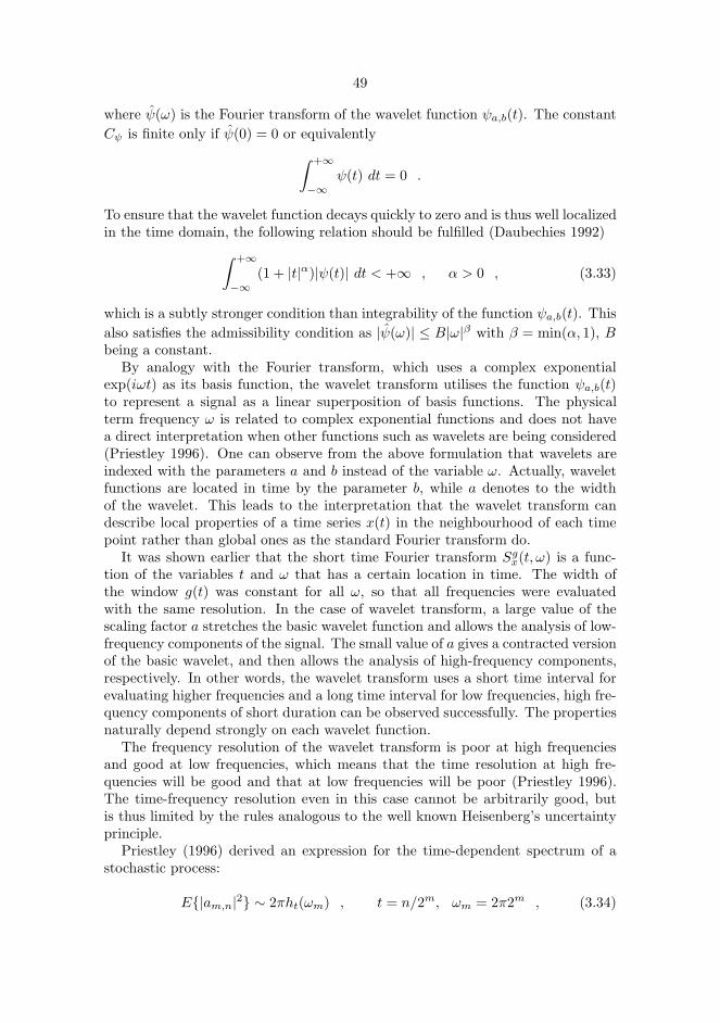
49

where ψ(ω) is the Fourier transform of the wavelet function ψa,b(t). The constantCψ is finite only if ψ(0) = 0 or equivalently∫ +∞

−∞ψ(t) dt = 0 .

To ensure that the wavelet function decays quickly to zero and is thus well localizedin the time domain, the following relation should be fulfilled (Daubechies 1992)∫ +∞

−∞(1 + |t|α)|ψ(t)| dt < +∞ , α > 0 , (3.33)

which is a subtly stronger condition than integrability of the function ψa,b(t). Thisalso satisfies the admissibility condition as |ψ(ω)| ≤ B|ω|β with β = min(α, 1), Bbeing a constant.

By analogy with the Fourier transform, which uses a complex exponentialexp(iωt) as its basis function, the wavelet transform utilises the function ψa,b(t)to represent a signal as a linear superposition of basis functions. The physicalterm frequency ω is related to complex exponential functions and does not havea direct interpretation when other functions such as wavelets are being considered(Priestley 1996). One can observe from the above formulation that wavelets areindexed with the parameters a and b instead of the variable ω. Actually, waveletfunctions are located in time by the parameter b, while a denotes to the widthof the wavelet. This leads to the interpretation that the wavelet transform candescribe local properties of a time series x(t) in the neighbourhood of each timepoint rather than global ones as the standard Fourier transform do.

It was shown earlier that the short time Fourier transform Sgx(t, ω) is a func-tion of the variables t and ω that has a certain location in time. The width ofthe window g(t) was constant for all ω, so that all frequencies were evaluatedwith the same resolution. In the case of wavelet transform, a large value of thescaling factor a stretches the basic wavelet function and allows the analysis of low-frequency components of the signal. The small value of a gives a contracted versionof the basic wavelet, and then allows the analysis of high-frequency components,respectively. In other words, the wavelet transform uses a short time interval forevaluating higher frequencies and a long time interval for low frequencies, high fre-quency components of short duration can be observed successfully. The propertiesnaturally depend strongly on each wavelet function.

The frequency resolution of the wavelet transform is poor at high frequenciesand good at low frequencies, which means that the time resolution at high fre-quencies will be good and that at low frequencies will be poor (Priestley 1996).The time-frequency resolution even in this case cannot be arbitrarily good, butis thus limited by the rules analogous to the well known Heisenberg’s uncertaintyprinciple.

Priestley (1996) derived an expression for the time-dependent spectrum of astochastic process:

E{|am,n|2} ∼ 2πht(ωm) , t = n/2m, ωm = 2π2m , (3.34)

50

which allows the squared modulus of wavelet coefficients to be interpreted as atime-dependent spectrum. It is assumed here that the mother wavelet has a com-plex form ψ(t) = exp(2πit), and its squared Fourier transform |ψm(ω)|2 is suitablyconcentrated around ω = ωm. Although the term frequency should be understoodwith care and in a somewhat heuristic sense, time-frequency analysis is probablyone of the most powerful features of the wavelet approach in this context.

3.5.2. Discrete wavelet transform

By choosing fixed values a = am0 and b = nb0am0 , m,n = 0,±1,±2, . . ., we get for

the discrete wavelet transform (DWT) (Daubechies 1992):

Wx(m,n) = 〈x(t), ψm,n(t)〉

=∫ +∞

−∞x(t)ψm,n(t) dt = a

−m/20

∫ +∞

−∞x(t)ψ(a−m0 t− nb0) dt .

Values a0 = 2 and b0 = 1 construct discrete wavelets ψm,n(t) = 2−m/2ψ(2−mt−n)used in multiresolution analysis constituting an orthonormal basis for L2(R).

To obtain a complete characterization of x(t) using discretized wavelets ψm,n(t),and further, to recover x(t) from the discrete transform in a numerically stablemanner, wavelet function should constitute a frame. The transform between thesignal and the wavelet function should be bounded above and below:

A ||x(t)||2 ≤∑m,n

|〈x(t), ψm,n(t)〉|2 ≤ B ||x(t)||2 (3.35)

with A > 0, B <∞. If frame bounds A and B are equal, then the frame is calledtight.

3.5.3. Multiresolution wavelet analysis

In multiresolution analysis successive approximation subspaces Vj fulfill the prop-erty Vj ⊂ Vj+1 with

∪+∞j=−∞Vj = L2(R) and ∩+∞

j=−∞ Vj = 0 .

The multiresolution feature follows from the condition that all the spaces are scaledversions of the central space V0:

x(t) ∈ Vj ⇐⇒ x(2j ·) ∈ V0 .

The space V0 has to be also invariant under integer translation:

x(t) ∈ V0 ⇒ x(· − n) ∈ V0

51

for all n ∈ Z. A scaling function φm,n(t) ∈ V0 is also required which is an or-thonormal basis in V0, where φm,n(t) = 2−m/2φ(2−mt− n). Under these assump-tions, the multiresolution scheme involves an orthonormal wavelet basis of L2(R),ψm,n(t) = 2−m/2ψ(2−mt− n), so that

Pm−1x(t) = Pmx(t) ++∞∑

n=−∞〈x(t), ψm,n(t)〉ψm,n(t) ,

where Pm is the orthogonal projection onto space Vm. The signal x(t) is conse-quently obtained by

x(t) =+∞∑

m,n=−∞〈x(t), ψm,n(t)〉ψm,n(t) .

The decomposition of the signal x(t) using discrete analysis wavelet functionsψj,k(t) and discrete scaling functions φK,k(t) can be given on different scales asfollows:

x(t) =K∑j=1

∞∑k=−∞

dj(k)ψj,k(t) +∞∑

k=−∞aK(k)φK,k(t) ,

where dj(k) are the wavelet coefficients (detailed signals) at scale 2j and aK(k) isthe scaling coefficients (approximated signal) at scale 2K . In Figure 3.2, the ideaof discrete wavelet analysis is presented by means of a wavelet decomposition tree.A decomposition onto dyadic scales associates the frequency content of the signaland scales as

2−j π ≤ ∆ωj ≤ 21−j π

for j = 1, 2, . . . . The signal spectrum includes the range 0 − π rad and ∆ωj is thefrequency band corresbonding the level j.

3.5.4. Subband filtering

Multiresolution analysis comprises a hierarchical and fast scheme to compute thewavelet coefficients of an analyzed signal. The scheme involves the computation ofsequentially coarser approximations of x(t) and the difference in signals betweentwo consecutive levels. In the subband filtering approach the computation consistsof the analysis and the synthesis steps which correspond to the decomposition andthe reconstruction stages in wavelet analyses (Strang & Nguyen 1996). The dis-crete wavelet transform can be implemented by the scaling (lowpass) and wavelet(highpass) filters

h(n) =1√2〈φ(t), φ(2t − n)〉 (3.36)

andg(n) =

1√2〈ψ(t), φ(2t − n)〉 = (−1)nh(1− n) (3.37)

52

Fig. 3.2. A wavelet signal decomposition presented by a tree structure.

being quadrature mirror filters (QMF) (Daubechies 1992). The estimation of thedetail signal at level j will be done by convolving the approximate signal at levelj−1 with the coefficients g(n). Convolving the approximate signal at level j−1 withthe coefficients h(n) gives an estimate for the approximate signal at level j. Theanalysis step (decomposition stage) involves filtering the approximate signal andretaining every other sample of the filter output (downsampling). The synthesisstep then involves upsampling and filtering to obtain a reconstructed signal. InFigure 3.3, the decomposition and reconstruction stages in a subband filteringscheme establishing a filter bank are presented.

3.5.5. Wavelet packet analysis

If one defines the scaling function W0(t) = φ(t) and the wavelet function W1(t) =ψ(t), then we can write for functions Wm(t), m = 0, 1, 2, . . ., as

W2m(t) = 22N−1∑n=0

h(n)Wm(2t− n) (3.38)

and

W2m+1(t) = 22N−1∑n=0

g(n)Wm(2t− n) . (3.39)

53

x(t)-

- h(n)

Decomposition

- ?2 - - 62 - h′(n)

Reconstruction

-

-x(t)

- g(n) - ?2

Downsampling

- - 62

Upsampling

- g′(n) -

Fig. 3.3. A schematic presentation of a subband filtering procedure using filter

banks. The operations ↓ 2 and ↑ 2 stand for downsampling and upsampling

by two.

The analyzing functions called wavelet packet atoms are given in an orthogonalcase as

Wj,m,n(t) = 2−j/2Wm(2−jt− n) , (3.40)

where j is a scale parameter, n is a time-localization parameter and parameter mgives roughly the number of “cycles” included in the oscillating waveform. Waveletpacket can be considered as a waveform whose oscillations persists for many cyclesbut are still finite. With fixed value of j the function Wj,m,n(t) analyzes the signalaround the position 2j · n at the scale 2j . The analyzed frequencies are roughlygiven by n/2N with n = 0, 1, . . . , (2j − 1).

Wavelet packet analysis is a generalization of wavelet analysis offering a richerdecomposition procedure. Both detailed and approximated signals are split ateach level into finer components. A set of details and approximations is called thewavelet packet decomposition tree.

3.5.6. Optimization of the wavelet packet decomposition

Wavelet (multiresolution) decomposition allows searching an optimal decomposi-tion among L trees if a signal of length N = 2L has been decomposed at L levels.Wavelet packet analysis involves the selection of an optimal decomposition treeamong at most 2L different subtrees of depth L. The optimization can be basedon e.g. the minimization of the entropy of analyzed signal, where the optimizeddecomposition is called the best tree. The idea is to look at each node of the decom-position tree and quantify the information to be gained by performing each split.

54

Fig. 3.4. A wavelet packet signal decomposition presented by an optimized

tree structure.

The entropy can be obtained by many approaches, for example, the Shannon en-tropy (Coifman & Wickerhauser 1992) is defined as E(x) = −

∑t x

2(t) · log(x2(t)).In Figure 3.4, the optimized wavelet packet decomposition tree is shown, whichschematically presents the idea of this procedure.

3.5.7. “De-noising” the signal

A possible application of the discrete wavelet analysis is to remove undesired com-ponents (noise) from the signal through a de-noising approach (paper III). Ba-sically the procedure includes decomposing the signal into the detail componentsdescribed above, identifying the noise components and reconstructing the signalwithout those components. This is called the linear denoising approach. The lineardenoising approach assumes that the noise can be found within certain scales, forexample, at the finest scales when the coarsest scales are assumed to be noise free.More sophisticated de-noising can be done by applying the non-linear threshold-ing approach, which involves discarding the details exceeding a certain limit. Thisapproach assumes that every wavelet coefficient contain noise and it is distributedover all scales.

The non-linear de-noising by both soft- and hard-thresholding methods can be

55

performed (Donoho 1995). The soft thresholded wavelet coefficients will be

η(dj(k)) ={

sign(dj(k)) · (|dj(k)| − p), if |dj(k)| > p0, if |dj(k)| ≤ p , (3.41)

where p is the applied threshold. The wavelet coefficients whose absolute valuesare lower than the threshold, are first set to zero, and then the remaining nonzerocoefficients are shrunk towards zero. With hard thresholding, the thresholdedcoefficients will be

η(dj(k)) ={dj(k), if |dj(k)| > p0, if |dj(k)| ≤ p , (3.42)

which simply means setting to zero the absolute coefficients lower than the thresh-old p.

In paper III, the assumed model for a noisy signal was x(t) = f(t) + e(t), wheref(t) is the noise free signal and e(t) is the white or non-white noise of variance δ2.The performance of the methods was evaluated from the simulations with L2-normgiven by the equation

||fo − xi||2 = (∑t

|fo(t)− xi(t)|2)1/2 , (3.43)

where fo denotes the original ECG signal being the same for all simulations, andxi denotes the ECG signal with added noise after noise removal.

3.5.8. Selection of the threshold

In paper III, the threshold p was selected for each signal using four thresholdestimation procedures: sure, heuristic sure, fixthres and minimax principles.The aim was to compare the performance obtained by different methods in thenoise removal of ECG signal. Stein’s Unbiased Risk Estimate (sure) (Donoho1993, Donoho & Johnstone 1995) is an adaptive threshold selection rule definedas p =

√2 · loge(n · log2(n)), where n is the number of samples in the signal

vector. With this approach obtaining risks and minimizing them with respect top values gives a threshold selection. The method is adaptive through searching athreshold level for each wavelet decomposition level. A fixed threshold approachfixthres calculates the threshold with respect to the length of the signal andthe estimated threshold is given by p =

√2 · loge(n) (Donoho & Johnstone 1994).

The heuristic sure approach being a variant of the first, replaces in very noisyconditions the sure with fixthres estimate (Misiti et al. 1996). Further, theminimax procedure applies a fixed threshold p = 0.3936 + 0.1829 · log(n) (Misitiet al. 1996) to produce the so called minimax performance for mean square erroragainst an ideal case (Bruce & Gao 1996, Donoho & Johnstone 1994).

The underlying signal model in paper III assumes the noise being normally dis-tributed with zero mean and variance of 1, which means that we have to rescale the

56

threshold values when dealing with unscaled and nonwhite noise. When normallyand uniformly distributed noises were studied, calculated thresholds were rescaledby the standard deviation of noise estimated from the finest level of the decompo-sition of each signal so that p = p · δ. Further, with AR(4)-noise the noise levelwas estimated scale by scale to take account the obviously strong high-frequencycontent. In wavelet approach, this was done by calculating δ for all scales. Inwavelet packet case, δ was estimated from the first node at each subdecompositionband which gave the best statistics for the noise level estimation. As a robustestimate of the standard deviation δ = Median(|dj(k)|)/.6745 was used (Donoho& Johnstone 1994).

3.6. Chaotic modelling

There are numerous investigations into fractal properties (Yamamoto & Hughson1993, Yamamoto et al. 1995, Yeragani et al. 1993) and chaos (Babloyantz & Des-texhe 1988, Signorini et al. 1994, Yamamoto et al. 1993) in HRV. The parametersused to assess the latter have included spectral analysis, correlation dimensions,Kolmogorov entropy and Lyapunov exponents. The most recent discussions haveconcerned chaotic modelling as applied to RR interval time series (Cohen et al.1996, Karrakchou et al. 1996) and especially to non-stationary time series (Kar-rakchou et al. 1996).

Cohen et al. (1996) studied the logistic equation (Poincare equation)

x(t) = A x(t− 1)(1− x(t− 1)) , 2 ≤ A ≤ 4 (3.44)

and some of its solutions as an example of a chaotic system. Here the first orderPoincare plot (first order difference plot) was introduced by presenting x(t + 1)vs. x(t), and given as a measure of the degree of chaos in a system. In Huikuriet al. (1996) an ellipse was fitted to the plot, and the centroid of this ellipseand the lengths of both axes were determined. In some earlier studies the firstorder Poincare plot called a “scattergram”, was shown to be capable of detectinglarge, abrupt deviations in heart rate (Baevskij et al. 1984, Baselli & Cerutti 1985,Stinton et al. 1972). The second-order difference, obtained by presenting (x(t+ 2)- x(t+ 1)) vs. (x(t+ 1) - x(t)), would show the degree of theoretical chaos (Cohenet al. 1996). The first order and second order difference plots are shown in Figure3.5.

A quantitative measure of the degree of variability in the second-order differenceplot, the measure of central tendency (CTM), takes the form

CTM =∑N−2

t=1 δ(d(t))N − 2

, (3.45)

where

δ(d(t)) ={

1 , if√

(x(t + 2)− x(t+ 1))2 + (x(t + 1)− x(t))2 < r0 , otherwise

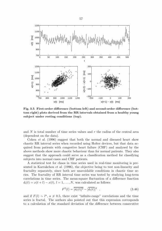
57

0 50 100 150 200 250 300 350 400 450 500700

800

900

1000

1100

1200

t

x(t)

[m

s]

700 800 900 1000 1100 1200700

800

900

1000

1100

1200

x(t) [ms]

x(t+

1)

[ms]

−200 −100 0 100 200−200

−100

0

100

200

x(t+1) − x(t) [ms]

x(t+

2) −

x(t

+1)

[m

s]

Fig. 3.5. First-order difference (bottom left) and second-order difference (bot-

tom right) plots derived from the RR intervals obtained from a healthy young

subject under resting conditions (top).

and N is total number of time series values and r the radius of the central area(dependent on the data).

Cohen et al. (1996) suggest that both the normal and diseased heart showchaotic RR interval series when recorded using Holter devices, but that data ac-quired from patients with congestive heart failure (CHF) and analysed by theabove methods show more chaotic behaviour than for normal patients. They alsosuggest that the approach could serve as a classification method for classifyingsubjects into normal cases and CHF patients.

A statistical test for chaos in time series used in real-time monitoring is pre-sented in Karrakchou et al. (1996), the objective being to test non-linearity andfractality separately, since both are unavoidable conditions in chaotic time se-ries. The fractality of RR interval time series was tested by studying long-termcorrelations in time series. The mean-square fluctuation of a difference functiondl(t) = x(t+ l)− x(t), l = 1, . . . , N , was calculated as follows

F 2(l) = [dl(t)]2 − [dl(t)]2 , (3.46)

and if F (l) ∼ la, a 6= 0.5, there exist “infinite-range” correlations and the timeseries is fractal. The authors also pointed out that this expression correspondsto a calculation of the standard deviation of the difference between consecutive

58

R peaks for different interval lengths. Non-linearities in RR intervals were testedusing Keenan’s test (Keenan 1985) with the hypothesis of linearity vs. second-order Volterra expansion. If any multiplicative term was found in the expansion,the time series was non-linear. A similar procedure for analysing correlations withthe mean fluctuation function was performed by Peng et al. (1993).

Several popular methods exist for studying chaos in cardiovascular time series,but the indices proposed for measuring it should be applied cautiously and resultsobtained should be interpreted with care. The basic condition is the need for largeamounts of data which make these methods not well-suitable for real-time analysis(Karrakchou et al. 1996). The problem also lies in discriminating a chaotic systemfrom a random one, calculation of the correlation dimension, for example, can giveincorrect results in a random time series (Osborne & Provenzale 1989). A randomsignal having a power spectrum like 1/fλ, λ > 0, for example, can erroneouslybe concluded as chaotic when estimating the correlation dimension (Theiler et al.1992). This point should be taken into account because HRV, in particular withlong data sets, has a power spectrum inversely related to frequency. A recentdevelopment has occured in developing statistical tests for chaos identification inHRV (Kanters et al. 1994, Karrakchou et al. 1996, Khadra et al. 1997). Kanterset al. (1994) showed the lack of low-dimensional chaos in RR interval time seriesacquired from healthy subjects and demonstrated the remarkably non-linear natureof RR interval time series. In Khadra et al. (1997), HRV signals obtained fromthe transplant patients were first detected random, but changed to chaotic astime passed after the operation. It was concluded by Kanters et al. (1994) andKarrakchou et al. (1996), alongside the adoption of a certain critical point of view,that chaotic modelling could be applied to the monitoring of RR interval timeseries whether these were chaotic or not.

4. Experimental settings

4.1. RR interval data

RR inteval recordings shown in paper I were made using an ambulatory heartrate recorder, which has recently been developed and stores timed occurences ofheart beats and sequences including numerous samples of ECG signals (Ruha et al.1997). The timing accuracy of the device is reported to be 1 ms, and it can storethe RR interval data over 24 hours. Examples on the RR interval analyses wereproduced using Matlab software (The Mathworks, Inc., Natick, MA, USA).

4.2. Dynamics of the ventricular repolarization duration

4.2.1. Measurement equipment and software

The ECG was acquired in paper II by Medilog EXCEL-2 ver. 7.5 Holter Man-agement System (Oxford Medical, Ltd., UK) using a two-channel tape recorder(model MR-45), which contains a C60 cassette as a recording medium. The datawere replayed from the recorder by the Holter software and stored on the harddisk of a PC computer with 128 Hz sampling rate and 8 bits resolution. The rawECG data on the channel 2 (lead II) was read from a file by a program designedspecifically for the beat-to-beat measurement of RR and QT intervals.

The program was designed to operate within the Windows environment on astandard PC. The program code was written using Borlands Turbo C++ -compiler(Borland 1991) (Borland International, Inc., USA). The aim was to develop amodular program structure, which is easy to maintain and can be flexibly expandedwith new features. Therefore, the program was divided into separate modules.Options for loading the digitized ECG data and displaying data with detectionof waveforms are included. The preprocessing and waveform detection proceduresperform the analysis based on the theory described in the particular paragraphs inthis thesis. The ECG signal can be optionally interpolated in order to increase the

60

precision of the waveform measurement. The resulting time series (RR and QTintervals) can be shown on a beat-to-beat basis as a function of the beat number.In a scatterdiagram each QT interval value is drawn as a function of the previousRR interval value, i.e. QT (t) vs. RR(t− 1), and a regression line is fitted to thedata by minimizing the least square error. The program also offers options forexporting the resulting time series and the analyzed ECG as well as for modifyingseveral program parameters.

4.2.2. Testing of the automatic waveform measurement

4.2.2.1. Real ECG signals

Ambulatory ECG was acquired from six healthy subjects to test the automaticwaveform analysis procedure. A ten minute section of ECG was selected fromeach recording and analyzed by using the different options of the program. ECGshad upward R peaks and clear T wave shapes.

The effect of the interpolation of the ECG on the interval variability measure-ment as well as the effect of different QT interval onset and T wave end positiondefinitions were tested. The “QT interval” onset definitions were true QRS onset(Q), R wave maximum (R), ascending (Ra) or descending (Rd) maximal slopesof R wave. The “T wave end” position definitions were the peak (maximum,Tmax) and end of T wave (Te). Combinating these definitions produced a set of“QT interval” time series: QTe, QTmax, RaTe, RaTmax, RTe, RTmax, RdTe andRdTmax.

4.2.2.2. Simulated ECG signals

Simulated ECGs were generated by obtaining a cardiac cycle from each abovementioned ECG strips and repeating the cycle 600 times. Simulated noise freeECGs were then corrupted with six types of noises at different noise levels, seeTable 4.1. Simulations 1-5 were additive noise and summed with the ECG. A sinewave with a frequency varying at 0 - 0.5 Hz (simulation 1) was constructed as

x(t) = sin(2 · π · 0.25 · t− 7.645 · π · sin(2 · π · t/96)) (4.1)

and a sine wave with a frequency varying at 3 - 5 Hz (simulation 2) was generatedas

x(t) = sin(2 · π · 5 · t− 12.944 · π · sin(2 · π · t/20)) (4.2)

with t = 1, . . . , N .Amplitude modulation (AM) in simulation 6 was constructed as follows (Ziemer

& Tranter 1990)x(t) = [1 + a ·mn(t)] · y(t) , (4.3)

61

where x(t) is the modulated signal and y(t) is the ECG signal. mn(t) is a uniformlydistributed noise normalized such as the minimum value of mn(t) is -1. Theparameter a is called as the modulation index (0 ≤ a ≤ 1).

The objective was to measure the sensitivity of the automatic measurement ofthe repolarization duration using commonly-occurring noise types. This type ofanalysis is especially necessary, because the variability of the repolarization dura-tion is very low, thus, the various disturbances on ECG can produce inaccuraciesin this time period measurement. Typically, QT interval variability is sd = 4-5ms as RR interval variability can be sd = 60-70 ms. The noise level was definedwith the signal-to-noise ratio (SNR) in decibels (dB) as

SNR = 20 log(σcycle

σnoise) , (4.4)

where σcycle is the root-mean-square (rms) value of the ECG signal obtained fromthe whole cardiac cycle and σnoise is the rms value of the additive noise signal,respectively. For instance, 10 % relative rms value of the noise signal gives 20 dBSNR value. The effects of different noise types were measured at noise levels of 5- 50 dB.

Table 4.1. Simulated noise types used in the noise sensitivity measurement.

Simulation Noise type Simulated effect

1 0 - 0.5 Hz sine wave Baseline wander due to breathing2 3 - 5 Hz sine wave Motion artefacts3 50 Hz sine wave Mains noise4 Gaussian white noise EMG, motion artefacts5 Sum of the noise Mixed effect

realizations 1 - 46 Uniformly distributed Amplitude modulation

amplitude modulation due to breathing

62

4.3. Denoising of an ECG signal

In paper III, fifty independent simulations were used to evaluate the performanceof the applied denoising methods. Simulations were created by adding three typesof the noise on a noise free ECG: gaussian and uniformly distributed white noise,and non-white noise generated by an autoregressive (AR) model of order 4. Thenoise amplitudes were scaled so that the signal-to-noise ratio was 5 dB for allsignals. The performances of the methods were studied by obtaining errors withinan ECG including 2600 samples and more specifically obtaining errors within sixQRS-complexes extracted manually from the whole ECG. The latter approachallowed the investigation of the performance of the denoising methods to handlethe high frequency parts of the ECG. Matlab software was utilized with WaveletToolbox to perform wavelet analysis for the digitized ECG signal obtained froman anesthesized monkey. A 512 Hz sampling frequency was used with a resolutionof 12 bits.

When considering the compactly supported orthogonal wavelet families (Dau-bechies, Symlets, Coiflets) with discrete transform, the Coiflet wavelet basis wasfound most suitable. The denoising performances were very near between thesefamilies, however, Coiflets showing slightly the best performance. The Coifletwavelet (Coif5) of order N = 5 was used which had lowest denoising error amongCoiflet functions. The error performance was measured with L2-norm given byEquation 3.43. The Coif5 function is a near symmetrical wavelet, which is com-pactly supported with maximum number of vanishing moments for a given supportwidth (6N − 1), Figure 4.1a. The analysis done by Coif5 wavelet is orthogonal.Wavelet packet analysis was made by Coiflet wavelet packet function Wj,m,n(t)with m = 5, see Figure 4.1b. The wavelet packet decomposition was optimized byminimizing the Shannon entropy (section 3.5.6).

4.4. Analysis of APD time series

4.4.1. Patients

In paper IV, 12 ordinary cardiology patients (six males and six females), under-going routine electrophysiological testing for symptomatic cardiac arrhythmias,were included in the study. However, the intended study was not the reasonthese patients were tested. None of the patients had clinical or echocardiographicevidence of structural heart disease. The clinical indication for the studies wassymptomatic supraventricular tachycardia in all patients. All cardiac medicationshad been stopped at least four days before the studies.

63

6 8 10 12 14 16 18 20 22−1

−0.5

0

0.5

1

1.5

(a)

1200 1400 1600 1800 2000 2200 2400 2600 2800−1.5

−1

−0.5

0

0.5

1

1.5

2

(b)

Fig. 4.1. (a) A Coiflet wavelet used for a discrete wavelet analysis. (b) A

Coiflet wavelet packet used for a discrete wavelet packet analysis.

4.4.2. Study protocol

The recordings of MAP signals in sinus rhythm and during constant rate pacingwere performed after the diagnostic electrophysiological study. Quadripolar elec-trode catheter was introduced into the high right atrium and a bipolar Ag/AgClelectrode catheter was introduced (USCI, Division of C.R. Bard, Billerica, MA,USA) into the right ventricle. MAPs were obtained by gently pressing the tip ofthe catheter against the endocardial surface of the right ventricular apex. Thesignals were recorded on a CardioLab (Prucka Engineering, Inc., Houston, TX,USA) using 1024 Hz sampling rate with a resolution of 0.1 mV of the amplitudeof the signal. The MAP signals were amplified and filtered at frequencies of 0.05 -500 Hz. The amplitude (>10 mV) and stability of the signals were assessed beforerecordings.

The MAP signals were recorded in sinus rhythm during quiet normal respiration

64

for ten minutes. After baseline recordings in sinus rhythm, the high right atriumwas paced at the cycle length of 600 ms for ten minutes. Only those patientswith 1:1 atrioventricular (AV) conduction without significant fluctuation in theatriohisian conduction time with the atrial pacing at the cycle length of 500 mswere included.

4.4.3. Analysis of MAP signals

The CardioLab software was used to acquire the MAP data from patients. TheMAP Analysis program was written in Pascal 7.0 language (Borland International,Scotts Valley, CA, USA) to be used with CardioLab equipment on a standardPC under a DOS or a Windows environment. The program processes MAPsand calculates the amplitude, RR interval, and the 15 %, 30 %, 50 % and 90% repolarization times producing a series of results calculated from successivewaveforms, see Figure 1 in paper IV. There is a possibility to edit manually theautomatic analysis. Changing the baseline updates all the calculated results. Itis also possible to discard a waveform distorted by noise and exclude it from thefinal results.

4.4.4. Analyses of variability of RR intervals and actionpotential duration

Two-dimensional vector analyses of variability of RR interval and action potentialduration (APD) time series were performed by a method described previously(Huikuri et al. 1996). Poincare plots were generated where each time series valueis plotted as a function of the previous value for a predetermined length of timeseries. Quantitative analysis of the plots involves fitting an ellipse to the plotand estimating the long and short term time series variability from the lengthsof the axes of the ellipse. The Poincare plots of RR intervals and APD at the90 % (APD90) and 50 % (APD50) of repolarization were generated for the twosegments of five minute periods in sinus rhythm and one segment of five minuteperiod at the end of the pacing (i.e., five minutes after the onset of constant ratepacing) at which point the APD had reached its steady-state level. The segmentswith ectopic beats, artifacts, and distortion of the MAP signals were edited bothmanually and automatically and deleted before analyses.

Paired t-test was used to compare the measures of variability of APD and RRintervals in sinus rhythm during pacing. Pearson correlation coefficient was usedto assess the univariate correlations between the measures of variability. p < 0.05was concidered significant.

65

4.5. Wavelet analysis of HRV

RR inteval recordings analyzed in section 5.4 were made using Medilog EXCEL-2ver. 7.5 Holter Management System (Oxford Medical, Ltd., UK). RR interval datawas further processed using HEARTS software (Heart Signal Oy, Oulu, Finland)to exclude inappropriate intervals. Time series were then resampled using 2.4Hz sampling frequency to obtain an equidistantly sampled data. Analyses wereperformed using Matlab software with Wavelet Toolbox (The Mathworks, Inc.,Natick, MA, USA) at the Center for Scientific Computing, CSC (Espoo, Finland).

The Coiflet wavelet and wavelet packet functions of order 5 were used to obtainthe corresponding spectra (Figure 4.1). The optimization of the wavelet packetdecomposition was performed by minimizing the Shannon entropy (section 3.5.6).

RR interval recordings after noradrenaline injections were analyzed from eighthealthy subjects. Recordings included a baseline period before drug administra-tion, which was continuously increased using 50, 100 and 150 ng injections. Asecond set of RR interval data was collected from ordinary cardiology patientsduring several hours prior to ventricular fibrillation. The wavelet analysis wasdone within one hour before the event for 11 patients.

5. Results

5.1. Dynamics of the ventricular repolarization duration

5.1.1. Interpolation of the ECG

A standard Holter recording frequency of 128 Hz is not sufficiently robust to cap-ture the low level of QT interval variability found in most patients. Therefore, ahigher sampling rate is needed to obtain precise measurements. An important aimof this study was to test the feasibility of interpolation as a means of increasingthe fidelity of an ECG initially digitized at the low Holter sampling rate. However,the disadvantage of the interpolation is that the features of the ECG cannot bebetter resolved than the original digitized ECG allows. Interpolation of the ECGallows a better time resolution for time interval variability measurement.

In the present study the ECG recordings were interpolated to 256, 512, 768 and1024 Hz to illustrate the changes in the resolution of QT interval variability. Forexample, in a RTmax time series obtained from an original ECG signal sampledat 128 Hz, the natural variability can not be seen (Figure 2, top, in paper II). Incontrast, the same recording interpolated to 1024 Hz shows the existing variabilitymore clearly (Figure 2, bottom, in paper II). This method also provides a meansto obtain a proper time series distribution for analysis.

5.1.2. RMSSD of QT interval time series

The rmssd value is a simple and traditional measurement of the variation in acardiovascular variability signal. The absolute rmssd values (ms) of a QT timeseries with different T wave end definitions (Tmax and Te) as a function of samplingfrequency for one patient are presented in Figure 5.1. The variability decreases inall QT time series as ECG is interpolated, reaching a maximal efficiency at about1 kHz. At 1024 Hz, the rmssd values are 25-30 % and 40-60 % lower comparedto 128 Hz for Te and Tmax, respectively.

67

0 500 10002

3

4

5R

MS

SD

[m

s]

f [Hz]

0 500 10002

3

4

5

RM

SS

D

[ms]

f [Hz]

(a) (b)

Fig. 5.1. The absolute rmssd values of QT interval time series using (a) Tmax

and (b) Te definition. Abbreviations for the QT interval onset definition:

true QRS onset, Q (4); ascending maximal slope of R wave, Ra (◦); R wave

maximum, R (+); and descending maximal slope of R wave, Rd (×).

Furthermore, at 1024 Hz sampling frequency the variability observed in timeseries with Tmax definition is about 40 % lower than the variability with Te def-inition. Remarkable differences in variabilities do not typically exist due to thedefinition of the start of the repolarization duration. Defining the start of repo-larization duration at the maximum or at the descending maximal slope of theR wave, gives slightly smaller variability than the other choices. Looking for theonset of Q wave produces the largest variability in time series. The 40% differencebetween Tmax and Te observed in the rmssd interpolated at 1024 Hz, may be dueto the increase in noise at Te resulting in an increase in the signal variability atthat end-point. The start-point for the measurement of QT can be defined as Q,Ra, R or Rd. For the Tmax end-point, differences among these starting points wereobserved with Q displaying the greatest variability and Rd the least.

The rmssd values of RTmax and RTe time series for the six patients measuredis shown in Figure 5.2. This example demonstrates the reproducibility of thevariability measurement when interpolating the ECG signal. Defining the onsetof the QT interval at the maximum of the R wave and the offset of the T wave atthe maximum of T wave, seems to give a reproducible variability measurement.

68

0 500 10002

3

4

5

6

7

RM

SS

D

[ms]

f [Hz]

0 500 10002

3

4

5

6

7

RM

SS

D

[ms]

f [Hz]

(a) (b)

Fig. 5.2. rmssd values of (a) RTmax and (b) RTe interval time series obtained

from six patients.

5.1.3. Power spectrum estimates

In order to evaluate further the applicability of our algorithm, we also used powerspectrum estimates to quantify the QT interval variability. RR, RTmax and RTe

interval time series from one patient was obtained by an ECG interpolated to1024 Hz (Figure 5.3). The power spectrum estimates are presented in Figure5.4. All power spectra show a clear peak at f = 0.32 Hz which is probably due tobreathing. In addition to the sum spectrum the spectra of the separate componentsare estimated.

The power estimates of the main component observed at f = 0.32 Hz in theRTmax and RTe spectra were plotted as a function of the sampling rate (Figure8 in paper II). As was demonstrated with rmssd, the power estimates decreaseas the sampling rate increases. At sampling frequency of 1024 Hz, the estimatedpower of the main peak for the power spectrum of the RTmax time series was 56 %of that estimated for RTe time series in terms of ms2. In this case, the total powersin the time series were 5.7 ms2 and 9.4 ms2 for RTmax and RTe, respectively.

69

0 50 100 150 200 250 300 350 400 450

1000

1200

1400

1600

RR

[m

s]

0 50 100 150 200 250 300 350 400 450

295

300

305

310

315

RT m

ax

[ms]

0 50 100 150 200 250 300 350 400 450

360

370

380

RT e

[ms]

t

Fig. 5.3. RR (top), RTmax (middle) and RTe (bottom) interval time series

obtained from patient 6.

70

0 0.05 0.1 0.15 0.2 0.25 0.3 0.35 0.4 0.45 0.50

1

2

3

4

5

6

7

8

9

10x 10

4

PS

D

[ms2 /

Hz]

f [Hz]

0 0.05 0.1 0.15 0.2 0.25 0.3 0.35 0.4 0.45 0.50

10

20

30

40

50

60

PS

D

[ms2 /

Hz]

f [Hz]

0 0.05 0.1 0.15 0.2 0.25 0.3 0.35 0.4 0.45 0.50

10

20

30

40

50

60

PS

D

[ms2 /

Hz]

f [Hz]

Fig. 5.4. Power spectrum estimates of RR (top), RTmax (middle) and RTe

(bottom) interval time series obtained from patient 6. The estimates repre-

sent the sum spectrum (solid line) and the spectra of the separate components

(dashed lines).

71

5.1.4. Simulated ECG signals

A critical step in the development of any QT algorithm is to determine the beststart and end points for ventricular repolarization to obtain an accurate estimate ofQT interval. To achieve this goal we compared the variability in the QT time seriesusing different start and end points. Simulations of six commonly-encounteredtypes of noise (Table 4.1) were used to ascertain which of eight possible intervalsproduced the least degree of variability for each noise type. These results arepresented in Tables 2 - 7 in paper II. The lower the sd value, the greater theprecision of the measurement. Overall, the intervals using RTmax and RdTmax

provided the most reliable results in most situations.The first type of noise was at 0-0.5 Hz, simulating baseline drift due to breathing

(Table 2, paper II). At low SNRs using Te as the endpoint of the QT interval givesthe most precise results. At levels of 25 dB and higher, it is better to use Tmax.For the simulation of motion artefacts (3-5 Hz), electrical line noise (50 Hz) andGaussian white noise (Tables 3 - 5, paper II), Tmax was consistently more precise.Summing the noise simulations 1-4 and adding them to the ECG signal producedsimilar results, i.e. Tmax is the most precise endpoint (Table 6, paper II). UsingQ as a start point showed greater variability and was therefore less precise thanusing R in most cases.

Noise due to breathing also contains an amplitude component and can be sim-ulated by amplitude modulation (Table 7, paper II). The mean sd values of allanalyzed time series are given as a function of the modulation index a, see section4.2.2.2. At values a ≤ 0.3, defining the end of the QT interval as Te, producedthe lowest variability. The results also indicate that choosing the onset of the QTinterval at the descending slope of R wave is the most insensitive to this kind ofthe simulated noise. It is interesting to note that measuring RR interval in casesof amplitude modulation produces lower variability than QT. In fact, measuringRR interval for each type of noise (Tables 7 and 8, paper II) overall showed lessvariability compared to measurements of QT interval.

The variability of RTmax as a measurement of QT interval among six differentpatients is shown in Table 9 in paper II. In each case the sum of each typeof simulated noise was added to the signal. Coefficients of variation (cv) werecalculated to study the amount of variability with respect to the mean value ofthe analyzed time series. According to the obtained cv values, the variability ofall QT time series were less than 11 % of the mean of each time series at all noiselevels. For example, at SNR of 30 dB, the percentage amounts of variability werebetween 0.24 - 0.47 % compared to the mean cv of 0.32 %.

The simulated noises were also added to the real ECG data in order to studythe effect on the real variability. As an example, sd values of RTmax time series ofpatient number 6 with different simulated noises are shown in Table 5.1. The SNRrefer here to the same noise amplitude as used with simulated ECGs above. sd

value of the original time series was 2.35 ms2. The signal variability with all noisetypes reached this level at SNR of at least 20-25 dB. With amplitude modulation(simulation 6), sd values were 9.63, 6.55, 3.12, 2.63 and 2.45 ms2 as a function ofdecreasing modulation index.

72

Table 5.1. sd values of the RTmax time series measured from patient n:o 6 withdifferent simulated noises.

SNR 0 - 0.5 Hz 3 - 5 Hz 50 Hz Gaussian Sum of the noisesine wave sine wave sine wave white noise realizations 1-4

dB ms ms ms ms ms

5 2.59 80.01 4.03 83.12 72.7710 2.46 38.45 3.24 29.45 17.6815 2.39 9.27 2.64 4.19 3.8020 2.37 3.41 2.48 3.04 2.8825 2.37 2.75 2.40 2.58 2.5530 2.37 2.54 2.42 2.42 2.4140 2.36 2.39 2.36 2.38 2.3850 2.35 2.36 2.36 2.36 2.37

5.1.5. Discussion

The analysis of the dynamics of RR or QT time series can only be performed byobserving the beat-to-beat variability in a time series. There is no “absolute” un-biased measurement of ventricular repolarization duration because even a manualmeasurement done by an experienced cardiologist is limited by the precision of thetool used. There also exists a natural variability between manual measurementsdone by different persons. All automatic measurement systems and algorithmsproduce some error in interval measurement as well. An automatic algorithm,however, rapidly analyses an ECG and the results can be reproducible. The per-formance and reproducibility can be compared between different measurementalgorithms and against manual measurement.

In previous studies, the ventricular duration variability has been reported to bevery low compared to RR interval variability. For instance, a study by Nollo et al.(1992) showed sd values of 2-6 ms depending on the definition of the measured timeinterval. Ambulatory ECGs are commonly acquired at a low sampling rate due tolack of the data storage capacity of the equipment. As it was shown in this study,an ECG sampled at 128 Hz can not be used to obtain the beat-to-beat variabilityin QT time series. Variability decreased as the sampling frequency of the ECGincreased, which is produced by the improved time resolution in the waveformanalysis. Due to these factors, an interpolation procedure was included in theanalysis scheme to obtain improved precision. The interpolation can significantlyimprove the resolution of the ventricular repolarization duration measurement,and the procedure can cause a minor distortion only in the QRS complex, but notin the T wave (Speranza et al. 1993).

The noise sensitivity of the implemented algorithm was tested with several types

73

of simulated noise. In this context, the testing was important, because QT intervalvariability is low, and therefore a significant part of the observed variability canbe due to noise. Until now, there have been only a few publications dealing withnoise sensitivity of QRS detection (Barbaro et al. (1991), Friesen et al. (1990),Koeleman et al. (1984) and Ruha et al. (1997)). Furthermore, there are only afew references, where the noise sensitivity of QT interval measurement is actuallyconsidered (Nollo et al. (1990), Nollo et al. (1992), Porta et al. (1996) and Speranzaet al. (1993)). The algorithm used in this work has not previously been systemicallytested with simulated noise.

Our noise simulations present the most common disturbances observed in am-bulatory electrocardiogram with precision reported as sd values. Six simulatedtest signals were constructed by adding noise to an “ideal” ECG. In addition, theeffect of the amplitude modulation of respiration were modelled as the uniformlydistributed amplitude modulation of the ECG. It should be noted that there mayexist different definitions of signal-to-noise ratio and the noise distribution shouldbe known.

Our simulations showed that, in most of the cases, defining the end of QTinterval at the maximum of the T wave gave most precise measurement of theventricular repolarization duration. However, when the shape of the T wave wasaltered by amplitude modulation (simulation 6) choosing the end of T wave pro-duced the lowest variability in a time series. This observation has also been madeby Porta et al. (1996). Adding a 0-0.5 Hz sine wave, using Tmax definition pro-duced larger variability in time series at lowest signal-to-noise ratios (SNR ≤ 20dB). These findings may suggest that the apex of the T wave is especially sensitiveto the noise due to breathing.

The definition of the onset of the ventricular repolarization duration is mostprecisely made on the maximum or descending maximal slope of the R wave.The choice between R and Rd definition in this waveform analysis algorithm maydepend on the quality of the measured signal. For example, if a particular Rwave has two peaks with variable amplitudes located very near to each other, thealgorithm may produce noise in a time series due to jitter when looking for themaximum of the R wave. The Q wave was often missing in the patient ECGs,which produced a lot of the noise in the QTe and QTmax time series.

In a previous study (Speranza et al. 1993) an ECG was sampled at 250 Hzand interpolated to 1024 Hz sampling rate. The algorithm was tested only withGaussian noise added at different noise levels. The coefficient of variation (cv) wasabout 1 % for RTmax and less than 4 % for the RTe time series at SNR = 40 dB.As a comparison, the mean cv values in our work, were 0.16 % and 0.20 %, withmean sd values of 0.42 ms and 0.70 ms, respectively (Table 5, paper II). Theseresults clearly show a better precision in the QT estimate. The SNR definition isassumed to be the same in both studies.

The analysis of dynamics of RR or QT time series can only be quantified byobserving beat-to-beat variability in time series. Furthermore, the periodic vari-ability in RR and QT time series can be observed by using power spectrum esti-mation. The results show that the estimated powers in QT time series are verylow compared to powers estimated in RR interval spectrum, as demonstrated in

74

earlier studies (Nollo et al. 1992, Speranza et al. 1993). However, power spectrumestimation by AR modelling seems to be capable of showing clear components alsoin time series with low variability.

In this study, differences were found in the noise sensitivity of the computeranalysis of ventricular repolarization when various definitions of QT interval wereused. In most cases, RTmax or RdTmax time series can be regarded as the mostprecise QT interval estimate. The results suggest that low amplitude variabilitymay be hidden by noise due to inadequate time resolution of the signal, breathing,muscle activity and motion artefacts. These factors may require a more criticalassessment of data obtained by either manual or automated analysis of QT intervaldynamics.

75

5.2. Wavelet transform based noise removal of ECG

Denoising performances of the four threshold selection methods are reported inTables 5.2 and 5.3 with optimal decomposition depths. Generally, denoising errorfirst decreased as the decomposition depth increased. The results were optimized inrespect of the minimum value of the error averages giving an optimal downsamplingdepth, which varied between denoising approaches. Methods are compared inwavelet and wavelet packet analyses applying both soft and hard thresholding.First the performance within the whole ECG strip including six cardiac cycleswas measured. The results show that wavelet denoising approaches had betteroverall denoising performances than wavelet packet approaches in all cases exceptwith the heuristic sure rule when using hard thresholding for white noises. Thewavelet methods were preferable in removing especially the AR(4)-noise, when theerrors were generally 2-5 times greater with wavelet packets (Tables 5.2 and 5.3).With other noise types the difference varied from a few to a few tens of percentsfor wavelet methods.

Table 5.2. Denoising performance of wavelet denoising approach. Values are meansand standard deviations of ||fo − xi||2. N(0,δ2) is normally distributed and zeromean noise with variance δ2, U[a,b] stands for a uniformly distributed noise andAR(4) is the non-white noise generated by an autoregressive model of order 4. doptis the optimal decomposition depth minimizing the denoising error.

Noise Thresholding Thresholding selection ruletype nonlinearity

sure heuristic fixthres minimax

sure

dopt dopt dopt dopt

N(0,δ2) soft 449.3±16.2 445.7±12.7 573.0±11.6 538.1±16.25 5 2 4

hard 660.8±74.0 539.9±19.8 444.5±12.0 531.9±24.84 4 4 4

U[a,b] soft 445.3±13.6 444.6±13.4 576.2±10.7 532.5±17.75 5 2 4

hard 646.4±64.6 543.5±19.4 446.3±17.0 526.0±25.64 4 4 4

AR(4) soft 363.5±20.7 363.3±14.1 394.2±13.3 390.2±13.54 4 2 2

hard 526.4±93.0 382.6±15.7 365.4±15.8 481.9±25.24 4 4 4

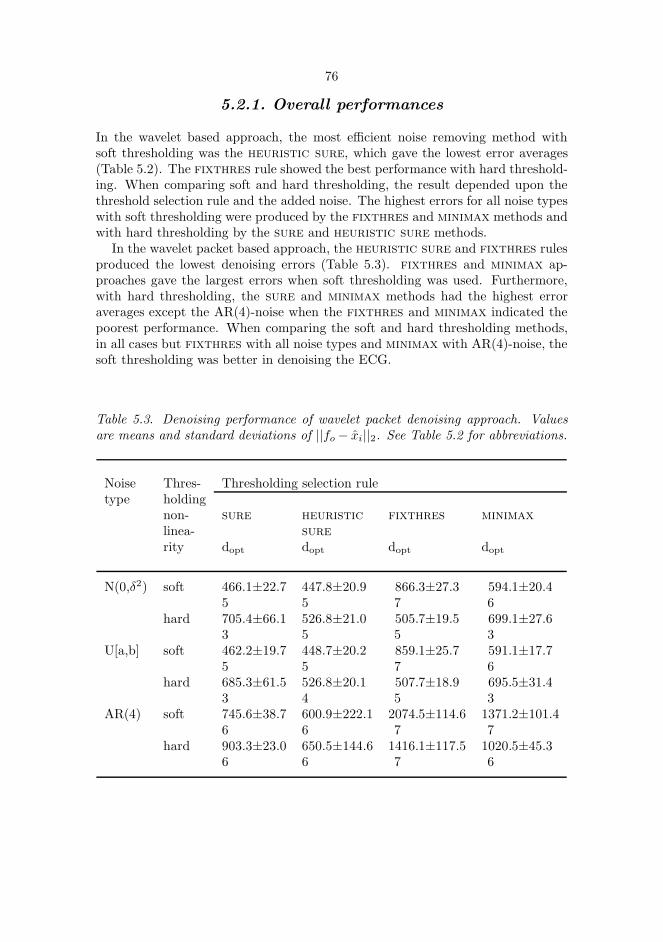
76

5.2.1. Overall performances

In the wavelet based approach, the most efficient noise removing method withsoft thresholding was the heuristic sure, which gave the lowest error averages(Table 5.2). The fixthres rule showed the best performance with hard threshold-ing. When comparing soft and hard thresholding, the result depended upon thethreshold selection rule and the added noise. The highest errors for all noise typeswith soft thresholding were produced by the fixthres and minimax methods andwith hard thresholding by the sure and heuristic sure methods.

In the wavelet packet based approach, the heuristic sure and fixthres rulesproduced the lowest denoising errors (Table 5.3). fixthres and minimax ap-proaches gave the largest errors when soft thresholding was used. Furthermore,with hard thresholding, the sure and minimax methods had the highest erroraverages except the AR(4)-noise when the fixthres and minimax indicated thepoorest performance. When comparing the soft and hard thresholding methods,in all cases but fixthres with all noise types and minimax with AR(4)-noise, thesoft thresholding was better in denoising the ECG.

Table 5.3. Denoising performance of wavelet packet denoising approach. Valuesare means and standard deviations of ||fo− xi||2. See Table 5.2 for abbreviations.

Noise Thres- Thresholding selection ruletype holding

non- sure heuristic fixthres minimax

linea- sure

rity dopt dopt dopt dopt

N(0,δ2) soft 466.1±22.7 447.8±20.9 866.3±27.3 594.1±20.45 5 7 6

hard 705.4±66.1 526.8±21.0 505.7±19.5 699.1±27.63 5 5 3

U[a,b] soft 462.2±19.7 448.7±20.2 859.1±25.7 591.1±17.75 5 7 6

hard 685.3±61.5 526.8±20.1 507.7±18.9 695.5±31.43 4 5 3

AR(4) soft 745.6±38.7 600.9±222.1 2074.5±114.6 1371.2±101.46 6 7 7

hard 903.3±23.0 650.5±144.6 1416.1±117.5 1020.5±45.36 6 7 6

77

5.2.2. Performances within QRS-complex

The ability of denoising methods to remove noise from the high frequency partsof ECG was studied by determing the error values within QRS-complexes, seeTables 5.4 and 5.5. The wavelet methods were more efficient to remove the AR(4)-noise, when the errors were upto 4 times greater with wavelet packets. However,wavelet packet approaches showed better performances than wavelet approachesin removing normally or uniformly distributed noise within QRS-area especially ashard thresholding was used. The sure method produced the lowest proportionalerror for the wavelet denoising using hard thresholding method for all noise types.With soft thresholding, except the AR(4)-noise, the fixthres had the lowestproportional error within QRS-area. In the wavelet packet approach, the lowestproportional error was indicated most often by sure or heuristic sure rules.Generally, denoising errors seem to concentrate on the QRS-area when the purewavelet approach is employed. The QRS-complex area included proportionally lesserror when hard thresholding was used, except the fixthres rule as the waveletdecomposition was used.

Table 5.4. Denoising performance of wavelet denoising approach measured withinQRS-complexes. Values presented are means and standard deviations of ||fo −xi||2. The decomposition depths are the same as in Table 5.2. See Table 5.2 forabbreviations.

Noise Thresholding Thresholding selection ruletype nonlinearity

sure heuristic fixthres minimax

sure

N(0,δ2) soft 286.2±21.4 300.5±18.5 258.5±10.6 445.8±18.4hard 274.6±25.4 259.9±12.2 319.7±16.7 287.9±17.9

U[a,b] soft 283.6±19.6 297.3±19.0 259.1±11.9 439.5±19.2hard 269.5±20.0 262.1±12.3 321.7±18.1 289.1±17.5

AR(4) soft 208.6±13.9 230.0±9.9 214.3±7.7 200.7±8.4hard 221.9±28.2 209.7±10.0 224.4±10.1 226.2±22.6

When comparing the performance within QRS-complexes using absolute er-ror measurement, heuristic sure or fixthres gave most often the lowest errorvalues for the wavelet approach. In the wavelet packet approach, the best perfor-mances were found by sure and heuristic sure rules. Further, hard thresholdingmethod gave lower absolute errors with all variations of denoising methods, whenthe wavelet packet approach was used. With pure wavelet denoising, results werethe same except with fixthres, when soft thresholding gave lower error. sure

78

Table 5.5. Denoising performance of wavelet packet denoising approach measuredwithin QRS-complexes. Values presented are means and standard deviations of||fo− xi||2. The decomposition depths are the same as in Table 5.3. See Table 5.2for abbreviations.

Noise Thresholding Thresholding selection ruletype nonlinearity

sure heuristic fixthres minimax

sure

N(0,δ2) soft 271.2±19.1 301.8±28.7 607.1±22.4 381.3±19.4hard 270.9±27.6 253.9±17.0 272.4±16.6 287.6±23.4

U[a,b] soft 267.1±18.0 300.5±27.7 602.7±23.2 377.5±18.6hard 264.9±24.8 264.4±16.4 276.5±16.1 286.6±18.2

AR(4) soft 324.0±34.1 308.8±39.9 866.2±61.6 562.5±32.2hard 320.8±23.2 258.3±42.7 493.8±36.9 391.4±33.7

and minimax showed also better denoising performance for the AR(4)-noise withsoft thresholding.

5.2.3. Checking the error signals

Because numerical error measures do not necessarily tell everything about noiseremoval, it is useful to check the denoised signals visually. There probably existsuch strange signal patterns which can not be predicted from error values. Itis important to see the error signal between the noisy and the denoised signal,because then one can observe how the error is localized within the cardiac cycle.In Figure 5.5, the successful result of denoising ECG with normally distributednoise by wavelet approach using the minimax method is shown. The error betweenthe original and denoised ECG is mainly concentrated within the QRS-complexes.

Sometimes performing the signal denoising does not mean that only the addednoise has been removed. ECG can be very clean after denoising and the errorsignal has a large amplitude, which means that the denoising method has notonly been robust in removing added noise but also has seriously altered the ECGsignal (Figure 4, paper III). This result was observed particularly with waveletpacket approach when the fixthres approach was applied. With the waveletbased denoising hard thresholding showed spiky patterns in the error signal whichare seen also in the denoised ECG, which was typical with all noise types whenthe sure and minimax rules were used (Figure 5, paper III). The wavelet packetbased approaches had difficulties in removing the noise as can be seen in Figure

79

(a)

(b)

(c)

(d)

0 500 1000 1500 2000 2500

−500

0

500

0 500 1000 1500 2000 2500

−500

0

500

0 500 1000 1500 2000 2500

−500

0

500

0 500 1000 1500 2000 2500

−50

0

50

Fig. 5.5. (a) ECG with added normally distributed white noise. (b) The result

of the noise removal performed by wavelet based approach using minimax

thresholding selection rule with soft thresholding nonlinearity. (c) The error

signal between the original and denoised ECG. (d) The error signal in an

enlarged scale.

5.6, where the error signal includes a large random component due to non-whitenoise. This was common particularly when sure and minimax were applied, andalso often with other rules with hard thresholding.

5.2.4. Discussion

In this work new wavelet and wavelet packet based noise removal schemes werestudied using ECG with simulated noises. The performances of several variations ofdenoising including thresholding rules and the type of non-linearity were compared.A level dependent scaling of the thresholds was used for adjusting to the non-whitenoise structure.

Wavelet and wavelet packets showed different results which is mainly due tothe different division strategies of the signal decomposition structures. Further-more, these analyzing functions also differ in shape. The wavelet-based approachproduces the dyadic decomposition structure constant for all signals. Correspond-

80

(a)

(b)

(c)

(d)

0 500 1000 1500 2000 2500

−500

0

500

0 500 1000 1500 2000 2500

−500

0

500

0 500 1000 1500 2000 2500

−500

0

500

0 500 1000 1500 2000 2500

−50

0

50

Fig. 5.6. (a) ECG with added noise generated by an autoregressive model

of order 4. (b) The result of the noise removal performed by wavelet packet

based approach using sure thresholding selection rule with hard thresholding

nonlinearity. (c) The error signal between the original and denoised ECG.

(d) The error signal in an enlarged scale.

ingly, the wavelet packet approach is an adaptive method using an optimization ofthe best tree decomposition structure independently for every signal, which can bequite irregular and reach very fine features. Generally, this kind of adaptivity didnot offer an improved overall denoising performance compared to a more simplewavelet approach. Only heuristic sure rule with soft thresholding produced asuperior result. Inside the high-frequency parts of the ECG the situation variedmore. The visual examination of the error signal was remarkable showing the lo-calization of the error within the cardiac cycle as well as its nature. The obtainederror values can not directly indicate the improvement for the ECG waveform de-tection. However, a large error within a certain area suggest an impaired accuracyof the waveform measurement, which can only be quantified by the appropriatetests.

The performance of the wavelet packet based noise removal may be improved byadapting the signal decomposition structure to the changing signal characteristicsas presented by Xiong et al. (1997), where the signal was divided into segmentsof variable lengths using dynamic programming setting. The approach involvescalculating optimized wavelet packet decompositions independently for each seg-

81

ment. This procedure would probably be useful for ECGs, which are corrupted bydifferent types of noises with time varying magnitudes.

Bruce & Gao (1996) studied soft and hard non-linearities and derived a theo-retical result that soft thresholding has higher bias, but lower variance than hardthresholding. This was also supported by their experiments. This is probably dueto the basic properties of these two approaches: the hard thresholding functionhas a discontinuity, and the soft thresholding function shrinks all big coefficientstowards zero. Their results were obtained for fixthres and minimax rules aswavelet denoising approach was applied.

The observations found in this work support those findings partly, as with thesetwo threshold selection rules soft thresholding tend to give higher overall errorvalues. Nevertheless, hard thresholding gave constantly bigger errors within QRS-area as fixthres rule was used. The wavelet packet approach showed differentresults indicating larger error rates in all cases for soft than hard thresholdingwithin QRS-complexes. With sure and heuristic sure rules, the soft thresh-olding non-linearity tends to give a more acceptable overall denoising result com-pared to hard thresholding. However, it should be noted that with using softnon-linearity, the error between the original and denoised ECG was concentratedwithin the QRS-complexes. In that case, the absolute error values were generallybigger than using hard non-linearity. Only fixthres rule with hard non-linearityshowed with wavelet approach proportionally higher error within QRS-area thansoft non-linearity. It is apparent that soft and hard thresholding cause differenthigh-frequency balances. This is due to fact that the soft thresholding in generalproduces proportionally a larger error within QRS-area by rounding off towardszero the coefficients bigger than the threshold, which obviously touches the coef-ficients including a remarkable amount of information about the original ECG.

82

5.3. Analysis of APD variability

Examples of Poincare plots of RR interval and APD90 time series in sinus rhythmand during steady-state pacing are shown in Figure 2 in paper IV. The plots ofRR intervals and APD90 typically showed similar comet shaped plots characterizedby increased next interval differences of long R intervals and APD90, respectively,relative to short ones in sinus rhythm. Only minimal fluctuations of RR intervalswere observed during steady-state pacing due to subtle fluctuation in AV nodalconduction, but the plots of APD90 showed clear long-term fluctuations.

Results of quantitative analyses of Poincare plots of RR intervals, APD90 andAPD50 in sinus rhythm and the end of constant rate pacing are presented in Table5.6. In sinus rhythm, the ratio between instantaneous and long-term variability(SD1/SD2 ratio) of RR intervals and APD did not differ, but the standard devia-tion of all APD intervals was only 8 % of the standard deviation of all RR intervals.Both SD1 and SD2 of APD90 and APD50 were significantly smaller than SD1 andSD2 of RR intervals in sinus rhythm (p < 0.001 for both). A correlation was ob-served between the SD1 of RR intervals and SD1 of APD in sinus rhythm (r = 0.64,p < 0.05), but the SD2 of RR intervals and SD2 of APD did not correlate witheach other (r=0.32, NS). During constant rate atrial pacing, quantitative analysisrevealed only minimal variability of RR intervals. Similarly, no clear instantaneousbeat-to-beat variability was observed in APD, but the long-term variability (SD2)of APD90 and APD50 were larger than the SD2 of RR intervals (p < 0.001 forboth) (Table 5.6, Figure 2 in paper IV).

Table 5.6. Quantitative analysis of Poincare plots of RR intervals and actionpotential durations in sinus rhythm and during steady-state pacing. Values aremeans and standard deviations. sdtot is standard deviation of all intervals; sd1 isstandard deviation of short term variability; sd2 is standard deviation of long-termvariability; sd1/sd2 is ratio between short-term and long-term standard deviation.

Mean sdtot sd1 sd2 sd1/sd2

ms ms ms ms

Sinus rhythmRR intervals 785± 89 35± 13 15± 9 46± 17 0.30± 0.11APD90 270± 17 2.8± 0.8 1.2± 0.3 3.9± 1.5 0.33± 0.16APD50 229± 12 3.8± 2.4 1.1± 0.3 4.3± 2.0 0.33± 0.23Steady-state pacingRR intervals 600± 0 1.4± 0.7 1.3± 0.8 1.6± 0.8 0.79± 0.21APD90 227± 14 1.7± 0.5 0.9± 0.3 2.2± 0.7 0.45± 0.16APD50 194± 11 1.9± 0.9 0.8± 0.3 2.4± 1.0 0.39± 0.16

83

5.3.1. Discussion

Duration of the ventricular repolarization depends on the complex interaction be-tween the HR and fluctuation of autonomic tone. There is an immediate cyclelength dependency of the duration of repolarization and there is also a hystere-sis effect of previous cycle lengths on the duration of subsequent repolarization(Lau & Ward 1989). In addition to rate-dependent effects, autonomic tone hasdirect influences on ventricular repolarization phase. All these influences have dif-ferent temporal feedback loops, which control the duration of repolarization. Atwo-dimensional vector analysis described here is able to quantify the temporaldynamics of repolarization time by separating the instantaneous and long-termvariability from each other without a requirement of stationarity of the data orperiodicity of variability, which are essential requirement in spectral analysis meth-ods. In sinus rhythm, the shape of the plots of repolarization time resembled theplots of successive RR intervals showing that the dynamics of HR and APD havesimilar temporal characteristics.

The sd of all APD intervals was only 8 % of the sd of all RR intervals, whenanalyzed from the 5-minute segments in sinus rhythm. These results suggest thatdue to a small overall variability, an accurate measurement with a high samplingfrequency and a high quality of the signal are essential for reliable quantitativeanalysis of variability of the repolarization time. These requirements may be dif-ficult to achieve by analyzing the QT interval dynamics from ambulatory ECGrecordings. It should be noted, however, that there are potential technical errorsin the measurement of MAPs caused by poor electrode contact and the effects offluctuations in blood pressure and contractility of the ventricle on the signal. Thesampling frequency and filtering may also influence the analysis of signal charac-teristics. Careful automatic and manual editing of the questionable portions ofthe signals performed here should, however, minimize the effects of artifacts onresults.

Instantaneous beat-to-beat variability of the APD was related to the short-termfluctuations of RR intervals in sinus rhythm, indicating that respiratory vagal mod-ulation of HR has significant indirect effects on the dynamics of ventricular repolar-ization. In addition to subtle instantaneous beat-to-beat fluctuations, there wereclear long-term oscillations in the duration of ventricular repolarization. Thesefluctuations were not strongly related to HR variability, suggesting that there areintrinsic low frequency fluctuations in repolarization time. This was confirmed byobservation of clear long-term fluctuation of APD during constant rate pacing.The observation of clear long-term repolarization variability reduced significantlyduring constant rate pacing, suggesting that long-term HR fluctuation still hasa major influence on repolarization variability in sinus rhythm. This concept isalso supported by results of Merri et al. (1993), who demonstrated a significantcoherence between spectral measures of HR variability and QT interval variabilitymeasured from Holter recordings.

84

5.4. Spectral estimation using wavelet transforms

This section presents the spectral estimation of the RR interval time series usingwavelet and wavelet packet transforms. These results are not given in any of theoriginal papers enclosed in the thesis. An objective was to look spectral changeslinked to some cardiac events. The analyzed signals last approximately an hour,when the purpose was to quantify the short term variation in RR intervals. As itwas suggested in a theoretical section above, wavelet transforms are presented bythe squared magnitudes of the transform coefficients.

In discrete wavelet transform a signal decomposition was made on six levels us-ing the Coiflet function of order 5. The decomposition conforms to dyadic splittingof the frequency spectrum to the wavelet scales. For example, in Figure 5.7, thediscrete wavelet transform of RR intervals obtained from a healthy young personduring a noradrenaline administration is shown. The transform clearly shows thespectral evolution in HRV due to continuous and increasing drug injection. Lev-els 2 and 3, which contain information from respiratory related HRV, indicate avariability augmenting as the dose of the drug administration increases. Level 4,which mostly includes variability linked to blood pressure regulation, shows lessvariability in the course of the injection than the level 3. The amplitudes on thelevels 3 and 4 diminish notably toward the end of the recording. Overall, HRVresponses varied largely between the persons, and time series were nonstationary.The discrete wavelet transform using other wavelet functions, such as Daubechiesfunction of order 12, gave very similar results. This suggests that choosing betweenthe wavelet functions of the same kind is not a critical task.

Further examples are given from the analysis of RR intervals obtained frompatients with ventricular fibrillation (Figure 5.8). The analysis was made for sig-nals recorded one hour before this serious event in order to monitor the spectralchanges possibly predicting the event. The discrete wavelet transform is capableto show the spectral changes also in these recordings. Some transient events ina time series altered the wavelet spectrum practically on all levels (Figure 5.8a).However, these changes disappear rapidly which support an idea of monitoring thetime evolution of the wavelet spectrum.

As a comparison, RR intervals were analyzed using the wavelet packet transformwith an optimized division of the frequency spectrum to wavelet packet scales. Thedecomposition was made on six levels using the Coiflet wavelet packet function oforder 5. In Figures 5.9 and 5.10 the wavelet packet transforms of RR intervalsare shown. The presentations show integrated wavelet packet spectra matchingthe low frequency (LF) and high frequency (HF) bands in RR interval time series.The wavelet packet spectrum is slightly smoother than the above discrete waveletspectrum, but it can also show similar spectral changes. Also with this approachreplacing the wavelet packet function with a nearly similar one did not alter theresults.

Due to preliminary stage of the study it was not possible to point out figureswhich might regularly predict ventricular fibrillation using either wavelet or waveletpacket transform. However, in some cases RR interval variability recognizablydiminished at the end of the analysis period (Figure 5.8b, Figure 5.10b) and thus

85

? ?

2000 4000 6000 8000 10000 12000500

1000

1500

RR

[m

s]

2000 4000 6000 8000 10000 120000

2

x 105

d 22

2000 4000 6000 8000 10000 120000

2

x 105

d 32

2000 4000 6000 8000 10000 120000

2

x 105

d 42

2000 4000 6000 8000 10000 120000

2

x 105

d 52

t

Fig. 5.7. RR intervals recorded during a noradrenaline administration (top).

The squared wavelet coefficients on levels 2-5 (lower panels). The start and

end of the injection is marked by arrows.

prior to the onset of ventricular fibrillation. Burst-like patterns were observed inmany cases, which result mainly on levels 2 and 3 in the wavelet transform (Figures5.8a,b) and is also visible on the HF band in the wavelet packet transform (Figures5.10a,b).

5.4.1. Discussion

The study of RR interval spectrum was presented by means of wavelet and waveletpacket transforms. The analysis involved a time-dependent estimation of short-term fluctuations of RR intervals. In analogy with Fourier analysis the aim was topresent the signal as a linear superposition of basis functions called wavelet andwavelet packet functions. The basis functions differ from complex exponentialsconnected to Fourier analysis so that they do not oscillate infinitely. Many signalsobviously correlate better with a finite waveform which make wavelets and wavelet

86

packets more capable for the analysis of nonstationary signals. In this approachthe analyzing functions are as well often properly localized in time.

The wavelet approach made a dyadic division of the frequency spectrum of thesignal. The wavelet packet scheme utilized an optimized division. The waveletpacket analysis is a flexible approach, because the division of the frequency spec-trum can be regular, performed using optimized schemes or it can be made alsomanually. In pure wavelet method the division need not be dyadic with a dilationfactor a = 2, but values a > 2 are also possible. A noninteger rational value, forexample a = 3

2 , can provide a sharper frequency localization for the wavelet base(Daubechies 1992). However, choosing the value a = 2 provides the simplest con-struction of wavelet bases, and multiresolution scheme can work only with rationaldilation factors (Daubechies 1992). Wavelet packet transform has been made toadapt to the signal characteristics by calculating an optimized decomposition forthe whole RR interval time series (Wiklund et al. 1997). Further, it might beuseful to adapt the decomposition continuously by obtaining a new decompositionas signal properties change significantly (Xiong et al. 1997).

Time-frequency analysis was discussed earlier in this thesis. Wavelet methodshave improved resolution properties compared to short time Fourier transform(STFT). Wavelet methods differ from AR spectral estimation methods so thatthe model order need not be estimated, which can sometimes be a difficult task.Matching pursuit (MP) approach was suggested superior to wavelet method inAkay & Mulder (1996), where MP method was applied to fetal heart rate vari-ability (FHRV) analysis demonstrating its advantages for time-frequency analysisof nonstationary signals. Overall, wavelet and wavelet packet approaches havebeen introduced for interpretation of nonstationary signals (Akay 1995, Priestley1996). According to theory these methods monitor and detect signal properties intime-scale domain instead of time-frequency domain.

The discrete wavelet transform has been applied to HRV analysis during asimulated stress test (Tsuji & Mori 1994) and during carotid surgery (Akay et al.1993). The wavelet packet transform with an optimized decomposition was used toanalyze HRV during a set of consecutive autonomic function tests and comparedto discrete cosine transform and short-time Fourier transform by Wiklund et al.(1997). A wavelet filtering scheme may be used to eliminate very slowly oscillatingcomponents (detrending) from RR interval time series (Wiklund et al. 1997). Yang& Liao (1997) used a wavelet approach to simulate RR interval time series and toconstruct a decomposition scheme. In this study, the emphasis was on monitoringHRV along with noradrenaline injection and predicting ventricular fibrillation. Theresults demonstrate that both discrete wavelet and wavelet packet transform cansuccessfully analyze the RR interval spectrum. The advantages of wavelet andwavelet packet methods for the analysis of nonstationary signals were also shown.

87

1000 2000 3000 4000 5000 6000 7000 8000800

1000

1200

RR

[m

s]

1000 2000 3000 4000 5000 6000 7000 80000

5000

10000

15000

d 22

1000 2000 3000 4000 5000 6000 7000 80000

5000

10000

15000

d 32

1000 2000 3000 4000 5000 6000 7000 80000

5000

10000

15000

d 42

1000 2000 3000 4000 5000 6000 7000 80000

5000

10000

15000

d 52

t

(a)

1000 2000 3000 4000 5000 6000 7000 8000600

700

800

900

RR

[m

s]

1000 2000 3000 4000 5000 6000 7000 80000

5000

d 22

1000 2000 3000 4000 5000 6000 7000 80000

5000

d 32

1000 2000 3000 4000 5000 6000 7000 80000

5000

d 42

1000 2000 3000 4000 5000 6000 7000 80000

5000

d 52

t

(b)

Fig. 5.8. Two RR interval time series recorded during one hour prior to the

onset of ventricular fibrillation (top panels). The squared wavelet coefficients

on levels 2-5 (lower panels).

88

? ?

0 2000 4000 6000 8000 10000 12000500

1000

1500

RR

[m

s]

0 2000 4000 6000 8000 10000 120000

1

2x 10

6

HF

0 2000 4000 6000 8000 10000 120000

1

2x 10

6

LF

0 2000 4000 6000 8000 10000 120000

5

10

15

LF/H

F

t

Fig. 5.9. RR intervals recorded during a noradrenaline administration (top).

The wavelet packet spectra matching the high frequency (HF) and low fre-

quency (LF) bands (middle), and the LF/HF-ratio (bottom). The start and

end of the injection is shown by arrows.

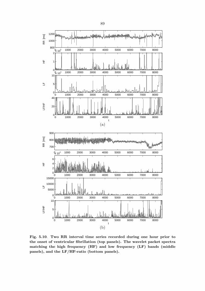
89

0 1000 2000 3000 4000 5000 6000 7000 8000800

1000

1200

RR

[m

s]

0 1000 2000 3000 4000 5000 6000 7000 80000

1

2x 10

5

HF

0 1000 2000 3000 4000 5000 6000 7000 80000

5

10x 10

4

LF

0 1000 2000 3000 4000 5000 6000 7000 80000

20

40

LF/H

F

t

(a)

0 1000 2000 3000 4000 5000 6000 7000 8000

700

800

900

RR

[m

s]

0 1000 2000 3000 4000 5000 6000 7000 80000

2

4

6

x 104

HF

0 1000 2000 3000 4000 5000 6000 7000 80000

5000

10000

15000

LF

0 1000 2000 3000 4000 5000 6000 7000 80000

5

10

LF/H

F

t

(b)

Fig. 5.10. Two RR interval time series recorded during one hour prior to

the onset of ventricular fibrillation (top panels). The wavelet packet spectra

matching the high frequency (HF) and low frequency (LF) bands (middle

panels), and the LF/HF-ratio (bottom panels).

6. Summary and conclusion

Quantifying the variability in cardiovascular signals provides information aboutautonomic neural regulation of the heart and the circulatory system. Neural reg-ulation due to the sympathetic and parasympathetic divisions of the autonomicnervous system involve responses to respiration, blood pressure regulation andthermoregulation. Many cardiovascular diseases, medication and physical andmental stress alter the degree of neural regulation. It is the amount and balanceof the sympathetic and parasympathetic regulations which is often being quanti-fied. Several factors thus have an indirect effect on these signals. Artifacts andseveral types of noise are also contamined together with a useful information. Allthese data can be observed in the dynamics of both heart rate and ventricularrepolarization duration.

The ambulatory measurement setting produces a further demand on the record-ing and analysis of signals. However, there is an increasing need for extending theambulatory recording and increasing the duration of data acquisition. This trendnaturally leads to a greater mass of data and a need for the development of moresophisticated and robust signal analysis schemes.

RR interval recording, which is used to describe heart rate variability (HRV),involves a noninvasive and easy approach to gain information on cardiovascularfunction. Accurate recording equipment has been developed for this technique.The variability in RR intervals is often so large that most of the analysis methodsmay be resolved fairly well in noticeably noisy conditions. Nevertheless, there areimportant factors which should be taken into account when RR interval measure-ment is used. The accuracy of HRV measurement is a consequence of the samplingaccuracy of an ECG and the properties of the method quantifying the signal vari-ability. For example, spectral analysis methods may not fit conditions where sometime domain methods can be used. The reproducibility of the measurement isaffected by the lack of precisely controlled conditions and variation of the resultsthus appear among repeated recordings. This kind of variation is characteristic foran indirect acquisition of information from a biological system. Overall, the varia-tion is an unavoidable condition and has to be kept in mind when interpreting theresults between repeated recordings made for a single person as well as compar-ing the results obtained from different patient sets. RR interval recordings often

91

include abnormal intervals, which may be due to heart rhythm disturbances or er-rors in signal detection of a technical or physiological origin. Time series includingdata points differing from a normal sinus rhythm sometimes carry important in-formation, but may not be, as such, suitable for an analysis performed by all HRVindices. Furthermore, non-periodic changes in RR intervals due to physiologicalresponses can also impair the stationarity of the signal. Several approaches forcorrecting artifacts from time series and eliminating their effect on HRV indiceshave been developed.

The above points also concern ventricular repolarization duration (VRD) mea-surement, which has additional requirements. The detection of the onset of Qwave and the offset of T wave has turned out to be a difficult task due to poorsignal-to-noise ratio. To solve this problem and, when the interest actually lieson the measurement of the ventricular repolarization duration, RTmax interval hasbeen chosen for a QT interval estimate. In addition, VRD time series has a muchlower variability than RR intervals, which places higher requirements on the sam-pling frequency of the ECG. The variability of VRD time series has been morefrequently extracted from an ambulatory ECG with an interpolation procedure toobtain an adequate time resolution for time interval measurement. There is thus aneed for data acquisition equipment, which can collect and store ambulatory ECGwith a higher sampling frequency than ordinary Holter devices do. It was shownby the experiments in this study that VRD variability measurement involve po-tential noise sources and errors, which should be kept in mind during the analysisphase.

An improved accuracy of VRD variability estimation can be attained by themeasurement of action potential duration (APD) variability, which is an invasiveprocedure. However, there may exist technical problems in monophasic action po-tential (MAP) measurements mainly due to poor electrode contact and the effectsof fluctuations in blood pressure and contractility of the ventricle. APD inter-vals showed a low variability compared to RR intervals, which further support therequirements given for the VRD variability estimation. The study of the instan-taneous APD variability related to the short-term RR interval variability in sinusrhythm, indicated that the respiratory vagal modulation of heart rate modify indi-rectly the ventricular repolarization duration. Intrinsic long term fluctuations wereobserved in APD variability, but the constant rate pacing experiment showed thatthe long-term heart rate fluctuation is still the most essential factor determiningthe VRD dynamics in sinus rhythm.

The most simple parameters describing the variability in a time series are statis-tical indices in time domain, which has traditionally been widely used. The indicesreferred in this study as time domain methods contain scarcely any information onperiodic fluctuations, but rather measure the average or maximum amplitude ofthe variability. On the other hand, when the information content of these indicesmay be limited, they suffer less from nonstationarities in a time series.

The periodic fluctuations in cardiovascular variability signals have been ana-lyzed using spectral estimation performed by Fourier and parametric (autoregres-sive, AR) techniques. The main objective has been to decompose the periodicfluctuations due to various sources into well separated components in the power

92

spectrum. Furthermore, some emphasis has been placed on the estimate of vari-ability (power) included in a single component and of the central frequency of thecomponent. The main components in the power spectrum have been linked tothe neural regulation of the heart due to autonomic nervous system through itssympathetic and parasympathetic parts. In this thesis, the stress was on the esti-mation of the power spectrum using an AR model of a time series. An approachfor estimating the powers and the spectra related to components using residuecalculation was also presented.

Observing the evolution of the spectral properties of the signal is of more cur-rent interest. The temporal location of the spectral components has often beenshown to give more information than a single “average” spectrum. Time-frequencymethods include short-time Fourier transform and Wigner distribution, when ap-proaches based on the parametric time series modelling are referred to time-variantspectral analysis methods. The objective has also been to take account existingnonstationarities in time series.

Wavelet transforms are fairly novel approaches in cardiovascular signal analysis,where they may be suitable for processing of nonstationary signals. In this studythe basic theory of wavelet methods was briefly introduced including multiresolu-tion, subband filtering and wavelet packet analysis schemes. The theory related tosignal denoising with several principles for the threshold selection was presented.The methods were then applied to remove simulated noise from ECG. The ex-periments showed that wavelet packet approaches with adaptation by means ofthe optimization of the best tree decomposition structure were not generally moreefficient than the basic wavelet approach. Denoising errors seemed to concen-trate on the high-frequency parts of the ECG when the pure wavelet approachwas employed. Furthermore, the soft thresholding nonlinearity tend to produceproportionally a larger error than the hard thresholding nonlinearity within theQRS-complex.

The motivation of estimating the spectrum of RR interval time series usingwavelet transforms was based on the idea of a more suitable basis function com-pared to Fourier transforms and that any assumptions concerning signal station-arity was not made. In addition, wavelet transforms have flexible resolution prop-erties which means, for example, that they can detect high frequency componentswith a good time resolution. The results show that wavelet transforms were capa-ble to estimate the evolution of the spectrum of RR interval time series obtainedby an ambulatory recording in conjunction with a drug injection and prior to theonset of ventricular fibrillation. In this application wavelet transforms are closelyrelated to time-frequency and time-variant spectral analysis methods.

There is an obvious need of standardization and definition of the measurementand analysis schemes of the cardiovascular variability signals. The meaning of somevariability measures is more complicated than often regarded which sometimesresult in variable and erroneous conclusions. The Task Force report (Task Forceof ESC & NASPE 1996) can be seen as a step along this way, although it containschiefly a report of performed investigations without deeper arguments for methodsand their application.

The development of analysis procedures for cardiovascular variability signals

93

will continue and novel methods will be applied in this field. It is probable thatapproaches for the analysis of nonstationary signals will be more extensively usedin the future. As these signals can only be assumed stationary within some pe-riod, there is also an interest to analyze data obtained under varying conditionslike autonomic function tests. Detecting nonlinearities is also of growing interestas some approaches were reviewed in this thesis. Novel analysis schemes may of-fer additional and valuable information when the characteristics of methods aresufficiently described.

References

Adamson P, Huang M, Vanoli E, Foreman R, Schwartz P & Hull S (1994) Unexpectedinteraction between β-adrenergic blockade and heart rate variability before and aftermyocardial infarction: a longitudinal study in dogs at high and low risk for suddencardiac death. Circulation 90: 976–982.

Akay M (1995) Wavelets in biomedical engineering. Ann Biomed Eng 23: 531–542.

Akay M, Landesberg G, Welkowitz W, Akay YM & Sapoznikov D (1993) Carotid-cardiacinteraction: Heart rate variability during the unblocking of the carotid artery. In:Sideman S & Beyar R (eds) Interactive Phenomena in the Cardiac System. PlenumPress, New York, p 365–372.

Akay M & Mulder E (1996) Examining fetal heart-rate variability using matching pur-suits. IEEE Eng Med Biol 15(5): 64–67.

Akselrod S, Gordon D, Madved J, Snidman N, Shannon D & Cohen R (1985) Hemody-namic regulation: investigation by spectral analysis. Am J Physiol 249: H867–H875.

Babloyantz A & Destexhe A (1988) Is the normal heart a periodic oscillator. Biol Cybern58: 203–211.

Baevskij R, Kirillov O & Kletskin S (1984) Mathematical Analysis of the Changes inCardiac Rhythm During Stress. Nauka, Moscow.

Barbaro V, Bartolini P & Fierli M (1991) New algorithm for the detection of the ECGfiducial point in the averaging technique. Med Biol Eng Comput 29: 129–135.

Basano L, Ottonello P, Poggi A, Adezati L, Semino S, Ubaldi P & Viviani G (1995) Aninstrument for real-time spectral estimation of heart rate variability signal. ComputMethods Programs in Biomed 47: 229–236.

Baselli G & Cerutti S (1985) Identification techniques applied to processing of signalsfrom cardiovascular systems. Med Inf 10(3): 223–235.

Baselli G, Cerutti S, Civardi S, Lombardi F, Malliani A, Merri M, Pagani M & Rizzo G(1987) Heart rate variability signal processing: A quantitative approach as an aid todiagnosis in cardiovascular pathologies. Int J Bio Med Comput 20: 51–70.

Bellavere F (1995) Heart rate variability in patients with diabetes and other noncardio-logical diseases. In: Malik M & Camm A (eds) Heart rate variability. Futura PublishingCompany, Armonk, p 507–516.

95

Bernardi L, Ricordi L, Lazzari P, Solda P, Calciati A, Ferrari M, Vandea I, Finardi G &Frantino P (1992) Impaired circulation modulation of sympathovagal modulation ofsympathovagal activity in diabetes. Circulation 86: 1443–1452.

Berntson G, Quigley J, Jaye F & Boysen S (1990) An approach to artifact identification:Application to heart period data. Psychophysiology 27(5): 586–598.

Bianchi A, Mainardi L, Petrucci E, Signorini M, Mainardi M & Cerutti S (1993) Time-variant power spectrum analysis for the detection of transient episodes in HRV signal.IEEE Trans Biomed Eng BME-40(2): 136–144.

Bigger J, Rolnitzky L, Steinman R & Fleiss J (1994) Predicting mortality after myocardialinfarction from the response of RR variability to antiarrhythmic drug therapy. J AmColl Cardiol 23: 733–740.

Borland (1991) Turbo C++ 3.0 for Windows. Programmer’s Guide. Borland Interna-tional, Inc., Scotts Valley.

Bruce AG & Gao HY (1996) Understanding WaveShrink: Variance and bias estimation.Biometrika 83(4): 727–745.

Calcagnini G, Censi F, Camera A, Lino S & Cerutti S (1996) Interference and phaselocking patterns between low and high frequency rhythms of cardiovascular signals innormal subjects. Proc 18th Annual International Conference of IEEE–EMBS, Ams-terdam.

Casolo G, Balli E, Taddei T, Amuhasi J & Gori C (1989) Decreased spontaneous heartrate variability in congestive heart failure. Am J Cardiol 64: 1162–1167.

Casolo G, Stroder P, Signorini C, Calzolari F, Zucchini M & Balli E (1992) Heart ratevaribility during the acute phase of myocardial infarction. Circulation 85: 2073–2079.

Cerutti S, Bianchi A, Baselli G, Civardi S, Guzzetti S, Malliani A, Pagani A & Pagani M(1989) Compressed spectral arrays for the analysis 24-hr heart rate variability signal.Enhancement of parameters and data reduction. Comput Biomed Res 22: 424–441.

Choi B (1992) ARMA Model Identification. Springer-Verlag, New York.

Clouet J, Fouque J & Postel M (1995) Estimation of local power spectral densities fornon-stationary signals using wavelet transform. Math Comput Simulat 38: 183–188.

Cohen A & Kovacevic J (1996) Wavelets: The mathematical background. Proc IEEE84(4): 514–522.

Cohen L (1989) Time-frequency distributions - a review. Proc IEEE 77(7): 941–981.

Cohen M, Hudson D & Deedwania P (1996) Applying continuous chaotic modeling tocardiac signal analysis. IEEE Eng Med Biol 15(5): 97–102.

Coifman R & Wickerhauser M (1992) Entropy-based algorithms for best basis selection.IEEE Trans Inform Theory 38(2): 713–718.

Coumel P, Fayn J, Maison-Blanche P & Rubel P (1994) Clinical relevance of assessingQT dynamicity in Holter recordings. J Electrocardiology 27S: 62–66.

Daubechies I (1992) Ten Lectures on Wavelets. SIAM, Philadelphia.

Decker J, Schouten E, Klootwijk P, Pool J & Kromhout D (1994) Association betweenQT interval and coronary heart disease in middle-aged and elderly men - The ZutphenStudy. Circulation 90: 779–785.

96

Dimier-David L, Billon N, Costagliola D, Jaillon P & Funck-Brentano C (1994) Repro-ducibility of non-invasive measurement and of short-term variability of blood pressureand heart rate in healthy volunteers. Br J Clin Pharmacol 38: 109–115.

Donoho D (1993) Nonlinear wavelet methods for recovery of signals, densities, and spectrafrom indirect and noisy data. Proc Symp Appl Math 47: 173–205.

Donoho D (1995) De-noising by soft-thresholding. IEEE Trans Inform Theory 41(3):612–627.

Donoho D & Johnstone I (1994) Ideal spatial adaptation by wavelet shrinkage. Biometrika81(3): 425–455.

Donoho D & Johnstone I (1995) Adapting to unknown smoothness via wavelet shrinkage.J Am Statist Assoc 90: 1200–1224.

Eckberg D (1983) Human sinus arrhythmia as an index of vagal cardiac outflow. RespiratEnviron Exercise Physiol 54(4): 961–966.

Extramiana F, Huikuri H, Neyroud N, Koistinen J, Coumel P & Maison-Blanche P(1997) QT rate adaptation: A new index to discriminate patients with and withoutventricular arrhythmias following myocardial infarction (abstract). Circulation 96(8):4014.

Farrell T, Bashir Y, Cripps T, Malik M, Poloniecki J, Bennett E, Ward D & CammA (1991) Risk stratification for arrhythmic events in postinfarction patients based onheart rate variability, ambulatory electrocardiographic variables and the signal aver-aged electrocardiogram. J Am Coll Cardiol 18: 687–697.

Ferrari GD, Mantica M, Vanoli E, Hull S & Schwartz P (1993) Scopolamine increasesvagal tone and vagal reflexes in patients after myocardial infarction. J Am Coll Cardiol22: 1327–1334.

Franz G (1991) Method and theory of monophasic action potential recording. ProgCardiovasc Dis 33: 347–368.

Freeman R, Saul J, Roberts M, Berger R, Broadbridge C & Cohen R (1991) Spectralanalysis of heart rate in diabetic neuropathy. Arch Neurol 48: 185–190.

Friesen G, Jannett T, Jadallah M, Yates S, Quint S & Nagle H (1990) A comparison ofthe noise sensitivity of nine QRS detection algorithms. IEEE Trans Biomed Eng 37:85–98.

Furlan R, Guzzetti S, Crivellaro W, Dassi S, Tinelli M, Baselli G, Cerutti S, LombardiF, Pagani M & Malliani A (1990) Continuous 24-hour assessment of neural regulationof systemic arterial pressure and RR variabilities in ambulant subjects. Circulation81: 537–547.

Furlan R, Piazza S, Dell’Orto S, Gentile E, Cerutti S, Pagani M & Malliani A (1993)Early and late effects of exercise and athletic training on neural mechanisms controllingheart rate. Cardiovascular Research 27: 482–488.

Guzzetti S, Dassi S, Pecis M, Casati R, Masu A, Longoni P, Tinelli M, Cerutti S, PaganiM & Malliani A (1991) Altered pattern of circadian neural control of heart period inmild hypertension. J Hypertens 9: 831–838.

Hainsworth R (1995) The control and physiological importance of heart rate. In: MalikM & Camm A (eds) Heart rate variability. Futura Publishing Company Inc., Armonk,p 3–19.

97

Hamilton P & Tompkins W (1986) Quantitative investigation of QRS detection rulesusing the MIT/BIH arrhythmia database. IEEE Trans Biomed Eng 33(12): 1157–1165.

Hess-Nielsen N & Wickerhauser M (1996) Wavelets and time-frequency analysis. ProcIEEE 84(4): 523–540.

Hlawatsch F & Boudreaux-Bartels G (1992) Linear and quadratic time-frequency signalrepresentations. IEEE Signal Process Mag 9(2): 21–67.

Hoopen MT & Bongaarts J (1969) Probabilistic characterization of R-R intervals. Car-diovasc Res 3: 218–236.

Huikuri H (1997) Abnormal dynamics of ventricular repolarization - a new insight intothe mechanisms of life-threatening ventricular arrhythmias. Eur Heart J 18: 893–895.

Huikuri H, Linnaluoto M, Seppanen T, Airaksinen K, Kessler K, Takkunen J & MyerburgR (1992) Circadian rhythm of heart rate variability in survivors of cardiac arrest. AmJ Cardiol 70: 610–615.

Huikuri H, Seppanen T, Koistinen M, Airaksinen K, Ikaheimo M, Castellanos A & Myer-burg R (1996) Abnormalities in beat-to-beat dynamics of heart rate before the spon-taneous onset of life-threatening ventricular tachyarrhythmias in patients with priormyocardial infarction. Circulation 93: 1836–1844.

Jaffe R, Fung D & Behrman K (1993) Optimal frequency ranges for extracting informa-tion on automatic activity from the heart rate spectrogram. J Auton Nerv Syst 46:37–46.

Janssen M, Swenne C, de Bie J, Rompelman O & van Bemmel J (1993) Methods inheart rate variability analysis: Which tachogram should we choose? Comput MethodsPrograms Biomed 41: 1–8.

Johnsen S & Andersen N (1978) On power estimation in maximum entropy spectralanalysis. Geophysics 43(4): 681–690.

Kamalesh M, Burger A, Kumar S, & Nesto R (1995) Reproducibility of time and fre-quency domain analysis of heart rate variability in patients with chronic stable angina.PACE 18: 1991–1994.

Kamath M & Fallen E (1993) Power spectral analysis of heart rate variability: a nonin-vasive signature of cardiac autonomic function. Crit Rev Biomed Eng 21(3): 245–311.

Kanters J, Holstein-Rathlou NH & Agner E (1994) Lack of evidence for low-dimensionalchaos in heart rate variability. J Cardiovasc Electrophysiol 5: 591–601.

Karrakchou M, Vibe-Rheymer K, Vesin JM, Pruvot E & Kunt M (1996) Improvingcardiovascular monitoring through modern techniques. IEEE Eng Med Biol 15(5):68–78.

Katona P & Jih F (1975) Respiratory sinus arrhythmia: noninvasive measure of parasym-pathetic cardiac control. J Appl Physiol 39(5): 801–805.

Kay S (1988) Modern Spectral Estimation. Theory & Application. Prentice Hall, Engle-wood Cliffs.

Keenan DM (1985) A Tukey nonadditivity-type test for time series nonlinearity.Biometrika 72(1): 39–44.

98

Keselbrener L & Akselrod S (1996) Selective discrete Fourier transform algorithm fortime-frequency analysis: Method and application on simulated and cardiovascular sig-nals. IEEE Trans Biomed Eng 43(8): 789–802.

Khadra L, Maayah T & Dickhaus H (1997) Detecting chaos in HRV signals in humancardiac transplant recipients. Computers and Biomedical Research 30: 188–199.

Kitney R, Fulton T, McDonald A & Linkens D (1985) Transient interactions betweenblood pressure, respiration and heart rate in man. J Biomed Eng 7: 217–224.

Kitney R & Rompelman O (eds) (1987) The Beat-by-Beat Investigation of CardiovascularFunction. Clarendon Press, Oxford.

Kleiger R, Stein P, Bosner M & Rottman J (1992) Time domain measurements of heartrate variability. Ambulatory Electrocardiography 10(3): 487–498.

Kobayashi M & Musha T (1982) 1/f fluctuations of heartbeat period. IEEE TransBiomed Eng 29(6): 456–457.

Koeleman A, van den Akker T, Ros H, Janssen R & Rompelman O (1984) Estimationaccuracy of P wave and QRS complex accurrence times in the ECG: The accuracyfor simplified theoretical and computer simulated waveforms. Signal Processing 7:389–405.

Korhonen I (1997) Methods for the analysis of short-term variability of heart rate andblood pressure in frequency domain. PhD thesis, Tampere University of Technology.

Laguna P, Thakor N, Caminal P, Jane R & Yoon HR (1990) New algorithm for QTinterval analysis in 24-hour Holter ECG: Performance and applications. Med Biol EngComput 28: 67–73.

Lau C & Ward D (1989) QT hysteresis: The effect of an abrupt change in pacing rate. In:Butrous G & Schwartz P (eds) Clinical Aspects of Ventricular Repolarization. FarrandPress, London, p 175–181.

Lee F & Nehorai A (1992) Adaptive power spectrum estimation algorithm for heart ratevariability analysis. Computers in Cardiology, 273–276.

Lippman N, Stein K & Lerman B (1994) Comparison of methods for removal of ectopyin measurement of heart rate variability. Am J Physiol 267(Heart Circ. Physiol. 36):H411 – H418.

Lombardi F, Sandrone G, Mortara A, Rovere ML, Colombo E, Guzzetti S & Malliani A(1992) Circadian variation of spectral indices of heart rate variability after myocardialinfarction. Am Heart J 123: 1521–1529.

Loughlin P (1996) Special issue on time-frequency analysis. Proc IEEE 84(9).

Mainardi L, Bianchi A, Baselli G & Cerutti S (1995) Pole-tracking algorithms for the ex-traction of time-variant heart rate variability spectral parameters. IEEE Trans BiomedEng 42(3): 250–259.

Mainardi L, Bianchi A & Cerutti S (1994) On-line beat-to-beat monitoring of spectralparameters of heart rate variability signal using a pole-tracking algorithm. MethodsInf Med 33: 85–88.

Malik M, Cripps T, Farrell T & Camm J (1989a) Long-term spectral analysis of heart ratevariability - an algorithm based on segmental frequency distributions of beat-to-beatintervals. Int J Biomed Comput 24: 89–110.

99

Malik M, Farrell T & Camm A (1990) Circadian rhythm of heart rate variability withclinical and angiographic variables and late mortality after coronary angiography. AmJ Cardiol 66(12): 1049–1054.

Malik M, Farrell T, Cripps T & Camm A (1989b) Heart rate variability in relation toprognosis after myocardial infarction: Selection of optimal processing techniques. EurHeart J 10(12): 1060–1074.

Malik M, Xia R, Odemuyiwa O, Staunton A, Poloniecki J & Camm A (1993) Influenceof the recognition artefact in automatic analysis of long-term electrocardiograms ontime-domain measurement of heart rate variability. Med Biol Eng Comput 31(5):539–544.

Malliani A, Pagani M, Lombardi F & Cerutti S (1991) Cardiovascular neural regulationexplored in the frequency domain. Circulation 84(2): 482–492.

Malmivuo J & Plonsey R (1995) Bioelectromagnetism. Oxford University Press, NewYork.

Marple S (1987) Digital Spectral Analysis with Applications. Prentice Hall, EnglewoodCliffs.

Merri M (1989) Static and dynamic analyses of ventricular repolarization duration. PhDthesis, University of Rochester, Rochester, New York.

Merri M, Alberti M, Benhorin J & Moss A (1991) Preprocessing of Holter ECGs foranalysis of the dynamic interrelations between heart rate and repolarization durationvariabilities. J Electrocardiology 23S: 157–162.

Merri M, Alberti M & Moss A (1993) Dynamic analysis of ventricular repolarizationduration from 24-hour Holter recordings. IEEE Trans Biomed Eng 40(12): 1219–1225.

Merri M, Benhorin J, Alberti M, Locati E & Moss A (1989) Electrocardiographic quan-titation of ventricular repolarization. Circulation 80: 1301–1308.

Merri M, Farden D, Mottley J & Titlebaum E (1990) Sampling frequency of the electro-cardiogram for spectral analysis of the heart rate variability. IEEE Trans Biomed Eng37(1): 99–106.

Merri M, Moss A, Benhorin J, Locati E, Alberti M & Badini F (1992) Relation betweenventricular repolarization duration and cardiac cycle length during 24-hour Holterrecordings. Circulation 85: 1816–1821.

Misiti M, Misiti Y, Oppenheim G & Poggi JM (1996) Wavelet Toolbox. For Use withMATLAB. Wavelet Toolbox User’s Guide. The MathWorks, Inc., Natick.

Molgaard H, Mickley H, Pless P, Bjerregaard P & Moller M (1993) Effects of metoprololon heart rate variability in survivors of acute myocardial infarction. Am J Cardiol 71:1357–1359.

Moser M, Lehofer M, Sedminek A, Lux M, Zapotoczky HG, Kenner T & Noordegraf A(1994) Heart rate variability as a prognostic tool in cardiology - a contribution to theproblem from the theoretical point of view. Circulation 90(2): 1078–1082.

Mulder L (1992) Measurement and analysis methods of heart rate and respiration for usein applied environments. Biol Psychol 34: 205–236.

Nikias C & Petropulu A (1993) Higher-Order Spectra Analysis: A Nonlinear SignalProcessing Framework. PTR Prentice Hall, Englewood Cliffs.

100

Nollo G, Speranza G, Grasso R, Bonamini R & Antolini R (1990) Dynamic measurementof the QT interval. Computers in Cardiology, 463–466.

Nollo G, Speranza G, Grasso R, Bonamini R, Mangiardi L & Antolini R (1992) Sponta-neous beat-to-beat variability of the ventricular repolarization duration. J Electrocar-diol 25(1): 9–17.

Novak P & Novak V (1993) Time/frequency mapping of the heart rate, blood pressureand respiratory signals. Med Biol Eng Comput 31: 103–110.

Novak V, Novak P, Champlain JD, Blanc AL, Martin R & Nadeau R (1993) Influenceof respiration on heart rate and blood pressure fluctuations. J Appl Physiol 74(2):617–626.

Odemuyiwa O, Malik M, Farrell T, Bashir Y, Poloniecki J & Camm J (1991) Comparisonof the predictive characteristics of heart rate variability index and left ventricularejection fraction for all-cause mortality, arrhythmic events and sudden death afteracute myocardial infarction. Am J Cardiol 68: 434–439.

Oetken G, Parks T & Schuessler H (1979) A computer program for digital interpolatordesign. In: the Digital Signal Processing Committee (ed) Programs for Digital SignalProcessing. IEEE Press, New York, p 8.1.1–8.1.6.

Osborne A & Provenzale A (1989) Finite correlation dimension for stochastic systemswith power-law spectra. Physica D 35: 357–381.

Pagani M, Lombardi F, Guzzetti S, Rimoldi O, Furlan R, Pizzinelli P, Sandrone G, Mal-fatto G, Dell’Orto S, Piccaluga E, Turiel M, Baselli G, Cerutti S & Malliani A (1986)Power spectral analysis of heart rate and arterial pressure as a marker of sympatho-vagal interaction in man and concious dog. Circ Res 59: 178–193.

Pagani M, Lombardi F, Guzzetti S, Rimoldi O, Malfatto G, Cerutti S & Malliani A(1984) Power spectral density of heart rate variability as an index of sympatho-vagalinteraction in normal and hypertensive subjects. J Hypertens 2(suppl. 3): 383–385.

Pagani M, Lucini D, Rimoldi O, Furlan R, Piazza S & Biancardi L (1995) Effects ofphysical and mental exercise on heart rate variability. In: Malik M & Camm A (eds)Heart rate variability. Futura Publishing Company Inc., Armonk, p 245–266.

Pagani M, Malfatto G, Pierini S, Casati R, Masu A, Poli M, Guzzetti F, LombardiF, Cerutti S & Malliani A (1988a) Spectral analysis of heart rate varibility in theassessment of autonomic diabetic neuropathy. J Auton Nerv Syst 23: 143–153.

Pagani M, Somers V, Furlan R, Dell’Orto S, Conway J, Baselli G, Cerutti S, Sleight P& Malliani M (1988b) Changes in autonomic regulation induced by physical trainingin mild hypertension. Hypertension 12: 600–610.

Pahlm O & Sornmo L (1984) Software QRS detection in ambulatory monitoring - areview. Med Biol Eng Comput 22: 289–297.

Peng CK, Mietus J, Hausdorff J, Havlin S, Stanley H & Goldberger A (1993) Long-rangeanticorrelations and non-gaussian behavior of the heartbeat. Phys Rev Lett 70(9):1343–1346.

Pinna G, Maestri R, Cesare AD, Colombo R & Minuco G (1994) The accuracy of power-spectrum analysis of heart-rate variability from annotated RR lists generated by Holtersystems. Physiol Meas 15: 163–179.

101

Pinna G, Maestri R & Sanarico M (1996) Effects of record length selection on the accuracyof spectral estimates of heart rate variability: A simulation study. IEEE Trans BiomedEng 43(7): 754–757.

Pitzalis M, Mastropasqua F, Massari F, Forleo C, Maggio MD, Passantino A, ColomboR, Biase MD & Rizzon P (1996) Short- and long-term reproducibility of time andfrequency domain heart rate variability measurements in normal subjects. CardiovascRes 32: 226–233.

Pola S, Macerata A, Emdin M & Marchesi C (1996) Estimation of the power spectraldensity in nonstationary cardiovascular time series: Assessing the role of the time-frequency representations (TFR). IEEE Trans Biomed Eng 43(1): 46–59.

Pomeranz B, Macaulay R, Caudill M, Kutz I, Adam D, Gordon D, Kilborn K, Barger A,Shannon D, Cohen R & Benson H (1985) Assessment of autonomic function in man byheart rate spectral analysis. Am J Physiol 248(Heart Circ. Physiol. 17): H151–H153.

Porta A, Baselli G, Lombardi F, Malliani A, Greco MD, Ravelli F, Antolini R & NolloG (1996) Performance analysis of the automatic RTapex and RTend measurement.Computers in Cardiology, 533–536.

Priestley M (1981) Spectral Analysis and Time Series. Academic Press Inc., London.

Priestley M (1996) Wavelets and time-dependent spectral analysis. J Time Series Analysis17(1): 85–103.

Proakis J, Rader C, Ling F & Nikias C (1992) Advanced Digital Signal Processing.Macmillan, New York.

Rienzo MD, Castiglioni P, Mancia G, Parati G & Pedotti A (1989) 24 h sequentialspectral analysis of arterial blood pressure and pulse interval in free-moving subjects.IEEE Trans Biomed Eng 36(11): 1066–1075.

Rienzo MD, Mancia G, Parati G, Pedotti A & Zanchetti A (eds) (1993) Blood Pressureand Heart Rate Variability. Computer Analysis and Clinical Applications. IOS Press,Amsterdam.

Rioul O & Vetterli M (1991) Wavelets and signal processing. IEEE Signal Process Mag8(4): 14–38.

Rovere ML, Specchia G, Mortara A & Schwartz P (1988) Baroreflex sensitivity, clinicalcorrelates, and cardiovascular mortality among patients with a first myocardial infarct.Circulation 78: 816–824.

Ruha A, Sallinen S & Nissila S (1997) A real-time microprocessor QRS detector systemwith a 1 ms timing accuracy for the measurement of ambulatory HRV. IEEE TransBiomed Eng 44(3): 159–167.

Sandrone G, Mortara A, Torzillo D, Rovere ML, Malliani A & Lombardi F (1994) Effectsof beta blockers (atenolol or metoprolol) on heart rate variability after acute myocardialinfarction. Am J Cardiol 74: 340–345.

Sapoznikov D, Luria M & Gotsman M (1993) Comparison of different methodoligies ofheart rate variability analysis. Comput Methods Programs Biomed 41: 69–75.

Sapoznikov D, Luria M & Gotsman M (1994) Differentation of periodic from nonperiodiclow-frequency heart rate fluctuations. Comput Biomed Res 27: 199–209.

102

Sapoznikov D, Luria M, Mahler Y & Gotsman M (1992) Computer processing of artifactand arrhythmias in heart rate variability analysis. Comput Methods Programs Biomed39: 75–84.

Saul J, Albrecht P, Berger R & Cohen R (1987) Analysis of long term heart rate variabil-ity: Methods, 1/f scaling and implications. Computers in Cardiology pp. 419–422.

Scott D (1979) On optimal and data-based histograms. Biometrika 66(3): 605–610.

Selman A, McDonald A, Kitney R & Linkens D (1982) The interaction between heartrate and respiration: Part I. Experimental studies in man. Automedica 4: 131–139.

Signorini M, Cerutti S, Guzzetti S & Parola R (1994) Non-linear dynamics of cardiovas-cular variability signals. Methods Inf Med 33: 81–84.

Speranza G, Nollo G, Ravelli F & Antolini R (1993) Beat-to-beat measurement andanalysis of the R-T interval in 24 h ECG Holter recordings. Med Biol Eng Comput31: 487–494.

Stein P, Bosner M, Kleiger R & Conger B (1994) Heart rate variability: A measure ofcardiac autonomic tone. Am Heart J 127(5): 1376–1381.

Stinton P, Tinker J, Vickery J & Vahl S (1972) The scattergram. A new method forcontinuous electrocardiographic monitoring. Cardiovasc Res 6: 598–604.

Strang G & Nguyen T (1996) Wavelets and Filter Banks. Wellesley-Cambridge Press,Wellesley.

Task Force of ESC & NASPE (1996) Heart rate variability. Standards of measurement,physiological interpretation, and clinical use. Task Force of the European Society ofCardiology and the North American Society of Pacing and Electrophysiology. Circu-lation 93(5): 1043–1065.

Thakor N & Sherman D (1995) Wavelet (time-scale) analysis in biomedical signal pro-cessing. In: Bronzino J (ed) The Biomedical Engineering Handbook. CRC Press, Inc.,Boca Raton, p 886–906.

Theiler J, Eubank S, Longtin A, Galdrikian B & Farmer J (1992) Testing for nonlinearityin time series: The method of surrogate data. Physica D 58: 77–94.

Thomas L, Clark K, Mead C, Ripley K & Oliver G (1979) Automated cardiac dysrhyth-mia analysis. Proc IEEE 67(9): 1322–1337.

Tsuji H & Mori H (1994) New analysis of HRV through wavelet transform. InternationalJournal of Human Computer Interaction 6(2): 205–217.

Tsuji H, Venditi F, Manders E, Evans J, Larson M, Feldman C & Levy D (1994) Reducedheart rate variability and mortality risk in an elderly cohort - The Framingham HeartStudy. Circulation 90(2): 878–883.

Unser M & Aldroubi A (1996) A review of wavelets in biomedical application. Proc IEEE84: 626–638.

VanRavenswaaij-Arts C, Kollee L, Hopman J, Stoelinga G & VanGeijn H (1993) Heartrate variability, review. Ann Intern Med 118(6): 436–447.

Wiklund U, Akay M & Niklasson U (1997) Short-term analysis of heart-rate variabilityby adapted wavelet transforms. IEEE Eng Med Biol 16(5): 113–138.

103

Willard K & Connelly D (1992) Nonparametric probability density estimation: Improve-ments to the histogram for laboratory data. Comput Biomed Res 25: 17–28.

Xiong Z, Ramchandran K, Herley C & Orchard M (1997) Flexible tree-structured signalexpansions using time-varying wavelet packets. IEEE Trans Signal Processing 45(2):333–345.

Yamamoto Y, Fortrat JO & Hughson R (1995) On the fractal nature of heart rate vari-ability in humans: Effects of respiratory sinus arrhythmia. Am J Physiol 269(HeartCirc. Physiol. 38): H480–H486.

Yamamoto Y & Hughson R (1993) Extracting fractal components from time series. Phys-ica D 68: 250–264.

Yamamoto Y, Hughson R, Sutton J, Houston C, Cymerman A, Fallen E & Kamath M(1993) Operation everest II: An indication of deterministic chaos in human heart ratevariability at simulated extreme altitude. Biol Cybern 69: 205–212.

Yang F & Liao W (1997) Modeling and decomposition of HRV signals with wavelettransforms. IEEE Eng Med Biol 16(4): 17–22.

Yeragani V, Srinivasan K, Vempati S, Pohl R & Balon R (1993) Fractal dimension ofheart rate time series: An effective measure of autonomic function. J Appl Physiol75(6): 2429–2438.

Ziegler D, Laux G, Dannehl K, Spuler M, Muhlen H, Mayer P & Gries F (1992) As-sessment of cardiovascular autonomic function: Age-related normal ranges and repro-ducibility of spectral analysis, vector analysis, and standard tests of heart rate variationand blood pressure responses. Diabet Med 9: 166–175.

Ziemer R & Tranter W (1990) Principles of Communications. Systems, Modulation andNoise. Houghton Mifflin Company, Boston.

Zuanetti G, Latini R, Neilson J, Schwartz P, Ewing D & the Antiarrhythmic drug evalu-ation group (ADEG) (1991) Heart rate variability in patients with ventricular arrhyth-mias: Effect of antiarrhythmic drugs. J Am Coll Cardiol 17: 604–612.

Ori Z, Monir G, Weiss J, Sayhouni X & Singer D (1992) Heart rate variability. Frequencydomain analysis. Ambulatory Electrocardiography 10(3): 499–537.