Characteristics of the large-scale circulation changes during the sudden onset of the fall transition season

INTERNATIONAL JOURNAL OF CLIMATOLOGY

Int. J. Climatol. 20: 397–415 (2000)

CHARACTERISTICS OF THE LARGE-SCALE CIRCULATIONCHANGES DURING THE SUDDEN ONSET OF THE FALL

TRANSITION SEASONLINDA M. KELLER* and DAVID D. HOUGHTON

Department of Atmospheric and Oceanic Sciences, Uni6ersity of Wisconsin-Madison, Madison, WI, USA

Recei6ed 22 December 1998Re6ised 15 June 1999

Accepted 25 June 1999

ABSTRACT

The characteristics of large-scale circulation changes manifest in the abrupt onset of the fall transition season areanalysed for the Northern Hemisphere extratropical region. Ten years of daily observational data from the EuropeanCentre for Medium Range Weather Forecasts (ECMWF) global model initialization analyses are examined using thevertically integrated total kinetic energy (TKE) as the primary descriptor for circulation intensity. The time series dataare bandpass filtered to examine subsets of frequencies representing specific atmospheric time scales, i.e. thelow-frequency tropical forced oscillations (29.9–59.9 days), the intermediate-frequency oscillations related to non-lin-ear processes such as weather regimes (10.0–29.7 days) and the high-frequency extratropical synoptic scale (2.5–6.5days). Times when significant increases in kinetic energy (KE) variability occurred in the area-weighted hemispheric-mean time series for each bandpass were determined, and the onset date for each year and for each bandpass periodwas designated as the first significant increase in KE variability during the 1 August–30 November time period.

Statistically significant abrupt onset events are found, with the majority occurring in August, September andOctober. The mean onset times vary from 3 October for the 29.9–59.9-day bandpass period to 30 August for the2.5–6.5-day bandpass period. Composites with respect to the onset time show robust features of the abrupt onsetevent in both the hemispheric-mean time series and the spatial patterns of KE variability.

Centres of maximum change in the magnitude of KE variability are in the western and central Pacific and theAtlantic Ocean sectors coincident with the areas of jet stream maxima. Separate analyses for onset characteristics forarea-mean KE time series for the Pacific and Atlantic Ocean areas show that there is little correlation between Pacificand Atlantic onset times for the 29.9–59.9-day bandpass period. However, for the 10.0–29.7-day bandpass period theAtlantic onset times tend to lead the Pacific onset times, while for the 2.5–6.5-day bandpass period the Pacific regiononset times tend to occur prior to the Atlantic onset times. Copyright © 2000 Royal Meteorological Society.

KEY WORDS: Northern Hemisphere; time series analysis; kinetic energy; transition season circulation

1. INTRODUCTION

The inherent non-linear nature of the atmosphere is manifest in interactions and fluctuations on a widerange of space and time scales. In the case of extratropical seasonal change considerations, even thoughthe basic forcing is the smoothly varying input from solar radiation at the top of the atmosphere, thelarge-scale flow variations in the middle latitudes include fluctuations on many time scales.

The episodic or abrupt change of extratropical circulation patterns is one of the more dramaticcharacterizations of the non-linear system. Abrupt changes in circulation patterns have been documentedin many observational studies (e.g. Namias, 1952, 1988, 1990; Mo and Ghil, 1988; Zeng et al., 1994), butthe overall characterization, let alone understanding, of abrupt changes remains unresolved. Some of theobservational evidence has been regional (e.g. Yeh et al., 1959; Zeng et al., 1988; Matsumoto, 1992), basedon very limited global parameters (Wahl, 1972), or focused more on the extreme season (winter) and

* Correspondence to: Department of Atmospheric and Oceanic Sciences, University of Wisconsin-Madison, 1225 West DaytonStreet, Madison, WI 53706, USA.

Copyright © 2000 Royal Meteorological Society

L.M. KELLER AND D.D. HOUGHTON398

weather regime shifts (Mo and Ghil, 1988; Dole, 1989; Dole and Black, 1990). In studies related to theAsian monsoon, Tao and Chen (1987) examined onset times for abrupt changes in the Asian monsoon,and Matsumoto (1992) documented nearly simultaneous changes in circulation parameters over largeregions in the monsoon area. Wang and Xu (1997) found statistically significant intraseasonal monsoonevents occurred regularly at specific times from August through to October. Numerical modellingsimulations have captured examples of abrupt shifts or related multiple-equilibria characteristics of theatmospheric circulation (Otto-Bliesner, 1980; Mo and Ghil, 1988; Zeng et al., 1988; Hansen and Sutera,1992).

Understanding the processes for abrupt changes in the transition seasons involves non-linear dynamicstheory for the atmospheric global circulation (Ghil, 1987). Lorenz (1990) sees the transition seasons asmodulators or bridges between extreme seasons. The new heating distribution that arrives with atransition season breaks up those existing circulation patterns which are incompatible with it. In turn, asomewhat randomly chosen circulation pattern would be in place when the next extreme season begins.Abrupt changes on a large spatial scale in the extratropics could involve instability in global-scale wavemodes of the type discussed by Borges and Hartmann (1992), tropical forcing (Fleming et al., 1987), orsystematic feedback loops with transient disturbances. Fleming et al. (1987) also found asymmetries in thelatitude of the zonally averaged jet flow in the Northern Hemisphere between the spring and fall seasons,but their analysis used 5-day and monthly means which precluded a description of abrupt shifts in suchchanges. Basic theory for weather regimes including the role of transient eddies (e.g. Mo and Ghil, 1988;Lau and Peng, 1992; Molteni and Palmer, 1993; Reinhold and Yang, 1993; Sheng and Derome, 1993;Orlanski, 1998) could provide some clues to the dynamics and the timing of the seasonal abrupt changes.

The purpose of this study is to describe changes in the characteristics of the Northern Hemispherecirculation for the fall transition season, with a focus on examples of the more abrupt aspects. Specifically,the sudden onset of larger variability of hemispheric- and regional-mean kinetic energy (KE) associatedwith the transition from summer to winter conditions is examined. A regional analysis of associated KEvariability changes is carried out to provide some initial suggestions for the dynamical underpinning forthis sudden onset characteristic. An understanding of such characteristics of the transition seasons isessential for improving long-range and seasonal prediction. In addition, the atmospheric forcing ofvariability in the oceans relates directly to the integral effects of the atmosphere, which include lengths ofthe seasons.

2. DATA

The primary data are observations of u and 6 wind components obtained from the 6-h initializationanalysis data sets for the European Centre for Medium Range Weather Forecasts (ECMWF) globalnumerical prediction model which have been interpolated to the National Center for AtmosphericResearch Community Climate Model 2 (CCM2) grid (a mesh of approximately 2.8° spacing in bothlatitude and longitude) on pressure coordinates (Trenberth, 1992). The data from 10 years of this specialdata set (1987–1996) were used. Daily values were obtained by averaging the 6-h data. Only NorthernHemisphere data north of 18°N are considered.

The vertically integrated total kinetic energy (TKE) of the atmosphere was calculated from the u and6 components at each pressure level and this was used as the descriptor for the intensity of theatmospheric circulation. This parameter has horizontal spatial variations that describe both the regionaland the large-scale structure of the flow, and relates directly to the dynamics and stability characteristicsof the atmospheric system. It is directly associated with the development of synoptic scale eddies in thatthe advection of large amounts of KE contributes to the growth of the eddies until baroclinic processes,in the form of conversion of available potential energy, become important (Sechrist and Rudy, 1969).Daily means of area-weighted vertically integrated TKE averaged over the Northern Hemisphere (northof 18°N) are used first for the time series analyses. Additional analyses are performed for two limitedregions—the western Pacific Ocean and eastern North America/western Atlantic Ocean—which are

Copyright © 2000 Royal Meteorological Society Int. J. Climatol. 20: 397–415 (2000)

FALL SEASON CIRCULATION CHANGES 399

Figure 1. Location of the hemispheric and regional domains. The hemispheric domain (the entire domain shown) is located between18°N and 80°N (the 20°N, 40°N, 60°N and 80°N latitude lines are shown). The Pacific domain is designated as P and the Atlantic

domain as A

centres of action for both mean jet stream flow and flow variability. Figure 1 shows the location of thehemispheric and regional domains.

The time series of daily hemispheric-mean (north of 18°N) TKE has a strong annual cycle as shown inthe 10-year (1987–1996) climatological mean (Figure 2). In order to conduct time series analyses, it wasnecessary to eliminate this signal. Bandpass filters (Raymond, 1988) were applied to the 10-year time

Figure 2. Annual cycle of daily values for the 10-year mean of area-weighted vertically-integrated TKE for the NorthernHemisphere north of 18°N. Units: 105 J m−2



series after the long term (10-year) mean had been removed. The bandpass filter is a high-orderimplicit low-pass tangent filter. A tangent filter is a recursive filter which features a flat amplituderesponse with a sharp curve as it approaches the cutoff frequency. The response of this filter mini-mizes the possibility of any overshooting or Gibbs effect. Three frequency ranges were chosen torepresent shorter time scale dynamical processes. The selected frequency bands were: 29.9–59.9-dayperiod to represent the low-frequency impacts of the tropical 40–50-day oscillation found by Maddenand Julian (1971); 10.0–29.7-day period to characterize the intermediate-frequency variability associ-ated with large-scale non-linear processes such as weather regimes (Mo and Ghil, 1988); and the2.5–6.5-day period to represent high-frequency synoptic scale activity. The bandpass filters were ap-plied to the entire 10-year daily time series, and then the period between 1 August and 30 Novemberfor each year was examined in more detail.

3. CLIMATOLOGY OF THE FALL TRANSITION SEASON

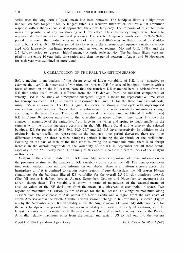
Before moving to an analysis of the abrupt onset of larger variability of KE, it is instructive toexamine the overall characteristics of variations in transient KE for selected bandpass intervals with afocus of attention on the fall season. Note that the transient KE examined here is derived from theKE time series itself, which is different from the KE derived from the transient components ofvelocity used in the study of atmospheric energetics. Figure 3 shows the representative time seriesfor hemispheric-mean TKE, the overall intraseasonal KE, and KE for the three bandpass intervals,using 1995 as an example. The TKE (Figure 3a) shows the strong annual cycle with superimposedsmaller time scale features. Notice that the subseasonal time scale variability magnitudes changeaccording to the time of year. The overall intraseasonal time scale bandpass filtered (2.5–89.1 days)KE in Figure 3b isolates more clearly the variability on many different time scales. It shows thechanges in magnitude of the variability, from large in the winter and spring to much smaller in thesummer with the abrupt increases occurring in the fall. Figure 3c, d and e display the selectedbandpass KE for periods of 29.9–59.9, 10.0–29.7 and 2.5–6.5 days, respectively. In addition to theobviously shorter oscillations represented as the bandpass time period decreases, there are otherdifferences among the three selected bandpass periods including the amplitude of the oscillations.Focusing on the part of each of the time series following the summer minimum, there is an abruptincrease in the overall magnitude of the variability of the KE in September for all three bands,especially in the 2.5–6.5-day band. The timing of this abrupt increase is a central focus of the analysisin this paper.

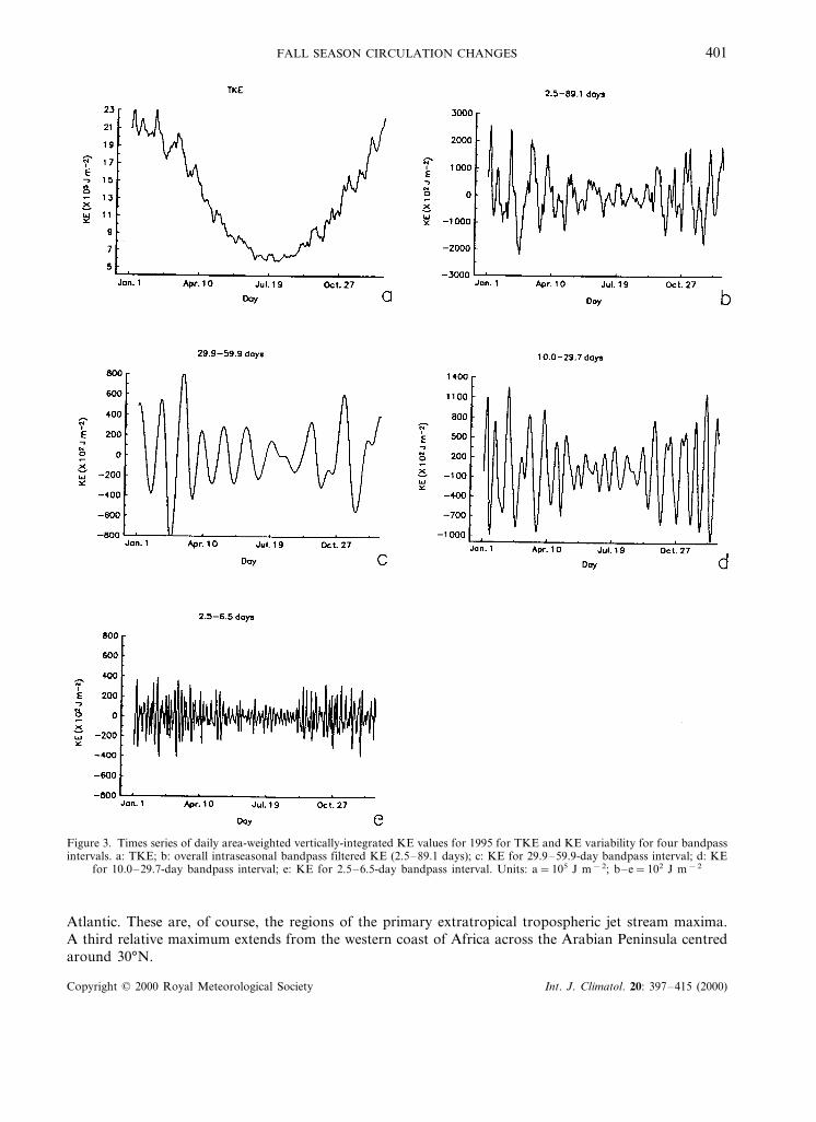
Analysis of the spatial distribution of KE variability provides important additional information onthe processes relating to the changes in KE variability occurring in the fall. The hemispheric-meantime series analysis does not give information on whether there is a uniform increase across thehemisphere or if it is confined to certain active regions. Figure 4a displays the fall season 10-yearclimatology for the bandpass filtered KE variability for the overall 2.5–89.1-day bandpass interval.(The fall season is defined here as August, September, October and November to encompass theabrupt change dates.) The variability is shown in terms of magnitudes of the seasonal-means ofabsolute values of the KE deviations from the mean state observed at each point in space. Tworegions of maximum KE variability are observed for the fall season: an elongated maximum along�45°N from the east coast of Asia across the North Pacific and a region from the east coast ofNorth America across the North Atlantic. Overall seasonal change in KE variability is shown (Figure4b) by the November mean KE variability minus the August mean KE variability difference field forthe same bandpass time period. The changes in variability are positive at nearly all locations, with thelargest increases in KE variability off the east coast of Asia and extending across most of the Pacific.A smaller relative maximum exists from the central and eastern US to well out into the western



Figure 3. Times series of daily area-weighted vertically-integrated KE values for 1995 for TKE and KE variability for four bandpassintervals. a: TKE; b: overall intraseasonal bandpass filtered KE (2.5–89.1 days); c: KE for 29.9–59.9-day bandpass interval; d: KE

for 10.0–29.7-day bandpass interval; e: KE for 2.5–6.5-day bandpass interval. Units: a=105 J m−2; b–e=102 J m−2

Atlantic. These are, of course, the regions of the primary extratropical tropospheric jet stream maxima.A third relative maximum extends from the western coast of Africa across the Arabian Peninsula centredaround 30°N.



Figure 4. Fall season (August, September, October, November) overall intraseasonal bandpass filtered KE variability (2.5–89.1-dayperiod). a: Seasonal means of absolute values of KE deviations from the mean state at each grid point; b: November mean KEvariability minus August mean KE variability difference field. Units: 2×105 J m−2. The 30°N and 60°N latitude lines are shown

4. ANALYSIS METHOD

The seasonal-mean spatial fields show the background characteristics for the seasonal variability andchanges in variability, but they do not provide information regarding the details of the changes associatedwith the abrupt increase events in KE variability, as seen in the area-mean KE time series. It is necessaryto identify the times of the abrupt increase of area-mean KE variability for each bandpass period and foreach year, in order to provide a reference for composites to highlight the associated changes in the KEand other aspects of the circulation during the periods of rapid change. Such composites aid in theisolation of the physical processes associated with rapid changes in variability, such as instability andnon-linear feedback processes.

For this study, the time of the abrupt onset of KE variability increases for each year is defined as theday when the bandpassed area-mean KE time series curve crosses the zero line closest to the firstsignificant overall increase in the magnitude of KE variability during the period 1 August–30 November.Note that all of the bandpass filtered KE time series oscillate about zero. The determination of the abruptonset time requires a procedure that will identify and quantify the significant increases in the magnitudeof KE variability. As a first step, the autocorrelation coefficients were calculated for each of the bandpassfiltered KE time series. This calculation was performed in order to determine whether there was a lag timebeyond which the time series did not show a great amount of persistence and could be considered fairlyindependent. With complete correlation represented by the autocorrelation coefficient equal to 1, the lagtime where the autocorrelation coefficient was less than 0.2 was chosen to represent the length of timeneeded between observations to assume independence. The lag times were determined to be 7 days, 17days and 43 days for the 2.5–6.5, 10.0–29.7 and 29.9–59.9-day bandpass periods, respectively. Thevariance was calculated for periods of 30 days prior to a break period equal to the lag time determinedabove and 30 days following the break period for each day in the 10-year series (60 days prior to andfollowing the break period was used for the 29.9–59.9-day bandpass period in order to include more thanone complete oscillation). The 30 (60) day averaging time was chosen in order to focus on themore-sustained and larger time scale changes within a season. The variance for the first 30 (60) day periodwas subtracted from the variance for the second 30 (60) day period for each reference day (defined as themiddle day of the break period) to give a daily time series for the 30 (60) day variance change with time.For local maxima analysis, the variance difference time series itself was smoothed using an 11-day running



mean (3-day running mean for the 2.5–6.5-day bandpass period) in order to eliminate some of the smallertime scale features in the time series. The smoothed difference time series was then examined for localmaxima in the 1 August–30 November time frame. Only maxima indicating an increase in variability overtime were considered, because this study was interested in the fall increase in KE activity.

In order to determine whether the local maxima represent times of significant KE variability change, aone-tailed F-ratio test was performed on the unsmoothed variance for the 30-day periods prior to andfollowing each break period, centred on the local maxima in the August–November time segment (60days prior to and following was used for the 29.9–59.9-day bandpass period). The F-ratio test examineswhether two sets of data have significantly different variances by calculating the ratio of the variances(Press et al., 1992). A 1% significance level was chosen to determine whether the change in variability wassignificant. Different F-ratios were used for the 30- and 60-day periods for the 1% significance level.

For time series composites, it is necessary to have uniformity in the specification of abrupt change andonset times in the oscillating time series. The time of possible abrupt change was prescribed to be at thepoint (in whole days) at which the original (unsmoothed) bandpassed time series curve crosses the zeroline which is closest to the times identified above. While there can be more than one significant KEvariability magnitude increase during the August–November time period, only the first significantincrease is chosen for the onset time. All years and all bandpass periods were found to have an onset timefor hemispheric-mean KE that satisfied the significance test.

In summary, the specific process for determining onset times is as follows:

(i) Construct the daily time series for the change in variance from the 30-day period prior to the breakperiod to the 30-day period following the break period for each day in the time series (use 60 daysfor the 29.9–59.9-day bandpassed time series).

(ii) Apply an 11-day running mean (3-day running mean for the 2.5–6.5-day bandpass period) to thevariance change time series, in order to eliminate some of the smaller time scale variability.

(iii) Determine the date of each local maximum between 1 August and 30 November in the smoothedvariance-change time series.

(iv) For the local maxima, determine whether the variance of the unsmoothed time series is significant atthe 1% level in accordance with the F-ratio test.

(v) For each day that is significant from (iv) above, find the nearest day where the hemispheric-mean KEtime series crosses the zero line. These are the abrupt change dates.

(vi) Select the first of the abrupt change dates in each year after 1 August as the onset time.

5. RESULTS

5.1. Onset times

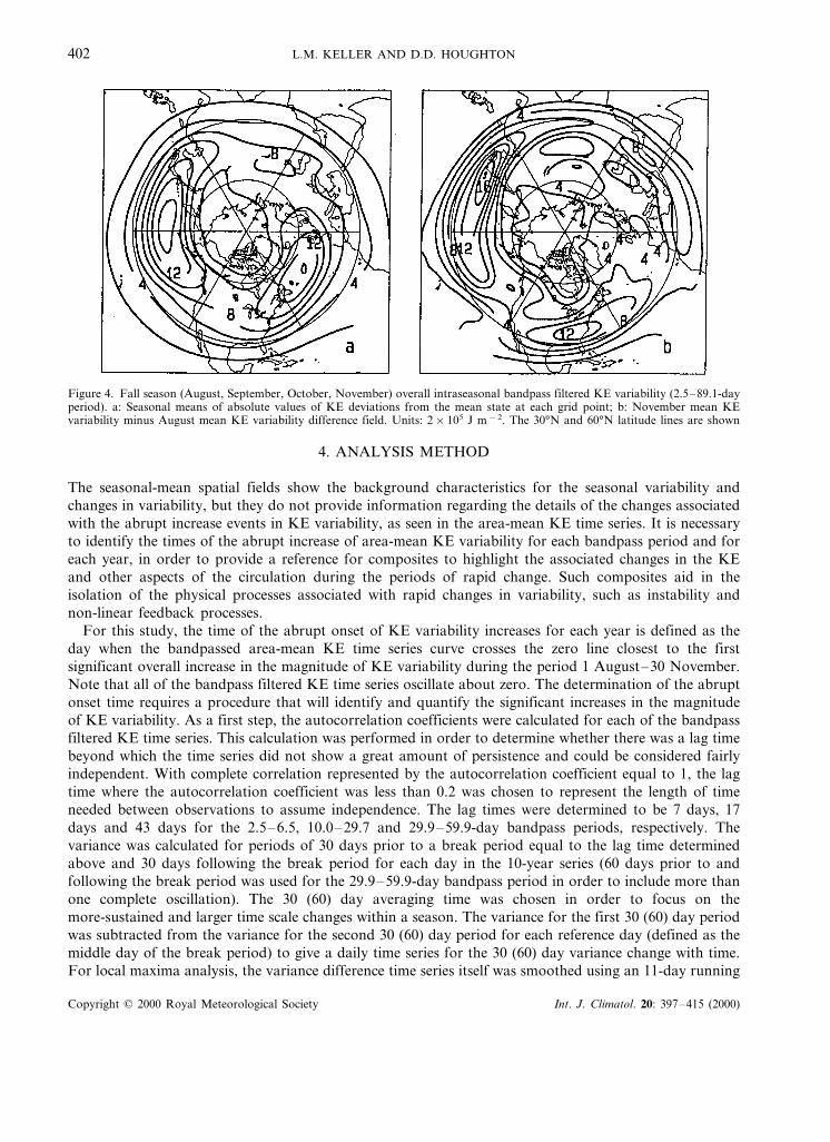
A comparison of onset times by frequency band shows that the bands have systematically differentonset times during the fall period (Figure 5, Table I). For the bandpass time period (29.9–59.9 days)which corresponds to a dominant tropical oscillation, the average onset time is 3 October. Four of theonset times occur in either November or December (Figure 6) and are associated with 4 of the 5 El Ninoyears during the period of study (1987, 1991, 1992, 1993 and 1994 as defined by Goddard and Graham(1997)). Three of the years have more than one significant increase in KE variability magnitude, indicatingthat the initial increase in KE variability is not large enough to reach winter levels, allowing for additionalsignificant variability increases.

The bandpass time period (10.0–29.7 days), which includes weather regimes, has an average onset timearound 28 September (Table I, Figure 5). This is slightly earlier than the average time for the 29.9–59.9day bandpass period. The onset times for the El Nino years tend to be later, but the relationship is notas clear as that observed for the 29.9–59.9-day bandpass period discussed above. Only 2 of the years havemore than one significant increase in KE variability magnitude.



Figure 5. Onset time distributions for the 10-year period for the three bandpass intervals: 29.9–59.9, 10.0–29.7 and 2.5–6.5 days

The synoptic scale frequency band (2.5–6.5-day bandpass period) shows even earlier onset times thanthe other two bands previously discussed (Figure 5, Table I). The average onset time is around 30 August,about a full month earlier than that for the 10.0–29.7-day bandpass period. The onset times are earlierfor El Nino years. Nine of the 10 years in this study have multiple significant increases in the magnitude

Table I. Hemispheric onset times for three bandpass periods

Bandpass periods (days)Year

29.9–59.9 10.0–29.7 2.5–6.5

August 291987 October 29December 171988 August 19 October 7 September 51989 September 18 August 20 September 10

August 20September 4October 151990August 181991 November 6 October 2August 14October 21992 November 14

1993 August 18 September 27 August 111994 November 21 October 13 August 4

September 5September 8September 51995October 30October 11996 October 21

September 28October 3Mean August 30



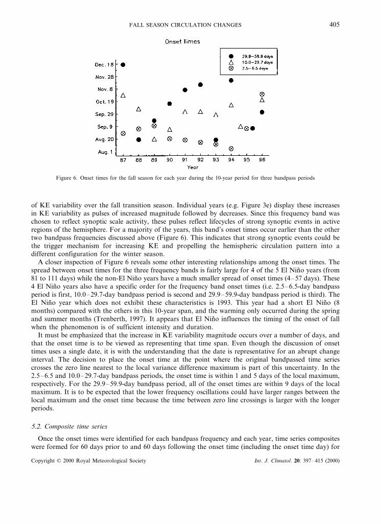
Figure 6. Onset times for the fall season for each year during the 10-year period for three bandpass periods

of KE variability over the fall transition season. Individual years (e.g. Figure 3e) display these increasesin KE variability as pulses of increased magnitude followed by decreases. Since this frequency band waschosen to reflect synoptic scale activity, these pulses reflect lifecycles of strong synoptic events in activeregions of the hemisphere. For a majority of the years, this band’s onset times occur earlier than the othertwo bandpass frequencies discussed above (Figure 6). This indicates that strong synoptic events could bethe trigger mechanism for increasing KE and propelling the hemispheric circulation pattern into adifferent configuration for the winter season.

A closer inspection of Figure 6 reveals some other interesting relationships among the onset times. Thespread between onset times for the three frequency bands is fairly large for 4 of the 5 El Nino years (from81 to 111 days) while the non-El Nino years have a much smaller spread of onset times (4–57 days). These4 El Nino years also have a specific order for the frequency band onset times (i.e. 2.5–6.5-day bandpassperiod is first, 10.0–29.7-day bandpass period is second and 29.9–59.9-day bandpass period is third). TheEl Nino year which does not exhibit these characteristics is 1993. This year had a short El Nino (8months) compared with the others in this 10-year span, and the warming only occurred during the springand summer months (Trenberth, 1997). It appears that El Nino influences the timing of the onset of fallwhen the phenomenon is of sufficient intensity and duration.

It must be emphasized that the increase in KE variability magnitude occurs over a number of days, andthat the onset time is to be viewed as representing that time span. Even though the discussion of onsettimes uses a single date, it is with the understanding that the date is representative for an abrupt changeinterval. The decision to place the onset time at the point where the original bandpassed time seriescrosses the zero line nearest to the local variance difference maximum is part of this uncertainty. In the2.5–6.5 and 10.0–29.7-day bandpass periods, the onset time is within 1 and 5 days of the local maximum,respectively. For the 29.9–59.9-day bandpass period, all of the onset times are within 9 days of the localmaximum. It is to be expected that the lower frequency oscillations could have larger ranges between thelocal maximum and the onset time because the time between zero line crossings is larger with the longerperiods.

5.2. Composite time series

Once the onset times were identified for each bandpass frequency and each year, time series compositeswere formed for 60 days prior to and 60 days following the onset time (including the onset time day) for



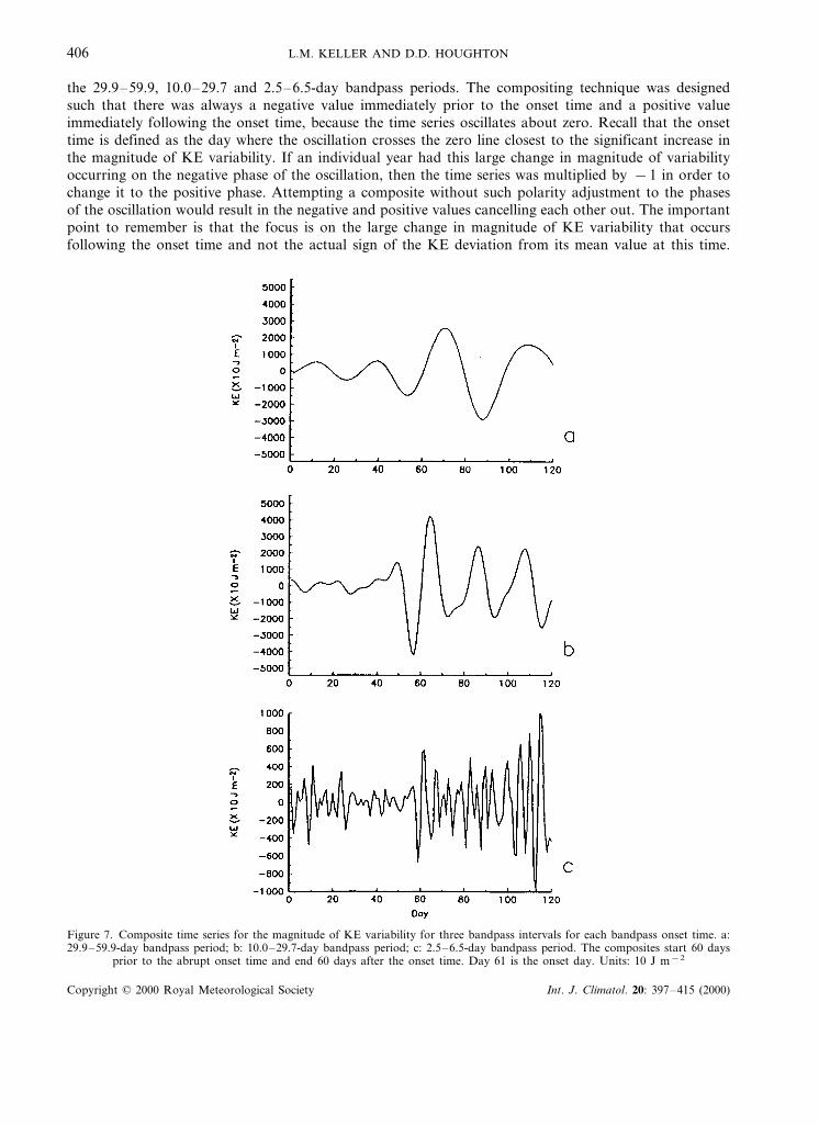
the 29.9–59.9, 10.0–29.7 and 2.5–6.5-day bandpass periods. The compositing technique was designedsuch that there was always a negative value immediately prior to the onset time and a positive valueimmediately following the onset time, because the time series oscillates about zero. Recall that the onsettime is defined as the day where the oscillation crosses the zero line closest to the significant increase inthe magnitude of KE variability. If an individual year had this large change in magnitude of variabilityoccurring on the negative phase of the oscillation, then the time series was multiplied by −1 in order tochange it to the positive phase. Attempting a composite without such polarity adjustment to the phasesof the oscillation would result in the negative and positive values cancelling each other out. The importantpoint to remember is that the focus is on the large change in magnitude of KE variability that occursfollowing the onset time and not the actual sign of the KE deviation from its mean value at this time.

Figure 7. Composite time series for the magnitude of KE variability for three bandpass intervals for each bandpass onset time. a:29.9–59.9-day bandpass period; b: 10.0–29.7-day bandpass period; c: 2.5–6.5-day bandpass period. The composites start 60 days

prior to the abrupt onset time and end 60 days after the onset time. Day 61 is the onset day. Units: 10 J m−2



All three composites shown in Figure 7 show small oscillations prior to the onset time (specified as day61) and a sudden increase in magnitude after the onset time, with a tendency for some decreases later onbecause of the interference and/or cancellation effects arising from a lack of phase correlation. Theoscillations after the onset time are at least twice as large as those prior to the onset time.

5.3. Hemispheric composites

Spatial KE variability–magnitude pattern composites were constructed to provide information onwhether the entire hemisphere is behaving uniformly or whether specific regions are driving the wholesystem during abrupt onset events. Composites are formed using the absolute values of the KE variabilityderived from the bandpass filtering process at each point in space. For the 10.0–29.7-day and 2.5–6.5-daybandpass periods, 30-day averages were computed for the period immediately prior to the abrupt onsetperiod and for the 30 day period starting with the abrupt onset day. For the 29.9–59.9-day bandpassperiod, 60 days were used for the averages instead of 30 days.

5.3.1. 29.9–59.9-day bandpass period. Figure 8a displays the difference field of KE variability magni-tude for the change from 60 days prior to 60 days following for the 29.9–59.9-day bandpass period. Themean hemispheric onset time for this bandpass period is 3 October. Substantial increases in magnitudeoccur off the east coast of Asia, extending across the central Pacific. Other increases are found over thenortheastern US and over the western and eastern areas of the North Atlantic. These differences representnot only an increase in magnitude but an extension of the maximum area in the Pacific, westward intoAsia and eastward into the eastern Pacific. The Atlantic area has the same pattern of western extensioninto the eastern US and eastward into Scandinavia. There is also an increase in variability across theMiddle East to south of the Caspian Sea.

The F-ratio test can be applied to the time series at each grid point to determine which areas of thespatial composites have significant increases in KE variability from prior to following the onset times andhow the ‘local’ onset time corresponds to the hemispheric-mean onset time. The areas that are notsignificant either do not have abrupt onset times or change at a different time than the hemispheric timeseries. For the 29.9–59.9-day bandpass period, the variance increases across the onset time are significantat the 1% level over a large part of the hemisphere. Exceptions are narrow bands stretching across Korea,northern Japan, and out into the Pacific Ocean to 150°W centred around 55°N and a band centredaround 45°N which extends from the Mediterranean across the Middle East to about 90°E. A small areawhere the variance difference is not significant at the hemispheric onset time is also found in the westernAtlantic Ocean and around Scandinavia.

Figure 8b shows the difference field of KE variability for the overall intraseasonal 2.5–89.1-daybandpass period, composited using the 29.9–59.9-day bandpass interval onset times. Comparison withFigure 8a indicates that the overall intraseasonal changes over the onset time have a maximum farthernorth and east in the Pacific than that for the 29.9–59.9-day bandpass period composite alone. In theAtlantic, the overall change maximum is farther south along the east coast of the US. About one-thirdof the overall intraseasonal change in KE variability is accounted for by the 29.9–59.9-day bandpassinterval.

5.3.2. 10.0–29.7-day bandpass period. The difference field of KE variability for the 10.0–29.7-daybandpass period is presented in Figure 8c for the 30 days prior to and following the abrupt onset timesfor this bandpass interval. The mean onset time for this bandpass period is 28 September. The increasesin the magnitude of the variability are concentrated in the central and eastern Pacific. Smaller increasesoccur over central North America and the western North Atlantic, as well as into the British Isles. (Overthe entire period, the largest KE variability already extends from Asia across the entire Pacific and fromthe eastern US to Scandinavia, so the increase in variability represents an intensification of the patternrather than a shift in position.) The maximum KE variability in the Pacific is centred farther north andeast than in the 29.9–59.9-day bandpass period.



Figure 8. Difference fields of composites of the magnitude of the absolute values of KE variability from prior to following eachbandpass onset time for the four bandpass intervals. a: 29.9–59.9-day bandpass period (60 days prior to and following); b: 2.5–89.1day bandpass period (60 days prior to and following) using the onset times from the 29.9–59.9-day bandpass period; c:10.0–29.7-day bandpass period (30 days prior to and following); d: 2.5–89.1-day bandpass period (30 days prior to and following)using the onset times from the 10.0–29.7-day bandpass period; e: 2.5–6.5-day bandpass period (30 days prior to and following); f:2.5–89.1-day bandpass period (30 days prior to and following) using the onset times from the 2.5–6.5-day bandpass period. Units:

a, c and e=5×104 J m−2; b, d and f=10×104 J m−2. The 30°N and 60°N latitude lines are shown

The F-ratio results for the 10.0–29.7-day bandpass period do not show the extensive areas ofsignificant increases discussed for the 29.9–59.9-day bandpass period. Instead, the areas are morelocalized in specific regions. In the Pacific Ocean, significant increases extend out from Asia, south of



Japan, and in the eastern central North Pacific. In North America, the area of significant increasesextends from the west to the east coasts of the US and over eastern Canada. Across the Atlantic region,the area of significant increase lies between 30°N and 45°N. This area continues across northern Africaand south of the Caspian Sea. Another area of significant increase lies across Scandinavia into northernEurope.

The difference field of KE variability for the overall 2.5–89.1-day bandpass period composited usingthe 10.0–29.7-day bandpass interval onset times (Figure 8d) has the main increase in the magnitude of thevariability centred further west in the North Pacific than is the case for the 10.0–29.7-day bandpassperiod composite. The eastern area of North America and an area south of the Canadian MaritimeProvinces in the Atlantic have smaller increases in magnitude. As with the 10.0–29.7-day bandpass periodcomposite, these increases in magnitude are mainly a strengthening of the basic pattern rather thanchanges in position. A comparison with Figure 8c amplitudes shows that over half of the overallintraseasonal change in KE variability is accounted for by the 10.0–29.7-day bandpass interval.

5.3.3. 2.5–6.5-day bandpass period. The difference field of KE variability for the 2.5–6.5-day bandpassperiod is displayed in Figure 8e. The onset times are earlier, with a mean onset time of 30 August. Thelargest increases in the magnitude of the variability are in an area that extends from the east coast of Asiaacross the Pacific and into the northwestern regions of North America. Once again, this is mainly anincrease in intensity rather than a change of position. A region of smaller increases in the magnitude ofthe variability of KE for the North Atlantic is positioned just south of Greenland. The areas of maximumincrease are, in general, positioned farther north than was observed for the 29.9–59.9 and 10.0–29.7-daybandpass periods.

The F-ratio test shows areas of significant increases across the northwestern and central Pacific, theeastern coast of North America extending across Greenland, and across Africa centred around 35°N.Other areas of significant increase are located in northwestern North America and south of the CaspianSea eastward.

Figure 8f shows the difference field of KE variability for the overall intraseasonal (2.5–89.1 days)bandpass period composited using the 2.5–6.5-day bandpass interval onset times. The largest increases inmagnitude of the KE variability extend across the Pacific as for the 2.5–6.5-day bandpass periodcomposite. Another band of increased variability extends across Canada and the North Atlantic justsouth of Greenland. A little less than half of the overall intraseasonal change in KE variability isaccounted for by the 2.5–6.5-day bandpass interval.

5.3.4. Summary. It should be noted that some of the differences in the magnitude of the variabilityincreases are because of differences in mean onset dates. The mean onset dates of 30 August, 28September and 3 October for the bandpass intervals of 2.5–6.5, 10.0–29.7 and 29.9–59.9 days,respectively, place the composited fields at different levels of magnitude because of the time of year, i.e.the magnitude of the KE variability for October is generally higher than the magnitude of the KEvariability in August. More specifically, some of the differences seen between Figure 8b, d and f can beexplained by the differences in the time of year.

5.4. Regional characteristics

Analysis of regional-mean KE variability changes provides important information as to whether thereis a preferred location where dynamical processes might initiate the enhanced variability associated withabrupt change events. Further investigation of regional differences was carried out by examining thetiming of onset events on a regional-mean basis, in contrast to the analysis based on hemispheric means.Two regional areas were defined based on the regions of maximum overall variability activity shown in3a, b. The areas specified were a Pacific area (30°N–60°N and 120°E–170°W) and an Atlantic area(30°N–60°N and 100°W–30°W), as shown in Figure 1. Onset times were determined for these two areasfollowing the procedure outlined earlier. The results for each area and bandpass frequency compared withthe corresponding hemispheric onset time are given in Tables II, III and IV.



Table II. Onset times for Pacific and Atlantic regions for the 29.9–59.9-day bandpassperiod compared with hemispheric onset times

Year Pacific Atlantic Hemisphere

1987 September 1 August 14 December 171988 October 1 August 20 August 191989 September 19 October 24 September 181990 August 24 November 1 October 151991 October 29 August 8 November 61992 August 31 November 141993 September 25 August 28 August 181994 September 25 October 16 November 211995 August 14 November 12 September 51996 September 27 September 21 October 1

Mean September 17 September 20 October 3

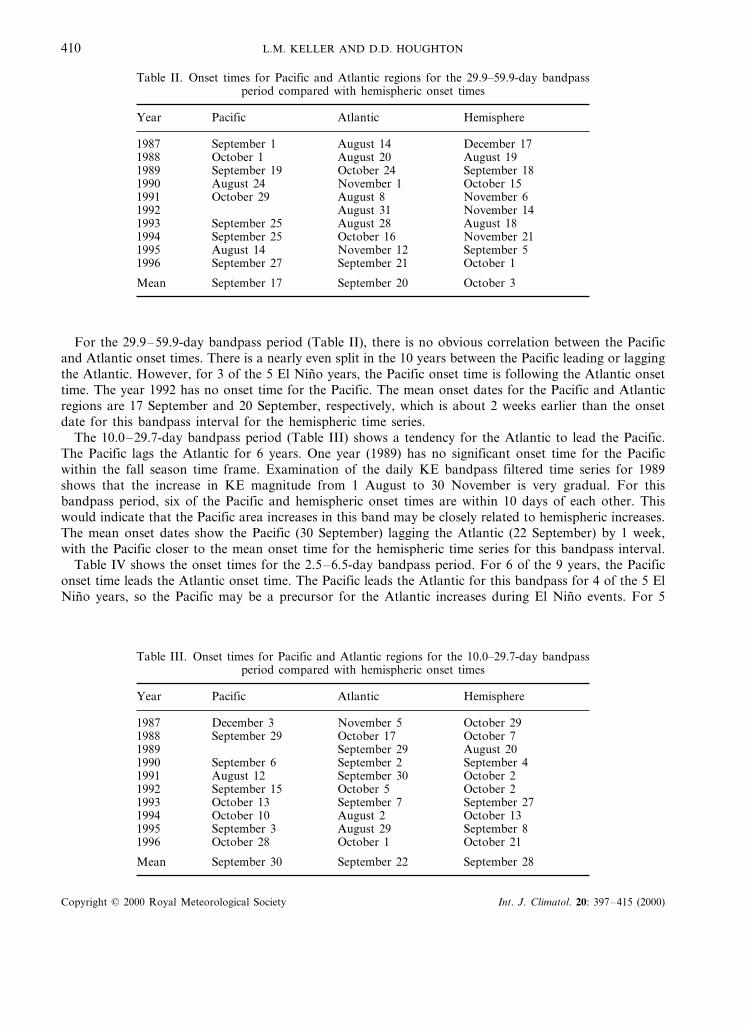
For the 29.9–59.9-day bandpass period (Table II), there is no obvious correlation between the Pacificand Atlantic onset times. There is a nearly even split in the 10 years between the Pacific leading or laggingthe Atlantic. However, for 3 of the 5 El Nino years, the Pacific onset time is following the Atlantic onsettime. The year 1992 has no onset time for the Pacific. The mean onset dates for the Pacific and Atlanticregions are 17 September and 20 September, respectively, which is about 2 weeks earlier than the onsetdate for this bandpass interval for the hemispheric time series.

The 10.0–29.7-day bandpass period (Table III) shows a tendency for the Atlantic to lead the Pacific.The Pacific lags the Atlantic for 6 years. One year (1989) has no significant onset time for the Pacificwithin the fall season time frame. Examination of the daily KE bandpass filtered time series for 1989shows that the increase in KE magnitude from 1 August to 30 November is very gradual. For thisbandpass period, six of the Pacific and hemispheric onset times are within 10 days of each other. Thiswould indicate that the Pacific area increases in this band may be closely related to hemispheric increases.The mean onset dates show the Pacific (30 September) lagging the Atlantic (22 September) by 1 week,with the Pacific closer to the mean onset time for the hemispheric time series for this bandpass interval.

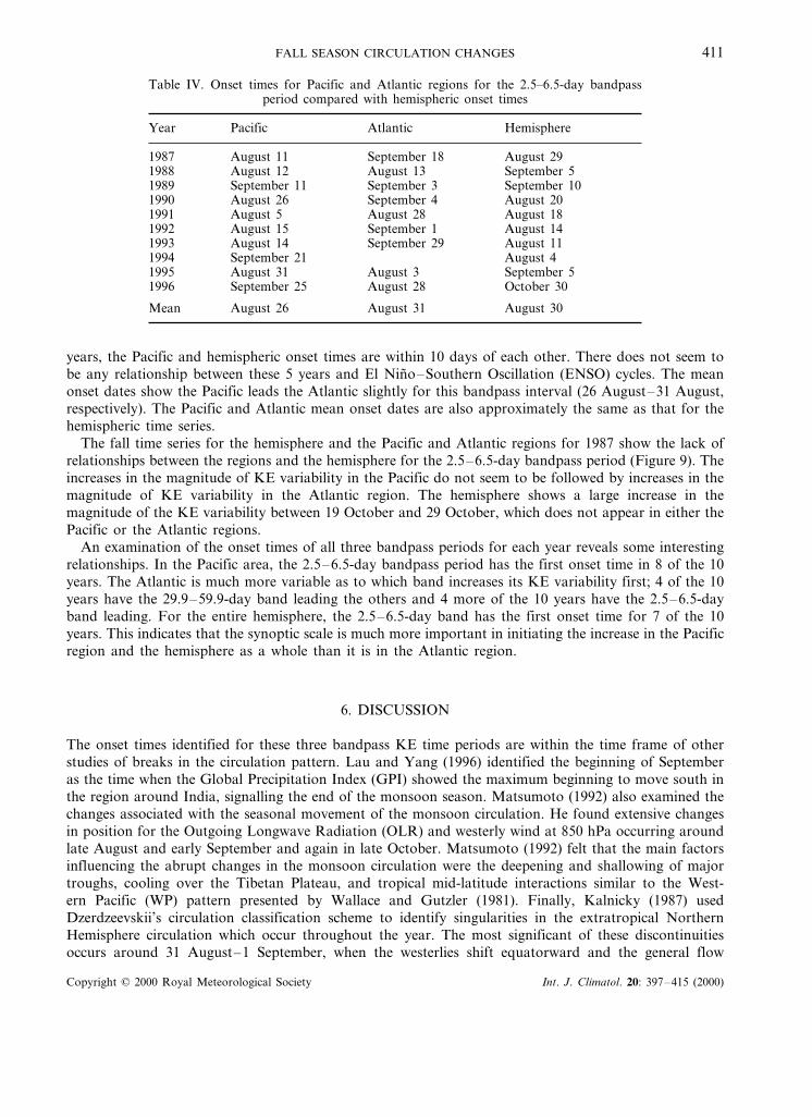
Table IV shows the onset times for the 2.5–6.5-day bandpass period. For 6 of the 9 years, the Pacificonset time leads the Atlantic onset time. The Pacific leads the Atlantic for this bandpass for 4 of the 5 ElNino years, so the Pacific may be a precursor for the Atlantic increases during El Nino events. For 5

Table III. Onset times for Pacific and Atlantic regions for the 10.0–29.7-day bandpassperiod compared with hemispheric onset times

Pacific AtlanticYear Hemisphere

November 5December 3 October 291987September 291988 October 17 October 7

1989 August 20September 29September 2September 61990 September 4

October 2September 301991 August 121992 September 15 October 5 October 2

October 131993 September 7 September 27October 101994 August 2 October 13

September 8August 29September 319951996 October 28 October 1 October 21

September 28September 22September 30Mean



Table IV. Onset times for Pacific and Atlantic regions for the 2.5–6.5-day bandpassperiod compared with hemispheric onset times

Year Pacific Atlantic Hemisphere

1987 August 11 September 18 August 291988 August 12 August 13 September 51989 September 11 September 3 September 101990 August 26 September 4 August 201991 August 5 August 28 August 181992 August 15 September 1 August 141993 August 14 September 29 August 111994 September 21 August 41995 August 31 August 3 September 51996 September 25 August 28 October 30

Mean August 26 August 31 August 30

years, the Pacific and hemispheric onset times are within 10 days of each other. There does not seem tobe any relationship between these 5 years and El Nino–Southern Oscillation (ENSO) cycles. The meanonset dates show the Pacific leads the Atlantic slightly for this bandpass interval (26 August–31 August,respectively). The Pacific and Atlantic mean onset dates are also approximately the same as that for thehemispheric time series.

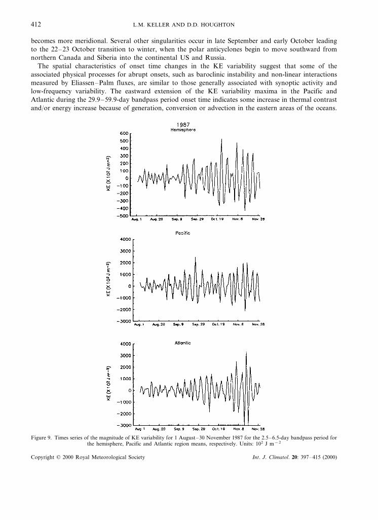
The fall time series for the hemisphere and the Pacific and Atlantic regions for 1987 show the lack ofrelationships between the regions and the hemisphere for the 2.5–6.5-day bandpass period (Figure 9). Theincreases in the magnitude of KE variability in the Pacific do not seem to be followed by increases in themagnitude of KE variability in the Atlantic region. The hemisphere shows a large increase in themagnitude of the KE variability between 19 October and 29 October, which does not appear in either thePacific or the Atlantic regions.

An examination of the onset times of all three bandpass periods for each year reveals some interestingrelationships. In the Pacific area, the 2.5–6.5-day bandpass period has the first onset time in 8 of the 10years. The Atlantic is much more variable as to which band increases its KE variability first; 4 of the 10years have the 29.9–59.9-day band leading the others and 4 more of the 10 years have the 2.5–6.5-dayband leading. For the entire hemisphere, the 2.5–6.5-day band has the first onset time for 7 of the 10years. This indicates that the synoptic scale is much more important in initiating the increase in the Pacificregion and the hemisphere as a whole than it is in the Atlantic region.

6. DISCUSSION

The onset times identified for these three bandpass KE time periods are within the time frame of otherstudies of breaks in the circulation pattern. Lau and Yang (1996) identified the beginning of Septemberas the time when the Global Precipitation Index (GPI) showed the maximum beginning to move south inthe region around India, signalling the end of the monsoon season. Matsumoto (1992) also examined thechanges associated with the seasonal movement of the monsoon circulation. He found extensive changesin position for the Outgoing Longwave Radiation (OLR) and westerly wind at 850 hPa occurring aroundlate August and early September and again in late October. Matsumoto (1992) felt that the main factorsinfluencing the abrupt changes in the monsoon circulation were the deepening and shallowing of majortroughs, cooling over the Tibetan Plateau, and tropical mid-latitude interactions similar to the West-ern Pacific (WP) pattern presented by Wallace and Gutzler (1981). Finally, Kalnicky (1987) usedDzerdzeevskii’s circulation classification scheme to identify singularities in the extratropical NorthernHemisphere circulation which occur throughout the year. The most significant of these discontinuitiesoccurs around 31 August–1 September, when the westerlies shift equatorward and the general flow



becomes more meridional. Several other singularities occur in late September and early October leadingto the 22–23 October transition to winter, when the polar anticyclones begin to move southward fromnorthern Canada and Siberia into the continental US and Russia.

The spatial characteristics of onset time changes in the KE variability suggest that some of theassociated physical processes for abrupt onsets, such as baroclinic instability and non-linear interactionsmeasured by Eliassen–Palm fluxes, are similar to those generally associated with synoptic activity andlow-frequency variability. The eastward extension of the KE variability maxima in the Pacific andAtlantic during the 29.9–59.9-day bandpass period onset time indicates some increase in thermal contrastand/or energy increase because of generation, conversion or advection in the eastern areas of the oceans.

Figure 9. Times series of the magnitude of KE variability for 1 August–30 November 1987 for the 2.5–6.5-day bandpass period forthe hemisphere, Pacific and Atlantic region means, respectively. Units: 102 J m−2



Wintertime observational and modelling studies confirm the enhancement of the variability of thelarge-scale flow related to an increase in the interaction with synoptic scale eddies across the Pacific andAtlantic oceans (Sheng and Derome, 1993; Branstator, 1995; Orlanski, 1998). An increase of eddyavailable potential energy (APE) associated with synoptic scale activity as well as development andmovement of the large-scale flow patterns has also been found in the eastern ocean areas in winter(Koehler and Min, 1984; Lee and Mak, 1995). The eastward shifts in the jet maxima in the Pacific andAtlantic ocean areas would be expected during winter because of the conversion of eddy APE to KE inthese regions.

7. CONCLUSIONS

An analysis of observations for atmospheric circulations in the Northern Hemisphere has identifiedabrupt change characteristics in the seasonal cycle for KE features. Specifically, the time fluctuations ofdomain-averaged vertically-integrated KE were shown to have particular times of significant abruptincreases in amplitudes in the fall transition season. This characteristic was found for both hemispheric-averaged KE and KE averaged over Pacific and Atlantic Ocean area sectors. Significant abrupt increaseswere found for individual bandpass intervals in the time spectrum of variability (with period intervals of29.9–59.9, 10.0–29.7 and 2.5–6.5 days, respectively). The analysis identified at least one significantabrupt increase in variability for hemispheric-averaged KE in each of the 10 years for each of the threefrequency bands identified above. The analysis focused on the time of the first significant abrupt increasein the season in each frequency band, designated as the ‘onset’ time.

The fall season onset times varied greatly from year to year and among the frequency bands. In general,the onset times tended to be earlier for the higher frequency spectral bands. The mean dates for the onsettimes were 30 August, 28 September and 3 October for the 2.5–6.5, 10.0–29.7 and 29.9–59.9-daybandpass periods, respectively. The interannual variability of the onset dates tended to be larger for thelower frequency spectral bands and had ranges of 87, 71 and 122 days for the 2.5–6.5, 10.0–29.7 and29.9–59.9-day bandpass periods, respectively. Without the extremely late onset date in 1996 for the2.5–6.5-day bandpass period, the interannual variability would be 37 days.

Interannual variability of the onset dates may be indicative of overall variability in the seasonal cycle,which has important consequences for interannual variability in other components of the ocean–atmosphere system, such as sea surface temperatures (SSTs). For example, an early fall could have coolerair moving over the Pacific at an earlier time of the year. This could cause enhanced sensible and latentheat fluxes which would act to cool the ocean SSTs more than with a late fall. The cooler SSTs could theninfluence the middle latitude circulation patterns and onset characteristics in the atmosphere during thesubsequent winter and perhaps even into the spring.

Compositing the time series for the hemispheric-average KE for each of the bandpass intervals on eachof the respective onset days provides a robust description of the signal for increase in variability at theonset time. This signal is qualitatively similar for all the bandpass intervals. Compositing is useful only fortimes near the onset time as the non-stationarity of the KE variability in the bandwidth leads tosignificant out-of-phase effects away from the onset time.

Composites of the large-scale horizontal spatial patterns of KE, with respect to the onset times for thehemispheric average, help to suggest physical processes that may be related to the onset event. Thirty-daycomposite means of variability amplitudes for prior to and following the onset time reveal that theprimary centres of activity correspond to the main tropospheric jet stream locations in the western Pacificand Atlantic Ocean areas. The Pacific is clearly the most dominant region. The 29.9–59.9-day bandpassinterval composites show an increase in magnitude of the KE variability and an eastward and westwardextension of this increase in both the Pacific and Atlantic sectors over the onset period. The 10.0–29.7-daybandpass period composites over the onset period display primary increases in the variability magnitudes,with little extension of the area of largest variability. The 2.5–6.5-day bandpass period composites showincreases of KE variability across much of the Pacific area and North America. For the North Atlantic,



the region of smaller increases is positioned just south of Greenland, a favoured area for secondarycyclogenesis.

Analysis of onset characteristics for KE time series means for the Pacific and Atlantic Ocean areasseparately provides further insight into the relationships between the Pacific and Atlantic regions. For the29.9–59.9-day bandpass period, there is little correlation between the Pacific and Atlantic onset times andlittle evidence that the onset time in one region consistently leads that in the other. For the 10.0–29.7-daybandpass period, the Atlantic tends to lead the Pacific area. For the 2.5–6.5-day bandpass interval, thePacific region onset time tends to occur prior to that in the Atlantic area. Thus, the Pacific and Atlanticregions seem to be operating independently in the lower frequency band. Partial decoupling between thePacific Ocean and Atlantic–Eurasian sectors has been alluded to by Kimoto and Ghil (1993) in theiranalysis of flow regimes in the winter season. They concluded that although hemispheric coherent regimesmay or may not be significant, hemispheric regimes arise because of dynamical events that exhibited moresectorially confined features.

Identifying and understanding the physical processes leading to the abrupt onset of the fall transitionseason will be a major challenge for future research. Several physical processes seem to be candidates forhaving a major influence on the abrupt changes in circulation patterns. This paper shows that abruptchanges in monsoon circulation and OLR distribution occur around the time of the identified abruptonset. Tropical influence has been noted by relationships between ENSO cycles and onset date timing.Tziperman et al. (1994, 1997) used model studies to establish the mechanisms by which the seasonality ofthe background state interacts with the interannual variability to develop ENSO events. These events havealready been shown to peak in the fall season (Rasmusson and Carpenter, 1982). Finally, instabilitymechanisms relating to barotropic and baroclinic effects, other baroclinic effects on the synoptic andplanetary circulation, and regime equilibrium instability which causes a hemispheric scale rearrangementof the circulation pattern could all play a role.

The study of physical processes will also require a more complete description of both spring and falltransition season characteristics. Preliminary work indicates that the spring season characteristics aredifferent from those of the fall, so it is quite possible that the important trigger processes may be differentwith the different seasons.

ACKNOWLEDGEMENTS

This study was supported by the National Science Foundation under Grants ATM-9302884 andATM-9711750.

REFERENCES

Borges, M.D. and Hartmann, D.L. 1992. ‘Barotropic instability and optimal perturbations of observed nonzonal flows’, J. Atmos.Sci., 49, 335–354.

Branstator, G. 1995. ‘Organization of storm track anomalies by recurring low-frequency circulation anomalies’, J. Atmos. Sci., 52,207–226.

Dole, R.M. 1989. ‘Life cycles of persistent anomalies. Part I: evolution of 500 mb height anomalies’, Mon. Wea. Re6., 117, 177–211.Dole, R.M. and Black, R.X. 1990. ‘Life cycles of persistent anomalies. Part II: the development of persistent negative height

anomalies over the North Pacific Ocean’, Mon. Wea. Re6., 118, 824–846.Fleming, E.L., Lim, G.H. and Wallace, J.M. 1987. ‘Differences between the spring and autumn circulation in the Northern

Hemisphere’, J. Atmos. Sci., 44, 1266–1286.Ghil, M. 1987. ‘Dynamics, statistics, and predictability of planetary flow regimes’, in Nicolis, C. and Nicolis, G. (eds), Irre6ersible

Phenomena and Dynamical Systems Analysis in Geosciences, Reidel, Dordrecht, pp. 241–283.Goddard, L. and Graham, N.E. 1997. ‘El Nino in the 1990s’, J. Geophys. Res., 102, 10423–10436.Hansen, A.R. and Sutera, A. 1992. ‘Structure in the phase space of a general circulation model deduced from empirical orthogonal

functions’, J. Atmos. Sci., 49, 320–326.Kalnicky, R.A. 1987. ‘Seasons, singularities, and climate changes over the midlatitudes of the Northern Hemisphere during

1899–1969’, J. Clim. Appl. Meteor., 26, 1496–1510.Kimoto, M. and Ghil, M. 1993. ‘Multiple flow regimes in the Northern Hemisphere winter, Part II: sector regimes and preferred

transitions’, J. Atmos. Sci., 50, 2645–2673.Koehler, T.L. and Min, K.D. 1984. ‘Available potential energy and extratropical cyclone activity during the FGGE year’, Tellus,

36A, 64–75.



Lau, K.-M. and Peng, L. 1992. ‘Dynamics of atmospheric teleconnections during the northern summer’, J. Climate, 5, 140–158.Lau, K.-M. and Yang, S. 1996, ‘Seasonal variation, abrupt transition, and intraseasonal variability associated with the Asian

summer monsoon in the GLA GCM’, J. Climate, 9, 965–985.Lee, W.-J. and Mak, M. 1995. ‘Dynamics of storm tracks: a linear instability perspective’, J. Atmos. Sci., 52, 697–723.Lorenz, E.N. 1990. ‘Can chaos and intransitivity lead to interannual variability?’, Tellus, 42A, 378–389.Madden, R.A. and Julian, P. 1971. ‘Detection of a 40–50 day oscillation in the zonal wind in the tropical Pacific’, J. Atmos. Sci.,

28, 702–708.Matsumoto, J. 1992. ‘The seasonal changes in Asian and Australian monsoon regions’, J. Meteorol. Soc. Jpn., 70, 257–273.Mo, K. and Ghil, M. 1988. ‘Cluster analysis of multiple planetary flow regimes’, J. Geophys. Res., 93, 10927–10952.Molteni, F. and Palmer, T.N. 1993. ‘Predictability and finite-time instability of the northern winter circulation’, Q.J.R. Meteorol.

Soc., 119, 269–298.Namias, J. 1952. ‘The annual course of month-to-month persistence in climate anomalies’, Bull. Am. Meteor. Soc., 33, 279–285.Namias, J. 1988. ‘Abrupt change in climate regime from summer to fall 1985 and stability in the fall’, Meteor. Atmos. Phys., 38,

34–41.Namias, J. 1990. ‘Basis for prediction of the sharp reversal of climate from autumn to winter 1988–1989’, Intl. J. Climatol., 10,

659–678.Orlanski, I. 1998. ‘Poleward deflection of storm tracks’, J. Atmos. Sci., 55, 2577–2602.Otto-Bliesner, B.L. 1980. The Dynamics of Seasonal Change of the Long Wa6es as Deduced from a Low-Order General Circulation

Model, PhD Dissertation, University of Wisconsin-Madison. [Available from Dr D.D. Houghton, 1225 W. Dayton St., Madison,WI 53706, USA.]

Press, W.H., Teukolsky, S.A., Vetterling, W.T. and Flannery, B.P. 1992. Numerical Recipes in FORTRAN, Cambridge UniversityPress, Cambridge, pp. 609–613.

Rasmusson, E.M. and Carpenter, T.H. 1982. ‘Variations in tropical sea surface temperature and surface wind fields associated withthe Southern Oscillation/El Nino’, Mon. Wea. Re6., 110, 354–384.

Raymond, W.H. 1988. ‘High-order low-pass implicit tangent filters for use in finite area calculations’, Mon. Wea. Re6., 116,2132–2141.

Reinhold, B. and Yang, S. 1993. ‘The role of transients in weather regimes and transitions’, J. Atmos. Sci., 50, 1173–1180.Sechrist, F.S. and Rudy, R.A. 1969. ‘Kinetic energy changes in a developing cyclone’, Studies of Large Scale Atmospheric Energetics,

Final Report for ESSA Grant WBG 52, pp. 93–114. [Available from L.M. Keller, 1225 W. Dayton St. Madison, WI 53706,USA.]

Sheng, J. and Derome, J. 1993. ‘Dynamic forcing of the slow transients by synoptic-scale eddies: an observational study’, J. Atmos.Sci., 50, 757–771.

Tao, S.-Y. and Chen, L.-X. 1987. ‘A review of recent research on the Asian summer monsoon in China’, in Chang, C.-P. andKrishnamurti, T.N. (eds), Monsoon Meteorology, Oxford University Press, Oxford, pp. 60–92.

Trenberth, K.E. 1992. Global Analyses from ECMWF and Atlas of 1000 to 10 mb Circulation Statistics, NCAR Technical NoteNCAR/TN-373+STR, NCAR, Boulder, CO 80307 USA.

Trenberth, K.E. 1997. ‘The definition of El Nino’, Bull. Am. Meteor. Soc., 78, 2771–2777.Tziperman, E., Stone, L., Cane, M.A. and Jarosh, H. 1994. ‘El Nino chaos: overlapping of resonances between the seasonal cycle

and the Pacific Ocean–atmosphere oscillator’, Science, 264, 72–74.Tziperman, E., Zebiak, S.E. and Cane, M.A. 1997. ‘Mechanisms of seasonal–ENSO interaction’, J. Atmos. Sci., 54, 61–71.Wahl, E. 1972. ‘Climatological studies of the large-scale circulation in the Northern Hemisphere, I. Zonal and meridional indices at

the 700-mb level’, Mon. Wea. Re6., 100, 553–564.Wallace, J.M. and Gutzler, D.S. 1981. ‘Teleconnections in the geopotential height field during the Northern Hemisphere winter’,

Mon. Wea. Re6., 109, 785–812.Wang, B. and Xu, X. 1997. ‘Northern Hemisphere summer monsoon singularities and climatological intraseasonal oscillation’. J.

Climate, 10, 1071–1085.Yeh, T.-C., Dao, S.-Y. and Li, M.-T. 1959. ‘The abrupt changes of circulations over the Northern Hemisphere during June and

October’, in Bolin, B. (ed.), Atmosphere and Sea in Motion, Rossby Memorial Volume, The Rockefeller Institute Press, New York,pp. 249–267.

Zeng, Q.-C., Yuan, C.-G., Zhang, X.-H., Liang, X.-Z. and Bao, B.-N. 1988. ‘A global gridpoint general circulation model’,Collection of Papers presented at the WMO/IUGG NWP Symposium, Tokyo, Japan, 4–8 August 1986, Geneva, pp. 421–430.

Zeng, Q.-C., Zhang, B.-L., Liang, X.-L. and Zhao, S.-X. 1994. ‘East Asian summer monsoon’, in Das, P.K. (ed.), Recent Ad6ancesin Atmospheric Physics, Indian National Science Academy, New Delhi, pp. 81–96.


Documents

Characteristics of the large-scale circulation changes during the sudden onset of the fall transition season