Characterising gadofosveset for use in quantitative … gadofosveset for use in quantitative MRI studies ... Chapters 4, 7); Peter Hine, ... 3.1.3 Pharmacokinetics

I

Characterising gadofosveset for use

in quantitative MRI studies

Owen Carl Richardson

Submitted in accordance with the requirements for the degree of

Doctor of Philosophy (PhD)

The University of Leeds

School of Medicine

September 2013

II

The candidate confirms that the work submitted is his own, except where work

which has formed part of jointly-authored publications has been included. The

contribution of the candidate and the other authors to this work has been

explicitly indicated below. The candidate confirms that appropriate credit has

been given within the thesis where reference has been made to the work of

others.

Chapter 6 is based on the jointly authored publication:

RICHARDSON, O. C., M. L. J. SCOTT, S. F. TANNER, J. C. WATERTON and

D. L. BUCKLEY. 2012. Overcoming the low relaxivity of gadofosveset at high

field with spin locking. Magnetic Resonance in Medicine, 68(4), pp.1234-1238.

All authors contributed to the concept; OCR wrote the majority of the text, with

some contribution from other authors; OCR acquired all data at 0.47 T and was

assisted by MLJS in data acquisition at 4.7 T; OCR carried out all data analysis

and generated plots; all authors contributed to conclusions.

This copy has been supplied on the understanding that it is copyright material

and that no quotation from the thesis may be published without proper

acknowledgement.

© 2013 The University of Leeds and Owen Carl Richardson

III

Acknowledgements

This project was carried out with the aid of a BBSRC industrial CASE award

(BB/G017220/1), in partnership with Astrazeneca. I am grateful to my sponsors

for their financial support. For assistance with data acquisition I would also like

to acknowledge the support of: Neil Woodhouse, José Ulloa, Hervé Barjat, and

co-workers, AstaZeneca (Image acquisition, Chapters 4, 6, 7); Chris Smith,

Steve Hill, AstraZeneca (ICP-MS, Chapter 5); Peter Wright (formerly of

LMBRU), Arshad Zaman, Leeds Teaching Hospitals NHS Trust (Image

acquisition, Chapters 4, 7); Peter Hine, Michael Ries, University of Leeds

Department of Physics (NMR measurements, Chapters 4, 6); Octavia Bane,

Tim Carroll, Michael Markl, Northwestern University, Chicago, imaging

volunteers and staff at Northwestern Memorial Hospital, Chicago (Image

acquisition, Chapter 7); Thomas Oerther, Bruker BioSpin GmbH (Spin-locking

imaging sequence, Chapter 6). For valuable advice, support and suggestions

throughout the project, I would like to thank John Waterton at AstraZeneca. For

first introducing me to the wonderful world of MRI, I am grateful to Sasha

Radjenovic, John Ridgway, Sarah Bacon and Dan Wilson. For being an

inspirational and helpful bunch of people to work with, I’d like to thank the other

members of Medical Physics (and support staff) at Leeds, in particular fellow

book-clubbers John Biglands and Dave Broadbent.

Above all, I extend unreserved thanks to my fantastic supervision team, David

Buckley, Steve Tanner, Marietta Scott and Steven Sourbron. I am particularly

indebted to David, for the dedication he has shown to this project and the

generosity he has displayed in giving his time and lending his experience.

On a personal note I would like to thank my family for their support. In

particular, I would like to thank my partner Sharon for allowing me to turn our

lives upside down (temporarily, I promise!), and for everything else – especially

for our daughter, Isabel. It is to Isabel I would like to dedicate this thesis; I hope

that one day she understands what an inspiration she is to me.

IV

Abstract

Background: Gadofosveset is a clinically approved gadolinium-based MRI

contrast agent that displays altered pharmacokinetic properties due to its high

albumin-binding affinity (around 90% binds at low concentration), although the

improved effectiveness due to binding reduces as field strength increases. With

the trend for increasing clinical magnetic field strengths, it is important that

gadofosveset is fully characterised at higher fields. It may then be possible to

utilise the macromolecular properties of bound gadofosveset in tracer kinetic

modelling for assessment of functional parameters.

Aims: This study aimed to characterise gadofosveset, in vitro, at relevant field

strengths, develop a method for acquiring blood concentration measurements,

and assess several novel techniques utilising the agent’s binding affinity. The

study was extended to include gadoxetate and gadobenate, gadolinium agents

with a lower albumin-binding affinity, to provide a broader view of the influence

of albumin binding.

Results: Relaxivities were calculated from in vitro measurements in the

presence and absence of albumin, including bound relaxivity values at high

field that have not previously been published. Extending the conventional

model assumption of a single binding site to include up to three bound

molecules improved the model fit for gadofosveset at low fields. A technique for

using micro-samples of blood to measure gadolinium levels was successfully

demonstrated in vitro, which may enable improved accuracy in dynamic

studies. A macromolecule-sensitive technique (spin locking) gave a significant

increase in albumin-bound gadofosveset relaxation rates at high field. A

method for using gadofosveset as a biomarker for albumin was successfully

applied in vitro, and the feasibility of in vivo implementation was assessed.

Conclusions: This in vitro characterisation of gadofosveset across a range of

field strengths may inform future in vivo tracer kinetic modelling studies.

Several novel applications for exploiting these characteristics have been

successfully demonstrated in vitro, and warrant further in vivo investigation.

V

Table of Contents

Acknowledgements .................................................................................... III

Abstract ...................................................................................................... IV

Table of Contents ........................................................................................ V

List of Tables ............................................................................................... X

List of Figures ............................................................................................ XI

CHAPTER 1: INTRODUCTION ..................................................................... 1

1.1 BACKGROUND ............................................................................... 1

1.2 AIMS AND OBJECTIVES ................................................................ 2

1.3 OVERVIEW OF CHAPTERS ........................................................... 4

CHAPTER 2: BACKGROUND ...................................................................... 6

2.1 INTRODUCTION TO MRI ................................................................ 6

2.2 BASIC PRINCIPLES OF MRI .......................................................... 7

2.2.1 Spin and magnetic moments................................................. 7

2.2.2 Generating clinical images .................................................. 12

2.2.3 Pulse sequences overview ................................................. 14

2.3 CONTRAST AGENTS ................................................................... 18

2.3.1 Contrast agent definition ..................................................... 19

2.3.2 Uses of contrast agents ...................................................... 20

2.3.3 Mode of operation ............................................................... 21

2.3.4 Contrast agent design ......................................................... 24

2.4 GADOLINIUM-BASED CONTRAST AGENTS ............................... 26

2.4.1 Overview of clinically approved agents ............................... 26

2.4.2 Gadofosveset, gadoxetate and gadobenate ....................... 28

2.4.3 Other albumin-binding gadolinium-based agents ................ 29

2.5 NON-GADOLINIUM-BASED CONTRAST AGENTS ..................... 29

2.6 SUMMARY..................................................................................... 30

CHAPTER 3: EXISTING LITERATURE ON GADOFOSVESET AND OTHER ALBUMIN-BINDING AGENTS ............................................... 31

3.1 CHARACTERISING GADOFOSVESET ........................................ 31

3.1.1 Development of gadofosveset............................................. 31

3.1.2 Binding ................................................................................ 32

3.1.3 Pharmacokinetics ................................................................ 38

VI

3.1.4 Relaxivity ............................................................................ 39

3.1.5 Injection protocol ................................................................. 42

3.1.6 Safety .................................................................................. 42

3.2 CLINICAL APPLICATIONS AND PREVIOUS RESEARCH ........... 43

3.3 OTHER CLINICALLY APPROVED ALBUMIN-BINDING CONTRAST AGENTS, GADOXETATE AND GADOBENATE ..... 45

3.3.1 Background ......................................................................... 45

3.3.2 Clinical applications ............................................................ 48

3.4 NON-CLINICALLY APPROVED ALBUMIN-BINDING AGENTS .... 50

3.5 SUMMARY..................................................................................... 51

CHAPTER 4: EXPLORING THE LONGITUDINAL RELAXIVITY OF GADOFOSVESET AND OTHER ALBUMIN-BINDING AGENTS AT VARIOUS MAGNETIC FIELD STRENGTHS ...................................... 53

4.1 BACKGROUND ............................................................................. 53

4.2 AIMS AND OBJECTIVES .............................................................. 54

4.3 THEORY ........................................................................................ 56

4.3.1 Determining relaxivity .......................................................... 56

4.3.2 Assessing binding sites ....................................................... 57

4.4 METHOD ....................................................................................... 59

4.4.1 In vitro solutions .................................................................. 59

4.4.2 Measurements at 0.47 T ..................................................... 60

4.4.3 Measurements at 3.0 T ....................................................... 60



4.4.6 Calculating relaxation rate, R1 ............................................. 62

4.4.7 Relaxivity ............................................................................ 64

4.4.8 Additional binding sites ....................................................... 64

4.5 RESULTS ...................................................................................... 64

4.6 DISCUSSION ................................................................................. 71

4.6.1 Relaxation rates .................................................................. 71

4.6.2 Relaxivity ............................................................................ 72

4.6.3 Multiple binding sites ........................................................... 73

4.6.4 Species differences: gadofosveset ..................................... 75

4.6.5 Limitations ........................................................................... 75

4.6.6 Summary ............................................................................ 77

VII

CHAPTER 5: A THEORETICAL APPPROACH TO IN VIVO GADOFOSVESET BLOOD CONCENTRATION MEASUREMENT .... 79

5.1 BACKGROUND ............................................................................. 79

5.1.1 Contrast agent blood concentration .................................... 79

5.1.2 Blood sampling ................................................................... 81

5.1.3 Measuring Gd content ......................................................... 83

5.2 AIMS .............................................................................................. 86

5.3 METHOD ....................................................................................... 87

5.3.1 Sample preparation ............................................................. 88

5.3.2 ICP-MS ............................................................................... 89

5.4 RESULTS ...................................................................................... 89

5.5 DISCUSSION ................................................................................. 93

5.5.1 Method validation ................................................................ 93

5.5.2 Proposed in vivo validation methodology ............................ 95

5.5.3 Potential limitations ............................................................. 97

CHAPTER 6: OVERCOMING THE LOW RELAXIVITY OF GADOFOSVESET AT HIGH FIELD WITH SPIN LOCKING ............... 99

6.1 BACKGROUND ............................................................................. 99

6.2 AIMS AND OBJECTIVES ............................................................ 102

6.3 METHOD ..................................................................................... 103

6.3.1 In vitro solutions ................................................................ 103

6.3.2 Data acquisition: R1ρ ......................................................... 104

6.3.3 Data acquisition: R1 and R2 ............................................... 104

6.3.4 Calculating relaxation rates ............................................... 105

6.4 RESULTS .................................................................................... 106

6.5 DISCUSSION ............................................................................... 109

6.5.1 Spin locking....................................................................... 109

6.5.2 Transverse relaxation rates .............................................. 112

6.5.3 Limitations ......................................................................... 112

6.5.4 Summary .......................................................................... 113

CHAPTER 7: A GADOFOSVESET-BASED BIOMARKER OF TISSUE ALBUMIN CONCENTRATION .......................................................... 114

7.1 BACKGROUND ........................................................................... 114

7.2 AIMS AND OBJECTIVES ............................................................ 116

7.3 THEORY ...................................................................................... 117

7.3.1 Bound fraction ................................................................... 117

VIII

7.3.2 Measuring albumin binding fraction .................................. 119

7.3.3 Measuring albumin concentration ..................................... 120

7.3.4 Measuring bound relaxivity ............................................... 121

7.4 EXPERIMENTAL METHOD ......................................................... 122

7.4.1 Simulation ......................................................................... 122

7.4.2 In vitro validation ............................................................... 122

7.4.3 In vitro data acquisition: 3.0 T ........................................... 124

7.4.4 In vitro data acquisition: 4.7 T ........................................... 124

7.4.5 Relaxation rates ................................................................ 125

7.4.6 Calculating relaxivity and Csa ............................................ 125

7.4.7 Temperature adjustment ................................................... 126

7.4.8 In vivo feasibility assessment: 3.0 T .................................. 127

7.5 RESULTS .................................................................................... 129

7.5.1 Simulation ......................................................................... 129

7.5.2 In vitro data at 3.0 T and 4.7 T .......................................... 131

7.6 DISCUSSION ............................................................................... 140

7.6.1 Simulation ......................................................................... 141

7.6.2 In vitro model validation .................................................... 142

7.6.3 In vivo feasibility ................................................................ 146

7.6.4 Summary .......................................................................... 150

CHAPTER 8: SUMMARY AND CONCLUSIONS ...................................... 152

8.1 SUMMARY................................................................................... 152

8.1.1 Experimental results: Relaxivity ........................................ 153

8.1.2 Experimental results: Bound fraction ................................ 154

8.1.3 Experimental results: Binding sites ................................... 155

8.1.4 Experimental results: Gadolinium measurement............... 156

8.1.5 Experimental results: Spin locking .................................... 156

8.1.6 Experimental results: Albumin biomarker .......................... 157

8.2 STUDY LIMITATIONS ................................................................. 157

8.3 AREAS FOR FURTHER INVESTIGATION.................................. 158

8.4 CONCLUSIONS AND FINAL REMARKS .................................... 160

IX

List of References ......................................................................................... i

Bibliography ............................................................................................ xxiii

List of Abbreviations .............................................................................. xxiv

Appendix A: Contrast agent equations ............................................... xxviii

A.1 Inner sphere relaxation .............................................................. xxviii

A.2 Outer sphere relaxation ............................................................... xxx

Appendix B: Supplemental experimental results ................................. xxxi

Appendix C: Derivation of maximum bound fraction ........................ xxxiv

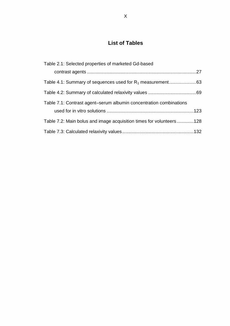
X

List of Tables

Table 2.1: Selected properties of marketed Gd-based

contrast agents .................................................................................... 27

Table 4.1: Summary of sequences used for R1 measurement ..................... 63

Table 4.2: Summary of calculated relaxivity values ..................................... 69

Table 7.1: Contrast agent–serum albumin concentration combinations

used for in vitro solutions ................................................................... 123

Table 7.2: Main bolus and image acquisition times for volunteers ............. 128

Table 7.3: Calculated relaxivity values ....................................................... 132

XI

List of Figures

Figure 2.1: Magnetic moment of a spinning charged particle ......................... 8

Figure 2.2: Magnetic moments in an external magnetic field ......................... 8

Figure 2.3: Magnetisation coordinate system .............................................. 10

Figure 2.4: Effect on magnetisation of an RF pulse ..................................... 11

Figure 2.5: Signal recovery and decay curves ............................................ 14

Figure 2.6: Pulse sequence diagrams .......................................................... 16

Figure 2.7: Plots of signal intensity versus inversion time, recovery time

and echo time ...................................................................................... 18

Figure 2.8: Graphical representation of the influence of a chelated Gd ion

on nearby water molecules. ................................................................. 22

Figure 3.1: Molecular structure of gadofosveset .......................................... 31

Figure 3.2: Structural diagram of human serum albumin molecule .............. 33

Figure 3.3: Plot of variation of R1obs with contrast agent concentration ........ 37

Figure 3.4: Comparison of molecular structures of gadoxetate,

gadobenate and gadofosveset ............................................................. 46

Figure 4.1: Measured relaxation rates (R1) for gadofosveset, gadoxetate

and gadobenate in PBS and BSA at room temperature

(approximately 21 °C) at 0.47 T and 3.0 T (all agents), and at 4.7 T

and 9.4 T (gadofosveset only) ............................................................. 65

Figure 4.2: Measured ΔR1 values for gadofosveset in BSA ......................... 66

Figure 4.3: Measured ΔR1 values for gadoxetate and gadobenate in BSA .. 67

Figure 4.4: Calculated bound and free relaxivity values for all three

agents, split by temperature ................................................................. 68

Figure 4.5: Modelling n = 1 – 3 binding sites at all field strengths at room

temperature ......................................................................................... 70

XII

Figure 4.6: Comparison of R1 values at 37 °C for gadofosveset in BSA

and in mouse plasma at 0.47 T and 4.7 T ............................................ 71

Figure 4.7: Effect of Ka on gadofosveset model fit at 0.47 T at 21 °C and

37 °C .................................................................................................... 76

Figure 5.1: Example of a VIF, showing linear rise to peak and

bi-exponential decay ............................................................................ 80

Figure 5.2: Transferring blood to DBS card ................................................. 82

Figure 5.3: Schematic diagram showing the steps in the process of

ICP-MS ................................................................................................ 84

Figure 5.4: Key components in an inductively-coupled plasma mass

spectrometer ........................................................................................ 85

Figure 5.5: Calibration curves showing Gd counts for a range of

gadofosveset concentrations in mouse plasma, using samples taken

from in vitro solutions ........................................................................... 90


gadofosveset concentrations in PBS, using DBS collection method .... 91


gadofosveset concentrations in mouse blood, using DBS collection

method ................................................................................................. 92

Figure 5.8: Proposed blood sampling times ................................................. 97

Figure 6.1: Effect of spin locking on magnetisation .................................... 100

Figure 6.2: Application of spin-locking pulse .............................................. 101

Figure 6.3: R1 values for gadofosveset in BSA and in PBS at 0.47 T and

4.7 T ................................................................................................... 106

Figure 6.4: R1ρ values for gadofosveset in BSA and in PBS and

gadopentetate in BSA at B0 = 4.7 T, B1L = 90 μT ............................... 107

Figure 6.5: R2 values for gadofosveset in BSA and in PBS at 0.47 T and

4.7 T ................................................................................................... 107

Figure 6.6: R1, R1ρ and R2 for gadofosveset in mouse plasma at

B0 = 4.7 T, B1L = 90 μT....................................................................... 108

XIII

Figure 6.7: Comparison of R1ρ values for gadofosveset in BSA, mouse

plasma and PBS at B0 = 4.7 T, B1L = 90 μT ....................................... 108

Figure 6.8: Plot of calculated R1ρ at three B1L values for gadofosveset in

BSA; sample images at B1L = 90 μT, B1L = 25 μT, and B1L = 5 μT ..... 109

Figure 7.1: Modelled variation of bound concentration and bound fraction

with total gadofosveset concentration ................................................ 119

Figure 7.2: Simulated effect of error in measured relaxation rate

(± 10%) on calculated Csa .................................................................. 130

Figure 7.3: Simulated spread of error in calculated Csa for gadofosveset

when applying a 5% standard deviation on ΔR1,2 variability using a

Gaussian distribution ......................................................................... 131

Figure 7.4: ΔR1 and ΔR2 values at 3.0 T (at room temperature) for

gadofosveset and gadopentetate at Csa = 0.3, 0.45 and 0.7 mM, and

gadoxetate and gadobenate at Csa = 0.45 and 0.7 mM .................... 134

Figure 7.5: ΔR1 and ΔR2 values at 4.7 T (at body temperature) for

gadofosveset and gadopentetate at Csa = 0.3, 0.45 and 0.7 mM, and

gadoxetate and gadobenate at Csa = 0.45 and 0.7 mM .................... 135

Figure 7.6: Variation of observed relaxivity with Csa at 3.0 T

and 4.7 T ............................................................................................ 136

Figure 7.7: Calculated bound fraction ........................................................ 137

Figure 7.8: Spread of calculated Csa values ............................................... 138

Figure 7.9: Example of pre-contrast and post-contrast T1 maps ................ 139

Figure 7.10: Calculated gadofosveset and albumin concentrations in left

ventricle and myocardium in healthy volunteers at 3.0 T ................... 140

Figure B.1: Measured relaxation rates (R1) for gadofosveset, gadoxetate

and gadobenate in PBS and BSA at body temperature

(approximately 37 °C) at 0.47 T and 4.7 T (all agents), and at 9.4 T

(gadofosveset only) ........................................................................... xxxi

Figure B.2: Modelling n = 1 – 3 binding sites at all field strengths at body

temperature ...................................................................................... xxxii

XIV

Figure B.3: Modelling n = 1 – 2 binding sites for gadoxetate and

gadobenate at body temperature and at 0.47 T and 4.7 T ............... xxxiii

1

CHAPTER 1: INTRODUCTION

1.1 BACKGROUND

The field of medical imaging has expanded considerably since Roentgen’s

discovery of X-rays at the end of the nineteenth century, with the introduction of

alternative modalities and the implementation of improved technologies and

methodologies. Yet despite these advances, the latest medical imaging

techniques still present an imperfect view of the inner workings of the human

body. There is a need to strengthen further the diagnostic and therapeutic

potential of medical imaging, and it is this requirement that drives the large

research community engaged in the improvement of these imaging techniques.

Magnetic resonance imaging (MRI) is the imaging modality most recently

adopted into everyday clinical life. Although MRI utilises properties of the

simplest and most abundant atom in the human body, hydrogen, image

generation is underpinned by a sophisticated blend of fundamental physics and

advanced technology. In the 40 years since the feasibility of MRI was first

demonstrated, new applications, techniques and opportunities have been

identified and developed, with the latest peer-reviewed research setting the

agenda for future advances.

One area of MRI research, active since the early 1980s, is the improvement of

tissue contrast through the introduction of exogenous contrast agents. Most

clinical applications of MRI contrast agent utilise the paramagnetic properties of

the gadolinium ion, which must be chelated to a ligand to reduce its toxicity.

Differences in chelate design alter the characteristics of each agent, and lead

to a range of practical applications. Amongst the clinically approved

gadolinium-based contrast agents, gadofosveset demonstrates a unique affinity

for serum albumin which sees it binds reversibly and in high fraction on

injection. The bound gadofosveset molecule acquires certain macromolecular

2

properties which influence the effectiveness and pharmacokinetic behaviour of

the contrast agent. Although gadofosveset is primarily used for imaging the

vessels in MR angiography, its macromolecular properties may also have value

in determining functional parameters such as tissue perfusion and capillary

permeability.

Not all gadofosveset binds to albumin and the effectiveness of the contrast

agent (termed ‘relaxivity’) comprises contributions from both the bound and the

free molecule. Previous studies of gadofosveset have assessed the variation in

relaxivity across a range of magnetic field strengths, but generally do not

extend to the higher fields now in regular clinical use (up to 3.0 T). With the

trend for stronger clinical magnets likely to continue, it is important that

gadofosveset is fully characterised at magnetic field strengths that are, or may

become, clinically relevant. It is only by having a full assessment of the

properties of gadofosveset that further applications, beyond angiography and at

higher field strengths, can be successfully implemented.

1.2 AIMS AND OBJECTIVES

The initial aim of the project was to fully characterise gadofosveset and its in

vivo kinetics prior to application of the tracer in pre-clinical and clinical

quantitative dynamic contrast-enhanced MRI studies. Accurate tracer kinetic

modelling requires representative input parameters, therefore there were two

main objectives: firstly, to assess through in vitro measurement the influence of

binding on the relaxivity of gadofosveset and the variation in this relationship

with field strength; and secondly, to utilise this knowledge in vivo by measuring

a vascular input function for gadofosveset and developing extended tracer

kinetic models to account for the reversible binding of the contrast agent. Pre-

clinical in vivo assessment was to be carried out in a murine model, where high

heart rates and low blood volumes add complexity to the measurement of a

vascular input function.

3

However, gadofosveset was withdrawn from the European market shortly after

this project commenced, and as a result it was not possible to carry out the

planned in vivo experiments. The emphasis of this study was shifted towards

further in vitro gadofosveset characterisation, along with in vitro assessment of

a method developed to measure a vascular input function in small mammals.

Through this characterisation work, several novel opportunities to exploit the

albumin-binding nature of the agent became apparent.

This study has addressed gaps in the current gadofosveset literature and

developed novel methods which may have clinical application. To provide a

broader view of the influence of albumin binding on contrast agent behaviour,

the study was extended to include two other gadolinium-based contrast agents,

gadoxetate and gadobenate. These agents also bind to serum albumin, but

have a much lower affinity than gadofosveset. In vitro experiments were

designed using clinically relevant input parameters, and experimental work was

supported by data simulations to provide a broader assessment of the ability to

apply these methods in vivo.

The specific objectives of the study were as follows:

1. Determine the relaxivities of the bound and free molecules for gadofosveset,

gadoxetate and gadobenate at a range of magnetic field strengths.

2. Extend the relaxation rate model beyond the common assumption of a single

binding site on the albumin molecule, to incorporate up to three bound

molecules, and assess the relative merits of each approach.

3. Develop a method for measuring gadolinium concentrations in micro-

samples of blood, which may be used to generate a vascular input function in

small mammals.

4. Measure the impact on relaxation rates when gadofosveset is used at high

field in conjunction with an imaging technique, spin locking, which is sensitive

to macromolecular content.

4

5. Assess the feasibility of using an albumin-binding contrast agent as a

biomarker for tissue albumin.

1.3 OVERVIEW OF CHAPTERS

Chapter 2 begins with an introduction to the fundamental principles of MRI,

including signal generation and the concept of relaxation. The theory behind

paramagnetic contrast agents is discussed, and a general overview of the

properties of gadolinium-based and other contrast agents is provided.

In Chapter 3 the primary focus is on gadofosveset, with a description of its

albumin-binding properties and the influence of binding on relaxivity. A review

of published literature is presented, within the context of gadofosveset

characterisation and clinical application, to indicate the current level of

knowledge associated with this agent. A similar review is also presented for

gadoxetate and gadobenate, along with a brief overview of non-clinically

approved albumin-binding agents.

Chapter 4 is the first of four experimental chapters, investigating the variation of

gadofosveset, gadoxetate and gadobenate longitudinal relaxivities with field

strength and temperature using in vitro samples. An existing model of

relaxation rate is extended to include up to three binding sites.

In Chapter 5 a novel methodology is established for validating blood

concentration levels of gadofosveset and determining a vascular input function,

using a blood sampling technique that is well suited to small-animal studies.

The feasibility of the technique is established using in vitro samples.

In Chapter 6 the macromolecule-sensitive technique of spin locking is applied

to in vitro samples of gadofosveset to assess the feasibility of enhancing the

relaxivity of gadofosveset at high fields. This novel combination of

gadofosveset with spin locking forms the basis of a published paper (1).

5

Chapter 7, the final experimental chapter, explores through computer

simulation and in vitro measurement the feasibility of a theoretical approach for

using gadofosveset as a biomarker for albumin. The theoretical model is then

applied to human volunteer data, using images acquired through collaboration

with a research team in the USA.

Chapter 8 contains a summary of experimental results, discusses novel

findings and draws final conclusions.

6

CHAPTER 2: BACKGROUND

2.1 INTRODUCTION TO MRI

Magnetic resonance imaging (MRI) generates clinical images of high quality,

providing excellent soft tissue contrast without exposing the patient to ionising

radiation. MRI is routinely used for accurate treatment planning and diagnosis;

the UK National Health Service carries out approximately 1.2 million MRI scans

per year (2).

Although MRI has notable advantages, equipment and scanning costs are

higher and examination times may be longer than for other imaging modalities.

Also, the strong magnetic field utilised in MRI (commonly, 1.5 T or 3.0 T) limits

the interventional procedures that may be carried out during scanning, and

precludes its use in patients with certain types of metal implant or pacemaker.

In addition, the small bore of a conventional clinical scanner may be

challenging for sufferers of claustrophobia.

MRI has limitations in areas such as bone or lung imaging, and image quality is

susceptible to the effects of cardiac and respiratory motion. However, MRI has

become the preferred modality for brain, soft tissue and joint imaging, and an

active international research community is ensuring the clinical utility of MRI

continues to grow.

7

2.2 BASIC PRINCIPLES OF MRI

2.2.1 Spin and magnetic moments

A full mathematical description of the theory behind MRI necessitates the

inclusion of quantum mechanics. However, the fundamental principles of MRI

may be adequately described through classical mechanics without the need to

incorporate quantum theory (3). A classical approach is adopted here, and the

reader is directed to other published texts for a quantum mechanical

description (4, 5).

Although MRI is a relatively recent clinical imaging tool, its principles are built

on the foundation of experimental work published in 1946 by Purcell et al (6)

and Bloch (7) relating to nuclear magnetic resonance (NMR). A fundamental

aspect of this work is that a spinning charged particle, such as the positively

charged proton constituting the hydrogen (1H) nucleus, generates an

electromagnetic field and has a magnetic moment, μ, that is proportional to the

spin angular momentum (with a proportionality constant, γ, known as the

gyromagnetic ratio). This magnetic moment may be described by a vector

pointing along the axis of rotation (Fig. 2.1a). In a sample containing many

particles, the directions of these individual vectors at equilibrium in the absence

of a magnetic field is random and the net magnetic moment is zero (Fig. 2.1b).

8

(a) (b)

Figure 2.1: (a) A spinning charged particle (such as the proton in the 1H nucleus) has a magnetic moment along the axis of rotation; (b) in a sample of many such particles, magnetic moments are randomly orientated and the net magnetic moment is zero

If this sample is placed within an external magnetic field, B0, each magnetic

moment begins to precess around the field, keeping a constant angle between

the spin axis and the field (Fig. 2.2).

Figure 2.2: An external magnetic field, B0, is applied, and individual magnetic moments precess around the axis of B0

The rate at which these spins precess is known as the Larmor frequency, ω0,

and is proportional to the strength of the applied magnetic field, B0. The Larmor

frequency is given by Eq. 2.1.

9

[2.1]

where µ = magnetic dipole moment, h = Planck’s constant (6.63 x 10-34 J s),

γ = gyromagnetic ratio.

The sign of the Larmor frequency indicates the direction of spin precession.

Most nuclei have a positive γ, so the Larmor frequency is negative and

precession is in the clockwise direction (when viewed against the direction of

the magnetic field). The 1H nucleus has a gyromagnetic ratio of 42.6 MHz T-1,

which is larger than almost any other nucleus; it is the primary target for clinical

MRI due to a combination of this high gyromagnetic ratio and its abundance in

the body.

The sum of these individual precessing magnetic moments is still very close to

zero, as the direction of the vector is not changed by the magnetic field.

However, small, rapidly fluctuating magnetic fields are generated on a

microscopic scale by electrons and nuclei, and thermally generated interactions

with these microscopic fields eventually leads to a breakdown in the isotropic

nature of the individual magnetic moments. This leads to a slight tendency for

the net magnetic moment to point in the direction of the applied magnetic field,

as this is a lower energy state.

The build-up of magnetisation towards its equilibrium value of M0 in the

direction of the applied B0 field is defined by an exponential time constant, T1,

known as the spin–lattice or longitudinal relaxation time constant. Although the

term ‘lattice’ has its origins in early NMR experiments with the crystal lattice,

the name is still employed when measuring liquids and gases. If the applied

magnetic field were to be switched off, the individual magnetic moments would

eventually revert to their isotropic nature and the longitudinal spin

magnetisation would decay to a value approaching zero. In a three-dimensional

plot, with orthogonal axes in the x, y and z direction, B0 and M0 conventionally

10

point in the z direction (Fig. 2.3a). The magnetisation Mz at time, t, after the B0

field is switched on is given by Eq. 2.2 and plotted in Fig. 2.3b.

( ) (

) [2.2]

(a) (b)

Figure 2.3: When B0 is applied, magnetisation in the z direction (Mz) grows towards an equilibrium value, M0; (a) relative axes; (b) increase in Mz with time, according to Eq. 2.2

This magnetisation in the z direction is generally too small to be measured.

With the magnetic moments precessing around the B0 field (z axis) and the net

magnetic moment pointing in this direction, there is no net magnetisation

perpendicular to the field. However, if every single spin is rotated by 90° around

the x axis by an additional radiofrequency (RF) pulse, the net magnetic moment

will then point along the –y axis, perpendicular to B0 (Fig. 2.4a). The RF pulse

that flips the net magnetisation into the x–y plane is known as the B1 field, and

will only have an effect when operating at the resonant (Larmor) frequency of

the precessing magnetic moments. For the 1H nucleus at a B0 value of 1.5 T

(the most common field strength employed in clinical MRI) the Larmor

frequency is 63.9 MHz.

M0

11

(a) (b) (c)

Figure 2.4: (a) An RF pulse rotates the magnetisation around the x axis into the –y direction; (b) the net magnetic moment still precesses around the z axis in the x–y plane; (c) the decay of magnetisation in the x–y plane and recovery in the z direction follows a spiral path

This transverse magnetic moment still precesses around the z axis, at the

precession frequency of the individual spins (the Larmor frequency) (Fig. 2.4b).

In addition, the transverse component precesses around the axis of the B1 field

at a frequency (γB1) which is much lower than the precession around the B0

axis. The combination of both precessional motions would appear to an outside

observer as a spiralling down from the longitudinal to the transverse plane.

However, when the B1 field is switched off, the transverse magnetisation

decays due to fluctuations in the local magnetic field resulting from random

interactions with neighbouring spins, random motion through regions of

differing magnetic field strength and variations in tissue magnetic susceptibility.

The time constant of this decay, T2, is known as the spin–spin or transverse

relaxation time constant, and is given (within the x–y plane) by Eq. 2.3.

( )

[2.3]

The decay of magnetisation in the x–y plane occurs at the same time as the

recovery of magnetisation in the z axis, and as a result the vector

magnetisation describes a spiral from the x–y plane up to the z axis (Fig. 2.4c).

The rates of change of magnetisation with time in the x, y and z directions, Mx,

My and Mz, respectively, are described by the Bloch equations (7) (Eq. 2.4a –

2.4c).

12

[2.4a]

[2.4b]

( )

[2.4c]

Any intrinsic inhomogeneity in the main magnetic field will contribute to faster

signal loss, acting to shorten T2. The relaxation measure T2* is equivalent to T2

plus the influence of magnetic field inhomogeneity. Both longitudinal and

transverse relaxation occur at the same time, but transverse relaxation is

generally quicker (T2* ≤ T2 ≤ T1). A further measure of relaxation, the spin-lock

relaxation time, T1ρ, requires an additional locking pulse and will be discussed

in Chapter 6. The angle to which the magnetic moment is rotated (90° in the

above example) relates to a specific RF pulse amplitude and direction; by

varying the properties of this pulse, any angle can be selected. The choice of

angle will be discussed further in Section 2.2.3.

The transverse magnetisation generates an oscillating magnetic field

perpendicular to the main magnetic field, which may be detected through the

electrical current induced in a coil detector. As Mz recovers and transverse

magnetisation reduces, the generated signal follows a pattern of free induction

decay. It is this detected signal that is used to create images in MRI.

2.2.2 Generating clinical images

The feasibility of generating images using NMR was first demonstrated in

1973 (8), with improved techniques for reduced scan times and clearer images

developed over subsequent years (9).

13

The subject is placed within a strong magnetic field (commonly, a B0 value of

1.5 T or 3.0 T is used clinically, with higher B0 values used pre-clinically). By

creating a linear magnetic field gradient in the B0 field, the Larmor frequency

varies linearly along the axis of this gradient (according to Eq. 2.1), enabling

slices to be selectively excited through the choice of B1 pulse properties.

Additional gradients in orthogonal directions enable signal detection to be

pinpointed to a specific location within the patient; repeated measurement with

varying gradient parameters enables the generation of spatially encoded

datasets in two or three dimensions. For detailed background information on

the theory behind spatial encoding with gradients and the mathematical

processes involved in converting detected signals to images, the reader is

directed to other published texts (10, 11).

The relaxation time associated with an individual voxel (the smallest unit of

three-dimensional space within a computer image) of tissue is influenced by,

and reflective of, the properties of the tissue within and around that voxel. For

example, the compact structure of solids leads to interactions between

neighbouring nuclei that are constant with time, resulting in a stronger

dephasing effect (and a shorter T2) than in fluids, where nuclei are constantly

experiencing new neighbours. The natural motional frequency of fat is close to

the Larmor frequencies used in MRI; as a result, fat is the tissue type with the

shortest T1 value, with solid tissue having an intermediate T1 and water having

a long T1. As MRI targets the 1H nucleus, proton density also plays a role, with

the highest proton density signal coming from relatively free water molecules,

such as those found in cerebrospinal fluid. Those tissues with relatively little

water content, such as bone or air within the lungs, provide little or no signal.

Example relaxation curves are shown in Fig. 2.5 (based on the magnetisation

recovery and decay equations, Eq. 2.2 and 2.3) for a range of arbitrary T1 and

T2 relaxation times. Note that at time t = T1, 63% of the signal is recovered, with

almost the whole signal recovered at five times T1 (Fig. 2.5a). At t = T2, the

signal has decayed to 37% of the original value (Fig. 2.5b).

14

Figure 2.5: (a) Signal recovery curves for three T1 relaxation times; (b) Signal decay curves for three T2 relaxation times

2.2.3 Pulse sequences overview

At a basic level, the pulse sequences used for image generation require a

combination of RF excitation pulses and spatial encoding gradients, along with

read-out echo detection. The strength of the excitation pulse (frequency,

amplitude and duration), the repetition time (TR, time between excitation

pulses) and the echo time (TE, time between excitation pulse and read-out)

may be altered to generate T1- or T2-weighted images, according to the tissue

of interest. Generally, if a short TR is chosen the variation in signal between

tissue types results primarily from differences in T1, whereas if a long TE is

chosen the variation in signal results from differences in T2.

The two main pulse sequences used are known as spin echo (SE) and gradient

echo (GE), although a range of variants have also been developed (12). The

standard SE sequence uses a 90° excitation pulse followed at time TE/2 by a

180° refocusing pulse and read-out at time TE (Fig. 2.6a), with free induction

decay of the signal occurring between excitation and read-out. The sequence is

repeated after time TR, with variations in spatial encoding for each repetition, in

order to generate sufficient information for a two- or three-dimensional image.

The advantage of the 180° refocusing pulse in the SE sequence is that it

eliminates any dephasing caused by magnetic field inhomogeneity. A multi-

15

echo variation on the SE sequence has a single 90° excitation pulse, followed

by multiple 180° refocusing pulses (each producing a read-out echo at a

different TE) within a single TR. A third variation, fast spin echo, is similar to the

multi-echo approach, in that it employs a single 90° excitation pulse and

multiple 180° refocusing pulses, but this time each echo is also phase encoded

(and the phase encoding reset after each signal measurement) (Fig. 2.6b). The

fast spin echo approach enables images to be acquired more rapidly, and is

also known as turbo spin echo or rapid acquisition with relaxation

enhancement (RARE).

GE sequences generally use an excitation angle of less than 90°, then

generate an echo with a pair of bipolar gradient pulses and repeat the cycle

after a short TR (Fig. 2.6c). There is no 180° pulse to refocus the proton spins,

resulting in a greater sensitivity to magnetic susceptibility effects, with the rate

of decay given by T2*. Between cycles, any residual steady-state transverse

magnetisation may be eliminated by applying spoiling RF pulses or gradients.

Acquisition using GE is quicker than conventional SE as TR is generally

shorter, but signal-to-noise ratios are often lower than for SE sequences and

GE is more prone to susceptibility artefacts.

16

Figure 2.6: (a) Spin echo and (b) fast spin echo (RARE) sequence; horizontal lines in (b) correspond with labels in (a); (c) gradient echo

Many of the pulse sequences applied in the clinic have been adapted for speed

of acquisition. Although this may come at the expense of a perceived loss in

image quality (for example, through reduced spatial resolution), faster

acquisition times have the advantages of reducing image artefacts caused by

movement and enabling improved temporal resolution on dynamic acquisitions.

In addition, faster acquisition times reduce the time spent by the patient on the

MRI scanner, minimising patient discomfort and increasing patient throughput.

Although pulse sequences with longer acquisition times may be impractical for

clinical purposes, these time constraints are lifted for research involving in vitro

solutions and results acquired over longer time periods may give improved

accuracy in relaxation time measurement.

17

Inversion recovery sequences give heavy T1 weighting. Here, a 180° pulse

inverts the magnetisation along the –z axis, and is followed by a 90° pulse to

bring the residual magnetisation into the x–y plane where it may be detected.

The time between the 180° pulse and the 90° pulse is known as the inversion

time (TI). Repeated inversion recovery signal measurements at a range of TIs

enable T1 to be calculated, using Eq. 2.5 (curve shape shown in Fig. 2.7a).

[2.5]

where SI is the measured signal intensity and S0 is the signal intensity at time

t = 0. The modulus is taken because images are usually magnitude

reconstructions (without negative signal intensity values).

Saturation recovery sequences are able to measure T1 more rapidly than using

inversion recovery. Here, multiple 90° RF pulses are applied at a range of TR

values; the first 90° RF pulse is dephased by a spoiling gradient and

subsequent magnetisation developing along the z axis is rotated into the x–y

plane by another 90° pulse and a gradient echo immediately acquired. Signal

intensity is related to T1 according to Eq. 2.6, and the expected curve shape is

shown in Fig. 2.7b.

( ) [2.6]

T2 values may be determined by varying the echo time and fitting signal

intensity measurements using Eq. 2.7 (curve shape shown in Fig. 2.7c).

[2.7]

18

Figure 2.7: Plot of signal intensity versus (a) inversion time (Eq. 2.5), (b) recovery time (Eq. 2.6) and (c) echo time (Eq. 2.7); (a) and (b) represent T1 recovery curves, and (c) represents T2 decay

2.3 CONTRAST AGENTS

In MRI, endogenous contrast between tissue types, resulting from differences

in longitudinal and transverse relaxation times and proton density, may be

selectively emphasised through the variation of pulse sequence parameters.

However, the effectiveness of such tissue contrast is limited in scenarios where

neighbouring tissue types have similar relaxation times or where pathology,

such as a tumour, has comparable relaxation characteristics to its background.

Several techniques have been developed to generate variations in contrast by

manipulation of pulse sequences. Magnetisation transfer uses off-resonance

19

saturation pulses to suppress the signal from protein-bound water molecules,

which gives a technique sensitive to macromolecular content (13). A similar

concept, known as chemical exchange saturation transfer (CEST), utilises a

selective pre-saturation pulse to differentiate bulk water from water bound to an

exogenous contrast agent (14). Spin locking is another technique that is

sensitive to the presence of macromolecules, using an additional locking pulse

to generate relaxation at the (lower) field strength of this pulse rather than the

strength of the main magnetic field (15).

Blood oxygenation levels may be utilised to generate endogenous contrast, by

assessing differences between signal intensities of diamagnetic

oxyhaemoglobin and paramagnetic deoxyhaemoglobin. This technique, known

as blood oxygenation level dependent (BOLD) contrast, is primarily used for

functional brain imaging (16). A similar technique, arterial spin labelling (ASL),

measures perfusion by magnetically ‘tagging’ blood before it flows into the

region of interest (17).

2.3.1 Contrast agent definition

Contrast may also be enhanced through the administration of an exogenous

contrast agent. The term ‘contrast agent’ in the context of this research refers

to a substance that may be administered to a patient with the purpose of

adding value to a medical image. Contrast agents are used in all imaging

modalities, although the mode of operation for MRI agents differs to that of

agents used in other modalities.

An MRI contrast agent has magnetic properties which reduce longitudinal and

transverse relaxation times; its influence is observed through an alteration of

signal intensity in the vicinity of the agent. An agent that reduces longitudinal

relaxation time produces an area of enhanced signal intensity in T1-weighted

images, and may be defined as a positive contrast agent. An agent that

reduces transverse relaxation time gives an area of signal loss on T2-weighted

images, and is often described as a negative contrast agent. In reality, contrast

20

agents reduce both longitudinal and transverse relaxation times, but the extent

to which each is affected varies according to the properties of the agent.

2.3.2 Uses of contrast agents

MRI contrast agents have a range of clinical applications, enabling improved

assessment of damage, disease and response to treatment. Extending this

range of applications, either through the introduction of new contrast agents

with novel properties or by finding novel uses for existing contrast agents,

represents an important area of ongoing research.

Contrast agents induce changes in image signal intensity that may be used to

map the flow of blood, highlighting blood vessels in contrast-enhanced MR

angiography (18) or disruption to the blood–brain barrier in brain imaging (19).

The spatial distribution of a contrast agent may have clinical value; for example,

regions of signal alteration due to contrast agent accumulation (enhancing

fraction) may correlate with regions of tumour growth and may be used as a

prognostic biomarker in carcinoma (20).

The rate of excretion of the agent may aid assessment of kidney (21) or liver

(22) function. Plotting the variation of signal intensity with time provides

parameters related to tissue properties, including onset time, mean gradient,

maximum signal intensity and wash-out characteristics (23). The shape of such

a curve may correlate with tumour malignancy (24), and the area under the

curve is related to blood volume and capillary permeability (25), although

separation of tissue perfusion and capillary permeability characteristics requires

mathematical modelling to account for tracer kinetic behaviour (26). These

parameters may be of particular value when assessing tumour physiology (27)

or regions of necrosis in myocardial infarction (28), for example. Assessment of

microvascular permeability using MRI contrast agents is sensitive to the size of

the agent molecule (29, 30), with macromolecular agents potentially being

more suitable for selective imaging than small-molecule Gd agents (31).

21

2.3.3 Mode of operation

MRI contrast agents have magnetic susceptibility properties which alter intrinsic

tissue relaxation times by modifying the magnetic field in their immediate

vicinity. Unlike other imaging modalities, it is not the contrast agent itself that is

observed; instead, MRI detects the influence of the contrast agent on nearby

water molecules. Paramagnetic MRI contrast agents have a small, positive

susceptibility to magnetic fields, but do not retain their magnetic properties

outside the magnetic field. Superparamagnetic contrast agents have higher

magnetic susceptibility values, and thus have greater influence over the local

magnetic field.

When discussing contrast agents, it is common to use relaxation rates rather

than relaxation times (where the relaxation rate is the inverse of the relaxation

time). For a dilute paramagnetic solution, the observed solvent relaxation rate

(Riobs, 1/Tiobs) is the sum of the relaxation rate of the solvent nuclei in the

absence of the paramagnetic solute (Ri0, 1/Ti0) and the relaxation rate of the

paramagnetic substance (Ri, 1/Ti) at a given concentration (Eq. 2.8) (32).

[2.8]

where i = 1,2.

The relaxation rate of a paramagnetic contrast agent is conventionally linearly

related to its concentration (Cg), such that Eq. 2.8 can be rewritten as Eq. 2.9.

[2.9]

where i = 1,2.

The relaxation rate (Ri) of a paramagnetic contrast agent consists of two

components: inner sphere (IS) and outer sphere (OS) (Eq. 2.10).

22

[2.10]

where i = 1,2.

Inner sphere effects result from one or more water molecules binding in the

inner coordination sphere of the paramagnetic ion and exchanging rapidly with

bulk water molecules. Secondary and outer sphere effects result from water

molecules diffusing through the outer-sphere environment. These effects, and

the correlation times associated with each, are illustrated graphically in Fig. 2.8.

Figure 2.8: Graphical representation of the influence of a chelated Gd ion on nearby water molecules. Inner sphere relaxation is influenced by the correlation time of the coordinated water molecule (τM) and the rotational correlation time (τR); outer sphere relaxation is influenced by the diffusional correlation time (τD)

Inner sphere relaxation

Inner sphere relaxation occurs when a water molecule is associated with the

contrast agent for a sufficient amount of time to form an identifiable chemical

complex (33). The relaxation rate (RiIS) is influenced by the relaxation rate of

the bound water molecule (Rim) and the number of water molecules binding in

the inner coordination sphere, also known as the hydration number; for most

Gd-based agents only one water molecule binds. RiIS is also influenced by the

time spent by the water molecule in the inner sphere (τM), dictated by the

solvent exchange rate (1/τM) (Eq. A.1 – A.2 in Appendix A). An increase in this

correlation time (i.e. a decrease in the exchange rate of the coordinated water

molecule) leads to a reduction in the inner sphere relaxation rate. When this

23

water molecule exchanges very rapidly (i.e. τM << T1m), the relaxation

enhancement experienced by the bulk water is dependent on the relaxation

rate of this coordinated molecule (R1m). An additional factor which has a small

influence on R2IS is the chemical shift difference between the bound water and

the bulk water (resulting from differences in resonant frequencies).

Bound water relaxation rates consist of components representing dipole–dipole

(DD) and scalar (SC, also known as contact) mechanisms of relaxation

(Eq. 2.11).

[2.11]

where i = 1,2.

These components may be calculated using the Solomon–Bloembergen–

Morgan equations (34) (Eq. A.3 – A.6 in Appendix A). Scalar relaxation rates

are influenced by the scalar coupling constant between the electron at the

paramagnetic centre and the proton of the coordinated water molecule, as well

as the electron Larmor frequency and the scalar correlation time (τei). Dipole–

dipole relaxation rates are strongly influenced by the electron spin–proton spin

distance, r (to the inverse sixth power), as well as the nuclear and electron

Larmor frequencies, and dipole–dipole correlation times (τci). These correlation

times may be defined according to Eq. 2.12 and 2.13.

[2.12]

[2.13]

where i = 1,2, τR is the rotational correlation time of the metal–proton vector,

R1e and R2e are the longitudinal and transverse electron spin relaxation rates of

the metal ion.

24

Rie varies with magnetic field and is usually interpreted in terms of a zero-field-

splitting interaction (a quantum effect associated with spin energy states) (35)

(Eq. A.7 – A.9 in Appendix A).

Outer sphere relaxation

As second sphere relaxivity is generally not well characterised (36), the

separate contributions of the second and outer sphere are usually combined

into a single relaxation rate, RiOS (34). This relaxation rate is influenced by the

distance of closest approach of the water molecule and the complex, as well as

the diffusion constants of the water and the complex (Eq. A.10 – A.14 in

Appendix A).

2.3.4 Contrast agent design

The degree to which a contrast agent influences relaxation time is termed

‘relaxivity’; this parameter is generally normalised to contrast agent

concentration and expressed in units of L mmol-1 s-1 (or mM-1 s-1). It is clear

from contrast agent theory that the effectiveness of a contrast agent is

governed by a range of physical and chemical molecular properties. In addition,

relaxivity is affected by experimental and environmental factors including

temperature, pH and B0 field. For small, low-molecular-weight paramagnetic

contrast agents around 60% of the longitudinal and transverse relaxation

results from inner-sphere effects, with the remainder due to outer sphere

interaction and bulk water transfer (33). Superparamagnetic agents have no

inner coordinating molecule and derive all their relaxivity from outer sphere

effects (35).

A linear relationship between contrast agent concentration (Cg) and change in

R1 (ΔR1) or R2 (ΔR2) is often assumed. In this case, for a plot of Cg versus ΔR1

the slope of a line through measured points and the origin represents

25

longitudinal relaxivity (r1); the slope of an equivalent line on a plot of Cg versus

ΔR2 represents transverse relaxivity (r2) (Eq. 2.14).

[2.14]

where i = 1,2.

However, for contrast agents that bind to albumin, a nonlinear relaxation rate

response to contrast agent concentration will be generated due to the variation

of relaxivity with binding fraction (37).

The variation in signal intensity with time (inversion time, repetition time or echo

time) was shown in Fig. 2.7. A change in relaxation rate, induced by the

introduction of a contrast agent, changes the shape of these curves. At low

contrast agent concentration and at a given time point, a linear correlation

between change in signal intensity and contrast agent concentration is often

assumed. However, this assumption of signal linearity is not strictly correct and

may lead to miscalculated pharmacokinetic parameters (38). Signal intensity

enhancement nonlinearity is increased at high contrast agent concentrations

and where T2 shortening effects are neglected (39). Water exchange rates

between cellular and interstitial spaces (40) and solution microviscosity (41)

may also contribute to nonlinearity.

Contrast agents are conventionally categorised according to their magnetic

susceptibility (paramagnetic or superparamagnetic), biodistribution

(extravascular, intravascular, or tissue-specific) and image enhancement

properties (positive or negative). Early work (42) showed the promise of

utilising paramagnetic contrast agents such as orally administered ferric

chloride and inhaled 100% oxygen to enhance natural tissue contrast. Other

paramagnetic metal ion chelates, including gadolinium (Gd), were also being

considered in the early 1980s (43).

Although much research has been carried out using other agents, most

contrast agents currently marketed for clinical use are Gd-based.

26

2.4 GADOLINIUM-BASED CONTRAST AGENTS

Gadolinium is a lanthanide element with an atomic number of 64 and an atomic

mass of 158 in its most common isotope. In its ionic form (Gd3+) it has seven

unpaired electrons in its outer shell, making it ideal for use as a contrast agent.

However, due to similarities in size Gd can block voltage-gated calcium (Ca2+)

channels at very low concentrations, inhibiting processes that require an influx

of Ca2+ and limiting the activity of certain enzymes (44). To reduce its potential

toxicity, Gd may be chelated to a ligand. Early studies of potential Gd chelates

(45) suggested the use of ethylenediaminetetraacetic acid (EDTA) or

diethylenetriaminepentaacetic acid (DTPA). Relaxation time was significantly

reduced with both chelates, but dose experiments with rats found much higher

tolerance for DTPA than EDTA. Gd-DTPA (gadopentetate dimeglumine) now

forms the basis of several of the most commonly used, clinically approved MRI

contrast agents.

2.4.1 Overview of clinically approved agents

Properties of clinically approved agents

All MRI-approved Gd chelates are nine-coordinate complexes, with a ligand

occupying eight of the available binding sites at the metal centre and the ninth

site occupied by a coordinated water molecule (34). Gd contrast agents may be

grouped according to their ligand properties, being either linear or macrocyclic

in structure and ionic or non-ionic in charge. Several agents selectively bind to

albumin, or may target specific organs. The relaxivity of the agent, its safety

profile, pharmacokinetics and excretion pathway are all influenced by the

ligand. A summary of clinically approved Gd-based agents is given in

Table 2.1.

27

Table 2.1: Selected properties of marketed Gd-based contrast agents

* Relaxivity values measured in plasma at 1.5 T and 37 °C (46)

Safety

The chelated Gd molecule is designed to be well tolerated during its journey

through the body. Minor adverse effects, including nausea and hives, occur in a

low number of cases following contrast agent administration, at a similar rate

for all agents (47). Severe anaphylactoid reactions are rare, with an estimated

incidence of 1:100,000 to 1:500,000 (48). In patients with poor renal function,

the clearance rate of the contrast agent is compromised and the chelated

molecule may degrade into a more toxic form, potentially resulting in increased

Gd bone deposition.

The development of nephrogenic systemic fibrosis (NSF), a hardening of

fibrotic tissue found in patients with renal failure, was first linked to

r1 r2

Gadopentetate

dimeglumine

Gd-DTPA

MagnevistLinear Yes 0.1 Renal 4.1 4.6

Gadobenate

dimeglumine

Gd-BOPTA

MultiHanceLinear Yes 0.1

96% renal

4% hepatic6.3 8.7

Gadoxetic acid

disodium salt

Gd-EOB-DTPA

Primovist/EovistLinear Yes 0.025

50% renal

50% hepatic6.9 8.7

Gadofosveset

trisodium

MS-325

Vasovist/AblavarLinear Yes 0.03

95% renal

5% hepatic27.7 72.6

GadodiamideGd-DTPA-BMA

OmniscanLinear No 0.1 Renal 4.3 5.2

GadoversetamideGd-DTPA-BMEA

OptiMARKLinear No 0.1 Renal 4.7 5.2

Gadoterate

meglumine

Gd-DOTA

DotaremMacrocyclic Yes 0.1 Renal 3.6 4.3

GadoteridolGd-HP-DO3A

ProHanceMacrocyclic No 0.1 Renal 4.1 5.0

GadobutrolGd-BT-DO3A

Gadovist/GadavistMacrocyclic No 0.1 Renal 5.2 6.1

Excretion

pathway

Relaxivity *

(mM-1

s-1

)Generic nameAcronym &

Trade nameStructure Ionic?

Standard

clinical dose

(mmol kg-1

)

28

administration of Gd contrast agents by Grobner (49). This link was

strengthened with detection of Gd in the skin of patients with NSF having been

exposed to a Gd-based contrast agent (50). Although the pathophysiology of

NSF is still not fully known, the link to Gd has led to classification of all agents

into high-, intermediate- and low-risk groups, with associated restrictions on

their use (51). Unconfounded cases of NSF have so far been associated with

just three of the Gd agents: gadodiamide, gadoversetamide and gadopentetate,

with gadodiamide accounting for by far the greater majority (51).

2.4.2 Gadofosveset, gadoxetate and gadobenate

Gadofosveset trisodium (gadofosveset) is unique amongst the clinically

approved agents in that it is the only agent which binds in high fraction to

albumin. Through binding, gadofosveset acquires two fundamental properties

associated with macromolecules: its speed of rotation and its extravasation rate

are both reduced. The latter property influences the kinetic behaviour and

excretion rate of the agent, ensuring the bound molecule remains mostly

intravascular and prolonging the time window for imaging at steady state; the

former property has a significant positive effect on its relaxivity, particularly at

lower magnetic field strengths. The intravascular nature of bound gadofosveset

leads to its indicated use in angiography. However, in a scenario of increased

capillary permeability, such as angiogenesis, it is suggested that pathology may

correlate with higher leakage rates and elevated levels of bound gadofosveset

in the extravascular space.

Gadoxetic acid (gadoxetate) and gadobenate dimeglumine (gadobenate) also

bind reversibly to albumin, at a much lower fraction than gadofosveset.

Although both agents demonstrate an increased relaxivity attributable to

albumin binding, the lower binding affinity of these agents limits the extent to

which their behaviour is modified in vivo.

The properties of gadofosveset, gadoxetate and gadobenate will be discussed

in more detail in Chapter 3, along with an in-depth review of current

research literature.

29

2.4.3 Other albumin-binding gadolinium-based agents

Gd permanently bound to albumin (albumin-Gd-DTPA) has been used as a

macromolecular agent in animal studies (for example,(39, 52)), although the

excessive retention time of this agent makes it less suitable for human studies.

Other attempts to create a macromolecular Gd-based agent include the

conjugation of Gd chelates to synthetic polymers (53) or to a polyethylene

glycol core (54). Biodegradable polydisulfide Gd complexes (55) may prove to

be a safer alternative to some macromolecular agents. In addition to these

synthetic macromolecular agents, a range of Gd-based contrast agents are

being developed to target specific organs or respond to changes in pH,

temperature or enzyme activity (56).

2.5 NON-GADOLINIUM-BASED CONTRAST AGENTS

Although the main focus of this research is on the Gd-based contrast agent

gadofosveset, with a broader assessment of the other clinically approved

albumin-binding agents gadoxetate and gadobenate, it should be noted that a

range of alternative MRI contrast enhancement options are available. Other

lanthanide ions such as dysprosium (Dy3+) and holmium (Ho3+) have larger

magnetic moments than Gd3+ (57), but, due to the asymmetry of the electronic

states of their orbiting electrons, the electronic relaxation rates of these other

lanthanides are too high to influence proton relaxation to the same extent as

Gd3+ (34). At higher magnetic fields, it may be possible to use lanthanide ions

such as Dy3+ and Ho3+ effectively as negative contrast agents (58).

Iron oxide, in the form of superparamagnetic iron oxide particles (SPIO) or

ultrasmall superparamagnetic iron oxide particles (USPIO), is very effective in

T2-weighted imaging. Iron oxide agents typically consist of a particle with a core

of magnetic crystals embedded in a coating such as dextran. The size of the

crystals governs relaxivity properties; the size of the particle influences

30

pharmacokinetics. As iron oxide has a lower number of unpaired electrons than

Gd (1.33 unpaired electrons per iron atom compared to 7 for Gd), the individual

magnetic moment of a molecule of magnetite (Fe3O4) is lower than that of a

molecule of Gd chelate (57). However, in situ, individual magnetite molecules

aggregate and the magnetic moments of neighbouring molecules align,

effectively creating one large molecule with increased magnetisation (33). The

coating of the iron oxide molecule may be chemically manipulated to target

specific tissue, such as liver Kupffer cells (59). Biodegradable SPIOs, with a

rate of degradation that enables effective imaging, have substantially lower

toxicity than conventional paramagnetic contrast agents (60). An iron oxide

molecule, ferumoxytol (marketed in Europe as Rienso, Takeda Pharmaceutical

Company Ltd), recently gained clinical approval for intravenous treatment of

iron deficiency anaemia and has previously been used as an MRI contrast

agent. Manganese is part of the iron group of metals; manganese ions (Mn2+)

may be taken up by cells via the calcium (Ca2+) channel, suggesting a possible

use in functional brain imaging (61).

2.6 SUMMARY

In summary, clinical MRI utilises the spin properties of the hydrogen nucleus to

generate signals, which are then converted into an image. The creation of this

image requires selection of pulse sequence parameters to enable

differentiation of a range of tissue properties. Exogenous contrast agents alter

image contrast by influencing the magnetic properties of water molecules in

their immediate vicinity, and may provide additional structural and functional

information over non-contrast-enhanced images. The majority of contrast

agents in the clinical setting are based on the gadolinium ion, which is chelated

to a ligand to reduce toxicity. The chemical properties of this ligand vary for

each contrast agent, leading to variations in contrast agent relaxivity and

pharmacokinetic behaviour. Of the three clinically approved Gd-based contrast

agents that bind reversibly to albumin, gadofosveset has the highest binding

affinity, leading to higher relaxivity and lower extravasation and excretion rates

than other clinically approved Gd agents.

31

CHAPTER 3: EXISTING LITERATURE ON GADOFOSVESET

AND OTHER ALBUMIN-BINDING AGENTS

3.1 CHARACTERISING GADOFOSVESET

3.1.1 Development of gadofosveset

Gadofosveset trisodium is a clinically approved gadolinium (Gd) based contrast

agent, which binds reversibly and in high fraction to serum albumin upon

injection. The molecule, shown in Fig. 3.1, has a gadopentetate core and a

hydrophobic albumin-binding group (two phenyl rings attached to a cyclohexyl

moiety) linked through a negatively charged phosphodiester bond (62). It has a

molecular weight of 975.88 g mol-1 (with an ionic weight of approximately

907 g mol-1), and an empirical formula of C33H40GdN3Na3O15P. The injectable

solution is manufactured by dissolution of gadofosveset trisodium in water,

followed by addition of the ligand fosveset, and specific gravity and pH

adjustment using sodium hydroxide and hydrochloric acid.

Figure 3.1: Molecular structure of gadofosveset (63)

32

The use of gadofosveset as a contrast agent was first reported in 1996, under

the name MS-325 (64). The agent was developed by Metasyn Inc (later Epix

Pharmaceuticals, Cambridge, MA, USA), licensed to Mallinckrodt (St Louis, MI,

USA) and developed under the brand name AngioMark from 1998.

Development and discovery costs for gadofosveset were estimated at

US$85 million over an 8-year period (65). Following phase III clinical trials

(66, 67), gadofosveset gained marketing authorisation for human use from the

European Medicines Agency in 2005. It was marketed in Europe by Bayer

Schering Pharma AG (Berlin, Germany) under the name Vasovist, with

contrast-enhanced MR angiography as its labelled indicated use. In 2008,

gadofosveset gained approval from the US Food and Drug Administration for

use in the USA. Lantheus Medical Imaging (N Billerica, MA, USA) acquired the

rights for gadofosveset from Epix in 2009, and the product name was

subsequently changed from Vasovist to Ablavar. Although the marketing

authorisation in Europe was voluntarily withdrawn by the marketing

authorisation holder in 2011, Ablavar continues (at the time of writing) to be

available for use in North America. Gadofosveset ceased to be marketed in

Europe when Lantheus acquired the marketing rights, although, due to its long

shelf-life (approximately three years), gadofosveset in the form of Vasovist may

still have been used in Europe up to 2011.

3.1.2 Binding

Gadofosveset is unique amongst the clinically approved Gd contrast agents as

it reversibly binds in high fraction to human serum albumin (HSA). HSA is the

most abundant protein in blood plasma, constituting around 4.5% of plasma

(68). Albumin is essential in regulating the flow of water between blood and

tissue, providing around 75% of the colloid oncotic pressure (69), and also

transports, via numerous binding sites, endogenous compounds such as long-

chain fatty acids (70) and elements including calcium and magnesium (71).

Drugs including warfarin and ibuprofen have been designed to bind with HSA

so they may be transported easily around the body (72). The heart-shaped

HSA molecule consists of three homologous domains (I, II and III), each formed

by two smaller subdomains (A and B) (73) (Fig. 3.2).

33

Figure 3.2: Structural diagram of human serum albumin molecule, with colours reflecting different domains (image from the Research Collaboratory for Structural Bioinformatics Protein Data Bank (www.pdb.org) of PDB 1AO6 (74))

Although there are a number of binding locations on the HSA molecule, one

binding cavity (subdomain IIIA) is more active and accommodating than the

others (73). The binding location for gadofosveset may be identified by

analysing the displacement of fluorescent probes which bind at known sites on

the HSA molecule. Using this technique it has been demonstrated that,

although gadofosveset is able to bind to several sites, site II on subdomain IIIA

has the greatest affinity (68).

The number of gadofosveset molecules binding to a single albumin molecule

(and therefore the bound fraction) may be assessed by separative techniques

such as equilibrium dialysis or ultrafiltration. Here, bound and unbound (free)

molecules are separated either by forcing a chemical equilibrium or by physical

filtration based on molecular size. Using the ultrafiltration method, it has been

demonstrated that, at very high concentrations, up to 20 gadofosveset

molecules may bind to a single serum albumin molecule (63). However, at

34

clinically applicable concentrations (0.1 – 1.0 mM), only one or two molecules

of gadofosveset are likely to be bound per HSA molecule (63). Using the

ultrafiltration technique it has been shown that, at low concentrations,

approximately 90% of gadofosveset binds to albumin in human

plasma (68, 75).

An alternative approach for assessment of binding characteristics, known as

proton relaxation enhancement (PRE), exploits the differences in relaxation

rates between albumin-bound and free paramagnetic molecules. The non-

covalent binding equilibrium between a paramagnetic substrate and a protein is

defined in Eq. 3.1 (76).

[3.1]

The association constant, or binding affinity (Ka), involving a single equivalent

binding site is defined in Eq. 3.2 (76).

[3.2]

The overall gadofosveset (Cg) and serum albumin (Csa) concentrations may be

defined as the sum of their bound and free components (Eq. 3.3 and 3.4).

[3.3]

[3.4]

Assuming a single binding site on the albumin molecule, Csabound = Cgbound.

Binding affinity (Eq. 3.2) may then be expressed in terms of gadofosveset and

albumin concentrations (Eq. 3.5).

[3.5]

35

Removing Csafree from Eq. 3.5 using Eq. 3.4 gives Eq. 3.6.

( ) [3.6]

The observed relaxation rate, Riobs, is determined from the sum of the bound

and free relaxation rates and the relaxation rate of the blank solution, Ri0

(Eq. 3.7).

[3.7]

where i = 1,2.

Defining the contrast-agent induced change in relaxation rate as ΔRi, Eq. 3.7

may be restated as Eq. 3.8.

[3.8]

where i = 1,2.

Combining Eq. 3.3, 3.6 and 3.7 gives Eq. 3.9.

( ) {( ) [( )

]

}

[3.9]

where i = 1,2.

Restating Eq. 3.9 for ΔRi using Eq. 3.8 gives Eq. 3.10.

36

( ) {( ) [( )

]

}

[3.10]

where i = 1,2.

For n binding sites with equivalent binding affinity, Eq. 3.9 may be adapted to

Eq. 3.11 (37).

( ) {( ) [( )

]

}

[3.11]

where i = 1,2.

The relationship between Cg and R1obs (Eq. 3.11) is plotted in Fig. 3.3 for two Ka

and n values, using arbitrary Csa, r1bound and r1free values. In practice, it may be

difficult to independently evaluate n and Ka, particularly at low Cg, therefore

binding affinity is sometimes expressed as a composite nKa term. However,

Fig. 3.3 indicates the value of the PRE technique for analysing binding

characteristics. The curve is approximately linear up to the point at which the

binding sites are filled, and the point of inflection is indicative of saturation of

the binding sites. As a result, the ratio Cg/Csa at the point of inflection

corresponds approximately to n, assuming all binding sites have an equivalent

Ka value.

37

Figure 3.3: Plot of variation of R1obs with contrast agent concentration (Cg) at an albumin concentration (Csa) of 0.6 mM, for two binding affinities (Ka) and up to n = 2 bound molecules (r1bound = 50 mM-1 s-1, r1free = 5 mM-1 s-1), using Eq. 3.11

Although this approach may be useful in characterising the relaxation rates of

certain albumin-binding molecules, a difference of approximately 102 in

gadofosveset binding affinity between the first and second binding sites (68)

precludes the use of the PRE technique in isolation to make assumptions about

gadofosveset binding characteristics (34). Combining results from the

displacement of fluorescent probes with the shape of the PRE curve, binding at

the primary binding site (site II, subdomain IIIA) has been shown to have the

greatest influence on gadofosveset relaxivity (68).

A range of gadofosveset binding affinity values at the primary binding site have

been reported, influenced by measurement technique and experimental factors

such as temperature. Using the PRE technique, Ka values were reported at

25 °C of 30 mM-1 (37), and at 37 °C of 6.1 mM-1 (77) and 11.0 mM-1 (78),

although as previously noted the PRE technique should not be used in isolation

for gadofosveset. Using ultrafiltration at 37 °C, a Ka value of 11.0 mM-1 (68) and

values in the range 8.2 – 41.5 mM-1 for several lots of HSA (75) were reported.

Gadofosveset Ka has been shown to decrease with increasing pH in the range

5.5 to 10, thought to be due to enhanced electrostatic interaction at acidic

values and conformational changes in the protein structure at basic values (37).

38

When gadofosveset concentration exceeds HSA concentration, the number of

available albumin molecules with preferential binding sites is reduced, and

there is a tendency for the bound fraction to decrease. In addition to varying

with gadofosveset concentration, the bound fraction of gadofosveset, and

therefore its effectiveness as a contrast agent, varies by species. In humans,

serum albumin levels are around 4.5%, but this level may be as low as 2.6% for

dogs and 3.2 – 3.3% for rats and mice (79). The bound fraction measured in

different species, ranging from around 65% in rats to 91% in humans, is

considered to be mostly influenced by these variations in albumin

concentration, with some additional variance caused by differences in species’

binding characteristics leading to differences in exchange rates of the

coordinated water molecule (75). Bound fraction will also vary within species

according to individual variations in protein content, which may potentially be

symptomatic of disease.

3.1.3 Pharmacokinetics

On binding to albumin, gadofosveset acquires macromolecular properties. As a

result, the pharmacokinetic behaviour of the bound gadofosveset molecule

differs substantially from that of the free molecule. The free molecule will

behave as a conventional, non-binding small molecule Gd agent, readily

passing through the vascular wall (although not an intact blood–brain barrier) to

the extravascular extracellular space (EES), whereas the bound gadofosveset

molecule is often assumed to remain intravascular. However, the assumption

that bound gadofosveset remains intravascular may not be entirely valid. Of the

four major pathways across the endothelium – tight junctions, breaks in tight

junctions, vesicles and leaky junctions – only the tight junctions are small

enough to prevent HSA molecules from escaping (80), and albumin is

transported across the capillary wall with a natural transcapillary exchange rate

of around 5% of intravascular albumin per hour (81). It is suggested through

mathematical modelling that around 20% of albumin crossing the endothelium

uses the vesicles, 36% may be associated with breaks in tight junctions and

44% through leaky junctions (82), although this will vary in different parts of

the body.

39

It is expected, therefore, that a small proportion of bound gadofosveset will

escape to the EES. In addition, free gadofosveset may extravasate and then

bind to albumin within the EES. Neither the extent to which unbound molecules

cross into the EES before binding nor the binding characteristics within

interstitial fluid are fully known. As albumin levels in plasma are around four

times those in interstitial fluid (83) the likelihood of binding appears greater in

the intravascular space, particularly at low gadofosveset concentrations.

Increased levels of albumin in the EES, triggered by disease or damage to the

endothelial wall, may lead to increased levels of bound gadofosveset in

the EES.

The binding process increases the retention time of gadofosveset by effectively

‘hiding’ the molecule from the kidneys, leading to an excretion half-life in

healthy humans of around 16 h (84). The extended half-life of gadofosveset

enables signal enhancement for prolonged periods following administration. In

a study of gadofosveset in the carotid artery, the signal-to-noise ratio (SNR)

was shown to decrease by only 10% between 5 and 50 min post-contrast (85).

Excretion pathway and elimination half-life also vary by species. In humans, the

majority of gadofosveset is renally excreted, with less than 10% of the injected

dose being excreted via the hepatobiliary pathway (86). In rats, gadofosveset is

rapidly taken up by the liver, with around a quarter of the injected dose

eventually appearing in faeces (87). The elimination half-life of gadofosveset in

rats was measured at 23 min, compared to an elimination half-life of 2 – 3 h for

rabbits and monkeys (87).

3.1.4 Relaxivity

As demonstrated in Chapter 2, the effectiveness of a contrast agent is

influenced by the rate at which the coordinated water molecule exchanges with

the bulk water, the rotational correlation time of the chelated Gd ion and the

diffusional correlation time of nearby water molecules.

40

The binding process increases the molecular weight of gadofosveset to

68 kDa (88) and reduces the rate of rotation of the molecule, resulting in an

increase in the rotational correlation time (τR) from around 0.1 ns to around

10 ns (89). This slower rotation is closer to the Larmor frequency of the 1H

nucleus at clinical field strengths; as a result, longitudinal relaxivity is increased

by a factor of 4 – 10 at low fields (75), peaking at a B0 value of 20 – 25 MHz

(approximately 0.5 T) (77). Gadofosveset relaxivity is additionally enhanced by

an increase in outer-sphere relaxivity, possibly due to a long-lived water

molecule in the second sphere, and a reduction in the electronic relaxation rate

(68). A reduction in the rate at which the coordinated water molecule

exchanges with the bulk water (1/τm) when gadofosveset binds to albumin,

slowed by a factor of 2 – 3, counteracts a proportion of the increase in relaxivity

brought about by the increased τR (68).

A study of the relationships between relaxation rate, gadofosveset

concentration and field strength in whole blood samples (90) found that R1

increased approximately linearly with gadofosveset concentration

(≤ 1.6 mM), and decreased with magnetic field strength (between 1.5 T and

7.0 T). At 0.47 T, a nonlinear increase of R1 with gadofosveset concentration

(≤ 2.0 mM) in human and various animal plasmas was demonstrated (75).

Comparison between observed gadofosveset relaxivity values (r1obs, r2obs) at

low field (0.47 T) for solutions of water and plasma show an increase in r1obs

from 6 mM-1 s-1 to 28 mM-1 s-1, respectively, and in r2obs from 7 mM-1 s-1 to

40 mM-1 s-1, respectively (91). Equivalent values at 3.0 T show a more modest

increase in r1obs in plasma (5 mM-1 s-1 in water, 10 mM-1 s-1 in plasma) but a

large increase in r2obs (6 mM-1 s-1 in water, 60 mM-1 s-1 in plasma); at 4.7 T there

is little difference between r1obs in water and plasma (6 mM-1 s-1 and 7 mM-1 s-1,

respectively), but the difference in r2obs remains large (7 mM-1 s-1 in water,

60 mM-1 s-1 in plasma) (91). Although these figures are observed relaxivities,

rather than separated bound (r1bound, r2bound) and free (r1free, r2free) values, they

support a general pattern of low and approximately field-independent r1free and

r2free, high r1bound declining rapidly with field, and high r2bound increasing slightly

with field (92).

41

The addition of energy, in the form of an increase in temperature, reduces

correlation times (τR and τm) and increases exchange rates. For conventional

small molecule Gd agents the change in relaxivity with temperature is

described by Curie’s law, which states that for a paramagnetic material the

magnetisation (Mz) is proportional to the applied magnetic field (B0) and

inversely proportional to the temperature (T) (Eq. 3.12) (35).

( )

[3.12]

where N0 is the total number of spins, γ is the gyromagnetic ratio, is the

reduced Planck constant (1.05 x 10-34 J s), I is the spin quantum number (7/2

for Gd), T is the absolute temperature and kB is the Boltzmann constant

(1.38 x 10-23 J K-1).

Applied generally, Curie’s law suggests that at a fixed B0 value paramagnetic

materials become more magnetic, and therefore have a higher relaxivity, at

lower temperature. This has been demonstrated for the longitudinal relaxivities

of gadopentetate (93) and free gadofosveset (37). At low B0 values, where the

macromolecular τR is close to the inverse of the Larmor frequency, the

longitudinal relaxivity of bound gadofosveset increases with temperature (37).

The relaxivities of the bound and free molecules of gadofosveset therefore

have opposing relationships with temperature. At higher B0 values, where τR is

already beyond its optimal range, an increase in temperature may be expected

to have a more limited effect on relaxivity.

For Gd agents at physiological pH, the proton and water exchange rates are

equal, but proton exchange is accelerated in acidic or basic solutions due to H+

or OH- catalysis (32). The longitudinal relaxivity of bound gadofosveset

increases as the solution pH moves from acidic to neutral, and then remains

approximately constant at basic pH values (37).

42

3.1.5 Injection protocol

It has been suggested that, as the bound fraction of gadofosveset varies with

time post-bolus, image quality may be affected by injection rate, particularly in

examinations using first-pass enhancement. A study (94) found no significant

relationship between maximum enhancement and injection rate, suggesting

that, within the range of timescales analysed, gadofosveset effectively binds

immediately to albumin and results will not be noticeably affected by

injection speed.

3.1.6 Safety

Although the binding of gadofosveset to albumin causes it to be retained within

the body for longer, the reversible nature of this binding should enable the Gd

chelate to be excreted from the body without complication or increased toxicity.

A meta-analysis of pooled safety data from eight studies (phase II and phase III

clinical trials) (95) found that the rate and severity of adverse events associated

with gadofosveset at a dose of 0.03 mmol kg-1 were similar to those of a

placebo, and concluded that the safety profile of gadofosveset was comparable

with other Gd-based contrast agents.

Following the discovery of a potential link between Gd contrast agents and

nephrogenic systemic fibrosis (NSF) (49), a scientific advisory group at the

European Medicines Agency reviewed the NSF risk for each clinically approved

Gd agent. Gadofosveset was classified (with the other albumin-binding agents

gadobenate dimeglumine and gadoxetic acid) as being of intermediate risk

(96). However, no unconfounded cases of NSF have been reported for

gadofosveset; the differentiation between intermediate- and low-risk agents is

based on the chemical properties of the agents rather than clinical

evidence (51).

43

3.2 CLINICAL APPLICATIONS AND PREVIOUS RESEARCH

The intravascular nature of the bound gadofosveset molecule leads to

increased contrast enhancement within the vessels, and the reduced

extravasation and excretion rates provide a longer imaging time window.

Utilising these factors, the majority of clinical studies employ gadofosveset in its

labelled use of contrast-enhanced MR angiography. At steady state, contrast

enhancement in both the venous and arterial systems is observed, which may

be advantageous but may also add complexity to image interpretation. As

noted in Chapter 2 (Table 2.1), the standard clinical dose for gadofosveset is

lower than for most other Gd agents, due to its high relaxivity (0.03 mmol kg-1

for gadofosveset versus 0.1 mmol kg-1 for the majority of agents).

Phase III clinical studies focused on the use of gadofosveset in MR

angiography for assessing peripheral vascular (66), aortoilliac occlusive (67)

and renal artery disease (97). Here the intravascular nature of gadofosveset

and its relatively high relaxivity at 1.0 – 1.5 T were utilised. Gadofosveset has

also been used in cardiac MRI for assessment of structural anomalies (98-100)

and function (101, 102). Gadofosveset has been used in first-pass perfusion

imaging in the kidneys (103, 104), and to verify vessel closure following

treatment for choroidal melanoma (105).

The increased size of the bound gadofosveset molecule limits extravasation

from healthy vessels, but macromolecular leakage may increase in damaged or

diseased vessels. Gadofosveset has been used to assess vascular

permeability in mechanically damaged (106), fibrotic (107), atherosclerotic

(108) and angiogenic vessels (109-112). Leakage of gadofosveset across the

blood–brain barrier enables improved visualisation of brain tumours (84, 113,

114). The high relaxivity of bound gadofosveset has also been correlated with

albumin content in the differentiation of healthy and tumour-invaded lymph

nodes (115-117) and in atherosclerotic plaques (118, 119).

Although increased extravascular leakage of bound gadofosveset is expected

from damaged or angiogenic vessels, this differential behaviour may be

44

masked by leakage of the unbound molecule from normal vessels in scenarios

where the bound fraction is low (such as at high gadofosveset concentrations

or in non-human species). With this in mind, a reduction in administered

gadofosveset dose (or injection rate) may be doubly beneficial: ensuring the

bound fraction remains high, and reducing the effect of contrast agent signal

nonlinearity, discussed in section 2.3.4 (120). In quantitative studies using

gadofosveset, the free fraction is often not fully unaccounted for ((121), for

example). Low bound fraction may be partly responsible for the outcome of a

study of breast tumours in rats, which found no significant correlation between

derived MRI parameters (endothelial permeability and fractional plasma

volume) using gadofosveset and either microvessel density or histologically

assessed tumour grade (122).

While many of the cited studies quantitatively assess changes in contrast

based on signal intensity, no published work has attempted to apply

pharmacokinetic models to calculate physiological parameters such as

perfusion or permeability using gadofosveset in a clinical study of

angiogenesis. A search for ‘gadofosveset’ on the ClinicalTrials.gov web site

(August 2013) found 22 studies, of which nine were in progress or actively

recruiting patients. Three of these nine active studies involve nodal staging;

other studies include assessment of vascular or congenital heart disease, liver

fibrosis, response to deep vein thrombosis treatment, and a longitudinal study

assessing occurrence of nephrogenic systemic fibrosis in patients with kidney

disease. One study of prostate cancer is comparing gadofosveset-enhanced

images with other MRI techniques and histology, although it is unclear the

extent to which pharmacokinetic models will be applied.

45

3.3 OTHER CLINICALLY APPROVED ALBUMIN-BINDING

CONTRAST AGENTS, GADOXETATE AND GADOBENATE

3.3.1 Background

Along with gadofosveset, two other clinically approved gadolinium contrast

agents bind reversibly to albumin: gadoxetic acid (gadoxetate, Gd-EOB-DTPA,

marketed as Primovist in Europe and Eovist in USA, Bayer Schering Pharma

AG, Leverkusen, Germany) and gadobenate dimeglumine (gadobenate,

Gd-BOPTA, MultiHance, Bracco Diagnostics Inc, Milan, Italy). Both molecules

have a gadopentetate core, a hydrophobic residue which enables non-covalent

interaction with serum albumin (123) and a benzyl group that targets

hepatocytes (46) (Fig. 3.4). They enter hepatocytes by a specific carrier-

mediated mechanism (organic ion transporting polypeptides (124)), then

concentrate in the liver and are excreted into bile (43). Unlike gadofosveset, it

is noted that the weak albumin binding does not reduce plasma clearance rates

(46); indeed, the dual excretion pathway of gadoxetate leads to a faster

elimination from the body (125).

46

(a) Gadoxetate (b) Gadobenate

(c) Gadofosveset

(d) Gadopentetate

Figure 3.4: Comparison of molecular structures of (a) gadoxetate, (b) gadobenate and (c) gadofosveset; all three molecules have the basic structure of (d) gadopentetate (46)

Gadoxetate and gadobenate have a similar affinity for HSA, with association

constants determined by ultrafiltration at the primary binding site of 0.255 mM-1

for gadoxetate and 0.226 mM-1 for gadobenate (126), compared with 11.0 mM-1

for gadofosveset (68). A similar binding affinity for gadoxetate has also been

reported elsewhere using equilibrium dialysis (127). Using the proton relaxation

enhancement technique a higher binding affinity of 0.490 mM-1 was determined

for gadobenate (78), although as mentioned in section 3.1.2 this method may

be less accurate where a molecule binds at multiple sites with varying affinity

(34). The bound fraction has been measured at approximately 10% for

gadoxetate (128) and is quoted at 1.6% for gadobenate (129), compared with a

much higher value of around 90% for gadofosveset (68, 75).

47

As with gadofosveset, binding to albumin increases the observed relaxivity of

these agents above that of non-binding gadolinium-based agents, primarily by

reducing the rotational correlation time (127). At 0.47 T, observed gadoxetate

relaxivity increases in the presence of albumin (from 5.3 to 8.7 mM-1 s-1 for r1

and from 6.2 to 13 mM-1 s-1 for r2), with gadobenate values showing a similar

increase (91). At 3.0 T, the presence of albumin leads to a smaller increase in

gadoxetate longitudinal relaxivity (from 4.3 to 6.2 mM-1 s-1 for r1 and from 5.5 to

11 mM-1 s-1 for r2), again with similar gadobenate increases (91). However,

calculations used to determine these values were based on just two data

points. A study of gadobenate using eight concentrations (≤ 1.0 mM) at 3.0 T

gave higher r1 and r2 values in plasma of 6.3 and 17.5 mM-1 s-1,

respectively (130).

Separating the relaxation contributions of the bound and free molecules, it is

suggested that the bound and free relaxivities for gadoxetate, gadobenate and

gadofosveset are quite similar (78, 126). The difference in observed relaxivity

(a composite of bound and free relaxivities) results from differences in bound

fraction. This may be expected when the structures of the three molecules are

compared (Fig. 3.4): each has a gadopentetate core with a single coordinated

water molecule, and a hydrophobic element linking the molecule to serum

albumin. The increase in relaxivity on binding (resulting from the reduction in

correlation time, discussed in section 3.1.4 for gadofosveset) is applicable for

all three agents. As mentioned in Chapter 2, inner sphere relaxivity is also

influenced by the distance, r, between the Gd ion and the hydrogen nucleus of

the coordinated water molecule (proportional to r-6 (34)); this distance is almost

identical for gadofosveset and gadobenate (131).

As previously discussed for gadofosveset the effectiveness of an albumin-

binding contrast agent depends on the proportion of contrast agent that is

bound, which in turn varies according to relative concentrations of albumin and

contrast agent. Gadobenate relaxation rates at a fixed contrast agent

concentration have been shown to be strongly dependent on albumin

concentration, with R1 and R2 at 1.5 T both increasing by approximately 40%

48

when albumin concentration was increased from 3.5 to 5.5 g dL-1 (132). Across

a wider range of albumin concentrations this increase in relaxation rate was

noted to be nonlinear, which is likely to be due to the influence of multiple

(up to 10) potential binding sites on the albumin molecule (132). The same

study showed a much smaller increase in R1 and R2 with albumin concentration

for non-binding gadopentetate, thought to be attributable solely to an increase

in solution viscosity.

The changing relationship between contrast agent concentration and relaxivity

is perhaps most clearly observed during the first pass of the bolus, where

contrast agent concentration is initially very high and bound fraction relatively

low. As contrast agent concentration decreases over time, an equilibrium level

is reached and the bound fraction approaches its maximum value. In a rabbit

model, the gadobenate bound fraction was calculated at 7% around the bolus

peak and a maximum of 20% at post-bolus phase (78). It is unclear whether

gadoxetate and gadobenate bound fractions are species dependent, although

gadofosveset bound fraction is known to be strongly species dependent,

primarily due to variations in albumin levels between species (75).

3.3.2 Clinical applications

The chemical composition of gadobenate and gadoxetate ensures they are

partially excreted through the hepatobiliary pathway and enables their use as

targeted liver imaging agents. However, the rates of liver uptake for the two

agents are quite different. In humans, 2 – 4% of gadobenate is taken up

hepatically compared to 50% for gadoxetate, with the remainder being renally

excreted (46). In animals, biliary excretion is generally higher: for example, in

rats the biliary excretion rates for gadobenate and gadoxetate are 55% (133)

and 73% (125), respectively.

These agents facilitate two distinct phases of liver imaging: an initial perfusion

phase, leading to immediate enhancement similar to gadopentetate; and a

subsequent hepatobiliary phase (hepatocyte uptake and biliary excretion),

which produces a slower increase and leads to a fivefold increase in relaxivity

49

in the liver for gadoxetate over gadopentetate (22). The high uptake rate for

gadoxetate in the liver enables it to be administered in a smaller clinical dose

(typically a quarter of that used for most other Gd agents). Evidence suggests

that, despite the higher liver uptake level of gadoxetate, the relaxivity of

gadobenate within liver tissue is actually greater, possibly due to transient

interactions with hepatocyte proteins or membranes (22).

Reduced hepatic uptake of gadoxetate correlates with disruption in liver

function due to cirrhosis (134, 135), and enables improved detection of focal

liver lesions (136). Delayed-phase imaging may exploit differential uptake rates

in benign and malignant liver tissue (137, 138). A dual-input model has been

used with gadoxetate to determine both liver perfusion and hepatic uptake for

identification of tumours and assessment of response to treatment (139).

Beyond hepatobiliary imaging, the increased gadobenate relaxivity has been

utilised in angiography (140-142) and in evaluation of disruption to the blood–

brain barrier (143). Gadobenate has been used to identify increased

extravascular leakage in infarcted myocardium (133, 144), and in brain

(145-147) and breast tumours (148).

It has been suggested that the high hepatobiliary excretion rate for gadoxetate

makes this agent only useful for liver imaging (133). However, gadoxetate has

been shown to be as effective as gadopentetate in whole-body MRI (149), and

has also been used in urography, where the lower renal excretion rate (leading

to a lower concentration of contrast agent) reduces the effect of T2*

susceptibility (150).

Although the observed relaxivities of gadobenate and gadoxetate are

influenced by the proportion of molecules binding to albumin, this bound

fraction is not easily measurable in vivo. The dual kinetic profiles of the bound

and free molecule may confound standard tracer kinetic models, and under

certain conditions quantitative MRI parameters may be more accurately

determined using a non-binding agent such as gadopentetate (151). In the

kidneys, albumin-binding effects may be accommodated in the calculation of

50

physiological parameters such as plasma volume but binding may lead to

inaccuracy when determining glomerular filtration rate (152).

Despite having relatively low albumin binding affinities (compared to

gadofosveset), both gadoxetate and gadobenate demonstrate increased

relaxivity in the presence of serum albumin. These favourable relaxivity

properties have been utilised for a range of clinical applications. However, the

variation in bound fraction with relative contrast agent concentration, resulting

in an associated change in observed relaxivity, may reduce the accuracy of

quantitative analysis using a single fixed relaxivity value. This may be

particularly relevant during the first pass of the bolus, or in disease states

where albumin levels are altered or vascular albumin leakage rates are

increased.

3.4 NON-CLINICALLY APPROVED ALBUMIN-BINDING AGENTS

A Gd-based contrast agent in development, gadocoletic acid trisodium salt

(BB22956/1, Bracco Imaging SpA, Milan, Italy), has a higher bound fraction in

HSA than gadofosveset and less variability for binding to the serum albumin of

other species (153). The extended retention time and increased relaxivity

resulting from binding suggest, as with gadofosveset, a primary use for

BB22956/1 in angiography (154). Beyond angiography, a study in rats showed

this agent to be effective at monitoring response to anti-vascular endothelial

growth factor treatment (155). BB22956/1 also performed well in assessment of

changes in vascular permeability in response to treatment of subcutaneous

breast tumours in a rat model (156).

The pre-clinical agent albumin-Gd-DTPA is a permanently bound intravascular

Gd chelate, consisting of a large number (typically 30 – 35) of gadopentetate

dimeglumine molecules attached to a single albumin molecule. Whereas

gadofosveset has a free fraction of approximately 10%, albumin-Gd-DTPA is

100% bound. Its prolonged retention time and potential immunologic response

currently preclude its use in humans (52), although it has been used

51

extensively in animal studies. Derived quantitative parameters using albumin-

Gd-DTPA have correlated with histology in the assessment of microvascular

permeability in reperfused myocardial infarction (157) and tumour angiogenesis

(158, 159). A study comparing gadofosveset with albumin-Gd-DTPA (122)

found correlation between microvascular permeability and histologically

assessed tumour grade in rats for albumin-Gd-DTPA but not for gadofosveset.

In a mouse tumour model, quantitative parameters derived using albumin-Gd-

DTPA correlated with histology (160). Albumin-Gd-DTPA has also been used to

explore the relationship between VEGF and endothelial permeability in rat

xenografts (161).

Although macromolecular contrast agents such as BB22956/1 and albumin-Gd-

DTPA are not approved for clinical use, there is clear evidence to suggest that

macromolecular contrast agents enable measurement of parameters not

possible with small-molecule agents. As the only clinically-approved Gd-based

contrast agent with a high macromolecular fraction, it may be possible to

replicate the pre-clinical successes of these macromolecular agents in humans

using gadofosveset.

3.5 SUMMARY

A search of existing literature has established that the chemical behaviour of

gadofosveset has been comprehensively assessed in vitro and the safety and

efficacy of gadofosveset as an MR angiography agent have been rigorously

established in vivo. However, the vast majority of gadofosveset research to

date has focused on its use as a high-relaxivity intravascular agent. Aspects

such as the influence of the free fraction and the decline in longitudinal

relaxivity with B0 are often neglected, while properties such as multiple binding

sites and variations in bound fraction between species may be underplayed. In

addition, factors such as the level of binding occurring after the free molecule

has extravasated are simply not known.

52

As the only clinically approved Gd-based MRI contrast agent that binds in high

fraction to albumin, gadofosveset is uniquely positioned to facilitate alternative

calculation of in vivo perfusion and permeability characteristics. The complex

nature of gadofosveset pharmacokinetics, resulting from the large physical

differences between its bound and free form and the time-varying ratio of

bound-to-free concentrations, has not been adequately modelled. Recent

studies suggest that the potential of gadofosveset in areas such as

atherosclerosis and angiogenesis is beginning to be realised, although for

DCE-MRI models to work successfully, gadofosveset must first be

fully characterised.

Alternative clinically approved albumin-binding agents are available, in the form

of gadoxetate and gadobenate. Although the albumin binding affinity is much

lower for these agents, the level of binding is sufficiently high to modify

observed relaxivity and tracer kinetics, and may necessitate adaptation of

conventional DCE-MRI models to accommodate this binding behaviour. Only a

limited assessment of the influence of contrast agent and albumin

concentration on the observed relaxivity has previously been carried out for

these agents; a more thorough investigation may be of benefit for improving the

accuracy of pharmacokinetic modelling with gadoxetate and gadobenate.

53

CHAPTER 4: EXPLORING THE LONGITUDINAL RELAXIVITY OF

GADOFOSVESET AND OTHER ALBUMIN-BINDING AGENTS AT

VARIOUS MAGNETIC FIELD STRENGTHS

4.1 BACKGROUND

As discussed in Chapter 3, gadofosveset binds reversibly with albumin in the

blood, leading to a significantly higher longitudinal relaxivity that peaks at

around 0.5 T and decreases substantially at higher magnetic fields. Bound

fraction is at a maximum at very low gadofosveset concentrations, and varies

according to relative gadofosveset and serum albumin concentrations. In

dynamic gadofosveset-enhanced studies, the complexity of tracer kinetic

modelling is increased due to the variation of bound fraction with time and the

direct influence of binding on relaxivity. Rather than employing a simple linear

relationship between relaxation rate and contrast agent concentration, with a

single, fixed relaxivity to convert signal intensity to concentration at a given field

strength, the concept of a ‘dynamic’ or observed relaxivity, varying as

gadofosveset binding changes over time, has previously been suggested (78).

In addition, the individual relaxivities of the bound and free gadofosveset

molecule vary in response to changes in field strength, temperature

and pH (37).

Many of these factors are often not accounted for in studies using

gadofosveset, with assumptions made to reduce model complexity. Previous

gadofosveset relaxivity studies have generally assumed gadofosveset binding

at a single site on the albumin molecule (77, 78), which is likely to lead to an

underestimation of relaxivity at higher gadofosveset concentrations. It may be

necessary to consider additional binding sites when analysing peak

concentration levels, such as during the first pass of a bolus. Although the

process of binding will not change with field strength, the influence on observed

54

relaxivity will be modified due to the manner in which bound and free

relaxivities vary with field.

It would be beneficial to fully characterise the in vitro properties of gadofosveset

prior to modelling its tracer kinetics in vivo, although translation of in vitro

gadofosveset relaxivity measurement may not be straightforward. For example,

species differences in albumin levels and binding characteristics may create

differences in bound fraction (75), and the response of the bound and free

molecule to changes in temperature results in opposing variations in relaxivity

(37). Another important factor to account for is the influence of field strength on

bound and free relaxivity. Much of the initial gadofosveset characterisation work

prior to clinical trials was carried out at low fields (63, 77). Although

measurement of the relaxivity of free gadofosveset (and observed relaxivity in

plasma) has been carried out at field strengths up to 4.7 T (91), it is difficult to

find published values of bound gadofosveset relaxivity at field strengths of 3.0 T

and above. As the strength of clinical magnets continues to increase, it is

important to assess the properties of gadofosveset at field strengths that are, or

may become, clinically relevant.

Gadoxetate and gadobenate are clinically approved Gd-based MRI contrast

agents with much lower albumin-binding affinities than gadofosveset, leading to

a lower bound fraction and a smaller, but measurable, effect on observed

relaxivity (see section 3.3.1). Comparing the longitudinal relaxivities of these

low-affinity agents with those of gadofosveset, at a range of magnetic field

strengths, may provide further evidence regarding the benefits and limitations

of gadofosveset, and may support the successful application of these

commonly used agents. As with gadofosveset, published values of bound

relaxivity could not be found for gadoxetate or gadobenate at 3.0 T and above.


The primary aim of this study was to gain a greater understanding of the

influence of albumin binding on the longitudinal relaxivity of gadofosveset at a

55

range of field strengths and temperatures. In addition, the study aimed to

acquire supplementary information on the influence of albumin binding on the

relaxivities of gadoxetate and gadobenate. The following key objectives

were set:

1. Measure the longitudinal relaxation rates of in vitro gadofosveset solutions at

a range of concentrations, in the presence and absence of serum albumin, at

magnetic field strengths between 0.47 T and 9.4 T, at room and

body temperature.

2. Use these measured relaxation rates to determine the longitudinal

relaxivities of bound and free gadofosveset (assuming a single binding site),

and identify variances in relaxivity with field strength and temperature.

3. Repeat the relaxation rate measurements for gadofosveset in mouse

plasma, to assess the influence of species differences in albumin levels.

4. Compare the single-binding-site relaxation rate model fits for gadofosveset in

serum albumin with equivalent fits incorporating two and three binding sites.

5. Repeat the measurements of relaxation rates and calculations of bound and

free relaxivity for gadoxetate and gadobenate in the presence and absence of

serum albumin.

Existing literature provides an incomplete picture of the variation of bound

relaxivity with field strength for these three agents, particularly at 3.0 T and

above. By calculating bound and free relaxivities across a range of fields, an

informed choice of dynamic relaxivity may be made for in vivo calculations.

Comparing model fits with one, two or three binding sites allows an assessment

of the adequacy of the common assumption of a single binding site. Measuring

the relaxation rate of gadofosveset in mouse plasma gives further information

regarding the binding of this agent, and may aid in the translation of pre-clinical

studies. Extending relaxivity calculations to gadoxetate and gadobenate, which

56

have a much lower binding fraction than gadofosveset, should indicate the

extent to which binding and dynamic relaxivity must be considered.

By characterising the in vitro relaxation properties of these albumin-binding

agents, across a range of field strengths and at clinically relevant

concentrations, it is hoped that future studies may be better informed as to the

advantages and limitations of these agents, particularly in relation to tracer

kinetic modelling.

4.3 THEORY

4.3.1 Determining relaxivity

The equation to determine the change in longitudinal relaxation rate, ΔR1, for

an albumin-binding contrast agent is taken from Chapter 3 (Eq. 3.10).

( ) {( ) [( )

]

}

[3.10]

where r1bound and r1free are the relaxivities of the bound and free

molecules, respectively, Cg is the total contrast agent concentration, Ka

is the binding affinity and Csa is the albumin concentration.

In the absence of albumin, Csa = 0 and the second term in Eq. 3.10 vanishes

(Eq. 4.1).

[4.1]

Eq. 4.1 is of the form of Eq. 2.14 (Chapter 2); linearity is assumed, but may

only be valid at relatively low contrast agent concentrations (see section 2.3.4).

57

Bound and free relaxivities are expected to vary with field strength and

temperature, and may be determined by measuring R1 of in vitro solutions

containing known quantities of Cg and Csa. r1free may then be derived using a

one-parameter linear fit (Eq. 4.1) to R1 measurements of in vitro solutions

without albumin, and r1bound may be derived using a one-parameter nonlinear fit

(Eq. 3.10) to R1 measurements of solutions containing albumin at a fixed Csa

concentration (with a literature Ka value). This process can be repeated at a

range of relevant field strengths and temperatures.

4.3.2 Assessing binding sites

Although it is often assumed that only one gadofosveset molecule binds per

albumin molecule (77, 78), several molecules are expected to bind at high Cg

values (63). Eq. 3.11 (Chapter 3) provides an approach for accommodating

additional binding sites where binding affinities at these additional sites are

equal, which is not the case for gadofosveset. To allow for the influence of

binding at second and third sites with different binding affinities and relaxivities,

an adaptation of Eq. 3.10 is suggested.

The observed change in relaxation rate (ΔR1) may be considered as the sum of

changes in relaxation rate induced by the free gadofosveset molecule (ΔR1free)

and changes in relaxation rate induced by the first, second and third bound

molecules (ΔR1bound1, ΔR1bound2 and ΔR1bound3, respectively) (Eq. 4.2).

[4.2]

If the assumption is made that binding sites are filled sequentially, such that

binding will not occur at the second site until all primary binding sites are filled

and binding will not occur at the third site until all secondary binding sites are

filled, the bracketed ΔR1bound2 and ΔR1bound3 terms can be removed from Eq. 4.2

58

according to relative albumin–gadofosveset concentrations. Assuming the first

binding sites are all filled at Cg = Csa, the ΔR1bound2 term should be included

where Csa < Cg ≤ 2Csa and the ΔR1bound3 term included where Cg > 2Csa.

Eq. 3.10 includes contributions from the free gadofosveset molecule (r1free.Cg)

and the first bound molecule (the remainder of the equation). Adding

concentration-dependent terms for the second and third bound molecules gives

three variations of Eq. 3.10, allowing for binding affinities Ka1, Ka2, Ka3 and

bound relaxivities r1bound1, r1bound2, r1bound3 at the first, second and third binding

sites, respectively. (Eq. 4.3a–c).

For Cg ≤ Csa: [4.3a]

( )

{

( ) √[( )

]

}

For Csa < Cg ≤ 2Csa:

[4.3b]

( )

{

( ) √[( )

]

}

( )

{

( ( ) ) √[( ( ) )

( ) ]

}

59

For Cg > 2Csa:

[4.3c]

( )

{

( ) √[( )

]

}

( )

{

( ( ) ) √[( ( ) )

( ) ]

}

( )

{( ( ) ) [( ( ) )

( ) ]

}

4.4 METHOD

4.4.1 In vitro solutions

In vitro solutions were prepared using phosphate-buffered saline (PBS, dry

powder reconstituted with deionized water, pH 7.4, Sigma Aldrich, St Louis,

MO) and bovine serum albumin (BSA, Cohn fraction V lyophilized powder,

Sigma Aldrich, in PBS). Gadofosveset (Vasovist) solutions were created at the

following concentrations: Cg = 0, 0.25, 0.5, 0.75, 1.0, 1.5, 2.0, 3.0, 5.0 mM

(Csa = 0 mM and Csa = 0.67 mM (4.5% w/v BSA)). Solutions of gadofosveset in

mouse plasma were created at Cg = 0, 0.25, 0.5, 1.0, 2.0 mM. In vitro solutions

of gadoxetate (Primovist) and gadobenate (MultiHance) were created at Cg = 0,

0.2, 0.5, 0.7, 1.0 mM (Csa = 0 mM and Csa =0.7 mM BSA). Approximately

8.0 mL of each solution was decanted to borosilicate NMR tubes of external

diameter 10.0 mm, internal diameter 8.0 mm and length 150.0 mm (supplied by

60

YORLAB, York) for use at 0.47 T. Smaller plastic tubes (external diameter

12.0 mm, length 40.0 mm) containing approximately 1.5 mL of solution were

used at higher fields to allow for the small bore size of the pre-clinical scanners.

4.4.2 Measurements at 0.47 T

Measurements were made on a Maran NMR spectrometer (Oxford

Instruments, Abingdon) utilising a 0.47 T (20 MHz) permanent magnet attached

to a thermocouple heating mechanism and a PC running standard system

software. T1 was measured using an inversion recovery (IR) sequence, with 20

log incremental inversion time (TI) recovery steps and 16 scans. The recovery

time (TR) was set to at least five times the expected final T1 value. Receiver

gain, frequency offset and pulse length were automatically set by the system.

For the two solutions without contrast agent, 10 linear TI steps and four scans

were used (to maintain practical overall scanning times), and the TR was set to

10 s. The bore temperature was allowed to stabilise for at least five minutes

before samples were inserted, followed by a further five minutes for solution

temperature stabilisation. All solutions were manually agitated to ensure full

mixing of the contrast agent. Measurements were taken at 21 – 22 ˚C and

37 ˚C to represent room and body temperature, respectively.


For gadofosveset, tubes were placed vertically in a plastic container filled with

PBS at room temperature (20 – 22 ˚C). This container was placed in a Siemens

head matrix coil in a 3.0 T Siemens Magnetom Verio scanner. Images were

acquired using a spin echo (SE) IR sequence, with two coronal (horizontal)

slices through the short axis of the tubes. Sequence parameters: 10 inversion

times (TI = 22, 40, 75, 110, 150, 300, 600, 1000, 2000, 4000 ms);

TR = 10000 ms; echo time (TE) = 18 ms; field of view (FOV) = 261 x 100 mm;

matrix size = 512 x 216 pixels; slice thickness = 5 mm.

61

For gadoxetate and gadobenate, tubes were placed vertically within a head coil

(SENSE-Head 8) in a 3.0 T Philips Achieva TX system at room temperature

(18 °C). Images were acquired using an SE IR sequence with a single coronal

(horizontal) slice. Sequence parameters: 10 inversion times (TI = 50, 83, 136,

225, 371, 611, 1009, 1665, 2747, 4925 ms); TR = 5000 ms; TE = 6.2 ms;

FOV = 230 x 230 mm; matrix size = 240 x 240 pixels; slice thickness = 10 mm.

No heating mechanism was available on either clinical 3.0 T scanner to heat

the samples to body temperature.


For gadofosveset, tubes were placed horizontally in a cylindrical cradle of

diameter 6.0 cm. An additional tube containing water and a fibre optic

temperature probe was also placed into the cradle to monitor solution

temperature. The cradle was inserted into a 63 mm quad coil in a horizontal

bore 4.7 T magnet with Bruker console running ParaVision 5.1 software (Bruker

BioSpin MRI GmbH, Ettlingen, Germany). Images were acquired using a fast

spin echo saturation recovery sequence (rapid acquisition with relaxation

enhancement, RARE), with two sets of TRs to provide additional detail for

those solutions with very short relaxation times. Slice direction was axial

(vertical), through the short axis of the tubes. Measurements were made at

approximately 19˚C and 37˚C for room and body temperature, respectively.

Sequence parameters: Recovery time (long series) = 57.2, 103.5, 183.5, 283.5,

583.5, 1483.5, 2983.5, 7983.5 ms; recovery time (short series) = 57.2, 68.5,

78.5, 88.5, 103.5, 183.5, 283.5, 383.5 ms; TE = 11 ms; slice thickness = 1 mm;

FOV = 45 x 45 mm; matrix size = 256 x 256 pixels.

The experimental set-up for the gadoxetate and gadobenate samples was

identical to that for gadofosveset, with the exception of a larger FOV

(60 x 60 mm) and a single set of recovery times (57.2, 68.5, 78.5, 88.5, 103.5,

183.5, 483.5, 983.5, 2983.5 ms). Measurements were made at approximately

body temperature (36 °C) only, due to time constraints.

62


Gadofosveset samples were inserted into a cylindrical cradle of diameter

4.0 cm, and placed inside a 63 mm quad coil in a horizontal bore 9.4 T Varian

scanner. Images were acquired using a FLASH (fast low-angle shot) gradient

echo (GE) IR sequence, with 20 TIs, a centre-out phase encoding ordering and

one line of k-space acquired per excitation. Slice direction was axial (vertical),

through the short axis of the tubes. Measurements were made at approximately

22˚C and 32 – 34˚C for room and body temperature, respectively (temperatures

could not be increased to 37 °C due to a fault with the heating mechanism).

Delay time prior to application of inversion = 10000 ms; TI = 6.5, 7, 8, 9, 10, 30,

50, 100, 150, 200, 250, 500, 750, 1000, 2000, 5000, 7000, 9000, 12000,

15000 ms; slice thickness = 1 mm; FOV = 50 x 50 mm; matrix size = 128 x 128

pixels. Gadoxetate and gadobenate samples were not measured at this

field strength.

4.4.6 Calculating relaxation rate, R1

The models used for calculating R1 are summarised in Table 4.1. All model

fitting was carried out using a nonlinear regression function in MATLAB (v7.9,

MathWorks, USA; ‘nlinfit’ function). Confidence intervals (CI) were calculated at

the 95% level using a nonlinear regression parameter CI function in MATLAB

(with the exception of gadofosveset at 0.47 T, where CIs were calculated from

the standard deviation of three measured R1 values).

63

Table 4.1: Summary of sequences used for R1 measurement

Gadofosveset 0.47 T 3.0 T 4.7 T 9.4 T

R1 sequence SE IR SE IR RARE SR FLASH GE IR

Model fit System

calculated

|

( )

Temp (°C) 21 & 37 21 19 & 37 22 & 33

Gadoxetate &

Gadobenate 0.47 T 3.0 T 4.7 T 9.4 T

R1 sequence SE IR SE IR RARE SR

Not measured Model fit

( )

Temp (°C) 21 & 37 18 36

where SI is measured signal intensity; S0 represents the fully recovered signal

intensity; b accounts for any deviation in angle from the ideal 180° inversion

pulse; SE is spin echo; GE is gradient echo; IR is inversion recovery; SR is

saturation recovery

For gadofosveset at 0.47 T, the system software automatically calculated T1

(1/R1) values by fitting an exponential curve to the plotted signal intensities at

the full range of TI values; measurements were repeated three times for each

solution, and the mean of these three measurements used in the analysis. For

gadoxetate and gadobenate at 0.47 T, an equivalent model was applied offline

using the downloaded signal intensity (SI) values at each inversion time.

Acquisitions at higher fields were based on imaging sequences, with circular

regions of interest (ROI) drawn within each tube image and the average SI of

each ROI measured using ImageJ software (v1.42q, Wayne Rasband, National

Institutes of Health, USA). For the 9.4 T images, an in-house (AstraZeneca)

model was used to reconstruct data to take account of phase and to reduce

image noise by k-space filtering. Circular ROIs were then drawn on these

reconstructed SI maps as described previously. For gadofosveset at 4.7 T, both

64

sets of TR were analysed separately for each tube and the R1 with the smallest

fractional CI was used.

4.4.7 Relaxivity

Relaxivity of the free molecule was calculated by applying a linear fit to the PBS

(Csa = 0 mM) data (Eq. 4.1). Bound relaxivity was calculated by applying a

nonlinear one-parameter fit (Eq. 3.10) to the BSA (Csa = 0.67 mM for

gadofosveset; Csa = 0.7 mM for gadoxetate and gadobenate) data at points

where Cg ≤ 0.75 mM. Higher concentrations were excluded to reduce the

potential influence of multiple binding sites on the calculation of bound

relaxivity. Ka values of 11.0, 0.255 and 0.226 mM-1 were used for gadofosveset,

gadoxetate and gadobenate, respectively. Overall observed relaxivity (r1obs), a

composite of r1bound and r1free, was also calculated by applying a linear fit to low

concentration (Cg ≤ 0.75 mM) solutions of gadofosveset, gadoxetate and

gadobenate in BSA.

4.4.8 Additional binding sites

An attempt was made to incorporate up to two additional binding sites for

gadofosveset, using Eq. 4.3a–c, with the same (calculated) bound relaxivity at

all sites and a binding affinity at the second and third binding sites (Ka2 and Ka3)

of 0.86 mM-1 and 0.26 mM-1, respectively (68).

4.5 RESULTS

Fig. 4.1 shows relaxation rates at room temperature (approximately 21 °C) at

all field strengths. Body temperature values (not shown here, but included in

Appendix B (Fig. B.1)) display a similar pattern.

65

Figure 4.1: Measured relaxation rates (R1) for gadofosveset, gadoxetate and gadobenate in PBS (left column) and BSA (right column) at room temperature (approximately 21 °C) at 0.47 T and 3.0 T (all agents), and at 4.7 T and 9.4 T (gadofosveset only); error bars represent 95% CI (omitted where smaller than data point)

66

Following calculation of r1free using the PBS solutions (Eq. 4.1), the nonlinear

model (Eq. 3.10) was applied to determine r1bound for the BSA solutions. Fig. 4.2

(gadofosveset) and Fig. 4.3 (gadoxetate and gadobenate) show this model fit,

along with the measured ΔR1 values for each set of BSA solutions.

Figure 4.2: Measured ΔR1 values for gadofosveset in BSA; lines represent nonlinear fit to Cg ≤ 0.75 mM data points (Eq. 3.10; Ka = 11.0 mM-1); error bars represent 95% CI (omitted where smaller than data point)

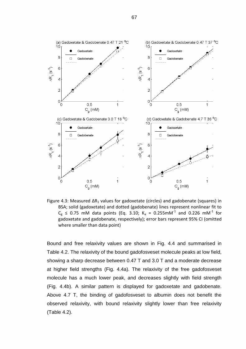
67

Figure 4.3: Measured ΔR1 values for gadoxetate (circles) and gadobenate (squares) in BSA; solid (gadoxetate) and dotted (gadobenate) lines represent nonlinear fit to Cg ≤ 0.75 mM data points (Eq. 3.10; Ka = 0.255mM-1 and 0.226 mM-1 for gadoxetate and gadobenate, respectively); error bars represent 95% CI (omitted where smaller than data point)

Bound and free relaxivity values are shown in Fig. 4.4 and summarised in

Table 4.2. The relaxivity of the bound gadofosveset molecule peaks at low field,

showing a sharp decrease between 0.47 T and 3.0 T and a moderate decrease

at higher field strengths (Fig. 4.4a). The relaxivity of the free gadofosveset

molecule has a much lower peak, and decreases slightly with field strength

(Fig. 4.4b). A similar pattern is displayed for gadoxetate and gadobenate.

Above 4.7 T, the binding of gadofosveset to albumin does not benefit the

observed relaxivity, with bound relaxivity slightly lower than free relaxivity

(Table 4.2).

68

Figure 4.4: Calculated bound (left column) and free (right column) relaxivity values for all three agents, split by temperature (labelled 21 °C and 37 °C, but actual temperatures may differ slightly – see Table 4.1); error bars represent 95% CI (omitted where smaller than data point)

69

Table 4.2: Summary of calculated relaxivity values and 95% confidence intervals (mM-1 s-1)

The influence of additional binding sites is illustrated for gadofosveset in

Fig. 4.5, where the original model is adapted to include second and third

binding sites (Eq. 4.3a–c). Model fitting results are shown at room temperature

only; body temperature model fits (Appendix B (Fig. B.2)) display a very

similar pattern.

Gadofosveset 21 °C 37 °C 21 °C 37 °C 19 °C 37 °C 22 °C 33 °C

r1bound 33.4 (1.2) 42.4 (2.9) 12.0 (1.4) 8.4 (0.5) 7.4 (0.6) 5.3 (0.4) 4.6 (0.8)

r1free 8.9 (0.3) 6.6 (0.2) 8.7 (0.2) 7.1 (0.5) 5.1 (0.3) 6.5 (0.2) 5.3 (0.1)

r1obs 26.1 (4.2) 31.8 (4.6) 11.0 (0.4) 8.0 (0.2) 6.7 (0.1) 5.7 (0.5) 4.8 (0.5)

Gadoxetate 21 °C 37 °C 18 °C 36 °C

r1bound 27.2 (1.5) 30.9 (0.7) 11.8 (2.9) 4.6 (1.0)

r1free 7.2 (0.2) 5.5 (0.1) 7.4 (0.2) 5.2 (0.3)

r1obs 9.9 (0.4) 9.0 (0.3) 8.0 (0.4) 5.1 (0.1)

Gadobenate 21 °C 37 °C 18 °C 36 °C

r1bound 33.9 (1.2) 39.5 (1.2) 13.7 (0.4) 5.6 (9.0)

r1free 5.7 (0.1) 4.3 (0.1) 5.7 (0.1) 3.6 (0.1)

r1obs 9.2 (0.1) 8.7 (0.1) 6.7 (0.1) 3.8 (1.1)

0.47 T 3.0 T 4.7 T 9.4 T

70

Figure 4.5: Modelling n = 1 – 3 binding sites at all field strengths at room temperature, using Eq. 4.3a–c. Circles represent measured gadofosveset data points; solid line is original model (single binding site, Eq. 4.3a, Ka1 = 11.0 mM-1); dotted line also includes a second binding site (Eq. 4.3b, Ka2 = 0.86 mM-1); dashed line also includes a third binding site (Eq. 4.3c, Ka3 = 0.26 mM-1); the same relaxivity values (from Table 4.2) were used at all three binding sites

A comparison of measured R1 values for gadofosveset in BSA (at

Csa = 0.67 mM) and in mouse plasma at body temperature is shown in Fig. 4.6.

71

Figure 4.6: Comparison of R1 values at 37 °C for gadofosveset in BSA (circles, Csa = 0.67 mM) and in mouse plasma (squares) at (a) 0.47 T and (b) 4.7 T

4.6 DISCUSSION

4.6.1 Relaxation rates

Gadofosveset

The relationship between R1 and Cg for gadofosveset in the absence of

albumin is approximately linear, with any differences caused by field strength

only being observed at very high Cg (Fig. 4.1a). For gadofosveset in the

presence of albumin, a nonlinear relationship between R1 and Cg is observed

(Fig. 4.1b).

Applying the nonlinear ΔR1 model (Eq. 3.10) to the BSA measurements at low

Cg (≤ 0.75 mM), it is clear that the model underestimates ΔR1 at high Cg at

0.47 T (Fig. 4.2a). This underestimation at high Cg is likely to be due to the

assumption of a single binding site. Once this binding site is filled for all

albumin molecules (at Cg = Csa), additional gadofosveset is assumed to remain

free. However, if gadofosveset also binds to other sites on the albumin

molecule, this may lead to a greater contribution to observed ΔR1. The

underestimation is not observed at higher fields (Fig. 4.2b to 4.2d), where the

72

differences between relaxivities of the bound and free molecule are expected to

be small. As can be seen from Eq. 3.10, when r1bound approaches r1free the ΔR1

calculation is dominated by the product of r1free and Cg and the model becomes

approximately linear.

Gadoxetate and gadobenate

For both gadoxetate and gadobenate in PBS, there is no difference between R1

at 0.47 T and 3.0 T (Fig. 4.1c and 4.1e). In the presence of albumin,

gadoxetate ΔR1 values are slightly higher than equivalent gadobenate values

(Fig. 4.3); there is some evidence of nonlinearity in these plots at 0.47 T, but

the plots at higher fields are approximately linear.

4.6.2 Relaxivity

Gadofosveset

At 0.47 T, the r1free, r1bound and r1obs values at 37 °C in this study (6.6, 42.4 and

31.8 mM-1 s-1, respectively) are close to those found in the literature

(r1free = 6.8 mM-1 s-1 (162), r1bound = 42 mM-1 s-1 (approximately, below

Cg = 1 mM) (68) and r1obs = 28.0 mM-1 s-1 (91)). r1free and r1obs values at 4.7 T at

37 °C are also close to literature values (5.1 and 6.7 mM-1 s-1, respectively, in

this study versus 5.5 and 6.9 mM-1 s-1, respectively, in the literature (91)). Due

to variations in experimental set-up, it is difficult to find directly equivalent r1bound

literature values for comparison at field strengths of 3.0 T and above.

Bound (and observed) gadofosveset relaxivity at 0.47 T has previously been

shown to increase with temperature, with free relaxivity decreasing with

temperature (37). This pattern is also demonstrated at 0.47 T in this study

(Fig. 4.4). At high field, r1free remains consistently lower at 37 °C than at 21° C

(Fig. 4.4b), but r1bound values at high field are very similar for both temperatures

(Fig. 4.4a). Although the heating mechanism used at 9.4 T was unable to heat

73

the samples above 34 °C, it is likely the results would have been very similar

at 37 °C.

Gadoxetate and gadobenate

Calculated free relaxivity values at 0.47 T and 4.7 T for gadoxetate and

gadobenate (Fig. 4.4d and 4.4f; Table 4.2) closely match those published

elsewhere (91), although comparative bound relaxivity values are more difficult

to find in the literature. Studies of gadobenate at 0.47 T and 37 °C have

calculated r1bound at 36 mM-1 s-1 in rabbit plasma (78), and 32 mM-1 s-1 (163)

and 42.9 mM-1 s-1 (126) in human serum albumin. These values are close to

the equivalent gadobenate r1bound value of 39.5 mM-1 s-1 in this study. Also at

0.47 T and 37 °C, r1bound for gadoxetate in human serum albumin has been

calculated at 37.3 mM-1 s-1 (126), compared with a value of 30.9 mM-1 s-1 in this

study.

Calculated r1bound values are lower, and r1free and r1obs values are slightly higher,

for gadoxetate than gadobenate across all fields and temperatures. This is

generally consistent with values reported elsewhere (91).

4.6.3 Multiple binding sites

As illustrated in Fig. 4.2a, at low field the nonlinear model underestimates

gadofosveset ΔR1 at high Cg. This is likely to be due to the influence of

additional binding sites on the albumin molecule not accounted for by the

model. Eq. 3.10 is derived based on the assumption of a single bound

gadofosveset molecule per serum albumin molecule, with a saturation point at

Cg = Csa. If gadofosveset were to bind at multiple sites on the albumin

molecule, saturation would occur at a higher Cg (> Csa). A modified version of

Eq. 3.10 accommodating n binding sites of equivalent affinity (Eq. 3.11 in

Chapter 3) has previously been presented in the context of gadofosveset

relaxation rates (37, 77). However, the primary binding site has been shown to

have a substantially higher binding affinity than other sites (11.0 mM-1 at the

74

primary site, compared to 0.84 and 0.26 mM-1 at the second and third binding

sites, respectively (68)), therefore this approach may not be applicable. It is

unclear to what extent these additional bound molecules influence the overall

relaxivity. A similar relaxivity at all binding sites has previously been assumed

(164), although it is suggested that the primary binding site is one of higher

relaxivity (68).

An alternative model to accommodate up to three binding sites is suggested

(Eq. 4.3). Three versions of the model are plotted in Fig. 4.5 to assess

differences between inclusion of one, two and three binding sites, along with

measured gadofosveset data points at all field strengths and temperatures. All

models use the appropriate r1free value from Table 4.2. As bound relaxivities at

the second and third sites are not known, all bound relaxivities were set to the

same value (r1bound1 = r1bound2 = r1bound3 = r1bound from Table 4.2).

At 0.47 T, the underestimation of ΔR1 at high Cg noted in the original model

(solid line, Fig. 4.5a) is improved by the inclusion of a second binding site

(dotted line), but values at high Cg are overestimated by the inclusion of a third

binding site (dashed line). This overestimation for n = 3 is likely to be due to the

same r1bound value being used for all three sites; in reality, it may be that r1bound1

> r1bound2 > r1bound3. Additional binding sites provide minimal improvement to the

model fit at 3.0 T; at higher fields the difference is negligible and the

consideration of additional binding sites may be unnecessary. In vivo, the

consideration of additional binding sites is unlikely to be a factor during the

post-bolus equilibrium phase (where Cg values are lower). The requirement to

consider multiple binding sites may be eliminated altogether if the peak Cg

value is sufficiently low, which may be achieved by reducing the dose or

injection rate, for example.

A previous study using ultrafiltration showed that gadoxetate and gadobenate

interacted with albumin at a single site (126), and no published binding affinity

values can be found for a second binding site. The model fits well with a single

site (Fig. 4.3); adding a second binding site (with an equal affinity to the first

site) does not improve the model fit (see Appendix B (Fig. B.3)).

75

4.6.4 Species differences: gadofosveset

All measurements of bound relaxivity for gadofosveset were made using bovine

serum albumin at a concentration of 0.67 mM (4.5% w/v). As mentioned in

section 3.1.2, the variation in the bound fraction of gadofosveset between

species is thought to be mostly attributable to differences in albumin level,

therefore assessing in vitro gadofosveset samples containing albumin at a level

corresponding with that found in humans should ensure the results are relevant

for potential clinical translation.

Confirmation of the dominant influence of bound fraction is found not only in the

comparison of observed relaxivity between gadofosveset and gadoxetate or

gadobenate, but also in the measurements of gadofosveset in mouse plasma.

Here, relaxation rates for gadofosveset in mouse plasma at Cg ≤ 2 mM were

compared with values using BSA at Csa = 0.67 mM at low (0.47 T) and high

(4.7 T) field (Fig. 4.6). The difference in R1 between BSA and mouse plasma is

significant at 0.47 T (Fig. 4.6a), where bound fraction has a much greater

influence over the observed relaxivity due to the large difference between

r1bound and r1free (Table 4.2). At 4.7 T, there is little difference between BSA and

mouse plasma R1 measurements (Fig. 4.6b), reflective of the small difference

between r1bound and r1free at high field, resulting in a lower influence of bound

fraction on observed relaxivity.

4.6.5 Limitations

The one-parameter model used to determine r1bound by fitting to experimental

ΔR1 values (Eq. 3.10) assumes a fixed literature value for Ka. An attempt was

made to derive Ka rather than take a literature value, by fitting Eq. 3.10 for two

unknown parameters. However, this revised model could not be satisfactorily

resolved (returning Ka and r1bound values beyond the range that might

reasonably be expected). The influence of Ka may be explored by comparing

the model fit at additional Ka values; doubling or halving the assumed Ka value

76

of 11.0 mM-1 does not significantly alter the model fit at 0.47 T in this study

(Fig. 4.7), and would have even less effect at higher fields. Although some

difference in binding affinity may be expected between room and body

temperature, a constant Ka value was used at both temperatures as only

relevant literature Ka values at 37 °C could be found.

Figure 4.7: Effect of Ka on gadofosveset model fit at 0.47 T at (a) 21 °C and (b) 37 °C; data points and solid lines match those in Fig. 4.2a and 4.2b

A second potential limitation of this study is that bovine serum albumin was

used as a surrogate for human serum albumin. Although the binding

characteristics of BSA may differ slightly from those of HSA, albumin solutions

were created at a typical concentration expected in healthy humans, therefore

bound fractions and the proportional influence of the bound and free

gadofosveset molecule on observed relaxivity would still be expected to be

applicable. Bovine plasma has previously been used as the solvent for

assessing the relaxivities of a range of contrast agents (91). BSA has been

shown to be similar in structure to HSA, with some differences in binding

pockets (165).

As noted in Chapter 2 (Table 2.1) the standard clinical dose for gadobenate is

0.1 mmol kg-1, which is higher than gadoxetate (0.025 mmol kg-1) or

gadofosveset (0.03 mmol kg-1). In this study like-for-like concentration

comparisons were made (up to 1 mM), and no account was taken of the

variation in clinical dose between agents. The physiologically applicable

77

concentration range could have been extended for gadobenate, although the

results as presented remain valid.

For various reasons (time constraints, faulty or unavailable heating

mechanisms) it was not possible to acquire data for all contrast agents at all

fields at room and body temperature. As gadofosveset is the main focus of this

research, priority was given to acquiring data for this agent. Although the

dataset is incomplete, the influence of temperature on the relaxivity of the

bound and free molecule is clearly observed. Any small variation in ‘room’ or

‘body’ temperature between agents is unlikely to have a significant impact on

the conclusions drawn from the results as presented.

4.6.6 Summary

In summary, this study provides information regarding gadofosveset

longitudinal relaxivity not currently available elsewhere, particularly in relation to

bound relaxivity values at field strengths of 3.0 T and above. Differences

between the longitudinal relaxivities of the bound and free gadofosveset

molecule are large at low field but small at high field. Factors influencing the

bound fraction, such as relative concentrations of gadofosveset and serum

albumin, will therefore have a significant impact on the observed relaxivity at

low field but will have limited impact at high field. Consideration should be given

to incorporating a dynamic relaxivity, which changes with bound fraction, when

applying tracer kinetic models at low field. The influence of species differences

in albumin levels and binding properties is demonstrated to have a much

greater effect at low field, and may markedly alter the outcome of pre-clinical

studies using gadofosveset. The common assumption that a single

gadofosveset molecule binds per albumin molecule may lead to an

underestimation of relaxation rate at low field at high gadofosveset

concentration, although this model simplification has little influence at

high fields.

As expected from the literature, bound and free longitudinal relaxivities for

gadoxetate and gadobenate are generally similar to those for gadofosveset.

78

However, due to a much lower binding affinity, the observed relaxivity is

significantly lower for these agents than for gadofosveset at low field. As with

gadofosveset, bound relaxivity values calculated here for gadoxetate and

gadobenate at field strengths of 3.0 T and above have not previously been

published. As field strength increases, r1bound approaches r1free at high field and

the influence of binding on observed relaxivity reduces, although even at low

fields the change in relaxation rate with contrast agent concentration is

approximately linear. The use of any contrast agent in quantitative MRI studies

requires an accurate relaxivity value to precisely monitor contrast agent

kinetics. The in vivo relaxivity of an albumin-binding contrast agent is dynamic

rather than fixed, varying particularly during the first bolus pass when the bound

fraction is changing rapidly. The data presented here for gadoxetate and

gadobenate suggests that, unlike gadofosveset, a single relaxivity value may

still adequately represent this situation due to the relatively low binding affinity

of these agents.

It should be noted that only the longitudinal relaxivity properties of these

albumin-binding agents have been explored in this chapter. Transverse

relaxivity measurements are discussed in Chapter 7, and may provide an

alternative approach to utilising these agents in dynamic contrast-

enhanced studies.

79

CHAPTER 5: A THEORETICAL APPPROACH TO IN VIVO

GADOFOSVESET BLOOD CONCENTRATION MEASUREMENT

5.1 BACKGROUND

5.1.1 Contrast agent blood concentration

Establishing the blood concentration of a contrast agent is a fundamental step

in calculating many quantitative parameters in dynamic contrast-enhanced

(DCE) MRI. DCE-MRI enables functional tissue parameters to be assessed by

monitoring the transit of a contrast agent over time. Amongst its many areas of

application, DCE-MRI has been used in the quantitative assessment of

myocardial (166) and pulmonary (167) perfusion. DCE-MRI may also be used

to assess angiogenesis, a process that is fundamental to the progress and

metastasis of tumours, along with other biomarkers in oncology (168).

Quantification may be based on a simple, non-model-based approach such as

measuring enhancing fraction (20). Charting signal intensity against time

provides tissue-related parameters including onset time, maximum signal

intensity and wash-out characteristics (23).

Alternatively, parameters such as tissue perfusion and micro-vessel

permeability may be determined through the application of tracer kinetic

models. Commonly, these models consist of two compartments representing

intravascular and extravascular extracellular spaces, with the rate of transfer

between the compartments determined through mathematical modelling (169).

The conventional starting point for such models is the intravascular contrast

agent concentration prior to extravasation, known as the vascular input function

(VIF), which can be measured in a nearby vessel (170). In such models,

quantitative parameters are derived by separating changes in contrast agent

80

concentration within the tissue of interest from those in a feeding artery using

deconvolution (171).

The VIF following bolus injection of a gadolinium (Gd) contrast agent is

characterised by a high initial peak in contrast agent concentration during the

wash-in phase, of very short duration, followed by a decrease in concentration

during the wash-out and clearance phases. Often, the VIF is modelled as either

an instantaneous peak or a sharp linear rise to peak concentration, followed by

a bi-exponential decay representing extravasation and excretion rates

(Fig. 5.1). This simplified approach neglects potential recirculation effects; more

complex models attempt to correct for this (172).

Figure 5.1: Example of a VIF, showing linear rise to peak and bi-exponential decay (not accounting for recirculation effects) ((173), using parameters from (172))

The robustness of tracer kinetic models may be compromised by practical

difficulties associated with accurate VIF measurement. Potential errors in

converting measured signal intensity to contrast agent concentration may be

further complicated when using gadofosveset, due to its binding to albumin,

and may be exacerbated by acquisition limitations including temporal

resolution, signal saturation, partial volume effects and flow artefacts (174), and

by delay and dispersion of the bolus in the tissue of interest (26). In small

animals, the requirement for improved spatial resolution due to smaller vessel

size must compete with an increased temporal resolution requirement due to a

81

higher heart rate (175-177). Using a population average VIF, rather than one

acquired from an individual subject, may improve model robustness (178),

particularly in small animals (179). An alternative approach to measuring

vascular signal intensity changes may be to take measurements in a reference

tissue within the field of view (180).

Laboratory analysis of ex vivo blood samples eliminates the requirement for

signal intensity conversion, and may be considered the gold standard measure

of contrast agent concentration in the blood. In humans, good agreement has

been shown between VIF curves plotted from blood sample measurements and

those using MRI signal intensities following injection of gadopentetate (181).

However, using blood sampling techniques to capture the first pass of a bolus

injection of contrast agent can be challenging due to the requirement for

multiple blood samples in a short time-frame. Limitations regarding permissible

sampling volumes add further difficulty in studies using small animals, although

a recent study in rats found a good correlation between VIF descriptors

calculated from measurement of Gd concentration in blood samples with those

determined using imaging techniques (182).

5.1.2 Blood sampling

Blood sampling is one of the most commonly performed procedures in animal

studies (183), and is fundamental to the success of pharmacokinetic and

toxicology studies. Blood should always be collected in the manner that gives

least pain and stress (184), and the amount of blood taken on a single occasion

should not exceed 10% of circulating blood volume to prevent hypovolaemic

shock (185). In a small mammal such as a mouse, this blood sampling volume

limit may be less than 200 μL (79).

Micro-sampling, the removal of less than 100 μL, causes less subject

interference than conventional sampling (186). Blood micro-samples are often

acquired with capillary tubes, and are then either centrifuged to produce

plasma or analysed directly as whole blood. Direct analysis requires an

82

accurate blood sample volume and precise, low-temperature storage

conditions, and may occasionally result in clotting within the micro-tube

(although using EDTA-coated tubes avoids clotting). Preparation of plasma

samples also requires an accurate volume and restrictive storage conditions,

with additional handling steps to remove the red blood cells.

An alternative micro-sampling technique, dried blood spotting (DBS), removes

the requirements for accurate blood sample volume and low-temperature

storage. It is a widely accepted blood sampling technique for individual testing

and population screening. A DBS card usually consists of four circular regions

(each 10 mm in diameter), within which blood volumes of around 10 – 30 μL

are spotted (Fig. 5.2). The cards are dried at room temperature for two hours

before being sealed in an airtight bag with desiccant sachets and stored at

room temperature until required. A punched core of 3 – 6 mm diameter from

each spot, equating to a blood volume of approximately 3 – 12 μL (187), is then

placed in an extraction solution prior to spectral analysis.

Figure 5.2: Transferring blood to DBS card (image from Whatman web site (188))

The DBS technique has been actively used since Robert Guthrie’s pioneering

work in the 1960s for screening new-born babies for metabolic anomalies such

as phenylketonuria and congenital hypothyroidism (189). More recently, it has

also been used for early detection of a range of diseases including cystic

fibrosis (190) and the hepatitis C virus (191). DBS is considered a stable,

inexpensive method of collecting and storing DNA for epidemiological

studies (192).

83

Advantages of DBS over conventional blood sampling techniques include ease

of collection and economical storage (samples are stored at room temperature,

rather than in a freezer). As the samples remain stable at room temperature,

they can be collected at remote locations and posted to a central laboratory for

analysis. DBS also requires smaller collection volumes, which increases the

number of potential data points per experimental animal and facilitates the

reduction in animal numbers required for preclinical studies (193). Serial

sampling from a small number of animals also has the advantage of reducing

the influence of inter-animal variability.

5.1.3 Measuring Gd content

Inductively-coupled plasma mass spectrometry (ICP-MS) is one of a range of

spectrometry techniques available to analyse blood samples. It is a highly

sensitive element-detection technique, commonly used by the pharmaceutical

industry for identification of inorganic impurities at levels as low as parts per

trillion (194) and with many applications in a wide variety of industries including

food quality assessment and environmental monitoring (195). ICP-MS has

been utilised as a means of monitoring environmental Gd levels and measuring

tissue Gd accumulation, resulting directly from the use of MRI contrast agents

(196). It has also been adopted as the gold standard for measurement of Gd

content in several in vitro studies characterising gadofosveset (for example,

(68, 75)).

A schematic diagram of the ICP-MS process is shown in Fig. 5.3, and an

illustration of the key components is given in Fig. 5.4. The process begins with

a liquid sample, pumped into the mass spectrometer and nebulised into an

aerosol by a stream of argon gas within the spray chamber. Large drops are

drained by gravitational force, with only small drops (up to a diameter of 10 μm)

continuing to the sample injector. Utilising pressure gradients, the aerosol is fed

into a plasma torch, where argon gas is converted to a plasma discharge and

heated to a maximum of 7000 K by a radiofrequency (RF) coil. As the liquid

aerosol travels through different temperature zones within the plasma, it dries

84

and becomes a solid, and is vaporised into molecular and then atomic form.

When the sample reaches the extremely hot centre of the plasma, there is

sufficient energy in the plasma electrons to knock an electron from the outer

orbit of the sample atoms. The resulting positively charged ions are driven into

the analyser through a sample and skimmer cone, which are maintained within

a vacuum, and then focused and steered by ion lenses through to a quadrupole

mass separation device. This device consists of two pairs of rods, one pair with

a direct current (DC) field and the other pair with an RF field. Selecting the

appropriate RF–DC voltage enables the operator to tune the device to allow

only ions of a specific mass-to-charge ratio to pass down the middle of the

rods, with other ions falling through gaps between the rods and being ejected.

The selected ions finally reach the ion detector, where they are counted and a

mass spectrum is created.

Figure 5.3: Schematic diagram showing the steps in the process of ICP-MS

Nebulisation

Desolvation

Vaporisation

Atomisation

Ionisation

Mass analysis

Liquid sample

Aerosol

Particle

Molecule

Atom

Ion

Spectrum

85

Figure 5.4: Key components in an inductively-coupled plasma mass spectrometer (not to scale); sample movement in diagram is from right to left

To prevent signal saturation and accumulation of particulate matter, it is

important that samples are diluted and large molecules broken down prior to

being pumped into the spectrometer. Whole blood samples containing Gd-

based MRI contrast agents have previously been analysed with ICP-MS, using

20% v/v nitric acid as the digestion agent. An acid content at this level is very

effective at releasing Gd, and nitric acid is noted to be the best acid medium for

ICP-MS (197). Concentrations should be above the detection limit, i.e.

sufficiently high to be distinguishable from system noise, but should not be so

high as to saturate the ion counter. A detection limit has previously been

measured for Gd at 1 ng mL-1 (198).

Pilot studies have been carried out to assess the validity of combining DBS with

ICP-MS to screen for heavy metal environmental pollutants such as lead,

mercury and cadmium in new-born babies (199). The study concluded that this

was a useful screening method, and also found that samples remained stable

when stored over an 8.5 month period. Another study on levels of lead in the

blood was carried out using laser ablation to create particulates directly from

DBS cores, followed by ICP-MS analysis (200).

A literature search (May 2013) found no previous studies using DBS to

measure Gd concentration. Although a similar technique to ICP-MS,

inductively-coupled plasma atomic emission spectroscopy (ICP-AES), has

86

previously been used to measure blood concentrations of gadofosveset in

rabbits following bolus injection (78), the blood sampling volumes used would

be inappropriate for smaller animals. An aforementioned study in rats (182)

used ICP-MS to measure the Gd content of blood samples following injection of

gadopentetate, although blood sampling volumes are not stated. To

successfully measure the gadofosveset time course in a mouse model, the

novel combination of micro-sampling mouse blood using DBS followed by Gd

measurement using ICP-MS is suggested.

5.2 AIMS

The aim of this study was to combine the established techniques of DBS and

ICP-MS to develop a method for accurate measurement of the Gd content of

blood samples at a temporal rate suitable for characterising a VIF in small

mammals. This would be achieved in three steps:

1. Demonstrate in a proof-of-concept study that Gd levels could be accurately

measured using ICP-MS with gadofosveset-spiked mouse blood samples on

DBS cards. By plotting Gd counts against known Gd concentrations, calibration

curves could then be created to enable conversion of Gd counts back to Gd

concentrations. Applying a linear fit to these plotted data points enables

assessment of the accuracy of the calibration method.

2. The method developed in vitro could then be applied in a benchtop

experiment by injecting several mice with a standard dose of gadofosveset,

collecting blood samples on DBS cards at specific, interleaved time points and

analysing these samples for Gd using ICP-MS. These Gd counts would be

converted to Gd concentrations using the calibration curves generated from the

in vitro data, and Gd concentrations could be plotted as a VIF.

3. Using the same injection protocol as the benchtop experiment, MR images of

mice would be acquired at corresponding time points. The measured variation

87

in signal intensity within a major vessel as the injected bolus makes its first

pass through the animal could then be compared with the previously

acquired VIF.

There are two novel aspects to this study: firstly, the use of DBS in conjunction

with ICP-MS to facilitate accurate Gd measurement in low-volume blood

samples; and secondly, the application of this combined technique to determine

a VIF for gadofosveset in a murine model. As gadofosveset was withdrawn

from the European market before the animal studies commenced, only the in

vitro method development stage could be completed. Although it would have

been feasible to use an alternative Gd-based contrast agent to assess the

method in vivo, the primary research purpose of this project is characterisation

of gadofosveset. As gadofosveset has unique properties not found in other

clinically approved agents, the option to complete the in vivo assessment with

another contrast agent was rejected on ethical grounds.

5.3 METHOD

To separately validate the accuracy of Gd measurement using ICP-MS and the

method for releasing Gd from DBS card, three sets of ICP-MS calibration

curves were created. The first set of curves used gadofosveset in mouse

plasma, directly prepared in solution form (without being transferred to DBS

cards), to verify that Gd content could be accurately measured with the chosen

diluent and dilution levels. The second set of curves used solutions of

gadofosveset in phosphate-buffered saline (PBS), transferred to DBS cards

and prepared for ICP-MS, to confirm that unbound gadofosveset would be

released from the card and Gd content could be accurately measured. The

third set of curves used mouse blood samples spiked with gadofosveset,

transferred to DBS cards and prepared for ICP-MS, to confirm that bound

gadofosveset would be released from the card and Gd content could be

accurately measured at low blood volumes. This final set of curves would have

88

been used to convert Gd counts in ex vivo blood samples to Gd concentrations

if an animal benchtop experiment had been carried out.

5.3.1 Sample preparation

Gadofosveset (Vasovist) at an initial concentration of 250 mM (244 mg mL-1)

was added to lyophilised mouse plasma (reconstituted with deionised water) to

give a concentration of 5.0 mM. This was serially diluted to give additional

concentrations of gadovosveset in mouse plasma of 2.0, 1.0, 0.5 and 0.25 mM

(a range of 0.24 – 4.88 mg mL-1), along with a sample of mouse plasma without

gadofosveset. 10 μL of each solution was then diluted by a factor of 104 in nitric

acid (20% v/v) to give final sample concentrations in the range

24 – 488 ng mL-1.

To generate the DBS samples, gadofosveset was diluted in phosphate-buffered

saline (PBS, as used in Chapter 4 experiments) to a concentration of 15 mM,

followed by serial dilutions in PBS to give concentrations of 6, 3, 1.5 and

0.75 mM. 50 μL of each of these solutions was added to 100 μL mouse blood

(CD-1 mouse type) to give final concentrations of 5, 2, 1, 0.5 and 0.25 mM

(0.24 – 4.88 mg mL-1). An equivalent set of concentrations for gadofosveset in

PBS (without blood) was also created. EDTA-coated 20 μL capillary tubes

(Starstedt AG, Germany) were used to draw samples from each gadofosveset–

blood and gadofosveset–PBS solution and spot onto Whatman FTA DMPK-C

cards (GE Healthcare). An additional card containing spots of plain mouse

blood was also created. The cards were stacked horizontally in a drying rack

for 2 h at room temperature (approximately 22°C, with a measured relative

humidity of 36%). Each card was then sealed in an airtight bag containing two

desiccant sachets and stored at room temperature until use.

To prepare the DBS samples for ICP-MS analysis, a single 3 mm diameter

punched core from the centre of each spot was placed into a plastic Eppendorff

tube (0.5 mL) and 200 μL nitric acid (20% v/v) added. The tubes were vortexed

for 20 s, left to stand for 40 min and then centrifuged at 5000 rpm for 5 min.

89

200 μL of supernate was extracted to a plastic Corning tube (15 mL), 1980 μL

of nitric acid (20% v/v) added and the combined solution vortexed for 5 s prior

to ICP-MS. Assuming a blood volume in the core of approximately 3 μL, this

overall process amounts to a dilution from the original blood concentration

levels of approximately 1 in 6,800, giving final concentrations in the range

37 –732 ng mL-1. Coring took place four days after samples were spotted on

the DBS cards.

5.3.2 ICP-MS

ICP-MS was carried out on an Elan DRC-e spectrometer (Perkin Elmer,

Waltham, MA) with quadrupole mass analyzer, peristaltic pump and pneumatic

concentric nebulizer, using argon gas. Counts were determined for the four

most commonly occurring isotopes of Gd (mass/charge values of 156, 157, 158

and 160), which account for around 83% of the stable element (201). A sample

flush of 35 s at 24 rpm was followed by a read delay of 35 s at 20 rpm and a

wash with 0.1% (v/v) nitric acid of 60 s at 30 rpm.

5.4 RESULTS

Figures 5.5, 5.6, and 5.7 show the calibration curves for gadofosveset in mouse

plasma (solution form), gadofosveset in PBS (DBS core extraction) and

gadofosveset in mouse blood (DBS core extraction), respectively. All three sets

of plots show a high degree of linearity between gadofosveset concentration

and Gd count, with R2 values exceeding 0.998 for all plots.

90

Figure 5.5: Calibration curves showing Gd counts (mass/charge values of 156, 157, 158 and 160, and the total count for all four) for a range of gadofosveset concentrations in mouse plasma, using samples taken from in vitro solutions; error bars indicate standard deviation of four measurements. R2 values for all plots ≥ 0.999

91

Figure 5.6: Calibration curves showing Gd counts (mass/charge values of 156, 157, 158 and 160, and the total count for all four) for a range of gadofosveset concentrations in PBS, using DBS collection method. R2 values for all plots ≥ 0.998

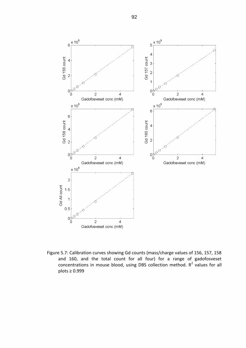
92

Figure 5.7: Calibration curves showing Gd counts (mass/charge values of 156, 157, 158 and 160, and the total count for all four) for a range of gadofosveset concentrations in mouse blood, using DBS collection method. R2 values for all plots ≥ 0.999

93

5.5 DISCUSSION

5.5.1 Method validation

The high degree of linearity between gadofosveset concentration and Gd count

for the in vitro solutions of gadofosveset in mouse plasma (Fig. 5.5), diluted by

a factor of 104, confirms that ICP-MS is a very sensitive method for measuring

Gd concentration. These results also show that the extraction solution and

dilution methodology are valid preparation for ICP-MS measurement. The

additional methodology for releasing samples from DBS cores and creating

liquid solutions is validated initially for gadofosveset in PBS (Fig. 5.6), where no

gadofosveset binding will occur, and subsequently for gadofosveset in mouse

blood (Fig. 5.7), where the majority of the gadofosveset will be bound to

albumin. The linearity of both sets of plots suggests that this method

adequately releases Gd from the DBS core, regardless of albumin-binding

state. The consistency between samples prepared in solution form and those

prepared from DBS cores demonstrates that the preparation method used to

generate solutions from blood samples on DBS cards was appropriate for

ICP-MS analysis. Overall, the results demonstrate the viability of using blood

samples acquired and stored on DBS cards in conjunction with ICP-MS to

measure Gd levels. This suggests the method may be a viable, accurate

means of monitoring Gd concentrations in the blood (ex vivo) following contrast

agent administration.

ICP-MS has previously been used to measure Gd from MRI contrast agents in

tissue and environmental samples (196). The technique was found to be highly

sensitive to Gd in rat tissue, with a detection limit of approximately

6 x 10-6 μmol of Gd per g of tissue (197). Concern around the build-up of Gd in

tissue has increased with the establishment of a link between Gd contrast

agent administration and nephrogenic systemic fibrosis (NSF) (49); a study

using ICP-MS to measure Gd in hair, fingernail and blood samples of an NSF

patient previously exposed to Gd contrast agents (202) found substantially

higher Gd levels than in healthy control subjects. ICP-MS has also been used

94

to study the elimination time course of Gd from the skin in rats in the days

following administration of a range of contrast agents (203, 204). Recently, the

VIF in a rat model was captured using ICP-MS by blood sampling after injection

of gadopentetate, and was reproduced with an MRI sequence (182). Tissue

distribution for gadopentetate has also been assessed in rats using laser

ablation ICP-MS on histological samples (205). ICP-MS has been used to

assess levels of Gd passing through hospital sewage systems into rivers

following excretion by patients injected with Gd-based contrast agents during

MRI procedures (198, 206). The potential to differentiate specific Gd chelates

has been demonstrated using ICP-MS in conjunction with size-exclusion

chromatography (207) and hydrophilic interaction chromatography (208).

ICP-MS was used in a murine study to correlate histological tissue Gd

concentration in cardiac slices with change in relaxation rate (ΔR1) (209). A

study combining MRI, ICP-MS and histology assessed the clearance rate of a

macromolecular contrast agent (albumin-Gd-DTPA) in mice following avadin

chase (210), although the sampling intervals were insufficient to capture the

first bolus pass.

Several studies characterising gadofosveset in vitro (for example, (68, 75))

have used ICP-MS Gd measurements following solution filtration to determine

the binding fraction for physiologically relevant gadofosveset concentrations

across selected animal species. A study in rabbits (78) used ICP-AES to

analyse acquired blood samples at multiple time points immediately following

injection of gadofosveset. A total of 44 samples, each of volume 300 μL, were

acquired for a single animal, amounting to a total blood sample volume of

approximately 13 mL (around 8% of the total circulating blood volume of a

2.5 kg rabbit); these blood sample volumes would be unsuitable for a smaller

animal.

Blood sampling using DBS cards requires smaller blood volumes and has

practical advantages over other micro-sampling techniques (including ease of

sample handling, room-temperature transportation and storage of samples, and

the ability to store samples for several months without degradation). DBS may

be considered particularly useful for collection of blood samples in small

95

animals, where low circulating blood volumes prohibit multiple sampling at

conventional volumes. In line with the commitment to the welfare of animals

used in scientific experimentation (the ‘3Rs’ approach: replacement, reduction,

refinement, (211)), smaller individual blood sampling volumes facilitate the use

of fewer animals. In addition, acquiring multiple samples from the same animal

reduces the experimental risk of inter-animal variability.

5.5.2 Proposed in vivo validation methodology

Due to its withdrawal from the European market in 2011 (see Chapter 3,

section 3.1.1), it was not possible to validate the proposed method in vivo using

gadofosveset. As the primary research aim was characterisation of this contrast

agent, it was not considered ethical to carry out in vivo animal experiments

using another contrast agent. A suggested protocol for in vivo validation in a

murine model would involve two parallel experiments, subject to necessary

ethical approval and Home Office personal and project licence authorisation at

a designated establishment, in accordance with the Animals (Scientific

Procedures) Act 1986. In the first experiment, anaesthetised mice would be

injected with gadofosveset at the clinical dose (0.03 mmol kg-1), and blood

would be extracted to DBS cards at specific time points following injection.

Using the same injection protocol, the second experiment would involve

acquiring MR images at time points corresponding with those used for

blood sampling.

Assuming the animal is anaesthetised with isoflurane or an isoflurane/oxygen

mix, and gadofosveset is administered using a cannula in one of the tail veins,

the following blood extraction methodology is suggested. The first blood sample

is taken by needle pricking the non-cannulated tail vein, placing an EDTA-

coated 20 μL capillary tube on the site and allowing the blood to be drawn up

using capillary action. Although injection and sampling both use veins, this

should not be an issue due to the rapid rate at which blood circulates in small

mammals. Subsequent blood samples are taken from the same site; if

necessary, the flow of blood is stemmed between samples by applying

96

pressure to the sampling site. The capillary tubes are placed temporarily into

labelled Eppendorf tubes until all samples are collected for the animal. Taking

six blood samples per animal, the total captured blood volume per animal is no

more than 120 μL (approximately 7% of the total blood volume of a 20 g

mouse). The actual volume drawn into each tube by capillary action is likely to

be around 10 – 12 μL (60 – 72 μL total for six samples), plus a small amount of

wastage between samples. When all samples are collected for one animal, the

full volume of blood from each capillary tube is transferred to a DBS card. The

process is repeated for additional animals, using a range of time points, to build

up a full picture of the variation of contrast agent concentration with time.

Although laboratory mice are bred to give a similar physiological response, the

potential influence of inter-animal variability may be assessed by choosing a

combination of coincident and interleaved time points. DBS cards are allowed

to dry for two hours and then stored in airtight plastic bags with desiccant

sachets. The DBS core extraction method described in section 5.3 is then used

to prepare each sample for ICP-MS.

A log spacing of blood sample acquisition times is suggested, to provide a

greater number of data points soon after injection, where concentrations are

changing more rapidly. Fig. 5.8 gives a suggested distribution of sample times,

with 8 animals and 6 samples per animal. The total number of animals required

and the timing of blood sample acquisitions may be confirmed following a small

(n = 2) pilot study.

97

Figure 5.8: Proposed blood sampling times (6 time points for 8 animals), with the first time point immediately after a 30 s infusion; each symbol represents a different animal, with the same initial time point used for each animal

The MR imaging sequence should use cardiac and respiratory gating where

possible, and images should include a plane incorporating the aorta, vena cava

or ventricles, to enable accurate blood T1 measurement (175). As

deoxygenated haemoglobin is slightly paramagnetic, and the degree of

deoxygenation is 1 – 2% in arteries and 30 – 40% in veins (212), differences in

the vascular input function would be observed depending on whether the region

of interest incorporates venous or arterial blood.

5.5.3 Potential limitations

A potential limitation of the DBS method is the ability to acquire blood samples

rapidly enough to capture the first-pass peak contrast agent concentration.

There is also a requirement to generate consistent blood spot cores. The

volume of blood in a DBS core has been shown to vary with haematocrit levels

(213), overall volume of the blood spot (187) and with the relative positioning of

the core within the spot (214).

For ICP-MS, it is essential at very low Gd concentrations that measurements

exceed the limit of detection, the level above which a signal may be

98

distinguished from background noise, and the limit of quantification, the level

above which accurate measurement is possible. These levels may be

determined from the standard deviation of ion counts of solutions prepared

from blank cores. Although Gd concentrations in this study were well above

the expected detection and quantification limits, it may be of value in a

repeated experiment if Gd ion counts of blank solutions were recorded. False-

positive counts are possible when oxides matching the mass-to-charge ratio of

the isotope of interest are created during the ionisation process (from

combinations of elements within the sample solution and input gas), or as a

result of interference from other spectra. For example, isotopes of dysprosium

occur naturally (although rarely) at atomic masses of 156, 158 and 160.

99

CHAPTER 6: OVERCOMING THE LOW RELAXIVITY OF

GADOFOSVESET AT HIGH FIELD WITH SPIN LOCKING

6.1 BACKGROUND

The albumin-binding nature of gadofosveset, discussed in Chapter 3, leads to

reduced extravasation and excretion rates and potentially favourable relaxation

properties. Results from Chapter 4 (Table 4.2) confirm that the longitudinal

relaxivity of the bound gadofosveset molecule (r1bound) is significantly higher

than the relaxivity of the free molecule (r1free) at low fields. However, r1bound

decreases rapidly with field strength and the two relaxivities are comparable at

4.7 T (Chapter 4, Fig. 4.4). Where these relaxivities converge, observed

relaxivity (r1obs) is similar to that for a non-binding contrast agent and the high-

relaxivity advantage of gadofosveset is lost. Regardless of the reduction in

relaxivity, the unique kinetic properties of gadofosveset resulting from its

binding to albumin are displayed at all field strengths. An alternative contrast

mechanism that provides high gadofosveset relaxivity at high fields may be

required to fully exploit these properties.

Spin locking (SL), first described as an imaging technique in 1985 (15) but

investigated in NMR prior to this (215), involves the application of a 90°

excitation pulse followed by a radio frequency (RF) pulse (phase shifted by 90°

to the excitation pulse), applied for a duration of time (spin-lock time, TSL),

which locks the spins in the rotating frame of reference (Fig. 6.1).

100

Figure 6.1: (a) Magnetisation M0 is tilted 90° around x’ axis of rotating frame of reference x’y’z’ by excitatory pulse B1; (b) spin locking pulse B1L is applied along y’ axis

Relaxation of the magnetisation in the presence of this SL field (B1L) is

characterised by the time constant T1ρ, with free induction decay (FID) only

occurring once the spin-locking pulse has been switched off (Fig. 6.2a). The SL

pulse may be followed by a 90° pulse (phase shifted by 180° to the original

excitation pulse) and an imaging sequence (Fig. 6.2b) (216), or a 180° pulse

and readout (Fig. 6.2c) (15).

101

Figure 6.2: (a) Free induction decay follows the cessation of the spin-locking pulse; (b) an example of how an imaging sequence may be applied following spin locking (216); (c) a pulse sequence diagram showing spin-locking pulse followed by a selective 180° pulse and readout (15)

T1ρ is influenced by the strength of the SL field, which is commonly in the μT

(low kHz) range, rather than the main magnetic field (B0). As a result, the image

contrast generated by SL is equivalent to image contrast obtained at low

magnetic fields, with the advantage that a high signal-to-noise ratio, a

characteristic of high B0, may be maintained (217). It should be noted that the

SL RF pulse may contribute significantly to patient specific absorption rate

(SAR), particularly at high B0 as SAR is proportional to the product of B02, B1L

2

and the ratio of TSL to TR (within a practical range for TR) (Eq. 6.1) (15).

[6.1]

102

The interaction times associated with SL at very low field strengths give this

technique an increased sensitivity to proteins and other macromolecules (218).

This correlation between signal intensity and tissue protein has been utilised as

a potential biomarker for response to tumour therapy, including treatment

designed to reduce protein synthesis (219) and gene therapy resulting in

reduced protein content due to cell death (220). The clinical potential of SL has

also been highlighted in a study of injured myocardium (221) and in the

assessment of brain plaque composition in early-onset Alzheimer’s

disease (222).

Small-molecule Gd-based contrast agents have been used in combination with

SL to provide improved myocardium–blood contrast (221, 223) and in the

assessment of articular cartilage (224). SL after injection of gadopentetate has

also been shown to improve tumour contrast in glioma patients (218). A

literature search for published studies assessing the effect of gadofosveset on

T1ρ (July 2013) found only the paper on which this thesis chapter is

based (1).

Tissue T1ρ values fall between T1 and T2, with T1ρ → T2 as B1L → 0 (225).

Conventionally B1L << B0, therefore T1ρ may be expected to be close to T2. The

transverse relaxivity of bound gadofosveset is known to remain high at all

relevant field strengths (89), and T2 values are known to be sensitive to tissue

macromolecules (226). A secondary consideration in this study is whether the

potential benefits of T1ρ contrast could also be achieved using T2 contrast,

without the complication of adding a spin-locking pulse and without the

requirement to consider additional SAR factors.


The primary aim of this study was to test the hypothesis that by combining the

macromolecular sensitivity of SL with the albumin-binding affinity of

gadofosveset a large contrast shift may be achieved at field strengths where

the T1 effects of gadofosveset are very similar to those of conventional Gd-

103

based agents. In addition, the influence of species’ differences in binding on

spin-lock relaxation was investigated, along with the influence of spin-lock field

strength on image quality. A further aspect of the study was to investigate

whether the potential benefits of T1ρ contrast could also be achieved using T2

contrast. The following objectives were set:

1. Measure spin-lock relaxation rates (R1ρ, 1/T1ρ) for in vitro gadofosveset

solutions, in the presence and absence of serum albumin, at a B0 value of 4.7 T

and B1L values of 5, 25 and 90 µT.

2. Repeat R1ρ measurements for solutions of the non-binding contrast agent

gadopentetate dimeglumine, to act as a control and to separate the influence of

the macromolecular solution from that of Gd.

3. Repeat R1ρ measurements for gadofosveset in mouse plasma, to identify

differences between albumin species. This may be informative for translating

the outcome of pre-clinical studies utilising gadofosveset with spin locking.

4. Compare gadofosveset R1ρ measurements with equivalent R1

measurements presented in Chapter 4.

5. Measure R2 for gadofosveset in the presence and absence of albumin, at

low (0.47 T) and high (4.7 T) B0, to determine whether transverse relaxation

rates display a similar trend to spin-lock relaxation rates.

6.3 METHOD

6.3.1 In vitro solutions

In vitro solutions of gadofosveset in phosphate-buffered saline (PBS), with and

without bovine serum albumin (BSA), were prepared as described in Chapter 4

(section 4.4.1). An equivalent set of solutions of the non-binding contrast agent

gadopentetate dimeglumine (Magnevist, Bayer Healthcare Pharmaceuticals,

104

Germany) in BSA (4.5% w/v) was also created, along with samples of

gadofosveset in mouse plasma. Prior to scanning at 4.7 T, all solutions were

heated to 37°C in a water bath; this temperature was maintained during

scanning with warm air flow and verified with a fibre optic temperature probe in

an adjacent water tube. At 0.47 T, samples were heated to 37°C and the

temperature monitored with an integral heating system.

6.3.2 Data acquisition: R1ρ

Tubes were placed vertically in a cylindrical cradle of diameter 60 mm and

inserted into a 63 mm quad coil in a horizontal bore 4.7 T magnet with Bruker

console running ParaVision 5.1 software (Bruker BioSpin MRI GmbH, Ettlingen,

Germany). Spin locking was achieved using a B1L pulse value of 90 μT

(3.8 kHz), applied for 14 durations (TSL): 0.01, 0.05, 0.1, 0.5, 1.0, 5.0, 12.5,

25.0, 50.0, 75.0, 100.0, 125.0, 150.0 and 200.0 ms. This was followed by a

rapid acquisition with relaxation enhancement (RARE) readout, using a coronal

(horizontal) slice of thickness 1 mm. The acquisition parameters were:

TR = 2000 ms; TE = 10 ms; field of view = 60 x 60 mm; matrix size = 128 x 128

pixels; RARE factor = 2; averages = 1; centric encoding. No spoiler gradients

were applied between repetitions. In addition to the B1L pulse value of 90 μT,

images were also acquired using spin-lock pulse strengths of 5 and 25 μT

(0.2 and 1.1 kHz, respectively).

6.3.3 Data acquisition: R1 and R2

R1 measurements at 0.47 T and 4.7 T were made using the instrumentation

and techniques described in Chapter 4 (sections 4.4.2 and 4.4.4, respectively).

R2 values at 4.7 T were measured using a RARE saturation recovery imaging

sequence without the preparatory SL pulse. Tubes were placed horizontally in

the cradle and coil described previously and a single axial (vertical) slice used.

TE ranged between 11 and 66 ms; TR (BSA) = 2000 ms; TR (PBS) = 8000 ms;

105

field of view = 60 x 60 mm; matrix size = 256 x 256 pixels; RARE factor = 2;

averages = 1; centric encoding; slice thickness = 1 mm.

R2 measurements at 0.47 T were made on a 20 MHz Maran NMR spectrometer

(Oxford Instruments, Abingdon, UK), using a standard Carr–Purcell–Meiboom–

Gill (CPMG) sequence, with 1000 TE values.

6.3.4 Calculating relaxation rates

R1 relaxation rates were calculated using the methods described in Chapter 4

(section 4.4.6). For R1ρ and R2 at 4.7 T, circular regions of interest (ROI) were

drawn on the images within each tube and the mean signal intensity (SI) of

each ROI measured using ImageJ software (v1.42q, Rasband, W.S., ImageJ,

U. S. National Institutes of Health, Bethesda, Maryland, USA,

http://imagej.nih.gov/ij/, 1997-2011). SI values were adjusted for noise bias

using a simple Rician correction (227), based on mean standard deviations of

four background regions in each image. Fitting of R1ρ followed a nonlinear

three-parameter fit suggested by Engelhart & Johnson (228) using MATLAB

(v7.9, MathWorks, Natick, Ma) to determine the fully recovered SI (S0) values

and relaxation rates (R1ρ), along with a parameter (a) to account for residual

magnetisation in the y axis due to the SL pulse (Eq. 6.2). R2 (1/T2) was

determined using a two-parameter nonlinear fit (Eq. 6.3).

[6.2]

[6.3]

Confidence intervals (CI) were calculated at the 95% level. Datasets were

compared for statistical significance at α = 0.05 using a paired t-test in SPSS

(v 16.0, IBM SPSS, NY).

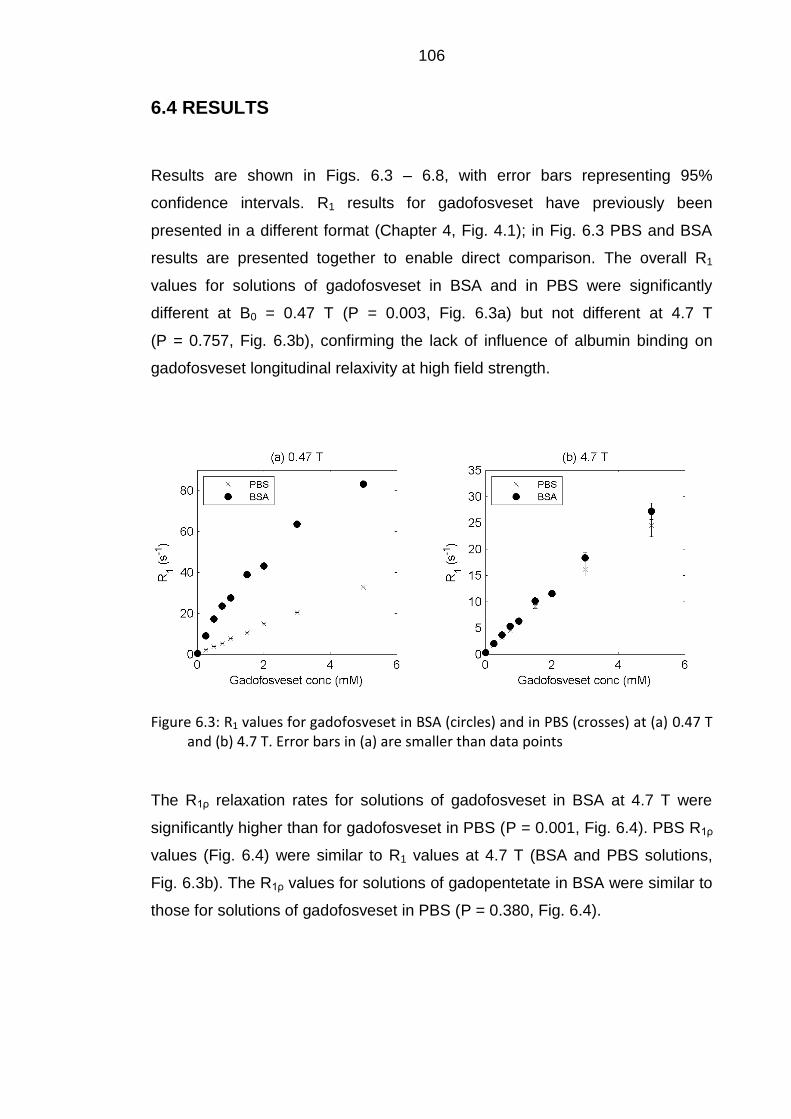
106

6.4 RESULTS

Results are shown in Figs. 6.3 – 6.8, with error bars representing 95%

confidence intervals. R1 results for gadofosveset have previously been

presented in a different format (Chapter 4, Fig. 4.1); in Fig. 6.3 PBS and BSA

results are presented together to enable direct comparison. The overall R1

values for solutions of gadofosveset in BSA and in PBS were significantly

different at B0 = 0.47 T (P = 0.003, Fig. 6.3a) but not different at 4.7 T

(P = 0.757, Fig. 6.3b), confirming the lack of influence of albumin binding on

gadofosveset longitudinal relaxivity at high field strength.

Figure 6.3: R1 values for gadofosveset in BSA (circles) and in PBS (crosses) at (a) 0.47 T and (b) 4.7 T. Error bars in (a) are smaller than data points

The R1ρ relaxation rates for solutions of gadofosveset in BSA at 4.7 T were

significantly higher than for gadofosveset in PBS (P = 0.001, Fig. 6.4). PBS R1ρ

values (Fig. 6.4) were similar to R1 values at 4.7 T (BSA and PBS solutions,

Fig. 6.3b). The R1ρ values for solutions of gadopentetate in BSA were similar to

those for solutions of gadofosveset in PBS (P = 0.380, Fig. 6.4).

107

Figure 6.4: R1ρ values for gadofosveset in BSA (circles) and in PBS (crosses) and gadopentetate in BSA (squares) at B0 = 4.7 T, B1L = 90 μT

R2 values for solutions of gadofosveset in BSA and in PBS at 0.47 T displayed

a similar pattern to R1 values at this field strength, with significantly higher R2

values for the BSA solutions (P = 0.032, Fig. 6.5a). R2 values for equivalent

solutions at 4.7 T were comparable to the R2 values at 0.47 T and the R1ρ

values at 4.7 T, with the BSA R2 values being significantly higher than the PBS

R2 values (P < 0.001, Fig. 6.5b).

Figure 6.5: R2 values for gadofosveset in BSA (circles) and in PBS (crosses) at (a) 0.47 T and (b) 4.7 T. Error bars in (a) are smaller than data points

Measurement of R1, R1ρ and R2 for gadofosveset in mouse plasma at

B0 = 4.7 T and B1L = 90 μT (Fig. 6.6) shows that R1ρ and R2 are similar and

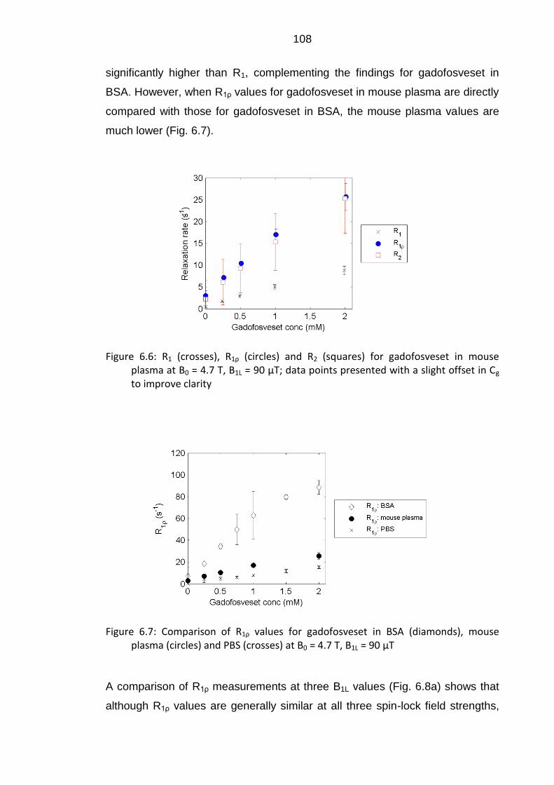
108

significantly higher than R1, complementing the findings for gadofosveset in

BSA. However, when R1ρ values for gadofosveset in mouse plasma are directly

compared with those for gadofosveset in BSA, the mouse plasma values are

much lower (Fig. 6.7).

Figure 6.6: R1 (crosses), R1ρ (circles) and R2 (squares) for gadofosveset in mouse plasma at B0 = 4.7 T, B1L = 90 μT; data points presented with a slight offset in Cg to improve clarity

Figure 6.7: Comparison of R1ρ values for gadofosveset in BSA (diamonds), mouse plasma (circles) and PBS (crosses) at B0 = 4.7 T, B1L = 90 μT

A comparison of R1ρ measurements at three B1L values (Fig. 6.8a) shows that

although R1ρ values are generally similar at all three spin-lock field strengths,

109

the confidence intervals are generally much larger at lower B1L. Image quality is

noticeably poorer at 5 μT when sample images from each of the three spin-lock

fields are visually compared (Fig. 6.8 (b – d)).

(b) TSL = 1.0 ms, B1L = 90 μT

(c) TSL = 1.0 ms, B1L = 25 μT

(d) TSL = 1.0 ms, B1L = 5 μT

Figure 6.8: (a) Plot of calculated R1ρ at three B1L values for gadofosveset in BSA (data points presented with a slight offset in Cg to improve clarity); sample images at TSL = 1.0 ms at (b) B1L = 90 μT, (c) B1L = 25 μT, and (d) B1L = 5 μT

6.5 DISCUSSION

6.5.1 Spin locking

The high albumin-binding affinity of gadofosveset differentiates it from other

clinically approved Gd-based contrast agents. The influence of binding on

gadofosveset R1 is clear at 0.47 T (Fig. 6.3a), but is not observed at 4.7 T

(Fig. 6.3b). Most clinical scanners operate at 3.0 T or lower, where the

longitudinal relaxivity of gadofosveset in the presence of albumin is still higher

110

than other Gd agents (91). However, as clinical field strengths continue to

increase, this advantage of high relaxivity diminishes and an alternative method

for exploiting gadofosveset characteristics would be of benefit. This study

demonstrates the feasibility of a previously unpublished method for combining

the albumin-binding properties of gadofosveset with the macromolecular

sensitivity of spin locking to generate improved contrast modification at high

field strengths. R1ρ values at 4.7 T for BSA solutions containing mostly bound

gadofosveset were found to be significantly greater than R1ρ values for PBS

solutions containing unbound gadofosveset at the same concentration

(Fig. 6.4).

Because of the sensitivity of the SL technique to macromolecules, it is not clear

from these findings alone the extent to which the difference in R1ρ is attributable

to the binding of gadofosveset or the presence of serum albumin

macromolecules. Comparison of R1ρ values for BSA and PBS solutions in the

absence of contrast agent (0 mM) should give an indication of the influence of

the albumin molecules on SL relaxation. However, the lengthy relaxation times

of these blank solutions led to poor model fits to signal intensity data. Instead,

the influence of albumin is better illustrated here by measurements using the

non-binding contrast agent gadopentetate in BSA. A previous study at contrast

agent concentrations ≤ 0.5 mM (91) showed longitudinal relaxivity values at

4.7 T to be higher for gadofosveset in water than for gadopentetate in plasma

(5.5 versus 3.7 mM-1 s-1, respectively). If the SL relaxivity of gadopentetate in

BSA is found to be higher than that of gadofosveset in PBS, this may be

attributable to the BSA solution macromolecules. The R1ρ values for solutions

of gadopentetate in BSA and gadofosveset in PBS (Fig. 6.4), and their

associated relaxivity values, were not significantly different. The similarity of R1ρ

values for gadofosveset in PBS and gadopentetate in BSA together with the

observation of relatively large R1ρ values for gadofosveset in BSA all suggest,

firstly, that the gadolinium has a greater effect on R1ρ than the mere presence

of the macromolecule and, secondly, that it is the binding rather than any non-

specific interactions with the protein that has the largest effect on R1ρ.

111

Further evidence for the influence of binding on R1ρ is provided by the R1ρ

measurements of gadofosveset in mouse plasma. Gadofosveset binds at a

lower fraction in mouse plasma (approximately 67% versus 91% in human

plasma (75)), primarily due to a lower albumin concentration (3.3% in mice (79)

compared to around 4.5% in humans (68)). A comparison of R1ρ for

gadofosveset in mouse plasma and for gadofosveset in BSA at a concentration

equivalent to that found in human serum albumin (Fig. 6.7) clearly shows that

although mouse plasma R1ρ values are higher than those recorded in PBS,

they are still significantly lower than values recorded in BSA, as would be

expected from the differences in bound fraction. This mouse plasma data

shows a potential problem with translating the outcome of pre-clinical studies

with this technique.

Although the SL contrast alteration observed with gadofosveset is not seen to

the same extent with a small Gd-based non-binding contrast agent in an

equivalent macromolecular solution (Fig. 6.4), SL has previously been

successfully utilised in combination with non-binding agents (218, 221, 223,

224). The outcome of this study suggests that additional contrast may be

generated by exploiting the albumin-binding characteristics of an agent such as

gadofosveset, although the reduced extravasation of the bound molecule may

limit the extent of any increases in tissue contrast. Although it is not possible to

use R1 measurements to differentiate signal alteration from bound and free

gadofosveset at high field, due to their equivalent relaxivities (see Chapter 4,

Table 4.2), it may be possible to differentiate bound and free gadofosveset

through spin locking as R1ρ is substantially altered by binding.

It should be noted that for this in vitro study it was not necessary to optimise SL

imaging parameters to take into account potential tissue heating issues

resulting from high SAR. For the majority of measurements a relatively high B1L

value of 90 µT was chosen to give improved image quality. Although R1ρ

increases as B1L decreases, images become increasingly susceptible to

artefacts caused by magnetic field inhomogeneities at very low B1L values

(216). This finding is confirmed by the large error bars at low B1L in Fig. 6.8a

and the prominent image artefacts at 5 µT in Fig. 6.8d, although artefacts at a

112

B1L of 25 µT were less obvious. A range of patient and volunteer studies have

successfully applied spin locking in vivo with a B1L value of 500 Hz (11.7 µT) at

B0 values of 1.5 T (216, 222, 229) and at 3.0 T (230-232). Other methods for

reducing SAR, such as off-resonance spin locking (233), were not explored in

this study.

6.5.2 Transverse relaxation rates

To avoid SAR-related constraints when carrying out in vivo measurements, an

alternative, more practical solution may be to exploit the differences between

bound and free gadofosveset transverse relaxation rates (R2). T2 values are

regularly acquired on clinical scanners, and the effect of gadofosveset is clearly

shown by R2 values in the presence and absence of albumin at 4.7 T

(Fig. 6.5b). For these in vitro solutions, both R2 and R1ρ demonstrate greater

relaxation for bound gadofosveset than R1. Transverse relaxation rates for

gadofosveset will be explored further in Chapter 7.

Although measurement of T2 is more easily achieved in practice than T1ρ, T1ρ is

less influenced by the effect of diffusion from microscopic susceptibility

gradients. As a result several studies, in particular those looking at tumour

response to cytotoxic treatment, have suggested that T1ρ may be a more

responsive early indicator of physiological change than T2 (219, 220). It has

also been suggested that improved (qualitative) tumour boundary definition

may be achieved utilising T1ρ rather than T2 (234). A study of brain images in

healthy volunteers at 1.5 T (235) found that T1ρ-weighted images displayed

improved spatial resolution over T2-weighted images and in vivo T1ρ maps had

a greater dynamic range than equivalent T2 maps, due to the tissue T1ρ signal

only being sensitive to the spin-lock pulse frequency.

6.5.3 Limitations

The scanning parameters at 4.7 T were optimised for physiological contrast

agent concentrations. As a result, model fitting was less precise for the

113

solutions containing the lowest and highest concentrations. The long T1 values

on the 0 mM solutions caused particular problems with model fitting and were

excluded from this analysis. In addition, the PBS R2 values at 4.7 T were based

on a model fit to just three TE points, rather than the six points used for the

BSA solutions, leading to greater imprecision in the calculated PBS R2 values.

For the purpose of this study gadopentetate was assumed to be a non-binding

contrast agent, although there is some evidence to suggest that the chelate

displays a weak tendency for binding to albumin (41). At the comparatively low

serum albumin concentration used here, however, the measured relaxation

rates suggested little influence of albumin binding for gadopentetate and it may

effectively be considered to be non-binding.

6.5.4 Summary

In summary, this study has shown the R1ρ response to gadofosveset in serum

albumin at high fields to be significantly larger than to a conventional small-

molecule Gd-based contrast agent. This suggests that spin locking may be a

viable method for regaining the longitudinal relaxivity lost by gadofosveset at

high fields, and may also provide an opportunity for additional tissue

characterisation through the differentiation of bound and free gadofosveset

molecules. Despite offering potential benefits, implementation of this method in

a SAR-limited clinical setting would require further investigation of optimal SL

parameters prior to assessment in humans. If pre-clinical evaluation of spin

locking with gadofosveset is undertaken, species differences in albumin levels

must also be considered.

Note: A reduced version of this chapter appeared in the October 2012 edition

of Magnetic Resonance in Medicine (1).

114

CHAPTER 7: A GADOFOSVESET-BASED BIOMARKER OF

TISSUE ALBUMIN CONCENTRATION

7.1 BACKGROUND

Albumin is the most abundant protein in human plasma, accounting for half of

all serum proteins (69); its role within the body was discussed in Chapter 3

(section 3.1.2). Albumin is not stored, but continuously synthesized by the liver

and broken down by most organs in the body. The distribution of albumin may

be described by a single intravascular and two extravascular compartments,

one easily mobilised and exchangeable with the intravascular compartment and

the other remote (particularly in the skin, (236)). Around 33% of albumin is

found in the intravascular compartment, with 49% and 18% in the

exchangeable and remote extravascular compartments, respectively (71). The

normal level of serum albumin in plasma is approximately 3.5 – 5.0 g per

100 ml (237), equating to a concentration of approximately 0.52 – 0.74 mM.

Albumin concentrations may be accurately measured in urine or blood

samples, with altered levels caused by changes in rates of synthesis,

catabolism or extravascular leakage. Low levels of albumin have been linked to

critical illness (238) and may be a risk factor for myocardial infarction (239).

The body’s natural transcapillary exchange rate of around 5% of intravascular

albumin per hour (81) may increase in damaged or angiogenic vessels.

Localised increases in extravascular macromolecular content may be

symptomatic of, for example, reperfused myocardial infarction (157) or tumour

angiogenesis (240).

Although albumin concentrations in blood and urine are valuable indicators of

albumin imbalance, they do not fully describe its biodistribution. Direct

measurement of interstitial albumin concentration is not straightforward, with

115

varying results found using invasive techniques such as wick implantation

(241), blister suction (242) or double lumen catheterization (243). It is

suggested that a non-invasive biomarker (244) of localised extravascular

albumin may facilitate quantitative assessment of extravascular leakage. This

technique may have prognostic and/or diagnostic value in assessment of

tumour angiogenesis and response to treatment, as an increase in the leakage

of macromolecules from the vasculature of tumours has been demonstrated

(245). Although conventional small-molecule gadolinium (Gd) contrast agents

are frequently used in MRI to assess microvascular permeability,

macromolecular Gd agents have shown increased sensitivity to malignancy

(159) and response to anti-angiogenic treatment (246). Increased albumin

leakage may also be expected in myocardial infarction (247), where the use of

macromolecular agents may aid assessment of ischaemic microvascular

damage (248).

The general properties of the albumin-binding MRI contrast agent gadofosveset

have been discussed in Chapter 3, with longitudinal relaxivity (r1) assessed in

Chapter 4. In the presence of albumin, gadofosveset r1 is high at low fields but

decreases rapidly as field strength increases (Chapter 4, Fig. 4.4). Conversely,

the transverse relaxivity of the bound molecule is expected to be high at low

field and increase slightly with field strength (89). Results from Chapter 6 show

that, unlike longitudinal relaxation rates (R1, Fig. 6.3), transverse relaxation

rates (R2) are significantly higher for gadofosveset in BSA than in PBS at both

0.47 T and 4.7 T (Fig. 6.5).

The decline in the bound fraction of gadofosveset as contrast agent

concentration increases above a specific value (related to the albumin

concentration, and based on the assumption of a single binding site on the

albumin molecule) suggests that bound fraction may be used as a biomarker

for albumin concentration. Through manipulation of equations presented in

earlier chapters, it is possible to calculate bound and free gadofosveset

concentrations and serum albumin concentration directly from measured R1

and R2 values (with assumed Ka and relaxivity values). This theory holds for

other albumin-binding contrast agents, such as gadoxetate and gadobenate,

116

although these agents have much lower binding affinities (and lower peak

bound fractions). The accuracy of the albumin calculation model is dependent

on accurate R1 and R2 measurements; for agents with low binding affinity,

results may be increasingly susceptible to experimental imprecision in the

measurement of R1 and R2.


This study aims to assess the viability of utilising measured relaxation rates in

solutions with and without gadofosveset to develop a biomarker of albumin

concentration in vitro. The viability of this method is also assessed in vitro using

gadoxetate and gadobenate, and the feasibility of applying the method in a

clinical setting is tested in vivo using gadofosveset-enhanced images from a

small (n = 7) volunteer study. The following objectives were set:

1. Carry out simulation studies to assess the potential influence on albumin

calculation of realistic experimental imprecision in R1 and R2.

2. Measure R1 and R2 at two field strengths for in vitro solutions of

gadofosveset, gadoxetate and gadobenate, along with the non-binding agent

gadopentetate.

3. Calculate bound and free relaxivities based on measured relaxation rates,

and use these results to determine bound fractions and albumin concentrations

for each solution.

4. Use the relaxivity values derived in vitro, along with measured in vivo R1 and

R2 values, to determine gadofosveset and albumin concentrations in left

ventricular blood and myocardial tissue of healthy human volunteers at 3.0 T.

If the method is successful, it may be applied to generate a spatially located

measure of tissue albumin which could be used as an alternative to current

117

invasive techniques. Identification of abnormal extravascular albumin

distribution correlating with increased capillary leakage may have a number of

applications, including early indication of disease progression or treatment

response in tumour angiogenesis, or assessment of reperfused myocardial

infarction.

7.3 THEORY

7.3.1 Bound fraction

Basic theory relating to albumin-binding contrast agents is covered in

Chapter 3; key equations are repeated here with their original numbering. The

overall contrast agent (Cg) and serum albumin (Csa) concentrations equal the

sum of their bound and free components (Eq. 3.3 and 3.4).

[3.3]

[3.4]

Assuming gadofosveset binds at a single site on the albumin molecule,

Cgbound = Csabound; binding affinity (Ka) is then defined by Eq. 3.6.

( ) [3.6]

Bound fraction (fb, Cgbound/Cg) decreases as Cg increases, with the highest fb

occurring when Cg (and therefore Cgbound) is very low. As Cgbound approaches 0,

a first order Taylor expansion of Eq. 3.6 provides a theoretical maximum bound

fraction (fbmax, Eq. 7.1). A step-by-step derivation of this equation is provided in

Appendix C.

118

( ) [7.1]

Assuming gadofosveset, gadoxetate and gadobenate Ka values of 11.0 mM-1 ,

0.255 mM-1 and 0.226 mM-1, respectively, fbmax in human plasma (with an

assumed Csa value of 0.7 mM) at very low Cg would be 0.89 (gadofosveset),

0.15 (gadoxetate) and 0.14 (gadobenate).

Replacing Cgfree in Eq. 3.6 using Eq. 3.3, the quadratic may be solved to give

an expression for Cgbound if total contrast agent concentration, albumin

concentration and binding affinity are known (Eq. 7.2).

√( )

[7.2]

Only the negative form of the quadratic solution is applicable as the positive

form would give a non-zero solution for Cgbound at Cg = 0. Fig. 7.1a shows the

variation of Cgbound with Cg using Eq. 7.2, with Csa = 0.7 mM and Ka = 11.0,

0.255 and 0.226 mM-1 (for gadofosveset, gadoxetate and gadobenate,

respectively). With the assumption of a 1:1 binding ratio of the contrast agent to

albumin, the plot shows that Cgbound approaches a maximum value equivalent to

Csa at high Cg. The variation of bound fraction with Cg (using the same fixed

parameters) is plotted in Fig. 7.1b, with fb approaching fbmax at very low Cg.

119

Figure 7.1: Modelled variation of (a) bound concentration and (b) bound fraction with total gadofosveset concentration, for Csa = 0.7 mM and Ka = 11.0 mM-1

(gadofosveset), 0.255 mM-1 (gadoxetate) and 0.226 mM-1 (gadobenate); note semi log scale on (b)

7.3.2 Measuring albumin binding fraction

As represented in Chapter 4, the contrast-agent induced change in relaxation

rate Ri (ΔRi) for non-binding Gd-based contrast agents, or albumin-binding

agents in the absence of albumin, is conventionally represented by a linear

relationship, defined by the free relaxivity (rifree) (Eq. 4.1).

[4.1]

where i = 1,2.

For an albumin-binding agent composite relaxivities are observed, comprising

contributions from both the bound (ribound) and free molecule, and variations of

Eq. 3.8 (Chapter 3) may be used (Eq. 7.3 and 7.4).

[7.3]

[7.4]

120

Assuming ΔR1 and ΔR2 may be measured and r1bound, r1free, r2bound and r2free are

known, it is possible to rearrange Eqs. 7.3 and 7.4 to give expressions for

bound and free contrast agent concentrations (Eqs. 7.5 and 7.6).

[7.5]

[7.6]

Total contrast agent concentration is then defined by Eq. 7.7.

( ) ( )

[7.7]

Bound, free and overall contrast agent concentrations can therefore be derived

from measurement of ΔR1 and ΔR2.

7.3.3 Measuring albumin concentration

In a second step, contrast agent concentration is related to albumin

concentration by assuming a chemical equilibrium between free and bound

substances. Eq. 3.6 can be rearranged for Csa (Eq. 7.8).

[7.8]

Inserting Eqs. 7.5 and 7.6 into Eq. 7.8 gives an expression for total albumin

concentration (Eq. 7.9).

[7.9]

121

Eq. 7.9 therefore provides a method for deriving albumin concentration through

measurement of ΔR1 and ΔR2, assuming fixed relaxivity and binding

affinity values.

7.3.4 Measuring bound relaxivity

It remains to derive a method for measuring the relaxivity values from in vitro

samples with known contrast agent concentrations. Free relaxivity is derived

using Eq. 4.1, applied to a solution without albumin. An equation for bound

relaxivity is provided in Chapter 3 (Eq. 3.10).

( ) {( ) [( )

]

}

[3.10]

where i = 1,2.

Eq. 3.10 has been represented in a similar form in a number of papers (for

example, (37, 77, 78)). This model describes a gradual transition of binding

fraction, from a maximum at low Cg, where observed relaxivity is dominated by

r1,2bound, towards a minimum at high Cg, where r1,2free has the greater influence.

As the model assumes a single binding site, the shift in emphasis from r1,2bound

to r1,2free occurs at around Cg = Csa.

Accepting that r2bound > r2free and Cgfree > 0, it follows from Eq. 3.3 and Eq. 7.4

that, in all cases:

[7.10]

It should be noted that experimental imprecision in R2 measurement (and R1

measurement, as Cg is calculated using Eq. 7.7) may violate this inequality,

and may lead to calculated values of Csa ≤ 0 mM. For transverse relaxivity,

122

r2bound is much higher than r2free at all B0 values; for longitudinal relaxivity, r1bound

is much higher than r1free at low B0 but both are effectively equivalent at very

high B0 (89). This variation with field strength means that at low B0 any

imprecision in R2 measurement has a much greater influence on calculated Cg

(Eq. 7.7), therefore it is expected that the albumin-calculation model may not be

applicable at low B0 values.

7.4 EXPERIMENTAL METHOD

7.4.1 Simulation

The influence of experimental imprecision in the measurement of ΔR1 and ΔR2

on calculated Csa was assessed through simulation. Estimated 3.0 T relaxivity

values for gadofosveset and gadoxetate were applied to Eq. 3.10 with fixed Ka

values of 11.0 mM-1 (gadofosveset) and 0.255 mM-1 (gadoxetate) to determine

‘true’ ΔR1 and ΔR2 values within the Csa range 0.1 – 1.0 mM and at Cg = 0.1

and 1.0 mM. These ΔR1 and ΔR2 values were then independently adjusted by

± 10% and inserted into Eq. 7.9 in order to determine a calculated Csa. Results

from Chapter 4 suggest that 95% confidence intervals of around ± 10% are

realistic for measurement of relaxation rates.

A further simulated study incorporated a randomly fluctuating variance in both

ΔR1 and ΔR2 (rather than a fixed ± 10%), limited to a Gaussian distribution with

a 5% standard deviation. Csa was calculated for each random variance and the

process repeated 1000 times.

7.4.2 In vitro validation

Model validation was carried out by calculating Csa (using Eq. 7.9) for a range

of in vitro solutions. This requires values of Ka, ΔR1, ΔR2, r2bound, r2free, r1bound

and r1free. ΔR1 and ΔR2 were measured within the study, fixed Ka values of

123

11.0, 0.255 and 0.226 mM-1 for gadofosveset, gadoxetate and gadobenate,

respectively, were assumed, and relaxivity values were derived from the data

(as values for matching experimental conditions could not be found in the

literature).

In vitro solutions of gadofosveset (Vasovist), gadopentetate (Magnevist),

gadoxetate (Primovist) and gadobenate (MultiHance) were prepared in

phosphate-buffered saline (PBS) and bovine serum albumin (BSA) using the

method described in Chapter 4, at concentrations shown in Table 7.1. In total,

28 combinations of gadofosveset and BSA were prepared, along with 12

combinations of contrast agent and BSA for gadoxetate and gadobenate.

Table 7.1: Contrast agent–serum albumin concentration combinations used for in vitro solutions

Contrast agent concentration, Cg

Contrast agent mM % (w/v) (mM)

0.0 - 0, 0.1, 0.2, 0.3, 0.4, 0.5, 0.6, 0.7, 0.8, 0.9, 1.0

0.15 1.0% 0, 0.1, 0.2, 0.3, 0.4

0.3 2.0% 0, 0.1, 0.2, 0.3, 0.4, 0.6, 0.8, 1.0

0.45 3.0% 0, 0.2, 0.3, 0.4, 0.5, 0.6, 0.7, 0.9

0.6 4.0% 0, 0.2, 0.5

0.7 4.7% 0, 0.2, 0.4, 0.6, 0.7, 0.8, 1.0

1.0 6.7% 0,0.6, 1.0

0.3 2.0% 0, 0.1, 0.2, 0.3, 0.4, 0.6, 0.8, 1.0

0.45 3.0% 0, 0.2, 0.3, 0.4, 0.5, 0.6, 0.7, 0.9

0.7 4.7% 0, 0.2, 0.4, 0.6, 0.7, 0.8, 1.0

0.0 - 0, 0.2, 0.5, 0.7, 1.0

0.45 3.0% 0, 0.2, 0.5, 0.7, 1.0

0.7 4.7% 0, 0.2, 0.5, 0.7, 1.0

1.0 6.7% 0, 0.2, 0.5, 0.7, 1.0

0.0 - 0, 0.2, 0.5, 0.7, 1.0

0.45 3.0% 0, 0.2, 0.5, 0.7, 1.0

0.7 4.7% 0, 0.2, 0.5, 0.7, 1.0

1.0 6.7% 0, 0.2, 0.5, 0.7, 1.0

Albumin concentration, Csa

Gadofosveset

Gadopentetate

Gadoxetate

Gadobenate

124

7.4.3 In vitro data acquisition: 3.0 T

Tubes were placed vertically within a head coil (SENSE-Head 8) in a 3.0 T

Philips Achieva TX system at room temperature (approximately 21 °C). R1

values were measured using a spin echo inversion recovery sequence with 10

inversion times (TI = 50, 83, 136, 225, 371, 611, 1009, 1665, 2747, 4925 ms),

TR = 5000 ms, TE = 6.2 ms. R2 values were measured using a multi-echo

sequence with eight echo times (TE = 10, 20, 30, 40, 50, 60, 70, 80 ms),

TR = 1000 ms. Even echoes only were used for model fitting. Additional

parameters common to both R1 and R2 measurement: FOV = 231 x 231 mm;

matrix size = 240 x 240 pixels; single coronal (horizontal) slice; slice

thickness = 10 mm.

7.4.4 In vitro data acquisition: 4.7 T

Tubes were placed vertically in a cylindrical cradle of diameter 60 mm and

inserted into a 63 mm quad coil in a horizontal bore 4.7 T magnet with Bruker

console running ParaVision 5.1 software (Bruker BioSpin MRI GmbH, Ettlingen,

Germany). Solutions were maintained at a temperature of 37 °C with warm air

flow, verified with a fibre optic temperature probe in an adjacent water tube. R1

values were measured using a RARE saturation recovery imaging sequence,

with nine recovery times (57.2, 68.5, 78.5, 88.5, 103.5, 183.5, 283.5, 383.5,

983.5 ms for gadofosveset and gadopentetate; 57.2, 68.5, 78.5, 88.5, 103.5,

183.5, 483.5, 983.5, 2983.5 ms for gadoxetate and gadobenate) and a TE of

11 ms. R2 values were measured using a multi-slice multi-echo (MSME)

sequence, with 20 equally spaced TE values from 11 to 220 ms and a TR of

1000 ms. Additional parameters common to both R1 and R2 measurement:

FOV = 60 x 60 mm; matrix size = 256 x 256 pixels; RARE factor = 2;

averages = 1; centric encoding; single coronal (horizontal) slice; slice

thickness = 1 mm.

125

7.4.5 Relaxation rates

A circular region of interest (ROI) was drawn within each tube and the mean

signal intensity (SI) of each ROI measured using ImageJ software (v1.42q,

Rasband, W.S., ImageJ, U. S. National Institutes of Health, Bethesda,

Maryland, USA, http://imagej.nih.gov/ij/, 1997-2011). SI values at 4.7 T were

adjusted for noise bias using a simple Rician correction (227), based on mean

standard deviations of four background regions in each image. R1 values at

4.7 T and R2 values at 3.0 T and 4.7 T, along with 95% confidence intervals,

were determined from two-parameter nonlinear fits to Eqs. 7.11 and 7.12,

respectively, using MATLAB (v 7.9, MathWorks, Natick, MA). R1 calculation at

3.0 T included an extra term for TR (Eq. 7.13).

( ) [7.11]

[7.12]

[7.13]

where S0 represents the fully recovered SI value and b is a factor accounting for

imprecision in the 180° inversion pulse, applied to each ROI.

Contrast agent-induced changes in relaxation rate (ΔR1,2) were calculated by

subtracting R1,2 values for each non-Gd Csa solution (Cg = 0) from equivalent

Gd-containing Csa solutions (Cg > 0).

7.4.6 Calculating relaxivity and Csa

Once ΔR1 and ΔR2 values were established, Csa calculation was a three-step

process. In the first step, r1free and r2free were calculated by applying the linear

model in Eq. 4.1 to the ΔR1 and ΔR2 values for the contrast agent–PBS

samples (Csa = 0 mM), where no binding was assumed. The second step then

used these free relaxivities and ΔR1 and ΔR2 values to calculate bound

relaxivities. To prevent bias, bound relaxivities were calculated separately for

126

each sample by adopting a leave-one-out approach. For example, for the

gadofosveset Csa = 0.15 mM, Cg = 0.1 mM sample, r1bound and r2bound were

calculated using Eq. 3.10 by applying one-parameter fits to the ΔR1 and ΔR2

values for all the other gadofosveset samples. In this way, a unique set of

relaxivity values were calculated for each sample.

The final step in the process then used the calculated relaxivities and

measured ΔR1 and ΔR2 values for a given sample (for example, for the

Csa = 0.15, Cg = 0.1 mM sample) and applied Eq. 7.9 to determine a calculated

Csa value for that sample. This process was repeated for each sample until an

individual Csa value was calculated for each sample.

In addition, an overall, observed relaxivity (r1obs, r2obs) was calculated for each

set of Csa > 0 mM samples by applying a linear fit to the contrast agent–BSA

ΔR1 and ΔR2 values.

7.4.7 Temperature adjustment

Although measurements at 3.0 T were made at room temperature

(approximately 21 °C), equivalent relaxivity values at body temperature were

also required. To determine a method for adjusting 3.0 T relaxivities at 21 °C to

37 °C equivalents, temperature-related relaxivity values from published studies

were reviewed and supplemented by data acquired at other B0 values as part

of this project.

Relaxivity of the free gadofosveset molecule is expected to decrease as

temperature increases (37). At 3.0 T, a decrease in r1free of around 25% from

room to body temperature has been shown (77); calculated values at 4.7 T in

Chapter 4 (Table 4.2) show a similar decrease. Measurement of gadopentetate

r2 at 1.5 T showed a decrease between room and body temperature of 35%

(93); assuming the free gadofosveset molecule has similar attributes to the

non-binding gadopentetate molecule, this gives an indication of the likely

change in gadofosveset r2free with temperature at 3.0 T.

127

Studies of r1bound at low field demonstrate an opposite temperature

dependence, increasing between room and body temperature (37). However,

this relationship alters as field strength increases (75). Data collected here at a

range of field strengths (Chapter 4, Table 4.2) demonstrate this variation, with

r1bound being 27% higher at 37 °C than at 21 °C at 0.47 T, but 12% lower and

13% lower at 37 °C at 4.7 T and 9.4 T, respectively. It was not possible to find

direct indication of the likely change in r2bound at 3.0 T. However, r2bound (unlike

r1bound) increases with field strength (89), therefore it is suggested that if a

similar increase in r2bound with temperature to r1bound is shown at low field (27%

increase between 21 °C and 37 °C, Table 4.2), a larger increase may be

expected at higher fields.

On the basis of these findings, the following conversions were used to adjust

3.0 T relaxivities from 21 °C to 37 °C: r1free = -25%; r1bound = -10%; r2free = -30%;

r2bound = +40%.

7.4.8 In vivo feasibility assessment: 3.0 T

A total of seven healthy volunteers (five male, mean age 36 ± 10 years, mean

weight 81 ± 15 kg) underwent pre- and post-contrast short-axis cardiac scans

on a 3.0 T Siemens Skyra system at Northwestern Memorial Hospital, Chicago.

The study was approved by the Institutional Review Board (IRB) at

Northwestern University (IRB project number STU00061779, IRB Office,

Northwestern University, Chicago, Illinois), with informed consent obtained from

all participants. IRB approval did not include provision for taking blood samples,

therefore per-volunteer measures of haematocrit and blood albumin were not

available.

Images were acquired as part of a larger study mapping flow patterns in

thoracic aortic aneurisms (TAA) in different progression stages. Myocardial T1

and T2 values with administration of an MR contrast agent were also acquired

to study changes of these parameters associated with inflammatory and

128

connective tissue diseases that are in turn associated with the progression of

TAA. A small timing bolus of 1.0 – 2.0 ml of gadofosveset (Ablavar) was used

to establish arrival time and was followed by a main bolus of 6.2 – 8.8 ml,

giving a total dose of 0.12 ml kg-1 (0.03 mmol kg-1). A modified Look-Locker

inversion recovery (MOLLI) sequence (249) with motion correction (250) (field

of view = 270 x 360 mm, matrix size = 144 x 256 pixels, flip angle = 35°,

TR = 313.45 ms, TE = 1.13 ms, bandwidth/pixel = 975 Hz) was used for T1,

with T1 maps created inline by the system software. This version of the MOLLI

sequence consisted of two inversions, with three images acquired after the first

inversion (initial effective TI of 120 ms, and RR interval added to the other two

acquisitions), and five images acquired after the second inversion (first effective

TI of 200 ms; 200 ms + RR for subsequent acquisitions). Images were acquired

with a specific trigger delay to select for end diastole. MOLLI acquisition was

followed by a T2 mapping sequence using a single-shot T2-prepared steady-

state free precession (SSFP) acquisition with three T2-preparation echo times:

0, 24, and 55 ms (field of view = 337 x 450 mm, matrix size = 144 x192 pixels,

TR = 201.88 ms, TE = 1.07 ms, flip angle = 40°, bandwidth/pixel = 930 Hz). For

all sequences, 8 mm slices were acquired at cardiac short axis base, mid and

apex locations. Post-contrast images were acquired at up to three time points

for each volunteer, with T2 image acquisition occurring 1 – 2 min after T1

acquisition (Table 7.2). The mid-point between T1 and T2 image acquisitions

was used as the post-contrast reference time.

Table 7.2: Main bolus and image acquisition times for volunteers (time from first administration of contrast agent (timing bolus), MM:SS)

Main

Volunteer bolus T1 [1] T2 [1] T1 [2] T2 [2] T1 [3] T2 [3]

#1 07:08 14:31 16:47 – – – –

#2 03:52 08:57 11:19 38:34 39:35 54:06 55:53

#3 02:35 07:10 08:10 29:12 30:15 – –

#4 04:15 29:17 31:44 – – – –

#5 08:24 41:43 43:25 – – – –

#6 03:24 23:45 25:02 28:09 29:29 39:23 40:38

#7 03:06 05:34 07:21 18:34 20:16 27:02 28:36

Measurement

129

ROIs were drawn within the left ventricle and within the myocardium on each

pre- and post-contrast T1 and T2 map at the middle of the short axis view, and

median and standard deviation values derived using MATLAB. Relaxation

times were converted to relaxation rates and Eq. 7.7 and 7.9 used to determine

gadofosveset and albumin concentrations, respectively. A Ka value of

11.0 mM-1 was assumed and the temperature-adjusted 3.0 T in vitro bound and

free relaxivities used. For albumin calculation each ROI is considered as a

single well-mixed compartment, which is a valid assumption for the left

ventricle, where gadofosveset is entirely intravascular, but is a simplification of

conditions in the myocardium, where ΔR1 and ΔR2 are influenced by

gadofosveset in vascular and extravascular spaces.

7.5 RESULTS

7.5.1 Simulation

Simulated data are shown in Fig. 7.2 and 7.3. The influence on calculated Csa

of a ± 10% variance in ΔR1 or ΔR2 is illustrated by a plot of percentage

difference between calculated and actual Csa for gadofosveset and gadoxetate,

at contrast agent concentrations of 0.1 mM and 1.0 mM (Fig. 7.2). A boxplot of

percentage error in calculated Csa is shown at a gadofosveset concentration of

0.5 mM, with a Gaussian distribution on ΔR1 and ΔR2 variability (Fig. 7.3).

130

Figure 7.2: Simulated effect of error in measured relaxation rate (± 10%) on calculated Csa at Cg = 0.1 mM (left) and 1.0 mM (right) for gadofosveset (top) and gadoxetate (bottom) using representative relaxivity values

131

(a)

(b)

Figure 7.3: (a) Simulated spread of error in calculated Csa for gadofosveset when applying a 5% standard deviation on ΔR1,2 variability using a Gaussian distribution (1000 repetitions; Cg = 0.5 mM, Ka = 11.0 mM-1, representative relaxivity values). Red lines represent median value, box limits are 25th and 75th percentiles, whiskers cover 99.3% of data points and red ‘+’ signs are outliers beyond this range; (b) as (a), with reduced vertical scale to highlight detail

7.5.2 In vitro data at 3.0 T and 4.7 T

Mean individual gadofosveset, gadoxetate and gadobenate relaxivity values

measured at 3.0 T and 4.7 T for the range of Csa – Cg combinations are given

in Table 7.3; standard deviations in brackets indicate the variance in calculated

relaxivity. Calculated 3.0 T relaxivity values were acquired at approximately

21 °C and the values adjusted to 37 °C using the method described in

section 7.4.7.

132

Table 7.3: Calculated relaxivity values and standard deviations (mM-1 s-1)

* Temperature adjustment for 3.0 T data as described in methods (section 7.4.7)

Figs. 7.4 and 7.5 show gadofosveset, gadoxetate and gadobenate model fits

(Eq. 3.10) plotted against actual ΔR1 and ΔR2 data points for three

(gadofosveset) or two (gadoxetate and gadobenate) Csa values at 3.0 T

(Fig. 7.4) and 4.7 T (Fig. 7.5), using the mean individual relaxivities in

Table 7.3, along with a linear fit to the gadopentetate data.

The bound relaxivity values in Table 7.3 were based on a range of Csa values.

Observed relaxivity values (r1obs and r2obs) were not included in this table as it

was expected there may be an underlying relationship between observed

relaxivity and Csa. Fig. 7.6 shows the variation in observed relaxivity with Csa at

3.0 T and 4.7 T, based on a linear fit to ΔR1 and ΔR2 data points for the BSA

solutions.

Fig. 7.7 shows calculated bound fractions derived from ΔR1 and ΔR2

measurements (Eqs. 7.5 and 7.7) for gadofosveset, gadoxetate and

gadobenate, at all albumin concentrations and at 3.0 T and 4.7 T, along with

theoretical bound fractions for each albumin concentration (Eq. 7.2).

In Fig. 7.8 calculated Csa values (using Eq. 7.9) are compared to actual values

for each solution using individually derived relaxivity values at 3.0 T and 4.7 T.

Two data points for gadofosveset at 4.7 T, one point for gadobenate at 3.0 T

and two points for gadobenate at 4.7 T are missing from these plots as they

Gadofo

sveset

Gadoxeta

te

Gadobenate

Gadofo

sveset

Gadoxeta

te

Gadobenate

Gadofo

sveset

Gadoxeta

te

Gadobenate

r1bound 12.2 (0.3) 11.6 (0.6) 13.9 (1.5) -10% 11.0 10.4 12.5 6.5 (0.0) 5.5 (1.4) 8.6 (4.6)

r1free 8.1 (0.3) 7.4 (0.2) 5.7 (0.1) -25% 6.0 5.6 4.3 4.5 (0.1) 5.2 (0.3) 3.6 (0.1)

r2bound 43.8 (1.0) 28.4 (2.1) 32.9 (2.8) +40% 61.3 39.7 46.1 60 (1.4) 45.8 (2.4) 54.4 (5.4)

r2free 9.7 (0.2) 8.7 (0.2) 7.6 (1.1) -30% 6.8 6.1 5.3 10.7 (1.7) 6.4 (0.1) 4.4 (0.4)

3.0 T, 21 °C 4.7 T, 37 °C3.0 T, adjusted to 37 °C

Tem

pera

ture

adju

stm

ent

*

133

were outside the range shown (calculated Csa more than double actual Csa).

Four gadofosveset data points at 4.7 T violated the inequality described in

Eq. 7.10 and gave negative values of calculated Csa, and were therefore also

excluded. For gadofosveset, the model-derived Csa values correlate with actual

Csa at a statistically significant level at both field strengths (Pearson correlation

coefficients of 0.95 and 0.88 for 3.0 T and 4.7 T, respectively). If the two points

not shown in Fig 7.8b for gadofosveset are excluded from the calculation, the

Pearson correlation at 4.7 T increases to 0.95. For gadoxetate, a significant

correlation between actual and calculated Csa is seen at 4.7 T, but not at 3.0 T

(Pearson correlations of 0.89 and 0.33, respectively). For gadobenate, no

correlation was seen between actual and calculated Csa at either field (-0.13 at

3.0 T and -0.03 at 4.7 T); even excluding the two data points not shown in

Fig. 7.8f, the correlation is still not significant (0.37).

134

Figure 7.4: ΔR1 (left column) and ΔR2 (right column) values at 3.0 T (at room temperature) for gadofosveset (circles) and gadopentetate (squares) at Csa = 0.3, 0.45 and 0.7 mM, and gadoxetate (diamonds) and gadobenate (stars) at Csa = 0.45 and 0.7 mM; error bars indicate 95% confidence intervals. Gadofosveset, gadoxetate and gadobenate model fits (Eq. 3.10, solid, dotted and dot-dash lines, respectively) are represented using mean relaxivity values (Table 7.3); a linear fit is applied to gadopentetate data (Eq. 4.1, dashed line)

135

Figure 7.5: ΔR1 (left column) and ΔR2 (right column) values at 4.7 T (at body temperature) for gadofosveset (circles) and gadopentetate (squares) at Csa = 0.3, 0.45 and 0.7 mM, and gadoxetate (diamonds) and gadobenate (stars) at Csa = 0.45 and 0.7 mM; error bars indicate 95% confidence intervals. Gadofosveset, gadoxetate and gadobenate model fits (Eq. 3.10, solid, dotted and dot-dash lines, respectively) are represented using mean relaxivity values (Table 7.3); a linear fit is applied to gadopentetate data (Eq. 4.1, dashed line)

136

Figure 7.6: Variation of observed relaxivity (r1obs, left column; r2obs, right column) with Csa at 3.0 T (circles) and 4.7 T (squares), based on linear fit to BSA ΔR1 and ΔR2 values

137

Figure 7.7: Calculated bound fraction (Cgbound/Cg) based on measured data using Eq. 7.5 and 7.7 at Csa = 0.15 (circles), 0.3 (diamonds), 0.45 (stars), 0.7 (squares) and 1.0 mM (crosses); lines represent theoretical bound fraction using Eq. 7.2 and literature binding affinity values quoted previously at Csa = 0.15 (black solid line), 0.3 (dot-dash line), 0.45 (dotted line), 0.7 (dashed line) and 1.0 mM (grey solid line)

138

Figure 7.8: Spread of calculated Csa values (represented as a percentage difference to actual Csa) using Eq. 7.9; two data points in (b) are beyond plot scale (calculated Csa = 0.55 mM, actual Csa = 0.15 mM; calculated Csa = 0.63 mM, actual Csa = 0.3 mM); one data point in (e) is beyond plot scale (calculated Csa = 2.82 mM, actual Csa = 0.45 mM); two data points in (f) are beyond plot scale (calculated Csa = 2.41 mM, actual Csa = 0.45 mM; calculated Csa = 2.53 mM, actual Csa = 0.7 mM)

139

7.5.3 Volunteer data at 3.0 T

Figure 7.9: Example of (a) pre-contrast and (b) post-contrast T1 maps (T1 values calculated separately for each pixel and assigned a greyscale value) for a single volunteer, with left ventricle (LV) surrounded by myocardium in centre of image

Examples of pre- and post-contrast T1 maps for one volunteer are shown in

Fig. 7.9. Pre-contrast T1 values in the left ventricle and myocardium were in the

range 1493 – 1818 ms and 1099 – 1124 ms, respectively. Pre-contrast T2

values in the left ventricle and myocardium were in the range 117 – 158 ms and

43 – 47 ms, respectively.

Calculated gadofosveset and albumin concentrations in the left ventricle and

myocardium are shown in Fig. 7.10, with data for all seven volunteers plotted

against time from first bolus administration. The models for calculating

gadofosveset (Eq. 7.7) and albumin (Eq. 7.9) concentrations used the

temperature-adjusted 3.0 T relaxivity values shown in Table 7.3.

140

Figure 7.10: Calculated (a) gadofosveset and (b) albumin concentrations in left ventricle (filled symbols) and myocardium (open symbols) in healthy volunteers at 3.0 T. Each symbol shape represents a different volunteer; values are plotted against time from first administration of contrast agent (to mid-point between T1 and T2 image acquisition times)

7.6 DISCUSSION

Increased capillary leakage is symptomatic of a range of pathologies and

healthy processes, resulting in rapid wash-in and wash-out of small molecule

contrast agents and an increased transfer of macromolecules, including

intravascular albumin, to the interstitial space. In vivo measurement of

extravascular albumin content is not straightforward, although a range of

invasive techniques are currently available. This study has explored the

possibility of utilising albumin-binding Gd-based contrast agents to generate a

novel and location-specific non-invasive method for measuring levels of

albumin at moderate to high magnetic field strengths. The albumin-calculation

model was assessed in vitro with agents binding in low and high fraction, and in

vivo with the high-binding agent gadofosveset. Pre- and post-contrast R1 and

R2 measurements are regularly carried out in MRI; the models presented here

combine these changes in relaxation rate with calculated relaxivity values and a

literature binding affinity value to produce a basic measure of tissue albumin

concentration.

141

7.6.1 Simulation

At low gadofosveset Cg (Fig. 7.2a), a +10% inaccuracy in ΔR1 or a -10%

inaccuracy in ΔR2 leads to an underestimation of Csa; a -10% inaccuracy in ΔR1

or a +10% inaccuracy in ΔR2 causes the model to behave erratically. This is

due to the denominator in the right-hand term of Eq. 7.9 (r1bound.ΔR2 –

r2bound.ΔR1) approaching zero at a certain combination of shifted relaxation

rates. Results from Chapter 4 suggest that an imprecision in ΔR1 or ΔR2 of 10%

is not unfeasible, therefore it is important that relaxation rates are measured as

accurately as possible, particularly where low gadofosveset concentrations are

expected. At high gadofosveset Cg (Fig. 7.2b), the model performs much more

consistently at intermediate Csa values (0.2 – 0.8 mM): a +10% inaccuracy in

ΔR1 or a -10% inaccuracy in ΔR2 leads to a slight underestimation of Csa; a

-10% inaccuracy in ΔR1 or a +10% inaccuracy in ΔR2 leads to a slight

overestimation of Csa. However, the model becomes increasingly inaccurate at

very high or very low Csa values.

For gadoxetate, an underestimation of Csa results from a +10% inaccuracy in

ΔR1 or a -10% inaccuracy in ΔR2; an overestimation of Csa is caused by a -10%

inaccuracy in ΔR1 or a +10% inaccuracy in ΔR2. The pattern is very similar at

both Cg = 0.1 mM (Fig. 7.2c) and Cg = 1.0 mM (Fig. 7.2d), and shows that

calculated Csa values using gadoxetate are more susceptible to inaccuracies in

ΔR1 and ΔR2 at higher Cg values than gadofosveset. These simulations were

not carried out for gadobenate, but the patterns would be expected to be very

similar to those of gadoxetate.

Although these simulations at the extreme limits of the expected range of

imprecision in ΔR1 and ΔR2 are useful to assess model robustness, a more

realistic simulation would incorporate a Gaussian distribution within this range

of imprecision. Applying such a distribution to a randomly varying error in ΔR1

or ΔR2 for gadofosveset at a concentration of 0.5 mM (Fig. 7.3), it can be seen

that the majority of calculated Csa values have an error much less than 50%.

142

Although the median value is accurate at lower Csa values, the model begins to

underestimate Csa at high Csa values.

7.6.2 In vitro model validation

Gadofosveset relaxivity

Calculated r1 and r2 relaxivity values at both 3.0 T and 4.7 T are in general

agreement with previously published values (91). Using mean calculated

relaxivity values, the model represents a good fit to gadofosveset ΔR1 and ΔR2

data points at all Csa values (Figs. 7.4 and 7.5), suggesting that the assumption

of a single binding site on the albumin molecule is adequate at these

concentrations. The primary binding site is known to provide the greatest

contribution to relaxivity (68), and it is unlikely that Cg levels would be

sufficiently high in vivo during the post-bolus phase to necessitate inclusion of

additional binding sites in this model (78). Although a literature Ka value of

11.0 mM-1 was assumed for these calculations, a plot of Ka at half and double

this value was previously shown to make very little difference to a model fit of

similar data (Chapter 4, Fig. 4.7). It should be noted that in vitro data at 3.0 T

were acquired at room temperature (21 °C). An increase from room to body

temperature reduces the relaxivity of the free gadofosveset molecule slightly;

the relationship between the relaxivity of the bound gadofosveset molecule and

temperature is additionally influenced by field strength, and will differ for r1bound

and r2bound. An attempt was made to adjust room temperature 3.0 T relaxivities

to their body temperature equivalents (Table 7.3), and the resulting values are

similar to those published elsewhere (91). r2obs shows a clear increase with

increasing albumin concentrations at both field strengths (Fig. 7.6b), but this

relationship is less clear for r1obs (Fig. 7.6a).

The longitudinal relaxivity values presented here for gadofosveset differ slightly

from those calculated in Chapter 4. r1free estimates are 7% and 12% lower at

3.0 T and 4.7 T, respectively, in this chapter than estimated in Chapter 4.

However, r1free values in Chapter 4 were based on 8 gadofosveset

143

concentrations in the range 0.25 – 5.0 mM (with four Cg values ≤ 1.0 mM); the

r1free values in this chapter were based on 10 Cg values in the range

0.1 – 1.0 mM. It is possible that some nonlinearity at very high Cg was

introduced in the Chapter 4 data that may have skewed the results slightly.

r1bound values are 2% higher and 12% lower at 3.0 T and 4.7 T, respectively, in

this chapter than in Chapter 4. The r1bound values in Chapter 4 were calculated

based on solutions of gadofosveset at concentrations up to 0.75 mM at a single

fixed serum albumin concentration (Csa = 0.67 mM), whereas the r1bound values

in this chapter are based on a range of Cg concentrations up to 1 mM at five

Csa values between 0.15 mM and 1.0 mM. It is possible that the larger number

of data points used for model fitting in this chapter (28 points, compared to just

8 in Chapter 4), along with a greater range of albumin concentrations, make the

calculated values in this chapter more precise.

Gadoxetate and gadobenate relaxivity

Free relaxivity values for gadoxetate and gadobenate at 3.0 T and 4.7 T are

similar to those published elsewhere (91). It is difficult to find published

relaxivity values for the bound molecule at these field strengths, so the

calculated values could not be directly verified. However, observed relaxivities

at Csa = 0.7 mM (Fig. 7.6c to 7.6f), based on a linear fit to ΔR1 and ΔR2 values

at all Cg values, are comparable with those published elsewhere (91).

r1free values for gadoxetate and gadobenate are identical in this chapter to

those values given in Chapter 4, as the same solution combinations were used.

At 3.0 T, there was very little difference between r1bound values in Chapter 4 and

those given in this chapter. However, at 4.7 T, r1bound values were 20%

(gadoxetate) and 54% (gadobenate) higher in this chapter than in Chapter 4.

Although these differences may appear large, they are not statistically

significant as the 95% confidence intervals overlap. The relatively large

confidence intervals suggest it is more difficult to accurately determine bound

relaxivity values for these agents than for gadofosveset.

144

As may be expected by their relative binding affinities, ΔR1 and ΔR2 values

plotted in Fig. 7.4 and 7.5 are higher for gadoxetate and gadobenate than those

for gadopentetate but lower than those for gadofosveset. As with gadofosveset,

ΔR1 values decrease with field strength; however, unlike gadofosveset, where

ΔR2 values increase between 3.0 T and 4.7 T, the ΔR2 values for both

gadoxetate and gadobenate change very little with field strength.

Bound fraction calculations

Calculated bound fractions for gadofosveset are in good general agreement

with theoretical expected values at 3.0 T (Fig. 7.7a). At 4.7 T (Fig. 7.7b), a

consistent pattern still generally holds, although the value at Csa = 0.15 mM,

Cg = 0.1 mM is higher than expected. For gadoxetate at 3.0 T (Fig. 7.7c),

calculated bound fractions at Csa = 1.0 mM do not behave as expected

(increasing, instead of decreasing, with Cg), but bound fractions at other Csa

values are closer to their theoretical equivalents. For gadoxetate at 4.7 T

(Fig. 7.7d), the bound fraction at Cg = 0.2 mM, Csa = 1.0 mM is higher than

expected, but all other values are close to their expected values. For

gadobenate at both fields (Fig. 7.7e and 7.7f), the bound fractions at the lowest

Cg appear to be too high. This pattern of high calculated bound fraction at low

Cg may be the result of the relative uncertainty in measured Ri0 (relaxation

rates at Cg = 0 mM) having a greater influence on the ΔRi values at low Cg.

A study which derived bound fractions from relaxation rate measurements in

rabbits (78) found bound fractions at 300 s post-bolus of 0.77 and 0.18 for

gadofosveset and gadobenate, respectively (at Cg values of approximately

0.4 mM). Assuming a plasma albumin concentration of 3.9% (approximately

0.6 mM) in rabbits (79), the points plotted in Fig. 7.7 which are closest to these

Cg and Csa values correlate reasonably well.

145

Albumin calculations

If negative calculated Csa values resulting from measurement imprecision are

excluded, a comparison of the remaining calculated and actual Csa values for

gadofosveset (Fig. 7.8a and 7.6b) shows a correlation at a statistically

significant level at both field strengths. Two further data points at 4.7 T were

beyond the chosen scale in Fig. 7.8b, possibly as a result of imprecision in ΔR1

and ΔR2 measurement; if these points are also excluded, the correlation at

4.7 T is strengthened.

For gadoxetate, a significant correlation between actual and calculated Csa is

seen at 4.7 T (Fig. 7.8d), but not at 3.0 T (Fig. 7.8c). For gadobenate, no

correlation was seen between actual and calculated Csa at either field (Fig. 7.8e

and 7.8f); the correlation improves if the two data points not shown in Fig. 7.8f

are excluded, but not to a statistically significant level.

These results highlight the potential difficulty in applying the albumin-calculation

model to agents such as gadoxetate or gadobenate, which bind to albumin at a

relatively low fraction. Although the overall performance of gadofosveset in

calculating Csa is better, there are still data points where the model is

inaccurate or fails altogether (producing negative Csa estimates). Simulated

errors in calculated Csa (Figs. 7.2 and 7.3) suggest the model is susceptible to

imprecision in measured relaxation rates.

Although all three albumin-binding contrast agents were assessed at the same

contrast agent concentrations, gadobenate is used at a higher standard clinical

dose (0.1 mmol kg-1) compared to gadofosveset (0.03 mmol kg-1) or gadoxetate

(0.025 mmol kg-1) (Table 2.1 in Chapter 2). This higher gadobenate dose gives

in vivo concentrations 3 – 4 times those of gadofosveset or gadoxetate, but as

can be seen from Fig 7.1b bound fraction would only be slightly lower at these

higher concentrations. As the albumin-calculation model was assessed here

across a range of albumin and contrast agent concentrations, the results are

still expected to be relevant.

146

The albumin calculation model presented here is expected to work well for

gadofosveset at higher B0 values (3.0 T and above), where there is a large

difference between r2bound and r2free but a small difference between r1bound and

r1free. At low fields, r1bound is close to r2bound and the difference between ΔR1 and

ΔR2 is small. In this case, the precision of the model input parameters would be

insufficient to overcome the sensitivity of the model to the variability in those

parameters. At very high B0, r1bound and r1free values for gadofosveset may be

considered equivalent and the model may be simplified to incorporate a linear

relationship between ΔR1 and Cg. The Cg calculation described in Eq. 7.7 may

then be represented as Cg = ΔR1 / r1.

An underlying correlation between relaxivity and protein content has been

shown in previous studies for Gd-based contrast agents not conventionally

described as albumin binding (41, 251). In vitro gadopentetate ΔR2 data points

are well represented here by a linear fit (Figs. 7.4 and 7.5), suggesting no

observable influence of weak binding on contrast agent relaxivity at the albumin

levels used in this study. Without separate bound and free transverse

relaxivities, gadopentetate provides no means of estimating Csa through

application of the model presented here. The high binding affinity of

gadofosveset makes it a much more sensitive biomarker of albumin.

7.6.3 In vivo feasibility

Gadofosveset-enhanced cardiovascular imaging is an area of active research

(99, 100, 102, 106, 252), and likely to remain so in North America where the

agent is available under the trade name Ablavar. One potential clinical

application of the technique for calculating albumin concentration relates to

myocardial infarction, therefore a feasibility assessment utilising human cardiac

images was considered relevant. Cardiac imaging has the advantage of

enabling direct comparison of calculated albumin values from blood in the left

ventricle and from highly perfused myocardial tissue. However, before the

147

model can be assessed, motion correction and other technical challenges must

be overcome.

Pre-contrast T1 and T2 values obtained here correlate well with literature values

in blood (253, 254) and in the myocardium (253, 255, 256). Combining data

from seven volunteers with images acquired at a range of time points gave

remarkably consistent values of the two model input variables ΔR1 and ΔR2,

and supported calculation of appropriate Cg values in both the left ventricle and

the myocardium (Fig. 7.10a). As expected, gadofosveset concentration peaks

at the earliest time points post-bolus and decreases towards an equilibrium

value, although this was not a dynamic acquisition therefore the temporal

resolution is such that the bolus peak is not fully described. In the left ventricle,

a maximum value of 0.48 mM is calculated at the earliest time points (6 – 8 min

post-bolus), with a later calculated Cg of 0.24 mM (at 55 min post-bolus). Lower

peak and equilibrium gadofosveset concentrations are observed in the

myocardium (0.18 mM and 0.1 mM, respectively).

At a dose of 0.03 mmol kg-1, the average blood concentration of gadofosveset

for an 81 kg adult with a total blood volume of 6.4 L would be 0.4 mM; allowing

for some extravasation and excretion, the gadofosveset values calculated here

in the left ventricle appear reasonable. For a small molecule agent such as

gadopentetate, approximately 50% may diffuse to the extravascular space from

the blood on the first pass through the capillary bed (257). Although, as a ‘blood

pool’ agent, gadofosveset may be expected to remain predominantly within the

intravascular space, at high concentrations (immediately after bolus injection,

for example) the bound fraction will be low and the extravasation rate may be

similar to that of a conventional agent (258). A study in rabbits showed that

61% of injected gadofosveset was still in the blood at 1 minute post-injection

(78). Certainly, a reduction in Cg between the left ventricle and myocardium is

expected, as noted in the relative values here.

Unlike gadofosveset, albumin concentration is expected to remain consistent

within an individual for the image acquisition duration. Although there is some

within-subject variability (Fig. 7.10b), this variability may be representative of an

148

imprecision in the data acquisition and does not correlate with time post-bolus.

The mean calculated albumin concentration in the left ventricle of the seven

volunteers was 0.14 mM (range 0.10 – 0.18 mM); in the myocardium the mean

calculated Csa was 0.03 mM (range 0.00 – 0.07 mM).

A reference measure of albumin concentration was not available for

comparison. Serum albumin levels in plasma (Csa_plasma) are expected to be

approximately 3.5 – 5.0 g dl-1 (0.52 – 0.74 mM) (237). Assuming a haematocrit

(Hct) of 0.42, this equates to albumin levels in whole blood of 0.30 – 0.43 mM

(where blood concentration = Csa_plasma.(1 – Hct)). Previous studies quote

interstitial fluid albumin concentrations (Csa_interstitial) of 0.2 – 0.4 mM (83, 241,

242). However, the myocardium ROI contains intravascular, extravascular

extracellular and intracellular spaces. Neglecting the intracellular space, as

gadofosveset cannot directly access it, and assuming an extracellular volume

fraction (EVF) of 0.25 (259), a myocardial blood volume (MBV) of 8% (260) and

a haematocrit in capillaries (Hctcap) of 0.25, tissue albumin (Csa_tissue,

measurable using gadofosveset) may be expected to be in the range 0.07 –

0.11 mM (where Csa_tissue = MBV.(Csa_plasma.(1 – Hctcap)) + Csa_interstitial.(EVF –

MBV)). This range of expected values assumes that all blood vessels in the

myocardium are capillaries; in reality, a proportion would be larger than

capillaries and would therefore have a higher Hct, leading to a slightly lower

range of expected Csa_tissue values.

Calculated Csa values were lower than might be expected in healthy volunteers.

This underestimation may be partly attributable to the relative timings of the T1

and T2 measurements used as the basis for calculating Csa. Images used for T1

and T2 measurement were taken at different time points post-bolus, with the

images for T2 measurement acquired 1 – 2 minutes after the images for T1

measurement (Table 7.2). This time difference is unlikely to be an issue at the

later time points (within the equilibrium phase). However, at earlier time points,

where the concentration of gadofosveset is initially high and then drops rapidly,

ΔR1 values at the T1 time point are higher than they would be at the equivalent

T2 time point. The model is sensitive to the ratio of ΔR2 to ΔR1; if ΔR1 is

artificially high in relation to ΔR2, the resulting calculated Csa will be lower. This

149

may account for an element of model underestimation in vivo, particularly at the

earlier time points. Also, the gadofosveset dose was administered in the form of

a small timing bolus followed 2 – 8 minutes later by the main bolus. Again, this

is unlikely to have an effect at equilibrium, but could influence calculations at

the earliest time points.

Another consideration is whether the relaxivities used in Csa calculation,

derived in vitro, were directly applicable in vivo. These relaxivities were based

on values determined at room temperature and converted to body temperature;

it is possible that the temperature conversion factor was slightly inaccurate. In

addition, bovine serum albumin was used in vitro; although bovine serum

albumin is structurally similar to human serum albumin, and BSA is often used

as a surrogate for HSA in laboratory studies (for example, (261)), the molecules

may display slightly different binding properties (165). There is also some

evidence to suggest that relaxivities derived in vitro for a non-binding Gd agent

may be higher than equivalent measurements in vivo (262), which may have

implications for the free relaxivity measurements used in this study.

It should also be noted that the bound gadofosveset fraction will be at its

maximum in the left ventricle at equilibrium, where Csa > Cg. The model is less

sensitive in this scenario, as confirmed by the observed underestimation of Csa

at higher albumin concentrations in vitro at 3.0 T (Fig. 7.8a). This feature is also

noted in the median Csa values from the simulated data (Fig. 7.3b). Although

calculations in the left ventricle were carried out in this study, the method may

not be appropriate or necessary here as albumin levels in blood can be readily

measured from blood samples. The primary utility of the method may be in

providing measurement of albumin concentration in tissue, where Cg is lower

and Csa is conventionally difficult to acquire.

A previous study using the contrast agent gadobenate (152) suggested that

renal protein leakage could be identified by analysing tubular flow differences

following injection of two contrast agents, one binding and one non-binding.

Attempts have also been made to map protein levels by utilising the distinct

field dependency of the bound and free gadofosveset molecule (termed delta

150

relaxation enhanced MR, DREMR) (263, 264), although this approach requires

the use of additional hardware to modulate B0. The advantage of the method

described in this study over either of these approaches is that it only requires a

single contrast agent injection and may be readily derived from routinely

acquired R1 and R2 measurements using conventional equipment.

It should be noted that a single MRI voxel on the cardiac T1 maps represents a

volume of tissue 1.9 x 1.4 x 8.0 mm, and on the T2 maps represents a volume

of 2.3 x 2.3 x 8.0 mm. Each myocardial voxel will contain a combination of

interstitial, intravascular and intracellular space, therefore it is difficult to use

this method to isolate and measure interstitial albumin. In reality, the

measurement of albumin will relate to tissue levels, and the interstitial

proportion will depend on the density of vessels and cells within this voxel.

7.6.4 Summary

In summary, the albumin calculation model presented here demonstrates the

feasibility of determining in vitro serum albumin concentration using pre- and

post-gadofosveset measurements of R1 and R2 at high B0 values. The method

was successfully validated using in vitro samples at 3.0 T and 4.7 T. Extending

the methodology to other albumin-binding agents, gadoxetate and gadobenate,

was less successful, due to the low binding fraction of these agents. It was not

possible to implement the method using the non-binding agent gadopentetate.

Feasibility assessment in a small number of human volunteers was performed

using gadofosveset, and consistent ΔR1, ΔR2 and Cg values were determined.

Underestimation of Csa may be the result of several contributing factors,

including the timing of the image acquisitions and translation of in vitro

relaxivities. Due to the withdrawal of gadofosveset from the European market, it

was not possible to complete additional in vivo experiments. However, further

in vivo assessment is suggested, to include: simultaneous T1 and T2

measurement; additionally acquiring images between the timing bolus and the

151

main bolus; and blood sampling to establish Hct and reference blood albumin

levels.

This novel approach may enable non-invasive assessment of extravascular

leakage of albumin, utilising parameters acquired during routine imaging, in

regions where implementation of invasive techniques for measurement of

interstitial albumin is conventionally challenging. A range of potential clinical

applications are envisaged, including assessment of myocardial infarction,

tumour angiogenesis and response to treatment.

152

CHAPTER 8: SUMMARY AND CONCLUSIONS

8.1 SUMMARY

The albumin-binding affinity of gadofosveset makes this molecule unique

amongst the gadolinium-based clinically approved MRI contrast agents.

Binding prolongs its intravascular retention and increases the relaxivity of the

agent, primarily through reduction of the rotational correlation time. However,

the fraction of gadofosveset that binds varies with concentration and the

relaxivities of the bound and free molecules display differential responses to

variations in field strength and temperature.

Although originally intended as an assessment of the in vivo use of

gadofosveset for dynamic contrast-enhanced MRI studies, the lack of

availability of gadofosveset due to its withdrawal from the European market

(shortly after the project commenced) limited the extent to which in vivo studies

could be carried out. As a result, the aims of the project were adjusted to

incorporate further in vitro characterisation of gadofosveset and other albumin-

binding agents, along with the development of a technique that would enable

accurate measurement of a vascular input function which may be of value in

future tracer kinetic studies.

The first aim of this study, therefore, was to address gaps in the current

gadofosveset literature, by determining the relaxivity of the bound and free

molecule across a range of field strengths, and at two temperatures. In

addition, the study addressed the issue of binding sites, by comparing models

incorporating one, two and three bound molecules at a fixed albumin

concentration, and assessed the general influence of binding by measuring

relaxation rates and bound fractions at a range of contrast agent and serum

albumin concentrations, and for gadofosveset in mouse plasma.

153

The second aim of the study was to assess several novel techniques for

exploiting the albumin-binding nature of gadofosveset. This included

developing a method for combining blood sampling and spectroscopic

techniques, which may enable accurate gadofosveset concentration

measurement in small mammals immediately following bolus injection. These

measurements may be converted to a vascular input function for use in tracer

kinetic modelling. In addition, the possibility of combining the albumin-binding

properties of gadofosveset with the macromolecule-sensitive imaging technique

of spin locking was explored, along with the feasibility of using gadofosveset as

a biomarker for tissue albumin.

A third aim of the study was to extend these in vitro experiments to two other

albumin-binding agents, gadoxetate and gadobenate. The lower binding affinity

of these agents gave an opportunity to compare the properties of high- and

low-binding agents, and determine the extent to which novel techniques

suggested for gadofosveset may also be appropriate for gadoxetate

and gadobenate.

8.1.1 Experimental results: Relaxivity

Bound, free and observed longitudinal relaxivity values were calculated for

gadofosveset at field strengths ranging from 0.47 T to 9.4 T at room and body

temperature. The general relationship between gadofosveset relaxivity and field

strength has been shown in previous studies and was confirmed with these

results:

The longitudinal relaxivity of the free molecule is low at low field and

reduces slightly with field strength.

The longitudinal relaxivity of the bound molecule is high at low field but

reduces rapidly with field strength, and is equivalent to the relaxivity of the

free molecule at high field.

The transverse relaxivity of the bound molecule increases with field

strength, but the transverse relaxivity of the free molecule decrease slightly.

154

Calculated bound and free relaxivities for gadoxetate and gadobenate are

similar to gadofosveset (a direct result of the similarity of their core structures,

as predicted by basic contrast agent theory) and display a similar variation with

field strength. Differences in observed longitudinal relaxivity are due to the

significantly higher albumin binding affinity for gadofosveset than for

gadoxetate or gadobenate.

Variations in relaxivity with temperature may have implications for translation of

in vitro results. Measurements at room and body temperature suggest that,

within this general temperature range:

Bound longitudinal relaxivity increases with temperature at low field but

has little variation with temperature at high field.

Bound transverse relaxivity increases with temperature at all fields.

Free (longitudinal and transverse) relaxivity decreases as temperature

increases.

Novel findings:

Separate relaxivities of the bound and free molecule at 3.0 T and above

have not previously been published for gadofosveset, gadoxetate

or gadobenate.

The variation of bound relaxivity with temperature has not previously

been shown at high field.

8.1.2 Experimental results: Bound fraction

Binding has been shown to significantly alter observed longitudinal relaxivity at

low field (where bound relaxivity is much higher than free relaxivity) but has

little influence on observed relaxivity at high field (where bound and free

longitudinal relaxivities are effectively equivalent). A comparison of measured

gadofosveset relaxation rates at low field showed significantly higher relaxation

rates in serum albumin (at a concentration of 0.67 mM) than in mouse plasma.

This is a direct reflection of the difference in albumin concentration between the

155

two solutions. At high field, relaxation rates for serum albumin were similar to

those for mouse plasma, due to the similarity of bound and free relaxivities.

This may have implications for using the results of pre-clinical studies in small

mammals carried out at high field to predict the outcome of human clinical

studies at lower fields.

Calculated bound fractions based on measured relaxation rates are close to the

values predicted by theory, with bound fraction being highest at lowest contrast

agent concentration and increasing with albumin concentration.

Novel findings:

To the author’s knowledge, a comparison of relaxation rates for

gadofosveset in serum albumin and mouse plasma has not previously been

carried out at high field.

The method for calculating bound fraction from measured longitudinal

and transverse relaxation rates has not previously been reported.

8.1.3 Experimental results: Binding sites

At low field, model-derived relaxation rates were lower than measured values at

high gadofosveset concentration. To compensate for this potential

underestimation it may be necessary to account for the influence of additional

binding sites at low field, particularly at higher gadofosveset concentrations. A

proposed method for including a second and/or third binding site, according to

gadofosveset concentration, improved the model fit to measured relaxation

rates at 0.47 T, but had little influence at higher fields. Inclusion of an additional

binding site makes very little difference to the model fits for gadoxetate or

gadobenate, due to the lower bound fraction for these agents. Although

gadobenate has a higher approved clinical dose, it is unlikely that

concentrations will be high enough to warrant consideration of additional

binding sites.

156

Novel findings:

The method for including additional binding sites is a novel variation of

an existing model.

To the author’s knowledge, a relaxation rate model incorporating two

binding sites has not previously been applied to gadoxetate or gadobenate

measurements.

8.1.4 Experimental results: Gadolinium measurement

A method was developed to accurately determine gadolinium levels in micro-

samples of blood spotted onto card, using inductively-coupled plasma mass

spectrometry. This technique requires a very small quantity of blood

(approximately 10 – 12 μL) per sample, making it ideal for use in small

mammals, and its accuracy was demonstrated for mouse blood samples spiked

with gadofosveset. The proposed method has the potential to capture the first

pass of a bolus of contrast agent in a small mammal.

Novel findings:

The combination of acquiring blood samples using dried blood spotting

and analysing the gadolinium content using ICP-MS is novel, although

previous studies have used ICP-MS to measure gadolinium directly from

blood samples.

8.1.5 Experimental results: Spin locking

Applying spin locking to gadofosveset samples at a high magnetic field

produces significantly higher relaxation rates compared with longitudinal

relaxation rates at the same field. The difference between spin-lock relaxation

rates in the presence and absence of albumin is comparable with the difference

observed for transverse relaxation rates in the presence and absence of

albumin.

157

Novel findings:

The experimental results presented here are novel and form the basis of

the first published paper combining spin locking with gadofosveset.

8.1.6 Experimental results: Albumin biomarker

A suggested model for calculating albumin concentration, based on longitudinal

and transverse relaxation rate measurements, demonstrated a significant

correlation between calculated and actual values at 3.0 T and 4.7 T for

gadofosveset, although supplementary simulations suggest the model may be

vulnerable to imprecision in relaxation rate measurement at low gadofosveset

concentrations. Extending this model to gadoxetate and gadobenate, a

significant correlation between calculated and actual albumin concentration

was found for gadoxetate at 4.7 T, but not at 3.0 T; no correlation was seen for

gadobenate at either field. It is suggested that the low bound fraction for these

two agents increases the sensitivity to imprecision in the relaxation rate

measurements. Although albumin calculations were lower than expected when

the model was applied to in vivo gadofosveset data from healthy volunteers,

actual albumin concentrations were not available for comparison.

Novel findings:

The described method for calculating albumin concentration from

measured gadofosveset relaxation rates, and its potential application as a

biomarker for albumin, has not previously been published.

8.2 STUDY LIMITATIONS

The primary limitation of this study, resulting from the withdrawal of

gadofosveset from the European market soon after the project commenced,

was the lack of in vivo data. Although in vitro samples were created at

physiologically applicable concentrations, it was not possible to validate the

158

method for blood sampling (described in Chapter 5) or to assess the feasibility

of applying spin locking (Chapter 6) in vivo. Through collaboration with a

research team at Northwestern University, Chicago, some human volunteer

images were acquired, enabling in vivo assessment of the albumin calculation

model described in Chapter 7. Although calculated gadofosveset

concentrations were within the expected range and it was possible to calculate

albumin concentrations, comparison of these calculated values against a

reference standard was not possible as blood samples were not taken at the

time of imaging.

A second limitation was that 3.0 T in vitro data were acquired at room

temperature only, due to the lack of an available heating mechanism for the

clinical scanners. A method for converting room temperature relaxivities to

body temperature was provided (Chapter 7), but this was based partly on

extrapolation of relaxivities at other field strengths. In general, room and body

temperatures did not match exactly across all field strengths, although this

variation is unlikely to have a large influence on the measured results.

A third limitation was that in vitro samples were created using bovine serum

albumin (BSA) rather than human serum albumin (HSA). Unlike in animal

plasma, where albumin concentration may vary considerably by species, in

vitro samples were created at fixed albumin concentrations, therefore any

potential difference between results presented here and those acquired using

HSA would be solely attributable to differences in binding characteristics. BSA

is often used in laboratory experiments as a surrogate for HSA, and the two

molecules are structurally very similar.

8.3 AREAS FOR FURTHER INVESTIGATION

As mentioned within the study limitations, the lack of availability of

gadofosveset in Europe has limited the extent to which in vivo experiments

could be carried out. A natural extension of the work presented here would be

159

to carry out these in vivo experiments in a location (such as North America)

where gadofosveset is readily available. In Chapter 5 (section 5.5.2) a

suggested methodology for in vivo validation of the blood sampling technique is

provided, for use in small mammals following injection of gadofosveset. If in

vivo validation were carried out, a vascular input function could be created and

assessed against signal intensity measurements acquired using a dynamic MRI

sequence. A representative vascular input function is essential in tracer kinetic

modelling for determining accurate physiological parameters.

An extension of this work may involve improved use of the kinetic

characteristics of the bound albumin molecule. General pharmacokinetic

models do not currently accommodate the separate contributions of the bound

and free gadofosveset molecule, resulting in potentially inaccurate calculated

physiological parameters. Adapting existing kinetic models to improve perfusion

and permeability quantification may facilitate the use of gadofosveset in the

assessment of tumour angiogenesis and the diagnosis, staging and treatment

response monitoring of a range of tumour types, for example. In this respect,

bound and free relaxivity values calculated in this study at field strengths of

3.0 T and above may be of particular value.

The in vivo data used in the albumin calculation model (Chapter 7) may have

benefited from alterations in the T1 and T2 acquisition times. Collection of blood

samples for measurement of blood albumin concentration would be useful to

enable a direct comparison with calculated blood albumin concentrations. In

addition, the sensitivity of the model could be assessed by repeating the study

in other tissue, where albumin levels may be expected to be low or high.

Applying the model to regions where images are not influenced by cardiac or

respiratory motion may also be of benefit for model assessment.

Differences in gadofosveset binding between HSA and BSA could be assessed

by repeating in vitro experiments using HSA.

160

8.4 CONCLUSIONS AND FINAL REMARKS

This study has contributed to the existing knowledge base for gadofosveset by

assessing the relaxivity response to changes in contrast agent and albumin

concentration at both low and high field. In addition, novel techniques and

potential clinical applications have been suggested and their validity assessed

in vitro. The lower binding affinities of gadoxetate and gadobenate limit the

extent to which these techniques may be of value for these agents. Although

longitudinal relaxivity is increased by binding to albumin at low fields, it is

unlikely that separate bound and free relaxivities need to be considered for

gadoxetate or gadobenate at higher fields.

Without additional in vivo studies to support the positive gadofosveset results

seen in vitro it is difficult to estimate the clinical value of implementing such

techniques. However, it is suggested that the unique characteristics of

gadofosveset warrant further in vivo investigation.

i

List of References

1. RICHARDSON, O.C., M.L.J. SCOTT, S.F. TANNER, J.C. WATERTON and D.L. BUCKLEY. Overcoming the low relaxivity of gadofosveset at high field with spin locking. Magnetic Resonance in Medicine, 2012, 68(4), pp.1234-1238.

2. NHS Reference Costs 2010-2011 [online]. 2011. [Accessed 23/04/13]. Available from: http://data.gov.uk/dataset/nhs-reference-costs-2010-11.

3. HANSON, L.G. Is quantum mechanics necessary for understanding magnetic resonance? Concepts in Magnetic Resonance Part A, 2008, 32A(5), pp.329-340.

4. LEVITT, M.H. Spin Dynamics: Basics of Nuclear Magnetic Resonance. Chichester: John Wiley & Sons, 2001.

5. MERZBACHER, E. Quantum mechanics. 3rd ed. Chichester: Wiley, 1998.

6. PURCELL, E.M., H.C. TORREY and R.V. POUND. Resonance absorption by nuclear magnetic moments in a solid. Physical Review, 1946, 69(1-2), pp.37-38.

7. BLOCH, F. Nuclear induction. Physical Review, 1946, 70(7-8), pp.460-474.

8. LAUTERBUR, P.C. Image formation by induced local interactions: Examples employing nuclear magnetic resonance. Nature, 1973, 242(5394), pp.190-191.

9. MANSFIELD, P. and A.A. MAUDSLEY. Medical imaging by NMR. British Journal of Radiology, 1977, 50(591), pp.188-194.

10. HASHEMI, R.H., W.G. BRADLEY and C.J. LISANTI. MRI: the basics. 3rd ed. Philadelphia: Lippincott Williams & Wilkins, 2010.

11. MCROBBIE, D.W., E.A. MOORE, M.J. GRAVES and M.R. PRINCE. MRI from picture to proton. 2nd ed. Cambridge: Cambridge University Press, 2007.

12. AI, T., J.N. MORELLI, X. HU, D. HAO, F.L. GOERNER, B. AGER and V.M. RUNGE. A historical overview of magnetic resonance imaging, focusing on technological innovations. Investigative Radiology, 2012, 47(12), pp.725-741.

13. WOLFF, S.D. and R.S. BALABAN. Magnetization transfer contrast (MTC) and tissue water proton relaxation in vivo. Magnetic Resonance in Medicine, 1989, 10(1), pp.135-44.

14. WARD, K.M., A.H. ALETRAS and R.S. BALABAN. A new class of contrast agents for MRI based on proton chemical exchange dependent saturation transfer (CEST). Journal of Magnetic Resonance, 2000, 143(1), pp.79-87.

15. SEPPONEN, R.E., J.A. POHJONEN, J.T. SIPPONEN and J.I. TANTTU. A method for T1-rho imaging. Journal of Computer Assisted Tomography, 1985, 9(6), pp.1007-1011.

16. KWONG, K.K., J.W. BELLIVEAU, D.A. CHESLER, I.E. GOLDBERG, R.M. WEISSKOFF, B.P. PONCELET, D.N. KENNEDY, B.E. HOPPEL, M.S. COHEN, R. TURNER, H.-M. CHENG, T.J. BRADY and B.R. ROSEN. Dynamic magnetic resonance imaging of human brain activity during primary sensory stimulation. Proceedings of the National

ii

Academy of Sciences of the United States of America, 1992, 89(12), pp.5675-9.

17. DETRE, J.A. and D.C. ALSOP. Perfusion magnetic resonance imaging with continuous arterial spin labeling: methods and clinical applications in the central nervous system. European Journal of Radiology, 1999, 30(2), pp.115-24.

18. HARTUNG, M.P., T.M. GRIST and C.J. FRANCOIS. Magnetic resonance angiography: Current status and future directions. Journal of Cardiovascular Magnetic Resonance, 2011, 13(1).

19. SOURBRON, S., M. INGRISCH, A. SIEFERT, M. REISER and K. HERRMANN. Quantification of cerebral blood flow, cerebral blood volume, and blood-brain-barrier leakage with DCE-MRI. Magnetic Resonance in Medicine, 2009, 62(1), pp.205-217.

20. DONALDSON, S.B., D.L. BUCKLEY, J.P. O'CONNOR, S.E. DAVIDSON, B.M. CARRINGTON, A.P. JONES and C.M.L. WEST. Enhancing fraction measured using dynamic contrast-enhanced MRI predicts disease-free survival in patients with carcinoma of the cervix. British Journal of Cancer, 2010, 102(1), pp.23-26.

21. TOFTS, P.S., M. CUTAJAR, I.A. MENDICHOVSZKY, A.M. PETERS and I. GORDON. Precise measurement of renal filtration and vascular parameters using a two-compartment model for dynamic contrast-enhanced MRI of the kidney gives realistic normal values. European Radiology, 2012, 22(6), pp.1320-1330.

22. LOW, R.N. Contrast agents for MR imaging of the liver. Journal of Magnetic Resonance Imaging, 1997, 7(1), pp.56-67.

23. PADHANI, A.R., C.J. GAPINSKI, D.A. MACVICAR, G.J. PARKER, J. SUCKLING, P.B. REVELL, M.O. LEACH, D.P. DEARNALEY and J.E. HUSBAND. Dynamic contrast enhanced MRI of prostate cancer: correlation with morphology and tumour stage, histological grade and PSA. Clinical Radiology, 2000, 55(2), pp.99-109.

24. AREF, M., A.R. CHAUDHARI, K.L. BAILEY, S. AREF and E.C. WIENER. Comparison of tumor histology to dynamic contrast enhanced magnetic resonance imaging-based physiological estimates. Magnetic Resonance Imaging, 2008, 26(9), pp.1279-1293.

25. EVELHOCH, J.L. Key factors in the acquisition of contrast kinetic data for oncology. Journal of Magnetic Resonance Imaging, 1999, 10(3), pp.254-259.

26. SOURBRON, S.P. and D.L. BUCKLEY. Tracer kinetic modelling in MRI: estimating perfusion and capillary permeability. Physics in Medicine and Biology, 2011, 57(2), pp.R1-R33.

27. LEACH, M., B. MORGAN, P. TOFTS, D. BUCKLEY, W. HUANG, M. HORSFIELD, T. CHENEVERT, D. COLLINS, A. JACKSON, D. LOMAS, B. WHITCHER, L. CLARKE, R. PLUMMER, I. JUDSON, R. JONES, R. ALONZI, T. BRUNNER, D. KOH, P. MURPHY, J. WATERTON, G. PARKER, M. GRAVES, T. SCHEENEN, T. REDPATH, M. ORTON, G. KARCZMAR, H. HUISMAN, J. BARENTSZ, A. PADHANI and O.B.O.T.E.C.M.C.I.N.S. COMMITTEE. Imaging vascular function for early stage clinical trials using dynamic contrast-enhanced magnetic resonance imaging. European Radiology, 2012, 22(7), pp.1451-1464.

iii

28. BIGLANDS, J.D., A. RADJENOVIC and J.P. RIDGWAY. Cardiovascular magnetic resonance physics for clinicians: Part II. Journal of Cardiovascular Magnetic Resonance, 2012, 14(1), pp.66-66.

29. WEISSLEDER, R., A. BOGDANOV, JR., C.H. TUNG and H.J. WEINMANN. Size optimization of synthetic graft copolymers for in vivo angiogenesis imaging. Bioconjugate Chemistry, 2001, 12(2), pp.213-219.

30. TURETSCHEK, K., A. PREDA, V. NOVIKOV, R.C. BRASCH, H.J. WEINMANN, P. WUNDERBALDINGER and T.P.L. ROBERTS. Tumor microvascular changes in antiangiogenic treatment: Assessment by magnetic resonance contrast media of different molecular weights. Journal of Magnetic Resonance Imaging, 2004, 20(1), pp.138-144.

31. BARRETT, T., M. BRECHBIEL, M. BERNARDO and P.L. CHOYKE. MRI of tumor angiogenesis. Journal of Magnetic Resonance Imaging, 2007, 26(2), pp.235-249.

32. TÓTH, E., L. HELM and A.E. MERBACH. Relaxivity of gadolinium(III) complexes: Theory and mechanism. In: A.E. MERBACH and E. TÓTH, eds. The chemistry of contrast agents in medical magnetic resonance imaging. Chichester: John Wiley & Sons, 2001, pp.45-121.

33. KOENIG, S.H. From the relaxivity of Gd (DTPA) 2- to everything else. Magnetic Resonance in Medicine, 1991, 22(2), pp.183-190.

34. CARAVAN, P., J.J. ELLISON, T.J. MCMURRY and R.B. LAUFFER. Gadolinium(III) chelates as MRI contrast agents: Structure, dynamics, and applications. Chemical Reviews, 1999, 99(9), pp.2293-2352.

35. MANSSON, S. and A. BJORNERUD. Physical principles of medical imaging by nuclear magnetic resonance. In: A.E. MERBACH and E. TÓTH, eds. The chemistry of contrast agents in medical magnetic resonance imaging. Chichester: John Wiley & Sons, 2001, pp.1-44.

36. VILLARAZA, A.J.L., A. BUMB and M.W. BRECHBIEL. Macromolecules, dendrimers, and nanomaterials in magnetic resonance imaging: the interplay between size, function, and pharmacokinetics. Chemical Reviews, 2010, 110(5), pp.2921-59.

37. AIME, S., M. CHIAUSSA, G. DIGILIO, E. GIANOLIO and E. TERRENO. Contrast agents for magnetic resonance angiographic applications: 1H and 17O NMR relaxometric investigations on two gadolinium(III) DTPA-like chelates endowed with high binding affinity to human serum albumin. Journal of Biological Inorganic Chemistry, 1999, 4(6), pp.766-774.

38. HEILMANN, M., F. KIESSLING, M. ELDERLIN and L.R. SCHAD. Determination of pharmacokinetic parameters in DCE MRI: consequence of nonlinearity between contrast agent concentration and signal intensity. Investigative Radiology, 2006, 41(6), pp.536-543.

39. ROBERTS, H.C., M. SAEED, T.P.L. ROBERTS, A. MUHLER, D.M. SHAMES, J.S. MANN, M. STISKAL, F. DEMSAR and R.C. BRASCH. Comparison of albumin-(Gd-DTPA)30 and Gd-DTPA-24-cascade-polymer for measurements of normal and abnormal microvascular permeability. Journal of Magnetic Resonance Imaging, 1997, 7(2), pp.331-338.

40. BUCKLEY, D.L., L.E. KERSHAW and G.J. STANISZ. Cellular-interstitial water exchange and its effect on the determination of contrast agent concentration in vivo: Dynamic contrast-enhanced MRI of human

iv

internal obturator muscle. Magnetic Resonance in Medicine, 2008, 60(5), pp.1011-1019.

41. WANG, Y., M. SPILLER and P. CARAVAN. Evidence for weak protein binding of commercial extracellular gadolinium contrast agents. Magnetic Resonance in Medicine, 2010, 63(3), pp.609-616.

42. YOUNG, I.R., G.J. CLARKE and D.R. BAILES. Enhancement of relaxation rate with paramagnetic contrast agents in NMR imaging. CT: Journal of Computed Tomography, 1981, 5(6), pp.543-547.

43. RUNGE, V.M., T. AI, D. HAO and X. HU. The developmental history of the gadolinium chelates as intravenous contrast media for magnetic resonance. Investigative Radiology, 2011, 46(12), pp.807-816.

44. IDÉE, J.-M., M. PORT, C. ROBIC, C. MEDINA, M. SABATOU and C. COROT. Role of thermodynamic and kinetic parameters in gadolinium chelate stability. Journal of Magnetic Resonance Imaging, 2009, 30(6), pp.1249-1258.

45. WEINMANN, H.J., R.C. BRASCH, W.R. PRESS and G.E. WESBEY. Characteristics of gadolinium-DTPA complex: a potential NMR contrast agent. American Journal of Roentgenology, 1984, 142(3), pp.619-624.

46. AIME, S. and P. CARAVAN. Biodistribution of gadolinium-based contrast agents, including gadolinium deposition. Journal of Magnetic Resonance Imaging, 2009, 30(6), pp.1259-1267.

47. RUNGE, V.M. Safety of approved MR contrast media for intravenous injection. Journal of Magnetic Resonance Imaging, 2000, 12(2), pp.205-13.

48. SHELLOCK, F.G. and E. KANAL. Safety of magnetic resonance imaging contrast agents. Journal of Magnetic Resonance Imaging, 1999, 10(3), pp.477-484.

49. GROBNER, T. Gadolinium – a specific trigger for the development of nephrogenic fibrosing dermopathy and nephrogenic systemic fibrosis? Nephrology Dialysis Transplantation, 2006, 21(4), pp.1104-1108.

50. HIGH, W.A., R.A. AYERS, J. CHANDLER, G. ZITO and S.E. COWPER. Gadolinium is detectable within the tissue of patients with nephrogenic systemic fibrosis. Journal of the American Academy of Dermatology, 2007, 56(1), pp.21-26.

51. THOMSEN, H.S., S.K. MORCOS, T. ALMÉN, M.-F. BELLIN, M. BERTOLOTTO, G. BONGARTZ, O. CLEMENT, P. LEANDER, G. HEINZ-PEER, P. REIMER, F. STACUL, A. VAN DER MOLEN and J.A. WEBB. Nephrogenic systemic fibrosis and gadolinium-based contrast media: updated ESUR Contrast Medium Safety Committee guidelines. European Radiology, 2013, 23(2), pp.307-318.

52. OGAN, M.D., U. SCHMIEDL, M.E. MOSELEY, W. GRODD, H. PAAJANEN and R.C. BRASCH. Albumin labeled with Gd-DTPA. An intravascular contrast-enhancing agent for magnetic resonance blood pool imaging: Preparation and characterization. Investigative Radiology, 1987, 22(8), pp.665-671.

53. MOHS, A.M. and Z.R. LU. Gadolinium(III)-based blood-pool contrast agents for magnetic resonance imaging: status and clinical potential. Expert Opinion on Drug Delivery, 2007, 4(2), pp.149-164.

54. CYRAN, C.C., Y. FU, H.-J. RAATSCHEN, V. ROGUT, B. CHAOPATHOMKUL, D.M. SHAMES, M.F. WENDLAND, B.M. YEH and R.C. BRASCH. New macromolecular polymeric MRI contrast agents for

v

application in the differentiation of cancer from benign soft tissues. Journal of Magnetic Resonance Imaging, 2008, 27(3), pp.581-589.

55. YE, Z., X. WU, M. TAN, J. JESBERGER, M. GRISWORLD and Z.-R. LU. Synthesis and evaluation of a polydisulfide with Gd–DOTA monoamide side chains as a biodegradable macromolecular contrast agent for MR blood pool imaging. Contrast Media & Molecular Imaging, 2013, 8(3), pp.220-228.

56. GERALDES, C.F.G.C. and S. LAURENT. Classification and basic properties of contrast agents for magnetic resonance imaging. Contrast Media & Molecular Imaging, 2009, 4(1), pp.1-23.

57. JOSEPHSON, L., J. BIGLER and D. WHITE. The magnetic properties of some materials affecting MR images. Magnetic Resonance in Medicine, 1991, 22(2), pp.204-208.

58. NOREK, M. and J.A. PETERS. MRI contrast agents based on dysprosium or holmium. Progress in Nuclear Magnetic Resonance Spectroscopy, 2011, 59(1), pp.64-82.

59. BULTE, J.W.M. and D.L. KRAITCHMAN. Iron oxide MR contrast agents for molecular and cellular imaging. NMR in Biomedicine, 2004, 17(7), pp.484-99.

60. WEISSLEDER, R., D.D. STARK, B.L. ENGELSTAD, B.R. BACON, C.C. COMPTON, D.L. WHITE, P. JACOBS and J. LEWIS. Superparamagnetic iron oxide: Pharmacokinetics and toxicity. American Journal of Roentgenology, 1989, 152(1), pp.167-173.

61. LIN, Y.-J. and A.P. KORETSKY. Manganese ion enhances T1-weighted MRI during brain activation: An approach to direct imaging of brain function. Magnetic Resonance in Medicine, 1997, 38(3), pp.378-388.

62. FASANO, M., S. CURRY, E. TERRENO, M. GALLIANO, G. FANALI, P. NARCISO, S. NOTARI and P. ASCENZI. The extraordinary ligand binding properties of human serum albumin. IUBMB Life, 2005, 57(12), pp.787-796.

63. LAUFFER, R.B., D.J. PARMELEE, S.U. DUNHAM, H.S. OUELLET, R.P. DOLAN, S. WITTE, T.J. MCMURRY and R.C. WALOVITCH. MS-325: Albumin-targeted contrast agent for MR angiography. Radiology, 1998, 207(2), pp.529-538.

64. LAUFFER, R.B., D.J. PARMELEE, H.S. OUELLET, R.P. DOLAN, H. SAJIKI, D.M. SCOTT, P.J. BERNARD, E.M. BUCHANAN, K.Y. ONG, Z. TYEKLÁR, K.S. MIDELFORT, T.J. MCMURRY and R.C. WALOVITCH. MS-325: a small-molecule vascular imaging agent for magnetic resonance imaging. Academic Radiology, 1996, 3 Suppl 2, pp.S356-8.

65. NUNN, A.D. The cost of developing imaging agents for routine clinical use. Investigative Radiology, 2006, 41 (3), pp.206-212.

66. RAPP, J.H., S.D. WOLFF, S.F. QUINN, J.A. SOTO, S.C. MERANZE, S. MULUK, J. BLEBEA, S.P. JOHNSON, N.M. ROFSKY, A. DUERINCKX, G.S. FOSTER, K.C. KENT, G. MONETA, M.R. MIDDLEBROOK, V.R. NARRA, B.D. TOOMBS, J. POLLAK, E.K. YUCEL, K. SHAMSI and R.M. WEISSKOFF. Aortoiliac occlusive disease in patients with known or suspected peripheral vascular disease: Safety and efficacy of gadofosveset-enhanced MR angiography - Multicenter comparative phase III study. Radiology, 2005, 236(1), pp.71-78.

67. GOYEN, M., M. EDELMAN, P. PERREAULT, E. O'RIORDAN, H. BERTONI, J. TAYLOR, D. SIRAGUSA, M. SHARAFUDDIN, E.R.

vi

MOHLER, R. BREGER, E.K. YUCEL, K. SHAMSI and R.M. WEISSKOFF. MR angiography of aortoiliac occlusive disease: A phase III study of the safety and effectiveness of the blood-pool contrast agent MS-325. Radiology, 2005, 236, pp.825-833.

68. CARAVAN, P., N.J. CLOUTIER, M.T. GREENFIELD, S.A. MCDERMID, S.U. DUNHAM, J.W.M. BULTE, J.C. AMEDIO JR, R.J. LOOBY, R.M. SUPKOWSKI, W.D. HORROCKS JR, T.J. MCMURRY and R.B. LAUFFER. The interaction of MS-325 with human serum albumin and its effect on proton relaxation rates. Journal of the American Chemical Society, 2002, 124(12), pp.3152-3162.

69. DOWEIKO, J.P. and D.J. NOMPLEGGI. Role of albumin in human physiology and pathophysiology. Journal of Parenteral and Enteral Nutrition, 1991, 15 (2), pp.207-211.

70. BHATTACHARYA, A.A., T. GRÜNE and S. CURRY. Crystallographic analysis reveals common modes of binding of medium and long-chain fatty acids to human serum albumin. Journal of Molecular Biology, 2000, 303(5), pp.721-32.

71. NICHOLSON, J.P., M.R. WOLMARANS and G.R. PARK. The role of albumin in critical illness. British Journal of Anaesthesia, 2000, 85(4), pp.599-610.

72. KRATOCHWIL, N.A., W. HUBER, F. MÜLLER, M. KANSY and P.R. GERBER. Predicting plasma protein binding of drugs: a new approach. Biochemical Pharmacology, 2002, 64(9), pp.1355-1374.

73. HE, X.M. and D.C. CARTER. Atomic structure and chemistry of human serum albumin. Nature, 1992, 358(6383), pp.209-215.

74. SUGIO, S., A. KASHIMA, S. MOCHIZUKI, M. NODA and K. KOBAYASHI. Crystal structure of human serum albumin at 2.5 A resolution. Protein Engineering, 1999, 12(6), pp.439-446.

75. ELDREDGE, H.B., M. SPILLER, J.M. CHASSE, M.T. GREENWOOD and P. CARAVAN. Species dependence on plasma protein binding and relaxivity of the gadolinium-based MRI contrast agent MS-325. Investigative Radiology, 2006, 41(3), pp.229-243.

76. AIME, S., M. FASANO, E. TERRENO and M. BOTTA. Protein-bound metal chelates. In: A.E. MERBACH and E. TÓTH, eds. The chemistry of contrast agents in medical magnetic resonance imaging. Chichester: John Wiley & Sons, 2001, pp.193-242.

77. MULLER, R.N., B. RADUCHEL, S. LAURENT, J. PLATZEK, C. PIERART, P. MARESKI and L. VANDER ELST. Physicochemical characterization of MS-325, a new gadolinium complex, by multinuclear relaxometry. European Journal of Inorganic Chemistry, 1999, 1999(11), pp.1949-1955.

78. PORT, M., C. COROT, X. VIOLAS, P. ROBERT, I. RAYNAL and G. GAGNEUR. How to compare the efficiency of albumin-bound and nonalbumin-bound contrast agents in vivo. Investigative Radiology, 2005, 40(9), pp.565-573.

79. DAVIES, B. and T. MORRIS. Physiological parameters in laboratory animals and humans. Pharmaceutical Research, 1993, 10(7), pp.1093-1095.

80. TARBELL, J.M. Shear stress and the endothelial transport barrier. Cardiovascular research, 2010, 87(2), pp.320-30.

vii

81. BALLMER, P.E. Causes and mechanisms of hypoalbuminaemia. Clinical Nutrition, 2001, 20(3), pp.271-3.

82. CANCEL, L.M., A. FITTING and J.M. TARBELL. In vitro study of LDL transport under pressurized (convective) conditions. American Journal of Physiology - Heart and Circulatory Physiology, 2007, 293(1), pp.H126-H132.

83. FOGH-ANDERSEN, N., B.M. ALTURA, B.T. ALTURA and O. SIGGAARDANDERSEN. Composition of interstitial fluid. Clinical Chemistry, 1995, 41(10), pp.1522-1525.

84. ESSIG, M., M. ROHRER, F. GIESEL, J. TUTTENBERG, M.-A. WEBER, H. MICHAELY, L. GERIGK and M. VOTH. Human brain tumor imaging with a protein-binding MR contrast agent: Initial experience. European Radiology, 2010, 20(1), pp.218-226.

85. FOURNIER, L.S. and R.C. BRASCH. The role of blood pool contrast media in the study of tumor pathophysiology. In: A. JACKSON, D.L. BUCKLEY and G.J.M. PARKER, eds. Dynamic contrast-enhanced magnetic resonance imaging in oncology. Berlin: Springer-Verlag, 2005, pp.39-52.

86. BELLIN, M.-F. and A.J. VAN DER MOLEN. Extracellular gadolinium-based contrast media: An overview. European Journal of Radiology, 2008, 66(2), pp.160-167.

87. PARMELEE, D.J., R.C. WALOVITCH, H.S. OUELLET and R.B. LAUFFER. Preclinical evaluation of the pharmacokinetics, biodistribution, and elimination of MS-325, a blood pool agent for magnetic resonance imaging. Investigative Radiology, 1997, 32(12), pp.741-747.

88. BARRETT, T., H. KOBAYASHI, M. BRECHBIEL and P.L. CHOYKE. Macromolecular MRI contrast agents for imaging tumor angiogenesis. European Journal of Radiology, 2006, 60(3), pp.353-366.

89. CARAVAN, P., C.T. FARRAR, L. FRULLANO and R. UPPAL. Influence of molecular parameters and increasing magnetic field strength on relaxivity of gadolinium- and manganese-based T1 contrast agents. Contrast Media & Molecular Imaging, 2009, 4(2), pp.89-100.

90. BLOCKLEY, N.P., L. JIANG, A.G. GARDENER, C.N. LUDMAN, S.T. FRANCIS and P.A. GOWLAND. Field strength dependence of R1 and R2

* relaxivities of human whole blood to ProHance, Vasovist, and Deoxyhemoglobin. Magnetic Resonance in Medicine, 2008, 60(6), pp.1313-1320.

91. ROHRER, M., H. BAUER, J. MINTOROVITCH, M. REQUARDT and H.-J. WEINMANN. Comparison of magnetic properties of MRI contrast media solutions at different magnetic field strengths. Investigative Radiology, 2005, 40(11), pp.715-724.

92. CARAVAN, P. Protein-targeted gadolinium-based magnetic resonance imaging (MRI) contrast agents: Design and mechanism of action. Accounts of Chemical Research, 2009, 42(7), pp.851-862.

93. REICHENBACH, J.R., T. HACKLANDER, T. HARTH, M. HOFER, M. RASSEK and U. MODDER. 1H T1 and T2 measurements of the MR imaging contrast agents Gd-DTPA and Gd-DTPA BMA at 1.5T. European Radiology, 1997, 7(2), pp.264-274.

94. NISSEN, J.C., U.I. ATTENBERGER, C. FINK, O. DIETRICH, M. ROHRER, S.O. SCHOENBERG and H.J. MICHAELY. Thoracic and

viii

abdominal MRA with gadofosveset: Influence of injection rate on vessel signal and image quality. European Radiology, 2009, 19(8), pp.1932-1938.

95. SHAMSI, K., E.K. YUCEL and P. CHAMBERLIN. A summary of safety of gadofosveset (MS-325) at 0.03 mmol/kg body weight dose: Phase II and phase III clinical trials data. Investigative Radiology, 2006, 41(11), pp.822-830.

96. Questions and answers on the review of gadolinium-containing contrast agents [online]. 2010. [Accessed 06/06/13]. Available from: http://www.ema.europa.eu/docs/en_GB/document_library/Referrals_document/gadolinium_31/WC500015635.pdf.

97. MCGREGOR, R., J. VYMAZAL, M. MARTINEZ-LOPEZ, J. NEUWIRTH, P. SALGADO, J.P. BEREGI, A. PEDUTO, E. DE LA PENA-ALMAGUER, G.J. SLATER, K. SHAMSI and E.C. PARSONS JR. A multi-center, comparative, phase 3 study to determine the efficacy of gadofosveset-enhanced magnetic resonance angiography for evaluation of renal artery disease. European Journal of Radiology, 2008, 65(2), pp.316-325.

98. KELLE, S., T. THOUET, T. TANGCHAROEN, K. NASSENSTEIN, A. CHIRIBIRI, I. PAETSCH, B. SCHNACKENBURG, J. BARKHAUSEN, E. FLECK and E. NAGEL. Whole-heart coronary magnetic resonance angiography with MS-325 (Gadofosveset). Medical Science Monitor, 2007, 13(11), pp.CR469-CR474.

99. MAKOWSKI, M.R., A.J. WIETHOFF, S. URIBE, V. PARISH, R.M. BOTNAR, A. BELL, C. KIESEWETTER, P. BEERBAUM, C.H.P. JANSEN, R. RAZAVI, T. SCHAEFFTER and G.F. GREIL. Congenital heart disease: Cardiovascular MR imaging by using an intravascular blood pool contrast agent. Radiology, 2011, 260(3), pp.680-688.

100. WAGNER, M., R. ROSLER, A. LEMBCKE, C. BUTLER, M. DEWEY, M. LAULE, A. HUPPERTZ, C. SCHWENKE, C. WARMUTH, M. RIEF, B. HAMM and M. TAUPITZ. Whole-heart coronary magnetic resonance angiography at 1.5 tesla: Does a blood-pool contrast agent improve diagnostic accuracy? Investigative Radiology, 2011, 46(3), pp.152-159.

101. JEROSCH-HEROLD, M., X. HU, N.S. MURTHY, C. RICKERS and A.E. STILLMAN. Magnetic resonance imaging of myocardial contrast enhancement with MS-325 and its relation to myocardial blood flow and the perfusion reserve. Journal of Magnetic Resonance Imaging, 2003, 18 (5), pp.544-554.

102. RITTER, C.O., A. WILKE, T. WICHMANN, M. BEER, D. HAHN and H. KÖSTLER. Comparison of intravascular and extracellular contrast media for absolute quantification of myocardial rest-perfusion using high-resolution MRI. Journal of Magnetic Resonance Imaging, 2011, 33(5), pp.1047-1051.

103. PRASAD, P.V., J. CANNILLO, D.R. CHAVEZ, E.S. PINCHASIN, R.P. DOLAN, R. WALOVITCH and R.R. EDELMAN. First-pass renal perfusion imaging using MS-325, an albumin-targeted MRI contrast agent. Investigative Radiology, 1999, 34(9), pp.566-566.

104. LÜDEMANN, L., B. NAFZ, F. EISNER, C. GROSZLIGE-SIESTRUP, M. MEISSLER, N. KAUFELS, H. REHBEIN, P.B. PERSSON, H.J. MICHAELY, P. LENGSFELD, M. VOTH and M. GUTBERLET. Absolute quantification of regional renal blood flow in swine by dynamic contrast-

ix

enhanced magnetic resonance imaging using a blood pool contrast agent. Investigative Radiology, 2009, 44(3), pp.125-134.

105. KRAUSE, M.H.J., K.K. KWONG, J. XIONG, E.S. GRAGOUDAS and L.H.Y. YOUNG. MRI of blood volume with MS 325 in experimental choroidal melanoma. Magnetic Resonance Imaging, 2003, 21(7), pp.725-732.

106. PEDERSEN, S.F., S.A. THRYSOE, W.P. PAASKE, T. THIM, E. FALK, S. RINGGAARD and W.Y. KIM. CMR Assessment of endothelial damage and angiogenesis in porcine coronary arteries using gadofosveset. Journal of Cardiovascular Magnetic Resonance, 2011, 13, p.10.

107. LEPORQ, B., J. DUMORTIER, F. PILLEUL and O. BEUF. 3D-liver perfusion MRI with the MS-325 blood pool agent: A noninvasive protocol to asses liver fibrosis. Journal of Magnetic Resonance Imaging, 2012, 35(6), pp.1380-1387.

108. PHINIKARIDOU, A., M.E. ANDIA, A. PROTTI, A. INDERMUCHLE, A. SHAH, A. SMITH, A. WARLEY and R.M. BOTNAR. Noninvasive magnetic resonance imaging evaluation of endothelial permeability in murine atherosclerosis using an albumin-binding contrast agent. Circulation, 2012, 126(6), pp.707-719.

109. FARACE, P., G. CONTI, F. MERIGO, S. TAMBALO, P. MARZOLA, A. SBARBATI, C. QUARTA, D. D'AMBROSIO, S. CHONDROGIANNIS, C. NANNI and D. RUBELLO. Potential role of combined FDG PET/CT & contrast enhancement MRI in a rectal carcinoma model with nodal metastases characterized by a poor FDG-avidity. European Journal of Radiology, 2012, 81(4), pp.658-662.

110. SESHADRI, M., N.T. SACADURA and T. COULTHARD. Monitoring antivascular therapy in head and neck cancer xenografts using contrast-enhanced MR and US imaging. Angiogenesis, 2011, 14(4), pp.491-501.

111. SCHREINEMACHER, M.H., W.H. BACKES, J.M. SLENTER, S. XANTHOULEA, B. DELVOUX, L. VAN WINDEN, R.G. BEETS-TAN, J.L.H. EVERS, G.A.J. DUNSELMAN and A. ROMANO. Towards endometriosis diagnosis by gadofosveset-trisodium enhanced magnetic resonance imaging. PLoS ONE, 2012, 7(3), p.e33241.

112. MILOT, L., M. HAIDER, L. FOSTER, C. MCGREGOR and C. LAW. Gadofosveset trisodium in the investigation of focal liver lesions in noncirrhotic liver: Early experience. Journal of Magnetic Resonance Imaging, 2012, 36(3), pp.738-742.

113. ADZAMLI, K., D.A. YABLONSKIY, M.R. CHICOINE, E.K. WON, K.P. GALEN, M.C. ZAHNER, T.A. WOOLSEY and J.J.H. ACKERMAN. Albumin-binding MR blood pool agents as MRI contrast agents in an intracranial mouse glioma model. Magnetic Resonance in Medicine, 2003, 49(3), pp.586-590.

114. PUIG, J., G. BLASCO, M. ESSIG, J. DAUNIS-I-ESTADELLA, G. LAGUILLO, A. QUILES, S. REMOLLO, K. BERGMANN, C. JOLY, L. BERNADO, J. SÁNCHEZ-GONZÁLEZ and S. PEDRAZA. Albumin-binding MR blood pool contrast agent improves diagnostic performance in human brain tumour: comparison of two contrast agents for glioblastoma. European Radiology, 2012, pp.1-9.

115. HERBORN, C.U., T.C. LAUENSTEIN, F.M. VOGT, R.B. LAUFFER, J.F. DEBATIN and S.G. RUEHM. Interstitial MR lymphography with MS-325:

x

Characterization of normal and tumor-invaded lymph nodes in a rabbit model. American Journal of Roentgenology, 2002, 179(6), pp.1567-1572.

116. LAMBREGTS, D.M.J., G.L. BEETS, M. MAAS, A.G.H. KESSELS, F.C.H. BAKERS, V.C. CAPPENDIJK, S.M.E. ENGELEN, M.J. LAHAYE, A.P. DE BRUINE, G. LAMMERING, T. LEINER, J.L. VERWOERD, J.E. WILDBERGER and R.G.H. BEETS-TAN. Accuracy of gadofosveset-enhanced MRI for nodal staging and restaging in rectal cancer. Annals of Surgery, 2011, 253(3), pp.539-545.

117. SCHIPPER, R.-J., M.L. SMIDT, L.M. VAN ROOZENDAAL, C.J.G. CASTRO, B. DE VRIES, E.M. HEUTS, K.B.M.I. KEYMEULEN, J.E. WILDBERGER, M.B.I. LOBBES and R.G.H. BEETS-TAN. Noninvasive nodal staging in patients with breast cancer using gadofosveset-enhanced magnetic resonance imaging: A feasibility study. Investigative Radiology, 2013, 48(3), pp.134-139.

118. LOBBES, M.B.I., R. MISERUS, S. HEENEMAN, V.L. PASSOS, P.H.A. MUTSAERS, N. DEBERNARDI, B. MISSELWITZ, M. POST, M. DAEMEN, J.M.A. VAN ENGELSHOVEN, T. LEINER and M.E. KOOI. Atherosclerosis: Contrast-enhanced MR imaging of vessel wall in rabbit model - comparison of gadofosveset and gadopentetate dimeglumine. Radiology, 2009, 250(3), pp.682-691.

119. LOBBES, M.B.I., S. HEENEMAN, V.L. PASSOS, R. WELTEN, R.M. KWEE, R.J. VAN DER GEEST, A.J. WIETHOFF, P. CARAVAN, B. MISSELWITZ, M. DAEMEN, J.M.A. VAN ENGELSHOVEN, T. LEINER and M.E. KOOI. Gadofosveset-enhanced magnetic resonance imaging of human carotid atherosclerotic plaques: A proof-of-concept study. Investigative Radiology, 2010, 45(5), pp.275-281.

120. NIEDERMAYER, S., S. SOURBRON, M. PROMPONA, C. CYRAN, M. REISER and A. HUBER. Dose response of the intravascular contrast agent gadofosveset trisodium in MR perfusion imaging of the myocardium using a quantitative evaluation. The International Journal of Cardiovascular Imaging, 2013, pp.1-10.

121. THOUET, T., B. SCHNACKENBURG, T. KOKOCINSKI, E. FLECK, E. NAGEL and S. KELLE. Visualization of chronic myocardial infarction using the intravascular contrast agent MS-325 (gadofosveset) in patients. Scientific World Journal, 2012, pp.1-6.

122. TURETSCHEK, K., E. FLOYD, T. HELBICH, T.P.L. ROBERTS, D.M. SHAMES, M.F. WENDLAND, W.O. CARTER and R.C. BRASCH. MRI assessment of microvascular characteristics in experimental breast tumors using a new blood pool contrast agent (MS-325) with correlations to histopathology. Journal of Magnetic Resonance Imaging, 2001, 14(3), pp.237-242.

123. KIESSLING, F., B. MORGENSTERN and C. ZHANG. Contrast agents and applications to assess tumor angiogenesis In Vivo by magnetic resonance imaging. Current Medicinal Chemistry, 2007, 14 (1), pp.77-91.

124. VAN MONTFOORT, J.E., B. STIEGER, D.K.F. MEIJER, H.J. WEINMANN, P.J. MEIER and K.E. FATTINGER. Hepatic uptake of the magnetic resonance imaging contrast agent gadoxetate by the organic anion transporting polypeptide Oatp1. Journal of Pharmacology and Experimental Therapeutics, 1999, 290(1), pp.153-157.

xi

125. GSCHWEND, S., W. EBERT, M. SCHULTZE-MOSGAU and J. BREUER. Pharmacokinetics and imaging properties of Gd-EOB-DTPA in patients with hepatic and renal impairment. Investigative Radiology, 2011, 46(9), pp.556-66.

126. HENROTTE, V., L. VANDER ELST, S. LAURENT and R.N. MULLER. Comprehensive investigation of the non-covalent binding of MRI contrast agents with human serum albumin. Journal of Biological Inorganic Chemistry, 2007, 12(6), pp.929-937.

127. VANDER ELST, L., F. MATON, S. LAURENT, F. SEGHI, F. CHAPELLE and R.N. MULLER. A multinuclear MR study of Gd-EOB-DTPA: comprehensive preclinical characterization of an organ specific MRI contrast agent. Magnetic Resonance in Medicine, 1997, 38(4), pp.604-14.

128. WEINMANN, H.J., G. SCHUHMANN-GIAMPIERI, H. SCHMITT-WILLICH, H. VOGLER, T. FRENZEL and H. GRIES. A new lipophilic gadolinium chelate as a tissue-specific contrast medium for MRI. Magnetic Resonance in Medicine, 1991, 22(2), pp.233-7; discussion 242.

129. FEUERLEIN, S., R.T. GUPTA, D.T. BOLL and E.M. MERKLE. Hepatocellular MR contrast agents: Enhancement characteristics of liver parenchyma and portal vein after administration of gadoxetic acid in comparison to gadobenate dimeglumine. European Journal of Radiology, 2012, 81(9), pp.2037-2041.

130. PINTASKE, J., P. MARTIROSIAN, H. GRAF, G. ERB, K.-P. LODEMANN, C.D. CLAUSSEN and F. SCHICK. Relaxivity of gadopentetate dimeglumine (Magnevist), gadobutrol (Gadovist), and gadobenate dimeglumine (MultiHance) in human blood plasma at 0.2, 1.5, and 3 Tesla. Investigative Radiology, 2006, 41(3), pp.213-221.

131. CARAVAN, P., A.V. ASTASHKIN and A.M. RAITSIMRING. The gadolinium(III)-water hydrogen distance in MRI contrast agents. Inorganic Chemistry, 2003, 42(13), pp.3972-3974.

132. GIESEL, F.L., H. VON TENGG-KOBLIGK, I.D. WILKINSON, P. SIEGLER, C.W. VON DER LIETH, M. FRANK, K.P. LODEMANN and M. ESSIG. Influence of human serum albumin on longitudinal and transverse relaxation rates (r1 and r2) of magnetic resonance contrast agents. Investigative Radiology, 2006, 41(3), pp.222-228.

133. KIRCHIN, M.A., G.P. PIROVANO and A. SPINAZZI. Gadobenate dimeglumine (Gd-BOPTA): an overview. Investigative Radiology, 1998, 33(11), pp.1-9.

134. NILSSON, H., L. BLOMQVIST, L. DOUGLAS, A. NORDELL and E. JONAS. Assessment of liver function in primary biliary cirrhosis using Gd-EOB-DTPA-enhanced liver MRI. HPB : the official journal of the International Hepato Pancreato Biliary Association, 2010, 12(8), pp.567-576.

135. SAITO, K., J. LEDSAM, S. SOURBRON, J. OTAKA, Y. ARAKI, S. AKATA and K. TOKUUYE. Assessing liver function using dynamic Gd-EOB-DTPA-enhanced MRI with a standard 5-phase imaging protocol. Journal of Magnetic Resonance Imaging, 2013, 37(5), pp.1109-1114.

136. HUPPERTZ, A., T. BALZER, A. BLAKEBOROUGH, J. BREUER, A. GIOVAGNONI, G. HEINZ-PEER, M. LANIADO, R.M. MANFREDI, D.G. MATHIEU, D. MUELLER, P. REIMER, P.J. ROBINSON, M.

xii

STROTZER, M. TAUPITZ and T.J. VOGL. Improved detection of focal liver lesions at MR imaging: multicenter comparison of gadoxetic acid-enhanced MR images with intraoperative findings. Radiology, 2004, 230(1), pp.266-75.

137. GUPTA, R.T., D. MARIN, D.T. BOLL, D.B. HUSARIK, D.E. DAVIS, S. FEUERLEIN and E.M. MERKLE. Hepatic hemangiomas: Difference in enhancement pattern on 3T MR imaging with gadobenate dimeglumine versus gadoxetate disodium. European Journal of Radiology, 2012, 81(10), pp.2457-2462.

138. KORKUSUZ, H., L.L. KNAU, W. KROMEN, V. BIHRER, D. KEESE, A. PIIPER and T.J. VOGL. Different signal intensity at Gd-EOB-DTPA compared with Gd-DTPA-enhanced MRI in hepatocellular carcinoma transgenic mouse model in delayed phase hepatobiliary imaging. Journal of Magnetic Resonance Imaging, 2012, 35(6), pp.1397-1402.

139. SOURBRON, S., W.H. SOMMER, M.F. REISER and C.J. ZECH. Combined quantification of liver perfusion and function with dynamic gadoxetic acid-enhanced MR imaging. Radiology, 2012, 263(3), pp.874-883.

140. KNOPP, M.V., H. VON TENGG-KOBLIGK, F. FLOEMER and S.O. SCHOENBERG. Contrast agents for MRA: Future directions. Journal of Magnetic Resonance Imaging, 1999, 10(3), pp.314-316.

141. SCHNEIDER, G., M. PASOWICZ, J. VYMAZAL, Z. SEIDL, M. ASCHAUER, M. KONOPKA, D. BILECEN, R. IEZZI and C. BALLARATI. Gadobenate dimeglumine and gadofosveset trisodium for MR angiography of the renal arteries: Multicenter intraindividual crossover comparison. American Journal of Roentgenology, 2010, 195(2), pp.476-85.

142. IEZZI, R., G. SOULEZ, S. THURNHER, G. SCHNEIDER, M.A. KIRCHIN, N. SHEN, G. PIROVANO and A. SPINAZZI. Contrast-enhanced MRA of the renal and aorto-iliac-femoral arteries: Comparison of gadobenate dimeglumine and gadofosveset trisodium. European Journal of Radiology, 2011, 77(2), pp.358-368.

143. LUZZANI, F., P. CIPOLLA, M.L. PELAPRAT, F. ROBERT, C. GOTTI, P. TIRONE and C. DE HAEN. Brain penetration and neurological effects of gadobenate dimeglumine in the rat. Acta Radiologica, 1997, 38(2), pp.268-272.

144. WENDLAND, M.F., M. SAEED, K. LAUERMA, N. DERUGIN, J. MINTOROVITCH, F.M. CAVAGNA and C.B. HIGGINS. Alterations in T1 of normal and reperfused infarcted myocardium after Gd-BOPTA versus GD-DTPA on inversion recovery EPI. Magnetic Resonance in Medicine, 1997, 37 (3), pp.448-456.

145. CAVAGNA, F.M., F. MAGGIONI, P.M. CASTELLI, M. DAPRA, L.G. IMPERATORI, V. LORUSSO and B.G. JENKINS. Gadolinium chelates with weak binding to serum proteins: A new class of high-efficiency, general purpose contrast agents for magnetic resonance imaging. Investigative Radiology, 1997, 32(12), pp.780-796.

146. KNOPP, M.V., V.M. RUNGE, M. ESSIG, M. HARTMAN, O. JANSEN, M.A. KIRCHIN, A. MOELLER, A.H. SEEBERG and K.P. LODEMANN. Primary and secondary brain tumors at MR imaging: Bicentric intraindividual crossover comparison of gadobenate dimeglumine and gadopentetate dimeglumine. Radiology, 2004, 230(1), pp.55-55.

xiii

147. RUMBOLDT, Z., H.A. ROWLEY, F. STEINBERG, J.A. MALDJIAN, J. RUSCALLEDA, L. GUSTAFSSON and S. BASTIANELLO. Multicenter, double-blind, randomized, intraindividual crossover comparison of gadobenate dimeglumine and gadopentetate dimeglumine in MRI of brain tumors at 3 tesla. Journal of Magnetic Resonance Imaging, 2009, 29(4), pp.760-767.

148. PEDICONI, F., C. CATALANO, S. PADULA, A. ROSELLI, V. DOMINELLI, S. CAGIOLI, M.A. KIRCHIN, G. PIROVANO and R. PASSARIELLO. Contrast-enhanced MR mammography: Improved lesion detection and differentiation with gadobenate dimeglumine. American Journal of Roentgenology, 2008, 191(5), pp.1339-1346.

149. HUPPERTZ, A., T. FRANIEL, M. WAGNER, O. PÜTTCHER, J. WAGNER, M. RIEF, C. SCHWENKE, B. HAMM and J. STRASSBURG. Whole-body MRI with assessment of hepatic and extraabdominal enhancement after administration of gadoxetic acid for staging of rectal carcinoma. Acta Radiologica, 2010, 51(8), pp.842-50.

150. DYM, R.J., V. CHERNYAK and A.M. ROZENBLIT. MR imaging of renal collecting system with gadoxetate disodium: Feasibility for MR urography. Journal of Magnetic Resonance Imaging, 2013. doi: 10.1002/jmri.24059.

151. SOURBRON, S.P., H.J. MICHAELY, M.F. REISER and S.O. SCHOENBERG. MRI-measurement of perfusion and glomerular filtration in the human kidney with a separable compartment model. Investigative Radiology, 2008, 43(1), pp.40-48.

152. NOTOHAMIPRODJO, M., M. PEDERSEN, C. GLASER, A.D. HELCK, K.-P. LODEMANN, B. JESPERSEN, M. FISCHEREDER, M.F. REISER and S.P. SOURBRON. Comparison of Gd-DTPA and Gd-BOPTA for studying renal perfusion and filtration. Journal of Magnetic Resonance Imaging, 2011, 34(3), pp.595-607.

153. CAVAGNA, F.M., V. LORUSSO, P.L. ANELLI, F. MAGGIONI and C. DE HAAN. Preclinical profile and clinical potential of gadocoletic acid trisodium salt (B22956/1), a new intravascular contrast medium for MRI. Academic Radiology, 2002, 9(2, Supplement), pp.S491-S494.

154. DE HAEN, C., P.L. ANELLI, V. LORUSSO, A. MORISETTI, F. MAGGIONI, J. ZHENG, F. UGGERI and F.M. CAVAGNA. Gadocoletic acid trisodium salt (b22956/1): a new blood pool magnetic resonance contrast agent with application in coronary angiography. Investigative Radiology, 2006, 41(3), pp.279-291.

155. PREDA, A., V. NOVIKOV, M. MOGLICH, K. TURETSCHEK, D.M. SHAMES, R.C. BRASCH, F.M. CAVAGNA and T.P.L. ROBERTS. MRI monitoring of Avastin antiangiogenesis therapy using B22956/1, a new blood pool contrast agent, in an experimental model of human cancer. Journal of Magnetic Resonance Imaging, 2004, 20(5), pp.865-873.

156. MARZOLA, P., S. RAMPONI, E. NICOLATO, E. LOVATI, M. SANDRI, L. CALDERAN, C. CRESCIMANNO, F. MERIGO, A. SBARBATI, A. GROTTI, S. VULTAGGIO, F. CAVAGNA, V. LORUSSO and F. OSCULATI. Effect of tamoxifen in an experimental model of breast tumor studied by dynamic contrast-enhanced magnetic resonance imaging and different contrast agents. Investigative Radiology, 2005, 40(7), pp.421-429.

xiv

157. SAEED, M., C.F. VAN DIJKE, J.S. MANN, M.F. WENDLAND, W. ROSENAU, C.B. HIGGINS and R.C. BRASCH. Histologic confirmation of microvascular hyperpermeability to macromolecular MR contrast medium in reperfused myocardial infarction. Journal of Magnetic Resonance Imaging, 1998, 8(3), pp.561-567.

158. BRASCH, R.C., H. DALDRUP, D. SHAMES, M. WENDLAND, Y. OKUHATA and W. ROSENAU. Macromolecular contrast media—enhanced MRI estimates of microvascular permeability correlate with histopathologic tumor grade. Academic Radiology, 1998, 5(SUPPL1), pp.S2-S5.

159. DALDRUP, H., D.M. SHAMES, M. WENDLAND, Y. OKUHATA, T.M. LINK, W. ROSENAU, Y. LU and R.C. BRASCH. Correlation of dynamic contrast-enhanced MR imaging with histologic tumor grade: Comparison of macromolecular and small-molecular contrast media. American Journal of Roentgenology, 1998, 171(4), pp.941-949.

160. SENNINO, B., H.-J. RAATSCHEN, M.F. WENDLAND, Y. FU, W.-K. YOU, D.M. SHAMES, D.M. MCDONALD and R.C. BRASCH. Correlative dynamic contrast MRI and microscopic assessments of tumor vascularity in RIP-Tag2 transgenic mice. Magnetic Resonance in Medicine, 2009, 62(3), pp.616-625.

161. CYRAN, C.C., B. SENNINO, Y. FU, V. ROGUT, D.M. SHAMES, B. CHAOPATHOMKUL, M.F. WENDLAND, D.M. MCDONALD, R.C. BRASCH and H.-J. RAATSCHEN. Permeability to macromolecular contrast media quantified by dynamic MRI correlates with tumor tissue assays of vascular endothelial growth factor (VEGF). European Journal of Radiology, 2012, 81(5), pp.891-896.

162. CARAVAN, P., G. PARIGI, J.M. CHASSE, N.J. CLOUTIER, J.J. ELLISON, R.B. LAUFFER, C. LUCHINAT, S.A. MCDERMID, M. SPILLER and T.J. MCMURRY. Albumin binding, relaxivity, and water exchange kinetics of the diastereoisomers of MS-325, a gadolinium(III)-based magnetic resonance angiography contrast agent. Inorganic Chemistry, 2007, 46(16), pp.6632-6639.

163. LAURENT, S., L.V. ELST and R.N. MULLER. Comparative study of the physicochemical properties of six clinical low molecular weight gadolinium contrast agents. Contrast Media & Molecular Imaging, 2006, 1(3), pp.128-137.

164. COROT, C., X. VIOLAS, P. ROBERT, G. GAGNEUR and M. PORT. Comparison of different types of blood pool agents (P792, MS325, USPIO) in a rabbit MR angiography-like protocol. Investigative Radiology, 2003, 38(6), pp.311-319.

165. BUJACZ, A. Structures of bovine, equine and leporine serum albumin. Acta crystallographica. Section D, Biological crystallography, 2012, 68(Pt 10), pp.1278-89.

166. LARSSON, H.B.W., T. FRITZHANSEN, E. ROSTRUP, L. SONDERGAARD, P. RING and O. HENRIKSEN. Myocardial perfusion modeling using MRI. Magnetic Resonance in Medicine, 1996, 35(5), pp.716-726.

167. HATABU, H., E. TADAMURA, D.L. LEVIN, Q. CHEN, W. LI, D. KIM, P.V. PRASAD and R.R. EDELMAN. Quantitative assessment of pulmonary perfusion with dynamic contrast-enhanced MRI. Magnetic Resonance in Medicine, 1999, 42(6), pp.1033-1038.

xv

168. O'CONNOR, J.P., A. JACKSON, M.C. ASSELIN, D.L. BUCKLEY, G.J. PARKER and G.C. JAYSON. Quantitative imaging biomarkers in the clinical development of targeted therapeutics: current and future perspectives. The Lancet Oncology, 2008, 9(8), pp.766-776.

169. TOFTS, P.S. Modeling tracer kinetics in dynamic Gd-DTPA MR imaging. Journal of Magnetic Resonance Imaging, 1997, 7(1), pp.91-101.

170. BUCKLEY, D.L. Uncertainty in the analysis of tracer kinetics using dynamic contrast-enhanced T1-weighted MRI. Magnetic Resonance in Medicine, 2002, 47(3), pp.601-606.

171. SOURBRON, S.P. and D.L. BUCKLEY. On the scope and interpretation of the Tofts models for DCE-MRI. Magnetic Resonance in Medicine, 2011, 66(3), pp.735-745.

172. MCGRATH, D.M., D.P. BRADLEY, J.L. TESSIER, T. LACEY, C.J. TAYLOR and G.J.M. PARKER. Comparison of model-based arterial input functions for dynamic contrast-enhanced MRI in tumor bearing rats. Magnetic Resonance in Medicine, 2009, 61(5), pp.1173-1184.

173. SU, M.Y., J.C. JAO and O. NALCIOGLU. Measurement of vascular volume fraction and blood-tissue permeability constants with a pharmacokinetic model: Studies in rat muscle tumors with dynamic Gd-DTPA enhanced MRI. Magnetic Resonance in Medicine, 1994, 32(6), pp.714-724.

174. CHENG, H.-L.M. Investigation and optimization of parameter accuracy in dynamic contrast-enhanced MRI. Journal of Magnetic Resonance Imaging, 2008, 28(3), pp.736-743.

175. CHECKLEY, D., J.J.L. TESSIER, S.R. WEDGE, M. DUKES, J. KENDREW, B. CURRY, B. MIDDLETON and J.C. WATERTON. Dynamic contrast-enhanced MRI of vascular changes induced by the VEGF-signalling inhibitor ZD4190 in human tumour xenografts. Magnetic Resonance Imaging, 2003, 21(5), pp.475-482.

176. PICKUP, S., R. ZHOU and J. GLICKSON. MRI estimation of the arterial input function in mice. Academic Radiology, 2003, 10(9), pp.963-8.

177. PRADEL, C., N. SIAUVE, G. BRUNETEAU, O. CLEMENT, C. DE BAZELAIRE, F. FROUIN, S.R. WEDGE, J.L. TESSIER, P.H. ROBERT, G. FRIJA and C.A. CUENOD. Reduced capillary perfusion and permeability in human tumour xenografts treated with the VEGF signalling inhibitor ZD4190: An in vivo assessment using dynamic MR imaging and macromolecular contrast media. Magnetic Resonance Imaging, 2003, 21(8), pp.845-851.

178. PARKER, G.J., C. ROBERTS, A. MACDONALD, G.A. BUONACCORSI, S. CHEUNG, D.L. BUCKLEY, A. JACKSON, Y. WATSON, K. DAVIES and G.C. JAYSON. Experimentally-derived functional form for a population-averaged high-temporal-resolution arterial input function for dynamic contrast-enhanced MRI. Magnetic Resonance in Medicine, 2006, 56(5), pp.993-1000.

179. LOVELESS, M.E., J. HALLIDAY, C. LIESS, L. XU, R.D. DORTCH, J. WHISENANT, J.C. WATERTON, J.C. GORE and T.E. YANKEELOV. A quantitative comparison of the influence of individual versus population-derived vascular input functions on dynamic contrast enhanced-MRI in small animals. Magnetic Resonance in Medicine, 2012, 67(1), pp.226-236.

xvi

180. STEINGOETTER, A., J. SVENSSON, Y. KOSANKE, R.M. BOTNAR, M. SCHWAIGER, E. RUMMENY and R. BRAREN. Reference region-based pharmacokinetic modeling in quantitative dynamic contract-enhanced MRI allows robust treatment monitoring in a rat liver tumor model despite cardiovascular changes. Magnetic Resonance in Medicine, 2011, 65(1), pp.229-38.

181. FRITZ-HANSEN, T., E. ROSTRUP, H.B.W. LARSSON, L. SONDERGAARD, P. RING and O. HENRIKSEN. Measurement of the arterial concentration of Gd-DTPA using MRI: A step toward quantitative perfusion imaging. Magnetic Resonance in Medicine, 1996, 36(2), pp.225-231.

182. POULIN, E., R. LEBEL, E. CROTEAU, M. BLANCHETTE, L. TREMBLAY, R. LECOMTE, M. BENTOURKIA and M. LEPAGE. Conversion of arterial input functions for dual pharmacokinetic modeling using Gd-DTPA/MRI and 18F-FDG/PET. Magnetic Resonance in Medicine, 2013, 69(3), pp.781-792.

183. DIEHL, K.H., R. HULL, D. MORTON, R. PFISTER, Y. RABEMAMPIANINA, D. SMITH, J.M. VIDAL and C. VAN DE VORSTENBOSCH. A good practice guide to the administration of substances and removal of blood, including routes and volumes. Journal of Applied Toxicology, 2001, 21(1), pp.15-23.

184. PARASURAMAN, S., R. RAVEENDRAN and R. KESAVAN. Blood sample collection in small laboratory animals. Journal of pharmacology & pharmacotherapeutics, 2010, 1(2), pp.87-93.

185. MORTON, D.B., D. ABBOT, R. BARCLAY, B.S. CLOSE, R. EWBANK, D. GASK, M. HEATH, S. MATTIC, T. POOLE, J. SEAMER, J. SOUTHEE, A. THOMPSON, B. TRUSSELL, C. WEST and M. JENNINGS. Removal of blood from laboratory mammals and birds. Laboratory Animals, 1993, 27(1), pp.1-22.

186. MUSTEATA, F.M. Recent progress in in-vivo sampling and analysis. TrAC - Trends in Analytical Chemistry, 2013, 45, pp.154-168.

187. MEI, J.V., J.R. ALEXANDER, B.W. ADAM and W.H. HANNON. Use of filter paper for the collection and analysis of human whole blood specimens. Journal of Nutrition, 2001, 131(5), pp.1631S-1636S.

188. Image of DBS card [online]. [Accessed 12/07/13]. Available from: http://www.whatman.com/DMPK.aspx.

189. GUTHRIE, R. and A. SUSI. A simple phenylalanine method for detecting phenylketonuria in large populations of newborn infants. Pediatrics, 1963, 32, pp.338-343.

190. POLLITT, R.J. New technologies extend the scope of newborn blood-spot screening, but old problems remain unresolved. Acta Pædiatrica, 2010, 99(12), pp.1766-1772.

191. BRANDÃO, C.P.U., B.L.C. MARQUES, V.A. MARQUES, C.A. VILLELA-NOGUEIRA, K.M.R. DO Ó, M.T. DE PAULA, L.L. LEWIS-XIMENEZ, E. LAMPE, J.A. SÁ FERREIRA and L.M. VILLAR. Simultaneous detection of hepatitis c virus antigen and antibodies in dried blood spots. Journal of Clinical Virology, 2013, 57(2), pp.98-102.

192. STEINBERG, K., J. BECK, D. NICKERSON, M. GARCIA-CLOSAS, M. GALLAGHER, M. CAGGANA, Y. REID, M. COSENTINO, J. JI, D. JOHNSON, R.B. HAYES, M. EARLEY, F. LOREY, H. HANNON, M.J.

xvii

KHOURY and E. SAMPSON. DNA banking for epidemiologic studies: A review of current practices. Epidemiology, 2002, 13(3), pp.246-254.

193. MAJORS, R.E. New directions in whole blood analysis: Dried blood spot analysis and beyond. LCGC North America, 2011, 29(1), pp.14-27.

194. RAO, R.N. and M. TALLURI. An overview of recent applications of inductively coupled plasma-mass spectrometry (ICP-MS) in determination of inorganic impurities in drugs and pharmaceuticals. Journal of Pharmaceutical and Biomedical Analysis, 2007, 43(1), pp.1-13.

195. AMMANN, A.A. Inductively coupled plasma mass spectrometry (ICP MS): a versatile tool. Journal of Mass Spectrometry, 2007, 42(4), pp.419-427.

196. TELGMANN, L., M. SPERLING and U. KARST. Determination of gadolinium-based MRI contrast agents in biological and environmental samples: A review. Analytica Chimica Acta, 2013, 764, pp.1-16.

197. SKELLY FRAME, E.M. and E.E. UZGIRIS. Gadolinium determination in tissue samples by inductively coupled plasma mass spectrometry and inductively coupled plasma atomic emission spectrometry in evaluation of the action of magnetic resonance imaging contrast agents. Analyst, 1998, 123(4), pp.675-679.

198. KUMMERER, K. and E. HELMERS. Hospital effluents as a source of gadolinium in the aquatic environment. Environmental Science and Technology, 2000, 34(4), pp.573-577.

199. CHAUDHURI, S.N., S.J.M. BUTALA, R.W. BALL and C.T. BRANIFF. Pilot study for utilization of dried blood spots for screening of lead, mercury and cadmium in newborns. Journal of Exposure Science and Environmental Epidemiology, 2009, 19(3), pp.298-316.

200. HSIEH, H.-F., W.-S. CHANG, Y.-K. HSIEH and C.-F. WANG. Using dried-droplet laser ablation inductively coupled plasma mass spectrometry to quantify multiple elements in whole blood. Analytica Chimica Acta, 2011, 699(1), pp.6-10.

201. THOMAS, R. Spectroscopy tutorial - A beginner's guide to ICP-MS. Part I. Spectroscopy, 2001, 16(4), pp.38-42.

202. SAUSSEREAU, E., C. LACROIX, A. CATTANEO, L. MAHIEU and J.P. GOULLE. Hair and fingernail gadolinium ICP-MS contents in an overdose case associated with nephrogenic systemic fibrosis. Forensic Science International, 2008, 176(1), pp.54-57.

203. PIETSCH, H., P. LENGSFELD, G. JOST, T. FRENZEL, J. HUTTER and M.A. SIEBER. Long-term retention of gadolinium in the skin of rodents following the administration of gadolinium-based contrast agents. European Radiology, 2009, 19(6), pp.1417-1424.

204. FRETELLIER, N.M.S., J.-M.P. IDEE, A.P. DENCAUSSE, O.P. KARROUM, S.P. GUERRET, N.M.S. POVEDA, G.B.S. JESTIN, C.P. FACTOR, I.P. RAYNAL, P.M.S. ZAMIA, M.P. PORT and C.P. COROT. Comparative in vivo dissociation of gadolinium chelates in renally impaired rats: A relaxometry study. Investigative Radiology, 2011, 46(5), pp.292-300.

205. PUGH, J.A.T., A.G. COX, C.W. MCLEOD, J. BUNCH, M.J. WRITER, S.L. HART, A. BIENEMANN, E. WHITE and J. BELL. Elemental imaging of MRI contrast agents: Benchmarking of LA-ICP-MS to MRI. Analytical and Bioanalytical Chemistry, 2012, 403(6), pp.1641-1649.

xviii

206. RAJU, C.S.K., A. COSSMER, H. SCHARF, U. PANNE and D. LUCK. Speciation of gadolinium based MRI contrast agents in environmental water samples using hydrophilic interaction chromatography hyphenated with inductively coupled plasma mass spectrometry. Journal of Analytical Atomic Spectrometry, 2010, 25(1), pp.55-61.

207. LORETI, V. and J. BETTMER. Determination of the MRI contrast agent Gd-DTPA by SEC-ICP-MS. Analytical and Bioanalytical Chemistry, 2004, 379(7-8), pp.1050-1054.

208. KUNNEMEYER, J., L. TERBORG, B. MEERMANN, C. BRAUCKMANN, I. MOLLER, A. SCHEFFER and U. KARST. Speciation analysis of gadolinium chelates in hospital effluents and wastewater treatment plant sewage by a novel HILIC/ICP-MS method. Environmental Science and Technology, 2009, 43(8), pp.2884-2890.

209. COOLEN, B.F., T. GEELEN, L.E.M. PAULIS, K. NICOLAY and G.J. STRIJKERS. Regional contrast agent quantification in a mouse model of myocardial infarction using 3D cardiac T1 mapping. Journal of Cardiovascular Magnetic Resonance, 2011, 13(1).

210. DAFNI, H., A. GILEAD, N. NEVO, R. EILAM, A. HARMELIN and M. NEEMAN. Modulation of the pharmacokinetics of macromolecular contrast material by avidin chase: MRI, optical, and inductively coupled plasma mass spectrometry tracking of triply labeled albumin. Magnetic Resonance in Medicine, 2003, 50(5), pp.904-914.

211. RUSSELL, W.M.S. The three Rs: Past, present and future. Animal Welfare, 2005, 14(4), pp.279-286.

212. SILVENNOINEN, M.J., M.I. KETTUNEN and R.A. KAUPPINEN. Effects of hematocrit and oxygen saturation level on blood spin-lattice relaxation. Magnetic Resonance in Medicine, 2003, 49(3), pp.568-571.

213. O'BROIN, S. INFLUENCE OF HEMATOCRIT ON QUANTITATIVE-ANALYSIS OF BLOOD SPOTS ON FILTER-PAPER. Clinical Chemistry, 1993, 39(6), pp.1354-1355.

214. EL-HAJJAR, D.F., K.H. SWANSON, J.D. LANDMARK and D.F. STICKLE. Validation of use of annular once-punched filter paper bloodspot samples for repeat lead testing. Clinica Chimica Acta, 2007, 377(1-2), pp.179-184.

215. REDFIELD, A.G. Nuclear magnetic resonance saturation and rotary saturation in solids. Physical Review, 1955, 98(6), pp.1787-1809.

216. MARTIROSIAN, P., E. ROMMEL, F. SCHICK and M. DEIMLING. Control of susceptibility-related image contrast by spin-lock techniques. Magnetic Resonance Imaging, 2008, 26(10), pp.1381-1387.

217. SANTYR, G.E., R.M. HENKELMAN and M.J. BRONSKILL. Spin locking for magnetic-resonance imaging with application to human-breast. Magnetic Resonance in Medicine, 1989, 12(1), pp.25-37.

218. ARONEN, H.J., U. ABO RAMADAN, T.K. PELTONEN, A.T. MARKKOLA, J.I. TANTTU, J. JÄÄSKELÄINEN, A.-M. HÄKKINEN and R. SEPPONEN. 3D spin-lock imaging of human gliomas. Magnetic Resonance Imaging, 1999, 17(7), pp.1001-1010.

219. DUVVURI, U., H. POPTANI, M. FELDMAN, L. NADAL-DESBARATS, M.S. GEE, W.M.F. LEE, R. REDDY, J.S. LEIGH and J.D. GLICKSON. Quantitative T-1 rho magnetic resonance imaging of RIF-1 tumors in vivo: Detection of early response to cyclophosphamide therapy. Cancer Research, 2001, 61(21), pp.7747-7753.

xix

220. KETTUNEN, M.I., A. SIERRA, M.J. NARVAINEN, P.K. VALONEN, S. YLA-HERTTUALA, R.A. KAUPPINEN and O.H.J. GROHN. Low spin-lock field T1 relaxation in the rotating frame as a sensitive MR imaging marker for gene therapy treatment response in rat glioma. Radiology, 2007, 243(3), pp.796-803.

221. MUTHUPILLAI, R., S.D. FLAMM, J.M. WILSON, R.I. PETTIGREW and W.T. DIXON. Acute myocardial infarction: Tissue characterization with T1(rho)-weighted MR imaging - Initial experience. Radiology, 2004, 232(2), pp.606-610.

222. BORTHAKUR, A., M. SOCHOR, C. DAVATZIKOS, J.Q. TROJANOWSKI and C.M. CLARK. T1(rho) MRI of Alzheimer's disease. Neuroimage, 2008, 41(4), pp.1199-1205.

223. DIXON, W.T., J.N. OSHINSKI, J.D. TRUDEAU, B.C. ARNOLD and R.I. PETTIGREW. Myocardial suppression in vivo by spin locking with composite pulses. Magnetic Resonance in Medicine, 1996, 36(1), pp.90-94.

224. TAYLOR, C., J. CARBALLIDO-GAMIO, S. MAJUMDAR and X.J. LI. Comparison of quantitative imaging of cartilage for osteoarthritis: T2, T1 rho, dGEMRIC and contrast-enhanced computed tomography. Magnetic Resonance Imaging, 2009, 27(6), pp.779-784.

225. COBB, J.G., J. XIE and J.C. GORE. Contributions of chemical exchange to T(1ρ) dispersion in a tissue model. Magnetic Resonance in Medicine, 2011, 66(6), pp.1563-1571.

226. ROMMEL, E. and R. KIMMICH. T1-rho dispersion imaging and volume-selective T1-rho dispersion weighted NMR-spectroscopy. Magnetic Resonance in Medicine, 1989, 12(3), pp.390-399.

227. HENKELMAN, R.M. Measurement of signal intensities in the presence of noise in MR images. Medical Physics, 1985, 12(2), pp.232-233.

228. ENGELHARDT, R.T. and G.A. JOHNSON. T1 rho relaxation and its application to MR histology. Magnetic Resonance in Medicine, 1996, 35(5), pp.781-786.

229. WHEATON, A.J., A. BORTHAKUR, J.B. KNEELAND, R.R. REGATTE, S.V.S. AKELLA and R. REDDY. In vivo quantification of T-1 rho using a multislice spin-lock pulse sequence. Magnetic Resonance in Medicine, 2004, 52(6), pp.1453-1458.

230. COBB, J.G., J.H. KAN and J.C. GORE. T1ρ mapping of pediatric epiphyseal and articular cartilage in the knee. Journal of Magnetic Resonance Imaging, 2013. doi: 10.1002/jmri.23963.

231. TAKAYAMA, Y., M. HATAKENAKA, H. TSUSHIMA, K. OKAZAKI, T. YOSHIURA, M. YONEZAWA, K. NISHIKAWA, Y. IWAMOTO and H. HONDA. T1ρ is superior to T2 mapping for the evaluation of articular cartilage denaturalization with osteoarthritis: Radiological–pathological correlation after total knee arthroplasty. European Journal of Radiology, 2013, 82(4), pp.e192-8.

232. WANG, Y.-X., F. ZHAO, J. GRIFFITH, G. MOK, J. LEUNG, A. AHUJA and J. YUAN. T1rho and T2 relaxation times for lumbar disc degeneration: an in vivo comparative study at 3.0-Tesla MRI. European Radiology, 2012, pp.1-7.

233. SANTYR, G.E., E.J. FAIRBANKS, F. KELCZ and J.A. SORENSON. Off-resonance spin locking for MR-imaging. Magnetic Resonance in Medicine, 1994, 32(1), pp.43-51.

xx

234. POPTANI, H., U. DUVVURI, C.G. MILLER, A. MANCUSO, S. CHARAGUNDLA, N.W. FRASER, J.D. GLICKSON, J.S. LEIGH and R. REDDY. T1(rho) imaging of murine brain tumors at 4 T. Academic Radiology, 2001, 8(1), pp.42-47.

235. BORTHAKUR, A., A.J. WHEATON, A.J. GOUGOUTAS, S.V. AKELLA, R.R. REGATTE, S.R. CHARAGUNDLA and R. REDDY. In vivo measurement of T1rho dispersion in the human brain at 1.5 tesla. Journal of Magnetic Resonance Imaging, 2004, 19(4), pp.403-409.

236. MARGARSON, M.P. and N. SONI. Serum albumin: touchstone or totem? Anaesthesia, 1998, 53(8), pp.789-803.

237. ROTHSCHILD, M., M. ORATZ and S. SCHREIBER. Albumin synthesis. New England Journal of Medicine, 1972, 286(14), pp.748-757.

238. BRADLEY, J., K. CUNNINGHAM and V. JACKSON. Serum protein levels in critically ill surgical patients. Intensive care, 1981, 7(6), pp.291-295.

239. DJOUSSE, L., K.J. ROTHMAN, L.A. CUPPLES, D. LEVY and R.C. ELLISON. Serum albumin and risk of myocardial infarction and all-cause mortality in the Framingham offspring study. Circulation, 2002, 106(23), pp.2919-2924.

240. SEITZ, R.J. and W. WECHSLER. Immunohistochemical demonstration of serum proteins in human cerebral gliomas. Acta Neuropathologica, 1987, 73(2), pp.145-152.

241. POULSEN, H.L. Subcutaneous interstitial fluid albumin concentration in long-term diabetes-mellitus. Scandinavian Journal of Clinical & Laboratory Investigation, 1973, 32(2), pp.167-173.

242. HAAVERSTAD, R., I. ROMSLO and S. LARSEN. Protein concentration of subcutaneous interstitial fluid in the human leg. Journal of Vascular Research, 1996, 16(3), pp.111-117.

243. ELLMERER, M., L. SCHAUPP, G.A. BRUNNER, G. SENDLHOFER, A. WUTTE, P. WACH and T.R. PIEBER. Measurement of interstitial albumin in human skeletal muscle and adipose tissue by open-flow microperfusion. American Journal of Physiology, Endocrinology and Metabolism, 2000, 278, pp.E352-6.

244. WATERTON, J.C. Translational magnetic resonance imaging and spectroscopy: Opportunities and challenges. In: L. GARRIDO and N. BECKMANN, eds. New applications of NMR in drug discovery and development. RSC press, 2013.

245. HEUSER, L.S. and F.N. MILLER. Differential macromolecular leakage from the vasculature of tumors. Cancer, 1986, 57(3), pp.461-4.

246. ROBERTS, T.P.L., K. TURETSCHEK, A. PREDA, V. NOVIKOV, M. MOEGLICH, D.M. SHAMES, R.C. BRASCH and H.J. WEINMANN. Tumor microvascular changes to anti-angiogenic treatment assessed by MR contrast media of different molecular weights. Academic Radiology, 2002, 9(SUPPL. 2), pp.S511-S513.

247. DAUBER, I.M., K.M. VANBENTHUYSEN, I.F. MCMURTRY, G.S. WHEELER, E.J. LESNEFSKY, L.D. HORWITZ and J.V. WEIL. Functional coronary microvascular injury evident as increased permeability due to brief ischemia and reperfusion. Circulation Research, 1990, 66(4), pp.986-998.

248. SCHWITTER, J., M. SAEED, M.F. WENDLAND, N. DERUGIN, E. CANET, R.C. BRASCH and C.B. HIGGINS. Influence of severity of

xxi

myocardial injury on distribution of macromolecules: Extravascular versus intravascular gadolinium-based magnetic resonance contrast agents. Journal of the American College of Cardiology, 1997, 30(4), pp.1086-1094.

249. MESSROGHLI, D.R., A. RADJENOVIC, S. KOZERKE, D.M. HIGGINS, M.U. SIVANANTHAN and J.P. RIDGWAY. Modified Look-Locker inversion recovery (MOLLI) for high-resolution T1 mapping of the heart. Magnetic Resonance in Medicine, 2004, 52(1), pp.141-6.

250. XUE, H., S. SHAH, A. GREISER, C. GUETTER, A. LITTMANN, M.-P. JOLLY, A.E. ARAI, S. ZUEHLSDORFF, J. GUEHRING and P. KELLMAN. Motion correction for myocardial T1 mapping using image registration with synthetic image estimation. Magnetic Resonance in Medicine, 2012, 67(6), pp.1644-1655.

251. BAGHER-EBADIAN, H., R. PAUDYAL, T.N. NAGARAJA, R.L. CROXEN, J.D. FENSTERMACHER and J.R. EWING. MRI estimation of gadolinium and albumin effects on water proton. Neuroimage, 2011, 54(SUPPL. 1), pp.S176-S179.

252. BIRIS, O., B. BENEFIELD, K.R. HARRIS and D.C. LEE. A steady-state method for computation of myocardial blood volume with the intravascular contrast agent Ablavar. Journal of Cardiovascular Magnetic Resonance, 2012, 14(Suppl 1), p.P49.

253. NOESKE, R., F. SEIFERT, K.H. RHEIN and H. RINNEBERG. Human cardiac imaging at 3 T using phased array coils. Magnetic Resonance in Medicine, 2000, 44(6), pp.978-82.

254. ZHAO, J., C. CLINGMAN, M. NARVAINEN, R. KAUPPINEN and P. VAN ZIJL. Oxygenation and hematocrit dependence of transverse relaxation rates of blood at 3T. Magnetic Resonance in Medicine, 2007, 58(3), pp.592-597.

255. ZAMAN, A., D.M. HIGGINS, M. KOUWENHOVEN, A. KIDAMBI, J.P. GREENWOOD and S. PLEIN. Robust myocardial T2 and T2* mapping at 3T. Journal of Cardiovascular Magnetic Resonance, 2012, 14(Suppl 1), p.P306.

256. STANISZ, G.J., E.E. ODROBINA, J. PUN, M. ESCARAVAGE, S.J. GRAHAM, M.J. BRONSKILL and R.M. HENKELMAN. T1, T2 relaxation and magnetization transfer in tissue at 3T. Magnetic Resonance in Medicine, 2005, 54(3), pp.507-12.

257. BRASCH, R.C. Rationale and applications for macromolecular Gd-based contrast agents. Magnetic Resonance in Medicine, 1991, 22(2), pp.282-287.

258. BANE, O., D.C. LEE, B. BENEFIELD, M. MARKL, J. CARR and T.J. CARROLL. A pilot study of leakage and compartmentalization of the contrast agent Ablavar. Journal of Cardiovascular Magnetic Resonance, 2013, 15(Suppl 1), pp.E7-E7.

259. KELLMAN, P., J.R. WILSON, H. XUE, W.P. BANDETTINI, S.M. SHANBHAG, K.M. DRUEY, M. UGANDER and A.E. ARAI. Extracellular volume fraction mapping in the myocardium, part 2: Initial clinical experience. Journal of Cardiovascular Magnetic Resonance, 2012, 14(1), p.64.

260. BROADBENT, D.A., J.D. BIGLANDS, A. LARGHAT, S.P. SOURBRON, A. RADJENOVIC, J.P. GREENWOOD, S. PLEIN and D.L. BUCKLEY. Myocardial blood flow at rest and stress measured with dynamic

xxii

contrast-enhanced MRI: Comparison of a distributed parameter model with a Fermi function model. Magnetic Resonance in Medicine, 2013. doi: 10.1002/mrm.24611.

261. SINIBALDI, R., M.G. ORTORE, F. SPINOZZI, S. DE SOUZA FUNARI, J. TEIXEIRA and P. MARIANI. SANS/SAXS study of the BSA solvation properties in aqueous urea solutions via a global fit approach. European Biophysics Journal, 2008, 37(5), pp.673-681.

262. PICKUP, S., A.K. WOOD and H.L. KUNDEL. Gadodiamide T1 relaxivity in brain tissue in vivo is lower than in saline. Magnetic Resonance in Medicine, 2005, 53(1), pp.35-40.

263. ALFORD, J.K., B.K. RUTT, T.J. SCHOLL, W.B. HANDLER and B.A. CHRONIK. Delta relaxation enhanced MR: Improving activation-specificity of molecular probes through R1 dispersion imaging. Magnetic Resonance in Medicine, 2009, 61(4), pp.796-802.

264. ALFORD, J.K., A.G. SORENSEN, T. BENNER, A.B. CHRONIK, B.W. HANDLER, J.T. SCHOLL, G. MADAN and P. CARAVAN. Direct protein imaging of inflammation in the human hand. In: Proceedings of the International Society for Magnetic Resonance in Medicine, 2011.

xxiii

Bibliography

RICHARDSON, O. C., M. L. J. SCOTT, S. F. TANNER, J. C. WATERTON and

D. L. BUCKLEY. 2012. Overcoming the low relaxivity of gadofosveset at high

field with spin locking. Magnetic Resonance in Medicine, 68(4), pp.1234-1238.

xxiv

List of Abbreviations

ASL Arterial spin labelling

B0 Main magnetic field strength

B1 Applied RF pulse strength

B1L Spin-lock pulse strength

BOLD Blood oxygenation level dependent contrast

BSA Bovine serum albumin

CEST Chemical exchange saturation transfer

Cg; Cgbound; Cgfree Contrast agent concentration:

total; bound; free

CI Confidence intervals

Csa; Csabound; Csafree Serum albumin concentration:

total; bound; free

DBS Dried blood spotting

DC Direct current

DCE-MRI Dynamic contrast-enhanced magnetic

resonance imaging

DD Dipole–dipole

DREMR Delta relaxation enhanced magnetic

resonance

EDTA Ethylenediaminetetraacetic acid

EES Extravascular extracellular space

EVF Extracellular volume fraction

FID Free induction decay

FOV Field of view

Gd Gadolinium

GE Gradient echo

Hct Haematocrit

xxv

HSA Human serum albumin

ICP-AES Inductively-coupled plasma atomic emission

spectroscopy

ICP-MS Inductively-coupled plasma mass

spectroscopy

IR Inversion recovery

IS Inner sphere

Ka Binding affinity

LV Left ventricle

MBV Myocardial blood volume

MOLLI Modified Look-Locker inversion recovery

MRI Magnetic resonance imaging

NSF Nephrogenic systemic fibrosis

OS Outer sphere

PRE Proton relaxation enhancement

r Electron spin–proton spin distance

R1; R10; R1obs Longitudinal relaxation rate (generally); in the

absence of contrast agent; observed

r1; r1bound; r1free; r1obs Longitudinal relaxivity (generally); of the

bound molecule; of the free molecule;

observed

R1ρ Spin-lock relaxation rate

R2; R20; R2obs Transverse relaxation rate (generally); in the

absence of contrast agent; observed

r2; r2bound; r2free; r2obs Transverse relaxivity (generally); of the bound

molecule; of the free molecule; observed

RARE Rapid acquisition with relaxation

enhancement

RF Radiofrequency

RiDD Dipole–dipole relaxation rate (longitudinal

(i=1), transverse (i = 2))

xxvi

Rie Electron spin relaxation rate (longitudinal


RiIS Inner sphere relaxation rate (longitudinal (i=1),

transverse (i = 2))

Rim Relaxation rate of the bound water molecule

(longitudinal (i=1), transverse (i = 2))

RiOS Outer sphere relaxation rate (longitudinal


RiSC Scalar relaxation rate (longitudinal (i=1),

transverse (i = 2))

ROI Region of interest

rpm Revolutions per minute

SAR Specific absorption rate

SC Scalar

SD Standard deviation

SE Spin echo

SI Signal intensity

SL Spin locking

SNR Signal-to-noise ratio

SPIO Superparamagnetic iron oxide particles

SSFP Steady state free precession

T1 Longitudinal relaxation time

T1ρ Spin-lock relaxation time

T2 Transverse relaxation time

T2* Transverse relaxation time, accounting for

field inhomogeneity

TAA Thoracic aortic aneurism

TE Echo time

TI Inversion time

TR Repetition time

xxvii

TSL Spin-lock time

USPIO Ultrasmall superparamagnetic iron oxide

particles

VIF Vascular input function

ZFS Zero-field-splitting

ΔR1 Change in longitudinal relaxation rate induced

by contrast agent

ΔR2 Change in transverse relaxation rate induced

by contrast agent

τci Dipole–dipole correlation time

τD Diffusional correlation time

τei Scalar correlation time

τM Correlation time of coordinated water

molecule

τR Rotational correlation time

xxviii

Appendix A: Contrast agent equations

A.1 Inner sphere relaxation

Longitudinal and transverse inner sphere relaxation rates (R1IS and R2IS,

respectively) may be determined using Eq. A.1 and A.2 (34). The parameter q

represents the number of bound water nuclei per Gd ion (also known as the

hydration number); for most Gd-based agents, q = 1.

(

) [A.1]

[ (

)

( )

] [A.2]

where Pm is the mole fraction of the bound water nuclei, τm is the lifetime of a

water molecule in the inner sphere of the complex (this is the reciprocal of

the solvent exchange rate, kex), R1m and R2m are proton relaxation rates in

the bound water, and Δωm is the chemical shift difference between the

bound water and the bulk water.

Dipole–dipole (DD) and scalar (SC) components of the bound water relaxation

rates (Eq. 2.11) may be calculated using the Solomen–Bloembergen–Morgan

equations (Eq. A.3 – A.6) (34).

( )

[

(

)

(

)] [A.3]

( ) (

)

[

(

)] [A.4]

xxix

( )

[

(

)

(

) ] [A.5]

( ) (

)

[

(

] [A.6]

where γI is the nuclear gyromagnetic ratio, g is the electron g-factor, μB is the

Bohr magneton, r is the electron spin–proton distance, ωI and ωs are the

nuclear and electron Larmor frequencies, respectively (and ω = γB), and A/

is the scalar coupling constant between the electron at the paramagnetic

centre and the proton of the coordinated water molecule. τc and τe represent

the dipole–dipole and scalar correlation times, respectively.

The electronic relaxation rates in Eq. 2.12 and 2.13 also vary with the magnetic

field; for Gd3+ complexes they are usually interpreted in terms of a zero-field-

splitting (ZFS) interaction (Eq. A.7 – A.9) (35).

[

] [A.7]

[

] [A.8]

where:

( ) [A.9]

Δ2 is the mean-square ZFS energy and τv is the correlation time for the

modulation of the ZFS interaction.

xxx

A.2 Outer sphere relaxation

Second and outer sphere are usually combined into a single relaxation rate,

RiOS (Eq. A.10 – A.14) (34).

( ) ( ) [A.10]

( ) ( ) [A.11]

(

)

( )

[A.12]

( ) (

) [A.13]

√

[A.14]

where k = 1,2, NA is Avagadro’s constant (6.02 x 1023), M is the concentration

of the complex, a is the distance of closest approach of the water molecule and

the complex (spins I and S), D is the sum of the diffusion constants of water

and the complex, τD is diffusional correlation time (τD = a2/D). Spectral densities

j(ω) are Fourier transforms of the time correlation functions.

xxxi

Appendix B: Supplemental experimental results

Figure B.1: Measured relaxation rates (R1) for gadofosveset, gadoxetate and gadobenate in PBS (left column) and BSA (right column) at body temperature (approximately 37 °C) at 0.47 T and 4.7 T (all agents), and at 9.4 T (gadofosveset only); error bars represent 95% CI (omitted where smaller than data point)

xxxii

Figure B.2: Modelling n = 1 – 3 binding sites at all field strengths at body temperature, using Eq. 4.3a–c. Circles represent measured gadofosveset data points; solid line is original model (single binding site, Eq. 4.3a, Ka1 = 11.0 mM-1); dotted line also includes a second binding site (Eq. 4.3b, Ka2 = 0.86 mM-1); dashed line also includes a third binding site (Eq. 4.3c, Ka3 = 0.26 mM-1); the same relaxivity values (from Table 4.2) were used at all three binding sites

xxxiii

Figure B.3: Modelling n = 1 – 2 binding sites for gadoxetate and gadobenate at body temperature and at 0.47 T and 4.7 T, using Eq. 4.3a–b. Circles represent measured data points; solid line is original model (single binding site, Eq. 4.3a, Ka1 = 0.255 mM-1 (gadoxetate) and 0.226 mM-1 (gadobenate)); dotted line also includes a second binding site (Eq. 4.3b, Ka2 = Ka1, as no literature binding affinity values could be found for a second site); the same relaxivity values (from Table 4.2) were used at both binding sites

xxxiv

Appendix C: Derivation of maximum bound fraction

The steps to determine the bound fraction (fb) as contrast agent concentration

approaches zero, from Eq. 3.3 and 3.6, are shown below.

[3.3]

( ) [3.6]

Replacing Cgfree in Eq. 3.6 using Eq. 3.3:

( ) ( ) [C.1]

Multiplying out the denominator and moving terms across the equals sign:

[C.2]

Grouping the Cg and Cgbound terms:

( ) ( ) [C.3]

fb is Cgbound/Cg, therefore dividing Eq. C.3 by Cg gives:

( ) ( ) [C.4]

Rearranging Eq. C.4 gives:

( )

( ) [C.5]

xxxv

The bound fraction as Cgbound approaches 0, equivalent to the maximum bound

fraction (fbmax), is then given by:

( ) [7.1]

Documents

Characterising gadofosveset for use in quantitative … gadofosveset for use in quantitative MRI studies ... Chapters 4, 7); Peter Hine, ... 3.1.3 Pharmacokinetics