Wind Energ. Sci., 5, 1399–1409, 2020https://doi.org/10.5194/wes-5-1399-2020© Author(s) 2020. This work is distributed underthe Creative Commons Attribution 4.0 License.

Characterisation of the offshore precipitationenvironment to help combat leading edge

erosion of wind turbine blades

Robbie Herring1, Kirsten Dyer1, Paul Howkins1, and Carwyn Ward2

1Offshore Renewable Energy Catapult, Offshore House, Albert Street, Blyth, NE24 1LZ, UK2Department of Aerospace Engineering, Queen’s Building, University of Bristol, Bristol, BS8 1TR, UK

Correspondence: Robbie Herring (robbie.herring@ore.catapult.org.uk)

Received: 29 January 2020 – Discussion started: 12 February 2020Revised: 6 September 2020 – Accepted: 21 September 2020 – Published: 27 October 2020

Abstract. Greater blade lengths and higher tip speeds, coupled with a harsh environment, have caused bladeleading edge erosion to develop into a significant problem for the offshore wind industry. Current protectionsystems do not last the lifetime of the turbine and require regular replacement. It is important to understand thecharacteristics of the offshore environment to model and predict leading edge erosion. The offshore precipitationenvironment has been characterised using up-to-date measuring techniques. Heavy and violent rain was rare andis unlikely to be the sole driver of leading edge erosion. The dataset was compared to the most widely used dropletsize distribution. It was found that this distribution did not fit the offshore data and that any lifetime predictionsmade using it are likely to be inaccurate. A general offshore droplet size distribution has been presented that canbe used to improve lifetime predictions and reduce lost power production and unexpected turbine downtime.

1 Introduction

The offshore wind industry’s need for larger rotors andhigher tip speeds has caused blade leading edge erosion todevelop into a major problem for the industry. Leading edgeerosion is caused by raindrops, hailstones and other parti-cles impacting the leading edge of the blade and removingmaterial. This degrades the aerodynamic performance of theblade and requires operators to perform expensive repairs.The issue has grown in prominence recently with reports thatØrsted had to make repairs to up to 2000 offshore wind tur-bines after just a few years of operation (Finans, 2018).

The industry attempts to prevent the onset of leading edgeerosion by applying protection systems, such as coating andtapes, to the blade leading edge. However, currently these donot last the lifetime of the turbine and require regular replace-ment.

Several analytical models that aim to estimate the ex-pected lifetime of a protection system have been developed(Eisenberg et al., 2018; Slot et al., 2015; Springer et al.,1974). Finite-element models that can predict the stresses

and strains in a protection system from an impinging wa-ter droplet have also been produced (Keegan et al., 2012;Doagou-Rad and Mishnaevsky, 2020). To model leadingedge erosion, it is important to understand the characteris-tics of the impinging hydrometeors and, as rain is the mostfrequent hydrometeor, the droplet size distribution (DSD) ofthe impinging rain.

The aim of the industry is to develop a methodology thatcan predict the lifetime of a protection system on a windturbine from rain erosion tests. The DNV GL project CO-BRA aims to address this, and Eisenberg et al. (2018) pro-pose using the Springer model. Due to the lack of an off-shore dataset, the project uses the onshore Best distributionpublished in 1950 (Best, 1950). However, the manual mea-surement techniques used by Best are outdated and have beenfound to provide inaccurate results (Kathiravelu et al., 2016).The lack of an offshore dataset introduces uncertainty intolifetime predictions, and, as a result, inaccuracies may exist.In this work, state-of-the-art measurement techniques havebeen used to characterise the offshore precipitation environ-

Published by Copernicus Publications on behalf of the European Academy of Wind Energy e.V.

1400 R. Herring et al.: Characterisation of the offshore precipitation environment to help combat leading edge erosion

ment and provide the required offshore dataset. A generaloffshore DSD is presented.

2 The Best distribution

The most widely used DSD is the Best distribution. Besttakes the work of several authors and converts them into acommon DSD defined as

1−F = exp[−

(xa

)n], (1)

where F is fraction of liquid water in the air comprisingdrops with diameters of less than x; I is the rate of precipita-tion; and

a = AIp, (2)

where A= 1.30, p = 0.232 and n= 2.25. Best concludedthat the constant n is independent of the precipitation inten-sity.

This is commonly presented in the literature as

F (x)= 1− exp[−

( x

1.3I 0.232

)2.25]. (3)

Data were predominantly collected by two manual methods;the “stain” method and the “flour pellet” method. In the stainmethod, a sheet of absorbent paper is exposed to the rainfor a short time. The stains made by the droplets are ren-dered permanent by previously treating the paper with a suit-able powder dye. Then, the stains are counted, measured andinterpreted in terms of drop sizes. A calibration curve spe-cific to the filter paper is used to relate the stain diameter tothe droplet diameter. The spread factor relationship is depen-dent upon the physical properties of the fluid, drying con-ditions and the impact velocity of the droplet (Sommervilleand Matta, 1990). In the flour pellet method, rain is allowedto fall into pans of silted flour. The resulting dough pelletsare baked and subsequently sized by being passing throughgraded sieves.

In both measurement techniques, sampling can only oc-cur in short intervals. Best performs measurements using thestain method for a maximum of 2 min. During prolonged pe-riods of sampling, the droplet stains and pellets can overlap,making it difficult to accurately measure and count individ-ual drops. Furthermore, the techniques have a low resolu-tion. Best registers droplet sizes in 0.5 mm intervals. Giventhat the distribution predicts that for a rain rate of 1 mm h−1,most droplets are between 0 and 2 mm, it is clear that a higherresolution is required for effective analysis.

3 Offshore measurement technique

Two Campbell Scientific PWS100 disdrometers have beeninstalled onto Offshore Renewable Energy Catapult’s off-shore anemometry hub, which is located 3 nautical miles

(5.56 km) from the coast of Blyth, Northumberland. Figure 1shows the position of the two disdrometers, with the firstmounted on the existing platform 25 m a.s.l. (above sea level;disdrometer A) and the second mounted 55 m a.s.l. (disdrom-eter B). Each disdrometer consists of two photodiode-sensingheads, one near-infrared diode laser head, and one CS215temperature and humidity sensor. The sensor heads are posi-tioned 20◦ off-axis to the system unit axis, introducing a timelag between the two sensors that enables the fall velocity andsize of particles to be calculated.

Optical disdrometers are non-intrusive and do not influ-ence drop behaviour during measurement. They have alsobeen shown to successfully resolve droplet break-up andsplatter problems experienced by other measurement tech-niques (Kathiravelu et al., 2016). Agnew (2013) explored theperformance of the PWS100 at a site in southern England,finding that the device slightly underestimates the number ofdroplets with a diameter below 0.8 mm. However, the mea-surement of larger, more damaging droplets was found tobe accurate. Montero-Martínez et al. (2016) compared theperformance of the disdrometer during natural rain eventsin Mexico City to results from a beam occlusion disdrom-eter and a reference tipping bucket. The PWS100 recordedgreater amounts of precipitation than the reference, but thestudy was unable to back this up statistically and no signif-icant differences in precipitation estimation was found be-tween the disdrometers. Montero-Martínez et al. (2016) con-cluded that the two devices performed similarly and that thePWS100 provides reliable precipitation measurements. Jo-hannsen et al. (2020) studied the PWS100 against a ThiesCLIMA laser precipitation monitor and an OTT Parsivel at asite in Austria. In contrast to Montero-Martínez et al. (2016),the PWS100 recorded less than the reference rain gauge inall but two events. The PWS100 recorded 3 % less total pre-cipitation than the rain gauge across the measurement period,outperforming the Thies and the Parsivel instruments whichrecorded 20 % and 30 % less, respectively, and the PWS100was consistently closest to the rain gauge reading through-out the period. Similar drop sizes were recorded betweenthe PWS100 and the Parsivel, with Johannsen et al. (2020)noting that the PWS100 tended to record slightly faster andlarger drops. The studies show that there are uncertainties inthe accuracy of all disdrometers, with the PWS100 used inthis study performing comparatively with or better than theother examined disdrometers.

DSD data from 1 September 2018 up to and including the31 August 2019 are presented to provide a 12-month periodfor analysis. This allows analysis to also be completed sea-sonally. Hydrometeor diameters have been recorded with aresolution of 0.1 mm. Data are available with a time intervalof 1 min.

Wind Energ. Sci., 5, 1399–1409, 2020 https://doi.org/10.5194/wes-5-1399-2020

R. Herring et al.: Characterisation of the offshore precipitation environment to help combat leading edge erosion 1401

Figure 1. The optical disdrometers mounted to the platform (a) and at 55 m a.s.l. (above sea level) (b).

4 The offshore dataset

4.1 Quality control

Raw data were received from the disdrometers, and, there-fore, detailed quality control was completed before subse-quent analysis in line with recommendations from Hasageret al. (2020), Chen et al. (2016) and Vejen et al. (2018).Duplicate records were assessed by comparing timestamps,with any identical timestamps eliminated from the dataset.The meteorological parameters were also evaluated to re-move entire duplicate records. It may be possible for a fewparameters to be the same; however an entire row of iden-tical parameters is extremely unlikely, and consequently du-plication has almost certainly occurred. A gross value checkwas completed to remove unrealistic and impossible values.Certain parameters are constrained within limits, such as rel-ative humidity, which is given as a percentage, whereas otherparameters, such as droplet size, can be evaluated againstsensible threshold values. Furthermore, precipitation eventswhere the disdrometer recorded a rain rate of 0 mm h−1 buthydrometeors were recorded were removed, as were eventswithin the bounds of disdrometer error, such as those with aduration of 1 min or where fewer than 10 total hydromete-ors were recorded. Particle type classification is determinedby the C215 sensor on the disdrometer, which distinguishesparticles based on an algorithm using the temperature, wet-bulb temperature and relative humidity. The outputs from thesensor were evaluated against an air temperature threshold,commonly used to distinguish between snow and rain events(Jennings et al., 2018), with any errors being manually in-spected.

The consistency between disdrometers was also explored.No sensible results were recorded by disdrometer A from23 November 2018 until its repair at the start of May 2019,whilst disdrometer B remained in operation throughout theyear with short, infrequent gaps in data gathering. Of theavailable recordings, the two disdrometers agreed on the oc-currence of precipitation 97.40 % of the time, with this in-creasing to 99.74 % when evaluating precipitation intensi-ties above 0.5 mm h−1. Between the two disdrometers, 0.9 %of the data recorded a difference in precipitation intensitygreater than 1 mm h−1, with differences almost exclusivelyoccurring in the higher precipitation intensities. A manualinspection of the greatest differences found that where largevalues were recorded in one disdrometer, the other recorded acomparable value in the surrounding minutes. This indicatesthat the large differences are correct and may suggest a smalltime discrepancy between the disdrometers, only noticed inthe short, high-intensity events.

The comparable data gathered by disdrometer A and B en-abled some gaps in disdrometer B’s dataset to be filled withthe respective data from disdrometer A, where available. Intotal, 34.25 h were gap filled, of which 229 min experiencedprecipitation and 111 min experienced a precipitation greaterthan 0.5 mm h−1.

Table 1 presents the percentage of available quality-controlled data for each month and the percentage of theavailable data in which precipitation was recorded. An es-timation of the actual percentage of precipitation can be ob-tained by assuming that the same proportion of precipitationoccurred across the unavailable data. A total of 82.89 % ofthe data were available during the entire measurement pe-riod. Precipitation was recorded in 8.71 % of the available

https://doi.org/10.5194/wes-5-1399-2020 Wind Energ. Sci., 5, 1399–1409, 2020

1402 R. Herring et al.: Characterisation of the offshore precipitation environment to help combat leading edge erosion

Figure 2. Precipitation intensity during the measurement period.

Figure 3. Cumulative distribution of precipitation for the respective seasons.

Table 1. Percentage of available data for each month.

Month Percentage Percentage Estimation ofof available of time with total time withvalues (%) precipitation precipitation

(%) (%)

September 2018 88.84 5.81 6.54October 2018 98.55 8.57 8.70November 2018 96.29 10.30 10.70December 2018 90.11 9.73 10.80January 2019 81.42 10.69 13.13February 2019 68.43 7.35 10.74March 2019 75.94 7.82 10.30April 2019 91.24 4.83 5.29May 2019 72.50 11.19 15.43June 2019 83.28 13.31 15.98July 2019 53.43 5.53 10.35August 2019 94.66 9.35 9.88

Total 82.89 8.71 10.50

data, giving a yearly precipitation estimate of 10.50 %. Win-ter had the highest estimation of total time with precipitationwith 12.07 %, whilst spring saw the lowest with an estimationof 8.65 %. Including the missing data provides an annual ac-cumulation of 500 mm, which is lower than the 650 mm aver-age annual precipitation reported in Northumberland (Weath-erSpark, 2020), indicating that the measurement year was arelatively dry year for the area.

Table 2. Precipitation intensity distribution for seasons and inten-sity categories.

Percentage of precipitation category (%)

Median Light Moderate Heavy Violentprecipitation

intensity(mm h−1)

Autumn 0.3492 89.42 10.09 0.46 0.03Winter 0.2217 96.43 3.49 0.08 0Spring 0.2778 98.56 1.44 0 0Summer 0.4321 89.87 8.85 1.16 0.12

Total 0.3111 92.58 6.89 0.50 0.03

4.2 Precipitation intensity frequency

The average precipitation intensity was recorded everyminute. Figure 2 presents its variation across the measure-ment period, and Fig. 3 presents the cumulative frequency ofthe recorded intensities. The median precipitation intensityfor the measurement period was 0.311 mm h−1.

Precipitation is classified according to its intensity with thefollowing categories defined by the Met Office (2007):

– light – precipitation intensity less than 2.5 mm h−1,

– moderate – precipitation intensity between 2.5 and10 mm h−1,

– heavy – precipitation intensity between 10 and50 mm h−1,

– violent – precipitation intensity greater than 50 mm h−1.

Wind Energ. Sci., 5, 1399–1409, 2020 https://doi.org/10.5194/wes-5-1399-2020

R. Herring et al.: Characterisation of the offshore precipitation environment to help combat leading edge erosion 1403

The seasonal breakdown of precipitation categories isshown in Table 2. Summer had the highest median precipita-tion intensity with the highest amount of recorded heavy andviolent precipitation. In contrast, winter and spring saw min-imal heavy precipitation and no violent precipitation. Lightprecipitation dominated across the entire measurement pe-riod, accounting for 92.58 % of all precipitation. Further-more, 78.31 % of the recorded minutes had an intensitylower than 1 mm h−1. Moderate precipitation was recordedin 6.89 % of all cases, whilst heavy and violent rain occurredin 0.50 % and 0.03 % cases, respectively. This correspondsto a total of 151 min of heavy precipitation and only 9 minof violent precipitation across the year. This gives a total of193 min yr−1 of heavy and violent rain once the unavailabledata are factored in.

Therefore, a wind turbine in this location would experi-ence less than 3.5 h yr−1 of precipitation with an intensitygreater than 10 mm h−1. Without corresponding erosion data,it is not possible to conclude if erosion damage is predomi-nantly caused by heavy and violent precipitation. However,given that erosion can occur within just a few years of in-stallation and assuming that heavy and violent precipitationoccurs with the same frequency as found in this dataset, aturbine would experience less than a day of high-intensityrain before erosion occurs. When considering the Springermodel, this suggests that erosion damage is not driven solelyby heavy and violent precipitation, disagreeing with currentresearch theories (Bech et al., 2018).

4.3 Hydrometeor frequency

Figure 4 presents the number of recorded hydrometeors bytype during the data collection period. The hydrometeor typeis clearly dominated by rain droplets. “Errors” and “un-known” particles accounted for 17.93 % of the hydrometeorsrecorded. These may be caused by insects, particles betweenstates or equipment failures and have been ignored in thesubsequent analysis, with any records where they were themodal hydrometeor removed. Drizzle and rain droplets makeup a combined 98.45 % of all hydrometeors recorded. Thenumber of ice pellets, hail and graupel particles recorded waslow, accounting for only 0.49 % of hydrometeors recorded.

As expected, ice- and snow-based hydrometeors occurredmost frequently in winter. Ice pellets, hail and graupel ac-counted for 0.94 % of the hydrometeors recorded in the sea-son with snow grains and snowflakes accounting for 3.56 %.In contrast, only 0.16 % of hydrometeors recorded in sum-mer were ice pellets or hail, with no graupel, snow grains orsnowflakes. Spring and autumn recorded 0.31 % and 0.57 %,respectively, of ice pellets, hail and graupel.

4.4 Hydrometeor velocity

The severity of a hydrometeor impact is governed by its ki-netic energy. Whilst the blade speed provides most of the

Figure 4. Number and type of hydrometeors recorded during thetotal measurement period.

Figure 5. Relationship between size and velocity for the modal hy-drometeor at each minute.

impact velocity, the hydrometeor fall velocity and mass areimportant. For each minute, the average diameter and veloc-ity was plotted for the modal hydrometeor type. This is pre-sented in Fig. 5.

There is a clear distinction between water particles andsnow particles, with snow particles occurring across a widerrange of diameters and lower velocities than rain particles.For the few cases where ice pellets were the model hydrom-eteors, they all occurred to the right of the rain droplet scat-ter, indicating that they have a lower fall velocity than raindroplets. There were no cases where hail or graupel werethe modal hydrometeor, and they were found to be mixedin with rain particles. The presented velocities for water par-ticles are in line with those predicted in models by Gossardet al. (1992) and Brandes et al. (2002). The data presented inthe above figure are used in the subsequent analysis to esti-mate the number of droplets that impact the blade per secondand inform lifetime prediction models.

https://doi.org/10.5194/wes-5-1399-2020 Wind Energ. Sci., 5, 1399–1409, 2020

1404 R. Herring et al.: Characterisation of the offshore precipitation environment to help combat leading edge erosion

Figure 6. Evaluation of Eq. (4) for precipitation intensities 0.1058,1.2708, 4.9865 and 10.2624 mm h−1.

5 Offshore rain distribution

To inform lifetime prediction models, a general equation foran offshore DSD is required. The Best DSD has been re-produced, both seasonally and non-seasonally, with updatedconstants for the offshore rain data presented. Only datawhere rain particles were the modal hydrometeor were ex-amined.

5.1 Constant derivation

For each recorded minute, the cumulative function, F , hasbeen evaluated.

Rearranging Eq. (1) gives

ln ln(

11−F

)= n lnx− n lna. (4)

Values of n and a for the average precipitation intensity overthe minute can therefore be determined by plotting Eq. (4).Figure 6 presents the evaluation of Eq. (4) across a range ofprecipitation intensities.

Rearranging Eq. (2) gives

lna = p lnI + lnA. (5)

By plotting Eq. (5), the constants A and p can be obtained.Figure 7 evaluates Eq. (5) across the whole dataset.

The constants A and p are determined as 1.0260and 0.1376, respectively.

Best concluded that the constant n is independent of theprecipitation intensity. However, for the data presented, n hasdependence on the rain rate. The following relationship ap-plies:

n=NI q . (6)

This can be evaluated as

lnn= q lnI + lnN. (7)

Figure 7. Evaluation of Eq. (5) to derive the constants A and p.

Figure 8. Evaluation of Eq. (7) to derive the constants N and q.

Figure 8 presents the plot of Eq. (7) from which the con-stants N and q can be obtained.

The constants N and q are determined as 2.8264and−0.0953, respectively. Figure 8 shows substantial scatterin determining these constants. However, as q is small thereis only a slight dependence of n on the precipitation rate, andwhilst the scatter is likely to introduce some error, it does nothave a significant effect on the resulting DSD. Table 3 sum-marises the constants for the non-seasonal distribution along-side the constants for seasonal DSDs. For detailed modellingand lifetime predictions it may be favourable to use season-dependent DSDs.

Reproducing Eq. (1) with the derived non-seasonal con-stants gives a general non-seasonal offshore DSD:

F (x)= 1− exp[−

( x

1.03I 0.138

) 2.83I0.0953

]. (8)

This is presented for various precipitation intensities inFig. 9.

Wind Energ. Sci., 5, 1399–1409, 2020 https://doi.org/10.5194/wes-5-1399-2020

R. Herring et al.: Characterisation of the offshore precipitation environment to help combat leading edge erosion 1405

Table 3. Determined constants for the non-seasonal and seasonaloffshore DSDs.

Season Data A p N q

used(%)

Non-seasonal 100.00 1.0260 0.1376 2.8264 −0.0953Autumn 27.62 0.9723 0.1335 2.7762 −0.0911Winter 24.95 0.9831 0.1338 2.6581 −0.1136Spring 20.43 1.0393 0.1270 2.8282 −0.1065Summer 27.00 1.0937 0.1410 2.9657 −0.0893

Figure 9. The non-seasonal offshore DSD at different precipitationintensities.

5.2 Sensitivity analysis

The sensitivity of the constants to the data selected has beenevaluated. The following cases have been examined:

– Low and high precipitation intensity have been individ-ually and collectedly neglected. Precipitation intensi-ties below 0.1 mm h−1 and above 10 mm h−1 were ne-glected.

– Precipitation intensities that account for a small numberof the recorded intensities have been individually andcollectively neglected. These are the bottom 1 % and thetop 1 %.

Minutes where the measured precipitation intensity is lowgenerally record fewer droplets than those with higher pre-cipitation intensities. Conversely, a significant number ofdroplets are generally seen in heavy precipitation. Low- andheavy-intensity rain may, therefore, have a high scatter thatcould influence the determined constants. Figure 3 presentsthe cumulative distribution of the recorded precipitation in-tensities. The bottom and top 1 % of precipitation intensi-ties may also skew the data by providing a point significantlydifferent to the trend. The impact of these conditions on theconstants is shown in Table 4.

Table 4. Sensitivity of constants to the selected cases.

Precipitation Data A p N q

intensities used(mm h−1) (%)

I 100 1.0260 0.1376 2.8264 −0.0953I > 0.1 77.68 1.0218 0.1249 2.8132 −0.1067I < 10 96.85 1.0269 0.1382 2.8227 −0.09610.1< I < 10 6.89 1.0219 0.1252 2.8071 −0.1090I > 0.0158 99 1.0245 0.1350 2.8223 −0.0979I < 6.95 99 1.0280 0.1388 2.8192 −0.09690.0158< I < 6.95 98 1.0263 0.1360 2.8144 −0.0997

In general, the constants are consistent across all the ex-amined cases. The constant p is the most sensitive to the dataincluded. Neglecting low precipitation intensities reduces itsvalue, whilst neglecting higher intensities increases its value.Removing precipitation intensities below 0.1 mm h−1 has thegreatest effect on the constants. However, ignoring these in-tensities loses 22.32 % of the data available. It can be con-cluded that the proposed constants are acceptable.

5.3 Comparison to Best DSD

The general offshore DSD has been compared to the BestDSD at various precipitation intensities in Fig. 10. The pre-cipitation intensities 0.1, 1, 2.5, 5, 10 and 20 mm h−1 wereselected to enable comparison of the two DSDs across arange of intensities. To account for variability in the recordedresults, minutes which recorded an intensity within ±5 % ofthe selected intensity were included. For each data group,the intensities were averaged and the offshore DSD and BestDSD for the average intensity were plotted against them.

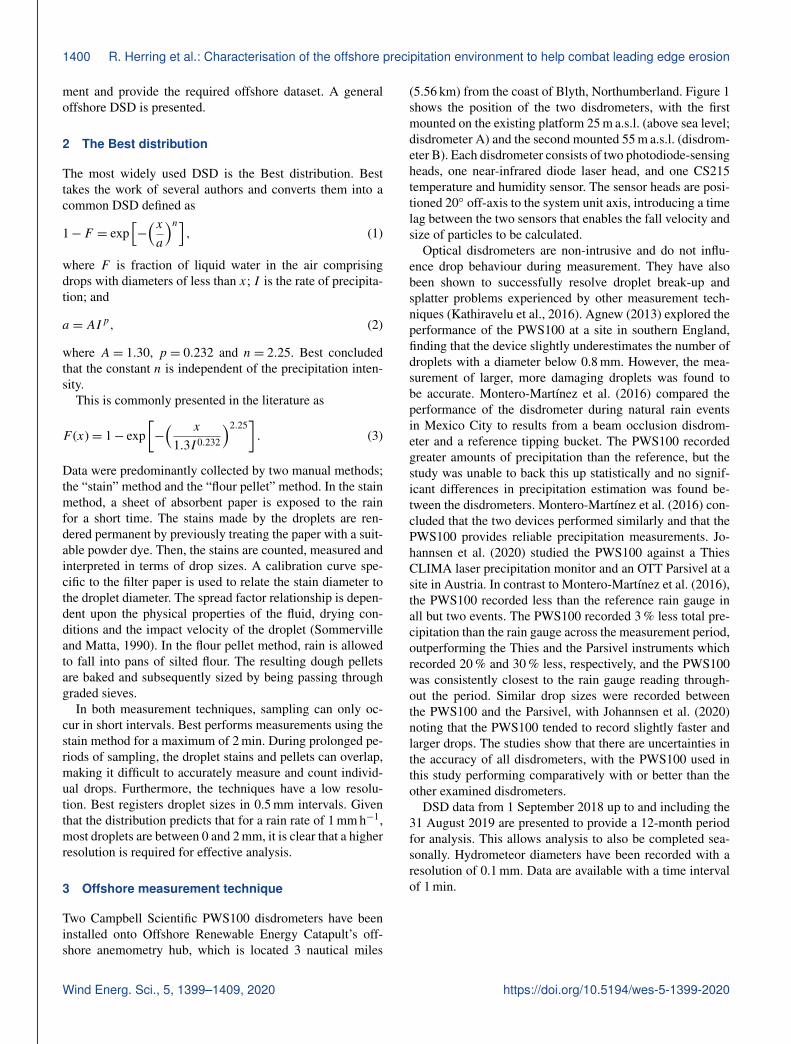
Figure 10 reveals that the Best DSD significantly overesti-mates the diameter of droplets. This is particularly true at thehigher precipitation intensities. The goodness of fit of the off-shore and Best DSDs has been evaluated across the range ofprecipitation intensities in Fig. 11. The offshore DSD alignswell with the raw data and possesses a high coefficient ofdetermination (R2) across the precipitation intensity range.The slight reduction in R2 at higher intensities can be at-tributed to the reduced amount of heavy and violent precipi-tation recorded. The coefficient of determination of the BestDSD reduces significantly as the precipitation intensity in-creases.

5.4 Limitations

The offshore DSD presented has two main limitations.Firstly, the presented measurement period may be a limit-ing factor. As the disdrometer continues to collect data, theDSD can be further refined. Secondly, data have only beencollected at one point. Offshore DSDs may vary from lo-cation to location. To address this, a disdrometer has been

https://doi.org/10.5194/wes-5-1399-2020 Wind Energ. Sci., 5, 1399–1409, 2020

1406 R. Herring et al.: Characterisation of the offshore precipitation environment to help combat leading edge erosion

Figure 10. Comparison between the offshore DSD and the Best DSD at precipitation intensities (a) 0.10005, (b) 0.99612, (c) 2.501,(d) 4.9818, (e) 10.0194 and (f) 19.9687 mm h−1.

positioned at ORE Catapult’s Levenmouth offshore demon-stration turbine for future comparison and validation.

6 Impact of DSD on leading edge erosion lifetimeprediction

The implications of the offshore DSD have been assessedusing the Springer model, which is used by Eisenberg etal. (2018) to predict a protection solution’s in situ life-time from leading edge erosion. The model uses the mediandroplet diameter for a given rain rate to determine the num-ber of impacts to failure, Nic, and the number of impacts on

the blade per square metre per second, N . The number ofimpacts to failure is found from

Nic =8.9d2

(Sec

σo

)5.7

, (9)

where Sec is the effective strength of the protection systemfound from rain erosion test results and σo is the pressure atthe interface between the droplet and protection system andis a function of the droplet diameter and the properties of thesystem relative to the substrate it is applied on. The numberof impacts on the blade per square metre per second is givenas

Wind Energ. Sci., 5, 1399–1409, 2020 https://doi.org/10.5194/wes-5-1399-2020

R. Herring et al.: Characterisation of the offshore precipitation environment to help combat leading edge erosion 1407

Figure 11. Coefficient of determination of the offshore DSD andthe Best DSD across a range of precipitation intensities.

N = qVsβ, (10)

where q is the number of droplets in a cubic metre of air; Vs isthe velocity of the drop impact; and β is the impingementefficiency of the droplets, which is dependent on the aero-foil geometry and droplet diameter. The number of dropletsper cubic metre is found from geometry and is presented bySpringer et al. (1974) as

q = 530.5I

Vtd3 , (11)

where Vt is the terminal velocity of the droplets.The rate of damage, D, from a given precipitation intensity

is found from

D =N

Nic. (12)

The analysis presented here has shown that the Best DSDcurrently used in the Springer model overestimates the sizeof impinging offshore droplets.

The exact number of impacts to failure is dependent onthe protection system and substrate used. For a commercialerosion-resistant polyurethane coating system, the offshoreDSD has been applied to the above equations, and the rela-tive effect on leading edge erosion prediction of the DSD inrelation to the Best DSD is presented in Fig. 12.

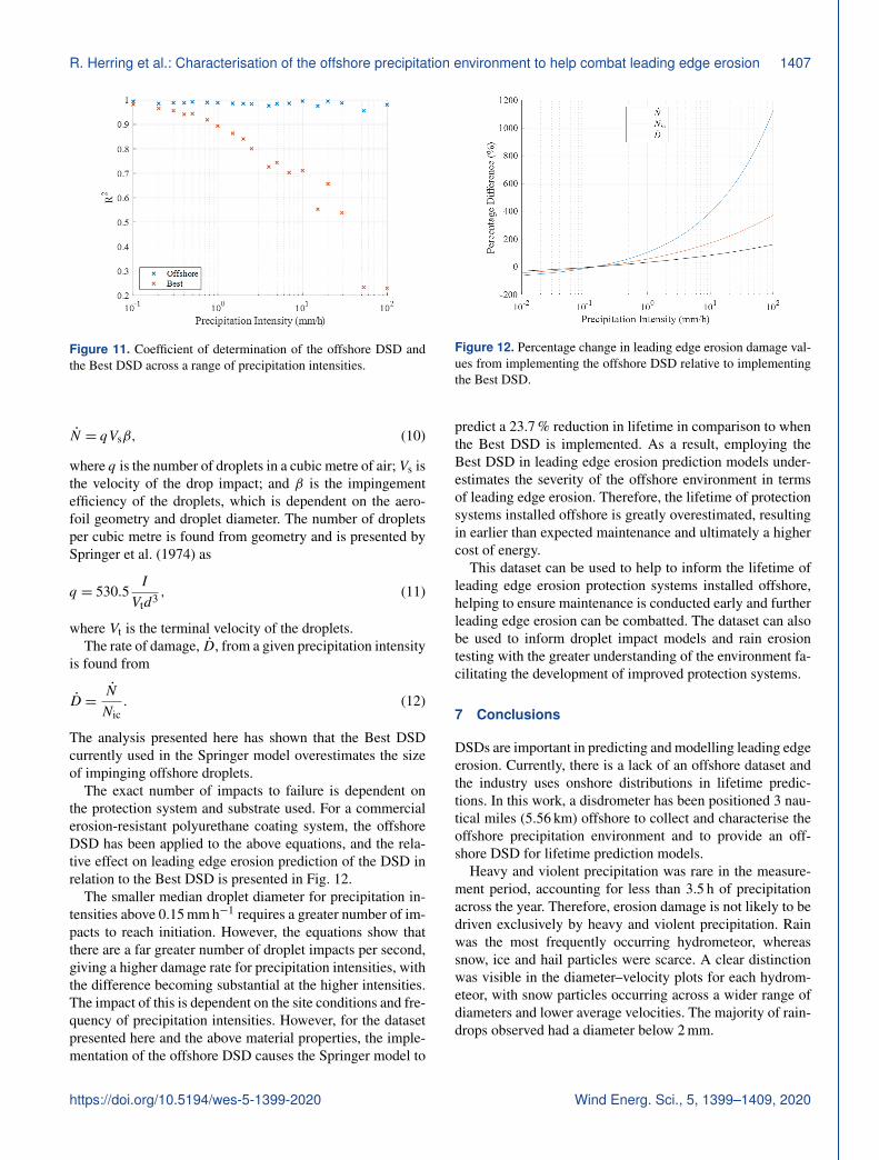
The smaller median droplet diameter for precipitation in-tensities above 0.15 mm h−1 requires a greater number of im-pacts to reach initiation. However, the equations show thatthere are a far greater number of droplet impacts per second,giving a higher damage rate for precipitation intensities, withthe difference becoming substantial at the higher intensities.The impact of this is dependent on the site conditions and fre-quency of precipitation intensities. However, for the datasetpresented here and the above material properties, the imple-mentation of the offshore DSD causes the Springer model to

Figure 12. Percentage change in leading edge erosion damage val-ues from implementing the offshore DSD relative to implementingthe Best DSD.

predict a 23.7 % reduction in lifetime in comparison to whenthe Best DSD is implemented. As a result, employing theBest DSD in leading edge erosion prediction models under-estimates the severity of the offshore environment in termsof leading edge erosion. Therefore, the lifetime of protectionsystems installed offshore is greatly overestimated, resultingin earlier than expected maintenance and ultimately a highercost of energy.

This dataset can be used to help to inform the lifetime ofleading edge erosion protection systems installed offshore,helping to ensure maintenance is conducted early and furtherleading edge erosion can be combatted. The dataset can alsobe used to inform droplet impact models and rain erosiontesting with the greater understanding of the environment fa-cilitating the development of improved protection systems.

7 Conclusions

DSDs are important in predicting and modelling leading edgeerosion. Currently, there is a lack of an offshore dataset andthe industry uses onshore distributions in lifetime predic-tions. In this work, a disdrometer has been positioned 3 nau-tical miles (5.56 km) offshore to collect and characterise theoffshore precipitation environment and to provide an off-shore DSD for lifetime prediction models.

Heavy and violent precipitation was rare in the measure-ment period, accounting for less than 3.5 h of precipitationacross the year. Therefore, erosion damage is not likely to bedriven exclusively by heavy and violent precipitation. Rainwas the most frequently occurring hydrometeor, whereassnow, ice and hail particles were scarce. A clear distinctionwas visible in the diameter–velocity plots for each hydrom-eteor, with snow particles occurring across a wider range ofdiameters and lower average velocities. The majority of rain-drops observed had a diameter below 2 mm.

https://doi.org/10.5194/wes-5-1399-2020 Wind Energ. Sci., 5, 1399–1409, 2020

1408 R. Herring et al.: Characterisation of the offshore precipitation environment to help combat leading edge erosion

A general offshore DSD has been presented. The raw datawere compared to the presented DSD and the most widelyused DSD proposed by Best. A statistical R2 analysis foundthat the offshore DSD aligned well with the data, whereasthe Best DSD significantly overestimated the diameters ofdroplets. The implication of the offshore DSD was evaluatedwith the Springer model, where it was found the inaccura-cies in the Best DSD greatly underestimate the severity ofthe offshore environment in terms of leading edge erosion.As a result, the Best DSD is not a suitable distribution touse in lifetime prediction models for protection systems po-sitioned offshore, and therefore predictions determined usingit are unlikely to be accurate.

The results presented address the lack of an offshoredataset and provide a general offshore DSD that can be usedto inform lifetime prediction models for the offshore envi-ronment. A disdrometer has been placed at ORE Catapult’sLevenmouth offshore wind turbine to provide further infor-mation about the precipitation environment and validate thepresented DSD. The offshore dataset can be used to improveprediction and modelling techniques, helping to inform thedesign of new protection solutions and to combat leadingedge erosion whilst reducing lost energy production and un-expected turbine downtime.

Data availability. Please contact the corresponding author.

Author contributions. RH had the lead on paper writing and dataanalysis and derived conclusions. KD and PH were responsible forinstalling and setting up the disdrometers. KD and CW supervisedthe research.

Competing interests. The authors declare that they have no con-flict of interest.

Special issue statement. This article is part of the special issue“WindEurope Offshore 2019”. It is a result of the WindEurope Off-shore 2019, Copenhagen, Denmark, 26–28 November 2019.

Acknowledgements. This work was supported by the Engi-neering and Physical Sciences Research Council through the EP-SRC Centre for Doctoral Training in Composites Manufacture,project partner the Offshore Renewable Energy Catapult, https://ore.catapult.org.uk (last access: 26 October 2020), and the EPSRCFuture Composites Manufacturing Hub. The authors would also liketo thank the Wind Blade Research Hub for their support in the de-livery of this paper.

Financial support. This research has been supported by the EP-SRC Centre for Doctoral Training in Composites Manufacture(grant no. EP/K50323X/1) and the EPSRC Future CompositesManufacturing Hub (grant no. EP/P006701/1).

Review statement. This paper was edited by Ignacio Marti Perezand reviewed by two anonymous referees.

References

Agnew, J.: Final report on the operation of a Campbell Scien-tific PWS100 present weather sensor at Chilbolton Observatory,Science & Technology Facilities Council, Swindon, UK, 2013.

Bech, J. I., Hasager, C. B., and Bak, C.: Extending the life ofwind turbine blade leading edges by reducing the tip speed dur-ing extreme precipitation events, Wind Energ. Sci., 3, 729–748,https://doi.org/10.5194/wes-3-729-2018, 2018.

Best, A. C.: The size distribution of raindrops, Q. J. Roy. Meteorol.Soc., 76, 16–36, https://doi.org/10.1002/qj.49707632704, 1950.

Brandes, E. A., Zhang, G., and Vivekanandan, J.: Experiments inRainfall Estimation with a Polarimetric Radar in a SubtropicalEnvironment, J. Appl. Meterol., 41, 674–685, 2002.

Chen, B., Wang, J., and Gong, D.: Raindrop Size Distribution ina Midlatitude Continental Squall Line Measured by Thies Opti-cal Disdrometers over East China, J. Appl. Meteorol. Clim., 55,621–634, https://doi.org/10.1175/JAMC-D-15-0127.1, 2016.

Doagou-Rad, S. and Mishnaevsky, L.: Rain erosion of windturbine blades: computational analysis of parameters con-trolling the surface degradation, Meccanica, 55, 725–743,https://doi.org/10.1007/s11012-019-01089-x, 2020.

Eisenberg, D., Laustsen, S., and Stege, J.: Wind turbineblade coating leading edge rain erosion model: De-velopment and validation, Wind Energy, 21, 942–951,https://doi.org/10.1002/we.2200, 2018.

Finans: Siemens sets billions: Ørsted must repairhundreds of turbines, windAction, available at:http://www.windaction.org/posts/47883-siemens-sets-billions-orsted-must-repair-hundreds-of- (last access: 21 October 2019),2018.

Gossard, E. E., Strauch, R. G., Welsh, D. C., and Matrosov, S. Y.:Cloud Layers, Particle Identification and Rain-Rate Profiles fromZRVf Measurements by Clear-Air Doppler Radars, J. Atmos.Ocean. Tech., 9, 108–119, 1992.

Hasager, C., Vejen, F., Bech, J. I., Skrzypinski, W. R., Tilg, A.-M., and Nielsen, M.: Assessment of the rain and wind climatewith focus on wind turbine blade leading edge erosion rate andexpected lifetime in Danish Seas, Renew. Energy, 149, 91–102,https://doi.org/10.1016/j.renene.2019.12.043, 2020.

Jennings, K. S., Winchell, T. S., Livneh, B., and Molotch,N. P.: Spatial variation of the rain-snow temperature thresh-old across the Northern Hemisphere, Nat. Commun., 9, 1–9,https://doi.org/10.1038/s41467-018-03629-7, 2018.

Johannsen, L. L., Zambon, N., Strauss, P., Dostal, T., Zumr,D., Cochrane, T. A., Blöschl, G., Klik, A., Lolk, L.,Zambon, N., Strauss, P., Dostal, T., Zumr, D., Cochrane,T. A., Blöschl, G., and Comparison, A. K.: Comparisonof three types of laser optical disdrometers under nat-

Wind Energ. Sci., 5, 1399–1409, 2020 https://doi.org/10.5194/wes-5-1399-2020

R. Herring et al.: Characterisation of the offshore precipitation environment to help combat leading edge erosion 1409

ural rainfall conditions, Hydrolog. Sci. J., 65, 524–535,https://doi.org/10.1080/02626667.2019.1709641, 2020.

Kathiravelu, G., Lucke, T., and Nichols, P.: Rain DropMeasurement Techniques: A Review, Water, 8, 29,https://doi.org/10.3390/w8010029, 2016.

Keegan, M. H., Nash, D. H., and Stack, M. M.: Modelling RainDrop Impact of Offshore Wind Turbine Blades, in: ASMETurbo Expo 2012: Turbine Technical Conference and Exposi-tion, American Society of Mechanical Engineers, Copenhagen,Denmark, 887–898, 2012.

Met Office: Fact sheet No. 3 – Water in the atmosphere, Devon, UK,2007.

Montero-Martínez, G., Torres-Pérez, E. F. and García-García, F.: A comparison of two optical precipitationsensors with different operating principles: The PWS100and the OAP-2DP, Atmos. Res., 178–179, 550–558,https://doi.org/10.1016/j.atmosres.2016.05.007, 2016.

Slot, H. M., Gelinck, E. R. M., Rentrop, C., and van der Heide,E.: Leading edge erosion of coated wind turbine blades: Re-view of coating life models, Renew. Energy, 80, 837–848,https://doi.org/10.1016/j.renene.2015.02.036, 2015.

Sommerville, D. R. and Matta, J. E.: A method for determingingdroplet size distributions and evaporational losses using paperimpaction cards and dye trackers, Chemical Research Develop-ment & Engineering Center, Maryland, USA, 1990.

Springer, G. S., Yang, C.-I., and Larsen, P. S.: Analysis of RainErosion of Coated Materials, J. Compos. Mater., 8, 229–252,https://doi.org/10.1177/002199837400800302, 1974.

Vejen, F., Tilg, A., Nielsen, M., and Hasager, C.: D1.2 Precipitationstatistics for selected wind farms, Innovationsfonden, Rosekilde,2018.

WeatherSpark: Average Weather in Alnwick, Northum-berland, available at: https://weatherspark.com/y/42298/Average-Weather-in-Alnwick-United-Kingdom-Year-Round,last access: 1 June 2020.

https://doi.org/10.5194/wes-5-1399-2020 Wind Energ. Sci., 5, 1399–1409, 2020