Embed Size (px)
Citation preview

Chapter 5
Sampling-Based Motion Planning
Steven M. LaValle
University of Illinois
Copyright Steven M. LaValle 2006
Available for downloading at http://planning.cs.uiuc.edu/
Published by Cambridge University Press

Chapter 5
Sampling-Based Motion Planning
There are two main philosophies for addressing the motion planning problem, inFormulation 4.1 from Section 4.3.1. This chapter presents one of the philosophies,sampling-based motion planning, which is outlined in Figure 5.1. The main idea isto avoid the explicit construction of Cobs, as described in Section 4.3, and insteadconduct a search that probes the C-space with a sampling scheme. This probingis enabled by a collision detection module, which the motion planning algorithmconsiders as a “black box.” This enables the development of planning algorithmsthat are independent of the particular geometric models. The collision detectionmodule handles concerns such as whether the models are semi-algebraic sets, 3Dtriangles, nonconvex polyhedra, and so on. This general philosophy has been verysuccessful in recent years for solving problems from robotics, manufacturing, andbiological applications that involve thousands and even millions of geometric prim-itives. Such problems would be practically impossible to solve using techniquesthat explicitly represent Cobs.
Notions of completeness It is useful to define several notions of completenessfor sampling-based algorithms. These algorithms have the drawback that theyresult in weaker guarantees that the problem will be solved. An algorithm isconsidered complete if for any input it correctly reports whether there is a solu-
Sampling−BasedMotion Planning AlgorithmCollision
DetectionGeometricModels
DiscreteSearching
C−SpaceSampling
Figure 5.1: The sampling-based planning philosophy uses collision detection asa “black box” that separates the motion planning from the particular geometricand kinematic models. C-space sampling and discrete planning (i.e., searching)are performed.
185
186 S. M. LaValle: Planning Algorithms
tion in a finite amount of time. If a solution exists, it must return one in finitetime. The combinatorial motion planning methods of Chapter 6 will achieve this.Unfortunately, such completeness is not achieved with sampling-based planning.Instead, weaker notions of completeness are tolerated. The notion of densenessbecomes important, which means that the samples come arbitrarily close to anyconfiguration as the number of iterations tends to infinity. A deterministic ap-proach that samples densely will be called resolution complete. This means thatif a solution exists, the algorithm will find it in finite time; however, if a solutiondoes not exist, the algorithm may run forever. Many sampling-based approachesare based on random sampling, which is dense with probability one. This leadsto algorithms that are probabilistically complete, which means that with enoughpoints, the probability that it finds an existing solution converges to one. Themost relevant information, however, is the rate of convergence, which is usuallyvery difficult to establish.
Section 5.1 presents metric and measure space concepts, which are funda-mental to nearly all sampling-based planning algorithms. Section 5.2 presentsgeneral sampling concepts and quality criteria that are effective for analyzing theperformance of sampling-based algorithms. Section 5.3 gives a brief overview ofcollision detection algorithms, to gain an understanding of the information avail-able to a planning algorithm and the computation price that must be paid toobtain it. Section 5.4 presents a framework that defines algorithms which solvemotion planning problems by integrating sampling and discrete planning (i.e.,searching) techniques. These approaches can be considered single query in thesense that a single pair, (qI , qG), is given, and the algorithm must search until itfinds a solution (or it may report early failure). Section 5.5 focuses on rapidlyexploring random trees (RRTs) and rapidly exploring dense trees (RDTs), whichare used to develop efficient single-query planning algorithms. Section 5.6 coversmultiple-query algorithms, which invest substantial preprocessing effort to build adata structure that is later used to obtain efficient solutions for many initial-goalpairs. In this case, it is assumed that the obstacle region O remains the same forevery query.
5.1 Distance and Volume in C-Space
Virtually all sampling-based planning algorithms require a function that measuresthe distance between two points in C. In most cases, this results in a metricspace, which is introduced in Section 5.1.1. Useful examples for motion planningare given in Section 5.1.2. It will also be important in many of these algorithmsto define the volume of a subset of C. This requires a measure space, which isintroduced in Section 5.1.3. Section 5.1.4 introduces invariant measures, whichshould be used whenever possible.

5.1. DISTANCE AND VOLUME IN C-SPACE 187
5.1.1 Metric Spaces
It is straightforward to define Euclidean distance in Rn. To define a distancefunction over any C, however, certain axioms will have to be satisfied so that itcoincides with our expectations based on Euclidean distance.
The following definition and axioms are used to create a function that convertsa topological space into a metric space.1 A metric space (X, ρ) is a topologicalspace X equipped with a function ρ : X ×X → R such that for any a, b, c ∈ X:
1. Nonnegativity: ρ(a, b) ≥ 0.
2. Reflexivity: ρ(a, b) = 0 if and only if a = b.
3. Symmetry: ρ(a, b) = ρ(b, a).
4. Triangle inequality: ρ(a, b) + ρ(b, c) ≥ ρ(a, c).
The function ρ defines distances between points in the metric space, and eachof the four conditions on ρ agrees with our intuitions about distance. The finalcondition implies that ρ is optimal in the sense that the distance from a to c willalways be less than or equal to the total distance obtained by traveling throughan intermediate point b on the way from a to c.
Lp metrics The most important family of metrics over Rn is given for any p ≥ 1as
ρ(x, x′) =
( n∑
i=1
|xi − x′i|p)1/p
. (5.1)
For each value of p, (5.1) is called an Lp metric (pronounced “el pee”). The threemost common cases are
1. L2: The Euclidean metric, which is the familiar Euclidean distance in Rn.
2. L1: The Manhattan metric, which is often nicknamed this way because inR2 it corresponds to the length of a path that is obtained by moving alongan axis-aligned grid. For example, the distance from (0, 0) to (2, 5) is 7 bytraveling “east two blocks” and then “north five blocks”.
3. L∞: The L∞ metric must actually be defined by taking the limit of (5.1) asp tends to infinity. The result is
L∞(x, x′) = max1≤i≤n
{|xi − x′i|}, (5.2)
which seems correct because the larger the value of p, the more the largestterm of the sum in (5.1) dominates.
1Some topological spaces are notmetrizable, which means that no function exists that satisfiesthe axioms. Many metrization theorems give sufficient conditions for a topological space to bemetrizable [75], and virtually any space that has arisen in motion planning will be metrizable.
188 S. M. LaValle: Planning Algorithms
An Lp metric can be derived from a norm on a vector space. An Lp norm overRn is defined as
‖x‖p =( n∑
i=1
|xi|p)1/p
. (5.3)
The case of p = 2 is the familiar definition of the magnitude of a vector, which iscalled the Euclidean norm. For example, assume the vector space is Rn, and let‖ · ‖ be the standard Euclidean norm. The L2 metric is ρ(x, y) = ‖x − y‖. AnyLp metric can be written in terms of a vector subtraction, which is notationallyconvenient.
Metric subspaces By verifying the axioms, it can be shown that any subspaceY ⊂ X of a metric space (X, ρ) itself becomes a metric space by restricting thedomain of ρ to Y ×Y . This conveniently provides metrics on any of the manifoldsand varieties from Chapter 4 by simply using any Lp metric on Rm, the space inwhich the manifold or variety is embedded.
Cartesian products of metric spaces Metrics extend nicely across Cartesianproducts, which is very convenient because C-spaces are often constructed fromCartesian products, especially in the case of multiple bodies. Let (X, ρx) and(Y, ρy) be two metric spaces. A metric space (Z, ρz) can be constructed for theCartesian product Z = X × Y by defining the metric ρz as
ρz(z, z′) = ρz(x, y, x
′, y′) = c1ρx(x, x′) + c2ρy(y, y
′), (5.4)
in which c1 > 0 and c2 > 0 are any positive real constants, and x, x′ ∈ X andy, y′ ∈ Y . Each z ∈ Z is represented as z = (x, y).
Other combinations lead to a metric for Z; for example,
ρz(z, z′) =
(
c1[
ρx(x, x′)]p
+ c2[
ρy(y, y′)]p)1/p
, (5.5)
is a metric for any positive integer p. Once again, two positive constants must bechosen. It is important to understand that many choices are possible, and theremay not necessarily be a “correct” one.
5.1.2 Important Metric Spaces for Motion Planning
This section presents some metric spaces that arise frequently in motion planning.
Example 5.1 (SO(2) Metric Using Complex Numbers) If SO(2) is repre-sented by unit complex numbers, recall that the C-space is the subset of R2 givenby {(a, b) ∈ R2 | a2 + b2 = 1}. Any Lp metric from R2 may be applied. Using theEuclidean metric,
ρ(a1, b1, a2, b2) =√
(a1 − a2)2 + (b1 − b2)2, (5.6)
5.1. DISTANCE AND VOLUME IN C-SPACE 189
for any pair of points (a1, b1) and (a2, b2). �
Example 5.2 (SO(2) Metric by Comparing Angles) You might have noticedthat the previous metric for SO(2) does not give the distance traveling along thecircle. It instead takes a shortcut by computing the length of the line segment inR2 that connects the two points. This distortion may be undesirable. An alterna-tive metric is obtained by directly comparing angles, θ1 and θ2. However, in thiscase special care has to be given to the identification, because there are two waysto reach θ2 from θ1 by traveling along the circle. This causes a min to appear inthe metric definition:
ρ(θ1, θ2) = min{
|θ1 − θ2|, 2π − |θ1 − θ2|}
, (5.7)
for which θ1, θ2 ∈ [0, 2π]/ ∼. This may alternatively be expressed using the com-plex number representation a+ bi as an angle between two vectors:
ρ(a1, b1, a2, b2) = cos−1(a1a2 + b1b2), (5.8)
for two points (a1, b1) and (a2, b2). �
Example 5.3 (An SE(2) Metric) Again by using the subspace principle, ametric can easily be obtained for SE(2). Using the complex number representa-tion of SO(2), each element of SE(2) is a point (xt, yt, a, b) ∈ R4. The Euclideanmetric, or any other Lp metric on R4, can be immediately applied to obtain ametric. �
Example 5.4 (SO(3) Metrics Using Quaternions) As usual, the situation be-comes more complicated for SO(3). The unit quaternions form a subset S3 of R4.Therefore, any Lp metric may be used to define a metric on S3, but this will not bea metric for SO(3) because antipodal points need to be identified. Let h1, h2 ∈ R4
represent two unit quaternions (which are being interpreted here as elements ofR4 by ignoring the quaternion algebra). Taking the identifications into account,the metric is
ρ(h1, h2) = min{
‖h1 − h2‖, ‖h1 + h2‖}
, (5.9)
in which the two arguments of the min correspond to the distances from h1 to h2
and −h2, respectively. The h1 + h2 appears because h2 was negated to yield itsantipodal point, −h2.
As in the case of SO(2), the metric in (5.9) may seem distorted because itmeasures the length of line segments that cut through the interior of S3, as opposedto traveling along the surface. This problem can be fixed to give a very natural
190 S. M. LaValle: Planning Algorithms
metric for SO(3), which is based on spherical linear interpolation. This takesthe line segment that connects the points and pushes it outward onto S3. It iseasier to visualize this by dropping a dimension. Imagine computing the distancebetween two points on S2. If these points lie on the equator, then spherical linearinterpolation yields a distance proportional to that obtained by traveling alongthe equator, as opposed to cutting through the interior of S2 (for points not onthe equator, use the great circle through the points).
It turns out that this metric can easily be defined in terms of the inner productbetween the two quaternions. Recall that for unit vectors v1 and v2 in Rn, v1 ·v2 =cos θ, in which θ is the angle between the vectors. This angle is precisely what isneeded to give the proper distance along S3. The resulting metric is a surprisinglysimple extension of (5.8). The distance along S3 between two quaternions is
ρs(h1, h2) = cos−1(a1a2 + b1b2 + c1c2 + d1d2), (5.10)
in which each hi = (ai, bi, ci, di). Taking identification into account yields themetric
ρ(h1, h2) = min{
ρs(h1, h2), ρs(h1,−h2)}
. (5.11)
�
Example 5.5 (Another SE(2) Metric) For many C-spaces, the problem of re-lating different kinds of quantities arises. For example, any metric defined onSE(2) must compare both distance in the plane and an angular quantity. Forexample, even if c1 = c2 = 1, the range for S1 is [0, 2π) using radians but [0, 360)using degrees. If the same constant c2 is used in either case, two very different met-rics are obtained. The units applied to R2 and S1 are completely incompatible. �
Example 5.6 (Robot Displacement Metric) Sometimes this incompatibilityproblem can be fixed by considering the robot displacement. For any two config-urations q1, q2 ∈ C, a robot displacement metric can be defined as
ρ(q1, q2) = maxa∈A
{
‖a(q1)− a(q2)‖}
, (5.12)
in which a(qi) is the position of the point a in the world when the robot A is atconfiguration qi. Intuitively, the robot displacement metric yields the maximumamount inW that any part of the robot is displaced when moving from configura-tion q1 to q2. The difficulty and efficiency with which this metric can be computeddepend strongly on the particular robot geometric model and kinematics. For aconvex polyhedral robot that can translate and rotate, it is sufficient to checkonly vertices. The metric may appear to be ideal, but efficient algorithms are notknown for most situations. �
5.1. DISTANCE AND VOLUME IN C-SPACE 191
Example 5.7 (Tn Metrics) Next consider making a metric over a torus Tn.The Cartesian product rules such as (5.4) and (5.5) can be extended over everycopy of S1 (one for each parameter θi). This leads to n arbitrary coefficients c1,c2, . . ., cn. Robot displacement could be used to determine the coefficients. Forexample, if the robot is a chain of links, it might make sense to weight changes inthe first link more heavily because the entire chain moves in this case. When thelast parameter is changed, only the last link moves; in this case, it might makesense to give it less weight. �
Example 5.8 (SE(3) Metrics) Metrics for SE(3) can be formed by applyingthe Cartesian product rules to a metric for R3 and a metric for SO(3), such asthat given in (5.11). Again, this unfortunately leaves coefficients to be specified.These issues will arise again in Section 5.3.4, where more details appear on robotdisplacement. �
Pseudometrics Many planning algorithms use functions that behave somewhatlike a distance function but may fail to satisfy all of the metric axioms. If suchdistance functions are used, they will be referred to as pseudometrics. One generalprinciple that can be used to derive pseudometrics is to define the distance to bethe optimal cost-to-go for some criterion (recall discrete cost-to-go functions fromSection 2.3). This will become more important when differential constraints areconsidered in Chapter 14.
In the continuous setting, the cost could correspond to the distance traveledby a robot or even the amount of energy consumed. Sometimes, the resultingpseudometric is not symmetric. For example, it requires less energy for a car totravel downhill as opposed to uphill. Alternatively, suppose that a car is onlycapable of driving forward. It might travel a short distance to go forward fromq1 to some q2, but it might have to travel a longer distance to reach q1 from q2because it cannot drive in reverse. These issues arise for the Dubins car, which iscovered in Sections 13.1.2 and 15.3.1.
An important example of a pseudometric from robotics is a potential function,which is an important part of the randomized potential field method, which isdiscussed in Section 5.4.3. The idea is to make a scalar function that estimatesthe distance to the goal; however, there may be additional terms that attemptto repel the robot away from obstacles. This generally causes local minima toappear in the distance function, which may cause potential functions to violatethe triangle inequality.
192 S. M. LaValle: Planning Algorithms
5.1.3 Basic Measure Theory Definitions
This section briefly indicates how to define volume in a metric space. This providesa basis for defining concepts such as integrals or probability densities. Measuretheory is an advanced mathematical topic that is well beyond the scope of thisbook; however, it is worthwhile to briefly introduce some of the basic definitionsbecause they sometimes arise in sampling-based planning.
Measure can be considered as a function that produces real values for subsetsof a metric space, (X, ρ). Ideally, we would like to produce a nonnegative value,µ(A) ∈ [0,∞], for any subset A ⊆ X. Unfortunately, due to the Banach-Tarskiparadox, if X = Rn, there are some subsets for which trying to assign volumeleads to a contradiction. If X is finite, this cannot happen. Therefore, it is hardto visualize the problem; see [145] for a construction of the bizarre nonmeasurablesets. Due to this problem, a workaround was developed by defining a collection ofsubsets that avoids the paradoxical sets. A collection B of subsets of X is calleda sigma algebra if the following axioms are satisfied:
1. The empty set is in B.
2. If B ∈ B, then X \B ∈ B.
3. For any collection of a countable number of sets in B, their union must alsobe in B.
Note that the last two conditions together imply that the intersection of a count-able number of sets in B is also in B. The sets in B are called the measurablesets.
A nice sigma algebra, called the Borel sets, can be formed from any metricspace (X, ρ) as follows. Start with the set of all open balls in X. These are thesets of the form
B(x, r) = {x′ ∈ X | ρ(x, x′) < r} (5.13)
for any x ∈ X and any r ∈ (0,∞). From the open balls, the Borel sets B arethe sets that can be constructed from these open balls by using the sigma algebraaxioms. For example, an open square in R2 is in B because it can be constructedas the union of a countable number of balls (infinitely many are needed becausethe curved balls must converge to covering the straight square edges). By usingBorel sets, the nastiness of nonmeasurable sets is safely avoided.
Example 5.9 (Borel Sets) A simple example of B can be constructed for R.The open balls are just the set of all open intervals, (x1, x2) ⊂ R, for any x1, x2 ∈ R
such that x1 < x2. �
Using B, a measure µ is now defined as a function µ : B → [0,∞] such thatthe measure axioms are satisfied:

5.1. DISTANCE AND VOLUME IN C-SPACE 193
1. For the empty set, µ(∅) = 0.
2. For any collection, E1, E2, E3, . . ., of a countable (possibly finite) number ofpairwise disjoint, measurable sets, let E denote their union. The measure µmust satisfy
µ(E) =∑
i
µ(Ei), (5.14)
in which i counts over the whole collection.
Example 5.10 (Lebesgue Measure) The most common and important mea-sure is the Lebesgue measure, which becomes the standard notions of length in R,area in R2, and volume in Rn for n ≥ 3. One important concept with Lebesguemeasure is the existence of sets of measure zero. For any countable set A, theLebesgue measure yields µ(A) = 0. For example, what is the total length of thepoint {1} ⊂ R? The length of any single point must be zero. To satisfy the mea-sure axioms, sets such as {1, 3, 4, 5} must also have measure zero. Even infinitesubsets such as Z and Q have measure zero in R. If the dimension of a set A ⊆ Rn
is m for some integer m < n, then µ(A) = 0, according to the Lebesgue measureon Rn. For example, the set S2 ⊂ R3 has measure zero because the sphere hasno volume. However, if the measure space is restricted to S2 and then the surfacearea is defined, then nonzero measure is obtained. �
Example 5.11 (The Counting Measure) If (X, ρ) is finite, then the countingmeasure can be defined. In this case, the measure can be defined over the entirepower set of X. For any A ⊂ X, the counting measure yields µ(A) = |A|, thenumber of elements in A. Verify that this satisfies the measure axioms. �
Example 5.12 (Probability Measure) Measure theory even unifies discreteand continuous probability theory. The measure µ can be defined to yield prob-ability mass. The probability axioms (see Section 9.1.2) are consistent with themeasure axioms, which therefore yield a measure space. The integrals and sumsneeded to define expectations of random variables for continuous and discretecases, respectively, unify into a single measure-theoretic integral. �
Measure theory can be used to define very general notions of integration thatare much more powerful than the Riemann integral that is learned in classicalcalculus. One of the most important concepts is the Lebesgue integral. Insteadof being limited to partitioning the domain of integration into intervals, virtuallyany partition into measurable sets can be used. Its definition requires the notionof a measurable function to ensure that the function domain is partitioned intomeasurable sets. For further study, see [55, 96, 145].
194 S. M. LaValle: Planning Algorithms
5.1.4 Using the Correct Measure
Since many metrics and measures are possible, it may sometimes seem that there isno “correct” choice. This can be frustrating because the performance of sampling-based planning algorithms can depend strongly on these. Conveniently, there is anatural measure, called the Haar measure, for some transformation groups, includ-ing SO(N). Good metrics also follow from the Haar measure, but unfortunately,there are still arbitrary alternatives.
The basic requirement is that the measure does not vary when the sets aretransformed using the group elements. More formally, let G represent a matrixgroup with real-valued entries, and let µ denote a measure on G. If for anymeasurable subset A ⊆ G, and any element g ∈ G, µ(A) = µ(gA) = µ(Ag), thenµ is called the Haar measure2 for G. The notation gA represents the set of allmatrices obtained by the product ga, for any a ∈ A. Similarly, Ag represents allproducts of the form ag.
Example 5.13 (Haar Measure for SO(2)) The Haar measure for SO(2) canbe obtained by parameterizing the rotations as [0, 1]/ ∼ with 0 and 1 identified,and letting µ be the Lebesgue measure on the unit interval. To see the invarianceproperty, consider the interval [1/4, 1/2], which produces a set A ⊂ SO(2) ofrotation matrices. This corresponds to the set of all rotations from θ = π/2 toθ = π. The measure yields µ(A) = 1/4. Now consider multiplying every matrixa ∈ A by a rotation matrix, g ∈ SO(2), to yield Ag. Suppose g is the rotationmatrix for θ = π. The set Ag is the set of all rotation matrices from θ = 3π/2up to θ = 2π = 0. The measure µ(Ag) = 1/4 remains unchanged. Invariancefor gA may be checked similarly. The transformation g translates the intervalsin [0, 1]/ ∼. Since the measure is based on interval lengths, it is invariant withrespect to translation. Note that µ can be multiplied by a fixed constant (such as2π) without affecting the invariance property.
An invariant metric can be defined from the Haar measure on SO(2). For anypoints x1, x2 ∈ [0, 1], let ρ = µ([x1, x2]), in which [x1, x2] is the shortest length(smallest measure) interval that contains x1 and x2 as endpoints. This metric wasalready given in Example 5.2.
To obtain examples that are not the Haar measure, let µ represent probabilitymass over [0, 1] and define any nonuniform probability density function (the uni-form density yields the Haar measure). Any shifting of intervals will change theprobability mass, resulting in a different measure.
Failing to use the Haar measure weights some parts of SO(2) more heavilythan others. Sometimes imposing a bias may be desirable, but it is at least asimportant to know how to eliminate bias. These ideas may appear obvious, butin the case of SO(3) and many other groups it is more challenging to eliminate
2Such a measure is unique up to scale and exists for any locally compact topological group[55, 145].
5.2. SAMPLING THEORY 195
this bias and obtain the Haar measure. �
Example 5.14 (Haar Measure for SO(3)) For SO(3) it turns out once againthat quaternions come to the rescue. If unit quaternions are used, recall thatSO(3) becomes parameterized in terms of S3, but opposite points are identified.It can be shown that the surface area on S3 is the Haar measure. (Since S3 is a 3Dmanifold, it may more appropriately be considered as a surface “volume.”) It willbe seen in Section 5.2.2 that uniform random sampling over SO(3) must be donewith a uniform probability density over S3. This corresponds exactly to the Haarmeasure. If instead SO(3) is parameterized with Euler angles, the Haar measurewill not be obtained. An unintentional bias will be introduced; some rotations inSO(3) will have more weight than others for no particularly good reason. �
5.2 Sampling Theory
5.2.1 Motivation and Basic Concepts
The state space for motion planning, C, is uncountably infinite, yet a sampling-based planning algorithm can consider at most a countable number of samples.If the algorithm runs forever, this may be countably infinite, but in practice weexpect it to terminate early after only considering a finite number of samples.This mismatch between the cardinality of C and the set that can be probed byan algorithm motivates careful consideration of sampling techniques. Once thesampling component has been defined, discrete planning methods from Chapter2 may be adapted to the current setting. Their performance, however, hinges onthe way the C-space is sampled.
Since sampling-based planning algorithms are often terminated early, the par-ticular order in which samples are chosen becomes critical. Therefore, a distinctionis made between a sample set and a sample sequence. A unique sample set canalways be constructed from a sample sequence, but many alternative sequencescan be constructed from one sample set.
Denseness Consider constructing an infinite sample sequence over C. Whatwould be some desirable properties for this sequence? It would be nice if thesequence eventually reached every point in C, but this is impossible because C isuncountably infinite. Strangely, it is still possible for a sequence to get arbitrarilyclose to every element of C (assuming C ⊆ Rm). In topology, this is the notion ofdenseness. Let U and V be any subsets of a topological space. The set U is saidto be dense in V if cl(U) = V (recall the closure of a set from Section 4.1.1). Thismeans adding the boundary points to U produces V . A simple example is that(0, 1) ⊂ R is dense in [0, 1] ⊂ R. A more interesting example is that the set Q of
196 S. M. LaValle: Planning Algorithms
rational numbers is both countable and dense in R. Think about why. For anyreal number, such as π ∈ R, there exists a sequence of fractions that converges toit. This sequence of fractions must be a subset of Q. A sequence (as opposed to aset) is called dense if its underlying set is dense. The bare minimum for samplingmethods is that they produce a dense sequence. Stronger requirements, such asuniformity and regularity, will be explained shortly.
A random sequence is probably dense Suppose that C = [0, 1]. One ofthe simplest ways conceptually to obtain a dense sequence is to pick points atrandom. Suppose I ⊂ [0, 1] is an interval of length e. If k samples are chosenindependently at random,3 the probability that none of them falls into I is (1−e)k.As k approaches infinity, this probability converges to zero. This means that theprobability that any nonzero-length interval in [0, 1] contains no points convergesto zero. One small technicality exists. The infinite sequence of independently,randomly chosen points is only dense with probability one, which is not the same asbeing guaranteed. This is one of the strange outcomes of dealing with uncountablyinfinite sets in probability theory. For example, if a number between [0, 1] ischosen at random, the probably that π/4 is chosen is zero; however, it is stillpossible. (The probability is just the Lebesgue measure, which is zero for a set ofmeasure zero.) For motion planning purposes, this technicality has no practicalimplications; however, if k is not very large, then it might be frustrating to obtainonly probabilistic assurances, as opposed to absolute guarantees of coverage. Thenext sequence is guaranteed to be dense because it is deterministic.
The van der Corput sequence A beautiful yet underutilized sequence waspublished in 1935 by van der Corput, a Dutch mathematician [164]. It exhibitsmany ideal qualities for applications. At the same time, it is based on a simpleidea. Unfortunately, it is only defined for the unit interval. The quest to extendmany of its qualities to higher dimensional spaces motivates the formal qualitymeasures and sampling techniques in the remainder of this section.
To explain the van der Corput sequence, let C = [0, 1]/ ∼, in which 0 ∼ 1,which can be interpreted as SO(2). Suppose that we want to place 16 samples inC. An ideal choice is the set S = {i/16 | 0 ≤ i < 16}, which evenly spaces thepoints at intervals of length 1/16. This means that no point in C is further than1/32 from the nearest sample. What if we want to make S into a sequence? Whatis the best ordering? What if we are not even sure that 16 points are sufficient?Maybe 16 is too few or even too many.
The first two columns of Figure 5.2 show a naive attempt at making S intoa sequence by sorting the points by increasing value. The problem is that afteri = 8, half of C has been neglected. It would be preferable to have a nice coveringof C for any i. Van der Corput’s clever idea was to reverse the order of the bits,when the sequence is represented with binary decimals. In the original sequence,
3See Section 9.1.2 for a review of probability theory.

5.2. SAMPLING THEORY 197
Naive Reverse Van deri Sequence Binary Binary Corput Points in [0, 1]/ ∼1 0 .0000 .0000 02 1/16 .0001 .1000 1/23 1/8 .0010 .0100 1/44 3/16 .0011 .1100 3/45 1/4 .0100 .0010 1/86 5/16 .0101 .1010 5/87 3/8 .0110 .0110 3/88 7/16 .0111 .1110 7/89 1/2 .1000 .0001 1/1610 9/16 .1001 .1001 9/1611 5/8 .1010 .0101 5/1612 11/16 .1011 .1101 13/1613 3/4 .1100 .0011 3/1614 13/16 .1101 .1011 11/1615 7/8 .1110 .0111 7/1616 15/16 .1111 .1111 15/16
Figure 5.2: The van der Corput sequence is obtained by reversing the bits in thebinary decimal representation of the naive sequence.
the most significant bit toggles only once, whereas the least significant bit togglesin every step. By reversing the bits, the most significant bit toggles in every step,which means that the sequence alternates between the lower and upper halves ofC. The third and fourth columns of Figure 5.2 show the original and reversed-order binary representations. The resulting sequence dances around [0, 1]/ ∼ in anice way, as shown in the last two columns of Figure 5.2. Let ν(i) denote the ithpoint of the van der Corput sequence.
In contrast to the naive sequence, each ν(i) lies far away from ν(i + 1). Fur-thermore, the first i points of the sequence, for any i, provide reasonably uniformcoverage of C. When i is a power of 2, the points are perfectly spaced. For otheri, the coverage is still good in the sense that the number of points that appear inany interval of length l is roughly il. For example, when i = 10, every interval oflength 1/2 contains roughly 5 points.
The length, 16, of the naive sequence is actually not important. If instead8 is used, the same ν(1), . . ., ν(8) are obtained. Observe in the reverse binarycolumn of Figure 5.2 that this amounts to removing the last zero from each binarydecimal representation, which does not alter their values. If 32 is used for the naivesequence, then the same ν(1), . . ., ν(16) are obtained, and the sequence continuesnicely from ν(17) to ν(32). To obtain the van der Corput sequence from ν(33) toν(64), six-bit sequences are reversed (corresponding to the case in which the naivesequence has 64 points). The process repeats to produce an infinite sequence that
198 S. M. LaValle: Planning Algorithms
does not require a fixed number of points to be specified a priori. In addition tothe nice uniformity properties for every i, the infinite van der Corput sequence isalso dense in [0, 1]/ ∼. This implies that every open subset must contain at leastone sample.
You have now seen ways to generate nice samples in a unit interval both ran-domly and deterministically. Sections 5.2.2–5.2.4 explain how to generate densesamples with nice properties in the complicated spaces that arise in motion plan-ning.
5.2.2 Random Sampling
Now imagine moving beyond [0, 1] and generating a dense sample sequence for anybounded C-space, C ⊆ Rm. In this section the goal is to generate uniform randomsamples. This means that the probability density function p(q) over C is uniform.Wherever relevant, it also will mean that the probability density is also consistentwith the Haar measure. We will not allow any artificial bias to be introduced byselecting a poor parameterization. For example, picking uniform random Eulerangles does not lead to uniform random samples over SO(3). However, pickinguniform random unit quaternions works perfectly because quaternions use thesame parameterization as the Haar measure; both choose points on S3.
Random sampling is the easiest of all sampling methods to apply to C-spaces.One of the main reasons is that C-spaces are formed from Cartesian products, andindependent random samples extend easily across these products. If X = X1×X2,and uniform random samples x1 and x2 are taken from X1 and X2, respectively,then (x1, x2) is a uniform random sample for X. This is very convenient in im-plementations. For example, suppose the motion planning problem involves 15robots that each translate for any (xt, yt) ∈ [0, 1]2; this yields C = [0, 1]30. Inthis case, 30 points can be chosen uniformly at random from [0, 1] and combinedinto a 30-dimensional vector. Samples generated this way are uniformly randomlydistributed over C. Combining samples over Cartesian products is much moredifficult for nonrandom (deterministic) methods, which are presented in Sections5.2.3 and 5.2.4.
Generating a random element of SO(3) One has to be very careful aboutsampling uniformly over the space of rotations. The probability density mustcorrespond to the Haar measure, which means that a random rotation should beobtained by picking a point at random on S3 and forming the unit quaternion. Anextremely clever way to sample SO(3) uniformly at random is given in [151] andis reproduced here. Choose three points u1, u2, u3 ∈ [0, 1] uniformly at random.A uniform, random quaternion is given by the simple expression
h = (√1− u1 sin 2πu2,
√1− u1 cos 2πu2,
√u1 sin 2πu3,
√u1 cos 2πu3). (5.15)
A full explanation of the method is given in [151], and a brief intuition is givenhere. First drop down a dimension and pick u1, u2 ∈ [0, 1] to generate points
5.2. SAMPLING THEORY 199
on S2. Let u1 represent the value for the third coordinate, (0, 0, u1) ∈ R3. Theslice of points on S2 for which u1 is fixed for 0 < u1 < 1 yields a circle on S2
that corresponds to some line of latitude on S2. The second parameter selectsthe longitude, 2πu2. Fortunately, the points are uniformly distributed over S2.Why? Imagine S2 as the crust on a spherical loaf of bread that is run through abread slicer. The slices are cut in a direction parallel to the equator and are ofequal thickness. The crusts of each slice have equal area; therefore, the points areuniformly distributed. The method proceeds by using that fact that S3 can bepartitioned into a spherical arrangement of circles (known as the Hopf fibration);there is an S1 copy for each point in S2. The method above is used to providea random point on S2 using u2 and u3, and u1 produces a random point on S1;they are carefully combined in (5.15) to yield a random rotation. To respectthe antipodal identification for rotations, any quaternion h found in the lowerhemisphere (i.e., a < 0) can be negated to yield −h. This does not distort theuniform random distribution of the samples.
Generating random directions Some sampling-based algorithms require choos-ing motion directions at random.4 From a configuration q, the possible directionsof motion can be imagined as being distributed around a sphere. In an (n + 1)-dimensional C-space, this corresponds to sampling on Sn. For example, choosinga direction in R2 amounts to picking an element of S1; this can be parameter-ized as θ ∈ [0, 2π]/ ∼. If n = 4, then the previously mentioned trick for SO(3)should be used. If n = 3 or n > 4, then samples can be generated using aslightly more expensive method that exploits spherical symmetries of the multi-dimensional Gaussian density function [54]. The method is explained for Rn+1;boundaries and identifications must be taken into account for other spaces. Foreach of the n + 1 coordinates, generate a sample ui from a zero-mean Gaussiandistribution with the same variance for each coordinate. Following from the Cen-tral Limit Theorem, ui can be approximately obtained by generating k samplesat random over [−1, 1] and adding them (k ≥ 12 is usually sufficient in practice).The vector (u1, u2, . . . , un+1) gives a random direction in Rn+1 because each ui
was obtained independently, and the level sets of the resulting probability densityfunction are spheres. We did not use uniform random samples for each ui becausethis would bias the directions toward the corners of a cube; instead, the Gaussianyields spherical symmetry. The final step is to normalize the vector by takingui/‖u‖ for each coordinate.
Pseudorandom number generation Although there are advantages to uni-form random sampling, there are also several disadvantages. This motivates theconsideration of deterministic alternatives. Since there are trade-offs, it is impor-
4The directions will be formalized in Section 8.3.2 when smooth manifolds are introduced. Inthat case, the directions correspond to the set of possible velocities that have unit magnitude.Presently, the notion of a direction is only given informally.
200 S. M. LaValle: Planning Algorithms
tant to understand how to use both kinds of sampling in motion planning. Oneof the first issues is that computer-generated numbers are not random.5 A pseu-dorandom number generator is usually employed, which is a deterministic methodthat simulates the behavior of randomness. Since the samples are not truly ran-dom, the advantage of extending the samples over Cartesian products does notnecessarily hold. Sometimes problems are caused by unforeseen deterministic de-pendencies. One of the best pseudorandom number generators for avoiding suchtroubles is the Mersenne twister [127], for which implementations can be foundon the Internet.
To help see the general difficulties, the classical linear congruential pseudo-random number generator is briefly explained [109, 134]. The method uses threeinteger parameters, M , a, and c, which are chosen by the user. The first two,M and a, must be relatively prime, meaning that gcd(M,a) = 1. The third pa-rameter, c, must be chosen to satisfy 0 ≤ c < M . Using modular arithmetic, asequence can be generated as
yi+1 = ayi + c mod M, (5.16)
by starting with some arbitrary seed 1 ≤ y0 ≤ M . Pseudorandom numbers in[0, 1] are generated by the sequence
xi = yi/M. (5.17)
The sequence is periodic; therefore, M is typically very large (e.g., M = 231 − 1).Due to periodicity, there are potential problems of regularity appearing in thesamples, especially when applied across a Cartesian product to generate points inRn. Particular values must be chosen for the parameters, and statistical tests areused to evaluate the samples either experimentally or theoretically [134].
Testing for randomness Thus, it is important to realize that even the “ran-dom” samples are deterministic. They are designed to optimize performance onstatistical tests. Many sophisticated statistical tests of uniform randomness areused. One of the simplest, the chi-square test, is described here. This test mea-sures how far computed statistics are from their expected value. As a simpleexample, suppose C = [0, 1]2 and is partitioned into a 10 by 10 array of 100 squareboxes. If a set P of k samples is chosen at random, then intuitively each boxshould receive roughly k/100 of the samples. An error function can be defined tomeasure how far from true this intuition is:
e(P ) =100∑
i=1
(bi − k/100)2, (5.18)
in which bi is the number of samples that fall into box i. It is shown [91] thate(P ) follows a chi-squared distribution. A surprising fact is that the goal is not to
5There are exceptions, which use physical phenomena as a random source [143].

5.2. SAMPLING THEORY 201
minimize e(P ). If the error is too small, we would declare that the samples aretoo uniform to be random! Imagine k = 1, 000, 000 and exactly 10, 000 samplesappear in each of the 100 boxes. This yields e(P ) = 0, but how likely is this toever occur? The error must generally be larger (it appears in many statisticaltables) to account for the irregularity due to randomness.
(a) 196 pseudorandom samples (b) 196 pseudorandom samples
Figure 5.3: Irregularity in a collection of (pseudo)random samples can be nicelyobserved with Voronoi diagrams.
This irregularity can be observed in terms of Voronoi diagrams, as shown inFigure 5.3. The Voronoi diagram partitions R2 into regions based on the samples.Each sample x has an associated Voronoi region Vor(x). For any point y ∈Vor(x), x is the closest sample to y using Euclidean distance. The different sizesand shapes of these regions give some indication of the required irregularity ofrandom sampling. This irregularity may be undesirable for sampling-based motionplanning and is somewhat repaired by the deterministic sampling methods ofSections 5.2.3 and 5.2.4 (however, these methods also have drawbacks).
5.2.3 Low-Dispersion Sampling
This section describes an alternative to random sampling. Here, the goal is tooptimize a criterion called dispersion [134]. Intuitively, the idea is to place samplesin a way that makes the largest uncovered area be as small as possible. Thisgeneralizes of the idea of grid resolution. For a grid, the resolution may be selectedby defining the step size for each axis. As the step size is decreased, the resolutionincreases. If a grid-based motion planning algorithm can increase the resolutionarbitrarily, it becomes resolution complete. Using the concepts in this section,it may instead reduce its dispersion arbitrarily to obtain a resolution complete
202 S. M. LaValle: Planning Algorithms
(a) L2 dispersion (b) L∞ dispersion
Figure 5.4: Reducing the dispersion means reducing the radius of the largestempty ball.
algorithm. Thus, dispersion can be considered as a powerful generalization of thenotion of “resolution.”
Dispersion definition The dispersion6 of a finite set P of samples in a metricspace (X, ρ) is7
δ(P ) = supx∈X
{
minp∈P
{
ρ(x, p)}}
. (5.19)
Figure 5.4 gives an interpretation of the definition for two different metrics.An alternative way to consider dispersion is as the radius of the largest emptyball (for the L∞ metric, the balls are actually cubes). Note that at the boundaryof X (if it exists), the empty ball becomes truncated because it cannot exceedthe boundary. There is also a nice interpretation in terms of Voronoi diagrams.Figure 5.3 can be used to help explain L2 dispersion in R2. The Voronoi verticesare the points at which three or more Voronoi regions meet. These are points inC for which the nearest sample is far. An open, empty disc can be placed at anyVoronoi vertex, with a radius equal to the distance to the three (or more) closestsamples. The radius of the largest disc among those placed at all Voronoi verticesis the dispersion. This interpretation also extends nicely to higher dimensions.
Making good grids Optimizing dispersion forces the points to be distributedmore uniformly over C. This causes them to fail statistical tests, but the pointdistribution is often better for motion planning purposes. Consider the best wayto reduce dispersion if ρ is the L∞ metric and X = [0, 1]n. Suppose that thenumber of samples, k, is given. Optimal dispersion is obtained by partitioning
6The definition is unfortunately backward from intuition. Lower dispersion means that thepoints are nicely dispersed. Thus, more dispersion is bad, which is counterintuitive.
7The sup represents the supremum, which is the least upper bound. If X is closed, then thesup becomes a max. See Section 9.1.1 for more details.

5.2. SAMPLING THEORY 203
(a) 196-point Sukharev grid (b) 196 lattice points
Figure 5.5: The Sukharev grid and a nongrid lattice.
[0, 1] into a grid of cubes and placing a point at the center of each cube, as shownfor n = 2 and k = 196 in Figure 5.5a. The number of cubes per axis must be⌊k 1
n ⌋, in which ⌊·⌋ denotes the floor. If k 1
n is not an integer, then there are leftoverpoints that may be placed anywhere without affecting the dispersion. Notice thatk
1
n just gives the number of points per axis for a grid of k points in n dimensions.The resulting grid will be referred to as a Sukharev grid [158].
The dispersion obtained by the Sukharev grid is the best possible. Therefore,a useful lower bound can be given for any set P of k samples [158]:
δ(P ) ≥ 1
2⌊
k1
d
⌋. (5.20)
This implies that keeping the dispersion fixed requires exponentially many pointsin the dimension, d.
At this point you might wonder why L∞ was used instead of L2, which seemsmore natural. This is because the L2 case is extremely difficult to optimize (exceptin R2, where a tiling of equilateral triangles can be made, with a point in the centerof each one). Even the simple problem of determining the best way to distributea fixed number of points in [0, 1]3 is unsolved for most values of k. See [40] forextensive treatment of this problem.
Suppose now that other topologies are considered instead of [0, 1]n. Let X =[0, 1]/ ∼, in which the identification produces a torus. The situation is quitedifferent because X no longer has a boundary. The Sukharev grid still producesoptimal dispersion, but it can also be shifted without increasing the dispersion.In this case, a standard grid may also be used, which has the same number ofpoints as the Sukharev grid but is translated to the origin. Thus, the first gridpoint is (0, 0), which is actually the same as 2n − 1 other points by identification.If X represents a cylinder and the number of points, k, is given, then it is best tojust use the Sukharev grid. It is possible, however, to shift each coordinate that
204 S. M. LaValle: Planning Algorithms
g1
g2
(a) (b)
Figure 5.6: (a) A distorted grid can even be placed over spheres and SO(3) byputting grids on the faces of an inscribed cube and lifting them to the surface[170]. (b) A lattice can be considered as a grid in which the generators are notnecessarily orthogonal.
behaves like S1. If X is rectangular but not a square, a good grid can still be madeby tiling the space with cubes. In some cases this will produce optimal dispersion.For complicated spaces such as SO(3), no grid exists in the sense defined so far.It is possible, however, to generate grids on the faces of an inscribed Platonic solid[44] and lift the samples to Sn with relatively little distortion [170]. For example,to sample S2, Sukharev grids can be placed on each face of a cube. These arelifted to obtain the warped grid shown in Figure 5.6a.
Example 5.15 (Sukharev Grid) Suppose that n = 2 and k = 9. IfX = [0, 1]2,then the Sukharev grid yields points for the nine cases in which either coordinatemay be 1/6, 1/2, or 5/6. The L∞ dispersion is 1/6. The spacing between the pointsalong each axis is 1/3, which is twice the dispersion. If instead X = [0, 1]2/ ∼,which represents a torus, then the nine points may be shifted to yield the stan-dard grid. In this case each coordinate may be 0, 1/3, or 2/3. The dispersion andspacing between the points remain unchanged. �
One nice property of grids is that they have a lattice structure. This meansthat neighboring points can be obtained very easily be adding or subtractingvectors. Let gj be an n-dimensional vector called a generator. A point on a latticecan be expressed as
x =n
∑
j=1
kjgj (5.21)
for n independent generators, as depicted in Figure 5.6b. In a 2D grid, the gen-erators represent “up” and “right.” If X = [0, 100]2 and a standard grid withinteger spacing is used, then the neighbors of the point (50, 50) are obtained byadding (0, 1), (0,−1), (−1, 0), or (1, 0). In a general lattice, the generators need

5.2. SAMPLING THEORY 205
not be orthogonal. An example is shown in Figure 5.5b. In Section 5.4.2, latticestructure will become important and convenient for defining the search graph.
Infinite grid sequences Now suppose that the number, k, of samples is notgiven. The task is to define an infinite sequence that has the nice properties ofthe van der Corput sequence but works for any dimension. This will become thenotion of a multi-resolution grid. The resolution can be iteratively doubled. For amulti-resolution standard grid in Rn, the sequence will first place one point at theorigin. After 2n points have been placed, there will be a grid with two points peraxis. After 4n points, there will be four points per axis. Thus, after 2ni points forany positive integer i, a grid with 2i points per axis will be represented. If onlycomplete grids are allowed, then it becomes clear why they appear inappropriatefor high-dimensional problems. For example, if n = 10, then full grids appearafter 1, 210, 220, 230, and so on, samples. Each doubling in resolution multipliesthe number of points by 2n. Thus, to use grids in high dimensions, one must bewilling to accept partial grids and define an infinite sequence that places points ina nice way.
The van der Corput sequence can be extended in a straightforward way asfollows. Suppose X = T2 = [0, 1]2/ ∼. The original van der Corput sequencestarted by counting in binary. The least significant bit was used to select whichhalf of [0, 1] was sampled. In the current setting, the two least significant bitscan be used to select the quadrant of [0, 1]2. The next two bits can be used toselect the quadrant within the quadrant. This procedure continues recursively toobtain a complete grid after k = 22i points, for any positive integer i. For anyk, however, there is only a partial grid. The points are distributed with optimalL∞ dispersion. This same idea can be applied in dimension n by using n bits ata time from the binary sequence to select the orthant (n-dimensional quadrant).Many other orderings produce L∞-optimal dispersion. Selecting orderings thatadditionally optimize other criteria, such as discrepancy or L2 dispersion, arecovered in [118, 122]. Unfortunately, it is more difficult to make a multi-resolutionSukharev grid. The base becomes 3 instead of 2; after every 3ni points a completegrid is obtained. For example, in one dimension, the first point appears at 1/2.The next two points appear at 1/6 and 5/6. The next complete one-dimensionalgrid appears after there are 9 points.
Dispersion bounds Since the sample sequence is infinite, it is interesting toconsider asymptotic bounds on dispersion. It is known that for X = [0, 1]n andany Lp metric, the best possible asymptotic dispersion is O(k−1/n) for k pointsand n dimensions [134]. In this expression, k is the variable in the limit and nis treated as a constant. Therefore, any function of n may appear as a constant(i.e., O(f(n)k−1/n) = O(k−1/n) for any positive f(n)). An important practicalconsideration is the size of f(n) in the asymptotic analysis. For example, for thevan der Corput sequence from Section 5.2.1, the dispersion is bounded by 1/k,
206 S. M. LaValle: Planning Algorithms
which means that f(n) = 1. This does not seem good because for values of kthat are powers of two, the dispersion is 1/2k. Using a multi-resolution Sukharevgrid, the constant becomes 3/2 because it takes a longer time before a full grid isobtained. Nongrid, low-dispersion infinite sequences exist that have f(n) = 1/ ln 4[134]; these are not even uniformly distributed, which is rather surprising.
5.2.4 Low-Discrepancy Sampling
In some applications, selecting points that align with the coordinate axis maybe undesirable. Therefore, extensive sampling theory has been developed to de-termine methods that avoid alignments while distributing the points uniformly.In sampling-based motion planning, grids sometimes yield unexpected behaviorbecause a row of points may align nicely with a corridor in Cfree. In some cases, asolution is obtained with surprisingly few samples, and in others, too many sam-ples are necessary. These alignment problems, when they exist, generally drive thevariance higher in computation times because it is difficult to predict when theywill help or hurt. This provides motivation for developing sampling techniquesthat try to reduce this sensitivity.
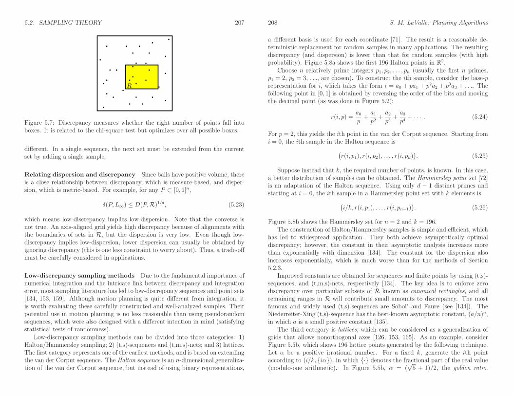
Discrepancy theory and its corresponding sampling methods were developed toavoid these problems for numerical integration [134]. Let X be a measure space,such as [0, 1]n. Let R be a collection of subsets of X that is called a range space.In most cases, R is chosen as the set of all axis-aligned rectangular subsets; hence,this will be assumed from this point onward. With respect to a particular pointset, P , and range space, R, the discrepancy [166] for k samples is defined as (seeFigure 5.7)
D(P,R) = supR∈R
{∣
∣
∣
∣
|P ∩R|k
− µ(R)
µ(X)
∣
∣
∣
∣
}
, (5.22)
in which |P ∩ R| denotes the number of points in P ∩ R. Each term in thesupremum considers how well P can be used to estimate the volume of R. Forexample, if µ(R) is 1/5, then we would hope that about 1/5 of the points in Pfall into R. The discrepancy measures the largest volume estimation error thatcan be obtained over all sets in R.
Asymptotic bounds There are many different asymptotic bounds for discrep-ancy, depending on the particular range space and measure space [126]. The mostwidely referenced bounds are based on the standard range space of axis-alignedrectangular boxes in [0, 1]n. There are two different bounds, depending on whetherthe number of points, k, is given. The best possible asymptotic discrepancy for asingle sequence is O(k−1 logn k). This implies that k is not specified. If, however,for every k a new set of points can be chosen, then the best possible discrepancyis O(k−1 logn−1 k). This bound is lower because it considers the best that can beachieved by a sequence of points sets, in which every point set may be completely
5.2. SAMPLING THEORY 207
R
Figure 5.7: Discrepancy measures whether the right number of points fall intoboxes. It is related to the chi-square test but optimizes over all possible boxes.
different. In a single sequence, the next set must be extended from the currentset by adding a single sample.
Relating dispersion and discrepancy Since balls have positive volume, thereis a close relationship between discrepancy, which is measure-based, and disper-sion, which is metric-based. For example, for any P ⊂ [0, 1]n,
δ(P,L∞) ≤ D(P,R)1/d, (5.23)
which means low-discrepancy implies low-dispersion. Note that the converse isnot true. An axis-aligned grid yields high discrepancy because of alignments withthe boundaries of sets in R, but the dispersion is very low. Even though low-discrepancy implies low-dispersion, lower dispersion can usually be obtained byignoring discrepancy (this is one less constraint to worry about). Thus, a trade-offmust be carefully considered in applications.
Low-discrepancy sampling methods Due to the fundamental importance ofnumerical integration and the intricate link between discrepancy and integrationerror, most sampling literature has led to low-discrepancy sequences and point sets[134, 153, 159]. Although motion planning is quite different from integration, itis worth evaluating these carefully constructed and well-analyzed samples. Theirpotential use in motion planning is no less reasonable than using pseudorandomsequences, which were also designed with a different intention in mind (satisfyingstatistical tests of randomness).
Low-discrepancy sampling methods can be divided into three categories: 1)Halton/Hammersley sampling; 2) (t,s)-sequences and (t,m,s)-nets; and 3) lattices.The first category represents one of the earliest methods, and is based on extendingthe van der Corput sequence. The Halton sequence is an n-dimensional generaliza-tion of the van der Corput sequence, but instead of using binary representations,
208 S. M. LaValle: Planning Algorithms
a different basis is used for each coordinate [71]. The result is a reasonable de-terministic replacement for random samples in many applications. The resultingdiscrepancy (and dispersion) is lower than that for random samples (with highprobability). Figure 5.8a shows the first 196 Halton points in R2.
Choose n relatively prime integers p1, p2, . . . , pn (usually the first n primes,p1 = 2, p2 = 3, . . ., are chosen). To construct the ith sample, consider the base-prepresentation for i, which takes the form i = a0 + pa1 + p2a2 + p3a3 + . . .. Thefollowing point in [0, 1] is obtained by reversing the order of the bits and movingthe decimal point (as was done in Figure 5.2):
r(i, p) =a0p
+a1p2
+a2p3
+a3p4
+ · · · . (5.24)
For p = 2, this yields the ith point in the van der Corput sequence. Starting fromi = 0, the ith sample in the Halton sequence is
(
r(i, p1), r(i, p2), . . . , r(i, pn))
. (5.25)
Suppose instead that k, the required number of points, is known. In this case,a better distribution of samples can be obtained. The Hammersley point set [72]is an adaptation of the Halton sequence. Using only d − 1 distinct primes andstarting at i = 0, the ith sample in a Hammersley point set with k elements is
(
i/k, r(i, p1), . . . , r(i, pn−1))
. (5.26)
Figure 5.8b shows the Hammersley set for n = 2 and k = 196.The construction of Halton/Hammersley samples is simple and efficient, which
has led to widespread application. They both achieve asymptotically optimaldiscrepancy; however, the constant in their asymptotic analysis increases morethan exponentially with dimension [134]. The constant for the dispersion alsoincreases exponentially, which is much worse than for the methods of Section5.2.3.
Improved constants are obtained for sequences and finite points by using (t,s)-sequences, and (t,m,s)-nets, respectively [134]. The key idea is to enforce zerodiscrepancy over particular subsets of R known as canonical rectangles, and allremaining ranges in R will contribute small amounts to discrepancy. The mostfamous and widely used (t,s)-sequences are Sobol’ and Faure (see [134]). TheNiederreiter-Xing (t,s)-sequence has the best-known asymptotic constant, (a/n)n,in which a is a small positive constant [135].
The third category is lattices, which can be considered as a generalization ofgrids that allows nonorthogonal axes [126, 153, 165]. As an example, considerFigure 5.5b, which shows 196 lattice points generated by the following technique.Let α be a positive irrational number. For a fixed k, generate the ith pointaccording to (i/k, {iα}), in which {·} denotes the fractional part of the real value(modulo-one arithmetic). In Figure 5.5b, α = (
√5 + 1)/2, the golden ratio.

5.3. COLLISION DETECTION 209
(a) 196 Halton points (b) 196 Hammersley points
Figure 5.8: The Halton and Hammersley points are easy to construct and providea nice alternative to random sampling that achieves more regularity. Comparethe Voronoi regions to those in Figure 5.3. Beware that although these sequencesproduce asymptotically optimal discrepancy, their performance degrades substan-tially in higher dimensions (e.g., beyond 10).
This procedure can be generalized to n dimensions by picking n − 1 distinctirrational numbers. A technique for choosing the α parameters by using the rootsof irreducible polynomials is discussed in [126]. The ith sample in the lattice is
(
i
k, {iα1}, . . . , {iαn−1}
)
. (5.27)
Recent analysis shows that some lattice sets achieve asymptotic discrepancythat is very close to that of the best-known nonlattice sample sets [73, 160].Thus, restricting the points to lie on a lattice seems to entail little or no loss inperformance, but has the added benefit of a regular neighborhood structure thatis useful for path planning. Historically, lattices have required the specificationof k in advance; however, there has been increasing interest in extensible lattices,which are infinite sequences [74, 160].
5.3 Collision Detection
Once it has been decided where the samples will be placed, the next problem is todetermine whether the configuration is in collision. Thus, collision detection is acritical component of sampling-based planning. Even though it is often treated asa black box, it is important to study its inner workings to understand the informa-tion it provides and its associated computational cost. In most motion planningapplications, the majority of computation time is spent on collision checking.
210 S. M. LaValle: Planning Algorithms
A variety of collision detection algorithms exist, ranging from theoretical algo-rithms that have excellent computational complexity to heuristic, practical algo-rithms whose performance is tailored to a particular application. The techniquesfrom Section 4.3 can be used to develop a collision detection algorithm by defininga logical predicate using the geometric model of Cobs. For the case of a 2D worldwith a convex robot and obstacle, this leads to an linear-time collision detectionalgorithm. In general, however, it can be determined whether a configuration isin collision more efficiently by avoiding the full construction of Cobs.
5.3.1 Basic Concepts
As in Section 3.1.1, collision detection may be viewed as a logical predicate. Inthe current setting it appears as φ : C → {true, false}, in which the domain isC instead of W . If q ∈ Cobs, then φ(q) = true; otherwise, φ(q) = false.
Distance between two sets For the Boolean-valued function φ, there is noinformation about how far the robot is from hitting the obstacles. Such informa-tion is very important in planning algorithms. A distance function provides thisinformation and is defined as d : C → [0,∞), in which the real value in the rangeof f indicates the distance in the world, W , between the closest pair of pointsover all pairs from A(q) and O. In general, for two closed, bounded subsets, Eand F , of Rn, the distance is defined as
ρ(E,F ) = mine∈E
{
minf∈F
{
‖e− f‖}}
, (5.28)
in which ‖ · ‖ is the Euclidean norm. Clearly, if E ∩ F 6= ∅, then ρ(E,F ) = 0.The methods described in this section may be used to either compute distanceor only determine whether q ∈ Cobs. In the latter case, the computation is oftenmuch faster because less information is required.
Two-phase collision detection Suppose that the robot is a collection of mattached links, A1, A2, . . ., Am, and that O has k connected components. For thiscomplicated situation, collision detection can be viewed as a two-phase process.
1. Broad Phase: In the broad phase, the task is to avoid performing expensivecomputations for bodies that are far away from each other. Simple bound-ing boxes can be placed around each of the bodies, and simple tests can beperformed to avoid costly collision checking unless the boxes overlap. Hash-ing schemes can be employed in some cases to greatly reduce the numberof pairs of boxes that have to be tested for overlap [133]. For a robot thatconsists of multiple bodies, the pairs of bodies that should be considered forcollision must be specified in advance, as described in Section 4.3.1.
5.3. COLLISION DETECTION 211
(a) (b) (c) (d)
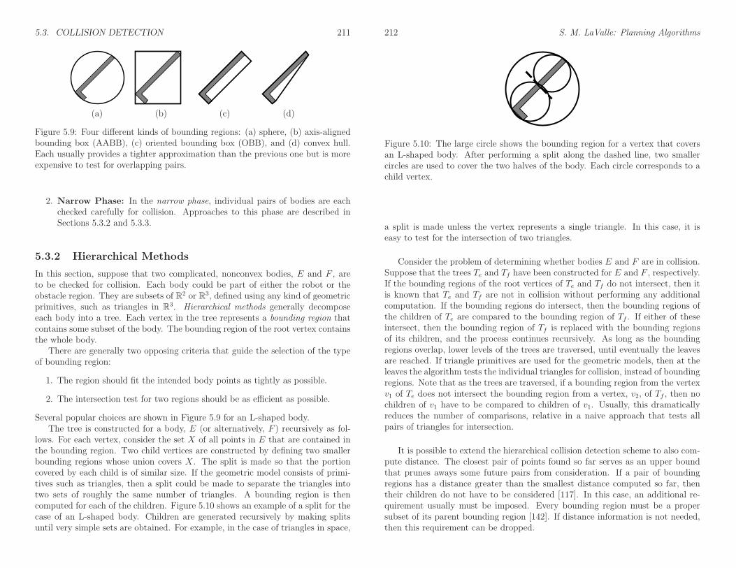
Figure 5.9: Four different kinds of bounding regions: (a) sphere, (b) axis-alignedbounding box (AABB), (c) oriented bounding box (OBB), and (d) convex hull.Each usually provides a tighter approximation than the previous one but is moreexpensive to test for overlapping pairs.
2. Narrow Phase: In the narrow phase, individual pairs of bodies are eachchecked carefully for collision. Approaches to this phase are described inSections 5.3.2 and 5.3.3.
5.3.2 Hierarchical Methods
In this section, suppose that two complicated, nonconvex bodies, E and F , areto be checked for collision. Each body could be part of either the robot or theobstacle region. They are subsets of R2 or R3, defined using any kind of geometricprimitives, such as triangles in R3. Hierarchical methods generally decomposeeach body into a tree. Each vertex in the tree represents a bounding region thatcontains some subset of the body. The bounding region of the root vertex containsthe whole body.
There are generally two opposing criteria that guide the selection of the typeof bounding region:
1. The region should fit the intended body points as tightly as possible.
2. The intersection test for two regions should be as efficient as possible.
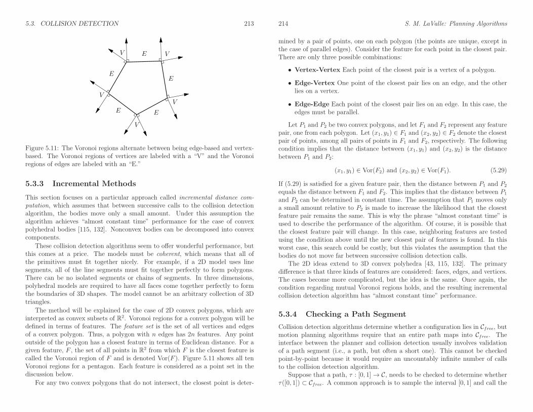
Several popular choices are shown in Figure 5.9 for an L-shaped body.The tree is constructed for a body, E (or alternatively, F ) recursively as fol-
lows. For each vertex, consider the set X of all points in E that are contained inthe bounding region. Two child vertices are constructed by defining two smallerbounding regions whose union covers X. The split is made so that the portioncovered by each child is of similar size. If the geometric model consists of primi-tives such as triangles, then a split could be made to separate the triangles intotwo sets of roughly the same number of triangles. A bounding region is thencomputed for each of the children. Figure 5.10 shows an example of a split for thecase of an L-shaped body. Children are generated recursively by making splitsuntil very simple sets are obtained. For example, in the case of triangles in space,
212 S. M. LaValle: Planning Algorithms
Figure 5.10: The large circle shows the bounding region for a vertex that coversan L-shaped body. After performing a split along the dashed line, two smallercircles are used to cover the two halves of the body. Each circle corresponds to achild vertex.
a split is made unless the vertex represents a single triangle. In this case, it iseasy to test for the intersection of two triangles.
Consider the problem of determining whether bodies E and F are in collision.Suppose that the trees Te and Tf have been constructed for E and F , respectively.If the bounding regions of the root vertices of Te and Tf do not intersect, then itis known that Te and Tf are not in collision without performing any additionalcomputation. If the bounding regions do intersect, then the bounding regions ofthe children of Te are compared to the bounding region of Tf . If either of theseintersect, then the bounding region of Tf is replaced with the bounding regionsof its children, and the process continues recursively. As long as the boundingregions overlap, lower levels of the trees are traversed, until eventually the leavesare reached. If triangle primitives are used for the geometric models, then at theleaves the algorithm tests the individual triangles for collision, instead of boundingregions. Note that as the trees are traversed, if a bounding region from the vertexv1 of Te does not intersect the bounding region from a vertex, v2, of Tf , then nochildren of v1 have to be compared to children of v1. Usually, this dramaticallyreduces the number of comparisons, relative in a naive approach that tests allpairs of triangles for intersection.
It is possible to extend the hierarchical collision detection scheme to also com-pute distance. The closest pair of points found so far serves as an upper boundthat prunes aways some future pairs from consideration. If a pair of boundingregions has a distance greater than the smallest distance computed so far, thentheir children do not have to be considered [117]. In this case, an additional re-quirement usually must be imposed. Every bounding region must be a propersubset of its parent bounding region [142]. If distance information is not needed,then this requirement can be dropped.
5.3. COLLISION DETECTION 213
V
V
V
E
E
E
V
E
E
V
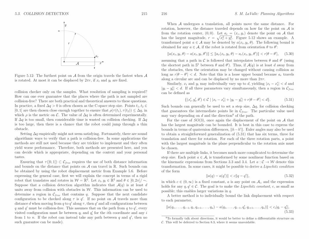
Figure 5.11: The Voronoi regions alternate between being edge-based and vertex-based. The Voronoi regions of vertices are labeled with a “V” and the Voronoiregions of edges are labeled with an “E.”
5.3.3 Incremental Methods
This section focuses on a particular approach called incremental distance com-putation, which assumes that between successive calls to the collision detectionalgorithm, the bodies move only a small amount. Under this assumption thealgorithm achieves “almost constant time” performance for the case of convexpolyhedral bodies [115, 132]. Nonconvex bodies can be decomposed into convexcomponents.
These collision detection algorithms seem to offer wonderful performance, butthis comes at a price. The models must be coherent, which means that all ofthe primitives must fit together nicely. For example, if a 2D model uses linesegments, all of the line segments must fit together perfectly to form polygons.There can be no isolated segments or chains of segments. In three dimensions,polyhedral models are required to have all faces come together perfectly to formthe boundaries of 3D shapes. The model cannot be an arbitrary collection of 3Dtriangles.
The method will be explained for the case of 2D convex polygons, which areinterpreted as convex subsets of R2. Voronoi regions for a convex polygon will bedefined in terms of features. The feature set is the set of all vertices and edgesof a convex polygon. Thus, a polygon with n edges has 2n features. Any pointoutside of the polygon has a closest feature in terms of Euclidean distance. For agiven feature, F , the set of all points in R2 from which F is the closest feature iscalled the Voronoi region of F and is denoted Vor(F ). Figure 5.11 shows all tenVoronoi regions for a pentagon. Each feature is considered as a point set in thediscussion below.
For any two convex polygons that do not intersect, the closest point is deter-
214 S. M. LaValle: Planning Algorithms
mined by a pair of points, one on each polygon (the points are unique, except inthe case of parallel edges). Consider the feature for each point in the closest pair.There are only three possible combinations:
• Vertex-Vertex Each point of the closest pair is a vertex of a polygon.
• Edge-Vertex One point of the closest pair lies on an edge, and the otherlies on a vertex.
• Edge-Edge Each point of the closest pair lies on an edge. In this case, theedges must be parallel.
Let P1 and P2 be two convex polygons, and let F1 and F2 represent any featurepair, one from each polygon. Let (x1, y1) ∈ F1 and (x2, y2) ∈ F2 denote the closestpair of points, among all pairs of points in F1 and F2, respectively. The followingcondition implies that the distance between (x1, y1) and (x2, y2) is the distancebetween P1 and P2:
(x1, y1) ∈ Vor(F2) and (x2, y2) ∈ Vor(F1). (5.29)
If (5.29) is satisfied for a given feature pair, then the distance between P1 and P2
equals the distance between F1 and F2. This implies that the distance between P1
and P2 can be determined in constant time. The assumption that P1 moves onlya small amount relative to P2 is made to increase the likelihood that the closestfeature pair remains the same. This is why the phrase “almost constant time” isused to describe the performance of the algorithm. Of course, it is possible thatthe closest feature pair will change. In this case, neighboring features are testedusing the condition above until the new closest pair of features is found. In thisworst case, this search could be costly, but this violates the assumption that thebodies do not move far between successive collision detection calls.
The 2D ideas extend to 3D convex polyhedra [43, 115, 132]. The primarydifference is that three kinds of features are considered: faces, edges, and vertices.The cases become more complicated, but the idea is the same. Once again, thecondition regarding mutual Voronoi regions holds, and the resulting incrementalcollision detection algorithm has “almost constant time” performance.
5.3.4 Checking a Path Segment
Collision detection algorithms determine whether a configuration lies in Cfree, butmotion planning algorithms require that an entire path maps into Cfree. Theinterface between the planner and collision detection usually involves validationof a path segment (i.e., a path, but often a short one). This cannot be checkedpoint-by-point because it would require an uncountably infinite number of callsto the collision detection algorithm.
Suppose that a path, τ : [0, 1]→ C, needs to be checked to determine whetherτ([0, 1]) ⊂ Cfree. A common approach is to sample the interval [0, 1] and call the
5.3. COLLISION DETECTION 215
A x
y
ar
r
Figure 5.12: The furthest point on A from the origin travels the fastest when Ais rotated. At most it can be displaced by 2πr, if xt and yt are fixed.
collision checker only on the samples. What resolution of sampling is required?How can one ever guarantee that the places where the path is not sampled arecollision-free? There are both practical and theoretical answers to these questions.In practice, a fixed ∆q > 0 is often chosen as the C-space step size. Points t1, t2 ∈[0, 1] are then chosen close enough together to ensure that ρ(τ(t1), τ(t2)) ≤ ∆q, inwhich ρ is the metric on C. The value of ∆q is often determined experimentally.If ∆q is too small, then considerable time is wasted on collision checking. If ∆qis too large, then there is a chance that the robot could jump through a thinobstacle.
Setting ∆q empirically might not seem satisfying. Fortunately, there are soundalgorithmic ways to verify that a path is collision-free. In some applications themethods are still not used because they are trickier to implement and they oftenyield worse performance. Therefore, both methods are presented here, and youcan decide which is appropriate, depending on the context and your personaltastes.
Ensuring that τ([0, 1]) ⊂ Cfree requires the use of both distance informationand bounds on the distance that points on A can travel in R. Such bounds canbe obtained by using the robot displacement metric from Example 5.6. Beforeexpressing the general case, first we will explain the concept in terms of a rigidrobot that translates and rotates in W = R2. Let xt, yt ∈ R2 and θ ∈ [0, 2π]/ ∼.Suppose that a collision detection algorithm indicates that A(q) is at least dunits away from collision with obstacles in W . This information can be used todetermine a region in Cfree that contains q. Suppose that the next candidateconfiguration to be checked along τ is q′. If no point on A travels more thandistance d when moving from q to q′ along τ , then q′ and all configurations betweenq and q′ must be collision-free. This assumes that on the path from q to q′, everyvisited configuration must lie between qi and q′i for the ith coordinate and any ifrom 1 to n. If the robot can instead take any path between q and q′, then nosuch guarantee can be made).
216 S. M. LaValle: Planning Algorithms
When A undergoes a translation, all points move the same distance. Forrotation, however, the distance traveled depends on how far the point on A isfrom the rotation center, (0, 0). Let ar = (xr, yr) denote the point on A thathas the largest magnitude, r =
√
x2r + y2r . Figure 5.12 shows an example. A
transformed point a ∈ A may be denoted by a(xt, yt, θ). The following bound isobtained for any a ∈ A, if the robot is rotated from orientation θ to θ′:
‖a(xt, yt, θ)− a(xt, yt, θ′)‖ ≤ ‖ar(xt, yt, θ)− ar(xt, yt, θ
′)‖ < r|θ − θ′|, (5.30)
assuming that a path in C is followed that interpolates between θ and θ′ (usingthe shortest path in S1 between θ and θ′). Thus, if A(q) is at least d away fromthe obstacles, then the orientation may be changed without causing collision aslong as r|θ − θ′| < d. Note that this is a loose upper bound because ar travelsalong a circular arc and can be displaced by no more than 2πr.
Similarly, xt and yt may individually vary up to d, yielding |xt − x′t| < d and
|yt − y′t| < d. If all three parameters vary simultaneously, then a region in Cfreecan be defined as
{(x′t, y
′t, θ
′) ∈ C | |xt − x′t|+ |yt − y′t|+ r|θ − θ′| < d}. (5.31)
Such bounds can generally be used to set a step size, ∆q, for collision checkingthat guarantees the intermediate points lie in Cfree. The particular value usedmay vary depending on d and the direction8 of the path.
For the case of SO(3), once again the displacement of the point on A thathas the largest magnitude can be bounded. It is best in this case to express thebounds in terms of quaternion differences, ‖h−h′‖. Euler angles may also be usedto obtain a straightforward generalization of (5.31) that has six terms, three fortranslation and three for rotation. For each of the three rotation parts, a pointwith the largest magnitude in the plane perpendicular to the rotation axis mustbe chosen.
If there are multiple links, it becomes much more complicated to determine thestep size. Each point a ∈ Ai is transformed by some nonlinear function based onthe kinematic expressions from Sections 3.3 and 3.4. Let a : C → W denote thistransformation. In some cases, it might be possible to derive a Lipschitz conditionof the form
‖a(q)− a(q′)‖ < c‖q − q′‖, (5.32)
in which c ∈ (0,∞) is a fixed constant, a is any point on Ai, and the expressionholds for any q, q′ ∈ C. The goal is to make the Lipschitz constant, c, as small aspossible; this enables larger variations in q.
A better method is to individually bound the link displacement with respectto each parameter,
‖a(q1, . . . , qi−1, qi, qi+1, . . . , qn)− a(q1, . . . , qi−1, q′i, qi+1, . . . , qn)‖ < ci|qi − q′i|,
(5.33)
8To formally talk about directions, it would be better to define a differentiable structure onC. This will be deferred to Section 8.3, where it seems unavoidable.

5.4. INCREMENTAL SAMPLING AND SEARCHING 217
to obtain the Lipschitz constants c1, . . ., cn. The bound on robot displacementbecomes
‖a(q)− a(q′)‖ <n
∑
i=1
ci|qi − q′i|. (5.34)
The benefit of using individual parameter bounds can be seen by considering a longchain. Consider a 50-link chain of line segments in R2, and each link has length10. The C-space is T50, which can be parameterized as [0, 2π]50/ ∼. Suppose thatthe chain is in a straight-line configuration (θi = 0 for all 1 ≤ i ≤ 50), whichmeans that the last point is at (500, 0) ∈ W . Changes in θ1, the orientation ofthe first link, dramatically move A50. However, changes in θ50 move A50 a smalleramount. Therefore, it is advantageous to pick a different ∆qi for each 1 ≤ i ≤ 50.In this example, a smaller value should be used for ∆θ1 in comparison to ∆θ50.
Unfortunately, there are more complications. Suppose the 50-link chain isin a configuration that folds all of the links on top of each other (θi = π foreach 1 ≤ i ≤ n). In this case, A50 does not move as fast when θ1 is perturbed,in comparison to the straight-line configuration. A larger step size for θ1 couldbe used for this configuration, relative to other parts of C. The implication isthat, although Lipschitz constants can be made to hold over all of C, it might bepreferable to determine a better bound in a local region around q ∈ C. A linearmethod could be obtained by analyzing the Jacobian of the transformations, suchas (3.53) and (3.57).
Another important concern when checking a path is the order in which thesamples are checked. For simplicity, suppose that ∆q is constant and that the pathis a constant-speed parameterization. Should the collision checker step along from0 up to 1? Experimental evidence indicates that it is best to use a recursive binarystrategy [59]. This makes no difference if the path is collision-free, but it oftensaves time if the path is in collision. This is a kind of sampling problem over[0, 1], which is addressed nicely by the van der Corput sequence, ν. The lastcolumn in Figure 5.2 indicates precisely where to check along the path in eachstep. Initially, τ(1) is checked. Following this, points from the van der Corputsequence are checked in order: τ(0), τ(1/2), τ(1/4), τ(3/4), τ(1/8), . . .. Theprocess terminates if a collision is found or when the dispersion falls below ∆q.If ∆q is not constant, then it is possible to skip over some points of ν in regionswhere the allowable variation in q is larger.
5.4 Incremental Sampling and Searching
5.4.1 The General Framework
The algorithms of Sections 5.4 and 5.5 follow the single-query model, which means(qI , qG) is given only once per robot and obstacle set. This means that there are noadvantages to precomputation, and the sampling-based motion planning problem
218 S. M. LaValle: Planning Algorithms
can be considered as a kind of search. The multiple-query model, which favorsprecomputation, is covered in Section 5.6.
The sampling-based planning algorithms presented in the present section arestrikingly similar to the family of search algorithms summarized in Section 2.2.4.The main difference lies in step 3 below, in which applying an action, u, is replacedby generating a path segment, τs. Another difference is that the search graph, G,is undirected, with edges that represent paths, as opposed to a directed graph inwhich edges represent actions. It is possible to make these look similar by definingan action space for motion planning that consists of a collection of paths, but thisis avoided here. In the case of motion planning with differential constraints, thiswill actually be required; see Chapter 14.
Most single-query, sampling-based planning algorithms follow this template:
1. Initialization: Let G(V,E) represent an undirected search graph, for whichV contains at least one vertex and E contains no edges. Typically, V con-tains qI , qG, or both. In general, other points in Cfree may be included.
2. Vertex Selection Method (VSM): Choose a vertex qcur ∈ V for expan-sion.
3. Local Planning Method (LPM): For some qnew ∈ Cfree that may ormay not be represented by a vertex in V , attempt to construct a pathτs : [0, 1]→ Cfree such that τ(0) = qcur and τ(1) = qnew. Using the methodsof Section 5.3.4, τs must be checked to ensure that it does not cause acollision. If this step fails to produce a collision-free path segment, then goto step 2.
4. Insert an Edge in the Graph: Insert τs into E, as an edge from qcur toqnew. If qnew is not already in V , then it is inserted.
5. Check for a Solution: Determine whether G encodes a solution path.As in the discrete case, if there is a single search tree, then this is trivial;otherwise, it can become complicated and expensive.
6. Return to Step 2: Iterate unless a solution has been found or some ter-mination condition is satisfied, in which case the algorithm reports failure.
In the present context, G is a topological graph, as defined in Example 4.6.Each vertex is a configuration and each edge is a path that connects two configu-rations. In this chapter, it will be simply referred to as a graph when there is nochance of confusion. Some authors refer to such a graph as a roadmap; however,we reserve the term roadmap for a graph that contains enough paths to make anymotion planning query easily solvable. This case is covered in Section 5.6 andthroughout Chapter 6.
A large family of sampling-based algorithms can be described by varying theimplementations of steps 2 and 3. Implementations of the other steps may also

5.4. INCREMENTAL SAMPLING AND SEARCHING 219
qIqG
qI qG
(a) (b)
qGqI
qGqI
(c) (d)
Figure 5.13: All of these depict high-dimensional obstacle regions in C-space. (a)The search must involve some sort of multi-resolution aspect, otherwise, that al-gorithm may explore too many points within a cavity. (b) Sometimes the problemis like a bug trap, in which case bidirectional search can help. (c) For a doublebug trap, multi-directional search may be needed. (d) This example is hard tosolve even for multi-directional search.
vary, but this is less important and will be described where appropriate. Forconvenience, step 2 will be called the vertex selection method (VSM) and step 3will be called the local planning method (LPM). The role of the VSM is similar tothat of the priority queue, Q, in Section 2.2.1. The role of the LPM is to computea collision-free path segment that can be added to the graph. It is called localbecause the path segment is usually simple (e.g., the shortest path) and travels ashort distance. It is not global in the sense that the LPM does not try to solve theentire planning problem; it is expected that the LPM may often fail to constructpath segments.
It will be formalized shortly, but imagine for the time being that any of thesearch algorithms from Section 2.2 may be applied to motion planning by ap-proximating C with a high-resolution grid. The resulting problem looks like amulti-dimensional extension of Example 2.1 (the “labyrinth” walls are formedby Cobs). For a high-resolution grid in a high-dimensional space, most classicaldiscrete searching algorithms have trouble getting trapped in a local minimum.There could be an astronomical number of configurations that fall within a con-
220 S. M. LaValle: Planning Algorithms
cavity in Cobs that must be escaped to solve the problem, as shown in Figure5.13a. Imagine a problem in which the C-space obstacle is a giant “bowl” thatcan trap the configuration. This figure is drawn in two dimensions, but imaginethat the C has many dimensions, such as six for SE(3) or perhaps dozens for alinkage. If the discrete planning algorithms from Section 2.2 are applied to a high-resolution grid approximation of C, then they will all waste their time filling upthe bowl before being able to escape to qG. The number of grid points in this bowlwould typically be on the order of 100n for an n-dimensional C-space. Therefore,sampling-based motion planning algorithms combine sampling and searching in away that attempts to overcome this difficulty.
As in the case of discrete search algorithms, there are several classes of algo-rithms based on the number of search trees.
Unidirectional (single-tree) methods: In this case, the planning ap-pears very similar to discrete forward search, which was given in Figure 2.4.The main difference between algorithms in this category is how they imple-ment the VSM and LPM. Figure 5.13b shows a bug trap9 example for whichforward-search algorithms would have great trouble; however, the problemmight not be difficult for backward search, if the planner incorporates somekind of greedy, best-first behavior. This example, again in high dimensions,can be considered as a kind of “bug trap.” To leave the trap, a path mustbe found from qI into the narrow opening. Imagine a fly buzzing aroundthrough the high-dimensional trap. The escape opening might not look toodifficult in two dimensions, but if it has a small range with respect to eachconfiguration parameter, it is nearly impossible to find the opening. The tipof the “volcano” would be astronomically small compared to the rest of thebug trap. Examples such as this provide some motivation for bidirectionalalgorithms. It might be easier for a search tree that starts in qG to arrive inthe bug trap.
Bidirectional (two-tree) methods: Since it is not known whether qI orqG might lie in a bug trap (or another challenging region), a bidirectionalapproach is often preferable. This follows from an intuition that two prop-agating wavefronts, one centered on qI and the other on qG, will meet aftercovering less area in comparison to a single wavefront centered at qI thatmust arrive at qG. A bidirectional search is achieved by defining the VSMto alternate between trees when selecting vertices. The LPM sometimesgenerates paths that explore new parts of Cfree, and at other times it triesto generate a path that connects the two trees.
Multi-directional (more than two trees) methods: If the problemis so bad that a double bug trap exists, as shown in Figure 5.13c, then it
9This principle is actually used in real life to trap flying bugs. This analogy was suggestedby James O’Brien in a discussion with James Kuffner.

5.4. INCREMENTAL SAMPLING AND SEARCHING 221
might make sense to grow trees from other places in the hopes that there arebetter chances to enter the traps in the other direction. This complicatesthe problem of connecting trees, however. Which pairs of trees should beselected in each iteration for possible connection? How often should the samepair be selected? Which vertex pairs should be selected? Many heuristicparameters may arise in practice to answer these questions.
Of course, one can play the devil’s advocate and construct the example in Figure5.13d, for which virtually all sampling-based planning algorithms are doomed.Even harder versions can be made in which a sequence of several narrow corridorsmust be located and traversed. We must accept the fact that some problems arehopeless to solve using sampling-based planning methods, unless there is someproblem-specific structure that can be additionally exploited.
5.4.2 Adapting Discrete Search Algorithms
One of the most convenient and straightforward ways to make sampling-basedplanning algorithms is to define a grid over C and conduct a discrete search usingthe algorithms of Section 2.2. The resulting planning problem actually looks verysimilar to Example 2.1. Each edge now corresponds to a path in Cfree. Some edgesmay not exist because of collisions, but this will have to be revealed incrementallyduring the search because an explicit representation of Cobs is too expensive toconstruct (recall Section 4.3).
Assume that an n-dimensional C-space is represented as a unit cube, C =[0, 1]n/ ∼, in which ∼ indicates that identifications of the sides of the cube aremade to reflect the C-space topology. Representing C as a unit cube usuallyrequires a reparameterization. For example, an angle θ ∈ [0, 2π) would be replacedwith θ/2π to make the range lie within [0, 1]. If quaternions are used for SO(3),then the upper half of S3 must be deformed into [0, 1]3/ ∼.
Discretization Assume that C is discretized by using the resolutions k1, k2,. . .,and kn, in which each ki is a positive integer. This allows the resolution to bedifferent for each C-space coordinate. Either a standard grid or a Sukharev gridcan be used. Let
∆qi = [0 · · · 0 1/ki 0 · · · 0], (5.35)
in which the first i − 1 components and the last n − i components are 0. A gridpoint is a configuration q ∈ C that can be expressed in the form10
n∑
i=1
ji∆qi, (5.36)
in which each ji ∈ {0, 1, . . . , ki}. The integers j1, . . ., jn can be imagined as arrayindices for the grid. Let the term boundary grid point refer to a grid point for
10Alternatively, the general lattice definition in (5.21) could be used.
222 S. M. LaValle: Planning Algorithms
which ji = 0 or ji = ki for some i. Due to identifications, boundary grid pointsmight have more than one representation using (5.36).
Neighborhoods For each grid point q we need to define the set of nearby gridpoints for which an edge may be constructed. Special care must be given todefining the neighborhood of a boundary grid point to ensure that identificationsand the C-space boundary (if it exists) are respected. If q is not a boundary gridpoint, then the 1-neighborhood is defined as
N1(q) = {q +∆q1, . . . , q +∆qn, q −∆q1, . . . , q −∆qn}. (5.37)
For an n-dimensional C-space there at most 2n 1-neighbors. In two dimensions,this yields at most four 1-neighbors, which can be thought of as “up,” “down,”“left,” and “right.” There are at most four because some directions may be blockedby the obstacle region.
A 2-neighborhood is defined as
N2(q) = {q ±∆qi ±∆qj | 1 ≤ i, j ≤ n, i 6= j} ∪N1(q). (5.38)
Similarly, a k-neighborhood can be defined for any positive integer k ≤ n. Foran n-neighborhood, there are at most 3n − 1 neighbors; there may be fewer dueto boundaries or collisions. The definitions can be easily extended to handle theboundary points.
Obtaining a discrete planning problem Once the grid and neighborhoodshave been defined, a discrete planning problem is obtained. Figure 5.14 depictsthe process for a problem in which there are nine Sukharev grid points in [0, 1]2.Using 1-neighborhoods, the potential edges in the search graph, G(V,E), appearin Figure 5.14a. Note that G is a topological graph, as defined in Example 4.6,because each vertex is a configuration and each edge is a path. If qI and qG do notcoincide with grid points, they need to be connected to some nearby grid points,as shown in Figure 5.14b. What grid points should qI and qG be connected to?As a general rule, if k-neighbors are used, then one should try connecting qI andqG to any grid points that are at least as close as the furthest k-neighbor from atypical grid point.
Usually, all of the vertices and edges shown in Figure 5.14b do not appear inG because some intersect with Cobs. Figure 5.14c shows a more typical situation,in which some of the potential vertices and edges are removed because of colli-sions. This representation could be computed in advance by checking all potentialvertices and edges for collision. This would lead to a roadmap, which is suitedfor multiple queries and is covered in Section 5.6. In this section, it is assumedthat G is revealed “on the fly” during the search. This is the same situation thatoccurs for the discrete planning methods from Section 2.2. In the current setting,the potential edges of G are validated during the search. The candidate edges to
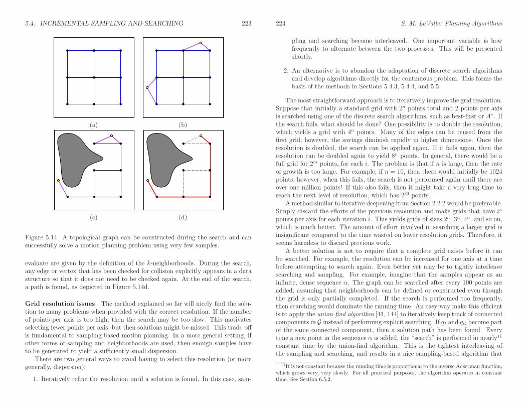
5.4. INCREMENTAL SAMPLING AND SEARCHING 223
(a) (b)
(c) (d)
Figure 5.14: A topological graph can be constructed during the search and cansuccessfully solve a motion planning problem using very few samples.
evaluate are given by the definition of the k-neighborhoods. During the search,any edge or vertex that has been checked for collision explicitly appears in a datastructure so that it does not need to be checked again. At the end of the search,a path is found, as depicted in Figure 5.14d.
Grid resolution issues The method explained so far will nicely find the solu-tion to many problems when provided with the correct resolution. If the numberof points per axis is too high, then the search may be too slow. This motivatesselecting fewer points per axis, but then solutions might be missed. This trade-offis fundamental to sampling-based motion planning. In a more general setting, ifother forms of sampling and neighborhoods are used, then enough samples haveto be generated to yield a sufficiently small dispersion.
There are two general ways to avoid having to select this resolution (or moregenerally, dispersion):
1. Iteratively refine the resolution until a solution is found. In this case, sam-
224 S. M. LaValle: Planning Algorithms
pling and searching become interleaved. One important variable is howfrequently to alternate between the two processes. This will be presentedshortly.
2. An alternative is to abandon the adaptation of discrete search algorithmsand develop algorithms directly for the continuous problem. This forms thebasis of the methods in Sections 5.4.3, 5.4.4, and 5.5.
The most straightforward approach is to iteratively improve the grid resolution.Suppose that initially a standard grid with 2n points total and 2 points per axisis searched using one of the discrete search algorithms, such as best-first or A∗. Ifthe search fails, what should be done? One possibility is to double the resolution,which yields a grid with 4n points. Many of the edges can be reused from thefirst grid; however, the savings diminish rapidly in higher dimensions. Once theresolution is doubled, the search can be applied again. If it fails again, then theresolution can be doubled again to yield 8n points. In general, there would be afull grid for 2ni points, for each i. The problem is that if n is large, then the rateof growth is too large. For example, if n = 10, then there would initially be 1024points; however, when this fails, the search is not performed again until there areover one million points! If this also fails, then it might take a very long time toreach the next level of resolution, which has 230 points.
A method similar to iterative deepening from Section 2.2.2 would be preferable.Simply discard the efforts of the previous resolution and make grids that have in
points per axis for each iteration i. This yields grids of sizes 2n, 3n, 4n, and so on,which is much better. The amount of effort involved in searching a larger grid isinsignificant compared to the time wasted on lower resolution grids. Therefore, itseems harmless to discard previous work.
A better solution is not to require that a complete grid exists before it canbe searched. For example, the resolution can be increased for one axis at a timebefore attempting to search again. Even better yet may be to tightly interleavesearching and sampling. For example, imagine that the samples appear as aninfinite, dense sequence α. The graph can be searched after every 100 points areadded, assuming that neighborhoods can be defined or constructed even thoughthe grid is only partially completed. If the search is performed too frequently,then searching would dominate the running time. An easy way make this efficientis to apply the union-find algorithm [41, 144] to iteratively keep track of connectedcomponents in G instead of performing explicit searching. If qI and qG become partof the same connected component, then a solution path has been found. Everytime a new point in the sequence α is added, the “search” is performed in nearly11
constant time by the union-find algorithm. This is the tightest interleaving ofthe sampling and searching, and results in a nice sampling-based algorithm that
11It is not constant because the running time is proportional to the inverse Ackerman function,which grows very, very slowly. For all practical purposes, the algorithm operates in constanttime. See Section 6.5.2.

5.4. INCREMENTAL SAMPLING AND SEARCHING 225
Random Walk BacktrackBest First
Stuck and i < K
Stuckand i=K
Reset i to 1
Increment i
Initialization (i=1)
Figure 5.15: The randomized potential field method can be modeled as a three-state machine.
requires no resolution parameter. It is perhaps best to select a sequence α thatcontains some lattice structure to facilitate the determination of neighborhoodsin each iteration.
What if we simply declare the resolution to be outrageously high at the outset?Imagine there are 100n points in the grid. This places all of the burden on thesearch algorithm. If the search algorithm itself is good at avoiding local minimaand has built-in multi-resolution qualities, then it may perform well without theiterative refinement of the sampling. The method of Section 5.4.3 is based onthis idea by performing best-first search on a high-resolution grid, combined withrandom walks to avoid local minima. The algorithms of Section 5.5 go one stepfurther and search in a multi-resolution way without requiring resolutions andneighborhoods to be explicitly determined. This can be considered as the limitingcase as the number of points per axis approaches infinity.
Although this section has focused on grids, it is also possible to use otherforms of sampling from Section 5.2. This requires defining the neighborhoodsin a suitable way that generalizes the k-neighborhoods of this section. In everycase, an infinite, dense sample sequence must be defined to obtain resolution com-pleteness by reducing the dispersion to zero in the limit. Methods for obtainingneighborhoods for irregular sample sets have been developed in the context ofsampling-based roadmaps; see Section 5.6. The notion of improving resolutionbecomes generalized to adding samples that improve dispersion (or even discrep-ancy).
5.4.3 Randomized Potential Fields
Adapting the discrete algorithms from Section 2.2 works well if the problem canbe solved with a small number of points. The number of points per axis mustbe small or the dimension must be low, to ensure that the number of points, kn,for k points per axis and n dimensions is small enough so that every vertex ing can be reached in a reasonable amount of time. If, for example, the problemrequires 50 points per axis and the dimension is 10, then it is impossible to searchall of the 5010 samples. Planners that exploit best-first heuristics might find theanswer without searching most of them; however, for a simple problem such as
226 S. M. LaValle: Planning Algorithms
that shown in Figure 5.13a, the planner will take too long exploring the verticesin the bowl.12
The randomized potential field [14, 16, 102] approach uses random walks toattempt to escape local minima when best-first search becomes stuck. It wasone of the first sampling-based planners that developed specialized techniquesbeyond classical discrete search, in an attempt to better solve challenging motionplanning problems. In many cases, remarkable results were obtained. In its time,the approach was able to solve problems up to 31 degrees of freedom, which waswell beyond what had been previously possible. The main drawback, however,was that the method involved many heuristic parameters that had to be adjustedfor each problem. This frustration eventually led to the development of betterapproaches, which are covered in Sections 5.4.4, 5.5, and 5.6. Nevertheless, it isworthwhile to study the clever heuristics involved in this earlier method becausethey illustrate many interesting issues, and the method was very influential in thedevelopment of other sampling-based planning algorithms.13
The most complicated part of the algorithm is the definition of a potentialfunction, which can be considered as a pseudometric that tries to estimate thedistance from any configuration to the goal. In most formulations, there is anattractive term, which is a metric on C that yields the distance to the goal, anda repulsive term, which penalizes configurations that come too close to obstacles.The construction of potential functions involves many heuristics and is coveredin great detail in [102]. One of the most effective methods involves constructingcost-to-go functions over W and lifting them to C [15]. In this section, it will besufficient to assume that some potential function, g(q), is defined, which is thesame notation (and notion) as a cost-to-go function in Section 2.2.2. In this case,however, there is no requirement that g(q) is optimal or even an underestimate ofthe true cost to go.
When the search becomes stuck and a random walk is needed, it is executed forsome number of iterations. Using the discretization procedures of Section 5.4.2, ahigh-resolution grid (e.g., 50 points per axis) is initially defined. In each iteration,the current configuration is modified as follows. Each coordinate, qi, is increasedor decreased by ∆qi (the grid step size) based on the outcome of a fair coin toss.Topological identifications must be respected, of course. After each iteration, thenew configuration is checked for collision, or whether it exceeds the boundary ofC (if it has a boundary). If so, then it is discarded, and another attempt is madefrom the previous configuration. The failures can repeat indefinitely until a newconfiguration in Cfree is obtained.
The resulting planner can be described in terms of a three-state machine,which is shown in Figure 5.15. Each state is called a mode to avoid confusion with
12Of course, that problem does not appear to need so many points per axis; fewer may beused instead, if the algorithm can adapt the sampling resolution or dispersion.
13The exciting results obtained by the method even helped inspire me many years ago to workon motion planning.

5.4. INCREMENTAL SAMPLING AND SEARCHING 227
earlier state-space concepts. The VSM and LPM are defined in terms of the mode.Initially, the planner is in the best first mode and uses qI to start a gradientdescent. While in the best first mode, the VSM selects the newest vertex,v ∈ V . In the first iteration, this is qI . The LPM creates a new vertex, vn, in aneighborhood of v, in a direction that minimizes g. The direction sampling maybe performed using randomly selected or deterministic samples. Using randomsamples, the sphere sampling method from Section 5.2.2 can be applied. Aftersome number of tries (another parameter), if the LPM is unsuccessful at reducingg, then the mode is changed to random walk because the best-first search isstuck in a local minimum of g.
In the random walk mode, a random walk is executed from the newestvertex. The random walk terminates if either g is lowered or a specified limitof iterations is reached. The limit is actually sampled from a predeterminedrandom variable (which contains parameters that also must be selected). Whenthe random walk mode terminates, the mode is changed back to best first. Acounter is incremented to keep track of the number of times that the random walkwas attempted. A parameter K determines the maximum number of attemptedrandom walks (a reasonable value is K = 20 [15]). If best first fails after Krandom walks have been attempted, then the backtrack mode is entered. Thebacktrack mode selects a vertex at random from among the vertices in V thatwere obtained during a random walk. Following this, the counter is reset, and themode is changed back to best first.
Due to the random walks, the resulting paths are often too complicated tobe useful in applications. Fortunately, it is straightforward to transform a com-puted path into a simpler one that is still collision-free. A common approach isto iteratively pick pairs of points at random along the domain of the path andattempt to replace the path segment with a straight-line path (in general, theshortest path in C). For example, suppose t1, t2 ∈ [0, 1] are chosen at random, andτ : [0, 1] → Cfree is the computed solution path. This path is transformed into anew path,
τ ′(t) =
τ(t) if 0 ≤ t ≤ t1aτ(t1) + (1− a)τ(t2) if t1 ≤ t ≤ t2τ(t) if t2 ≤ t ≤ 1,
(5.39)
in which a ∈ [0, 1] represents the fraction of the way from t1 to t2. Explicitly,a = (t2 − t)/(t2 − t1). The new path must be checked for collision. If it passes,then it replaces the old path; otherwise, it is discarded and a new pair t1, t2, ischosen.
The randomized potential field approach can escape high-dimensional localminima, which allow interesting solutions to be found for many challenging high-dimensional problems. Unfortunately, the heavy amount of parameter tuningcaused most people to abandon the method in recent times, in favor of newermethods.
228 S. M. LaValle: Planning Algorithms
5.4.4 Other Methods
Several influential sampling-based methods are given here. Each of them appearsto offer advantages over the randomized potential field method. All of them userandomization, which was perhaps inspired by the potential field method.
Ariadne’s Clew algorithm This approach grows a search tree that is biasedto explore as much new territory as possible in each iteration [129, 128]. There aretwo modes, search and explore, which alternate over successive iterations. Inthe explore mode, the VSM selects a vertex, ve, at random, and the LPM findsa new configuration that can be easily connected to ve and is as far as possiblefrom the other vertices in G. A global optimization function that aggregates thedistances to other vertices is optimized using a genetic algorithm. In the searchmode, an attempt is made to extend the vertex added in the explore mode tothe goal configuration. The key idea from this approach, which influenced boththe next approach and the methods in Section 5.5, is that some of the time mustbe spent exploring the space, as opposed to focusing on finding the solution. Thegreedy behavior of the randomized potential field led to some efficiency but wasalso its downfall for some problems because it was all based on escaping localminima with respect to the goal instead of investing time on global exploration.One disadvantage of Ariadne’s Clew algorithm is that it is very difficult to solvethe optimization problem for placing a new vertex in the explore mode. Geneticalgorithms were used in [128], which are generally avoided for motion planningbecause of the required problem-specific parameter tuning.
Expansive-space planner This method [79, 148] generates samples in a waythat attempts to explore new parts of the space. In this sense, it is similar tothe explore mode of the Ariadne’s Clew algorithm. Furthermore, the planneris made more efficient by borrowing the bidirectional search idea from discretesearch algorithms, as covered in Section 2.2.3. The VSM selects a vertex, ve,from G with a probability that is inversely proportional to the number of othervertices of G that lie within a predetermined neighborhood of ve. Thus, “isolated”vertices are more likely to be chosen. The LPM generates a new vertex vn atrandom within a predetermined neighborhood of ve. It will decide to insert vninto G with a probability that is inversely proportional to the number of othervertices of G that lie within a predetermined neighborhood of vn. For a fixednumber of iterations, the VSM repeatedly chooses the same vertex, until movingon to another vertex. The resulting planner is able to solve many interestingproblems by using a surprisingly simple criterion for the placement of points. Themain drawbacks are that the planner requires substantial parameter tuning, whichis problem-specific (or at least specific to a similar family of problems), and theperformance tends to degrade if the query requires systematically searching a longlabyrinth. Choosing the radius of the predetermined neighborhoods essentiallyamounts to determining the appropriate resolution.

5.5. RAPIDLY EXPLORING DENSE TREES 229
Random-walk planner A surprisingly simple and efficient algorithm can bemade entirely from random walks [31]. To avoid parameter tuning, the algorithmadjusts its distribution of directions and magnitude in each iteration, based on thesuccess of the past k iterations (perhaps k is the only parameter). In each iteration,the VSM just selects the vertex that was most recently added to G. The LPMgenerates a direction and magnitude by generating samples from a multivariateGaussian distribution whose covariance parameters are adaptively tuned. Themain drawback of the method is similar to that of the previous method. Bothhave difficulty traveling through long, winding corridors. It is possible to combineadaptive random walks with other search algorithms, such as the potential fieldplanner [30].
5.5 Rapidly Exploring Dense Trees
This section introduces an incremental sampling and searching approach thatyields good performance in practice without any parameter tuning.14 The ideais to incrementally construct a search tree that gradually improves the resolutionbut does not need to explicitly set any resolution parameters. In the limit, the treedensely covers the space. Thus, it has properties similar to space filling curves[147], but instead of one long path, there are shorter paths that are organizedinto a tree. A dense sequence of samples is used as a guide in the incrementalconstruction of the tree. If this sequence is random, the resulting tree is calleda rapidly exploring random tree (RRT). In general, this family of trees, whetherthe sequence is random or deterministic, will be referred to as rapidly exploringdense trees (RDTs) to indicate that a dense covering of the space is obtained. Thismethod was originally developed for motion planning under differential constraints[105, 108]; that case is covered in Section 14.4.3.
5.5.1 The Exploration Algorithm
Before explaining how to use these trees to solve a planning query, imagine thatthe goal is to get as close as possible to every configuration, starting from aninitial configuration. The method works for any dense sequence. Once again, letα denote an infinite, dense sequence of samples in C. The ith sample is denotedby α(i). This may possibly include a uniform, random sequence, which is onlydense with probability one. Random sequences that induce a nonuniform bias arealso acceptable, as long as they are dense with probability one.
An RDT is a topological graph, G(V,E). Let S ⊂ Cfree indicate the set of allpoints reached by G. Since each e ∈ E is a path, this can be expressed as the
14The original RRT [103] was introduced with a step size parameter, but this is eliminated inthe current presentation. For implementation purposes, one might still want to revert to thisolder way of formulating the algorithm because the implementation is a little easier. This willbe discussed shortly.
230 S. M. LaValle: Planning Algorithms
SIMPLE RDT(q0)1 G.init(q0);2 for i = 1 to k do3 G.add vertex(α(i));4 qn ← nearest(S(G), α(i));5 G.add edge(qn, α(i));
Figure 5.16: The basic algorithm for constructing RDTs (which includes RRTsas a special case) when there are no obstacles. It requires the availability of adense sequence, α, and iteratively connects from α(i) to the nearest point amongall those reached by G.
q0
qn
α(i)
q0
(a) (b)
Figure 5.17: (a) Suppose inductively that this tree has been constructed so farusing the algorithm in Figure 5.16. (b) A new edge is added that connects fromthe sample α(i) to the nearest point in S, which is the vertex qn.
swath, S, of the graph, which is defined as
S =⋃
e∈E
e([0, 1]). (5.40)
In (5.40), e([0, 1]) ⊆ Cfree is the image of the path e.The exploration algorithm is first explained in Figure 5.16 without any obsta-
cles or boundary obstructions. It is assumed that C is a metric space. Initially, avertex is made at q0. For k iterations, a tree is iteratively grown by connectingα(i) to its nearest point in the swath, S. The connection is usually made along
qn
α(i)q0
Figure 5.18: If the nearest point in S lies in an edge, then the edge is split intotwo, and a new vertex is inserted into G.
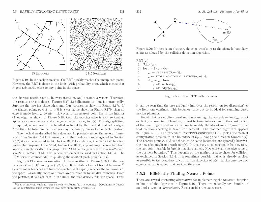
5.5. RAPIDLY EXPLORING DENSE TREES 231
45 iterations 2345 iterations
Figure 5.19: In the early iterations, the RRT quickly reaches the unexplored parts.However, the RRT is dense in the limit (with probability one), which means thatit gets arbitrarily close to any point in the space.
the shortest possible path. In every iteration, α(i) becomes a vertex. Therefore,the resulting tree is dense. Figures 5.17–5.18 illustrate an iteration graphically.Suppose the tree has three edges and four vertices, as shown in Figure 5.17a. Ifthe nearest point, qn ∈ S, to α(i) is a vertex, as shown in Figure 5.17b, then anedge is made from qn to α(i). However, if the nearest point lies in the interiorof an edge, as shown in Figure 5.18, then the existing edge is split so that qnappears as a new vertex, and an edge is made from qn to α(i). The edge splitting,if required, is assumed to be handled in line 4 by the method that adds edges.Note that the total number of edges may increase by one or two in each iteration.
The method as described here does not fit precisely under the general frame-work from Section 5.4.1; however, with the modifications suggested in Section5.5.2, it can be adapted to fit. In the RDT formulation, the nearest functionserves the purpose of the VSM, but in the RDT, a point may be selected fromanywhere in the swath of the graph. The VSM can be generalized to a swath-pointselection method, SSM. This generalization will be used in Section 14.3.4. TheLPM tries to connect α(i) to qn along the shortest path possible in C.
Figure 5.19 shows an execution of the algorithm in Figure 5.16 for the casein which C = [0, 1]2 and q0 = (1/2, 1/2). It exhibits a kind of fractal behavior.15
Several main branches are first constructed as it rapidly reaches the far corners ofthe space. Gradually, more and more area is filled in by smaller branches. Fromthe pictures, it is clear that in the limit, the tree densely fills the space. Thus,
15If α is uniform, random, then a stochastic fractal [101] is obtained. Deterministic fractalscan be constructed using sequences that have appropriate symmetries.
232 S. M. LaValle: Planning Algorithms
qn
q0
Cobs
qs
α(i)
Figure 5.20: If there is an obstacle, the edge travels up to the obstacle boundary,as far as allowed by the collision detection algorithm.
RDT(q0)1 G.init(q0);2 for i = 1 to k do3 qn ← nearest(S, α(i));4 qs ← stopping-configuration(qn,α(i));5 if qs 6= qn then6 G.add vertex(qs);7 G.add edge(qn, qs);
Figure 5.21: The RDT with obstacles.
it can be seen that the tree gradually improves the resolution (or dispersion) asthe iterations continue. This behavior turns out to be ideal for sampling-basedmotion planning.
Recall that in sampling-based motion planning, the obstacle region Cobs is notexplicitly represented. Therefore, it must be taken into account in the constructionof the tree. Figure 5.20 indicates how to modify the algorithm in Figure 5.16 sothat collision checking is taken into account. The modified algorithm appearsin Figure 5.21. The procedure stopping-configuration yields the nearestconfiguration possible to the boundary of Cfree, along the direction toward α(i).The nearest point qn ∈ S is defined to be same (obstacles are ignored); however,the new edge might not reach to α(i). In this case, an edge is made from qn to qs,the last point possible before hitting the obstacle. How close can the edge come tothe obstacle boundary? This depends on the method used to check for collision,as explained in Section 5.3.4. It is sometimes possible that qn is already as closeas possible to the boundary of Cfree in the direction of α(i). In this case, no newedge or vertex is added that for that iteration.
5.5.2 Efficiently Finding Nearest Points
There are several interesting alternatives for implementing the nearest functionin line 3 of the algorithm in Figure 5.16. There are generally two families ofmethods: exact or approximate. First consider the exact case.

5.5. RAPIDLY EXPLORING DENSE TREES 233
Exact solutions Suppose that all edges in G are line segments in Rm for somedimension m ≥ n. An edge that is generated early in the construction process willbe split many times in later iterations. For the purposes of finding the nearestpoint in S, however, it is best to handle this as a single segment. For example, seethe three large branches that extend from the root in Figure 5.19. As the numberof points increases, the benefit of agglomerating the segments increases. Let eachof these agglomerated segments be referred to as a supersegment. To implementnearest, a primitive is needed that computes the distance between a point and aline segment. This can be performed in constant time with simple vector calculus.Using this primitive, nearest is implemented by iterating over all supersegmentsand taking the point with minimum distance among all of them. It may be possibleto improve performance by building hierarchical data structures that can eliminatelarge sets of supersegments, but this remains to be seen experimentally.
In some cases, the edges of G may not be line segments. For example, the short-est paths between two points in SO(3) are actually circular arcs along S3. Onepossible solution is to maintain a separate parameterization of C for the purposesof computing the nearest function. For example, SO(3) can be represented as[0, 1]3/ ∼, by making the appropriate identifications to obtain RP3. Straight-linesegments can then be used. The problem is that the resulting metric is not con-sistent with the Haar measure, which means that an accidental bias would result.Another option is to tightly enclose S3 in a 4D cube. Every point on S3 can bemapped outward onto a cube face. Due to antipodal identification, only four ofthe eight cube faces need to be used to obtain a bijection between the set of allrotation and the cube surface. Linear interpolation can be used along the cubefaces, as long as both points remain on the same face. If the points are on differentfaces, then two line segments can be used by bending the shortest path aroundthe corner between the two faces. This scheme will result in less distortion thanmapping SO(3) to [0, 1]3/ ∼; however, some distortion will still exist.
Another approach is to avoid distortion altogether and implement primitivesthat can compute the distance between a point and a curve. In the case of SO(3),a primitive is needed that can find the distance between a circular arc in Rm
and a point in Rm. This might not be too difficult, but if the curves are morecomplicated, then an exact implementation of the nearest function may be tooexpensive computationally.
Approximate solutions Approximate solutions are much easier to construct,however, a resolution parameter is introduced. Each path segment can be approx-imated by inserting intermediate vertices along long segments, as shown in Figure5.22. The intermediate vertices should be added each time a new sample, α(i),is inserted into G. A parameter ∆q can be defined, and intermediate samples areinserted to ensure that no two consecutive vertices in G are ever further than ∆qfrom each other. Using intermediate vertices, the interiors of the edges in G areignored when finding the nearest point in S. The approximate computation of
234 S. M. LaValle: Planning Algorithms
qn
q0 α(i)
Figure 5.22: For implementation ease, intermediate vertices can be inserted toavoid checking for closest points along line segments. The trade-off is that thenumber of vertices is increased dramatically.
13
12
14
118
910
7
4
5
6
2 3
1
7
8
3 1 10 11
2 4 6 9 13 14
12
5
Figure 5.23: A Kd-tree can be used for efficient nearest-neighbor computations.
nearest is performed by finding the closest vertex to α(i) in G. This approachis by far the simplest to implement. It also fits precisely under the incrementalsampling and searching framework from Section 5.4.1.
When using intermediate vertices, the trade-offs are clear. The computationtime for each evaluation of nearest is linear in the number of vertices. Increasingthe number of vertices improves the quality of the approximation, but it alsodramatically increases the running time. One way to recover some of this cost isto insert the vertices into an efficient data structure for nearest-neighbor searching.One of the most practical and widely used data structures is the Kd-tree [46, 58,137]. A depiction is shown in Figure 5.23 for 14 points in R2. The Kd-tree canbe considered as a multi-dimensional generalization of a binary search tree. TheKd-tree is constructed for points, P , in R2 as follows. Initially, sort the pointswith respect to the x coordinate. Take the median point, p ∈ P , and divideP into two sets, depending on which side of a vertical line through p the otherpoints fall. For each of the two sides, sort the points by the y coordinate and findtheir medians. Points are divided at this level based on whether they are aboveor below horizontal lines. At the next level of recursion, vertical lines are usedagain, followed by horizontal again, and so on. The same idea can be applied inRn by cycling through the n coordinates, instead of alternating between x and y,to form the divisions. In [9], the Kd-tree is extended to topological spaces thatarise in motion planning and is shown to yield good performance for RRTs andsampling-based roadmaps. A Kd-tree of k points can be constructed in O(nk lg k)time. Topological identifications must be carefully considered when traversing
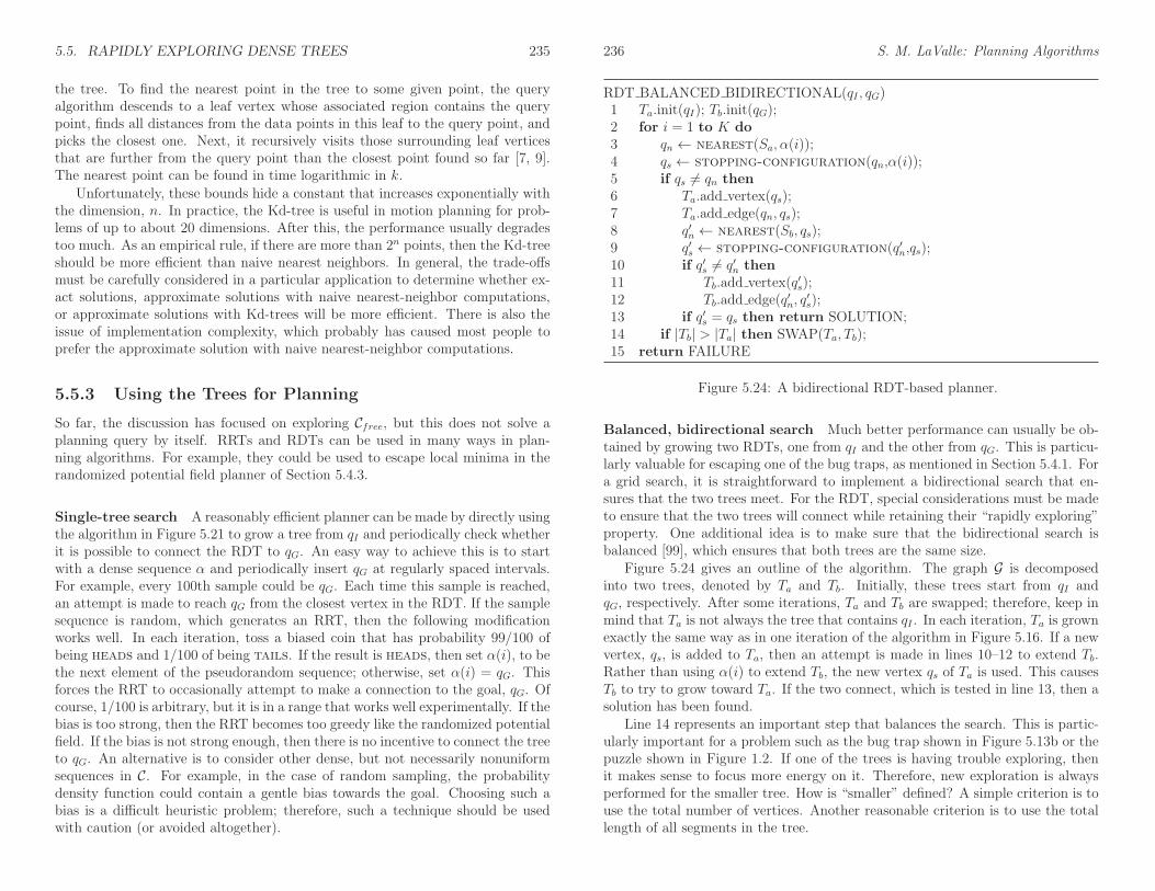
5.5. RAPIDLY EXPLORING DENSE TREES 235
the tree. To find the nearest point in the tree to some given point, the queryalgorithm descends to a leaf vertex whose associated region contains the querypoint, finds all distances from the data points in this leaf to the query point, andpicks the closest one. Next, it recursively visits those surrounding leaf verticesthat are further from the query point than the closest point found so far [7, 9].The nearest point can be found in time logarithmic in k.
Unfortunately, these bounds hide a constant that increases exponentially withthe dimension, n. In practice, the Kd-tree is useful in motion planning for prob-lems of up to about 20 dimensions. After this, the performance usually degradestoo much. As an empirical rule, if there are more than 2n points, then the Kd-treeshould be more efficient than naive nearest neighbors. In general, the trade-offsmust be carefully considered in a particular application to determine whether ex-act solutions, approximate solutions with naive nearest-neighbor computations,or approximate solutions with Kd-trees will be more efficient. There is also theissue of implementation complexity, which probably has caused most people toprefer the approximate solution with naive nearest-neighbor computations.
5.5.3 Using the Trees for Planning
So far, the discussion has focused on exploring Cfree, but this does not solve aplanning query by itself. RRTs and RDTs can be used in many ways in plan-ning algorithms. For example, they could be used to escape local minima in therandomized potential field planner of Section 5.4.3.
Single-tree search A reasonably efficient planner can be made by directly usingthe algorithm in Figure 5.21 to grow a tree from qI and periodically check whetherit is possible to connect the RDT to qG. An easy way to achieve this is to startwith a dense sequence α and periodically insert qG at regularly spaced intervals.For example, every 100th sample could be qG. Each time this sample is reached,an attempt is made to reach qG from the closest vertex in the RDT. If the samplesequence is random, which generates an RRT, then the following modificationworks well. In each iteration, toss a biased coin that has probability 99/100 ofbeing heads and 1/100 of being tails. If the result is heads, then set α(i), to bethe next element of the pseudorandom sequence; otherwise, set α(i) = qG. Thisforces the RRT to occasionally attempt to make a connection to the goal, qG. Ofcourse, 1/100 is arbitrary, but it is in a range that works well experimentally. If thebias is too strong, then the RRT becomes too greedy like the randomized potentialfield. If the bias is not strong enough, then there is no incentive to connect the treeto qG. An alternative is to consider other dense, but not necessarily nonuniformsequences in C. For example, in the case of random sampling, the probabilitydensity function could contain a gentle bias towards the goal. Choosing such abias is a difficult heuristic problem; therefore, such a technique should be usedwith caution (or avoided altogether).
236 S. M. LaValle: Planning Algorithms
RDT BALANCED BIDIRECTIONAL(qI , qG)1 Ta.init(qI); Tb.init(qG);2 for i = 1 to K do3 qn ← nearest(Sa, α(i));4 qs ← stopping-configuration(qn,α(i));5 if qs 6= qn then6 Ta.add vertex(qs);7 Ta.add edge(qn, qs);8 q′n ← nearest(Sb, qs);9 q′s ← stopping-configuration(q′n,qs);10 if q′s 6= q′n then11 Tb.add vertex(q′s);12 Tb.add edge(q′n, q
′s);
13 if q′s = qs then return SOLUTION;14 if |Tb| > |Ta| then SWAP(Ta, Tb);15 return FAILURE
Figure 5.24: A bidirectional RDT-based planner.
Balanced, bidirectional search Much better performance can usually be ob-tained by growing two RDTs, one from qI and the other from qG. This is particu-larly valuable for escaping one of the bug traps, as mentioned in Section 5.4.1. Fora grid search, it is straightforward to implement a bidirectional search that en-sures that the two trees meet. For the RDT, special considerations must be madeto ensure that the two trees will connect while retaining their “rapidly exploring”property. One additional idea is to make sure that the bidirectional search isbalanced [99], which ensures that both trees are the same size.
Figure 5.24 gives an outline of the algorithm. The graph G is decomposedinto two trees, denoted by Ta and Tb. Initially, these trees start from qI andqG, respectively. After some iterations, Ta and Tb are swapped; therefore, keep inmind that Ta is not always the tree that contains qI . In each iteration, Ta is grownexactly the same way as in one iteration of the algorithm in Figure 5.16. If a newvertex, qs, is added to Ta, then an attempt is made in lines 10–12 to extend Tb.Rather than using α(i) to extend Tb, the new vertex qs of Ta is used. This causesTb to try to grow toward Ta. If the two connect, which is tested in line 13, then asolution has been found.
Line 14 represents an important step that balances the search. This is partic-ularly important for a problem such as the bug trap shown in Figure 5.13b or thepuzzle shown in Figure 1.2. If one of the trees is having trouble exploring, thenit makes sense to focus more energy on it. Therefore, new exploration is alwaysperformed for the smaller tree. How is “smaller” defined? A simple criterion is touse the total number of vertices. Another reasonable criterion is to use the totallength of all segments in the tree.

5.6. ROADMAP METHODS FOR MULTIPLE QUERIES 237
An unbalanced bidirectional search can instead be made by forcing the treesto be swapped in every iteration. Once the trees are swapped, then the roles arereversed. For example, after the first swap, Tb is extended in the same way asan integration in Figure 5.16, and if a new vertex qs is added then an attempt ismade to connect Ta to qs.
One important concern exists when α is deterministic. It might be possiblethat even though α is dense, when the samples are divided among the trees, eachmay not receive a dense set. If each uses its own deterministic sequence, then thisproblem can be avoided. In the case of making a bidirectional RRT planner, thesame (pseudo)random sequence can be used for each tree without encounteringsuch troubles.
More than two trees If a dual-tree approach offers advantages over a singletree, then it is natural to ask whether growing three or more RDTs might beeven better. This is particularly helpful for problems like the double bug trap inFigure 5.13c. New trees can be grown from parts of C that are difficult to reach.Controlling the number of trees and determining when to attempt connectionsbetween them is difficult. Some interesting recent work has been done in thisdirection [18, 156, 157].
These additional trees could be started at arbitrary (possibly random) configu-rations. As more trees are considered, a complicated decision problem arises. Thecomputation time must be divided between attempting to explore the space andattempting to connect trees to each other. It is also not clear which connectionsshould be attempted. Many research issues remain in the development of this andother RRT-based planners. A limiting case would be to start a new tree fromevery sample in α(i) and to try to connect nearby trees whenever possible. Thisapproach results in a graph that covers the space in a nice way that is independentof the query. This leads to the main topic of the next section.
5.6 Roadmap Methods for Multiple Queries
Previously, it was assumed that a single initial-goal pair was given to the planningalgorithm. Suppose now that numerous initial-goal queries will be given to thealgorithm, while keeping the robot model and obstacles fixed. This leads to amultiple-query version of the motion planning problem. In this case, it makessense to invest substantial time to preprocess the models so that future queriescan be answered efficiently. The goal is to construct a topological graph calleda roadmap, which efficiently solves multiple initial-goal queries. Intuitively, thepaths on the roadmap should be easy to reach from each of qI and qG, and thegraph can be quickly searched for a solution. The general framework presentedhere was mainly introduced in [90] under the name probabilistic roadmaps (PRMs).The probabilistic aspect, however, is not important to the method. Therefore, we
238 S. M. LaValle: Planning Algorithms
BUILD ROADMAP1 G.init(); i← 0;2 while i < N3 if α(i) ∈ Cfree then4 G.add vertex(α(i)); i← i+ 1;5 for each q ∈ neighborhood(α(i),G)6 if ((not G.same component(α(i), q)) and connect(α(i), q)) then7 G.add edge(α(i), q);
Figure 5.25: The basic construction algorithm for sampling-based roadmaps. Notethat i is not incremented if α(i) is in collision. This forces i to correctly count thenumber of vertices in the roadmap.
call this family of methods sampling-based roadmaps. This distinguishes themfrom combinatorial roadmaps, which will appear in Chapter 6.
5.6.1 The Basic Method
Once again, let G(V,E) represent a topological graph in which V is a set of verticesand E is the set of paths that map into Cfree. Under the multiple-query philosophy,motion planning is divided into two phases of computation:
Preprocessing Phase: During the preprocessing phase, substantial effortis invested to build G in a way that is useful for quickly answering futurequeries. For this reason, it is called a roadmap, which in some sense shouldbe accessible from every part of Cfree.
Query Phase: During the query phase, a pair, qI and qG, is given. Eachconfiguration must be connected easily to G using a local planner. Followingthis, a discrete search is performed using any of the algorithms in Section2.2 to obtain a sequence of edges that forms a path from qI to qG.
Generic preprocessing phase Figure 5.25 presents an outline of the basicpreprocessing phase, and Figure 5.26 illustrates the algorithm. As seen throughoutthis chapter, the algorithm utilizes a uniform, dense sequence α. In each iteration,the algorithm must check whether α(i) ∈ Cfree. If α(i) ∈ Cobs, then it mustcontinue to iterate until a collision-free sample is obtained. Once α(i) ∈ Cfree,then in line 4 it is inserted as a vertex of G. The next step is to try to connect α(i)to some nearby vertices, q, of G. Each connection is attempted by the connect
function, which is a typical LPM (local planning method) from Section 5.4.1.In most implementations, this simply tests the shortest path between α(i) andq. Experimentally, it seems most efficient to use the multi-resolution, van derCorput–based method described at the end of Section 5.3.4 [59]. Instead of theshortest path, it is possible to use more sophisticated connection methods, such

5.6. ROADMAP METHODS FOR MULTIPLE QUERIES 239
α(i)
Cobs
Cobs
Figure 5.26: The sampling-based roadmap is constructed incrementally by at-tempting to connect each new sample, α(i), to nearby vertices in the roadmap.
as the bidirectional algorithm in Figure 5.24. If the path is collision-free, thenconnect returns true.
The same component condition in line 6 checks to make sure α(i) and q are indifferent components of G before wasting time on collision checking. This ensuresthat every time a connection is made, the number of connected components of G isdecreased. This can be implemented very efficiently (near constant time) using thepreviously mentioned union-find algorithm [41, 144]. In some implementations thisstep may be ignored, especially if it is important to generate multiple, alternativesolutions. For example, it may be desirable to generate solution paths from differ-ent homotopy classes. In this case the condition (not G.same component(α(i), q))is replaced with G.vertex degree(q) < K, for some fixed K (e.g., K = 15).
Selecting neighboring samples Several possible implementations of line 5 canbe made. In all of these, it seems best to sort the vertices that will be consideredfor connection in order of increasing distance from α(i). This makes sense becauseshorter paths are usually less costly to check for collision, and they also have ahigher likelihood of being collision-free. If a connection is made, this avoids costlycollision checking of longer paths to configurations that would eventually belongto the same connected component.
Several useful implementations of neighborhood are
1. Nearest K: The K closest points to α(i) are considered. This requiressetting the parameter K (a typical value is 15). If you are unsure whichimplementation to use, try this one.
2. Component K: Try to obtain up to K nearest samples from each con-nected component of G. A reasonable value is K = 1; otherwise, too manyconnections would be tried.
3. Radius: Take all points within a ball of radius r centered at α(i). Anupper limit, K, may be set to prevent too many connections from being
240 S. M. LaValle: Planning Algorithms
attempted. Typically, K = 20. A radius can be determined adaptively byshrinking the ball as the number of points increases. This reduction canbe based on dispersion or discrepancy, if either of these is available for α.Note that if the samples are highly regular (e.g., a grid), then choosing thenearest K and taking points within a ball become essentially equivalent.If the point set is highly irregular, as in the case of random samples, thentaking the nearest K seems preferable.
4. Visibility: In Section 5.6.2, a variant will be described for which it isworthwhile to try connecting α to all vertices in G.
Note that all of these require C to be a metric space. One variation that has not yetbeen given much attention is to ensure that the directions of the neighborhoodpoints relative to α(i) are distributed uniformly. For example, if the 20 closestpoints are all clumped together in the same direction, then it may be preferableto try connecting to a further point because it is in the opposite direction.
Query phase In the query phase, it is assumed that G is sufficiently completeto answer many queries, each of which gives an initial configuration, qI , and a goalconfiguration, qG. First, the query phase pretends as if qI and qG were chosen fromα for connection to G. This requires running two more iterations of the algorithmin Figure 5.25. If qI and qG are successfully connected to other vertices in G, thena search is performed for a path that connects the vertex qI to the vertex qG. Thepath in the graph corresponds directly to a path in Cfree, which is a solution to thequery. Unfortunately, if this method fails, it cannot be determined conclusivelywhether a solution exists. If the dispersion is known for a sample sequence, α,then it is at least possible to conclude that no solution exists for the resolution ofthe planner. In other words, if a solution does exist, it would require the path totravel through a corridor no wider than the radius of the largest empty ball [104].
Some analysis There have been many works that analyze the performance ofsampling-based roadmaps. The basic idea from one of them [13] is briefly pre-sented here. Consider problems such as the one in Figure 5.27, in which the con-nect method will mostly likely fail in the thin tube, even though a connectionexists. The higher dimensional versions of these problems are even more difficult.Many planning problems involve moving a robot through an area with tight clear-ance. This generally causes narrow channels to form in Cfree, which leads to achallenging planning problem for the sampling-based roadmap algorithm. Findingthe escape of a bug trap is also challenging, but for the roadmap methods, eventraveling through a single corridor is hard (unless more sophisticated LPMs areused [83]).
Let V (q) denote the set of all configurations that can be connected to q usingthe connectmethod. Intuitively, this is considered as the set of all configurationsthat can be “seen” using line-of-sight visibility, as shown in Figure 5.28a

5.6. ROADMAP METHODS FOR MULTIPLE QUERIES 241
qGqI
Figure 5.27: An example such as this is difficult for sampling-based roadmaps (inhigher dimensional C-spaces) because some samples must fall along many pointsin the curved tube. Other methods, however, may be able to easily solve it.
V (q)
q
(a) Visibility definition (b) Visibility roadmap
Figure 5.28: (a) V (q) is the set of points reachable by the LPM from q. (b) Avisibility roadmap has two kinds of vertices: guards, which are shown in black,and connectors, shown in white. Guards are not allowed to see other guards.Connectors must see at least two guards.
242 S. M. LaValle: Planning Algorithms
The ǫ-goodness of Cfree is defined as
ǫ(Cfree) = minq∈Cfree
{
µ(V (q))
µ(Cfree)
}
, (5.41)
in which µ represents the measure. Intuitively, ǫ(Cfree) represents the small frac-tion of Cfree that is visible from any point. In terms of ǫ and the number of verticesin G, bounds can be established that yield the probability that a solution will befound [13]. The main difficulties are that the ǫ-goodness concept is very conserva-tive (it uses worst-case analysis over all configurations), and ǫ-goodness is definedin terms of the structure of Cfree, which cannot be computed efficiently. Thisresult and other related results help to gain a better understanding of sampling-based planning, but such bounds are difficult to apply to particular problems todetermine whether an algorithm will perform well.
5.6.2 Visibility Roadmap
One of the most useful variations of sampling-based roadmaps is the visibilityroadmap [152]. The approach works very hard to ensure that the roadmap rep-resentation is small yet covers Cfree well. The running time is often greater thanthe basic algorithm in Figure 5.25, but the extra expense is usually worthwhile ifthe multiple-query philosophy is followed to its fullest extent.
The idea is to define two different kinds of vertices in G:
Guards: To become a guard, a vertex, q must not be able to see otherguards. Thus, the visibility region, V (q), must be empty of other guards.
Connectors: To become a connector, a vertex, q, must see at least twoguards. Thus, there exist guards q1 and q2, such that q ∈ V (q1) ∩ V (q2).
The roadmap construction phase proceeds similarly to the algorithm in Figure5.25. The neighborhood function returns all vertices in G. Therefore, for each newsample α(i), an attempt is made to connect it to every other vertex in G.
The main novelty of the visibility roadmap is using a strong criterion to deter-mine whether to keep α(i) and its associated edges in G. There are three possiblecases for each α(i):
1. The new sample, α(i), is not able to connect to any guards. In this case,α(i) earns the privilege of becoming a guard itself and is inserted into G.
2. The new sample can connect to guards from at least two different connectedcomponents of G. In this case, it becomes a connector that is inserted intoG along with its associated edges, which connect it to these guards fromdifferent components.

5.6. ROADMAP METHODS FOR MULTIPLE QUERIES 243
3. Neither of the previous two conditions were satisfied. This means that thesample could only connect to guards in the same connected component. Inthis case, α(i) is discarded.
The final condition causes a dramatic reduction in the number of roadmap vertices.One problem with this method is that it does not allow guards to be deleted in
favor of better guards that might appear later. The placement of guards dependsstrongly on the order in which samples appear in α. The method may performpoorly if guards are not positioned well early in the sequence. It would be betterto have an adaptive scheme in which guards could be reassigned in later iterationsas better positions become available. Accomplishing this efficiently remains anopen problem. Note the algorithm is still probabilistically complete using randomsampling or resolution complete if α is dense, even though many samples arerejected.
5.6.3 Heuristics for Improving Roadmaps
The quest to design a good roadmap through sampling has spawned many heuris-tic approaches to sampling and making connections in roadmaps. Most of theseexploit properties that are specific to the shape of the C-space and/or the partic-ular geometry and kinematics of the robot and obstacles. The emphasis is usuallyon finding ways to dramatically reduce the number or required samples. Severalof these methods are briefly described here.
Vertex enhancement [90] This heuristic strategy focuses effort on verticesthat were difficult to connect to other vertices in the roadmap construction algo-rithm in Figure 5.25. A probability distribution, P (v), is defined over the verticesv ∈ V . A number of iterations are then performed in which a vertex is sampledfrom V according to P (v), and then some random motions are performed from vto try to reach new configurations. These new configurations are added as ver-tices, and attempts are made to connect them to other vertices, as selected bythe neighborhood function in an ordinary iteration of the algorithm in Figure5.25. A recommended heuristic [90] for defining P (v) is to define a statistic foreach v as nf/(nt + 1), in which nt is the total number of connections attemptedfor v, and nf is the number of times these attempts failed. The probability P (v)is assigned as nf/(nt +1)m, in which m is the sum of the statistics over all v ∈ V(this normalizes the statistics to obtain a valid probability distribution).
Sampling on the Cfree boundary [3, 5] This scheme is based on the intuitionthat it is sometimes better to sample along the boundary, ∂Cfree, rather thanwaste samples on large areas of Cfree that might be free of obstacles. Figure 5.29ashows one way in which this can be implemented. For each sample of α(i) thatfalls into Cobs, a number of random directions are chosen in C; these directions canbe sampled using the Sn sampling method from Section 5.2.2. For each direction,
244 S. M. LaValle: Planning Algorithms
1α(i)
Cobs
4
23
Cobs Cobs
(a) (b)
Figure 5.29: (a) To obtain samples along the boundary, binary search is usedalong random directions from a sample in Cobs. (b) The bridge test finds narrowcorridors by examining a triple of nearby samples along a line.
a binary search is performed to get a sample in Cfree that is as close as possibleto Cobs. The order of point evaluation in the binary search is shown in Figure5.29a. Let τ : [0, 1] denote the path for which τ(0) ∈ Cobs and τ(1) ∈ Cfree. In thefirst step, test the midpoint, τ(1/2). If τ(1/2) ∈ Cfree, this means that ∂Cfree liesbetween τ(0) and τ(1/2); otherwise, it lies between τ(1/2) and τ(1). The nextiteration selects the midpoint of the path segment that contains ∂Cfree. This willbe either τ(1/4) or τ(3/4). The process continues recursively until the desiredresolution is obtained.
Gaussian sampling [23] The Gaussian sampling strategy follows some of thesame motivation for sampling on the boundary. In this case, the goal is to obtainpoints near ∂Cfree by using a Gaussian distribution that biases the samples to becloser to ∂Cfree, but the bias is gentler, as prescribed by the variance parameterof the Gaussian. The samples are generated as follows. Generate one sample,q1 ∈ C, uniformly at random. Following this, generate another sample, q2 ∈ C,according to a Gaussian with mean q1; the distribution must be adapted for anytopological identifications and/or boundaries of C. If one of q1 or q2 lies in Cfreeand the other lies in Cobs, then the one that lies in Cfree is kept as a vertex in theroadmap. For some examples, this dramatically prunes the number of requiredvertices.
Bridge-test sampling [78] The Gaussian sampling strategy decides to keep apoint based in part on testing a pair of samples. This idea can be carried one stepfurther to obtain a bridge test, which uses three samples along a line segment.If the samples are arranged as shown in Figure 5.29b, then the middle samplebecomes a roadmap vertex. This is based on the intuition that narrow corridorsare thin in at least one direction. The bridge test indicates that a point lies in athin corridor, which is often an important place to locate a vertex.
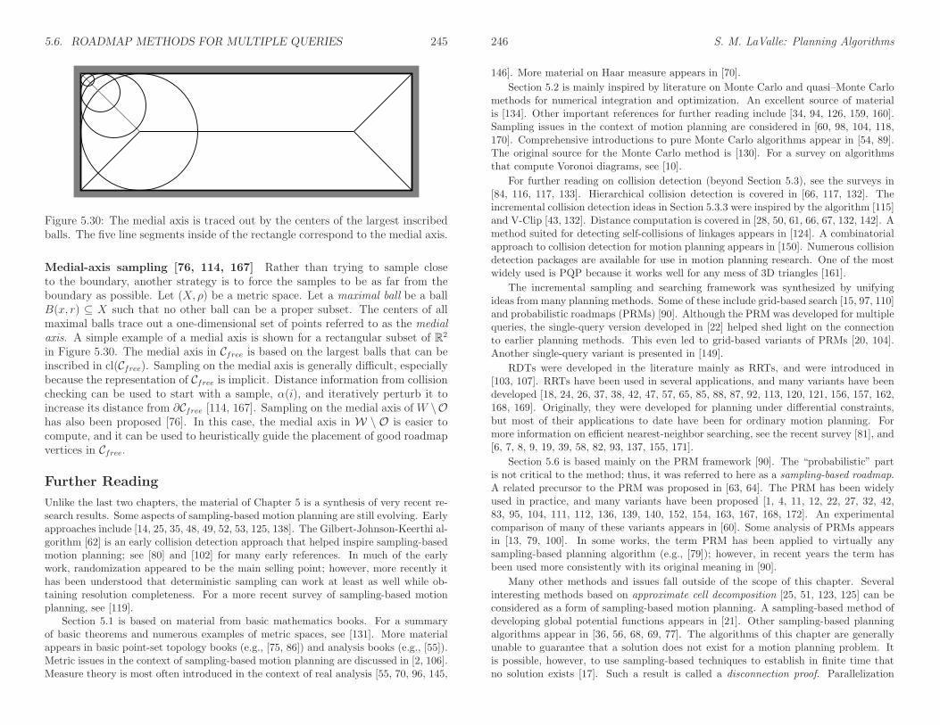
5.6. ROADMAP METHODS FOR MULTIPLE QUERIES 245
Figure 5.30: The medial axis is traced out by the centers of the largest inscribedballs. The five line segments inside of the rectangle correspond to the medial axis.
Medial-axis sampling [76, 114, 167] Rather than trying to sample closeto the boundary, another strategy is to force the samples to be as far from theboundary as possible. Let (X, ρ) be a metric space. Let a maximal ball be a ballB(x, r) ⊆ X such that no other ball can be a proper subset. The centers of allmaximal balls trace out a one-dimensional set of points referred to as the medialaxis. A simple example of a medial axis is shown for a rectangular subset of R2
in Figure 5.30. The medial axis in Cfree is based on the largest balls that can beinscribed in cl(Cfree). Sampling on the medial axis is generally difficult, especiallybecause the representation of Cfree is implicit. Distance information from collisionchecking can be used to start with a sample, α(i), and iteratively perturb it toincrease its distance from ∂Cfree [114, 167]. Sampling on the medial axis of W \Ohas also been proposed [76]. In this case, the medial axis in W \ O is easier tocompute, and it can be used to heuristically guide the placement of good roadmapvertices in Cfree.
Further Reading
Unlike the last two chapters, the material of Chapter 5 is a synthesis of very recent re-search results. Some aspects of sampling-based motion planning are still evolving. Earlyapproaches include [14, 25, 35, 48, 49, 52, 53, 125, 138]. The Gilbert-Johnson-Keerthi al-gorithm [62] is an early collision detection approach that helped inspire sampling-basedmotion planning; see [80] and [102] for many early references. In much of the earlywork, randomization appeared to be the main selling point; however, more recently ithas been understood that deterministic sampling can work at least as well while ob-taining resolution completeness. For a more recent survey of sampling-based motionplanning, see [119].
Section 5.1 is based on material from basic mathematics books. For a summaryof basic theorems and numerous examples of metric spaces, see [131]. More materialappears in basic point-set topology books (e.g., [75, 86]) and analysis books (e.g., [55]).Metric issues in the context of sampling-based motion planning are discussed in [2, 106].Measure theory is most often introduced in the context of real analysis [55, 70, 96, 145,
246 S. M. LaValle: Planning Algorithms
146]. More material on Haar measure appears in [70].
Section 5.2 is mainly inspired by literature on Monte Carlo and quasi–Monte Carlomethods for numerical integration and optimization. An excellent source of materialis [134]. Other important references for further reading include [34, 94, 126, 159, 160].Sampling issues in the context of motion planning are considered in [60, 98, 104, 118,170]. Comprehensive introductions to pure Monte Carlo algorithms appear in [54, 89].The original source for the Monte Carlo method is [130]. For a survey on algorithmsthat compute Voronoi diagrams, see [10].
For further reading on collision detection (beyond Section 5.3), see the surveys in[84, 116, 117, 133]. Hierarchical collision detection is covered in [66, 117, 132]. Theincremental collision detection ideas in Section 5.3.3 were inspired by the algorithm [115]and V-Clip [43, 132]. Distance computation is covered in [28, 50, 61, 66, 67, 132, 142]. Amethod suited for detecting self-collisions of linkages appears in [124]. A combinatorialapproach to collision detection for motion planning appears in [150]. Numerous collisiondetection packages are available for use in motion planning research. One of the mostwidely used is PQP because it works well for any mess of 3D triangles [161].
The incremental sampling and searching framework was synthesized by unifyingideas from many planning methods. Some of these include grid-based search [15, 97, 110]and probabilistic roadmaps (PRMs) [90]. Although the PRM was developed for multiplequeries, the single-query version developed in [22] helped shed light on the connectionto earlier planning methods. This even led to grid-based variants of PRMs [20, 104].Another single-query variant is presented in [149].
RDTs were developed in the literature mainly as RRTs, and were introduced in[103, 107]. RRTs have been used in several applications, and many variants have beendeveloped [18, 24, 26, 37, 38, 42, 47, 57, 65, 85, 88, 87, 92, 113, 120, 121, 156, 157, 162,168, 169]. Originally, they were developed for planning under differential constraints,but most of their applications to date have been for ordinary motion planning. Formore information on efficient nearest-neighbor searching, see the recent survey [81], and[6, 7, 8, 9, 19, 39, 58, 82, 93, 137, 155, 171].
Section 5.6 is based mainly on the PRM framework [90]. The “probabilistic” partis not critical to the method; thus, it was referred to here as a sampling-based roadmap.A related precursor to the PRM was proposed in [63, 64]. The PRM has been widelyused in practice, and many variants have been proposed [1, 4, 11, 12, 22, 27, 32, 42,83, 95, 104, 111, 112, 136, 139, 140, 152, 154, 163, 167, 168, 172]. An experimentalcomparison of many of these variants appears in [60]. Some analysis of PRMs appearsin [13, 79, 100]. In some works, the term PRM has been applied to virtually anysampling-based planning algorithm (e.g., [79]); however, in recent years the term hasbeen used more consistently with its original meaning in [90].
Many other methods and issues fall outside of the scope of this chapter. Severalinteresting methods based on approximate cell decomposition [25, 51, 123, 125] can beconsidered as a form of sampling-based motion planning. A sampling-based method ofdeveloping global potential functions appears in [21]. Other sampling-based planningalgorithms appear in [36, 56, 68, 69, 77]. The algorithms of this chapter are generallyunable to guarantee that a solution does not exist for a motion planning problem. Itis possible, however, to use sampling-based techniques to establish in finite time thatno solution exists [17]. Such a result is called a disconnection proof. Parallelization

5.6. ROADMAP METHODS FOR MULTIPLE QUERIES 247
issues have also been investigated in the context of sampling-based motion planning[18, 29, 33, 45, 141].
Exercises
1. Prove that the Cartesian product of a metric space is a metric space by taking alinear combination as in (5.4).
2. Prove or disprove: If ρ is a metric, then ρ2 is a metric.
3. Determine whether the following function is a metric on any topological space:X: ρ(x, x′) = 1 is x 6= x′; otherwise, ρ(x, x′) = 0.
4. State and prove whether or not (5.28) yields a metric space on C = SE(3),assuming that the two sets are rigid bodies.
5. The dispersion definition given in (5.19) is based on the worst case. Considerdefining the average dispersion:
δ(P ) =1
µ(X)
∫
Xminp∈P{ρ(x, p)}dx. (5.42)
Describe a Monte Carlo (randomized) method to approximately evaluate (5.42).
6. Determine the average dispersion (as a function of i) for the van der Corputsequence (base 2) on [0, 1]/ ∼.
7. Show that using the Lebesgue measure on S3 (spreading mass around uniformlyon S3) yields the Haar measure for SO(3).
8. Is the Haar measure useful in selecting an appropriate C-space metric? Explain.
9. Determine an expression for the (worst-case) dispersion of the ith sample in thebase-p (Figure 5.2 shows base-2) van der Corput sequence in [0, 1]/ ∼, in which 0and 1 are identified.
10. Determine the dispersion of the following sequence on [0, 1]. The first point isα(1) = 1. For each i > 1, let ci = ln(2i − 3)/ ln 4 and α(i) = ci − ⌊ci⌋. It turnsout that this sequence achieves the best asymptotic dispersion possible, even interms of the preceding constant. Also, the points are not uniformly distributed.Can you explain why this happens? [It may be helpful to plot the points in thesequence.]
11. Prove that (5.20) holds.
12. Prove that (5.23) holds.
13. Show that for any given set of points in [0, 1]n, a range space R can be designedso that the discrepancy is as close as desired to 1.
248 S. M. LaValle: Planning Algorithms
14. Suppose A is a rigid body in R3 with a fixed orientation specified by a quaternion,h. Suppose that h is perturbed a small amount to obtain another quaternion, h′
(no translation occurs). Construct a good upper bound on distance traveled bypoints on A, expressed in terms of the change in the quaternion.
15. Design combinations of robots and obstacles in W that lead to C-space obstaclesresembling bug traps.
16. How many k-neighbors can there be at most in an n-dimensional grid with 1 ≤k ≤ n?
17. In a high-dimensional grid, it becomes too costly to consider all 3n−1 n-neighbors.It might not be enough to consider only 2n 1-neighbors. Determine a scheme forselecting neighbors that are spatially distributed in a good way, but withoutrequiring too many. For example, what is a good way to select 50 neighbors fora grid in R10?
18. Explain the difference between searching an implicit, high-resolution grid andgrowing search trees directly on the C-space without a grid.
19. Improve the bound in (5.31) by considering the fact that rotating points traceout a circle, instead of a straight line.
20. (Open problem) Prove there are n+1 main branches for an RRT starting from thecenter of an “infinite” n-dimensional ball in Rn. The directions of the branchesalign with the vertices of a regular simplex centered at the initial configuration.
Implementations
21. Implement 2D incremental collision checking for convex polygons to obtain “nearconstant time” performance.
22. Implement the sampling-based roadmap approach. Select an appropriate familyof motion planning problems: 2D rigid bodies, 2D chains of bodies, 3D rigidbodies, etc.
(a) Compare the roadmaps obtained using visibility-based sampling to thoseobtained for the ordinary sampling method.
(b) Study the sensitivity of the method with respect to the particular neigh-
borhood method.
(c) Compare random and deterministic sampling methods.
(d) Use the bridge test to attempt to produce better samples.
23. Implement the balanced, bidirectional RRT planning algorithm.
(a) Study the effect of varying the amount of intermediate vertices created alongedges.

5.6. ROADMAP METHODS FOR MULTIPLE QUERIES i
(b) Try connecting to the random sample using more powerful descent functions.
(c) Explore the performance gains from using Kd-trees to select nearest neigh-bors.
24. Make an RRT-based planning algorithm that uses more than two trees. Carefullyresolve issues such as the maximum number of allowable trees, when to start atree, and when to attempt connections between trees.
25. Implement both the expansive-space planner and the RRT, and conduct compar-ative experiments on planning problems. For the full set of problems, keep thealgorithm parameters fixed.
26. Implement a sampling-based algorithm that computes collision-free paths for arigid robot that can translate or rotate on any of the flat 2D manifolds shown inFigure 4.5.
ii S. M. LaValle: Planning Algorithms

Bibliography
[1] D. Aarno, D. Kragic, and H. I. Christensen. Artificial potential biased prob-abilistic roadmap method. In Proceedings IEEE International Conferenceon Robotics & Automation, 2004.
[2] N. M. Amato, O. B. Bayazit, L. K. Dale, C. Jones, and D. Vallejo. Choosinggood distance metrics and local planners for probabilistic roadmap methods.In Proceedings IEEE International Conference on Robotics & Automation,pages 630–637, 1998.
[3] N. M. Amato, O. B. Bayazit, L. K. Dale, C. Jones, and D. Vallejo. OBPRM:An obstacle-based PRM for 3D workspaces. In Proceedings Workshop onAlgorithmic Foundations of Robotics, pages 155–168, 1998.
[4] N. M. Amato, O. B. Bayazit, L. K. Dale, C. Jones, and D. Vallejo. Choosinggood distance metrics and local planners for probabilistic roadmap methods.IEEE Transactions on Robotics & Automation, 16(4):442–447, Aug 2000.
[5] N. M. Amato and Y. Wu. A randomized roadmap method for path andmanipulation planning. In Proceedings IEEE International Conference onRobotics & Automation, pages 113–120, 1996.
[6] S. Arya and D. M. Mount. Algorithms for fast vector quantization. In IEEEData Compression Conference, pages 381–390, March 1993.
[7] S. Arya and D. M. Mount. Approximate nearest neighbor queries in fixeddimensions. In Proceedings ACM-SIAM Symposium on Discrete Algorithms,pages 271–280, 1993.
[8] S. Arya, D. M. Mount, N. S. Netanyahu, R. Silverman, and A. Y. Wu. Anoptimal algorithm for approximate nearest neighbor searching. Journal ofthe ACM, 45:891–923, 1998.
[9] A. Atramentov and S. M. LaValle. Efficient nearest neighbor searching formotion planning. In Proceedings IEEE International Conference on Roboticsand Automation, pages 632–637, 2002.
[10] F. Aurenhammer. Voronoi diagrams – A survey of a fundamental geometricstructure. ACM Computing Surveys, 23:345–405, 1991.
iii
iv BIBLIOGRAPHY
[11] B. Baginski. The Z3 method for fast path planning in dynamic environ-ments. In Proceedings IASTED Conference on Applications of Control andRobotics, pages 47–52, 1996.
[12] B. Baginski. Motion Planning for Manipulators with Many Degrees of Free-dom – The BB-Method. PhD thesis, Technical University of Munich, 1998.
[13] J. Barraquand, L. Kavraki, J.-C. Latombe, T.-Y. Li, R. Motwani, andP. Raghavan. A random sampling scheme for robot path planning. InG. Giralt and G. Hirzinger, editors, Proceedings International Symposiumon Robotics Research, pages 249–264. Springer-Verlag, New York, 1996.
[14] J. Barraquand and J.-C. Latombe. A Monte-Carlo algorithm for path plan-ning with many degrees of freedom. In Proceedings IEEE InternationalConference on Robotics & Automation, pages 1712–1717, 1990.
[15] J. Barraquand and J.-C. Latombe. Nonholonomic multibody mobile robots:Controllability and motion planning in the presence of obstacles. In Pro-ceedings IEEE International Conference on Robotics & Automation, pages2328–2335, 1991.
[16] J. Barraquand and J.-C. Latombe. Robot motion planning: A dis-tributed representation approach. International Journal of Robotics Re-search, 10(6):628–649, December 1991.
[17] J. Basch, L. J. Guibas, D. Hsu, and A. T. Nguyen. Disconnection proofs formotion planning. In Proceedings IEEE International Conference on Robotics& Automation, pages 1765–1772, 2001.
[18] K. E. Bekris, B. Y. Chen, A. Ladd, E. Plaku, and L. E. Kavraki. Multi-ple query probabilistic roadmap planning using single query primitives. InProceedings IEEE/RSJ International Conference on Intelligent Robots andSystems, 2003.
[19] A. Beygelzimer, S. M. Kakade, and J. Langford. Cover treesfor nearest neighbor. University of Pennsylvania, Available fromhttp://www.cis.upenn.edu/∼skakade/papers/ml/cover tree.pdf, 2005.
[20] R. Bohlin. Path planning in practice; lazy evaluation on a multi-resolutiongrid. In Proceedings IEEE/RSJ International Conference on IntelligentRobots and Systems, 2001.
[21] R. Bohlin. Robot Path Planning. PhD thesis, Chalmers University, Gothen-burg, Sweden, 2002.
[22] R. Bohlin and L. Kavraki. Path planning using Lazy PRM. In ProceedingsIEEE International Conference on Robotics & Automation, 2000.

BIBLIOGRAPHY v
[23] V. Boor, M. H. Overmars, and A. F. van der Stappen. The Gaussian sam-pling strategy for probabilistic roadmap planners. In Proceedings IEEE In-ternational Conference on Robotics & Automation, pages 1018–1023, 1999.
[24] M. S. Branicky, M. M. Curtiss, J. Levine, and S. Morgan. RRTs for non-linear, discrete, and hybrid planning and control. In Proceedings IEEEConference Decision & Control, 2003.
[25] R. A. Brooks and T. Lozano-Perez. A subdivision algorithm in configurationspace for findpath with rotation. IEEE Transactions on Systems, Man, &Cybernetics, SMC-15(2):224–233, 1985.
[26] J. Bruce and M. Veloso. Real-time randomized path planning for robot nav-igation. In Proceedings IEEE/RSJ International Conference on IntelligentRobots and Systems, 2002.
[27] B. Burns and O. Brock. Sampling-based motion planning using predictivemodels. In Proceedings IEEE International Conference on Robotics & Au-tomation, 2005.
[28] S. Cameron. A comparison of two fast algorithms for computing the distancebetween convex polyhedra. IEEE Transactions on Robotics & Automation,13(6):915–920, December 1997.
[29] S. Carpin and E. Pagello. On parallel RRTs for multi-robot systems. In Pro-ceedings 8th Conference of the Italian Association for Artificial Intelligence,pages 834–841, 2002.
[30] S. Carpin and G. Pillonetto. Merging the adaptive random walks plannerwith the randomized potential field planner. In Proceedings IEEE Interna-tional Workshop on Robot Motion and Control, pages 151–156, 2005.
[31] S. Carpin and G. Pillonetto. Robot motion planning using adaptive randomwalks. IEEE Transactions on Robotics & Automation, 21(1):129–136, 2005.
[32] S. Caselli and M. Reggiani. ERPP: An experience-based randomized pathplanner. In Proceedings IEEE International Conference on Robotics & Au-tomation, 2000.
[33] D. Challou, D. Boley, M. Gini, and V. Kumar. A parallel formulation ofinformed randomized search for robot motion planning problems. In Pro-ceedings IEEE International Conference on Robotics & Automation, pages709–714, 1995.
[34] B. Chazelle. The Discrepancy Method. Cambridge University Press, Cam-bridge, U.K., 2000.
vi BIBLIOGRAPHY
[35] P. C. Chen and Y. K. Hwang. SANDROS: A motion planner with perfor-mance proportional to task difficulty. In Proceedings IEEE InternationalConference on Robotics & Automation, pages 2346–2353, 1992.
[36] P. C. Chen and Y. K. Hwang. SANDROS: A dynamic search graph algo-rithm for motion planning. IEEE Transactions on Robotics & Automation,14(3):390–403, 1998.
[37] P. Cheng and S. M. LaValle. Resolution complete rapidly-exploring ran-dom trees. In Proceedings IEEE International Conference on Robotics andAutomation, pages 267–272, 2002.
[38] P. Choudhury and K. Lynch. Trajectory planning for second-order underac-tuated mechanical systems in presence of obstacles. In Proceedings Workshopon Algorithmic Foundations of Robotics, 2002.
[39] K. L. Clarkson. Nearest neighbor searching in metric spaces: Ex-perimental results for sb(s). Bell Labs. Available from http://cm.bell-labs.com/who/clarkson/Msb/readme.html, 2003.
[40] J. H. Conway and N. J. A. Sloane. Sphere Packings, Lattices, and Groups.Springer-Verlag, Berlin, 1999.
[41] T. H. Cormen, C. E. Leiserson, R. L. Rivest, and C. Stein. Introduction toAlgorithms (2nd Ed.). MIT Press, Cambridge, MA, 2001.
[42] J. Cortes. Motion Planning Algorithms for General Closed-Chain Mecha-nisms. PhD thesis, Institut National Polytechnique de Toulouse, Toulouse,France, 2003.
[43] M. G. Coutinho. Dynamic Simulations of Multibody Systems. Springer-Verlag, Berlin, 2001.
[44] H. S. M. Coxeter. Regular Polytopes. Dover, New York, 1973.
[45] L. K. Dale and N. M. Amato. Probabilistic roadmap methods are embarrass-ingly parallel. In Proceedings IEEE International Conference on Robotics &Automation, 1999.
[46] M. de Berg, M. van Kreveld, M. Overmars, and O. Schwarzkopf. Compu-tational Geometry: Algorithms and Applications, 2nd Ed. Springer-Verlag,Berlin, 2000.
[47] M. J. de Smith. Distance and Path: The Development, Interpretation andApplication of Distance Measurement in Mapping and Modelling. PhD the-sis, University College, University of London, London, 2003.

BIBLIOGRAPHY vii
[48] B. R. Donald. Motion planning with six degrees of freedom. TechnicalReport AI-TR-791, Artificial Intelligence Lab., Massachusetts Institute ofTechnology, Cambridge, MA, 1984.
[49] B. R. Donald. A search algorithm for motion planning with six degrees offreedom. Artificial Intelligence Journal, 31:295–353, 1987.
[50] S. Ehmann and M. C. Lin. Accurate and fast proximity queries betweenpolyhedra using convex surface decomposition. In Proceedings Eurographics,2001.
[51] B. Faverjon. Obstacle avoidance using an octree in the configuration space ofa manipulator. In Proceedings IEEE International Conference on Robotics& Automation, pages 504–512, 1984.
[52] B. Faverjon. Hierarchical object models for efficient anti-collision algorithms.In Proceedings IEEE International Conference on Robotics & Automation,pages 333–340, 1989.
[53] B. Faverjon and P. Tournassoud. A local based method for path plan-ning of manipulators with a high number of degrees of freedom. In Pro-ceedings IEEE International Conference on Robotics & Automation, pages1152–1159, 1987.
[54] G. F. Fishman. Monte Carlo: Concepts, Algorithms, and Applications.Springer-Verlag, Berlin, 1996.
[55] G. B. Folland. Real Analysis: Modern Techniques and Their Applications.Wiley, New York, 1984.
[56] M. Foskey, M. Garber, M. Lin, and D. Manocha. A Voronoi-based hybridmotion planner. In Proceedings IEEE/RSJ International Conference onIntelligent Robots and Systems, 2001.
[57] E. Frazzoli, M. A. Dahleh, and E. Feron. Real-time motion planning for agileautonomous vehicles. AIAA Journal of Guidance and Control, 25(1):116–129, 2002.
[58] J. H. Friedman, J. L. Bentley, and R.A. Finkel. An algorithm for finding bestmatches in logarithmic expected time. ACM Transactions on MathematicalSoftware, 3(3):209–226, September 1977.
[59] R. Geraerts and M. Overmars. Sampling techniques for probabilisticroadmap planners. In Proceedings International Conference on IntelligentAutonomous Systems, 2004.
viii BIBLIOGRAPHY
[60] R. Geraerts and M. H. Overmars. A comparative study of probabilisticroadmap planners. In Proceedings Workshop on Algorithmic Foundations ofRobotics, December 2002.
[61] E. G. Gilbert and D. W. Johnson. Distance functions and their applicationto robot path planning in the presence of obstacles. IEEE Transactions onRobotics & Automation, 1(1):21–30, March 1985.
[62] E. G. Gilbert, D. W. Johnson, and S. S. Keerth. A fast procedure forcomputing the distance between complex objects in three-dimensional space.IEEE Journal of Robotics & Automation, RA-4(2):193–203, Apr 1988.
[63] B. Glavina. Solving findpath by combination of goal-directed and random-ized search. In Proceedings IEEE International Conference on Robotics &Automation, pages 1718–1723, May 1990.
[64] B. Glavina. Planning collision free motions for manipulators through a com-bination of goal oriented search and the creation of intermediate randomsubgoals. PhD thesis, Technical University of Munich, 1991. In German.
[65] J. Go, T. Vu, and J. J. Kuffner. Autonomous behaviors for interactivevehicle animations. In Proceedings SIGGRAPH Symposium on ComputerAnimation, 2004.
[66] S. Gottschalk, M. C. Lin, and D. Manocha. Obbtree: A hierarchical struc-ture for rapid interference detection. In Proceedings ACM SIGGRAPH,1996.
[67] L. J. Guibas, D. Hsu, and L. Zhang. H-Walk: Hierarchical distance com-putation for moving convex bodies. In Proceedings ACM Symposium onComputational Geometry, pages 265–273, 1999.
[68] K. Gupta and Z. Guo. Motion planning with many degrees of freedom:Sequential search with backtracking. IEEE Transactions on Robotics &Automation, 6(11):897–906, 1995.
[69] K. Gupta and X. Zhu. Practical motion planning for many degrees of free-dom: A novel approach within sequential framework. Journal of RoboticSystems, 2(12):105–118, 1995.
[70] P. R. Halmos. Measure Theory. Springer-Verlag, Berlin, 1974.
[71] J. H. Halton. On the efficiency of certain quasi-random sequences of pointsin evaluating multi-dimensional integrals. Numerische Mathematik, 2:84–90,1960.
[72] J. M. Hammersley. Monte-Carlo methods for solving multivariable problems.Annals of the New York Academy of Science, 86:844–874, 1960.

BIBLIOGRAPHY ix
[73] F. J. Hickernell. Lattice rules: How well do they measure up? In P. Bickel,editor, Random and Quasi-Random Point Sets, pages 109–166. Springer-Verlag, Berlin, 1998.
[74] F. J. Hickernell, H. S. Hong, P. L’Ecuyer, and C. Lemieux. Extensible latticesequences for quasi-monte carlo quadrature. SIAM Journal on ScientificComputing, 22:1117–1138, 2000.
[75] J. G. Hocking and G. S. Young. Topology. Dover, New York, 1988.
[76] C. Holleman and L. E. Kavraki. A framework for using the workspace medialaxis in PRM planners. In Proceedings IEEE International Conference onRobotics & Automation, pages 1408–1413, 2000.
[77] T. Horsch, F. Schwarz, and H. Tolle. Motion planning for many degreesof freedom: Random reflections at C-space obstacles. In Proceedings IEEEInternational Conference on Robotics & Automation, pages 3318–3323, SanDiego, CA, April 1994.
[78] D. Hsu, T. Jiang, J. Reif, and Z. Sun. The bridge test for sampling nar-row passages with probabilistic roadmap planners. In Proceedings IEEEInternational Conference on Robotics & Automation, 2003.
[79] D. Hsu, J.-C. Latombe, and R. Motwani. Path planning in expansive con-figuration spaces. International Journal Computational Geometry & Appli-cations, 4:495–512, 1999.
[80] Y. K. Hwang and N. Ahuja. Gross motion planning–A survey. ACM Com-puting Surveys, 24(3):219–291, September 1992.
[81] P. Indyk. Nearest neighbors in high-dimensional spaces. In J. E. Goodmanand J. O’Rourke, editors, Handbook of Discrete and Computational Geom-etry, 2nd Ed., pages 877–892. Chapman and Hall/CRC Press, New York,2004.
[82] P. Indyk and R. Motwani. Approximate nearest neighbors: Towards remov-ing the curse of dimensionality. In Proceedings ACM Symposium on Theoryof Computing, pages 604–613, 1998.
[83] P. Isto. Constructing probabilistic roadmaps with powerful local planningand path optimization. In Proceedings IEEE/RSJ International Conferenceon Intelligent Robots and Systems, pages 2323–2328, 2002.
[84] P. Jimenez, F. Thomas, and C. Torras. Collision detection algorithms formotion planning. In J.-P. Laumond, editor, Robot Motion Planning andControl, pages 1–53. Springer-Verlag, Berlin, 1998.
x BIBLIOGRAPHY
[85] S. Kagami, J. Kuffner, K. Nishiwaki, and K. Okada M. Inaba. Humanoidarm motion planning using stereo vision and RRT search. In Proceed-ings IEEE/RSJ International Conference on Intelligent Robots and Systems,2003.
[86] D. W. Kahn. Topology: An Introduction to the Point-Set and AlgebraicAreas. Dover, New York, 1995.
[87] M. Kallmann, A. Aubel, T. Abaci, and D. Thalmann. Planning collision-freereaching motions for interactive object manipulation and grasping. Euro-graphics, 22(3), 2003.
[88] M. Kallmann and M. Mataric. Motion planning using dynamic roadmaps.In Proceedings IEEE International Conference on Robotics & Automation,2004.
[89] M. H. Kalos and P. A. Whitlock. Monte Carlo Methods. Wiley, New York,1986.
[90] L. E. Kavraki, P. Svestka, J.-C. Latombe, and M. H. Overmars. Probabilisticroadmaps for path planning in high-dimensional configuration spaces. IEEETransactions on Robotics & Automation, 12(4):566–580, June 1996.
[91] J. F. Kenney and E. S. Keeping. Mathematics of Statistics, Part 2, 2nd ed.Van Nostrand, Princeton, NJ, 1951.
[92] J. Kim and J. P. Ostrowski. Motion planning of aerial robot using rapidly-exploring random trees with dynamic constraints. In Proceedings IEEEInternational Conference on Robotics & Automation, 2003.
[93] J. M. Kleinberg. Two algorithms for nearest-neighbor search in high di-mensions. In Proceedings ACM Symposium on Theory of Computing, pages599–608, May 1997.
[94] D. E. Knuth. The Art of Computer Programming, Volume 2: SeminumericalAlgorithms, 3rd Ed. Addison-Wesley, Reading, MA, 1998.
[95] Y. Koga, K. Kondo, J. Kuffner, and J.-C. Latombe. Planning motions withintentions. Proceedings ACM SIGGRAPH, pages 395–408, 1994.
[96] A. N. Kolmogorov and S. V. Fomin. Introductory Real Analysis. Dover,New York, 1975.
[97] K. Kondo. Motion planning with six degrees of freedom by multistrate-gic bidirectional heuristic free-space enumeration. IEEE Transactions onRobotics & Automation, 7(3):267–277, 1991.
BIBLIOGRAPHY xi
[98] J. J. Kuffner. Effective sampling and distance metrics for 3D rigid bodypath planning. In Proceedings IEEE International Conference on Robotics& Automation, 2004.
[99] J. J. Kuffner and S. M. LaValle. An efficient approach to path planningusing balanced bidirectional RRT search. Technical Report CMU-RI-TR-05-34, Robotics Institute, Carnegie Mellon University, Pittsburgh, PA, August2005.
[100] A. Ladd and L. E. Kavraki. Measure theoretic analysis of probabilistic pathplanning. IEEE Transactions on Robotics & Automation, 20(2):229–242,2004.
[101] A. Lasota and M. C. Mackey. Chaos, Fractals, and Noise: Stochastic Aspectsof Dynamics, 2nd Ed. Springer-Verlag, Berlin, 1995.
[102] J.-C. Latombe. Robot Motion Planning. Kluwer, Boston, MA, 1991.
[103] S. M. LaValle. Rapidly-exploring random trees: A new tool for path plan-ning. Technical Report 98-11, Computer Science Dept., Iowa State Univer-sity, Oct. 1998.
[104] S. M. LaValle, M. S. Branicky, and S. R. Lindemann. On the relation-ship between classical grid search and probabilistic roadmaps. InternationalJournal of Robotics Research, 23(7/8):673–692, July/August 2004.
[105] S. M. LaValle and J. J. Kuffner. Randomized kinodynamic planning. InProceedings IEEE International Conference on Robotics and Automation,pages 473–479, 1999.
[106] S. M. LaValle and J. J. Kuffner. Rapidly-exploring random trees: Progressand prospects. In Proceedings Workshop on the Algorithmic Foundations ofRobotics, 2000.
[107] S. M. LaValle and J. J. Kuffner. Randomized kinodynamic planning. Inter-national Journal of Robotics Research, 20(5):378–400, May 2001.
[108] S. M. LaValle and J. J. Kuffner. Rapidly-exploring random trees: Progressand prospects. In B. R. Donald, K. M. Lynch, and D. Rus, editors, Algo-rithmic and Computational Robotics: New Directions, pages 293–308. A KPeters, Wellesley, MA, 2001.
[109] D. H. Lehmer. Mathematical methods in large-scale computing units. InProceedings 2nd Symposium on Large-Scale Digital Computing Machinery,pages 141–146, Cambridge, MA, 1951. Harvard University Press.
xii BIBLIOGRAPHY
[110] J. Lengyel, M. Reichert, B. R. Donald, and D. P. Greenberg. Real-time robotmotion planning using rasterizing computer graphics hardware. ComputerGraphics, 24(4):327–335, August 1990.
[111] P. Leven and S. A. Hutchinson. Real-time path planning in changing envi-ronments. IEEE Transactions on Robotics & Automation, 21(12):999–1030,December 2002.
[112] P. Leven and S. A. Hutchinson. Using manipulability to bias samplingduring the construction of probabilistic roadmaps. IEEE Transactions onRobotics & Automation, 19(6):1020–1026, December 2003.
[113] T.-Y. Li and Y.-C. Shie. An incremental learning approach to motion plan-ning with roadmap management. In Proceedings IEEE International Con-ference on Robotics & Automation, 2002.
[114] J.-M. Lien, S. L. Thomas, and N. M. Amato. A general framework for sam-pling on the medial axis of the free space. In Proceedings IEEE InternationalConference on Robotics & Automation, 2003.
[115] M. C. Lin and J. F. Canny. Efficient algorithms for incremental distancecomputation. In Proceedings IEEE International Conference on Robotics &Automation, 1991.
[116] M. C. Lin and D. Manocha. Collision and proximity queries. In J. E. Good-man and J. O’Rourke, editors, Handbook of Discrete and ComputationalGeometry, 2nd Ed., pages 787–807. Chapman and Hall/CRC Press, NewYork, 2004.
[117] M. C. Lin, D. Manocha, J. Cohen, and S. Gottschalk. Collision detection:Algorithms and applications. In J.-P. Laumond and M. H. Overmars, edi-tors, Algorithms for Robotic Motion and Manipulation, pages 129–142. A.K.Peters, Wellesley, MA, 1997.
[118] S. R. Lindemann and S. M. LaValle. Incremental low-discrepancy latticemethods for motion planning. In Proceedings IEEE International Conferenceon Robotics and Automation, pages 2920–2927, 2003.
[119] S. R. Lindemann and S. M. LaValle. Current issues in sampling-based mo-tion planning. In P. Dario and R. Chatila, editors, Proceedings InternationalSymposium on Robotics Research. Springer-Verlag, Berlin, 2004.
[120] S. R. Lindemann and S. M. LaValle. Incrementally reducing dispersionby increasing Voronoi bias in RRTs. In Proceedings IEEE InternationalConference on Robotics and Automation, 2004.
[121] S. R. Lindemann and S. M. LaValle. Steps toward derandomizing RRTs. InIEEE Fourth International Workshop on Robot Motion and Control, 2004.

BIBLIOGRAPHY xiii
[122] S. R. Lindemann, A. Yershova, and S. M. LaValle. Incremental grid samplingstrategies in robotics. In Proceedings Workshop on Algorithmic Foundationsof Robotics, pages 297–312, 2004.
[123] F. Lingelbach. Path planning using probabilistic cell decomposition. In Pro-ceedings IEEE International Conference on Robotics & Automation, 2004.
[124] I. Lotan, F. Schwarzer, D. Halperin, and J.-C. Latombe. Efficient mainte-nance and self-collision testing for kinematic chains. In Proceedings ACMSymposium on Computational Geometry, pages 43–52, 2002.
[125] T. Lozano-Perez. A simple motion-planning algorithm for general robotmanipulators. IEEE Journal of Robotics & Automation, RA-3(3):224–238,Jun 1987.
[126] J. Matousek. Geometric Discrepancy. Springer-Verlag, Berlin, 1999.
[127] M. Matsumoto and T. Nishimura. Mersenne twister: A 623-dimensionallyequidistributed uniform pseudo-random number generator. ACM Transac-tions on Modeling and Computer Simulation, 8(1):3–30, January 1998.
[128] E. Mazer, J. M. Ahuactzin, and P. Bessiere. The Ariadne’s clew algorithm.Journal of Artificial Intelligence Research, 9:295–316, November 1998.
[129] E. Mazer, G. Talbi, J. M. Ahuactzin, and P. Bessiere. The Ariadne’s clewalgorithm. In Proceedings International Conference of Society of AdaptiveBehavior, Honolulu, 1992.
[130] N. C. Metropolis and S. M. Ulam. The Monte-Carlo method. Journal ofthe American Statistical Association, 44:335–341, 1949.
[131] A. N. Michel and C. J. Herget. Applied Algebra and Functional Analysis.Dover, New York, 1993.
[132] B. Mirtich. V-Clip: Fast and robust polyhedral collision detection. TechnicalReport TR97-05, Mitsubishi Electronics Research Laboratory, 1997.
[133] B. Mirtich. Efficient algorithms for two-phase collision detection. InK. Gupta and A.P. del Pobil, editors, Practical Motion Planning in Robotics:Current Approaches and Future Directions, pages 203–223. Wiley, New York,1998.
[134] H. Niederreiter. Random Number Generation and Quasi-Monte-Carlo Meth-ods. Society for Industrial and Applied Mathematics, Philadelphia, 1992.
[135] H. Niederreiter and C. P. Xing. Nets, (t,s)-sequences, and algebraic geom-etry. In P. Hellekalek and G. Larcher, editors, Random and Quasi-RandomPoint Sets, pages 267–302. Springer-Verlag, Berlin, 1998. Lecture Notes inStatistics, 138.
xiv BIBLIOGRAPHY
[136] D. Nieuwenhuisen and M. H. Overmars. Useful cycles in probabilisticroadmap graphs. In Proceedings IEEE International Conference on Robotics& Automation, pages 446–452, 2004.
[137] M. H. Overmars and J. van Leeuwen. Dynamic multidimensional data struc-tures based on Quad- and K-D trees. Acta Informatica, 17:267–285, 1982.
[138] B. Paden, A. Mees, and M. Fisher. Path planning using a Jacobian-basedfreespace generation algorithm. In Proceedings IEEE International Confer-ence on Robotics & Automation, pages 1732–1737, 1989.
[139] J. Pettre, J.-P. Laumond, and T. Simeon. A 2-stages locomotion plannerfor digital actors. In Proceedings Eurographics/SIGGRAPH Symposium onComputer Animation, pages 258–264, 2003.
[140] C. Pisula, K. Hoff, M. Lin, and D. Manocha. Randomized path planningfor a rigid body based on hardware accelerated Voronoi sampling. In Pro-ceedings Workshop on Algorithmic Foundations of Robotics, 2000.
[141] E. Plaku and L. E. Kavraki. Distributed sampling-based roadmap of trees forlarge-scale motion planning. In Proceedings IEEE International Conferenceon Robotics & Automation, 2005.
[142] S. Quinlan. Efficient distance computation between nonconvex objects.In Proceedings IEEE International Conference on Robotics & Automation,pages 3324–3329, 1994.
[143] M. Rabin. Transaction protection by beacons. Journal of ComputationSystems Science, 27(2):256–267, 1983.
[144] E. M. Reingold, J. Nievergelt, and N. Deo. Combinatorial Algorithms. Pren-tice Hall, Englewood Cliffs, NJ, 1977.
[145] H. L. Royden. Real Analysis. MacMillan, New York, 1988.
[146] W. Rudin. Real Analysis. McGraw-Hill, New York, 1987.
[147] H. Sagan. Space-Filling Curves. Springer-Verlag, Berlin, 1994.
[148] G. Sanchez and J.-C. Latombe. A single-query bi-directional probabilisticroadmap planner with lazy collision checking. In Proceedings InternationalSymposium on Robotics Research, 2001.
[149] G. Sanchez and J.-C. Latombe. On delaying collision checking in PRMplanning: Application to multi-robot coordination. International Journalof Robotics Research, 21(1):5–26, 2002.

BIBLIOGRAPHY xv
[150] F. Schwarzer, M. Saha, and J.-C. Latombe. Exact collision checking of robotpaths. In J.-D. Boissonnat, J. Burdick, K. Goldberg, and S. Hutchinson,editors, Algorithmic Foundations of Robotics V (WAFR 2002). Springer-Verlag, Berlin, 2002.
[151] K. Shoemake. Uniform random rotations. In D. Kirk, editor, Graphics GemsIII, pages 124–132. Academic, New York, 1992.
[152] T. Simeon, J.-P. Laumond, and C. Nissoux. Visibility based probabilisticroadmaps for motion planning. Advanced Robotics, 14(6), 2000.
[153] I. H. Sloan and S. Joe. Lattice Methods for Multiple Integration. OxfordScience, Englewood Cliffs, NJ, 1994.
[154] G. Song and N. M. Amato. Using motion planning to study protein foldingpathways. Journal of Computational Biology, 26(2):282–304, 2002.
[155] R. L Sproull. Refinements to nearest-neighbor searching in k-dimensionaltrees. Algorithmica, 6:579–589, 1991.
[156] M. Strandberg. Augmenting RRT-planners with local trees. In Proceed-ings IEEE International Conference on Robotics & Automation, pages 3258–3262, 2004.
[157] M. Strandberg. Robot Path Planning: An Object-Oriented Approach. PhDthesis, Royal Institute of Technology (KTH), Stockholm, Sweden, 2004.
[158] A. G. Sukharev. Optimal strategies of the search for an extremum. U.S.S.R.Computational Mathematics and Mathematical Physics, 11(4), 1971. Trans-lated from Russian, Zh. Vychisl. Mat. i Mat. Fiz., 11, 4, 910-924, 1971.
[159] S. Tezuka. Uniform Random Numbers: Theory and Practice. Kluwer,Boston, MA, 1995.
[160] S. Tezuka. Quasi-Monte Carlo: The discrepancy between theory and prac-tice. In K.-T. Fang, F. J. Hickernell, and H. Niederreiter, editors, MonteCarlo and Quasi-Monte Carlo Methods 2000, pages 124–140. Springer-Verlag, Berlin, 2002.
[161] University of North Carolina. PQP: A proximity query package. GAMMAResearch Group, Available from http://www.cs.unc.edu/∼geom/SSV/,2005.
[162] C. Urmson and R. Simmons. Approaches for heuristically biasing RRTgrowth. In Proceedings IEEE/RSJ International Conference on IntelligentRobots and Systems, 2003.
xvi BIBLIOGRAPHY
[163] J. van den Berg and M. Overmars. Roadmap-based motion planing in dy-namic environments. In Proceedings IEEE/RSJ International Conferenceon Intelligent Robots and Systems, pages 1598–1605, 2004.
[164] J. G. van der Corput. Verteilungsfunktionen I. Akademie van Wetenschap-pen, 38:813–821, 1935.
[165] X. Wang and F. J. Hickernell. An historical overview of lattice point sets. InK.-T. Fang, F. J. Hickernell, and H. Niederreiter, editors, Monte Carlo andQuasi-Monte Carlo Methods 2000, pages 158–167. Springer-Verlag, Berlin,2002.
[166] H. Weyl. Uber die Gleichverteilung von Zahlen mod Eins. MathematischeAnnalen, 77:313–352, 1916.
[167] S. A. Wilmarth, N. M. Amato, and P. F. Stiller. MAPRM: A probabilisticroadmap planner with sampling on the medial axis of the free space. In Pro-ceedings IEEE International Conference on Robotics & Automation, pages1024–1031, 1999.
[168] J. Yakey, S. M. LaValle, and L. E. Kavraki. Randomized path planning forlinkages with closed kinematic chains. IEEE Transactions on Robotics andAutomation, 17(6):951–958, December 2001.
[169] A. Yershova, L. Jaillet, T. Simeon, and S. M. LaValle. Dynamic-domainRRTs: Efficient exploration by controlling the sampling domain. In Pro-ceedings IEEE International Conference on Robotics and Automation, 2005.
[170] A. Yershova and S. M. LaValle. Deterministic sampling methods for spheresand SO(3). In Proceedings IEEE International Conference on Robotics andAutomation, 2004.
[171] P. N. Yianilos. Data structures and algorithms for nearest neighbor search ingeneral metric spaces. In ACM-SIAM Symposium on Discrete Algorithms,pages 311–321, 1993.
[172] Y. Yu and K. Gupta. On sensor-based roadmap: A framework for mo-tion planning for a manipulator arm in unknown environments. In Proceed-ings IEEE/RSJ International Conference on Intelligent Robots and Systems,pages 1919–1924, 1998.


![Abstraction-guided Sampling for Motion Planningruml/papers/f-biased-tr-12-01.pdfAbstraction-guided Sampling for Motion Planning 3 2.1 Heuristic Search A* [6] is an optimal search algorithm](https://img.dokumen.tips/doc/110x75/5e3ced929d51860f5a0fa324/abstraction-guided-sampling-for-motion-rumlpapersf-biased-tr-12-01pdf-abstraction-guided.jpg)