SECTION ONE

R- Star: The Natural Rate and Its Role in Monetary Policy

Volker Wieland

WHAT IS R- STAR AND WHY DOES IT MATTER?

The natural or equilibrium real interest rate has taken center stage in the policy debate on the appropriate stance for monetary policy in the United States and elsewhere. In Taylor- style rules for mon-etary policy, this rate is oft en denoted by r- star. This discussion draws on results from three recent research papers. The titles of these contributions speak directly to the available empirical evi-dence and the problems encountered in modeling and estimating r- star: “Finding the Equilibrium Real Interest Rate in a Fog of Policy Deviations” (Taylor and Wieland 2016), “Instability, Imprecision and Inconsistent Use of Equilibrium Real Interest Rate Estimates” (Beyer and Wieland 2017), and “Little Decline in Model- Based Estimates of the Long- Run Equilibrium Interest Rate” (Wieland and Wolters 2017).

The equilibrium real interest rate can be defi ned by using a simple aggregate demand relationship, as shown in Figure 2.1.1.

CHAPTER TWO

The Natural Rate

46 Wieland

The solid lines in Figure 2.1.1 display the aggregate demand curve in real interest rate and GDP space. The equilibrium rate r* corresponds to the realization of aggregate demand—that is, the equilibrium of investment demand and aggregate savings—when GDP corresponds to the level of equilibrium output (poten-tial GDP). Mathematically, this relationship can be expressed as follows:

y = y* – β(r – r*) + αx (1)

The parameter β determines the sensitivity of aggregate demand to the real interest rate. The parameter α refl ects the infl uence of other factors, which are denoted by x. This expression is easily rear-ranged to determine the level of the real interest rate r as a function of r* and the other variables and parameters, as in Figure 2.1.1.

r = r* – β–1(y – y*) + αβ–1x (2)

If the aggregate- demand curve or savings- investment relation-ship shift s downward, the equilibrium rate r* also declines. Of

F I G U R E 2 .1 .1 . Aggregate demand, potential GDP, and r- star

The Natural Rate 47

course, this downward shift of the aggregate demand curve could be temporary—for example, due to some economic shock. In this case, it would return fairly soon to the original level, and along with it the equilibrium rate. Or the shift could persist for a longer period, maybe due to fi scal policy or other persistent factors. Finally, it could be due to an essentially permanent change in the structure of the economy. Whether and how monetary policy would need to be adjusted depends on the nature of this shift and the degree of persistence.

Three diff erent concepts of the equilibrium real interest rate that have received substantial attention in the literature are associated with diff erent time horizons.

The fi rst equilibrium rate concept is a purely short- run equilib-rium. It is oft en referred to as the natural rate and is well formulated in New Keynesian dynamic stochastic general equilibrium (DSGE) models, where it corresponds to the value of the real interest rate that would be realized if prices are fl exible (Neiss and Nelson 2003; Woodford 2003). This short- run equilibrium is infl uenced by tem-porary shocks other than monetary policy shocks. Estimates of this natural rate oft en exhibit greater variability than actual real interest rates, which are infl uenced by the presence of price rigidities. Some recent contributions have recommended that the central bank set policy rates in a way that drives the actual real interest rate to the value of this short- run natural rate (Barsky, Justiniano, and Melosi 2014; Curdia et al. 2015). Clearly, such a policy is highly model and shock dependent. It is not robust to model uncertainty but rather sensitive to the respective model specifi cation.

Laubach and Williams (2003) introduced another equilibrium rate concept that has received much attention. This concept is of a medium- run nature. Its derivation is based on a mixture of athe-oretical time- series methods and a simple Keynesian- style model consisting of an aggregate demand relationship and a Phillips curve relationship. The equilibrium rate is modeled as the function of

48 Wieland

potential growth and some preference parameters, similar to a fully specifi ed general equilibrium model without imposing the cross- equation restrictions of such models. Equilibrium rate, potential GDP growth, and preference parameters are unobserved variables. How much they move depends on technical parameters of the unobserved components time- series specifi cation. More recently, Laubach and Williams (2016) and Holston, Laubach, and Williams (2017) have provided updated estimates indicating a sharp decline toward values around 0 percent for the United States and lower val-ues in the euro area. These estimates have had a substantial impact on policy making. Yet they are characterized by a large degree of imprecision, instability, and potential estimation bias (GCEE 2015; Taylor and Wieland 2016; Beyer and Wieland 2017).

A third concept is the long- run equilibrium rate or steady- state interest rate. The New Keynesian DSGE models that can be used to derive a short- run natural rate also include a long- run equilib-rium rate or steady- state rate to which the short- run rate converges over time. This long- run equilibrium rate is a function of steady- state growth (per capita) and household rates of time preference and elasticity of substitution. Since the eff ects of price rigidities are temporary, the long- run equilibrium rate in New Keynesian DSGE models is equivalent to the equilibrium rate in a model of real economic growth (see, for example, Christiano, Eichenbaum, and Evans 2005; Smets and Wouters 2007).

This chapter focuses on estimates for medium- run and long- run equilibrium real rates that are oft en used as an element of monetary policy rules in order to prescribe a particular policy stance.

R- STAR, THE TAYLOR RULE, AND THE POLICY IMPACT OF THE LAUBACH- WILLIAMS ESTIMATES

Estimates of the medium- run equilibrium rate concept by Laubach and Williams (2003) have had an important infl uence on recent

The Natural Rate 49

policy practice. The article originally referred to the Taylor (1993) rule for monetary policy to emphasize the role of the natural or equilibrium rate in measuring the policy stance “with policy expansionary (contractionary) if the short- term real interest rate lies below (above) the natural rate.” The Taylor rule prescribes an expansionary (contractionary) stance for the federal funds rate ( f ) when infl ation is below (above) a target rate (p*) of 2 percent or output is below (above) its natural or equilibrium level (y*). The response coeffi cients are 1.5 and 0.5, respectively.

f = r* + p* + 1.5(p – p*) + 0.5(y – y*)

= 2 + p + 0.5(p – 2) + 0.5(y – y*) (3)

Taylor set the equilibrium rate r* equal to 2 percent, which was “close to the assumed steady growth rate of 2.2 percent.” He estimated this GDP trend growth rate over 1984:1 to 1992:3. The average real rate was also close to 2 percent over the 1984 to 1992 period. Interestingly, the average real federal funds rate from 1966:1 to 2016:4 stands at 1.91 percent. Thus, 2 percent is a candidate esti-mate for long- run equilibrium.

By contrast, Laubach and Williams (2003) have provided esti-mates that exhibit substantial time variation. As shown in Figure 2.1.2, values of the one- sided r- star estimate of their baseline model moved from a peak of 5 percent in the late 1960s to a bit below 2 percent by the late 1970s. Aft er reaching another interim high of about 3 percent around 1990, the one- sided estimate dropped to values near 1 percent by 1995. Subsequently, it recovered to close to 3 percent by the year 2000. In terms of methodological con-tribution, Laubach and Williams emphasized that they estimated the natural rate of interest jointly with the natural level of output and natural rate of output growth. To a signifi cant extent, changes in the r- star estimate were associated with changes in trend out-put growth. With regard to policy implications, they concluded

50 Wieland

that “estimates of a time- varying natural rate of interest . . . are very imprecise and are subject to considerable real- time mis- measurement. These results suggest that this source of uncertainty needs to be taken account of in analyzing monetary policies that feature responses to the natural rate of interest.”

Estimates of a medium- run r- star using the Laubach- Williams methodology started to receive more attention aft er the Fed had kept the federal funds rate near zero for a few years following the global fi nancial crisis. For example, referring to updated estimates available from the website of the Federal Reserve Board of San Francisco, Summers (2014) wrote that “their methodology demon-strates a very substantial and continuing decline in the [equilib-rium] real rate of interest.”

As shown in Figure 2.1.3, the one- sided estimate dropped from about 2 percent to 0 percent in 2009 and stayed there till 2014. Also, the estimates for the 1980s and 1990s had changed relative to the fi ndings presented in Laubach and Williams (2003). For example, the trough of 1 percent in 1995 has disappeared. Similar results were published in Laubach and Williams (2016) and Holston, Laubach, and Williams (2017).

Krugman (2015) commented in his infl uential New York Times blog, “The low natural rate is as solid a result as anything in real

F I G U R E 2 .1 .2 . R- star estimates of Laubach and Williams 2003

The Natural Rate 51

time can be,” referring to the Laubach- Williams estimates. In the same year as well as more recently, FOMC chair Janet Yellen made use of the Laubach- Williams r- star estimates together with the Taylor rule (Yellen 2015, 2017). Substituting the 0 percent natu-ral rate estimate in the rule, she stated, “Under assumptions that I consider more realistic under present circumstances, the Taylor Rule calls for the federal funds rate to be close to zero.” Yet neither Lawrence Summers nor Paul Krugman nor Janet Yellen took note of Laubach and Williams’s original request: to account for uncer-tainty about the time- varying (medium- run) r- star estimate.

INSTABILITY, IMPRECISION, AND INCONSISTENT USE OF (MEDIUM- RUN) R- STAR ESTIMATES

Recently, Beyer and Wieland (2017) replicated the Laubach and Williams analysis, subjected it to sensitivity analysis, including

F I G U R E 2 .1 .3 . R- star estimates of Laubach and Williams 2016

52 Wieland

the specifi cation detailed by Garnier and Wilhelmsen (2009), and applied the methodology to the euro area and to Germany. They document a large degree of uncertainty, much like Laubach and Williams (2003). Figure 2.1.4 indicates 66 percent and 95 percent confi dence intervals for the smoothed or two- sided r- star esti-mates. Most recently, the 95 percent confi dence interval spans the range between about +5.5 percent and −4.5 percent. So from this perspective, the observed variation in the Laubach- Williams medium- run r- star estimates is not statistically signifi cant.

Furthermore, Beyer and Wieland show that these estimates remain sensitive to seemingly innocuous changes in technical assumptions concerning the underlying atheoretical time- series model. If one plugs in diff erent technical assumptions, one gets very diff erent estimates. The degree of imprecision and instability of these estimates is not a new fi nding per se but has unfortunately not been appreciated in the above- mentioned policy contributions.

A second concern regards how the estimates of r- star have been used. Laubach and Williams emphasize the joint estimation of the natural interest rate with the natural rate of output. Thus, it would

F I G U R E 2 .1 .4 . Uncertainty about Laubach and Williams estimates. Source: Beyer and Wieland 2017.

The Natural Rate 53

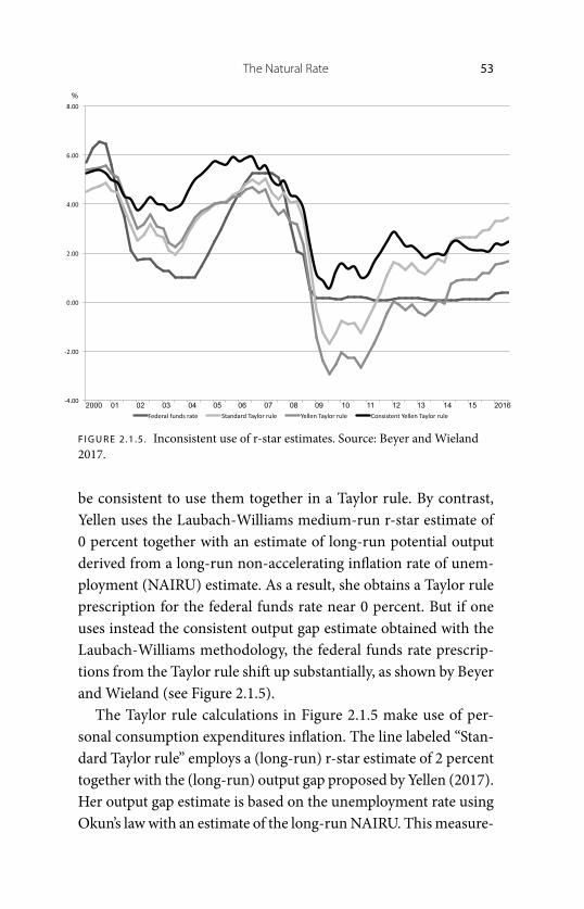
be consistent to use them together in a Taylor rule. By contrast, Yellen uses the Laubach- Williams medium- run r- star estimate of 0 percent together with an estimate of long- run potential output derived from a long- run non- accelerating infl ation rate of unem-ployment (NAIRU) estimate. As a result, she obtains a Taylor rule prescription for the federal funds rate near 0 percent. But if one uses instead the consistent output gap estimate obtained with the Laubach- Williams methodology, the federal funds rate prescrip-tions from the Taylor rule shift up substantially, as shown by Beyer and Wieland (see Figure 2.1.5).

The Taylor rule calculations in Figure 2.1.5 make use of per-sonal consumption expenditures infl ation. The line labeled “Stan-dard Taylor rule” employs a (long- run) r- star estimate of 2 percent together with the (long- run) output gap proposed by Yellen (2017). Her output gap estimate is based on the unemployment rate using Okun’s law with an estimate of the long- run NAIRU. This measure-

2000 01 02 03 04 05 06 07 08 09 10 11 12 13 14 15 2016

%

F I G U R E 2 .1 .5 . Inconsistent use of r- star estimates. Source: Beyer and Wieland 2017.

54 Wieland

ment of output gap declines following the start of the global fi nan-cial crisis, reaching a trough of −8 percent in 2010. The gap has closed in 2016. The line labeled “Yellen- Taylor rule” instead uses estimates of the medium- run r- star obtained with the Laubach- Williams method together with the long- run output gap from Yellen (2017). Finally, the darkest line uses the jointly estimated r- star and natural output level obtained with the Laubach- Williams method. The latter is quite diff erent from the Yellen estimate. Because of low estimated trend growth, the output gap closes much earlier and registers near +2 percent in 2016 and 2017. As a consequence, there is much less disagreement between the standard Taylor rule and the consistent Yellen- Taylor rule in 2016 and 2017 with levels for the federal funds rate near 2 percent.

A third concern is omitted variable bias—a point made by Taylor and Wieland (2016) and Cukierman (2016). For example, r- star estimates based on simple models consisting of an aggregate demand curve and a Phillips curve omit factors such as regulatory, fi scal, and monetary policy. If the output gap in equation (1) is lower than predicted, the method adjusts the estimate of r* downward. Similarly, if infl ation is higher than predicted by a simple Phillips curve that relates infl ation to the output gap, then the estimate of y* is adjusted downward. Yet there may be other reasons for low GDP, such as regulation reducing investment demand or tax policy reducing consumption. In equation (1) these factors are denoted by the variable x, but they are not included in the type of models estimated by Laubach and Williams and many others. Also, they omit a fi nancial sector and a central bank reaction function, which creates another relationship that makes nominal and real interest rates endogenous (see equation [3]). If the federal funds rate is not equal to the prediction from the reaction function, one can adjust the r*. However, the source of low interest rates may instead be a persistent deviation on the part of the central bank from past policy practice, as suggested by the evidence in Shin (2016) and Hofmann and Bogdanova (2012), among others.

The Natural Rate 55

ESTIMATES OF LONG- RUN R- STAR HAVE NOT DECLINED SIGNIFICANTLY

Given that frequently used estimates of a time- varying medium- run r- star suff er from great imprecision, instability, and omitted vari-able bias, it would be helpful for monetary policy to consider more structural modeling and focus on the longer run. Thus Wieland and Wolters (2017) employ two recent estimated models for the US economy in the vein of the infl uential modeling approach of Christiano, Eichenbaum, and Evans (2005): the model of Smets and Wouters (2007), which provides a complete estimation using Bayesian methods on US data, and the model of Del Negro and Schorfh eide (2015), which includes frictions and accelerator eff ects in the fi nancial sector and provides postfi nancial crisis estimates.

In these two models, the long- run equilibrium real interest rate—that is, the steady- state interest rate (r*)—is a function of trend GDP growth in steady state (ϒ ), consumer time preference (β), and intertemporal elasticity of substitution (σc):

r*c

(4)

Wieland and Wolters proceed to estimate these steady- state quantities using the two structural models. Here r* and ϒ are func-tions of other structural parameters. Estimates are infl uenced by empirical averages as well as priors for other structural parameters. Furthermore, these models show why average real interest rates might deviate from the long- run equilibrium rate over a sustained period of time.

Of course, the assumption of a constant steady state may be unrealistic. There may well be changes in long- term trends and structural breaks. Thus Wieland and Wolters estimate the mod-els for diff erent time periods (1966:1–2016:4, 1966:1–1979:1, 1966:1–2004:4, 1984:1–2016:4). Furthermore, they address the issue of structural breaks through rolling estimation. In this case,

56 Wieland

the model is based on historical data vintages, essentially every quarter, keeping the window of estimation fi xed at twenty years.

The original Smets- Wouters estimate of r* for the sample period 1966:1–2004:1 is 3 percent. This is a bit above the sample mean fed-eral funds rate of 2.65 percent for that period. Trend GDP growth per capita is 1.72 percent for that period. For a shorter sample, up to 1979:1, the estimate of the equilibrium rate is a bit smaller at 2.4 percent. Extending the sample to 2016:1 gives 2.2 percent. Just using data starting 1984:1 results in an estimate of 2.18 percent.

All these estimates are positive and signifi cantly diff erent from 0. Typical 95 percent confi dence intervals are +/− 1 percent or at most +/− 1.5 percent wide. They are substantially smaller than the confi -dence intervals for the medium- run time- varying r- star estimates.

The Del Negro and Schorfh eide model typically gives slightly smaller estimates. For example, r* is 1.75 percent for the 1966:1–2016:1 sample. Yet 95 percent confi dence intervals are a bit narrower for this model. The estimation of the Del Negro and Schorfh eide model incorporates additional data on corporate risk premiums.

Given these fi ndings, a natural conclusion would be to stick to the more precisely estimated long- run concept of the equilibrium real rate as a reference point for monetary policy. Policy rules such as the Taylor rule then prescribe higher or lower rates in response to developments in observable data such as infl ation, GDP, and GDP growth rather than an unobserved concept such as a time- varying medium- run natural real interest rate.

The real- time rolling- window estimates of Wieland and Wolt-ers (2017) shown in Figure 2.1.6 indicate that long- run r- star esti-mates change a bit over time once the sample period is limited to twenty years (solid black line). To generate these estimates, the respective model is re- estimated every quarter based on the newly available data vintage while restricting the sample period to twenty years. These estimates have declined below the 3 percent estimate from 2007 but remain above 2 percent in 2016. The decline in the

The Natural Rate 57

estimate of long- run r- star is mostly explained by a decline in the estimated trend GDP growth rate. The shaded area indicates the 95 percent confi dence interval. It implies that the estimates are pos-itive and substantially diff erent from the Laubach- Williams esti-mates of near 0 percent (dotted line).

Figure 2.1.6 also shows the average real federal funds rate over the respective twenty- year periods (dashed line). Since 2009, this average rate has declined substantially. In 2016, it takes on a value of about 0.45 percent. The structural model can be used to analyze sources of the diff erence between the average real interest rate and the estimated long- run equilibrium real interest rate. Thus, it can answer questions concerning what factors are driving these low real interest rates.

The diff erence between the twenty- year average of the real funds rate of 0.45 percent and the equilibrium real interest rate in the Smets- Wouters model (in 2016) can largely be attributed to unusually easy monetary policy and unusually high risk premiums. Specifi cally, 0.83 percent—that is, about one- half of the total dif-ference between the twenty- year average real rate and the long- run

F I G U R E 2 .1 .6 . Rolling- window estimates of long- run r- star with Smets- Wouters model. Source: Wieland and Wolters 2017.

58 Wieland

equilibrium rate—is attributed to monetary policy shocks. Another 0.48 percent, a bit more than a quarter of the diff erence, is attributed to risk- premium shocks. The risk- premium shocks lower the real rate of nominally safe assets such as Treasury bills relative to cor-porate debt, a point recently also made by Del Negro et al. (2017).

CONCLUSIONS

Yellen (2015, 2017) and Draghi (2016) have referred to the decline in estimates of time- varying (medium- run) equilibrium real inter-est rates obtained with simple IS–Phillips curve time- series models (Laubach and Williams 2003, 2016) as an important argument for keeping policy rates near zero interest- rate levels. Yet these esti-mates are highly imprecise and unstable. They do not indicate an empirically signifi cant decline and may suff er from omitted variable bias. Thus they are not that helpful for monetary policy practice. In addition, these equilibrium rate estimates are obtained jointly with estimates of potential GDP that have been below actual US GDP for a number of years.

By contrast, estimates of a long- run equilibrium rate obtained with more fully specifi ed structural macroeconomic models have not declined that much. They are positive and statistically quite diff erent from zero. The models attribute lower average real funds rates to unusually easy monetary policy and unusually high risk premiums.

With regard to the use of equilibrium real rate estimates in mon-etary policy, I would draw the following conclusions. Estimates of time- varying (medium- run) r- star should be treated with great cau-tion. It would seem better to stick to the more precisely estimated long- run concept of the equilibrium real rate as a reference point for monetary policy. Policy rules such as the Taylor rule then pre-scribe higher or lower rates in response to developments in observ-able data such as infl ation, GDP, and GDP growth rather than some

The Natural Rate 59

unobserved concept such as a time- varying medium- run natural real interest rate. Interestingly, however, if one uses the jointly esti-mated (medium- run) y- star (potential GDP) together with the (medium- run) r- star, one obtains federal funds rate prescriptions that are much closer to a rule that uses estimates of long- run equi-librium values for both. Additionally, it would be useful to con-sider a Taylor- style rule in fi rst diff erences, which therefore do not include an r- star, as a second reference point.

References

Barsky, Robert, Alejandro Justiniano, and Leonardo Melosi. 2014. “The Natural Rate of Interest and Its Usefulness for Monetary Policy.” American Economic Review 104 (5): 37–43.

Bernanke, Ben, Mark Gertler, and Simon Gilchrist. 1999. “The Financial Accelerator in a Quantitative Business Cycle Framework.” Handbook of Macro-economics 1: 1341–93.

Beyer, Robert, and Volker Wieland. 2017. “Instability, Imprecision and Inconsis-tent Use of Equilibrium Real Interest Rate Estimates.” CEPR Discussion Paper no. 11927, Center for Economic Policy Research, London.

Christiano, Lawrence, Martin Eichenbaum, and Charles L. Evans. 2005. “Nominal Rigidities and the Dynamic Eff ects of a Shock to Monetary Policy.” Journal of Political Economy 113 (1): 1–45.

Cukierman, A. 2016. “Refl ections on the Natural Rate of Interest, Its Measure-ment, Monetary Policy and the Zero Bound.” CEPR Discussion Paper no. 11467, Center for Economic Policy Research, London.

Curdia, Vasco, Andrea Ferrero, Ging Cee Ng, and Andrea Tambalotti. 2015. “Has U.S. Monetary Policy Tracked the Effi cient Interest Rate?” Journal of Monetary Economics 70:72–83.

Del Negro, Marco, Domenico Giannone, Marc Giannoni, and Andrea Tambalotti. 2017. “Safety, Liquidity, and the Natural Rate of Interest.” Federal Reserve Bank of New York, Staff Reports 812.

Del Negro, Marco, and Frank Schorfh eide. 2015. “Infl ation in the Great Recession and New Keynesian Models.” American Economic Journal: Macroeconomics 7 (1): 168–96.

60 Wieland

Draghi, M. 2016. “The International Dimension of Monetary Policy.” Presented to the ECB Forum on Central Banking, Sintra, June 28.

Garnier, J., and B.- R. Wilhelmsen. 2009. “The Natural Rate of Interest and the Output Gap in the Euro Area: A Joint Estimation.” Empirical Economics 36:297–319.

German Council of Economic Experts (GCEE). 2015. “Focus on Future Viability.” Annual Economic Report for 2015/16.

Hofmann, Boris, and Bilyana Bogdanova. 2012. “Taylor Rules and Monetary Pol-icy: A Global Great Deviation?” BIS Quarterly Review (September).

Holston, K., T. Laubach, and J. C. Williams. 2017. “Measuring the Natural Rate of Interest: International Trends and Determinants.” Journal of International Economics, forthcoming.

Krugman, Paul. 2015. “Check Out Our Low, Low (Natural) Rates.” New York Times, October 28.

Laubach, T., and J. C. Williams. 2003. “Measuring the Natural Rate of Interest.” Review of Economics and Statistics 85 (4): 1063–70.

Laubach, T., and J. C. Williams. 2016. “Measuring the Natural Rate of Interest Redux.” Business Economics 51:257–67.

Neiss, K., and E. Nelson. 2003. “The Real Interest Rate Gap as an Infl ation Indi-cator.” Macroeconomic Dynamics 7 (2): 239–62.

Shin, Hyun- Song. 2016. “Macroprudential Tools, Their Limits, and Their Con-nection with Monetary Policy.” In Progress and Confusion: The State of Macro-economic Policy, edited by Olivier Blanchard, Raghuram Rajan, Kenneth Rogoff , and Lawrence H. Summers. Cambridge, MA: MIT Press.

Smets, F., and Wouters, R. 2007. “Shocks and Frictions in US Business Cycles: A Bayesian DSGE Approach.” American Economic Review 97 (3): 586–606.

Summers, Lawrence. 2014. “U.S. Economic Prospects: Secular Stagnation, Hyster-esis, and the Zero Lower Bound.” Business Economics 49 (2): 65–73.

Taylor, John  B. 1993. “Discretion versus Policy Rules in Practice.” Carnegie- Rochester Conference Series on Public Policy 39:195–214.

Taylor, John B., and Volker Wieland. 2016. “Finding the Equilibrium Real Interest Rate in a Fog of Policy Deviations.” Business Economics 51 (3): 147–54.

Wieland, Volker, and Maik Wolters. 2017. “Little Decline in Model- Based Estimates of the Long- Run Equilibrium Interest Rate.” Working paper, IMFS.

Woodford, Michael. 2003. Interest and Prices: Foundations of a Theory of Monetary Policy. Princeton, NJ: Princeton University Press.

The Natural Rate 61

Yellen,  J. 2015. “Normalizing Monetary Policy: Prospects and Perspectives.” Remarks at the New Normal Monetary Policy conference, Federal Reserve Bank of San Francisco.

Yellen,  J. 2017. “The Economic Outlook and Conduct of Monetary Policy.” Remarks at Stanford Institute for Economic Policy Research, Stanford Uni-versity, January 19.