Embed Size (px)
Citation preview

Chapter Two
Digital Image Fundamentals
bull Agendandash Light and Electromagnetic Spectrumndash Image Sensing amp Acquisition ndash Image Sampling amp quantizationndash Relationship Between Pixelsndash Introduction to Mathematical Tools Used in DIP
Digital Image Fundamentals
Electromagnetic Spectrum
Wavelength = c (frequency )
Energy = h frequency
Definitions
bull Monochromatic (achromatic) light Light that is void of color- Attribute Intensity (amount) - Gray level is used to describe monochromatic intensity
bull Chromatic light To describe it three quantities are used- Radiance The total amount of energy that flows from the lightsource (measured in Watts)- Luminance The amount of energy an observer perceives froma light source (measured in lumens)- Brightness A subjective descriptor of light perception that isimpossible to measure (key factor in describing color sensation)
Image Sensing amp Acquisition
How to transform illumination energy into digital images
using sensing devices
Image Sensing amp Acquisition
bull Image Acquisition using single sensor
Image Sensing amp Acquisition
bull Image Acquisition using Sensor Strips
scanners
Image Sensing amp Acquisition
bull Image Acquisition using Sensor Array
Reflected Light
bull The colours that we perceive are determined by the nature of the light reflected from an object
bull For example if white light is shone onto a green object most wavelengths are absorbed while green light is reflected from the object
White Light Colours Absorb
ed
Green Light
Simple Image Formation Model
Simple image formationf(xy) = i(xy)r(xy)i(xy) illumination (determined by ill Source)
0 lt i(xy) lt infin i(xy) = 90000 lmm2 (clear day) 01lmm2 (evening)i(xy) = 10000 lmm2 (cloudy day)
r(xy) reflectance (determined by imaged object)
0 lt r(xy) lt 1 001 for black velvet065 for stainless steel
In real situationLmin le L=f(xy) le Lmax
Lmin = imin rmin Lmax = imax rmax L gray level
Image Sampling amp quantization
Image Sampling
Continues image f(xy) needs to be
in digital form
Digitizing the coordinate values called sampling
Sampling should be in both
coordinates and in amplitude
Image Sampling amp quantization
Digitizing the Amplitude values called image
quantization
Sampling limits established by no of
sensors but quantization limits by color levels
Image Quantization
Image Sampling amp quantization
Digital Image Representation
Each element called image element picture element or pixel
Image Sampling amp quantization
Image Sampling amp quantization
Image Sampling amp quantization
)11()11()01(
)11()11()01(
)10()10()00(
)(
NMfMfMf
Nfff
Nfff
yxf
The notation (01) is used to signify the second sample along the first row not the actual physical coordinates when the
image was sampled
The notation (01) is used to signify the second sample along the first row not the actual physical coordinates when the
image was sampled
Image Sampling amp quantization
Consider an image which has
M N size of the image
L Number of discrete gray levels in this image
L= 2k Where k is any positive integer
The total number of bits needed to store this image b
b = M N K
If M = N then b= N2 K
Image Sampling amp quantization
1 The dynamic range is the ratio of the max (determined by saturation) measurable intensity to the min (limited by noise) detectable intensity
2 Contrast is defined as the difference in intensity between the highest and the lowest intensity levels in an image
Image Sampling amp quantization
The dynamic range of an image can be described as
bull High dynamic range
Gray levels span a significant portion of the gray scale
bullLow dynamic range
Dull washed out gray look
Image Sampling amp quantization
bull Spatial resolution- of samples per unit length or area- Lines and distance Line pairs per unit distance
bull Gray level resolution- Number of bits per pixel- Usually 8 bits- Color image has 3 image planes to yield 8 x 3 = 24 bitspixel- Too few levels may cause false contour
Image Sampling amp quantization
Spatial Image Resolutions
No of gray levels (K) is constant(8-bits images)
No of samples (N) is reduced (No of sensors)
The subsampling was accomplished by deleting the appropriate number of rows and columns from the original image
Image Sampling amp quantization
Comparison between all image sizes
Image Sampling amp quantization
Image Sampling amp quantization
Gray Level Image Resolutions
No of samples (N) is constant but gray levels (K) decreases
(false contouring)
Image Sampling amp quantization
Little Intermediate and Large amount of details
What is the effect of changing N and K
Image Sampling amp quantization
Isopreference Curve
Interpolation is the process of using known data to estimate values at unknown locationsInterpolation is a basic tool used in tasks such as zooming shrinking rotating and geometric correctionshrinking and zooming (resampling)
Zooming requires two stepsCreation of a new pixel locationAssignment of a gray level to those new locations
Image Interpolation
Image Interpolation
bull Nearest neighbour interpolation (ex 500 x 500 image)
Laying an imaginary 750 x 750 grid over the original imageShrink it so that it fits exactly over the original imageSpacing in the grid will be less than one pixel Look for the closest pixel in the original image and assign its gray level to the new pixel in the gridFast but produces checkerboard effect
Image Interpolation
Bilinear interpolation (four neighbours of point)Let x y a point in the zoomed image v (x y) a gray level assigned to itv is given by
v (x y) = ax + by + cxy +dThe coefficients are determined from the four equations using the four neighbours
Bicubic interpolation (16 coefficeints)
Better job of preserving finer detailsStandard in commercial image editing programs
3
0
3
0
)(i j
jiij yxayxv
Image Interpolation
Relationship Between Pixels
1- Neighbors of a Pixel
The 4- neighbors of pixel p are
N4(p)
The 4- diagonal neighbors are
ND(p)
The 8-neighbors are
N8(p)
P
P
P
Relationship Between Pixels
Adjacency of Pixels-
Let V be the set of intensity used to define adjacency eg V=1 if we are referring to adjacency of pixels with value 1 in a binary image with 0 and 1In a gray-scale image for the adjacency of pixels with a range of intensity values of say 100 to 120 it follows that V=100101102hellip120We consider three types of adjacency
Adjacency
4- adjacencyTwo pixels p and q with values from V are 4- adjacency if q is in the set N4(p)
Adjacency
8- adjacencyTwo pixels p and q with values from V are 8- adjacency if q is in the set N8(p)
m- adjacency (mixed adjacency)Two pixels p and q with values from V are m- adjacency if
(i) q is in N4(p) or (ii) q is in ND ( p) and N4( p) cap N4 (q) is empty
A (digital) path(or curve) from pixel p at (xy) to pixel q at (st) is a sequence of distinct pixels with coordinates
(x0y0) (x1y1) hellip (xnyn)
where (x0y0) =(xy) (xnyn)=(st) and pixel (xiyi) and (xi-1yi-1) are adjacent for 1le i le n
n is the length of the path
If (x0y0) =(xnyn) the path is a closed path
The path can be defined 4-8-m-paths depending on adjacency type
Path
Connectivity
Let S be a subset of pixels in an image Two pixels p and q are said to be connected in S if there exists a path between them consisting entirely of pixels in SFor any pixel p in S the set of pixels that are connected to it in S is called a connected component of SIf it only has one connected component then set S is called a connected set
Region
Let R be a subset of pixels in an image We call R a region of the image if R is a connected set Two regions are said to be adjacent if their union forms a connected set
Ri Rj are adjacent in 8-adjacency senseThey are not adjacent in 4-adjacency sense
Suppose that an image contains K disjoint regions Rk k = 12 k none of which touches the image border
Let Ru be the union of all the K regions and let (Ru)c denote its complement
We call the points in Ru the foreground and all the points in (Ru)c the background of the imageThe inner boundary (border or contour) of a region R is the set of points that are adjacent to the points in the complement of R ie set of pixels in the region that have at least one background neighbour
Boundary
The point circle is not member of the border of the 1-valued region if 4-connectivity is usedAs a rule adjacency between points in a region and its background is defined in terms of 8-connectivity
Boundary
Boundary
The outer border corresponds to the border in the background This definition to guarantee the existence of a closed path
bull for pixel p q and z with coordinates
(xy) (st) and (uv) respectively
bull D is a distance function or metric if1048708 (a) D(pq) ge 0 D(pq) = 0 iff D=q
1048708 (b) D(pq) = D(qp)
1048708 (c) D(pz) le D(pq) + D(qz)
Distance Measures
1- The Euclidean distance between p and q is defined as
Distance Measures
2- The D4 distance (city-block distance) between p and q is defined as
Distance Measures
3- The D8 distance (chessboard distance) between p and q is defined as
Distance Measures
4- The Dm distance the shortest m-path between the points
Distance Measures
Array product
See matrix multiplication
2221
1211
aa
aa
2221
1211
bb
bb
22222121
12121111
2221
1211
2221
1211
baba
baba
bb
bb
aa
aa
Array Versus Matrix Operations
Linear versus Nonlinear Operations
Consider general operator H
H is said to be a linear operator if
Assume sum operator
)()( yxgyxfH
)()(
)()()()(
yxgayxga
yxfHayxfHayxfayxfaH
jjii
jjiijjii
)()(
)()(
)()()()(
yxgayxga
yxfayxfa
yxfayxfayxfayxfa
jjii
jjii
jjiijjii
Linear versus Nonlinear Operations
Let a1 = 1 a2 =-1
4-
7)1(374
56max)1(
32
20(1)max
2-
42
36max
74
56)1(
32
20)1(max
74
56 and
32
2021
ff
Arithmetic Operations
Carried out between corresponding pixel pairs
Same size of arrays
Let g(xy) denote a corrupted image formed by the addition of noise η(xy) to a noiseless image f(xy)
g(xy) = f(xy) + η(xy)
where the assumption is that at every pair of coordinates (xy) the noise is uncorrelated and has a zero average
)()()(
)()()(
)()()(
)()()(
yxgyxfyxv
yxgyxfyxp
yxgyxfyxd
yxgyxfyxs
Arithmetic Operations
If the noise satisfies the constrains just stated then an image g(xy) is formed by averaging K different noisy images
As K increases the variability of the pixels at each location decreases
)()(
2)(
2)(
1
1
1
)()(
)(1
)(
yxyxg
yxyxg
K
ii
K
K
yxfyxgE
yxgK
yxg
Arithmetic Operations
Arithmetic Operations
Image subtraction is used in the enhancement of the differences between images g(xy) = f(xy) ndash h(xy)
Arithmetic Operations
Application of image multiplication and division is shading correction
If we can get a modeled image as a product of perfect image f(xy) times a shading function h(xy) ie g(xy) = f(xy)h(xy)
If h(xy) is known we can get the perfect image f(xy)
Arithmetic Operations
Multiplication as masking
To solve the range problem in arithmetic operations we can do the following
Given an image f
fm = f ndash min(f) creates an image with min value 0 then
fs = K[fmmax(fm)] creates a scaled image whose range [0 K]
With 8-bit image setting K = 255
Logic Operations
Logic OperationAND p AND q (p q)
OR p OR q (p + q)
COMPLEMENT NOT q ( q )
Logic Operations
Spatial Operations
Performed directly on pixels
Three categoriesSingle-pixel operations
Neighbourhood operations
Geometric spatial transformation
Single-pixel operationsAlter the values of its individual pixels
s = T(z)
Spatial Operations
Neighbourhood operations
Neighbourhood processing generates a corresponding pixel at the same coordinates in an output image
R and c are the row and col Of the pixels whose coordinates are members of the set Sxy
xyScr
crfmn
yxg)(
)(1
)(
Spatial Operations
Geometric spatial transformationModify the spatial relationship between pixels in an image
Consists of two basic operations
Transformation of coordinates Expressed as (xy) = T(vw)
ex (xy) = T(vw) = (v2w2)
Affine transformation (most commonly used)
Scale rotate translate or sheer a set of coordinate points depending on the matrix T
1
0
0
111
3231
2221
1211
tt
tt
tt
wvTwvyx
Spatial Operations
Spatial Operations
The affine equation is used in two ways
Forward mappingScan pixels of the input image
At each location (vw) compute the spatial location (xy)
Two or more pixels in the input image may be transformed to the same location in the output image
Some output locations may not assign a pixel at all
Inverse mapping (more efficient used in commercial MATLAB)Scan the output pixel locations
At each location (xy) compute the spatial location (vw) = T-1(xy)
Interpolate among the nearest input pixels to determine the intensity of the output pixel value
Spatial Operations
Image Registration
Used to align two or more images of the same scene
Input and output images are available but the specific transformation function is not known
Input (image that we wish to transform)
Reference image is the image against which we want to register the input
One approach is using tie points (control points)
The location of the points are precisely known in input and reference images
Using the bilinear approximation is a simple model and given by
x = c1v+c2w+c3vw+c4
y = c5v+c6w+c7vw+c8
(xy) ndash reference image (vw) ndash input image tie points
Image Registration
Four pairs of the corresponding points -gt 8 equations to find the unknown coefficients
Image Transformation
A 2-D transform denoted T(uv) can be expressed in the general form
r(xyuv) forward transformation kernel
s(xyuv) inverse transformation kernel
1
0
1
0
)()()(M
x
N
y
vuyxryxfvuT
1
0
1
0
)()()(M
u
N
v
vuyxsvuTyxf
Image Transformation
Image Transformation
The forward transformation kernel is said to be separable if
kernel is said to be symmetric if r1(xy) is functionally equal to r2(xy) so that
2-D Fourier transform
)()()( 21 vyruxrvuyxr
)()()( 11 vyruxrvuyxr
1
0
1
0
)(2)()(M
x
N
y
NvyMuxjeyxfvuT
1
0
1
0
)(2)(1
)(M
u
N
v
NvyMuxjevuTMN
yxf
Probabilistic Methods
Treating intensities as random quantities is the simplest way of applying probability to image processing
Let zi i=012hellipL-1 possible intensities
Then the probability P(zk ) of intensity level zk is
So
Is the measure of the spread of the value of z about the mean so it is useful to measure an image contrast
MN
nzp k
k )(
1
0
22
1
0
1
0
)()(
)(
1)(
L
kkk
L
kkk
L
kk
zpmz
zpzmaveragemean
zp
Probabilistic Methods
Standard deviation is 143 316 492 intensity level
The variance is 2043 9978 24249
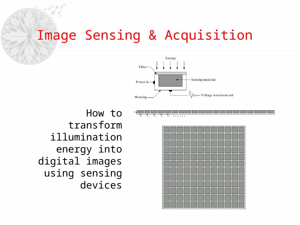
Image Sensing amp Acquisition
bull Image Acquisition using Sensor Array
Reflected Light
bull The colours that we perceive are determined by the nature of the light reflected from an object
bull For example if white light is shone onto a green object most wavelengths are absorbed while green light is reflected from the object
White Light Colours Absorb
ed
Green Light
Simple Image Formation Model
Simple image formationf(xy) = i(xy)r(xy)i(xy) illumination (determined by ill Source)
0 lt i(xy) lt infin i(xy) = 90000 lmm2 (clear day) 01lmm2 (evening)i(xy) = 10000 lmm2 (cloudy day)
r(xy) reflectance (determined by imaged object)
0 lt r(xy) lt 1 001 for black velvet065 for stainless steel
In real situationLmin le L=f(xy) le Lmax
Lmin = imin rmin Lmax = imax rmax L gray level
Image Sampling amp quantization
Image Sampling
Continues image f(xy) needs to be
in digital form
Digitizing the coordinate values called sampling
Sampling should be in both
coordinates and in amplitude
Image Sampling amp quantization
Digitizing the Amplitude values called image
quantization
Sampling limits established by no of
sensors but quantization limits by color levels
Image Quantization
Image Sampling amp quantization
Digital Image Representation
Each element called image element picture element or pixel
Image Sampling amp quantization
Image Sampling amp quantization
Image Sampling amp quantization
)11()11()01(
)11()11()01(
)10()10()00(
)(
NMfMfMf
Nfff
Nfff
yxf
The notation (01) is used to signify the second sample along the first row not the actual physical coordinates when the
image was sampled
The notation (01) is used to signify the second sample along the first row not the actual physical coordinates when the
image was sampled
Image Sampling amp quantization
Consider an image which has
M N size of the image
L Number of discrete gray levels in this image
L= 2k Where k is any positive integer
The total number of bits needed to store this image b
b = M N K
If M = N then b= N2 K
Image Sampling amp quantization
1 The dynamic range is the ratio of the max (determined by saturation) measurable intensity to the min (limited by noise) detectable intensity
2 Contrast is defined as the difference in intensity between the highest and the lowest intensity levels in an image
Image Sampling amp quantization
The dynamic range of an image can be described as
bull High dynamic range
Gray levels span a significant portion of the gray scale
bullLow dynamic range
Dull washed out gray look
Image Sampling amp quantization
bull Spatial resolution- of samples per unit length or area- Lines and distance Line pairs per unit distance
bull Gray level resolution- Number of bits per pixel- Usually 8 bits- Color image has 3 image planes to yield 8 x 3 = 24 bitspixel- Too few levels may cause false contour
Image Sampling amp quantization
Spatial Image Resolutions
No of gray levels (K) is constant(8-bits images)
No of samples (N) is reduced (No of sensors)
The subsampling was accomplished by deleting the appropriate number of rows and columns from the original image
Image Sampling amp quantization
Comparison between all image sizes
Image Sampling amp quantization
Image Sampling amp quantization
Gray Level Image Resolutions
No of samples (N) is constant but gray levels (K) decreases
(false contouring)
Image Sampling amp quantization
Little Intermediate and Large amount of details
What is the effect of changing N and K
Image Sampling amp quantization
Isopreference Curve
Interpolation is the process of using known data to estimate values at unknown locationsInterpolation is a basic tool used in tasks such as zooming shrinking rotating and geometric correctionshrinking and zooming (resampling)
Zooming requires two stepsCreation of a new pixel locationAssignment of a gray level to those new locations
Image Interpolation
Image Interpolation
bull Nearest neighbour interpolation (ex 500 x 500 image)
Laying an imaginary 750 x 750 grid over the original imageShrink it so that it fits exactly over the original imageSpacing in the grid will be less than one pixel Look for the closest pixel in the original image and assign its gray level to the new pixel in the gridFast but produces checkerboard effect
Image Interpolation
Bilinear interpolation (four neighbours of point)Let x y a point in the zoomed image v (x y) a gray level assigned to itv is given by
v (x y) = ax + by + cxy +dThe coefficients are determined from the four equations using the four neighbours
Bicubic interpolation (16 coefficeints)
Better job of preserving finer detailsStandard in commercial image editing programs
3
0
3
0
)(i j
jiij yxayxv
Image Interpolation
Relationship Between Pixels
1- Neighbors of a Pixel
The 4- neighbors of pixel p are
N4(p)
The 4- diagonal neighbors are
ND(p)
The 8-neighbors are
N8(p)
P
P
P
Relationship Between Pixels
Adjacency of Pixels-
Let V be the set of intensity used to define adjacency eg V=1 if we are referring to adjacency of pixels with value 1 in a binary image with 0 and 1In a gray-scale image for the adjacency of pixels with a range of intensity values of say 100 to 120 it follows that V=100101102hellip120We consider three types of adjacency
Adjacency
4- adjacencyTwo pixels p and q with values from V are 4- adjacency if q is in the set N4(p)
Adjacency
8- adjacencyTwo pixels p and q with values from V are 8- adjacency if q is in the set N8(p)
m- adjacency (mixed adjacency)Two pixels p and q with values from V are m- adjacency if
(i) q is in N4(p) or (ii) q is in ND ( p) and N4( p) cap N4 (q) is empty
A (digital) path(or curve) from pixel p at (xy) to pixel q at (st) is a sequence of distinct pixels with coordinates
(x0y0) (x1y1) hellip (xnyn)
where (x0y0) =(xy) (xnyn)=(st) and pixel (xiyi) and (xi-1yi-1) are adjacent for 1le i le n
n is the length of the path
If (x0y0) =(xnyn) the path is a closed path
The path can be defined 4-8-m-paths depending on adjacency type
Path
Connectivity
Let S be a subset of pixels in an image Two pixels p and q are said to be connected in S if there exists a path between them consisting entirely of pixels in SFor any pixel p in S the set of pixels that are connected to it in S is called a connected component of SIf it only has one connected component then set S is called a connected set
Region
Let R be a subset of pixels in an image We call R a region of the image if R is a connected set Two regions are said to be adjacent if their union forms a connected set
Ri Rj are adjacent in 8-adjacency senseThey are not adjacent in 4-adjacency sense
Suppose that an image contains K disjoint regions Rk k = 12 k none of which touches the image border
Let Ru be the union of all the K regions and let (Ru)c denote its complement
We call the points in Ru the foreground and all the points in (Ru)c the background of the imageThe inner boundary (border or contour) of a region R is the set of points that are adjacent to the points in the complement of R ie set of pixels in the region that have at least one background neighbour
Boundary
The point circle is not member of the border of the 1-valued region if 4-connectivity is usedAs a rule adjacency between points in a region and its background is defined in terms of 8-connectivity
Boundary
Boundary
The outer border corresponds to the border in the background This definition to guarantee the existence of a closed path
bull for pixel p q and z with coordinates
(xy) (st) and (uv) respectively
bull D is a distance function or metric if1048708 (a) D(pq) ge 0 D(pq) = 0 iff D=q
1048708 (b) D(pq) = D(qp)
1048708 (c) D(pz) le D(pq) + D(qz)
Distance Measures
1- The Euclidean distance between p and q is defined as
Distance Measures
2- The D4 distance (city-block distance) between p and q is defined as
Distance Measures
3- The D8 distance (chessboard distance) between p and q is defined as
Distance Measures
4- The Dm distance the shortest m-path between the points
Distance Measures
Array product
See matrix multiplication
2221
1211
aa
aa
2221
1211
bb
bb
22222121
12121111
2221
1211
2221
1211
baba
baba
bb
bb
aa
aa
Array Versus Matrix Operations
Linear versus Nonlinear Operations
Consider general operator H
H is said to be a linear operator if
Assume sum operator
)()( yxgyxfH
)()(
)()()()(
yxgayxga
yxfHayxfHayxfayxfaH
jjii
jjiijjii
)()(
)()(
)()()()(
yxgayxga
yxfayxfa
yxfayxfayxfayxfa
jjii
jjii
jjiijjii
Linear versus Nonlinear Operations
Let a1 = 1 a2 =-1
4-
7)1(374
56max)1(
32
20(1)max
2-
42
36max
74
56)1(
32
20)1(max
74
56 and
32
2021
ff
Arithmetic Operations
Carried out between corresponding pixel pairs
Same size of arrays
Let g(xy) denote a corrupted image formed by the addition of noise η(xy) to a noiseless image f(xy)
g(xy) = f(xy) + η(xy)
where the assumption is that at every pair of coordinates (xy) the noise is uncorrelated and has a zero average
)()()(
)()()(
)()()(
)()()(
yxgyxfyxv
yxgyxfyxp
yxgyxfyxd
yxgyxfyxs
Arithmetic Operations
If the noise satisfies the constrains just stated then an image g(xy) is formed by averaging K different noisy images
As K increases the variability of the pixels at each location decreases
)()(
2)(
2)(
1
1
1
)()(
)(1
)(
yxyxg
yxyxg
K
ii
K
K
yxfyxgE
yxgK
yxg
Arithmetic Operations
Arithmetic Operations
Image subtraction is used in the enhancement of the differences between images g(xy) = f(xy) ndash h(xy)
Arithmetic Operations
Application of image multiplication and division is shading correction
If we can get a modeled image as a product of perfect image f(xy) times a shading function h(xy) ie g(xy) = f(xy)h(xy)
If h(xy) is known we can get the perfect image f(xy)
Arithmetic Operations
Multiplication as masking
To solve the range problem in arithmetic operations we can do the following
Given an image f
fm = f ndash min(f) creates an image with min value 0 then
fs = K[fmmax(fm)] creates a scaled image whose range [0 K]
With 8-bit image setting K = 255
Logic Operations
Logic OperationAND p AND q (p q)
OR p OR q (p + q)
COMPLEMENT NOT q ( q )
Logic Operations
Spatial Operations
Performed directly on pixels
Three categoriesSingle-pixel operations
Neighbourhood operations
Geometric spatial transformation
Single-pixel operationsAlter the values of its individual pixels
s = T(z)
Spatial Operations
Neighbourhood operations
Neighbourhood processing generates a corresponding pixel at the same coordinates in an output image
R and c are the row and col Of the pixels whose coordinates are members of the set Sxy
xyScr
crfmn
yxg)(
)(1
)(
Spatial Operations
Geometric spatial transformationModify the spatial relationship between pixels in an image
Consists of two basic operations
Transformation of coordinates Expressed as (xy) = T(vw)
ex (xy) = T(vw) = (v2w2)
Affine transformation (most commonly used)
Scale rotate translate or sheer a set of coordinate points depending on the matrix T
1
0
0
111
3231
2221
1211
tt
tt
tt
wvTwvyx
Spatial Operations
Spatial Operations
The affine equation is used in two ways
Forward mappingScan pixels of the input image
At each location (vw) compute the spatial location (xy)
Two or more pixels in the input image may be transformed to the same location in the output image
Some output locations may not assign a pixel at all
Inverse mapping (more efficient used in commercial MATLAB)Scan the output pixel locations
At each location (xy) compute the spatial location (vw) = T-1(xy)
Interpolate among the nearest input pixels to determine the intensity of the output pixel value
Spatial Operations
Image Registration
Used to align two or more images of the same scene
Input and output images are available but the specific transformation function is not known
Input (image that we wish to transform)
Reference image is the image against which we want to register the input
One approach is using tie points (control points)
The location of the points are precisely known in input and reference images
Using the bilinear approximation is a simple model and given by
x = c1v+c2w+c3vw+c4
y = c5v+c6w+c7vw+c8
(xy) ndash reference image (vw) ndash input image tie points
Image Registration
Four pairs of the corresponding points -gt 8 equations to find the unknown coefficients
Image Transformation
A 2-D transform denoted T(uv) can be expressed in the general form
r(xyuv) forward transformation kernel
s(xyuv) inverse transformation kernel
1
0
1
0
)()()(M
x
N
y
vuyxryxfvuT
1
0
1
0
)()()(M
u
N
v
vuyxsvuTyxf
Image Transformation
Image Transformation
The forward transformation kernel is said to be separable if
kernel is said to be symmetric if r1(xy) is functionally equal to r2(xy) so that
2-D Fourier transform
)()()( 21 vyruxrvuyxr
)()()( 11 vyruxrvuyxr
1
0
1
0
)(2)()(M
x
N
y
NvyMuxjeyxfvuT
1
0
1
0
)(2)(1
)(M
u
N
v
NvyMuxjevuTMN
yxf
Probabilistic Methods
Treating intensities as random quantities is the simplest way of applying probability to image processing
Let zi i=012hellipL-1 possible intensities
Then the probability P(zk ) of intensity level zk is
So
Is the measure of the spread of the value of z about the mean so it is useful to measure an image contrast
MN
nzp k
k )(
1
0
22
1
0
1
0
)()(
)(
1)(
L
kkk
L
kkk
L
kk
zpmz
zpzmaveragemean
zp
Probabilistic Methods
Standard deviation is 143 316 492 intensity level
The variance is 2043 9978 24249
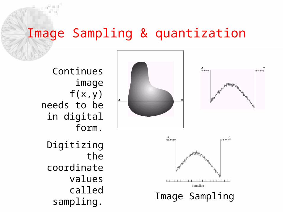
Image Sampling amp quantization
Digital Image Representation
Each element called image element picture element or pixel
Image Sampling amp quantization
Image Sampling amp quantization
Image Sampling amp quantization
)11()11()01(
)11()11()01(
)10()10()00(
)(
NMfMfMf
Nfff
Nfff
yxf
The notation (01) is used to signify the second sample along the first row not the actual physical coordinates when the
image was sampled
The notation (01) is used to signify the second sample along the first row not the actual physical coordinates when the
image was sampled
Image Sampling amp quantization
Consider an image which has
M N size of the image
L Number of discrete gray levels in this image
L= 2k Where k is any positive integer
The total number of bits needed to store this image b
b = M N K
If M = N then b= N2 K
Image Sampling amp quantization
1 The dynamic range is the ratio of the max (determined by saturation) measurable intensity to the min (limited by noise) detectable intensity
2 Contrast is defined as the difference in intensity between the highest and the lowest intensity levels in an image
Image Sampling amp quantization
The dynamic range of an image can be described as
bull High dynamic range
Gray levels span a significant portion of the gray scale
bullLow dynamic range
Dull washed out gray look
Image Sampling amp quantization
bull Spatial resolution- of samples per unit length or area- Lines and distance Line pairs per unit distance
bull Gray level resolution- Number of bits per pixel- Usually 8 bits- Color image has 3 image planes to yield 8 x 3 = 24 bitspixel- Too few levels may cause false contour
Image Sampling amp quantization
Spatial Image Resolutions
No of gray levels (K) is constant(8-bits images)
No of samples (N) is reduced (No of sensors)
The subsampling was accomplished by deleting the appropriate number of rows and columns from the original image
Image Sampling amp quantization
Comparison between all image sizes
Image Sampling amp quantization
Image Sampling amp quantization
Gray Level Image Resolutions
No of samples (N) is constant but gray levels (K) decreases
(false contouring)
Image Sampling amp quantization
Little Intermediate and Large amount of details
What is the effect of changing N and K
Image Sampling amp quantization
Isopreference Curve
Interpolation is the process of using known data to estimate values at unknown locationsInterpolation is a basic tool used in tasks such as zooming shrinking rotating and geometric correctionshrinking and zooming (resampling)
Zooming requires two stepsCreation of a new pixel locationAssignment of a gray level to those new locations
Image Interpolation
Image Interpolation
bull Nearest neighbour interpolation (ex 500 x 500 image)
Laying an imaginary 750 x 750 grid over the original imageShrink it so that it fits exactly over the original imageSpacing in the grid will be less than one pixel Look for the closest pixel in the original image and assign its gray level to the new pixel in the gridFast but produces checkerboard effect
Image Interpolation
Bilinear interpolation (four neighbours of point)Let x y a point in the zoomed image v (x y) a gray level assigned to itv is given by
v (x y) = ax + by + cxy +dThe coefficients are determined from the four equations using the four neighbours
Bicubic interpolation (16 coefficeints)
Better job of preserving finer detailsStandard in commercial image editing programs
3
0
3
0
)(i j
jiij yxayxv
Image Interpolation
Relationship Between Pixels
1- Neighbors of a Pixel
The 4- neighbors of pixel p are
N4(p)
The 4- diagonal neighbors are
ND(p)
The 8-neighbors are
N8(p)
P
P
P
Relationship Between Pixels
Adjacency of Pixels-
Let V be the set of intensity used to define adjacency eg V=1 if we are referring to adjacency of pixels with value 1 in a binary image with 0 and 1In a gray-scale image for the adjacency of pixels with a range of intensity values of say 100 to 120 it follows that V=100101102hellip120We consider three types of adjacency
Adjacency
4- adjacencyTwo pixels p and q with values from V are 4- adjacency if q is in the set N4(p)
Adjacency
8- adjacencyTwo pixels p and q with values from V are 8- adjacency if q is in the set N8(p)
m- adjacency (mixed adjacency)Two pixels p and q with values from V are m- adjacency if
(i) q is in N4(p) or (ii) q is in ND ( p) and N4( p) cap N4 (q) is empty
A (digital) path(or curve) from pixel p at (xy) to pixel q at (st) is a sequence of distinct pixels with coordinates
(x0y0) (x1y1) hellip (xnyn)
where (x0y0) =(xy) (xnyn)=(st) and pixel (xiyi) and (xi-1yi-1) are adjacent for 1le i le n
n is the length of the path
If (x0y0) =(xnyn) the path is a closed path
The path can be defined 4-8-m-paths depending on adjacency type
Path
Connectivity
Let S be a subset of pixels in an image Two pixels p and q are said to be connected in S if there exists a path between them consisting entirely of pixels in SFor any pixel p in S the set of pixels that are connected to it in S is called a connected component of SIf it only has one connected component then set S is called a connected set
Region
Let R be a subset of pixels in an image We call R a region of the image if R is a connected set Two regions are said to be adjacent if their union forms a connected set
Ri Rj are adjacent in 8-adjacency senseThey are not adjacent in 4-adjacency sense
Suppose that an image contains K disjoint regions Rk k = 12 k none of which touches the image border
Let Ru be the union of all the K regions and let (Ru)c denote its complement
We call the points in Ru the foreground and all the points in (Ru)c the background of the imageThe inner boundary (border or contour) of a region R is the set of points that are adjacent to the points in the complement of R ie set of pixels in the region that have at least one background neighbour
Boundary
The point circle is not member of the border of the 1-valued region if 4-connectivity is usedAs a rule adjacency between points in a region and its background is defined in terms of 8-connectivity
Boundary
Boundary
The outer border corresponds to the border in the background This definition to guarantee the existence of a closed path
bull for pixel p q and z with coordinates
(xy) (st) and (uv) respectively
bull D is a distance function or metric if1048708 (a) D(pq) ge 0 D(pq) = 0 iff D=q
1048708 (b) D(pq) = D(qp)
1048708 (c) D(pz) le D(pq) + D(qz)
Distance Measures
1- The Euclidean distance between p and q is defined as
Distance Measures
2- The D4 distance (city-block distance) between p and q is defined as
Distance Measures
3- The D8 distance (chessboard distance) between p and q is defined as
Distance Measures
4- The Dm distance the shortest m-path between the points
Distance Measures
Array product
See matrix multiplication
2221
1211
aa
aa
2221
1211
bb
bb
22222121
12121111
2221
1211
2221
1211
baba
baba
bb
bb
aa
aa
Array Versus Matrix Operations
Linear versus Nonlinear Operations
Consider general operator H
H is said to be a linear operator if
Assume sum operator
)()( yxgyxfH
)()(
)()()()(
yxgayxga
yxfHayxfHayxfayxfaH
jjii
jjiijjii
)()(
)()(
)()()()(
yxgayxga
yxfayxfa
yxfayxfayxfayxfa
jjii
jjii
jjiijjii
Linear versus Nonlinear Operations
Let a1 = 1 a2 =-1
4-
7)1(374
56max)1(
32
20(1)max
2-
42
36max
74
56)1(
32
20)1(max
74
56 and
32
2021
ff
Arithmetic Operations
Carried out between corresponding pixel pairs
Same size of arrays
Let g(xy) denote a corrupted image formed by the addition of noise η(xy) to a noiseless image f(xy)
g(xy) = f(xy) + η(xy)
where the assumption is that at every pair of coordinates (xy) the noise is uncorrelated and has a zero average
)()()(
)()()(
)()()(
)()()(
yxgyxfyxv
yxgyxfyxp
yxgyxfyxd
yxgyxfyxs
Arithmetic Operations
If the noise satisfies the constrains just stated then an image g(xy) is formed by averaging K different noisy images
As K increases the variability of the pixels at each location decreases
)()(
2)(
2)(
1
1
1
)()(
)(1
)(
yxyxg
yxyxg
K
ii
K
K
yxfyxgE
yxgK
yxg
Arithmetic Operations
Arithmetic Operations
Image subtraction is used in the enhancement of the differences between images g(xy) = f(xy) ndash h(xy)
Arithmetic Operations
Application of image multiplication and division is shading correction
If we can get a modeled image as a product of perfect image f(xy) times a shading function h(xy) ie g(xy) = f(xy)h(xy)
If h(xy) is known we can get the perfect image f(xy)
Arithmetic Operations
Multiplication as masking
To solve the range problem in arithmetic operations we can do the following
Given an image f
fm = f ndash min(f) creates an image with min value 0 then
fs = K[fmmax(fm)] creates a scaled image whose range [0 K]
With 8-bit image setting K = 255
Logic Operations
Logic OperationAND p AND q (p q)
OR p OR q (p + q)
COMPLEMENT NOT q ( q )
Logic Operations
Spatial Operations
Performed directly on pixels
Three categoriesSingle-pixel operations
Neighbourhood operations
Geometric spatial transformation
Single-pixel operationsAlter the values of its individual pixels
s = T(z)
Spatial Operations
Neighbourhood operations
Neighbourhood processing generates a corresponding pixel at the same coordinates in an output image
R and c are the row and col Of the pixels whose coordinates are members of the set Sxy
xyScr
crfmn
yxg)(
)(1
)(
Spatial Operations
Geometric spatial transformationModify the spatial relationship between pixels in an image
Consists of two basic operations
Transformation of coordinates Expressed as (xy) = T(vw)
ex (xy) = T(vw) = (v2w2)
Affine transformation (most commonly used)
Scale rotate translate or sheer a set of coordinate points depending on the matrix T
1
0
0
111
3231
2221
1211
tt
tt
tt
wvTwvyx
Spatial Operations
Spatial Operations
The affine equation is used in two ways
Forward mappingScan pixels of the input image
At each location (vw) compute the spatial location (xy)
Two or more pixels in the input image may be transformed to the same location in the output image
Some output locations may not assign a pixel at all
Inverse mapping (more efficient used in commercial MATLAB)Scan the output pixel locations
At each location (xy) compute the spatial location (vw) = T-1(xy)
Interpolate among the nearest input pixels to determine the intensity of the output pixel value
Spatial Operations
Image Registration
Used to align two or more images of the same scene
Input and output images are available but the specific transformation function is not known
Input (image that we wish to transform)
Reference image is the image against which we want to register the input
One approach is using tie points (control points)
The location of the points are precisely known in input and reference images
Using the bilinear approximation is a simple model and given by
x = c1v+c2w+c3vw+c4
y = c5v+c6w+c7vw+c8
(xy) ndash reference image (vw) ndash input image tie points
Image Registration
Four pairs of the corresponding points -gt 8 equations to find the unknown coefficients
Image Transformation
A 2-D transform denoted T(uv) can be expressed in the general form
r(xyuv) forward transformation kernel
s(xyuv) inverse transformation kernel
1
0
1
0
)()()(M
x
N
y
vuyxryxfvuT
1
0
1
0
)()()(M
u
N
v
vuyxsvuTyxf
Image Transformation
Image Transformation
The forward transformation kernel is said to be separable if
kernel is said to be symmetric if r1(xy) is functionally equal to r2(xy) so that
2-D Fourier transform
)()()( 21 vyruxrvuyxr
)()()( 11 vyruxrvuyxr
1
0
1
0
)(2)()(M
x
N
y
NvyMuxjeyxfvuT
1
0
1
0
)(2)(1
)(M
u
N
v
NvyMuxjevuTMN
yxf
Probabilistic Methods
Treating intensities as random quantities is the simplest way of applying probability to image processing
Let zi i=012hellipL-1 possible intensities
Then the probability P(zk ) of intensity level zk is
So
Is the measure of the spread of the value of z about the mean so it is useful to measure an image contrast
MN
nzp k
k )(
1
0
22
1
0
1
0
)()(
)(
1)(
L
kkk
L
kkk
L
kk
zpmz
zpzmaveragemean
zp
Probabilistic Methods
Standard deviation is 143 316 492 intensity level
The variance is 2043 9978 24249
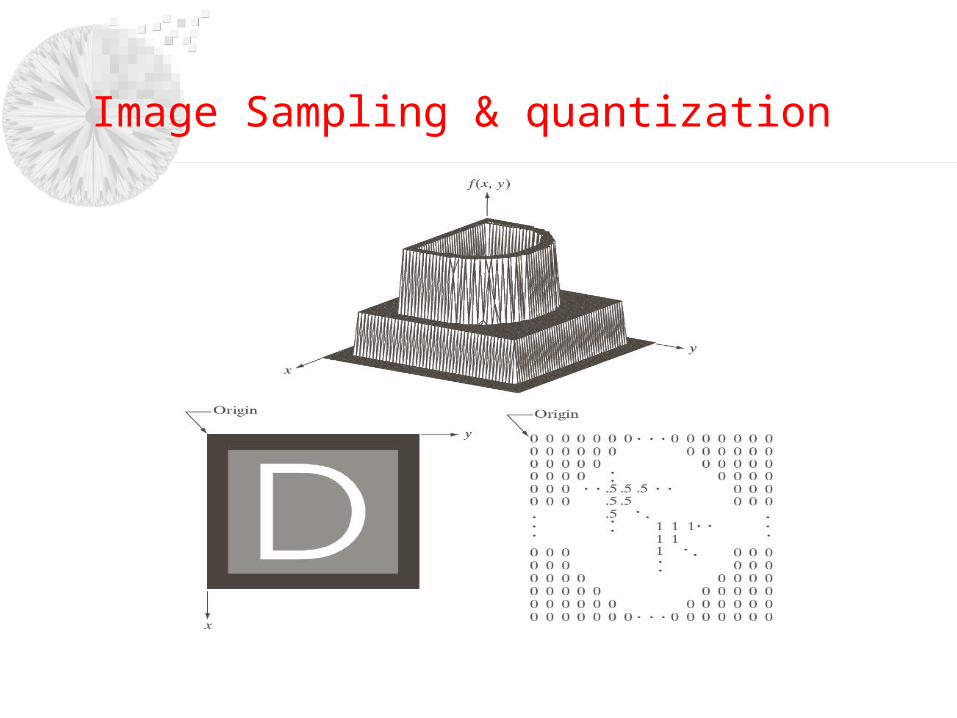
Image Sampling amp quantization
Image Sampling amp quantization
Image Sampling amp quantization
)11()11()01(
)11()11()01(
)10()10()00(
)(
NMfMfMf
Nfff
Nfff
yxf
The notation (01) is used to signify the second sample along the first row not the actual physical coordinates when the
image was sampled
The notation (01) is used to signify the second sample along the first row not the actual physical coordinates when the
image was sampled
Image Sampling amp quantization
Consider an image which has
M N size of the image
L Number of discrete gray levels in this image
L= 2k Where k is any positive integer
The total number of bits needed to store this image b
b = M N K
If M = N then b= N2 K
Image Sampling amp quantization
1 The dynamic range is the ratio of the max (determined by saturation) measurable intensity to the min (limited by noise) detectable intensity
2 Contrast is defined as the difference in intensity between the highest and the lowest intensity levels in an image
Image Sampling amp quantization
The dynamic range of an image can be described as
bull High dynamic range
Gray levels span a significant portion of the gray scale
bullLow dynamic range
Dull washed out gray look
Image Sampling amp quantization
bull Spatial resolution- of samples per unit length or area- Lines and distance Line pairs per unit distance
bull Gray level resolution- Number of bits per pixel- Usually 8 bits- Color image has 3 image planes to yield 8 x 3 = 24 bitspixel- Too few levels may cause false contour
Image Sampling amp quantization
Spatial Image Resolutions
No of gray levels (K) is constant(8-bits images)
No of samples (N) is reduced (No of sensors)
The subsampling was accomplished by deleting the appropriate number of rows and columns from the original image
Image Sampling amp quantization
Comparison between all image sizes
Image Sampling amp quantization
Image Sampling amp quantization
Gray Level Image Resolutions
No of samples (N) is constant but gray levels (K) decreases
(false contouring)
Image Sampling amp quantization
Little Intermediate and Large amount of details
What is the effect of changing N and K
Image Sampling amp quantization
Isopreference Curve
Interpolation is the process of using known data to estimate values at unknown locationsInterpolation is a basic tool used in tasks such as zooming shrinking rotating and geometric correctionshrinking and zooming (resampling)
Zooming requires two stepsCreation of a new pixel locationAssignment of a gray level to those new locations
Image Interpolation
Image Interpolation
bull Nearest neighbour interpolation (ex 500 x 500 image)
Laying an imaginary 750 x 750 grid over the original imageShrink it so that it fits exactly over the original imageSpacing in the grid will be less than one pixel Look for the closest pixel in the original image and assign its gray level to the new pixel in the gridFast but produces checkerboard effect
Image Interpolation
Bilinear interpolation (four neighbours of point)Let x y a point in the zoomed image v (x y) a gray level assigned to itv is given by
v (x y) = ax + by + cxy +dThe coefficients are determined from the four equations using the four neighbours
Bicubic interpolation (16 coefficeints)
Better job of preserving finer detailsStandard in commercial image editing programs
3
0
3
0
)(i j
jiij yxayxv
Image Interpolation
Relationship Between Pixels
1- Neighbors of a Pixel
The 4- neighbors of pixel p are
N4(p)
The 4- diagonal neighbors are
ND(p)
The 8-neighbors are
N8(p)
P
P
P
Relationship Between Pixels
Adjacency of Pixels-
Let V be the set of intensity used to define adjacency eg V=1 if we are referring to adjacency of pixels with value 1 in a binary image with 0 and 1In a gray-scale image for the adjacency of pixels with a range of intensity values of say 100 to 120 it follows that V=100101102hellip120We consider three types of adjacency
Adjacency
4- adjacencyTwo pixels p and q with values from V are 4- adjacency if q is in the set N4(p)
Adjacency
8- adjacencyTwo pixels p and q with values from V are 8- adjacency if q is in the set N8(p)
m- adjacency (mixed adjacency)Two pixels p and q with values from V are m- adjacency if
(i) q is in N4(p) or (ii) q is in ND ( p) and N4( p) cap N4 (q) is empty
A (digital) path(or curve) from pixel p at (xy) to pixel q at (st) is a sequence of distinct pixels with coordinates
(x0y0) (x1y1) hellip (xnyn)
where (x0y0) =(xy) (xnyn)=(st) and pixel (xiyi) and (xi-1yi-1) are adjacent for 1le i le n
n is the length of the path
If (x0y0) =(xnyn) the path is a closed path
The path can be defined 4-8-m-paths depending on adjacency type
Path
Connectivity
Let S be a subset of pixels in an image Two pixels p and q are said to be connected in S if there exists a path between them consisting entirely of pixels in SFor any pixel p in S the set of pixels that are connected to it in S is called a connected component of SIf it only has one connected component then set S is called a connected set
Region
Let R be a subset of pixels in an image We call R a region of the image if R is a connected set Two regions are said to be adjacent if their union forms a connected set
Ri Rj are adjacent in 8-adjacency senseThey are not adjacent in 4-adjacency sense
Suppose that an image contains K disjoint regions Rk k = 12 k none of which touches the image border
Let Ru be the union of all the K regions and let (Ru)c denote its complement
We call the points in Ru the foreground and all the points in (Ru)c the background of the imageThe inner boundary (border or contour) of a region R is the set of points that are adjacent to the points in the complement of R ie set of pixels in the region that have at least one background neighbour
Boundary
The point circle is not member of the border of the 1-valued region if 4-connectivity is usedAs a rule adjacency between points in a region and its background is defined in terms of 8-connectivity
Boundary
Boundary
The outer border corresponds to the border in the background This definition to guarantee the existence of a closed path
bull for pixel p q and z with coordinates
(xy) (st) and (uv) respectively
bull D is a distance function or metric if1048708 (a) D(pq) ge 0 D(pq) = 0 iff D=q
1048708 (b) D(pq) = D(qp)
1048708 (c) D(pz) le D(pq) + D(qz)
Distance Measures
1- The Euclidean distance between p and q is defined as
Distance Measures
2- The D4 distance (city-block distance) between p and q is defined as
Distance Measures
3- The D8 distance (chessboard distance) between p and q is defined as
Distance Measures
4- The Dm distance the shortest m-path between the points
Distance Measures
Array product
See matrix multiplication
2221
1211
aa
aa
2221
1211
bb
bb
22222121
12121111
2221
1211
2221
1211
baba
baba
bb
bb
aa
aa
Array Versus Matrix Operations
Linear versus Nonlinear Operations
Consider general operator H
H is said to be a linear operator if
Assume sum operator
)()( yxgyxfH
)()(
)()()()(
yxgayxga
yxfHayxfHayxfayxfaH
jjii
jjiijjii
)()(
)()(
)()()()(
yxgayxga
yxfayxfa
yxfayxfayxfayxfa
jjii
jjii
jjiijjii
Linear versus Nonlinear Operations
Let a1 = 1 a2 =-1
4-
7)1(374
56max)1(
32
20(1)max
2-
42
36max
74
56)1(
32
20)1(max
74
56 and
32
2021
ff
Arithmetic Operations
Carried out between corresponding pixel pairs
Same size of arrays
Let g(xy) denote a corrupted image formed by the addition of noise η(xy) to a noiseless image f(xy)
g(xy) = f(xy) + η(xy)
where the assumption is that at every pair of coordinates (xy) the noise is uncorrelated and has a zero average
)()()(
)()()(
)()()(
)()()(
yxgyxfyxv
yxgyxfyxp
yxgyxfyxd
yxgyxfyxs
Arithmetic Operations
If the noise satisfies the constrains just stated then an image g(xy) is formed by averaging K different noisy images
As K increases the variability of the pixels at each location decreases
)()(
2)(
2)(
1
1
1
)()(
)(1
)(
yxyxg
yxyxg
K
ii
K
K
yxfyxgE
yxgK
yxg
Arithmetic Operations
Arithmetic Operations
Image subtraction is used in the enhancement of the differences between images g(xy) = f(xy) ndash h(xy)
Arithmetic Operations
Application of image multiplication and division is shading correction
If we can get a modeled image as a product of perfect image f(xy) times a shading function h(xy) ie g(xy) = f(xy)h(xy)
If h(xy) is known we can get the perfect image f(xy)
Arithmetic Operations
Multiplication as masking
To solve the range problem in arithmetic operations we can do the following
Given an image f
fm = f ndash min(f) creates an image with min value 0 then
fs = K[fmmax(fm)] creates a scaled image whose range [0 K]
With 8-bit image setting K = 255
Logic Operations
Logic OperationAND p AND q (p q)
OR p OR q (p + q)
COMPLEMENT NOT q ( q )
Logic Operations
Spatial Operations
Performed directly on pixels
Three categoriesSingle-pixel operations
Neighbourhood operations
Geometric spatial transformation
Single-pixel operationsAlter the values of its individual pixels
s = T(z)
Spatial Operations
Neighbourhood operations
Neighbourhood processing generates a corresponding pixel at the same coordinates in an output image
R and c are the row and col Of the pixels whose coordinates are members of the set Sxy
xyScr
crfmn
yxg)(
)(1
)(
Spatial Operations
Geometric spatial transformationModify the spatial relationship between pixels in an image
Consists of two basic operations
Transformation of coordinates Expressed as (xy) = T(vw)
ex (xy) = T(vw) = (v2w2)
Affine transformation (most commonly used)
Scale rotate translate or sheer a set of coordinate points depending on the matrix T
1
0
0
111
3231
2221
1211
tt
tt
tt
wvTwvyx
Spatial Operations
Spatial Operations
The affine equation is used in two ways
Forward mappingScan pixels of the input image
At each location (vw) compute the spatial location (xy)
Two or more pixels in the input image may be transformed to the same location in the output image
Some output locations may not assign a pixel at all
Inverse mapping (more efficient used in commercial MATLAB)Scan the output pixel locations
At each location (xy) compute the spatial location (vw) = T-1(xy)
Interpolate among the nearest input pixels to determine the intensity of the output pixel value
Spatial Operations
Image Registration
Used to align two or more images of the same scene
Input and output images are available but the specific transformation function is not known
Input (image that we wish to transform)
Reference image is the image against which we want to register the input
One approach is using tie points (control points)
The location of the points are precisely known in input and reference images
Using the bilinear approximation is a simple model and given by
x = c1v+c2w+c3vw+c4
y = c5v+c6w+c7vw+c8
(xy) ndash reference image (vw) ndash input image tie points
Image Registration
Four pairs of the corresponding points -gt 8 equations to find the unknown coefficients
Image Transformation
A 2-D transform denoted T(uv) can be expressed in the general form
r(xyuv) forward transformation kernel
s(xyuv) inverse transformation kernel
1
0
1
0
)()()(M
x
N
y
vuyxryxfvuT
1
0
1
0
)()()(M
u
N
v
vuyxsvuTyxf
Image Transformation
Image Transformation
The forward transformation kernel is said to be separable if
kernel is said to be symmetric if r1(xy) is functionally equal to r2(xy) so that
2-D Fourier transform
)()()( 21 vyruxrvuyxr
)()()( 11 vyruxrvuyxr
1
0
1
0
)(2)()(M
x
N
y
NvyMuxjeyxfvuT
1
0
1
0
)(2)(1
)(M
u
N
v
NvyMuxjevuTMN
yxf
Probabilistic Methods
Treating intensities as random quantities is the simplest way of applying probability to image processing
Let zi i=012hellipL-1 possible intensities
Then the probability P(zk ) of intensity level zk is
So
Is the measure of the spread of the value of z about the mean so it is useful to measure an image contrast
MN
nzp k
k )(
1
0
22
1
0
1
0
)()(
)(
1)(
L
kkk
L
kkk
L
kk
zpmz
zpzmaveragemean
zp
Probabilistic Methods
Standard deviation is 143 316 492 intensity level
The variance is 2043 9978 24249
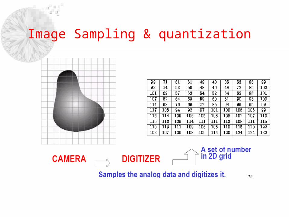
Image Sampling amp quantization
Image Sampling amp quantization
)11()11()01(
)11()11()01(
)10()10()00(
)(
NMfMfMf
Nfff
Nfff
yxf
The notation (01) is used to signify the second sample along the first row not the actual physical coordinates when the
image was sampled
The notation (01) is used to signify the second sample along the first row not the actual physical coordinates when the
image was sampled
Image Sampling amp quantization
Consider an image which has
M N size of the image
L Number of discrete gray levels in this image
L= 2k Where k is any positive integer
The total number of bits needed to store this image b
b = M N K
If M = N then b= N2 K
Image Sampling amp quantization
1 The dynamic range is the ratio of the max (determined by saturation) measurable intensity to the min (limited by noise) detectable intensity
2 Contrast is defined as the difference in intensity between the highest and the lowest intensity levels in an image
Image Sampling amp quantization
The dynamic range of an image can be described as
bull High dynamic range
Gray levels span a significant portion of the gray scale
bullLow dynamic range
Dull washed out gray look
Image Sampling amp quantization
bull Spatial resolution- of samples per unit length or area- Lines and distance Line pairs per unit distance
bull Gray level resolution- Number of bits per pixel- Usually 8 bits- Color image has 3 image planes to yield 8 x 3 = 24 bitspixel- Too few levels may cause false contour
Image Sampling amp quantization
Spatial Image Resolutions
No of gray levels (K) is constant(8-bits images)
No of samples (N) is reduced (No of sensors)
The subsampling was accomplished by deleting the appropriate number of rows and columns from the original image
Image Sampling amp quantization
Comparison between all image sizes
Image Sampling amp quantization
Image Sampling amp quantization
Gray Level Image Resolutions
No of samples (N) is constant but gray levels (K) decreases
(false contouring)
Image Sampling amp quantization
Little Intermediate and Large amount of details
What is the effect of changing N and K
Image Sampling amp quantization
Isopreference Curve
Interpolation is the process of using known data to estimate values at unknown locationsInterpolation is a basic tool used in tasks such as zooming shrinking rotating and geometric correctionshrinking and zooming (resampling)
Zooming requires two stepsCreation of a new pixel locationAssignment of a gray level to those new locations
Image Interpolation
Image Interpolation
bull Nearest neighbour interpolation (ex 500 x 500 image)
Laying an imaginary 750 x 750 grid over the original imageShrink it so that it fits exactly over the original imageSpacing in the grid will be less than one pixel Look for the closest pixel in the original image and assign its gray level to the new pixel in the gridFast but produces checkerboard effect
Image Interpolation
Bilinear interpolation (four neighbours of point)Let x y a point in the zoomed image v (x y) a gray level assigned to itv is given by
v (x y) = ax + by + cxy +dThe coefficients are determined from the four equations using the four neighbours
Bicubic interpolation (16 coefficeints)
Better job of preserving finer detailsStandard in commercial image editing programs
3
0
3
0
)(i j
jiij yxayxv
Image Interpolation
Relationship Between Pixels
1- Neighbors of a Pixel
The 4- neighbors of pixel p are
N4(p)
The 4- diagonal neighbors are
ND(p)
The 8-neighbors are
N8(p)
P
P
P
Relationship Between Pixels
Adjacency of Pixels-
Let V be the set of intensity used to define adjacency eg V=1 if we are referring to adjacency of pixels with value 1 in a binary image with 0 and 1In a gray-scale image for the adjacency of pixels with a range of intensity values of say 100 to 120 it follows that V=100101102hellip120We consider three types of adjacency
Adjacency
4- adjacencyTwo pixels p and q with values from V are 4- adjacency if q is in the set N4(p)
Adjacency
8- adjacencyTwo pixels p and q with values from V are 8- adjacency if q is in the set N8(p)
m- adjacency (mixed adjacency)Two pixels p and q with values from V are m- adjacency if
(i) q is in N4(p) or (ii) q is in ND ( p) and N4( p) cap N4 (q) is empty
A (digital) path(or curve) from pixel p at (xy) to pixel q at (st) is a sequence of distinct pixels with coordinates
(x0y0) (x1y1) hellip (xnyn)
where (x0y0) =(xy) (xnyn)=(st) and pixel (xiyi) and (xi-1yi-1) are adjacent for 1le i le n
n is the length of the path
If (x0y0) =(xnyn) the path is a closed path
The path can be defined 4-8-m-paths depending on adjacency type
Path
Connectivity
Let S be a subset of pixels in an image Two pixels p and q are said to be connected in S if there exists a path between them consisting entirely of pixels in SFor any pixel p in S the set of pixels that are connected to it in S is called a connected component of SIf it only has one connected component then set S is called a connected set
Region
Let R be a subset of pixels in an image We call R a region of the image if R is a connected set Two regions are said to be adjacent if their union forms a connected set
Ri Rj are adjacent in 8-adjacency senseThey are not adjacent in 4-adjacency sense
Suppose that an image contains K disjoint regions Rk k = 12 k none of which touches the image border
Let Ru be the union of all the K regions and let (Ru)c denote its complement
We call the points in Ru the foreground and all the points in (Ru)c the background of the imageThe inner boundary (border or contour) of a region R is the set of points that are adjacent to the points in the complement of R ie set of pixels in the region that have at least one background neighbour
Boundary
The point circle is not member of the border of the 1-valued region if 4-connectivity is usedAs a rule adjacency between points in a region and its background is defined in terms of 8-connectivity
Boundary
Boundary
The outer border corresponds to the border in the background This definition to guarantee the existence of a closed path
bull for pixel p q and z with coordinates
(xy) (st) and (uv) respectively
bull D is a distance function or metric if1048708 (a) D(pq) ge 0 D(pq) = 0 iff D=q
1048708 (b) D(pq) = D(qp)
1048708 (c) D(pz) le D(pq) + D(qz)
Distance Measures
1- The Euclidean distance between p and q is defined as
Distance Measures
2- The D4 distance (city-block distance) between p and q is defined as
Distance Measures
3- The D8 distance (chessboard distance) between p and q is defined as
Distance Measures
4- The Dm distance the shortest m-path between the points
Distance Measures
Array product
See matrix multiplication
2221
1211
aa
aa
2221
1211
bb
bb
22222121
12121111
2221
1211
2221
1211
baba
baba
bb
bb
aa
aa
Array Versus Matrix Operations
Linear versus Nonlinear Operations
Consider general operator H
H is said to be a linear operator if
Assume sum operator
)()( yxgyxfH
)()(
)()()()(
yxgayxga
yxfHayxfHayxfayxfaH
jjii
jjiijjii
)()(
)()(
)()()()(
yxgayxga
yxfayxfa
yxfayxfayxfayxfa
jjii
jjii
jjiijjii
Linear versus Nonlinear Operations
Let a1 = 1 a2 =-1
4-
7)1(374
56max)1(
32
20(1)max
2-
42
36max
74
56)1(
32
20)1(max
74
56 and
32
2021
ff
Arithmetic Operations
Carried out between corresponding pixel pairs
Same size of arrays
Let g(xy) denote a corrupted image formed by the addition of noise η(xy) to a noiseless image f(xy)
g(xy) = f(xy) + η(xy)
where the assumption is that at every pair of coordinates (xy) the noise is uncorrelated and has a zero average
)()()(
)()()(
)()()(
)()()(
yxgyxfyxv
yxgyxfyxp
yxgyxfyxd
yxgyxfyxs
Arithmetic Operations
If the noise satisfies the constrains just stated then an image g(xy) is formed by averaging K different noisy images
As K increases the variability of the pixels at each location decreases
)()(
2)(
2)(
1
1
1
)()(
)(1
)(
yxyxg
yxyxg
K
ii
K
K
yxfyxgE
yxgK
yxg
Arithmetic Operations
Arithmetic Operations
Image subtraction is used in the enhancement of the differences between images g(xy) = f(xy) ndash h(xy)
Arithmetic Operations
Application of image multiplication and division is shading correction
If we can get a modeled image as a product of perfect image f(xy) times a shading function h(xy) ie g(xy) = f(xy)h(xy)
If h(xy) is known we can get the perfect image f(xy)
Arithmetic Operations
Multiplication as masking
To solve the range problem in arithmetic operations we can do the following
Given an image f
fm = f ndash min(f) creates an image with min value 0 then
fs = K[fmmax(fm)] creates a scaled image whose range [0 K]
With 8-bit image setting K = 255
Logic Operations
Logic OperationAND p AND q (p q)
OR p OR q (p + q)
COMPLEMENT NOT q ( q )
Logic Operations
Spatial Operations
Performed directly on pixels
Three categoriesSingle-pixel operations
Neighbourhood operations
Geometric spatial transformation
Single-pixel operationsAlter the values of its individual pixels
s = T(z)
Spatial Operations
Neighbourhood operations
Neighbourhood processing generates a corresponding pixel at the same coordinates in an output image
R and c are the row and col Of the pixels whose coordinates are members of the set Sxy
xyScr
crfmn
yxg)(
)(1
)(
Spatial Operations
Geometric spatial transformationModify the spatial relationship between pixels in an image
Consists of two basic operations
Transformation of coordinates Expressed as (xy) = T(vw)
ex (xy) = T(vw) = (v2w2)
Affine transformation (most commonly used)
Scale rotate translate or sheer a set of coordinate points depending on the matrix T
1
0
0
111
3231
2221
1211
tt
tt
tt
wvTwvyx
Spatial Operations
Spatial Operations
The affine equation is used in two ways
Forward mappingScan pixels of the input image
At each location (vw) compute the spatial location (xy)
Two or more pixels in the input image may be transformed to the same location in the output image
Some output locations may not assign a pixel at all
Inverse mapping (more efficient used in commercial MATLAB)Scan the output pixel locations
At each location (xy) compute the spatial location (vw) = T-1(xy)
Interpolate among the nearest input pixels to determine the intensity of the output pixel value
Spatial Operations
Image Registration
Used to align two or more images of the same scene
Input and output images are available but the specific transformation function is not known
Input (image that we wish to transform)
Reference image is the image against which we want to register the input
One approach is using tie points (control points)
The location of the points are precisely known in input and reference images
Using the bilinear approximation is a simple model and given by
x = c1v+c2w+c3vw+c4
y = c5v+c6w+c7vw+c8
(xy) ndash reference image (vw) ndash input image tie points
Image Registration
Four pairs of the corresponding points -gt 8 equations to find the unknown coefficients
Image Transformation
A 2-D transform denoted T(uv) can be expressed in the general form
r(xyuv) forward transformation kernel
s(xyuv) inverse transformation kernel
1
0
1
0
)()()(M
x
N
y
vuyxryxfvuT
1
0
1
0
)()()(M
u
N
v
vuyxsvuTyxf
Image Transformation
Image Transformation
The forward transformation kernel is said to be separable if
kernel is said to be symmetric if r1(xy) is functionally equal to r2(xy) so that
2-D Fourier transform
)()()( 21 vyruxrvuyxr
)()()( 11 vyruxrvuyxr
1
0
1
0
)(2)()(M
x
N
y
NvyMuxjeyxfvuT
1
0
1
0
)(2)(1
)(M
u
N
v
NvyMuxjevuTMN
yxf
Probabilistic Methods
Treating intensities as random quantities is the simplest way of applying probability to image processing
Let zi i=012hellipL-1 possible intensities
Then the probability P(zk ) of intensity level zk is
So
Is the measure of the spread of the value of z about the mean so it is useful to measure an image contrast
MN
nzp k
k )(
1
0
22
1
0
1
0
)()(
)(
1)(
L
kkk
L
kkk
L
kk
zpmz
zpzmaveragemean
zp
Probabilistic Methods
Standard deviation is 143 316 492 intensity level
The variance is 2043 9978 24249
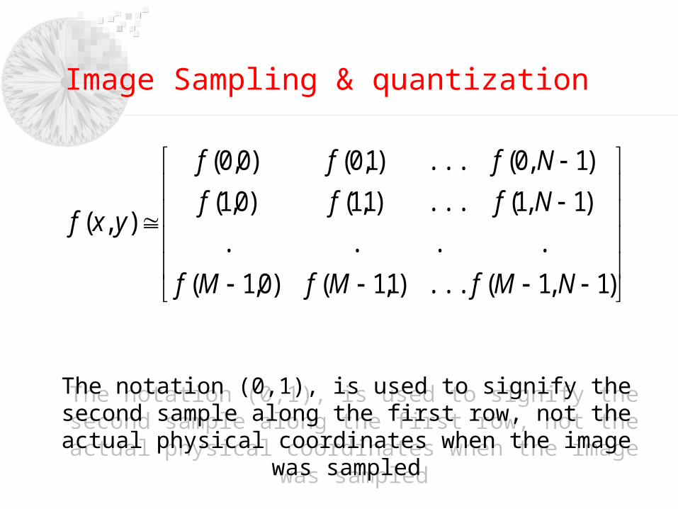
Image Sampling amp quantization
)11()11()01(
)11()11()01(
)10()10()00(
)(
NMfMfMf
Nfff
Nfff
yxf
The notation (01) is used to signify the second sample along the first row not the actual physical coordinates when the
image was sampled
The notation (01) is used to signify the second sample along the first row not the actual physical coordinates when the
image was sampled
Image Sampling amp quantization
Consider an image which has
M N size of the image
L Number of discrete gray levels in this image
L= 2k Where k is any positive integer
The total number of bits needed to store this image b
b = M N K
If M = N then b= N2 K
Image Sampling amp quantization
1 The dynamic range is the ratio of the max (determined by saturation) measurable intensity to the min (limited by noise) detectable intensity
2 Contrast is defined as the difference in intensity between the highest and the lowest intensity levels in an image
Image Sampling amp quantization
The dynamic range of an image can be described as
bull High dynamic range
Gray levels span a significant portion of the gray scale
bullLow dynamic range
Dull washed out gray look
Image Sampling amp quantization
bull Spatial resolution- of samples per unit length or area- Lines and distance Line pairs per unit distance
bull Gray level resolution- Number of bits per pixel- Usually 8 bits- Color image has 3 image planes to yield 8 x 3 = 24 bitspixel- Too few levels may cause false contour
Image Sampling amp quantization
Spatial Image Resolutions
No of gray levels (K) is constant(8-bits images)
No of samples (N) is reduced (No of sensors)
The subsampling was accomplished by deleting the appropriate number of rows and columns from the original image
Image Sampling amp quantization
Comparison between all image sizes
Image Sampling amp quantization
Image Sampling amp quantization
Gray Level Image Resolutions
No of samples (N) is constant but gray levels (K) decreases
(false contouring)
Image Sampling amp quantization
Little Intermediate and Large amount of details
What is the effect of changing N and K
Image Sampling amp quantization
Isopreference Curve
Interpolation is the process of using known data to estimate values at unknown locationsInterpolation is a basic tool used in tasks such as zooming shrinking rotating and geometric correctionshrinking and zooming (resampling)
Zooming requires two stepsCreation of a new pixel locationAssignment of a gray level to those new locations
Image Interpolation
Image Interpolation
bull Nearest neighbour interpolation (ex 500 x 500 image)
Laying an imaginary 750 x 750 grid over the original imageShrink it so that it fits exactly over the original imageSpacing in the grid will be less than one pixel Look for the closest pixel in the original image and assign its gray level to the new pixel in the gridFast but produces checkerboard effect
Image Interpolation
Bilinear interpolation (four neighbours of point)Let x y a point in the zoomed image v (x y) a gray level assigned to itv is given by
v (x y) = ax + by + cxy +dThe coefficients are determined from the four equations using the four neighbours
Bicubic interpolation (16 coefficeints)
Better job of preserving finer detailsStandard in commercial image editing programs
3
0
3
0
)(i j
jiij yxayxv
Image Interpolation
Relationship Between Pixels
1- Neighbors of a Pixel
The 4- neighbors of pixel p are
N4(p)
The 4- diagonal neighbors are
ND(p)
The 8-neighbors are
N8(p)
P
P
P
Relationship Between Pixels
Adjacency of Pixels-
Let V be the set of intensity used to define adjacency eg V=1 if we are referring to adjacency of pixels with value 1 in a binary image with 0 and 1In a gray-scale image for the adjacency of pixels with a range of intensity values of say 100 to 120 it follows that V=100101102hellip120We consider three types of adjacency
Adjacency
4- adjacencyTwo pixels p and q with values from V are 4- adjacency if q is in the set N4(p)
Adjacency
8- adjacencyTwo pixels p and q with values from V are 8- adjacency if q is in the set N8(p)
m- adjacency (mixed adjacency)Two pixels p and q with values from V are m- adjacency if
(i) q is in N4(p) or (ii) q is in ND ( p) and N4( p) cap N4 (q) is empty
A (digital) path(or curve) from pixel p at (xy) to pixel q at (st) is a sequence of distinct pixels with coordinates
(x0y0) (x1y1) hellip (xnyn)
where (x0y0) =(xy) (xnyn)=(st) and pixel (xiyi) and (xi-1yi-1) are adjacent for 1le i le n
n is the length of the path
If (x0y0) =(xnyn) the path is a closed path
The path can be defined 4-8-m-paths depending on adjacency type
Path
Connectivity
Let S be a subset of pixels in an image Two pixels p and q are said to be connected in S if there exists a path between them consisting entirely of pixels in SFor any pixel p in S the set of pixels that are connected to it in S is called a connected component of SIf it only has one connected component then set S is called a connected set
Region
Let R be a subset of pixels in an image We call R a region of the image if R is a connected set Two regions are said to be adjacent if their union forms a connected set
Ri Rj are adjacent in 8-adjacency senseThey are not adjacent in 4-adjacency sense
Suppose that an image contains K disjoint regions Rk k = 12 k none of which touches the image border
Let Ru be the union of all the K regions and let (Ru)c denote its complement
We call the points in Ru the foreground and all the points in (Ru)c the background of the imageThe inner boundary (border or contour) of a region R is the set of points that are adjacent to the points in the complement of R ie set of pixels in the region that have at least one background neighbour
Boundary
The point circle is not member of the border of the 1-valued region if 4-connectivity is usedAs a rule adjacency between points in a region and its background is defined in terms of 8-connectivity
Boundary
Boundary
The outer border corresponds to the border in the background This definition to guarantee the existence of a closed path
bull for pixel p q and z with coordinates
(xy) (st) and (uv) respectively
bull D is a distance function or metric if1048708 (a) D(pq) ge 0 D(pq) = 0 iff D=q
1048708 (b) D(pq) = D(qp)
1048708 (c) D(pz) le D(pq) + D(qz)
Distance Measures
1- The Euclidean distance between p and q is defined as
Distance Measures
2- The D4 distance (city-block distance) between p and q is defined as
Distance Measures
3- The D8 distance (chessboard distance) between p and q is defined as
Distance Measures
4- The Dm distance the shortest m-path between the points
Distance Measures
Array product
See matrix multiplication
2221
1211
aa
aa
2221
1211
bb
bb
22222121
12121111
2221
1211
2221
1211
baba
baba
bb
bb
aa
aa
Array Versus Matrix Operations
Linear versus Nonlinear Operations
Consider general operator H
H is said to be a linear operator if
Assume sum operator
)()( yxgyxfH
)()(
)()()()(
yxgayxga
yxfHayxfHayxfayxfaH
jjii
jjiijjii
)()(
)()(
)()()()(
yxgayxga
yxfayxfa
yxfayxfayxfayxfa
jjii
jjii
jjiijjii
Linear versus Nonlinear Operations
Let a1 = 1 a2 =-1
4-
7)1(374
56max)1(
32
20(1)max
2-
42
36max
74
56)1(
32
20)1(max
74
56 and
32
2021
ff
Arithmetic Operations
Carried out between corresponding pixel pairs
Same size of arrays
Let g(xy) denote a corrupted image formed by the addition of noise η(xy) to a noiseless image f(xy)
g(xy) = f(xy) + η(xy)
where the assumption is that at every pair of coordinates (xy) the noise is uncorrelated and has a zero average
)()()(
)()()(
)()()(
)()()(
yxgyxfyxv
yxgyxfyxp
yxgyxfyxd
yxgyxfyxs
Arithmetic Operations
If the noise satisfies the constrains just stated then an image g(xy) is formed by averaging K different noisy images
As K increases the variability of the pixels at each location decreases
)()(
2)(
2)(
1
1
1
)()(
)(1
)(
yxyxg
yxyxg
K
ii
K
K
yxfyxgE
yxgK
yxg
Arithmetic Operations
Arithmetic Operations
Image subtraction is used in the enhancement of the differences between images g(xy) = f(xy) ndash h(xy)
Arithmetic Operations
Application of image multiplication and division is shading correction
If we can get a modeled image as a product of perfect image f(xy) times a shading function h(xy) ie g(xy) = f(xy)h(xy)
If h(xy) is known we can get the perfect image f(xy)
Arithmetic Operations
Multiplication as masking
To solve the range problem in arithmetic operations we can do the following
Given an image f
fm = f ndash min(f) creates an image with min value 0 then
fs = K[fmmax(fm)] creates a scaled image whose range [0 K]
With 8-bit image setting K = 255
Logic Operations
Logic OperationAND p AND q (p q)
OR p OR q (p + q)
COMPLEMENT NOT q ( q )
Logic Operations
Spatial Operations
Performed directly on pixels
Three categoriesSingle-pixel operations
Neighbourhood operations
Geometric spatial transformation
Single-pixel operationsAlter the values of its individual pixels
s = T(z)
Spatial Operations
Neighbourhood operations
Neighbourhood processing generates a corresponding pixel at the same coordinates in an output image
R and c are the row and col Of the pixels whose coordinates are members of the set Sxy
xyScr
crfmn
yxg)(
)(1
)(
Spatial Operations
Geometric spatial transformationModify the spatial relationship between pixels in an image
Consists of two basic operations
Transformation of coordinates Expressed as (xy) = T(vw)
ex (xy) = T(vw) = (v2w2)
Affine transformation (most commonly used)
Scale rotate translate or sheer a set of coordinate points depending on the matrix T
1
0
0
111
3231
2221
1211
tt
tt
tt
wvTwvyx
Spatial Operations
Spatial Operations
The affine equation is used in two ways
Forward mappingScan pixels of the input image
At each location (vw) compute the spatial location (xy)
Two or more pixels in the input image may be transformed to the same location in the output image
Some output locations may not assign a pixel at all
Inverse mapping (more efficient used in commercial MATLAB)Scan the output pixel locations
At each location (xy) compute the spatial location (vw) = T-1(xy)
Interpolate among the nearest input pixels to determine the intensity of the output pixel value
Spatial Operations
Image Registration
Used to align two or more images of the same scene
Input and output images are available but the specific transformation function is not known
Input (image that we wish to transform)
Reference image is the image against which we want to register the input
One approach is using tie points (control points)
The location of the points are precisely known in input and reference images
Using the bilinear approximation is a simple model and given by
x = c1v+c2w+c3vw+c4
y = c5v+c6w+c7vw+c8
(xy) ndash reference image (vw) ndash input image tie points
Image Registration
Four pairs of the corresponding points -gt 8 equations to find the unknown coefficients
Image Transformation
A 2-D transform denoted T(uv) can be expressed in the general form
r(xyuv) forward transformation kernel
s(xyuv) inverse transformation kernel
1
0
1
0
)()()(M
x
N
y
vuyxryxfvuT
1
0
1
0
)()()(M
u
N
v
vuyxsvuTyxf
Image Transformation
Image Transformation
The forward transformation kernel is said to be separable if
kernel is said to be symmetric if r1(xy) is functionally equal to r2(xy) so that
2-D Fourier transform
)()()( 21 vyruxrvuyxr
)()()( 11 vyruxrvuyxr
1
0
1
0
)(2)()(M
x
N
y
NvyMuxjeyxfvuT
1
0
1
0
)(2)(1
)(M
u
N
v
NvyMuxjevuTMN
yxf
Probabilistic Methods
Treating intensities as random quantities is the simplest way of applying probability to image processing
Let zi i=012hellipL-1 possible intensities
Then the probability P(zk ) of intensity level zk is
So
Is the measure of the spread of the value of z about the mean so it is useful to measure an image contrast
MN
nzp k
k )(
1
0
22
1
0
1
0
)()(
)(
1)(
L
kkk
L
kkk
L
kk
zpmz
zpzmaveragemean
zp
Probabilistic Methods
Standard deviation is 143 316 492 intensity level
The variance is 2043 9978 24249

Image Sampling amp quantization
bull Spatial resolution- of samples per unit length or area- Lines and distance Line pairs per unit distance
bull Gray level resolution- Number of bits per pixel- Usually 8 bits- Color image has 3 image planes to yield 8 x 3 = 24 bitspixel- Too few levels may cause false contour
Image Sampling amp quantization
Spatial Image Resolutions
No of gray levels (K) is constant(8-bits images)
No of samples (N) is reduced (No of sensors)
The subsampling was accomplished by deleting the appropriate number of rows and columns from the original image
Image Sampling amp quantization
Comparison between all image sizes
Image Sampling amp quantization
Image Sampling amp quantization
Gray Level Image Resolutions
No of samples (N) is constant but gray levels (K) decreases
(false contouring)
Image Sampling amp quantization
Little Intermediate and Large amount of details
What is the effect of changing N and K
Image Sampling amp quantization
Isopreference Curve
Interpolation is the process of using known data to estimate values at unknown locationsInterpolation is a basic tool used in tasks such as zooming shrinking rotating and geometric correctionshrinking and zooming (resampling)
Zooming requires two stepsCreation of a new pixel locationAssignment of a gray level to those new locations
Image Interpolation
Image Interpolation
bull Nearest neighbour interpolation (ex 500 x 500 image)
Laying an imaginary 750 x 750 grid over the original imageShrink it so that it fits exactly over the original imageSpacing in the grid will be less than one pixel Look for the closest pixel in the original image and assign its gray level to the new pixel in the gridFast but produces checkerboard effect
Image Interpolation
Bilinear interpolation (four neighbours of point)Let x y a point in the zoomed image v (x y) a gray level assigned to itv is given by
v (x y) = ax + by + cxy +dThe coefficients are determined from the four equations using the four neighbours
Bicubic interpolation (16 coefficeints)
Better job of preserving finer detailsStandard in commercial image editing programs
3
0
3
0
)(i j
jiij yxayxv
Image Interpolation
Relationship Between Pixels
1- Neighbors of a Pixel
The 4- neighbors of pixel p are
N4(p)
The 4- diagonal neighbors are
ND(p)
The 8-neighbors are
N8(p)
P
P
P
Relationship Between Pixels
Adjacency of Pixels-
Let V be the set of intensity used to define adjacency eg V=1 if we are referring to adjacency of pixels with value 1 in a binary image with 0 and 1In a gray-scale image for the adjacency of pixels with a range of intensity values of say 100 to 120 it follows that V=100101102hellip120We consider three types of adjacency
Adjacency
4- adjacencyTwo pixels p and q with values from V are 4- adjacency if q is in the set N4(p)
Adjacency
8- adjacencyTwo pixels p and q with values from V are 8- adjacency if q is in the set N8(p)
m- adjacency (mixed adjacency)Two pixels p and q with values from V are m- adjacency if
(i) q is in N4(p) or (ii) q is in ND ( p) and N4( p) cap N4 (q) is empty
A (digital) path(or curve) from pixel p at (xy) to pixel q at (st) is a sequence of distinct pixels with coordinates
(x0y0) (x1y1) hellip (xnyn)
where (x0y0) =(xy) (xnyn)=(st) and pixel (xiyi) and (xi-1yi-1) are adjacent for 1le i le n
n is the length of the path
If (x0y0) =(xnyn) the path is a closed path
The path can be defined 4-8-m-paths depending on adjacency type
Path
Connectivity
Let S be a subset of pixels in an image Two pixels p and q are said to be connected in S if there exists a path between them consisting entirely of pixels in SFor any pixel p in S the set of pixels that are connected to it in S is called a connected component of SIf it only has one connected component then set S is called a connected set
Region
Let R be a subset of pixels in an image We call R a region of the image if R is a connected set Two regions are said to be adjacent if their union forms a connected set
Ri Rj are adjacent in 8-adjacency senseThey are not adjacent in 4-adjacency sense
Suppose that an image contains K disjoint regions Rk k = 12 k none of which touches the image border
Let Ru be the union of all the K regions and let (Ru)c denote its complement
We call the points in Ru the foreground and all the points in (Ru)c the background of the imageThe inner boundary (border or contour) of a region R is the set of points that are adjacent to the points in the complement of R ie set of pixels in the region that have at least one background neighbour
Boundary
The point circle is not member of the border of the 1-valued region if 4-connectivity is usedAs a rule adjacency between points in a region and its background is defined in terms of 8-connectivity
Boundary
Boundary
The outer border corresponds to the border in the background This definition to guarantee the existence of a closed path
bull for pixel p q and z with coordinates
(xy) (st) and (uv) respectively
bull D is a distance function or metric if1048708 (a) D(pq) ge 0 D(pq) = 0 iff D=q
1048708 (b) D(pq) = D(qp)
1048708 (c) D(pz) le D(pq) + D(qz)
Distance Measures
1- The Euclidean distance between p and q is defined as
Distance Measures
2- The D4 distance (city-block distance) between p and q is defined as
Distance Measures
3- The D8 distance (chessboard distance) between p and q is defined as
Distance Measures
4- The Dm distance the shortest m-path between the points
Distance Measures
Array product
See matrix multiplication
2221
1211
aa
aa
2221
1211
bb
bb
22222121
12121111
2221
1211
2221
1211
baba
baba
bb
bb
aa
aa
Array Versus Matrix Operations
Linear versus Nonlinear Operations
Consider general operator H
H is said to be a linear operator if
Assume sum operator
)()( yxgyxfH
)()(
)()()()(
yxgayxga
yxfHayxfHayxfayxfaH
jjii
jjiijjii
)()(
)()(
)()()()(
yxgayxga
yxfayxfa
yxfayxfayxfayxfa
jjii
jjii
jjiijjii
Linear versus Nonlinear Operations
Let a1 = 1 a2 =-1
4-
7)1(374
56max)1(
32
20(1)max
2-
42
36max
74
56)1(
32
20)1(max
74
56 and
32
2021
ff
Arithmetic Operations
Carried out between corresponding pixel pairs
Same size of arrays
Let g(xy) denote a corrupted image formed by the addition of noise η(xy) to a noiseless image f(xy)
g(xy) = f(xy) + η(xy)
where the assumption is that at every pair of coordinates (xy) the noise is uncorrelated and has a zero average
)()()(
)()()(
)()()(
)()()(
yxgyxfyxv
yxgyxfyxp
yxgyxfyxd
yxgyxfyxs
Arithmetic Operations
If the noise satisfies the constrains just stated then an image g(xy) is formed by averaging K different noisy images
As K increases the variability of the pixels at each location decreases
)()(
2)(
2)(
1
1
1
)()(
)(1
)(
yxyxg
yxyxg
K
ii
K
K
yxfyxgE
yxgK
yxg
Arithmetic Operations
Arithmetic Operations
Image subtraction is used in the enhancement of the differences between images g(xy) = f(xy) ndash h(xy)
Arithmetic Operations
Application of image multiplication and division is shading correction
If we can get a modeled image as a product of perfect image f(xy) times a shading function h(xy) ie g(xy) = f(xy)h(xy)
If h(xy) is known we can get the perfect image f(xy)
Arithmetic Operations
Multiplication as masking
To solve the range problem in arithmetic operations we can do the following
Given an image f
fm = f ndash min(f) creates an image with min value 0 then
fs = K[fmmax(fm)] creates a scaled image whose range [0 K]
With 8-bit image setting K = 255
Logic Operations
Logic OperationAND p AND q (p q)
OR p OR q (p + q)
COMPLEMENT NOT q ( q )
Logic Operations
Spatial Operations
Performed directly on pixels
Three categoriesSingle-pixel operations
Neighbourhood operations
Geometric spatial transformation
Single-pixel operationsAlter the values of its individual pixels
s = T(z)
Spatial Operations
Neighbourhood operations
Neighbourhood processing generates a corresponding pixel at the same coordinates in an output image
R and c are the row and col Of the pixels whose coordinates are members of the set Sxy
xyScr
crfmn
yxg)(
)(1
)(
Spatial Operations
Geometric spatial transformationModify the spatial relationship between pixels in an image
Consists of two basic operations
Transformation of coordinates Expressed as (xy) = T(vw)
ex (xy) = T(vw) = (v2w2)
Affine transformation (most commonly used)
Scale rotate translate or sheer a set of coordinate points depending on the matrix T
1
0
0
111
3231
2221
1211
tt
tt
tt
wvTwvyx
Spatial Operations
Spatial Operations
The affine equation is used in two ways
Forward mappingScan pixels of the input image
At each location (vw) compute the spatial location (xy)
Two or more pixels in the input image may be transformed to the same location in the output image
Some output locations may not assign a pixel at all
Inverse mapping (more efficient used in commercial MATLAB)Scan the output pixel locations
At each location (xy) compute the spatial location (vw) = T-1(xy)
Interpolate among the nearest input pixels to determine the intensity of the output pixel value
Spatial Operations
Image Registration
Used to align two or more images of the same scene
Input and output images are available but the specific transformation function is not known
Input (image that we wish to transform)
Reference image is the image against which we want to register the input
One approach is using tie points (control points)
The location of the points are precisely known in input and reference images
Using the bilinear approximation is a simple model and given by
x = c1v+c2w+c3vw+c4
y = c5v+c6w+c7vw+c8
(xy) ndash reference image (vw) ndash input image tie points
Image Registration
Four pairs of the corresponding points -gt 8 equations to find the unknown coefficients
Image Transformation
A 2-D transform denoted T(uv) can be expressed in the general form
r(xyuv) forward transformation kernel
s(xyuv) inverse transformation kernel
1
0
1
0
)()()(M
x
N
y
vuyxryxfvuT
1
0
1
0
)()()(M
u
N
v
vuyxsvuTyxf
Image Transformation
Image Transformation
The forward transformation kernel is said to be separable if
kernel is said to be symmetric if r1(xy) is functionally equal to r2(xy) so that
2-D Fourier transform
)()()( 21 vyruxrvuyxr
)()()( 11 vyruxrvuyxr
1
0
1
0
)(2)()(M
x
N
y
NvyMuxjeyxfvuT
1
0
1
0
)(2)(1
)(M
u
N
v
NvyMuxjevuTMN
yxf
Probabilistic Methods
Treating intensities as random quantities is the simplest way of applying probability to image processing
Let zi i=012hellipL-1 possible intensities
Then the probability P(zk ) of intensity level zk is
So
Is the measure of the spread of the value of z about the mean so it is useful to measure an image contrast
MN
nzp k
k )(
1
0
22
1
0
1
0
)()(
)(
1)(
L
kkk
L
kkk
L
kk
zpmz
zpzmaveragemean
zp
Probabilistic Methods
Standard deviation is 143 316 492 intensity level
The variance is 2043 9978 24249
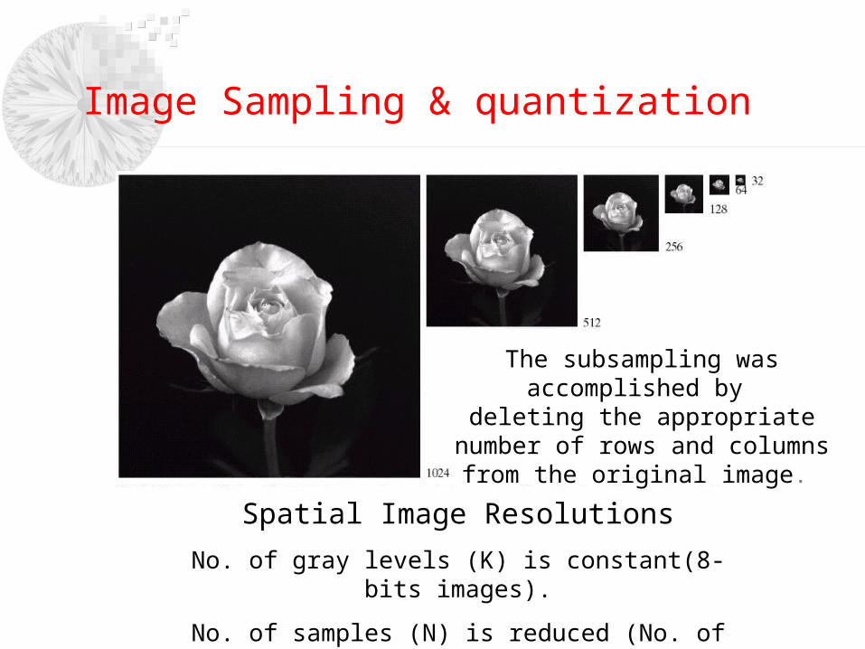
Image Sampling amp quantization
Comparison between all image sizes
Image Sampling amp quantization
Image Sampling amp quantization
Gray Level Image Resolutions
No of samples (N) is constant but gray levels (K) decreases
(false contouring)
Image Sampling amp quantization
Little Intermediate and Large amount of details
What is the effect of changing N and K
Image Sampling amp quantization
Isopreference Curve
Interpolation is the process of using known data to estimate values at unknown locationsInterpolation is a basic tool used in tasks such as zooming shrinking rotating and geometric correctionshrinking and zooming (resampling)
Zooming requires two stepsCreation of a new pixel locationAssignment of a gray level to those new locations
Image Interpolation
Image Interpolation
bull Nearest neighbour interpolation (ex 500 x 500 image)
Laying an imaginary 750 x 750 grid over the original imageShrink it so that it fits exactly over the original imageSpacing in the grid will be less than one pixel Look for the closest pixel in the original image and assign its gray level to the new pixel in the gridFast but produces checkerboard effect
Image Interpolation
Bilinear interpolation (four neighbours of point)Let x y a point in the zoomed image v (x y) a gray level assigned to itv is given by
v (x y) = ax + by + cxy +dThe coefficients are determined from the four equations using the four neighbours
Bicubic interpolation (16 coefficeints)
Better job of preserving finer detailsStandard in commercial image editing programs
3
0
3
0
)(i j
jiij yxayxv
Image Interpolation
Relationship Between Pixels
1- Neighbors of a Pixel
The 4- neighbors of pixel p are
N4(p)
The 4- diagonal neighbors are
ND(p)
The 8-neighbors are
N8(p)
P
P
P
Relationship Between Pixels
Adjacency of Pixels-
Let V be the set of intensity used to define adjacency eg V=1 if we are referring to adjacency of pixels with value 1 in a binary image with 0 and 1In a gray-scale image for the adjacency of pixels with a range of intensity values of say 100 to 120 it follows that V=100101102hellip120We consider three types of adjacency
Adjacency
4- adjacencyTwo pixels p and q with values from V are 4- adjacency if q is in the set N4(p)
Adjacency
8- adjacencyTwo pixels p and q with values from V are 8- adjacency if q is in the set N8(p)
m- adjacency (mixed adjacency)Two pixels p and q with values from V are m- adjacency if
(i) q is in N4(p) or (ii) q is in ND ( p) and N4( p) cap N4 (q) is empty
A (digital) path(or curve) from pixel p at (xy) to pixel q at (st) is a sequence of distinct pixels with coordinates
(x0y0) (x1y1) hellip (xnyn)
where (x0y0) =(xy) (xnyn)=(st) and pixel (xiyi) and (xi-1yi-1) are adjacent for 1le i le n
n is the length of the path
If (x0y0) =(xnyn) the path is a closed path
The path can be defined 4-8-m-paths depending on adjacency type
Path
Connectivity
Let S be a subset of pixels in an image Two pixels p and q are said to be connected in S if there exists a path between them consisting entirely of pixels in SFor any pixel p in S the set of pixels that are connected to it in S is called a connected component of SIf it only has one connected component then set S is called a connected set
Region
Let R be a subset of pixels in an image We call R a region of the image if R is a connected set Two regions are said to be adjacent if their union forms a connected set
Ri Rj are adjacent in 8-adjacency senseThey are not adjacent in 4-adjacency sense
Suppose that an image contains K disjoint regions Rk k = 12 k none of which touches the image border
Let Ru be the union of all the K regions and let (Ru)c denote its complement
We call the points in Ru the foreground and all the points in (Ru)c the background of the imageThe inner boundary (border or contour) of a region R is the set of points that are adjacent to the points in the complement of R ie set of pixels in the region that have at least one background neighbour
Boundary
The point circle is not member of the border of the 1-valued region if 4-connectivity is usedAs a rule adjacency between points in a region and its background is defined in terms of 8-connectivity
Boundary
Boundary
The outer border corresponds to the border in the background This definition to guarantee the existence of a closed path
bull for pixel p q and z with coordinates
(xy) (st) and (uv) respectively
bull D is a distance function or metric if1048708 (a) D(pq) ge 0 D(pq) = 0 iff D=q
1048708 (b) D(pq) = D(qp)
1048708 (c) D(pz) le D(pq) + D(qz)
Distance Measures
1- The Euclidean distance between p and q is defined as
Distance Measures
2- The D4 distance (city-block distance) between p and q is defined as
Distance Measures
3- The D8 distance (chessboard distance) between p and q is defined as
Distance Measures
4- The Dm distance the shortest m-path between the points
Distance Measures
Array product
See matrix multiplication
2221
1211
aa
aa
2221
1211
bb
bb
22222121
12121111
2221
1211
2221
1211
baba
baba
bb
bb
aa
aa
Array Versus Matrix Operations
Linear versus Nonlinear Operations
Consider general operator H
H is said to be a linear operator if
Assume sum operator
)()( yxgyxfH
)()(
)()()()(
yxgayxga
yxfHayxfHayxfayxfaH
jjii
jjiijjii
)()(
)()(
)()()()(
yxgayxga
yxfayxfa
yxfayxfayxfayxfa
jjii
jjii
jjiijjii
Linear versus Nonlinear Operations
Let a1 = 1 a2 =-1
4-
7)1(374
56max)1(
32
20(1)max
2-
42
36max
74
56)1(
32
20)1(max
74
56 and
32
2021
ff
Arithmetic Operations
Carried out between corresponding pixel pairs
Same size of arrays
Let g(xy) denote a corrupted image formed by the addition of noise η(xy) to a noiseless image f(xy)
g(xy) = f(xy) + η(xy)
where the assumption is that at every pair of coordinates (xy) the noise is uncorrelated and has a zero average
)()()(
)()()(
)()()(
)()()(
yxgyxfyxv
yxgyxfyxp
yxgyxfyxd
yxgyxfyxs
Arithmetic Operations
If the noise satisfies the constrains just stated then an image g(xy) is formed by averaging K different noisy images
As K increases the variability of the pixels at each location decreases
)()(
2)(
2)(
1
1
1
)()(
)(1
)(
yxyxg
yxyxg
K
ii
K
K
yxfyxgE
yxgK
yxg
Arithmetic Operations
Arithmetic Operations
Image subtraction is used in the enhancement of the differences between images g(xy) = f(xy) ndash h(xy)
Arithmetic Operations
Application of image multiplication and division is shading correction
If we can get a modeled image as a product of perfect image f(xy) times a shading function h(xy) ie g(xy) = f(xy)h(xy)
If h(xy) is known we can get the perfect image f(xy)
Arithmetic Operations
Multiplication as masking
To solve the range problem in arithmetic operations we can do the following
Given an image f
fm = f ndash min(f) creates an image with min value 0 then
fs = K[fmmax(fm)] creates a scaled image whose range [0 K]
With 8-bit image setting K = 255
Logic Operations
Logic OperationAND p AND q (p q)
OR p OR q (p + q)
COMPLEMENT NOT q ( q )
Logic Operations
Spatial Operations
Performed directly on pixels
Three categoriesSingle-pixel operations
Neighbourhood operations
Geometric spatial transformation
Single-pixel operationsAlter the values of its individual pixels
s = T(z)
Spatial Operations
Neighbourhood operations
Neighbourhood processing generates a corresponding pixel at the same coordinates in an output image
R and c are the row and col Of the pixels whose coordinates are members of the set Sxy
xyScr
crfmn
yxg)(
)(1
)(
Spatial Operations
Geometric spatial transformationModify the spatial relationship between pixels in an image
Consists of two basic operations
Transformation of coordinates Expressed as (xy) = T(vw)
ex (xy) = T(vw) = (v2w2)
Affine transformation (most commonly used)
Scale rotate translate or sheer a set of coordinate points depending on the matrix T
1
0
0
111
3231
2221
1211
tt
tt
tt
wvTwvyx
Spatial Operations
Spatial Operations
The affine equation is used in two ways
Forward mappingScan pixels of the input image
At each location (vw) compute the spatial location (xy)
Two or more pixels in the input image may be transformed to the same location in the output image
Some output locations may not assign a pixel at all
Inverse mapping (more efficient used in commercial MATLAB)Scan the output pixel locations
At each location (xy) compute the spatial location (vw) = T-1(xy)
Interpolate among the nearest input pixels to determine the intensity of the output pixel value
Spatial Operations
Image Registration
Used to align two or more images of the same scene
Input and output images are available but the specific transformation function is not known
Input (image that we wish to transform)
Reference image is the image against which we want to register the input
One approach is using tie points (control points)
The location of the points are precisely known in input and reference images
Using the bilinear approximation is a simple model and given by
x = c1v+c2w+c3vw+c4
y = c5v+c6w+c7vw+c8
(xy) ndash reference image (vw) ndash input image tie points
Image Registration
Four pairs of the corresponding points -gt 8 equations to find the unknown coefficients
Image Transformation
A 2-D transform denoted T(uv) can be expressed in the general form
r(xyuv) forward transformation kernel
s(xyuv) inverse transformation kernel
1
0
1
0
)()()(M
x
N
y
vuyxryxfvuT
1
0
1
0
)()()(M
u
N
v
vuyxsvuTyxf
Image Transformation
Image Transformation
The forward transformation kernel is said to be separable if
kernel is said to be symmetric if r1(xy) is functionally equal to r2(xy) so that
2-D Fourier transform
)()()( 21 vyruxrvuyxr
)()()( 11 vyruxrvuyxr
1
0
1
0
)(2)()(M
x
N
y
NvyMuxjeyxfvuT
1
0
1
0
)(2)(1
)(M
u
N
v
NvyMuxjevuTMN
yxf
Probabilistic Methods
Treating intensities as random quantities is the simplest way of applying probability to image processing
Let zi i=012hellipL-1 possible intensities
Then the probability P(zk ) of intensity level zk is
So
Is the measure of the spread of the value of z about the mean so it is useful to measure an image contrast
MN
nzp k
k )(
1
0
22
1
0
1
0
)()(
)(
1)(
L
kkk
L
kkk
L
kk
zpmz
zpzmaveragemean
zp
Probabilistic Methods
Standard deviation is 143 316 492 intensity level
The variance is 2043 9978 24249
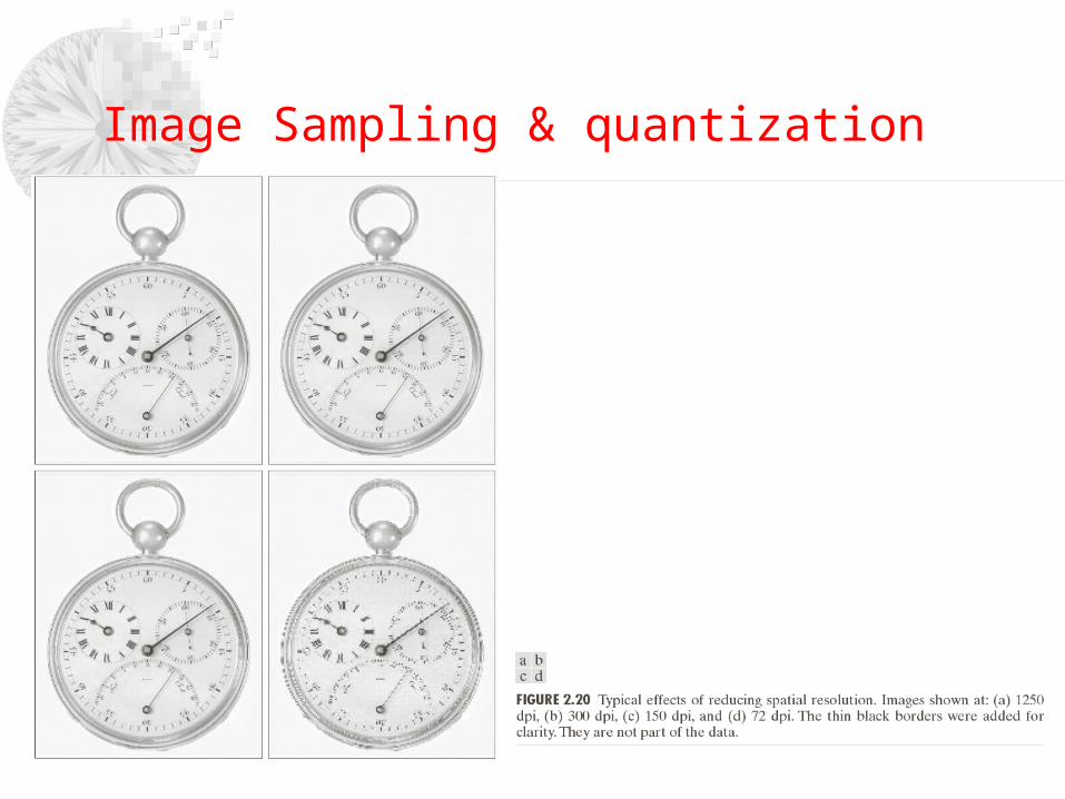
Image Sampling amp quantization
Image Sampling amp quantization
Gray Level Image Resolutions
No of samples (N) is constant but gray levels (K) decreases
(false contouring)
Image Sampling amp quantization
Little Intermediate and Large amount of details
What is the effect of changing N and K
Image Sampling amp quantization
Isopreference Curve
Interpolation is the process of using known data to estimate values at unknown locationsInterpolation is a basic tool used in tasks such as zooming shrinking rotating and geometric correctionshrinking and zooming (resampling)
Zooming requires two stepsCreation of a new pixel locationAssignment of a gray level to those new locations
Image Interpolation
Image Interpolation
bull Nearest neighbour interpolation (ex 500 x 500 image)
Laying an imaginary 750 x 750 grid over the original imageShrink it so that it fits exactly over the original imageSpacing in the grid will be less than one pixel Look for the closest pixel in the original image and assign its gray level to the new pixel in the gridFast but produces checkerboard effect
Image Interpolation
Bilinear interpolation (four neighbours of point)Let x y a point in the zoomed image v (x y) a gray level assigned to itv is given by
v (x y) = ax + by + cxy +dThe coefficients are determined from the four equations using the four neighbours
Bicubic interpolation (16 coefficeints)
Better job of preserving finer detailsStandard in commercial image editing programs
3
0
3
0
)(i j
jiij yxayxv
Image Interpolation
Relationship Between Pixels
1- Neighbors of a Pixel
The 4- neighbors of pixel p are
N4(p)
The 4- diagonal neighbors are
ND(p)
The 8-neighbors are
N8(p)
P
P
P
Relationship Between Pixels
Adjacency of Pixels-
Let V be the set of intensity used to define adjacency eg V=1 if we are referring to adjacency of pixels with value 1 in a binary image with 0 and 1In a gray-scale image for the adjacency of pixels with a range of intensity values of say 100 to 120 it follows that V=100101102hellip120We consider three types of adjacency
Adjacency
4- adjacencyTwo pixels p and q with values from V are 4- adjacency if q is in the set N4(p)
Adjacency
8- adjacencyTwo pixels p and q with values from V are 8- adjacency if q is in the set N8(p)
m- adjacency (mixed adjacency)Two pixels p and q with values from V are m- adjacency if
(i) q is in N4(p) or (ii) q is in ND ( p) and N4( p) cap N4 (q) is empty
A (digital) path(or curve) from pixel p at (xy) to pixel q at (st) is a sequence of distinct pixels with coordinates
(x0y0) (x1y1) hellip (xnyn)
where (x0y0) =(xy) (xnyn)=(st) and pixel (xiyi) and (xi-1yi-1) are adjacent for 1le i le n
n is the length of the path
If (x0y0) =(xnyn) the path is a closed path
The path can be defined 4-8-m-paths depending on adjacency type
Path
Connectivity
Let S be a subset of pixels in an image Two pixels p and q are said to be connected in S if there exists a path between them consisting entirely of pixels in SFor any pixel p in S the set of pixels that are connected to it in S is called a connected component of SIf it only has one connected component then set S is called a connected set
Region
Let R be a subset of pixels in an image We call R a region of the image if R is a connected set Two regions are said to be adjacent if their union forms a connected set
Ri Rj are adjacent in 8-adjacency senseThey are not adjacent in 4-adjacency sense
Suppose that an image contains K disjoint regions Rk k = 12 k none of which touches the image border
Let Ru be the union of all the K regions and let (Ru)c denote its complement
We call the points in Ru the foreground and all the points in (Ru)c the background of the imageThe inner boundary (border or contour) of a region R is the set of points that are adjacent to the points in the complement of R ie set of pixels in the region that have at least one background neighbour
Boundary
The point circle is not member of the border of the 1-valued region if 4-connectivity is usedAs a rule adjacency between points in a region and its background is defined in terms of 8-connectivity
Boundary
Boundary
The outer border corresponds to the border in the background This definition to guarantee the existence of a closed path
bull for pixel p q and z with coordinates
(xy) (st) and (uv) respectively
bull D is a distance function or metric if1048708 (a) D(pq) ge 0 D(pq) = 0 iff D=q
1048708 (b) D(pq) = D(qp)
1048708 (c) D(pz) le D(pq) + D(qz)
Distance Measures
1- The Euclidean distance between p and q is defined as
Distance Measures
2- The D4 distance (city-block distance) between p and q is defined as
Distance Measures
3- The D8 distance (chessboard distance) between p and q is defined as
Distance Measures
4- The Dm distance the shortest m-path between the points
Distance Measures
Array product
See matrix multiplication
2221
1211
aa
aa
2221
1211
bb
bb
22222121
12121111
2221
1211
2221
1211
baba
baba
bb
bb
aa
aa
Array Versus Matrix Operations
Linear versus Nonlinear Operations
Consider general operator H
H is said to be a linear operator if
Assume sum operator
)()( yxgyxfH
)()(
)()()()(
yxgayxga
yxfHayxfHayxfayxfaH
jjii
jjiijjii
)()(
)()(
)()()()(
yxgayxga
yxfayxfa
yxfayxfayxfayxfa
jjii
jjii
jjiijjii
Linear versus Nonlinear Operations
Let a1 = 1 a2 =-1
4-
7)1(374
56max)1(
32
20(1)max
2-
42
36max
74
56)1(
32
20)1(max
74
56 and
32
2021
ff
Arithmetic Operations
Carried out between corresponding pixel pairs
Same size of arrays
Let g(xy) denote a corrupted image formed by the addition of noise η(xy) to a noiseless image f(xy)
g(xy) = f(xy) + η(xy)
where the assumption is that at every pair of coordinates (xy) the noise is uncorrelated and has a zero average
)()()(
)()()(
)()()(
)()()(
yxgyxfyxv
yxgyxfyxp
yxgyxfyxd
yxgyxfyxs
Arithmetic Operations
If the noise satisfies the constrains just stated then an image g(xy) is formed by averaging K different noisy images
As K increases the variability of the pixels at each location decreases
)()(
2)(
2)(
1
1
1
)()(
)(1
)(
yxyxg
yxyxg
K
ii
K
K
yxfyxgE
yxgK
yxg
Arithmetic Operations
Arithmetic Operations
Image subtraction is used in the enhancement of the differences between images g(xy) = f(xy) ndash h(xy)
Arithmetic Operations
Application of image multiplication and division is shading correction
If we can get a modeled image as a product of perfect image f(xy) times a shading function h(xy) ie g(xy) = f(xy)h(xy)
If h(xy) is known we can get the perfect image f(xy)
Arithmetic Operations
Multiplication as masking
To solve the range problem in arithmetic operations we can do the following
Given an image f
fm = f ndash min(f) creates an image with min value 0 then
fs = K[fmmax(fm)] creates a scaled image whose range [0 K]
With 8-bit image setting K = 255
Logic Operations
Logic OperationAND p AND q (p q)
OR p OR q (p + q)
COMPLEMENT NOT q ( q )
Logic Operations
Spatial Operations
Performed directly on pixels
Three categoriesSingle-pixel operations
Neighbourhood operations
Geometric spatial transformation
Single-pixel operationsAlter the values of its individual pixels
s = T(z)
Spatial Operations
Neighbourhood operations
Neighbourhood processing generates a corresponding pixel at the same coordinates in an output image
R and c are the row and col Of the pixels whose coordinates are members of the set Sxy
xyScr
crfmn
yxg)(
)(1
)(
Spatial Operations
Geometric spatial transformationModify the spatial relationship between pixels in an image
Consists of two basic operations
Transformation of coordinates Expressed as (xy) = T(vw)
ex (xy) = T(vw) = (v2w2)
Affine transformation (most commonly used)
Scale rotate translate or sheer a set of coordinate points depending on the matrix T
1
0
0
111
3231
2221
1211
tt
tt
tt
wvTwvyx
Spatial Operations
Spatial Operations
The affine equation is used in two ways
Forward mappingScan pixels of the input image
At each location (vw) compute the spatial location (xy)
Two or more pixels in the input image may be transformed to the same location in the output image
Some output locations may not assign a pixel at all
Inverse mapping (more efficient used in commercial MATLAB)Scan the output pixel locations
At each location (xy) compute the spatial location (vw) = T-1(xy)
Interpolate among the nearest input pixels to determine the intensity of the output pixel value
Spatial Operations
Image Registration
Used to align two or more images of the same scene
Input and output images are available but the specific transformation function is not known
Input (image that we wish to transform)
Reference image is the image against which we want to register the input
One approach is using tie points (control points)
The location of the points are precisely known in input and reference images
Using the bilinear approximation is a simple model and given by
x = c1v+c2w+c3vw+c4
y = c5v+c6w+c7vw+c8
(xy) ndash reference image (vw) ndash input image tie points
Image Registration
Four pairs of the corresponding points -gt 8 equations to find the unknown coefficients
Image Transformation
A 2-D transform denoted T(uv) can be expressed in the general form
r(xyuv) forward transformation kernel
s(xyuv) inverse transformation kernel
1
0
1
0
)()()(M
x
N
y
vuyxryxfvuT
1
0
1
0
)()()(M
u
N
v
vuyxsvuTyxf
Image Transformation
Image Transformation
The forward transformation kernel is said to be separable if
kernel is said to be symmetric if r1(xy) is functionally equal to r2(xy) so that
2-D Fourier transform
)()()( 21 vyruxrvuyxr
)()()( 11 vyruxrvuyxr
1
0
1
0
)(2)()(M
x
N
y
NvyMuxjeyxfvuT
1
0
1
0
)(2)(1
)(M
u
N
v
NvyMuxjevuTMN
yxf
Probabilistic Methods
Treating intensities as random quantities is the simplest way of applying probability to image processing
Let zi i=012hellipL-1 possible intensities
Then the probability P(zk ) of intensity level zk is
So
Is the measure of the spread of the value of z about the mean so it is useful to measure an image contrast
MN
nzp k
k )(
1
0
22
1
0
1
0
)()(
)(
1)(
L
kkk
L
kkk
L
kk
zpmz
zpzmaveragemean
zp
Probabilistic Methods
Standard deviation is 143 316 492 intensity level
The variance is 2043 9978 24249
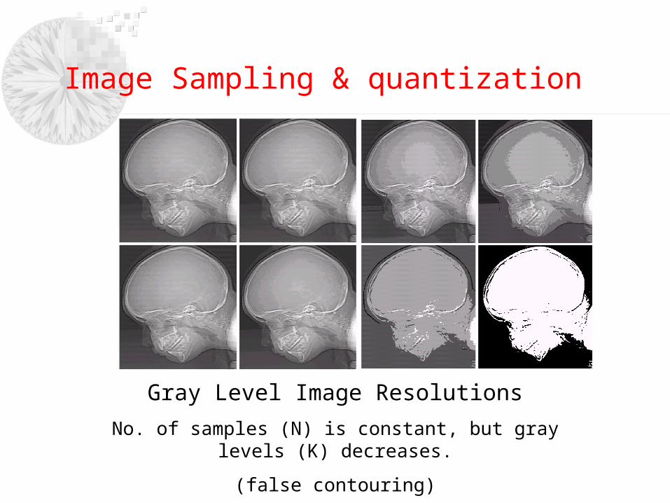
Image Sampling amp quantization
Isopreference Curve
Interpolation is the process of using known data to estimate values at unknown locationsInterpolation is a basic tool used in tasks such as zooming shrinking rotating and geometric correctionshrinking and zooming (resampling)
Zooming requires two stepsCreation of a new pixel locationAssignment of a gray level to those new locations
Image Interpolation
Image Interpolation
bull Nearest neighbour interpolation (ex 500 x 500 image)
Laying an imaginary 750 x 750 grid over the original imageShrink it so that it fits exactly over the original imageSpacing in the grid will be less than one pixel Look for the closest pixel in the original image and assign its gray level to the new pixel in the gridFast but produces checkerboard effect
Image Interpolation
Bilinear interpolation (four neighbours of point)Let x y a point in the zoomed image v (x y) a gray level assigned to itv is given by
v (x y) = ax + by + cxy +dThe coefficients are determined from the four equations using the four neighbours
Bicubic interpolation (16 coefficeints)
Better job of preserving finer detailsStandard in commercial image editing programs
3
0
3
0
)(i j
jiij yxayxv
Image Interpolation
Relationship Between Pixels
1- Neighbors of a Pixel
The 4- neighbors of pixel p are
N4(p)
The 4- diagonal neighbors are
ND(p)
The 8-neighbors are
N8(p)
P
P
P
Relationship Between Pixels
Adjacency of Pixels-
Let V be the set of intensity used to define adjacency eg V=1 if we are referring to adjacency of pixels with value 1 in a binary image with 0 and 1In a gray-scale image for the adjacency of pixels with a range of intensity values of say 100 to 120 it follows that V=100101102hellip120We consider three types of adjacency
Adjacency
4- adjacencyTwo pixels p and q with values from V are 4- adjacency if q is in the set N4(p)
Adjacency
8- adjacencyTwo pixels p and q with values from V are 8- adjacency if q is in the set N8(p)
m- adjacency (mixed adjacency)Two pixels p and q with values from V are m- adjacency if
(i) q is in N4(p) or (ii) q is in ND ( p) and N4( p) cap N4 (q) is empty
A (digital) path(or curve) from pixel p at (xy) to pixel q at (st) is a sequence of distinct pixels with coordinates
(x0y0) (x1y1) hellip (xnyn)
where (x0y0) =(xy) (xnyn)=(st) and pixel (xiyi) and (xi-1yi-1) are adjacent for 1le i le n
n is the length of the path
If (x0y0) =(xnyn) the path is a closed path
The path can be defined 4-8-m-paths depending on adjacency type
Path
Connectivity
Let S be a subset of pixels in an image Two pixels p and q are said to be connected in S if there exists a path between them consisting entirely of pixels in SFor any pixel p in S the set of pixels that are connected to it in S is called a connected component of SIf it only has one connected component then set S is called a connected set
Region
Let R be a subset of pixels in an image We call R a region of the image if R is a connected set Two regions are said to be adjacent if their union forms a connected set
Ri Rj are adjacent in 8-adjacency senseThey are not adjacent in 4-adjacency sense
Suppose that an image contains K disjoint regions Rk k = 12 k none of which touches the image border
Let Ru be the union of all the K regions and let (Ru)c denote its complement
We call the points in Ru the foreground and all the points in (Ru)c the background of the imageThe inner boundary (border or contour) of a region R is the set of points that are adjacent to the points in the complement of R ie set of pixels in the region that have at least one background neighbour
Boundary
The point circle is not member of the border of the 1-valued region if 4-connectivity is usedAs a rule adjacency between points in a region and its background is defined in terms of 8-connectivity
Boundary
Boundary
The outer border corresponds to the border in the background This definition to guarantee the existence of a closed path
bull for pixel p q and z with coordinates
(xy) (st) and (uv) respectively
bull D is a distance function or metric if1048708 (a) D(pq) ge 0 D(pq) = 0 iff D=q
1048708 (b) D(pq) = D(qp)
1048708 (c) D(pz) le D(pq) + D(qz)
Distance Measures
1- The Euclidean distance between p and q is defined as
Distance Measures
2- The D4 distance (city-block distance) between p and q is defined as
Distance Measures
3- The D8 distance (chessboard distance) between p and q is defined as
Distance Measures
4- The Dm distance the shortest m-path between the points
Distance Measures
Array product
See matrix multiplication
2221
1211
aa
aa
2221
1211
bb
bb
22222121
12121111
2221
1211
2221
1211
baba
baba
bb
bb
aa
aa
Array Versus Matrix Operations
Linear versus Nonlinear Operations
Consider general operator H
H is said to be a linear operator if
Assume sum operator
)()( yxgyxfH
)()(
)()()()(
yxgayxga
yxfHayxfHayxfayxfaH
jjii
jjiijjii
)()(
)()(
)()()()(
yxgayxga
yxfayxfa
yxfayxfayxfayxfa
jjii
jjii
jjiijjii
Linear versus Nonlinear Operations
Let a1 = 1 a2 =-1
4-
7)1(374
56max)1(
32
20(1)max
2-
42
36max
74
56)1(
32
20)1(max
74
56 and
32
2021
ff
Arithmetic Operations
Carried out between corresponding pixel pairs
Same size of arrays
Let g(xy) denote a corrupted image formed by the addition of noise η(xy) to a noiseless image f(xy)
g(xy) = f(xy) + η(xy)
where the assumption is that at every pair of coordinates (xy) the noise is uncorrelated and has a zero average
)()()(
)()()(
)()()(
)()()(
yxgyxfyxv
yxgyxfyxp
yxgyxfyxd
yxgyxfyxs
Arithmetic Operations
If the noise satisfies the constrains just stated then an image g(xy) is formed by averaging K different noisy images
As K increases the variability of the pixels at each location decreases
)()(
2)(
2)(
1
1
1
)()(
)(1
)(
yxyxg
yxyxg
K
ii
K
K
yxfyxgE
yxgK
yxg
Arithmetic Operations
Arithmetic Operations
Image subtraction is used in the enhancement of the differences between images g(xy) = f(xy) ndash h(xy)
Arithmetic Operations
Application of image multiplication and division is shading correction
If we can get a modeled image as a product of perfect image f(xy) times a shading function h(xy) ie g(xy) = f(xy)h(xy)
If h(xy) is known we can get the perfect image f(xy)
Arithmetic Operations
Multiplication as masking
To solve the range problem in arithmetic operations we can do the following
Given an image f
fm = f ndash min(f) creates an image with min value 0 then
fs = K[fmmax(fm)] creates a scaled image whose range [0 K]
With 8-bit image setting K = 255
Logic Operations
Logic OperationAND p AND q (p q)
OR p OR q (p + q)
COMPLEMENT NOT q ( q )
Logic Operations
Spatial Operations
Performed directly on pixels
Three categoriesSingle-pixel operations
Neighbourhood operations
Geometric spatial transformation
Single-pixel operationsAlter the values of its individual pixels
s = T(z)
Spatial Operations
Neighbourhood operations
Neighbourhood processing generates a corresponding pixel at the same coordinates in an output image
R and c are the row and col Of the pixels whose coordinates are members of the set Sxy
xyScr
crfmn
yxg)(
)(1
)(
Spatial Operations
Geometric spatial transformationModify the spatial relationship between pixels in an image
Consists of two basic operations
Transformation of coordinates Expressed as (xy) = T(vw)
ex (xy) = T(vw) = (v2w2)
Affine transformation (most commonly used)
Scale rotate translate or sheer a set of coordinate points depending on the matrix T
1
0
0
111
3231
2221
1211
tt
tt
tt
wvTwvyx
Spatial Operations
Spatial Operations
The affine equation is used in two ways
Forward mappingScan pixels of the input image
At each location (vw) compute the spatial location (xy)
Two or more pixels in the input image may be transformed to the same location in the output image
Some output locations may not assign a pixel at all
Inverse mapping (more efficient used in commercial MATLAB)Scan the output pixel locations
At each location (xy) compute the spatial location (vw) = T-1(xy)
Interpolate among the nearest input pixels to determine the intensity of the output pixel value
Spatial Operations
Image Registration
Used to align two or more images of the same scene
Input and output images are available but the specific transformation function is not known
Input (image that we wish to transform)
Reference image is the image against which we want to register the input
One approach is using tie points (control points)
The location of the points are precisely known in input and reference images
Using the bilinear approximation is a simple model and given by
x = c1v+c2w+c3vw+c4
y = c5v+c6w+c7vw+c8
(xy) ndash reference image (vw) ndash input image tie points
Image Registration
Four pairs of the corresponding points -gt 8 equations to find the unknown coefficients
Image Transformation
A 2-D transform denoted T(uv) can be expressed in the general form
r(xyuv) forward transformation kernel
s(xyuv) inverse transformation kernel
1
0
1
0
)()()(M
x
N
y
vuyxryxfvuT
1
0
1
0
)()()(M
u
N
v
vuyxsvuTyxf
Image Transformation
Image Transformation
The forward transformation kernel is said to be separable if
kernel is said to be symmetric if r1(xy) is functionally equal to r2(xy) so that
2-D Fourier transform
)()()( 21 vyruxrvuyxr
)()()( 11 vyruxrvuyxr
1
0
1
0
)(2)()(M
x
N
y
NvyMuxjeyxfvuT
1
0
1
0
)(2)(1
)(M
u
N
v
NvyMuxjevuTMN
yxf
Probabilistic Methods
Treating intensities as random quantities is the simplest way of applying probability to image processing
Let zi i=012hellipL-1 possible intensities
Then the probability P(zk ) of intensity level zk is
So
Is the measure of the spread of the value of z about the mean so it is useful to measure an image contrast
MN
nzp k
k )(
1
0
22
1
0
1
0
)()(
)(
1)(
L
kkk
L
kkk
L
kk
zpmz
zpzmaveragemean
zp
Probabilistic Methods
Standard deviation is 143 316 492 intensity level
The variance is 2043 9978 24249
Image Interpolation
bull Nearest neighbour interpolation (ex 500 x 500 image)
Laying an imaginary 750 x 750 grid over the original imageShrink it so that it fits exactly over the original imageSpacing in the grid will be less than one pixel Look for the closest pixel in the original image and assign its gray level to the new pixel in the gridFast but produces checkerboard effect
Image Interpolation
Bilinear interpolation (four neighbours of point)Let x y a point in the zoomed image v (x y) a gray level assigned to itv is given by
v (x y) = ax + by + cxy +dThe coefficients are determined from the four equations using the four neighbours
Bicubic interpolation (16 coefficeints)
Better job of preserving finer detailsStandard in commercial image editing programs
3
0
3
0
)(i j
jiij yxayxv
Image Interpolation
Relationship Between Pixels
1- Neighbors of a Pixel
The 4- neighbors of pixel p are
N4(p)
The 4- diagonal neighbors are
ND(p)
The 8-neighbors are
N8(p)
P
P
P
Relationship Between Pixels
Adjacency of Pixels-
Let V be the set of intensity used to define adjacency eg V=1 if we are referring to adjacency of pixels with value 1 in a binary image with 0 and 1In a gray-scale image for the adjacency of pixels with a range of intensity values of say 100 to 120 it follows that V=100101102hellip120We consider three types of adjacency
Adjacency
4- adjacencyTwo pixels p and q with values from V are 4- adjacency if q is in the set N4(p)
Adjacency
8- adjacencyTwo pixels p and q with values from V are 8- adjacency if q is in the set N8(p)
m- adjacency (mixed adjacency)Two pixels p and q with values from V are m- adjacency if
(i) q is in N4(p) or (ii) q is in ND ( p) and N4( p) cap N4 (q) is empty
A (digital) path(or curve) from pixel p at (xy) to pixel q at (st) is a sequence of distinct pixels with coordinates
(x0y0) (x1y1) hellip (xnyn)
where (x0y0) =(xy) (xnyn)=(st) and pixel (xiyi) and (xi-1yi-1) are adjacent for 1le i le n
n is the length of the path
If (x0y0) =(xnyn) the path is a closed path
The path can be defined 4-8-m-paths depending on adjacency type
Path
Connectivity
Let S be a subset of pixels in an image Two pixels p and q are said to be connected in S if there exists a path between them consisting entirely of pixels in SFor any pixel p in S the set of pixels that are connected to it in S is called a connected component of SIf it only has one connected component then set S is called a connected set
Region
Let R be a subset of pixels in an image We call R a region of the image if R is a connected set Two regions are said to be adjacent if their union forms a connected set
Ri Rj are adjacent in 8-adjacency senseThey are not adjacent in 4-adjacency sense
Suppose that an image contains K disjoint regions Rk k = 12 k none of which touches the image border
Let Ru be the union of all the K regions and let (Ru)c denote its complement
We call the points in Ru the foreground and all the points in (Ru)c the background of the imageThe inner boundary (border or contour) of a region R is the set of points that are adjacent to the points in the complement of R ie set of pixels in the region that have at least one background neighbour
Boundary
The point circle is not member of the border of the 1-valued region if 4-connectivity is usedAs a rule adjacency between points in a region and its background is defined in terms of 8-connectivity
Boundary
Boundary
The outer border corresponds to the border in the background This definition to guarantee the existence of a closed path
bull for pixel p q and z with coordinates
(xy) (st) and (uv) respectively
bull D is a distance function or metric if1048708 (a) D(pq) ge 0 D(pq) = 0 iff D=q
1048708 (b) D(pq) = D(qp)
1048708 (c) D(pz) le D(pq) + D(qz)
Distance Measures
1- The Euclidean distance between p and q is defined as
Distance Measures
2- The D4 distance (city-block distance) between p and q is defined as
Distance Measures
3- The D8 distance (chessboard distance) between p and q is defined as
Distance Measures
4- The Dm distance the shortest m-path between the points
Distance Measures
Array product
See matrix multiplication
2221
1211
aa
aa
2221
1211
bb
bb
22222121
12121111
2221
1211
2221
1211
baba
baba
bb
bb
aa
aa
Array Versus Matrix Operations
Linear versus Nonlinear Operations
Consider general operator H
H is said to be a linear operator if
Assume sum operator
)()( yxgyxfH
)()(
)()()()(
yxgayxga
yxfHayxfHayxfayxfaH
jjii
jjiijjii
)()(
)()(
)()()()(
yxgayxga
yxfayxfa
yxfayxfayxfayxfa
jjii
jjii
jjiijjii
Linear versus Nonlinear Operations
Let a1 = 1 a2 =-1
4-
7)1(374
56max)1(
32
20(1)max
2-
42
36max
74
56)1(
32
20)1(max
74
56 and
32
2021
ff
Arithmetic Operations
Carried out between corresponding pixel pairs
Same size of arrays
Let g(xy) denote a corrupted image formed by the addition of noise η(xy) to a noiseless image f(xy)
g(xy) = f(xy) + η(xy)
where the assumption is that at every pair of coordinates (xy) the noise is uncorrelated and has a zero average
)()()(
)()()(
)()()(
)()()(
yxgyxfyxv
yxgyxfyxp
yxgyxfyxd
yxgyxfyxs
Arithmetic Operations
If the noise satisfies the constrains just stated then an image g(xy) is formed by averaging K different noisy images
As K increases the variability of the pixels at each location decreases
)()(
2)(
2)(
1
1
1
)()(
)(1
)(
yxyxg
yxyxg
K
ii
K
K
yxfyxgE
yxgK
yxg
Arithmetic Operations
Arithmetic Operations
Image subtraction is used in the enhancement of the differences between images g(xy) = f(xy) ndash h(xy)
Arithmetic Operations
Application of image multiplication and division is shading correction
If we can get a modeled image as a product of perfect image f(xy) times a shading function h(xy) ie g(xy) = f(xy)h(xy)
If h(xy) is known we can get the perfect image f(xy)
Arithmetic Operations
Multiplication as masking
To solve the range problem in arithmetic operations we can do the following
Given an image f
fm = f ndash min(f) creates an image with min value 0 then
fs = K[fmmax(fm)] creates a scaled image whose range [0 K]
With 8-bit image setting K = 255
Logic Operations
Logic OperationAND p AND q (p q)
OR p OR q (p + q)
COMPLEMENT NOT q ( q )
Logic Operations
Spatial Operations
Performed directly on pixels
Three categoriesSingle-pixel operations
Neighbourhood operations
Geometric spatial transformation
Single-pixel operationsAlter the values of its individual pixels
s = T(z)
Spatial Operations
Neighbourhood operations
Neighbourhood processing generates a corresponding pixel at the same coordinates in an output image
R and c are the row and col Of the pixels whose coordinates are members of the set Sxy
xyScr
crfmn
yxg)(
)(1
)(
Spatial Operations
Geometric spatial transformationModify the spatial relationship between pixels in an image
Consists of two basic operations
Transformation of coordinates Expressed as (xy) = T(vw)
ex (xy) = T(vw) = (v2w2)
Affine transformation (most commonly used)
Scale rotate translate or sheer a set of coordinate points depending on the matrix T
1
0
0
111
3231
2221
1211
tt
tt
tt
wvTwvyx
Spatial Operations
Spatial Operations
The affine equation is used in two ways
Forward mappingScan pixels of the input image
At each location (vw) compute the spatial location (xy)
Two or more pixels in the input image may be transformed to the same location in the output image
Some output locations may not assign a pixel at all
Inverse mapping (more efficient used in commercial MATLAB)Scan the output pixel locations
At each location (xy) compute the spatial location (vw) = T-1(xy)
Interpolate among the nearest input pixels to determine the intensity of the output pixel value
Spatial Operations
Image Registration
Used to align two or more images of the same scene
Input and output images are available but the specific transformation function is not known
Input (image that we wish to transform)
Reference image is the image against which we want to register the input
One approach is using tie points (control points)
The location of the points are precisely known in input and reference images
Using the bilinear approximation is a simple model and given by
x = c1v+c2w+c3vw+c4
y = c5v+c6w+c7vw+c8
(xy) ndash reference image (vw) ndash input image tie points
Image Registration
Four pairs of the corresponding points -gt 8 equations to find the unknown coefficients
Image Transformation
A 2-D transform denoted T(uv) can be expressed in the general form
r(xyuv) forward transformation kernel
s(xyuv) inverse transformation kernel
1
0
1
0
)()()(M
x
N
y
vuyxryxfvuT
1
0
1
0
)()()(M
u
N
v
vuyxsvuTyxf
Image Transformation
Image Transformation
The forward transformation kernel is said to be separable if
kernel is said to be symmetric if r1(xy) is functionally equal to r2(xy) so that
2-D Fourier transform
)()()( 21 vyruxrvuyxr
)()()( 11 vyruxrvuyxr
1
0
1
0
)(2)()(M
x
N
y
NvyMuxjeyxfvuT
1
0
1
0
)(2)(1
)(M
u
N
v
NvyMuxjevuTMN
yxf
Probabilistic Methods
Treating intensities as random quantities is the simplest way of applying probability to image processing
Let zi i=012hellipL-1 possible intensities
Then the probability P(zk ) of intensity level zk is
So
Is the measure of the spread of the value of z about the mean so it is useful to measure an image contrast
MN
nzp k
k )(
1
0
22
1
0
1
0
)()(
)(
1)(
L
kkk
L
kkk
L
kk
zpmz
zpzmaveragemean
zp
Probabilistic Methods
Standard deviation is 143 316 492 intensity level
The variance is 2043 9978 24249

Image Interpolation
Relationship Between Pixels
1- Neighbors of a Pixel
The 4- neighbors of pixel p are
N4(p)
The 4- diagonal neighbors are
ND(p)
The 8-neighbors are
N8(p)
P
P
P
Relationship Between Pixels
Adjacency of Pixels-
Let V be the set of intensity used to define adjacency eg V=1 if we are referring to adjacency of pixels with value 1 in a binary image with 0 and 1In a gray-scale image for the adjacency of pixels with a range of intensity values of say 100 to 120 it follows that V=100101102hellip120We consider three types of adjacency
Adjacency
4- adjacencyTwo pixels p and q with values from V are 4- adjacency if q is in the set N4(p)
Adjacency
8- adjacencyTwo pixels p and q with values from V are 8- adjacency if q is in the set N8(p)
m- adjacency (mixed adjacency)Two pixels p and q with values from V are m- adjacency if
(i) q is in N4(p) or (ii) q is in ND ( p) and N4( p) cap N4 (q) is empty
A (digital) path(or curve) from pixel p at (xy) to pixel q at (st) is a sequence of distinct pixels with coordinates
(x0y0) (x1y1) hellip (xnyn)
where (x0y0) =(xy) (xnyn)=(st) and pixel (xiyi) and (xi-1yi-1) are adjacent for 1le i le n
n is the length of the path
If (x0y0) =(xnyn) the path is a closed path
The path can be defined 4-8-m-paths depending on adjacency type
Path
Connectivity
Let S be a subset of pixels in an image Two pixels p and q are said to be connected in S if there exists a path between them consisting entirely of pixels in SFor any pixel p in S the set of pixels that are connected to it in S is called a connected component of SIf it only has one connected component then set S is called a connected set
Region
Let R be a subset of pixels in an image We call R a region of the image if R is a connected set Two regions are said to be adjacent if their union forms a connected set
Ri Rj are adjacent in 8-adjacency senseThey are not adjacent in 4-adjacency sense
Suppose that an image contains K disjoint regions Rk k = 12 k none of which touches the image border
Let Ru be the union of all the K regions and let (Ru)c denote its complement
We call the points in Ru the foreground and all the points in (Ru)c the background of the imageThe inner boundary (border or contour) of a region R is the set of points that are adjacent to the points in the complement of R ie set of pixels in the region that have at least one background neighbour
Boundary
The point circle is not member of the border of the 1-valued region if 4-connectivity is usedAs a rule adjacency between points in a region and its background is defined in terms of 8-connectivity
Boundary
Boundary
The outer border corresponds to the border in the background This definition to guarantee the existence of a closed path
bull for pixel p q and z with coordinates
(xy) (st) and (uv) respectively
bull D is a distance function or metric if1048708 (a) D(pq) ge 0 D(pq) = 0 iff D=q
1048708 (b) D(pq) = D(qp)
1048708 (c) D(pz) le D(pq) + D(qz)
Distance Measures
1- The Euclidean distance between p and q is defined as
Distance Measures
2- The D4 distance (city-block distance) between p and q is defined as
Distance Measures
3- The D8 distance (chessboard distance) between p and q is defined as
Distance Measures
4- The Dm distance the shortest m-path between the points
Distance Measures
Array product
See matrix multiplication
2221
1211
aa
aa
2221
1211
bb
bb
22222121
12121111
2221
1211
2221
1211
baba
baba
bb
bb
aa
aa
Array Versus Matrix Operations
Linear versus Nonlinear Operations
Consider general operator H
H is said to be a linear operator if
Assume sum operator
)()( yxgyxfH
)()(
)()()()(
yxgayxga
yxfHayxfHayxfayxfaH
jjii
jjiijjii
)()(
)()(
)()()()(
yxgayxga
yxfayxfa
yxfayxfayxfayxfa
jjii
jjii
jjiijjii
Linear versus Nonlinear Operations
Let a1 = 1 a2 =-1
4-
7)1(374
56max)1(
32
20(1)max
2-
42
36max
74
56)1(
32
20)1(max
74
56 and
32
2021
ff
Arithmetic Operations
Carried out between corresponding pixel pairs
Same size of arrays
Let g(xy) denote a corrupted image formed by the addition of noise η(xy) to a noiseless image f(xy)
g(xy) = f(xy) + η(xy)
where the assumption is that at every pair of coordinates (xy) the noise is uncorrelated and has a zero average
)()()(
)()()(
)()()(
)()()(
yxgyxfyxv
yxgyxfyxp
yxgyxfyxd
yxgyxfyxs
Arithmetic Operations
If the noise satisfies the constrains just stated then an image g(xy) is formed by averaging K different noisy images
As K increases the variability of the pixels at each location decreases
)()(
2)(
2)(
1
1
1
)()(
)(1
)(
yxyxg
yxyxg
K
ii
K
K
yxfyxgE
yxgK
yxg
Arithmetic Operations
Arithmetic Operations
Image subtraction is used in the enhancement of the differences between images g(xy) = f(xy) ndash h(xy)
Arithmetic Operations
Application of image multiplication and division is shading correction
If we can get a modeled image as a product of perfect image f(xy) times a shading function h(xy) ie g(xy) = f(xy)h(xy)
If h(xy) is known we can get the perfect image f(xy)
Arithmetic Operations
Multiplication as masking
To solve the range problem in arithmetic operations we can do the following
Given an image f
fm = f ndash min(f) creates an image with min value 0 then
fs = K[fmmax(fm)] creates a scaled image whose range [0 K]
With 8-bit image setting K = 255
Logic Operations
Logic OperationAND p AND q (p q)
OR p OR q (p + q)
COMPLEMENT NOT q ( q )
Logic Operations
Spatial Operations
Performed directly on pixels
Three categoriesSingle-pixel operations
Neighbourhood operations
Geometric spatial transformation
Single-pixel operationsAlter the values of its individual pixels
s = T(z)
Spatial Operations
Neighbourhood operations
Neighbourhood processing generates a corresponding pixel at the same coordinates in an output image
R and c are the row and col Of the pixels whose coordinates are members of the set Sxy
xyScr
crfmn
yxg)(
)(1
)(
Spatial Operations
Geometric spatial transformationModify the spatial relationship between pixels in an image
Consists of two basic operations
Transformation of coordinates Expressed as (xy) = T(vw)
ex (xy) = T(vw) = (v2w2)
Affine transformation (most commonly used)
Scale rotate translate or sheer a set of coordinate points depending on the matrix T
1
0
0
111
3231
2221
1211
tt
tt
tt
wvTwvyx
Spatial Operations
Spatial Operations
The affine equation is used in two ways
Forward mappingScan pixels of the input image
At each location (vw) compute the spatial location (xy)
Two or more pixels in the input image may be transformed to the same location in the output image
Some output locations may not assign a pixel at all
Inverse mapping (more efficient used in commercial MATLAB)Scan the output pixel locations
At each location (xy) compute the spatial location (vw) = T-1(xy)
Interpolate among the nearest input pixels to determine the intensity of the output pixel value
Spatial Operations
Image Registration
Used to align two or more images of the same scene
Input and output images are available but the specific transformation function is not known
Input (image that we wish to transform)
Reference image is the image against which we want to register the input
One approach is using tie points (control points)
The location of the points are precisely known in input and reference images
Using the bilinear approximation is a simple model and given by
x = c1v+c2w+c3vw+c4
y = c5v+c6w+c7vw+c8
(xy) ndash reference image (vw) ndash input image tie points
Image Registration
Four pairs of the corresponding points -gt 8 equations to find the unknown coefficients
Image Transformation
A 2-D transform denoted T(uv) can be expressed in the general form
r(xyuv) forward transformation kernel
s(xyuv) inverse transformation kernel
1
0
1
0
)()()(M
x
N
y
vuyxryxfvuT
1
0
1
0
)()()(M
u
N
v
vuyxsvuTyxf
Image Transformation
Image Transformation
The forward transformation kernel is said to be separable if
kernel is said to be symmetric if r1(xy) is functionally equal to r2(xy) so that
2-D Fourier transform
)()()( 21 vyruxrvuyxr
)()()( 11 vyruxrvuyxr
1
0
1
0
)(2)()(M
x
N
y
NvyMuxjeyxfvuT
1
0
1
0
)(2)(1
)(M
u
N
v
NvyMuxjevuTMN
yxf
Probabilistic Methods
Treating intensities as random quantities is the simplest way of applying probability to image processing
Let zi i=012hellipL-1 possible intensities
Then the probability P(zk ) of intensity level zk is
So
Is the measure of the spread of the value of z about the mean so it is useful to measure an image contrast
MN
nzp k
k )(
1
0
22
1
0
1
0
)()(
)(
1)(
L
kkk
L
kkk
L
kk
zpmz
zpzmaveragemean
zp
Probabilistic Methods
Standard deviation is 143 316 492 intensity level
The variance is 2043 9978 24249
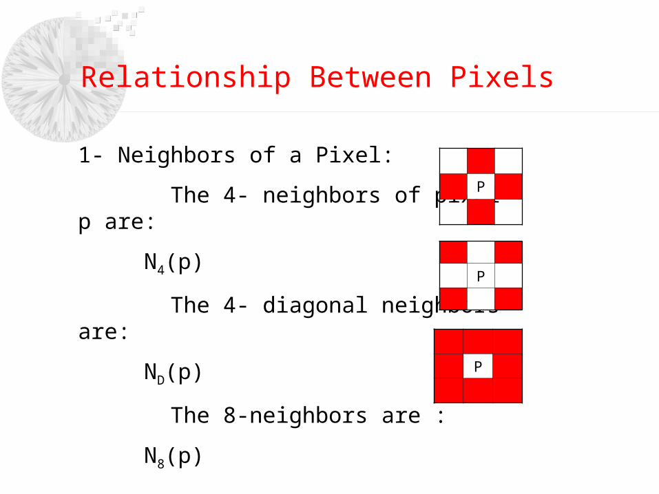
Relationship Between Pixels
Adjacency of Pixels-
Let V be the set of intensity used to define adjacency eg V=1 if we are referring to adjacency of pixels with value 1 in a binary image with 0 and 1In a gray-scale image for the adjacency of pixels with a range of intensity values of say 100 to 120 it follows that V=100101102hellip120We consider three types of adjacency
Adjacency
4- adjacencyTwo pixels p and q with values from V are 4- adjacency if q is in the set N4(p)
Adjacency
8- adjacencyTwo pixels p and q with values from V are 8- adjacency if q is in the set N8(p)
m- adjacency (mixed adjacency)Two pixels p and q with values from V are m- adjacency if
(i) q is in N4(p) or (ii) q is in ND ( p) and N4( p) cap N4 (q) is empty
A (digital) path(or curve) from pixel p at (xy) to pixel q at (st) is a sequence of distinct pixels with coordinates
(x0y0) (x1y1) hellip (xnyn)
where (x0y0) =(xy) (xnyn)=(st) and pixel (xiyi) and (xi-1yi-1) are adjacent for 1le i le n
n is the length of the path
If (x0y0) =(xnyn) the path is a closed path
The path can be defined 4-8-m-paths depending on adjacency type
Path
Connectivity
Let S be a subset of pixels in an image Two pixels p and q are said to be connected in S if there exists a path between them consisting entirely of pixels in SFor any pixel p in S the set of pixels that are connected to it in S is called a connected component of SIf it only has one connected component then set S is called a connected set
Region
Let R be a subset of pixels in an image We call R a region of the image if R is a connected set Two regions are said to be adjacent if their union forms a connected set
Ri Rj are adjacent in 8-adjacency senseThey are not adjacent in 4-adjacency sense
Suppose that an image contains K disjoint regions Rk k = 12 k none of which touches the image border
Let Ru be the union of all the K regions and let (Ru)c denote its complement
We call the points in Ru the foreground and all the points in (Ru)c the background of the imageThe inner boundary (border or contour) of a region R is the set of points that are adjacent to the points in the complement of R ie set of pixels in the region that have at least one background neighbour
Boundary
The point circle is not member of the border of the 1-valued region if 4-connectivity is usedAs a rule adjacency between points in a region and its background is defined in terms of 8-connectivity
Boundary
Boundary
The outer border corresponds to the border in the background This definition to guarantee the existence of a closed path
bull for pixel p q and z with coordinates
(xy) (st) and (uv) respectively
bull D is a distance function or metric if1048708 (a) D(pq) ge 0 D(pq) = 0 iff D=q
1048708 (b) D(pq) = D(qp)
1048708 (c) D(pz) le D(pq) + D(qz)
Distance Measures
1- The Euclidean distance between p and q is defined as
Distance Measures
2- The D4 distance (city-block distance) between p and q is defined as
Distance Measures
3- The D8 distance (chessboard distance) between p and q is defined as
Distance Measures
4- The Dm distance the shortest m-path between the points
Distance Measures
Array product
See matrix multiplication
2221
1211
aa
aa
2221
1211
bb
bb
22222121
12121111
2221
1211
2221
1211
baba
baba
bb
bb
aa
aa
Array Versus Matrix Operations
Linear versus Nonlinear Operations
Consider general operator H
H is said to be a linear operator if
Assume sum operator
)()( yxgyxfH
)()(
)()()()(
yxgayxga
yxfHayxfHayxfayxfaH
jjii
jjiijjii
)()(
)()(
)()()()(
yxgayxga
yxfayxfa
yxfayxfayxfayxfa
jjii
jjii
jjiijjii
Linear versus Nonlinear Operations
Let a1 = 1 a2 =-1
4-
7)1(374
56max)1(
32
20(1)max
2-
42
36max
74
56)1(
32
20)1(max
74
56 and
32
2021
ff
Arithmetic Operations
Carried out between corresponding pixel pairs
Same size of arrays
Let g(xy) denote a corrupted image formed by the addition of noise η(xy) to a noiseless image f(xy)
g(xy) = f(xy) + η(xy)
where the assumption is that at every pair of coordinates (xy) the noise is uncorrelated and has a zero average
)()()(
)()()(
)()()(
)()()(
yxgyxfyxv
yxgyxfyxp
yxgyxfyxd
yxgyxfyxs
Arithmetic Operations
If the noise satisfies the constrains just stated then an image g(xy) is formed by averaging K different noisy images
As K increases the variability of the pixels at each location decreases
)()(
2)(
2)(
1
1
1
)()(
)(1
)(
yxyxg
yxyxg
K
ii
K
K
yxfyxgE
yxgK
yxg
Arithmetic Operations
Arithmetic Operations
Image subtraction is used in the enhancement of the differences between images g(xy) = f(xy) ndash h(xy)
Arithmetic Operations
Application of image multiplication and division is shading correction
If we can get a modeled image as a product of perfect image f(xy) times a shading function h(xy) ie g(xy) = f(xy)h(xy)
If h(xy) is known we can get the perfect image f(xy)
Arithmetic Operations
Multiplication as masking
To solve the range problem in arithmetic operations we can do the following
Given an image f
fm = f ndash min(f) creates an image with min value 0 then
fs = K[fmmax(fm)] creates a scaled image whose range [0 K]
With 8-bit image setting K = 255
Logic Operations
Logic OperationAND p AND q (p q)
OR p OR q (p + q)
COMPLEMENT NOT q ( q )
Logic Operations
Spatial Operations
Performed directly on pixels
Three categoriesSingle-pixel operations
Neighbourhood operations
Geometric spatial transformation
Single-pixel operationsAlter the values of its individual pixels
s = T(z)
Spatial Operations
Neighbourhood operations
Neighbourhood processing generates a corresponding pixel at the same coordinates in an output image
R and c are the row and col Of the pixels whose coordinates are members of the set Sxy
xyScr
crfmn
yxg)(
)(1
)(
Spatial Operations
Geometric spatial transformationModify the spatial relationship between pixels in an image
Consists of two basic operations
Transformation of coordinates Expressed as (xy) = T(vw)
ex (xy) = T(vw) = (v2w2)
Affine transformation (most commonly used)
Scale rotate translate or sheer a set of coordinate points depending on the matrix T
1
0
0
111
3231
2221
1211
tt
tt
tt
wvTwvyx
Spatial Operations
Spatial Operations
The affine equation is used in two ways
Forward mappingScan pixels of the input image
At each location (vw) compute the spatial location (xy)
Two or more pixels in the input image may be transformed to the same location in the output image
Some output locations may not assign a pixel at all
Inverse mapping (more efficient used in commercial MATLAB)Scan the output pixel locations
At each location (xy) compute the spatial location (vw) = T-1(xy)
Interpolate among the nearest input pixels to determine the intensity of the output pixel value
Spatial Operations
Image Registration
Used to align two or more images of the same scene
Input and output images are available but the specific transformation function is not known
Input (image that we wish to transform)
Reference image is the image against which we want to register the input
One approach is using tie points (control points)
The location of the points are precisely known in input and reference images
Using the bilinear approximation is a simple model and given by
x = c1v+c2w+c3vw+c4
y = c5v+c6w+c7vw+c8
(xy) ndash reference image (vw) ndash input image tie points
Image Registration
Four pairs of the corresponding points -gt 8 equations to find the unknown coefficients
Image Transformation
A 2-D transform denoted T(uv) can be expressed in the general form
r(xyuv) forward transformation kernel
s(xyuv) inverse transformation kernel
1
0
1
0
)()()(M
x
N
y
vuyxryxfvuT
1
0
1
0
)()()(M
u
N
v
vuyxsvuTyxf
Image Transformation
Image Transformation
The forward transformation kernel is said to be separable if
kernel is said to be symmetric if r1(xy) is functionally equal to r2(xy) so that
2-D Fourier transform
)()()( 21 vyruxrvuyxr
)()()( 11 vyruxrvuyxr
1
0
1
0
)(2)()(M
x
N
y
NvyMuxjeyxfvuT
1
0
1
0
)(2)(1
)(M
u
N
v
NvyMuxjevuTMN
yxf
Probabilistic Methods
Treating intensities as random quantities is the simplest way of applying probability to image processing
Let zi i=012hellipL-1 possible intensities
Then the probability P(zk ) of intensity level zk is
So
Is the measure of the spread of the value of z about the mean so it is useful to measure an image contrast
MN
nzp k
k )(
1
0
22
1
0
1
0
)()(
)(
1)(
L
kkk
L
kkk
L
kk
zpmz
zpzmaveragemean
zp
Probabilistic Methods
Standard deviation is 143 316 492 intensity level
The variance is 2043 9978 24249

Adjacency
8- adjacencyTwo pixels p and q with values from V are 8- adjacency if q is in the set N8(p)
m- adjacency (mixed adjacency)Two pixels p and q with values from V are m- adjacency if
(i) q is in N4(p) or (ii) q is in ND ( p) and N4( p) cap N4 (q) is empty
A (digital) path(or curve) from pixel p at (xy) to pixel q at (st) is a sequence of distinct pixels with coordinates
(x0y0) (x1y1) hellip (xnyn)
where (x0y0) =(xy) (xnyn)=(st) and pixel (xiyi) and (xi-1yi-1) are adjacent for 1le i le n
n is the length of the path
If (x0y0) =(xnyn) the path is a closed path
The path can be defined 4-8-m-paths depending on adjacency type
Path
Connectivity
Let S be a subset of pixels in an image Two pixels p and q are said to be connected in S if there exists a path between them consisting entirely of pixels in SFor any pixel p in S the set of pixels that are connected to it in S is called a connected component of SIf it only has one connected component then set S is called a connected set
Region
Let R be a subset of pixels in an image We call R a region of the image if R is a connected set Two regions are said to be adjacent if their union forms a connected set
Ri Rj are adjacent in 8-adjacency senseThey are not adjacent in 4-adjacency sense
Suppose that an image contains K disjoint regions Rk k = 12 k none of which touches the image border
Let Ru be the union of all the K regions and let (Ru)c denote its complement
We call the points in Ru the foreground and all the points in (Ru)c the background of the imageThe inner boundary (border or contour) of a region R is the set of points that are adjacent to the points in the complement of R ie set of pixels in the region that have at least one background neighbour
Boundary
The point circle is not member of the border of the 1-valued region if 4-connectivity is usedAs a rule adjacency between points in a region and its background is defined in terms of 8-connectivity
Boundary
Boundary
The outer border corresponds to the border in the background This definition to guarantee the existence of a closed path
bull for pixel p q and z with coordinates
(xy) (st) and (uv) respectively
bull D is a distance function or metric if1048708 (a) D(pq) ge 0 D(pq) = 0 iff D=q
1048708 (b) D(pq) = D(qp)
1048708 (c) D(pz) le D(pq) + D(qz)
Distance Measures
1- The Euclidean distance between p and q is defined as
Distance Measures
2- The D4 distance (city-block distance) between p and q is defined as
Distance Measures
3- The D8 distance (chessboard distance) between p and q is defined as
Distance Measures
4- The Dm distance the shortest m-path between the points
Distance Measures
Array product
See matrix multiplication
2221
1211
aa
aa
2221
1211
bb
bb
22222121
12121111
2221
1211
2221
1211
baba
baba
bb
bb
aa
aa
Array Versus Matrix Operations
Linear versus Nonlinear Operations
Consider general operator H
H is said to be a linear operator if
Assume sum operator
)()( yxgyxfH
)()(
)()()()(
yxgayxga
yxfHayxfHayxfayxfaH
jjii
jjiijjii
)()(
)()(
)()()()(
yxgayxga
yxfayxfa
yxfayxfayxfayxfa
jjii
jjii
jjiijjii
Linear versus Nonlinear Operations
Let a1 = 1 a2 =-1
4-
7)1(374
56max)1(
32
20(1)max
2-
42
36max
74
56)1(
32
20)1(max
74
56 and
32
2021
ff
Arithmetic Operations
Carried out between corresponding pixel pairs
Same size of arrays
Let g(xy) denote a corrupted image formed by the addition of noise η(xy) to a noiseless image f(xy)
g(xy) = f(xy) + η(xy)
where the assumption is that at every pair of coordinates (xy) the noise is uncorrelated and has a zero average
)()()(
)()()(
)()()(
)()()(
yxgyxfyxv
yxgyxfyxp
yxgyxfyxd
yxgyxfyxs
Arithmetic Operations
If the noise satisfies the constrains just stated then an image g(xy) is formed by averaging K different noisy images
As K increases the variability of the pixels at each location decreases
)()(
2)(
2)(
1
1
1
)()(
)(1
)(
yxyxg
yxyxg
K
ii
K
K
yxfyxgE
yxgK
yxg
Arithmetic Operations
Arithmetic Operations
Image subtraction is used in the enhancement of the differences between images g(xy) = f(xy) ndash h(xy)
Arithmetic Operations
Application of image multiplication and division is shading correction
If we can get a modeled image as a product of perfect image f(xy) times a shading function h(xy) ie g(xy) = f(xy)h(xy)
If h(xy) is known we can get the perfect image f(xy)
Arithmetic Operations
Multiplication as masking
To solve the range problem in arithmetic operations we can do the following
Given an image f
fm = f ndash min(f) creates an image with min value 0 then
fs = K[fmmax(fm)] creates a scaled image whose range [0 K]
With 8-bit image setting K = 255
Logic Operations
Logic OperationAND p AND q (p q)
OR p OR q (p + q)
COMPLEMENT NOT q ( q )
Logic Operations
Spatial Operations
Performed directly on pixels
Three categoriesSingle-pixel operations
Neighbourhood operations
Geometric spatial transformation
Single-pixel operationsAlter the values of its individual pixels
s = T(z)
Spatial Operations
Neighbourhood operations
Neighbourhood processing generates a corresponding pixel at the same coordinates in an output image
R and c are the row and col Of the pixels whose coordinates are members of the set Sxy
xyScr
crfmn
yxg)(
)(1
)(
Spatial Operations
Geometric spatial transformationModify the spatial relationship between pixels in an image
Consists of two basic operations
Transformation of coordinates Expressed as (xy) = T(vw)
ex (xy) = T(vw) = (v2w2)
Affine transformation (most commonly used)
Scale rotate translate or sheer a set of coordinate points depending on the matrix T
1
0
0
111
3231
2221
1211
tt
tt
tt
wvTwvyx
Spatial Operations
Spatial Operations
The affine equation is used in two ways
Forward mappingScan pixels of the input image
At each location (vw) compute the spatial location (xy)
Two or more pixels in the input image may be transformed to the same location in the output image
Some output locations may not assign a pixel at all
Inverse mapping (more efficient used in commercial MATLAB)Scan the output pixel locations
At each location (xy) compute the spatial location (vw) = T-1(xy)
Interpolate among the nearest input pixels to determine the intensity of the output pixel value
Spatial Operations
Image Registration
Used to align two or more images of the same scene
Input and output images are available but the specific transformation function is not known
Input (image that we wish to transform)
Reference image is the image against which we want to register the input
One approach is using tie points (control points)
The location of the points are precisely known in input and reference images
Using the bilinear approximation is a simple model and given by
x = c1v+c2w+c3vw+c4
y = c5v+c6w+c7vw+c8
(xy) ndash reference image (vw) ndash input image tie points
Image Registration
Four pairs of the corresponding points -gt 8 equations to find the unknown coefficients
Image Transformation
A 2-D transform denoted T(uv) can be expressed in the general form
r(xyuv) forward transformation kernel
s(xyuv) inverse transformation kernel
1
0
1
0
)()()(M
x
N
y
vuyxryxfvuT
1
0
1
0
)()()(M
u
N
v
vuyxsvuTyxf
Image Transformation
Image Transformation
The forward transformation kernel is said to be separable if
kernel is said to be symmetric if r1(xy) is functionally equal to r2(xy) so that
2-D Fourier transform
)()()( 21 vyruxrvuyxr
)()()( 11 vyruxrvuyxr
1
0
1
0
)(2)()(M
x
N
y
NvyMuxjeyxfvuT
1
0
1
0
)(2)(1
)(M
u
N
v
NvyMuxjevuTMN
yxf
Probabilistic Methods
Treating intensities as random quantities is the simplest way of applying probability to image processing
Let zi i=012hellipL-1 possible intensities
Then the probability P(zk ) of intensity level zk is
So
Is the measure of the spread of the value of z about the mean so it is useful to measure an image contrast
MN
nzp k
k )(
1
0
22
1
0
1
0
)()(
)(
1)(
L
kkk
L
kkk
L
kk
zpmz
zpzmaveragemean
zp
Probabilistic Methods
Standard deviation is 143 316 492 intensity level
The variance is 2043 9978 24249
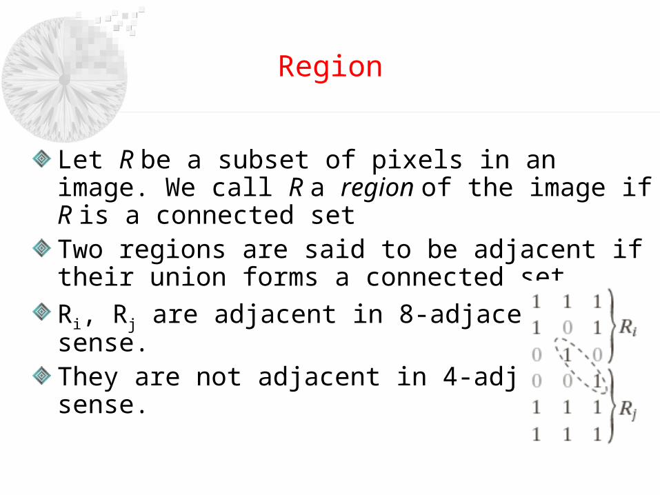
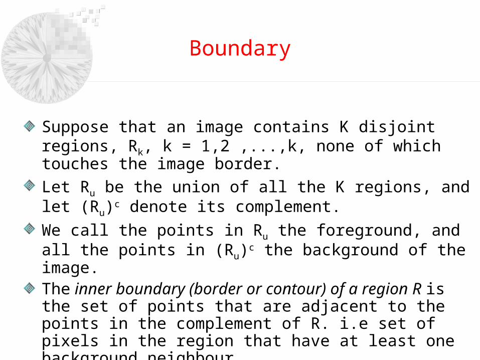
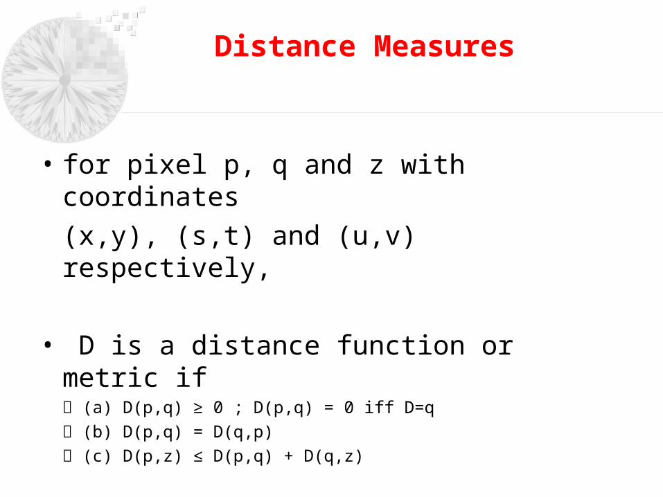
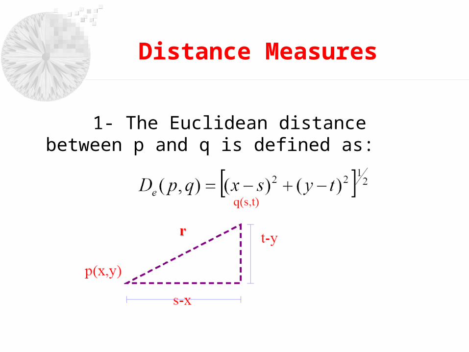
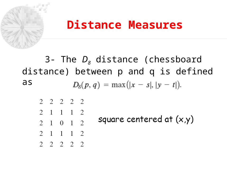
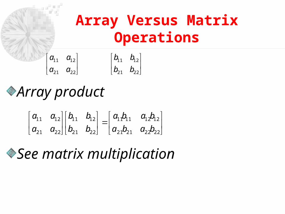

Linear versus Nonlinear Operations
Let a1 = 1 a2 =-1
4-
7)1(374
56max)1(
32
20(1)max
2-
42
36max
74
56)1(
32
20)1(max
74
56 and
32
2021
ff
Arithmetic Operations
Carried out between corresponding pixel pairs
Same size of arrays
Let g(xy) denote a corrupted image formed by the addition of noise η(xy) to a noiseless image f(xy)
g(xy) = f(xy) + η(xy)
where the assumption is that at every pair of coordinates (xy) the noise is uncorrelated and has a zero average
)()()(
)()()(
)()()(
)()()(
yxgyxfyxv
yxgyxfyxp
yxgyxfyxd
yxgyxfyxs
Arithmetic Operations
If the noise satisfies the constrains just stated then an image g(xy) is formed by averaging K different noisy images
As K increases the variability of the pixels at each location decreases
)()(
2)(
2)(
1
1
1
)()(
)(1
)(
yxyxg
yxyxg
K
ii
K
K
yxfyxgE
yxgK
yxg
Arithmetic Operations
Arithmetic Operations
Image subtraction is used in the enhancement of the differences between images g(xy) = f(xy) ndash h(xy)
Arithmetic Operations
Application of image multiplication and division is shading correction
If we can get a modeled image as a product of perfect image f(xy) times a shading function h(xy) ie g(xy) = f(xy)h(xy)
If h(xy) is known we can get the perfect image f(xy)
Arithmetic Operations
Multiplication as masking
To solve the range problem in arithmetic operations we can do the following
Given an image f
fm = f ndash min(f) creates an image with min value 0 then
fs = K[fmmax(fm)] creates a scaled image whose range [0 K]
With 8-bit image setting K = 255
Logic Operations
Logic OperationAND p AND q (p q)
OR p OR q (p + q)
COMPLEMENT NOT q ( q )
Logic Operations
Spatial Operations
Performed directly on pixels
Three categoriesSingle-pixel operations
Neighbourhood operations
Geometric spatial transformation
Single-pixel operationsAlter the values of its individual pixels
s = T(z)
Spatial Operations
Neighbourhood operations
Neighbourhood processing generates a corresponding pixel at the same coordinates in an output image
R and c are the row and col Of the pixels whose coordinates are members of the set Sxy
xyScr
crfmn
yxg)(
)(1
)(
Spatial Operations
Geometric spatial transformationModify the spatial relationship between pixels in an image
Consists of two basic operations
Transformation of coordinates Expressed as (xy) = T(vw)
ex (xy) = T(vw) = (v2w2)
Affine transformation (most commonly used)
Scale rotate translate or sheer a set of coordinate points depending on the matrix T
1
0
0
111
3231
2221
1211
tt
tt
tt
wvTwvyx
Spatial Operations
Spatial Operations
The affine equation is used in two ways
Forward mappingScan pixels of the input image
At each location (vw) compute the spatial location (xy)
Two or more pixels in the input image may be transformed to the same location in the output image
Some output locations may not assign a pixel at all
Inverse mapping (more efficient used in commercial MATLAB)Scan the output pixel locations
At each location (xy) compute the spatial location (vw) = T-1(xy)
Interpolate among the nearest input pixels to determine the intensity of the output pixel value
Spatial Operations
Image Registration
Used to align two or more images of the same scene
Input and output images are available but the specific transformation function is not known
Input (image that we wish to transform)
Reference image is the image against which we want to register the input
One approach is using tie points (control points)
The location of the points are precisely known in input and reference images
Using the bilinear approximation is a simple model and given by
x = c1v+c2w+c3vw+c4
y = c5v+c6w+c7vw+c8
(xy) ndash reference image (vw) ndash input image tie points
Image Registration
Four pairs of the corresponding points -gt 8 equations to find the unknown coefficients
Image Transformation
A 2-D transform denoted T(uv) can be expressed in the general form
r(xyuv) forward transformation kernel
s(xyuv) inverse transformation kernel
1
0
1
0
)()()(M
x
N
y
vuyxryxfvuT
1
0
1
0
)()()(M
u
N
v
vuyxsvuTyxf
Image Transformation
Image Transformation
The forward transformation kernel is said to be separable if
kernel is said to be symmetric if r1(xy) is functionally equal to r2(xy) so that
2-D Fourier transform
)()()( 21 vyruxrvuyxr
)()()( 11 vyruxrvuyxr
1
0
1
0
)(2)()(M
x
N
y
NvyMuxjeyxfvuT
1
0
1
0
)(2)(1
)(M
u
N
v
NvyMuxjevuTMN
yxf
Probabilistic Methods
Treating intensities as random quantities is the simplest way of applying probability to image processing
Let zi i=012hellipL-1 possible intensities
Then the probability P(zk ) of intensity level zk is
So
Is the measure of the spread of the value of z about the mean so it is useful to measure an image contrast
MN
nzp k
k )(
1
0
22
1
0
1
0
)()(
)(
1)(
L
kkk
L
kkk
L
kk
zpmz
zpzmaveragemean
zp
Probabilistic Methods
Standard deviation is 143 316 492 intensity level
The variance is 2043 9978 24249

Arithmetic Operations
Arithmetic Operations
Image subtraction is used in the enhancement of the differences between images g(xy) = f(xy) ndash h(xy)
Arithmetic Operations
Application of image multiplication and division is shading correction
If we can get a modeled image as a product of perfect image f(xy) times a shading function h(xy) ie g(xy) = f(xy)h(xy)
If h(xy) is known we can get the perfect image f(xy)
Arithmetic Operations
Multiplication as masking
To solve the range problem in arithmetic operations we can do the following
Given an image f
fm = f ndash min(f) creates an image with min value 0 then
fs = K[fmmax(fm)] creates a scaled image whose range [0 K]
With 8-bit image setting K = 255
Logic Operations
Logic OperationAND p AND q (p q)
OR p OR q (p + q)
COMPLEMENT NOT q ( q )
Logic Operations
Spatial Operations
Performed directly on pixels
Three categoriesSingle-pixel operations
Neighbourhood operations
Geometric spatial transformation
Single-pixel operationsAlter the values of its individual pixels
s = T(z)
Spatial Operations
Neighbourhood operations
Neighbourhood processing generates a corresponding pixel at the same coordinates in an output image
R and c are the row and col Of the pixels whose coordinates are members of the set Sxy
xyScr
crfmn
yxg)(
)(1
)(
Spatial Operations
Geometric spatial transformationModify the spatial relationship between pixels in an image
Consists of two basic operations
Transformation of coordinates Expressed as (xy) = T(vw)
ex (xy) = T(vw) = (v2w2)
Affine transformation (most commonly used)
Scale rotate translate or sheer a set of coordinate points depending on the matrix T
1
0
0
111
3231
2221
1211
tt
tt
tt
wvTwvyx
Spatial Operations
Spatial Operations
The affine equation is used in two ways
Forward mappingScan pixels of the input image
At each location (vw) compute the spatial location (xy)
Two or more pixels in the input image may be transformed to the same location in the output image
Some output locations may not assign a pixel at all
Inverse mapping (more efficient used in commercial MATLAB)Scan the output pixel locations
At each location (xy) compute the spatial location (vw) = T-1(xy)
Interpolate among the nearest input pixels to determine the intensity of the output pixel value
Spatial Operations
Image Registration
Used to align two or more images of the same scene
Input and output images are available but the specific transformation function is not known
Input (image that we wish to transform)
Reference image is the image against which we want to register the input
One approach is using tie points (control points)
The location of the points are precisely known in input and reference images
Using the bilinear approximation is a simple model and given by
x = c1v+c2w+c3vw+c4
y = c5v+c6w+c7vw+c8
(xy) ndash reference image (vw) ndash input image tie points
Image Registration
Four pairs of the corresponding points -gt 8 equations to find the unknown coefficients
Image Transformation
A 2-D transform denoted T(uv) can be expressed in the general form
r(xyuv) forward transformation kernel
s(xyuv) inverse transformation kernel
1
0
1
0
)()()(M
x
N
y
vuyxryxfvuT
1
0
1
0
)()()(M
u
N
v
vuyxsvuTyxf
Image Transformation
Image Transformation
The forward transformation kernel is said to be separable if
kernel is said to be symmetric if r1(xy) is functionally equal to r2(xy) so that
2-D Fourier transform
)()()( 21 vyruxrvuyxr
)()()( 11 vyruxrvuyxr
1
0
1
0
)(2)()(M
x
N
y
NvyMuxjeyxfvuT
1
0
1
0
)(2)(1
)(M
u
N
v
NvyMuxjevuTMN
yxf
Probabilistic Methods
Treating intensities as random quantities is the simplest way of applying probability to image processing
Let zi i=012hellipL-1 possible intensities
Then the probability P(zk ) of intensity level zk is
So
Is the measure of the spread of the value of z about the mean so it is useful to measure an image contrast
MN
nzp k
k )(
1
0
22
1
0
1
0
)()(
)(
1)(
L
kkk
L
kkk
L
kk
zpmz
zpzmaveragemean
zp
Probabilistic Methods
Standard deviation is 143 316 492 intensity level
The variance is 2043 9978 24249
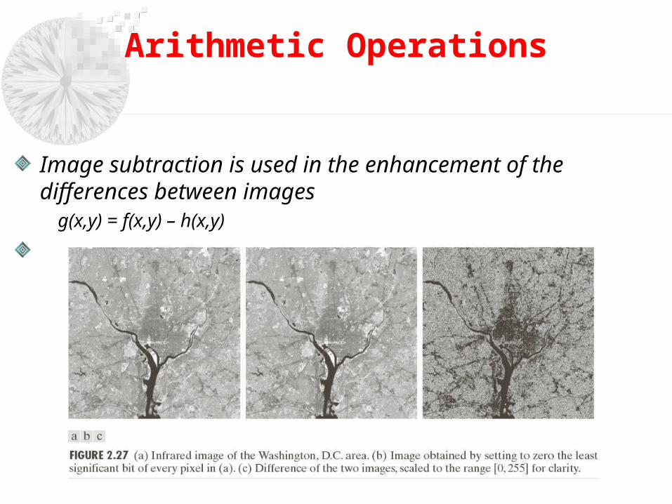
Arithmetic Operations
Image subtraction is used in the enhancement of the differences between images g(xy) = f(xy) ndash h(xy)
Arithmetic Operations
Application of image multiplication and division is shading correction
If we can get a modeled image as a product of perfect image f(xy) times a shading function h(xy) ie g(xy) = f(xy)h(xy)
If h(xy) is known we can get the perfect image f(xy)
Arithmetic Operations
Multiplication as masking
To solve the range problem in arithmetic operations we can do the following
Given an image f
fm = f ndash min(f) creates an image with min value 0 then
fs = K[fmmax(fm)] creates a scaled image whose range [0 K]
With 8-bit image setting K = 255
Logic Operations
Logic OperationAND p AND q (p q)
OR p OR q (p + q)
COMPLEMENT NOT q ( q )
Logic Operations
Spatial Operations
Performed directly on pixels
Three categoriesSingle-pixel operations
Neighbourhood operations
Geometric spatial transformation
Single-pixel operationsAlter the values of its individual pixels
s = T(z)
Spatial Operations
Neighbourhood operations
Neighbourhood processing generates a corresponding pixel at the same coordinates in an output image
R and c are the row and col Of the pixels whose coordinates are members of the set Sxy
xyScr
crfmn
yxg)(
)(1
)(
Spatial Operations
Geometric spatial transformationModify the spatial relationship between pixels in an image
Consists of two basic operations
Transformation of coordinates Expressed as (xy) = T(vw)
ex (xy) = T(vw) = (v2w2)
Affine transformation (most commonly used)
Scale rotate translate or sheer a set of coordinate points depending on the matrix T
1
0
0
111
3231
2221
1211
tt
tt
tt
wvTwvyx
Spatial Operations
Spatial Operations
The affine equation is used in two ways
Forward mappingScan pixels of the input image
At each location (vw) compute the spatial location (xy)
Two or more pixels in the input image may be transformed to the same location in the output image
Some output locations may not assign a pixel at all
Inverse mapping (more efficient used in commercial MATLAB)Scan the output pixel locations
At each location (xy) compute the spatial location (vw) = T-1(xy)
Interpolate among the nearest input pixels to determine the intensity of the output pixel value
Spatial Operations
Image Registration
Used to align two or more images of the same scene
Input and output images are available but the specific transformation function is not known
Input (image that we wish to transform)
Reference image is the image against which we want to register the input
One approach is using tie points (control points)
The location of the points are precisely known in input and reference images
Using the bilinear approximation is a simple model and given by
x = c1v+c2w+c3vw+c4
y = c5v+c6w+c7vw+c8
(xy) ndash reference image (vw) ndash input image tie points
Image Registration
Four pairs of the corresponding points -gt 8 equations to find the unknown coefficients
Image Transformation
A 2-D transform denoted T(uv) can be expressed in the general form
r(xyuv) forward transformation kernel
s(xyuv) inverse transformation kernel
1
0
1
0
)()()(M
x
N
y
vuyxryxfvuT
1
0
1
0
)()()(M
u
N
v
vuyxsvuTyxf
Image Transformation
Image Transformation
The forward transformation kernel is said to be separable if
kernel is said to be symmetric if r1(xy) is functionally equal to r2(xy) so that
2-D Fourier transform
)()()( 21 vyruxrvuyxr
)()()( 11 vyruxrvuyxr
1
0
1
0
)(2)()(M
x
N
y
NvyMuxjeyxfvuT
1
0
1
0
)(2)(1
)(M
u
N
v
NvyMuxjevuTMN
yxf
Probabilistic Methods
Treating intensities as random quantities is the simplest way of applying probability to image processing
Let zi i=012hellipL-1 possible intensities
Then the probability P(zk ) of intensity level zk is
So
Is the measure of the spread of the value of z about the mean so it is useful to measure an image contrast
MN
nzp k
k )(
1
0
22
1
0
1
0
)()(
)(
1)(
L
kkk
L
kkk
L
kk
zpmz
zpzmaveragemean
zp
Probabilistic Methods
Standard deviation is 143 316 492 intensity level
The variance is 2043 9978 24249
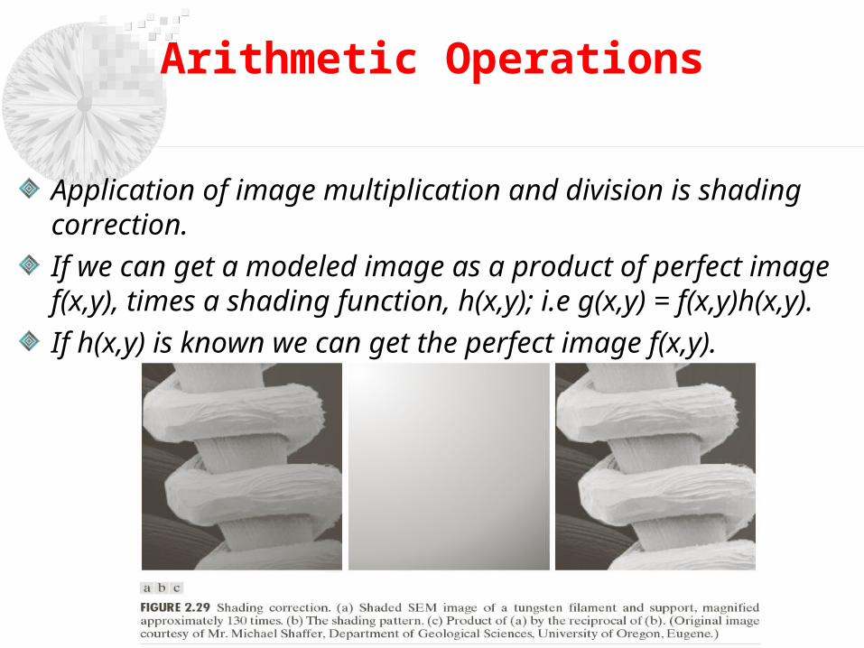
Arithmetic Operations
Multiplication as masking
To solve the range problem in arithmetic operations we can do the following
Given an image f
fm = f ndash min(f) creates an image with min value 0 then
fs = K[fmmax(fm)] creates a scaled image whose range [0 K]
With 8-bit image setting K = 255
Logic Operations
Logic OperationAND p AND q (p q)
OR p OR q (p + q)
COMPLEMENT NOT q ( q )
Logic Operations
Spatial Operations
Performed directly on pixels
Three categoriesSingle-pixel operations
Neighbourhood operations
Geometric spatial transformation
Single-pixel operationsAlter the values of its individual pixels
s = T(z)
Spatial Operations
Neighbourhood operations
Neighbourhood processing generates a corresponding pixel at the same coordinates in an output image
R and c are the row and col Of the pixels whose coordinates are members of the set Sxy
xyScr
crfmn
yxg)(
)(1
)(
Spatial Operations
Geometric spatial transformationModify the spatial relationship between pixels in an image
Consists of two basic operations
Transformation of coordinates Expressed as (xy) = T(vw)
ex (xy) = T(vw) = (v2w2)
Affine transformation (most commonly used)
Scale rotate translate or sheer a set of coordinate points depending on the matrix T
1
0
0
111
3231
2221
1211
tt
tt
tt
wvTwvyx
Spatial Operations
Spatial Operations
The affine equation is used in two ways
Forward mappingScan pixels of the input image
At each location (vw) compute the spatial location (xy)
Two or more pixels in the input image may be transformed to the same location in the output image
Some output locations may not assign a pixel at all
Inverse mapping (more efficient used in commercial MATLAB)Scan the output pixel locations
At each location (xy) compute the spatial location (vw) = T-1(xy)
Interpolate among the nearest input pixels to determine the intensity of the output pixel value
Spatial Operations
Image Registration
Used to align two or more images of the same scene
Input and output images are available but the specific transformation function is not known
Input (image that we wish to transform)
Reference image is the image against which we want to register the input
One approach is using tie points (control points)
The location of the points are precisely known in input and reference images
Using the bilinear approximation is a simple model and given by
x = c1v+c2w+c3vw+c4
y = c5v+c6w+c7vw+c8
(xy) ndash reference image (vw) ndash input image tie points
Image Registration
Four pairs of the corresponding points -gt 8 equations to find the unknown coefficients
Image Transformation
A 2-D transform denoted T(uv) can be expressed in the general form
r(xyuv) forward transformation kernel
s(xyuv) inverse transformation kernel
1
0
1
0
)()()(M
x
N
y
vuyxryxfvuT
1
0
1
0
)()()(M
u
N
v
vuyxsvuTyxf
Image Transformation
Image Transformation
The forward transformation kernel is said to be separable if
kernel is said to be symmetric if r1(xy) is functionally equal to r2(xy) so that
2-D Fourier transform
)()()( 21 vyruxrvuyxr
)()()( 11 vyruxrvuyxr
1
0
1
0
)(2)()(M
x
N
y
NvyMuxjeyxfvuT
1
0
1
0
)(2)(1
)(M
u
N
v
NvyMuxjevuTMN
yxf
Probabilistic Methods
Treating intensities as random quantities is the simplest way of applying probability to image processing
Let zi i=012hellipL-1 possible intensities
Then the probability P(zk ) of intensity level zk is
So
Is the measure of the spread of the value of z about the mean so it is useful to measure an image contrast
MN
nzp k
k )(
1
0
22
1
0
1
0
)()(
)(
1)(
L
kkk
L
kkk
L
kk
zpmz
zpzmaveragemean
zp
Probabilistic Methods
Standard deviation is 143 316 492 intensity level
The variance is 2043 9978 24249

Logic Operations
Spatial Operations
Performed directly on pixels
Three categoriesSingle-pixel operations
Neighbourhood operations
Geometric spatial transformation
Single-pixel operationsAlter the values of its individual pixels
s = T(z)
Spatial Operations
Neighbourhood operations
Neighbourhood processing generates a corresponding pixel at the same coordinates in an output image
R and c are the row and col Of the pixels whose coordinates are members of the set Sxy
xyScr
crfmn
yxg)(
)(1
)(
Spatial Operations
Geometric spatial transformationModify the spatial relationship between pixels in an image
Consists of two basic operations
Transformation of coordinates Expressed as (xy) = T(vw)
ex (xy) = T(vw) = (v2w2)
Affine transformation (most commonly used)
Scale rotate translate or sheer a set of coordinate points depending on the matrix T
1
0
0
111
3231
2221
1211
tt
tt
tt
wvTwvyx
Spatial Operations
Spatial Operations
The affine equation is used in two ways
Forward mappingScan pixels of the input image
At each location (vw) compute the spatial location (xy)
Two or more pixels in the input image may be transformed to the same location in the output image
Some output locations may not assign a pixel at all
Inverse mapping (more efficient used in commercial MATLAB)Scan the output pixel locations
At each location (xy) compute the spatial location (vw) = T-1(xy)
Interpolate among the nearest input pixels to determine the intensity of the output pixel value
Spatial Operations
Image Registration
Used to align two or more images of the same scene
Input and output images are available but the specific transformation function is not known
Input (image that we wish to transform)
Reference image is the image against which we want to register the input
One approach is using tie points (control points)
The location of the points are precisely known in input and reference images
Using the bilinear approximation is a simple model and given by
x = c1v+c2w+c3vw+c4
y = c5v+c6w+c7vw+c8
(xy) ndash reference image (vw) ndash input image tie points
Image Registration
Four pairs of the corresponding points -gt 8 equations to find the unknown coefficients
Image Transformation
A 2-D transform denoted T(uv) can be expressed in the general form
r(xyuv) forward transformation kernel
s(xyuv) inverse transformation kernel
1
0
1
0
)()()(M
x
N
y
vuyxryxfvuT
1
0
1
0
)()()(M
u
N
v
vuyxsvuTyxf
Image Transformation
Image Transformation
The forward transformation kernel is said to be separable if
kernel is said to be symmetric if r1(xy) is functionally equal to r2(xy) so that
2-D Fourier transform
)()()( 21 vyruxrvuyxr
)()()( 11 vyruxrvuyxr
1
0
1
0
)(2)()(M
x
N
y
NvyMuxjeyxfvuT
1
0
1
0
)(2)(1
)(M
u
N
v
NvyMuxjevuTMN
yxf
Probabilistic Methods
Treating intensities as random quantities is the simplest way of applying probability to image processing
Let zi i=012hellipL-1 possible intensities
Then the probability P(zk ) of intensity level zk is
So
Is the measure of the spread of the value of z about the mean so it is useful to measure an image contrast
MN
nzp k
k )(
1
0
22
1
0
1
0
)()(
)(
1)(
L
kkk
L
kkk
L
kk
zpmz
zpzmaveragemean
zp
Probabilistic Methods
Standard deviation is 143 316 492 intensity level
The variance is 2043 9978 24249

Spatial Operations
Performed directly on pixels
Three categoriesSingle-pixel operations
Neighbourhood operations
Geometric spatial transformation
Single-pixel operationsAlter the values of its individual pixels
s = T(z)
Spatial Operations
Neighbourhood operations
Neighbourhood processing generates a corresponding pixel at the same coordinates in an output image
R and c are the row and col Of the pixels whose coordinates are members of the set Sxy
xyScr
crfmn
yxg)(
)(1
)(
Spatial Operations
Geometric spatial transformationModify the spatial relationship between pixels in an image
Consists of two basic operations
Transformation of coordinates Expressed as (xy) = T(vw)
ex (xy) = T(vw) = (v2w2)
Affine transformation (most commonly used)
Scale rotate translate or sheer a set of coordinate points depending on the matrix T
1
0
0
111
3231
2221
1211
tt
tt
tt
wvTwvyx
Spatial Operations
Spatial Operations
The affine equation is used in two ways
Forward mappingScan pixels of the input image
At each location (vw) compute the spatial location (xy)
Two or more pixels in the input image may be transformed to the same location in the output image
Some output locations may not assign a pixel at all
Inverse mapping (more efficient used in commercial MATLAB)Scan the output pixel locations
At each location (xy) compute the spatial location (vw) = T-1(xy)
Interpolate among the nearest input pixels to determine the intensity of the output pixel value
Spatial Operations
Image Registration
Used to align two or more images of the same scene
Input and output images are available but the specific transformation function is not known
Input (image that we wish to transform)
Reference image is the image against which we want to register the input
One approach is using tie points (control points)
The location of the points are precisely known in input and reference images
Using the bilinear approximation is a simple model and given by
x = c1v+c2w+c3vw+c4
y = c5v+c6w+c7vw+c8
(xy) ndash reference image (vw) ndash input image tie points
Image Registration
Four pairs of the corresponding points -gt 8 equations to find the unknown coefficients
Image Transformation
A 2-D transform denoted T(uv) can be expressed in the general form
r(xyuv) forward transformation kernel
s(xyuv) inverse transformation kernel
1
0
1
0
)()()(M
x
N
y
vuyxryxfvuT
1
0
1
0
)()()(M
u
N
v
vuyxsvuTyxf
Image Transformation
Image Transformation
The forward transformation kernel is said to be separable if
kernel is said to be symmetric if r1(xy) is functionally equal to r2(xy) so that
2-D Fourier transform
)()()( 21 vyruxrvuyxr
)()()( 11 vyruxrvuyxr
1
0
1
0
)(2)()(M
x
N
y
NvyMuxjeyxfvuT
1
0
1
0
)(2)(1
)(M
u
N
v
NvyMuxjevuTMN
yxf
Probabilistic Methods
Treating intensities as random quantities is the simplest way of applying probability to image processing
Let zi i=012hellipL-1 possible intensities
Then the probability P(zk ) of intensity level zk is
So
Is the measure of the spread of the value of z about the mean so it is useful to measure an image contrast
MN
nzp k
k )(
1
0
22
1
0
1
0
)()(
)(
1)(
L
kkk
L
kkk
L
kk
zpmz
zpzmaveragemean
zp
Probabilistic Methods
Standard deviation is 143 316 492 intensity level
The variance is 2043 9978 24249
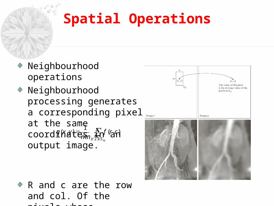
Spatial Operations
Spatial Operations
The affine equation is used in two ways
Forward mappingScan pixels of the input image
At each location (vw) compute the spatial location (xy)
Two or more pixels in the input image may be transformed to the same location in the output image
Some output locations may not assign a pixel at all
Inverse mapping (more efficient used in commercial MATLAB)Scan the output pixel locations
At each location (xy) compute the spatial location (vw) = T-1(xy)
Interpolate among the nearest input pixels to determine the intensity of the output pixel value
Spatial Operations
Image Registration
Used to align two or more images of the same scene
Input and output images are available but the specific transformation function is not known
Input (image that we wish to transform)
Reference image is the image against which we want to register the input
One approach is using tie points (control points)
The location of the points are precisely known in input and reference images
Using the bilinear approximation is a simple model and given by
x = c1v+c2w+c3vw+c4
y = c5v+c6w+c7vw+c8
(xy) ndash reference image (vw) ndash input image tie points
Image Registration
Four pairs of the corresponding points -gt 8 equations to find the unknown coefficients
Image Transformation
A 2-D transform denoted T(uv) can be expressed in the general form
r(xyuv) forward transformation kernel
s(xyuv) inverse transformation kernel
1
0
1
0
)()()(M
x
N
y
vuyxryxfvuT
1
0
1
0
)()()(M
u
N
v
vuyxsvuTyxf
Image Transformation
Image Transformation
The forward transformation kernel is said to be separable if
kernel is said to be symmetric if r1(xy) is functionally equal to r2(xy) so that
2-D Fourier transform
)()()( 21 vyruxrvuyxr
)()()( 11 vyruxrvuyxr
1
0
1
0
)(2)()(M
x
N
y
NvyMuxjeyxfvuT
1
0
1
0
)(2)(1
)(M
u
N
v
NvyMuxjevuTMN
yxf
Probabilistic Methods
Treating intensities as random quantities is the simplest way of applying probability to image processing
Let zi i=012hellipL-1 possible intensities
Then the probability P(zk ) of intensity level zk is
So
Is the measure of the spread of the value of z about the mean so it is useful to measure an image contrast
MN
nzp k
k )(
1
0
22
1
0
1
0
)()(
)(
1)(
L
kkk
L
kkk
L
kk
zpmz
zpzmaveragemean
zp
Probabilistic Methods
Standard deviation is 143 316 492 intensity level
The variance is 2043 9978 24249

Spatial Operations
Image Registration
Used to align two or more images of the same scene
Input and output images are available but the specific transformation function is not known
Input (image that we wish to transform)
Reference image is the image against which we want to register the input
One approach is using tie points (control points)
The location of the points are precisely known in input and reference images
Using the bilinear approximation is a simple model and given by
x = c1v+c2w+c3vw+c4
y = c5v+c6w+c7vw+c8
(xy) ndash reference image (vw) ndash input image tie points
Image Registration
Four pairs of the corresponding points -gt 8 equations to find the unknown coefficients
Image Transformation
A 2-D transform denoted T(uv) can be expressed in the general form
r(xyuv) forward transformation kernel
s(xyuv) inverse transformation kernel
1
0
1
0
)()()(M
x
N
y
vuyxryxfvuT
1
0
1
0
)()()(M
u
N
v
vuyxsvuTyxf
Image Transformation
Image Transformation
The forward transformation kernel is said to be separable if
kernel is said to be symmetric if r1(xy) is functionally equal to r2(xy) so that
2-D Fourier transform
)()()( 21 vyruxrvuyxr
)()()( 11 vyruxrvuyxr
1
0
1
0
)(2)()(M
x
N
y
NvyMuxjeyxfvuT
1
0
1
0
)(2)(1
)(M
u
N
v
NvyMuxjevuTMN
yxf
Probabilistic Methods
Treating intensities as random quantities is the simplest way of applying probability to image processing
Let zi i=012hellipL-1 possible intensities
Then the probability P(zk ) of intensity level zk is
So
Is the measure of the spread of the value of z about the mean so it is useful to measure an image contrast
MN
nzp k
k )(
1
0
22
1
0
1
0
)()(
)(
1)(
L
kkk
L
kkk
L
kk
zpmz
zpzmaveragemean
zp
Probabilistic Methods
Standard deviation is 143 316 492 intensity level
The variance is 2043 9978 24249

Image Registration
Four pairs of the corresponding points -gt 8 equations to find the unknown coefficients
Image Transformation
A 2-D transform denoted T(uv) can be expressed in the general form
r(xyuv) forward transformation kernel
s(xyuv) inverse transformation kernel
1
0
1
0
)()()(M
x
N
y
vuyxryxfvuT
1
0
1
0
)()()(M
u
N
v
vuyxsvuTyxf
Image Transformation
Image Transformation
The forward transformation kernel is said to be separable if
kernel is said to be symmetric if r1(xy) is functionally equal to r2(xy) so that
2-D Fourier transform
)()()( 21 vyruxrvuyxr
)()()( 11 vyruxrvuyxr
1
0
1
0
)(2)()(M
x
N
y
NvyMuxjeyxfvuT
1
0
1
0
)(2)(1
)(M
u
N
v
NvyMuxjevuTMN
yxf
Probabilistic Methods
Treating intensities as random quantities is the simplest way of applying probability to image processing
Let zi i=012hellipL-1 possible intensities
Then the probability P(zk ) of intensity level zk is
So
Is the measure of the spread of the value of z about the mean so it is useful to measure an image contrast
MN
nzp k
k )(
1
0
22
1
0
1
0
)()(
)(
1)(
L
kkk
L
kkk
L
kk
zpmz
zpzmaveragemean
zp
Probabilistic Methods
Standard deviation is 143 316 492 intensity level
The variance is 2043 9978 24249

Image Transformation
Image Transformation
The forward transformation kernel is said to be separable if
kernel is said to be symmetric if r1(xy) is functionally equal to r2(xy) so that
2-D Fourier transform
)()()( 21 vyruxrvuyxr
)()()( 11 vyruxrvuyxr
1
0
1
0
)(2)()(M
x
N
y
NvyMuxjeyxfvuT
1
0
1
0
)(2)(1
)(M
u
N
v
NvyMuxjevuTMN
yxf
Probabilistic Methods
Treating intensities as random quantities is the simplest way of applying probability to image processing
Let zi i=012hellipL-1 possible intensities
Then the probability P(zk ) of intensity level zk is
So
Is the measure of the spread of the value of z about the mean so it is useful to measure an image contrast
MN
nzp k
k )(
1
0
22
1
0
1
0
)()(
)(
1)(
L
kkk
L
kkk
L
kk
zpmz
zpzmaveragemean
zp
Probabilistic Methods
Standard deviation is 143 316 492 intensity level
The variance is 2043 9978 24249
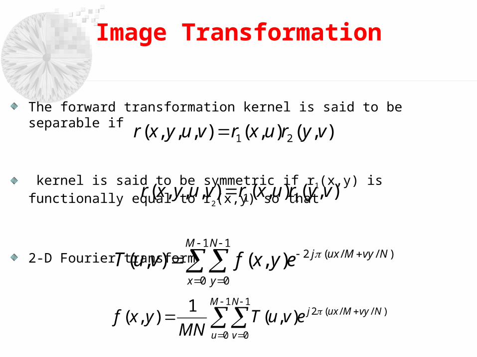
Image Transformation
The forward transformation kernel is said to be separable if
kernel is said to be symmetric if r1(xy) is functionally equal to r2(xy) so that
2-D Fourier transform
)()()( 21 vyruxrvuyxr
)()()( 11 vyruxrvuyxr
1
0
1
0
)(2)()(M
x
N
y
NvyMuxjeyxfvuT
1
0
1
0
)(2)(1
)(M
u
N
v
NvyMuxjevuTMN
yxf
Probabilistic Methods
Treating intensities as random quantities is the simplest way of applying probability to image processing
Let zi i=012hellipL-1 possible intensities
Then the probability P(zk ) of intensity level zk is
So
Is the measure of the spread of the value of z about the mean so it is useful to measure an image contrast
MN
nzp k
k )(
1
0
22
1
0
1
0
)()(
)(
1)(
L
kkk
L
kkk
L
kk
zpmz
zpzmaveragemean
zp
Probabilistic Methods
Standard deviation is 143 316 492 intensity level
The variance is 2043 9978 24249

Probabilistic Methods
Standard deviation is 143 316 492 intensity level
The variance is 2043 9978 24249