Chapter Three Applying the Supply- and-Demand Model

Chapter Three

Applying the Supply-and-Demand Model

© 2009 Pearson Addison-Wesley. All rights reserved. 3-2

Topics To Be Covered

How the shapes of demand and supply curves matter?

Sensitivity of quantity demanded to price.

Sensitivity of quantity supplied to price. Long run versus short run Effects of a sales tax.


How shapes of demand and supply matter?

The shapes of the demand and supply curves determine by how much a shock affects the equilibrium price and quantity.

Example: processed pork (same as Chapter 2) Supply depends on the price of pork and

the price of hogs.

© 2007 Pearson Addison-Wesley. All rights reserved. 3–4

Figure 3.1 How the Effect of a Supply Shock Depends on the Shape of the Demand Curve

(a) (b) (c)

215 2201760Q, Million kg of pork per year

3.553.30

S 1

D1

S 2 e1

e2

2201760Q, Million kg of pork per year

3.6753.30

S 1S 2

D2

e1

e2

2202051760Q, Million kg of pork per year

3.30

S 1S 2

D3e

1

e2


Figure 3.1 How the Effect of a Supply Shock Depends on the Shape of the Demand Curve (cont’d)

3.30

220

Q, Million kg of pork per year

p,

$ p

er k

g

2051760

(c)

e1

e2D3

S1S2

When demand is very sensitive to price… a shift in the supply

curve to S2… has no effect on the

equilibrium price and a substantial effect

on the quantity


Sensitivity of quantity demanded to price.

Elasticity – the percentage change in a variable in response to a given percentage change in another variable, all other factors held constant.


Elasticity

price in %

demandedquantity in %

demand of elasticity Price

et variablindependen in%

variabledependent in %

Price elasticity of demand

() – the percentage change in the quantity demanded in response to a given percentage change in the price.

Elastic demand <-1 or |E| >1

Unit elastic demand E=-1 or |E| =1

Inelastic demand 0>E>-1 or 0<|E|<1


Price Elasticity and Total Revenue

Total revenue = price x quantity Elastic demand

Price and total revenue inversely related

Inelastic demand Price and total revenue are directly related

Unit elastic demand No change in total revenue in response to a

change in price



Sensitivity of quantity demanded to price (cont).

Formally,

where indicates change.

Example If a 1% increase in price results in a 3% decrease in

quantity demanded, the elasticity of demand is = -3%/1% = -3.

Q

p

p

Q

pp

QQ

p

Q

%

%


Sensitivity of quantity demanded to price (cont).

Along linear demand curve with a function of:

Where -b is the slope or

the elasticity of demand is

bpaQ

p

Qb

(3.3) /

/

Q

pb

Q

p

p

Q

pp

QQ


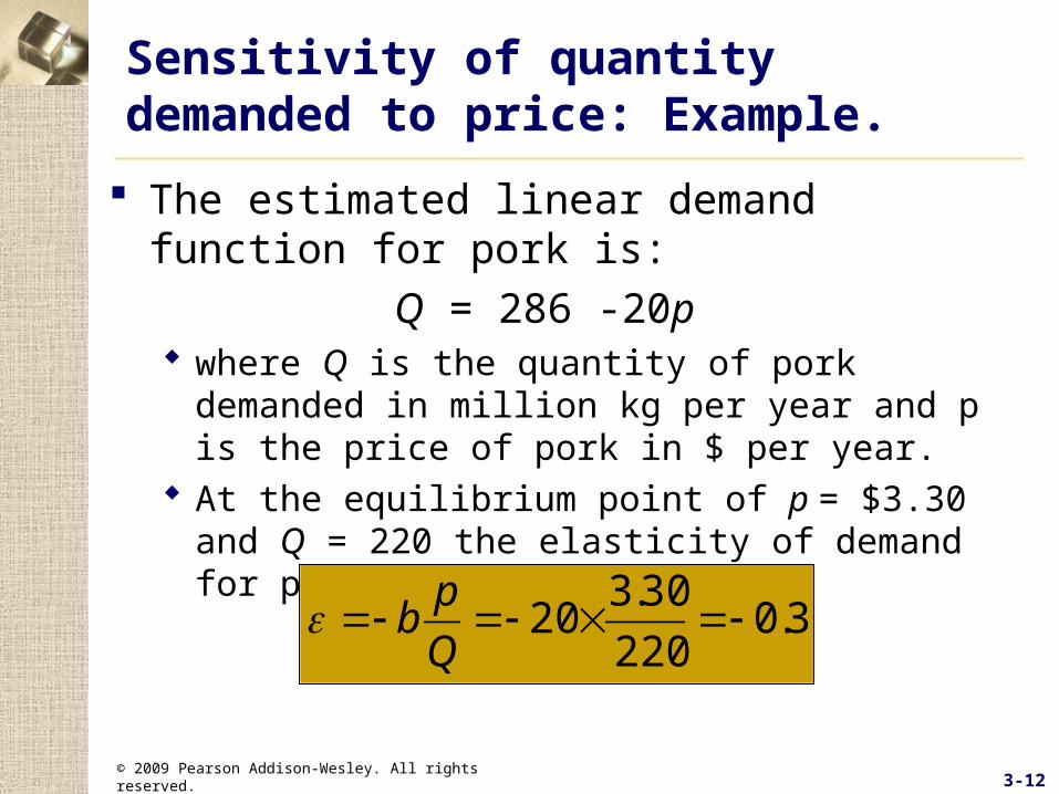
Sensitivity of quantity demanded to price: Example.

The estimated linear demand function for pork is:

Q = 286 -20p where Q is the quantity of pork demanded in million

kg per year and p is the price of pork in $ per year. At the equilibrium point of p = $3.30 and Q = 220

the elasticity of demand for pork is

3.0220

30.320

Q

pb


Elasticity: An Application and a practice problem

Varian (2002) found that the price elasticity of demand for internet use was -2.0 for those who used a 128 Kbps service -2.9 for those who used a 64 Kbps service.

Practice problem: A 1% increase in the price per minute reduced the

connection time by ________ for those with high speed access, and by _______ for those with slow phone line access.


Elasticity Along a Demand Curve

The elasticity of demand varies along most demand curves. Along a downward-sloping linear demand curve the

elasticity of demand is a more negative number the higher the price is.


Figure 3.2 Elasticity Along the Pork Demand Curve

p, $

pe

r kg

a/2 = 143a/5 = 57.2

D

a = 286220


0

11.44

a/b = 14.30

3.30

a/(2b) = 7.15

Elastic < –1 = –4

= –0.3

Inelastic 0 > > –1

Perfectlyinelastic

Perfectly elastic

Unitary: = -1

Q = 286 -20p

= -bp

Q = -20 x 11.4457.2 = -4

3.30220 = -0.3


Elasticity Along The Demand Curve: Practice Problem

According to Agcaoli-Sombilla (1991), the elasticity of demand for rice is -0.47 in Austria; -0.8 in Bangladesh, China, India, Indonesia, and Thailand; -0.25 in Japan; -0.55 in the EU and the US; and -0.15 in Vietnam. In which countries is the demand for rice

inelastic? In all the countries, since in all cases > -1.

In which country is the least elastic? In Vietnam, where = -0.15


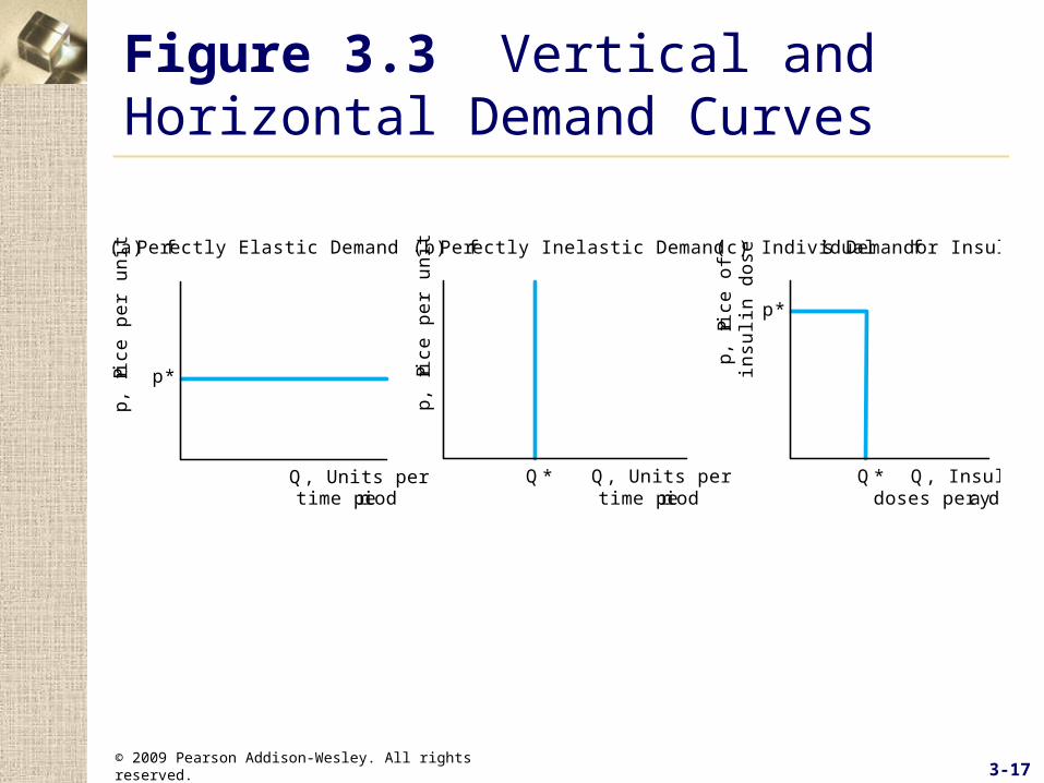
Figure 3.3 Vertical and Horizontal Demand Curves

p, P

rice

pe

r u

nit

(a) Perfectly Elastic Demand

Q, Units pertime period

p*

(b) Perfectly Inelastic Demand

p, P

rice

pe

r u

nit

Q* Q, Units pertime period

(c) Individual’s Demand for Insulin

p*

p, P

rice

of

insu

lin d

ose

Q* Q, Insulindoses per day

Price Elasticity of Demand


The absolute percentage change in the quantity demanded is smaller than the absolute percentage change in price so that the price elasticity of demand is less than 1 and the good has inelastic demand.

If the percentage change in the quantity demanded is infinitely large when the price barely changes, the price elasticity of demand is infinite and the good has perfectly elastic demand.



If the absolute percentage change in the quantity demanded is greater than the absolute percentage change in price, the price elasticity of demand is greater than 1 and the good has elastic demand.



The Factors That Influence the Elasticity of DemandThe elasticity of demand for a good depends on: The closeness of substitutes The proportion of income spent on the good The definition of the market The time elapsed since a price change


Price Elasticity

Q

pb

bpaQ

Q

p

p

Q

pp

QQ

./

/

Constant elasticity demand function


P

PPQPPQ

PPQ

PQ

PQ

1

1

)()/)(/(.3

)(/.2

logloglog

.1


Sensitivity of quantity demanded to income. Formally,

where Y stands for income.

Example If a 1% increase in income results in a 3% decrease in

quantity demanded, the income elasticity of demand is = -3%/1% = -3.

Q

Y

Y

Q

YY

QQ

Y

Q

%

%


Sensitivity of quantity demanded to income: Example.

The estimated demand function for pork is:

Q = 171 – 20p + 20pb + 3pc + 2Y where p is the price of pork ($3.00), pb is the price

of beef ($4.00), pc is the price of chicken ($3.33) and Y is the income (in thousands of dollars) (12.5).

Question: what would be the income elasticity of demand for Pork if Q = 220 and Y = 12.5

Answer: Since = 2, then

114.0220

5.1222

Q

Y

Q

Y

Y

QY

Q


Calculating Elasticities

The estimated demand function for pork is:

Q = 171 – 20p + 20pb + 3pc + 2Y where p is the price of pork ($3.00), pb is the price

of beef ($4.00), pc is the price of chicken ($3.33) and Y is the income (in thousands of dollars) (12.5).

Then Q = 171 – 20(3.30) + 20(4) +3 (3.33) + 2 (12.5) Q=171-66+80+10+25 Q=20

Calculating Price Elasticity of Demand

Q = 171 – 20p + 20pb + 3pc + 2Y

Q=220, p=3.30


3.220

30.320

Q

p

p

QD

Calculating Cross Price Elasticity

Q = 171 – 20p + 20pb + 3pc + 2Y

Q=220, pb=4.00


36.220

00.420

Q

p

p

Q b

bxy


Sensitivity of quantity demanded to the price of a related good. If the cross-price elasticity is positive, the

goods are substitutes. Question: can you think of any examples of two

goods that are substitutes? Roses and carnations.

If the cross-price elasticity is negative, the goods are complements Question: can you think of any examples of two

goods that are complements? Peanut butter and jelly

Calculating Income Elasticity

Q = 171 – 20p + 20pb + 3pc + 2Y

Q=220, Y=12.5


114.220

5.122

Q

Y

Y

QY

Income Elasticity

EY>0, normal good

EY>1, normal and superior

EY<0, inferior good

Identify proportional changes in budget expenditure



Sensitivity of quantity supplied to price. Formally,

where Q indicates quantity supplied. Example

If a 1% increase in price results in a 3% increase in quantity supplied, the elasticity of supplied is = 3%/1% = 3.

Q

p

p

Q

pp

QQ

p

Q

%

%


Sensitivity of quantity demanded to price: Example.

The estimated linear supply function for pork is:

Q = 88 - 40p where Q is the quantity of pork supplied in million

kg per year and p is the price of pork in $ per year. At the equilibrium, where p = $3.30 and Q = 220,

the elasticity of supplied is:

6.0220

30.340

Q

P

p

Q


Sensitivity of quantity supplied to price (cont).

Along linear supply curve with a function of:

Where -b is the slope or

the elasticity of demand is

hpgQ

p

Qh

Q

ph

Q

p

p

Q


Figure 3.4 Elasticity Along the Pork Supply Curve


Demand Elasticities Over Time

Elasticities tend to be larger in the long-run. Can you think why?

In the case of demand:– Substitution and storage opportunities.

In the case of supply:– Converting fixed inputs into variable inputs.


Effects of a Sales Tax

1. What effect does a sales tax have on equilibrium prices and quantity?

2. Is it true, as many people claim, that taxes assessed on producers are passed along to consumers?

3. Do the equilibrium price and quantity depend on whether the tax is assessed on consumers or on producers?


Two Types of Sales Taxes

Ad valorem tax - for every dollar the consumer spends, the government keeps a fraction, α, which is the ad valorem tax rate.

Unit tax - where a specified dollar amount, , is collected per unit of output.


Figure 3.5 Effect of a $1.05 Specific Tax on the Pork Market Collected from Producers

A tax on producers shifts the supply curve downward by the amount of the tax (= $1.05)….

which causes the market price to increase…

After the tax, buyers are worse off by

$0.70 ($4.00 - $3.30)… sellers are worse off by

$0.35 ($3.30 - $2.95) and the government

collects $216.3 in revenue.

p, $

pe

r kg

Q2 = 206 Q1 = 220176

T = $216.3 million


0

p2 = 4.00

p3 = 3.30

p2 – = 2.95

= $1.05 S1

e1

e2

S2

D

Solution to Excise Tax ProblemUnit Tax on Producers


tpdcQ

bpaQ

p-t

dpcQ

bpaQ

s

d

s

d

receiveonly producers t ofa tax With


Figure 3.6 Effect of a $1.05 Specific Tax on Pork Collected from Consumers

p,

$ p

er

kg

Q2 = 206 Q1 = 220176

T = $216.3 million

Q, Million kg of pork per year0

p = 4.00

p = 3.30

p2 – = 2.95

= $1.05

Wedge, = $1.05

D1

D2

e2

e2S

The tax shifts the demand curve down by τ = $1.05…

but the new equilibrium is the same as when the tax is applied to suppliers

Solution to Excise Tax ProblemUnit Tax on Consumers


dpcQ

tpbaQ

tp

dpcQ

bpaQ

s

d

s

d

pay consumers t ofa tax With


How Specific Tax Effects Depend on Elasticities.

The government raises the tax from zero to , so the change in the tax is = – 0 = . The price buyers pay increases by:

If = -0.3 and = 0.6, a change of a tax of = $1.05 causes the price buyers pay to rise by

p

70.0$05.1$]3.0[6.0

6.0

p


Solved Problem 3.2

If the supply curve is perfectly elastic and demand is linear and downward sloping, what is the effect of a $1 specific tax collected from producers on equilibrium price and quantity, and what is the incidence on consumers? Why?


Solved Problem 3.2


Figure 3.7 Comparison of an Ad Valorem and a Specific Tax on Pork


Solved Problem 3.3

If the short-run supply curve for fresh fruit is perfectly inelastic and the demand curve is a downward-sloping straight line, what is the effect of an ad valorem tax on equilibrium price and quantity, and what is the incidence on consumers? Why?


Solved Problem 3.3

Documents

Chapter Three Applying the Supply- and-Demand Model