Embed Size (px)
Citation preview

CHAPTER
6Processes and OperatingSystems
■ The process abstraction.
■ Switching contexts between programs.
■ Real-time operating systems (RTOSs).
■ Interprocess communication.
■ Task-level performance analysis and power consumption.
■ A telephone answering machine design.
INTRODUCTIONAlthough simple applications can be programmed on a microprocessor by writinga single piece of code,many applications are sophisticated enough that writing onelarge program does not suffice. When multiple operations must be performed atwidely varying times,a single program can easily become too complex and unwieldy.The result is spaghetti code that is too difficult to verify for either performance orfunctionality.
This chapter studies the two fundamental abstractions that allow us to buildcomplex applications on microprocessors: the process and the operating sys-tem (OS). Together, these two abstractions let us switch the state of the processorbetween multiple tasks. The process cleanly defines the state of an executing pro-gram, while the OS provides the mechanism for switching execution betweenthe processes.
These two mechanisms together let us build applications with more complexfunctionality and much greater flexibility to satisfy timing requirements. The needto satisfy complex timing requirements—events happening at very different rates,intermittent events,and so on—causes us to use processes and OSs to build embed-ded software. Satisfying complex timing tasks can introduce extremely complexcontrol into programs. Using processes to compartmentalize functions and encap-sulating in the OS the control required to switch between processes make itmuch easier to satisfy timing requirements with relatively clean control within theprocesses.
293

294 CHAPTER 6 Processes and Operating Systems
Weare particularly interested in real-time operating systems (RTOSs),whichare OSs that provide facilities for satisfying real-time requirements.A RTOS allocatesresources using algorithms that take real time into account. General-purpose OSs,in contrast, generally allocate resources using other criteria like fairness. Trying toallocate the CPU equally to all processes without regard to time can easily causeprocesses to miss their deadlines.
In the next section, we will introduce the concepts of task and process.Section 6.2 looks at how the RTOS implements processes. Section 6.3 develops algo-rithms for scheduling those processes to meet real-time requirements. Section 6.4introduces some basic concepts in interprocess communication. Section 6.5 con-siders the performance of RTOSs while Section 6.6 looks at power consumption.Section 6.7 walks through the design of a telephone answering machine.
6.1 MULTIPLE TASKS AND MULTIPLE PROCESSESMost embedded systems require functionality and timing that is too complex toembody in a single program. We break the system into multiple tasks in order tomanage when things happen. In this section we will develop the basic abstractionsthat will be manipulated by the RTOS to build multirate systems.
6.1.1 Tasks and ProcessesMany (if not most) embedded computing systems do more than one thing—that is,the environment can cause mode changes that in turn cause the embedded systemto behave quite differently. For example, when designing a telephone answeringmachine, we can define recording a phone call and operating the user’s controlpanel as distinct tasks, because they perform logically distinct operations and theymust be performed at very different rates. These different tasks are part of thesystem’s functionality,but that application-level organization of functionality is oftenreflected in the structure of the program as well.
A process is a single execution of a program. If we run the same programtwo different times, we have created two different processes. Each process hasits own state that includes not only its registers but all of its memory. In someOSs, the memory management unit is used to keep each process in a separateaddress space. In others, particularly lightweight RTOSs, the processes run in thesame address space. Processes that share the same address space are often calledthreads.
In this book,we will use the terms tasks and processes somewhat interchange-ably, as do many people in the field. To be more precise, task can be composed ofseveral processes or threads; it is also true that a task is primarily an implementationconcept and process more of an implementation concept.

6.1 Multiple Tasks and Multiple Processes 295
To understand why the separation of an application into tasks may be reflectedin the program structure, consider how we would build a stand-alone compressionunit based on the compression algorithmwe implemented in Section 3.7. As shownin Figure 6.1, this device is connected to serial ports on both ends.The input to thebox is an uncompressed stream of bytes.The box emits a compressed string of bitson the output serial line,based on a predefined compression table. Such a box maybe used, for example, to compress data being sent to a modem.
The program’s need to receive and send data at different rates—for example, theprogram may emit 2 bits for the first byte and then 7 bits for the second byte—will obviously find itself reflected in the structure of the code. It is easy to createirregular, ungainly code to solve this problem; a more elegant solution is to createa queue of output bits, with those bits being removed from the queue and sent tothe serial port in 8-bit sets. But beyond the need to create a clean data structure thatsimplifies the control structure of the code,wemust also ensure that we process theinputs and outputs at the proper rates. For example, if we spend too much time inpackaging and emitting output characters,we may drop an input character. Solvingtiming problems is a more challenging problem.
Compressor
Character Bit queue
Co
mp
ress
sor
Compression table
Uncompresseddata
Serial line Serial line Compresseddata
FIGURE 6.1
An on-the-fly compression box.

296 CHAPTER 6 Processes and Operating Systems
The text compression box provides a simple example of rate control problems.A control panel on a machine provides an example of a different type of rate con-trol problem,the asynchronous input .The control panel of the compression boxmay, for example, include a compression mode button that disables or enables com-pression, so that the input text is passed through unchanged when compressionis disabled. We certainly do not know when the user will push the compressionmode button—the button may be depressed asynchronously relative to the arrivalof characters for compression.
We do know, however, that the button will be depressed at a much lower ratethan characters will be received, since it is not physically possible for a person torepeatedly depress a button at even slow serial line rates. Keeping upwith the inputand output data while checking on the button can introduce some very complexcontrol code into the program. Sampling the button’s state too slowly can causethe machine to miss a button depression entirely, but sampling it too frequentlyand duplicating a data value can cause the machine to incorrectly compress data.One solution is to introduce a counter into the main compression loop, so that asubroutine to check the input button is called once every n times the compressionloop is executed. But this solution does not work when either the compressionloop or the button-handling routine has highly variable execution times—if theexecution time of either varies significantly, it will cause the other to execute laterthan expected,possibly causing data to be lost.We need to be able to keep track ofthese two different tasks separately,applying different timing requirements to each.This is the sort of control that processes allow.
The above two examples illustrate how requirements on timing and executionrate can create major problems in programming. When code is written to satisfyseveral different timing requirements at once, the control structures necessary toget any sort of solution become very complex very quickly. Worse, such complexcontrol is usually quite difficult to verify for either functional or timing properties.
6.1.2 Multirate SystemsImplementing code that satisfies timing requirements is even more complex whenmultiple rates of computation must be handled. Multirate embedded computingsystems are very common, including automobile engines,printers, and cell phones.In all these systems,certain operationsmust be executed periodically,and each oper-ation is executed at its own rate.Application Example 6.1 describes why automobileengines require multirate control.
Application Example 6.1
Automotive engine controlThe simplest automotive engine controllers, such as the ignition controller for a basic motor-cycle engine, perform only one task—timing the firing of the spark plug, which takes the place

6.1 Multiple Tasks and Multiple Processes 297
of a mechanical distributor. The spark plug must be fired at a certain point in the combustioncycle, but to obtain better performance, the phase relationship between the piston’s move-ment and the spark should change as a function of engine speed. Using a microcontrollerthat senses the engine crankshaft position allows the spark timing to vary with engine speed.Firing the spark plug is a periodic process (but note that the period depends on the engine’soperating speed).
Enginecontroller
Spark plug
Crankshaft position
The control algorithm for a modern automobile engine is much more complex, makingthe need for microprocessors that much greater. Automobile engines must meet strictrequirements (mandated by law in the United States) on both emissions and fuel economy.On the other hand, the engines must still satisfy customers not only in terms of perfor-mance but also in terms of ease of starting in extreme cold and heat, low maintenance, andso on.
Automobile engine controllers use additional sensors, including the gas pedal position andan oxygen sensor used to control emissions. They also use a multimode control scheme. Forexample, one mode may be used for engine warm-up, another for cruise, and yet anotherfor climbing steep hills, and so forth. The larger number of sensors and modes increasesthe number of discrete tasks that must be performed. The highest-rate task is still firing thespark plugs. The throttle setting must be sampled and acted upon regularly, although not asfrequently as the crankshaft setting and the spark plugs. The oxygen sensor responds muchmore slowly than the throttle, so adjustments to the fuel/air mixture suggested by the oxygensensor can be computed at a much lower rate.
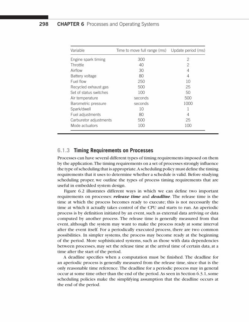
The engine controller takes a variety of inputs that determine the state of the engine.It then controls two basic engine parameters: the spark plug firings and the fuel/air mix-ture. The engine control is computed periodically, but the periods of the different inputs andoutputs range over several orders of magnitude of time. An early paper on automotive elec-tronics by Marley [Mar78] described the rates at which engine inputs and outputs must behandled.
298 CHAPTER 6 Processes and Operating Systems
Variable Time to move full range (ms) Update period (ms)
Engine spark timing 300 2Throttle 40 2Airflow 30 4Battery voltage 80 4Fuel flow 250 10Recycled exhaust gas 500 25Set of status switches 100 50Air temperature seconds 500Barometric pressure seconds 1000Spark/dwell 10 1Fuel adjustments 80 4Carburetor adjustments 500 25Mode actuators 100 100
6.1.3 Timing Requirements on ProcessesProcesses can have several different types of timing requirements imposed on themby the application.The timing requirements on a set of processes strongly influencethe type of scheduling that is appropriate.A scheduling policymust define the timingrequirements that it uses to determine whether a schedule is valid. Before studyingscheduling proper, we outline the types of process timing requirements that areuseful in embedded system design.
Figure 6.2 illustrates different ways in which we can define two importantrequirements on processes: release time and deadline. The release time is thetime at which the process becomes ready to execute; this is not necessarily thetime at which it actually takes control of the CPU and starts to run. An aperiodicprocess is by definition initiated by an event, such as external data arriving or datacomputed by another process. The release time is generally measured from thatevent, although the system may want to make the process ready at some intervalafter the event itself. For a periodically executed process, there are two commonpossibilities. In simpler systems, the process may become ready at the beginningof the period. More sophisticated systems, such as those with data dependenciesbetween processes,may set the release time at the arrival time of certain data, at atime after the start of the period.
A deadline specifies when a computation must be finished. The deadline foran aperiodic process is generally measured from the release time, since that is theonly reasonable time reference.The deadline for a periodic process may in generaloccur at some time other than the end of the period.As seen in Section 6.3.1, somescheduling policies make the simplifying assumption that the deadline occurs atthe end of the period.

6.1 Multiple Tasks and Multiple Processes 299
P1
Deadline
Release timeAperiodic process
Time
P1
Deadline
Release time
Periodic process initiated at start of period
Time
Period
P1
Deadline
Release time
Periodic process released by event
Time
Period
FIGURE 6.2
Example definitions of release times and deadlines.
Rate requirements are also fairly common. A rate requirement specifies howquickly processes must be initiated. The period of a process is the time betweensuccessive executions. For example, the period of a digital filter is defined by thetime interval between successive input samples.The process’s rate is the inverse ofits period. In a multirate system,each process executes at its own distinct rate.Themost common case for periodic processes is for the initiation interval to be equal tothe period. However,pipelined execution of processes allows the initiation intervalto be less than the period. Figure 6.3 illustrates process execution in a system withfour CPUs.The various execution instances of program P1 have been subscripted todistinguish their initiation times. In this case, the initiation interval is equal to one-fourth of the period. It is possible for a process to have an initiation rate less thanthe period even in single-CPU systems. If the process execution time is significantlyless than the period, it may be possible to initiate multiple copies of a program atslightly offset times.

300 CHAPTER 6 Processes and Operating Systems
P1i P1i14CPU 1
P1i11 P1i15CPU 2
P1i12 P1i16CPU 3
P1i13 P1i17CPU 4
Time
FIGURE 6.3
A sequence of processes with a high initiation rate.
What happenswhen a processmisses a deadline? The practical effects of a timingviolation depend on the application—the results can be catastrophic in an automo-tive control system,whereas a missed deadline in a multimedia systemmay cause anaudio or video glitch.The system can be designed to take a variety of actions whena deadline is missed. Safety-critical systems may try to take compensatory measuressuch as approximating data or switching into a special safety mode. Systems forwhich safety is not as important may take simple measures to avoid propagatingbad data, such as inserting silence in a phone line, or may completely ignore thefailure.
Even if the modules are functionally correct, their timing improper behaviorcan introduce major execution errors. Application Example 6.2 describes a timingproblem in space shuttle software that caused the delay of the first launch of theshuttle.
Application Example 6.2
A space shuttle software errorGarman [Gar81] describes a software problem that delayed the first launch of the U.S. spaceshuttle. No one was hurt and the launch proceeded after the computers were reset. However,this bug was serious and unanticipated.
The shuttle’s primary control system was known as the Primary Avionics Software System(PASS). It used four computers to monitor events, with the four machines voting to ensurefault tolerance. Four computers allowed one machine to fail while still leaving three operatingmachines to vote, such that a majority vote would still be possible to determine operating pro-cedures. If at least two machines failed, control was to be turned over to a fifth computer calledthe Backup Flight Control System (BFS). The BFS used the same computer, requirements,programming language, and compiler, but it was developed by a different organization thanthe one that built the PASS to ensure that methodological errors did not cause simultaneousfailure of both systems. The switchover from PASS to BFS was controlled by the astronauts.

6.1 Multiple Tasks and Multiple Processes 301
During normal operation, the BFS would listen to the operation of the PASS computers sothat it could keep track of the state of the shuttle. However, BFS would stop listening when itthought that PASS was compromising data fetching. This would prevent PASS failures frominadvertently destroying the state of the BFS. PASS used an asynchronous, priority-drivensoftware architecture. If high-priority processes take too much time, the OS can skip or delaylower-priority processing. The BFS, in contrast, used a time-slot system that allocated a fixedamount of time to each process. Since the BFS monitored the PASS, it could get confusedby temporary overloads on the primary system. As a result, the PASS was changed late in thedesign cycle to make its behavior more amenable to the backup system.
On the morning of the launch attempt, the BFS failed to synchronize itself with the primarysystem. It saw the events on the PASS system as inconsistent and therefore stopped listeningto PASS behavior. It turned out that all PASS and BFS processing had been running laterelative to telemetry data. This occurred because the system incorrectly calculated its starttime.
After much analysis of system traces and software, it was determined that a few minorchanges to the software had caused the problem. First, about 2 years before the incident,a subroutine used to initialize the data bus was modified. Since this routine was run prior tocalculating the start time, it introduced an additional, unnoticed delay into that computation.About a year later, a constant was changed in an attempt to fix that problem. As a result ofthese changes, there was a 1 in 67 probability for a timing problem. When this occurred,almost all computations on the computers would occur a cycle late, leading to the observedfailure. The problems were difficult to detect in testing since they required running through allthe initialization code; many tests start with a known configuration to save the time required torun the setup code. The changes to the programs were also not obviously related to the finalchanges in timing.
The order of execution of processes may be constrained when the processespass data between each other. Figure 6.4 shows a set of processes with data depen-dencies among them. Before a process can become ready,all the processes onwhichit depends must complete and send their data to it. The data dependencies definea partial ordering on process execution—P1 and P2 can execute in any order (orin interleaved fashion) but must both complete before P3, and P3 must completebefore P4.All processesmust finish before the end of the period.The data dependen-cies must form a directed acyclic graph (DAG)—a cycle in the data dependencies isdifficult to interpret in a periodically executed system.
A set of processes with data dependencies is known as a task graph. Althoughthe terminology for elements of a task graph varies from author to author,we willconsider a component of the task graph (a set of nodes connected by data depen-dencies) as a task and the complete graph as the task set . Figure 6.4 also showsa second task with two processes. The two tasks ({P1, P2, P3, P4} and {P5, P6})have no timing relationships between them.
Communication among processes that run at different rates cannot be repre-sented by data dependencies because there is no one-to-one relationship betweendata coming out of the source process and going into the destination process.

302 CHAPTER 6 Processes and Operating Systems
P1 P2
P3
P4
P5
P6
FIGURE 6.4
Data dependencies among processes.
System Video Audio
FIGURE 6.5
Communication among processes at different rates.
Nevertheless, communication among processes of different rates is very common.Figure 6.5 illustrates the communication required among three elements of anMPEG audio/video decoder. Data come into the decoder in the system format,which multiplexes audio and video data. The system decoder process demulti-plexes the audio and video data and distributes it to the appropriate processes.Multirate communication is necessarily one way—for example, the system pro-cess writes data to the video process, but a separate communication mechanismmust be provided for communication from the video process back to the systemprocess.
6.1.4 CPU MetricsWe also need some terminology to describe how the process actually executes.Theinitiation time is the time at which a process actually starts executing on the CPU.The completion time is the time at which the process finishes its work.
The most basic measure of work is the amount of CPU time expended bya process. The CPU time of process i is called Ci . Note that the CPU time is notequal to the completion time minus initiation time; several other processes mayinterrupt execution.The total CPU time consumed by a set of processes is

6.1 Multiple Tasks and Multiple Processes 303
T �∑
1� i�n
Ti . (6.1)
We need a basic measure of the efficiency with which we use the CPU. Thesimplest and most direct measure is utilization:
U �CPU time for useful work
total available CPU time. (6.2)
Utilization is the ratio of the CPU time that is being used for useful computationsto the total available CPU time. This ratio ranges between 0 and 1,with 1 meaningthat all of the available CPU time is being used for system purposes. The utilizationis often expressed as a percentage. If we measure the total execution time of allprocesses over an interval of time t , then the CPU utilization is
U �T
t. (6.3)
6.1.5 Process State and SchedulingThe first job of the OS is to determine that process runs next.The work of choosingthe order of running processes is known as scheduling.
The OS considers a process to be in one of three basic scheduling states:waiting, ready, or executing. There is at most one process executing on theCPU at any time. (If there is no useful work to be done, an idling process maybe used to perform a null operation.) Any process that could execute is in theready state; the OS chooses among the ready processes to select the next execut-ing process. A process may not, however, always be ready to run. For instance, aprocess may be waiting for data from an I/O device or another process, or it maybe set to run from a timer that has not yet expired. Such processes are in the wait-ing state. Figure 6.6 shows the possible transitions between states available to aprocess. A process goes into the waiting state when it needs data that it has notyet received or when it has finished all its work for the current period. A processgoes into the ready state when it receives its required data and when it entersa new period. A process can go into the executing state only when it has all itsdata, is ready to run, and the scheduler selects the process as the next processto run.
6.1.6 Some Scheduling PoliciesA scheduling policy defines how processes are selected for promotion from theready state to the running state. Every multitasking OS implements some type ofscheduling policy. Choosing the right scheduling policy not only ensures that thesystem will meet all its timing requirements,but it also has a profound influence onthe CPU horsepower required to implement the system’s functionality.

304 CHAPTER 6 Processes and Operating Systems
Executing
Ready
Chosento run
Gets data, CPU ready Needsdata
Needs data
Preempted
Received data Waiting
FIGURE 6.6
Scheduling states of a process.
Schedulability means whether there exists a schedule of execution for theprocesses in a system that satisfies all their timing requirements. In general,we mustconstruct a schedule to show schedulability, but in some cases we can eliminatesome sets of processes as unschedulable using some very simple tests. Utilizationis one of the key metrics in evaluating a scheduling policy. Our most basic require-ment is that CPU utilization be no more than 100% since we can’t use the CPUmorethan 100% of the time.
When we evaluate the utilization of the CPU, we generally do so over a finiteperiod that covers all possible combinations of process executions. For periodicprocesses, the length of time that must be considered is the hyperperiod , whichis the least-common multiple of the periods of all the processes. (The completeschedule for the least-common multiple of the periods is sometimes called theunrolled schedule.) Ifwe evaluate the hyperperiod,we are sure to have consideredall possible combinations of the periodic processes.The next example evaluates theutilization of a simple set of processes.
Example 6.1
Utilization of a set of processesWe are given three processes, their execution times, and their periods:
Process Period Execution time
P1 1.0�10�3 1.0�10�4
P2 1.0�10�3 2.0�10�4
P3 5.0�10�3 3.0�10�4
The least common multiple of these periods is 5 � 10�3 s.

6.1 Multiple Tasks and Multiple Processes 305
In order to calculate the utilization, we have to figure out how many times each process isexecuted in one hyperperiod: P1 and P2 are each executed five times while P3 is executedonce.
We can now determine the utilization over the hyperperiod:
U �5.1� 10�4 � 5.2� 10�4 � 1.3� 10�4
5� 10�3� 0.36
This is well below our maximum utilization of 1.0.
We will see that some types of timing requirements for a set of processes implythat we cannot utilize 100% of the CPU’s execution time on useful work, evenignoring context switching overhead. However, some scheduling policies candeliver higher CPU utilizations than others, even for the same timing requirements.The best policy depends on the required timing characteristics of the processesbeing scheduled.
One very simple scheduling policy is known as cyclostatic scheduling or some-times as Time Division Multiple Access scheduling. As illustrated in Figure 6.7,a cyclostatic schedule is divided into equal-sized time slots over an interval equalto the length of the hyperperiod H . Processes always run in the same time slot.Two factors affect utilization: the number of time slots used and the fraction of eachtime slot that is used for useful work. Depending on the deadlines for some of theprocesses,we may need to leave some time slots empty.And since the time slots areof equal size,some short processes may have time left over in their time slot.We canuse utilization as a schedulability measure: the total CPU time of all the processesmust be less than the hyperperiod.
Another scheduling policy that is slightly more sophisticated is round robin.Asillustrated in Figure 6.8, round robin uses the same hyperperiod as does cyclostatic.It also evaluates the processes in order. But unlike cyclostatic scheduling,if a process
P1 P2 P3
H
P1 P2 P3
H
FIGURE 6.7
Cyclostatic scheduling.
H
P3P2P2P1 P3
H
FIGURE 6.8
Round-robin scheduling.

306 CHAPTER 6 Processes and Operating Systems
does not have any useful work to do, the round-robin scheduler moves on to thenext process in order to fill the time slot with useful work. In this example, allthree processes execute during the first hyperperiod, but during the second one,P1 has no useful work and is skipped. The processes are always evaluated in thesame order.The last time slot in the hyperperiod is left empty;if we have occasional,non-periodic tasks without deadlines, we can execute them in these empty timeslots. Round-robin scheduling is often used in hardware such as buses because it isvery simple to implement but it provides some amount of flexibility.
In addition to utilization, we must also consider scheduling overhead—theexecution time required to choose the next execution process,which is incurred inaddition to any context switching overhead. In general, the more sophisticated thescheduling policy,themore CPU time it takes during system operation to implementit. Moreover, we generally achieve higher theoretical CPU utilization by applyingmore complex scheduling policies with higher overheads. The final decision ona scheduling policy must take into account both theoretical utilization and practicalscheduling overhead.
6.1.7 Running Periodic ProcessesWe need to find a programming technique that allows us to run periodic processes,ideally at different rates. For the moment, let’s think of a process as a subroutine;wewill call them p1( ), p2( ), etc. for simplicity. Our goal is to run these subroutines atrates determined by the system designer.
Here is a very simple program that runs our process subroutines repeatedly:
while (TRUE) {p1();p2();}
This program has several problems. First, it does not control the rate at whichthe processes execute—the loop runs as quickly as possible,starting a new iterationas soon as the previous iteration has finished. Second, all the processes run at thesame rate.
Before worrying about multiple rates, let’s first make the processes run at a con-trolled rate. One could imagine controlling the execution rate by carefully designingthe code—by determining the execution time of the instructions executed duringan iteration, we could pad the loop with useless operations (NOPs) to make theexecution time of an iteration equal to the desired period. Although some videogames were designed this way in the 1970s, this technique should be avoided.Modern processors make it hard to accurately determine execution time,as we sawin Chapter 5. Conditionals anywhere in the program make it even harder to besure that the loop consumes the same amount of execution time on every iteration.Furthermore, if any part of the program is changed, the entire timing scheme mustbe re-evaluated.

6.1 Multiple Tasks and Multiple Processes 307
A timer is a much more reliable way to control execution of the loop.We wouldprobably use the timer to generate periodic interrupts. Let’s assume for the momentthat the pall( ) function is called by the timer’s interrupt handler. Then this codewill execute each process once after a timer interrupt:
void pall() {p1();p2();}
Butwhat happenswhen a process runs too long? The timer’s interruptwill causethe CPU’s interrupt system tomask its interrupts,so the interruptwill not occur untilafter the pall( ) routine returns. As a result, the next iteration will start late.This is aserious problem,butwewill have towait for further refinements beforewe can fix it.
Our next problem is to execute different processes at different rates. If we haveseveral timers,we can set each timer to a different rate.We could then use a functionto collect all the processes that run at that rate:
void pA() {/* processes that run at rate A*/p1();p3();}
void pB() {/* processes that run at rate B */p2();p4();p5();}
This works, but it does require multiple timers, and we may not have enoughtimers to support all the rates required by a system.
An alternative is to use counters to divide the counter rate. If, for example,process p2() must run at 1/3 the rate of p1(), then we can use this code:
static int p2count = 0; /* use this to remember count acrosstimer interrupts */
void pall() {p1();if (p2count >= 2) { /* execute p2() and reset count */
p2();p2count = 0;}
else p2count++; /* just update count in this case */}

308 CHAPTER 6 Processes and Operating Systems
This solution allows us to execute processes at rates that are simple multiples ofeach other. However, when the rates aren’t related by a simple ratio, the countingprocess becomes more complex and more likely to contain bugs.
We have developed somewhat more reliable code,but this programming style isstill limited in capability and prone to bugs. To improve both the capabilities andreliability of our systems,we need to invent the RTOS.
6.2 PREEMPTIVE REAL-TIME OPERATING SYSTEMSA RTOS executes processes based upon timing constraints provided by the systemdesigner. The most reliable way to meet timing constraints accurately is to build apreemptive OS and to use priorities to control what process runs at any giventime.We will use these two concepts to build up a basic RTOS.We will use as ourexample OS FreeRTOS.org [Bar07]. This operating system runs on many differentplatforms.
6.2.1 PreemptionPreemption is an alternative to the C function call as a way to control execution.Tobe able to take full advantage of the timer,we must change our notion of a processas something more than a function call.We must, in fact, break the assumptions ofour high-level programming language.We will create new routines that allow us tojump from one subroutine to another at any point in the program. That, togetherwith the timer,will allow us to move between functions whenever necessary basedupon the system’s timing constraints.
We want to share the CPU across two processes. The kernel is the part ofthe OS that determines what process is running. The kernel is activated periodi-cally by the timer. The length of the timer period is known as the time quantumbecause it is the smallest increment in which we can control CPU activity. Thekernel determines what process will run next and causes that process to run. Onthe next timer interrupt, the kernel may pick the same process or another processto run.
Note that this use of the timer is very different from our use of the timer in thelast section. Before, we used the timer to control loop iterations, with one loop

6.2 Preemptive Real-Time Operating Systems 309
iteration including the execution of several complete processes. Here, the timequantum is in general smaller than the execution time of any of the processes.
How do we switch between processes before the process is done? We cannotrely on C-level mechanisms to do so. We can, however, use assembly language toswitch between processes. The timer interrupt causes control to change from thecurrently executing process to the kernel; assembly language can be used to saveand restore registers.We can similarly use assembly language to restore registers notfrom the process that was interrupted by the timer but to use registers from anyprocess we want. The set of registers that define a process are known as its con-text and switching from one process’s register set to another is known as contextswitching. The data structure that holds the state of the process is known as theprocess control block.
6.2.2 PrioritiesHow does the kernel determine what process will run next?We want a mechanismthat executes quickly so that we don’t spend all our time in the kernel and starve outthe processes that do the useful work. If we assign each task a numerical priority,then the kernel can simply look at the processes and their priorities,see which onesactuallywant to execute (somemay bewaiting for data or for some event),and selectthe highest priority process that is ready to run. This mechanism is both flexibleand fast.The priority is a non-negative integer value.The exact value of the priorityis not as important as the relative priority of different processes. In this book, wewill generally use priority 1 as the highest priority,but it is equally reasonable to use1 or 0 as the lowest priority value (as FreeRTOS.org does).
Example 6.2 shows how priorities can be used to schedule processes.
Example 6.2
Priority-driven schedulingFor this example, we will adopt the following simple rules:
■ Each process has a fixed priority that does not vary during the course of execution.(More sophisticated scheduling schemes do, in fact, change the priorities of processesto control what happens next.)
■ The ready process with the highest priority (with 1 as the highest priority of all) is selectedfor execution.

310 CHAPTER 6 Processes and Operating Systems
■ A process continues execution until it completes or it is preempted by a higher-priorityprocess.
Let’s define a simple system with three processes as seen below.
Process Priority Execution time
P1 1 10P2 2 30P3 3 20
In addition to describing the properties of the processes in general, we need to know theenvironmental setup. We assume that P2 is ready to run when the system is started, P1 isreleased at time 15, and P3 is released at time 18.
Once we know the process properties and the environment,we can use the pri-orities to determine which process is running throughout the complete executionof the system.
0 10 20 30 40 50 60
P2 P2P1 P3
P2 release
P1 release
P3 release
When the system begins execution,P2 is the only ready process, so it is selectedfor execution. At time 15, P1 becomes ready; it preempts P2 and begins executionsince it has a higher priority. Since P1 is the highest-priority process in the system,it is guaranteed to execute until it finishes. P3’s data arrive at time 18,but it cannotpreempt P1. Even when P1 finishes, P3 is not allowed to run. P2 is still ready andhas higher priority than P3. Only after both P1 and P2 finish can P3 execute.
6.2.3 Processes and ContextThe best way to understand processes and context is to dive into an RTOS imple-mentation. We will use the FreeRTOS.org kernel as an example; in particular,we will use version 4.7.0 for the ARM7 AT91 platform. A process is known inFreeRTOS.org as a task. Task priorities in FreeRTOS.org are ranked opposite tothe convention we use in the rest of the book: higher numbers denote higherpriorities and the priority 0 task is the idle task.

6.2 Preemptive Real-Time Operating Systems 311
timer vPreemptiveTick portSAVE_CONTEXT portRESTORE_CONTEXT vTaskSwitchContext task 1 task 2
FIGURE 6.9
Sequence diagram for freeRTOS.org context switch.
To understand the basics of a context switch, let’s assume that the set of tasks isin steady state: Everything has been initialized, the OS is running, and we are readyfor a timer interrupt. Figure 6.9 shows a sequence diagram for a context switch infreeRTOS.org.This diagram shows the application tasks, the hardware timer, and allthe functions in the kernel that are involved in the context switch:
■ vPreemptiveTick() is called when the timer ticks.
■ portSAVE_CONTEXT() swaps out the current task context.
■ vTaskSwitchContext ( ) chooses a new task.
■ portRESTORE_CONTEXT() swaps in the new context.
Here is the code for vPreemptiveTick() in the file portISR.c:
void vPreemptiveTick( void ){
/* Save the context of the interrupted task. */portSAVE_CONTEXT();
/* WARNING - Do not use local (stack) variables here.Use globals if you must! */
static volatile unsigned portLONG ulDummy;
/* Clear tick timer interrupt indication. */ulDummy = portTIMER_REG_BASE_PTR->TC_SR;/* Increment the RTOS tick count, then look for the
highest priority task that is ready to run. */vTaskIncrementTick();vTaskSwitchContext();

312 CHAPTER 6 Processes and Operating Systems
/* Acknowledge the interrupt at AIC level... */AT91C_BASE_AIC->AIC_EOICR = portCLEAR_AIC_INTERRUPT;
/* Restore the context of the new task. */portRESTORE_CONTEXT();
}
vPreemptiveTick() has been declared as a naked function; this means that itdoes not use the normal procedure entry and exit code that is generated by thecompiler. Because the function is naked , the registers for the process that wasinterrupted are still available; vPreemptiveTick() doesn’t have to go to the proce-dure call stack to get their values. This is particularly handy since the proceduremechanism would save only part of the process state,making the state-saving codea little more complex.
The first thing that this routine must do is save the context of the task thatwas interrupted.To do this, it uses the routine portSAVE_CONTEXT(),which savesall the context of the stack. It then performs some housekeeping, such as incre-menting the tick count.The tick count is the internal timer that is used to determinedeadlines.After the tick is incremented, some tasks may have become ready as theypassed their deadlines.
Next, the OS determines which task to run next using the routinevTaskSwitchContext(). After some more housekeeping, it uses portRESTORE_CONTEXT() to restore the context of the task that was selected byvTaskSwitchContext(). The action of portRESTORE_CONTEXT() causes controlto transfer to that task without using the standard C return mechanism.
The code for portSAVE_CONTEXT(), in the file portmacro.h, is defined as amacro and not as a C function. It is structured in this way so that it doesn’t dis-turb the register values that need to be saved. Because it is a macro, it has to bewritten in a hard-to-read way—all code must be on the same line or end-of-linecontinuations (back slashes) must be used. Here is the code in more readable form,with the end-of-line continuations removed and the assembly language that is theheart of this routine temporarily removed.:
#define portSAVE_CONTEXT(){extern volatile void * volatile pxCurrentTCB;extern volatile unsigned portLONG ulCriticalNesting;
/* Push R0 as we are going to use the register. */asm volatile( /* assembly language code here */ );( void ) ulCriticalNesting;( void ) pxCurrentTCB;
}
The asm statement allows assembly language code to be introduced in-line intothe C program.The keyword volatile tells the compiler that the assembly language

6.2 Preemptive Real-Time Operating Systems 313
may change register values,which means that many compiler optimizations cannotbe performed across the assembly language code. The code uses ulCriticalNestingand pxCurrentTCB simply to avoid compiler warnings about unused variables—the variables are actually used in the assembly code, but the compiler cannotsee that.
The asm statement requires that the assembly language be entered as strings,one string per line, which makes the code hard to read. The fact that the code isincluded in a #define makes it even harder to read. Here is a cleaned-up version ofthe assembly language code from the asm volatile( ) statement:
STMDB SP!, {R0}/* Set R0 to point to the task stack pointer. */STMDB SP, {SP}^NOPSUB SP, SP, #4LDMIA SP!,{R0}/* Push the return address onto the stack. */STMDB R0!, {LR}/* Now we have saved LR we can use it instead of R0. */MOV LR, R0/* Pop R0 so we can save it onto the system mode stack. */LDMIA SP!, {R0}/* Push all the system mode registers onto the task
stack. */STMDB LR,{R0-LR}^NOPSUB LR, LR, #60 /*Push the SPSR onto the task stack. */MRS R0, SPSRSTMDB LR!, {R0}LDR R0, =ulCriticalNestingLDR R0, [R0]STMDB LR!, {R0}/*Store the new top of stack for the task. */LDR R0, =pxCurrentTCBLDR R0, [R0]STR LR, [R0]
Here is the code for vTaskSwitchContext( ),which is defined in the file tasks.c:
void vTaskSwitchContext( void ){
if( uxSchedulerSuspended != ( unsigned portBASE_TYPE )pdFALSE )

314 CHAPTER 6 Processes and Operating Systems
{/* The scheduler is currently suspended - do not
allow a context switch. */xMissedYield = pdTRUE;
return;}
/* Find the highest priority queue that contains readytasks. */
while( listLIST_IS_EMPTY(&( pxReadyTasksLists[uxTopReadyPriority ]) ) )
{––uxTopReadyPriority;
}
/* listGET_OWNER_OF_NEXT_ENTRY walks through the list,so the tasks of the same priority get an equal shareof the processor time. */
listGET_OWNER_OF_NEXT_ENTRY( pxCurrentTCB,&(pxReadyTasksLists[uxTopReadyPriority ] ) );vWriteTraceToBuffer();
}
This function is relatively straightforward—it walks down the list of tasks to iden-tify the highest-priority task. This function is designed to deterministically choosethe next task to run as long as the selected task is of equal or higher priority tothe interrupted task; the list of tasks that is checked is determined by the variableuxTopReadyPriority. Each list contains the set of processes with the same priority;once the proper priority has selected by determining the value of uxTopReadyPri-ority, the system rotates through processes of equal priority by walking downtheir list.
The portRESTORE_CONTEXT() routine is also defined in portmacro.h and isimplemented as a macro with embedded assembly language. Here is the macrowith the line continuations and assembly language code removed:
#define portRESTORE_CONTEXT(){extern volatile void * volatilepxCurrentTCB;extern volatile unsigned portLONGulCriticalNesting;
/* Set the LR to the task stack. */asm volatile (/* assembly language code here */);

6.2 Preemptive Real-Time Operating Systems 315
( void ) ulCriticalNesting;( void ) pxCurrentTCB;
}
Here is the assembly language code for portRESTORE_CONTEXT:
LDR R0, =pxCurrentTCBLDR R0, [R0]LDR LR, [R0]/* The critical nesting depth is the first item on the
stack. *//* Load it into the ulCriticalNesting variable. */LDR R0, =ulCriticalNestingLDMFD LR!, {R1}STR R1, [R0]/* Get the SPSR from the stack. */LDMFD LR!, {R0}MSR SPSR, R0/* Restore all system mode registers for the task. */LDMFD LR, {R0-R14}̂NOP/* Restore the return address. */LDR LR, [LR, #+60]/* And return - correcting the offset in the LR to obtain
the *//* correct address. */SUBS PC, LR, #4
6.2.4 Processes and Object-Oriented DesignWe need to design systems with processes as components. In this section,we sur-vey the ways we can describe processes in UML and how to use processes ascomponents in object-oriented design.
UML often refers to processes as active objects, that is, objects that have inde-pendent threads of control. The class that defines an active object is known as anactive class. Figure 6.10 shows an example of a UML active class. It has all thenormal characteristics of a class, including a name,attributes,and operations. It alsoprovides a set of signals that can be used to communicate with the process.A signalis an object that is passed between processes for asynchronous communication.Wedescribe signals in more detail in Section 6.2.4.
We can mix active objects and normal objects when describing a system.Figure 6.11 shows a simple collaboration diagram in which an object is used asan interface between two processes: p1 uses the w object to manipulate its databefore the data is sent to themaster process.

316 CHAPTER 6 Processes and Operating Systems
processClass 1
myAttributes
myOperations( )
Signals
start
resume
FIGURE 6.10
An active class in UML.
p1: processClass1
master: masterClass
w: wrapperClass ahat: fullMsga: rawMsg
FIGURE 6.11
A collaboration diagram with active and normal objects.
6.3 PRIORITY-BASED SCHEDULINGNow that we have a priority-based context switching mechanism, we have todetermine an algorithm by which to assign priorities to processes. After assign-ing priorities, the OS takes care of the rest by choosing the highest-priority readyprocess. There are two major ways to assign priorities:static priorities that do notchange during execution and dynamic priorities that do change. We will look atexamples of each in this section.
6.3.1 Rate-Monotonic SchedulingRate-monotonic scheduling (RMS), introduced by Liu and Layland [Liu73],wasone of the first scheduling policies developed for real-time systems and is still verywidely used. RMS is a static scheduling policy. It turns out that these fixed prioritiesare sufficient to efficiently schedule the processes in many situations.
The theory underlying RMS is known as rate-monotonic analysis (RMA).Thistheory, as summarized below,uses a relatively simple model of the system.
■ All processes run periodically on a single CPU.
■ Context switching time is ignored.

6.3 Priority-Based Scheduling 317
■ There are no data dependencies between processes.
■ The execution time for a process is constant.
■ All deadlines are at the ends of their periods.
■ The highest-priority ready process is always selected for execution.
The major result of RMA is that a relatively simple scheduling policy is opti-mal under certain conditions. Priorities are assigned by rank order of period,withthe process with the shortest period being assigned the highest priority. Thisfixed-priority scheduling policy is the optimum assignment of static priorities toprocesses, in that it provides the highest CPU utilization while ensuring that allprocesses meet their deadlines.
Example 6.3 illustrates RMS.
Example 6.3
Rate-monotonic schedulingHere is a simple set of processes and their characteristics.
Process Execution time Period
P1 1 4P2 2 6P3 3 12
Applying the principles of RMA, we give P1 the highest priority, P2 the middle priority,and P3 the lowest priority. To understand all the interactions between the periods, we need toconstruct a time line equal in length to hyperperiod, which is 12 in this case.
0 2 4 6 8 10 12
Time
P1
P2
P3
All three periods start at time zero. P1’s data arrive first. Since P1 is the highest-priorityprocess, it can start to execute immediately. After one time unit, P1 finishes and goes outof the ready state until the start of its next period. At time 1, P2 starts executing as the

318 CHAPTER 6 Processes and Operating Systems
highest-priority ready process. At time 3, P2 finishes and P3 starts executing. P1’s next iterationstarts at time 4, at which point it interrupts P3. P3 gets onemore time unit of execution betweenthe second iterations of P1 and P2, but P3 does not get to finish until after the third iterationof P1.
Consider the following different set of execution times for these processes, keeping thesame deadlines.
Process Execution time Period
P1 2 4P2 3 6P3 3 12
In this case, we can show that there is no feasible assignment of priorities that guaranteesscheduling. Even though each process alone has an execution time significantly less than itsperiod, combinations of processes can require more than 100% of the available CPU cycles.For example, during one 12 time-unit interval, we must execute P1 three times, requiring6 units of CPU time; P2 twice, costing 6 units of CPU time; and P3 one time, requiring 3 unitsof CPU time. The total of 6 + 6 + 3 = 15 units of CPU time is more than the 12 time unitsavailable, clearly exceeding the available CPU capacity.
Liu and Layland [Liu73] proved that the RMA priority assignment is optimalusing critical-instant analysis. We define the response time of a process as thetime at which the process finishes. The critical instant for a process is definedas the instant during execution at which the task has the largest response time. Itis easy to prove that the critical instant for any process P, under the RMA model,occurs when it is ready and all higher-priority processes are also ready—if wechange any higher-priority process to waiting, then P’s response time can only godown.
We can use critical-instant analysis to determine whether there is any feasibleschedule for the system. In the case of the second set of execution times inExample 6.3,therewas no feasible schedule. Critical-instant analysis also implies thatpriorities should be assigned in order of periods. Let the periods and computationtimes of two processes P1 and P2 be �1, �2 and T1, T2, with �1 < �2. We cangeneralize the result of Example 6.3 to show the total CPU requirements for thetwo processes in two cases. In the first case, let P1 have the higher priority. In theworst case we then execute P2 once during its period and as many iterations of P1as fit in the same interval. Since there are ��2/�1� iterations of P1 during a singleperiod of P2, the required constraint on CPU time, ignoring context switchingoverhead, is
⌊�2
�1
⌋T1 � T2 � �2. (6.4)

6.3 Priority-Based Scheduling 319
If, on the other hand,we give higher priority to P2, then critical-instant analysistells us that we must execute all of P2 and all of P1 in one of P1’s periods in theworst case:
T1 � T2 � �1. (6.5)
There are cases where the first relationship can be satisfied and the secondcannot, but there are no cases where the second relationship can be satisfied andthe first cannot.We can inductively show that the process with the shorter periodshould always be given higher priority for process sets of arbitrary size. It is alsopossible to prove that RMS always provides a feasible schedule if such a scheduleexists.
The bad news is that,although RMS is the optimal static-priority schedule,it doesnot always allow the system to use 100% of the available CPU cycles. In the RMSframework, the total CPU utilization for a set of n tasks is
U �n∑i�1
Ti�i
. (6.6)
The fraction Ti/�i is the fraction of time that the CPU spends executing task i.It is possible to show that for a set of two tasks under RMS scheduling, the CPUutilization U will be no greater than 2(21/2 � 1) ∼� 0.83. In other words, the CPUwill be idle at least 17% of the time. This idle time is due to the fact that prioritiesare assigned statically; we see in the next section that more aggressive schedulingpolicies can improve CPU utilization.When there are m tasks with fixed priorities,the maximum processor utilization is
U � m(21/m � 1). (6.7)
As m approaches infinity, the least upper bound to CPU utilization is ln 2 �0.69—the CPU will be idle 31% of the time. This does not mean that we can neveruse 100% of the CPU. If the periods of the tasks are arranged properly, then we canschedule tasks to make use of 100% of the CPU. But the least upper bound of 69%tells us that RMS can in some cases deliver utilizations significantly below 100%.
The implementation of RMS is very simple. Figure 6.12 shows C code for anRMS scheduler run at the OS’s timer interrupt. The code merely scans through thelist of processes in priority order and selects the highest-priority ready processto run. Because the priorities are static, the processes can be sorted by priorityin advance before the system starts executing. As a result, this scheduler has anasymptotic complexity of O(n),where n is the number of processes in the system.(This code assumes that processes are not created dynamically. If dynamic processcreation is required, the array can be replaced by a linked list of processes, butthe asymptotic complexity remains the same.) The RMS scheduler has both lowasymptotic complexity and low actual execution time, which helps minimize thediscrepancies between the zero-context-switch assumption of RMA and the actualexecution of an RMS system.

320 CHAPTER 6 Processes and Operating Systems
/* processes[] is an array of process activation records, stored in order of priority, with processes[0] being the highest-priority process */Activation_record processes[NPROCESSES];
void RMA(int current) { /* current � currently executing process */ int i; /* turn off current process (may be turned back on) */ processes[current].state � READY_STATE; /* find process to start executing */ for (i � 0; i < NPROCESSES; i��) if (processes[i].state �� READY_STATE) {
/* make this the running process */ processes[i].state �� EXECUTING_STATE; break; }}
FIGURE 6.12
C code for rate-monotonic scheduling.
6.3.2 Earliest-Deadline-First SchedulingEarliest deadline first (EDF) is another well-known scheduling policy that wasalso studied by Liu and Layland [Liu73]. It is a dynamic priority scheme—it changesprocess priorities during execution based on initiation times. As a result, it canachieve higher CPU utilizations than RMS.
The EDF policy is also very simple: It assigns priorities in order of deadline. Thehighest-priority process is the one whose deadline is nearest in time,and the lowest-priority process is the one whose deadline is farthest away. Clearly, priorities mustbe recalculated at every completion of a process. However, the final step of the OSduring the scheduling procedure is the same as for RMS—the highest-priority readyprocess is chosen for execution.
Example 6.4 illustrates EDF scheduling in practice.
Example 6.4
Earliest-deadline-first schedulingConsider the following processes:
Process Execution time Period
P1 1 3
P2 1 4
P3 2 5
The hyperperiod is 60. In order to be able to see the entire period, we write it as a table:

6.3 Priority-Based Scheduling 321
Time Running process Deadlines
0 P11 P22 P3 P13 P3 P24 P1 P35 P2 P16 P17 P3 P28 P3 P19 P1 P310 P211 P3 P1, P212 P113 P314 P2 P1, P315 P1 P216 P217 P3 P118 P119 P3 P2, P320 P2 P121 P122 P323 P3 P1, P224 P1 P325 P226 P3 P127 P1 P228 P329 P2 P1, P330 idle31 P1 P232 P3 P133 P334 P1 P335 P2 P1, P236 P137 P238 P3 P139 P3 P2, P340 P1
(Continued)

322 CHAPTER 6 Processes and Operating Systems
Time Running process Deadlines
41 P2 P142 P143 P3 P244 P3 P1, P345 P146 P247 P3 P1, P248 P349 P1 P350 P2 P151 P1 P252 P353 P3 P154 P2 P355 P1 P256 P2 P157 P158 P359 P3 P1, P2, P3
There is one time slot left at t � 30, giving a CPU utilization of 59/60.
Liu and Layland showed that EDF can achieve 100% utilization.A feasible sched-ule exists if the CPU utilization (calculated in the same way as for RMA) is�1.Theyalso showed that when an EDF system is overloaded and misses a deadline, it willrun at 100% capacity for a time before the deadline is missed.
The implementation of EDF is more complex than the RMS code. Figure 6.13outlines one way to implement EDF. The major problem is keeping the processessorted by time to deadline—since the times to deadlines for the processes changeduring execution, we cannot presort the processes into an array, as we could forRMS. To avoid resorting the entire set of records at every change, we can build abinary tree to keep the sorted records and incrementally update the sort.At the endof each period,we canmove the record to its new place in the sorted list by deletingit from the tree and then adding it back to the tree using standard tree manipulationtechniques. We must update process priorities by traversing them in sorted order,so the incremental sorting routines must also update the linked list pointers that letus traverse the records in deadline order. (The linked list lets us avoid traversing thetree to go from one node to another,which would require more time.) After puttingin the effort to building the sorted list of records, selecting the next executingprocess is done in a manner similar to that of RMS. However, the dynamic sortingadds complexity to the entire scheduling process. Each update of the sorted list

6.3 Priority-Based Scheduling 323
Deadline_tree
Activation_record
Data structure
Code
Activation_record
......
/* linked list, sorted by deadline */
Activation_record *processes;
/* data structure for sorting processes */
Deadline_tree *deadlines;
void expired_deadline(Activation_record *expired){
remove(expired); /* remove from the deadline-sorted list */
add(expired,expired->deadline); /* add at new deadline */
}
Void EDF(int current) { /* current � currently executing process */
int i;
/* turn off current process (may be turned back on) */
processes->state � READY_STATE;
/* find process to start executing */
for (alink = processes; alink !� NULL; alink � alink->next_deadline)
if (processes->state �� READY_STATE) {
/* make this the running process */
processes->state �� EXECUTING_STATE;
break;
}
}
FIGURE 6.13
C code for earliest-deadline-first scheduling.
requires O(log n) steps. The EDF code is also significantly more complex than theRMS code.
6.3.3 RMS vs. EDFWhich scheduling policy is better:RMS or EDF?That depends on your criteria. EDFcan extract higher utilization out of the CPU,but it may be difficult to diagnose thepossibility of an imminent overload. Because the scheduler does take some overheadtomake scheduling decisions,a factor that is ignored in the schedulability analysis ofboth EDF and RMS, running a scheduler at very high utilizations is somewhat prob-lematic. RMS achieves lower CPU utilization but is easier to ensure that all deadlines

324 CHAPTER 6 Processes and Operating Systems
will be satisfied. In some applications, it may be acceptable for some processes tooccasionally miss deadlines. For example, a set-top box for video decoding is nota safety-critical application, and the occasional display artifacts caused by missingdeadlines may be acceptable in some markets.
What if your set of processes is unschedulable and you need to guarantee thatthey complete their deadlines? There are several possibleways to solve this problem:
■ Get a faster CPU. That will reduce execution times without changing theperiods, giving you lower utilization. This will require you to redesign thehardware, but this is often feasible because you are rarely using the fastestCPU available.
■ Redesign the processes to take less execution time. This requires knowledgeof the code and may or may not be possible.
■ Rewrite the specification to change the deadlines. This is unlikely to befeasible,but may be in a few cases where some of the deadlines were initiallymade tighter than necessary.
6.3.4 A Closer Look at Our Modeling AssumptionsOur analyses of RMS and EDF have made some strong assumptions. These assump-tions have made the analyses much more tractable, but the predictions of analysismay not hold up in practice. Since a misprediction may cause a system to missa critical deadline, it is important to at least understand the consequences of theseassumptions.
In all of the above discussions,we have assumed that each process is totally self-contained. However, that is not always the case—for instance, a process may needa system resource,such as an I/O device or the bus,to complete its work. Schedulingthe processes without considering the resources those processes require can causepriority inversion, in which a low-priority process blocks execution of a higher-priority process by keeping hold of its resource. Example 6.5 illustrates priorityinversion.
Example 6.5
Priority inversionConsider a system with two processes: the higher-priority P1 and the lower-priority P2. Eachuses the microprocessor bus to communicate to peripherals. When P2 executes, it requeststhe bus from the operating system and receives it. If P1 becomes ready while P2 is using thebus, the OS will preempt P2 for P1, leaving P2 with control of the bus. When P1 requests thebus, it will be denied the bus, since P2 already owns it. Unless P1 has a way to take the busfrom P2, the two processes may deadlock.
The most common method for dealing with priority inversion is to promote thepriority of any process when it requests a resource from the OS.The priority of theprocess temporarily becomes higher than that of any other process that may use

6.4 Interprocess Communication Mechanisms 325
the resource.This ensures that the process will continue executing once it has theresource so that it can finish its work with the resource, return it to the OS, andallow other processes to use it. Once the process is finished with the resource, itspriority is demoted to its normal value. Several methods have been developed tomanage the priority swapping process [Liu00].
Rate-monotonic scheduling assumes that there are no data dependenciesbetween processes. Example 6.6 shows that knowledge of data dependencies canhelp use the CPU more efficiently.
Example 6.6
Data dependencies and schedulingData dependencies imply that certain combinations of processes can never occur. Considerthe simple example [Yen98] below.
P2
P1 P3
1 2 1
2
10
8
Task graph
Task
Task rates
Deadline
P1
P2
2
1
P3 4
Process
Execution times
CPU time
We know that P1 and P2 cannot execute at the same time, since P1 must finish beforeP2 can begin. Furthermore, we also know that because P3 has a higher priority, it will notpreempt both P1 and P2 in a single iteration. If P3 preempts P1, then P3 will complete beforeP2 begins; if P3 preempts P2, then it will not interfere with P1 in that iteration. Because weknow that some combinations of processes cannot be ready at the same time, we know thatour worst-case CPU requirements are less than would be required if all processes could beready simultaneously.
6.4 INTERPROCESS COMMUNICATION MECHANISMSProcesses often need to communicate with each other. Interprocess communi-cation mechanisms are provided by the operating system as part of the processabstraction.

326 CHAPTER 6 Processes and Operating Systems
CPU
Write
Bus
I/O device
Read
Sharedlocation
Memory
FIGURE 6.14
Shared memory communication implemented on a bus.
In general, a process can send a communication in one of two ways: blockingor nonblocking. After sending a blocking communication, the process goes intothe waiting state until it receives a response. Nonblocking communication allowsthe process to continue execution after sending the communication. Both types ofcommunication are useful.
There are two major styles of interprocess communication: shared memoryandmessage passing.The two are logically equivalent—given one,you can buildan interface that implements the other. However, some programs may be easier towrite using one rather than the other. In addition, the hardware platform may makeone easier to implement or more efficient than the other.
6.4.1 Shared Memory CommunicationFigure 6.14 illustrates how shared memory communication works in a bus-basedsystem. Two components, such as a CPU and an I/O device, communicate througha shared memory location. The software on the CPU has been designed to knowthe address of the shared location;the shared location has also been loaded into theproper register of the I/O device. If, as in the figure, the CPU wants to send data tothe device, it writes to the shared location.The I/O device then reads the data fromthat location. The read and write operations are standard and can be encapsulatedin a procedural interface.
Example 6.7 describes the use of shared memory as a practical communicationmechanism.
Example 6.7
Elastic buffers as shared memoryThe text compressor of Application Example 3.4 provides a good example of a shared memory.As shown below, the text compressor uses the CPU to compress incoming text, which is thensent on a serial line by a UART.

6.4 Interprocess Communication Mechanisms 327
UART
Size info
CPUIn
UART
OutBuffer
Memory
The input data arrive at a constant rate and are easy to manage. But because the outputdata are consumed at a variable rate, these data require an elastic buffer. The CPU and outputUART share a memory area—the CPU writes compressed characters into the buffer and theUART removes them as necessary to fill the serial line. Because the number of bits in thebuffer changes constantly, the compression and transmission processes need additional sizeinformation. In this case, coordination is simple—the CPU writes at one end of the buffer andthe UART reads at the other end. The only challenge is to make sure that the UART does notoverrun the buffer.
As an application of sharedmemory,let us consider the situation of Figure 6.14 inwhich the CPU and the I/O device want to communicate through a shared memoryblock. There must be a flag that tells the CPU when the data from the I/O deviceis ready. The flag, an additional shared data location, has a value of 0 when the dataare not ready and 1 when the data are ready.The CPU, for example,would write thedata, and then set the flag location to 1. If the flag is used only by the CPU, then theflag can be implemented using a standard memory write operation. If the same flagis used for bidirectional signaling between the CPU and the I/O device, care mustbe taken. Consider the following scenario:
1. CPU reads the flag location and sees that it is 0.
2. I/O device reads the flag location and sees that it is 0.
3. CPU sets the flag location to 1 and writes data to the shared location.
4. I/O device erroneously sets the flag to 1 and overwrites the data left bythe CPU.
The above scenario is caused by a critical timing race between the two programs.To avoid such problems, the microprocessor bus must support an atomic test-and-set operation,which is available on a number of microprocessors. The test-and-setoperation first reads a location and then sets it to a specified value. It returns theresult of the test. If the location was already set, then the additional set has no effectbut the test-and-set instruction returns a false result. If the location was not set, the
328 CHAPTER 6 Processes and Operating Systems
instruction returns true and the location is in fact set. The bus supports this as anatomic operation that cannot be interrupted. Programming Example 6.1 describesa test-and-set operation in more detail.
A test-and-set can be used to implement a semaphore,which is a language-levelsynchronization construct. For the moment, let’s assume that the system providesone semaphore that is used to guard access to a block of protected memory. Anyprocess that wants to access the memory must use the semaphore to ensure that noother process is actively using it.As shown below,the semaphore names by traditionare P( ) to gain access to the protected memory andV( ) to release it.
/* some nonprotected operations here */P(); /* wait for semaphore *//* do protected work here */V(); /* release semaphore */
The P( ) operation uses a test-and-set to repeatedly test a location that holdsa lock on the memory block. The P( ) operation does not exit until the lock isavailable; once it is available, the test-and-set automatically sets the lock. Once pastthe P( ) operation, the process can work on the protected memory block. The V( )operation resets the lock, allowing other processes access to the region by usingthe P( ) function.
Programming Example 6.1
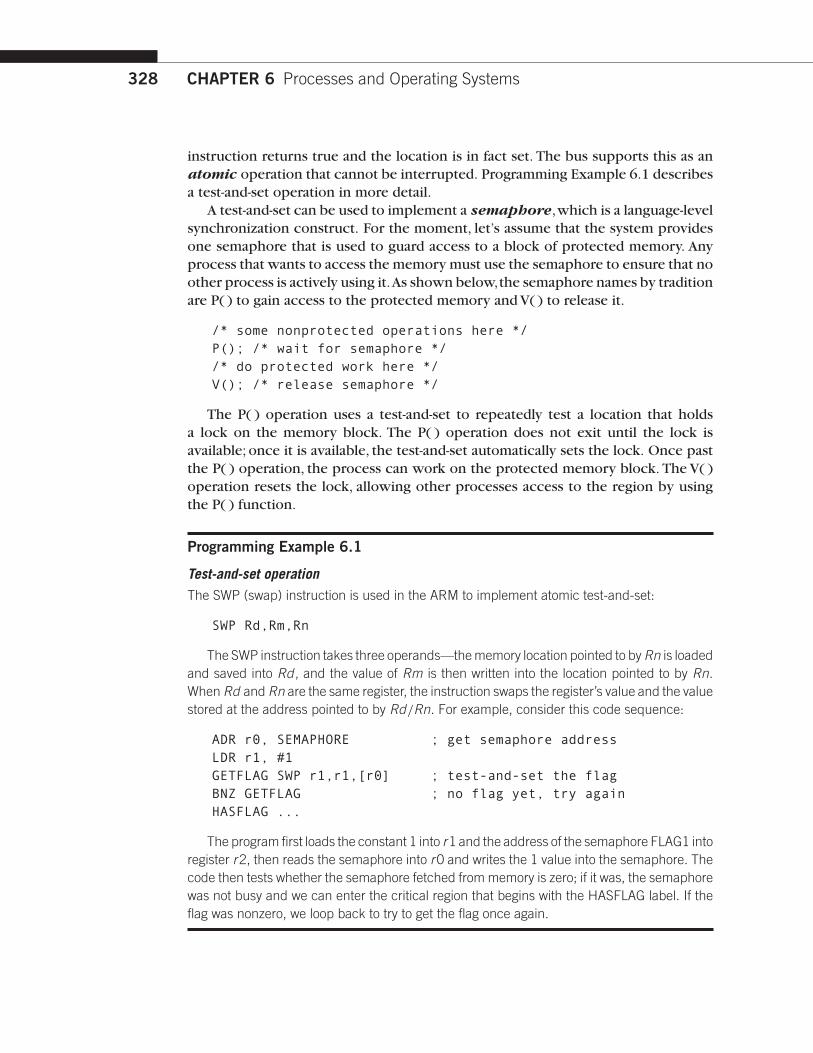
Test-and-set operationThe SWP (swap) instruction is used in the ARM to implement atomic test-and-set:
SWP Rd,Rm,Rn
The SWP instruction takes three operands—thememory location pointed to byRn is loadedand saved into Rd , and the value of Rm is then written into the location pointed to by Rn.WhenRd andRn are the same register, the instruction swaps the register’s value and the valuestored at the address pointed to by Rd/Rn. For example, consider this code sequence:
ADR r0, SEMAPHORE ; get semaphore addressLDR r1, #1GETFLAG SWP r1,r1,[r0] ; test-and-set the flagBNZ GETFLAG ; no flag yet, try againHASFLAG ...
The program first loads the constant 1 into r1 and the address of the semaphore FLAG1 intoregister r2, then reads the semaphore into r0 and writes the 1 value into the semaphore. Thecode then tests whether the semaphore fetched from memory is zero; if it was, the semaphorewas not busy and we can enter the critical region that begins with the HASFLAG label. If theflag was nonzero, we loop back to try to get the flag once again.
6.4 Interprocess Communication Mechanisms 329
msg msg
CPU 1 CPU 2
FIGURE 6.15
Message passing communication.
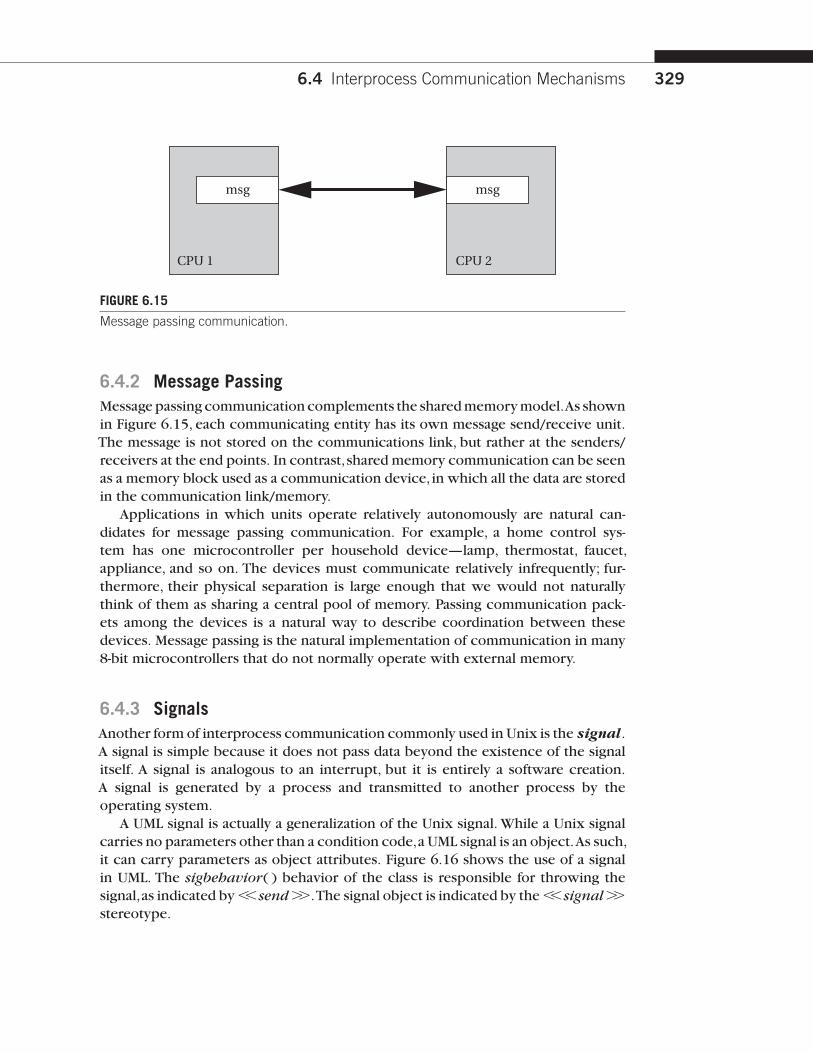
6.4.2 Message PassingMessagepassing communication complements the sharedmemorymodel.As shownin Figure 6.15, each communicating entity has its own message send/receive unit.The message is not stored on the communications link, but rather at the senders/receivers at the end points. In contrast,shared memory communication can be seenas a memory block used as a communication device, in which all the data are storedin the communication link/memory.
Applications in which units operate relatively autonomously are natural can-didates for message passing communication. For example, a home control sys-tem has one microcontroller per household device—lamp, thermostat, faucet,appliance, and so on. The devices must communicate relatively infrequently; fur-thermore, their physical separation is large enough that we would not naturallythink of them as sharing a central pool of memory. Passing communication pack-ets among the devices is a natural way to describe coordination between thesedevices. Message passing is the natural implementation of communication in many8-bit microcontrollers that do not normally operate with external memory.
6.4.3 SignalsAnother form of interprocess communication commonly used in Unix is the signal .A signal is simple because it does not pass data beyond the existence of the signalitself. A signal is analogous to an interrupt, but it is entirely a software creation.A signal is generated by a process and transmitted to another process by theoperating system.
A UML signal is actually a generalization of the Unix signal. While a Unix signalcarries no parameters other than a condition code,a UML signal is an object.As such,it can carry parameters as object attributes. Figure 6.16 shows the use of a signalin UML. The sigbehavior( ) behavior of the class is responsible for throwing thesignal,as indicated by��send��.The signal object is indicated by the��signal��stereotype.

330 CHAPTER 6 Processes and Operating Systems
<<signal>>aSig
p: integer
someClass
sigbehavior( )<<send>>
FIGURE 6.16
Use of a UML signal.
6.5 EVALUATING OPERATING SYSTEM PERFORMANCEThe scheduling policy does not tell us all that we would like to know about theperformance of a real system running processes. Our analysis of scheduling policiesmakes some simplifying assumptions:
■ We have assumed that context switches require zero time.Although it is oftenreasonable to neglect context switch time when it is much smaller than theprocess execution time, context switching can add significant delay in somecases.
■ We have assumed that we know the execution time of the processes. In fact,we learned in Section 5.6 that program time is not a single number, but canbe bounded by worst-case and best-case execution times.
■ We probably determined worst-case or best-case times for the processes inisolation. But,in fact,they interactwith eachother in the cache. Cache conflictsamong processes can drastically degrade process execution time.
The zero-time context switch assumption used in the analysis of RMS is notcorrect—we must execute instructions to save and restore context, and we mustexecute additional instructions to implement the scheduling policy. On the otherhand, context switching can be implemented efficiently—context switching neednot kill performance. The effects of nonzero context switching time must be care-fully analyzed in the context of a particular implementation to be sure that thepredictions of an ideal scheduling policy are sufficiently accurate.
Example 6.8 shows that context switching can, in fact, cause a system to miss adeadline.
Example 6.8
Scheduling and context switching overheadAppearing below is a set of processes and their characteristics.

6.5 Evaluating Operating System Performance 331
Process Execution time Deadline
P1 3 5P2 3 10
First, let us try to find a schedule assuming that context switching time is zero. Followingis a feasible schedule for a sequence of data arrivals that meets all the deadlines:
0 2
P1
P1 P2 P1
P2
4 6 8 10Time
Now let us assume that the total time to initiate a process, including context switchingand scheduling policy evaluation, is one time unit. It is easy to see that there is no feasibleschedule for the above release time sequence, since we require a total of 2TP1 � TP2 �2� (1� 3)� (1� 3) � 11 time units to execute one period of P2 and two periods of P1.
In Example 6.8,overhead was a large fraction of the process execution time andof the periods. In most real-time operating systems, a context switch requires onlya few hundred instructions,with only slightly more overhead for a simple real-timescheduler like RMS.When the overhead time is very small relative to the task periods,then the zero-time context switch assumption is often a reasonable approximation.Problems are most likely to manifest themselves in the highest-rate processes,whichare often themost critical in any case. Completely checking that all deadlines will bemet with nonzero context switching time requires checking all possible schedulesfor processes and including the context switch time at each preemption or processinitiation. However, assuming an average number of context switches per processand computing CPU utilization can provide at least an estimate of how close thesystem is to CPU capacity.
Another important assumption we have made thus far is that process executiontime is constant. As seen in Section 5.6, this is definitely not the case—both data-dependent behavior and caching effects can cause large variations in run times. Ifwe can determine worst-case execution time, then shorter run times for a processsimply mean unused CPU time. If we cannot accurately boundWCET, then we willbe left with a very conservative estimate of execution time that will leave evenmoreCPU time unused.

332 CHAPTER 6 Processes and Operating Systems
Wealso assumed that processes don’t interact,but the cache causes the executionof one program to influence the execution time of other programs.The techniquesfor bounding the cache-based performance of a single program do not work whenmultiple programs are in the same cache.Many real-time systemshave beendesignedbased on the assumption that there is no cache present, even though one actuallyexists. This grossly conservative assumption is made because the system architectslack tools that permit them to analyze the effect of caching. Since they do not knowwhere caching will cause problems, they are forced to retreat to the simplifyingassumption that there is no cache. The result is extremely overdesigned hardware,which has much more computational power than is necessary. However, just asexperience tells us that a well-designed cache provides significant performancebenefits for a single program,a properly sized cache can allow a microprocessor torun a set of processes much more quickly. By analyzing the effects of the cache,wecan make much better use of the available hardware.
Li and Wolf [Li99] developed amodel for estimating the performance of multipleprocesses sharing a cache. In the model, some processes can be given reservationsin the cache, such that only a particular process can inhabit a reserved section ofthe cache; other processes are left to share the cache. We generally want to usecache partitions only for performance-critical processes since cache reservationsare wasteful of limited cache space. Performance is estimated by constructing aschedule, taking into account not just execution time of the processes but alsothe state of the cache. Each process in the shared section of the cache is modeledby a binary variable: 1 if present in the cache and 0 if not. Each process is alsocharacterized by three total execution times: assuming no caching, with typicalcaching, and with all code always resident in the cache.The always-resident time isunrealistically optimistic, but it can be used to find a lower bound on the requiredschedule time. During construction of the schedule, we can look at the currentcache state to see whether the no-cache or typical-caching execution time shouldbe used at this point in the schedule.We can also update the cache state if the cacheis needed for another process.Although this model is simple,it provides muchmorerealistic performance estimates than assuming the cache either is nonexistent or isperfect. Example 6.9 shows how cache management can improve CPU utilization.
Example 6.9
Effects of scheduling on the cacheConsider a system containing the following three processes:
Process Worst-case CPU time Average-case CPU time
P1 8 6P2 4 3P3 4 3
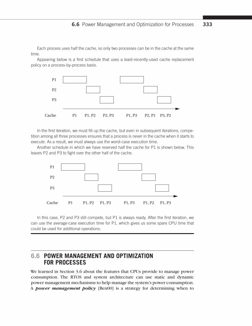
6.6 Power Management and Optimization for Processes 333
Each process uses half the cache, so only two processes can be in the cache at the sametime.
Appearing below is a first schedule that uses a least-recently-used cache replacementpolicy on a process-by-process basis.
P1
P1 P1, P2 P2, P3 P1, P3 P2, P1 P3, P2Cache
P2
P3
In the first iteration, we must fill up the cache, but even in subsequent iterations, compe-tition among all three processes ensures that a process is never in the cache when it starts toexecute. As a result, we must always use the worst-case execution time.
Another schedule in which we have reserved half the cache for P1 is shown below. Thisleaves P2 and P3 to fight over the other half of the cache.
P1
P1 P1, P2 P1, P3 P1, P3 P1, P2 P1, P3Cache
P2
P3
In this case, P2 and P3 still compete, but P1 is always ready. After the first iteration, wecan use the average-case execution time for P1, which gives us some spare CPU time thatcould be used for additional operations.
6.6 POWER MANAGEMENT AND OPTIMIZATIONFOR PROCESSES
We learned in Section 3.6 about the features that CPUs provide to manage powerconsumption. The RTOS and system architecture can use static and dynamicpower management mechanisms to help manage the system’s power consumption.A power management policy [Ben00] is a strategy for determining when to

334 CHAPTER 6 Processes and Operating Systems
perform certain power management operations. A power management policy ingeneral examines the state of the system to determine when to take actions.However, the overall strategy embodied in the policy should be designed basedon the characteristics of the static and dynamic power management mechanisms.
Going into a low-power mode takes time; generally, the more that is shut off,the longer the delay incurred during restart. Because power-down and power-upare not free, modes should be changed carefully. Determining when to switchinto and out of a power-up mode requires an analysis of the overall systemactivity.
■ Avoiding a power-down mode can cost unnecessary power.
■ Powering down too soon can cause severe performance penalties.
Re-entering run mode typically costs a considerable amount of time.A straightforward method is to power up the system when a request is received.
This works as long as the delay in handling the request is acceptable. A moresophisticated technique is predictive shutdown. The goal is to predict whenthe next request will be made and to start the system just before that time, sav-ing the requestor the start-up time. In general, predictive shutdown techniquesare probabilistic—they make guesses about activity patterns based on a proba-bilistic model of expected behavior. Because they rely on statistics, they may notalways correctly guess the time of the next activity. This can cause two types ofproblems:
■ The requestor may have to wait for an activity period. In the worst case,the requestor may not make a deadline due to the delay incurred by systemstart-up.
■ The system may restart itself when no activity is imminent. As a result, thesystem will waste power.
Clearly,the choice of a good probabilistic model of service requests is important.The policy mechanism should also not be too complex,since the power it consumesto make decisions is part of the total system power budget.
Several predictive techniques are possible. A very simple technique is to usefixed times. For instance, if the system does not receive inputs during an intervalof length Ton, it shuts down; a powered-down system waits for a period Toff beforereturning to the power-on mode.The choice of Toff and Ton must be determined byexperimentation. Srivastava and Eustace [Sri94] found one useful rule for graphicsterminals. They plotted the observed idle time (Toff) of a graphics terminal versusthe immediately preceding active time (Ton).The result was an L-shaped distributionas illustrated in Figure 6.17. In this distribution, the idle period after a long activeperiod is usually very short, and the length of the idle period after a short activeperiod is uniformly distributed. Based on this distribution, they proposed a shutdown threshold that depended on the length of the last active period—they shut

6.6 Power Management and Optimization for Processes 335
Toff
Ton
Shutdown interval varies widely
Shutdown interval is short
FIGURE 6.17
An L-shaped usage distribution.
down when the active period length was below a threshold, putting the system inthe vertical portion of the L distribution.
TheAdvancedConfiguration andPower Interface (ACPI) is an open indus-try standard for power management services. It is designed to be compatible witha wide variety of OSs. It was targeted initially to PCs.The role ofACPI in the systemis illustrated in Figure 6.18. ACPI provides some basic power management facilitiesand abstracts the hardware layer, the OS has its own power management modulethat determines the policy,and the OS then usesACPI to send the required controlsto the hardware and to observe the hardware’s state as input to the power manager.
ACPI supports the following five basic global power states:
■ G3, the mechanical off state, in which the system consumes no power.
■ G2, the soft off state, which requires a full OS reboot to restore the machineto working condition.This state has four substates:
—S1, a low wake-up latency state with no loss of system context;
—S2, a low wake-up latency state with a loss of CPU and system cache state;
—S3, a low wake-up latency state in which all system state except for mainmemory is lost; and
—S4, the lowest-power sleeping state, in which all devices are turned off.
■ G1, the sleeping state, in which the system appears to be off and the timerequired to return to working condition is inversely proportional to powerconsumption.
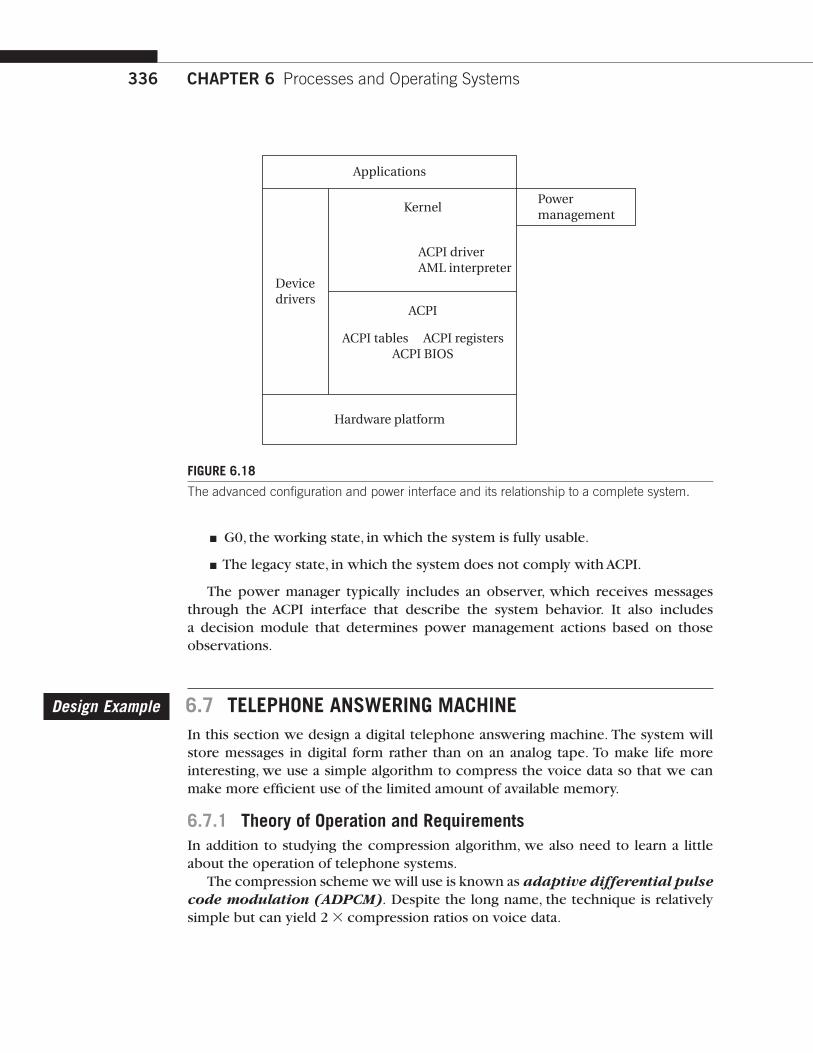
336 CHAPTER 6 Processes and Operating Systems
Applications
Hardware platform
Devicedrivers
Kernel
ACPI driverAML interpreter
ACPI
ACPI BIOS
Powermanagement
ACPI tables ACPI registers
FIGURE 6.18
The advanced configuration and power interface and its relationship to a complete system.
■ G0, the working state, in which the system is fully usable.
■ The legacy state, in which the system does not comply with ACPI.
The power manager typically includes an observer, which receives messagesthrough the ACPI interface that describe the system behavior. It also includesa decision module that determines power management actions based on thoseobservations.
Design Example 6.7 TELEPHONE ANSWERING MACHINEIn this section we design a digital telephone answering machine. The system willstore messages in digital form rather than on an analog tape. To make life moreinteresting, we use a simple algorithm to compress the voice data so that we canmake more efficient use of the limited amount of available memory.
6.7.1 Theory of Operation and RequirementsIn addition to studying the compression algorithm, we also need to learn a littleabout the operation of telephone systems.
The compression scheme we will use is known as adaptive differential pulsecode modulation (ADPCM). Despite the long name, the technique is relativelysimple but can yield 2� compression ratios on voice data.

6.7 Design Example: Telephone Answering Machine 337
Time
Time
Analog signal
ADPCM stream 3 2 1 21 22 23
FIGURE 6.19
The ADPCM coding scheme.
The ADPCM coding scheme is illustrated in Figure 6.19. Unlike traditional sam-pling, in which each sample shows the magnitude of the signal at a particular time,ADPCM encodes changes in the signal. The samples are expressed in a codingalphabet ,whose values are in a relative range that spans both negative and positivevalues. In this case, the value range is {�3,�2,�1, 1, 2, 3}. Each sample is used topredict the value of the signal at the current instant from the previous value.At eachpoint in time, the sample is chosen such that the error between the predicted valueand the actual signal value is minimized.
AnADPCM compression system, including an encoder and decoder, is shown inFigure 6.20. The encoder is more complex, but both the encoder and decoder usean integrator to reconstruct the waveform from the samples. The integrator simplycomputes a running sum of the history of the samples; because the samples aredifferential, integration reconstructs the original signal. The encoder compares theincoming waveform to the predicted waveform (the waveform that will be gen-erated in the decoder). The quantizer encodes this difference as the best predic-tor of the next waveform value. The inverse quantizer allows us to map bit-levelsymbols onto real numerical values; for example, the eight possible codes ina 3-bit code can be mapped onto floating-point numbers. The decoder simplyuses an inverse quantizer and integrator to turn the differential samples into thewaveform.
The answering machine will ultimately be connected to a telephone subscriberline (although for testing purposes we will construct a simulated line).At the otherend of the subscriber line is the central office. All information is carried on thephone line in analog form over a pair of wires. In addition to analog/digital anddigital/analog converters to send and receive voice data, we need to sense twoother characteristics of the line.

338 CHAPTER 6 Processes and Operating Systems
Quantizer
Integrator
IntegratorInversequantizer
Encoder
Decoder
2
Samples
Inversequantizer
FIGURE 6.20
An ADPCM compression system.
■ Ringing: The central office sends a ringing signal to the telephone when acall is waiting.The ringing signal is in fact a 90V RMS sinusoid,but we can useanalog circuitry to produce 0 for no ringing and 1 for ringing.
■ Off-hook: The telephone industry term for answering a call is going off-hook; the technical term for hanging up is going on-hook. (This createssome initial confusion since off-hook means the telephone is active andon-hook means it is not in use, but the terminology starts to make senseafter a few uses.) Our interface will send a digital signal to take thephone line off-hook, which will cause analog circuitry to make the nec-essary connection so that voice data can be sent and received duringthe call.
We can now write the requirements for the answering machine.We will assumethat the interface is not to the actual phone line but to some circuitry that providesvoice samples, off-hook commands, and so on. Such circuitry will let us testour system with a telephone line simulator and then build the analog circuitrynecessary to connect to a real phone line.We will use the term outgoing message(OGM) to refer to the message recorded by the owner of the machine and playedat the start of every phone call.

6.7 Design Example: Telephone Answering Machine 339
Name Digital telephone answering machine
Purpose Telephone answering machine with digital memory,using speech compression.
Inputs Telephone: voice samples, ring indicator.User interface: microphone, play messages button,record OGM button.
Outputs Telephone: voice samples, on-hook/off-hook com-mand. User interface: speaker, # messages indicator,message light.
Functions Default mode:When machine receives ring indicator,it signals off-hook, plays the OGM, and then recordsthe incoming message. Maximum recording length forincoming message is 30 s, at which time the machinehangs up. If the machine runs out of memory, theOGM is played and the machine then hangs up with-out recording.Playback mode:When the play button is depressed,the machine plays all messages. If the play button isdepressed again within five seconds, the messages areplayed again. Messages are erased after playback.OGM editing mode:When the user hits the recordOGM button, the machine records an OGM of up to10 s.When the user holds down the record OGM but-ton and hits the play button, the OGM is played back.
Performance Should be able to record about 30min of total voice,including incoming and OGMs.Voice data are sampledat the standard telephone rate of 8 kHz.
Manufacturing cost Consumer product range: approximately $50.Power Powered byAC through a standard power supply.Physical size and weight Comparable in size and weight to a desk telephone.
We have made a few arbitrary decisions about the user interface in these require-ments. The amount of voice data that can be saved by the machine should in factbe determined by two factors: the price per unit of DRAM at the time at which thedevice goes into manufacturing (since the cost will almost certainly drop from thestart of design to manufacture) and the projected retail price at which the machinemust sell. The protocol when the memory is full is also arbitrary—it would makeat least as much sense to throw out old messages and replace them with new ones,and ideally the user could select which protocol to use. Extra features such as anindicator showing the number of messages or a save messages feature would alsobe nice to have in a real consumer product.

340 CHAPTER 6 Processes and Operating Systems
6.7.2 SpecificationFigure 6.21 shows the class diagram for the answering machine. In addition tothe classes that perform the major functions, we also use classes to describe theincoming and OGMs. As seen below, these classes are related.
The definitions of the physical interface classes are shown in Figure 6.22. Thebuttons and lights simply provide attributes for their input and output values. Thephone line, microphone, and speaker are given behaviors that let us sample theircurrent values.
The message classes are defined in Figure 6.23. Since incoming and OGM typesshare many characteristics,we derive both from a more fundamental message type.
The major operational classes—Controls, Record, and Playback—are definedin Figure 6.24. The Controls class provides an operate( ) behavior that overseesthe user-level operations. The Record and Playback classes provide behaviors thathandle writing and reading sample sequences.
The state diagram for the Controls activate behavior is shown in Figure 6.25.Most of the user activities are relatively straightforward. The most complex is an-swering an incoming call. As with the software modem of Section 5.11,we want tobe sure that a single depression of a button causes the required action to be takenexactly once; this requires edge detection on the button signal.
State diagrams for record-msg and playback-msg are shown in Figure 6.26.Wehave parameterized the specification for record-msg so that it can be used eitherfrom the phone line or from the microphone. This requires parameterizing thesource itself and the termination condition.
Microphone*
Line-in*
Speaker*
Controls
Lights*
Record
Playback
Outgoing-message
Incoming-messageLine-out*
Buttons* 1
1
1
1
1
1
1
1
1 1
11 1
1 1
11
1
**
*
*
FIGURE 6.21
Class diagram for the answering machine.

6.7 Design Example: Telephone Answering Machine 341
Microphone*
sample( )
Line-in*
sample( )ring-indicator( )
Line-out*
sample( )pick-up( )
Speaker*
sample( )
Buttons*
record-OGMplay
Lights*
messagesnum-messages
FIGURE 6.22
Physical class interfaces for the answering machine.
Incoming-message
msg-time
Message
Outgoing-message
length530 seconds
lengthstart-adrsnext-msgsamples
FIGURE 6.23
The message classes for the answering machine.
Controls
operate( )
Playback
playback-msg( )
Record
record-msg( )
FIGURE 6.24
Operational classes for the answering machine.

342 CHAPTER 6 Processes and Operating Systems
Start
Compute button, line activations
Activations?
Play OGM
Play OGM
Play OGM
Record OGM
Record ICM
Play ICM
Play ICM
Wait for time-out
Record OGM Erase
Erasemessages
Erasemessages
Incoming
Allocate ICM
Answer line
End
Time-out
Playactivation
FIGURE 6.25
State diagram for the controls activate behavior.
6.7.3 System ArchitectureThe machine consists of two major subsystems from the user’s point of view: theuser interface and the telephone interface. The user and telephone interfaces bothappear internally as I/O devices on the CPU bus with the main memory serving asthe storage for the messages.
The software splits into the following seven major pieces:
■ The front panel module handles the buttons and lights.
■ The speaker module handles sending data to the user’s speaker.
■ The telephone line module handles off-hook detection and on-hookcommands.
■ The telephone input and output modules handle receiving samples fromand sending samples to the telephone line.

6.7 Design Example: Telephone Answering Machine 343
End
Start
End
Start
tm(voiceperiod)
playback-msgrecord-msg
nextadrs5msg.length
speaker.sample( )5msg.samples[nextadrs]nextadrs11
end(source)
tm(voiceperiod)
F F
T T
msg.samples[nextadrs]5sample(source)
nextadrs50nextadrs50
FIGURE 6.26
State diagrams for the record-msg and playback-msg behaviors.
■ The compression module compresses data and stores it in memory.
■ The decompression module uncompresses data and sends it to the speakermodule.
We can determine the execution model for these modules based on the rates atwhich they must work and the ways in which they communicate.
■ The front panel and telephone line modules must regularly test the buttonsand phone line, but this can be done at a fairly low rate. As seen below, theycan therefore run as polled processes in the software’s main loop.
while (TRUE) {check_phone_line();run_front_panel();
}
■ The speaker and phone input and output modules must run at higher, regularrates and are natural candidates for interrupt processing.These modules don’trun all the time and so can be disabled by the front panel and telephone linemodules when they are not needed.

344 CHAPTER 6 Processes and Operating Systems
■ The compression and decompression modules run at the same rate as thespeaker and telephone I/O modules, but they are not directly connected todevices.We will therefore call them as subroutines to the interrupt modules.
One subtlety is that we must construct a very simple file system for messages,since we have a variable number of messages of variable lengths. Since messagesvary in length, we must record the length of each one. In this simple specifica-tion, because we always play back the messages in the order in which they wererecorded, we don’t have to keep a full-fledged directory. If we allowed users toselectively delete messages and save others, we would have to build some sort ofdirectory structure for the messages.
The hardware architecture is straightforward and illustrated in Figure 6.27. Thespeaker and telephone I/O devices appear as standard A/D and D/A converters.The telephone line appears as a one-bit input device (ring detect) and a one-bit output device (off-hook/on-hook). The compressed data are kept in mainmemory.
6.7.4 Component Design and TestingPerformance analysis is important in this case because we want to ensure thatwe don’t spend so much time compressing that we miss voice samples. In a realconsumer product, we would carefully design the code so that we could use theslowest, cheapest possible CPU that would still perform the required processing inthe available time between samples. In this case,wewill choose the microprocessorin advance for simplicity and simply ensure that all the deadlines are met.
An important class of problems that should be adequately tested is memoryoverflow.The system can run out of memory at any time,not just betweenmessages.The modules should be tested to ensure that they do reasonable things when allthe available memory is used up.
Front panel
A/D
D/A
A/D
D/A
CPU Memory
Mic
Speaker
Telephone line
FIGURE 6.27
The hardware structure of the answering machine.

Summary 345
6.7.5 System Integration and TestingWe can test partial integrations of the software on our host platform. Final testingwith real voice data must wait until the application is moved to the target platform.
Testing your system by connecting it directly to the phone line is not a verygood idea. In the United States, the Federal Communications Commission regulatesequipment connected to phone lines. Beyond legal problems,a bad circuit can dam-age the phone line and incur thewrath of your service provider.The required analogcircuitry also requires some amount of tuning, and you need a second telephoneline to generate phone calls for tests. You can build a telephone line simulator totest the hardware independently of a real telephone line.The phone line simulatorconsists of A/D and D/A converters plus a speaker and microphone for voice data,an LED for off-hook/on-hook indication, and a button for ring generation. The tele-phone line interface can easily be adapted to connect to these components,and forpurposes of testing the answering machine the simulator behaves identically to thereal phone line.
SUMMARYThe process abstraction is forced on us by the need to satisfy complex timingrequirements,particularly for multirate systems.Writing a single program that simul-taneously satisfies deadlines at multiple rates is too difficult because the controlstructure of the program becomes unintelligible.The process encapsulates the stateof a computation, allowing us to easily switch among different computations.
The operating system encapsulates the complex control to coordinate the pro-cess. The scheme used to determine the transfer of control among processes isknown as a scheduling policy. A good scheduling policy is useful across many dif-ferent applications while also providing efficient utilization of the available CPUcycles.
It is difficult,however, to achieve 100% utilization of the CPU for complex appli-cations. Because of variations in data arrivals and computation times, reservingsome cycles to meet worst-case conditions is often necessary. Some schedul-ing policies achieve higher utilizations than others, but often at the cost ofunpredictability—they may not guarantee that all deadlines are met. Knowledge ofthe characteristics of an application can be used to increase CPU utilization whilealso complying with deadlines.
What We Learned
■ A process is a single thread of execution.
■ Pre-emption is the act of changing the CPU’s execution from one process toanother.
■ A scheduling policy is a set of rules that determines the process to run.

346 CHAPTER 6 Processes and Operating Systems
■ Rate-monotonic scheduling (RMS) is a simple but powerful schedulingpolicy.
■ Interprocess communication mechanisms allow data to be passed reliablybetween processes.
■ Scheduling analysis often ignores certain real-world effects. Cache interactionsbetween processes are themost important effects to consider when designinga system.
FURTHER READINGGallmeister [Gal95] provides a thorough and very readable introduction to POSIXin general and its real-time aspects in particular. Liu and Layland [Liu73] introducerate-monotonic scheduling; this paper became the foundation for real-time systemsanalysis and design. The book by Liu [Liu00] provides a detailed analysis of real-time scheduling. Benini et al. [Ben00] provide a good survey of system-level powermanagement techniques. Falik and Intrater [Fal92] describe a custom chip designedto perform answering machine operations.
QUESTIONSQ6-1 Identify activities that operate at different rates in
a. a PDA;
b. a laser printer; and
c. an airplane.
Q6-2 Name an embedded system that requires both periodic and aperiodiccomputation.
Q6-3 An audio system processes samples at a rate of 44.1 kHz. At what ratecould we sample the system’s front panel to both simplify analysis of thesystem schedule and provide adequate response to the user’s front panelrequests?
Q6-4 Draw a UML class diagram for a process in an operating system.The processclass should include the necessary attributes and behaviors required of atypical process.
Q6-5 What factors provide a lower bound on the period at which the system timerinterrupts for preemptive context switching?
Q6-6 What factors provide an upper bound on the period at which the systemtimer interrupts for preemptive context switching?

Questions 347
Q6-7 You are given these periodic tasks:
Task Period Execution time
P1 5ms 2msP2 10ms 3msP3 10ms 3msP4 15ms 6ms
Compute the utilization of this set of tasks.
Q6-8 You are given these periodic tasks:
Task Period Execution time
P1 5ms 1msP2 10ms 2msP3 10ms 2msP4 15ms 3ms
a. Show a cyclostatic schedule for the tasks.
b. Compute the CPU utilization for the system.
Q6-9 For the task set of question Q6-8, show a round robin schedule assumingthat P1 does not execute during its first period and P3 does not executeduring its second period.
Q6-10 What is the distinction between the ready and waiting states of processscheduling?
Q6-11 Provide examples of
a. blocking interprocess communication, and
b. nonblocking interprocess communication.
Q6-12 Assuming that you have a routine called swap(int *a,int *b) that atomicallyswaps the values of the memory locations pointed to a and b, write Ccode for:
a. P( ); and
b. V( ).
Q6-13 Draw UML sequence diagrams of two versions of P( ): one that incorrectlyuses a nonatomic operation to test and set the semaphore location andanother that correctly uses an atomic test-and-set.

348 CHAPTER 6 Processes and Operating Systems
Q6-14 For the following periodic processes,what is the shortest interval we mustexamine to see all combinations of deadlines?
a.Process Deadline
P1 3P2 5P3 15
b.Process Deadline
P1 2P2 3P3 6P4 10
c.Process Deadline
P1 3P2 4P3 5P4 6P5 10
Q6-15 Consider the following system of periodic processes executing on asingle CPU:
Process CPU time Deadline
P1 4 200P2 1 10P3 2 40P4 6 50
Can we add another instance of P1 to the system and still meet all thedeadlines using RMS?
Q6-16 Given the following set of periodic processes running on a single CPU,whatis the maximum execution time for P5 for which all the processes will beschedulable using RMS?

Questions 349
Process CPU time Deadline
P1 1 10P2 18 100P3 2 20P4 5 50P5 x 25
Q6-17 A set of periodic processes is scheduled using RMS. For the process execu-tion times and periods shown below,show the state of the processes at thecritical instant for each of these processes.
a. P1
b. P2
c. P3
Process CPU time Deadline
P1 1 4P2 2 5P3 1 20
Q6-18 For the given periodic process execution times and periods, show howmuch CPU time of higher-priority processes will be required during oneperiod of each of the following processes:
a. P1
b. P2
c. P3
d. P4
Process CPU time Deadline
P1 1 5P2 2 10P3 3 25P4 4 50
Q6-19 For the periodic processes shown below:
a. Schedule the processes using an RMS policy.
b. Schedule the processes using an EDF policy.
In each case, compute the schedule for the hyperperiod of the processes.Time starts at t � 0.

350 CHAPTER 6 Processes and Operating Systems
Process CPU time Deadline
P1 1 3P2 1 4P3 1 12
Q6-20 For the periodic processes shown below:
a. Schedule the processes using an RMS policy.
b. Schedule the processes using an EDF policy.
In each case,compute the schedule for an interval equal to the hyperperiodof the processes. Time starts at t � 0.
Process CPU time Deadline
P1 1 3P2 1 4P3 2 8
Q6-21 For the given set of periodic processes,all of which share the same deadlineof 12:
a. Schedule the processes for the given arrival times using standard rate-monotonic scheduling (no data dependencies).
b. Schedule the processes taking advantage of the data dependencies. Byhow much is the CPU utilization reduced?
P3P2
P1
Process CPU time
P1 2P2 1P3 2

Questions 351
Q6-22 For the periodic processes given below,find a valid schedule
a. using standard RMS, and
b. adding one unit of overhead for each context switch.
Process CPU time Deadline
P1 2 30P2 4 40P3 7 120P4 5 60P5 1 15
Q6-23 For the periodic processes and deadlines given below:
a. Schedule the processes using RMS.
b. Schedule using EDF and compare the number of context switchesrequired for EDF and RMS.
Process CPU time Deadline
P1 1 5P2 1 10P3 2 20P4 9 50P5 7 100
Q6-24 In each circumstance below, would shared memory or message passingcommunication be better? Explain.
a. A cascaded set of digital filters.
b. A digital video decoder and a process that overlays user menus on thedisplay.
c. A software modem process and a printing process in a fax machine.
Q6-25 If you wanted to reduce the cache conflicts between the most computa-tionally intensive parts of two processes,what are two ways that you couldcontrol the locations of the processes’ cache footprints?
Q6-26 Draw a state diagram for the predictive shutdown mechanism of a cellphone. The cell phone wakes itself up once every five minutes for 0.01second to listen for its address. It goes back to sleep if it does not hear itsaddress or after it has received its message.
Q6-27 Howwould you use theADPCMmethod to encode an unvarying (DC) signalwith the coding alphabet {�3,�2,�1, 1, 2, 3}?

352 CHAPTER 6 Processes and Operating Systems
LAB EXERCISESL6-1 Using your favorite operating system, write code to spawn a process that
writes “Hello, world” to the screen or flashes an LED, depending on youravailable output devices.
L6-2 Build a small serial port device that lights LEDs based on the last characterwritten to the serial port. Create a process that will light LEDs based onkeyboard input.
L6-3 Write a driver for an I/O device.
L6-4 Write context switch code for your favorite CPU.
L6-5 Measure context switching overhead on an operating system.
L6-6 Using a CPU that runs an operating system that uses RMS, try to get the CPUutilization up to 100%.Vary the data arrival times to test the robustness of thesystem.
L6-7 Using a CPU that runs an operating system that uses EDF, try to get the CPUutilization as close to 100% as possible without failing. Try a variety of dataarrival times to determine how sensitive your process set is to environmentalvariations.