191

Chapter 5

Particles and Particle Technology

Solids appear in one of two forms, either as crystals or powders. The

difference is one of size, since many of the powders we use are in reality very

fine crystals. This, of course, depends upon the manne r in which the solid is

prepared. Nevertheless, mos t solids that we encounter in the real world are

in the form of powders. That is, they are in the form of discrete small

particles of varying size. Each particle has its own unique diameter and size.

Additionally, their physical propor t ions can vary in shape from spheres to

needles. For a given powder, all grains will be the same shape, but the

particle shape and size can be altered by the me thod used to create them in

the first place. Methods of part icle formation include:

Precipi ta t ion

Solid state reac t ion

Condensat ion

In this Chapter, we in tend to investigate mechan i sms of particle growth. We

wiU, in the next chapter , address the me thods used to form (grow) single

crystals and how they have been utilized. Certain proper t ies of part icles ,

including m e a s u r e m e n t of size, will be discussed later in this chapter. But

first, we need to define exactly what we mean by a part icle.

In the previous chapter , we covered mechan i sms relating to solid state

reactions, formation of nuclei and the rate of their growth in both

he terogeneous and homogeneous solids. Still other processes exist after particles have formed, including sequences in particle growth. We have

already ment ioned p rec ip i t a t ioa as one m e t h o d for obtaining d i sc re te

particles. As indicated in the previous chapter , nucleat ion in prec ip i ta t ion

processes can be homogeneous (no outside influences) or he terogeneous (by

specific outside coercion). In precipi tat ion processes to form a dis t r ibut ion

of particle sizes, it is probably a combinat ion of both mechan i sms .

192

5 . 1 . - SEQUENCES IN PARTICLE GROWTH

We have already shown that embryo formation leads to nucleat ion, and that

this nucleat ion preceeds any solid state reaction or change of state. In a like

manner , nuclei m u s t form in order for any precipi tat ion process to p roceed .

Once formed, these nuclei then grow until impingement of the growing

particles occurs. Impingement implies that all of the nu t r ien t supplying the

particle growth has been used up. This m echan i sm applies to both solid state

reaction and precipi tat ion processes to form product particles. Then a

process known as O~wald R i l~n lng takes over. This process occurs even at

room tempera ture . The sequences in particle growth are:

5.1.1.- Embryo format ion

Nucleat ion

Nuclei Growth

I m p i n g e m e n t

Ostwald Ripening (coarsening)

S in te r ing

Formation of Grain Boundaries

We have already covered the first three in some detail. Impingement involves

the point where the growing particles actually touch each other and have

used up all of the nu t r ien t which had originally caused them to s tar t growing.

Ostwald r ipen ing usually occurs between particles, following i m p i n g e m e n t ,

wherein larger particles grow at the expense of the smaller ones. One

example of this would be if one had a precipi tate already formed in solution.

In many cases, the smaller part icles redissolve and reprecipi ta te on the

larger ones, causing them to grow larger. Interfacial tension between the

particles is the driving force, and it is the surface area that becomes

minimized. Thus, larger particles, having a total lower surface area, increase

at the expense of numerous smaller particles which have a relatively high

surface area.

193

Ostwald r ipening differs from nuclei growth in tha t the relative size and

numbers of part icles change, whereas in nuclei growth, the number s of

particles growing from nuclei do not change. Sintering, on the other hand, is

an entirely different process, and usually occurs when external heat is

applied to the part icles .

5.2. - SINTERING, SINTERING PROCESSES AND GRAIN GROWTH

Sinter ing of particles occurs when one heats a sys tem of particles to an

elevated tempera ture . It is caused by an interact ion of particle surfaces

whereby the surfaces fuse together and form a solid m a s s . It is related to a

solid state reaction in that s inter ing is governed by diffusion processes, but

no solid ~cat~ react ion, or change of composi t ion or state, takes place. The

best way to i l lustrate this p h e n o m e n o n is to use pore growth as an example.

When a sys tem of particles, i.e.- a powder, is heated to high t empera tu re ,

the particles do not undergo solid state reaction, unless there is more than

one composi t ion present . Instead, the part icles tha t are touching each o the r

will sinter, or fuse together , to form o n e larger particle. Such a m e c h a n i s m

is i l lustrated in the following diagram, given as 5.2.1. on the next page.

As can be seen, voids arise when the particles fuse together. The void space

will depend upon the original shape of the particles. In 5.2.1., we have

shown spherical part icles which produce only a few voids. Additionally, an

overall change in the total volume of the particles, and that of the fusion

product , occurs. Mostly, the change is negative, but in a few cases, it is

positive. Experimentally, this change is a very difficult problem to measure .

What has been done is to form a long thin bar or rod by put t ing the p o w d e r

into a long thin mold and press ing it in a hydraulic press at many tons pe r

square inch. One can then measure the change of volume induced by

sintering, by measur ing a change in length as related to the overall length of

the rod.

194

It has been found tha t the s in te r ing of m a n y ma te r i a l s can be re la ted to a

power law, and tha t the ~arlxflmge, AL, can be desc r ibed by:

5.2.2.- AL /Lo = k t m

where k is a cons tan t , Lo is the original length, t is the t ime of s in ter ing, and

the exponent , m , is d e p e n d e n t upon the mate r i a l be ing invest igated. It has

also been fu r the r d e m o n s t r a t e d tha t a cons iderab le difference exis ts b e t w e e n

the s in te r ing of Rne and coarse par t ic les , as shown in the following d iagram,

given as 5.2.3. on the next page.

In this case, the "fine" par t ic les and the "coarse" par t ic les were s e p a r a t e d so

tha t the difference in size be tween individual par t ic les was min imized . T h a t

is, m o s t of the individual par t ic les in each fract ion were a lmos t the s a m e

size. Both the fine and coarse par t ic les have a s in te r ing slope of 1 /2 bu t it is

the coarse par t ic les wh ich s in te r to form a solid having a dens i ty c loses t to

195

theoretical density. This is an excellent exaumple of the effect of pore volume,

or void formation, and its effect upon the final density of a solid formed by

powder compact ion and s inter ing techniques. Quite obviously, the fine

particles give rise to many more voids than the coarser particles so that the

at tained density of the final s intered solid is m u c h less than for the solid

prepared using coarser particles. It is also clear that ff one wishes to obtain a

s intered product with a density close to the theoret ical density, one needs to

s tar t with a particle size distr ibution having particles of varied diameters so

that void volume is min imized .

The next subject we will discuss is that of grain growth. The s implest way to

i l lustrate this factor is th rough the s inter ing behavior of aggregates. An

aggregate is defined a large particle, composed of many small particles, as

shown in the following diagram, given as 5.2.4. on the next page.

In this diagram, two steps are implicit. It is the aggregates, composed of

very fine specks, which sinter to form larger grains (particles).

196

But, since many part icles are growing at the same time, growth occurs until

impingement . The formation of boundar ies between the part icles (grains)

growing thus results. It is these grains which form the final s in tered whole.

Note that the crystallographic orientat ion of each grain differs from that of

its neighbors, as i l lustrated in the above diagram.

When a system of very fine part icles is formed, the interfacial tension is high

due to the very high surface area present . Agglomerates (weak surface energy

interchange) will form, or a4 j [~~ates (strong surface energy in te rchange)

can result, especially ff the Ostwald r ipening m e c h a n i s m is slow, or is

inhibited. Immediate removal of a precipi tate from its "mother liquor" is one

example where the likelihood of aggregate formation is enhanced. S in te r ing

then produces both pore growth and grain growth. This m e c h a n i s m also

applies to powder compact ion processes where aggregates may be p resen t in

the powder. Sintering then leads to grain growth as well.

It should be clear, then, that the precipi tat ion process needs to be

controlled carefully in order to produce a mater ia l composed of part icles of a

desired configuration. Both Ostwald riping and sinter ing can be utilized to

obtain a particle of desired size, d imensions and particle habit. Industr ia l

technologists have taken advantage of these particle forming and al ter ing

197

mechanisms . One example of this type of particle growth is descr ibed as

follows.

In f luorescent lamps, a layer of phosphors is applied to the inside of a glass

tube by means of a suspens ion of particles, i.e.- the ha lophosphate p h o s p h o r Sb ~+ Mn 2+ (plus minor amounts of having a composit ion of: (MsF, CI(PO4)s:

other phosphors to achieve certain "colors"). It has been de te rmined that

the lamp br ightness and durat ion of light output (maintenance) is highly

dependan t upon how well the the internal surface of the glass is covered by

the particles. By mainta in ing precipi tat ion condit ions so tha t small th in

squares of CaHP04 result from the precipi ta t ing solution, a m a x i m u m

coverage of the glass is achieved. Precipitat ion occurs by adding a solution of

(NH4)2HP04 to a solution of CaCI~. The resul t ing precipi ta te is consists of very

fine part icles and is not very crystalline. As a ma t t e r of fact, the par t ic les

were usually ill-defined and bordered upon amorphous . The solution

t empera tu re is then raised so that Ostwald r ipening can occur. As the larger

crystaUites begin to grow, the smaller i l l -defined crystallites, having a m u c h

larger surface area, dissolve and reprecipi ta te upon the larger ones. The

resul t ing single-crystal squares, i.e.- El, have an average size of about 25~m.

The solid state react ion to form the ha lophosphate phosphor is:

5.2.5.- 6 CaHPO 4 + 3 CaCY)~ + ~ 2 ~ 2 C~ F (P04) a

where we have not shown the Sb20~ and MnCOs added as "activators". The

ha lophosphate thus produced follows the crystal habit of the major

ingredient , in this case that of CaHP04 habit. When applied, the thin squares

lie fiat and overlap on the glass surface. During s inter ing at about 1200 ~

the CaHP04 does not dis integrate but undergoes an internal r e a r r a n g e m e n t

to form (M~207 while mainta in ing the same crystal habit. The CaCX) 3

dis integrates into small part icles (like BaCOn) while CaF2 exhibits a

sublimation pressure at the firing tempera ture . The resul t ing solid s tate

reaction to form the ha lophosphate product thus depends upon the crystal

habit of the major ingredient , CaHPO4.

198

The same type of mechan i sms apply to other materials. Even where a meta l

is mel ted and then cast, nucleat ion leads to formation of many fine par t ic les

in the sub-solidus (partially solidified) state. This leads to grain growth in the

solid metal, thereby lowering its s t rength. Sometimes, special additives are

added to the melt to slow nucleat ion during cooling, thereby increasing the

s t rength of the metal product .

Another example is our old friend, BaC03. If we fire this solid compound in

air at a very high t empera tu re for a long time, we get several changes. First,

it decomposes to very free particles of BaO. These fine particles have a large

surface area, and with cont inued ruing sinters to form larger part icles .

Eventually, the particles get big enough, and the porosity decreases to the

point where grain boundar ies begin to form between particles. The grains

sinter together to form a large particle with many grain boundaries . It should

be again be emphasized that each grain in the large particle is essentially a

small single crystal with its lattice oriented in a slightly different d i rec t ion

from that of it neighbors (see 5.2.4.) .

Let us now consider the the rmodynamics of sintering. There are two types of

s intering which are d is t inguished by the change in volume which occurs.

These are:

5.2.6.- NO SHRINKAGE : dV/dt = 0

WITH SHRINKAGE : dV/dt = f(V)

As we have already said, the change in volume, from initial state to final state,

can be positive or negative, but is usually negative. The driving force is a

decrease in Gibbs free energy, AG. It is related to both the interfacial tens ion

(surface energy), V, and the surface energy of the particles (which is re la ted

to their size), viz-

5.2.7.- d G = y dA

199

Cons ide r a m o r e fami l iar example , t h a t of a d rop le t s i t t ing u p o n the sur face

of a l iquid . The d rop le t ha s a rad ius , r, a n d t h e r e are n - m o l e s of l iquid w i t h i n

it wi th a mola l vo lume, V. To fo rm the d rop le t r e q u i r e s an a m o u n t , nV, of t h e

l iquid, w h e r e V is the f rac t iona l m o l a r vo lume of the drople t . Th is gives us:

5 .2 .8 . - nV = 4 / 3 n r 3

a n d the c h a n g e in free ene rgy to fo rm the d rop le t is:

5 .2 .9 . - dG = A G d n = y dA

If we now d i f fe ren t ia te t h e s e equa t ions , i .e.-

5 . 2 . 1 0 . -

and:

Volume of Droplet : n = 4n r 3 / 3 V so that : (In = 4n /V r 2 d r

Sur face Area of Droplet : A = 4n r 2 so that : dA = 8n r d r

we can p u t all of the e q u a t i o n s t o g e t h e r so as to yield the Kelvin equa t ion for

c h a n g e in free ene rgy as a func t ion of the r a d i u s of the s p h e r i c a l pa r t i c l e :

5 . 2 . 1 1 . - AG = 2 y V / r

One c a n do the s a m e for a cubic par t ic le , in fact for any s h a p e factor. S i n c e

the c h e m i c a l po ten t ia l , p , is r e l a t e d to AG, we use the following equa t ions :

5 . 2 . 1 2 . - -Po = A G = R T l n p / p o

2 y V / r = R T I n p / p o

or: p = p o exp (2 y V / r R T )

If we now define ~p = p - Po , t h e n :

2 0 0

5 . 2 . 1 3 . - P /Po = 1 + Ap/po

Mathemat i ca l ly , In (I + Ap / Po ) -= AP / Po (within 5% ff ~p / Po

we get the a p p r o x i m a t e equa t ion :

5 . 2 . 1 4 . - Ap/po = 2 y V / r - I / R T

>_ 0 . I ) . T h u s

It i s t h i s e q u a t i o n w h i c h h a s b e e n u s e d m o r e than any o t h e r to

s i n t e r i n g . To evaluate i ts use , c o n s i d e r the following e x a m p l e .

A l u m i n a , A1203, is a very r e f r ac to ry c o m p o u n d . It m e l t s above 1950 ~ and

is not very reac t ive w h e n hea t ed . If we a t t e m p t to s in t e r it a t 1730~ w e

f'md the following values to apply:

5 . 2 . 1 5 . - ~ P / P o =- 0. I

y -= 2000 dyne / cm.

V = M / d = 25 .4 c c . / m o l

R = 8.3 x 10 -7 e r g / m o l

r = 6 x 10 - 6 c m = 0 . 0 6 m i c r o n

Wha t th i s m e a n s is t h a t ff the a l u m i n a pa r t i c l e s are s m a l l e r t h a n about 0 . 0 6

mic ron , t hey will n o t s inter . Even t h o u g h the above is an a p p r o x i m a t i o n , t h e

specif ic case for a l u m i n a has b e e n c o n f i r m e d e x p e r i m e n t a l l y .

THUS, WE HAVE SHOWN THAT IF THE PARTICLES ARE TOO SMALL, THEY

WILL NOT SINTER. NORMAL NUCLEI GROW22-1 THROUGH DIFFUSION

PROCESSES REMAINS THE NORM UNTIL THE PARTICLES GET LARGE

ENOUGH TO SINTER.

Let us now e x a m i n e w h y th is m e c h a n i s m m i g h t be t rue . In the case of

s i n t e r i ng of sphe re s , we can define two ca se s as before, t h a t of no s h r i n k a g e

a n d t h a t of sh r i nkage , bo th as a func t ion of vo lume. If we have two s p h e r e s in

201

direct contact , we can define cer ta in p a r a m e t e r s , as shown in the following

diagram:

We s ta r t wi th s p h e r e s of radius , r, in direct contact . The two cases shown

are:

1) n o ~ll- lnkage

2} w i th sh r inkage ,

Actual s in te r ing occurs by flow of m a s s from each sphe re to the mu tua l po in t

of contact , which gradual ly th ickens . We cmn es t imate the volume of mass , V,

at the con tac t area, A, in t e r m s of the foUov~mg pa rame te r s : r, the rad ius of

the spheres ; p , the t h i c k n e s s of the layer bui ldup; and x, the rad ius of

contac t of the bui l t -up layer. If we have shr inkage , t hen we m u s t also evaluate

h, the a m o u n t of shr inkage , shown above as the he ight of in te r l ink ing layer.

This model br ings us to an i m p o r t a n t point, vis: If the s p h e r e s are too small ,

the re can be little m a s s flow to the area of joining (sintering) of the s p h e r e s .

Actually, it is the ra te of flow of m a s s to the joining a rea tha t is i m p o r t a n t and

the a rea of touch ing of the s p h e r e s vail d e t e r m i n e this .

2 0 2

It is therefore logical that a s ize l i m i ~ should apply to the case of

s i n t e r i n g a n d its m e c h a n i s m s . If the sphe res are too small, t hen there is no t

enough touching area and volume for the s in ter ing m e c h a n i s m to occur .

The actual values of the s in ter ing pa r ame te r s have been found to be:

5 .2 .17 . -

VALUES OF SINTERING PARAMETERS

V h A

No Sh r inkage nx21 2 r 0 n2x21r

,

With Sh r inkage nx 2 / 2r x2 / 2r n2x3 / 2r

x 2 / 2 r

x 2 / 4r

M o s t sys tems exhibit sh r inkage in s in ter ing and it has been found tha t t he

following equat ion applies:

5 .2 .18 . - AL /Lo = h / r a n d x = c t m

where t is the t ime of s inter ing, h is a charac ter i s t ic s in ter ing cons t an t for

shr inkage , and m is an exponen t d e p e n d e n t upon the m e c h a n i s m of

s in te r ing .

We have indica ted tha t flow of mas s is impor t an t in s inter ing. There are

several operat ive m e c h a n i s m s which are de t e rmined by the type of mate r i a l

involved. Actually, the s tudy of s in ter ing deserves a separa te chapter , bu t we

will only summar ize the major m e c h a n i s m s tha t have been observed for the

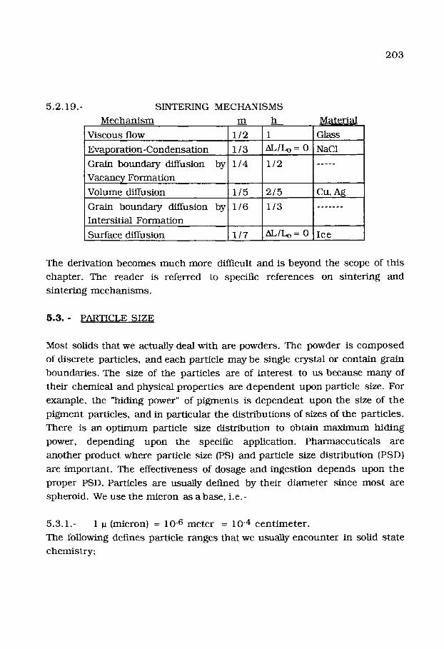
cons tan t s of 5.2.18. These are given in 5.2.19. on the next page.

Note tha t the values of h depends upon the mater ia l and the m e c h a n i s m of

s intering. Also, these values depend upon r and x, the radii of the pa r t i c les

and the radius of joining. These equat ions apply only to sphero ids and a

shape factor m u s t be cons ide red as well .

203

5 .2 .19. - SINTERING MECHANISMS

Mechan i sm

Viscous flow . . . . . .

Evaporat ion-Condensat ion

Grain boundary diffusion

Vacancy Format ion

Volume diffusion

m

1/2

1/3

by ~/4

h

1

~./~ = o . . . . .

1/2

1/5 2 /5 . . . . .

Grain boundary diffusion by 1/6 1/3

Intersit ial Format ion . . . . .

Surface diffusion 1/7 5L/Lo = 0

Material

Glass

NaCI

Cu, Ag

Ice

The derivation becomes much more difficult and is beyond the scope of this

chapter . The reader is referred to specific references on s inter ing and

sinter ing mechan i sms .

5 . 3 . - PARTICLE SIZE

Most solids tha t we actually deal with are powders. The powder is c o m p o s e d

of discrete particles, and each particle may be single crystal or contain grain

boundaries . The size of the part icles are of interest to us because many of

their chemical and physical proper t ies are dependen t upon particle size. For

example, the "hiding power" of p igments is dependen t upon the size of the

p igment particles, and in part icular the dis tr ibut ions of sizes of the part icles .

There is an op t imum particle size distr ibution to obtain m a x i m u m hid ing

power, depending upon the specific application. Pharmaceut ica ls are

another product where particle size (PS) and particle size distr ibution (PSD)

are important . The effectiveness of dosage and ingest ion depends upon the

proper PSD. Particles are usually defined by their d iameter since most are

spheroid. We use the micron as a base, i.e.-

5.3.1.- 1 ~ (micron) = 10 -6 meter = 10 "4 cen t ime te r .

The following defines particle ranges that we usually encounter in solid state

chemis t ry :

2 0 4

5 .3 .2 . -

PARTICLE RANGES

Range .Centime.ter .s ~ D e s c r i p t i o n

Macro 1.0 - 0 . 0 5 104 - 5 0 0 Gravel

Mic ro 0 .01- 0 . 0 0 0 1 I 0 0 - 1.0 "Normal"

S u b - m i c r o 0 . 0 0 0 1 - 10 -7 1.0 - 0 . 0 0 1 Colloidal

It is eas ie r to desc r ibe PS in t e r m s

c e n t i m e t e r s .

of m i c r o n s r a t h e r t h a n m e t e r s o r

In the real world, we e n c o u n t e r pa r t i c l e s in a var ie ty of forms, a l t h o u g h w e

m a y not recognize t h e m as such . In the following d i ag ram, given as 5 .3 .3 . on

the nex t page , are s u m m a r i z e d m a n y of the pa r t i c l e s of in t e re s t . At the top of

the d iag ram, the pa r t i c l e d i a m e t e r s in m i c r o n s is shown. I m m e d i a t e l y be low

are s t a n d a r d s c r e e n sizes, i nc lud ing bo th U. S. a n d Tyler s t a n d a r d m e s h .

S c r e e n s are m a d e by t ak ing a m e t a l wire of specific d i a m e t e r a n d c ros s -

weav ing it to form a s c r e e n wi th specific ho le sizes in it. Thus , a 4 0 0 m e s h

s c r e e n will pas s 37~ pa r t i c l e s or smal le r , b u t hold up all t hose w h i c h a re

larger . A 60 m e s h s c r e e n will pa s s up to 250~ par t i c les , etc. (U. S. S c r e e n

Mesh) .

This d i a g r a m p laces a n d def ines the size of m o s t of the pa r t i c l e s t h a t we are

l ikely to e n c o u n t e r in the real world. On the left is a c o m p a r i s o n of

a n g s t r o m s (/~) a n d m i c r o n s up to 1 ~ = 10, 000 A . In the m i d d l e of t h e

sec t ion , "Equiva lent S i z e s " , is a c o m p a r i s o n of sizes a n d " theore t i ca l m e s h " .

Why the l a t t e r t e r m is s o m e t i m e s u s e d will be d i s c u s s e d later . In " T e c h n i c a l

Defini t ions", size r a n g e s are given for var ious types of sol ids in gases , l iqu ids

in gases , a n d those for soft. In addi t ion , we have a s e p a r a t e c lass i f ica t ion for

w a t e r in air (fog). Finally, t h e r e is a c lass i f ica t ion for var ious c o m m e r c i a l

p r o d u c t s a n d b y - p r o d u c t s we m i g h t e n c o u n t e r , i nc lud ing v i ruses and

bac te r ia . Note the var ied sizes of pa r t i c l e s t h a t we n o r m a l l y e n c o u n t e r . T h i s

l i s t ing is no t m e a n t to be all- inc lus ive bu t ou t l ines m a n y a reas of t e c h n i c a l

i n t e r e s t w h e r e the sizes of pa r t i c l e s are i m p o r t a n t .

205

2 0 6

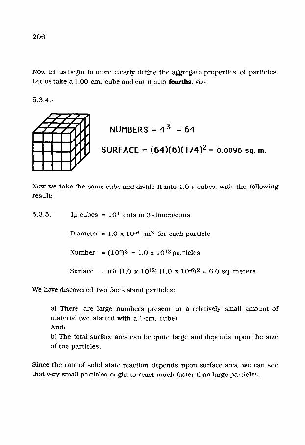
Now let us begin to m o r e clearly define the aggregate p r o p e r t i e s of pa r t i c l e s .

Let us take a 1.00 cm. cube and cu t it into four ths , viz-

5 .3 .4 . -

mmmmele mUll(), mmmm

NUMBERS - 43 _ 64

SURFACE = (64)(6 )( I/4 )2 = 0.0096 sq. m.

Now we take the s a m e cube a n d divide it into 1.0 ~ cubes , wi th the fol lowing

resul t :

5 .3 .5 . - I~ cubes = 10 4 cu t s in 3 - d i m e n s i o n s

Diamete r = 1.0 x i 0 -6 m 3 for each pa r t i c l e

N u m b e r = ( 104) 3 = 1.0 x 1012 p a r t i c l e s

Surface = (6) (1.0 x 1012) (1.0 x 10-6) 2 - 6 .0 sq. m e t e r s

We have d i scovered two facts about pa r t i c l e s :

a) There are large n u m b e r s p r e s e n t in a relat ively smal l a m o u n t of

ma te r i a l (we s t a r t ed wi th a 1-cm. cube) .

And:

b) The total sur face a rea can be qui te large and d e p e n d s u p o n the size

of the pa r t i c l e s .

Since the ra te of solid s ta te r eac t ion d e p e n d s u p o n sur face area, we can see

t ha t very smal l par t ic les ough t to r eac t m u c h fas ter t h a n large pa r t i c l e s .

207

Another observat ion is t ha t solid s ta te reac t ions involving very fine pa r t i c l e s

ought to be very fast in the beginning , bu t t hen will slow down as the p r o d u c t

par t ic les become larger. There are o ther p rope r t i e s of par t ic les which we

can th ink of, as follows:

5.3.6.- PROPERTIES OF PARTICLES

Size Surface area Poros i ty Aggrega tes

Shape Densi ty Pore size N u m b e r s

Agg lomera t e s

Size d i s t r ibu t ion

At this point, we are m o s t i n t e r e s t e d in the size of par t ic les and how t h e

o ther factors re la te to the ques t ion of size. The next m o s t i m p o r t a n t factor is

shape . Most of the par t ic les tha t we will e n c o u n t e r are sphe ro ida l or oblong

in shape, bu t ff we discover tha t we have needle- l ike (acicular) par t ic les , how

do we define the i r average d i ame te r? Is it an average of the s u m of l eng th

plus c ross-sec t ion , or w h a t ?

5 . 4 . - PAR~CLE DISTRIBUTIONS

F u n d a m e n t a l to par t ic le technology is the factor ,s /ze distribution. By this, we

m e a n the n u m b e r of e a c h size in a given collect ion of par t ic les . F rom a c lose

examina t ion of 5.3.3. , it is evident tha t we m u s t deal wi th large n u m b e r s of

par t ic les , even w h e n we have a smal l s t a r t i ng sample weight . This p r o b l e m

becomes c learer ff we corre la te n u m b e r s of par t ic les wi th size, s t a r t ing w i t h

a cube, one (1) cm in size, as in 5.3.4. , and m a k e the cu ts ind ica ted in

5.4.1, given on the next page.

Having done so, we mix the seven (7) sepa ra te p roduc ts . We could then p lo t

the par t ic le d is t r ibut ion as shown in 5.4.2. , also given on the nex t page,

where we have p lo t ted the log of the size of par t ic les in mic rons vs: the log

of the n u m b e r of par t ic les c rea ted . Obviously, the re is a l inear r e l a t i onsh ip

be tween the two variables. The o the r factor to note is tha t this d i s t r ibu t ion

cons is t s of specific (discrete) sizes of par t ic les .

2 0 8

5 .4 .1 . - Var ious Sized Cuts of a One C e n t i m e t e r Cube

Size N u m b e r / c m 3

1 ~ 1.0 x 1012

I0 ~ 1.0 x 109

50 / J 8.3 x 106

1 0 0 ~ 1 .0 x 1 0 6

250 la 6 .4 x 104

500 ~ 8.3 x 103

1000 ~ 1.0 x 103

5 .4 .2 . - A DISCRETE P O P U I ~ T I O N OF PARTICLES

to

L. 12

E c 13

0

~ 4 0

0 1 2 3

log p

In Nature , however , we always have a c o n t i n u o u s d i s t r i bu t ion of p a r t i c l e s .

This m e a n s t ha t we have all sizes, even those of f rac t iona l p a r e n t a g e , i .e .-

18.56V, 18.57V, 18.58 ~, etc. ( suppos ing t h a t we can m e a s u r e 0 .01

dif ferences) . The r e a s o n for th i s is t h a t the m e c h a n i s m s for p a r t i c l e

fo rmat ion , i.e.- p r ec ip i t a t i on , embryo a n d n u c l e a t i o n growth , Os twald

r ipen ing , a n d s in te r ing , are rm~_d_c~n p r o c e s s e s . Thus , whi le we m a y s p e a k of

the "s ta t i s t ica l var ia t ion of d i ame te r s " , a n d whi le we u se w h o l e n u m b e r s for

the par t i c le d i a m e t e r s , the ac tua l i ty is t h a t the d i a m e t e r s are f rac t ional in

n a t u r e . Very few *par t i c le - s ize" spec ia l i s t s s e e m to recognize th i s fact. S i n c e

the p r o c e s s e s are r a n d o m in n a t u r e , we can use s t a t i s t i c s to desc r ibe t h e

2 0 9

p r o p e r t i e s of a popu la t i on of pa r t i c les , a n d the pa r t i c l e size d i s t r ibu t ion .

S ta t i s t i ca l ca lcu la t ion is well su i t ed for th i s p u r p o s e s ince it w a s or ig ina l ly

d e s i g n e d to h a n d l e large n u m b e r s in a popu la t ion . It s h o u l d be c lear t h a t w e

do have a popu l a t i on of pa r t i c l e s in any given pa r t i c l e d i s t r i bu t ion .

5 .5 , - PARTICLE DISTRIBUTIONS AND THE BINOMIAL T H E O R E M

To desc r ibe par t i c le d i s t r ibu t ions , we will u se ou r own n o m e n c l a t u r e , bu t

will soon find t h a t it is r e l a t ed to the sc i ence of s t a t i s t i c s as well. We b e g i n

by the u se of the Probabi l i ty Law.

If we are given n - t h i n g s w h e r e we choose x var iables , t a k e n r at a t ime, t h e

ind iv idua l p robab i l i ty of choos ing (1 + x) will be:

5 .5 .1 . - Pi = (I + x ) n

This is the BINOMIAL THEOREM. Using a Taylor Expans ion , we can find t h e

to ta l p robabi l i ty for i t e m s t a k e n r a t a t ime as:

5 .5 .2 . - P(r) = I n } pr (I - p ) n - r

w h e r e -

5 .5 .3 . { n~ ---- { r}

nCr = n ! / r ! ( n - r ) !

If we now let n a p p r o a c h infinity, t h e n we get-

5 .5 .4 . - P(r) = E Pi = I / [ 2n n p ( I -p)] I/2 . exp (- x 2 / 2np ( I -p)

One will i m m e d i a t e l y recognize th i s as a fo rm of the BOLTZMANN equa t ion ,

or the GAUSSIAN LAW. We can modi fy th i s equa t i on a n d p u t it in to a f o r m

m o r e su i tab le for ou r u s e by m a k i n g the following de f in i t ions .

2 1 0

m

Firs t , we def ine a m e a n (average) s ize of p a r t i c l e s in t he d i s t r i b u t i o n as d ,

a n d t h e n def ine w h a t we call a " s t a n d a r d devia t ion" as o, for t he d i s t r i b u t i o n

of pa r t i c l e s . F r o m s t a t i s t i c s , we k n o w t h a t th i s m e a n s t h a t 6 8 % of t h e

p a r t i c l e s a re b e i n g c o u n t e d (34% on e i t h e r s ide of the m e a n , d), i.e. -

m

5 . 5 . 5 . - Z ( d + d o ) = 0 . 6 8

w h e r e do is t h e d i a m e t e r m e a s u r e d to give + 34% of the to ta l n u m b e r of

pa r t i c l e s . In a l i k e m a n n e r :

m

5 . 5 . 6 . - 2 o ---- 0 . 9 5 4 = Z ( d • d2o )

3 o ----_ 0 . 9 9 9 = Z ( d + d 3 o )

Note t h a t t h e s e s t a n d a r d dev i a t i ons only app ly if we have a Gauss i an

d i s t r i bu t i on . In th i s way, we c a n spec i fy w h a t f r ac t ion we have of t h e to ta l

d i s t r i bu t i on , or loca te p o i n t s in t he d i s t r i bu t i on . By f u r t h e r de f in ing :

5 . 5 . 7 . - m

n p i ~- fl

o ---- ( np ( 1 - p ) 1/2 = s td . dev.

r ~ n p + x = d + x = ( d - d )

we c a n o b t a i n e x p r e s s i o n s to d e s c r i b e a pa r t i c l e d i s t r i b u t i o n w h e r e we have

u s e d x as a dev ia t ion f r o m the m e a n .

Th i s t h e n b r i n g s us to t he e x p r e s s i o n for t he GAUSSIAN PARTICLE S I Z E

DISTRIBUTION, as s h o w n in t he fo l lowing:

5 . 5 . 8 . - m

Pr = 1 exp ( - [ d - d ]2)

(2n) II2 o 2 02

if: { _ o o < d < + o o }

Let us n o w e x a m i n e a G a u s s i a n d i s t r i b u t i o n . A plot is s h o w n as fol lows:

211

What we have is the familiar "Bell-Shaped" curve. This d is t r ibut ion has b e e n

variously called:

5 .5 .10 . -

Gaussian

Log Normal

Bol tzmann

Maxwell - Bol tzmann

We shall use the t e rm "Log Normal" for r easons which will clear later. It

should be now appa ren t tha t we use t e rms bor rowed from stat is t ics and a

stat is t ical approach to descr ibe a d is t r ibut ion of part icles. The two

discipl ines are well sui ted to each o ther since s ta t is t ics is easily capable of

handl ing large assemblages , and the solid s ta te p rocess with vchich we deal

are r a n d o m growth p rocesses which p roduce large n u m b e r s of par t ic les .

Let us now give some examples of the log-normal dis tr ibut ion. A

r ep re sen t a t i on of several types of these d is t r ibut ions is given on the n e x t

page as 5 .5 .11 .

In this diagram, the p a r a m e t e r s of the various log normal d is t r ibut ions are

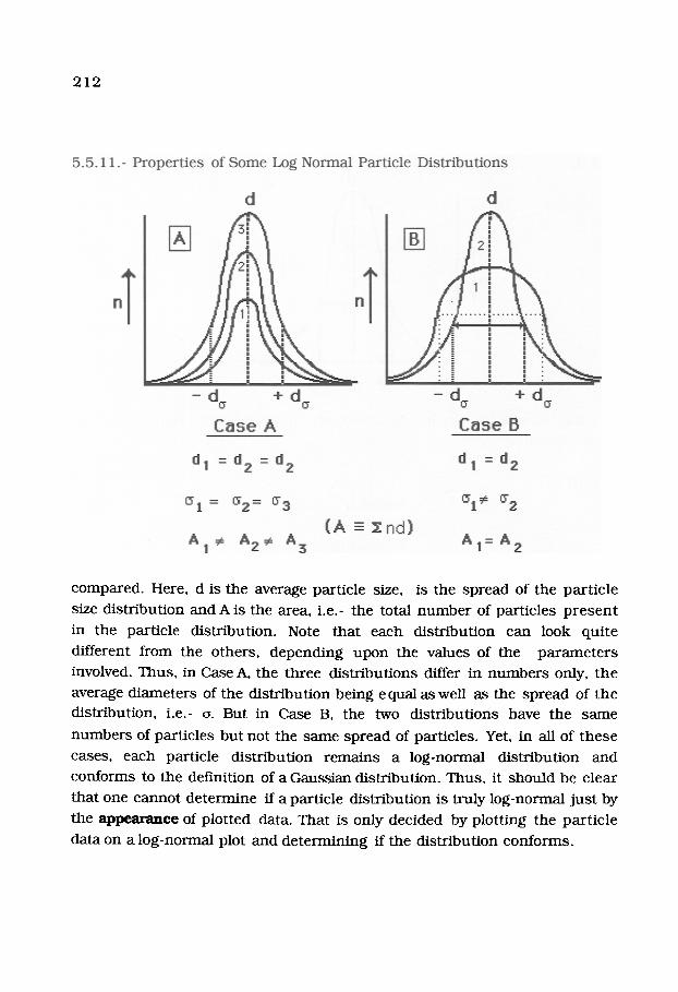
212

compared. Here, d is the average particle size, is the spread of the par t ic le

size distr ibution and A is the area, i.e.- the total number of particles p r e s e n t

in the particle distribution. Note that each distr ibution can look quite

different from the others, depending upon the values of the pa r ame te r s

involved. Thus, in Case A, the three distr ibut ions differ in numbers only, the

average diameters of the distr ibution being equal as well as the spread of the

distribution, i.e.- o. But in Case B, the two distr ibut ions have the same

numbers of particles but not the same spread of particles. Yet, in all of these

cases, each particle dis tr ibut ion remains a log-normal distr ibution and

conforms to the definition of a Gaussian distribution. Thus, it should be clear

that one cannot de termine if a particle distr ibution is truly log-normal jus t by

the appearance of plotted data. That is only decided by plott ing the par t ic le

data on a log-normal plot and de termining if the distr ibution conforms.

2 1 3

5 . 6 , - MEASURING PARTICLE DISTRIBUTIONS

Our nex t t a s k is to d e t e r m i n e how to m e a s u r e a PSD. We k n o w tha t we can

specify a m e a n d iame te r , bu t how do we ob ta in it? The following is a s i m p l e

example i l lus t ra t ing one m e t h o d of doing so.

S u p p o s e we ob ta in a s ample of b e a c h sand . F r o m 5.3.3 . , we can see t ha t t h e

par t i c les are liable to range f rom about 8la to 2 4 0 0 ~. In o rde r to gene ra t e a

PSD, we m u s t s epa ra t e the par t ic les . One way we can s epa ra t e s u c h p a r t i c l e s

is by seiving them. But we find t ha t seives are only available in ce r ta in sizes,

as s h o w n in the following:

5 .6 .1 . - COMPLETE LISTING OF ALL SEIVE SIZES AVAILABLE- (U.S. STD.)

Seive No. Microns P e r m i s s i b l e Seive N0. M i c r o n s P e r m i s s i b l e

Variat i0n{%} . . . . . . . . . . . . . . . . . . . . . . . . . Var ia t ionf%)

3 .5 5 6 6 0 • 3 40 4 2 0 • 5

4 4 7 6 0 • 3 4 5 3 5 0 • 5

5 4 0 0 0 + 3 5 0 2 9 7 • 5

6 3 3 6 0 • 3 6 0 2 5 0 • 5

7 2 8 3 0 • 3 70 2 1 0 • 5

8 2 3 8 0 +_ 3 8 0 177 • 6

10 2 0 0 0 + 3 100 149 • , , , , , , . . . .

12 1 6 8 0 • 3 170 88 +

14 1 4 1 0 • 3 2 0 0 7 4 •

16 1 1 9 0 • 3 2 3 0 62 •

18 I 0 0 0 • 5 2 7 0 53 •

20 8 4 0 • 5 3 2 5 4 4 + 7

25 7 1 0 • 5 4 0 0 37 • 7

3 0 5 9 0 +_ 5

35 6 0 0 + 5

2 1 4

T h e r e are two types of s t a n d a r d s c r e e n s , the U.S. a n d the Tyler s t a n d a r d

s c r eens . We have given the U.S. s c r e e n values. Those of the Tyler are ve ry

s imilar , e.g. - #5 Tyler = 3 9 6 2 ~ , # 20 = 833 ~, a n d # 4 0 0 = 38 p.

To s c r e e n ou r s a n d sample , we choose to employ the following seives:

#10, # 18, #20 , #30, #40, #50, #80, # 1 0 0 ,

#170 , #200 , #270 , # 3 2 5 & # 4 0 0 .

Now ff we s c r e e n the s a n d wi th the # I0 sc reen , all pa r t i c l e s l a rger t h a n

2 0 0 0 + 60 p will be r e t a i a e d u p o n the sc reen . The nex t s tep is to r e s c r e e n

the p a r t t h a t I m a ~ d t h r o u g h the # 10 sc reen , u s ing the # 18 sc reen , to obta in

a f r ac t i on w h i c h is > 1000 ~ + 50p. We t h e n r e p e a t th i s p r o c e d u r e to ob ta in

a se r ies of f rac t ions . The r e s u l t s are given in the following:

5 .6 .2 . - F rac t ions Ob ta ined

fo > 2 0 0 0 p

l O001a < fl < 2 0 0 0 la

8401a < f2 < 1000

590ja < f3 < 840

m

Mean d i a m e t e r d

1500

9 2 0

7 1 5

420p < f4 < 590 p 5 0 5

297p < f5 < 4 2 0 p 3 5 8

177ja < f6 < 297 la

1491a < f7 < 177

88 Ja<f8 < 1491a

77 la < f9 < 88

53 ~ < flO < 77

4 4 j a < f l l < 53

37 p < f12 < 44

2 3 7

163

118

83

68

4 9

41

do

d l

d2

d3

d4

d5

d6

d7

d8

d9

dlO

d l l

d12

do f13 < 37 lu

2 1 5

We now have 12 f rac t ions t ha t we can use. The m e a n d i a me te r is a p p a r e n t

f rom the s c r e e n s u s e d to s epa ra t e the f ract ions. In the las t case tha t we can use, d'-12 = 4 1 + 2 . 8 ~ . We can now w e i g h each f ract ion a nd calcula te the %

weigh t in each fract ion, p rov id ing we use the total weigh t of all 14 f rac t ions .

Knowing the dens i ty of the sand , a n d a s s u m i n g the par t ic les to be s p h e r e s ,

we can t h e n obta in the n u m b e r of par t ic les in each fract ion. (Note tha t w e

have a s s u m e d tha t all par t ic les smal l enough to p a s s t h r o u g h a given s c r e e n

have done so. In m a n y cases , th is is not t rue , a nd we have to be cognizan t of

th i s e ~ o r , i.e.- t h i s factor is the m a i n source of e r ror in the SIEVE

METHOD of par t ic le size analysis). We now find t h a t t he re are two g e n e r a l

m e t h o d s for da t a - r epor t ing , namely :

5 .6 .3 . - METHOD I = % of total w e i g h t

METHOD II = Cumulat ive w e i g h t - %

Each has i ts advantages . In the first m e t h o d , we calcula te the total w e i g h t

a n d ass ign each f ract ion a %-value. Mean d i a m e t e r s , d', a re easy to obta in in

the first m e t h o d b e c a u s e we k n o w the sc reen d i a m e t e r s u s e d to s epa ra t e t h e f ract ions. In the second, we add f2 to f l , t h e n f3 to f2 + f l , t h e n f4 to f3 +

f2 + fl, etc. To ob ta in d' , we t ake t he average of the added fract ions, s h o w n

as follows:

m

5 .6 .4 . - d

fl 1500 ~I

f2 + fl 1 2 1 0

f 3 + f 2 + fl 9 6 3

f4 + f 3 + f 2 + f l 7 3 4

We con t i nue wi th all the f rac t ions we have. If we now plot the data, we ge t

the d iagram, given as 5.6.5. on the next page.

2 1 6

We can see the sp read of par t ic les in Method I, bu t canno t d e t e r m i n e t he

m e a n accurately, s ince d" is a guess . Method II allows us to obta in the m e a n

from the 50% point , t ha t is, the point where 50% of the par t ic les are

smal ler than , and 50% are larger than.

Actually, the da ta of Method I are be t t e r p lo t ted as shown in the following

diagram:

217

Method III is called a "Histogram Plot" while Methods I & II are cal led

"Frequency Plot" and "Cumulative Frequency Plot", respectively. There is one

impor t an t po in t which needs to be emphas ized . Tha t is:

"ALL METHODS FOR PRESENTING DATA FROM THE MEASUREMENT OF

PARTICLE SIZE DISTRIBUTIONS, WHETHER INSTRUMENTAL, SEIVING,

SEDIMENTATION, OR PHOTOMETRIC METHODS, MEASURE FRACTIONS

OF THE TOTAL PARTICLE DISTRIBUTION. IF THE METHOD IS

SENSITIVE, THE F R A C T I O N - S E G M E N ~ CAN BE SMALL, AND T H E

MEASURED PARTICLE DISTRIBUTION WILL BE CLOSE TO THE ACTUAL

ONE. IF THE MEASUREMENT IS LESS SENSITIVE, THERE MAY BE

SIGNIFICANT DEVIATIONS FROM THE CORRECT PSD.

The data for the f rac t ion-s teps can be in t e rms of n u m b e r s of par t ic les ,

weight, %-weight or even a packed volume. We shall next invest igate

p a r a m e t e r s of d is t r ibut ions as a funct ion of m e t h o d of repor t ing data.

5.7, - AN/~YSIS OF PARTICLE DISTRIBUTION PARAMETERS

Each of the m e t h o d s of data p re sen ta t i on has its own special p rob lems in

t e rms of the a m o u n t of extractable informat ion one can obtain. We will

address each of these in turn , s ta r t ing vcith the least compl ica ted one, w h i c h

is the "His tog ram" .

A. THE HISTOGRAM

A typical h i s tog ram is shown in the following diagram, given as 5.7.1. on the

nexty page, along with an analysis of the p a r a m e t e r s which can be calculated.

The first s tep is to calculate the individual areas of the steps, Ai. These are

s u m m e d and then divided by the n u m b e r of individual areas, and t h e n mul t ip l ied by the s u m of (d2 - d l ) ! ni to find the mean , d . Admittedly, t he

m e t h o d is cumber some , bu t some t imes this is all the data we have.

2 1 8

5 .7 .1 . -

! 0 0

% of

Total 5 0

Weight

Ai - ~ ; l :d2_ d I )

d = I A i l n . �9 I ( d 2 - d m

d

t ) /ni

B. FREQUENCY PLOTS

Many pa r t i c l e -measu r ing m e t h o d s use STOKE'S LAW to d e t e r m i n e pa r t i c l e

d is t r ibut ions . By sui table manipula t ion{see below), we obta in an equa t ion re la t ing the Stokes d iameter , M, wi th the par t ic le density, P I ' and the l iquid

densi ty, P2' namely:

5.7.2.- M = 18 vl h / c~ t (p~ - P2 )g

where ~ is the liquid viscosity, h the d i s tance sett les, a is a shape factor (a =

1 for a spher ica l particle), and g is the gravi tat ional cons tan t . T h e

pho tome t r i c m e t h o d (which we shall d i scuss in more detail below) gives %

at a specific par t ic le d i ame te r and hence can be direct ly p lo t ted as

f requency, as given in the following d i ag ram which is labelled 5 .7 .3 . on t h e

next page.

As shown in the d iagram, do can be ca lcula ted from the m e a n d i ame te r if

the d is t r ibut ion is symmetr ica l , bu t th~-~r r a re ly are. Note also tha t o, which is

defined as the d i ame te r l imits equal to 68% of the total par t ic le populat ion, canno t be obtained, only d o .

2 1 9

C. CUMULATIVE FREQUENCY

The m o s t p o p u l a r m e t h o d of da ta p r e s e n t a t i o n

f requency . An example of th is is s h o w n as follows:

is t ha t of cumula t ive

m

Note t ha t bo th d and o are easily ob ta ined . But no o the r in fo rma t ion can be

derived. Wha t we need is a m o r e versa t i le m e t h o d . This can be a c c o m p l i s h e d

2 2 0

by cons ide r ing a m e t h o d re la ted to the stat is t ical na tu r e of near ly all pa r t i c l e

d is t r ibut ions .

The mos t versat i le m e t h o d for displaying and analyzing par t ic le size

d is t r ibut ions is by plot t ing t h e m as a log n o r m a l d is t r ibut ion . What th is

m e a n s is tha t we use log norma l probabi l i ty pape r to plot the data. It is th is

m e t h o d tha t we shall invest igate in detail s ince it p roduces informat ion about

the d is t r ibut ion n o t obtainable by any o ther me thod . In fact, one can

d is t inguish be tween na tura l and artificial PSD's and m a k e i n f e r e n c e s

conce rn ing the origin of the PSD. Also, we can easily d is t inguish the b imoda l

case , i.e.- two PSD's p r e s e n t at the same time. Th i s is imposs ib le o t h e r

m e t h o d s of da ta p r e s e n t a t i o n .

D. I.J3G NORMAL PROBABILITY METHOD

Consider the log no rma l (Gaussian) dis t r ibut ion, of which an example is given

as follows:

Our app roach is to a s sume tha t all PSD's have an origin in growth tha t t e n d s

to p r o d u c e a log norma l populat ion. This is reasonable s ince near ly all, if no t

all, par t ic le growth m e c h a n i s m s are r a n d o m in na ture . Hence, we expect to

221

see a log normal PSD as the usual case. What we then do is to look for

devia t ions f rom log normal i ty . It is these aber ra t ions which supply addi t ional

informat ion about the PSD.

To plot a dis t r ibut ion, we use log probabil i ty paper . ,an sample is given in t he

following diagram:

A log normal d is t r ibut ion will give a s t r a igh t l ine when plot ted on this type of

paper . This m e a n s tha t the PSD is not l imi ted, i.e.- all sizes of part ic les are

p r e sen t from - ~o to +~o. However, ff the PSD is g rowth - l imi t ed , it will readi ly

appa ren t from the graph. Ostwald r ipening, a m e c h a n i s m where large

2 2 2

par t ic les grow at the expense of small ones, is one m e c h a n i s m tha t can give

rise to growth limits. Growth limits are denoted by:

5 . 7 . 7 . - ._..~

L- L I """T

Xo

Upper Growth Limit

Lower Growth Limit

- Upper Discontinuous Limit

- Lower Discontinuous Limit

The d i scon t inuous limit is tha t in which all par t ic les beyond a specific size

have been removed, or do not exist. The d iamete r of the par t ic les is found

on the y-axis and plot ted at the p roper point on the x- axis as "% less than"

(see Method II of 5.6.3. and 5.7.4., given above).

5 .8 - TYPES OF LOG NORMAL PARTICLE DISTRIBUTIONS

We shall p r e sen t some examples of part icle d is t r ibut ions and how to

in te rp re t t h e m in order to show the versati l i ty of the method . As you will

see, the m e t h o d of plot t ing part icle d is t r ibut ions via a log-normal m e t h o d

allows one to in te rp re t part icle size in a m a n n e r not feasible by o t h e r

me thods . Yet you will find tha t mos t part icle size special is ts do not take

advantage of the m e t h o d .

A. UNLIMITED PARTICLE DISTRIBUTIONS

The following diagram, given as 5.8. I. on the next page, shows a typical PSD

where the d is t r ibut ion does not have l imits.

2 2 3

Fol lowing th i s e x a m p l e are d i s t r i bu t i ons t h a t do have l imi t s to the "normal"

d i s t r ibu t ion . Wha t th i s m e a n s is t h a t the d i s t r i bu t i ons c o n f o r m to the l im i t s

def ined in 5 .7 .6 . Note t h a t in 5 .8 .1 . , a s t r a igh t l ine is evident . This is t h e

type of d i s t r i bu t ion usual ly found as a r e su l t of m o s t p r e c i p i t a t i o n p r o c e s s e s .

But as we shal l see, th i s is no t t rue for the o t h e r types of l o g - n o r m a l

d i s t r i bu t i ons .

B. LIMITED PARTICLE DISTRIBUTIONS

If a p r e c i p i t a t e is a l lowed to u n d e r g o Os twa ld r ipen ing , or is s in t e r ed , or is

c a u s e d to e n t e r in to a solid s t a t e r eac t ion of s o m e k ind , it will of ten deve lop

into a d i s t r i bu t ion w h i c h has a size l imit to i ts g rowth . T h a t is, t he r e is a

m a x i m u m , or m i n i m u m l imi t (and s o m e t i m e s b o t h ) w h i c h the p a r t i c l e

d i s t r i bu t i on a p p r o a c h e s . The d i s t r i bu t i on r e m a i n s c o n t i n u o u s as i t

a p p r o a c h e s t h a t l imit . The log-probab i l i ty plot t h e n has the form s h o w n in

5 .8 .2 . on the nex t page .

In th is case , b o t h u p p e r a n d lower l imi ts are shown. However , one m a y have

one or the o ther , or bo th , in the general case . Os twald r i p e n i n g t e n d s to use

2 2 4

up all of the smal l par t i c les , w i t h o u t l imi t ing the u p p e r size. T h e n we w o u l d

have the lower l imit b u t no t the u p p e r .

C. PARTICLE DISTRIBUTIONS WITH DISCONTINUOUS LIMITS

S u p p o s e we use a 2 0 0 - m e s h s c r e e n to r emove pa r t i c l e s la rger t h a n 74~ and

a 4 0 0 - m e s h s c r e e n to r emove t hose sma l l e r t h a n 37V. The PSD is t h e n :

225

Note tha t the d is t r ibut ion is l inear be tween 37 and 74 ~ but tha t it abrupt ly

shifts to + oo at these points . This is a part icle d is t r ibut ion for which it is

impossible to obtain an accura te p ic ture by any o ther means .

A frequency plot of the s a n e data would look like t h e n look like this:

If we w e r e us ing the f requency plot m e t h o d to p r e sen t this data, we would

th ink tha t the curve was jus t a s symmet r ica l and tha t the d is t r ibut ion was no t

log-normal. Yet, it is obvious from 5.8.3. tha t it is log-normal .

D. MULTIPLE PARTICLE DISTRIBUTIONS

Log probabil i ty plots are par t icular ly useful when the d is t r ibut ion is bimodal ,

tha t is, w h e n two separa te d is t r ibut ions are presen t . Suppose we have a

d is t r ibut ion of very small part icles, say in su spens ion in its m o t h e r liquor. By

an Ostwald r ipen ing mechan i sm , t he small par t ic les redissolve and

reprec ip i ta te to form a d is t r ibut ion of larger part icles. This would give us t he

d is t r ibut ion shown in 5.8.5. on the next page.

226

In this illustration, the size distr ibution parameters of both distr ibut ions are

readily apparent . A similar de terminat ion is almost impossible with o the r

types of data presenta t ion methods . Although a large d i ~ o a t i a u o u s gap

between the two distr ibut ions is shown in 5.8.5., it is rarely the case.

As examples of the usefulness of particle distr ibutions, consider the

following. Two actual cases encounte red in Indust ry are described in the

following examples:

CASE I - FLUORESCENT LAMP PHOSPHOR PARTICLES

Fluorescent lamps are manufac tured by squir t ing a suspens ion of p h o s p h o r

particles in an ethyl cellulose lacquer upon the inner surface of a vertical

glass tube. Once the lacquer drains off, a film of particles is formed. The

lacquer is then burned off, leaving a layer of phosphor particles. E lec t rodes

are sealed on; the tube is evacuated; Hg and inert gas is added; and the lamp

ends are added to finish the lamp. Lamp br ightness and lifetime are

dependen t upon the particle size distr ibut ion of the phosphor particles. The

number of small particles is critical since they are low in br ightness output

227

bu t high in light sca t t e r ing and absorpt ion. A lamp b r igh tne s s i m p r o v e m e n t

of 10% is easily achieved by removal of these par t ic les . In 5.8.6. is shown t h e

PSD tha t r e su l t ed w h e n a cer ta in mechan i ca l m e t h o d was used to r e m o v e

the "fines", viz-

In this appl icat ion of the log-normal plot, note tha t the "mechanica l" separa t ion of "fines" has c rea t ed a new par t ic le d is t r ibut ion wi th d2 = 2 p.

Even the value of 02 differs f rom tha t of the major par t ic le dis t r ibut ion. In

the "fines" fraction, it appea r s tha t the larges t par t ic le does not exceed about

5 p. Needless to say, l amps p r e p a r e d from this p h o s p h o r were inferior in

b r igh tness . Armed with this informat ion, one could then r e c o m m e n d tha t

the m e t h o d of "fines" removal be changed .

Another case is p r e s e n t e d on the next page.

CASE II. - TUNGSTEN METAL POWDER

The l ifet ime of a t u n g s t e n f i lament in an i n c a n d e s c e n t l ight bulb d e p e n d s a

grea t deal on the gra in size of the wire u sed to m a k e the f i lament. W-meta l

powder is p r e s s e d into a bar at p r e s s u r e s which ensu re tha t the dens i ty is as

228

close as possible to the theoretical density. The bar is s intered in an iner t

a tmosphere and then "swaged" , i.e.- "hammered" into a long rod. This rod is

then drawn into a fine wire (~ 2-5 mil) which is wound into the f i lament

form. Metal powder particle size has a major effect upon wire quality s ince

fine particles form small grs.hm in the wire while large part icles will form

ulrge grains.

When the filament is operated at 3250 ~ to produce light, the wire is hot

enough that vacancy migrat ion will occur in the wire. Simultaneously, grain

growth plus an increase in grain size also occurs. The grain boundar ies

between large grains will "pin" vacancies, but grain boundar ies between small

grains do not appear to do so. If they do, the effect is at least an order of

magni tude smaller. As the vacancy concent ra t ion builds up at the large grain

boundar ies (see the Kirchendall effect given in Chapter 4), local res is tance to

electron flow increases. Eventually, a "hot spot" develops and the tungs ten

wire melts at that point, with consequent failure of the filament and the

lamp. If only small metal particles are used to make the wire, then the small

grains produced m u s t grow into large grains before "hot spots" cause its

eventual fa i lure . Therefore, incandescen t lamp manufac turers exercise very

close control of the tungs ten-meta l powder PSD and the s inter ing p rocesses

used to produce the wire to eliminate, as much as possible, pores and

control actual density. The diagram shown as 5.8.7. on the next page

i l lustrates a typical PSD for a tungs ten metal powder where the large

particles have been removed. In this case, the PSD is suitable and par t ic les

larger than about 5 ~ appear to have successfully removed.

This completes the types of particle dis tr ibut ions that we might encounter .

It is now time to show how particle size count ing-data are used. To do this,

we m u s t select an i n s t rumen t tha t produces counts of size of par t ic les

correlated with numbers of particles in each size range. There are several

types of such in s t rumen t s whose na ture will be delineated below. But, first,

we mus t show how this is done. Let us now examine a me thod of calculating

a particel size distr ibution.

2 2 9

5.9- : A TYPICAL PSD CALCULATION

Let us suppose tha t we have a part icle count ing i n s t r u m e n t which sor ts and

coun ts the n u m b e r of par t ic les at a given part icle size. The e x p e r i m e n t a l

data tha t we collect are:

Having obta ined the data as given in 5.9.1., our next s tep is to calculate t he

a ~ e size in each part icle intea-wal. For par t ic les less t han 2.2 ~, we have 2

2 3 0

pa r t i c l e s . At 3 .0 la, we have 4 pa r t i c l e s . T h e r e f o r e , in t h e r a n g e 2 .2 - 3 .0 ~,

we have t w o (2} p a r t i c l e s w h o s e ave rage size is 2 .6 p.

In the r a n g e 3 .0 - 5 .0 tJ, we have fou r (4} p a r t i c l e s w h o s e ave rage size is 4 . 0

~. We t h e r e f o r e c o n t i n u e to c a l c u l a t e An, as s h o w n in T a b l e 5 - I . for e a c h

size r a n g e t h a t we have m e a s u r e d :

TABLE 5 - 1

A TYPICAL PARTICLE SIZE DISTRIBUTION C A I ~ U I A T I O N

D i a m e t e r n - C o u n t s An d o % z%

2.2 ~1 0

2 2 .6 tl 0. I 0. I

4 2

2 4 4 . 0 1.2 1.3

5 . 0 2 8

2 0 4 6 . 0 10 .2 11 .5

7 . 0 2 3 2

3 7 0 8 . 0 18 .5 3 0 . 0

9 . 0 6 0 2

3 0 0 9 . 5 1 5 . 0 4 5 . 0

10 9 0 2

5 0 0 12 .5 2 5 . 0 7 0 . 0

15 1 4 0 2 , ,

5 0 0 2 0 . 0 2 5 . 0 9 5 . 0

2 5 1 9 0 2

8 0 2 7 . 5 4 . 0 9 9 . 0

3 0 1 9 8 2

18 3 5 . 0 0 . 9 9 9 . 9

4O 20OO

231

We have a total of 2000 par t ic les tha t we have m e a s u r e d and we can calcula te

the p e r c e n t (%) of total coun t s for each size range. This gives the following

log-normal PSD plot, viz-

Here, the p a r a m e t e r s of the d is t r ibut ion are given. This mate r ia l appea r s to

have been prec ip i ta ted , or it m a y have been ob ta ined by a g r ind ing p rocess ,

s ince the p a r a m e t e r s indica te a Gaussian un l imi t ed dis t r ibut ion. Par t i c les

grown by solid s ta te react ion, inc luding Ostwald r ipening, general ly have PSD

cha rac te r i s t i c s of the original PSD from which they were formed. Tha t is,

there will be Emits accord ing to the original d is t r ibut ion from which it has

ar isen.

If the original PSD had limits, t hen the p rogeny PSD ,;viii also have such

limits. The basis for this behavior lies in the fact tha t ff one s t a r t s wi th a

cer ta in size range of par t ic les as the basis of par t ic le reac t ion and g rowth ,

one will end with the same size range of par t ic les in the PSD of the pa r t i c l e s

p r o d u c e d by the solid s ta te react ion. Such a case is shown in the following

diagram, given as 5.9.3. on the next page. Here, the oxalate was p r e p a r e d by addi t ion of oxalic acid to Gd(NO3)3 solut ion to form a p rec ip i t a t e .

2 3 2

There is an uppe r limit of about 23 mic rons in size. This m a y be due to t he

fact tha t the p rec ip i ta t ion was accompl i shed at 90 ~ or from the fact tha t

ra re ea r th oxalates t end to form very smal l par t ic les dur ing p r e c i p i t a t i o n

which then grow via Ostwald r ipen ing and agglomera t ion to form la rge r

ones. Never theless , it is clearly evident tha t w h e n the oxalate is hea t ed at

e levated t e m p e r a t u r e (~ 900 ~ the oxide p r o d u c e d rctaln-q the same PSD

character is t ics of the original p r ec ip i t a t e .

5 .10. - METHODS OF MEASURING PARTICLE DISTRIBUTIONS

Having defined par t ic les and par t ica l d is t r ibut ions , we now examine m e t h o d s

by which we can m e a s u r e par t ic les and p roper t i e s of powders . There are

four (4) p r imary m e t h o d s used to obtain da ta conce rn ing par t ic le size

d is t r ibut ions . These include:

OPTICAL

SEDIMENTATION

PERMEATION

ELECTRICAL

ABSORPTION

233

A..The Microscope - Visual Count ing of Partic,!es

At the p roper magnif icat ion and with a special eye piece, one can d i rec t ly

m e a s u r e part icle d iameters . The eye-piece m u s t have i n t e r n a l l y - m a r k e d

concent r ic circles so tha t a given part icle will fall wi th in one or more of the

circles. The d iamete r then can then be read a n d / o r es t imated directly as

shown in the following:

In this case, three par t ic les are shown, a 40 ~, 20 ~ and a 10 ~ particle. T h e

mos t impor t an t s tep is sample p repara t ion on the mic roscope slide, s ince

only a p inch of mater ia l is used, one m u s t be sure tha t the sample is un i fo rm

and representative of the material . Also, since m o s t mater ia l s tend to

agglomerate due to accumula ted surface charge in a dry state, one adds a few

drops of alcohol and works it with a spatula, sp read ing it out into a th in layer

which dries. Too m u c h work ing b reaks down the original par t ic les ,

2 3 4

par t icular ly the larger ones, and too little work ing leaves agglomerates . With

a little pract ice, the p repara t ion of a p roper slide of par t ic les becomes easy.

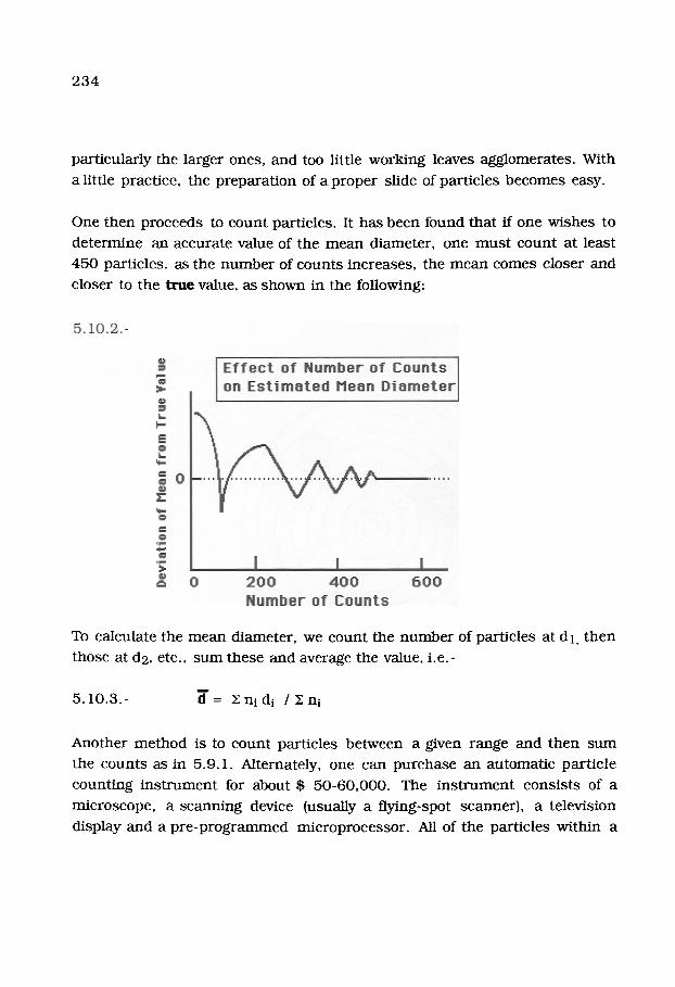
One then p roceeds to coun t part icles. It has been found tha t ff one wishes to

de te rmine an accura te value of the m e a n diameter , one m u s t coun t at least

450 part icles, as the n u m b e r of coun t s increases , the m e a n comes closer and

closer to the t rue value, as shown in the following:

To calculate the m e a n diameter , we count the n u m b e r of par t ic les at d I, t h e n

those at d2, etc., s u m these and average the value, i.e.-

5 .10 .3 . - m

I! = X n i d i / X n i

Another m e t h o d is to coun t par t ic les be tween a given range and then sum

the coun ts as in 5.9.1. Alternately, one can pu rchase an au tomat ic par t ic le

count ing i n s t r u m e n t for about $ 50-60 ,000 . The i n s t r u m e n t cons i s t s of a

microscope , a scann ing device (usually a flying-spot scanner) , a te levision

display and a p r e - p r o g r a m m e d mic roprocesso r . All of the par t ic les within a

235

given frame can be counted and grouped automatically. Thus, several f rames

per minute can be counted by an operator, or the in s t rumen t can be set to

operate automatically according to a prese t program. Since the i n s t r u m e n t

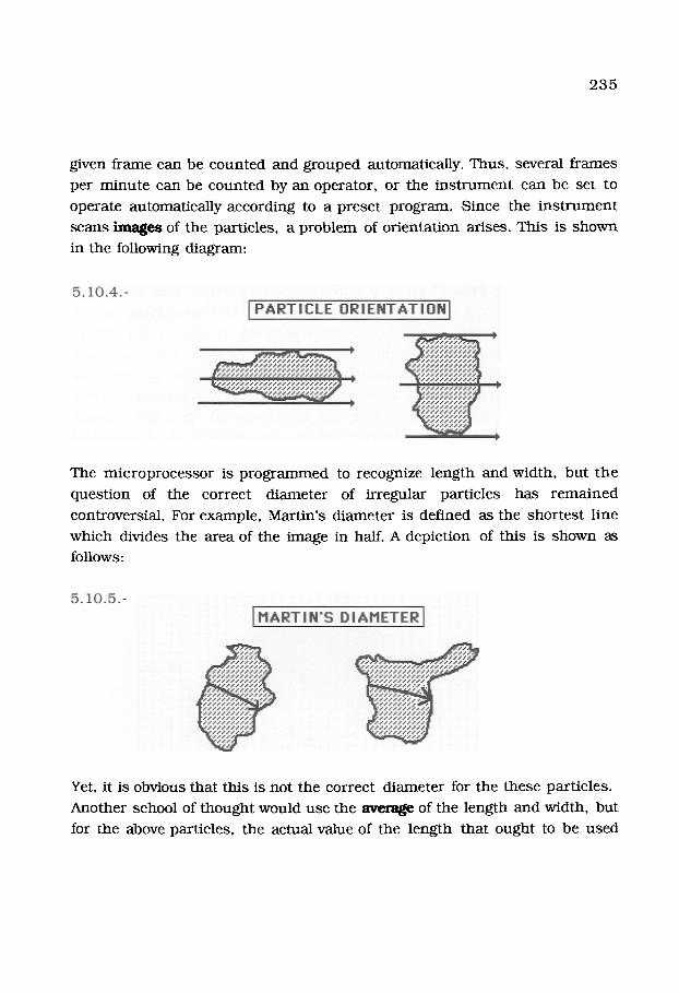
scans imagca of the particles, a problem of or ientat ion arises. This is shown

in the following diagram:

The mic roprocesso r is p rog rammed to recognize length and width, but the

quest ion of the correct d iameter of irregular particles has r ema ined

controversial. For example, Martin's diameter is defined as the shor tes t line

which divides the area of the image in half. A depiction of ~.is is shown as

follows:

Yet, it is obvious that this is not the correct diameter for the these part icles .

Another school of thought would use the a ~ e of the length and width, but

for the above particles, the actual value of the length tha t ought to be used

236

remains questionable. This problem has remained the most serious bar r ie r

to obtaining PSD by optical microscopy until recent ly.

With the advent of compute rs which can process data at the rate of 700

billion bits per second, this problem has been solved satisfactorily. This PSD

ins t rumen t {Malvern Ins t ruments , 10 Southville Road, Southborough, Ma.

01772 - Sysmex FPIA-2100) is a fully au tomated particle size mad ~hape

analyzer. It uses CCD, i.e.- "charge-coupled device", technology (the optical

basis of a digital video camera) to capture a series of images of par t ic les

suspended in a liquid medium. Particles are sampled from a dilute

suspension which is forced through a "sheath-flow" cell. This insures that

the largest area of the particle is or iented toward the video camera and that

all of the particles are in focus. The cell is i l luminated via a s t roboscopic

light source and images are cap tured at 30 Hz. per second. A c o m p u t e r

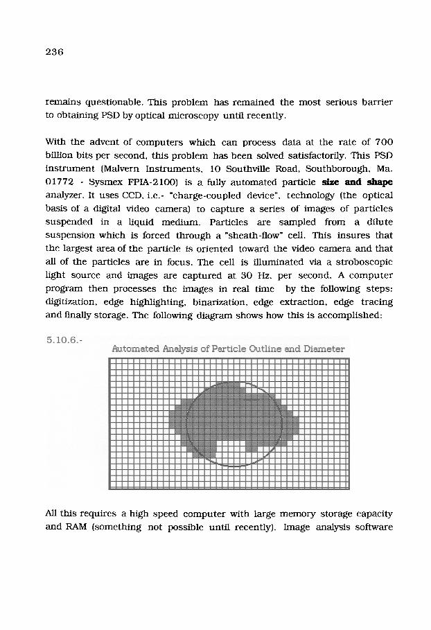
p rogram then processes the images in real time by the following steps:

digitization, edge highlighting, binarization, edge extraction, edge t rac ing

and finally storage. The following diagram shows how this is accompl ished:

All this requires a high speed compute r with large memory storage capacity

and RAM (something not possible until recently). Image analysis software

237

then calculates the area and per imeter of each of the captured Lnaages and

then calculates the particle diameter and circularity. The particle shape is

easily recognized in this diagram. The area of the circle is equal to that of

the digitized particle so that the particle circularity (shape) can be classified.

Circularity, C, is de te rmined by:

5 .10.7 . - C = per imeter of circle / per imeter of par t ic le

Once the m e a s u r e m e n t is complete, the particle size and circularity can be

displayed in both graphical and table form. A typical repor t includes: par t ic le

size distribution, circularity distr ibution and a sca t te rgram of particle size vs:

circularity. All these can be displayed and pr in ted in hard copy. Individual

particle images can be displayed and then classified into categories

including uni-particle, hi-particle, and agglomerate, This ra ther new

ins t rumen t has solved the problem of particle shape and cor responding size

through optical digitization me thods .

B. SEDIMENTATION METHODS

There are several particle sizing methods , all based upon sedimenta t ion and

Stokes Law. If a particle is suspended in a fluid (which may be gas, or any

liquid), the force of res is tance to movement by the particle will be

proport ional to the particle 's velocity, v, and its radius, r, vis-

5.10.8- f = 6n r ~ v

where ~ is the viscosity of the fluid, providing the particle is spherical. If

the particle settles under the influence of gravity, then we can write:

5 .10.9 . - f = 4 / 3 / n r 3 (Ps - P l ) g = 6 n r ~ i v

where ps and pl are the densit ies of the solid particle and the liquid,

respectively. Since the distance sett led is: h = v t, then:

238

5 .10 .10 - d = { 18~l h / a t ( p s - P l ) g } l / 2

This is S tokes Law for s ed imen ta t ion where we have added a , a shape factor,

jus t in case we do not have spher ica l part icles. For spheres , r = 1. It is

fractional o the rwise .

One way to m e a s u r e par t ic les is to weigh t h e m as they settle out f rom

suspens ion , such an appara tus is called a "sed imenta t ion balance" and is

des igned as shown in the following diagram:

The weight of the par t ic les bui lds up with t ime and is p ropor t iona l to I / d . If

we as sume spher ical par t ic les , then we can convert the above curve to

part icle d iameter from Stokes Law. Although we have added the par t ic le

suspens ion to a "water cushion" as shown above, it migh t not seem tha t the

set t l ing of the part ic les would str ict ly adhere to Stokes Law, which as sumes

the te rminal velocity to be cons tan t .

But, as shown in the following Table, the approx imate d is tance a par t ic le

needs to travel to reach te rminal velocity in a given l iquid is very shor t .

2 3 9

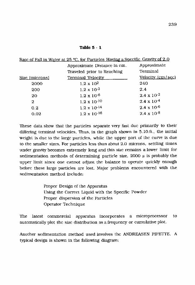
Table 5 - 1

Rate of Fall in Water at 25 ~ for Par t ic les Having a Specific Gra,~ity of 2 .0

Approximate Dis tance in cm. A p p r o x i m a t e

Traveled pr ior to Reach ing T e r m i n a l

Size ( m i c r o n s l Te rmina l Veloci ty Velocity_ ( c m / s e c l

2 0 0 0 1.2 x 102 2 4 0

2 0 0 1.2 x 10 -2 2 .4

2 0 1.2 x 10 -6 2.4 x 10 -2

2 1.2 x 10 -I0 2.4 x 10 -4

0 .2 1.2 x 10 -14 2.4 x 10 .6

0 . 0 2 1.2 x 10 -16 2.4 x 10 -8

These da ta show tha t the par t ic les sepa ra t e very fast due pri_mm-ily to t h e i r

differing t e rmina l velocities. Thus , in the g r aph shown in 5.10.9. , the init ial

weight is due to the large par t ic les , while the u p p e r pa r t of the curve is due

to the smal ler sizes. For par t ic les less t h a n about 2.0 microns , se t t l ing t i m e s

u n d e r gravity becomes ex t remely long and this size r e m a i n s a lower l imit for

s ed imen ta t i on m e t h o d s of d e t e r m i n i n g par t ic le size. 2000 ~ is probably t h e

u p p e r limit s ince one canno t adjus t the ba lance to opera te quickly enough

before these large par t ic les are lost. Major p rob lems e n c o u n t e r e d with t he

s ed imen ta t i on m e t h o d include:

Proper Design of the Appara tus

Using the Correct Liquid with the Specific P o w d e r

Proper d i spers ion of the Par t i c l es

Opera to r T e c h n i q u e

The la tes t commerc i a l appa ra tus inco rpora te s a m i c r o p r o c e s s o r

automat ica l ly plot the size d is t r ibu t ion as a f requency or cumula t ive plot .

to

Another s ed imen ta t i on m e t h o d used involves the ANDREASEN PIPETTE.

typical design is shown in the following d iagram:

A

2 4 0

This glass appara tus is inexpens ive and cons is t s of a bot t le having an i n t e rna l

sampl ing tube and ca l ibra ted sampl ing volume (5 ml). One draws a sample

and then expels it into an ex te rna l 5 ml beake r .

Using the t imes ca lcu la ted for success ive d i ame te r s to set t le pas t the orifice,

one wi thd raws samples c o r r e s p o n d i n g to tha t d iameter . A ser ies of s amp le s are ob ta ined at t 1 , t 2 , etc., which are dried and weighed. The actual s amp le

ob ta ined is a na r row par t ic le d is t r ibut ion r a the r t han one Sl~cUlc size. Thus ,

the d i ame te r m e a s u r e d (by calculat ion) does not exactly c o r r e s p o n d to the

t rue Stoke 's d iameter , bu t to the peak of a na r row distr ibution.Yet , t he

Andreasen Pipet te m e t h o d con t inues to be the mos t widely used

s ed imen ta t i on m e t h o d since it involves inexpens ive equ ipmen t , and is

reasonably accura te if one will take the t ime to develop a c o r r e c t

expe r imen ta l t echnique . The reproducib i l i ty can be excellent , the accuracy

less so.

241

Another s ed imen ta t i on m e t h o d used is the so-cal led MSA-analyzer. If t he

value of "g" in 5.10.8. is i nc reased (such as the use of a centr i fuge) one can

analyze the very small par t ic les in tony given d is t r ibu t ion in a shor t t ime. T h e

p rob lem of course lies in accura te d e t e r m i n a t i o n of the weight a ccumula t ed

at a given t ime u n d e r a specific cen t r ipe ta l force. This p rob lem has b e e n

neat ly solved by careful design of the s ed imen ta t i on tube, as shown in t he

following diagram:

5 .10 .13 . -

Calibraled Stem

A SED I MENTAT I ON

TUBE

The par t ic les bui ld up by l a y e ~ because it has been found tha t all m o n o s i z e d

par t ic les can be removed from suspens ion by ro ta t ing at a specific speed .

Thus , one r u n s the i n s t r u m e n t at a ser ies of ro ta t ional speeds , m e a s u r i n g t he

weight of the bui ld-up layers in be tween each run. The overall analysis is r un

at specif ied rpm ' s which c o r r e s p o n d to se lec ted par t ic le d i a m e t e r s ,

r esu l t ing in da ta sufficient to cha rac te r i ze the par t ic le d is t r ibut ion .

C. ELECTRICAL RESISTIVITY - THE COULTER COUNTER

P e r h a p s the mos t useful m e t h o d for d e t e r m i n i n g par t ic le d is t r ibu t ions is

tha t of electr ical conductivi ty, the mos t widely used i n s t r u m e n t is t he

Coulter Counte r (named after the Inventors) , a l though there are now o t h e r

s imilar i n s t r u m e n t s on the marke t . Originally, this i n s t r u m e n t was d e s i g n e d

to m e a s u r e blood corpusc les which are 2-8 p in size. It has proven to be very

242

suited to measure micron and submicron particles easily, accurately, and

reproducibly.

Consider a conductive solution consis t ing of water with a soluble salt, i.e.-

1% NaCI, and a dispersing agent used to prevent agglomeration of par t ic les

in suspension. Two electrodes are placed in solution with a non-conduc t ing

orifice between them, as shown in 5 .10 .14 , given on the next page:

A ceramic block such as alumina is generally used because of its chemica l

iner tness and the orifice is bored or drilled to precise dimensions. The

block is placed so that two (2) chambers result. Then ff a DC voltage is

applied across the electrodes, a cur ren t will flow r th rough the orifice,

and an effective resis tance arises which depends upon the voltage applied

and the size (volume of the conduct ing solution) of the orifice. Particles are

added to one side of the two chambers created by the ceramic block, and

the suspens ion is pumped through to the other side. There will be an

electrical pulse as each particle passes through the orifice.

A depiction of the pulses obtained is shown in the following diagram, given

as 5.10.15. on the next page. Each pulse will be proport ional to the size of

the particle because the particle volume displaces par t of the conduc t ing

solution during its passage through the orifice. If we have proper ly

established steady state condi t ions ,

2 4 3

5 .10 .15 . -

TMO v ab i e hreshold

Counting

l

Non-counting

IDisplayed Pulses - COulter CounterJ

we will obtain a drop in c u r r e n t as each par t ic le passes th rough .

Electronical ly, this can be conver ted to a positive pulse whose in tens i ty is

p ropor t iona l to each par t ic le volume. We asmime s p h e r i c i t y of t h e par t ic les ,

If V is cons tan t , then :

5 .10 .16 . - I = V /AR a n d : A R = r o V p / A 2 - 1/ {1/1- (ro/re)} - a / A

where ro is the actual par t ic le radius , re is the effective rad ius ( incase the

par t ic le is not spheroid}, Vp is the volume of the part icle, A is the c ross -

sect ional a rea of the orifice, and a is a cons t an t which d e p e n d s upon the

solvent and solute u sed to m a k e the conduc t ing solution.

The size of the orifice m u s t be fi t ted to the r ange of par t ic les p resen t . If t he

par t ic les are too large, they will no t pass t h rough the orifice. Too small and

the pulse is not easily de tec ted , Since large n u m b e r s of par t ic les can be

p resen t , the powder con ten t m u s t be control led. Too high a pa r t i c l e

c o n c e n t r a t i o n - d e n s i t y will r esu l t in "coincidence counting". Tha t is, two

small par t ic les can be coun ted as one larger one. This p h e n o m e n a has b e e n

2 4 4

a d d r e s s e d and tables are provided to cor rec t for inc idence count ing. T h e

e lect ronic pa r t of the Coulter Counte r has several h u n d r e d "channels" to

accept pulses . The " threshold" is electrical , and mowable, so tha t one coun t s

the large par t ic les ffrrst (large pulses) and then moves the t h re sho ld lower to

coun t the smal ler par t ic les . The th re sho ld is actually a pulse he ight analyzer

which conver t s he ights to n u m b e r s . The da ta ob ta ined are easily c o n v e r t e d

to a f requency plot or a cumula t ive plot. Since fur r e sponse is l inear, one can

readi ly cal ibrate the i n s t r u m e n t at one point, us ing monos ized par t ic les such

as pollen or specially p r e p a r e d plast ic par t ic les . The only r e q u i r e m e n t is

tha t the cal ibrat ing par t ic les ought to be in the range of the par t ic les to be

m e a s u r e d .

The Coulter Counter is par t icu lar ly useful and un ique in tha t s teps as small as

1.0 mic ron may be used if so desired. Resul ts by this au tho r have

d e m o n s t r a t e d tha t some d i s t r ibu t ions which appea r to Gaussian m a y actually

consis t of more t han one subdivis ion where the peaks are s epa ra t ed by only a

few microns , an example is given as follows:

5. I0 .17 . - A PARTICLE DISTRIBUTION WITH SUB-DISTRIBUTIONS

This resu l t was achieved with a se lec ted par t ic le d is t r ibut ion w h i c h

originally appea red to be a single Gaussian dis t r ibut ion. When the pa r t i c l e

245

measur ing steps were changed so that a range of about 1-2 microns was

covered, the above resul t was obtained. Even so, the m e a s u r e m e n t mus t be

done carefully to reveal the subs t ructure . To the author 's knowledge, no

other me thod has the capability of such precision in particle d i ame te r

measuremen t . The latest Coulter Counter instanm~ents incorporate a

microprocessor and the operator can specify the form of the output data to

be obtained. The i n s t rumen t converts count -da ta to practically any format

desired, with the exception of log-probability plots.

D. OTHER METHODS OF MEASURING PARTICLE SIZE

Permeabi l i ty is another me thod for obtaining information about par t ic le

diameters. If one packs a tube with a weight of powder exactly equal to its

density, and applies a calibrated gas pressure th rough the tube, the p re s su re

drop can be equated to an average particle size. The in s t rumen t based on

this principle is called the "Fisher Sub-Sieve Sizer TM'. Only one value can be

obtained but the me thod is fast and reproducible. The in s t rumen t itself is

not expensive and the me thod can be applied to quality control problems of

powders. Pe rmeamet ry is useful in the particle range of 0.5 to 50 p.

Gas adsorp t ion is one other me thod somet imes used for de termining average

particle size. In this case, one is usually in teres ted in the surface area of a

powder and calculates the average size of the particles secondarily. The

me thod is called the BET-method after its developers, Brunauer, E m m e t t

and Teller. The procedure is t ime-consuming and is accomplished as

follows. A gas analysis train is used in which gas volumes can be recycled and

measu red very accurately. A we ighed sample is placed in the sample tube

and allowed to come to equilibrium. Since all solid mater ials have a

monolayer of water on the surface of the particles (we live in a wet world) ,

the sample is heated to 300 ~ to expel the water, in a ni t rogen gas flow.

Next, it is cooled to liquid ni t rogen tempera ture . At this point, the sample will adsorb a monolayer of N2-gas molecules on the surface of each part icle.

By allowing the t empera tu re of the sample to re tu rn to room t empera tu re ,

2 4 6

whi le m e a s u r i n g the v o l u m e of n i t rogen gas re leased , one ob ta ins a value

w h i c h can be c o n v e r t e d to a sur face a rea of the pa r t i c l e s be ing m e a s u r e d . In

p rac t i ce , one recyc les the s y s t e m several t imes , m e a s u r i n g a d s o r p t i o n and

d e s o r p t i o n v o l u m e s success ive ly so as to ob ta in an average value. It is found

t h a t the unoccupied f rac t ion of the s u r f a c e ( l - y) a p p r o a c h e s a c o n s t a n t value

w h e r e it is a s s u m e d t h a t y = 0. Ni t rogen gas is e s sen t i a l s ince it is the only

gas w h i c h forms m o n o l a y e r s easi ly w i t h o u t the t e n d e n c y to form m o r e t h a n

one layer of gas m o l e c u l e s on the surface . If the gas p r e s s u r e is k e p t b e t w e e n

s t r i c t l imits , the BET equa t ion is:

5 . 1 0 . 1 8 . - pg / ( V g [ 1 - p g ] = 1/ {Vmono " C) + {C- 1) pg /{Vmono " C)

where : C = exp { (FAds. - FCond.) / RT} , a n d pg is the gas p r e s s u r e . Vg is

the gas vo lume m e a s u r e d ; Vmono is the gas vo lume of the m o n o l a y e r

ca l cu l a t ed f rom the k n o w n d i m e n s i o n s of the n i t r o g e n - g a s molecu le s ; FAds.

is the Gibbs free ene rgy of adso rp t ion , a n d FCond. is the free ene rgy of

c o n d e n s a t i o n , pg is m e a s u r e d as the ra t io of the equ i l i b r ium p r e s s u r e at

specif ic t e m p e r a t u r e s , i.e.- r o o m a n d l iquid n i t rogen t e m p e r a t u r e s .

It has b e e n found t h a t a plot of pg / {Vg [1-pg] vs: pg is l inear for the p r e s s u r e

r ange of 0 .05 to 0.4, wi th a s lope of (C - 1) / (Vmono �9 C ) a n d i n t e r c e p t of

1/ (Vmono " C ). Let us now do a s imple ca lcu la t ion u s ing BET da t a ob ta ined .

S u p p o s e we have a 20 gm. s a m p l e hav ing a dens i t y of 2.0. We m e a s u r e t h e

sur face a rea as 6 m 2 . F r o m the a rea of a sphe re , A = n D 2 , a n d the vo lume of

a sphe re , V = 4 / 3 n D 3 ,, we find the total vo lume of n s p h e r e s to be 10 cc,

i.e.- n{4 /3 n D3} = 10. The sur face a rea of n{nD 2} s p h e r e s is 6 m 3. The to ta l

n u m b e r of s p h e r e s p r e s e n t , n, is the s a m e in bo th formulas . There fore , by

subs t i t u t ion , we find D= 10 la. If we ob ta in a par t ic le d i a m e t e r by some o t h e r

m e t h o d a n d find t h a t it is m u c h sma l l e r t h a n t h a t of the BET m e t h o d , w e

infer t h a t the pa r t i c l e s are porous . We t h u s s p e a k of the poros i ty a n d need to

co r r ec t for the pore sur face a r ea if we are to m a k e a r e a s o n a b l e e s t i m a t e of

the t rue d i a m e t e r by the BET m e t h o d .

247

Part icle Size by Laser Ref rac tomet ry is based upon Mie scat ter ing of par t ic les

in a liquid medium. Up until about 1985, the power of compute rs suppl ied

with laser diffraction in s t rumen t s was not sufficient to utilize the r igorous

solution for homogeneous spherical particles formulated by Gustave Mie in

1908. Laser particle i n s t rumen t manufac ture rs therefore used

approximat ions conceived by Fraunhofer.

The hypotheses made in Mie Theory include:

I. The particle i s a n optically homogeneous smooth sphere whose real

and imaginary refractive indices are both known.

2. The sphereical particle is i l luminated by a plane wave of infinite

extent and of defined wavelength.

3. The real and imaginary refractive indices of the m e d i u m

sur rounding the particle are both known.

The Fraunhofer approximat ion includes:

1. The incident light-wave is plane, of infinite extent and of known

wavelength.

2. The scat ter ing is from a circular apera ture in a th in opaque screen.

3. The extinction coefficient for all sizes is 2 .0

Fraunhofer rules do not include the influence of refraction, reflection,

polarization and other optical effects. Early laser particle analyzers used

Fraunhofer approximat ions because the compute rs of that t ime could not

handle the storage and memory requ i rement s of the Mie method. For

example, it has been found that the Fraunhofer-based ins t rumenta t ion cannot

be used to measure the particle size of a suspens ion of lactose {R.I. = 1.533)

in iso-octane (R.I. = 1.391) because the relative refractive index is 1.10,

i.e.- 1 .533/1 .391 . This is due to the fact that diffraction of light passing

through the particles is nearly the same as tha t passing around the part icles,

creating a combined interference pa t te rn vchich is not indicative of the t rue

248

scattering in the far field where the detector is located. The Mie solution

anticipates this.

A laser is required to provide a single wavelength so that photons passing

through or around any given particle is diffracted and scattered, free form

any other optical interference. The Mie theory is rigorous and is used to

predict the scattering from particles whose size range from Angstroms to

cen t imete rs .

Mie originally devised his theory to bet ter define the propert ies of "fog", i.e.-

a dispersion of very small circular drops of water in the atmosphere. It has

now been adapted to particle counting and particle distributions. Mie theory

requires that the real and imaginary refractive be known or be measured.

This may require additional work initially and the choice of liquid medium,

dispersing agents the like may be subject to experimentat ion initially. This

may be especially true if one is trying to determine the PSD of

pharmaceut ical agents such as new drugs. Laser diffraction particle size

ins t ruments have now become one of the major procedures for particle size

determination, particularly for the Pharmaceutical Industry, i.e.- organic

based particles.

Suggested Readin.g

1. R.R. Irani and Clayton F. Ca!lis, "Particle Size- Measurement ,

Interpretat ion and Application" - J. Wiley & Sons, New York (1963).

2. John Wulff et al, "The Structure and Properties of Materials - Volumes I,

II, III, & IV" - J. Wiley & Sons, New York (1964).

3. Polakowski and Ripling, "Strength and Structure of Engineer ing

Materials" - Prentice-Hall, Englewood Cliffs, NJ (1966).

4. R.E. Newnham, "Structure-Property Relations" - Springer-Verlag, New

York (1975).

2 4 9

p r o b l e m s for C h a p t e r 5

1. For ZrO 2, given t ha t y -= 1800 d y n e / c m . ; MP = 2 ,715 ~ d = 5 .89 g m / c c ,

ca lcula te the m i n i m u m d i a m e t e r at wh ich z i rconia pa r t i c l e s wil l n o t a i~ ter .

2. Given a cube of 1.00 cm ac ross in size, Give the n u m b e r of cubes p r o d u c e d

a nd the i r size in m i c r o n s p r o d u c e d if: 10 cu t s ac ross each of t h r e e

d i m e n s i o n s is made? ; 100 cu t s across?; 1000 cu t s ac ross? Also, give t h e

total surface a rea p r o d u c e d in each case.

3. Given the following we igh t f rac t ions in % for a s amp le of sand , plot your

ca lcu la ted da ta in t e r m s of:

1. H i s t o g r a m

2 . "F requency Plot"

3. "Cumulat ive F r e q u e n c y Plot"

using: #10, # 18, #20, #30, #40 ,

#50, #80, #100 , # 1 7 0 ,

#200, #270, #325 & # 4 0 0 s c r e e n s .

Sample size was 200 gm.

Sc reen Data= % R e t a i n e d

#10 = 1.5%; #18 = 3.0 %; #20 = 4.5%; #30 = 6 .0%;

# 4 0 = 8 . 0 % ; # 5 0 = 10%; # 8 0 = 16%; # 1 0 0 = 18%;

# 1 7 0 = 15%; # 2 0 0 = 8%; # 2 7 0 = 5%; #325 = 3.5%; # 4 0 0 = 1 .5%.

2 5 0

4. Plot your s c r e e n - d a t a via log-probabili ty;

d i s t r ibu t ion?

are there any l imits to t he

5. You have ob ta ined the following par t ic le data:

Part icle Count Measured Diamete r

4 2 . 8

12 3 . 2

8 4 3 . 7

8 0 4 7 . 7

2 4 0 4 9 .3

4 8 2 4 1 5 . 7

6 4 2 8 2 0 . 3

7 6 1 0 7 6 . 7

7 9 3 0 2 9 . 3

8 0 0 2 3 6 . 0

A. Calculate the p a r a m e t e r s of the d is t r ibut ion.

B. Classify the d is t r ibut ion as to its probable origin.

C. Plot the da ta as:

I. His togram;

II. F requency ;

III. Cumulat ive F requency .

Make sure tha t you specify all of the d is t r ibut ion p a r a m e t e r s available for

esch me thod . C o m m e n t on the efficiacy of the m e t h o d s as appl ied to t he

s tudy of par t ic le size analysis.