Chapter 5econweb.ucsd.edu/~atimmerm/benchmark.pdf · Chapter 5 Performance ... is much more prevalent with pension funds and mutual funds than with life funds. ... companies) that

Chapter 5

Performance benchmarks for institutionalinvestors: measuring, monitoring and

modifying investment behaviour

DAVID BLAKE AND ALLAN TIMMERMANN

ABSTRACT

The two main types of benchmarks used in the UK are external asset-class benchmarks and peer-group benchmarks. Peer-group trackingis much more prevalent with pension funds and mutual funds than withlife funds. However, the use of customized benchmarks that reflect thespecific objectives set by particular funds is increasing. Benchmarksinfluence the type of assets selected and, equally significantly, thetype of assets avoided. Peer-group benchmarks have a tendency todistort behaviour, particularly when combined with a fee structure thatdoes not promote genuine active management. The outcome tendsto be herding and closet index matching.

The main alternatives to peer-group benchmarks are: single-indexbenchmarks with time-varying coefficients, multiple-index bench-marks and fixed benchmarks. The first two alternatives have recentlybeen discussed in the academic literature but have yet to catch on inthe practitioner community.

There are also benchmarks based on liabilities. These are generallyrelated to real earnings or consumption growth or to the discount rateon liabilities. Explicit liability-based benchmarking is currently not verycommon, but is likely to become so in the light of both the increasingmaturity of pension funds, various regulatory and financial reportingdevelopments, and the Myners Review of Institutional Investment.Liability-driven performance attribution explicitly takes the liabilitiesinto account.

Performance benchmarks for institutional investors 109

The US has similar external asset-class and peer-group bench-marks as the UK. Other countries tend to use fixed or bond-basedbenchmarks.

In conclusion, we find that benchmarks are important, but so arefee structures. They can either provide the right incentives for fundmanagers or they can seriously distort their investment behaviour.

5.1 INTRODUCTION

The issue of performance benchmarks for institutional investors has gen-erated a great deal of controversy recently. Are they set too low, makingthem very easy to beat? Are they set too high, making them hard to beatunless fund managers take on excessive risks? Is the frequency of assess-ment against the benchmark (typically on a quarterly basis) appropriate forlong-term investors? Do they introduce unintended (and undesired) incentives,such as the incentive for fund managers to herd together or to avoid hold-ing securities (such as those of micro-cap, small-cap, unquoted or start-upcompanies) that are not included in the benchmark? How, if at all, shouldperformance against the benchmark influence the fund manager’s compensa-tion. How should the fund’s liabilities be taken into account when assessingthe fund’s performance. This chapter examines and assesses the benchmarksthat are currently used by institutional investors in the UK. It also looks atpossible alternatives to these benchmarks and briefly reviews what happensin other countries.

5.2 WHAT BENCHMARKS ARE CURRENTLY USEDBY INSTITUTIONAL INVESTORS?

Performance benchmarks in the UK have been around since the early 1970s.They are an essential part of the investment strategy of any institutionalinvestor and help both to define client/trustee expectations and to set targetsfor the fund manager. Benchmarks can be set in relation to liabilities and cantherefore change if the liabilities change, say, as a result of increasing maturity.Benchmarks might also be influenced by regulations (e.g. a Minimum Fund-ing Requirement1 (MFR)), accounting standards (e.g. Financial ReportingStandard 172 (FRS17)), or client/trustee preferences (e.g. trustees might prefer

1Introduced in the UK by the 1995 Pensions Act and operating from 1997, but it was announcedin the March 2001 Budget that it would be scrapped.2Issued by the Accounting Standards Board in November 2000 and coming fully into force in June2003.

110 Performance Measurement in Finance

to minimize the volatility of employer contributions into a pension plan thanminimize the average level of employer contributions, given that, in finalsalary plans, the pension is funded on a balance of cost basis).

The benchmark, appropriately set, has important implications for how theactions of the fund manager are interpreted. An appropriate benchmark rec-ognizes formally that the strategic asset allocation or SAA (i.e. the long-rundivision of the portfolio between the major categories of investment assets,such as equities, bonds and property) is a risk decision relative to the liabili-ties, rather than an expected return decision. In other words, the SAA, properlyinterpreted, is not an investment decision at all: instead it is determined largelyby reference to the maturity structure of the anticipated liability cash flows. Incontrast, the stock selection and market timing (i.e. tactical asset allocation)decisions are investment decisions and it is the fund manager’s performancein these two categories that should be judged against the benchmark providedby the SAA.

5.2.1 Single-index benchmarks and peer-group benchmarks

The two main types of benchmarks used in the UK are external asset-classbenchmarks and peer-group benchmarks. These benchmarks are used by both‘gross funds’ (i.e. those without explicit liabilities) and ‘net funds’ (i.e. those,such as pension funds, with explicit liabilities). When external performancemeasurement began in the early 1970s, most pension funds selected cus-tomized benchmarks (which involved tailoring the weights of the externalbenchmarks to the specific requirements of the fund). Shortly after, curiosityabout how other funds were performing led to the introduction of peer-groupbenchmarks. More recently, following the recognition that the objectives ofdifferent pension funds differ widely, there has been a return to customizedbenchmarks.

The WM Company,3 for example, uses the following set of external bench-marks to assess the performance of the pension funds in its stable:

• UK equities: FTA All Share Index.• International equities: FT/Standard & Poor World (excluding UK) Index.• North American equities: FT/Standard & Poor North America Index.• European equities: FT/Standard & Poor Europe (excluding UK) Index.• Japanese equities: FT/Standard & Poor Japan Index.• Asia – Pacific equities: FT/Standard & Poor Asia – Pacific (excluding

Japan) Index.

3The WM Company is one of the two key performance measurement services in the UK, the otheris CAPS (Combined Actuarial Performance Services).


• UK bonds: British Government Stocks (All Stocks) Index.• International Bonds: JP Morgan Global (excluding UK) Bonds Index.• UK index-linked bonds: British Government Stocks Index-linked (All

Stocks) Index.• Cash: LIBID (London Inter-Bank Bid Rate) 7-day deposit rate.• UK Property: Investment Property Databank (IPD) All-Property Index.• International Property: Evaluation Associates All Property Index (a US

index to reflect the fact that most international property investments areheld in the US).

• Total portfolio: WM Pension Fund Index (based on all the funds monitoredby WM).

All these indices assume that income is reinvested (gross of tax) and thereturns are calculated on a value- and time-weighted basis. These benchmarkshave the virtues of being independently calculated and immediately publiclyavailable. However, some of them (most notably cash and international equi-ties and bonds) have weightings that can differ substantially from those ofthe pension funds. Some indices are subject to measurement problems, par-ticularly the property indices. Further, the external benchmarks include onlythe securities of relatively large companies.

The WM Company also uses peer-group indices for pension funds:

• WM50 Index for very large funds.• WM2000 Index for small and medium-sized funds.

These are designed to reflect the fact that UK pension funds have portfolioweights that can differ substantially from those of the external indices. Forexample, UK pension funds tend to have a higher weight in Europe and alower weight in the US than a global market-weighted index (ex UK). Theyalso reflect the fact that large (mainly mature) funds have a very differentasset allocation from that of smaller (less mature) funds. Both sets of indicesare gross of the following costs: transactions costs (dealing spreads and com-missions) and running costs (management and custody fees, property securityand insurance costs).

Peer-group tracking is less prevalent with life funds than with pension funds.WM has constructed a with-profits universe mainly as a result of the curiosityof life offices to know how competitors are performing, but acknowledges thatthe product range of life offices is too great to make meaningful peer-groupcomparisons. Most benchmarks for life funds are based on external indices.In comparison, peer-group comparisons are more common with unit trustsand are used for promotional purposes.


5.2.2 Evaluating the single-index benchmarks

How are they constructed?The first question that must be asked with any external index-based bench-mark is: how was it constructed? Suitable index-based benchmarks have tobe constructed on a value- and time-weighted basis. This essentially meansthat the constituents of the index are weighted according to their market cap-italizations and that the timing of reinvested income is not allowed to distortthe measured return. Other types of indices such as price-weighted indices(which simply sum up the prices in the index regardless of market capitaliza-tion) and geometric indices (which simply multiply together the prices in theindex regardless of the market capitalization) would not make suitable bench-marks. This is because it is impossible for any real-world portfolio to mimicthe behaviour of either of these two indices. However, while it is impossiblefor a real-world portfolio to mimic, say, a geometric index, it would not bedifficult for the real-world portfolio to beat this index: anyone who knowsJensen’s inequality will understand why! (see Blake (2000: 590–591)).

Even with benchmarks constructed on a value- and time-weighted basis,there are practical considerations to take into account before using them toassess performance. First, benchmarks can be constructed without having toincur the kinds of costs that face real-world fund managers, such as brokers’commissions, dealers’ spreads and taxes.

Second, the constituents of the benchmark change quite frequently. Whilethis involves no costs for the benchmark, it involves the following costs forany fund manager attempting to match the benchmark. The deleted securitieshave to be sold and the added securities have to be purchased: this involvesboth spreads and commissions. In addition, when the announcement of thechange is made, the price of the security being deleted tends to fall and theprice of the security being added tends to rise and these price changes arelikely to occur before any fund manager has the chance to change his portfolio.A bond index-based benchmark is even more expensive to beat: over time,the average maturity of a bond index will decline unless new long-maturingbonds are added to replace those that mature and automatically drop out ofthe index.

Third, the benchmark assumes that gross income payments are reinvestedcostlessly back into the benchmark on the day that the relevant stock goesex-dividend. In practice no fund manager would be able to replicate thisbehaviour: dividends and coupon payments are not made until some timeafter the ex-dividend date, the payment is generally made net of income orwithholding tax, there are commissions and spreads incurred when reinvest-ing income and the trickle of dividend or coupon payments that are received


at different times are going to be accumulated into a reasonable sum beforebeing reinvested. All these factors cause a tracking error to develop betweenthe benchmark and any real-world portfolio attempting to match the bench-mark, and leads to the real-world portfolio invariably underperforming thebenchmark. So tracking error has to be recognized as an inevitable part of theprocess of fund management, both for active and passive strategies.

Why are they difficult to beat?Apart from these practical considerations, there are other reasons why aninstitutional investor might find it difficult to beat an external index-basedbenchmark. First, there may be restrictions placed on fund managers whichprohibit them from even attempting to match the index, let alone beat it.We can consider some examples. There can be trustee-imposed prudentiallimits on the maximum proportion of the fund that can be invested in a sin-gle security. For example, most trustees place a limit of 10% on the fund’sinvestment in the shares of a single company. When the market weighting ofVodaphone in the FTSE100 index rose above 10% during 2000, fund man-agers were obliged to sell Vodaphone shares to bring their portfolios withinthe 10% limit and the FTSE100 index compilers were asked to introducea new benchmark in the form of a ‘capped’ FTSE100 index that limits theweight of any security to 10%. As another example, some countries place reg-ulatory limits on the holdings of certain securities by foreign investors: e.g.for national security reasons there might be limits on the foreign ownershipof defence sector stocks.

Second, investors may not wish to be represented in some of the marketscovered by the index. For example, a global emerging markets index wouldcover all continents, but investors might choose to avoid certain regions suchas Africa, the Middle East or Russia.

Third, there is the so-called ‘home country bias’, the preference for secu-rities from the home market. If UK pension funds were fully diversified ona global basis, they would hold less than 10% of their assets in the UK andmore than 90% abroad. Yet UK pension funds which are the most diversi-fied internationally of all the world’s pension funds hold around 80% of theirassets in the UK and only about 20% abroad.

Why should this be the case if the most diversified and hence the leastrisky portfolio possible is the global index? The only defensible answer tothis question is that UK pension fund liabilities are denominated in sterlingand, for liability matching purposes, pension fund managers select a highweight for sterling-denominated assets. It cannot really be justified on thegrounds of risk. In the last 10 years, UK pension funds would have performedmuch better had they held the global index: although the Japanese market fell


markedly, the rise in the US market more than compensated for this as wellas outperforming the UK by a handsome margin (see, e.g., Timmermann andBlake (2000)).

Finally, even if an index is chosen as a benchmark, no index currentlyin use contains the shares and bonds of all the companies in the economy,although it should if it is to be an efficient index.

Why is there a bias against small companies and venture capital?The external indices listed above contain the securities of only relativelylarge companies. This is a particularly important issue for new companieswhich find it difficult to obtain equity capital to finance their start-up or toexpand in their early years. The gap in the provision of equity finance forsmall companies in the UK was first identified by the Macmillan Committeeon Finance and Industry in 1931 (and is known as the ‘Macmillan gap’).The Macmillan gap was still present when the Wilson Committee to Reviewthe Functioning of Financial Institutions reported in 1980 and made thesecomments about pension funds:

In law, their first concern must be to safeguard the long-term interests of theirmembers and beneficiaries. It is, however, possible for fiduciary obligations tobe interpreted too narrowly. Though the institutions may individually have noobligation to invest any particular quantity of new savings in the creation offuture real resources, the prospect that growth in the UK economy over thenext two decades might be inadequate to satisfy present expectations should bea cause of considerable concern to them. The exercise of responsibility whichis the obverse of the considerable financial power which they now collectivelypossess may require them to take a more active role than in the past . . . inmore actively seeking profitable outlets for funds and in otherwise contributingto the solutions of the problems that we have been discussing. (Wilson (1980:259–260)).

The pension funds’ defence against this criticism rested on the argumentthat the costs of investing in small companies were much higher than thoseof investing in large companies. The reason for this is as follows. Smallcompanies are difficult, and therefore expensive, to research because theyare generally relatively new and so do not have a long track record. Also,their shares can be highly illiquid, and pension funds, despite being long-term investors, regard this as a very serious problem. Further, pension fundtrustees place limits on the proportion of a company’s equity in which a fundcan invest. For example, a pension fund might not be permitted by its trusteesto hold more than 5% of any individual company’s equity. For a companywith equity valued at £1 m, the investment limit is £50,000. A large pension


fund might have £500 m of contributions and investment income to invest peryear. This could be invested in 10,000 million-pound companies or it couldbe invested in 50 large companies. It is not hard to see why the pension fundis going to prefer the latter to the former strategy, even if it could find 10,000suitable companies in which to invest.

Related to the criticism that pension funds are unwilling to invest in smallcompanies is the criticism that pension funds have been unwilling to supplyrisk-taking start-up or venture capital to small unquoted companies engagedin new, high-risk ventures. Venture capital usually involves the direct involve-ment of the investor in the venture. Not only does the investor supply seed-corn finance, he also supplies business skills necessary to support the inventivetalent of the company founder. This can help to reduce the risks involved. Thereward for the provision of finance and business skills is long-term capitalgrowth. The problem for pension funds is that, while they have substantialresources to invest, they do not generally have the necessary business exper-tise to provide the required support. Further, while venture capital investmentsonly ever take up a small proportion of the total portfolio, they take up a dis-proportionate amount of management time. Also the performance in the earlyyears can be poor. As a result, pension funds remain largely portfolio investorsrather than direct investors. In other words, they prefer to invest in equity fromwhich they can make a quick exit if necessary, rather than make a long-termcommitment to a particular firm.

Not only do pension funds tend to avoid the risks of direct investment,they tend also to be risk-averse when it comes to portfolio investment. Theyseek the maximum return with the minimum of risk, and the investmentmanagers of pension funds tend to be extremely conservative investors, devoidof entrepreneurial spirit. As G. Helowicz has pointed out, pension funds:

do not have any expertise in the business of, or a commitment to, the com-panies in which they invest. Shares will be bought and sold on the basis ofthe potential financial return. It therefore follows that the potential social andeconomic implications of an investment decision have little influence on thatdecision. (Benjamin et al. (1987: 98))

The other main factor is the legacy of the great inflation of the 1970s and thestop-go policies of governments at the time. UK investors with highly cyclicalventure capital investments experienced substantial losses during every ‘stop’phase.

UK pension funds have in recent years responded to the above criticisms.For example, some of the larger funds have established venture capital divi-sions. But they invest only about one-tenth of what US pension funds investas a proportion of assets: 0.5% of total assets in 1998 as against 5% in the


US, according to the British Venture Capital Association. The venture capitalindustry raised three times more funding in 1998 from overseas pension fundsand insurance companies than from their UK equivalents: 37% of the totalas against 13%. Moreover, most of the venture capital in the UK is used tofinance management buy-outs in existing companies, rather than to financegreen field site development.

Nevertheless, it appears to be the case that the ‘statement of investmentprinciples’ and the ‘statement on socially responsible investment’ required bythe 1995 Pensions Act have focused the attention of pension funds on theseissues in a way that was absent before the Act. The same is likely to be trueof the ‘principles of institutional investment’ that will be introduced followingthe Myners Report.4 It is possible that establishing a suitable venture capitalbenchmark might help to promote pension fund investment in new start-ups as well. It certainly appears to be the case that behaviour soon followsmeasurement when a performance benchmark is established: very quickly,the benchmark changes from being a tool of measurement to a driver ofbehaviour.

5.2.3 Evaluating the peer-group benchmarks

What is the effect of peer-group benchmarks?This question has recently been addressed by Blake, Lehmann and Tim-mermann (2000). They find that the answer depends to a large extent onthe industrial organization of and practices within the fund managementindustry.

The UK fund management industry is highly concentrated, with the top fivefund management houses accounting for well over 50% of the funds undermanagement (it was as high as 80% in 1998). This contrasts with the USwhere the top five fund managers account for less than 15% of the market.There is also a much lower turnover of fund management contracts in theUK than in the US, implying that client loyalty can help smooth over periodsof poor performance more effectively than in the US. In addition, there isa single dominant investment style in the UK (namely balanced multi-assetmanagement), which contrasts with the much wider range of styles in the

4Myners (2001). The principles cover: effectiveness of decision making by well-informed fundtrustees, clarity of investment objectives for the fund, adequacy of time devoted to the strate-gic asset allocation decision, competitive tendering of actuarial and investment advice services totrustees, explicit investment mandates for fund managers, shareholder activism, appropriate bench-marks, performance measurement of fund managers and advisers, transparency in decision making,publication of mandates and fee structures via the statement of investment principles, regularity ofreporting the results of monitoring of advisers and fund managers.


US (e.g. value, growth, momentum, reversal, quant and single asset-classmanagement).

Further, the remuneration of the fund manager typically depends solelyon the value of assets under management, not on the value added by thefund manager and there is typically no reward for outperforming eitherthe external or peer-group benchmark and no penalty for underperformingthese benchmarks. However, the long-term success of any fund managementhouse depends on its relative performance against its peer group. The largefund management houses in the UK have lost business in recent years notbecause of their poor absolute performance, but because of their poor relativeperformance.

These differences in industrial organization and practice have led to sig-nificant differences in investment performance between pension funds in theUK and US. Blake, Lehmann and Timmermann (2000) found that, during the1980s and 1990s, the median UK pension fund underperformed the marketindex by a fairly small 15 basis point p.a., whereas the median US pensionfund underperformed by a much wider margin of 130 basis points p.a.5 Atthe same time, the dispersion of pension fund returns around the median wasmuch greater in the US than in the UK (603 basis points for the 10–90 per-centile range, compared with 311 basis points in the UK).6 These results,illustrated in Figure 5.1, clearly indicate that genuine active fund manage-ment is much more prevalent in the US than in the UK: UK pension fundmanagers display all the signs of herding around the median fund managerwho is himself a closet index matcher.

What role do fee structures play?Fee structures appear to provide a disincentive to undertake active manage-ment in the UK, while relative performance evaluation provides a strongincentive not to underperform the median fund manager. While UK pensionfund managers are typically set the objective of adding value, their fees aregenerally related to year-end asset values, not to performance. Genuine ex anteability that translates into superior ex post performance increases assets undermanagement and, thus, the base on which the management fee is calculated.However, this incentive is not particularly strong and active managementsubjects the manager to non-trivial risks.

The incentive is weak because the prospective fee increase is second order,being the product of the ex post return from active management and themanagement fee and thus around two full orders of magnitude smaller than

5The US results come from Lakonishok, Shleifer and Vishny (1992: 348).6The US results come from Coggin, Fabozzi and Rahman (1993: 1051).


Probability

US pension funds

UK pension funds

−432 −171 −130 −15 0 141 172Excess return (basis points)

AA B B

Source: Blake, Lehmann and Timmermann (2000).Note: A = 10th percentile of funds; B = 90th percentile of funds

Figure 5.1 The dispersion of returns on UK and US pension funds in excess of themarket index

the base fee itself. Moreover, the ex post return from active management ofa truly superior fund manager will often be negative and occasionally largeas well, resulting in poor performance relative to managers who eschewedactive management irrespective of their ability. The probability of relativeunderperformance large enough to lose the mandate is likely to be at least anorder of magnitude larger than the proportional management fee. Hence, therisk of underperformance due to poor luck outweighs the prospective benefitsfrom active management for all but the most certain security selection ormarket timing opportunities.

How successful are active fund managers?The next result concerns the active management abilities of UK pension fundmanagers, that is, their skill in outperforming a passive buy-and-hold strat-egy. There are two principal types of active management: security selectionand market timing. Security selection involves the search for undervaluedsecurities (i.e. involves the reallocation of funds within asset categories) and


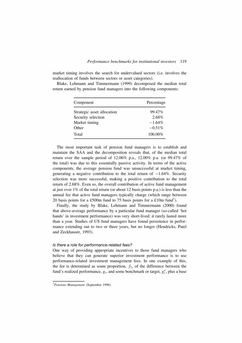
market timing involves the search for undervalued sectors (i.e. involves thereallocation of funds between sectors or asset categories).

Blake, Lehmann and Timmermann (1999) decomposed the median totalreturn earned by pension fund managers into the following components:

Component Percentage

Strategic asset allocation 99.47%Security selection 2.68%Market timing −1.64%Other −0.51%

Total 100.00%

The most important task of pension fund managers is to establish andmaintain the SAA and the decomposition reveals that, of the median totalreturn over the sample period of 12.06% p.a., 12.00% p.a. (or 99.47% ofthe total) was due to this essentially passive activity. In terms of the activecomponents, the average pension fund was unsuccessful at market timing,generating a negative contribution to the total return of −1.64%. Securityselection was more successful, making a positive contribution to the totalreturn of 2.68%. Even so, the overall contribution of active fund managementat just over 1% of the total return (or about 12 basis points p.a.) is less than theannual fee that active fund managers typically charge (which range between20 basis points for a £500m fund to 75 basis points for a £10m fund7).

Finally, the study by Blake, Lehmann and Timmermann (2000) foundthat above-average performance by a particular fund manager (so-called ‘hothands’ in investment performance) was very short-lived: it rarely lasted morethan a year. Studies of US fund managers have found persistence in perfor-mance extending out to two or three years, but no longer (Hendricks, Pateland Zeckhauser, 1993).

Is there a role for performance-related fees?One way of providing appropriate incentives to those fund managers whobelieve that they can generate superior investment performance is to useperformance-related investment management fees. In one example of this,the fee is determined as some proportion, f1, of the difference between thefund’s realized performance, gt , and some benchmark or target, g∗

t , plus a base

7Pensions Management (September 1998).


fee to cover the fund manager’s overhead costs, set as a fixed proportion, f2,of the absolute value of the fund (Vt in period t):

Performance-related fee in period t = f1(gt − g∗t )Vt + f2Vt (5.1)

This would reward good ex post performance and penalize poor ex postperformance, whatever promises about superior ex ante performance had beenmade by the fund manager. The fund would have to accept a reduced fee oreven pay back the client if gt was sufficiently below g∗

t (although the lattercase generally involves credits against future fees rather than cash refunds).

Another possibility that is less extreme since it does not involve refunds is:

Performance-related fee in period t = fiVt (5.2)

where fi is the fee rate if the fund manager’s return is in the ith quartile.An example of this second type of fee structure is that of the Newton

Managed Fund whose particular fee structure is listed in Table 5.1. Figure 5.2illustrates how this fee structure might work in practice. The chart shows thedistribution of fees payable to the manager of a middle-sized fund, basedon a Monte Carlo simulation. The 90% confidence interval for the fees liesbetween 0.22 and 0.45% p.a., while there is a 25% chance that the fee willexceed 0.37% p.a. and a similar chance that it will be less than 0.31% perannum. A mean annual charge of 0.34% implies a total take of approximately8.9% of the terminal fund value over an investment horizon of 25 years.

The level set for the target g∗t will have important implications for the

outcome. If the target is unrealistic and outside the range of performanceexpected by a skilled fund manager, the only way the manager can reason-ably achieve the stipulated performance is by increasing the volatility of hisinvestment strategy, i.e. by increasing risk. This is highly relevant in practiceas some targets are very hard to achieve. Examples of these are: ‘beat themedian fund by 2 percentage points over a three-year rolling period’, or ‘be

Table 5.1 Newton Managed Fund

Quartile rank Fund size

Up to £10m £10–£50m Above £50m

1st 0.94% 0.59 0.042nd 0.79 0.44 0.03Median 0.69 0.34 0.023rd 0.59 0.24 0.014th 0.44 0.09 0.01

Source: Newton Fund Managers.


0

1

2

3

4

5

6

7

8

Per

cent

ages

0.21

0.24

0.26

0.29

0.31

0.34

0.37

0.39

0.42

0.44

Per cent of fund value

Quartile rank Fee (%)

1st 0.592nd 0.44Median 0.343rd 0.244th 0.09

Note: The frequency diagram shows the annual distribution of performance-related feesin a fund with fees calculated according to the following performance scale:

The Monte Carlo simulation assumes the following: a fund with a 25-year investmenthorizon, a distribution of returns which is normal with a mean of 9% p.a. and a standarddeviation of 18%, and 1000 replications. Based on long-run returns reported in CreditSuisse First Boston's Equity-Gilt Study (2000), such a portfolio would be invested 35%in equities and 65% in bonds.

Figure 5.2 Frequency distribution of performance-related fees

in the upper quartile of performance’. There is an unconditional probability of75% of failing to achieve the second target! Clients/trustees are beginning toaccept that high targets will most likely be associated with greater volatility inperformance, unless the client has a priori information that the fund manageris genuinely capable of delivering the target performance.

Clients/trustees are also beginning to accept that targets based on thepeer-group median or peer-group distribution are very likely to distort fund


manager behaviour. This is partly because the median performance is really anoutcome rather than a target. Whereas a fund manager knows the compositionof an external index prior to making his own investments and so knows howmuch he is overweight or underweight in different securities, he will not knowfor sure what the asset allocation of the median fund manager is until the endof the performance period. All fund managers will be in the same position andthis provides a strong incentive for fund managers not to deviate too far fromeach other. Hence, we find that there is a tight distribution of fund managersaround the median fund manager who, in turn, generates a performance littledifferent from that of a passive index matcher. Those fund managers whobeat the median fund by 2 percentage points over a three-year rolling period,or who end up in the upper quartile of performance, are therefore more likelyto do so by chance than by skill.

All this suggests that the target g∗t should be set in relation to an external

benchmark rather than to a peer-group benchmark if clients/trustees wishtheir fund managers to pursue genuinely active fund management strate-gies. However, this makes quartile-based fee structures virtually impossible toimplement, since information on the distribution of returns around the medianvalue of the external index is not collected centrally.

It is particularly important for the fee rate to be symmetric about thetarget g∗

t , so that underperformance is penalized in exactly the same waythat outperformance is rewarded. The worst possible fee structure from theclient/trustee’s point of view would be one that rewarded outperformance butdid not penalize underperformance. An example of this would be:

Performance-related fee in period t = max[0, f1(gt − g∗t )Vt ] + f2Vt

(5.3)This particular fee structure would simply encourage the fund manager to takerisks with the client/trustee’s assets. If the fund manager’s risk taking paid off,he would receive a large fee. If, on the other hand, performance was disastrous,the fund manager would still get the base fee. All the risk of underperformance(at least in the short term) therefore falls on the client/trustee.

How frequently should fund managers be assessed?A final issue of importance concerns the frequency with which fund managersare assessed against the benchmark. Despite having very long-term investmentobjectives, the performance of pension fund managers is typically assessed ona quarterly basis. This is said to provide another disincentive from engagingin active fund management because of the fear of relative underperformanceagainst the peergroup and the consequent risk that an underperforming fundmanager will be replaced.


The frequency with which fund managers have their performance assessedought to be related to the speed with which market anomalies are corrected.Suppose, as argued above, the benchmark has been set in relation to the SAA.Then it is the fund manager’s performance in the two active strategies of stockselection and market timing that should be judged against the benchmarkprovided by the SAA. So the critical question is how long does it take forundervalued stocks to become correctly priced or for market timing bets tosucceed? If financial markets are relatively efficient, then pricing anomaliesshould be corrected relatively quickly. This appears to suggest that a relativelyshort evaluation horizon is appropriate. To illustrate using a somewhat extremeexample, if a market timing bet that involves, say, a significant underweightingof the US stock market, has not paid off after 10 years, then we might betempted to say that the bet was a bad one.

However, two points speak against the use of relatively short evaluationhorizons. The first has to do with time-variations in the investment opportu-nity set as represented by the relative expected returns and the conditionalvariances and covariances between the different asset classes. Many studiesin the finance literature suggest that the first and second moments of returnson different asset classes vary systematically as a function of the underlyingstate of the world. Nevertheless, there is considerable uncertainty about howbest to model such variations. But it seems reasonable to expect a successfulmarket timing strategy to be linked to the ability to anticipate changes in theunderlying economic state. This tends to evolve over fairly long periods oftime, as exemplified by the 10-year expansion in the US economy up to 2000.If clients want fund managers to time swings in the business cycle, a longevaluation horizon would seem more appropriate.

The second justification for using a longer investment horizon is that per-formance is measured with so much noise that it is in effect impossible toassess true fund management skills based on a short performance horizon.Under reasonable assumptions,8 it is possible to generate the following rela-tionship between the length of the performance record and the power of thetest for assessing fund management skills:

Power Required data record

25% 3.5 years50% 8 years90% 22 years

8See the Appendix.


0.00

0.10

0.20

0.30

0.40

0.50

0.60

0.70

0.80

0.90

1.00

0.1 3.5 6.9 10.3 13.8 17.2 20.6 24.0 27.4 30.8 34.3 37.7 41.1

Years

Source: See Appendix.

Pow

er

Figure 5.3 Power function – probability of correctly detecting abnormal performance

These figures are derived from Figure 5.3. The power of the test measuresthe probability of correctly rejecting the null hypothesis that the fund managergenerates no abnormal performance. It is clear from the figures that it takesa long time to detect with reasonable confidence that the performance of thefund manager is abnormal. And this result is dependent on an unchanginginvestment opportunity set which is in itself an unlikely eventuality over a22-year time horizon.

5.3 WHAT ARE THE ALTERNATIVES?

Recently, the academic literature has begun to investigate alternative bench-marks, based on extensions to the Capital Asset Pricing Model (CAPM).They help to identify the sources of any under- or outperformance by fundmanagers. There are also fixed benchmarks.

5.3.1 Single-index benchmarks with time-varying coefficients

The external benchmarks considered above are single-index benchmarks thatcan be justified by the CAPM, invented by Nobel prize winner Bill Sharpeand now one of the cornerstones of modern finance theory.

What is the CAPM?The CAPM decomposes the expected return on a fund into two parts. Thefirst is the return on a riskless asset such as Treasury bills: all professionalinvestors should be expected to generate a return exceeding that on Treasury


bills! The second is the additional return from taking on ‘market risk’. This,in turn, has two components: the ‘market risk premium’ (otherwise called the‘excess return on the market’ or the ‘market price of risk’), and the ‘quantity’of market risk assumed by a particular fund as measured by that fund’s ‘beta’.

The market risk premium is measured by the difference between theexpected return on the market index and the risk-free rate. The principalmarket index in the UK is the FTA All Share Index and many equity fundmanagers have this index as their single-index benchmark. The historicallong-run market risk premium for the UK is about 6% p.a.

The beta of a fund measures the degree of co-movement between the returnon the fund and the return on the market index. Technically the beta is cal-culated as the ratio of the covariance between the returns on the fund andthe market to the variance of the return on the market. It is also equal to theproduct of the standard deviation of the return on the fund and the correlationbetween the returns on the fund and the market. These are exactly the sameformulae as the slope or beta coefficient in a time-series regression of theexcess return on the fund on an intercept and the market risk premium, whichexplains how a beta coefficient is so named. If the standard deviation of thereturn on the fund or the correlation between the returns on the fund and themarket are high, then the fund’s beta will be high. The beta of the marketindex itself is unity. If the fund beta exceeds unity, the fund is more volatilethan the market: a beta of 1.1 implies that the fund is 10% more volatile thanthe market so that if the market rises or falls by 20%, the fund will rise orfall by 22%.

The CAPM can be expressed as follows:

Excess return on fund = Alpha + Beta of fund × Market risk premium= Alpha + Market risk of fund (5.4)

where the excess return on the fund is the difference between the realizedreturn on the fund and the risk-free rate. The CAPM is illustrated in Figure 5.4.

If the excess return on the fund exceeds the market risk of the fund, thenthe fund has generated an above-average performance. The difference betweenthe excess return on the fund and the market risk of the fund is called thefund ‘alpha’ (sometimes it is called the ‘Jensen alpha’ after its inventor). Asuccessful fund manager therefore generates a positive alpha. However, it isimportant to recognize that a fund return exceeding the market index returndoes not necessarily imply a positive alpha. It is possible for a fund to takeon a lot of market (i.e. beta) risk and generate a return higher than the marketindex return, but nevertheless generate a negative alpha: this would indicatethat the market risk assumed by the fund manager was not fully rewarded.


Beta (A)

Source : Blake (2000: Fig.14.8); Note: M, excess return on the market index (which has abeta of unity), A − positive excess return of fund A, B − negative excess return of fund B.

1 Beta (B) Beta of fund

Mar

ket r

isk

prem

ium

Exc

ess

retu

rn o

n fu

nd

A

Alp

ha (

A)

Mar

ket r

isk

(A)

M

B

Alp

ha(B

)

Figure 5.4 The Capital Asset Pricing Model

This is the case for fund manager B in Figure 5.4: although B generateda return above that of both the market and fund manager A, A is a moresuccessful fund manager.

How has the CAPM been extended?This is how a single-index benchmark with constant coefficients for alphaand beta operates within the context of the CAPM. A recent developmenthas been to make the beta coefficient of the CAPM time-varying, that is toallow for predictable time-variation in the beta coefficient on the grounds thatfund managers should not be credited with using publicly available informa-tion concerning changes in investment opportunity sets when making theirinvestment decisions (see Ferson and Schadt (1996); even more recently,Christopherson, Ferson and Glassman (1998) have extended this procedure toallow for time-varying alpha coefficients).

The beta coefficient is made a linear function of a set of predeterminedvariables: the lagged values of the short-term yield on T-bills, the long-termyield on government bonds and the dividend yield on an equity index such


as the FTA All Share Index; these are all standard regressors with a longtradition in the literature on the predictability of stock returns. So the betacoefficient in this case is determined as follows:

Beta of fund = B(0) + B(1) × T -bill yield lagged+ B(2) × Government bond yield lagged+ B(3) × Dividend yield lagged (5.5)

When Blake and Timmermann (1998) substituted this beta equation into theCAPM equation above and applied it to UK unit trusts over the period1972–1995, they found it raised the estimate of alpha for the UK balancedsector from −0.74 to −0.52. In other words it lowered the estimate of under-performance slightly for that sector. It made little difference to other sectors,however.

5.3.2 Multiple-index benchmarks

Another recent innovation has been the use of multiple-index benchmarks.For example, Elton et al. (1993) pioneered the use of a ‘four-index’ bench-mark consisting of the excess return on large-cap stocks (i.e. a large-cap riskpremium), the excess return on small-cap stocks (i.e. the small-cap risk pre-mium), the difference between the returns on an equity growth index and anequity income index (i.e. a growth minus income factor) and the excess returnon bonds (i.e. a bond risk premium). The multiple-index CAPM thereforebecomes:

Excess return on fund = Alpha + Beta (1) × Large-cap risk premium+ Beta(2) × Small-cap risk premium+ Beta(3) × (Growth−Income)+ Beta(4) × Bond risk premium (5.6)

Again, a successful fund manager will generate a positive alpha after tak-ing into account these four factors. In other words, a successful active fundmanager will be one who does more than simply buy a portfolio of large-capstocks, small-cap stocks, growth stocks and corporate bonds.

A variation on this model has been applied to UK unit trusts by Blake andTimmermann (1998). For the UK Equity General sector, for example, theyfound the following three-index model for the sample period 1972–1995:

Excess return on fund = −0.16 + 0.86 × Market risk premium+ 0.33 × Small-cap risk premium− 0.07 × Bond risk premium (5.7)


This indicates that after taking into account market risk, small-cap risk andbond risk, a typical unit trust from the UK Equity General sector generateda negative alpha (i.e. underperformed on a risk-adjusted basis) by 16 basispoints p.a. on average.

The wider use of multiple-index benchmarks which include small-cap andmicro-cap indices might well help to encourage institutional investors to con-sider their investments in these sectors more carefully since they would nowhave a specific reference point in the form of a performance benchmark.

5.3.3 Fixed benchmarks

Another possibility is to use a fixed benchmark. This in a sense is what wasimplied by the long-term financial assumptions of the MFR9:

• Rate of inflation – 4% p.a.• Effective rate of return on gilts – 8% p.a.• Effective rate of return on equities – pre-MFR pension age – 9% p.a.• Effective rate of return on equities – post-MFR pension age – 10% p.a.• Rate of increase of GMP under Limited Revaluation – 5% p.a.• Rate of statutory revaluation for deferred benefits – 4% p.a.• Rate of LPI increase in payment – 3.5% p.a.• Rate of increase in post-1988 GMPs – 2.75% p.a.• Rate of increase in S148 Orders – 6% p.a.• The real rate of return on index – linked stocks is I where (1 + I ) =

1.08/1.04.

The problem with fixed benchmarks is their arbitrary nature. Even if they arebased on historical experience, there is no guarantee that they would provideaccurate forecasts for the future. For example, the extraordinary performanceof the UK stock market over the last quarter century has generated an equityrisk premium approaching 10%. It would be highly inappropriate to use thisfigure to set a benchmark for equities over the next 25 years.

5.4 BENCHMARKS BASED ON LIABILITIES

5.4.1 Liability benchmarks

What are the key liability benchmarks?The benchmarks considered so far, appropriately adjusted for the relevantuniverse, are suitable for any institutional investor without matching liabilities,

9See ‘Current Factors for Use in MFR Valuation’ in Guidance Note 27 of the Faculty and Instituteof Actuaries, 1998, B27.11–12.


such as a defined contribution pension fund or a unit or investment trust. Theyare also used in practice by defined benefit pension funds which do havematching liabilities. However, it is important to consider explicit liability-based benchmarks. For example, the liabilities of a final salary pension plandepend on expected earnings growth; they also depend on other factors suchas forecasts of life expectancy and the discount rate used for discountingliabilities.

One natural benchmark would therefore be earnings growth. A relatedbenchmark might be GDP growth. Earnings growth and GDP growth arerelated in the long run, since the share of wages in national income does nottrend significantly over time: in fact in long-run dynamic equilibrium, earningsgrowth and GDP growth will be the same. However, over the course of anybusiness cycle, the growth rates in these two variables can differ substantially.

Another natural benchmark for pension funds would be the growth ratein consumption expenditure, since a pension plan’s purpose is to financeconsumption expenditure in retirement. Strictly speaking the weights for theconsumption expenditure index should reflect the pattern of expenditure bythe elderly, which might have a higher weight in medical expenses and alower weight in foreign holidays, say, than younger more active cohorts ofthe population. Again in long-run dynamic equilibrium, the growth rates inGDP and consumption expenditure will be the same (otherwise the savingsratio will tend towards either zero or unity).

Why are they easy to beat?A benchmark based on the growth rate of liabilities would be a fairly easy oneto beat, since the returns on funds with a substantial weighting in equities tendto exceed the growth rate of liabilities whether measured by earnings growth,GDP growth or consumption growth. There is a good technical reason whythis should be the case: it has to do with what is known as the ‘dynamicefficiency’ of the economy.10

It is possible for economies to accumulate too much productive capital (thatis, the plant equipment and machinery used by workers to produce the goodsand services that consumers wish to buy). As more capital is accumulated, itsreturn falls: this is because the additional capital is being applied to increas-ingly marginal and less productive investment opportunities. When there istoo much capital, the return falls below the growth rate of the economy. Whenthis happens, the economy is said to be ‘dynamically inefficient’: everyone inthe economy would be better off if there was less saving and investment andmore consumption. With less investment, the capital stock falls (as depreciated

10See, e.g., Blanchard and Fischer (1989).


capital is not replaced) and the return on capital rises above the growth rateof the economy as measured by the GDP growth rate. When this happens,the economy is in a state of dynamic efficiency.

Most of the key economies in the world have been assessed as being dynam-ically efficient.11 This means that, in such economies, the returns on financialassets such as equities (which represent claims on the capital stock) will onaverage exceed the growth rate of GDP, even though there will inevitably besome years when this does not happen. So a passive strategy of holding abroadly based equity portfolio will generate a return that is likely to exceedwage growth, GDP growth or consumption expenditure growth in most years.

How should future liabilities be discounted?The discount rate for discounting future liabilities provides another possiblebenchmark if it is set independently of the return on the assets in the fund.Some asset-liability models use the weighted-average return on the assets inthe fund as the discount rate for liabilities: obviously this could not be usedas a benchmark. Others use the yield on long-term government or corporatebonds.

The 1995 Pensions Act’s MFR norms, for example, used government bondyields to determine the present value of pensions in payment12:

The current gilt yields to be used for valuing pensioner liabilities should bethe gross redemption yield on the FT-Actuaries Fixed Interest 15 year MediumCoupon Index or the FT-Actuaries Index-linked Over 5 years (5% inflation)Index, as appropriate. In the case of LPI pension increases, either fixed-interestgilts with 5% pension increases or index-linked gilts with a 0.5% addition tothe gross redemption yield should be used, whichever gives the lower valueof liabilities. Similar principles should be applied for other pensions which areindex-linked but subject to a cap other than 5%.

The justification for using a bond yield is that pensions-in-payment liabilitiesare less risky than equities and hence should be discounted at a lower yield.On the other hand, pensions-in-payment liabilities are not risk free, and sothe discount rate should be higher than that on Treasury bills. This suggeststhat a bond yield provides an appropriate discount rate. The Faculty andInstitute of Actuaries chose the above government bond yields to calculatepensions-in-payment liabilities under the MFR.13

11See Abel et al. (1989).12See ‘Current Factors for Use in MFR Valuation’ in Guidance Note 27 of the Faculty and Instituteof Actuaries, 1998, B27.11–12.13The MFR allowed the accruing liabilities of active workers to be discounting using a weightedaverage of long-run gilt and equity yields, with the weights reflecting the asset mix in the fund.


However, for financial reporting purposes, the Accounting Standards Boardrequires, in FRS17, that all pension liabilities (including those relating to theaccumulating liabilities of active members as well as pensions in payment)are valued using an AA corporate bond yield.14

Whichever particular bond yield is used, a fund with a heavy equity com-ponent is likely to beat a benchmark based on either government or corporatebond yields in most years, on account of the sizeable positive equity riskpremium in the UK financial markets. On the other hand, since equity valuesare more volatile than those of bonds, there will also be a greater chance ofproducing periodic deficits in the fund.

Explicit liability benchmarking, although currently not very common, willsoon become so for a number of reasons. First, there is the increasing maturityof pension funds: the crystallization of liabilities in terms of a specific streamof pensions-in-payment will inevitably move pension fund asset holdingstowards bonds as the natural matching asset. Second, the financial reportingdevelopments just mentioned will introduce a common liability benchmarkfor all schemes. Third, the replacement of the MFR with a scheme-specificfunding standard, as announced by the government in March 2001 and rec-ommended by the Myners Review (2001), will lead to the introduction ofscheme-specific liability benchmarks.

5.4.2 Measuring the performance of pension funds using liability-drivenperformance attribution

‘Liability-driven performance attribution’ (LDPA) is the name given to theframework for analysing performance measurement and attribution in the caseof asset-liability managed (ALM) portfolios, that is, portfolios whose invest-ment strategy is driven by the nature of the investing client’s liabilities.15

We can illustrate the LDPA framework using the following balance sheetfor an asset-liability managed pension fund16:

Assets Liabilities

Liability-driven assets A Pension liabilities L

General assets E Surplus S

14This was the same yield chosen by the equivalent US accounting standard, FAS87.15See Plantinga and van der Meer (1995).16The components of the balance sheet are measured in present value terms. Also for simplicityof exposition, we assume that L relates to accrued past service; thus future contributions areexcluded from the balance sheet: actuaries call this the ‘accrued benefits method’ of valuingpension liabilities.


Suppose that the ‘pension liabilities’ (L) generate a predetermined set offuture cash outflows. The fund manager can meet these cash outflows byinvesting in fixed-interest bonds (A) with the same pattern of cash flows;these bonds constitute the ‘liability-driven assets’ (LDAs) in the balance sheetabove.17 Suppose that the pension fund ‘surplus’ (S) is invested in ‘generalassets’ (E). These can be any assets matching the risk-return preferencesexpressed by the pension scheme’s sponsor (e.g. equities). The surplus isdefined as assets (A+ E)minus liabilities (L).18 The return on the surplus isdefined as:

rSS = rEE + rAA− rLL (5.8)

where:rS = the rate of return on the surplusrE = the rate of return on the general assetsrA = the rate of return on the liability-driven assetsrL = the payout rate on the liabilities.

Both the pension liabilities and the liability-driven assets will be sensitive tochanges in interest rates. Higher interest rates reduce the present value of pen-sion liabilities. Similarly, higher interest rates reduce the value of fixed-interestbonds, since a given stream of fixed-coupon payments is worth less todaywhen yields on alternative assets are higher.19

Assuming that interest rate risk is the only source of risk to this portfolio,we can use equation (5.8) to derive a decomposition of portfolio performanceas follows. First, we rewrite the return on the general assets as:

rEE = rES + rE(E − S) (5.9)

and the return on the liability-driven assets as:

rAA = rAL+ rA(A− L) (5.10)

17If the pension liabilities are indexed to uncertain real wage growth or to future inflation thenthe liability-driven assets will be the assets most likely to match the growth rate in earnings or ininflation over the long term (e.g. indexed bonds, equities and property). But to keep the analysissimple, we assume that the cash flows on future pension payments are known.18Following the 1986 Finance Act, the surplus in UK pension funds cannot exceed 5% of the valueof the liabilities. Following the 1995 Pensions Act, the deficit in pension funds cannot exceed 10%of the value of the liabilities and must be reduced to zero within a maximum of ten years.19It is theoretically possible to structure the liability-driven assets in such a way that the pensionfund is immunized against interest rate movements. When this happens, the surplus will not respondto interest rate movements. Immunization is explained in Blake (2000: Chap. 14).


Then we can divide each side of (5.8) by S and substitute (5.9) and (5.10) toget the LDPA20:

rs = rES + rE(E − S)

S+ rAL+ rA(A− L)

S− rL

L

S

= rE + λ(rA − rL)+ γ (rE − rA)

= rE + λ(rA − rA)+ λ(rA − rL)+ γ (rE − rA) (5.11)

or:

Rate of return on the surplus = Rate of return on the general assets+ Rate of return on the LDAs due to

security selection+ Rate of return on the LDAs due to

market timing+ Rate of return from a funding

mismatch

where:

λ = L

S= financial leverage ratio

γ = L− A

S= E − S

S= funding mismatch ratio

rA = the expected return on bonds when they are correctly pricedon the basis of the spot yield curve (i.e. when the futurecoupon payments are discounted using the appropriate spotyields) (see, e.g., Blake (2000: Chap. 5)).

The four-component LDPA in (5.11) can be explained as follows:

1. The rate of return on general assets (rE). This can be analysed usingstandard techniques, e.g. comparing performance against a pre-agreed peer-group or external benchmark, as outlined in sections 5.2 and 5.3 above.

2. The rate of return on the liability-driven assets due to stock selection interms of, say, credit quality management or sector management. This fol-lows because rA is the actual return generated by the bonds chosen bythe fund manager, whereas rA is the benchmark return on the bonds if

20In the case where the surplus is exactly zero, the decomposition in (5.11) is not defined. Thefund manager has just generated a sufficient return to meet the payout rate on liabilities. The LDPAin this case would be based on rL = rE(E/L)+ rA(A/L) where (E/L) is the portfolio weight ingeneral assets and (A/L) is the portfolio weight in liability-driven assets (see (5.8)).


they were correctly priced according to the spot yield curve: (rA − rA) istherefore the excess return arising from the stock selection skills of thefund manager.

3. The rate of return on the liability-driven assets due to market timing, thatis, from choosing a portfolio of bonds with a maturity structure that differsfrom that of the underlying liabilities, thereby deliberately leaving theportfolio partially exposed to interest rate risk.

4. The rate of return from a funding mismatch, that is, from active manage-ment of the liability-driven assets such that part of this category is investedin riskier general assets such as equities.

We can illustrate the LDPA using an example. Suppose that a pension fundhas the following balance sheet at the start and end of the year:

Assets LiabilitiesStart End Start Endyear year year year

Liability-driven Pensionassets (A) 900 997 liabilities (L) 1,000 1,107

General assets (E) 150 169 Surplus (S) 50 59

1,050 1,166 1,050 1,166

We will assume that the liability-driven assets are bonds, while the generalassets are equities (and that equities have no yield curve effect). The valueof the liabilities is calculated as the present value of the liability cash flowsusing appropriate spot yields as discount rates. We have the following returnson the components of the balance sheet:

Component Actual rate Benchmark rateof return (%) of return (%)

Bonds rA = 10.78 rA = 10.66 (assumption)Equities rE = 12.67 rE = 13.30 (assumption)Liabilities rL = 10.70

The actual rates of return are found by taking the difference between theend-of-year and start-of-year values as a ratio of the start-of-year values. Thebenchmark return on bonds is calculated in a similar way but based on start-and end-year present values of coupon payments using appropriate spot yields.The benchmark return on equities is simply the realized return on a relevantindex, e.g. the FTA All Share Index.


Using equation (5.11) with λ = L/S = 20 and γ = (L− A)/S = 2 (usingstart-of-year values), the LDPA is determined as follows:

Component Return (%)

1. General assets (rE) 12.672. Security selection (λ(rA − rA)) +2.403. Market timing (λ(rA − rL)) −0.804. Funding mismatch (γ (rE − rA)) +3.78

Total 18.05%

The total rate of return on the surplus of 18.05% is made up of 12.67%from the performance of the general assets, 2.40% from successful stockselection of the bond portfolio, 3.78% from a successful funding mismatch,and a loss of 0.80% from market timing. The security selection and markettiming effects are magnified by a high leverage ratio (λ) of 20 (the minimumthat is permissible since the surplus may not (in the long term) exceed 5%of liabilities), while the funding mismatch effect is magnified by a smallerfunding mismatch ratio (γ ) of 2. The positive net return of 1.60% fromactive fund management (i.e. the sum of the returns from security selectionand market timing) and the positive net return from a funding mismatch helpto generate a high surplus return. However, this cannot conceal the fact thatthe fund manager underperformed the benchmark in terms of general assetsby 0.63%.

The LDPA therefore tells us a great deal about the investment skills of thepension fund manager when he or she is constrained on the liability side ofthe balance sheet. The only additional information that is required over thecurrent performance measurement framework is as follows: the present valueof the pension liabilities (as determined by the pension scheme’s actuary),together with the payout rate on these, and the value of the liability-drivenassets, together with a customized benchmark return on these.

5.5 WHAT HAPPENS IN OTHER COUNTRIES?

5.5.1 USA

Benchmarking is usually done on an asset class basis against well-known totalreturn indexes. Thus the performance of domestic equity managers is assessedrelative to the S&P 500 total return index, fixed-income managers relative tothe Lehman aggregate, etc. The other kind of benchmarking is relative to the


average within a peer group. Thus the average of all equity managers whosubscribe to Lipper’s performance service becomes the benchmark for all themanagers in that ‘universe’.

5.5.2 Japan

No definite benchmarks have been established yet in Japan. Tentatively, theannual rate of return from the Treasury bond (with a maturity in excess of10 years) plus 0.1% is used, which is just equivalent to the investment per-formance from the Fiscal Investment and Loan Program.

5.5.3 Germany

There are four different pension vehicles in Germany.

(1) Direct commitments (book reserves)Since there are no separate funds, there is no investment choice. Fifty-sevenper cent of total occupational pension liabilities in Germany are financedthrough direct commitments.

(2) Support fundsThere are no portfolio restrictions for support funds whatsoever. Instead,investment decisions are made solely by the employer. Therefore, there iseither no communicated benchmark at all, or the employer selects the bench-mark on a discretionary basis. There are more than 5,000 support funds inGermany but they account for only 8% of total pension assets.

(3) Direct insuranceCurrently, the benchmark is 4% p.a. However, there is a public debate aboutwhether this is too high since interest rates are currently low. Therefore,the government is considering lowering the benchmark to 3.5%. There arenumerous direct insurance contracts in Germany and they account for 12%of total pension assets.

(4) Pension fundsPension funds are the only vehicle where having a proper benchmark wouldmake sense. However, pension funds are not required to make detailed infor-mation about their investment returns, etc. publicly available. This kind ofinformation need only be disclosed to the regulator. Currently, there are180 pension funds in Germany and they account for 22% of total pensionassets.


5.5.4 Italy

Mixes of well-known indices like JPM bond and MSCI stocks in varyingproportions. The exact benchmark of each pension fund is not made public.While it can be requested from the fund, this is a long process.

5.5.5 Chile

The benchmark is the average of the return of the other pension funds (AFPs).The use of market indices has been rejected because the local market bench-marks are of questionable applicability. Pension funds are subject to a numberof investment constraints, not taken into account in the existing benchmark,e.g. the weights in the benchmark are changed every quarter but the pensionfunds invest with a very long horizon.

5.6 CONCLUSION

Performance benchmarks are important for three key reasons: they help tomeasure the investment performance of institutional fund managers, they pro-vide clients/trustees with a reference point for monitoring that performanceand they can also have the effect of modifying the behaviour of fund man-agers. But benchmarks are not the only factor of importance: fee structuresalso have a major impact.

At the same time, there needs to be a much greater understanding byclients/trustees of the nature of active fund management. At its simplest,an active portfolio can be interpreted as a passive portfolio plus a set ofactive side bets against the market. The passive component of the portfoliois the strategic asset allocation and, if the benchmark is set appropriately, theperformance of the SAA should exactly match the benchmark. The activecomponents should beat the benchmark if the fund manager’s side bets aresuccessful and it should be possible to assess this fairly quickly if financialmarkets are relatively efficient.21

A good benchmark combined with a suitable fee structure would there-fore enable an above-average fund manager to deliver, on a systematic basis,superior investment performance without taking on excessive risks. The factthat the evidence indicates that fund managers cannot systematically deliversuperior investment performance over extended periods is more an indicationof the efficiency of financial markets than of the ineffectiveness of either thebenchmark or the particular fee structure.

21Although we also showed that the noise generated by changing investment opportunity sets canmake it difficult to assess genuine fund management skill over short horizons.


In addition, a good benchmark would be one that did not have built-inbiases either in favour of or against particular asset classes. In particular, adynamic financial system demands that there is no bias against start-up capital,and so a good benchmark would contain the appropriate market weightingin venture capital securities. A good benchmark might therefore be basedon a multiple of indices that covers all the key asset categories as well asliabilities. In turn, a good fee structure has an appropriate performance-relatedelement.

There are, of course, unsuitable benchmarks and fee structures. Peer-groupbenchmarks provide a strong incentive not to underperform the median fundmanager, while fee structures based on the value of assets under managementdo not provide a particularly strong incentive to engage seriously in activefund management. We should not be surprised to find that the outcome isherding around the median fund manager who, in turn, is doing little morethan match the index. In other words, this benchmark and fee structure havethe effect of modifying the behaviour of the fund manager from that whichwas agreed with the client/trustee. This is rational behaviour by the fundmanager since his long-term survival in the industry depends on his rela-tive performance against other fund managers. But it is certainly not whatthe client/trustee intended. Similarly, a fee structure that awarded outperfor-mance of a benchmark without penalizing underperformance would lead tothe fund manager taking risks with the client/trustee’s assets in a way that theclient/trustee did not intend. As a final example, the maturing of net investorssuch as pension funds suggests that scheme-specific benchmarks that reflectthe maturity of a particular scheme’s liabilities become increasingly appropri-ate, while, correspondingly, those based on external or peer-group benchmarksbecome less so.

Benchmarks are important, but so are fee structures. They can either providethe right incentives for fund managers or they can seriously distort theirinvestment behaviour.

5.7 APPENDIX: DERIVING THE POWER FUNCTION

Suppose a fund’s monthly excess returns are generated by the equation:

Rt = α + βRmt + εt , εt ∼ N(0, σ 2)

where Rt is the excess return on the fund in period t , over and above therisk-free rate of return, β is its beta, Rmt is the excess return on the marketportfolio in period t , εt is the residual in period t and α measures the fund’sgenuine ability to outperform. How long will it take for the trustees to detect


with reasonable statistical reliability whether the fund produces abnormal per-formance? To answer this question, suppose that α = −0.1 and it is knownthat β = 1 and σ = 0.5. For continuously compounded monthly returns datathese parameter values correspond to a fund that underperforms the index by1.2% per year while the idiosyncratic risk is 6% per year. Assuming that thesize of the statistical test for the fund manager’s ability to add value, p, is thestandard 5%, we can illustrate the difficulty of conducting statistical inferenceabout management skills by calculating the power function for a test of thenull hypothesis:

H0(no abnormal performance): α = 0

against the alternative hypothesis:

H1(abnormal performance): α = 0

We do so by computing how many months of data are needed to ensurea 10, 25 or 50% probability of correctly identifying the fund’s abnormalperformance. The null hypothesis is rejected if:

|Z| ≡∣∣∣∣ α − α0

σ/√n

∣∣∣∣ > z1−p/2

where α = ∑nt=1 (Rt − Rmt )/n is the estimated mean performance and α0 is

the value of α under the null hypothesis of zero abnormal performance. z1−p/2is the (1 − p/2) quantile of the distribution of the performance test statistic.The null is rejected if:

α < α0 − z1−p/2σ/√n

or

α > α0 + z1−p/2σ/√n

Otherwise it is accepted. Suppose that, under the alternative hypothesis, thefund manager’s performance is α1, so that α ∼ N(α1, σ/

√n). Then the rejec-

tion probability can be computed from:

P(α < α0 − z1−p/2σ/√n) = P

(α − α1

σ/√n<α0 − α1 − z1−p/2σ/

√n

σ/√n

)

= P

(Z <

α0 − α1

σ/√n

− z1−p/2)

= &

(α0 − α1

σ/√n

− z1−p/2)


where &(·) is the cumulative density function for a standard normal variate.Likewise, by symmetry of the normal distribution,

P(α > α0 + z1−p/2σ/√n) = P

(Z >

α0 − α1

σ/√n

+ z1−p/2)

= &

(α1 − α0

σ/√n

+ z1−p/2)

For example, if p = 0.05 so that z1−p/2 = 1.96 and α0 = α1 = 0, thenP(Z < −2) = P(Z > 2) = 0.025, so that the power of the test equals thesize of the test at 5%.

However, if α0 = 0, α1 = −0.1, σ = 0.5, we get the following relationbetween power (the probability of correctly rejecting the null) and sam-ple size:

P(Reject H0|α1, α0, σ, n) = Power(α1, α0, σ, n)

= &

(α0 − α1

σ/√n

− z1−p/2)

+&

(α1 − α0

σ/√n

+ z1−p/2)

= P(Z < −1.96 + 0.2√n)

+ P(Z < −1.96 − 0.2√n)

This relationship is used to calculate the results in the main text.

REFERENCES

Abel, A., Mankiw, N.G., Summers, L. and Richard, J. (1989) Assessing dynamic effi-ciency, Review of Economic Studies, 56, 1–19.

Benjamin, B., Haberman, S., Helowicz, G., Kaye, G. and Wilkie, D. (1987) Pensions:The Problems of Today and Tomorrow , Allen and Unwin, London.

Blake, D. (2000) Financial Market Analysis , Wiley, Chichester (especially, Chapters 5,13 and 14).

Blake, D. and Timmermann, A. (1998) Mutual fund performance: evidence from theUK, European Finance Review , 2, 57–77.

Blake, D., Lehmann, B. and Timmermann, A. (1999) Asset allocation dynamics andpension fund performance, Journal of Business, 72, 429–461.

Blake, D., Lehmann, B. and Timmermann, A. (2000) Performance Clustering andIncentives in the UK Pension Fund Industry , Pensions Institute, London, June(www.pensions-institute.org).

Blanchard, O.J. and Fischer, S. (1989) Lectures on Macroeconomics , MIT Press, Cam-bridge, MA.


Christopherson, J., Ferson, W. and Glassman, D. (1998) Conditioning manager alphason economic information, Review of Financial Studies, 11, 111–142.

Coggin, T.D., Fabozzi, F.J. and Rahman, S. (1993) The investment performance of USequity pension fund managers: an empirical investigation, Journal of Finance, 48,1039–1055.

Elton, E., Gruber, M., Das, S. and Hlavka, M. (1993) Efficiency with costly information:a reinterpretation of evidence from managed portfolios, Review of Financial Studies ,6, 1–22.

Ferson, W. and Schadt, R. (1996) Measuring fund strategy and performance in changingeconomic conditions, Journal of Finance, 51, 425–462.

Hendricks, D., Patel, J. and Zeckhauser, R. (1993) Hot hands in mutual funds: short-runpersistence of relative performance, Journal of Finance, 48, 93–130.

Lakonishok, J., Shleifer, A. and Vishny, R.W. (1992) The structure and performance ofthe money management industry, Brookings Papers: Microeconomics , 339–391.

Myners, P. (2001) Institutional Investment in the United Kingdom: A Review , HM Trea-sury, London, March.

Plantinga, A. and van der Meer, R. (1995) Liability-driven performance attribution,Geneva Papers on Risk and Insurance, 20, 16–29.

Timmermann, A. and Blake, D. (2000) Determinants of International Portfolio Perfor-mance, Pensions Institute, London, September (www.pensions-institute.org).

Wilson, Rt Hon. Sir H. (chairman) (1980) Report of the Committee to Review the Func-tioning of Financial Institutions , Cmnd. 7937, HMSO, London, June.

Documents

Chapter 5econweb.ucsd.edu/~atimmerm/benchmark.pdf · Chapter 5 Performance ... is much more prevalent with pension funds and mutual funds than with life funds. ... companies) that