Comparing means of 3 or more groups requires the use of different statistical tool, call1

the F-ratio. That tool is introduced in a later chapter.

107

CHAPTER 9

T-TESTS: EXAMINING DIFFERENCES BETWEEN MEANS

The previous chapter emphasized the importance of hypothesis testing within the context of

statistical research, but did not provide information about the specific research tools or statistics that

are employed in the process of hypothesis testing. Researchers have developed a variety of these

tools. The specific research tool examined in this chapter is the T-test. This statistic is used when a

researcher wishes to compare the means of two sample groups to test hypotheses related to the means

of the two overall populations represented by these samples. This chapter explains the theoretical1

foundations of the T-test and provides instruction in its use in the process of testing hypotheses.

The first step in the explanation of the t-test requires the introduction of a new concept. This

concept is a special form of sampling distribution referred to as the sampling distribution of mean

differences. The sampling distribution of mean differences is similar in function and importance to

the concept of the sampling distribution of means introduced in Chapter 7. Both are expected to

approximate the normal curve and are useful in provide a means of constructing confidence intervals

using the rules of probability. The sampling distribution of mean differences represents a theoretical

construct that represents the distribution of values that would be produced if a researcher drew

repeated samples from two groups and calculated the differences between each pair of sample means.

To illustrate, assume that a researcher selected 1000 samples of 100 teachers from region A and 1000

samples of 100 teachers from region B and calculated the salaries for each teacher. Each time the

researcher selected a sample from regions A and B, means were obtained for each sample. The

108

difference between the two means was calculated for each sample pair. These mean differences

could then be used to construct a frequency polygon called the sampling distribution of mean

differences. This distribution should closely approximate the normal curve shown in Figure 9:1.

FIGURE 8:1

SAMPLING DISTRIBUTION OF MEAN DIFFERENCE

The null hypothesis begins with the presumption that there is not a statistically significant

difference between groups. Since our research tools are based on testing this presumption, the mean

of a sampling distribution of mean differences is expected to be zero because the positive and

negative mean differences in a distribution tend to cancel each other out. For every negative

difference in means observed among samples drawn from equivalent populations, there tends to be a

positive value an equal distance from the mean observed between another pair of samples. Within the

sampling distribution of differences, most of the sample mean differences in the distribution fall close

to zero. There will be relatively few mean differences having an extreme value in either direction

from the mean. This important characteristic makes the sampling distribution of mean differences a

very useful tool in testing hypotheses.

109

As with the sampling distribution of means, knowledge of the mean and the standard

deviation of a distribution of mean differences is rarely, if ever, available. It would be a major effort

to select a large number of sample pairs in order to calculate a standard deviation for a distribution of

mean differences; however, this standard deviation plays an important role in testing hypotheses

related to mean differences. Fortunately, there is a simple method whereby the standard deviation of

the distribution of differences can be accurately estimated. On the basis of two samples actually

drawn, the estimate of the standard deviation of a sampling distribution of differences is called the

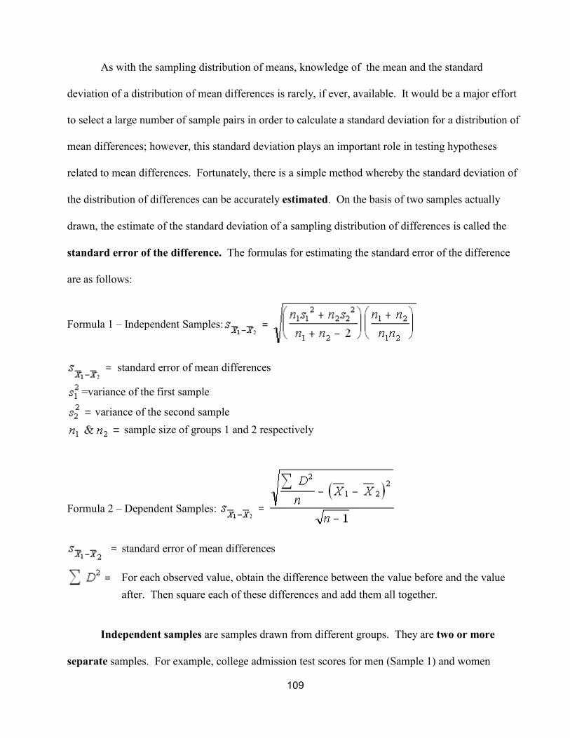
standard error of the difference. The formulas for estimating the standard error of the difference

are as follows:

Formula 1 – Independent Samples:

standard error of mean differences

=variance of the first sample

variance of the second sample

sample size of groups 1 and 2 respectively

Formula 2 – Dependent Samples:

standard error of mean differences

For each observed value, obtain the difference between the value before and the value

after. Then square each of these differences and add them all together.

Independent samples are samples drawn from different groups. They are two or more

separate samples. For example, college admission test scores for men (Sample 1) and women

W hen the number of degrees of freedom exceeds 30, t-distributions become almost2

indistinguishable from the normal curve. For that reason, the same critical value will be used with all tests

that involve more than 30 degrees of freedom.

110

(Sample 2) would be two independent samples. Individuals in independent samples must be included

in one and only one group. Dependent samples are those which are involve individuals or

phenomena observed at two different points in time. For example, student scores on their first and

second semester exams are dependent samples. In this example, two sets of data are used for the

same group of individuals or sample.

The second step in the process of testing hypotheses involves the computation of a t-statistic.

The t-statistic is used in a similar way to the z-scores discussed earlier in the text. It converts the

difference in means observed between the two sample groups under examination to units based on the

standard error of the mean differences. The formula for the t-statistic used in this process is:

Calculating a value for the t-statistic allows the researcher to test the validity of the null hypothesis

that has been proposed. Appendix D contains a table that provides the critical values for t at various

degrees of freedom. Critical values represent the positive and negative points in the distribution that2

mark the top and bottom end of a confidence interval for the standard error of mean differences in a

particular circumstance. For example, the critical value for t at the 95% level of confidence for a

sample with 5 degrees of freedom would be 2.571. This means that if the null hypothesis is true (the

true difference in the population means = 0) the laws of probability suggest that 95% of the time a

111

researcher should obtain a mean difference that was between -2.571 standard errors of the mean

difference and +2.571 standard errors of the mean difference. Once the critical values have been

obtained, they are compared to the calculated value of t. If the value of t falls outside of the range of

values marked by the positive and negative scores provided in Appendix D (-2.571 and +2.571 in our

example), the null hypothesis is rejected and the researcher must conclude that the difference in the

population means is NOT zero. If, however, the calculated value of t falls within the range of values

marked by the critical value provided in the appendix, the null hypothesis is accepted and the

researcher must conclude that there is not a statistically significant difference in the means of the two

populations.

At this point, it is useful to explain the rationale behind accepting the null hypothesis in the

above example. The null hypothesis is rejected if the probability is very small ( P = .05 or only 5

chances out of 100 ) that the obtained sample difference is a product of sampling error. At .05 the

null hypothesis is rejected if an obtained sample difference occurs by chance only 5 times out of 100.

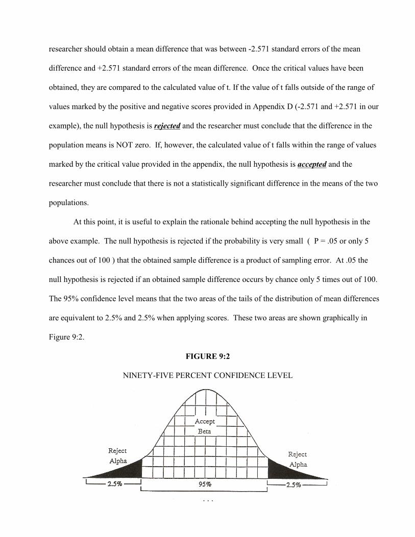
The 95% confidence level means that the two areas of the tails of the distribution of mean differences

are equivalent to 2.5% and 2.5% when applying scores. These two areas are shown graphically in

Figure 9:2.

FIGURE 9:2

NINETY-FIVE PERCENT CONFIDENCE LEVEL

112

Confidence levels can be set at any probability, but as a matter of convention a majority of research

applications use the .05 or the 95% level. A more stringent confidence level is the .01 level. At .01,

there is only 1 chance out of 100 that the obtained sample difference can occur by sampling error.

When a researcher selects a certain confidence level, the decision is made on the basis of the possible

errors that can be made and the nature of the research.

There are two types of error that can be made by those testing hypotheses. The first error is

known as the alpha error or Type I error. This error occurs when a researcher rejects the null

hypothesis when it was true (no difference existed). The alpha error can only be committed when a

null hypothesis is rejected. One’s likelihood of making the alpha error depends on the confidence level

selected. The above sales illustration represents a situation in which the probability of making the

alpha or Type I error would be P=.05 corresponding with the .05 level or 95% level of confidence. If

one rejects the null hypothesis at the .05 level of confidence and concludes that the observed

differences in two sample means are statistically significant, there are 5 chances of 100 that the wrong

research decision has been made at this level of confidence. Simply put, the probability is P = .05 that

the alpha error has been made and the population means are the same. If the .01 level of confidence is

chosen, there is 1 chance out of 100 (P = .01) of making the wrong decision with reference to the

research conclusion. The alpha area of the curve becomes smaller when a more restrictive confidence

level is needed for specific purposes of the research.

A second kind of error is known as beta or Type II error. Accepting the null hypothesis when

it was false (when the difference was significant) is the beta error. Beta error can only be made when a

null hypothesis has been accepted. The relationship between the alpha and beta error should now be

apparent. The errors are mutually exclusive propositions and represent two separate areas of the curve.

Expanding or reducing one area of the curve likewise affects the other area of the curve. For most

113

research applications, the alpha error is perceived to be the more serious of the two errors. A very

simple way to describe the two errors is that when the alpha error is made, one assumes they have

found something (a difference) that does not exist, and when the beta error is made, one has something

(a difference) that they do not know they have.

To illustrate how the t test is used in statistical research, suppose a researcher selected samples

1 2from the Northeast (X ) and Midwest (X ) to compare the percentage decline (interval data ) in

population between the 1980 and 1990 census. The results are reported in the following simple

distribution:

The research question could be whether or not the decline was greater for the Northeastern

states than the decline for the Midwestern states. Such a research finding would be useful in

understanding many other characteristics of these states such as receipts of federal monies and voting

implications. A likely null hypothesis would be that there is no statistically significant difference

between the mean percentage decline in the Northeastern states and the mean percentage decline in

X Region

1 NE

2 MW

1 NE

2 MW

2 NE

4 MW

3 NE

2 MW

3 NE

2 MW

114

the Midwestern states. Begin by using the grouping variable (region) to separate the values into two

groups and then use solution matrices to calculate the t-statistic as follows:

SOLUTION MATRICES

2 -.4 .16

2 -.4 .16

4 1.6 2.56

2 -.4 .16

2 -.4 .16

1 -1 1

1 -1 1

2 0 0

3 1 1

3 1 1

115

By consulting the Table in Appendix D, at 8 degrees of freedom, the critical values for rejecting

the null hypothesis at the .05 and .01 levels of confidence are 2.31 and 3.36 respectively. The rule for

accepting and rejecting the null hypothesis is that if the obtained t value is smaller, the null is accepted.

Since the obtained t values of -.60 is smaller than either of these critical values, the null hypothesis is

accepted. Accepting the hypothesis means that the researcher concludes that there is no statistically

significant difference in the means of the two groups. The calculated difference between the two

means of -.60 is assumed to be the result of sampling error. There is no difference between the two

geographical areas with reference to population declines for the years 1980 - 1990.

The example of the t test given above is for two independent samples which are the same size.

An explanation of what constitutes two independent samples has already been given in this chapter.

116

However, researchers do not always generate data for analysis from two independent samples. One

very frequently used research design which does not involve two independent samples is a before and

after design, or dependent samples. For these research situations, data from one sample are collected

twice. An application of this kind of design is to determine if there are significant changes in the

behavior of a single group.

The following matrix shows data for a single group for two different times. In this case, the

researcher wants to determine whether there has been a significant change in spending increases for

the two quarters. Are the spending increases the same for both quarters?

The stated null hypothesis is that there is no significant difference in mean value of x in the 1st

observation and the mean value of x in the 2 observation. Most of the calculations are the same asnd

presented earlier in the text except those associated with differences between time one and time two.

The actual calculations are as follows:

Value of X – Before Value of X – After

18 39

15 30

10 21

12 10

9 20

117

SOLUTION MATRIX

It should be noted that the standard error of the difference formula in this research design is not

the same as the formula for independent samples and that the degrees of freedom is the number of

pairs, not the total number. After the t test has been obtained, the table in Appendix D is consulted.

The critical values for accepting and rejecting the null hypothesis for 4 degrees of freedom at .05 and

Before -- After –

18 39 -21 441

15 30 -15 225

10 21 -11 121

12 10 2 4

9 20 -11 121

Mean Mean

118

Every time a hypothesis is tested for a researchsituation the following MUST ALWAYS be applied:

(1) State the RESEARCH QUESTION.

(2) State the NULL HYPOTHESIS.

(3) Conduct the STATISTICAL ANALYSIS.

(4) Draw STATISTICAL CONCLUSIONS.

(5) Draw RESEARCH CONCLUSIONS.

.01 are 2.776 and 4.604. Since the obtained t value of -2.96 falls outside of the critical values at the

.05 level (-2.776 to +2.776), the null hypothesis is rejected. There is statistically significant difference

between the means. The values are significantly higher in the second observation. On the other hand,

the obtained value for t falls inside the critical values at the .01 level (-4.604 to +4.604). Therefore, the

null hypothesis is accepted at this level of confidence.

This chapter has been devoted to testing hypotheses and defining variables. The statistical tests

discussed were those used for testing differences between two means. These tests require interval

data and two independent or dependent samples drawn from a population or populations. A standard

error of the difference for the two samples is calculated, and a t test is obtained as a test of significance.

The researcher must decide what confidence level will be acceptable for the research study. A

decision of whether to accept or reject the null hypothesis is then made and research decisions drawn.

For a step by step explanation of the actual calculations, the student is encouraged to use the sequential

statistical steps chart at the end of the chapter. The statistical tests for three or more interval data

sample means will be explained in a later chapter

A Major Concept:

119

EXERCISES - CHAPTER 8

(1) A firm used two methods of instruction for their management trainees. Test a null hypothesisthat there is no statistically significant difference in the two methods of instruction at .01 and.05. Draw conclusions.

Trainees' Scores for each Method

Television-Programmed Instruction = 42, 69, 81, 52, 86, 91, 75, 87Lecture-Programmed Instruction = 93, 33, 67, 77, 81, 62, 75, 72

(3) ___________________________________________________________________________ PERCENT PERCENT

STATE COLLEGE GRADS STATE COLLEGE GRADS ___________________________________________________________________________

Alabama 12.6 Massachusetts 25.4Arkansas 9.7 Maine 21.6Florida 14.7 Rhode Island 18.6Georgia 15.3 New Jersey 13.6Louisiana 13.4 New York 14.1

___________________________________________________________________________

Is there a statistically significant difference between these groupings of states with reference topercent college graduates? What are your research conclusions at the .01 and .05 confidencelevels?

(4) A group of twelve students participated in a speed reading course. They were given a readingtest before and after the course. Did the course make a statistically significant difference intheir reading skills? Test null at both .01 and .05 confidence levels. Draw researchconclusions. ________________________________________________________________

Words per Minute Words per Minute Student Before After

________________________________________________________________

1 200 300 2 250 305 3 150 155 4 350 400 5 700 1000 6 200 250 _________________________________________________________________

120

(5) Create a hypothetical research design using interval data for two groups and test a nullhypothesis at the .01 and .05 confidence levels. Draw research conclusions.

(6) Over a ten year period a group received different treatments for a medical problem. Is there astatistically significant difference in the number of reoccurrences of the problem after eachtreatment? Draw research conclusions.

_________________________________________________ Group Member Treatment G Treatment H_________________________________________________

A 10 15B 12 12C 15 21D 11 16E 9 12

_________________________________________________