Chapter 9: Population Growth

1

2

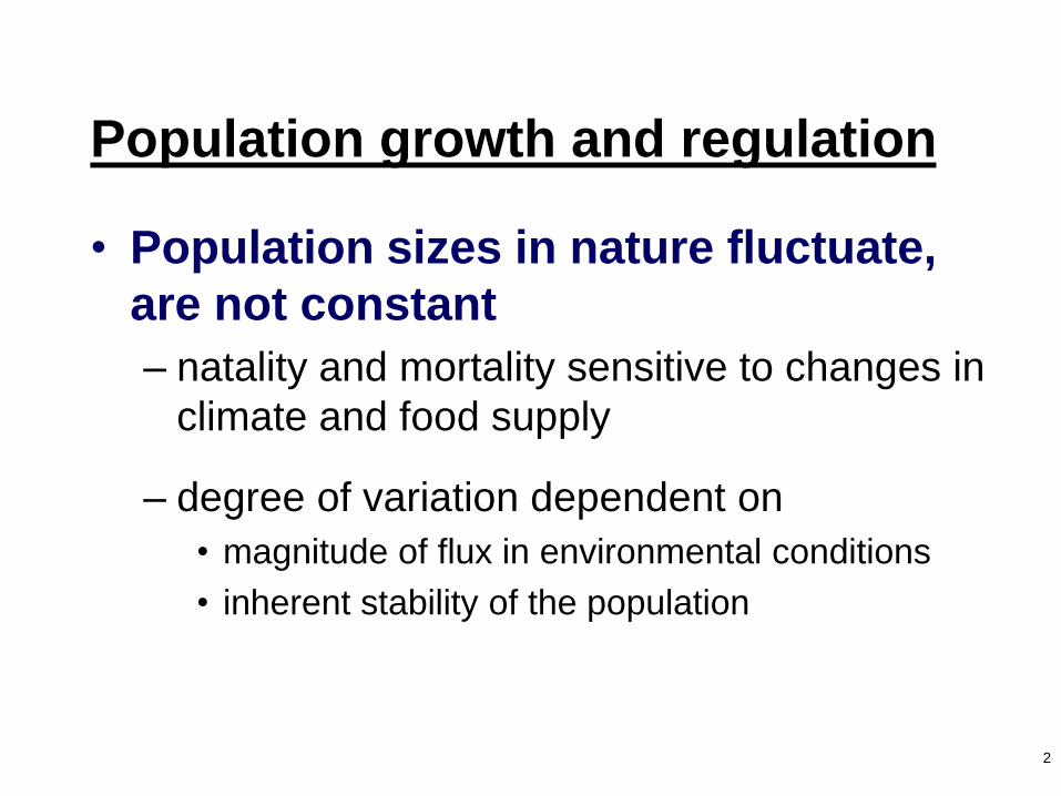
Population growth and regulation

• Population sizes in nature fluctuate,

are not constant

– natality and mortality sensitive to changes in

climate and food supply

– degree of variation dependent on

• magnitude of flux in environmental conditions

• inherent stability of the population

3

Number of sheep on the island of Tasmania since

their introduction in the early 1800s.

4

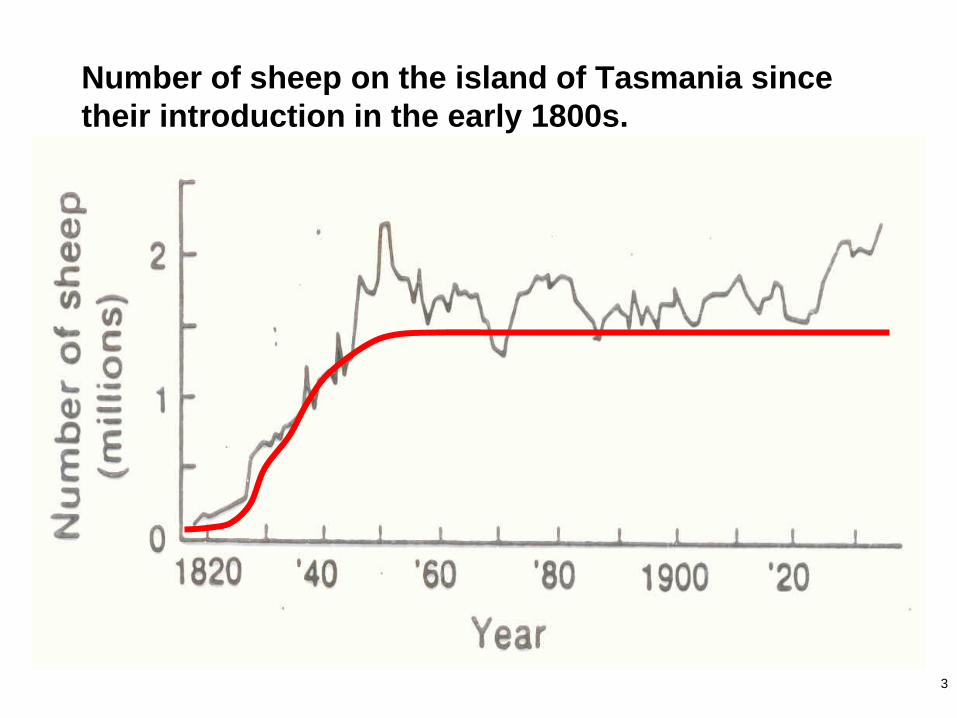
Population growth and regulation

• Population sizes in nature fluctuate,

are not constant

– short lived organisms are more sensitive to

environmental changes than long-lived

species

– limiting factor usually responsible for

population increases and decreases and is

often seasonal

5

Variation in the number of phytoplankton in samples

of water from Lake Erie during 1962.

6

Influences on population growth rates

• Stabilizing factors

– maintain population at equilibrium level

– density dependent

• Non-stabilizing factors

– no equilibrium level maintained

– density independent

7

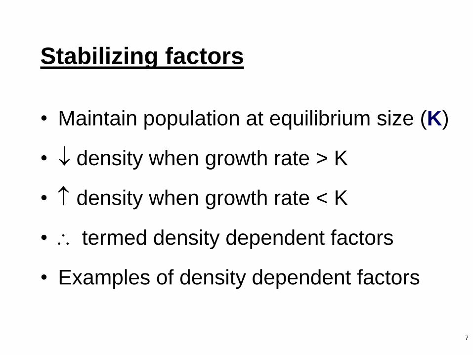
Stabilizing factors

• Maintain population at equilibrium size (K)

• density when growth rate > K

• density when growth rate < K

• termed density dependent factors

• Examples of density dependent factors

8

Hypothetical birth and death rates in a regulated

population.

9

Growth rate of a hypothetical population with respect

to increasing density.

10

Density approaching equilibrium in a hypothetical

population.

11

Fig. 9.1 (p. 144): Inherent growth potential of a

population; comparison of different reproductive rates

(starting N=10).

12

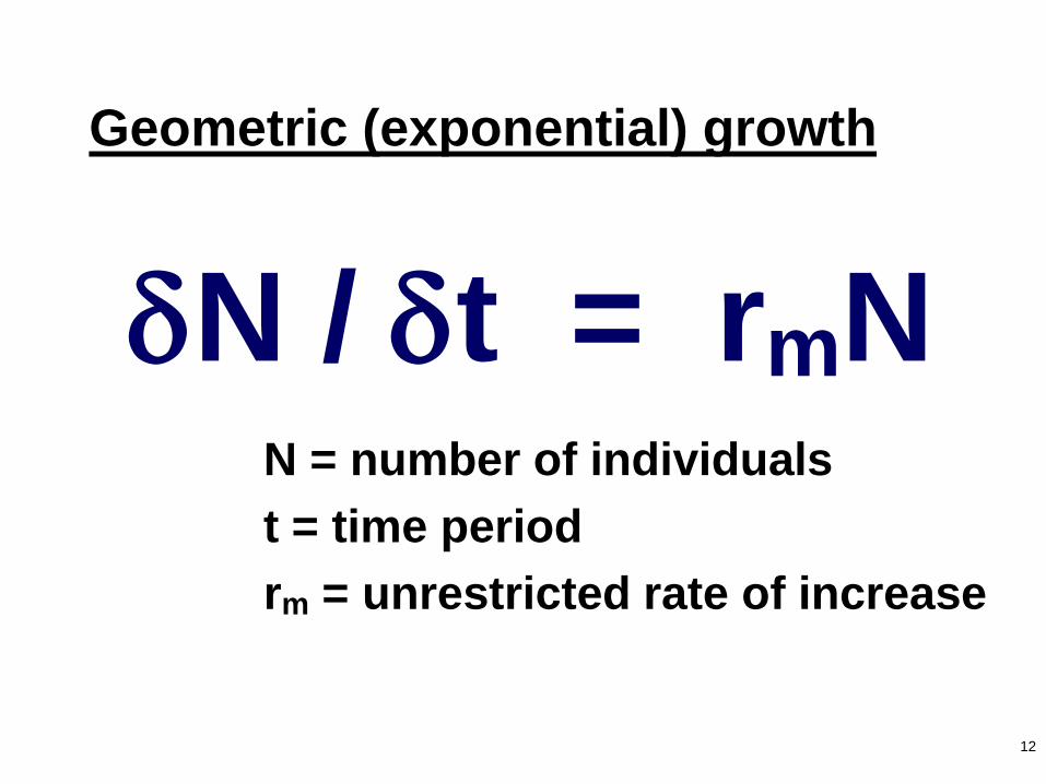
Geometric (exponential) growth

N / t = rmNN = number of individuals

t = time period

rm = unrestricted rate of increase

13

Geometric population growth

t N

0 2

1 4

2 8

3 16

4 32

5 64

6 128

7 256

8 512

9 1024

10 2048

11 4096

12 8192

13 16384

14 32768

15 65536

16 131072

17 262144

18 524288

19 1048576

20 2097152

0

500000

1000000

1500000

2000000

2500000

1 3 5 7 9 11 13 15 17 19 21

Nu

mb

er

in p

op

ula

tio

n

Time (Generation)

Plotted on arithmetic scale

14

Geometric population growth

t N

0 2

1 4

2 8

3 16

4 32

5 64

6 128

7 256

8 512

9 1024

10 2048

11 4096

12 8192

13 16384

14 32768

15 65536

16 131072

17 262144

18 524288

19 1048576

20 2097152

1

10

100

1000

10000

100000

1000000

10000000

1 3 5 7 9 11 13 15 17 19 21

Nu

mb

er

in p

op

ula

tio

n

Time (Generation)

Plotted on log scale

15

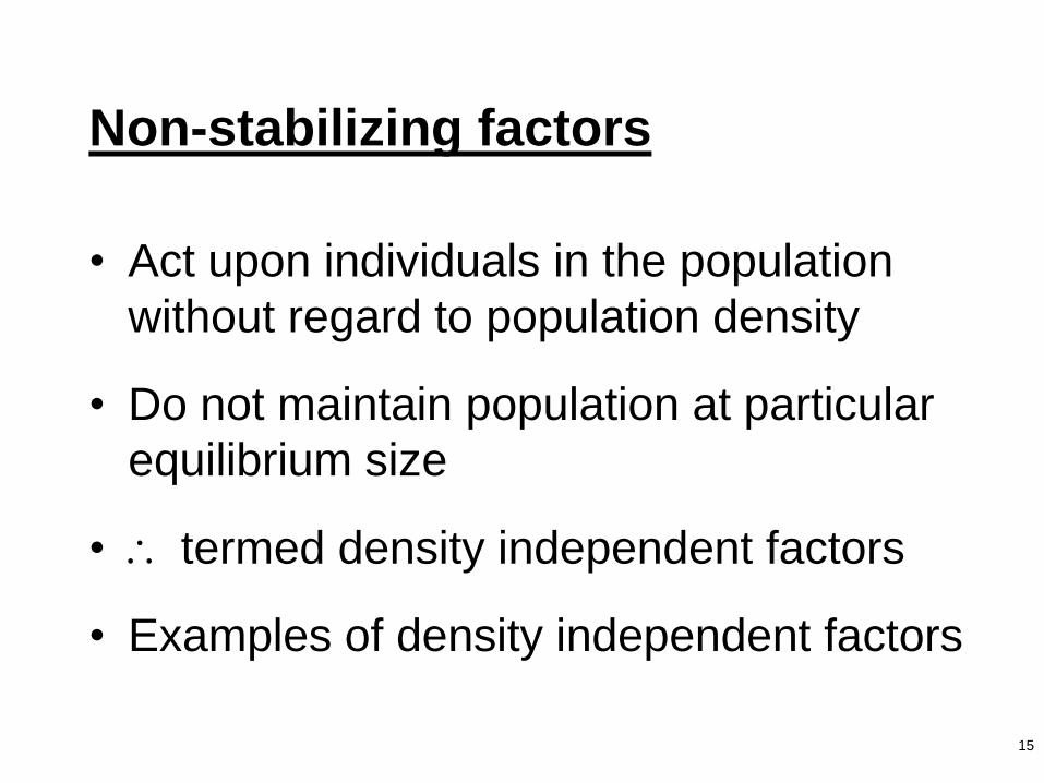
Non-stabilizing factors

• Act upon individuals in the population

without regard to population density

• Do not maintain population at particular

equilibrium size

• termed density independent factors

• Examples of density independent factors

16

Model for density dependent

population growth

• For any finite resource, there is an upper

limit to the number of individuals that can

utilize the resource

• Density dependent population growth is

based on

– geometric limitations

– availability of energy supply

– behavior (territoriality)

17

Logistic equation

• Pierre-François Verhulst (c 1835)

• Logistic (sigmoidal) growth curve

– population growth decreases as the

population size approaches the carrying

capacity (K) of the environment

• food, nutrients

• space

18

Fig. 9.4 (p. 146): Geometric (unlimited resources) versus

logistic (limited resources) growth of a population.

19

Logistic equation for growth of a

single population

N / t = rN [(K-N)/K]N = number of individuals

t = time period

r = unrestricted rate of increase

K = carrying capacity (upper asymptote)

20

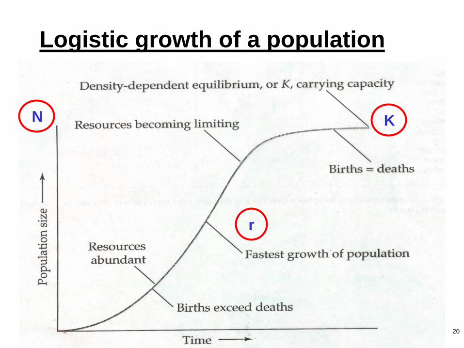
Logistic growth of a population

N

r

K

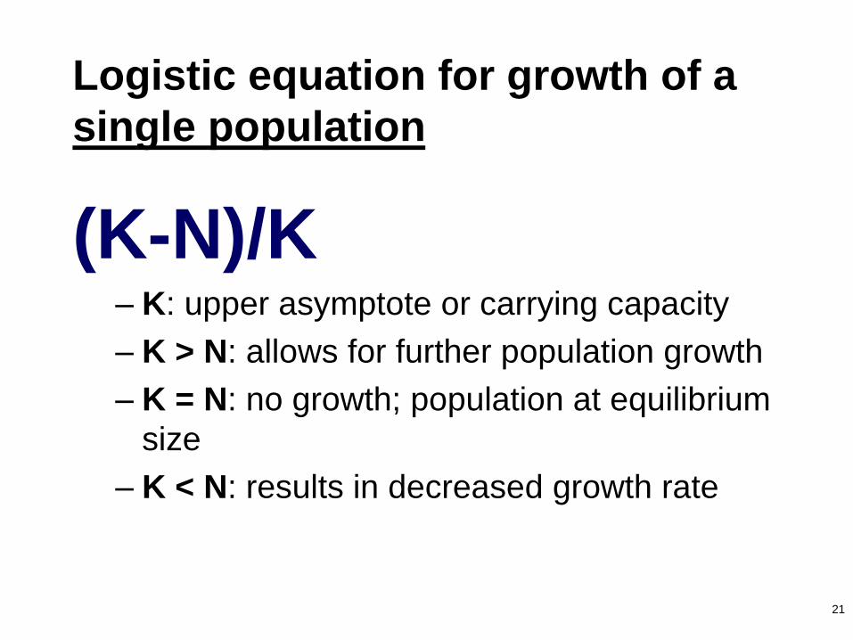
21

(K-N)/K– K: upper asymptote or carrying capacity

– K > N: allows for further population growth

– K = N: no growth; population at equilibrium

size

– K < N: results in decreased growth rate

Logistic equation for growth of a

single population

22

• Population increases determined by

– N: number of individuals present

– r: innate capacity for increase

– (K-N)/K: proportion of K not yet realized

Logistic equation for growth of a

single population

K = 100, N = 2: (K-N)/K = 98/100 = 0.98

δN/ δt = rN(0.98)

K = 100, N = 98: (K-N)/K = 2/100 = 0.02

δN/ δt = rN(0.02)

23

Logistic growth of a population

N

r

K

24

25

• (K-N)/K acts as negative feedback to

population growth

– when N is small

• (K-N)/K ~ 1

• r is maximal

• → exponential growth in population

Logistic equation for growth of a

single population

26

• (K-N)/K acts as negative feedback to

population growth

– as N increases

• (K-N)/K decreases

• ↓ actual rate of increase (ra)

Logistic equation for growth of a

single population

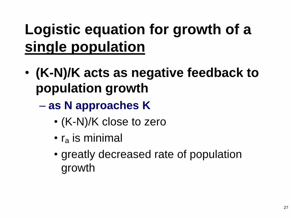
27

• (K-N)/K acts as negative feedback to

population growth

– as N approaches K

• (K-N)/K close to zero

• ra is minimal

• greatly decreased rate of population

growth

Logistic equation for growth of a

single population

28

Fig. 9.2 (p. 144): Net reproductive rate (r0) as a linear

function of population density (N) at time t.

29

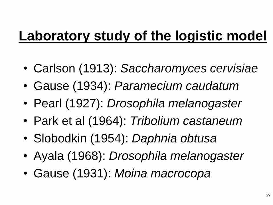
Laboratory study of the logistic model

• Carlson (1913): Saccharomyces cervisiae

• Gause (1934): Paramecium caudatum

• Pearl (1927): Drosophila melanogaster

• Park et al (1964): Tribolium castaneum

• Slobodkin (1954): Daphnia obtusa

• Ayala (1968): Drosophila melanogaster

• Gause (1931): Moina macrocopa

30

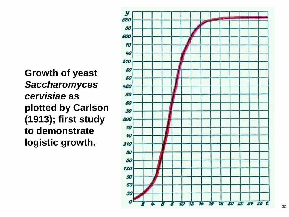
Growth of yeast

Saccharomyces

cervisiae as

plotted by Carlson

(1913); first study

to demonstrate

logistic growth.

31

Fig. 9.5 (p. 148): Population growth in the protozoans

Paramecium caudatum and P. aurelia (Gause 1934)

32

Fig. 9.6 (p. 149): Population growth of Drosophila

melanogaster under laboratory conditions (Pearl 1927).

Fig. 9.7 (p. 149): Population growth of two genetic

strains of the flour beetle Tribolium castaneum (Park et

al. 1964).

33

34

Relationship between K and food level in Daphnia

obtusa (Slobodkin 1954).

35

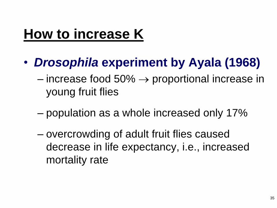
How to increase K

• Drosophila experiment by Ayala (1968)

– increase food 50% proportional increase in

young fruit flies

– population as a whole increased only 17%

– overcrowding of adult fruit flies caused

decrease in life expectancy, i.e., increased

mortality rate

36

How to increase K

• Drosophila experiment by Ayala (1968)

– increasing space increased overall population

density

– can increase K by increasing food and

space

37

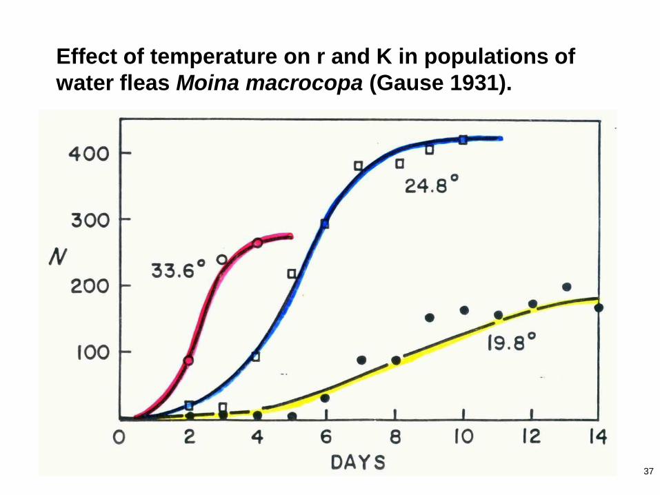
Effect of temperature on r and K in populations of

water fleas Moina macrocopa (Gause 1931).

38

Field study of the logistic model

• Ridgway et al. (2006): double-crested

cormorants on Lake Huron

• Saether et al. (2002): ibex in Switzerland

• Johns (2005): whooping cranes at Aransas,

Texas

• Scheffer (1951): reindeer on Pribilof Islands

• Walters et al. (1990): cladocerans in British

Columbia

39

Fig. 9.8 (p. 150): Growth in three colonies of double-

crested cormorants (Phalacrocorax auritus) on Lake

Huron, 1978-2003 (Ridgway et al. 2006).

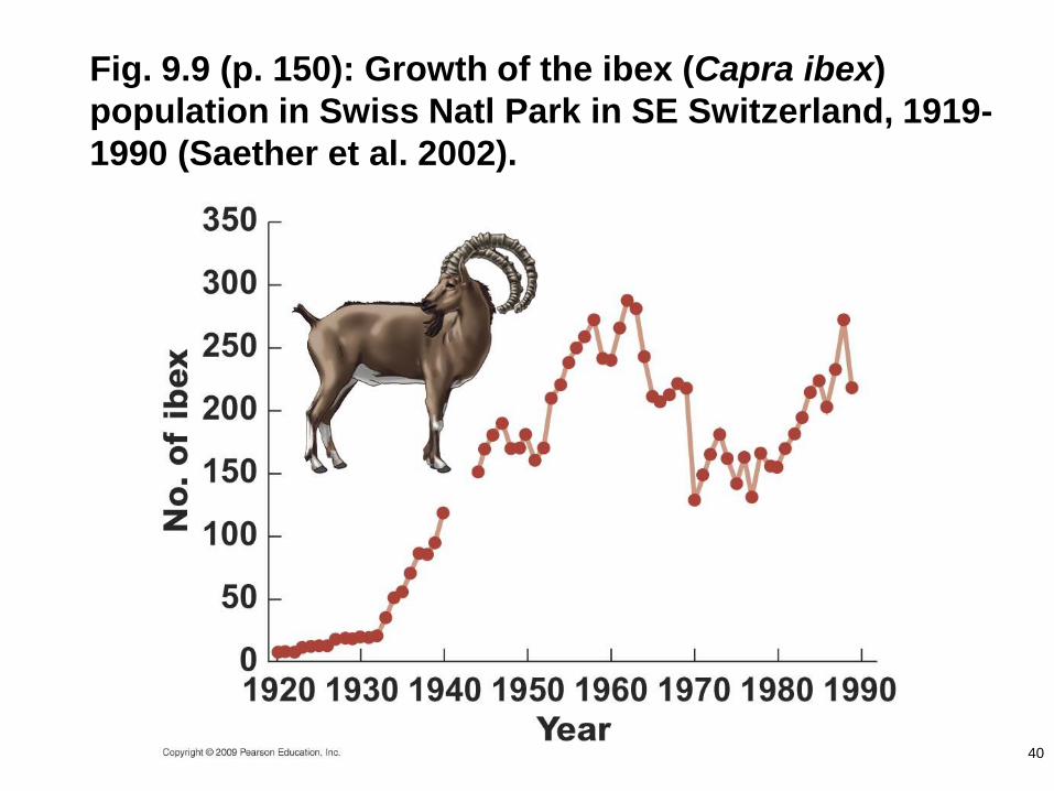
Fig. 9.9 (p. 150): Growth of the ibex (Capra ibex)

population in Swiss Natl Park in SE Switzerland, 1919-

1990 (Saether et al. 2002).

40

41

Fig. 9.10 (p. 151): Population growth in whooping cranes

(Aransas, TX) from near extinction in 1941 (Johns 2005).

42

Reindeer population growth on two Pribilof islands

following their introduction in 1911 (Scheffer 1951).

43

Fig. 9.11 (p. 151):

Population

fluctuations of

Daphnia rosea in

two British

Columbia lakes,

1980-1983

(Walters et al.

1990).

44

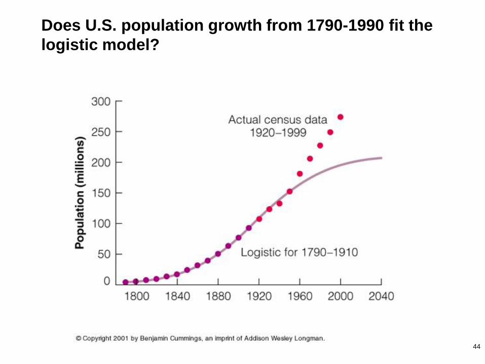
Does U.S. population growth from 1790-1990 fit the

logistic model?

45

Assumptions for the logistic model

• Population has a stable age distribution

– population characteristic

– stable age distribution: relative proportion of

individuals in each age class remains constant

over time

– rate of population change per age class = rate

of overall population change

– important assumption, usually not violated

46

Assumptions for the logistic model

• All individuals in the population are

equal

– all individuals use the same amount of

resources

– therefore, all individuals in the population are

assumed to be adults

– constantly violated

47

Assumptions for the logistic model

• r and K are constant and are real,

meaningful attributes of the population

– often violated

– few, if any, environments are constant over a

long period of time

– what is actually observed is some probability

distribution around K oscillations around the

asymptote driven by environmental changes

48

Fig. 9.15 (p.

154):

Population

growth in

Daphnia

magna in 50

ml of pond

water at (a)

18C and (b)

25C.

49

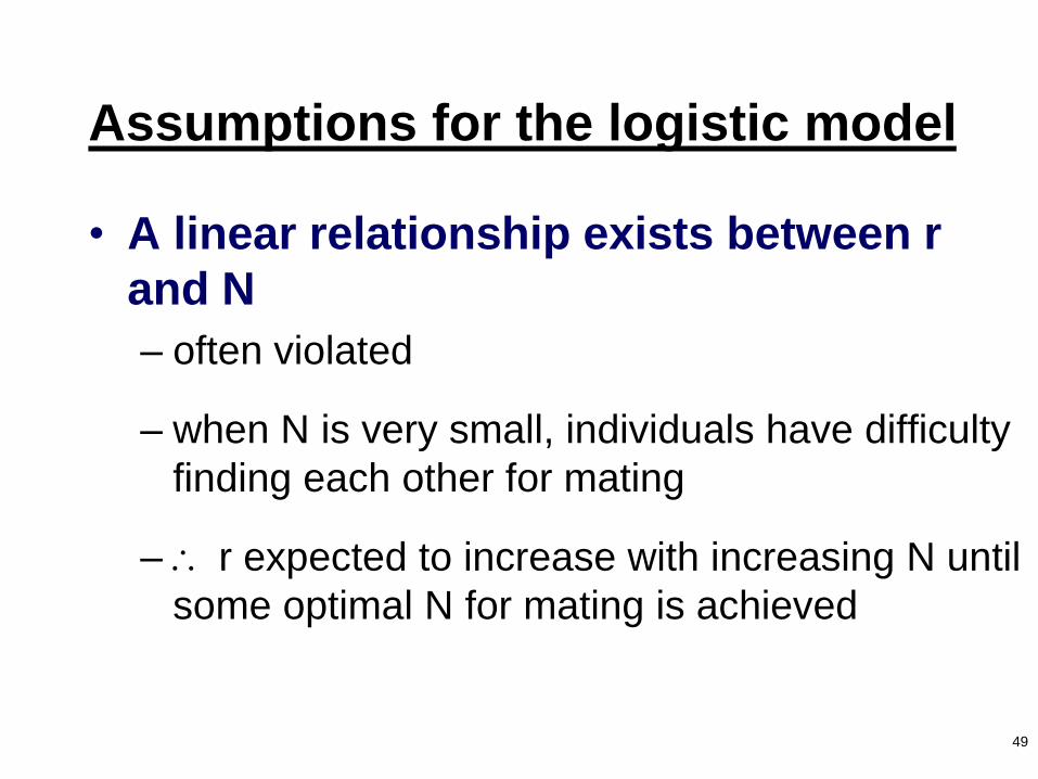
Assumptions for the logistic model

• A linear relationship exists between r

and N

– often violated

– when N is very small, individuals have difficulty

finding each other for mating

– r expected to increase with increasing N until

some optimal N for mating is achieved

50

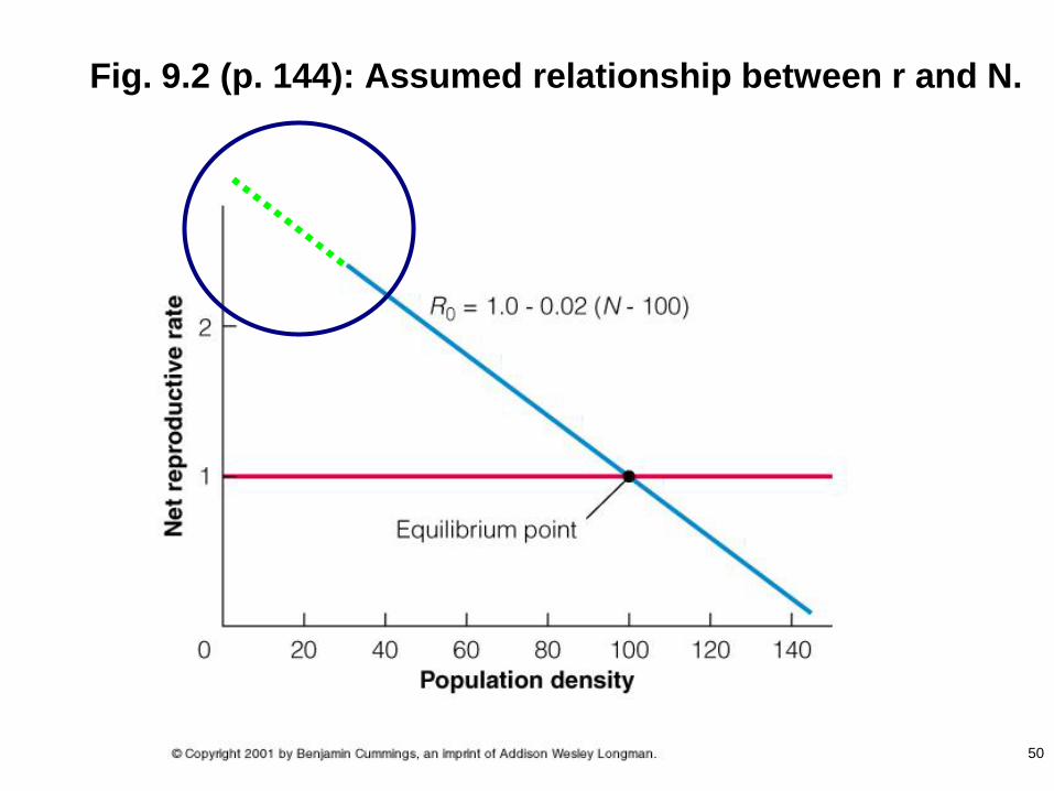
Fig. 9.2 (p. 144): Assumed relationship between r and N.

51

Fig. 9.2 (p. 144): More realistic view of the relationship

between r and N.

52

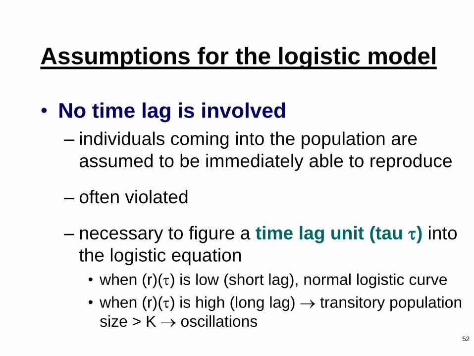
Assumptions for the logistic model

• No time lag is involved

– individuals coming into the population are

assumed to be immediately able to reproduce

– often violated

– necessary to figure a time lag unit (tau ) into

the logistic equation

• when (r)() is low (short lag), normal logistic curve

• when (r)() is high (long lag) transitory population

size > K oscillations

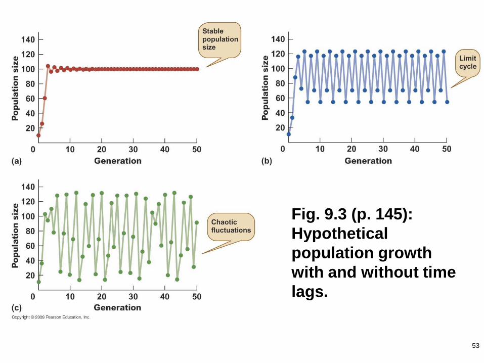
53

Fig. 9.3 (p. 145):

Hypothetical

population growth

with and without time

lags.

54

Conclusions regarding logistic

• Logistic equation fails to fit a lot of data from

the field

• Logistic model persists in ecology

because

– assumptions are well understood

– departures from the logistic model can be

attributed to violations of the assumptions

– logistic model is simple, easy to use

– no better model exists

55

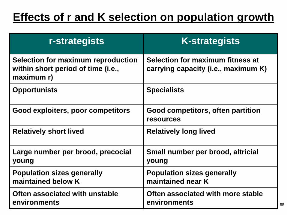
Effects of r and K selection on population growth

r-strategists K-strategists

Selection for maximum reproduction

within short period of time (i.e.,

maximum r)

Selection for maximum fitness at

carrying capacity (i.e., maximum K)

Opportunists Specialists

Good exploiters, poor competitors Good competitors, often partition

resources

Relatively short lived Relatively long lived

Large number per brood, precocial

young

Small number per brood, altricial

young

Population sizes generally

maintained below K

Population sizes generally

maintained near K

Often associated with unstable

environments

Often associated with more stable

environments