Chapter 9 Model Selection and Validation

Adapted from Timothy Hanson

Department of Statistics, University of South Carolina

Stat 704: Data Analysis I

1 / 22

Model building overview (pp.343-349)

Chapter 9: Model variable selection and validation

Book outlines four steps in data analysis

1 Data collection and preparation (acquiring and “cleaning”)

2 Reduction of explanatory variables (for exploratoryobservational studies). Mass screening for “decent” predictors.

3 Model refinement and selection.

4 Model validation.

We usually obtain data after step 1, though this step has receivedmuch more attention from statisticians in recent years.

2 / 22

9.1 Model building overview

Book has flowchart for model building process on p. 344.

Designed experiments are typically easy; experimentermanipulates treatment variables during experiment (andexpects them to be significant); experimenter may adjust forother variables.

With confirmatory observational studies, the goal is todetermine whether (or how) the response is related to one ormore pre-specified explanatory variables. No need to weedthem out.

Exploratory observational studies are done when we have littleprevious knowledge of exactly which predictors are related tothe response. Need to “weed out” good from uselesspredictors.

We may have a list of potentially useful predictors; variableselection can help us “screen out” useless ones and build agood, predictive model.

3 / 22

Controlled experiments

These include clinical trials, laboratory experiments onmonkeys and pigs, etc., community-based intervention trials,etc.

The experimenters control one or more variables that arerelated to the response. Often these variables are “treatment”and “control.” Can ascribe causality if populations are thesame except for the control variables.

Sometimes other variables (not experimentally assigned) thatmay also affect the response are collected too, e.g. gender,weight, blood chemistry levels, viral load, whether otherfamily members smoke, etc.

When building the model the treatment is always included.Other variables are included as needed to reduce variabilityand zoom in on the treatment factors. Some of thesevariables may be useful and some not, so part of the modelbuilding process is weeding out “noise” variables.

4 / 22

Confirmatory observational studies

Used to test a hypothesis built from other studies or a“hunch.”

Variables involved in the hypothesis (amount of fiber in diet)that affect the response (cholesterol) are measured along withother variables that can affect the outcome (age, exercise,gender, race, etc.) – nothing is controlled. Variables involvedin the hypothesis are called primary variables; the others arecalled risk factors; epidemiologists like to “adjust” for “riskfactors.”

Note that your book discusses Vitamin E and cancer on p.345. Such studies has received serious scrutiny recently.

Usually all variables are retained in the analysis; they werechosen ahead of time.

5 / 22

Observational studies

When people are involved, often not possible to conductcontrolled experiments.

Example: maternal smoking affects infant birthweight. Onewould have to randomly allocate the treatments “smoking”and “non-smoking” to pregnant moms – ethical problems.

Investigators consider anything that is easy to measure thatmight be related to the response. Many, many variables areconsidered, and models painstakingly built. One of myprofessors called this “data dredging.”

6 / 22

Observational studies

There’s a problem here – one is sure to find something if theylook hard enough. Often “signals” are there spuriously, andsometimes in the wrong direction.

The number of variables to consider can be large; there canbe high multicollinearity. Keeping too many predictors canmake prediction worse.

“The identification of “good”...variables to be included inthe...regression model and the determination of appropriatefunctional and interaction relations...constitute some of themost difficult problems in regression analysis.”

7 / 22

Section 9.2: GPA 2008 example

First steps often involve plots:

Plots to indicate correct functional form of predictors and/orresponse.Plots to indicate possible interaction.Exploration of correlation among predictors (maybe).Often a first-order model is a good starting point.

Once a reasonable set of potential predictors is identified,formal model selection begins.

If the number of predictors is large, say k ≥ 10, we can use(automated) stepwise procedures to reduce the number ofvariables (and models) under consideration.

8 / 22

9.3 Model selection (pp. 353-361)

Once we reduce the set of potential predictors to a reasonablenumber, we can examine all possible models and choose the “best”according to some criterion.

Say we have k predictors x1, . . . , xk and we want to find a goodsubset of predictors that predict the data well. There are severaluseful criteria to help choose a subset of predictors.

9 / 22

Adjusted-R2, R2a

“Regular” R2 measures how well the model predicts the data thatbuilt it. It is possible to have a model with R2 = 1 (predictsperfectly the data that built it), but has lousy out-of-sampleprediction. The adjusted R2, denoted R2

a , provide a “fix” to R2 toprovide a measure of how well the model will predict data not usedto build the model. For a candidate model with p − 1 predictors

R2a = 1− n − 1

n − p

SSEp

SSTO

(= 1− MSEp

s2y

).

Equivalent to choosing the model with the smallest MSEp.If irrelevant variables are added, R2

a may decrease unlike“regular” R2 (R2

a can be negative!).R2a penalizes model for being too complex.

Problem: R2a is greater for a “full” model whenever the

F-statistic for comparing full to reduced is greater than 1. Weusually want F-statistics to be a lot biggger than 1 beforeadding in new predictors =⇒ too liberal.

10 / 22

AIC

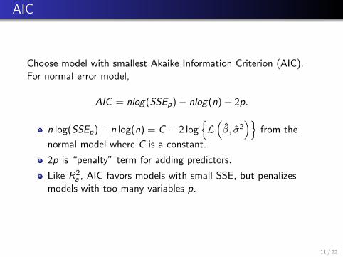
Choose model with smallest Akaike Information Criterion (AIC).For normal error model,

AIC = nlog(SSEp)− nlog(n) + 2p.

n log(SSEp)− n log(n) = C − 2 log{L(β, σ2

)}from the

normal model where C is a constant.

2p is “penalty” term for adding predictors.

Like R2a , AIC favors models with small SSE, but penalizes

models with too many variables p.

11 / 22

SBC (or BIC)

Models with smaller Schwarz Bayesian Criterion (SBC) areestimated to predict better. SBC is also known as BayesianInformation Criterion:

BIC = n log(SSEp)− n log(n) + p log(n).

BIC is similar to AIC, but for n ≥ 8, the BIC “penalty term” ismore severe.

Chooses model that “best predicts” the observed dataaccording to asymptotic criteria.

12 / 22

Mallow’s Cp

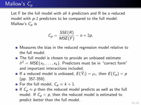
Let F be the full model with all k predictors and R be a reducedmodel with p-1 predictors to be compared to the full model.Mallow’s Cp is

Cp =SSE (R)

MSE (F )− n + 2p.

Measures the bias in the reduced regression model relative tothe full model.The full model is chosen to provide an unbiased estimateσ2 = MSE (x1, . . . , xk). Predictors must be in “correct form”and important interactions included.If a reduced model is unbiased, E (Yi ) = µi , then E (Cp) = p(pp. 357-359).For the full model, Cp ≡ k + 1.If Cp ≈ p then the reduced model predicts as well as the fullmodel. If Cp < p, then the reduced model is estimated topredict better than the full model.

13 / 22

Which criteria to use?

R2a , AIC, BIC, and Cp may give different “best” models, or they

may agree. The ultimate goal is to find model(s) that balance(s):

A good fit to the data.

Low bias.

Parsimony.

All else being equal, the simpler model is often easier to interpretand work with. Christensen (1996) recommends Cp and notes thesimilarity between Cp and AIC.

14 / 22

Two methods for “automatically” picking variables

Two automated methods for variable selection are bestsubsets and stepwise procedures.

Best subsets simply finds the models that are best accordingto some statistic, e.g., smallest Cp of a given size. Only proc

reg does this automatically, but does not enforce hierarchicalmodel building; grouping of coded categorical variables isignored as well.

Stepwise procedures add and/or subtract variables one at atime according to prespecified inclusions/exclusion criteria.Useful when you have a very large number of variables (e.g.,k > 30). Both proc reg and proc glmselect incorporatestepwise methods.

15 / 22

Best subsets for Fall 2008 GPA data

Refer to the text example for a best subsets regression withcontinuous variables and interactions. The Fall 2008 data setincludes a response (GPA), two continuous predictors (Verbal SATand Math SAT) and numerous categorical predictors. We recodedthe categorical predictors with a modest number of categories(Class, Race, Gender, Enrollment Status, Registration Status) andincluded each main effect as a set.

data fall08; set fall08;

proc reg data=fall08;

model cltotgpa=satv satm class2 class3 class4 housing raceaa raceo raceu

genderf enrollft regn rego/selection=cp best=10;

run;

16 / 22

9.4 automated variable search (pp. 361–368)

Forward stepwise regression (pp. 364–365)We start with k potential predictors x1, . . . , xk . We add and deletepredictors one at a time until all predictors are significant at somepreset level. Let αe be the significance level for adding variables,and αr be significance level for removing them.

Note: We should choose αe < αr ; in book example, αe = 0.1 &αr = 0.15.

17 / 22

Forward stepwise regression

1 Regress Y on x1 only, Y on x2 only, up to Y on xk only. Ineach case, look at the p-value for testing the slope is zero.Pick the x variable with the smallest p-value to include in thethe model.

2 Fit all possible 2-predictor models (in general j-predictormodels) that include the initially chosen x , along with eachremaining x variable in turn. Pick new x variable withsmallest p-value for testing slope equal to zero in model thatalready has first one chosen, as long as p-value < αe . Maybenothing is added.

3 Remove the x variable with the largest p-value as long asp-value > αr . Maybe nothing is removed.

4 Repeat steps (2)-(3) until no x variables can be added orremoved.

18 / 22

proc glmselect

Forward selection and backward elimination are similarprocedures; see p. 368. I suggest stepwise of the three.

proc glmselect implements automated variable selectionmethods for regression models.

Does stepwise, backwards, and forwards procedures as well asleast angle regression (LAR) and lasso. Flom and Casell(2007) recommend either of these last two over all traditionalstepwise approaches & note they both perform about thesame.

The syntax is the same as proc glm, and you can includeclass variables, interactions, etc.

19 / 22

proc glmselect

The hier=single option buildes hierarchical models. To dostepwise as in your textbook, include select=sl. You canalso use any of AIC, BIC, Cp, or R2

a rather than p-valuecutoffs for model selection.

proc glmselect will stop when you cannot add or removeany predictors, but the “best” model may have been found inan earlier iteration. Using choose=cp, for example, gives themodel with the lowest Cp as the final model, regardless wherethe procedure stops.

include=p includes the first p variables listed in the modelstatement in every model. Why might this be necessary?

20 / 22

proc glmselect

Fall 2008 enrollment data: Stepwise selection, choosinghierarchical model with smallest Cp during stepwise procedure.

proc glmselect;

class class race regstatus gender enroll housing

model cltotgpa=satv satm class housing race gender enroll regstat

satv*race satv*gender satv*enroll satm*race satm*gender satm*enroll/select=sl

sle=0.1 sls=0.15 hier=single;

run;

The most interesting part of this analysis was actually the EDAthat identified a previously-overlooked problem with theRegistration Status variable.

21 / 22

Stepwise procedures vs. best subsets

Forward selection, backward elimination, and stepwiseprocedures are designed for very large numbers of variables.

Best subsets works well when the number of potentialvariables is smaller. You can identify best subsets in proc

reg, but SAS will not weed out non-hierarchical models.

Choose proc glmselect for “large p” problems and chooseproc reg for smaller numbers of predictors, e.g., k < 30.

22 / 22