Chapter 9The Blahut-Arimoto

Algorithms

© Raymond W. Yeung 2012

Department of Information EngineeringThe Chinese University of Hong Kong

Single-Letter Characterization

• For a DMC p(y|x), the capacity

C = max

r(x)I(X;Y ),

where r(x) is the input distribution, gives the maximum asymptotically

achievable rate for reliable communication as the blocklength n!1.

• This characterization of C, in the form of an optimization problem, is

called a single-letter characterization because it involves only p(y|x) but

not n.

• Similarly, the rate-distortion function

R(D) = min

Q(x̂|x):Ed(X,X̂)D

I(X;

ˆ

X)

for an i.i.d. information source {Xk

} is a single-letter characterization.

Numerical Methods

• When the alphabets are finite, C and R(D) are given as solutions of finite-dimensional optimization problems.

• However, these quantities cannot be expressed in closed-forms except forvery special cases.

• Even computing these quantities is not straightforward because the asso-ciated optimization problems are nonlinear.

• So we have to resort to numerical methods.

• The BA algorithms are iterative algorithms devised for this purpose.

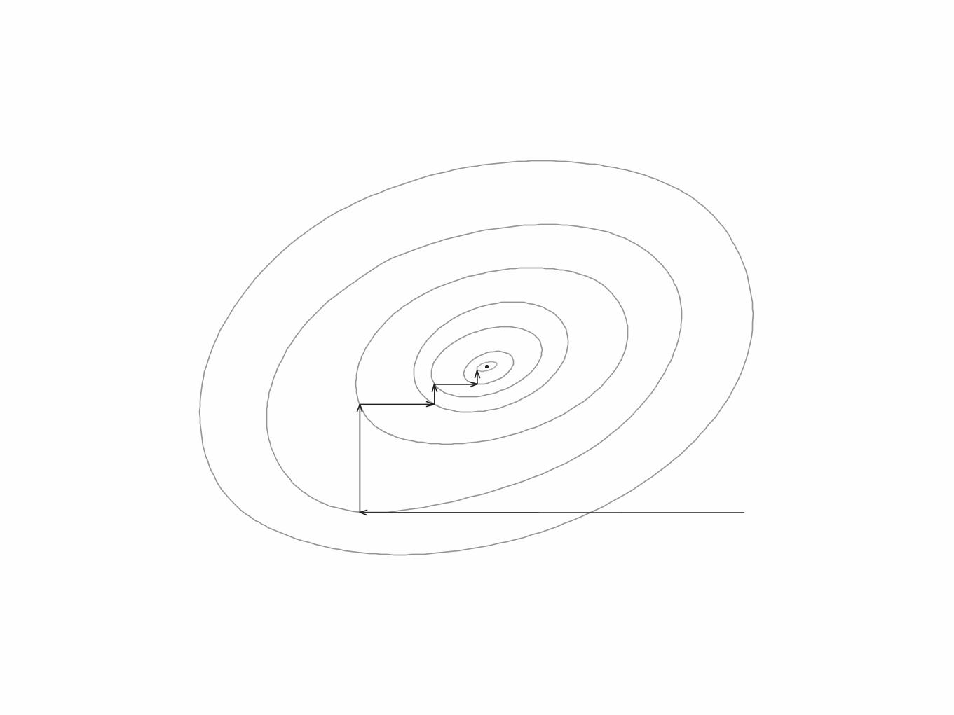
9.1 Alternating OptimizationConsider the double supremum

sup

u12A1

sup

u22A2

f(u1,u2).

• Ai is a convex subset of <nifor i = 1, 2.

• f : A1 ⇥A2 ! < is bounded from above, such that

– f is continuous and has continuous partial derivatives on A1 ⇥A2;

– For all u2 2 A2, there exists a unique c1(u2) 2 A1 such that

f(c1(u2),u2) = max

u012A1

f(u01,u2),

and for all u1 2 A1, there exists a unique c2(u1) 2 A2 such that

f(u1, c2(u1)) = max

u022A2

f(u1,u02).

• Let u = (u1,u2) and A = A1 ⇥ A2. Then the double supremum can be

written as

sup

u2Af(u).

• In other words, the supremum of f is taken over a subset of <n1+n2which

is equal to the Cartesian product of two convex subsets of <n1and <n2

,

respectively.

• Let f⇤ denote this supremum.

An Alternating Optimization Algorithm for Computing f*

• Let u(k)= (u(k)

1 ,u(k)2 ) for k � 0, defined as follows.

• Let u(0)1 be an arbitrarily chosen vector in A1, and let u(0)

2 = c2(u(0)1 ).

• For k � 1, u(k)is defined by

u(k)1 = c1(u

(k�1)2 )

and

u(k)2 = c2(u

(k)1 ).

• Let

f (k)= f(u(k)

).

• Then

f (k) � f (k�1).

• Since the sequence f (k)is non-decreasing, it must converge because f is

bounded from above.

• We will show that f (k) ! f⇤ if f is concave.

• Replacing f by �f , the double supremum becomes the double infimum

inf

u12A1inf

u22A2f(u1,u2).

• The same alternating optimization algorithm can be applied to compute

this infimum.

9.2 The Algorithms

• The alternating optimization algorithm is specialized for computing C and

R(D).

9.2.1 Channel CapacityLemma 9.1 Let r(x)p(y|x) be a given joint distribution on X ⇥ Y such that

r > 0, and let q be a transition matrix from Y to X . Then

max

q

X

x

X

y

r(x)p(y|x) log

q(x|y)

r(x)

=

X

x

X

y

r(x)p(y|x) log

q

⇤(x|y)

r(x)

,

where the maximization is taken over all q such that

q(x|y) = 0 if and only if p(y|x) = 0, (1)

and

q

⇤(x|y) =

r(x)p(y|x)Px

0 r(x

0)p(y|x0

)

, (2)

i.e., the maximizing q is the one which corresponds to the input distribution rand the transition matrix p(y|x).

Proof

1. In (2), let

w(y) =

X

x

0

r(x

0)p(y|x0

).

2. Assume w.l.o.g. that for all y 2 Y, p(y|x) > 0 for some x 2 X .

3. Since r > 0, w(y) > 0 for all y, and hence q

⇤(x|y) is well-defined.

4. Rearranging (2), we have

r(x)p(y|x) = w(y)q

⇤(x|y).

5. Consider

X

x

X

y

r(x)p(y|x) log

q

⇤(x|y)

r(x)

�X

x

X

y

r(x)p(y|x) log

q(x|y)

r(x)

=

X

x

X

y

r(x)p(y|x) log

q

⇤(x|y)

q(x|y)

=

X

y

X

x

w(y)q

⇤(x|y) log

q

⇤(x|y)

q(x|y)

=

X

y

w(y)

X

x

q

⇤(x|y) log

q

⇤(x|y)

q(x|y)

=

X

y

w(y)D(q

⇤(x|y)kq(x|y))

� 0.

6. The proof is completed by noting in (2) that q⇤ satisfies (1) because r > 0.

Theorem 9.2 For a discrete memoryless channel p(y|x),

C = sup

r>0max

q

X

x

X

y

r(x)p(y|x) log

q(x|y)

r(x)

,

where the maximization is taken over all q that satisfies (1) in Lemma 9.1.

Proof

• Write I(X;Y ) as I(r,p) where r is the input distribution and p denotes

the transition matrix of the generic channel p(y|x). Then

C = max

r�0I(r,p).

• By Lemma 9.1, we need to prove that

C = max

r�0I(r,p) = sup

r>0I(r,p).

• Let r

⇤achieves C.

• If r⇤ > 0, then

C = max

r�0I(r,p) = max

r>0I(r,p) = sup

r>0I(r,p).

• Next, consider r⇤ � 0. Since I(r,p) is continuous in r, for any ✏ > 0, there

exists � > 0 such that if

kr� r⇤k < �,

then

C � I(r,p) < ✏,

• In particular, there exists

˜r > 0 such that k˜r� r⇤k < �.

• Then

C = max

r�0I(r,p) � sup

r>0I(r,p) � I(

˜r,p) > C � ✏.

• Let ✏ ! 0 to conclude that

C = sup

r>0I(r,p).

Recall the double supremum in Section 9.1:

sup

u12A1

sup

u22A2

f(u1,u2).

• Ai is a convex subset of <nifor i = 1, 2.

• f : A1 ⇥A2 ! < is bounded from above, such that

– f is continuous and has continuous partial derivatives on A1 ⇥A2;

– For all u2 2 A2, there exists a unique c1(u2) 2 A1 such that

f(c1(u2),u2) = max

u012A1

f(u01,u2),

and for all u1 2 A1, there exists a unique c2(u1) 2 A2 such that

f(u1, c2(u1)) = max

u022A2

f(u1,u02).

Cast the computation of C into this optimization problem:

• Let

f(r,q) =X

x

X

y

r(x)p(y|x) log q(x|y)r(x)

,

where u1 r and u2 q.

• Let

A1 = {(r(x), x 2 X ) : r(x) > 0 and

Px

r(x) = 1} ⇢ <|X |

and

A2 = {(q(x|y), (x, y) 2 X ⇥ Y) : q(x|y) > 0 i↵ p(y|x) > 0,

and

Px

q(x|y) = 1 for all y 2 Y}⇢ <|X ||Y|

.

Remarks

• Both A1 and A2 are convex.

• f is bounded from above.

• In f(r,q), the double summation by convention is over all x such that

r(x) > 0 and all y such that p(y|x) > 0.

• Since q(x|y) > 0 whenever p(y|x) > 0, all the probabilities involved in the

double summation are positive.

• Therefore, f is continuous and has continuous partial derivatives on A =

A1 ⇥A2.

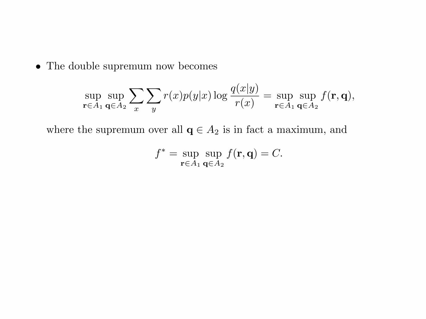
• The double supremum now becomes

sup

r2A1

sup

q2A2

X

x

X

y

r(x)p(y|x) log q(x|y)r(x)

= sup

r2A1

sup

q2A2

f(r,q),

where the supremum over all q 2 A2 is in fact a maximum, and

f

⇤= sup

r2A1

sup

q2A2

f(r,q) = C.

Algorithm Details• By Lemma 9.1, for any given r 2 A1, there exists a unique q 2 A2 that

maximizes f .

• By Lagrange multiplies, it can be shown that for a given q 2 A2, the input

distribution r that maximizes f is given by

r(x) =

Qy

q(x|y)

p(y|x)

Px

0Q

y

q(x

0|y)

p(y|x0),

where the product is over all y such that p(y|x) > 0, and q(x|y) > 0 for

all such y. This implies r > 0 and hence r 2 A1.

• Let r(0)an arbitrarily chosen strictly positive input distribution in A1.

Then q(0) 2 A2 can be determined accordingly. This forms (r(0),q(0)

).

• Compute (r(k),q(k)

), k � 1 iteratively.

• It will be shown in Section 9.3 that f

(k)= f(r(k)

,q(k))! f

⇤= C.

9.2.2 The Rate-Distortion Function

• Assume R(0) > 0, so that R(D) is strictly decreasing for 0 D Dmax

.

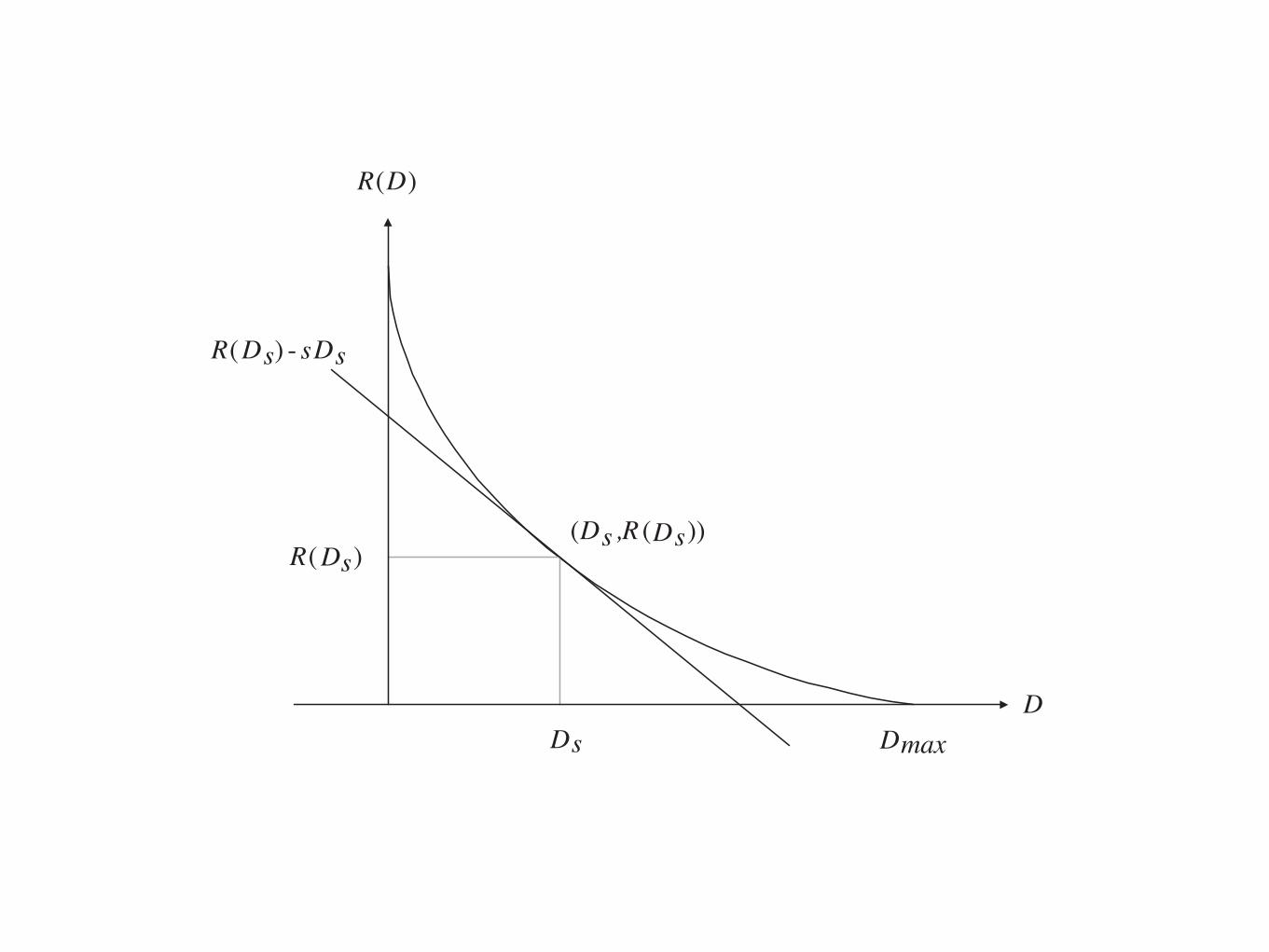
• Since R(D) is convex, for any s 0, there exists a point on the R(D)

curve for 0 D Dmax

such that the slope of a tangent to the R(D)

curve at that point is equal to s.

• Denote such a point on the R(D) curve by (Ds

, R(Ds

)), which is not

necessarily unique.

• Then this tangent intersects with the ordinate at R(Ds

)� sDs

.

D

R ( D )

D s

R ( ) D s

R ( ) - s D s

D max

D s

( ,R ( )) D s D s

• Write I(X;

ˆX) and Ed(X, ˆX) as I(p,Q) and D(p,Q), respectively, where

p is the distribution for X and Q is the transition matrix from X to

ˆXdefining

ˆX.

• For any Q, (D(p,Q), I(p,Q)) is a point in the rate-distortion region, and

the line with slope s passing through (D(p,Q), I(p,Q)) intersects the

ordinate at I(p,Q)� sD(p,Q).

• Then

R(Ds)� sDs = min

Q[I(p,Q)� sD(p,Q)]. (1)

• By varying over all s 0, we can then trace out the whole R(D) curve.

Lemma 9.3 Let p(x)Q(x̂|x) be a given joint distribution on X ⇥ ˆX such that

Q > 0, and let t be any distribution on

ˆX such that t > 0. Then

min

t>0

X

x

X

x̂

p(x)Q(x̂|x) log

Q(x̂|x)

t(x̂)

=

X

x

X

x̂

p(x)Q(x̂|x) log

Q(x̂|x)

t

⇤(x̂)

, (2)

where

t

⇤(x̂) =

X

x

p(x)Q(x̂|x),

i.e., the minimizing t is the one which corresponds to the input distribution pand the transition matrix Q.

Remarks:

• t⇤ > 0 because Q > 0.

• The right-hand side of (2) is equal to I(p,Q).

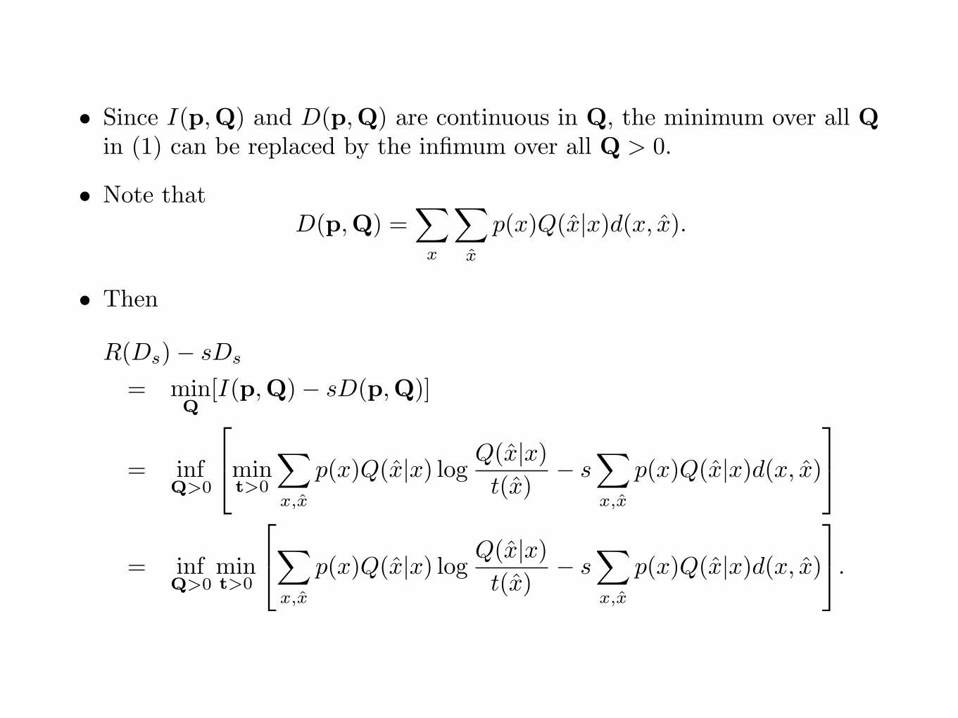
• Since I(p,Q) and D(p,Q) are continuous in Q, the minimum over all Qin (1) can be replaced by the infimum over all Q > 0.

• Note that

D(p,Q) =

X

x

X

x̂

p(x)Q(x̂|x)d(x, x̂).

• Then

R(D

s

)� sD

s

= min

Q[I(p,Q)� sD(p,Q)]

= inf

Q>0

2

4min

t>0

X

x,x̂

p(x)Q(x̂|x) log

Q(x̂|x)

t(x̂)

� s

X

x,x̂

p(x)Q(x̂|x)d(x, x̂)

3

5

= inf

Q>0min

t>0

2

4X

x,x̂

p(x)Q(x̂|x) log

Q(x̂|x)

t(x̂)

� s

X

x,x̂

p(x)Q(x̂|x)d(x, x̂)

3

5.

Recall the double infimum in Section 9.1:

inf

u12A1

inf

u22A2

f(u1,u2).

• Ai is a convex subset of <nifor i = 1, 2.

• f : A1 ⇥A2 ! < is bounded from below, such that

– f is continuous and has continuous partial derivatives on A1 ⇥A2;

– For all u2 2 A2, there exists a unique c1(u2) 2 A1 such that

f(c1(u2),u2) = min

u012A1

f(u01,u2),

and for all u1 2 A1, there exists a unique c2(u1) 2 A2 such that

f(u1, c2(u1)) = min

u022A2

f(u1,u02).

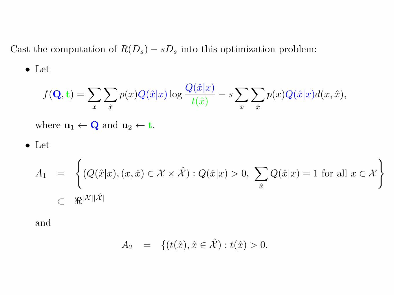
Cast the computation of R(D

s

)� sD

s

into this optimization problem:

• Let

f(Q, t) =X

x

X

x̂

p(x)Q(x̂|x) log Q(x̂|x)t(x̂)

� s

X

x

X

x̂

p(x)Q(x̂|x)d(x, x̂),

where u1 Q and u2 t.

• Let

A1 =

((Q(x̂|x), (x, x̂) 2 X ⇥ ˆX ) : Q(x̂|x) > 0,

X

x̂

Q(x̂|x) = 1 for all x 2 X)

⇢ <|X ||X̂ |

and

A2 = {(t(x̂), x̂ 2 ˆX ) : t(x̂) > 0.

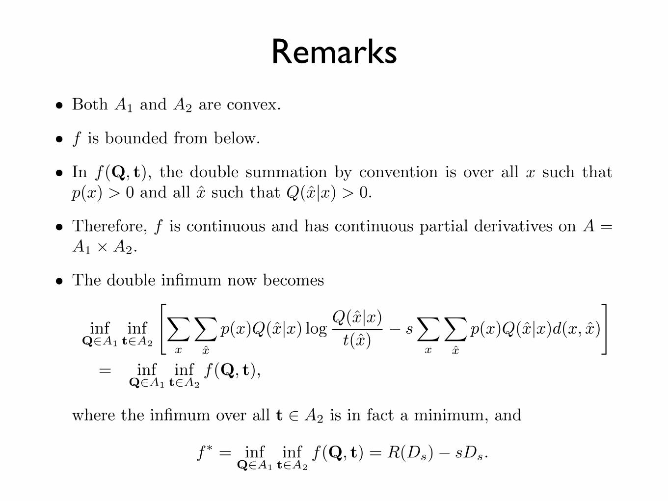
Remarks• Both A1 and A2 are convex.

• f is bounded from below.

• In f(Q, t), the double summation by convention is over all x such that

p(x) > 0 and all x̂ such that Q(x̂|x) > 0.

• Therefore, f is continuous and has continuous partial derivatives on A =

A1 ⇥A2.

• The double infimum now becomes

inf

Q2A1

inf

t2A2

"X

x

X

x̂

p(x)Q(x̂|x) log Q(x̂|x)t(x̂)

� s

X

x

X

x̂

p(x)Q(x̂|x)d(x, x̂)#

= inf

Q2A1

inf

t2A2

f(Q, t),

where the infimum over all t 2 A2 is in fact a minimum, and

f

⇤= inf

Q2A1

inf

t2A2

f(Q, t) = R(D

s

)� sD

s

.

Algorithm Details• By Lemma 9.3, for any given Q 2 A1, there exists a unique t 2 A2 that

minimizes f .

• By Lagrange multipliers, it can be shown that for a given t 2 A2, the

transition matrix Q that minimizers f is given by

Q(x̂|x) =

t(x̂)e

sd(x,x̂)

Px̂

0 t(x̂

0)e

sd(x,x̂

0)> 0,

and so Q 2 A1.

• Let Q(0)an arbitrarily chosen strictly positive transition matrix in A1.

Then t(0) 2 A2 can be determined accordingly. This forms (Q(0), t(0)

).

• Compute (Q(k), t(k)

), k � 1 iteratively.

• It will be shown in Section 9.3 that f

(k)= f(Q(k)

, t(k))! f

⇤= R(D

s

)�sD

s

.

9.3 Convergence

• Consider the double supremum optimization problem in Section 9.1.

• We first prove in general that if f is concave, then f (k) ! f⇤.

• We then apply this su�cient condition to prove the convergence of the

BA algorithm for computing C.

• The convergence of the BA algorithm for computing R(Ds)� sDs can be

proved likewise.

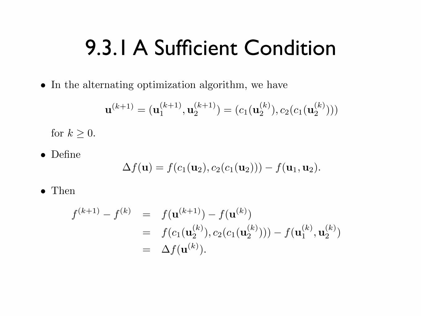
9.3.1 A Sufficient Condition

• In the alternating optimization algorithm, we have

u(k+1)= (u(k+1)

1 ,u(k+1)2 ) = (c1(u

(k)2 ), c2(c1(u

(k)2 )))

for k � 0.

• Define

�f(u) = f(c1(u2), c2(c1(u2)))� f(u1,u2).

• Then

f (k+1) � f (k)= f(u(k+1)

)� f(u(k))

= f(c1(u(k)2 ), c2(c1(u

(k)2 )))� f(u(k)

1 ,u(k)2 )

= �f(u(k)).

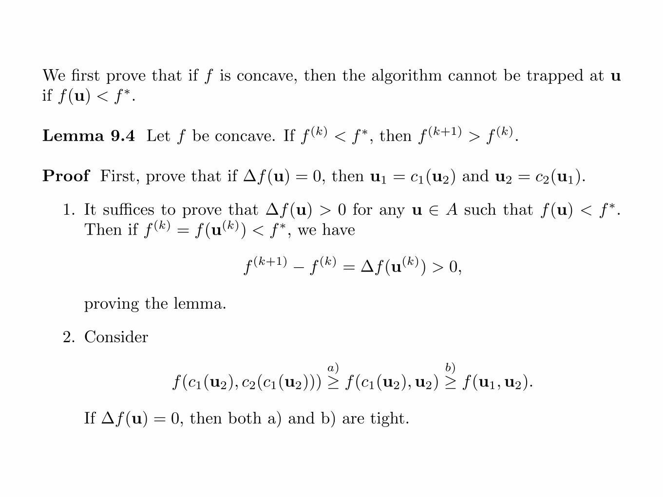
We first prove that if f is concave, then the algorithm cannot be trapped at u

if f(u) < f⇤.

Lemma 9.4 Let f be concave. If f (k) < f⇤, then f (k+1) > f (k)

.

Proof First, prove that if �f(u) = 0, then u1 = c1(u2) and u2 = c2(u1).

1. It su�ces to prove that �f(u) > 0 for any u 2 A such that f(u) < f⇤.

Then if f (k)= f(u(k)

) < f⇤, we have

f (k+1) � f (k)= �f(u(k)

) > 0,

proving the lemma.

2. Consider

f(c1(u2), c2(c1(u2)))a)� f(c1(u2),u2)

b)� f(u1,u2).

If �f(u) = 0, then both a) and b) are tight.

3. Due to the uniqueness of c2(·) and c1(·),

b) is tight ) u1 = c1(u2)

a) is tight ) u2 = c2(c1(u2)) = c2(u1).

4. This also implies that if f (k+1)�f (k)= �f(u(k)

) = 0, then u(k+1)= u(k)

.

Second, consider any u 2 A such that f(u) < f⇤. Prove by contradiction that

�f(u) > 0.

1. Assume that �f(u) = 0. Then u1 = c1(u2) and u2 = c2(u1), i.e., u1

maximizes f for a fixed u2, and u2 maximizes f for a fixed u1.

2. Since f(u) < f⇤, there exists v 2 A such that f(u) < f(v).

3. Let

˜z unit vector in the direction of v � u

z1 unit vector in the direction of (v1 � u1, 0)

z2 unit vector in the direction of (0,v2 � u2).

z

z 1

z 2

( u u ) 1 2 , ( v u ) 1 2 ,

( u v ) 1 2 , ( v v ) 1 2 ,

4. Then z̃ = ↵1z1 + ↵2z2, where

↵i =kvi � uikkv � uk , i = 1, 2.

5. Since f is continuous and has continuous partial derivatives, the direc-tional derivative of f at u in the direction of z1 is given by 5f · z1.

6. f attains its maximum value at u = (u1,u2) when u2 is fixed.

7. In particular, f attains its maximum value at u along the line passingthrough (u1,u2) and (v1,u2).

8. It follows from the concavity of f along the line passing through (u1,u2)and (v1,u2) that 5f · z1 = 0. Similarly, 5f · z2 = 0.

9. Then 5f · z̃ = ↵1(5f · z1) + ↵2(5f · z2) = 0.

10. Since f is concave along the line passing through u and v, this impliesf(u) � f(v), a contradiction.

11. Hence, �f(u) > 0.

Although �f(u) > 0 as long as f(u) < f⇤, f (k) does not necessarily convergeto f⇤ because the increment in f (k) in each step may be arbitrarily small.

Theorem 9.5 If f is concave, then f (k) ! f⇤.

Proof

1. f (k) necessarily converges, say to f 0, because f (k) is nondecreasing andbounded from above.

2. Hence, for any ✏ > 0 and all su�ciently large k,

f 0 � ✏ f (k) f 0. (1)

3. Let� = min

u2A0�f(u),

where A0 = {u 2 A : f 0 � ✏ f(u) f 0}.

4. Since f has continuous partial derivatives, �f(u) is a continuous functionof u.

5. A0 is compact because it is the inverse image of a closed interval under acontinuous function and A is bounded. Therefore � exists.

6. Since f is concave, by Lemma 9.4, �f(u) > 0 for all u 2 A0 and hence� > 0.

7. Since f (k) = f(u(k)) satisfies (1), u(k) 2 A0.

8. Thus for all su�ciently large k,

f (k+1) � f (k) = �f(u(k)) � �.

9. No matter how smaller � is, f (k) will eventually be greater than f 0, whichis a contradiction to f (k) ! f 0.

10. Hence, f (k) ! f⇤.

9.3 Convergence to the Channel Capacity

We only need to verify that

f(r,q) =

X

x

X

y

r(x)p(y|x) log

q(x|y)

r(x)

is concave.

1. Consider (r1

,q1

) and (r2

,q2

) in A.

2. An application of the log-sum inequality gives

(�r1(x)+

¯

�r2(x)) log

�r1(x)+�̄r2(x)�q1(x|y)+�̄q2(x|y) �r1(x) log

r1(x)q1(x|y)+

¯

�r2(x) log

r2(x)q2(x|y) .

3. Taking reciprocal in the logarithms yields

(�r1(x)+

¯

�r2(x)) log

�q1(x|y)+�̄q2(x|y)�r1(x)+�̄r2(x) � �r1(x) log

q1(x|y)r1(x) +

¯

�r2(x) log

q2(x|y)r2(x) .

4. Upon multiplying by p(y|x) and summing over all x and y, we obtain

f(�r1 + �̄r2, �q1 + �̄q2) � �f(r1,q1) + �̄f(r2,q2).

5. Hence, f

(k) ! C.