Chapter 8. Process and Measurement System Capability Analysis

Process Capability

Natural tolerance limits are defined as follows:Natural tolerance limits are defined as follows:

Uses of process capability p p y

Reasons for Poor Process Capability

Process may have good y gpotential capability

Data collection steps:p

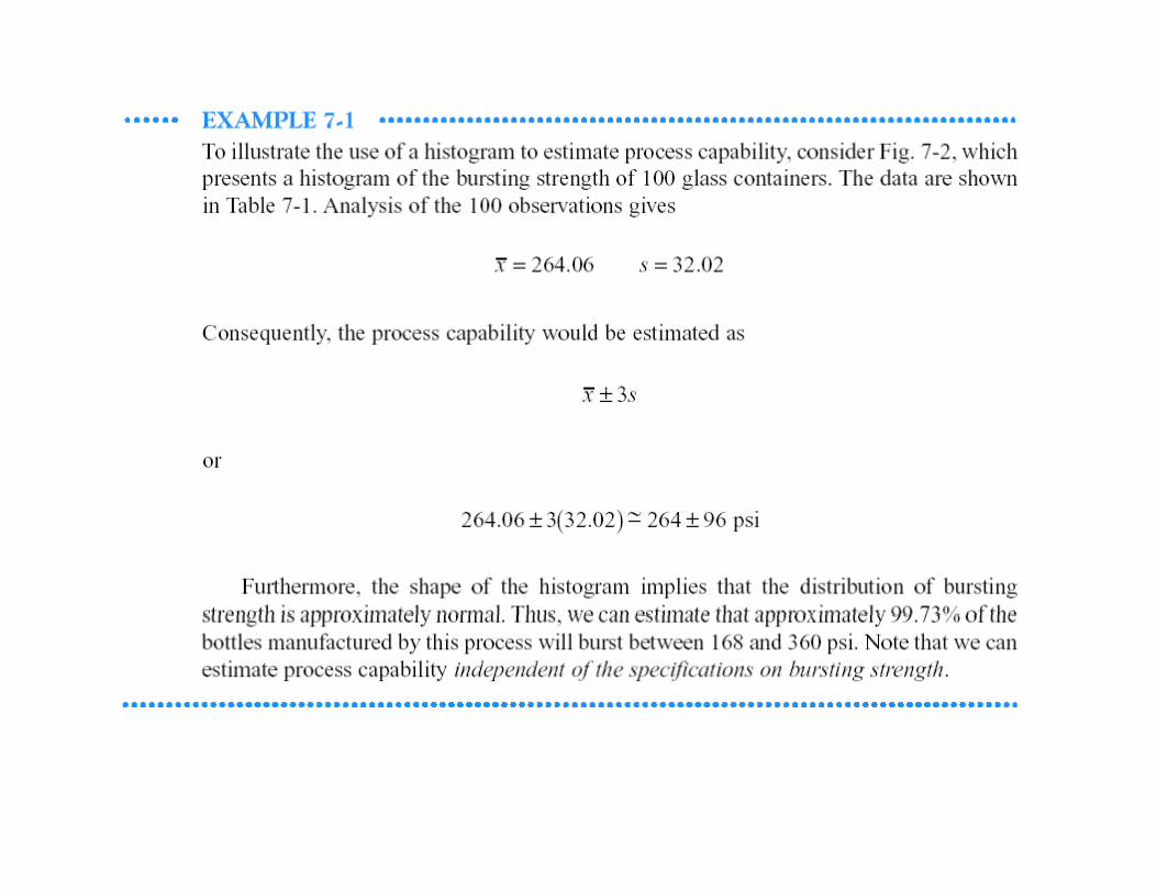
Example 7-1, Glass Container Data

Probability Plotting

Mean and standardstandard

deviation could be estimated from

the plotp

• The distribution may not be normal; other types of probability plots can be useful in determining the appropriate distribution.

Process Capability Ratios

Example 5-1: USL = 1.00 microns, LSL = 2.00 microns

0.1398Rd

σ = =2d

Practical interpretation

PCR = proportion of tolerance interval used by process

For the hard bake process:

One-Sided PCR

• Cp does not take process centering into accountaccount

• It is a measure of potential capability, not p p y,actual capability

Measure of Actual Capability

Cpk: one-sided PCR for specification limit nearest to process average

Normality and Process Capability Ratiosy p y

• The assumption of normality is critical to the interpretation of these ratios.p

• For non-normal data, options are:1. Transform non-normal data to normal.2 Extend the usual definitions of PCRs to handle non normal2. Extend the usual definitions of PCRs to handle non-normal

data.3. Modify the definitions of PCRs for general families of

distributions.d st but o s• Confidence intervals are an important way to express the information in a PCR

Confidence interval is wide because the sample size is smallp

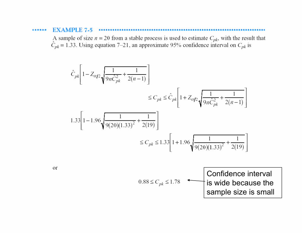
Confidence interval is wide because the

l i i llsample size is small

Process Performance Index:

Use only when the process is not in control.

If the process is normally distributed and in control:

ˆ ˆˆ ˆ R

2

ˆ and because p p pk pkRP C P Cd

σ= = ≈

Process Capability Analysis Using Control Chart

• Specifications are not needed to estimate parameters.

Since LSL = 200

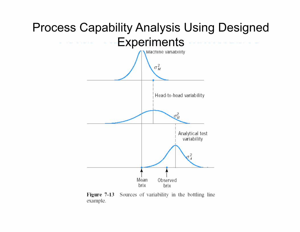
Process Capability Analysis Using Designed ExperimentsExperiments

Gauge and Measurement System Capability

Simple model:Simple model:

y: total observed measurementx: true value of measurementx: true value of measurementε: measurement error

( ) ( )2 2Gauge and are independent. , and 0, Px x N Nε µ σ ε σ∼ ∼( ) ( )GaugeP

k = 5.15 → number of standard deviation between 95% tolerance intervalContaining 99% of normal population.k 6 number of standard deviations between natural tolerance limit ofk = 6 → number of standard deviations between natural tolerance limit of normal population.

For Example 7-7, USL = 60 and LSL = 5. With k =6p

P/T ≤ 0.1 is taken as appropriate.

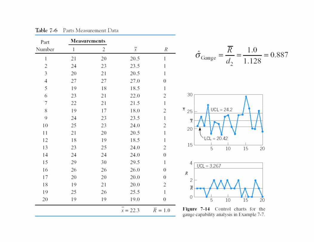
Estimating Variances

( )22GaugeˆBecause we estimate 0.887 0.79 :σ = =

→

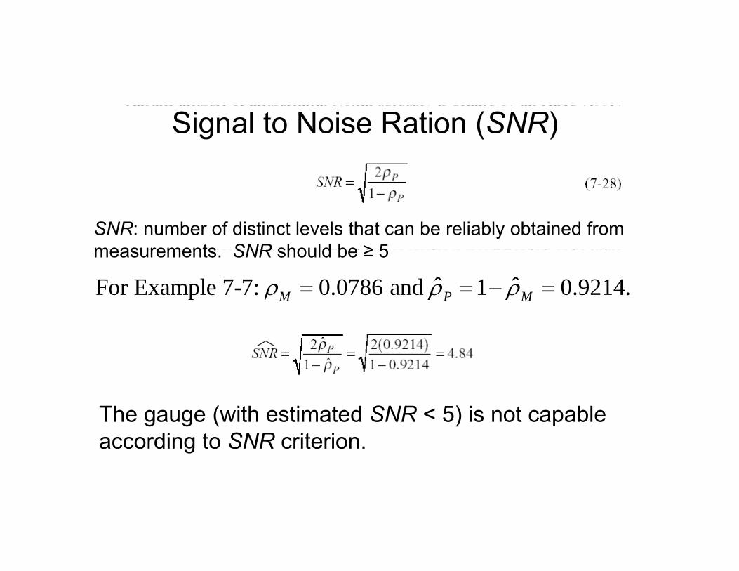
Signal to Noise Ration (SNR)

SNR: number of distinct levels that can be reliably obtained from measurements SNR should be ≥ 5measurements. SNR should be ≥ 5

ˆ ˆFor Example 7-7: 0.0786 and 1 0.9214.M P Mρ ρ ρ= = − =

The gauge (with estimated SNR < 5) is not capable according to SNR criterion.

Discrimination RatioDiscrimination Ratio

DR > 4 for capable gauges. p g gFor example, 7-7:

The gauge is capable according to DR criterion.

Gauge R&R Studies

• Usually conducted with a factorial experiment (p: number of randomly selected parts, o: number of randomly selected operators, n: number of times each operator measures each part)operators, n: number of times each operator measures each part)

( )( )

2

2

0, : effects of parts

0, : effects of operators

i P

j O

P N

O N

σ

σ

∼

∼ ( )( ) ( )

( )

2

2

0, : joint effects of parts and operators

0, : effects of operators

POij

ijk

PO N

N

σ

ε σ

∼

∼ ( )

• This is a two-factor factorial experiment.

• ANOVA methods are used to conduct the R&R analysis.

• Negative estimates of a variance component would lead to filling a reduced model such as for example:lead to filling a reduced model, such as, for example:

σ2: repeatability variance component

→→

For the example:For the example:

With LSL = 18 and USL = 58:

This gauge is not capable since P/T > 0.1.

Linear Combinations

( )2For assume and independent from each otherx x x x N µ σ( )1 2

1 1 2 2

2 2

For , , , , assume , and independent from each other.

Let ... .n i i i

n n

n n

x x x x N

y a x a x a x

µ σ

= + + +

⎛ ⎞∑ ∑

… ∼

2 2

1 1Then ,i i i i

i iy N a aµ σ

= =

⎛ ⎞∼ ⎜ ⎟

⎝ ⎠∑ ∑

Nonlinear Combinations

( ) li f i f( )

( )

1 2: nonlinear function of , , ,: nominal (i.e., average) dimension for (for 1, 2,... )

Taylor series expansion of :

n

i i

g x x xx i n

gµ

•

=

•

…

( )Taylor series expansion of :g •

→

R is higher order (2 or higher) remainder of the expansion.R → 0

→→

Assume I and R are centered at the nominal values.α = 0.0027: fraction of values falling outside the natural tolerance limits.S fSpecification limits are equal to natural tolerance limits.

( )2Assume 25 1 Amp or 24 26 and I 25, .

3 0II I N

Z Z

σ= ± ≤ ≤

= =

∼

/ 2 0.00135 3.026 25 3.0 0.33I

I

Z Zα

σσ

= =

−→ = → =

( )( )2Assume 4 0.06 ohms or 3.94 4.06 and I 4, .

4.06 4.00 3.0 0.02

R

RR

R I N σ

σσ

= ± ≤ ≤

−→ = → =

∼

Rσ

Assuming V is approximately normal:

→

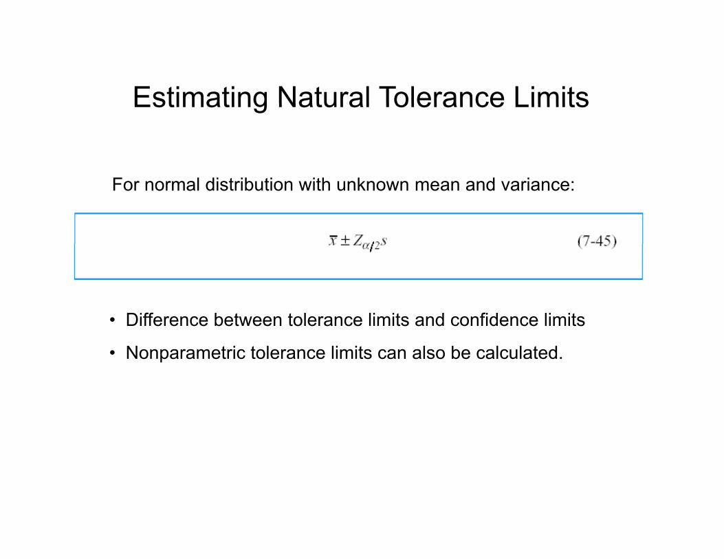
Estimating Natural Tolerance LimitsEstimating Natural Tolerance Limits

For normal distribution with unknown mean and variance:

Diff b t t l li it d fid li it• Difference between tolerance limits and confidence limits

• Nonparametric tolerance limits can also be calculated.