Embed Size (px)
Citation preview
1 Lecture Notes TTK 4190 Guidance and Control of Vehicles (T. I. Fossen)
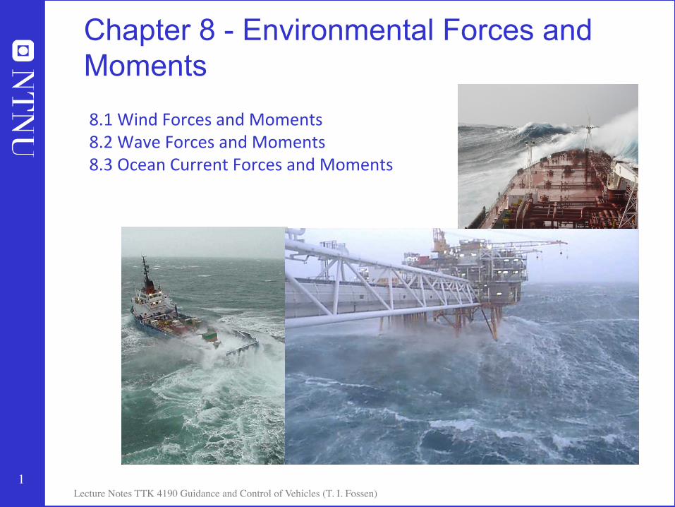
Chapter 8 - Environmental Forces and Moments 8.1 Wind Forces and Moments 8.2 Wave Forces and Moments 8.3 Ocean Current Forces and Moments
2 Lecture Notes TTK 4190 Guidance and Control of Vehicles (T. I. Fossen)
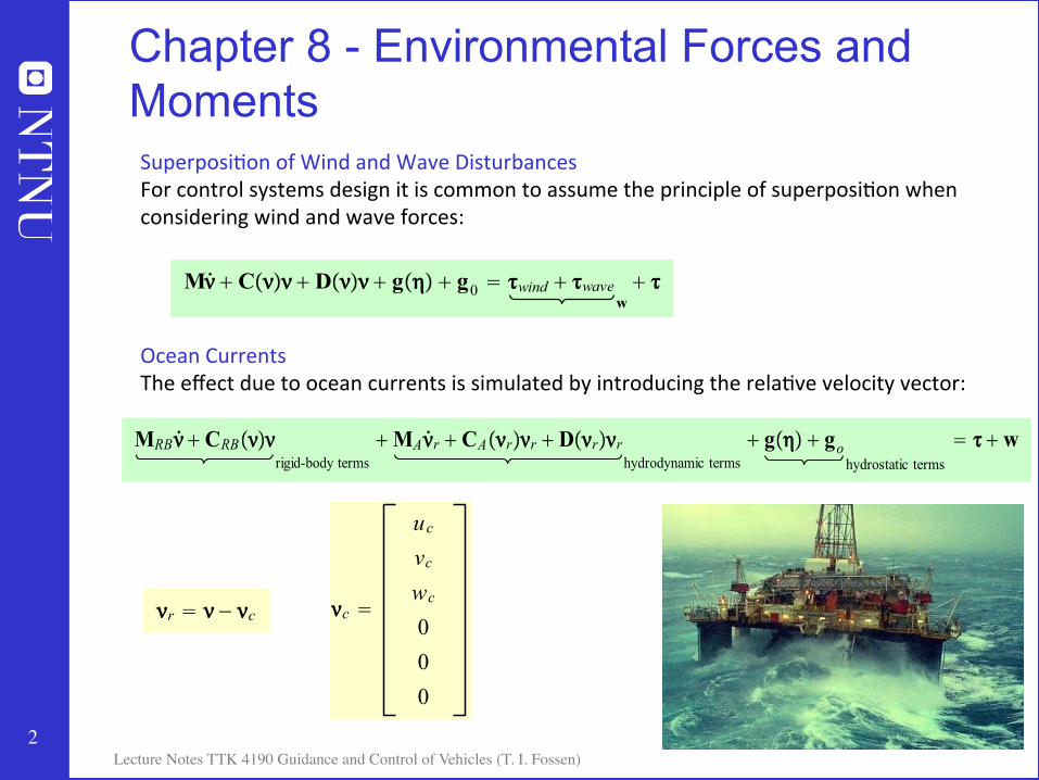
Superposi;on of Wind and Wave Disturbances For control systems design it is common to assume the principle of superposi;on when considering wind and wave forces: Ocean Currents The effect due to ocean currents is simulated by introducing the rela;ve velocity vector:
Chapter 8 - Environmental Forces and Moments
M !! " C!!"! " D!!"! " g!"" " g0 # #wind " #wavew" # #
!r ! ! ! !c # !c !
ucvcwc000
MRB !! " CRB!!"!rigid-body terms
"MA !!r " CA!!r"!r " D!!r"!rhydrodynamic terms
" g!"" " gohydrostatic terms
# # " w #
3 Lecture Notes TTK 4190 Guidance and Control of Vehicles (T. I. Fossen)
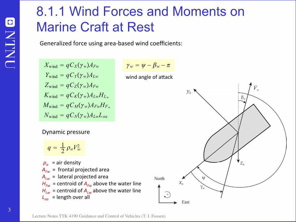
Dynamic pressure ρa = air density AFw = frontal projected area ALw = lateral projected area HFw = centroid of AFw above the water line HLw = centroid of ALw above the water line Loa = length over all
Generalized force using area-‐based wind coefficients:
8.1.1 Wind Forces and Moments on Marine Craft at Rest
Xwind ! qCX!!w"AFwYwind ! qCY!!w"ALwZwind ! qCZ!!w"AFwKwind ! qCK!!w"ALwHLwMwind ! qCM!!w"AFwHFwNwind ! qCN!!w"ALwLoa
# # # # # #
q ! 12 !aVw2 #
!w ! " ! #w ! $ #
wind angle of aMack
4 Lecture Notes TTK 4190 Guidance and Control of Vehicles (T. I. Fossen)
8.1.1 Wind Forces and Moments on Marine Craft at Rest
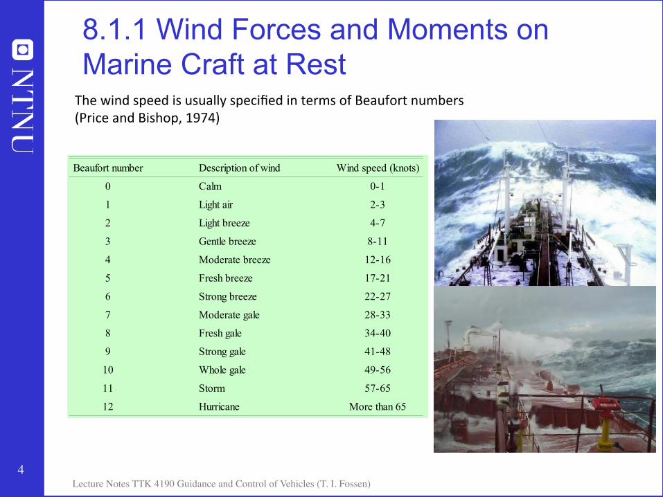
Beaufort number Description of wind Wind speed (knots)
0 Calm 0-1
1 Light air 2-3
2 Light breeze 4-7
3 Gentle breeze 8-11
4 Moderate breeze 12-16
5 Fresh breeze 17-21
6 Strong breeze 22-27
7 Moderate gale 28-33
8 Fresh gale 34-40
9 Strong gale 41-48
10 Whole gale 49-56
11 Storm 57-65
12 Hurricane More than 65
The wind speed is usually specified in terms of Beaufort numbers (Price and Bishop, 1974)

5 Lecture Notes TTK 4190 Guidance and Control of Vehicles (T. I. Fossen)
8.1.1 Wind Forces and Moments on Marine Craft at Rest Wind Coefficient Approxima;on for Symmetrical Ships For ships that are symmetrical with respect to the xz-‐ and yz-‐planes, the wind coefficients for horizontal-‐plane mo;ons can be approximated by: which are convenient formulae for computer simula;ons. Experiments indicate that:
cx ∈ {0.50, 0.90} cy ∈ {0.70, 0.95} cn ∈ {0.05, 0.20}
These values should be used with care.
CX!!w" ! "cx cos!!w"CY!!w" ! cy sin!!w"CN!!w" ! cn sin!2!w"
# # #
6 Lecture Notes TTK 4190 Guidance and Control of Vehicles (T. I. Fossen)
8.1.2 Wind Forces and Moments on Moving Marine Craft
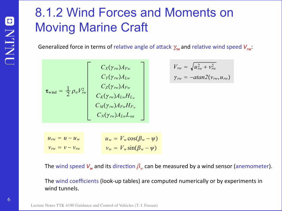
!wind ! 12 !aVrw2
CX!"rw"AFwCY!"rw"ALwCZ!"rw"AFw
CK!"rw"ALwHLwCM!"rw"AFwHFwCN!"rw"ALwLoa
#
Vrw ! urw2 " vrw2
!rw ! !atan2!vrw,urw"
#
#
urw ! u ! uwvrw ! v ! vrw
# #
uw ! Vw cos!!w ! ""
vw ! Vw sin!!w ! ""
# #
The wind speed Vw and its direc;on βw can be measured by a wind sensor (anemometer). The wind coefficients (look-‐up tables) are computed numerically or by experiments in wind tunnels.
Generalized force in terms of rela;ve angle of aMack γrw and rela;ve wind speed Vrw:

7 Lecture Notes TTK 4190 Guidance and Control of Vehicles (T. I. Fossen)
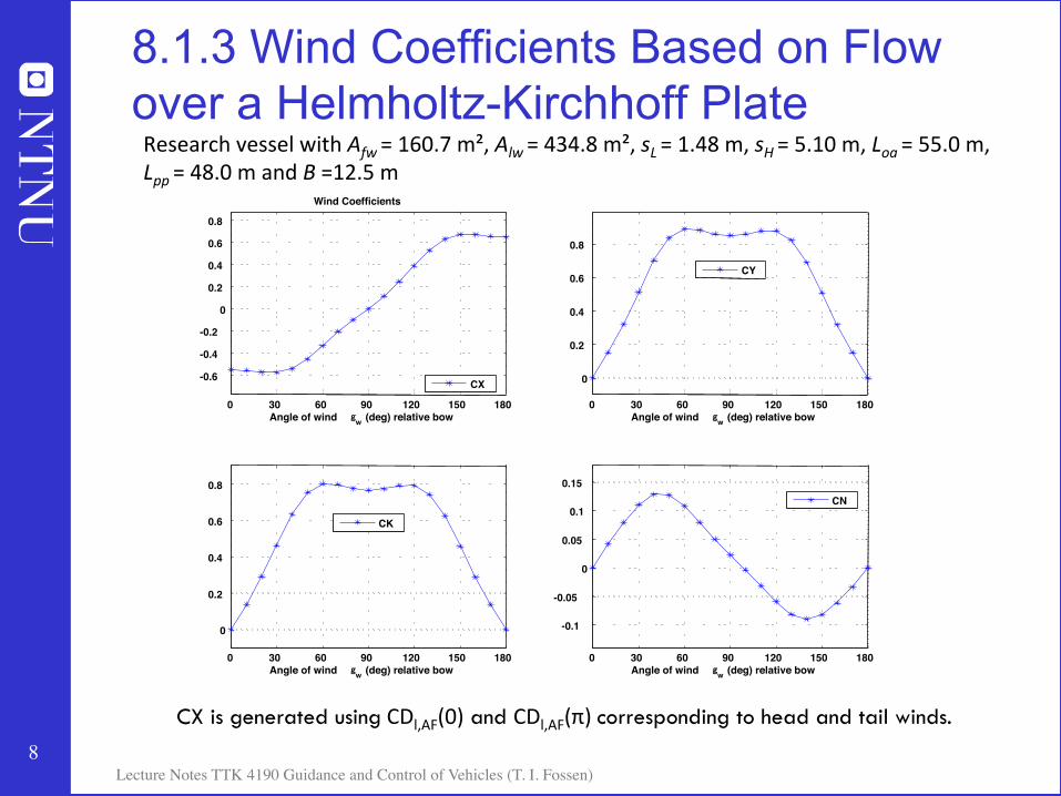
8.1.3 Wind Coefficients Based on Flow over a Helmholtz-Kirchhoff Plate
Reference: Blendermann (1994) The load func;ons are parameterized in terms of four primary wind load parameters:
CX!!w" ! !CDlALwAFw
CDlAF
cos!!w"1 ! "
2 1 ! CDlCDt
sin2!2!w"
CY!!w" ! CDtsin!!w"
1 ! "2 1 ! CDl
CDtsin2!2!w"
CK!!w" ! #CY!!w"
CN!!w" ! sLLoa ! 0.18 !w ! $
2 CY!!w"
#
#
#
#
Type of vessel CDt CDlAF!0" CDlAF!!" " #
1. Car carrier 0.95 0.55 0.60 0.80 1.2
2. Cargo vessel, loaded 0.85 0.65 0.55 0.40 1.7
3. Cargo vessel, container on deck 0.85 0.55 0.50 0.40 1.4
4. Container ship, loaded 0.90 0.55 0.55 0.40 1.4
5. Destroyer 0.85 0.60 0.65 0.65 1.1
6. Diving support vessel 0.90 0.60 0.80 0.55 1.7
7. Drilling vessel 1.00 0.70–1.00 0.75–1.10 0.10 1.7
8. Ferry 0.90 0.45 0.50 0.80 1.1
9. Fishing vessel 0.95 0.70 0.70 0.40 1.1
10. Liquified natural gas tanker 0.70 0.60 0.65 0.50 1.1
11. Offshore supply vessel 0.90 0.55 0.80 0.55 1.2
12. Passenger liner 0.90 0.40 0.40 0.80 1.2
13. Research vessel 0.85 0.55 0.65 0.60 1.4
14. Speed boat 0.90 0.55 0.60 0.60 1.1
15. Tanker, loaded 0.70 0.90 0.55 0.40 3.1
16. Tanker, in ballast 0.70 0.75 0.55 0.40 2.2
17. Tender 0.85 0.55 0.55 0.65 1.1
CDl ! CDlAF !!w"AFwALw
#
Matlab MSS toolbox >> [w_wind,CX,CY,CK,CN] = blendermann94(gamma_r,V_r,AFw,ALw,sH,sL,Loa,vessel_no)
8 Lecture Notes TTK 4190 Guidance and Control of Vehicles (T. I. Fossen)
0 30 60 90 120 150 180 -0.6 -0.4 -0.2
0 0.2 0.4 0.6 0.8
Angle of wind g w (deg) relative bow
Wind Coefficients
0 30 60 90 120 150 180 0
0.2 0.4 0.6 0.8
Angle of wind g w (deg) relative bow
0 30 60 90 120 150 180 0
0.2 0.4 0.6 0.8
Angle of wind g w (deg) relative bow
0 30 60 90 120 150 180 -0.1
-0.05 0
0.05 0.1
0.15
Angle of wind g w (deg) relative bow
CX
CY
CK CN
8.1.3 Wind Coefficients Based on Flow over a Helmholtz-Kirchhoff Plate
CX is generated using CDl,AF(0) and CDl,AF(π) corresponding to head and tail winds.
Research vessel with Afw = 160.7 m², Alw = 434.8 m², sL = 1.48 m, sH = 5.10 m, Loa = 55.0 m, Lpp = 48.0 m and B =12.5 m
9 Lecture Notes TTK 4190 Guidance and Control of Vehicles (T. I. Fossen)
8.1.4 – 8.1.7 Wind Coefficients
8.1.4 Wind Coefficients for Merchant Ships (Isherwood, 1972) Isherwood (1972) has derived a set of wind coefficients by using mul;ple regression techniques to fit experimental data of merchant ships. The wind coefficients are parameterized in terms of eight parameters. 8.1.5 Wind Resistance of Very Large Crude Carriers (OCIMF, 1977) Wind loads on very large crude carriers (VLCCs) in the range 150 000 to 500 000 dwt can be computed by applying the results of (OCIMF 1977). 8.1.6 Wind Resistance of Large Tankers and Medium Sized Ships For wind resistance on large tankers in the 100 000 to 500 000 dwt class the reader is advised to consult Van Berlekom et al. (1974). Medium sized ships of the order 600 to 50 000 dwt is discussed by Wagner (1967). 8.1.7 Wind Resistance of Moored Ships and Floa;ng Structures Wind loads on moored ships are discussed by De Kat and Wichers (1991) while an excellent reference for huge pontoon type floa;ng structures is Kitamura et al. (1997).

10 Lecture Notes TTK 4190 Guidance and Control of Vehicles (T. I. Fossen)
8.2 Wave Forces and Moments A marine control system can be simulated under influence of wave-‐induced forces by separa;ng the 1st-‐order and 2nd-‐order effects:
• 1st-‐order wave-‐induced forces (wave-‐frequency mo6on) Zero-‐mean oscillatory mo;ons • 2nd-‐order wave-‐induced forces (wave dri9 forces) Nonzero slowly varying component
Wave forces are observed as a mean slowly varying component referred to as Low-‐ Frequency (LF) mo;ons and an oscillatory component called Wave-‐Frequency (WF) mo;ons which must be compensated for by the feedback control system: • The mean component (LF) can be removed
by using integral ac;on
• The oscillatory component (WF) is usually removed by using a cascaded notch and low-‐pass filter (wave filtering)
!wave ! !wave1 " !wave2 #
11 Lecture Notes TTK 4190 Guidance and Control of Vehicles (T. I. Fossen)
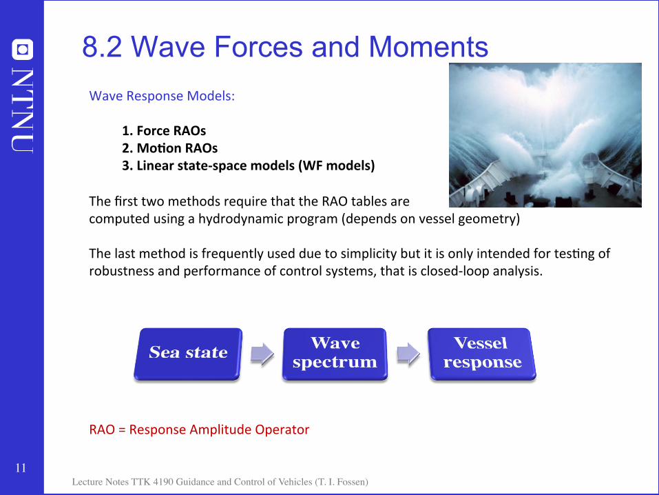
8.2 Wave Forces and Moments Wave Response Models:
1. Force RAOs 2. Mo6on RAOs 3. Linear state-‐space models (WF models)
The first two methods require that the RAO tables are computed using a hydrodynamic program (depends on vessel geometry) The last method is frequently used due to simplicity but it is only intended for tes;ng of robustness and performance of control systems, that is closed-‐loop analysis. RAO = Response Amplitude Operator
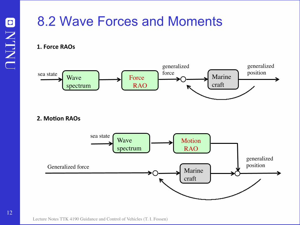
12 Lecture Notes TTK 4190 Guidance and Control of Vehicles (T. I. Fossen)
1. Force RAOs 2. Mo6on RAOs
8.2 Wave Forces and Moments
Marine craft
Wave spectrum
sea state generalized force
generalized position
Marine craft
Wave spectrum
sea state
Generalized force generalized position
Force RAO
Motion RAO

13 Lecture Notes TTK 4190 Guidance and Control of Vehicles (T. I. Fossen)
8.2 Wave Forces and Moments 3. Linear State-‐Space Models (WF models)
Marine craft
Linear wave spectrum approximation
White noise
Generalized force generalized position
Tunable gain K
WF position

14 Lecture Notes TTK 4190 Guidance and Control of Vehicles (T. I. Fossen)
8.2 Wave Forces and Moments 1. Force RAOs 2. Mo6on RAOs 3. Linear state-‐space models (WF models)
Wavespectrum Motion RAO
Seastate
Waveamplitude
1st-order wave-induced positions
S( )ω
ηwH ,Ts z Ak
Wavespectrum
1st-orderForce RAO
Seastate
Waveamplitude
1st-order wave-induced force
2nd-orderForce RAO
2nd-order wave drift force
S( )ω
τwave1H ,Ts z Ak
Generalized force
Generalized posi;on
Generalized posi;on

15 Lecture Notes TTK 4190 Guidance and Control of Vehicles (T. I. Fossen)
8.2.1 Sea State Descriptions For marine crai the sea can be characterized by the following wave spectrum parameters:
• The significant wave height Hs (the mean wave height of the one third highest waves, also denoted as H1/3) • One of the following wave periods:
-‐ The average wave period, T₁ -‐ Average zero-‐crossing wave period, Tz -‐ Peak period, Tp (this is equivalent to the modal period, T₀)
16 Lecture Notes TTK 4190 Guidance and Control of Vehicles (T. I. Fossen)
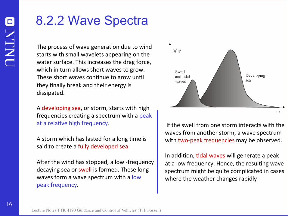
8.2.2 Wave Spectra
The process of wave genera;on due to wind starts with small wavelets appearing on the water surface. This increases the drag force, which in turn allows short waves to grow. These short waves con;nue to grow un;l they finally break and their energy is dissipated. A developing sea, or storm, starts with high frequencies crea;ng a spectrum with a peak at a rela;ve high frequency. A storm which has lasted for a long ;me is said to create a fully developed sea. Aier the wind has stopped, a low -‐frequency decaying sea or swell is formed. These long waves form a wave spectrum with a low peak frequency.
S( )ω
Swelland tidalwaves
Developingsea
ω
If the swell from one storm interacts with the waves from another storm, a wave spectrum with two-‐peak frequencies may be observed. In addi;on, ;dal waves will generate a peak at a low frequency. Hence, the resul;ng wave spectrum might be quite complicated in cases where the weather changes rapidly
17 Lecture Notes TTK 4190 Guidance and Control of Vehicles (T. I. Fossen)
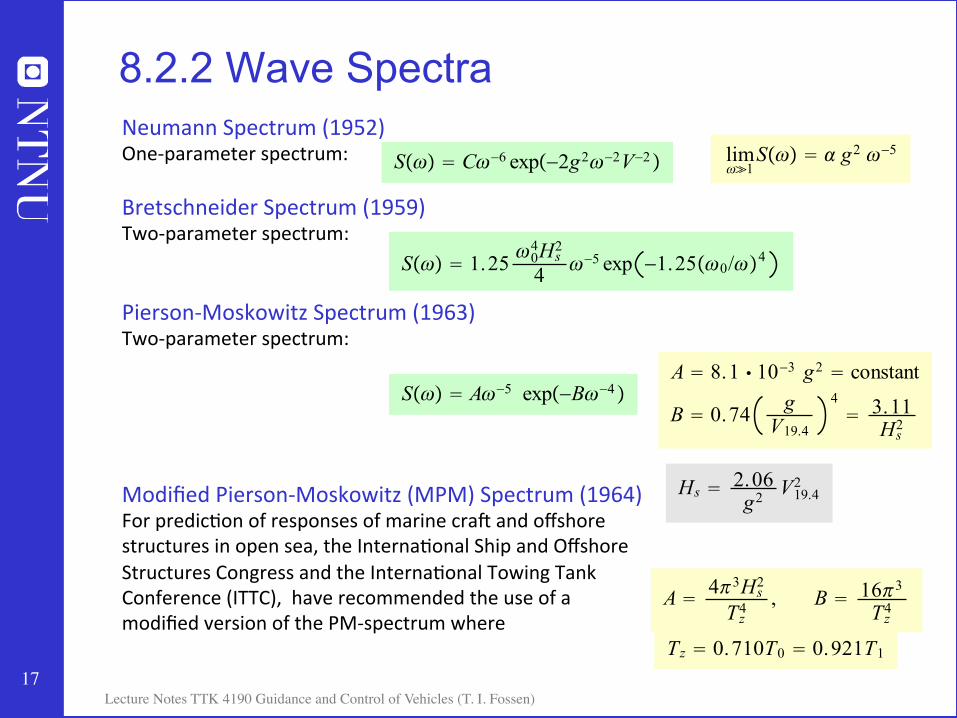
8.2.2 Wave Spectra Neumann Spectrum (1952) One-‐parameter spectrum: Bretschneider Spectrum (1959) Two-‐parameter spectrum: Pierson-‐Moskowitz Spectrum (1963) Two-‐parameter spectrum: Modified Pierson-‐Moskowitz (MPM) Spectrum (1964) For predic;on of responses of marine crai and offshore structures in open sea, the Interna;onal Ship and Offshore Structures Congress and the Interna;onal Towing Tank Conference (ITTC), have recommended the use of a modified version of the PM-‐spectrum where
A ! 8.1 ! 10!3 g2 ! constant
B ! 0.74 gV19.4
4! 3.11
Hs2
#
# S!!" ! A!!5 exp!!B!!4" #
S!!" ! 1.25 !04Hs24 !!5 exp !1.25!!0/!"4 #
S!!" ! C!!6 exp!!2g2!!2V!2" # lim!!1S!!" ! " g2 !"5 #
Hs ! 2.06g2 V19.4
2 #
A ! 4!3Hs2Tz4
, B ! 16!3
Tz4 #
Tz ! 0.710T0 ! 0.921T1 #
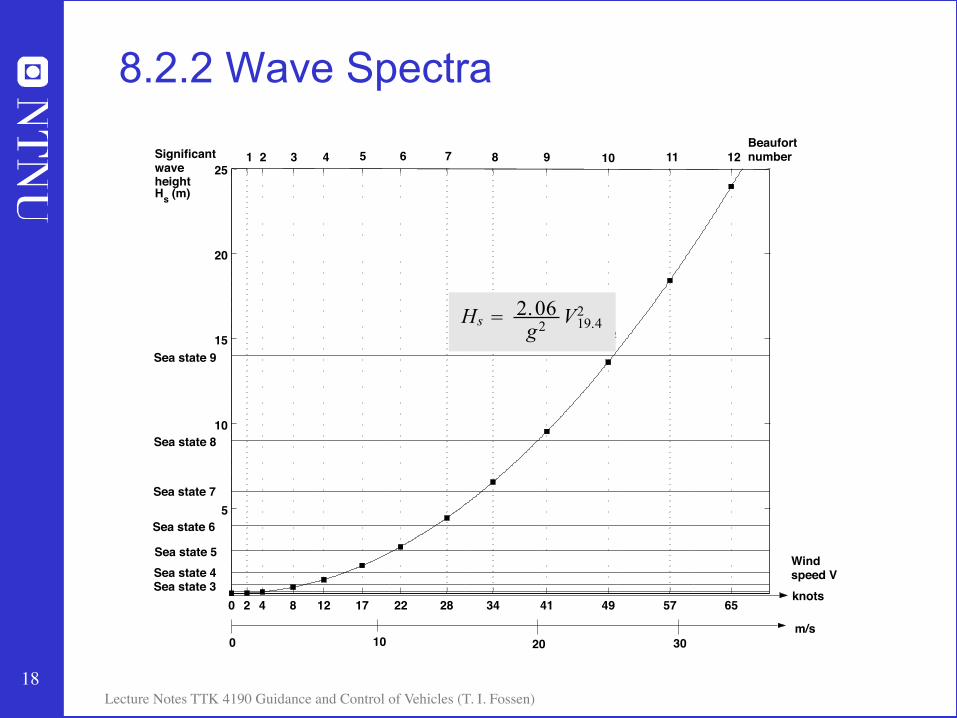
18 Lecture Notes TTK 4190 Guidance and Control of Vehicles (T. I. Fossen)
0 2 4 8 12 17 22 28 34 41 49 57 65
5
10
15
20
25
knots m/s
Sea state 9
Sea state 8
Sea state 7 Sea state 6 Sea state 5 Sea state 4 Sea state 3
Significant wave height H s (m)
30 20 10 0
Wind speed V
Beaufort number 1 2 3 4 5 6 7 8 9 10 12 11
H s = 2.06 V 2 /g 2
8.2.2 Wave Spectra
Hs ! 2.06g2 V19.4
2 #
19 Lecture Notes TTK 4190 Guidance and Control of Vehicles (T. I. Fossen)
8.2.2 Wave Spectra
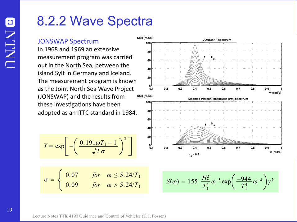
S!!" ! 155 Hs2T1
4 !!5 exp !944T1
4 !!4 "Y # ! !0.07 for " ! 5.24/T1
0.09 for " " 5.24/T1 #
0.1 0.2 0.3 0.4 0.5 0.6 0.7 0.8 0.9 1 0 20 40 60 80
100 JONSWAP spectrum
w (rad/s)
0.1 0.2 0.3 0.4 0.5 0.6 0.7 0.8 0.9 1 0 20 40 60 80
100 Modified Pierson-Moskowitz (PM) spectrum
w (rad/s) w
o = 0.4
H s
H s
S( w ) (rad/s)
S( w ) (rad/s)
JONSWAP Spectrum In 1968 and 1969 an extensive measurement program was carried out in the North Sea, between the island Sylt in Germany and Iceland. The measurement program is known as the Joint North Sea Wave Project (JONSWAP) and the results from these inves;ga;ons have been adopted as an ITTC standard in 1984.
Y ! exp ! 0.191!T1 ! 12 "
2
#
20 Lecture Notes TTK 4190 Guidance and Control of Vehicles (T. I. Fossen)
8.2.2 Wave Spectra
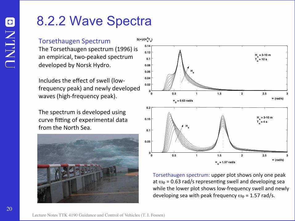
Torsethaugen spectrum: upper plot shows only one peak at ω₀ = 0.63 rad/s represen;ng swell and developing sea while the lower plot shows low-‐frequency swell and newly developing sea with peak frequency ω₀ = 1.57 rad/s.
0 0.5 1 1.5 2 2.5 3 0 0.02 0.04 0.06 0.08
0.1 0.12 0.14
w (rad/s)
0 0.5 1 1.5 2 2.5 3 0 0.05
0.1 0.15
0.2
w (rad/s)
H s = 3-10 m T o = 10 s
H s = 3-10 m T o = 4 s
S( w )/(H s 2 T o )
H s
H s
w 0 = 0.63 rad/s
w o = 1.57 rad/s
Torsethaugen Spectrum The Torsethaugen spectrum (1996) is an empirical, two-‐peaked spectrum developed by Norsk Hydro. Includes the effect of swell (low-‐frequency peak) and newly developed waves (high-‐frequency peak). The spectrum is developed using curve fimng of experimental data from the North Sea.
21 Lecture Notes TTK 4190 Guidance and Control of Vehicles (T. I. Fossen)
8.2.2 Wave Spectra
0 0.2 0.4 0.6 0.8 1 1.2 1.4 1.6 1.8 2 0
0.005
0.01
0.015
0.02
0.025
0.03
0.035
0.04
w (rad/s)
S( w )/(H s 2 T 0 )
Modified Pierson-Moskowitz JONSWAP for g = 3.3 JONSWAP for g = 2.0 Torsethaugen
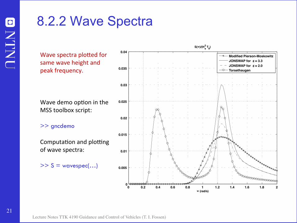
Wave spectra ploMed for same wave height and peak frequency. Wave demo op;on in the MSS toolbox script: >> gncdemo Computa;on and plomng of wave spectra: >> S = wavespec(…)
22 Lecture Notes TTK 4190 Guidance and Control of Vehicles (T. I. Fossen)
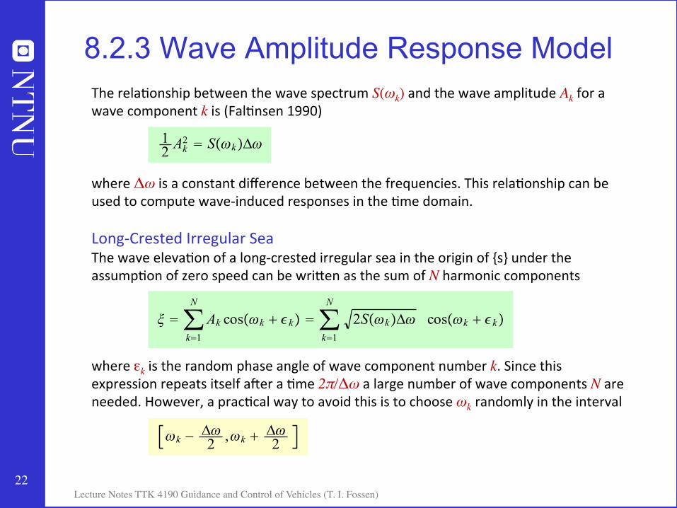
8.2.3 Wave Amplitude Response Model The rela;onship between the wave spectrum S(ωk) and the wave amplitude Ak for a wave component k is (Fal;nsen 1990) where Δω is a constant difference between the frequencies. This rela;onship can be used to compute wave-‐induced responses in the ;me domain. Long-‐Crested Irregular Sea The wave eleva;on of a long-‐crested irregular sea in the origin of {s} under the assump;on of zero speed can be wriMen as the sum of N harmonic components where εk is the random phase angle of wave component number k. Since this expression repeats itself aier a ;me 2π/Δω a large number of wave components N are needed. However, a prac;cal way to avoid this is to choose ωk randomly in the interval
12 Ak
2 ! S!!k""! #
! ! !k!1
N
Ak cos!"k " #k" ! !k!1
N
2S!"k"#" cos!"k " #k" #
!k ! !!2 ,!k " !!
2 #

23 Lecture Notes TTK 4190 Guidance and Control of Vehicles (T. I. Fossen)
8.2.3 Wave Amplitude Response Model Short-‐Crested Irregular Sea The most likely situa;on encountered at sea is short crested or confused waves. This is observed as irregulari;es along the wave crest at right angles to the direc;on of the wind. Short-‐crested irregular sea can be modeled by a 2-‐D wave spectrum where β = 0 corresponds to the main wave propaga;on direc;on while a nonzero β-‐value will spread the energy at different direc;ons.
S!!,"" ! S!!"f!"" #
f!!" !2" cos2!!", ! "/2 " ! " "/2
0; elsewhere #
! ! !k!1
N
!i!1
M
2S!"k ,#i""""# cos!"k # $k" #
Spreading func;on
Wave eleva;on
24 Lecture Notes TTK 4190 Guidance and Control of Vehicles (T. I. Fossen)
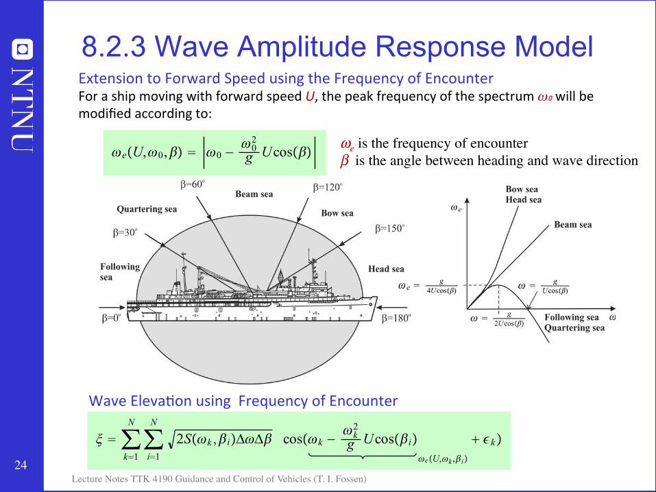
8.2.3 Wave Amplitude Response Model Extension to Forward Speed using the Frequency of Encounter For a ship moving with forward speed U, the peak frequency of the spectrum ω₀ will be modified according to:
!e!U,!0,"" ! !0 !!0
2
g Ucos!"" #
! ! !k!1
N
!i!1
N
2S!"k ,#i""""# cos!"k ""k
2
g Ucos!#i""e!U,"k ,#i"
# $k" #
Wave Eleva;on using Frequency of Encounter
ωe is the frequency of encounter β is the angle between heading and wave direction
25 Lecture Notes TTK 4190 Guidance and Control of Vehicles (T. I. Fossen)
Normalized Force RAOs The 1st-‐ and 2nd-‐order wave forces for varying wave direc;ons βi and wave frequencies ωk Processing Re-‐Im parts of the RAOs (ASCII file generated by hydrodynamic code)
8.2.4 Wave Force Response Amplitude Operators
Fwave1!dof" #!k ,"i$ !
#"wave1!dof" #!k ,"i$
$gAkej!#"wave1
!dof" #!k ,"i$
Fwave2!dof" #!k ,"i$ !
#"wave2!dof" #!k ,"i$
$gAk2ej!#"wave2
!dof" #!k ,"i$
#
#
Fwave1!dof" #!k ,"i$ ! Imwave1!dof"#k, i$2 " Rewave1!dof"#k, i$2
!Fwave1!dof" #!k ,"i$ ! atan#Imwave1!dof"#k, i$,Rewave1!dof"#k, i$$
#
#
Fwave2!dof" #!k ,"i$ ! Rewave2!dof"#k, i$
!Fwave2!dof" #!k ,"i$ ! 0
#
#
complex variables
(wave drii)

26 Lecture Notes TTK 4190 Guidance and Control of Vehicles (T. I. Fossen)
No Spreading Func;on With Spreading Func;on
8.2.4 Wave Force Response Amplitude Operators
!wave1!dof" ! !
k!1
N
"g Fwave1!dof" ##k ,$$ Ak cos #e#U,#k ,$$t " "Fwave1
!dof" ##k ,$$ " %k
!wave2!dof" ! !
k!1
N
"g Fwave2!dof" ##k ,$$ Ak2 cos##e#U,#k ,$$t " %k $
#
# (wave drii)
Wavespectrum
1st-orderForce RAO
Seastate
Waveamplitude
1st-order wave-induced force
2nd-orderForce RAO
2nd-order wave drift force
S( )ω
τwave1H ,Ts z Ak 1
2 Ak2 ! S!!k""! #
!wave1!dof" ! !
k!1
N
!i!1
M
"g Fwave1!dof" ##k ,$i$ Ak cos #e#U,#k ,$i$t " "Fwave1
!dof" ##k ,$i$ " %k
!wave2!dof" ! !
k!1
N
!i!1
M
"g Fwave2!dof" ##k ,$i$ Ak2 cos##e#U,#k ,$i$t " %k $
#
# (wave drii)
27 Lecture Notes TTK 4190 Guidance and Control of Vehicles (T. I. Fossen)
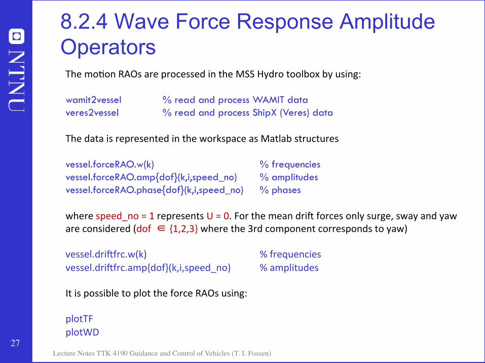
8.2.4 Wave Force Response Amplitude Operators The mo;on RAOs are processed in the MSS Hydro toolbox by using: wamit2vessel % read and process WAMIT data veres2vessel % read and process ShipX (Veres) data The data is represented in the workspace as Matlab structures vessel.forceRAO.w(k) % frequencies vessel.forceRAO.amp{dof}(k,i,speed_no) % amplitudes vessel.forceRAO.phase{dof}(k,i,speed_no) % phases where speed_no = 1 represents U = 0. For the mean drii forces only surge, sway and yaw are considered (dof ∈ {1,2,3} where the 3rd component corresponds to yaw) vessel.driifrc.w(k) % frequencies vessel.driifrc.amp{dof}(k,i,speed_no) % amplitudes It is possible to plot the force RAOs using: plotTF plotWD
28 Lecture Notes TTK 4190 Guidance and Control of Vehicles (T. I. Fossen)
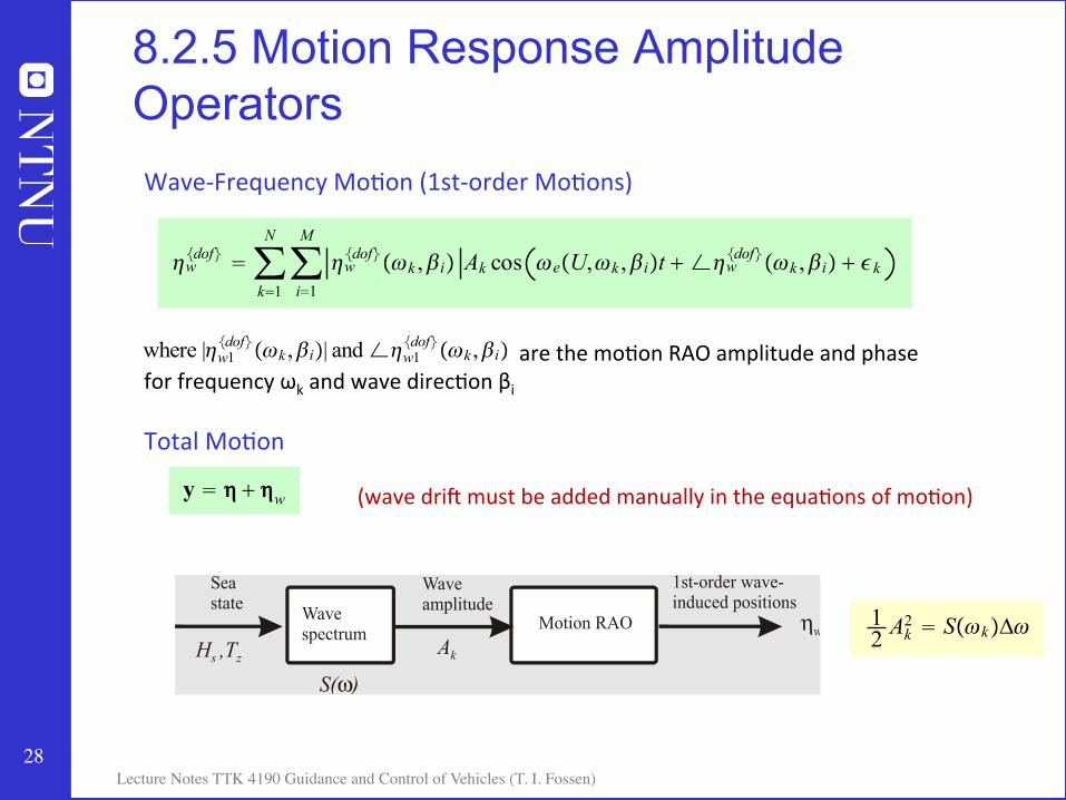
Wave-‐Frequency Mo;on (1st-‐order Mo;ons) are the mo;on RAO amplitude and phase for frequency ωk and wave direc;on βi Total Mo;on
8.2.5 Motion Response Amplitude Operators
(wave drii must be added manually in the equa;ons of mo;on)
12 Ak
2 ! S!!k""! #
!w!dof" ! !k!1
N
!i!1
M
!w!dof"#"k ,#i$ Ak cos "e#U,"k ,#i$t " "!w!dof"#"k ,#i$ " $k #
Wavespectrum Motion RAO
Seastate
Waveamplitude
1st-order wave-induced positions
S( )ω
ηwH ,Ts z Ak
y ! ! " !w #
where |!w1!dof"#"k ,#i$| and!!w1
!dof"#"k ,#i$
29 Lecture Notes TTK 4190 Guidance and Control of Vehicles (T. I. Fossen)
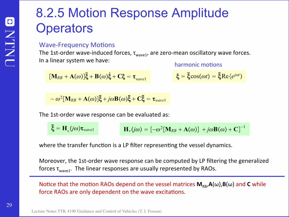
8.2.5 Motion Response Amplitude Operators Wave-‐Frequency Mo;ons The 1st-‐order wave-‐induced forces, τwave1, are zero-‐mean oscillatory wave forces. In a linear system we have: The 1st-‐order wave response can be evaluated as: where the transfer func;on is a LP filter represen;ng the vessel dynamics. Moreover, the 1st-‐order wave response can be computed by LP filtering the generalized forces τwave1. The linear responses are usually represented by RAOs. No;ce that the mo;on RAOs depend on the vessel matrices MRB,A(ω),B(ω) and C while force RAOs are only dependent on the wave excita;ons.
!MRB ! A"!#$!" ! B"!#!# ! C! " $wave1 # ! ! !" cos!!t" ! !"Re#ej!t" #
! !2!MRB ! A"!#$!" ! j!B"!#!" ! C!" " #wave1 #
!" ! Hv!j!"#wave1 # Hv!j!" ! #!!2#MRB " A!!"$ " j!B!!" " C$!1 #
harmonic mo;ons

30 Lecture Notes TTK 4190 Guidance and Control of Vehicles (T. I. Fossen)
8.2.6 State-Space Models for Wave Responses
!" ! J!!"#M "# # C!#"# # D!#"# # g!!" # g0 ! $wind # $wave2 # $
y ! ! # !w
# # # !w ! KHs!s"w!s" #
Approxima;on 2 (Wave Spectrum) A linear wave response approxima;on for Hs(s) is usually preferred by ship control systems engineers. Easy to use and easy to test control systems. No hydrodynamic SW is needed for the price of a tunable gain K which must be tuned manually to match the response ηw
Approxima;on 1 (WF Posi;on)
“tunable gain”

31 Lecture Notes TTK 4190 Guidance and Control of Vehicles (T. I. Fossen)
8.2.6 State-Space Models for Wave Responses
x! w1
x! w2"
0 1!!0
2 !2"!0
xw1
xw2#
0Kw
w #
yw ! 0 1xw1
xw2 #
h!s" ! Kwss2 " 2!"0s " "0
2 #
x! w ! Awxw " ewwyw!cw!xw
# #
Linear Wave Spectrum Approxima;on (Balchen 1976) PM-‐spectrum State-‐Space Model
S!!" ! A!!5 exp!!B!!4" #
32 Lecture Notes TTK 4190 Guidance and Control of Vehicles (T. I. Fossen)
8.2.6 State-Space Models for Wave Responses
33 Lecture Notes TTK 4190 Guidance and Control of Vehicles (T. I. Fossen)
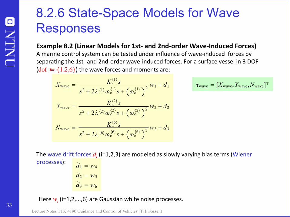
8.2.6 State-Space Models for Wave Responses Example 8.2 (Linear Models for 1st-‐ and 2nd-‐order Wave-‐Induced Forces) A marine control system can be tested under influence of wave-‐induced forces by separa;ng the 1st-‐ and 2nd-‐order wave-‐induced forces. For a surface vessel in 3 DOF (dof ∈ {1,2,6}) the wave forces and moments are: The wave drii forces di (i=1,2,3) are modeled as slowly varying bias terms (Wiener processes):
!wave ! !Xwave,Ywave,Nwave"! # Xwave ! Kw!1"ss2 " 2!!1""e!1"s " "e!1"
2 w1 " d1
Ywave ! Kw!2"ss2 " 2!!2""e!2"s " "e!2"
2 w2 " d2
Nwave ! Kw!6"ss2 " 2!!6""e!6"s " "e!6"
2 w3 " d3
#
#
#
d! 1 " w4d! 2 " w5d! 3 " w6
# # #
Here wi (i=1,2,...,6) are Gaussian white noise processes.

34 Lecture Notes TTK 4190 Guidance and Control of Vehicles (T. I. Fossen)
8.3 Ocean Current Forces and Moments Current Speed and Direc;on The current speed is denoted by Vc while its direc;on rela;ve to the moving crai is conveniently expressed in terms of two angles: angle of aMack αc, and sideslip angle βc For computer simula;ons the current velocity can be generated by using a 1st-‐order Gauss-‐Markov Process
V! c " !Vc # w # Vmin ! Vc!t" ! Vmax #
xb α-β
xstabzb
yb
Uxflow

35 Lecture Notes TTK 4190 Guidance and Control of Vehicles (T. I. Fossen)
8.3 Ocean Current Forces and Moments Equa;ons of Mo;on including Ocean Currents
rigid-‐body and hydrosta;c terms hydrodynamic terms
MRB !! " CRB!!"! " g!"" " g0 "MA !!r " CA!!r"!r " D!!r"!r # #wind " #wave " # #
!r ! ! ! !c rela;ve velocity !c ! !uc,vc,wcvcb
,0,0,0"! #
The generalized ocean current velocity of an irrota;onal fluid is:

36 Lecture Notes TTK 4190 Guidance and Control of Vehicles (T. I. Fossen)
Property 8.1 (Irrotational Constant Ocean Currents) If the Coriolis and centripetal matrix CRB(νr) is parameterized independent of linear velocity ν1= [u, v, w]T, for instance by using (3.57): and the ocean current is irrota;onal and constant, the rigid-‐body kine;cs sa;sfies (Hegrenæs, 2010): Equa;ons of Rela;ve Velocity Property 8.1 can be used to simply the representa;on of the equa;ons of mo;on. Moreover,
8.3 Ocean Current Forces and Moments
MRB !! " CRB!!"! # MRB !!r " CRB!!r"!r # !r !
vb!vcb
"b/nb #
CRB!!" !mS!!2" !mS!!2"S!rgb"
mS!rgb"S!!2" !S!Ib!2" #
ν2 = [p, q, r]T
M !!r " C!!r"!r " D!!r"!r " g!"" " g0 # #wind " #wave " # #
M ! MRB "MA
C!!r" ! CRB!!r" " CA!!r" # #
37 Lecture Notes TTK 4190 Guidance and Control of Vehicles (T. I. Fossen)
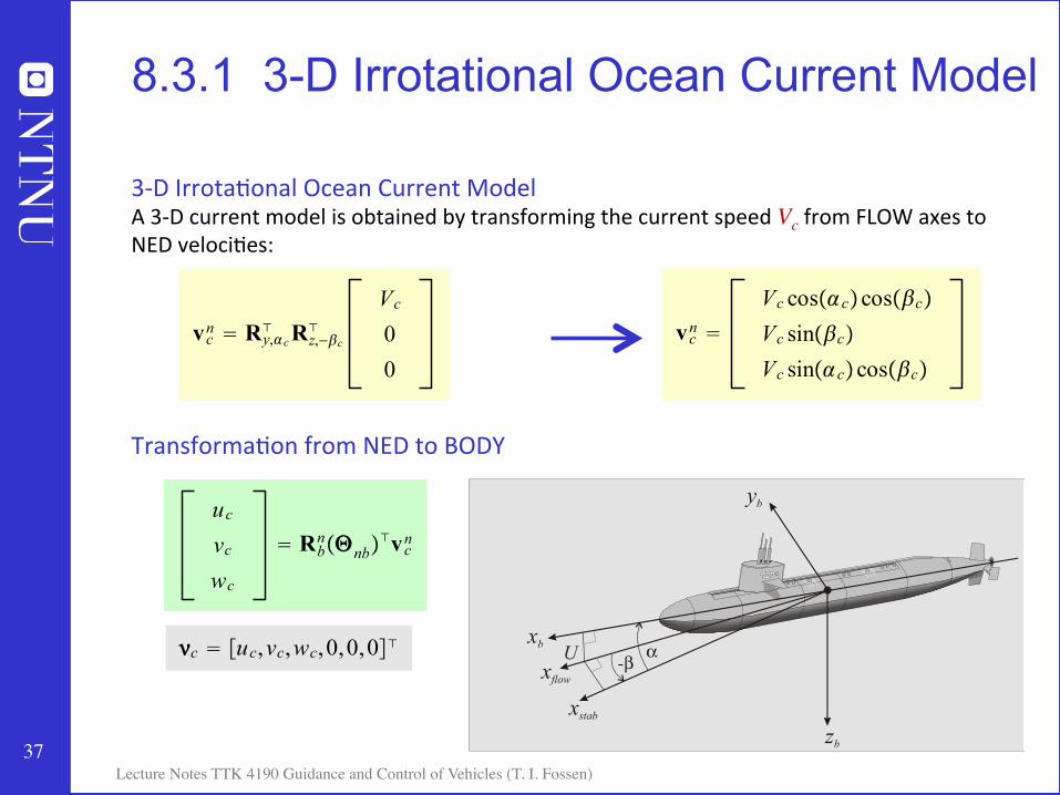
8.3.1 3-D Irrotational Ocean Current Model
3-‐D Irrota;onal Ocean Current Model A 3-‐D current model is obtained by transforming the current speed Vc from FLOW axes to NED veloci;es: Transforma;on from NED to BODY
!c ! !uc,vc,wc,0,0,0"! #
vcn ! Ry,!c! Rz,!"c!
Vc00
# vcn !Vc cos!!c"cos!"c"Vc sin!"c"Vc sin!!c"cos!"c"
#
ucvcwc
! Rbn!!nb"!vcn #
xb α-β
xstabzb
yb
Uxflow

38 Lecture Notes TTK 4190 Guidance and Control of Vehicles (T. I. Fossen)
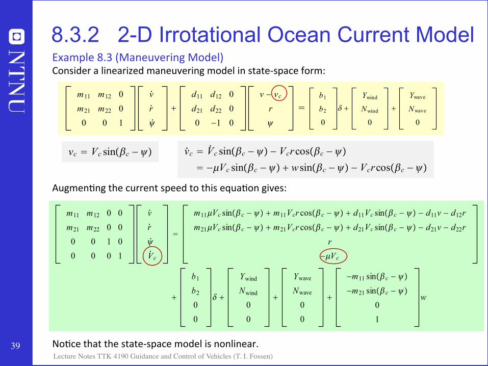
8.3.2 2-D Irrotational Ocean Current Model
2-‐D Ocean Current Model For the 2-‐D case, the 3-‐D equa;ons with αc = 0 reduces to: These expressions are used to compute current forces for ships using:
• Current coefficients • Cross-‐flow drag
For underwater vehicles the 3-‐D representa;on should be used.
uc ! Vc cos!!c ! ""
vc ! Vc sin!!c ! ""
# #
vcn !Vc cos!!c"Vc sin!!c"
0 #
Vc ! uc2 " vc2 #
39 Lecture Notes TTK 4190 Guidance and Control of Vehicles (T. I. Fossen)
m11 m12 0 0m21 m22 0 00 0 1 00 0 0 1
v!r!!!
V! c
"
m11"Vc sin!# c ! !" # m11Vcr cos!# c ! !" # d11Vc sin!# c ! !" ! d11v ! d12rm21"Vc sin!# c ! !" # m21Vcr cos!# c ! !" # d21Vc sin!# c ! !" ! d21v ! d22r
r!"Vc
#
b1b200
$ #
YwindNwind00
#
YwaveNwave00
#
!m11 sin!# c ! !"
!m21 sin!# c ! !"
01
w #
Example 8.3 (Maneuvering Model) Consider a linearized maneuvering model in state-‐space form: Augmen;ng the current speed to this equa;on gives: No;ce that the state-‐space model is nonlinear.
8.3.2 2-D Irrotational Ocean Current Model
m11 m12 0m21 m22 00 0 1
v!r!!!
"
d11 d12 0d21 d22 00 !1 0
v ! vc
r!
#b1b20
" "
YwindNwind
0
"
YwaveNwave
0
#
vc ! Vc sin!!c ! "" # v! c " V! c sin!!c ! "" ! Vcrcos!!c ! ""
" !#Vc sin!!c ! "" # wsin!!c ! "" ! Vcrcos!!c ! ""
# #