Embed Size (px)
Citation preview
Introduction to Communications Prof. Jae Hong Lee, SNU Chapter 8. Digital Transmission through Bandlimited AWGN Channels - 1 - 1st Semester, 2008
Chpater 8 Digital Transmission through Bandlimited AWGN Channels
Text. [1] J. G. Proakis and M. Salehi, Communication Systems Engineering, 2/e. Prentice Hall, 2002.
8.1 Digital Transmission through Bandlimited Channels
8.2 Power Spectral Density of the Baseband Signal
8.3 Signal Design for Bandlimited Channels
8.4 Probability of Error in Detection of Digital PAM
8.5 Digitally Modulated Signals with Memory (partly skipped)
8.6 System Design in the Presence of Channel Distortion (skipped)
8.7 Multicarrier Modulation and OFDM (briefly covered)
Digital communication over a channel is modeled as a linear filter with a bandwidth limitation.
Bandlimited channels most frequently are encountered in telephone channels, microwave LOS radio
channels, satellite channels, and underwater acoustic channels.
Introduction to Communications Prof. Jae Hong Lee, SNU Chapter 8. Digital Transmission through Bandlimited AWGN Channels - 2 - 1st Semester, 2008
The transmitted signals must be designed to satisfy the bandwidth constraint imposed by the channel, that is,
the transmitted signals must be shaped to restrict their bandwidth to that available on the channel.
8.1 Digital Transmission through Bandlimited Channels
A bandlimited channel is characterized as a linear filter with impulse response ( )c t and frequency response
( )C f which is given by
2( ) ( ) j f tC f c t e dtπ∞ −
−∞= ∫ . (8.1.1)
If the channel is a baseband channel that is bandlimited to cB Hz, then
( ) 0C f = for | | cf B> .
Any frequency components with frequency higher than cB Hz will not be passed by the channel which is
bandlimited to cW B= Hz as shown in Figure 8.1.

Introduction to Communications Prof. Jae Hong Lee, SNU Chapter 8. Digital Transmission through Bandlimited AWGN Channels - 3 - 1st Semester, 2008
Introduction to Communications Prof. Jae Hong Lee, SNU Chapter 8. Digital Transmission through Bandlimited AWGN Channels - 4 - 1st Semester, 2008
Let W denote the bandwidth limitation of the signal and the channel.
Suppose that the input to a bandlimited channel is a signal ( )Tg t .
Then, the output of the channel corresponding to the input ( )Tg t is given by
( ) ( ) ( )Th t c g t dτ τ τ∞
−∞= −∫
( ) ( )Tc t g t= ∗ (8.1.2)
or, in the frequency domain, we have
( ) ( ) ( )TH f C f G f= (8.1.3)
where ( )TG f is the spectrum (Fourier transform) of the signal ( )Tg t and ( )H f is the spectrum of ( )h t .
Assume that the signal at the input to the demodulator (that is, at the output of the channel) is corrupted by
AWGN which is given by ( ) ( )h t n t+ where ( )n t is the AWGN.
In the presence of AWGN, a demodulator having a filter which is matched to the signal ( )h t maximizes
Introduction to Communications Prof. Jae Hong Lee, SNU Chapter 8. Digital Transmission through Bandlimited AWGN Channels - 5 - 1st Semester, 2008
the SNR at its output.
Let the received signal ( ) ( )h t n t+ is passed through the matched filter of which frequency response is
given by
02( ) ( ) j f tRG f H f e π−∗= (8.1.4)
where 0t is time delay at which the filter output is sampled.
The signal component at the output of the matched filter at the sampling instant 0t t= is given by
20( ) | ( ) |Sy t H f df
∞
−∞= ∫
hε= (8.1.5)
which is the energy in the channel output ( )h t .
The noise component at the output of the matched filter has zero mean and a power-spectral density given
by
20( ) | ( ) |2nNS f H f= . (8.1.6)
Introduction to Communications Prof. Jae Hong Lee, SNU Chapter 8. Digital Transmission through Bandlimited AWGN Channels - 6 - 1st Semester, 2008
Hence, the noise power at the output of the matched filter has a variance
2 ( )n nS f dfσ∞
−∞= ∫
20 | ( ) |2N H f df
∞
−∞= ∫
0
2hN ε
= (8.1.7)
The SNR at the output of the matched filter is given by 2
00
2
h
h
SNNεε
⎛ ⎞ =⎜ ⎟⎝ ⎠
0
2 h
Nε
= (8.1.8)
which is the same as SNR at the output of the matched filter in Chapter 7 except that the received signal nergy
hε has replaced the transmitted signal energy Sε .
Note that the filter impulse response is matched to the signal component ( )h t in the received signal instead
of the transmitted signal.
Introduction to Communications Prof. Jae Hong Lee, SNU Chapter 8. Digital Transmission through Bandlimited AWGN Channels - 7 - 1st Semester, 2008
Note that to implement the matched filter at the receiver, ( )h t (or, equivalently, the channel impulse
response ( )c t ) must be known to the receiver.
Ex. 8.1.1
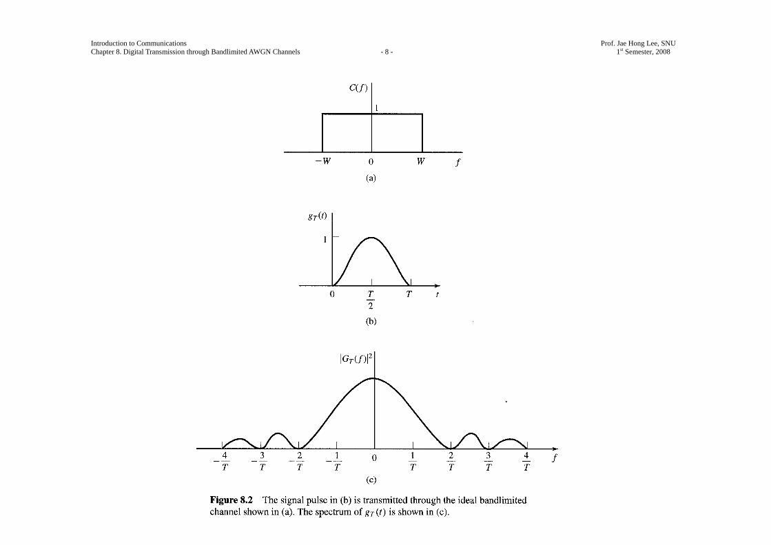
The signal ( )Tg t is given by
1 2( ) 1 cos2 2T
Tg t tTπ⎡ ⎤⎛ ⎞= + −⎜ ⎟⎢ ⎥⎝ ⎠⎣ ⎦
, 0 t T≤ ≤ ,
which is shown in Figure 8.2(b).
( )Tg t is transmitted through a baseband channel with frequency-response characteristic as shown in Figure
8.2(a).
Introduction to Communications Prof. Jae Hong Lee, SNU Chapter 8. Digital Transmission through Bandlimited AWGN Channels - 8 - 1st Semester, 2008
Introduction to Communications Prof. Jae Hong Lee, SNU Chapter 8. Digital Transmission through Bandlimited AWGN Channels - 9 - 1st Semester, 2008
The channel output is corrupted by AWGN with power-spectral density 0
2N .
Determine the matched filter to the received signal and the output SNR.
Solution
The spectrum of the signal is given by
2 2
sin( )2 (1 )
j f TT
T fTG f efT f T
πππ
−=−
2 2
sinc2 (1 )
j f TT fT ef T
ππ −=−
of which square, 2| ( ) |TG f , is shown in Figure 8.2(c).
Hence,
( ) ( ) ( )TH f C f G f=
( ), | | ,0, otherwise.
TG f f W≤⎧= ⎨⎩
Introduction to Communications Prof. Jae Hong Lee, SNU Chapter 8. Digital Transmission through Bandlimited AWGN Channels - 10 - 1st Semester, 2008
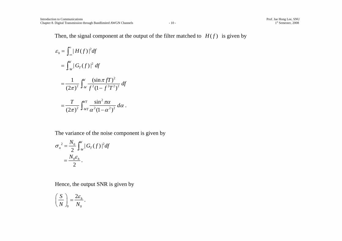
Then, the signal component at the output of the filter matched to ( )H f is given by
2| ( ) |h H f dfε∞
−∞= ∫
2| ( ) |W
TWG f df
−= ∫
2
2 2 2 2 2
1 (sin )(2 ) (1 )
W
W
fT dff f T
ππ −
=−∫
2
2 2 2 2
sin(2 ) (1 )
WT
WT
T dπα απ α α−
=−∫ .
The variance of the noise component is given by
2 20 | ( ) |2
W
n TW
N G f dfσ−
= ∫
0
2hN ε
= .
Hence, the output SNR is given by
0 0
2 hSN N
ε⎛ ⎞ =⎜ ⎟⎝ ⎠
.
Introduction to Communications Prof. Jae Hong Lee, SNU Chapter 8. Digital Transmission through Bandlimited AWGN Channels - 11 - 1st Semester, 2008
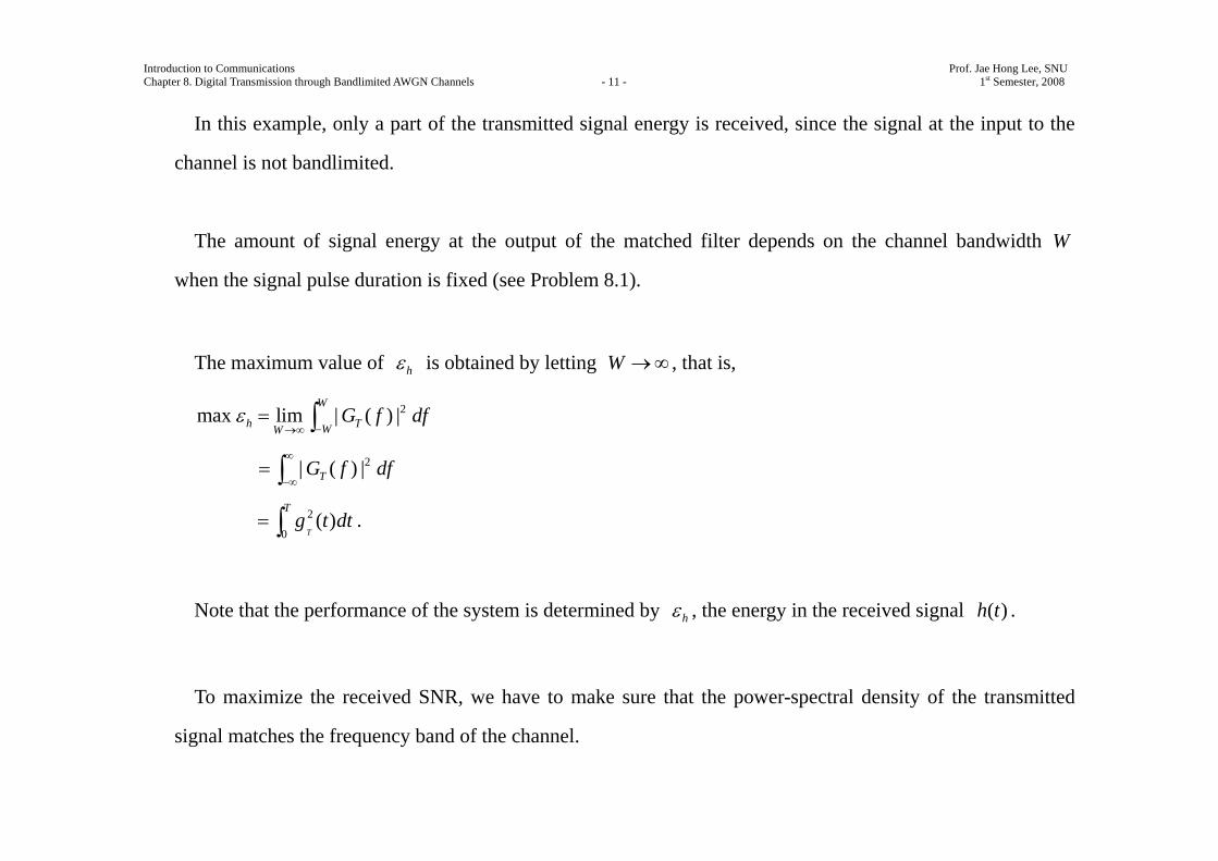
In this example, only a part of the transmitted signal energy is received, since the signal at the input to the
channel is not bandlimited.
The amount of signal energy at the output of the matched filter depends on the channel bandwidth W
when the signal pulse duration is fixed (see Problem 8.1).
The maximum value of hε is obtained by letting W →∞ , that is,
2max lim | ( ) |W
h TWWG f dfε
−→∞= ∫
2| ( ) |TG f df∞
−∞= ∫
2
0( )
T
Tg t dt= ∫ .
Note that the performance of the system is determined by hε , the energy in the received signal ( )h t .
To maximize the received SNR, we have to make sure that the power-spectral density of the transmitted
signal matches the frequency band of the channel.
Introduction to Communications Prof. Jae Hong Lee, SNU Chapter 8. Digital Transmission through Bandlimited AWGN Channels - 12 - 1st Semester, 2008
8.1.1 Digital PAM Transmission through Bandlimited Baseband Channels
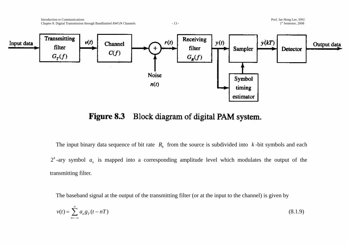
Consider the baseband PAM communication system shown by the block diagram in Figure 8.3.
The system consists of a transmitting filter having an impulse response ( )Tg t , the linear filter channel with
AWGN, a receiving filter with impulse response ( )Rg t , a sampler that periodically samples the output of
receiving filter, and a symbol detector.
The sampler needs a timing signal whch is extracted from the received signal (see Section 7.8) to serve as a
clock to specify the appropriate time instants to sample the output of the receiving filter.
Introduction to Communications Prof. Jae Hong Lee, SNU Chapter 8. Digital Transmission through Bandlimited AWGN Channels - 13 - 1st Semester, 2008
The input binary data sequence of bit rate bR from the source is subdivided into k -bit symbols and each
2k -ary symbol na is mapped into a corresponding amplitude level which modulates the output of the
transmitting filter.
The baseband signal at the output of the transmitting filter (or at the input to the channel) is given by
( ) ( )n Tn
v t a g t nT∞
=−∞
= −∑ (8.1.9)
Introduction to Communications Prof. Jae Hong Lee, SNU Chapter 8. Digital Transmission through Bandlimited AWGN Channels - 14 - 1st Semester, 2008
where b
kTR
= is the symbol interval.
Note that the symbol rate is given by 1 bRT k= .
The received signal at the demodulator (or the channel output) is given by
( ) ( ) ( )nn
r t a h t nT n t∞
=−∞
= − +∑ (8.1.10)
where ( )h t is the impulse response of the cascade of the transmitting filter and the channel, that is,
( ) ( ) ( )Th t c t g t= ∗ ,
( )c t is the impulse response of the channel, and
( )n t is an AWGN.
The received signal is passed through a linear receiving filter with impulse response ( )Rg t and frequency
response ( )RG f .
Introduction to Communications Prof. Jae Hong Lee, SNU Chapter 8. Digital Transmission through Bandlimited AWGN Channels - 15 - 1st Semester, 2008
If ( )Rg t is matched to ( )h t , then its output SNR becomes a maximum at the proper sampling instant.
The output of the receiving filter is given by
( ) ( ) ( )nn
y t a x t nT v t∞
=−∞
= − +∑ (8.1.11)
where ( ) ( ) ( ) ( ) ( ) ( )R T Rx t h t g t g t c t g t= ∗ = ∗ ∗ and
( ) ( ) ( )Rv t n t g t= ∗ is the additive noise at the output of the receiving filter.
To recover the information symbols { }na , the output of the receiving filter is sample periodically with the
interval of T seconds.
The output of the sampler is given by
( ) ( ) ( )nn
y mT a x mT nT v mT∞
=−∞
= − +∑ (8.1.12)
or, equivalently,
Introduction to Communications Prof. Jae Hong Lee, SNU Chapter 8. Digital Transmission through Bandlimited AWGN Channels - 16 - 1st Semester, 2008
m n m n mn
y a x v∞
−=−∞
= +∑
0 m n m n mnn m
x a a x v∞
−=−∞≠
= + +∑ (8.1.13)
where ( )mx x mT= and
( )mv v mT= for , 2, 1, 0,1, 2, .m = − −
The first term, 0 mx a , on the right-hand side (RHS) of (8.1.13) is the desired symbol ma scaled by the gain
parameter 0x .
When the receiving filter is matched to the received signal ( )h t , the scale factor is given by
20 ( )x h t dt
∞
−∞= ∫
2| ( ) |H f df∞
−∞= ∫
2 2| ( ) | | ( ) |W
TWG f C f df
−= ∫
hε= (8.1.14)
Introduction to Communications Prof. Jae Hong Lee, SNU Chapter 8. Digital Transmission through Bandlimited AWGN Channels - 17 - 1st Semester, 2008
as shown in (8.1.4) and (8.1.5).
The second term on the RHS of (8.1.13) represents the intersymbol interference (ISI) which is the effect
of the other symbols to the desired symbols at the sampling instant t mT= .
In general, ISI degrades the performance of the digital communication system.
The third term, mv , on the RHS of (8.1.13) is the additive noise and is a zero-mean Gaussian random
variable with variance 2 0
2h
vN εσ = as given by (8.1.7).
By appropriate design of the transmitting and receiving filters, it is possible to satisfy the condition 0nx =
for all 0n ≠ , so that the ISI term vanishes.
In this case, the only term which causes errors in the received digital sequence is the additive noise.
Introduction to Communications Prof. Jae Hong Lee, SNU Chapter 8. Digital Transmission through Bandlimited AWGN Channels - 18 - 1st Semester, 2008
8.1.2 Digital Transmission through Bandlimited Bandpass Channels
The development given in Section 8.1.1 for baseband PAM is easily extended to carrier modulation via PAM,
and QAM and PSK.
In a carrier-amplitude modulated signal (or bandpass PAM or ASK), the baseband PAM given by ( )v t in
(8.1.9) modulates the carrier, so that the transmitted signal is given by
( ) ( )cos2 ,cu t v t f tπ= (8.1.15)
which implies that the baseband signal ( )v t is shifted in frequency by cf .
A QAM signal is a bandpass signal.
A rectangular QAM signal may be viewed as two amplitude-modulated carrier signals in phase quadrature.
That is, the QAM signal is given by
( ) ( )cos2 ( )sin 2c c s cu t v t f t v t f tπ π= + (8.1.16)
Introduction to Communications Prof. Jae Hong Lee, SNU Chapter 8. Digital Transmission through Bandlimited AWGN Channels - 19 - 1st Semester, 2008
where
( ) ( )c n c Tn
v t a g t nT∞
=−∞
= −∑ ,
( ) ( )s n s Tn
v t a g t nT∞
=−∞
= −∑ (8.1.17)
and { }nca and { }nsa are the two sequences of amplitudes carried on the two quadrature carriers.
An equivalent complex-valued baseband signal of the QAM signal is given by
( ) ( ) ( )c sv t v t jv t= −
( ) ( )n c n s Tn
a ja g t nT∞
=−∞
= − −∑
( )n Tn
a g t nT∞
=−∞
= −∑ (8.1.18)
where n n c n sa a ja= − and the sequence { }na is a complex-valued sequence representing the signal points in
the QAM signal constellation.

Introduction to Communications Prof. Jae Hong Lee, SNU Chapter 8. Digital Transmission through Bandlimited AWGN Channels - 20 - 1st Semester, 2008
From (8.1.16) and (8.1.18), the corresponding bandpass QAM signal is given by
2( ) Re ( ) cj f tu t v t e π⎡ ⎤= ⎣ ⎦ . (8.1.19)
Similarly to (8.1.19), an equivalent complex-valued baseband (or PSK) signal is given by
( ) ( )n Tn
v t a g t nT∞
=−∞
= −∑ (8.1.20)
and the sequence { }na takes the value from the set of possible (phase) values 2
{ , 0,1, , 1}mjMe m M
π−= − .
All three carrier-modulated signals for PAM, QAM, and PSK can be represented as in (8.1.19) and (8.1.20),
where the only difference is in the values of the transmitted sequence { }na .
The signal ( )v t given by (8.1.19) or (8.1.20) is called the equivalent lowpass signal.
In the case of QAM and PSK, the equivalent lowpass signal ( )v t is a complex-valued baseband signal
because the information-bearing sequence { }na is complex-valued.
Introduction to Communications Prof. Jae Hong Lee, SNU Chapter 8. Digital Transmission through Bandlimited AWGN Channels - 21 - 1st Semester, 2008
In the case of PAM, the equivalent lowpass signal ( )v t is a real-valued baseband signal.
Suppose that the channel has the impulse response of the equivalent lowpass channel ( )c t .
Then, when transmitted through the bandpass channel, the received bandpass signal is given by
2( ) Re ( ) cj f tw t r t e π⎡ ⎤= ⎣ ⎦ (8.1.21)
where ( )r t is the equivalent lowpass (baseband) signal, which is given by
( ) ( ) ( )nn
r t a h t nT n t∞
=−∞
= − +∑ (8.1.22)
where ( )h t is the impulse response of the cascade of the transmitting filter and the channel, that is,
( ) ( ) ( )Th t c t g t= ∗ , and
( )n t is the additive Gaussian noise expressed as an equivalent lowpass (baseband) noise.
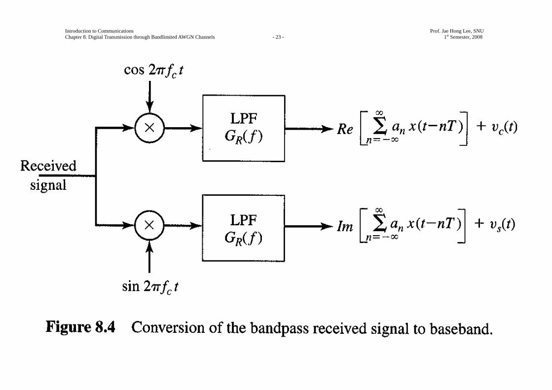
The received bandpass signal can be converted to a baseband signal by multiplying ( )w t with the
Introduction to Communications Prof. Jae Hong Lee, SNU Chapter 8. Digital Transmission through Bandlimited AWGN Channels - 22 - 1st Semester, 2008
quadrature carrier signals cos2 cf tπ and sin 2 cf tπ and eliminating the double frequency terms by passing
the two quadrature components through two separate lowpass filters, as shown in Figure 8.4.
Introduction to Communications Prof. Jae Hong Lee, SNU Chapter 8. Digital Transmission through Bandlimited AWGN Channels - 23 - 1st Semester, 2008
Introduction to Communications Prof. Jae Hong Lee, SNU Chapter 8. Digital Transmission through Bandlimited AWGN Channels - 24 - 1st Semester, 2008
Assume each of the lowpass filters in Figure 8.4 has an impulse response ( )Rg t .
Then, we can represent the two quadrature components at the outputs of the two lowpass filters as an
equivalent complex-valued signal
( ) ( ) ( )nn
y t a x t nT v t∞
=−∞
= − +∑ (8.1.23)
which is identical to (8.1.11) for the real baseband signal.
Hence, the signal design problem for bandpass signals is basically the same as that for baseband signals.
8.2 Power Spectral Density of Digitally Modulated Signals
Introduction to Communications Prof. Jae Hong Lee, SNU Chapter 8. Digital Transmission through Bandlimited AWGN Channels - 25 - 1st Semester, 2008
8.2.1 Power Spectral Density of the Baseband Signal
The equivalent baseband transmitted signal for a digital PAM, PSK, or QAM signal is represented in the
general form as
( ) ( )n Tn
v t a g t nT∞
=−∞
= −∑ (8.2.1)
where { }na is the sequence of values selected from either a PAM, QAM, or PSK signal constellation
corresponding to the information symbols from the source, and
( )Tg t is the impulse response of the transmitting filter.
Since the information sequence { }na is random, ( )v t is a sample function of a random process ( )V t .
The mean function of the random variable (or the baseband transmitted signal) ( )v t is given by
[ ( )] [ ] ( )n Tn
E V t E a g t nT∞
=−∞
= −∑
Introduction to Communications Prof. Jae Hong Lee, SNU Chapter 8. Digital Transmission through Bandlimited AWGN Channels - 26 - 1st Semester, 2008
( )a Tn
m g t nT∞
=−∞
= −∑ (8.2.2)
where am is the mean of the random variable na .
Note that, since although am is a constant, the term ( )tn
g t nT−∑ in (8.2.2) is a periodic function with
period T , the mean function of ( )V t is periodic with period T .
The autocorrelation function of ( )V t is given by
*( , ) [ ( ) ( )]VR t t E V t V tτ τ+ = +
[ ] ( ) ( )n m T Tn m
E a a g t nT g t mTτ∞ ∞
∗
=−∞ =−∞
= − + −∑ ∑ . (8.2.3)
Assume that the information sequence { }na is wide-sense stationary with the autocorrelation function
given by
( ) [ ]a m n mR n E a a∗ += . (8.2.4)
Introduction to Communications Prof. Jae Hong Lee, SNU Chapter 8. Digital Transmission through Bandlimited AWGN Channels - 27 - 1st Semester, 2008
Then, (8.2.3) becomes
( , ) ( ) ( ) ( )V a T Tn m
R t t R m n g t nT g t mTτ τ∞ ∞
=−∞ =−∞
+ = − − + −∑ ∑
( ) ( ) ( )a T Tm n
R m g t nT g t nT mTτ∞ ∞
=−∞ =−∞
= − + − −∑ ∑ . (8.2.5)
where the second summation ( ) ( )T Tn
g t nT g t nT mTτ∞
=−∞
− + − −∑ is periodic with period T .
Consequently, the autocorrelation function ( , )VR t tτ+ is periodic in the variable t , that is,
( , ) ( , )V VR t T t T R t tτ τ+ + + = + . (8.2.7)
Since the random process ( )V t has a periodic mean function and a periodic autocorrelation function, the
random process ( )V t is cyclostationary (see Definition 4.2.7).
Introduction to Communications Prof. Jae Hong Lee, SNU Chapter 8. Digital Transmission through Bandlimited AWGN Channels - 28 - 1st Semester, 2008
The power-spectral density of a cyclostationary process ( )V t is determined by averaging the
autocorrelation function ( , )VR t tτ+ over a period T and then computing the Fourier transform of the
average autocorrelation function (see Corollary to Theorem 4.3.1).
The average autocorrelation function of ( )V t is given by
2
2
1( ) ( , )T
TV VR R t t dtT
τ τ−
= +∫
2
2
1( ) ( ) ( )T
Ta T Tm n
R m g t nT g t nT mT dtT
τ∞ ∞
−=−∞ =−∞
= − + − −∑ ∑ ∫
2
2
1( ) ( ) ( )TnT
Ta T TnTm n
R m g t g t mT dtT
τ∞ ∞ +
−=−∞ =−∞
= + −∑ ∑ ∫
1 ( ) ( ) ( )a T Tm
R m g t g t mT dtT
τ∞ ∞
−∞=−∞
= + −∑ ∫ (8.2.8)
The integral in (8.2.8) is the time-autocorrelation function of ( )Tg t which is defined as (See (2.3.1))
( ) ( ) ( )g T TR g t g t dtτ τ∞
−∞+∫ . (8.2.9)
Introduction to Communications Prof. Jae Hong Lee, SNU Chapter 8. Digital Transmission through Bandlimited AWGN Channels - 29 - 1st Semester, 2008
From (8.2.8) and (8.2.9) it becomes
1( ) ( ) ( )V a gm
R R m R mTT
τ τ∞
=−∞
= −∑ (8.2.10)
which has the form of a convolution sum.
Hence the Fourier transform of the average autocorrelation function of ( )V t in (8.2.10) is given by
2( ) ( ) j fV VS f R e dπ ττ τ
∞ −
−∞= ∫
21 ( ) ( ) j fa g
m
R m R mT e dT
π ττ τ∞ ∞ −
−∞=−∞
= −∑ ∫
21 ( ) | ( ) |a TS f G fT
= (8.2.11)
where ( )aS f is the power spectral density of the information sequence { }na given by
2( ) ( ) f mTa a
m
S f R m e π∞
−
=−∞
= ∑ (8.2.12)
and ( )TG f is the transfer function of the transmitting filter.
2| ( ) |TG f is the Fourier transform of ( )gR τ .
Introduction to Communications Prof. Jae Hong Lee, SNU Chapter 8. Digital Transmission through Bandlimited AWGN Channels - 30 - 1st Semester, 2008
From (8.2.11), notice that the power-spectral density ( )VS f of the transmitted signal ( )V t depends on (1)
the transfer function ( )TG f of the transmitting filter and (2) the power spectral density ( )aS f of the
information sequence { }na .
Both ( )TG f and ( )aS f can be designed to adjuct the shape of the power spectral density of the
transmitted signal.
Examine the dependence of ( )VS f on ( )aS f .
First, we observe that, for an arbitrary autocorrelation function ( )aR m , the corresponding power-spectral
density ( )aS f is periodic in frequency with period 1T
.
Note that ( )aS f in (8.2.12) is an exponential Fourier series with the Fourier coefficients { ( )}aR m .
Introduction to Communications Prof. Jae Hong Lee, SNU Chapter 8. Digital Transmission through Bandlimited AWGN Channels - 31 - 1st Semester, 2008
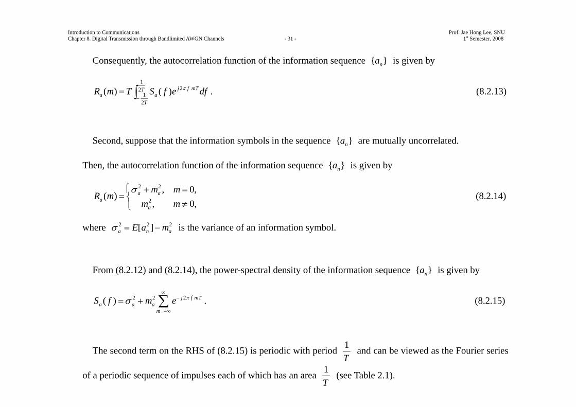
Consequently, the autocorrelation function of the information sequence { }na is given by
122
12
( ) ( ) j f mTTa a
T
R m T S f e dfπ
−= ∫ . (8.2.13)
Second, suppose that the information symbols in the sequence { }na are mutually uncorrelated.
Then, the autocorrelation function of the information sequence { }na is given by
2 2
2
, 0,( )
, 0,a a
aa
m mR m
m mσ⎧ + =
= ⎨≠⎩
(8.2.14)
where 2 2 2[ ]a n aE a mσ = − is the variance of an information symbol.
From (8.2.12) and (8.2.14), the power-spectral density of the information sequence { }na is given by
2 2 2( ) j f mTa a a
m
S f m e πσ∞
−
=−∞
= + ∑ . (8.2.15)
The second term on the RHS of (8.2.15) is periodic with period 1T
and can be viewed as the Fourier series
of a periodic sequence of impulses each of which has an area 1T
(see Table 2.1).

Introduction to Communications Prof. Jae Hong Lee, SNU Chapter 8. Digital Transmission through Bandlimited AWGN Channels - 32 - 1st Semester, 2008
Therefore, (8.2.15) is expressed as
2 2 1( ) ( )a a am
mS f m fT T
σ δ∞
=−∞
= + −∑ . (8.2.16)
From (8.2.11) and (8.2.16), the power-spectral density of the transmitted signal ( )V t , when the sequence of
information symbols is uncorrelated, is given by
2 22 2
2( ) | ( ) | | |a aV T T
m
m m mS f G f G fT T T Tσ δ
∞
=−∞
⎛ ⎞ ⎛ ⎞= + −⎜ ⎟ ⎜ ⎟⎝ ⎠ ⎝ ⎠
∑ . (8.2.17)
The first term on the RHS of (8.2.17), 2
2| ( ) |aTG f
Tσ , is a continuous dunction and its shape depends of
( )TG f .
The second term in (8.2.17) consists of discrete frequency components spaced 1T
apart in frequency.
Each component (or spectral line) has power that is proportional to 2| ( ) |TG f at mfT
= .
Introduction to Communications Prof. Jae Hong Lee, SNU Chapter 8. Digital Transmission through Bandlimited AWGN Channels - 33 - 1st Semester, 2008
Note that the discrete frequency components can be eliminated by selecting the information symbol
sequence { }na to have zero mean.
The mean am in digital PAM, PSK, or QAM signals is easily forced to be zero by selecting the signal
constellation points to be symmetrically positioned in the complex plane relative to the origin.
Under the condition that 0am = , the power-spectral density of the transmitted signal ( )V t becomes
22( ) | ( ) |a
V TS f G fTσ
= . (8.2.18)
Thus, the system designer can control the spectral characteristics of the transmitted digital PAM signal.
Ex. 8.2.1
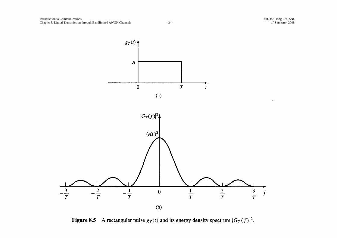
Determine the power-spectral density of the transmitted signal ( )V t in (8.2.17), when ( )Tg t is the
rectangular pulse shown in Figure 8.5(a).
Introduction to Communications Prof. Jae Hong Lee, SNU Chapter 8. Digital Transmission through Bandlimited AWGN Channels - 34 - 1st Semester, 2008
Introduction to Communications Prof. Jae Hong Lee, SNU Chapter 8. Digital Transmission through Bandlimited AWGN Channels - 35 - 1st Semester, 2008
Solution
The Fourier transform of ( )Tg t is given by
sin( ) j f TT
fTG f AT efT
πππ
−= .
Hence, 2
2 2 sin| ( ) | ( )TfTG f AT
fTπ
π⎛ ⎞
= ⎜ ⎟⎝ ⎠
2 2( ) sinc ( )AT fT=
which is shown in Figure 8.5(b).
Note that it contains nulls at multiples of 1T
in frequency and that it decays inversely as the square of the
frequency variable.
As a consequence of the spectral nulls in ( )TG f , all but one of the discrete spectral components in (8.2.17)
vanish.
Introduction to Communications Prof. Jae Hong Lee, SNU Chapter 8. Digital Transmission through Bandlimited AWGN Channels - 36 - 1st Semester, 2008
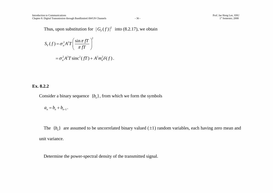
Thus, upon substitution for 2| ( ) |TG f into (8.2.17), we obtain
22 2 sin( )V a
fTS f A TfTπσ
π⎛ ⎞
= ⎜ ⎟⎝ ⎠
2 2 2 2 2sinc ( ) ( )a aA T fT A m fσ δ= + .
Ex. 8.2.2
Consider a binary sequence { }nb , from which we form the symbols
1n n na b b −= + .
The { }nb are assumed to be uncorrelated binary valued ( 1± ) random variables, each having zero mean and
unit variance.
Determine the power-spectral density of the transmitted signal.
Introduction to Communications Prof. Jae Hong Lee, SNU Chapter 8. Digital Transmission through Bandlimited AWGN Channels - 37 - 1st Semester, 2008
Solution
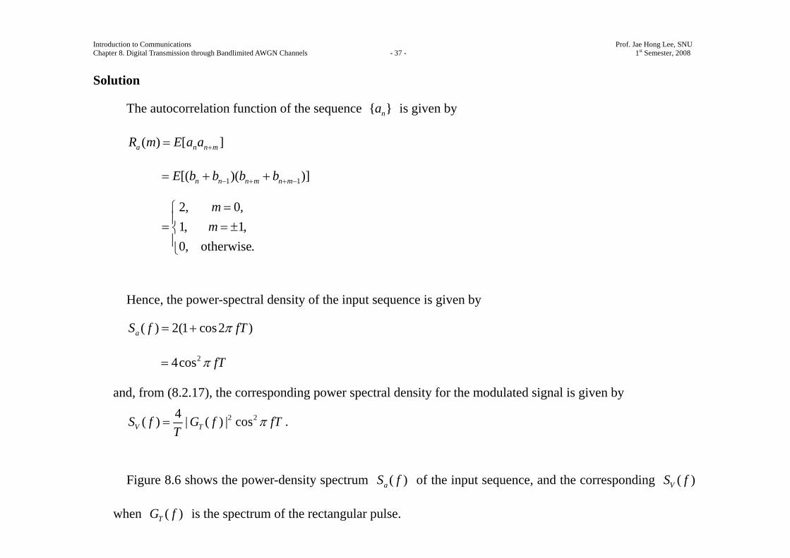
The autocorrelation function of the sequence { }na is given by
( ) [ ]a n n mR m E a a +=
1 1[( )( )]n n n m n mE b b b b− + + −= + +
2, 0,1, 1,0, otherwise.
mm
=⎧⎪= = ±⎨⎪⎩
Hence, the power-spectral density of the input sequence is given by
( ) 2(1 cos2 )aS f fTπ= +
24cos fTπ=
and, from (8.2.17), the corresponding power spectral density for the modulated signal is given by
2 24( ) | ( ) | cosV TS f G f fTT
π= .
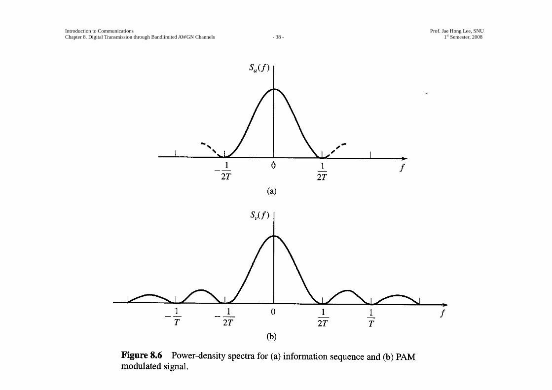
Figure 8.6 shows the power-density spectrum ( )aS f of the input sequence, and the corresponding ( )VS f
when ( )TG f is the spectrum of the rectangular pulse.
Introduction to Communications Prof. Jae Hong Lee, SNU Chapter 8. Digital Transmission through Bandlimited AWGN Channels - 38 - 1st Semester, 2008
Introduction to Communications Prof. Jae Hong Lee, SNU Chapter 8. Digital Transmission through Bandlimited AWGN Channels - 39 - 1st Semester, 2008
As demonstrated in the example, the power spectral density of the transmitted signal can be shaped by
having a correlated sequence { }na as the input to the modulator.
8.2.2 Power Spectral Density of a Carrier-Modulated Signal
The autocorrelation function of the information sequence { }na is given by
*( ) [ ]a n n mR m E a a += . (8.2.21)
The power spectral density of the information sequence { }na is given by
2( ) ( ) j fmTa a
m
S f R m e π∞
−
=−∞
= ∑ . (8.2.20)
In Section 8.2.1, it was shown that the power spectral density of the equivalent baseband signal ( )v t in
(8.2.1) for bandpass PAM, QAM, and PSK is given by
Introduction to Communications Prof. Jae Hong Lee, SNU Chapter 8. Digital Transmission through Bandlimited AWGN Channels - 40 - 1st Semester, 2008
21( ) ( ) | ( ) |2V a TS f S f G f= . (8.2.19)
To find out the relationship between the power spectral density of the baseband signal to the power spectral
density of the bandpass signal, consider the bandpass PAM signal as an example.
The autocorrelation function of the bandpass signal
( ) ( )cos2 cu t v t f tπ=
is given by
( , ) [ ( ) ( )]UR t t E U t U tτ τ+ = +
[ ( )]cos2 ( ) cos2c cE VV t f t f tπ τ π= + ⋅
( , )cos2 ( ) cos2V c cR t t f t f tτ π τ π= + + ⋅
1 ( , )[cos2 cos2 (2 )]2 V c cR t t f f tτ π τ π τ= + + + .
Then, the average of ( , )UR t tτ+ over a single period T is given by
1( ) ( )cos22
U V cR R fτ τ π τ= , (8.2.22)
Introduction to Communications Prof. Jae Hong Lee, SNU Chapter 8. Digital Transmission through Bandlimited AWGN Channels - 41 - 1st Semester, 2008
as the second term in the previous equation involving the double frequency averages to zero for each period of
cos4 cf tπ .
The power spectral density of the bandpass signal ( )u t is given by
2( ) ( ) j fU US f R e dπ ττ τ
∞ −
−∞= ∫
1 [ ( ) ( )]4 V c V cS f f S f f= − + + . (8.2.23)
Although (8.2.23) was derived for PAM, it also applies to QAM and PSK.
The bandpass PAM, QAM, and PSK signals differ only in the autocorrelation function ( )aR m of the
sequence { }na and, hence, in the power spectral density ( )aS f of { }na .
Introduction to Communications Prof. Jae Hong Lee, SNU Chapter 8. Digital Transmission through Bandlimited AWGN Channels - 42 - 1st Semester, 2008
8.3 Signal Design for Bandlimited Channels
Consider the problem of designing a bandlimited transmitting filter under thae condition that there is no
channel distortion.
Since ( ) ( ) ( )TH f C f G f= , for distortion-free transmission the frequency response characteristic of the
channel has a constant magnitude and a linear phase over the bandwidth of the transmitted signal, that is,
020 , | | ,
( )0, | | ,
j f tC e f WC f
f W
π−⎧ ≤= ⎨
>⎩ (8.3.3)
where W is the available channel bandwidth,
0t represents an arbitrary finite delay, which we set to zero for convenience, and
0C is a constant gain factor which we set to unity for convenience.
Thus, the distortion-free channel, ( ) ( )TH f G f= for | |f W≤ and zero for | |f W> .
Consequently, the matched filter has a frequency response * *( ) ( )TH f G f= and its output at the periodic
Introduction to Communications Prof. Jae Hong Lee, SNU Chapter 8. Digital Transmission through Bandlimited AWGN Channels - 43 - 1st Semester, 2008
sampling times t mT= has the form
( ) (0) ( ) ( )m nnn m
y mT x a a x mT nT v mT∞
=−∞≠
= + − +∑ (8.3.4)
or, simply
0m m n m n mnn m
y x a a x v∞
−=−∞≠
= + +∑ (8.3.5)
where ( ) ( ) ( )T Rx t g t g t= ∗ and
( )v t is the output response of the matched filter to the input AWGN process ( )n t .
The second term on the RHS of (8.3.5) represents the ISI.
The amount of ISI and noise in the received signal can be viewed on the vertical input of an oscilloscope.
The received signal is displayed on the vertical input with the horizontal sweep rate set at 1T
,.
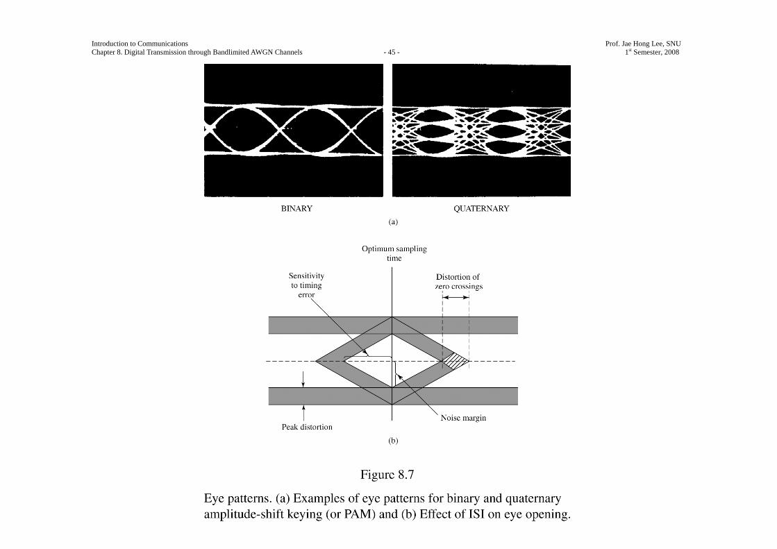
The resulting oscilloscope display is called an eye pattern because of its resemblance to the human eye.
Introduction to Communications Prof. Jae Hong Lee, SNU Chapter 8. Digital Transmission through Bandlimited AWGN Channels - 44 - 1st Semester, 2008
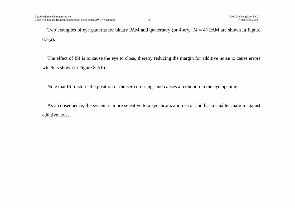
Two examples of eye patterns for binary PAM and quaternary (or 4-ary, 4M = ) PAM are shown in Figure
8.7(a).
The effect of ISI is to cause the eye to close, thereby reducing the margin for additive noise to cause errors
which is shown in Figure 8.7(b).
Note that ISI distorts the position of the zero crossings and causes a reduction in the eye opening.
As a consequence, the system is more sensitive to a synchronization error and has a smaller margin against
additive noise.
Introduction to Communications Prof. Jae Hong Lee, SNU Chapter 8. Digital Transmission through Bandlimited AWGN Channels - 45 - 1st Semester, 2008
Introduction to Communications Prof. Jae Hong Lee, SNU Chapter 8. Digital Transmission through Bandlimited AWGN Channels - 46 - 1st Semester, 2008
8.3.1 Design of Bandlimited Signals for Zero ISI-The Nyquist Criterion
In a digital communication system over a bandlimited channel, the Fourier transform of the signal at the output
of the receiving filter is given by
( ) ( ) ( ) ( )T RX f G f C f G f=
where ( )TG f and ( )RG f denote the transmitter and receiver filters frequency response, respectively, and
( )C f denotes the frequency response of the channel.
We have also seen that the output of the receiving filter, sampled at t mT= , is given by
(0) ( ) ( )m m nnn m
y x a x mT nT a v mT∞
=−∞≠
= + − +∑ . (8.3.6)
To remove the effect of ISI, it is necessary and sufficient that ( ) 0x mT nT− = for n m≠ and (0) 0x ≠ ,
where we can assume (0) 1x = , without loss of generality.†
† The choice of (0)x is equivalent to the choice of a constant gain factor in the receiving filter. This constant gain factor has no effect on the overall system performance since it scales both the signal and the noise.
Introduction to Communications Prof. Jae Hong Lee, SNU Chapter 8. Digital Transmission through Bandlimited AWGN Channels - 47 - 1st Semester, 2008
This implies that the overall communication system has to be designed such that
1, 0,( )
0, 0.n
x nTn=⎧
= ⎨ ≠⎩ (8.3.7)
In this section, we derive the necessary and sufficient condition for ( )X f in order for ( )x t to satisfy the
above relation which is known as the Nyquist pulse-shaping criterion or Nyquist condition for zero ISI.
Theorem 8.3.1 [Nyquist]
A necessary and sufficient condition for ( )x t to satisfy
1, 0,( )
0, 0,n
x nTn=⎧
= ⎨ ≠⎩ (8.3.8)
is that its Fourier transform ( )X f satisfy
m
mX f TT
∞
=−∞
⎛ ⎞+ =⎜ ⎟⎝ ⎠
∑ . (8.3.9)
Proof
In general, ( )x t is the inverse Fourier transform of ( )X f .
Introduction to Communications Prof. Jae Hong Lee, SNU Chapter 8. Digital Transmission through Bandlimited AWGN Channels - 48 - 1st Semester, 2008
Hence,
2( ) ( ) j f tx t X f e dfπ∞
−∞= ∫ . (8.3.10)
At the sampling instants t nT= , this relation becomes
2( ) ( ) j f nTx nT X f e dfπ∞
−∞= ∫ . (8.3.11)
Break up the integral in (8.3.11) into integrals covering the finite range of 1T
.
Then, we obtain
2 122
2 12
( ) ( )m
j f nTTm
m T
x nT X f e dfπ+∞
−=−∞
= ∑ ∫
122
12
j f nTT
m T
mX f e dtT
π∞
−=−∞
⎛ ⎞= +⎜ ⎟⎝ ⎠
∑ ∫
122
12
j f nTT
mT
mX f e dtT
π∞
−=−∞
⎡ ⎤⎛ ⎞= +⎜ ⎟⎢ ⎥⎝ ⎠⎣ ⎦∑∫
122
12
( ) j f nTT
T
Z f e dtπ
−= ∫ (8.3.12)
Introduction to Communications Prof. Jae Hong Lee, SNU Chapter 8. Digital Transmission through Bandlimited AWGN Channels - 49 - 1st Semester, 2008
where
( )m
mZ f X fT
∞
=−∞
⎛ ⎞= +⎜ ⎟⎝ ⎠
∑ . (8.3.13)
As ( )Z f is a periodic function with period 1T
, it can be expanded in terms of its Fourier series
coefficients { }nz as
2( ) j nfTn
m
Z f z e π∞
=−∞
= ∑ (8.3.14)
where
122
12
( ) j nfTTn
T
z T Z f e dfπ−
−= ∫ . (8.3.15)
Comparing (8.3.15) and (8.3.12) we obtain
( )nz T x nT= − . (8.3.16)
Introduction to Communications Prof. Jae Hong Lee, SNU Chapter 8. Digital Transmission through Bandlimited AWGN Channels - 50 - 1st Semester, 2008
Therefore, the necessary and sufficient conditions for (8.3.8) to be satisfied is that
, 0,0, 0,n
T nz
n=⎧
= ⎨ ≠⎩ (8.3.17)
which, when substituted into (8.3.14), yields
( )Z f T= (8.3.18)
or, equivalently,
m
mX f TT
∞
=−∞
⎛ ⎞+ =⎜ ⎟⎝ ⎠
∑ (8.3.19)
which concludes the proof of the theorem.
Now, suppose that the channel has a bandwidth of W .
Then, ( ) 0C f ≡ for | |f W> and consequently, ( ) 0X f = for | |f W> . ( ( ) ( ) ( ) ( )T RX f G f C f G f= )
We distinguish three cases:
Introduction to Communications Prof. Jae Hong Lee, SNU Chapter 8. Digital Transmission through Bandlimited AWGN Channels - 51 - 1st Semester, 2008
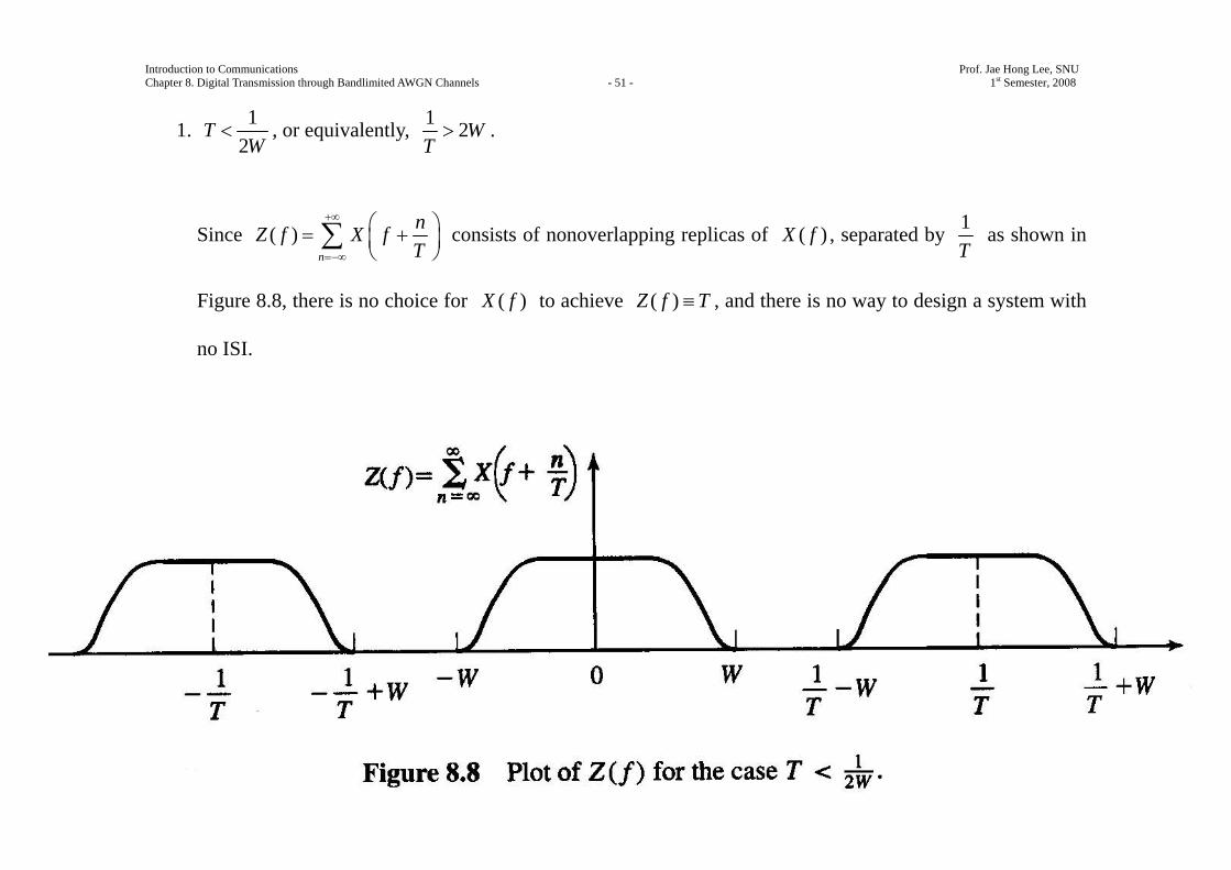
1. 12
TW
< , or equivalently, 1 2WT> .
Since ( )n
nZ f X fT
+∞
=−∞
⎛ ⎞= +⎜ ⎟⎝ ⎠
∑ consists of nonoverlapping replicas of ( )X f , separated by 1T
as shown in
Figure 8.8, there is no choice for ( )X f to achieve ( )Z f T≡ , and there is no way to design a system with
no ISI.
Introduction to Communications Prof. Jae Hong Lee, SNU Chapter 8. Digital Transmission through Bandlimited AWGN Channels - 52 - 1st Semester, 2008
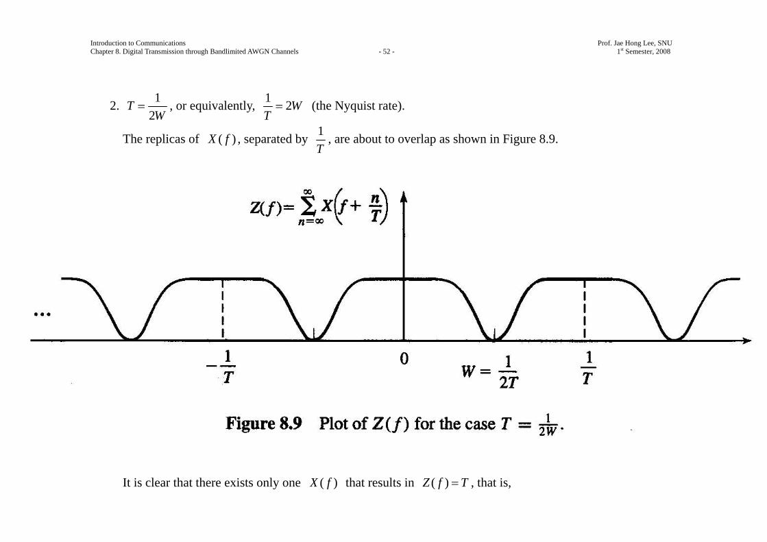
2. 12
TW
= , or equivalently, 1 2WT= (the Nyquist rate).
The replicas of ( )X f , separated by 1T
, are about to overlap as shown in Figure 8.9.
It is clear that there exists only one ( )X f that results in ( )Z f T= , that is,
Introduction to Communications Prof. Jae Hong Lee, SNU Chapter 8. Digital Transmission through Bandlimited AWGN Channels - 53 - 1st Semester, 2008
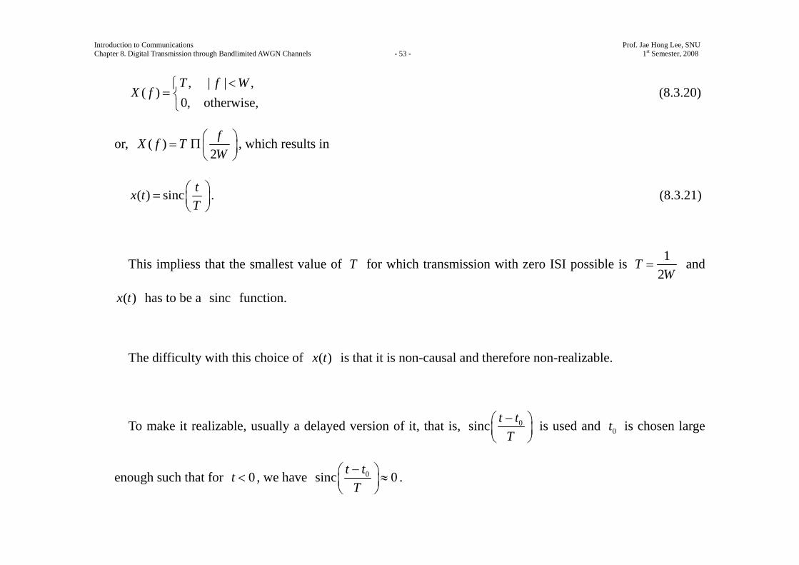
, | | ,( )
0, otherwise,T f W
X f<⎧
= ⎨⎩
(8.3.20)
or, ( )2fX f TW
⎛ ⎞= Π⎜ ⎟⎝ ⎠
, which results in
( ) sinc tx tT⎛ ⎞= ⎜ ⎟⎝ ⎠
. (8.3.21)
This impliess that the smallest value of T for which transmission with zero ISI possible is 12
TW
= and
( )x t has to be a sinc function.
The difficulty with this choice of ( )x t is that it is non-causal and therefore non-realizable.
To make it realizable, usually a delayed version of it, that is, 0sinc t tT−⎛ ⎞
⎜ ⎟⎝ ⎠
is used and 0t is chosen large
enough such that for 0t < , we have 0sinc 0t tT−⎛ ⎞ ≈⎜ ⎟
⎝ ⎠.

Introduction to Communications Prof. Jae Hong Lee, SNU Chapter 8. Digital Transmission through Bandlimited AWGN Channels - 54 - 1st Semester, 2008
With this choice of ( )x t , the sampling time must also be shifted to 0mT t+ .
A second difficulty with this pulse shape is that its rate of convergence to zero is slow.
The tails of ( )x t decay as 1t
, consequently, a small mistiming error in sampling the output of the matched
filter at the demodulator results in an infinite series of ISI components.
Such a series is not absolutely summable because of the 1t
rate of decay of the pulse and, hence, the sum of
the resulting ISI does not converge.
3. For 12
TW
> , ( )Z f consists of overlapping replications of ( )X f separated by 1T
, as shown in Figure
8.10.
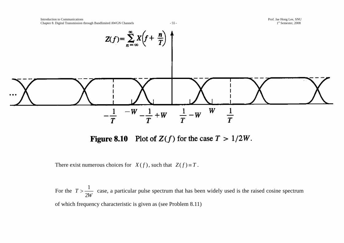
Introduction to Communications Prof. Jae Hong Lee, SNU Chapter 8. Digital Transmission through Bandlimited AWGN Channels - 55 - 1st Semester, 2008
There exist numerous choices for ( )X f , such that ( )Z f T≡ .
For the 12
TW
> case, a particular pulse spectrum that has been widely used is the raised cosine spectrum
of which frequency characteristic is given as (see Problem 8.11)
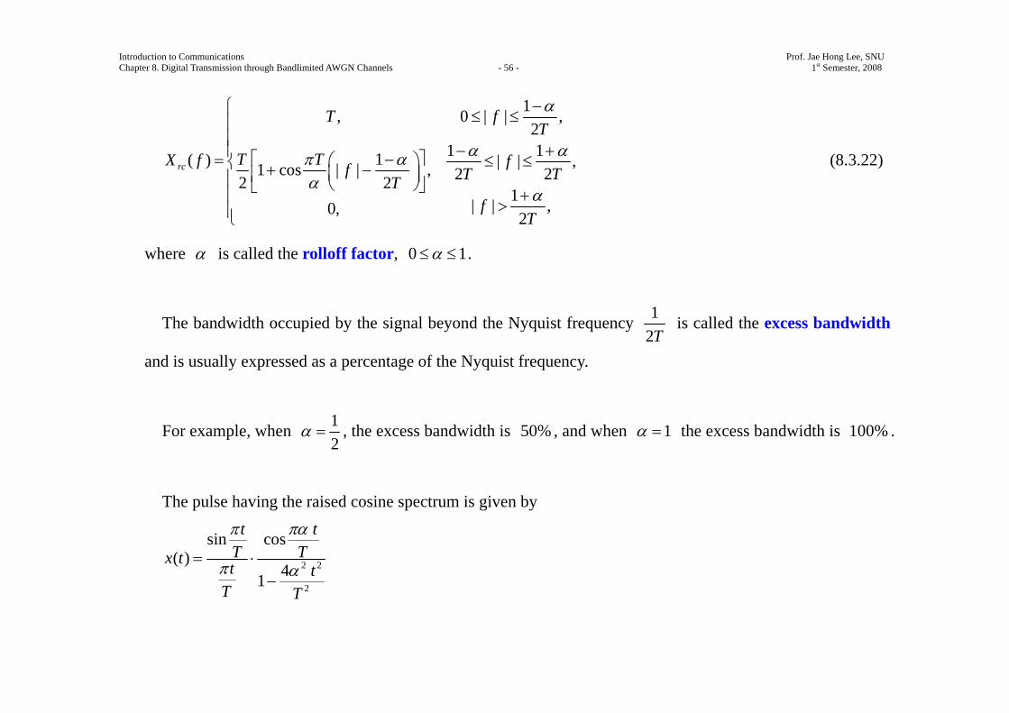
Introduction to Communications Prof. Jae Hong Lee, SNU Chapter 8. Digital Transmission through Bandlimited AWGN Channels - 56 - 1st Semester, 2008
1, 0 | | ,2
1 11( ) | | ,1 cos | | , 2 22 21| | ,0, 2
rc
T fT
T TX f ff T TTf
T
α
α απ αα
α
−⎧ ≤ ≤⎪⎪⎪ − +⎡ − ⎤= ⎛ ⎞ ≤ ≤⎨ + −⎜ ⎟⎢ ⎥⎪ ⎝ ⎠⎣ ⎦⎪ +
>⎪⎩
(8.3.22)
where α is called the rolloff factor, 0 1α≤ ≤ .
The bandwidth occupied by the signal beyond the Nyquist frequency 12T
is called the excess bandwidth
and is usually expressed as a percentage of the Nyquist frequency.
For example, when 12
α = , the excess bandwidth is 50% , and when 1α = the excess bandwidth is 100% .
The pulse having the raised cosine spectrum is given by
2 2
2
sin cos( )
41
t tT Tx t t t
T T
π πα
π α= ⋅
−
Introduction to Communications Prof. Jae Hong Lee, SNU Chapter 8. Digital Transmission through Bandlimited AWGN Channels - 57 - 1st Semester, 2008
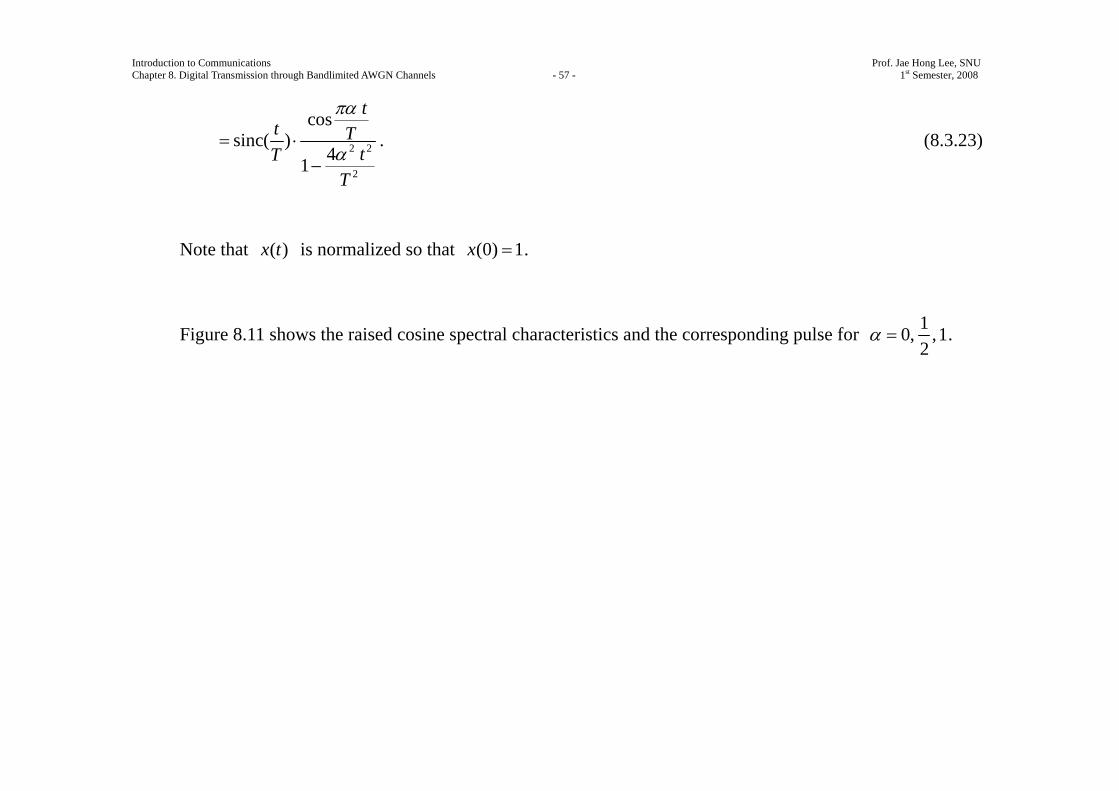
2 2
2
cossinc( )
41
tt T
tTT
πα
α= ⋅
−. (8.3.23)
Note that ( )x t is normalized so that (0) 1x = .
Figure 8.11 shows the raised cosine spectral characteristics and the corresponding pulse for 10, ,12
α = .

Introduction to Communications Prof. Jae Hong Lee, SNU Chapter 8. Digital Transmission through Bandlimited AWGN Channels - 58 - 1st Semester, 2008
Figure 8.11 Pulses having a raised cosine spectrum.
Introduction to Communications Prof. Jae Hong Lee, SNU Chapter 8. Digital Transmission through Bandlimited AWGN Channels - 59 - 1st Semester, 2008
Note that for 0α = , the pulse reduces to ( ) sinc tx tT⎛ ⎞= ⎜ ⎟⎝ ⎠
, and the symbol rate 1 2WT= .
When 1α = , the symbol rate is 1 WT= .
In general, the tails of ( )x t decay as 3
1t
for 0α > .
Consequently, a mistiming error in sampling leads to a series of intersymbol interference components that
converges to a finite value.
Thanks to smooth characteristics of the raised cosine spectrum, it is possible to design practical filters for
the transmitter and receiver that approximate the overall desired frequency responseing filter
In this case, if the receiver filter is matched to the transmitting filter, we have
( ) ( ) ( )rc T RX f G f G f=
2| ( ) |TG f= .
Introduction to Communications Prof. Jae Hong Lee, SNU Chapter 8. Digital Transmission through Bandlimited AWGN Channels - 60 - 1st Semester, 2008
Ideally,
02( ) | ( ) | j f tT rcG f X f e π−= (8.3.25)
and *( ) ( )R TG f G f= ,
where 0t is some nominal delay that is required to assure physical realizability of the filter.
Thus, the overall raised cosine spectral characteristic is split evenly between the transmitting filter and the
receiving filter.
Also note that an additional delay is necessary to ensure the physical realizability of the receiving filter.
Introduction to Communications Prof. Jae Hong Lee, SNU Chapter 8. Digital Transmission through Bandlimited AWGN Channels - 61 - 1st Semester, 2008
8.3.2 Design of Bandlimited Signals with Controlled ISI-Partial Response Signals
To achieve zero ISI, it is necessary to reduce the symbol rate 1T
below the Nyquist rate of 2W symbols/sec
in order to realize practical transmitting and receiving filters.
By relaxing the condition of zero ISI that ( ) 0x nT = for 0n ≠ , we can achieve a symbol transmission rate
of 2W symbols/sec.
Suppose that we design the bandlimited signal to have controlled ISI at one time instant which implies that
we allow one additional nonzero value in the samples { ( )}x nT .
The ISI that we introduce is deterministic or “controlled” and, hence, it can be taken into account at the
receiver.
Introduction to Communications Prof. Jae Hong Lee, SNU Chapter 8. Digital Transmission through Bandlimited AWGN Channels - 62 - 1st Semester, 2008
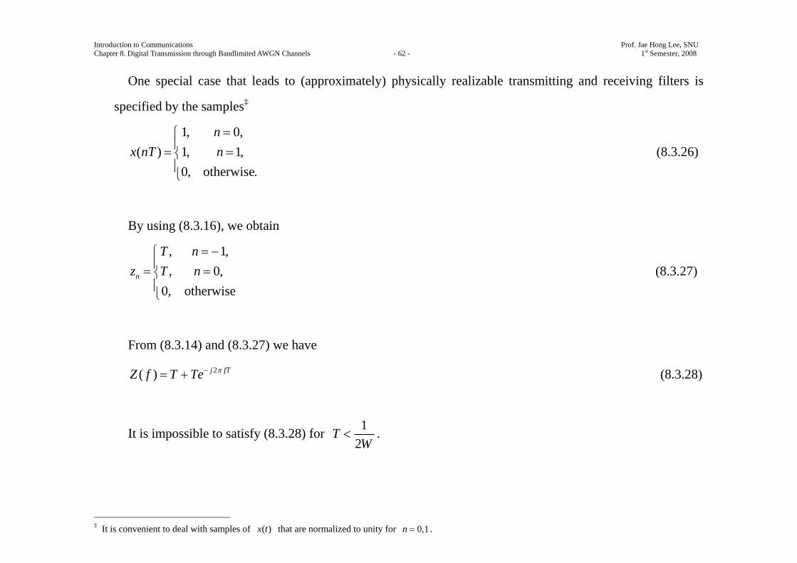
One special case that leads to (approximately) physically realizable transmitting and receiving filters is
specified by the samples‡
1, 0,( ) 1, 1,
0, otherwise.
nx nT n
=⎧⎪= =⎨⎪⎩
(8.3.26)
By using (8.3.16), we obtain
, 1,, 0,
0, otherwisen
T nz T n
= −⎧⎪= =⎨⎪⎩
(8.3.27)
From (8.3.14) and (8.3.27) we have
2( ) j fTZ f T Te π−= + (8.3.28)
It is impossible to satisfy (8.3.28) for 12
TW
< .
‡ It is convenient to deal with samples of ( )x t that are normalized to unity for 0,1n = .
Introduction to Communications Prof. Jae Hong Lee, SNU Chapter 8. Digital Transmission through Bandlimited AWGN Channels - 63 - 1st Semester, 2008
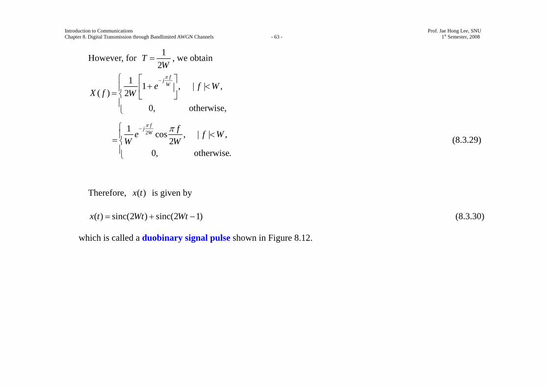
However, for 12
TW
= , we obtain
1 1 , | | ,( ) 2
0, otherwise,
fjWe f W
X f W
π−⎧ ⎡ ⎤
+ <⎪ ⎢ ⎥= ⎨ ⎣ ⎦⎪⎩
21 cos , | | ,2
0, otherwise.
fjW fe f W
W W
π π−⎧<⎪= ⎨
⎪⎩
(8.3.29)
Therefore, ( )x t is given by
( ) sinc(2 ) sinc(2 1)x t Wt Wt= + − (8.3.30)
which is called a duobinary signal pulse shown in Figure 8.12.
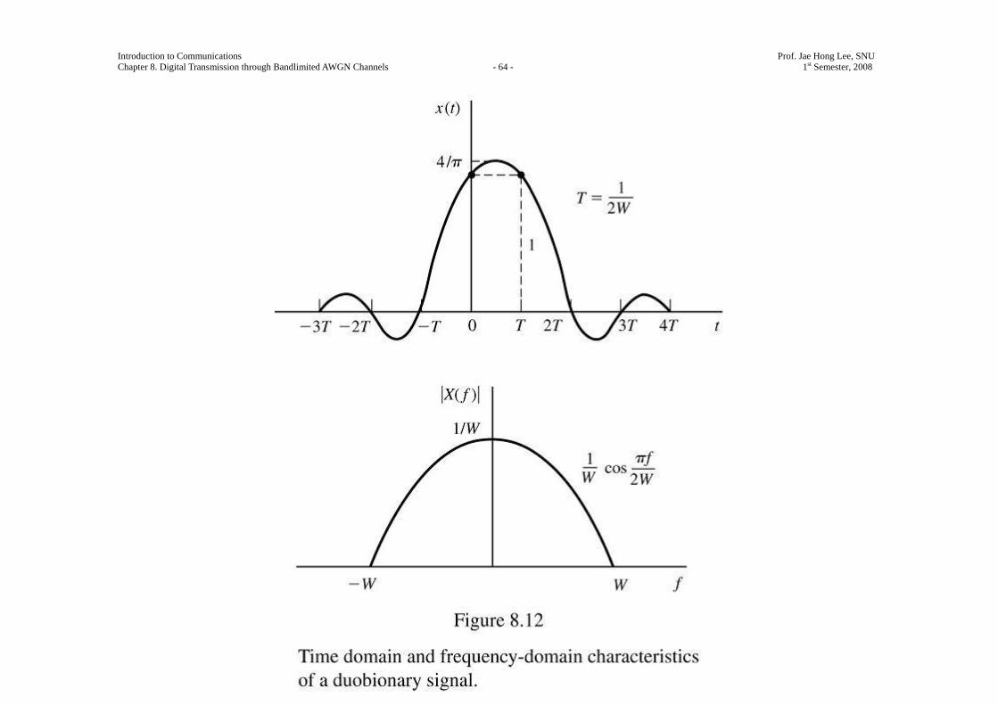
Introduction to Communications Prof. Jae Hong Lee, SNU Chapter 8. Digital Transmission through Bandlimited AWGN Channels - 64 - 1st Semester, 2008
Introduction to Communications Prof. Jae Hong Lee, SNU Chapter 8. Digital Transmission through Bandlimited AWGN Channels - 65 - 1st Semester, 2008
Note that the spectraum decays to zero smoothly, which means that physically realizable filters can be
designed that approximate this spectrum very closely.
Thus, a symbol rate of 2W is achieved.
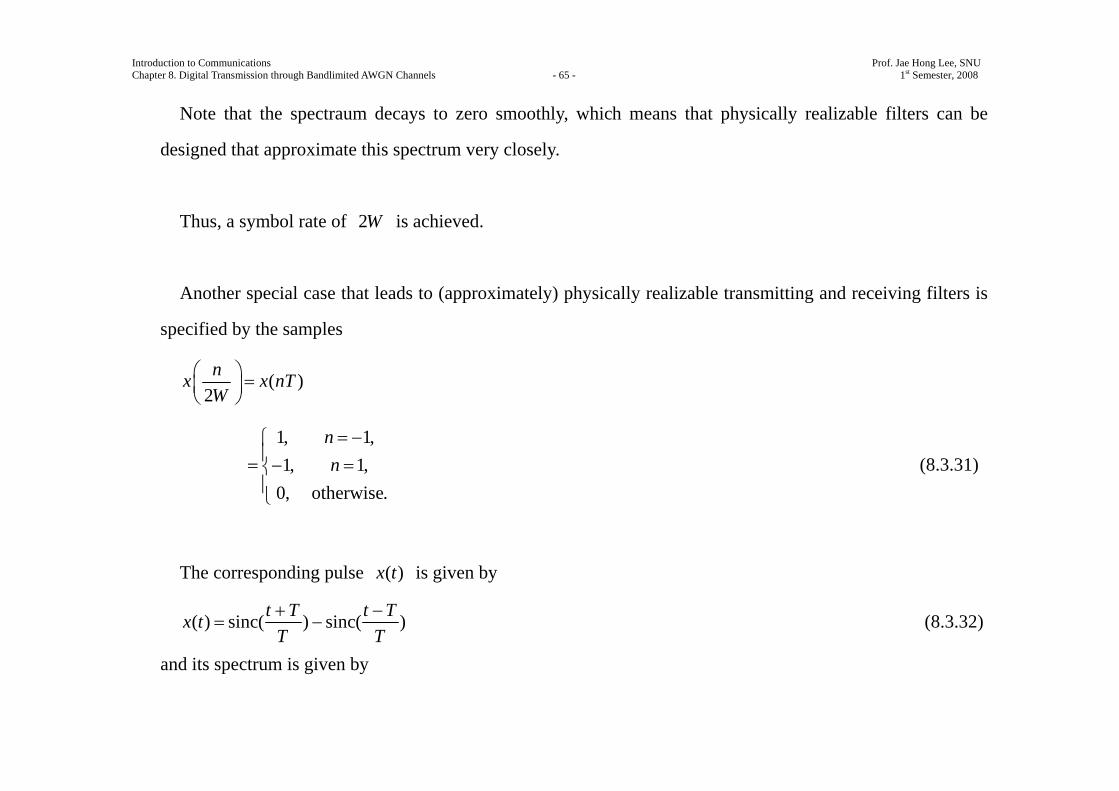
Another special case that leads to (approximately) physically realizable transmitting and receiving filters is
specified by the samples
( )2nx x nTW
⎛ ⎞ =⎜ ⎟⎝ ⎠
1, 1,1, 1,
0, otherwise.
nn= −⎧
⎪= − =⎨⎪⎩
(8.3.31)
The corresponding pulse ( )x t is given by
( ) sinc( ) sinc( )t T t Tx tT T+ −
= − (8.3.32)
and its spectrum is given by
Introduction to Communications Prof. Jae Hong Lee, SNU Chapter 8. Digital Transmission through Bandlimited AWGN Channels - 66 - 1st Semester, 2008
1 , | | ,( ) 20, | | ,
f fj jW We e f WX f W
f W
π π⎧− ≤⎪= ⎨
⎪ >⎩
sin , | | ,
0, | | ,
j f f WW W
f W
π⎧ ≤⎪= ⎨⎪ >⎩
(8.3.33)
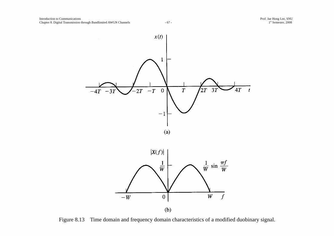
which is shown in Figure 8.13.
It is called a modified duobinary signal pulse.
Note that the spectrum of this signal has a zero at 0f = , making it suitable for transmission over a channel
that does not pass D.C.
Introduction to Communications Prof. Jae Hong Lee, SNU Chapter 8. Digital Transmission through Bandlimited AWGN Channels - 67 - 1st Semester, 2008
Figure 8.13 Time domain and frequency domain characteristics of a modified duobinary signal.
Introduction to Communications Prof. Jae Hong Lee, SNU Chapter 8. Digital Transmission through Bandlimited AWGN Channels - 68 - 1st Semester, 2008
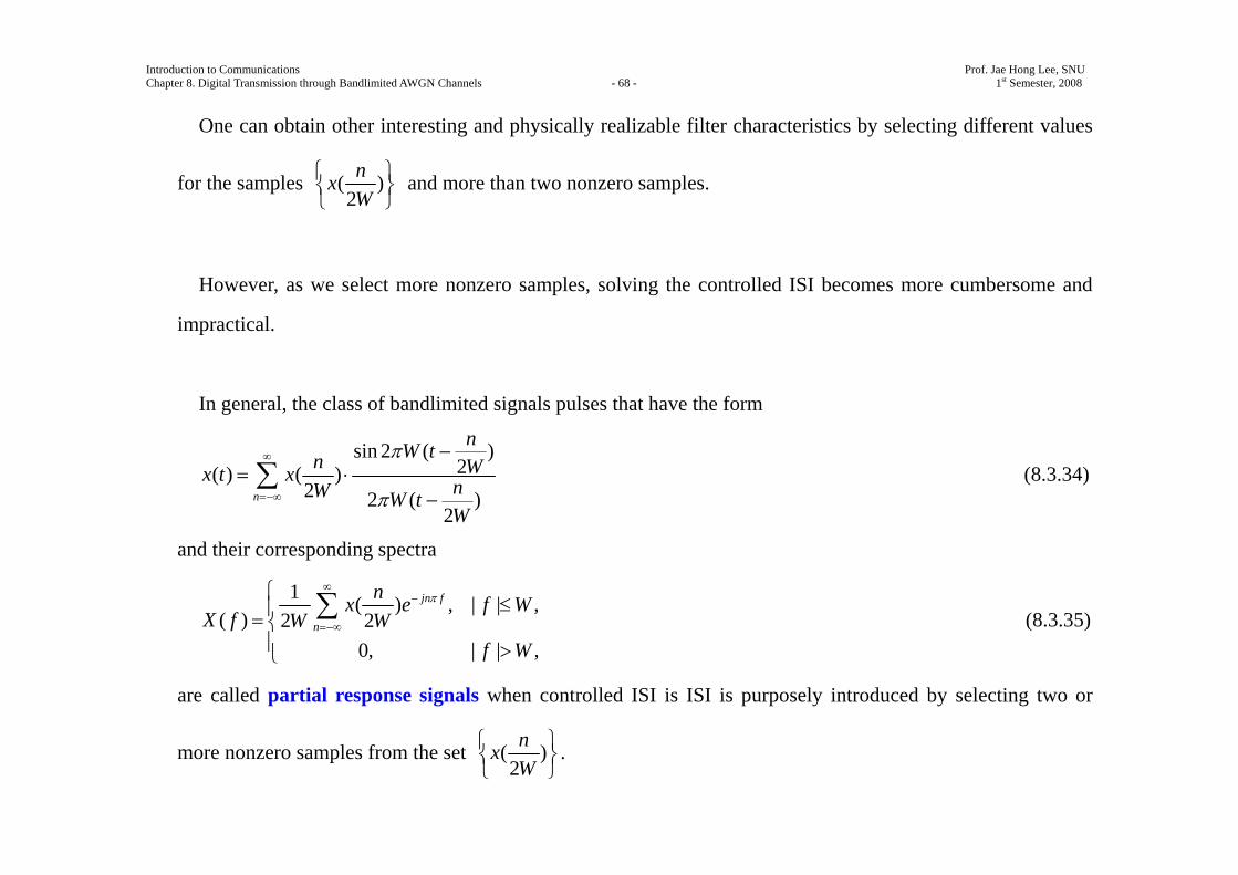
One can obtain other interesting and physically realizable filter characteristics by selecting different values
for the samples ( )2nxW
⎧ ⎫⎨ ⎬⎩ ⎭
and more than two nonzero samples.
However, as we select more nonzero samples, solving the controlled ISI becomes more cumbersome and
impractical.
In general, the class of bandlimited signals pulses that have the form
sin 2 ( )2( ) ( )
2 2 ( )2
n
nW tn Wx t x nW W tW
π
π
∞
=−∞
−= ⋅
−∑ (8.3.34)
and their corresponding spectra
1 ( ) , | | ,( ) 2 2
0, | | ,
jn f
n
nx e f WX f W W
f W
π∞
−
=−∞
⎧≤⎪= ⎨
⎪ >⎩
∑ (8.3.35)
are called partial response signals when controlled ISI is ISI is purposely introduced by selecting two or
more nonzero samples from the set ( )2nxW
⎧ ⎫⎨ ⎬⎩ ⎭
.
Introduction to Communications Prof. Jae Hong Lee, SNU Chapter 8. Digital Transmission through Bandlimited AWGN Channels - 69 - 1st Semester, 2008
The resulting signal pulses allow us to transmit information symbols at the Nyquist rate of 2W symbols
per second.
8.4 Probability of Error in Detection of PAM
We evaluate the performance of the receiver for demodulating and detecting an M -ary PAM signal in the
presence of additive white Gaussian noise at its input for two cases:
1) the case that the transmitting and receiving filters ( )TG f and ( )RG f are designed for zero ISI and
2) the case that ( )TG f and ( )RG f are designed such that ( ) ( ) ( )T Rx t g t g t= ∗ is either a duobinary signal
or a modified duobinary signal.
The results can be generalized to two-dimensional modulations, such as PSK and QAM, and
multidimensional signals.

Introduction to Communications Prof. Jae Hong Lee, SNU Chapter 8. Digital Transmission through Bandlimited AWGN Channels - 70 - 1st Semester, 2008
8.4.1 Probability of Error for Detection of PAM with Zero ISI
In the absence of ISI, the received signal sample at the output of the receiving matched filter is given by
0m m my x a v= + (8.4.1)
where
20 | ( ) |
W
TWx G f df
−= ∫
gε= (8.4.2)
and mv is the additive Gaussian noise which has zero mean and variance
02
2g
v
Nεσ = . (8.4.3)
Suppose that ma takes one of M possible equally spaced amplitude values with equal probability.
Then, the probability of error for digital PAM in a bandlimited additive white Gaussian noise channel in the
absence of ISI is identical to that for M -ary PAM as given in Section 7.6.2.
Introduction to Communications Prof. Jae Hong Lee, SNU Chapter 8. Digital Transmission through Bandlimited AWGN Channels - 71 - 1st Semester, 2008
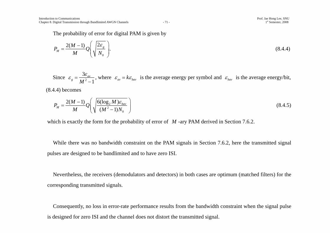
The probability of error for digital PAM is given by
0
22( 1) gM
MP QM N
ε⎛ ⎞−= ⎜ ⎟⎜ ⎟
⎝ ⎠. (8.4.4)
Since 2
31
avg M
εε =−
, where av bavkε ε= is the average energy per symbol and bavε is the average energy/bit,
(8.4.4) becomes
22
0
2( 1) 6(log )( 1)
bavM
M MP QM M N
ε⎛ ⎞−= ⎜ ⎟⎜ ⎟−⎝ ⎠
(8.4.5)
which is exactly the form for the probability of error of M -ary PAM derived in Section 7.6.2.
While there was no bandwidth constraint on the PAM signals in Section 7.6.2, here the transmitted signal
pulses are designed to be bandlimited and to have zero ISI.
Nevertheless, the receivers (demodulators and detectors) in both cases are optimum (matched filters) for the
corresponding transmitted signals.
Consequently, no loss in error-rate performance results from the bandwidth constraint when the signal pulse
is designed for zero ISI and the channel does not distort the transmitted signal.
Introduction to Communications Prof. Jae Hong Lee, SNU Chapter 8. Digital Transmission through Bandlimited AWGN Channels - 72 - 1st Semester, 2008
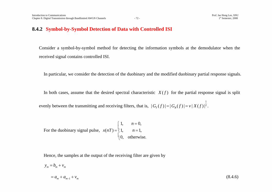
8.4.2 Symbol-by-Symbol Detection of Data with Controlled ISI
Consider a symbol-by-symbol method for detecting the information symbols at the demodulator when the
received signal contains controlled ISI.
In particular, we consider the detection of the duobinary and the modified duobinary partial response signals.
In both cases, assume that the desired spectral characteristic ( )X f for the partial response signal is split
evenly between the transmitting and receiving filters, that is, 12| ( ) | | ( ) | | ( ) |T RG f G f v X f= = .
For the duobinary signal pulse, 1, 0,
( ) 1, 1,0, otherwise.
nx nT n
=⎧⎪= =⎨⎪⎩
Hence, the samples at the output of the receiving filter are given by
m m my b v= +
1m m ma a v−= + + (8.4.6)
Introduction to Communications Prof. Jae Hong Lee, SNU Chapter 8. Digital Transmission through Bandlimited AWGN Channels - 73 - 1st Semester, 2008
where { }ma is the transmitted sequence of amplitudes and
{ }mv is a sequence of additive Gaussian noise samples.
Ignore the noise for the moment and consider the binary case where 1ma = ± with equal probability.
Then, mb takes on one of three possible values, namely, 2, 0, 2mb = − with corresponding probabilities
1 1 1, ,4 2 4
.
If the detected symbol from the ( 1)m − st signaling interval is 1ma − , its effect on the received signal in the
m th signaling interval mb can be eliminated by subtraction, thus allowing ma to be detected.
This process can be repeated sequentially for every received symbol.
The major problem with this procedure is that errors arising from the additive noise tend to propagate.
That is, if 1ma − is in error, its effect on mb is not eliminated but, in fact, it is reinforced by the incorrect
Introduction to Communications Prof. Jae Hong Lee, SNU Chapter 8. Digital Transmission through Bandlimited AWGN Channels - 74 - 1st Semester, 2008
subtraction so that the detection of ma is also likely to be in error.
Error propagation can be avoided by precoding the data on the binary data sequence prior to modulation at
the transmitter instead of eliminating the controlled ISI by subtraction at the receiver.
From the data sequence { }nd of 1’s and 0’s that is to be transmitted, a new sequence { }np , called the
precoded sequence, is generated.
For the duobinary signal, the precoded sequence is given by
m mp d= 1, 1, 2,mp m− = , (8.4.7)
where denotes modulo- 2 subtraction.†
Then, set 1ma = − if 0mp = and 1ma = if 1mp = , that is, 2 1m ma p= − .
The noise-free samples at the output of the receiving filter are given by
† Although this is identical to modulo-2 addition, it is convenient to view the precoding operation for duobinary in terms of modulo-2 subtraction.
Introduction to Communications Prof. Jae Hong Lee, SNU Chapter 8. Digital Transmission through Bandlimited AWGN Channels - 75 - 1st Semester, 2008
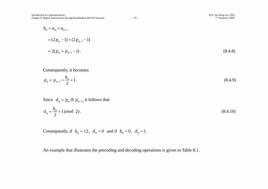
1m m mb a a −= +
1(2 1) (2 1)m mp p −= − + −
12( 1)m mp p −= + − . (8.4.8)
Consequently, it becomes
1 12m
m mbp p −+ = + . (8.4.9)
Since 1m m md p p −= ⊕ , it follows that
1 (mod 2)2m
mbd = + . (8.4.10)
Consequently, if 2mb = ± , 0md = and if 0mb = , 1md = .
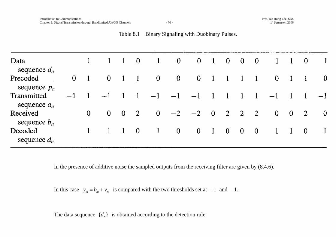
An example that illustrates the precoding and decoding operations is given in Table 8.1.
Introduction to Communications Prof. Jae Hong Lee, SNU Chapter 8. Digital Transmission through Bandlimited AWGN Channels - 76 - 1st Semester, 2008
Table 8.1 Binary Signaling with Duobinary Pulses.
In the presence of additive noise the sampled outputs from the receiving filter are given by (8.4.6).
In this case m m my b v= + is compared with the two thresholds set at 1+ and 1− .
The data sequence { }nd is obtained according to the detection rule
Introduction to Communications Prof. Jae Hong Lee, SNU Chapter 8. Digital Transmission through Bandlimited AWGN Channels - 77 - 1st Semester, 2008
1, 1 1,0, | | 1.
mm
m
yd
y− < <⎧
= ⎨ ≥⎩ (8.4.11)
The extension from binary PAM to multilevel PAM signaling using the duobinary pulse is straightforward.
In this case the M -level amplitude sequence { }ma results in a (noise-free) sequence
1m m mb a a −= + , 1, 2, ,m = (8.4.12)
which has 2 1M − possible equally spaced levels.
The amplitude levels are determined from the relation
2 ( 1)m ma p M= − − (8.4.13)
where { }mp is the precoded sequence that is obtained from an M -level data sequence { }md according to
the relation (see (8.4.7))
m mp d= 1(mod )mp M− (8.4.14)
where denotes modulo- M subtraction and the possible values of the sequence { }md are 0,1, 2, , 1M − .
Introduction to Communications Prof. Jae Hong Lee, SNU Chapter 8. Digital Transmission through Bandlimited AWGN Channels - 78 - 1st Semester, 2008
In the absence of noise, the samples at the output of the receiving filter are expressed as
1m m mb a a −= +
12[ ( 1)]m mp p M−= + − − . (8.4.15)
Hence,
1 ( 1)2m
m mbp p M−+ = + − . (8.4.16)
Since 1 (mod )m m md p p M−= + , it follows that
( 1)2m
mbd M= + − (mod )M . (8.4.17)
An example illustrating multilevel precoding and decoding is given in Table 8.2.
Introduction to Communications Prof. Jae Hong Lee, SNU Chapter 8. Digital Transmission through Bandlimited AWGN Channels - 79 - 1st Semester, 2008
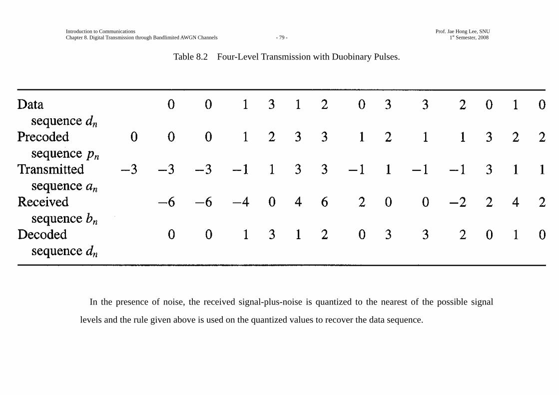
Table 8.2 Four-Level Transmission with Duobinary Pulses.
In the presence of noise, the received signal-plus-noise is quantized to the nearest of the possible signal
levels and the rule given above is used on the quantized values to recover the data sequence.
Introduction to Communications Prof. Jae Hong Lee, SNU Chapter 8. Digital Transmission through Bandlimited AWGN Channels - 80 - 1st Semester, 2008
In the case of the modified duobinary pulse, the controlled ISI is given by
1, 1,( ) 1, 1,2
0, otherwise.
nnx nW
= −⎧⎪= − =⎨⎪⎩
Consequently, the noise-free sampled output from the receiving filter is given by
2m m mb a a −= − (8.4.18)
where the M -level sequence { }na is obtained by mapping a precoded sequence according to the relation
(8.2.43) and
2 (mod )m m mp d p M−= ⊕ . (8.4.19)
From these relations, it is shown that the detection rule for recovering the data sequence { }md from { }mb
in the absence of noise is given by
(mod )2m
mbd M= . (8.4.20)
Note that the precoding of the data at the transmitter makes it possible to detect the received data on a
symbol-by-symbol basis without having to look back at previously detected symbols.
Introduction to Communications Prof. Jae Hong Lee, SNU Chapter 8. Digital Transmission through Bandlimited AWGN Channels - 81 - 1st Semester, 2008
Thus, error propagation is avoided.
The symbol-by-symbol detection rule described above is not the optimum detection scheme for partial
response signals.
Nevertheless, symbol-by-symbol detection is relatively simple to implement and is used in many practical
applications involving duobinary and modified duobinary pulse signals.
Introduction to Communications Prof. Jae Hong Lee, SNU Chapter 8. Digital Transmission through Bandlimited AWGN Channels - 82 - 1st Semester, 2008
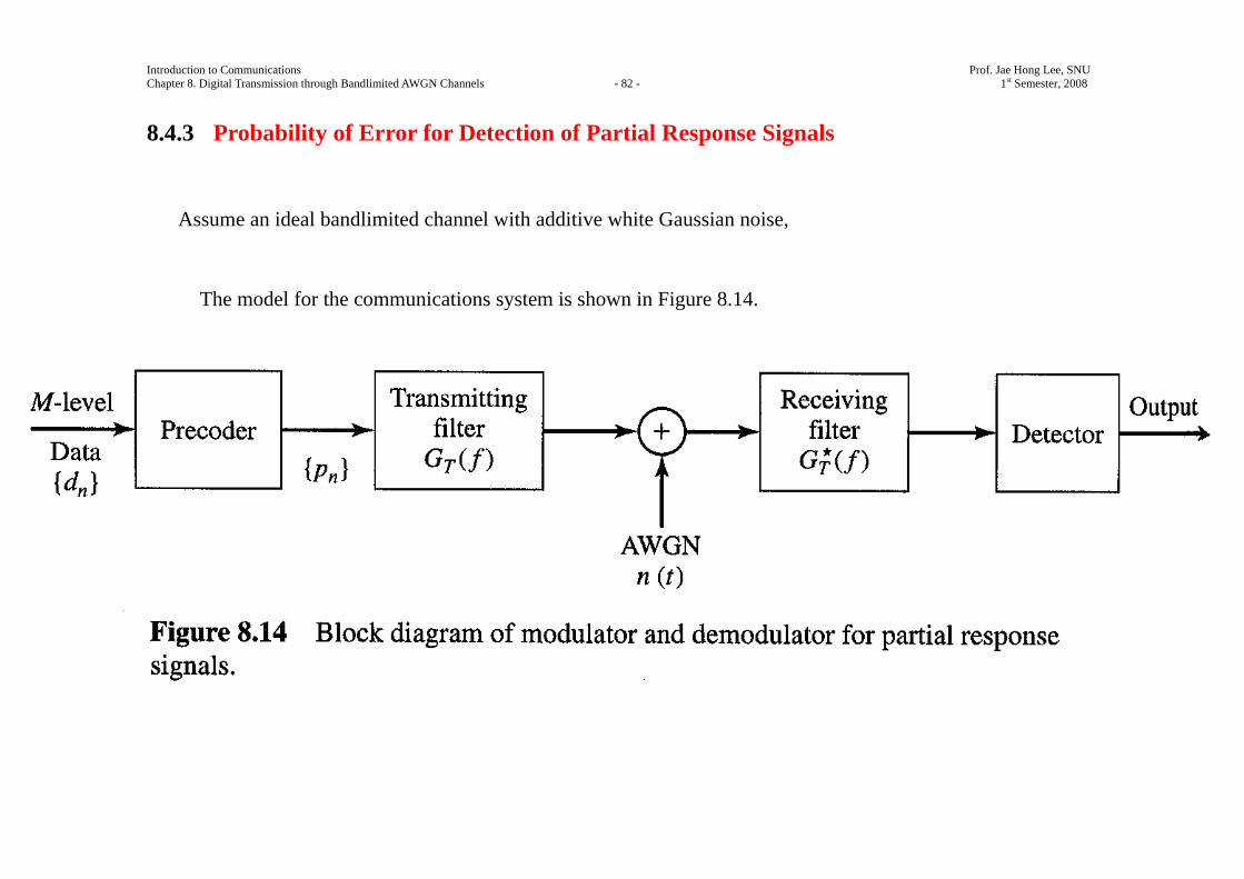
8.4.3 Probability of Error for Detection of Partial Response Signals
Assume an ideal bandlimited channel with additive white Gaussian noise,
The model for the communications system is shown in Figure 8.14.
Introduction to Communications Prof. Jae Hong Lee, SNU Chapter 8. Digital Transmission through Bandlimited AWGN Channels - 83 - 1st Semester, 2008
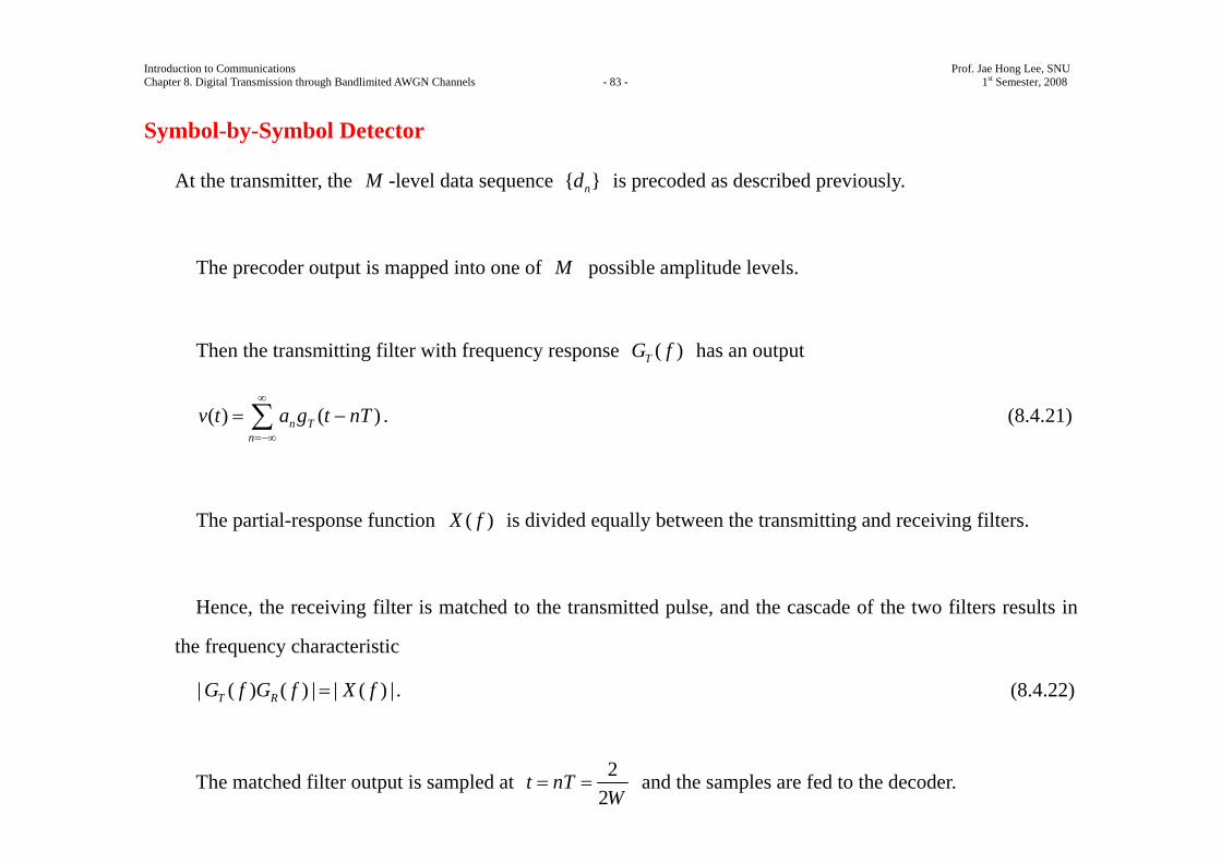
Symbol-by-Symbol Detector
At the transmitter, the M -level data sequence { }nd is precoded as described previously.
The precoder output is mapped into one of M possible amplitude levels.
Then the transmitting filter with frequency response ( )TG f has an output
( ) ( )n Tn
v t a g t nT∞
=−∞
= −∑ . (8.4.21)
The partial-response function ( )X f is divided equally between the transmitting and receiving filters.
Hence, the receiving filter is matched to the transmitted pulse, and the cascade of the two filters results in
the frequency characteristic
| ( ) ( ) | | ( ) |T RG f G f X f= . (8.4.22)
The matched filter output is sampled at 22
t nTW
= = and the samples are fed to the decoder.
Introduction to Communications Prof. Jae Hong Lee, SNU Chapter 8. Digital Transmission through Bandlimited AWGN Channels - 84 - 1st Semester, 2008
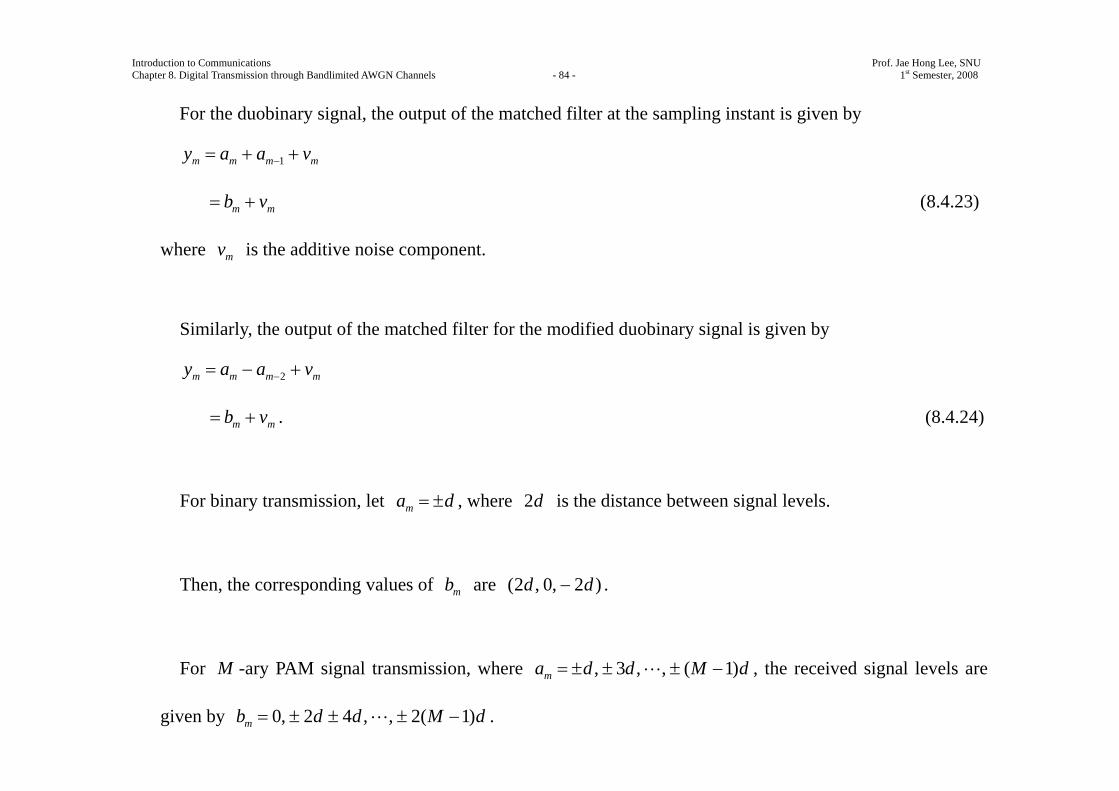
For the duobinary signal, the output of the matched filter at the sampling instant is given by
1m m m my a a v−= + +
m mb v= + (8.4.23)
where mv is the additive noise component.
Similarly, the output of the matched filter for the modified duobinary signal is given by
2m m m my a a v−= − +
m mb v= + . (8.4.24)
For binary transmission, let ma d= ± , where 2d is the distance between signal levels.
Then, the corresponding values of mb are (2 , 0, 2 )d d− .
For M -ary PAM signal transmission, where , 3 , , ( 1)ma d d M d= ± ± ± − , the received signal levels are
given by 0, 2 4 , , 2( 1)mb d d M d= ± ± ± − .
Introduction to Communications Prof. Jae Hong Lee, SNU Chapter 8. Digital Transmission through Bandlimited AWGN Channels - 85 - 1st Semester, 2008
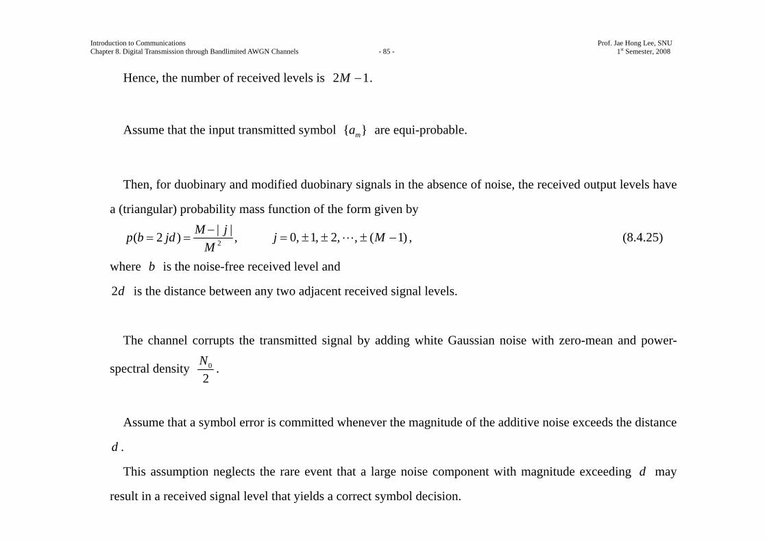
Hence, the number of received levels is 2 1M − .
Assume that the input transmitted symbol { }ma are equi-probable.
Then, for duobinary and modified duobinary signals in the absence of noise, the received output levels have
a (triangular) probability mass function of the form given by
2
| |( 2 ) M jp b jdM−
= = , 0, 1, 2, , ( 1)j M= ± ± ± − , (8.4.25)
where b is the noise-free received level and
2d is the distance between any two adjacent received signal levels.
The channel corrupts the transmitted signal by adding white Gaussian noise with zero-mean and power-
spectral density 0
2N .
Assume that a symbol error is committed whenever the magnitude of the additive noise exceeds the distance
d .
This assumption neglects the rare event that a large noise component with magnitude exceeding d may
result in a received signal level that yields a correct symbol decision.
Introduction to Communications Prof. Jae Hong Lee, SNU Chapter 8. Digital Transmission through Bandlimited AWGN Channels - 86 - 1st Semester, 2008
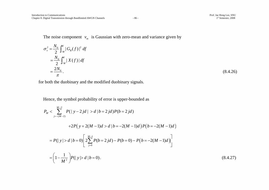
The noise component mv is Gaussian with zero-mean and variance given by
2 20 | ( ) |2
W
v RW
N G f dfσ−
= ∫
0 | ( ) |2
W
W
N X f df−
= ∫
02Nπ
= . (8.4.26)
for both the duobinary and the modified duobinary signals.
Hence, the symbol probability of error is upper-bounded as
2
( 2)( | 2 | | 2 ) ( 2 )
M
Mj M
P P y jd d b jd P b jd−
=− −
< − > = =∑
( ) ( )2 2( 1) | 2( 1) 2( 1)P y M d d b M d P b M d+ + − > = − − = − −
( )1
0
(| | | 0) 2 ( 2 ) ( 0) 2( 1)M
j
P y d b P b jd P b P b M d−
=
⎡ ⎤= > = = − = − = − −⎢ ⎥
⎣ ⎦∑
2
11 (| | | 0)P y d bM
⎛ ⎞= − > =⎜ ⎟⎝ ⎠
. (8.4.27)
Introduction to Communications Prof. Jae Hong Lee, SNU Chapter 8. Digital Transmission through Bandlimited AWGN Channels - 87 - 1st Semester, 2008
But 2
222(| | | 0)2
v
x
dv
P y d b e dxσ
πσ
−∞> = = ∫
2
0
22
dQN
π⎛ ⎞= ⎜ ⎟⎜ ⎟
⎝ ⎠. (8.4.28)
Therefore, the average probability of symbol error is upper-bounded as
2
20
12 12M
dP QM N
π⎛ ⎞⎛ ⎞< − ⎜ ⎟⎜ ⎟ ⎜ ⎟⎝ ⎠ ⎝ ⎠. (8.4.29)
For the M -ary PAM signal with equi-probable transmitted level, the average power at the output of the
transmitting filter is given by
22[ ] | ( ) |
Wm
av TW
E aP G f dfT −
= ∫
2[ ] | ( ) |W
mW
E a X f dfT −
= ∫
24 [ ]mE aTπ
= (8.4.30)
Introduction to Communications Prof. Jae Hong Lee, SNU Chapter 8. Digital Transmission through Bandlimited AWGN Channels - 88 - 1st Semester, 2008
where 2[ ]mE a is the mean square value of the M signal levels which is given by
2 22 ( 1)[ ]
3md ME a −
= . (8.4.31)
Therefore,
22
34( 1)
avP TdMπ
=−
. (8.4.32)
By plugging (8.4.32) into (8.4.29), the upper-bound for the symbol error probability is obtained as 2
2 20
1 62 14 1
avMP Q
M M Nπ ε⎛ ⎞⎛ ⎞ ⎛ ⎞⎜ ⎟< −⎜ ⎟ ⎜ ⎟⎜ ⎟−⎝ ⎠ ⎝ ⎠⎝ ⎠
(8.4.33)
where avε is the average energy/transmitted symbol, which can be also expressed in terms of the average bit
energy by 2(log )av bav bavk Mε ε ε= = .
(8.4.33) for the probability of error of M -ary PAM holds for both a duobinary and a modified duobinary
partial response signal.

Introduction to Communications Prof. Jae Hong Lee, SNU Chapter 8. Digital Transmission through Bandlimited AWGN Channels - 89 - 1st Semester, 2008
Comparing this result with the error probability of M -ary PAM with zero ISI which is obtained by using a
signal pulse with a raised cosine spectrum, we note that the performance of partial response duobinary or
modified duobinary has a loss of 2
4π⎛ ⎞⎜ ⎟⎝ ⎠
or 2.1 dB.
This loss in SNR is due to the fact that the detector for the partial response signals makes decisions on a
symbol-by-symbol basis, thus, ignoring the inherent memory contained in the received signal at the input to
the detector.
To observe the memory in the received sequence, look at the noise-free received sequence for binary
transmission given in Table 8.1.
Introduction to Communications Prof. Jae Hong Lee, SNU Chapter 8. Digital Transmission through Bandlimited AWGN Channels - 90 - 1st Semester, 2008
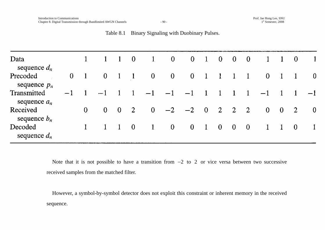
Table 8.1 Binary Signaling with Duobinary Pulses.
Note that it is not possible to have a transition from 2− to 2 or vice versa between two successive
received samples from the matched filter.
However, a symbol-by-symbol detector does not exploit this constraint or inherent memory in the received
sequence.
Introduction to Communications Prof. Jae Hong Lee, SNU Chapter 8. Digital Transmission through Bandlimited AWGN Channels - 91 - 1st Semester, 2008
8.5 Digitally Modulated Signals with Memory
The spectrum shaping obtained with partial response signals (in Section 8.3) can be viewed as resulting
from the memory introduced in the transmitted sequence of symbols, that is, the sequence of symbols are
correlated and, as a consequence, the power spectral density of the transmitted symbol sequence is colored
(nonwhite).
Signal dependence among signals transmitted in different signal intervals is generally accomplished by
encoding the data at the input to the modulator by means of a modulation code.
Introduction to Communications Prof. Jae Hong Lee, SNU Chapter 8. Digital Transmission through Bandlimited AWGN Channels - 92 - 1st Semester, 2008
8.5.1 Modulation Codes and Modulation Signals with Memory
Modulation codes are usually employed in magnetic recording, optical recording, and digital communications
over cable systems to achieve spectral shaping of the modulated signal that matches the passband
characteristics of the channel.
In magnetic recording we encounter two bais problems: 1) the packing density and 2) the dc content.
The first problem in magnetic recording is that we need to write as many bits as possible on a single track of
magnetic medium (disk or tape) to ahieve high packing density.
However, the medium imposes a limit on how closely successive bits in a sequence are stored.
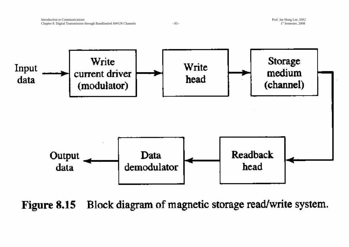
Figure 8.15 shows a block diagram of the magnetic recording system.
Introduction to Communications Prof. Jae Hong Lee, SNU Chapter 8. Digital Transmission through Bandlimited AWGN Channels - 93 - 1st Semester, 2008

Introduction to Communications Prof. Jae Hong Lee, SNU Chapter 8. Digital Transmission through Bandlimited AWGN Channels - 94 - 1st Semester, 2008
The binary input data sequence is used to generate a write current which can be viewed as the output of the
“modulator.”
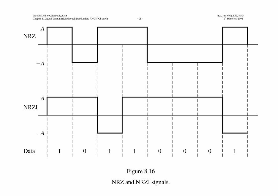
The two most commonly used methods to map the data sequence into the write current waveform are the
NRZ (non-return-to-zero) and NRZI (non-return-to-zero inverse) methods of which waveforms are shown in
Figure 8.16.
Introduction to Communications Prof. Jae Hong Lee, SNU Chapter 8. Digital Transmission through Bandlimited AWGN Channels - 95 - 1st Semester, 2008
Introduction to Communications Prof. Jae Hong Lee, SNU Chapter 8. Digital Transmission through Bandlimited AWGN Channels - 96 - 1st Semester, 2008
Note that NRZ is identical to binary PAM in which the information bit 1 is represented by a rectangular
pulse of amplitude A and the information bit 0 is represented by a rectangular pulse of amplitude A− .
In the NRZI, transitions from one amplitude level to another ( A to A− , or A− to A ) occur only when
the information bit is a 1.
In the NRZI, no transition occurs when the information bit is a 0 , that is, the amplitude level remains the
same as the previous signal level.
The positive amplitude pulse results in magnetizing the medium on one (direction) polarity and the negative
pulse magnetizes the medium in the opposite (direction) polarity.
Assume that the input data sequence is the sequence of independent random variables with equi-probable
1’s and 0’s.
Then, whether we use NRZ or NRZI, there are level transitions for A to A− or A− to A with
probability 12
(that is, each with probability 14
) for every data bit.

Introduction to Communications Prof. Jae Hong Lee, SNU Chapter 8. Digital Transmission through Bandlimited AWGN Channels - 97 - 1st Semester, 2008
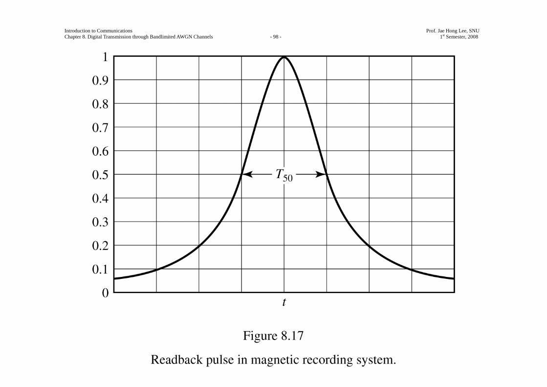
Suppose that the readback signal for a positive transition ( A− to A ) is a pulse modeled as
2
50
1( )21
p tt
T
=⎛ ⎞
+ ⎜ ⎟⎝ ⎠
(8.5.1)
where 50T is the width of the pulse at its 50% amplitude level as shown in Figure 8.17.
The value of 50T is determined by the characteristics of the medium and the read/write heads.
Then, the readback signal for a negative transition ( A to A− ) becomes the pulse ( )p t− .
Introduction to Communications Prof. Jae Hong Lee, SNU Chapter 8. Digital Transmission through Bandlimited AWGN Channels - 98 - 1st Semester, 2008
Introduction to Communications Prof. Jae Hong Lee, SNU Chapter 8. Digital Transmission through Bandlimited AWGN Channels - 99 - 1st Semester, 2008
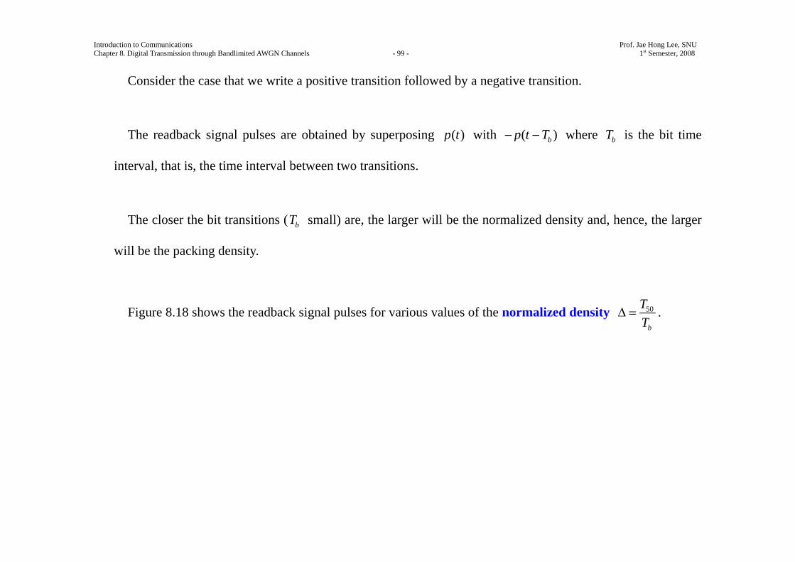
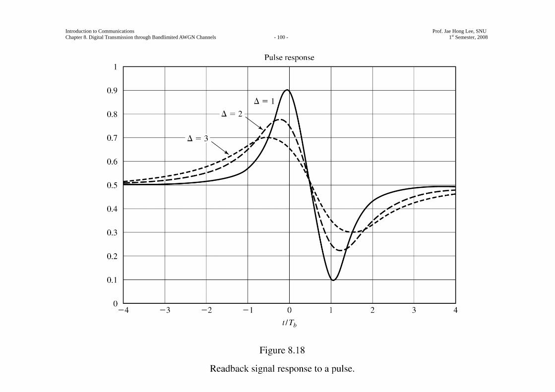
Consider the case that we write a positive transition followed by a negative transition.
The readback signal pulses are obtained by superposing ( )p t with ( )bp t T− − where bT is the bit time
interval, that is, the time interval between two transitions.
The closer the bit transitions ( bT small) are, the larger will be the normalized density and, hence, the larger
will be the packing density.
Figure 8.18 shows the readback signal pulses for various values of the normalized density 50
b
TT
Δ = .
Introduction to Communications Prof. Jae Hong Lee, SNU Chapter 8. Digital Transmission through Bandlimited AWGN Channels - 100 - 1st Semester, 2008
Introduction to Communications Prof. Jae Hong Lee, SNU Chapter 8. Digital Transmission through Bandlimited AWGN Channels - 101 - 1st Semester, 2008
Notice that as the normalized density Δ is increased, the peak amplitudes of the readback signal are
reduced and are shifted in time from the desired time instants.
This implies that the pulses interfere with each another, limiting the density with which we can write
transitions.
It needs to design modulation codes that take the original data sequence and transform (or encode) it into
another sequence which results in a write waveform having amplitude transitions spaced further apart.
For example, if we use NRZI, the encoded sequence into the modulator contains one or more 0’s between
1’s.
The second problem in magnetic recording is that we want to avoid (or minimize) having a dc component in
the modulated signal (the write current) because of the frequency-response characteristics of the readback
system and digital communication over cable channels.
This problem can also be overcome by altering (encoding) the data sequence to the modulator.
Introduction to Communications Prof. Jae Hong Lee, SNU Chapter 8. Digital Transmission through Bandlimited AWGN Channels - 102 - 1st Semester, 2008
A class of codes that solves these two problems are modulation codes.
Runlength-Limited Codes
Codes that have a restriction on the number of consecutive 1’s or 0’s in a sequence are generally called
runlength-limited codes.
These codes are generally described by two parameters: d and κ (‘kappa’),
where d is the minimum number of 0’s between 1’s in a sequence, and
κ is the maximum number of 0’s between two 1’s in a sequence.
When used with NRZI modulation, placing d zeros between successive 1’s spreads the transitions farther
apart, thus, reducing the overlap in the channel response due to successive transitions.
Setting an upper limit κ on the runlength of 0’s ensures that transitions occur frequently enough so that
symbol timing information can be recovered from the received modulated signal.
Introduction to Communications Prof. Jae Hong Lee, SNU Chapter 8. Digital Transmission through Bandlimited AWGN Channels - 103 - 1st Semester, 2008
Runlength-limited codes are usually called (d ,κ ) codes.†
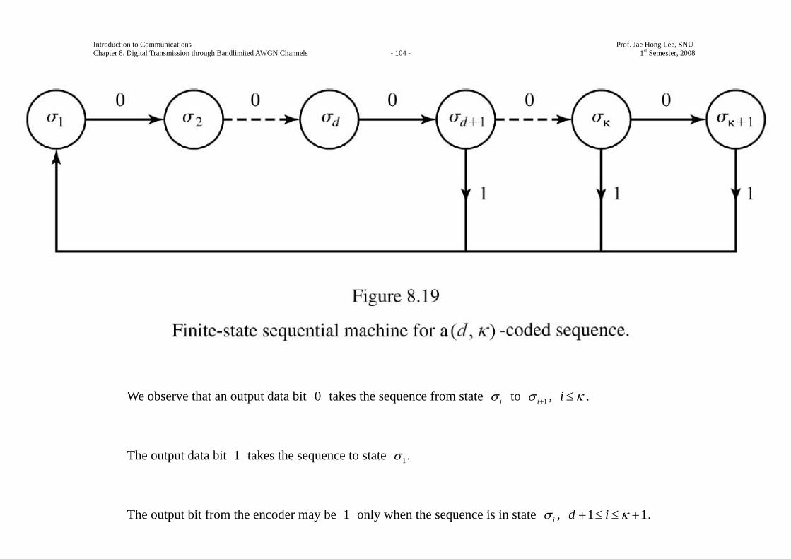
The ( d ,κ ) code sequence constraints may be represented by a finite-state sequential machine with 1κ +
states which is denoted by iσ , 1 1i κ≤ ≤ + , as shown in Figure 8.19.
† Runlength-limited codes are usually called ( d , k ) codes, where k is the maximum runlength of zeros. We have substituted the Greek letter κ for k , to avoid confusion with our previous use of k .
Introduction to Communications Prof. Jae Hong Lee, SNU Chapter 8. Digital Transmission through Bandlimited AWGN Channels - 104 - 1st Semester, 2008
We observe that an output data bit 0 takes the sequence from state iσ to 1iσ + , i κ≤ .
The output data bit 1 takes the sequence to state 1σ .
The output bit from the encoder may be 1 only when the sequence is in state iσ , 1 1d i κ+ ≤ ≤ + .
Introduction to Communications Prof. Jae Hong Lee, SNU Chapter 8. Digital Transmission through Bandlimited AWGN Channels - 105 - 1st Semester, 2008
When the sequence is in state 1κσ + , the output bit is always 1.
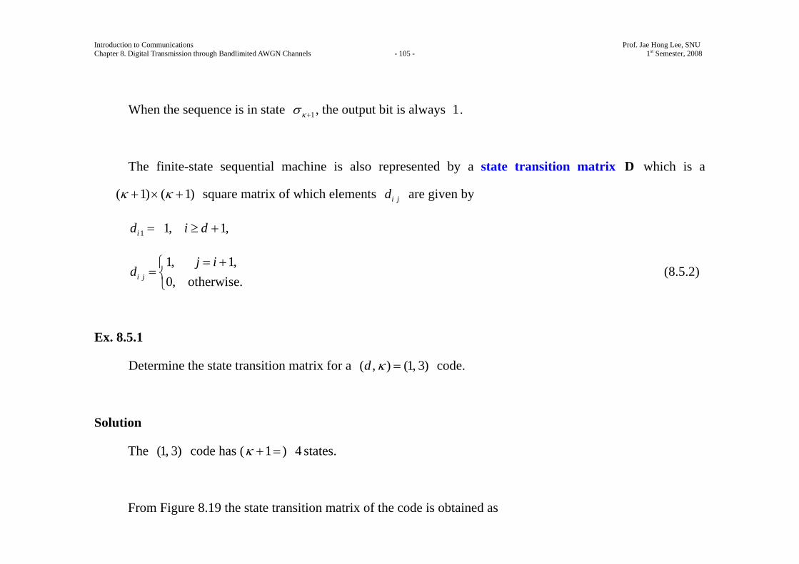
The finite-state sequential machine is also represented by a state transition matrix D which is a
( 1) ( 1)κ κ+ × + square matrix of which elements i jd are given by
1 1, 1,id i d= ≥ +
1, 1,0, otherwise.i j
j id
= +⎧= ⎨⎩
(8.5.2)
Ex. 8.5.1
Determine the state transition matrix for a ( , ) (1, 3)d κ = code.
Solution
The (1, 3) code has ( 1κ + = ) 4 states.
From Figure 8.19 the state transition matrix of the code is obtained as
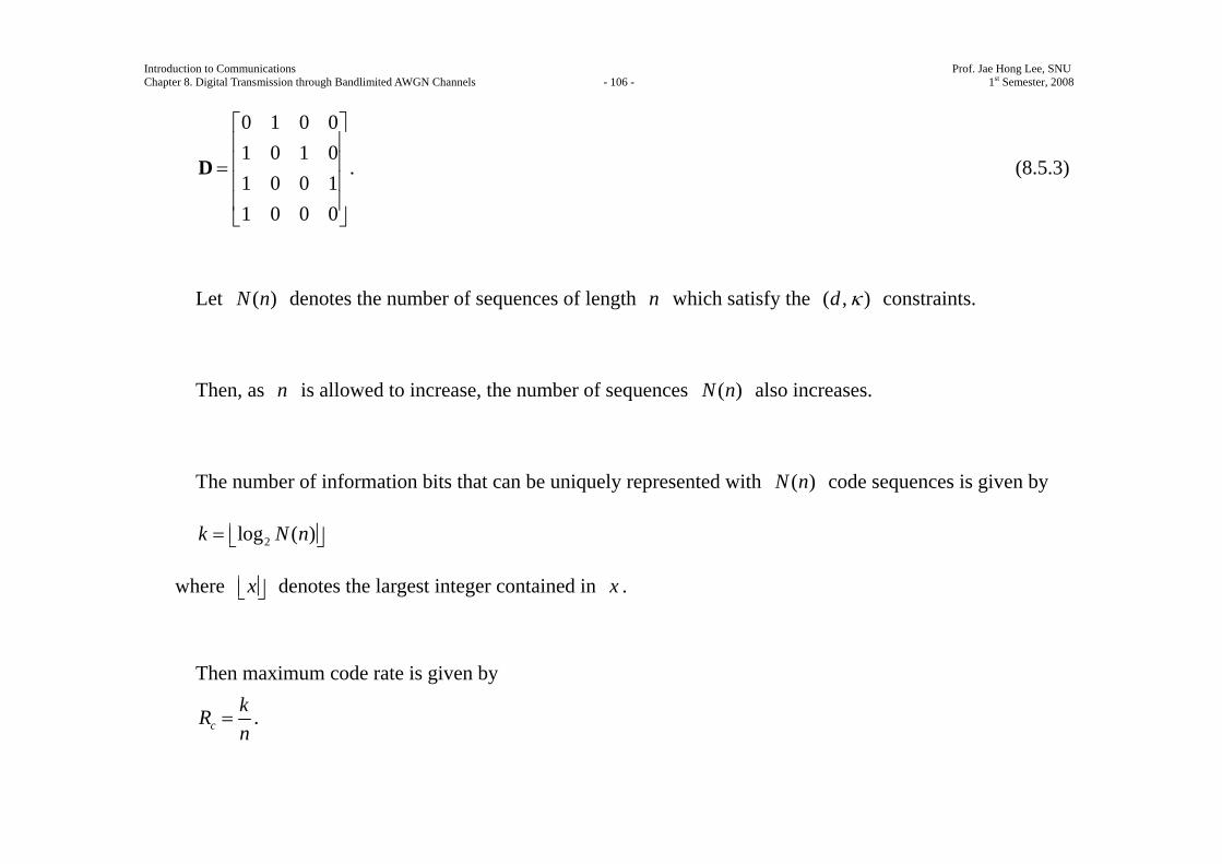
Introduction to Communications Prof. Jae Hong Lee, SNU Chapter 8. Digital Transmission through Bandlimited AWGN Channels - 106 - 1st Semester, 2008
0 1 0 01 0 1 01 0 0 11 0 0 0
⎡ ⎤⎢ ⎥⎢ ⎥=⎢ ⎥⎢ ⎥⎣ ⎦
D . (8.5.3)
Let ( )N n denotes the number of sequences of length n which satisfy the ( , )d κ constraints.
Then, as n is allowed to increase, the number of sequences ( )N n also increases.
The number of information bits that can be uniquely represented with ( )N n code sequences is given by
2log ( )k N n= ⎢ ⎥⎣ ⎦
where x⎢ ⎥⎣ ⎦ denotes the largest integer contained in x .
Then maximum code rate is given by
ckRn
= .
Introduction to Communications Prof. Jae Hong Lee, SNU Chapter 8. Digital Transmission through Bandlimited AWGN Channels - 107 - 1st Semester, 2008
The capacity of a ( , )d κ code is defined as
21( , ) lim log ( )
nC d N n
nκ
→∞= . (8.5.4)
which is the maximum possible rate that can be achieved with the ( , )d κ constraints.
Shannon (1948) showed that the capacity the ( , )d κ code is given by
2 max( , ) logC d κ λ= (8.5.5)
where maxλ is the largest real eigenvalue of the state transition matrix D the code.
Ex. 8.5.2
Determine the capacity of a ( , ) (1, 3)d κ = code.
Solution
Using the state-transition matrix given in Example 8.5.1 for the (1, 3) code, we have
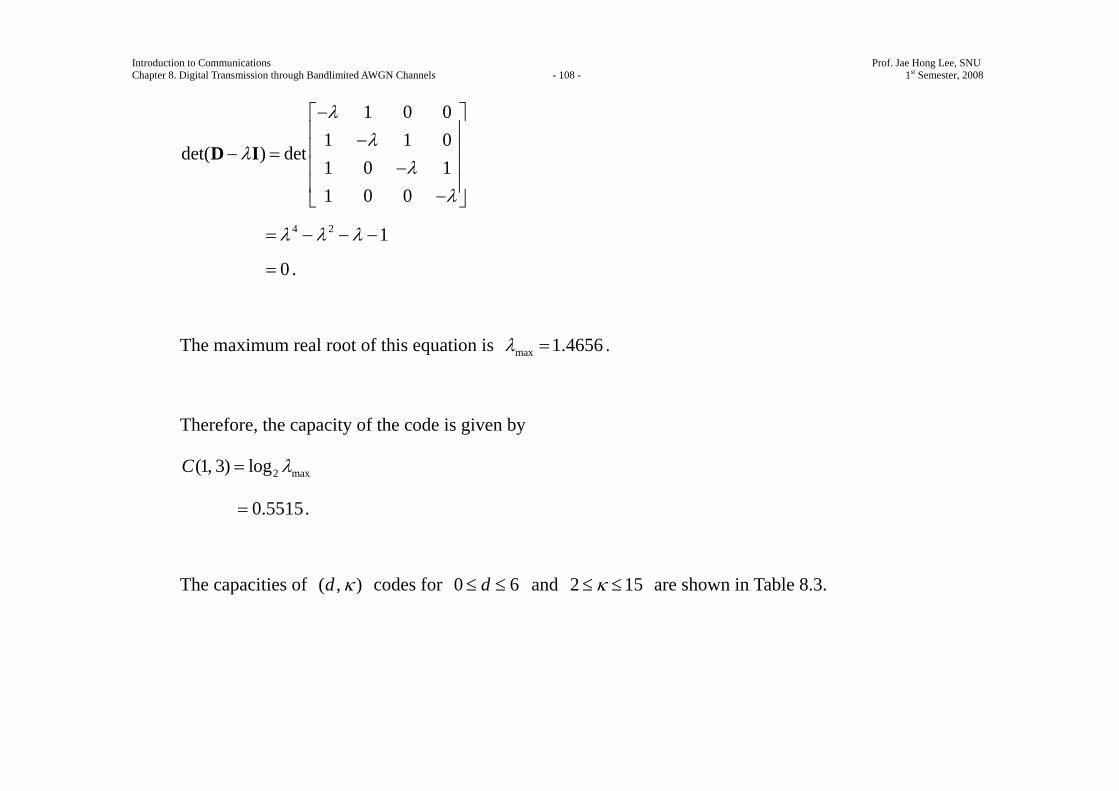
Introduction to Communications Prof. Jae Hong Lee, SNU Chapter 8. Digital Transmission through Bandlimited AWGN Channels - 108 - 1st Semester, 2008
1 0 01 1 0
det( ) det1 0 11 0 0
λλ
λλ
λ
−⎡ ⎤⎢ ⎥−⎢ ⎥− =⎢ ⎥−⎢ ⎥−⎣ ⎦
D I
4 2 1λ λ λ= − − −
0= .
The maximum real root of this equation is max 1.4656λ = .
Therefore, the capacity of the code is given by
2 max(1, 3) logC λ=
0.5515= .
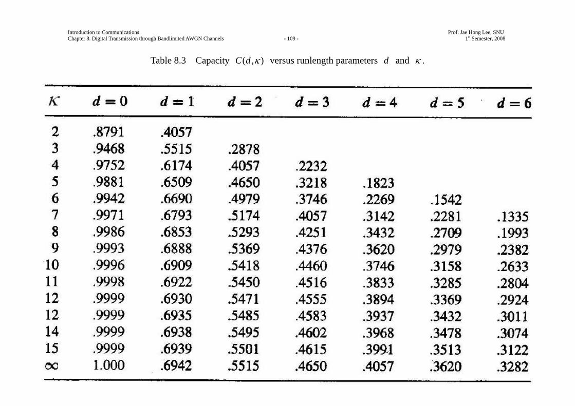
The capacities of ( , )d κ codes for 0 6d≤ ≤ and 2 15κ≤ ≤ are shown in Table 8.3.
Introduction to Communications Prof. Jae Hong Lee, SNU Chapter 8. Digital Transmission through Bandlimited AWGN Channels - 109 - 1st Semester, 2008
Table 8.3 Capacity ( , )C d κ versus runlength parameters d and κ .
Introduction to Communications Prof. Jae Hong Lee, SNU Chapter 8. Digital Transmission through Bandlimited AWGN Channels - 110 - 1st Semester, 2008
In general, ( , )d κ codes can be constructed either as fixed-length codes or variable-length codes.
From Table 8.3, we observe that the capacity 1( , )2
C d κ < for any value of κ when 3d ≥ .
The most commonly used codes for magnetic recording have the minimum number of 0’s between 1’s in a
sequence 2d ≤ .
In a fixed-length code, each bit or block of k bits is encoded into a block of n ( k> ) bits.
To construct a fixed-length code with a given block length n , we may select the subset of the 2n
codewords that satisfy the specified runlength constraints.
From this subset, we eliminate codewords that do not satisfy the runlength constraints when they are
concatenated.
Thus, we obtain a set of codewords that satisfies the runlength constraints which can be used in the mapping
of the input data bit sequences to the encoder.

Introduction to Communications Prof. Jae Hong Lee, SNU Chapter 8. Digital Transmission through Bandlimited AWGN Channels - 111 - 1st Semester, 2008
The encoding and decoding can be performed by using a look-up table.
Ex. 8.5.3
Construct a 0d = , 2κ = code of length 3n = , and determine its efficiency.
Solution
By listing all possible words, we find that the following five codewords which satisfy the (0, 2) constraint:
(010) , (011) , (101) , (110) , (111) .
We may select any four of these five codewords and use them to encode the data sequences of two bits
(0 0, 01,10,11) .
Thus, we have a rate 23c
kRn
= = code that satisfies the (0, 2) constraint.
The capacity of a (0, 2) code is given by

Introduction to Communications Prof. Jae Hong Lee, SNU Chapter 8. Digital Transmission through Bandlimited AWGN Channels - 112 - 1st Semester, 2008
,
21(0, 2) lim log ( )
nC N n
n→∞=
21 log 43
= ⋅
0.8791= ,
so that this code has an efficiency of
efficiency( , )
cRC d κ
=
23
0.8791=
0.76= .
Note that the fixed-length code in this example is not very efficient.
Better (0, 2) codes can be constructed by increasing the block length n .
Introduction to Communications Prof. Jae Hong Lee, SNU Chapter 8. Digital Transmission through Bandlimited AWGN Channels - 113 - 1st Semester, 2008
Ex. 8.5.4
Construct a 1d = , κ = ∞ code of length 5n = .
Solution
From the set of ( 52 = ) 32 possible words, we select the codewords which satisfy the constraint of 1d = .
There are eight such codewords so that we can encode three information bits with each codeword.
The code is given in Table 8.4.
Note that the first bit of each codeword is 0 , whereas the last bit may be either 0 or 1, so that the 1d =
constraint is satisfied when these codewords are concatenated.
This code has a rate 35cR = .
From Table 8.3, the capacity is obtained as (1, ) 0.6942C ∞ = .
Hence, the code efficiency is given by
35efficiency
( , ) 0.6942cR
C d κ= = = 0.864 , which is quite acceptable.
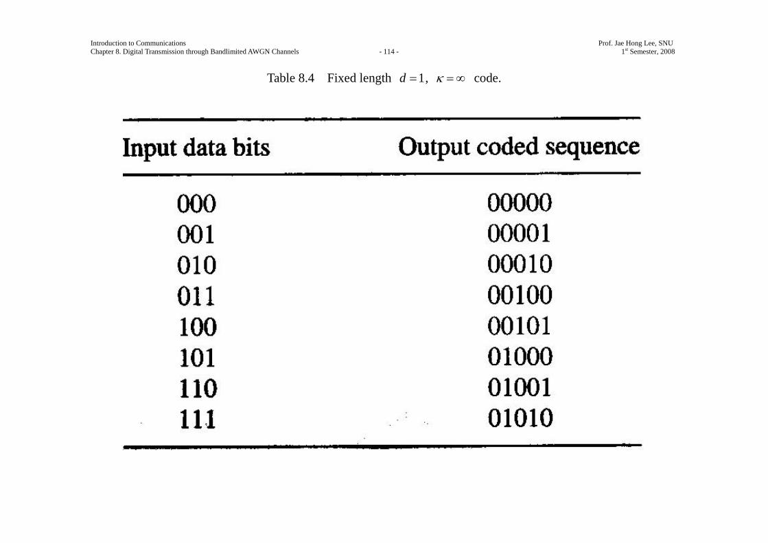
Introduction to Communications Prof. Jae Hong Lee, SNU Chapter 8. Digital Transmission through Bandlimited AWGN Channels - 114 - 1st Semester, 2008
Table 8.4 Fixed length 1d = , κ = ∞ code.
Introduction to Communications Prof. Jae Hong Lee, SNU Chapter 8. Digital Transmission through Bandlimited AWGN Channels - 115 - 1st Semester, 2008
The code construction in the two examples above produces fixed-length ( , )d κ codes that are state
independent which means that fixed-length codewords can be concatenated without violating the ( , )d κ
constraints.
In general, fixed-length, state-independent ( , )d κ codes require large block lengths, except in cases such
as those in the examples above, where d is small.
Simpler (shorter-length) codes are generally possible by allowing for state-dependence and for variable-
length codewords.
Ex. 8.5.5
Construct a simple variable-length 0d = , 2κ = code.
Solution
A very simple uniquely decodable (0, 2) code is as follows:

Introduction to Communications Prof. Jae Hong Lee, SNU Chapter 8. Digital Transmission through Bandlimited AWGN Channels - 116 - 1st Semester, 2008
0 0110 101 1 11.
→→→
This code has a fixed output block length but a variable input block size.
In general, both the input and output blockelngth may be variable. This case is shown in the following
example.
Ex. 8.5.6
Construct a (2, 7) variable blocklength code.
Solution
The (2, 7) code has been widely used by IBM in many of its disk storage systems.
The code is given in Table 8.5.
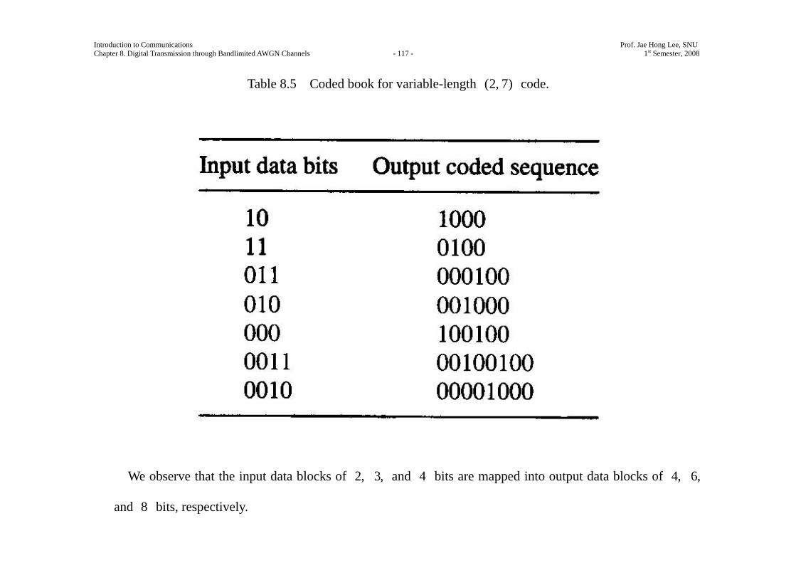
Introduction to Communications Prof. Jae Hong Lee, SNU Chapter 8. Digital Transmission through Bandlimited AWGN Channels - 117 - 1st Semester, 2008
Table 8.5 Coded book for variable-length (2, 7) code.
We observe that the input data blocks of 2, 3, and 4 bits are mapped into output data blocks of 4, 6,
and 8 bits, respectively.
Introduction to Communications Prof. Jae Hong Lee, SNU Chapter 8. Digital Transmission through Bandlimited AWGN Channels - 118 - 1st Semester, 2008
Hence, the code rate is given by 48cR =
12
= .
Since this is the code rate for all codewords, the code is called a fixed-rate code.
This code has an efficiency 0.5 0.9660.5174
= = .
Note that this code satisfies the prefix condition.
Another code that has been widely used in magnetic recording is the rate 12
, ( , ) (1, 3)d κ = code given in
Table 8.6.

Introduction to Communications Prof. Jae Hong Lee, SNU Chapter 8. Digital Transmission through Bandlimited AWGN Channels - 119 - 1st Semester, 2008
Table 8.6 Encoder for (1, 3) Miller code.
We observe that when the information bit is 0 , the first output bit is either 1 , if the previous input bit was
0 , or 0 , if the previous input bit was 1 .
When the information bit is 1 , the encoder output is 0 1 .
Decoding of this code is simple.
The first bit of the two-bit block is redundant and may be discarded.
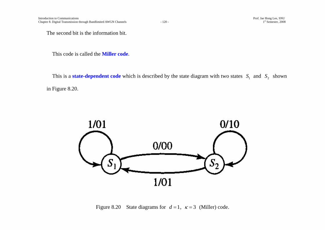
Introduction to Communications Prof. Jae Hong Lee, SNU Chapter 8. Digital Transmission through Bandlimited AWGN Channels - 120 - 1st Semester, 2008
The second bit is the information bit.
This code is called the Miller code.
This is a state-dependent code which is described by the state diagram with two states 1S and 2S shown
in Figure 8.20.
Figure 8.20 State diagrams for 1d = , 3κ = (Miller) code.
Introduction to Communications Prof. Jae Hong Lee, SNU Chapter 8. Digital Transmission through Bandlimited AWGN Channels - 121 - 1st Semester, 2008
When the encoder is a state 1S , an input bit 1 results in the encoder staying in state 1S and outputs 01.
This is represented by 1/ 01.
Trellis Representation of State-Dependent ( , )d κ Codes
Another way to describe codes that have memory is by means of a trellis which is a graph showing the state
transitions as a function of time.
A trellis consists of a set of nodes representing the states which characterize the memory in the code at
different time instants and interconnections between pairs of nodes which indicate the transitions between
successive time instants.
Figure 8.21 shows the trellis for the 1d = , 3κ = Miller code whose state diagram is shown in Figure 8.20.
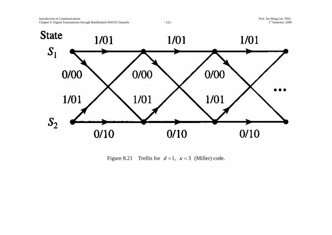
Introduction to Communications Prof. Jae Hong Lee, SNU Chapter 8. Digital Transmission through Bandlimited AWGN Channels - 122 - 1st Semester, 2008
Figure 8.21 Trellis for 1d = , 3κ = (Miller) code.
Introduction to Communications Prof. Jae Hong Lee, SNU Chapter 8. Digital Transmission through Bandlimited AWGN Channels - 123 - 1st Semester, 2008
Mapping of Coded Bits into Signal Waveforms
The output sequence from the ( , )d κ encoder is mapped by the modulator into signal waveforms for
transmission over the channel.
If the binary digit 1 is mapped into a rectangular pulse of amplitude A and the binary digit 0 is mapped
into a rectangular pulse of amplitude A− , the result is a ( , )d κ -coded NRZ modulated signal.
Note that the duration of the rectangular pulses is cc c b
b
RT R TR
= = ,
where bR is the information (bit) rate into the encoder,
bT is the corresponding (uncoded) bit interval, and
cR is the code rate for the ( , )d κ code.
When the ( , )d κ code is a state-independent fixed-length code with code rate ckRn
= , we may consider
each n -bit block as generating one signal waveform of duration cnT .
Introduction to Communications Prof. Jae Hong Lee, SNU Chapter 8. Digital Transmission through Bandlimited AWGN Channels - 124 - 1st Semester, 2008
We have 2kM = signal waveforms, one for each of the 2k possible k -bit data blocks. These coded
waveforms are given by (7.4.22) and (7.4.23).
In this case, there is no dependence between the transmission of successive waveforms.
The modulation signal is no longer memoryless when NRZI is used and, or, the ( , )d κ code is state
dependant.
First, consider the effect of mapping the coded bits into an NRZI signal waveform.
An NRZI modulated signal is itself state dependent.
The signal-amplitude level is changed from its current value ( )A± only when the bit to be transmitted is
1.
Note that the NRZI signal may be viewed as an NRZ signal preceded by another encoding operation, called
precoding, of the binary sequence, as shown in Figure 8.22.
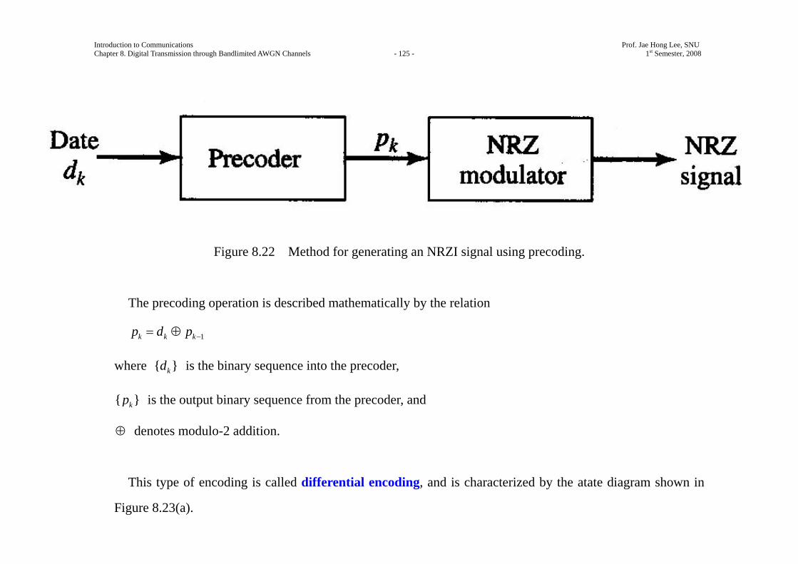
Introduction to Communications Prof. Jae Hong Lee, SNU Chapter 8. Digital Transmission through Bandlimited AWGN Channels - 125 - 1st Semester, 2008
Figure 8.22 Method for generating an NRZI signal using precoding.
The precoding operation is described mathematically by the relation
1k k kp d p −= ⊕
where { }kd is the binary sequence into the precoder,
{ }kp is the output binary sequence from the precoder, and
⊕ denotes modulo-2 addition.
This type of encoding is called differential encoding, and is characterized by the atate diagram shown in
Figure 8.23(a).
Introduction to Communications Prof. Jae Hong Lee, SNU Chapter 8. Digital Transmission through Bandlimited AWGN Channels - 126 - 1st Semester, 2008
Then, the sequence { }kp is transmitted by NRZ.
When 1kp = , the modulator output is a rectangular pulse of amplitude A and when 0kp = , the
modulator output is a rectangular pulse of amplitude A− .
When the signal waveforms are superimposed on the state diagram of Figure 8.23(a), we obtain the
corresponding state diagram shown in Figure 8.23(b).

Introduction to Communications Prof. Jae Hong Lee, SNU Chapter 8. Digital Transmission through Bandlimited AWGN Channels - 127 - 1st Semester, 2008
Figure 8.23 State diagram for NRZI signal.
Introduction to Communications Prof. Jae Hong Lee, SNU Chapter 8. Digital Transmission through Bandlimited AWGN Channels - 128 - 1st Semester, 2008
Differential encoding or precoding as described above introduces memory in the modulated signal.
As in the case of state-dependent ( , )d κ codes, a trellis diagram may be used to show the time dependence
of the modulated signal.
The trellis diagram for the NRZI signal is shown in Figure 8.24.
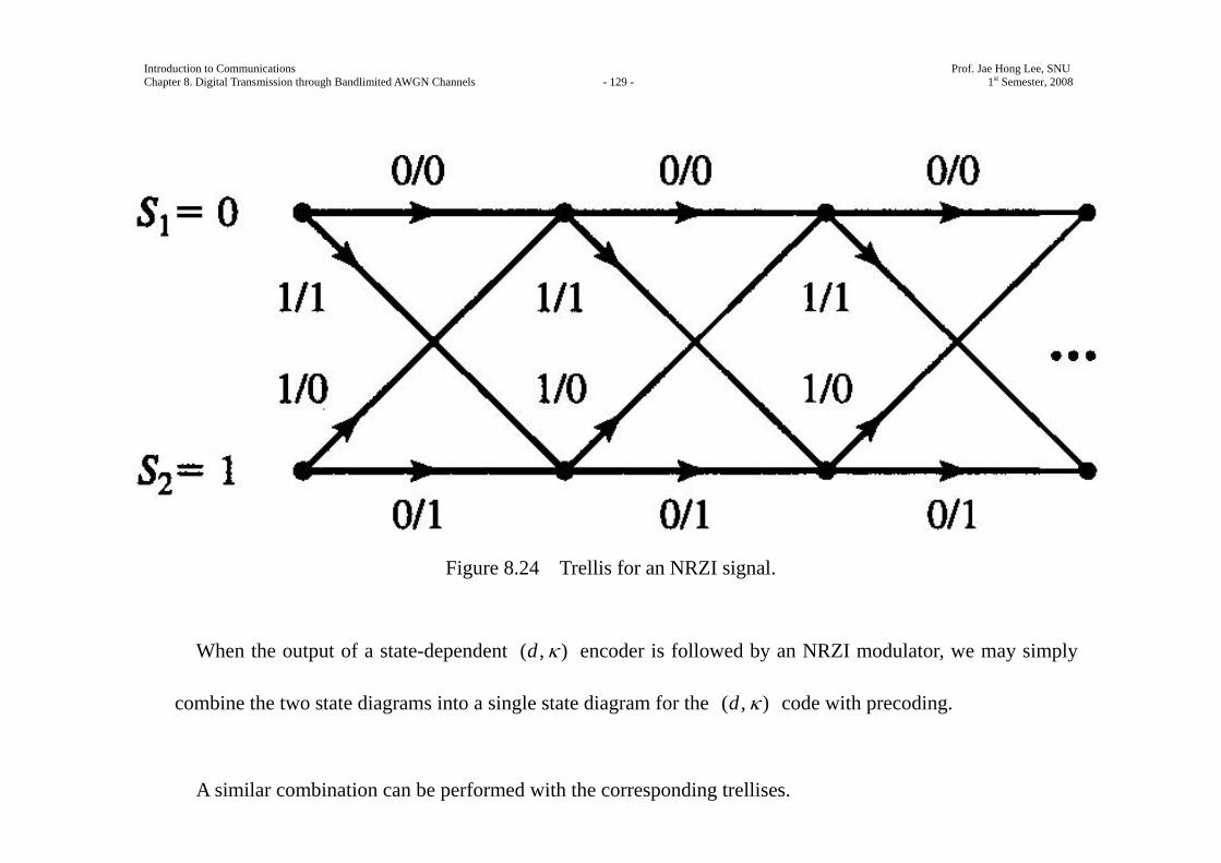
Introduction to Communications Prof. Jae Hong Lee, SNU Chapter 8. Digital Transmission through Bandlimited AWGN Channels - 129 - 1st Semester, 2008
Figure 8.24 Trellis for an NRZI signal.
When the output of a state-dependent ( , )d κ encoder is followed by an NRZI modulator, we may simply
combine the two state diagrams into a single state diagram for the ( , )d κ code with precoding.
A similar combination can be performed with the corresponding trellises.
Introduction to Communications Prof. Jae Hong Lee, SNU Chapter 8. Digital Transmission through Bandlimited AWGN Channels - 130 - 1st Semester, 2008
Ex. 8.5.7
Determine the state diagram of the combined (1, 3) Miller code followed by the precoding inherent in
NRZI modulation.
Solution
Since the (1, 3) Miller code has two states and the precoder has two states, the state diagram for the
combined encoder has four states, which are denoted as 1 1 1 2 2 1 2 2( , ) ( , ), ( , ), ( , ), ( , )M NS S s s s sσ σ σ σ= ,
where 1 2{ , }MS σ σ= represents the two states of the Miller code and
1 2{ , }NS s s= represents the two states of the precoder for NRZI.
For each data input bit into the Miller encoder we obtain two output bits which are then precoded to yield
two precoded output bits.
The resulting state diagram is shown in Figure 8.25, where the first bit denotes the information bit into the
Miller encoder and the next two bits represent the corresponding output of the recoder.
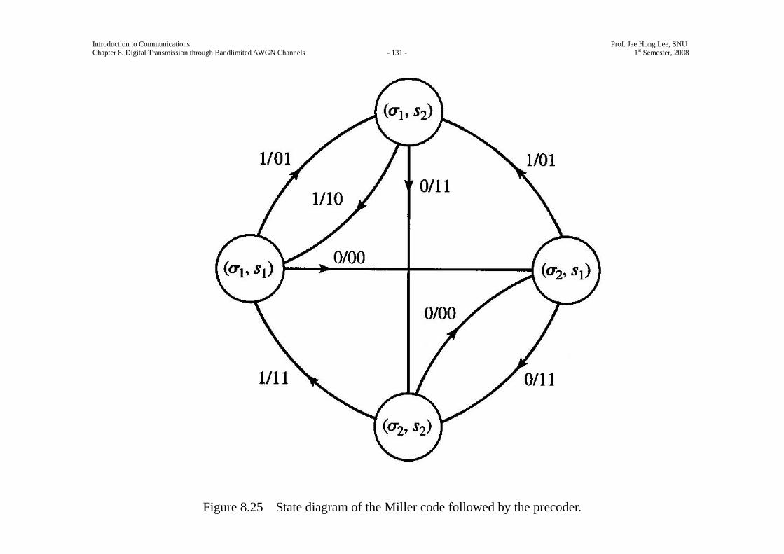
Introduction to Communications Prof. Jae Hong Lee, SNU Chapter 8. Digital Transmission through Bandlimited AWGN Channels - 131 - 1st Semester, 2008
Figure 8.25 State diagram of the Miller code followed by the precoder.
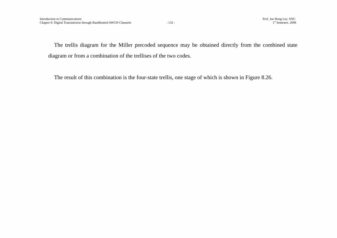
Introduction to Communications Prof. Jae Hong Lee, SNU Chapter 8. Digital Transmission through Bandlimited AWGN Channels - 132 - 1st Semester, 2008
The trellis diagram for the Miller precoded sequence may be obtained directly from the combined state
diagram or from a combination of the trellises of the two codes.
The result of this combination is the four-state trellis, one stage of which is shown in Figure 8.26.
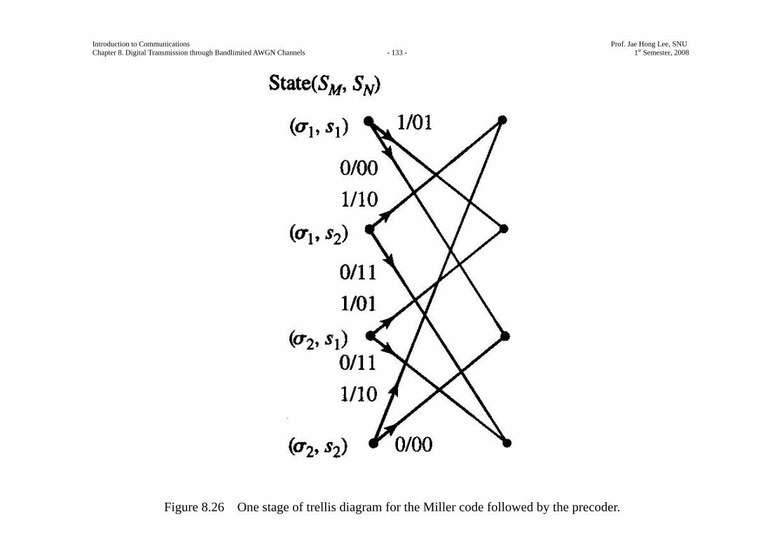
Introduction to Communications Prof. Jae Hong Lee, SNU Chapter 8. Digital Transmission through Bandlimited AWGN Channels - 133 - 1st Semester, 2008
Figure 8.26 One stage of trellis diagram for the Miller code followed by the precoder.
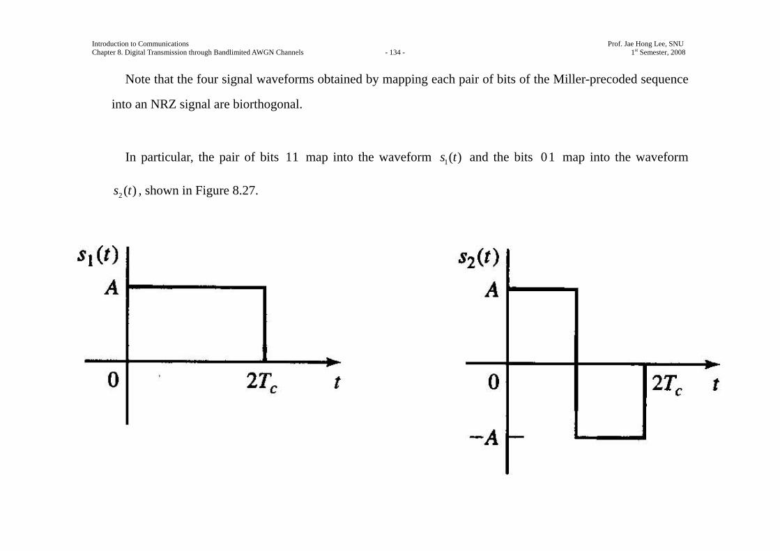
Introduction to Communications Prof. Jae Hong Lee, SNU Chapter 8. Digital Transmission through Bandlimited AWGN Channels - 134 - 1st Semester, 2008
Note that the four signal waveforms obtained by mapping each pair of bits of the Miller-precoded sequence
into an NRZ signal are biorthogonal.
In particular, the pair of bits 11 map into the waveform 1( )s t and the bits 01 map into the waveform
2( )s t , shown in Figure 8.27.

Introduction to Communications Prof. Jae Hong Lee, SNU Chapter 8. Digital Transmission through Bandlimited AWGN Channels - 135 - 1st Semester, 2008
Figure 8.27 Signal waveforms for Miller-precoded pairs of bits.
Then, the encoded bits 0 0 map into 1( )s t− and the bits 10 map into 2 ( )s t− .
Since 1( )s t and 2( )s t are orthogonal, the set of four waveforms constitute a biorthogonal set of 4M =
waveforms.
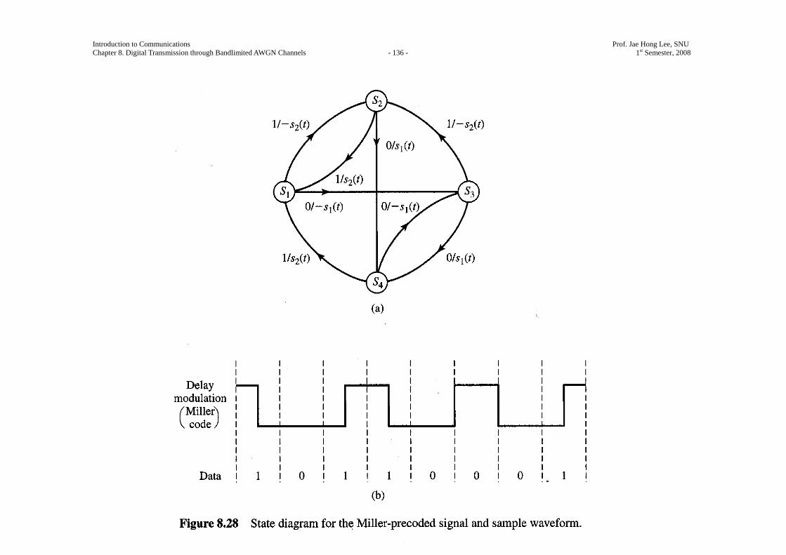
Introduction to Communications Prof. Jae Hong Lee, SNU Chapter 8. Digital Transmission through Bandlimited AWGN Channels - 136 - 1st Semester, 2008
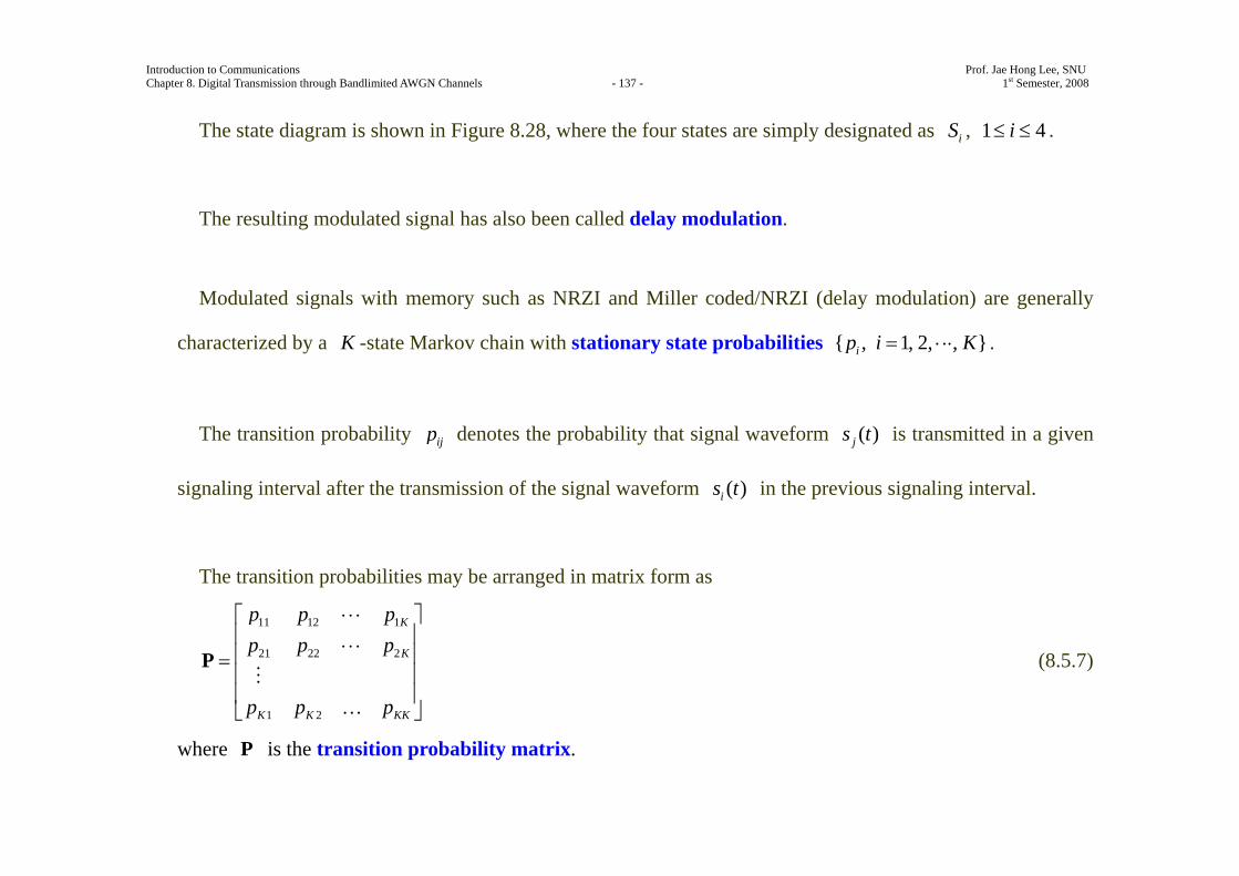
Introduction to Communications Prof. Jae Hong Lee, SNU Chapter 8. Digital Transmission through Bandlimited AWGN Channels - 137 - 1st Semester, 2008
The state diagram is shown in Figure 8.28, where the four states are simply designated as iS , 1 4i≤ ≤ .
The resulting modulated signal has also been called delay modulation.
Modulated signals with memory such as NRZI and Miller coded/NRZI (delay modulation) are generally
characterized by a K -state Markov chain with stationary state probabilities { , 1, 2, , }ip i K= ⋅ ⋅⋅ .
The transition probability ijp denotes the probability that signal waveform ( )js t is transmitted in a given
signaling interval after the transmission of the signal waveform ( )is t in the previous signaling interval.
The transition probabilities may be arranged in matrix form as
11 12 1
21 22 2
1 2
K
K
K K KK
p p pp p p
p p p
⋅ ⋅ ⋅⎡ ⎤⎢ ⎥⋅ ⋅ ⋅⎢ ⎥=⎢ ⎥⎢ ⎥⎣ ⎦
P
…
(8.5.7)
where P is the transition probability matrix.

Introduction to Communications Prof. Jae Hong Lee, SNU Chapter 8. Digital Transmission through Bandlimited AWGN Channels - 138 - 1st Semester, 2008
For the NRZI signal with equal state probabilities 1 212
p p= = and state diagram shown in Figure 8.23, the
transition probability matrix is given by
1 12 21 12 2
⎡ ⎤⎢ ⎥
= ⎢ ⎥⎢ ⎥⎢ ⎥⎣ ⎦
P . (8.5.8)
Similarly, the transition probability matrix for the Miller-coded NRZI modulated signal with equally likely
symbols 1 2 3 41( )4
p p p p= = = = is given by
1 10 02 2
1 10 02 2
1 1 0 02 21 10 02 2
⎡ ⎤⎢ ⎥⎢ ⎥⎢ ⎥⎢ ⎥
= ⎢ ⎥⎢ ⎥⎢ ⎥⎢ ⎥⎢ ⎥⎣ ⎦
P . (8.5.9)
Introduction to Communications Prof. Jae Hong Lee, SNU Chapter 8. Digital Transmission through Bandlimited AWGN Channels - 139 - 1st Semester, 2008
Modulation Code for Compact Disc System
In the design of a modulation code for the compact disc system, several factors had to be considered.
One constraint is that the maximum runlength of zeros must be sufficiently small to allow the system to
synchronize from the readback signal.
To satisfy this constraint, 10κ = was chosen.
A second factor is the frequency content of the modulated signal below 20 kHz.
To avoid interference with these control signals, the modulated information signal must fall above this
frequency range.
The runlength-limited code that was implemented for this purpose is a ( , ) (2,10)d κ = code that results in
a coded that encodes eight information bits into 14 coded bits and is called EFM (eight-to-fourteen
modulation).
Introduction to Communications Prof. Jae Hong Lee, SNU Chapter 8. Digital Transmission through Bandlimited AWGN Channels - 140 - 1st Semester, 2008
Since each audio signal sample is quantized to 16 bits, a 16 -bit sample is divided into two 8 -bit bytes
and encoded.
By enumerating all the 14 -bit codewords, one can show that there are 267 distinct codewords that satisfy
the ( , )d κ constraints.
Of these, 256 codewords are selected to form the code.
However, the ( , )d κ constraints are not satisfied when the codewords are concatenated (merged in a
sequence).
To remedy this problem, three additional bits are added to the 14 , called “merging” bits.
The three merging bits serve two purposes.
First of all, if the d -constraint is not satisfied in concatenation, we choose 0’s for the merging bits.
Introduction to Communications Prof. Jae Hong Lee, SNU Chapter 8. Digital Transmission through Bandlimited AWGN Channels - 141 - 1st Semester, 2008
On the other hand, if the κ -constraint is being violated due to concatenation, we select one of the bits as 1.
Since two bits are sufficient to accomplish these goals, the third merging bit may be viewed as an added
degree of freedom.
This added degree of freedom allows us to use the merging bits to minimize the low-frequency content of
the modulated signal.
Since the merging bits carry no audio signal information, they are discarded in the readback process prior to
decoding.
A measure of the low-frequency content of a digital modulated signal is the running digital sum (RDS),
which is the difference between the total zeros and the total ones in the coded sequence accumulated from the
beginning of the disc.
In addition to satisfying the ( , )d κ constraints, the three merging bits are instrumental in reducing the low-
frequency content below 20 kHz by an additional factor of 10 (in power).
Introduction to Communications Prof. Jae Hong Lee, SNU Chapter 8. Digital Transmission through Bandlimited AWGN Channels - 142 - 1st Semester, 2008
In addition to the coded information bits and merging bits, additional bits are added for control and display
(C & D), synchronization bits, and parity bits.
The data bits, control bits, parity bits, and synchronization bits are arranged in a frame srtructure, consisting
of 588 bits/frame.
The frame structure is shown in Figure 8.29.
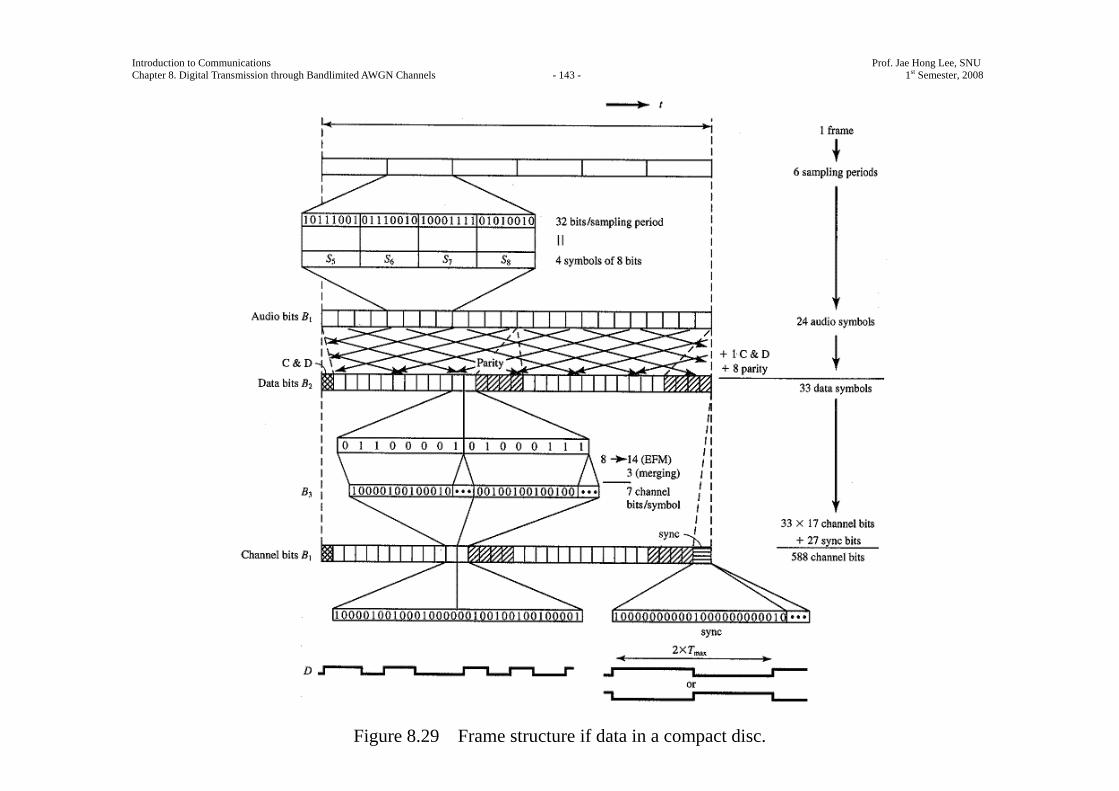
Introduction to Communications Prof. Jae Hong Lee, SNU Chapter 8. Digital Transmission through Bandlimited AWGN Channels - 143 - 1st Semester, 2008
Figure 8.29 Frame structure if data in a compact disc.
Introduction to Communications Prof. Jae Hong Lee, SNU Chapter 8. Digital Transmission through Bandlimited AWGN Channels - 144 - 1st Semester, 2008
8.5.2 The maximum-Likelihood Sequence Detector
When the transmitted signal has memory; i.e., the signals transmitted in successive symbol intervals are
interdependent, the optimum detector bases its decisions on observation of a sequence of received signals over
successive signal intervals.
Consider as an example the NRZI signal described in Section 8.5.1.
Its memory is characterized by the trellis shown in Figure 8.24.
The signal transmitted in each signal interval is binary PAM.
Hence, there are two possible transmitted signals corresponding to the signal points 1 2 bs s ε= − = , where
bε is the energy/bit.
As shown in Section 7.5, the output of the matched-filter or correlation-type demodulator for binary PAM in
the k th signal interval is given by

Introduction to Communications Prof. Jae Hong Lee, SNU Chapter 8. Digital Transmission through Bandlimited AWGN Channels - 145 - 1st Semester, 2008
k b kr nε= ± + (8.5.10)
where kn is a zero-mean Gaussian random variable with variance 2 0
2nNσ = .
Consequently, the conditional PDFs for the two possible transmitted signals are given by 2
2( )
21
1( | )2
k b
n
r
kn
f r s eε
σ
πσ
−−
=
2
2( )
22
1( | )2
k b
n
r
kn
f r s eε
σ
πσ
+−
= . (8.5.11)
Now, suppose we observe the sequence of matched-filter outputs 1 2, , , Kr r r .
Since the channel noise is assumed to be white and Gaussian, and ( ),t iTψ − ( )t jTψ − for i j≠ are
orthogonal, it follows that ( ) 0k jE n n = , k j≠ .
Hence, the noise sequence 1 2, , , kn n n is also white.
Introduction to Communications Prof. Jae Hong Lee, SNU Chapter 8. Digital Transmission through Bandlimited AWGN Channels - 146 - 1st Semester, 2008
Consequently, for any given transmitted sequence ( )ms , the joint PDF of 1 2, , , Kr r r is expressed as a
product of k marginal PDFs; i.e.,
( ) ( )1 2
1
( , , , | ) ( | )K
mK k k
k
p r r r p r s=
=∏ms
( ) 2
2( )
2
1
12
mk k
n
r sK
k n
e σ
πσ
−
=
=∏
( ) 2
21
1 ( )exp22
K mKk k
k nn
r sσπσ =
⎛ ⎞ ⎡ ⎤−= −⎜ ⎟ ⎢ ⎥
⎣ ⎦⎝ ⎠∑ (8.5.12)
where either k bs ε= or k bs ε= − .
Then, given the received sequence 1 2, , , Kr r r at the output of the matched-filter or correlation-type
demodulator, the detector determines the sequence ( ) ( ) ( ) ( )1 2{ , , , }m m m
Ks s s=ms that maximizes the conditional
PDF ( )1 2( , , | )m
Kp r r r s .
Such a detector is called the maximum-likelihood ( )ML sequence detector.
Introduction to Communications Prof. Jae Hong Lee, SNU Chapter 8. Digital Transmission through Bandlimited AWGN Channels - 147 - 1st Semester, 2008
Taking the logarithm of (8.5.12) and neglecting the terms that are independent of 1 2( , , )Kr r r , we find that
an equivalent ML sequence detector select the sequence ( )ms that minimizes the Euclidean distance metric:
( ) ( ) 2
1
( , ) ( )K
m mk k
k
D r s=
= −∑r s . (8.5.13)
In searching through the trellis for the sequence that minimizes the Euclidean distance ( )( , )mD r s , it may
appear that we must compute the distance ( )( , )mD r s for every possible path (sequence).
For the NRZI example given above, which employs binary modulation, the total number of paths is 2K ,
where K is the number of outputs obtained from the demodulator.
We may reduce the number of sequences in the trellis search by using the Viterbi algorithm to eliminate
sequences as new data is received from the demodulator.
The Viterbi algorithm is a sequential trellis search algorithm for performing ML sequence detection to be
described in detail in Chapter 9 as a decoding algorithm for channel-coded systems.

Introduction to Communications Prof. Jae Hong Lee, SNU Chapter 8. Digital Transmission through Bandlimited AWGN Channels - 148 - 1st Semester, 2008
We describe it below in the context of the NRZI signal.
Assume that the search process begins initially at state 1S .
The corresponding trellis is shown in Figure 8.30.
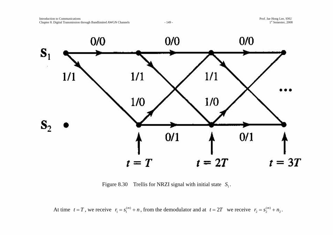
Introduction to Communications Prof. Jae Hong Lee, SNU Chapter 8. Digital Transmission through Bandlimited AWGN Channels - 149 - 1st Semester, 2008
Figure 8.30 Trellis for NRZI signal with initial state 1S .
At time t T= , we receive ( )1 1
mr s n= + , from the demodulator and at 2t T= we receive ( )2 2 2
mr s n= + .
Introduction to Communications Prof. Jae Hong Lee, SNU Chapter 8. Digital Transmission through Bandlimited AWGN Channels - 150 - 1st Semester, 2008
Since the signal memory is one bit, which we denote as 1L = , we observe that the trellis reaches its regular
(steady-state) form after the first transition.
Thus, upon receipt of 2r at 2t T= (and thereafter), we observe that there are two signal paths entering
each of the two nodes and two signal paths leaving each node.
The two paths entering node 1S at 2t T= correspond to the information bits (0, 0) and (1,1) or,
equivalently, to the signal points ( , )b bε ε− − and ( , )b bε ε− , respectively.
The two paths entering node 2S at 2t T= correspond to the information bits (0,1) and (1, 0) or,
equivalenty, to the signal points ( , )b bε ε− and ( , )b bε ε , respectively.
For the two paths entering node 1S , we compute the two Euclidean distance metrics
2 22 1 2(0, 0) ( ) ( )b br rμ ε ε= + + +
2 22 1 2(1,1) ( ) ( )b br rμ ε ε= − + + (8.5.14)
Introduction to Communications Prof. Jae Hong Lee, SNU Chapter 8. Digital Transmission through Bandlimited AWGN Channels - 151 - 1st Semester, 2008
by using the outputs 1r and 2r from the demodulator.
The Viterbi algorithm compares these two metrics and discards the path having the larger (greater distanc)
metric.
The other path with the lower metric is saved and is called the survivor at 2t T= .
The elimination of one of the two paths may be done without compromising the optimality of the trellis
search, because any extension of the path with the larger distance beyond 2t T= will always have a larger
metric than the survivor that is extended along the same path beyond 2t T= .
Similarly, for the two paths entering node 2S at 2t T= , we compute the two Euclidean distance metrics
2 22 1 2(0,1) ( ) ( )b br rμ ε ε= + + −
2 22 1 2(1, 0) ( ) ( )b br rμ ε ε= − + − (8.5.15)
by using the outputs 1r and 2r from the demodulator.
Introduction to Communications Prof. Jae Hong Lee, SNU Chapter 8. Digital Transmission through Bandlimited AWGN Channels - 152 - 1st Semester, 2008
The two metrics are compared and the signal path with the larger metric is eliminated.
Thus, at 2t T= , we are left with two survivor paths, one at node 1S and the other at node 2S , and their
corresponding metrics.
The signal paths at nodes 1S and 2S are then extended along the two survivor paths.
Upon receipt of 3r at 3t T= , we compute the metrics of the two paths entering state 1S . Suppose the
survivors at 2t T= are the paths (0, 0) at 1S and (0,1) at 2S .
Then, the two metrics for the paths entering 1S at 3t T= are given by
23 2 3(0, 0, 0) (0, 0) ( )brμ μ ε= + +
23 2 3(0,1,1) (0,1) ( )brμ μ ε= + + .
(8.5.16) These two metrics are compared and the path with the larger (distance) metric is eliminated.
Similarly, the metrics for the two paths entering 2S at 3t T= are given by
Introduction to Communications Prof. Jae Hong Lee, SNU Chapter 8. Digital Transmission through Bandlimited AWGN Channels - 153 - 1st Semester, 2008
23 2 3(0,0,1) (0, 0) ( )brμ μ ε= + −
23 2 3(0,1, 0) (0,1) ( )brμ μ ε= + − (8.5.17)
These two metrics are compared and the path with the larger (distance) metric is eliminated.
This process is continued as each new signal sample is received from the demodulator.
Thus, the Viterbi algorithm computes two metrics for the two signal paths entering a node at each stage of
the trellis search and eliminates one of the next stage.
Therefore, the number of paths searched in the trellis is reduced by a factor of two at each stage.
It is relatively easy to generalize the trellis shown in Figure 8.26.
The memory of the signal is 1L = .
From the description of the Viterbi algorithm given above, it is unclear as to how decisions are made on the
Introduction to Communications Prof. Jae Hong Lee, SNU Chapter 8. Digital Transmission through Bandlimited AWGN Channels - 154 - 1st Semester, 2008
individual detected information symbols given the surviving sequences.
If we have advanced to some stage, say K , where K >> L , in the trellis and we compare the surviving
sequences, we will find that, with probability approaching one, all surviving sequences will be identical in bit
(or symbol) positions 5K L− and less.
In a practical implementation of the Viterbi algorithm, decisions on each information bit (or symbol) are
forced after a delay of 5L bits (or symbol) and, hence, the surviving sequences are truncated to the 5L most
recent bits (or symbol).
Thus, a variable delay in bit or symbol detection is avoided. The loss in performance resulting from the
suboptimum detection procedure is negligible if the delay is at least 5L .
Ex. 8.5.8
Describe the decision rule for detecting the data sequence in an NRZI signal with a Viterbi algorithm having
a delay of 5L bits.
Solution
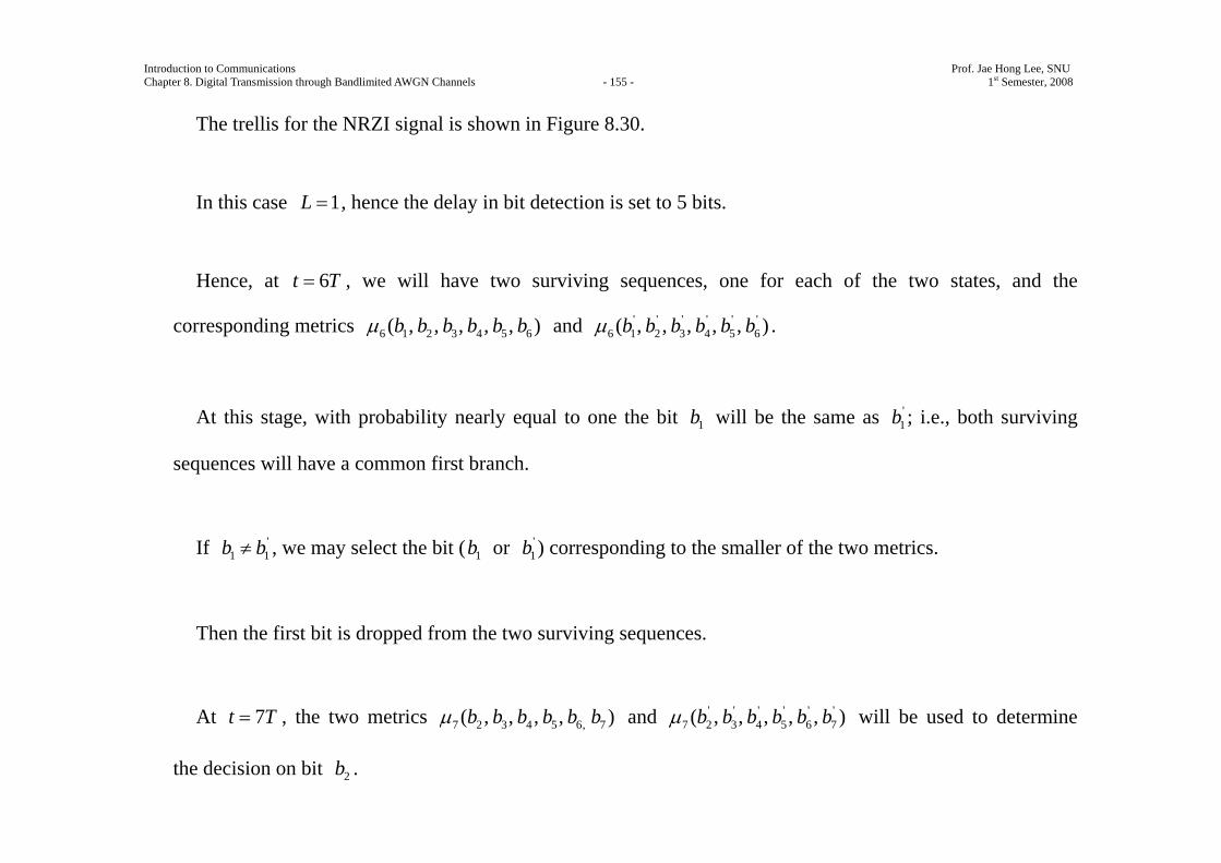
Introduction to Communications Prof. Jae Hong Lee, SNU Chapter 8. Digital Transmission through Bandlimited AWGN Channels - 155 - 1st Semester, 2008
The trellis for the NRZI signal is shown in Figure 8.30.
In this case 1L = , hence the delay in bit detection is set to 5 bits.
Hence, at 6t T= , we will have two surviving sequences, one for each of the two states, and the
corresponding metrics 6 1 2 3 4 5 6( , , , , , )b b b b b bμ and ' ' ' ' ' '6 1 2 3 4 5 6( , , , , , )b b b b b bμ .
At this stage, with probability nearly equal to one the bit 1b will be the same as '1b ; i.e., both surviving
sequences will have a common first branch.
If '1 1b b≠ , we may select the bit ( 1b or '
1b ) corresponding to the smaller of the two metrics.
Then the first bit is dropped from the two surviving sequences.
At 7t T= , the two metrics 7 2 3 4 5 6, 7( , , , , )b b b b b bμ and ' ' ' ' ' '7 2 3 4 5 6 7( , , , , , )b b b b b bμ will be used to determine
the decision on bit 2b .
Introduction to Communications Prof. Jae Hong Lee, SNU Chapter 8. Digital Transmission through Bandlimited AWGN Channels - 156 - 1st Semester, 2008
This process continues at each stage of the search through the trellis for the minimum distance sequence.
Thus the detection delay is fixed at 5 bits.
8.5.3 Maximum-Likelihood Sequence Detection of Partial Response Signals
Partial response waveforms are signal waveforms with memory.
This memory is conveniently represented by a trellis.
For example, the trellis for the duobinary partial response signal for binary data transmission is shown in
Figure 8.31.
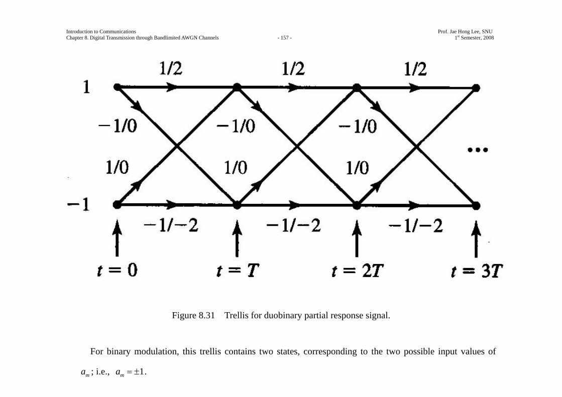
Introduction to Communications Prof. Jae Hong Lee, SNU Chapter 8. Digital Transmission through Bandlimited AWGN Channels - 157 - 1st Semester, 2008
Figure 8.31 Trellis for duobinary partial response signal.
For binary modulation, this trellis contains two states, corresponding to the two possible input values of
ma ; i.e., 1ma = ± .
Introduction to Communications Prof. Jae Hong Lee, SNU Chapter 8. Digital Transmission through Bandlimited AWGN Channels - 158 - 1st Semester, 2008
Each branch in the trellis is labled by two numbers.
The first number on the left is the new data bit; i.e., 1 1ma + = ± .
This number determines the transition to the new state.
The number on the right is the received signal level.
The duobinary signal has a memory of length 1L = .
Hence, for binary modulation the trellis has 2LtS = states.
In general, for M -ary modulation, the number of trellis states is LM .
The optimum ML sequence detector selects the most probable path through the trellis upon observing the
received data sequence { }my at the sampling instants t mT= , 1, 2,m = .
Introduction to Communications Prof. Jae Hong Lee, SNU Chapter 8. Digital Transmission through Bandlimited AWGN Channels - 159 - 1st Semester, 2008
In general, each node in the trellis will have M incoming paths and M corresponding metrics.
One out of the M incoming paths is selected as the most probable, based on the values of the metrics and
the other 1M − paths and their metrics, are discarded.
The surviving path at each node is then extended to M new paths, one for each of the M possible input
symbols, and the search process continues.
This is basically the Viterbi algorithm for performing the trellis search.
For the class of partial response signals, the received sequence { ,1 }my m N≤ ≤ is generally described
statistically by the joint PDF ( | )N Nf y a ,
where 1 2( , , , )tN Ny y y=y , 1 2,( , , )t
N Na a a=a and N L> .
Introduction to Communications Prof. Jae Hong Lee, SNU Chapter 8. Digital Transmission through Bandlimited AWGN Channels - 160 - 1st Semester, 2008
When the additive noise is zero-mean Gaussian, ( | )N Nf y a is a multivariate Gaussian PDF; i.e.,
11( ) ( )2
2 2
1( | )(2 ) | det( ) |
tN N N N
N N N Nf eπ
−− − −=
y b C y by a
C (8.5.18)
where 1 2( , , , )tN Nb b b=b is the mean of the vector Ny and
C is the N N× covariance matrix of Ny .
Then, the maximum-likelihood sequence detector selects the sequence through the trellis that maximizes the
PDF ( | )N Nf y a .
The computations for finding the most probable sequence through the trellis is simplified by taking the
natural logarithms of ( | )N Nf y a .
Thus,
11 1ln ( | ) ln(2 ) ln | det( ) | ( ) ( )2 2 2
tN N N N N N
Nf π −= − − − − −y a C y b C y b (8.5.19)
Introduction to Communications Prof. Jae Hong Lee, SNU Chapter 8. Digital Transmission through Bandlimited AWGN Channels - 161 - 1st Semester, 2008
Given the received sequence { }my , the data sequence { }ma that maximizes ln ( | )N Nf y a is identical to
the sequence { }ma that minimizes 1( ) ( )tN N N N
−− −y b C y b ; i.e.,
1ˆ arg min( ) ( )tN N N N N
−= − −Naa y b C y b .
The search through the trellis for the minimum distance path may be performed sequentially by use of the
Viterbi algorithm.
Let us consider the duobinary signal waveform with binary modulation and suppose that we begin at the
initial state with 0 1a = .
Then upon receiving 1 1 0 1y a a v= + + at time t T= and 2 2 1 2y a a v= + + at time 2t T= ,
we have four candidate paths, corresponding to 1 2( , ) (1, 1),a a = ( 1,1),− (1, 1)− , and ( 1, 1)− − .
The first two candidate paths merge at state 1 at 2t T= .
Introduction to Communications Prof. Jae Hong Lee, SNU Chapter 8. Digital Transmission through Bandlimited AWGN Channels - 162 - 1st Semester, 2008
For the two paths merging at state 1, we compute the metrics 2(1,1)μ and 2( 1,1)μ − and select the more
probable path.
A similar computation is performed at state 1− for the two sequences (1, 1)− and ( 1, 1)− − .
Thus, one of the two sequences at each node is saved and the other is discarded.
The trellis search continues upon receipt of the signal samply 3y at time 3t T= , by extending the two
surviving paths from time 2t T= .
The metric computations are complicated by the correlation of the noise samples at the output of the
matched filter for the partial response signal.
For example, in the case of the duobinary signal waveform, the correlation of the noise sequence { }mv is
over two successive signal samples.
Hence, mv and m kv + are correlated for 1k = and uncorrelated for 1k > .
Introduction to Communications Prof. Jae Hong Lee, SNU Chapter 8. Digital Transmission through Bandlimited AWGN Channels - 163 - 1st Semester, 2008
In general, a partial response signal waveform with memory L will result in a correlated noise sequence at
the output of the matched filter, which satisfies the condition [ ] 0m m kE v v + = for k L> .
Ungweboeck (1974) described a sequential trellis search (Viterbi) algorithm for correlated noise (see
Problem 8.26).
Some simplification in the metric computations results if we ignore the noise correlation by assuming that
( ) 0m m kE v v + = for 0k > .
Then, by assumption the covariance matrix 2vσ=C I where 2 2
v [ ]mE vσ = and I in the N N× identity
matrix.
In this case, (8.5.20) simplifies to
ˆ arg min[( ) ( )]N
tN N N N N= − −aa y b y b
2
1 0arg min
N
N L
m k m km k
y x a −= =
⎡ ⎤⎛ ⎞= −⎢ ⎥⎜ ⎟
⎝ ⎠⎢ ⎥⎣ ⎦∑ ∑a (8.5.21)
Introduction to Communications Prof. Jae Hong Lee, SNU Chapter 8. Digital Transmission through Bandlimited AWGN Channels - 164 - 1st Semester, 2008
where
0
L
m k m kk
b x a −=
=∑ (8.5.22)
and ( )kx x kT= are the sampled values of the partial response signal waveform.
In this case, the metric computations at each node of the trellis have the form 2
1 10
( ) ( )L
m m m m m k m kk
y x aμ μ − − −=
⎛ ⎞= + −⎜ ⎟
⎝ ⎠∑a a (8.5.23)
where ( )m mμ a are the metrics at time t mT= , 1 1( )m mμ − −a are the metrics at time ( 1)t m T= − and the
second term on the right-hand side of (8.5.23) are the new increments to the metrics based on the new received
samples my .
ML sequence detection introduces a variable delay in detecting each transmitted information symbol.
In practice, the variable delay in avoided by truncating the surviving sequences to tN most recent symbols,
where 5tN L>> , thus achieving a fixed delay.

Introduction to Communications Prof. Jae Hong Lee, SNU Chapter 8. Digital Transmission through Bandlimited AWGN Channels - 165 - 1st Semester, 2008
In case the LM surviving sequences at time t mT= disagree on the symbol tm Na − , the symbol in the
most probable surviving sequence may be chosen.
The loss in performance resulting from this truncation is negligible if 5tN L> .
Ex. 8.5.9
For the duobinary partial response signal, express the metric computations performed at 2t T= and 3t T= ,
based on the received signal samples m m my b v= + for 1,2,3,m = , where the noise correlation is ignored.
Solution
The metrics are generally given by (8.5.23).
Upon receipt of 1y and 2y and with 0 1a = , the metrics for the two paths merging at state 1 are given by
2 22 1 2(1,1) ( 2) ( 2)y yμ = − + −
2 22 1 2( 1,1) y yμ − = + .
Introduction to Communications Prof. Jae Hong Lee, SNU Chapter 8. Digital Transmission through Bandlimited AWGN Channels - 166 - 1st Semester, 2008
If 2 2(1,1) ( 1,1)μ μ< − we select the path (1, 1) as the more probable and discard ( 1,1)− .
Otherwise, we select the path ( 1,1)− and discard the path (1, 1).
The path with the smaller metric is called the survivor and the sequence 1 2( , )a a and the corresponding
metric are saved.
A similar computation is performed at state 1− for the sequences 2y and ( 1, 1)− − .
Then, we have
2 22 1 2(1, 1) ( 2)y yμ − = − +
2 22 1 2( 1, 1) ( 2)y yμ − − = + + .
We compare the metrics 2 (1, 1)μ − and 2 ( 1, 1)μ − − and select the sequence with the smaller metric.
Upon receipt of 3y at 3t T= , we consider the extensions of the survivor paths.
Introduction to Communications Prof. Jae Hong Lee, SNU Chapter 8. Digital Transmission through Bandlimited AWGN Channels - 167 - 1st Semester, 2008
Suppose that the two survivor paths are 1 2( , ) (1,1)a a = and 1 2( , ) (1, 1)a a = − .
Then, at state 1 (at 3t T= ) we have the two merging paths 1 2 3( , , ) (1,1,1)a a a = and (1, 1,1)− .
Their corresponding metrics are given by
23 2 3(1,1,1) (1,1) ( 2)yμ μ= + −
23 2 3(1, 1,1) (1, 1) yμ μ− = − + .
We compare the metrics for these two merging paths and select the path with the smaller metrics as the
survivor.
Similarly, at state 1− (at 3t T= ), we have the two merging paths (1,1, 1)− and (1, 1, 1)− − , and their
corresponding metrics
23 2 3(1,1, 1) (1,1) yμ μ− = +
22 2 3(1, 1, 1) (1, 1) ( 2)yμ μ− − = − + + .
Introduction to Communications Prof. Jae Hong Lee, SNU Chapter 8. Digital Transmission through Bandlimited AWGN Channels - 168 - 1st Semester, 2008
We select the path with the smaller metrics as the survivor at state 1− .
This process continues upon receipt of additional data at t kT= , 4, 5,k = .
Error Probability of the Maximum-Likelihood Sequence Detector
In general, the computation of the exact probability of error is extremely difficult.
Instead, we shall determine an approximation to the probability of error, which is based on comparing the
metrics of two paths which merge at a node and which are separated by the smallest Euclidean distance of all
other paths.
Let us consider the trellis for the duobinary partial response signal shown in Figure 8.31.
Assume that we start in state 1 at 0t = and that the first two transmitted symbols are 1 1a = and 2 1a = .
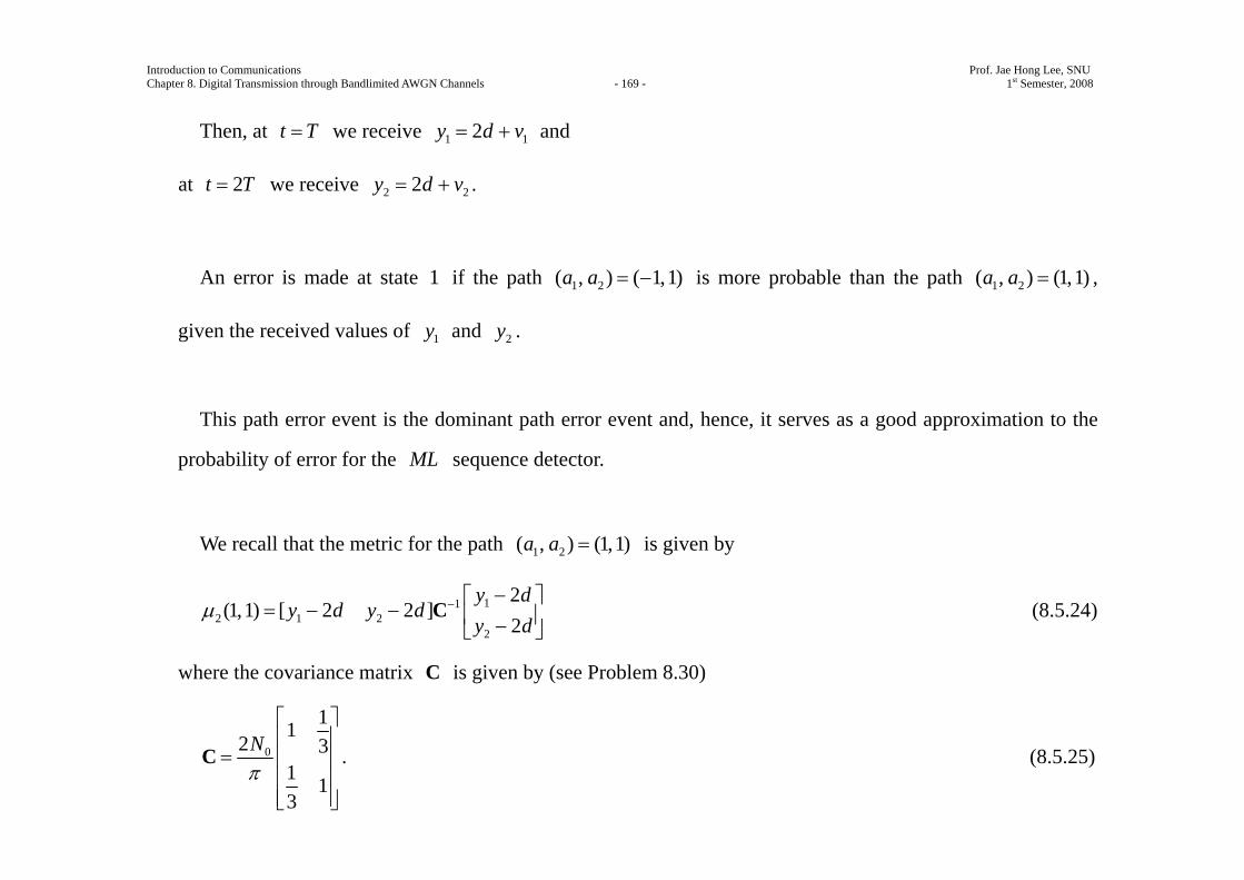
Introduction to Communications Prof. Jae Hong Lee, SNU Chapter 8. Digital Transmission through Bandlimited AWGN Channels - 169 - 1st Semester, 2008
Then, at t T= we receive 1 12y d v= + and
at 2t T= we receive 2 22y d v= + .
An error is made at state 1 if the path 1 2( , ) ( 1,1)a a = − is more probable than the path 1 2( , ) (1,1)a a = ,
given the received values of 1y and 2y .
This path error event is the dominant path error event and, hence, it serves as a good approximation to the
probability of error for the ML sequence detector.
We recall that the metric for the path 1 2( , ) (1,1)a a = is given by
112 1 2
2
2(1,1) [ 2 2 ]
2y d
y d y dy d
μ − −⎡ ⎤= − − ⎢ ⎥−⎣ ⎦
C (8.5.24)
where the covariance matrix C is given by (see Problem 8.30)
0
112 3
1 13
Nπ
⎡ ⎤⎢ ⎥
= ⎢ ⎥⎢ ⎥⎢ ⎥⎣ ⎦
C . (8.5.25)
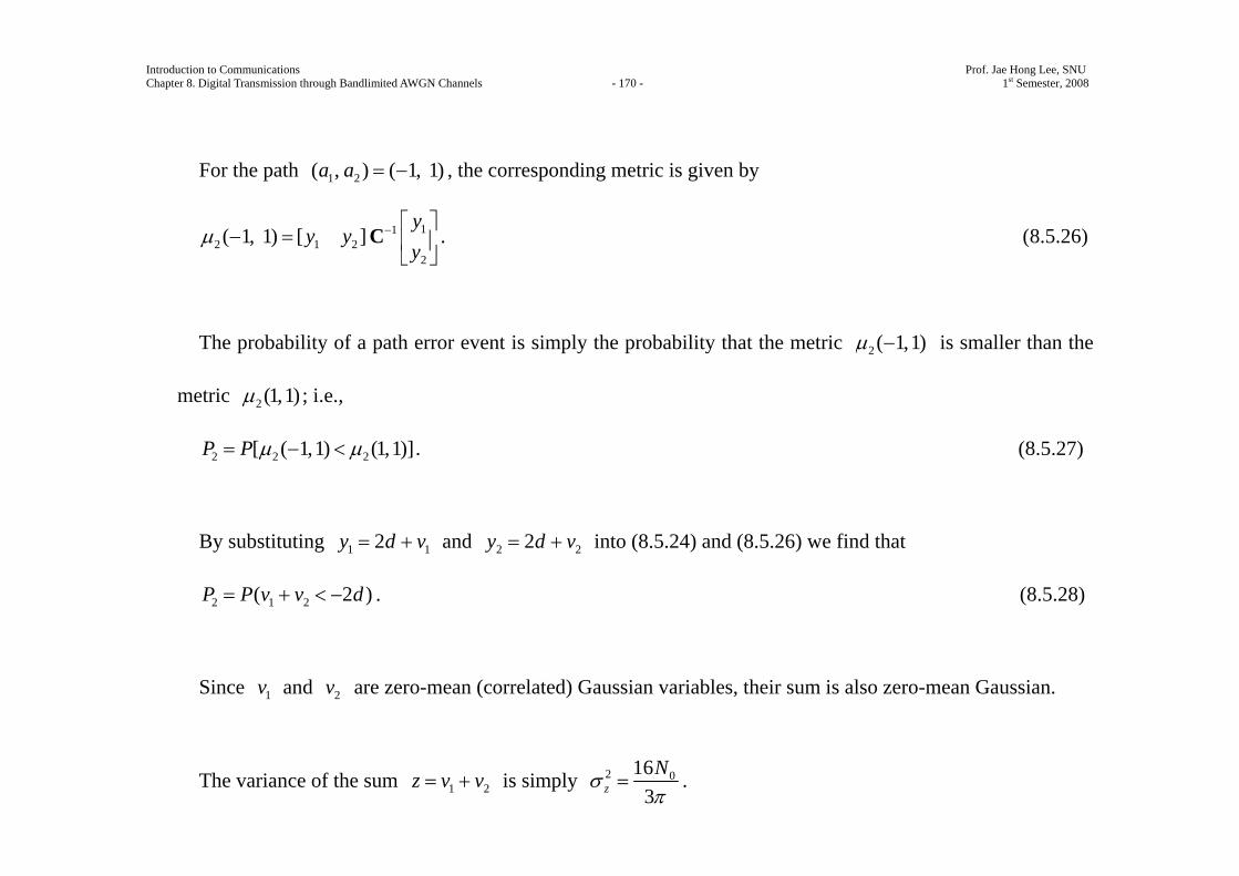
Introduction to Communications Prof. Jae Hong Lee, SNU Chapter 8. Digital Transmission through Bandlimited AWGN Channels - 170 - 1st Semester, 2008
For the path 1 2( , ) ( 1, 1)a a = − , the corresponding metric is given by
112 1 2
2
( 1, 1) [ ]y
y yy
μ − ⎡ ⎤− = ⎢ ⎥
⎣ ⎦C . (8.5.26)
The probability of a path error event is simply the probability that the metric 2 ( 1,1)μ − is smaller than the
metric 2 (1,1)μ ; i.e.,
2 2 2[ ( 1,1) (1,1)]P P μ μ= − < . (8.5.27)
By substituting 1 12y d v= + and 2 22y d v= + into (8.5.24) and (8.5.26) we find that
2 1 2( 2 )P P v v d= + < − . (8.5.28)
Since 1v and 2v are zero-mean (correlated) Gaussian variables, their sum is also zero-mean Gaussian.
The variance of the sum 1 2z v v= + is simply 2 0163zNσπ
= .
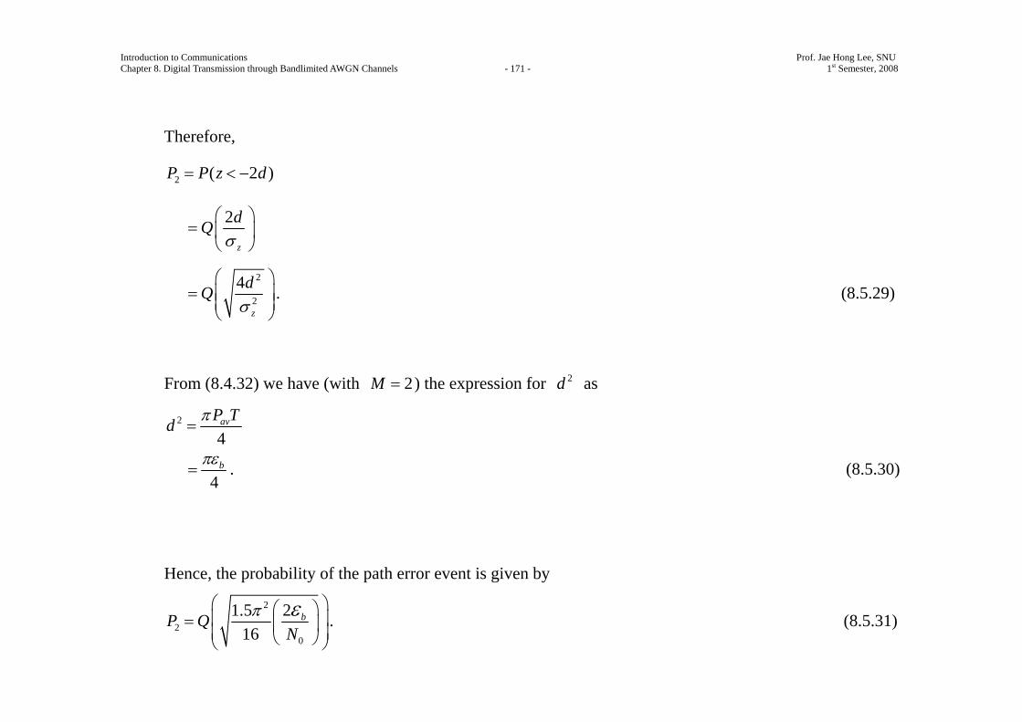
Introduction to Communications Prof. Jae Hong Lee, SNU Chapter 8. Digital Transmission through Bandlimited AWGN Channels - 171 - 1st Semester, 2008
Therefore,
2 ( 2 )P P z d= < −
2
z
dQσ
⎛ ⎞= ⎜ ⎟
⎝ ⎠
2
2
4
z
dQσ
⎛ ⎞= ⎜ ⎟⎜ ⎟
⎝ ⎠. (8.5.29)
From (8.4.32) we have (with 2M = ) the expression for 2d as
2
4avP Td π
=
4bπε
= . (8.5.30)
Hence, the probability of the path error event is given by
2
20
1.5 216
bP QN
π ε⎛ ⎞⎛ ⎞⎜ ⎟= ⎜ ⎟⎜ ⎟⎝ ⎠⎝ ⎠
. (8.5.31)
Introduction to Communications Prof. Jae Hong Lee, SNU Chapter 8. Digital Transmission through Bandlimited AWGN Channels - 172 - 1st Semester, 2008
First, we note that this path error event results in one bit-error in the sequence of two bits.
Hence, the bit-error probability is 2
2P .
Second, there is a reduction in SNR of 21.510 log 0.34 dB
16π
= − relative to the case of no intersymbol
interference.
This small SNR degradation is apparently the penalty incurred in exchange for the bandwidth efficiency of
the partial response signal.
Finally, we observe that the ML sequence detector has gained back 1.76 dB of the 2.1 dB degradation
inherent in the symbol-by-symbol detector.
Introduction to Communications Prof. Jae Hong Lee, SNU Chapter 8. Digital Transmission through Bandlimited AWGN Channels - 173 - 1st Semester, 2008
8.5.4 Power Spectral Density of Digital Signals with Memory
In Section 8.5.1, we demonstrated that state-dependent modulation codes resulted in modulated signals with
memory.
Such signals were described by Markov chains which are basically graphs that include the possible “states”
of the modulator with corresponding state probabilities { }ip , and state transitions with corresponding state
transition probabilities { }ijp .
The power-spectral density of digitally modulated signals that are characterized by Markov chins may be
derived by following the basic procedure given in Section 8.2.
Thus, we may determine the autocorrelation function and then evaluate its Fourier transform to obtain the
power-spectral density.
Introduction to Communications Prof. Jae Hong Lee, SNU Chapter 8. Digital Transmission through Bandlimited AWGN Channels - 174 - 1st Semester, 2008
For signals that are generated by a Markov chain with transition probability matrix P , as generally given
by (8.5.7), the power-spectral density of the modulated signal may be expressed in the general form
2 ' 22
1 1
1 1( ) | | | ( ) |K K
i i i in i i
n nS f p S f p S fT T T T
δ∞
=−∞ = =
⎛ ⎞ ⎛ ⎞= − +⎜ ⎟ ⎜ ⎟⎝ ⎠ ⎝ ⎠
∑ ∑ ∑ ' '
1 1
2 Re ( ) ( ) ( )K K
i i j iji j
p S f S f P fT
∗
= =
⎡ ⎤+ ⎢ ⎥
⎣ ⎦∑∑ (8.5.32)
where K is the number of states of the modulator,
( )iS f is the Fourier transform of the signal waveform ( )is t ,
' ( )iS f is the Fourier transform of ' ( )is t ,
where '1
( ) ( ) ( )Ki i k kk
s t s t p s t=
= −∑ , and
( )ijP f is the Fourier transform of the discrete-time sequence ( )ijP n , defined as
2
1
( ) ( ) j nfTij ij
n
P f p n e π∞
−
=
=∑ . (8.5.33)
The term ( )ijP n denotes the probability that a signal ( )js t is transmitted n signaling intervals after the
transmission of ( )is t .
Hence, { ( )}ijp n are the transition probabilities in the transition probability matrix nP .
Introduction to Communications Prof. Jae Hong Lee, SNU Chapter 8. Digital Transmission through Bandlimited AWGN Channels - 175 - 1st Semester, 2008
Note that when 1n = , n ≡P P , which is the matrix given by (8.5.7).
Ex. 8.5.10
Determine the power-spectral density of the NRZI signal.
Solution
The NRZI signal is characterized by the transition probability matrix
1 12 21 12 2
⎡ ⎤⎢ ⎥
= ⎢ ⎥⎢ ⎥⎢ ⎥⎣ ⎦
P .
We note that n =P P for all 1n > .
Hence, with 2K = states and 1 2( ) ( ) ( )Tg t s t s t= = − , we obtain
22
2
(2 1)( ) | |Tn
p n nS f G fT T T
δ∞
=−∞
− ⎛ ⎞ ⎛ ⎞= −⎜ ⎟ ⎜ ⎟⎝ ⎠ ⎝ ⎠
∑ 24 (1 ) | ( ) |Tp p G f
T−
+ (8.5.34)
where for a rectangular pulse of amplitude A ,
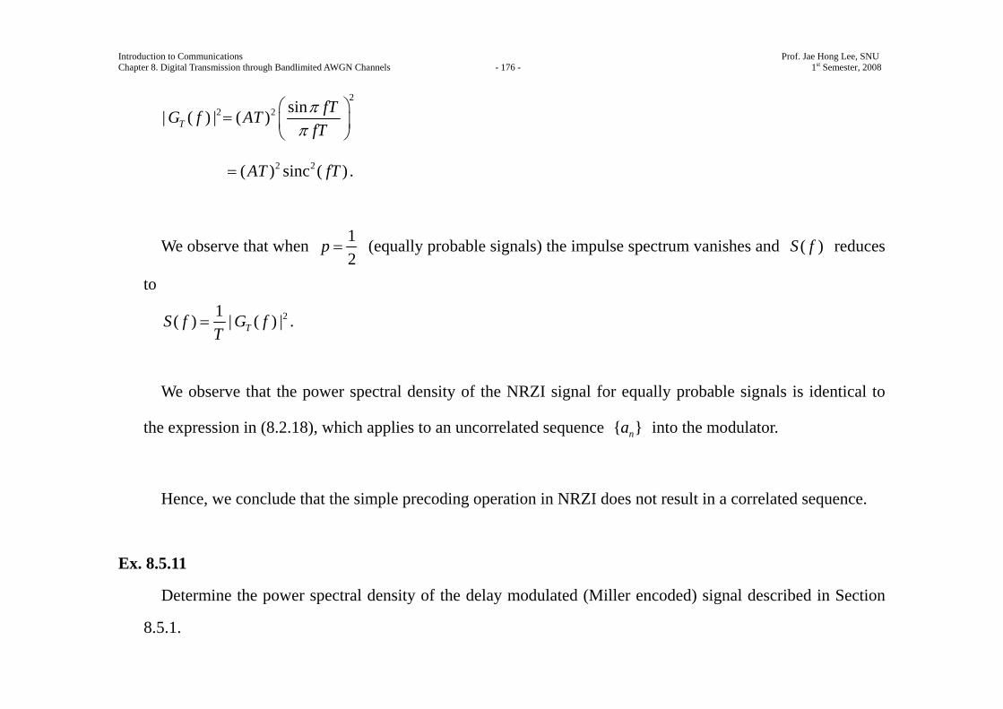
Introduction to Communications Prof. Jae Hong Lee, SNU Chapter 8. Digital Transmission through Bandlimited AWGN Channels - 176 - 1st Semester, 2008
22 2 sin| ( ) | ( )T
fTG f ATfTπ
π⎛ ⎞
= ⎜ ⎟⎝ ⎠
2 2( ) sinc ( )AT fT= .
We observe that when 12
p = (equally probable signals) the impulse spectrum vanishes and ( )S f reduces
to
21( ) | ( ) |TS f G fT
= .
We observe that the power spectral density of the NRZI signal for equally probable signals is identical to
the expression in (8.2.18), which applies to an uncorrelated sequence { }na into the modulator.
Hence, we conclude that the simple precoding operation in NRZI does not result in a correlated sequence.
Ex. 8.5.11
Determine the power spectral density of the delay modulated (Miller encoded) signal described in Section
8.5.1.
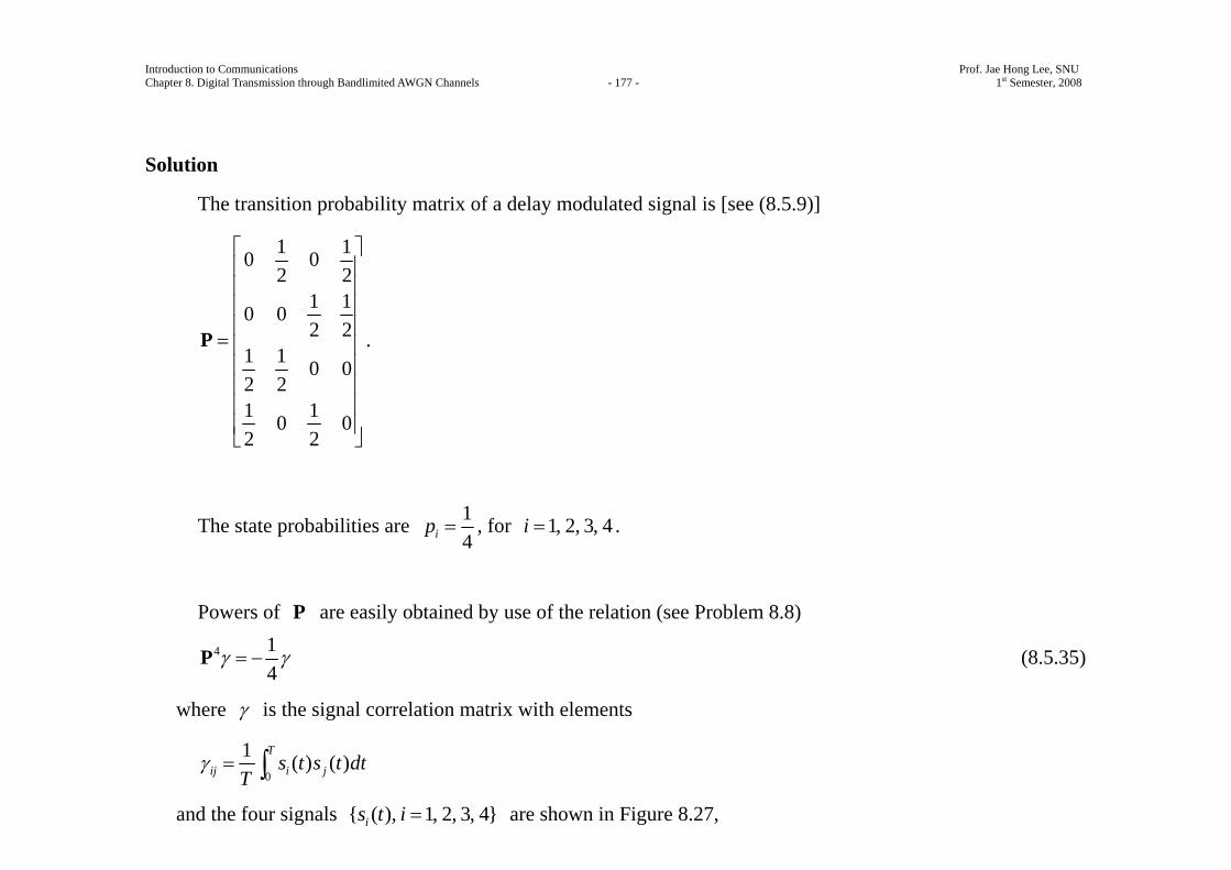
Introduction to Communications Prof. Jae Hong Lee, SNU Chapter 8. Digital Transmission through Bandlimited AWGN Channels - 177 - 1st Semester, 2008
Solution
The transition probability matrix of a delay modulated signal is [see (8.5.9)]
1 10 02 2
1 10 02 2
1 1 0 02 21 10 02 2
⎡ ⎤⎢ ⎥⎢ ⎥⎢ ⎥⎢ ⎥
= ⎢ ⎥⎢ ⎥⎢ ⎥⎢ ⎥⎢ ⎥⎣ ⎦
P .
The state probabilities are 14ip = , for 1, 2, 3, 4i = .
Powers of P are easily obtained by use of the relation (see Problem 8.8)
4 14
γ γ= −P (8.5.35)
where γ is the signal correlation matrix with elements
0
1 ( ) ( )T
ij i js t s t dtT
γ = ∫
and the four signals { ( ), 1, 2, 3, 4}is t i = are shown in Figure 8.27,
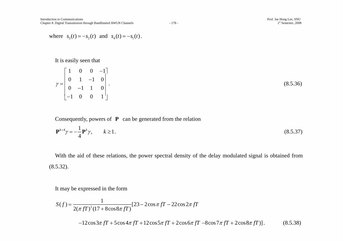
Introduction to Communications Prof. Jae Hong Lee, SNU Chapter 8. Digital Transmission through Bandlimited AWGN Channels - 178 - 1st Semester, 2008
where 3 2( ) ( )s t s t= − and 4 1( ) ( )s t s t= − .
It is easily seen that
1 0 0 10 1 1 00 1 1 01 0 0 1
γ
−⎡ ⎤⎢ ⎥−⎢ ⎥=⎢ ⎥−⎢ ⎥−⎣ ⎦
. (8.5.36)
Consequently, powers of P can be generated from the relation
4 1 , 14
k k kγ γ+ = − ≥P P . (8.5.37)
With the aid of these relations, the power spectral density of the delay modulated signal is obtained from
(8.5.32).
It may be expressed in the form
2
1( ) [23 2cos 22cos22( ) (17 8cos8 )
S f fT fTfT fT
π ππ π
= − −+
12cos3 5cos4 12cos5 2cos6fT fT fT fTπ π π π− + + + 8cos7 2cos8 )]fT fTπ π− + . (8.5.38)

Introduction to Communications Prof. Jae Hong Lee, SNU Chapter 8. Digital Transmission through Bandlimited AWGN Channels - 179 - 1st Semester, 2008
The power-spectral densities of the NRZI and the delay modulated signal are shown in Figure 8.32.
Figure 8.32 Power-spectral density (one-sided) of Miller code (delay modulation), and NRZ/NRZI baseband signals.
Introduction to Communications Prof. Jae Hong Lee, SNU Chapter 8. Digital Transmission through Bandlimited AWGN Channels - 180 - 1st Semester, 2008
We observe that the NRZI signal has a lowpass power spectral density with a peak of 0f = .
On the other hand, the delay modulated signal has very little power in the vicinity of 0f = .
It also has a relatively narrow power-spectral density.
These two characteristics make it particularly suitable for use in magnetic recording storage channels which
use flux-sensing heads for writing on and reading off a disk.
Also shown for comparison in Figure 8.32 is the power-spectral density of the modulated signal generated
by a ( , ) (2, 7)d κ = code followed by NRZI.
The (2, 7) runlength-limited code, previously given in Table 8.5, is also widely used in magnetic recording
channels.
When there is no memory in the modulation method, the signal waveform transmitted in each signaling
interval is independent of the waveforms transmitted in previous signaling intervals.
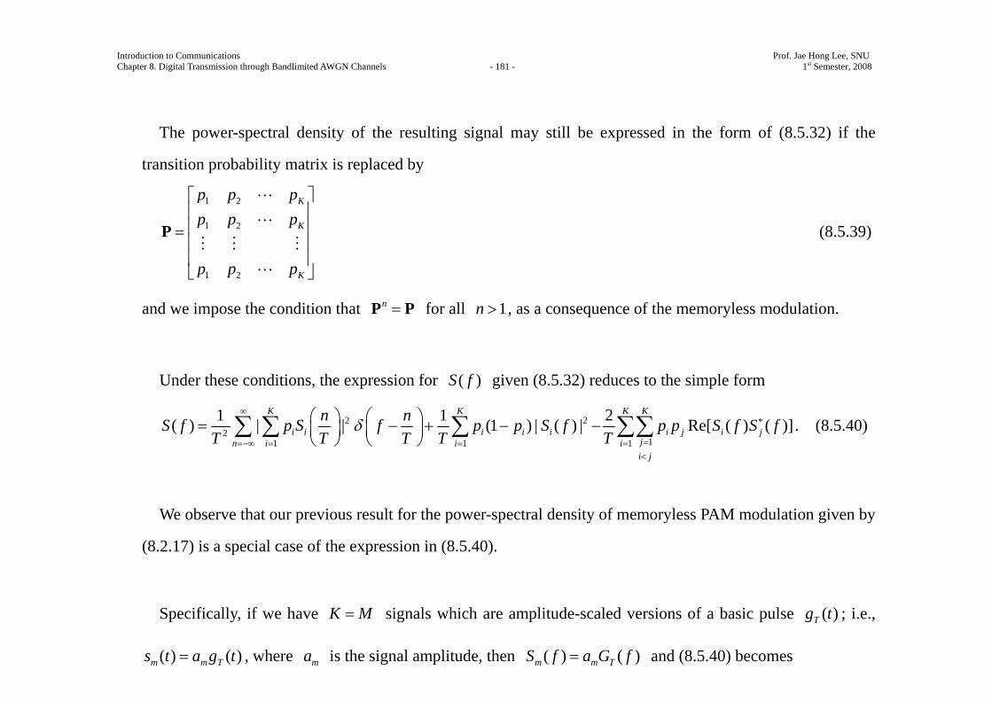
Introduction to Communications Prof. Jae Hong Lee, SNU Chapter 8. Digital Transmission through Bandlimited AWGN Channels - 181 - 1st Semester, 2008
The power-spectral density of the resulting signal may still be expressed in the form of (8.5.32) if the
transition probability matrix is replaced by
1 2
1 2
1 2
K
K
K
p p pp p p
p p p
⎡ ⎤⎢ ⎥⎢ ⎥=⎢ ⎥⎢ ⎥⎣ ⎦
P (8.5.39)
and we impose the condition that n =P P for all 1n > , as a consequence of the memoryless modulation.
Under these conditions, the expression for ( )S f given (8.5.32) reduces to the simple form
2 22
1 1
1 1( ) | | (1 ) | ( ) |K K
i i i i in i i
n nS f p S f p p S fT T T T
δ∞
=−∞ = =
⎛ ⎞ ⎛ ⎞= − + −⎜ ⎟ ⎜ ⎟⎝ ⎠ ⎝ ⎠
∑ ∑ ∑11
2 Re[ ( ) ( )]K K
i j i jjii j
p p S f S fT
∗
==<
− ∑∑ . (8.5.40)
We observe that our previous result for the power-spectral density of memoryless PAM modulation given by
(8.2.17) is a special case of the expression in (8.5.40).
Specifically, if we have K M= signals which are amplitude-scaled versions of a basic pulse ( )Tg t ; i.e.,
( ) ( )m m Ts t a g t= , where ma is the signal amplitude, then ( ) ( )m m TS f a G f= and (8.5.40) becomes
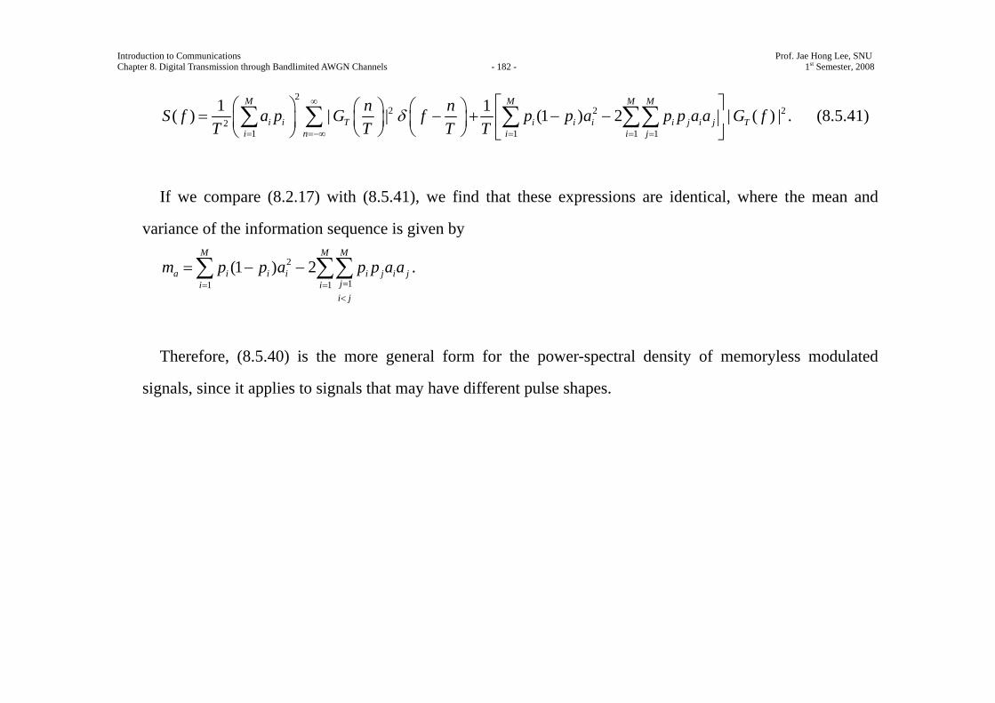
Introduction to Communications Prof. Jae Hong Lee, SNU Chapter 8. Digital Transmission through Bandlimited AWGN Channels - 182 - 1st Semester, 2008
22
21
1( ) | |M
i i Ti n
n nS f a p G fT T T
δ∞
= =−∞
⎛ ⎞ ⎛ ⎞ ⎛ ⎞= −⎜ ⎟ ⎜ ⎟⎜ ⎟ ⎝ ⎠ ⎝ ⎠⎝ ⎠∑ ∑ 2 2
1 1 1
1 (1 ) 2 | ( ) |M M M
i i i i j i j Ti i j
p p a p p a a G fT = = =
⎡ ⎤+ − −⎢ ⎥
⎣ ⎦∑ ∑∑ . (8.5.41)
If we compare (8.2.17) with (8.5.41), we find that these expressions are identical, where the mean and
variance of the information sequence is given by
2
11 1
(1 ) 2M M M
a i i i i j i jji ii j
m p p a p p a a== =<
= − −∑ ∑∑ .
Therefore, (8.5.40) is the more general form for the power-spectral density of memoryless modulated
signals, since it applies to signals that may have different pulse shapes.
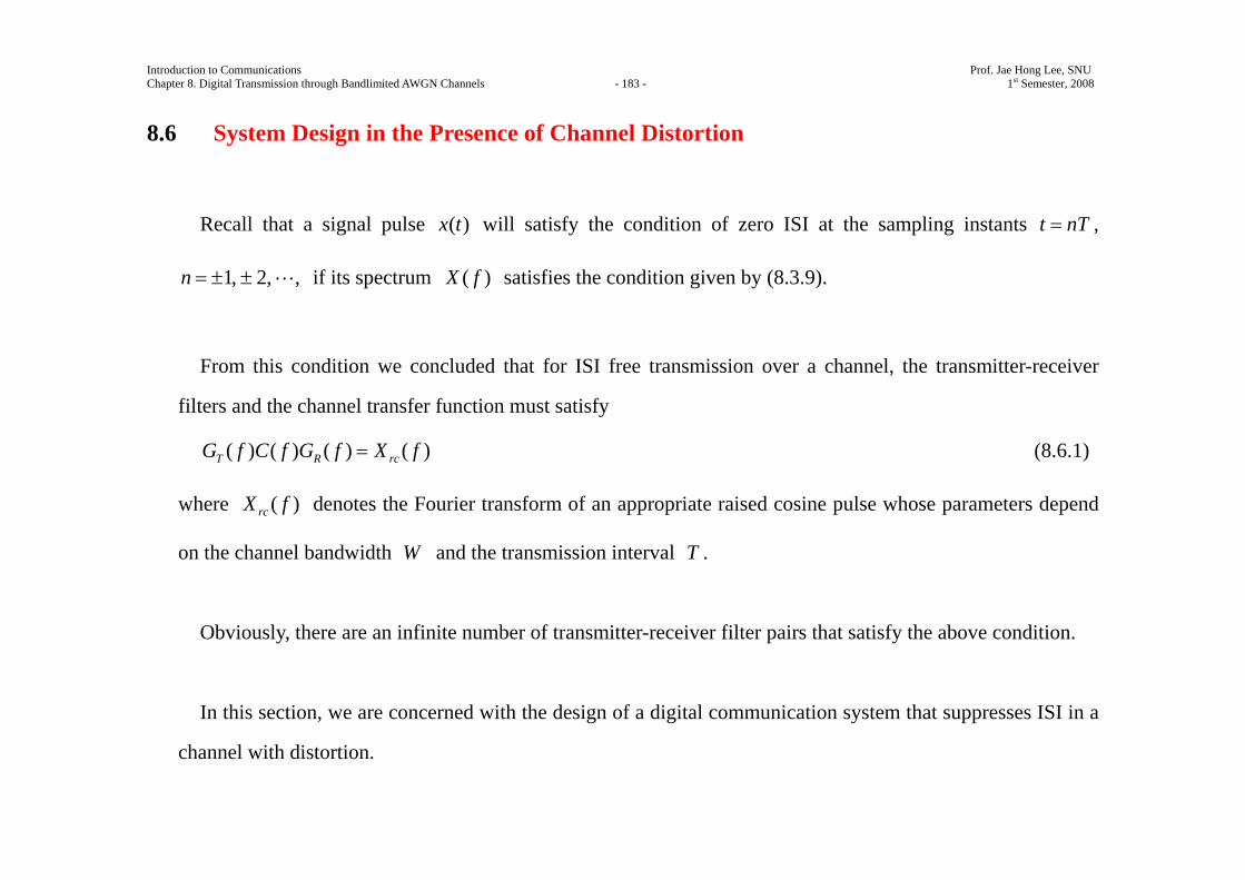
Introduction to Communications Prof. Jae Hong Lee, SNU Chapter 8. Digital Transmission through Bandlimited AWGN Channels - 183 - 1st Semester, 2008
8.6 System Design in the Presence of Channel Distortion
Recall that a signal pulse ( )x t will satisfy the condition of zero ISI at the sampling instants t nT= ,
1, 2, ,n = ± ± if its spectrum ( )X f satisfies the condition given by (8.3.9).
From this condition we concluded that for ISI free transmission over a channel, the transmitter-receiver
filters and the channel transfer function must satisfy
( ) ( ) ( ) ( )T R rcG f C f G f X f= (8.6.1)
where ( )rcX f denotes the Fourier transform of an appropriate raised cosine pulse whose parameters depend
on the channel bandwidth W and the transmission interval T .
Obviously, there are an infinite number of transmitter-receiver filter pairs that satisfy the above condition.
In this section, we are concerned with the design of a digital communication system that suppresses ISI in a
channel with distortion.
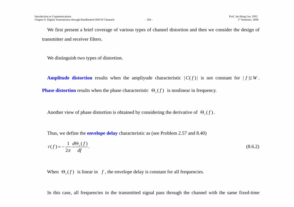
Introduction to Communications Prof. Jae Hong Lee, SNU Chapter 8. Digital Transmission through Bandlimited AWGN Channels - 184 - 1st Semester, 2008
We first present a brief coverage of various types of channel distortion and then we consider the design of
transmitter and receiver filters.
We distinguish two types of distortion.
Amplitude distortion results when the ampliyude characteristic | ( ) |C f is not constant for | |f W≤ .
Phase distortion results when the phase characteristic ( )c fΘ is nonlinear in frequency.
Another view of phase distortion is obtained by considering the derivative of ( )c fΘ .
Thus, we define the envelope delay characteristic as (see Problem 2.57 and 8.40)
1 ( )( )2
cd ffdf
τπ
Θ= − . (8.6.2)
When ( )c fΘ is linear in f , the envelope delay is constant for all frequencies.
In this case, all frequencies in the transmitted signal pass through the channel with the same fixed-time
Introduction to Communications Prof. Jae Hong Lee, SNU Chapter 8. Digital Transmission through Bandlimited AWGN Channels - 185 - 1st Semester, 2008
delay.
In such a case, there is no phase distortion.
However, when ( )c fΘ is nonlinear, the envelope delay ( )fτ varies with frequency and the various
frequency components in the input signal undergo different delays in passing through the channel.
In such a case we say that the transmitted signal has suffered from delay distortion.
Both amplitude and delay distortion cause intersymbol interference in the received signal.
For example, let us assume that we have designed a pulse with a raised cosine spectrum that has zero ISI at
the sampling instants.
An example of such a pulse is shown in Figure 8.33(a).
When the pulse is passed through a channel filter with constant amplitude | ( ) | 1C f = for | |f W< and a
Introduction to Communications Prof. Jae Hong Lee, SNU Chapter 8. Digital Transmission through Bandlimited AWGN Channels - 186 - 1st Semester, 2008
quadratic phase characteristic (linear envelope delay), the received pulse at the output of the channel is shown
in Figure 8.33(b).
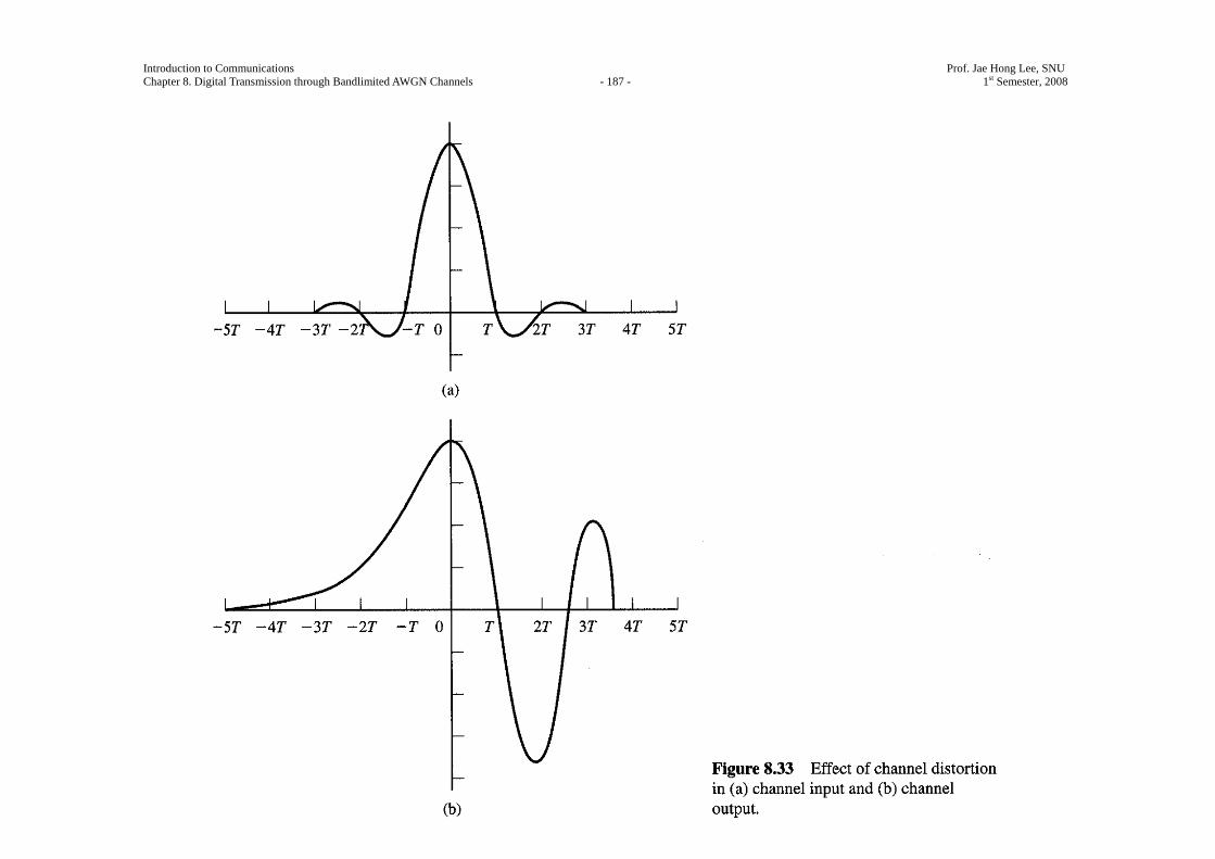
Introduction to Communications Prof. Jae Hong Lee, SNU Chapter 8. Digital Transmission through Bandlimited AWGN Channels - 187 - 1st Semester, 2008
Introduction to Communications Prof. Jae Hong Lee, SNU Chapter 8. Digital Transmission through Bandlimited AWGN Channels - 188 - 1st Semester, 2008
Note that the periodic zero crossing have been shifted by the delay distortion, so that the resulting pulse
suffers from ISI.
Consequently, a sequence of successive pulse would be smeared into one another and the peaks of the
pulses would no longer be distinguishable due to the ISI.
Next, we consider two problems.
First, we consider the design of transmitting and receiving filters in the presence of channel distortion when
the channel characteristics are known.
Second, we consider the design of special filters, called channel equalizers, that automatically and
adaptively correct for the channel distortion when the channel characteristics; i.e., | ( ) |C f and ( )c f∠Θ , are
known.
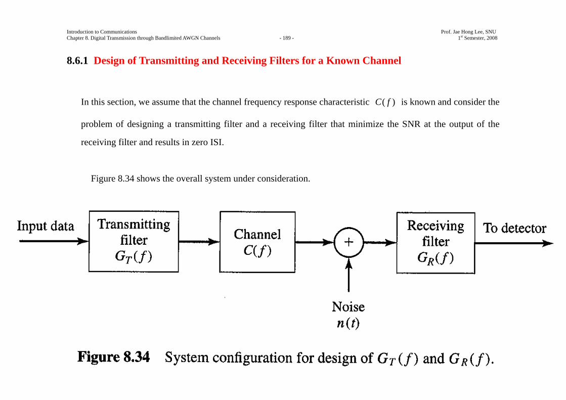
Introduction to Communications Prof. Jae Hong Lee, SNU Chapter 8. Digital Transmission through Bandlimited AWGN Channels - 189 - 1st Semester, 2008
8.6.1 Design of Transmitting and Receiving Filters for a Known Channel
In this section, we assume that the channel frequency response characteristic ( )C f is known and consider the
problem of designing a transmitting filter and a receiving filter that minimize the SNR at the output of the
receiving filter and results in zero ISI.
Figure 8.34 shows the overall system under consideration.
Introduction to Communications Prof. Jae Hong Lee, SNU Chapter 8. Digital Transmission through Bandlimited AWGN Channels - 190 - 1st Semester, 2008
For the signal component, we must satisfy the condition
0( ) ( ) ( ) ( ) j ftT R rcG f C f G f X f e π−= , | |f W≤ , (8.6.3)
where ( )rcX f is the desired raised cosine spectrum that yields zsro ISI at the sampling instants, and
0t is a time delay which is necessary to ensure the physical realizability og the transmitter and receiver filters.
The noise at the output of the receiving filter may be expressed as
( ) ( ) ( )Rv t n t g dτ τ τ∞
−∞= −∫ (8.6.4)
where ( )n t is the input to the filter.
The noise ( )n t is assumed to be zero-mean Gaussian.
Hence, ( )v t is zero-mean Gaussian, with a power-spectral density
2( ) ( ) | ( ) |v n RS f S f G f= (8.6.5)
where ( )nS f is the spectral density of the noise process ( )n t .
Introduction to Communications Prof. Jae Hong Lee, SNU Chapter 8. Digital Transmission through Bandlimited AWGN Channels - 191 - 1st Semester, 2008
For simplicity, we consider binary PAM transmission.
Then, the sampled output of the matched filter is
0m m my x a v= +
m ma v= + (8.6.6)
where 0x is normalized to unity,
ma d= ± , and
mv represents the noise term which is zero-mean Gaussian with variance
2 2( ) | ( ) |v n RS f G F dfσ∞
−∞= ∫ . (8.6.7)
Consequently, the probability of error is given by 2
22
12
v
y
dP e dyσπ∞ −
= ∫
2
2v
dQσ
⎛ ⎞= ⎜ ⎟⎜ ⎟
⎝ ⎠. (8.6.8)
Introduction to Communications Prof. Jae Hong Lee, SNU Chapter 8. Digital Transmission through Bandlimited AWGN Channels - 192 - 1st Semester, 2008
Now, suppose that we select the filter at the transmitter to have the frequency response
02( )( )
( )j ftrc
T
X fG f e
C fπ−= (8.6.9)
where 0t is a suitable delay to ensure causality.
Then, the cascade of the transmit filter and the channel results in the frequency response
02( ) ( ) ( ) j ftT rcG f C f X f e π−= . (8.6.10)
In the presence of additive white Gaussian noise, the filter at the receiver is designed to be matched to the
received signal pulse.
Hence, its frequency response
2( ) ( ) rj ftR rcG f X f e π−= (8.6.11)
where rt is an appropriate delay.
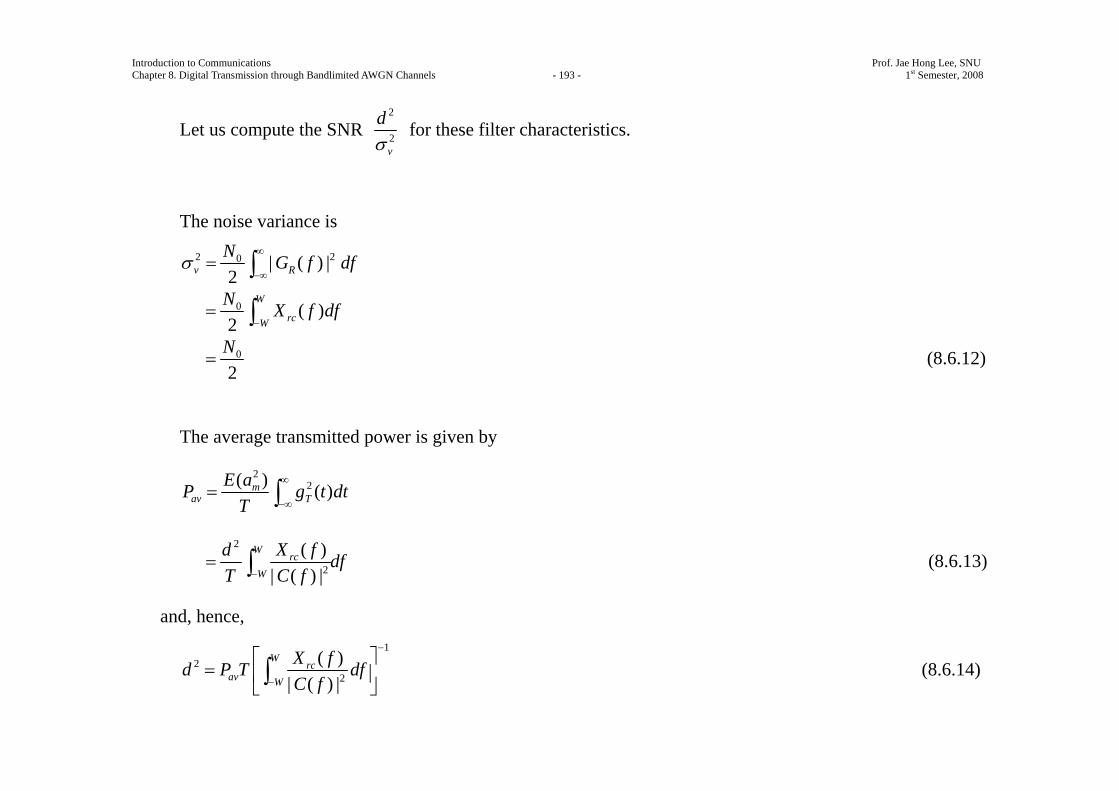
Introduction to Communications Prof. Jae Hong Lee, SNU Chapter 8. Digital Transmission through Bandlimited AWGN Channels - 193 - 1st Semester, 2008
Let us compute the SNR 2
2v
dσ
for these filter characteristics.
The noise variance is
2 20 | ( ) |2v RN G f dfσ
∞
−∞= ∫
0 ( )2
W
rcW
N X f df−
= ∫
0
2N
= (8.6.12)
The average transmitted power is given by
22( ) ( )m
av TE aP g t dt
T∞
−∞= ∫
2
2
( )| ( ) |
Wrc
W
d X f dfT C f−
= ∫ (8.6.13)
and, hence, 1
22
( )| ( ) |
Wrc
av W
X fd P T dfC f
−
−
⎡ ⎤= ⎢ ⎥
⎣ ⎦∫ (8.6.14)
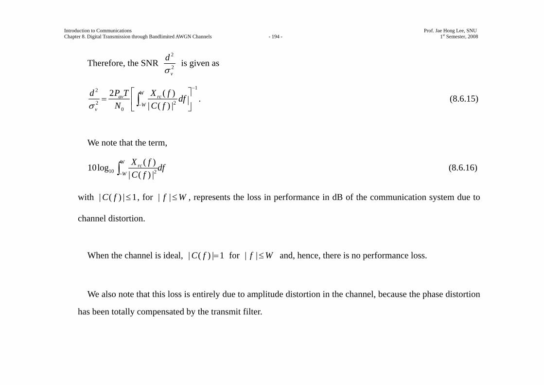
Introduction to Communications Prof. Jae Hong Lee, SNU Chapter 8. Digital Transmission through Bandlimited AWGN Channels - 194 - 1st Semester, 2008
Therefore, the SNR 2
2v
dσ
is given as
12
2 20
2 ( )| ( ) |
Wav rc
Wv
d P T X f dfN C fσ
−
−
⎡ ⎤= ⎢ ⎥
⎣ ⎦∫ . (8.6.15)
We note that the term,
10 2
( )10log| ( ) |
Wrc
W
X f dfC f−∫ (8.6.16)
with | ( ) | 1C f ≤ , for | |f W≤ , represents the loss in performance in dB of the communication system due to
channel distortion.
When the channel is ideal, | ( ) | 1C f = for | |f W≤ and, hence, there is no performance loss.
We also note that this loss is entirely due to amplitude distortion in the channel, because the phase distortion
has been totally compensated by the transmit filter.
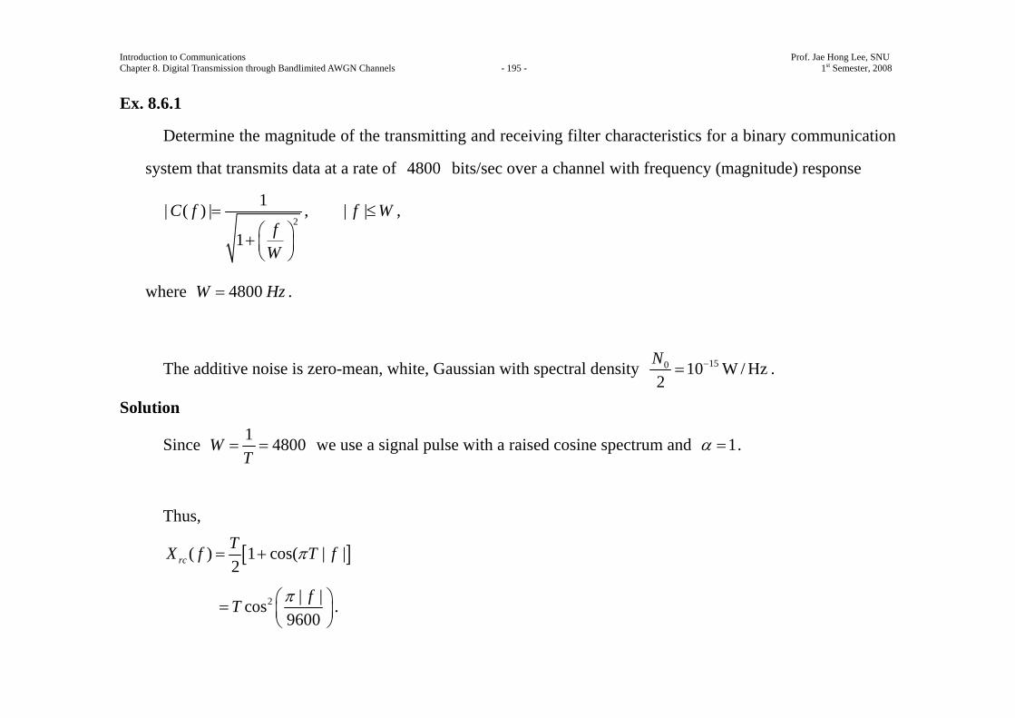
Introduction to Communications Prof. Jae Hong Lee, SNU Chapter 8. Digital Transmission through Bandlimited AWGN Channels - 195 - 1st Semester, 2008
Ex. 8.6.1
Determine the magnitude of the transmitting and receiving filter characteristics for a binary communication
system that transmits data at a rate of 4800 bits/sec over a channel with frequency (magnitude) response
2
1| ( ) |
1
C ff
W
=⎛ ⎞+ ⎜ ⎟⎝ ⎠
, | |f W≤ ,
where 4800W Hz= .
The additive noise is zero-mean, white, Gaussian with spectral density 150 10 W / Hz2N −= .
Solution
Since 1 4800WT
= = we use a signal pulse with a raised cosine spectrum and 1α = .
Thus,
[ ]( ) 1 cos( | |2rcTX f T fπ= +
2 | |cos9600
fT π⎛ ⎞= ⎜ ⎟⎝ ⎠
.
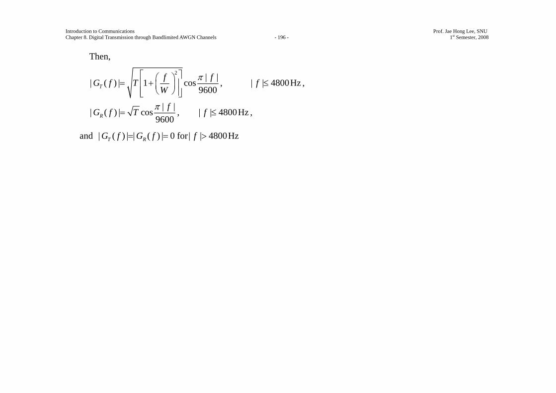
Introduction to Communications Prof. Jae Hong Lee, SNU Chapter 8. Digital Transmission through Bandlimited AWGN Channels - 196 - 1st Semester, 2008
Then, 2 | || ( ) | 1 cos
9600Tf fG f T
Wπ⎡ ⎤⎛ ⎞= +⎢ ⎥⎜ ⎟
⎝ ⎠⎢ ⎥⎣ ⎦, | | 4800Hzf ≤ ,
| || ( ) | cos9600R
fG f T π= , | | 4800Hzf ≤ ,
and | ( ) | | ( ) | 0 for| | 4800HzT RG f G f f= = >
Introduction to Communications Prof. Jae Hong Lee, SNU Chapter 8. Digital Transmission through Bandlimited AWGN Channels - 197 - 1st Semester, 2008
8.6.2 Channel Equalization
To design these transmitting and receiving filters for zero ISI at the sampling instants, the channel must be
precisely known and its characteristic should not change with time.
In practice we often encounter channels whose frequency response characteristics are either unknown or
change with time.
For example, in data transmission over the dial-up telephone network, the communication channel will be
different every time we dial a number, because the channel route will be different.
Once a connection is made, however, the channel will be time-invariant for a relatively long period of time.
This is an example of a channel whose characteristics are unknown a priori.
Examples of time-varying channels are radio channels, such as ionospheric propagation channels.
These channels are characterized by time-varying frequency response characteristics.
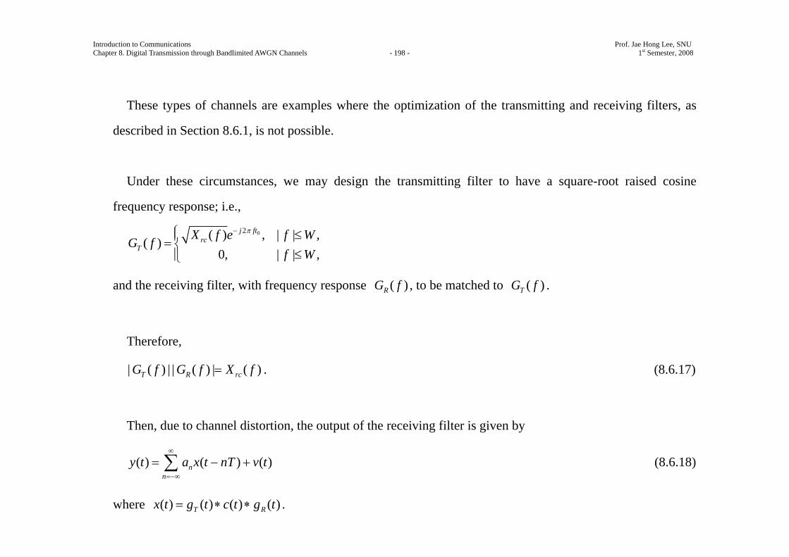
Introduction to Communications Prof. Jae Hong Lee, SNU Chapter 8. Digital Transmission through Bandlimited AWGN Channels - 198 - 1st Semester, 2008
These types of channels are examples where the optimization of the transmitting and receiving filters, as
described in Section 8.6.1, is not possible.
Under these circumstances, we may design the transmitting filter to have a square-root raised cosine
frequency response; i.e.,
02( ) , | | ,( )0, | | ,
j ftrc
TX f e f WG f
f W
π−⎧ ≤⎪= ⎨≤⎪⎩
and the receiving filter, with frequency response ( )RG f , to be matched to ( )TG f .
Therefore,
| ( ) | | ( ) | ( )T R rcG f G f X f= . (8.6.17)
Then, due to channel distortion, the output of the receiving filter is given by
( ) ( ) ( )nn
y t a x t nT v t∞
=−∞
= − +∑ (8.6.18)
where ( ) ( ) ( ) ( )T Rx t g t c t g t= ∗ ∗ .

Introduction to Communications Prof. Jae Hong Lee, SNU Chapter 8. Digital Transmission through Bandlimited AWGN Channels - 199 - 1st Semester, 2008
The filter output may be sampled periodically to produce the sequence
m n m n mn
y a x v∞
−=−∞
= +∑
0 m n m n mnn m
x a a x v+∞
−=−∞≠
= + +∑ (8.6.19)
where ( ), 0, 1, 2, .nx x nT n= = ± ±
The middle term on the right-hand side of (8.6.19) represents the ISI.
In any practical system, it is reasonable to assume that the ISI affects a finite number of symbols.
Hence, we may assume that 0nx = for 1n L< − and 2n L> ,
where 1L and 2L are finite, positive integers.
Consequently, the ISI observed at the output of the receiving filter may be viewed as being generated by
passing the data sequence { }ma through an FIR filter with coefficients 1 2{ , }nx L n L− ≤ ≤ ,
as shown in Figure 8.35 which is called the equivalent discrete-time channel filter.
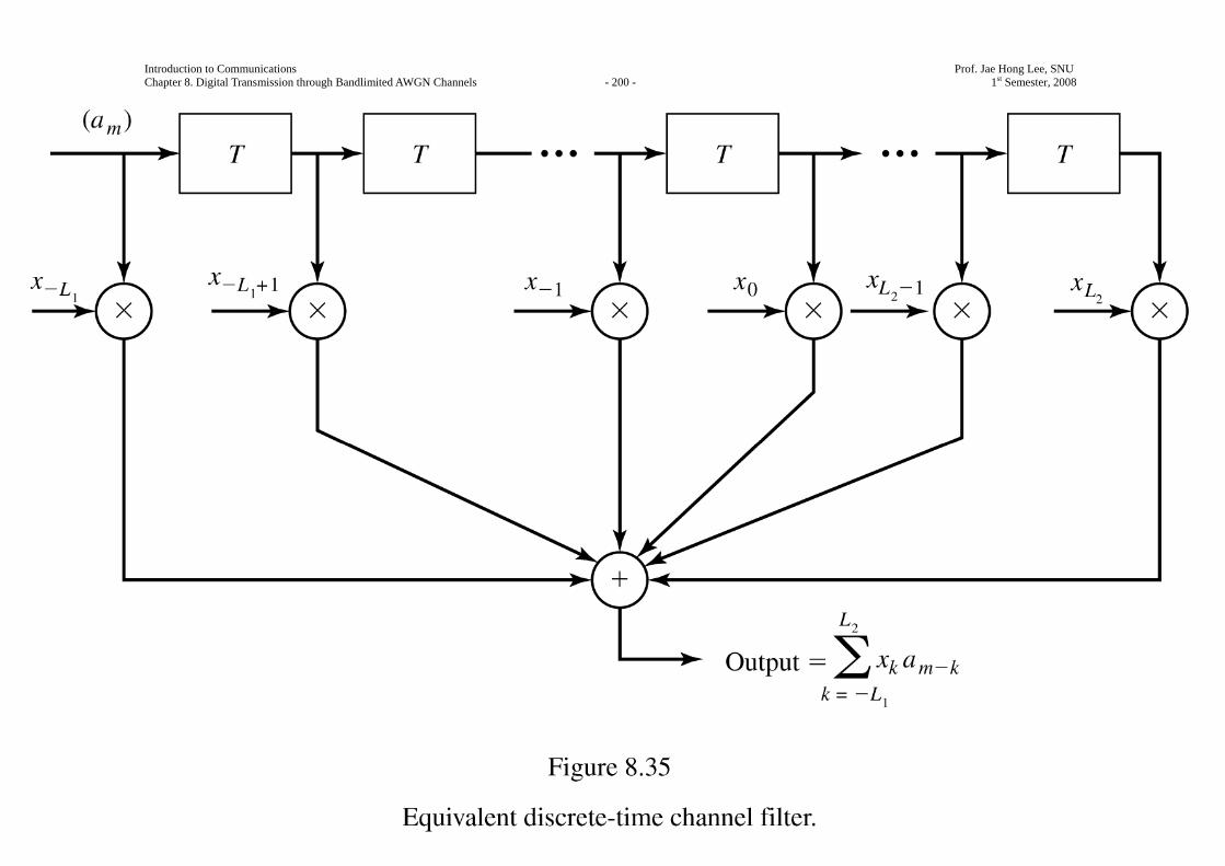
Introduction to Communications Prof. Jae Hong Lee, SNU Chapter 8. Digital Transmission through Bandlimited AWGN Channels - 200 - 1st Semester, 2008
Introduction to Communications Prof. Jae Hong Lee, SNU Chapter 8. Digital Transmission through Bandlimited AWGN Channels - 201 - 1st Semester, 2008
Since its input is the discrete information sequence (binary or M -art), the output of the discrete-time
channel filter may be characterized as the output of a finite-state machine corrupted by additive Gaussian noise.
Hence, the noise-free output of the filter is described by a trellis having LM states where 1 2L L L= + .
Maximum-Likelihood Sequence Detection
The optimum detector for the information sequence { }ma based oon the observation of the received
sequence { }my , given by (8.6.19), is a ML sequence detector.
The detector is akin to the ML sequence detector described in the context of detecting partial response
signals which have controlled ISI.
The Viterbi algorithm provides a method for searching through the trllis for the ML signal path.
To accomplish this search, the equivalent channel filter coefficients { }nx must be known or measured by
some method.

Introduction to Communications Prof. Jae Hong Lee, SNU Chapter 8. Digital Transmission through Bandlimited AWGN Channels - 202 - 1st Semester, 2008
At each stage of the trellis search, there are LM corresponding Euclidean distance path metrics.
Due to exponential increase in the computational complexity of the Viterbi algorithm with the span (length
L ) of the ISI, this type of detection is practical only when M and L are small.
For example in mobile cellular telephone systems which employ digital transmission of speech signals, M
is usually selected to be small; e.g., 2M = or 4, and 2 5L≤ ≤ .
In this case, the ML sequence detector may be implemented with reasonable complexity. However, when
M and L are large, the ML sequence detector becomes impractical.
In such a case other more practical but suboptimum methods are used to detect the information sequence
{ }ma in the presence of ISI.
Neverthless, the performance of the ML sequence detector for a channel with ISI serves as a benchmark
for comparing its performance with that of suboptimum methods.

Introduction to Communications Prof. Jae Hong Lee, SNU Chapter 8. Digital Transmission through Bandlimited AWGN Channels - 203 - 1st Semester, 2008
Two suboptimum methods are ddescribed below.
Linear Equalizers
To compensate for the channel distortion, we may employ a linear filter with adjustable parameters which is
called channel equalizers or, simply, equalizers.
The filter parameters are adjusted on the basis of measurements of the channel characteristics.
On channels whose frequency-response characteristics are unknown, but time-invariant, we may measure
the channel characteristics, adjust the parameters of the equalizer, and once adjusted, the parameters remain
fixed during the transmission of data.
Such equalizers are called preset equalizers.
On the other hand, adaptive equalizers update their parameters on a periodic basis during the transmission
of data.
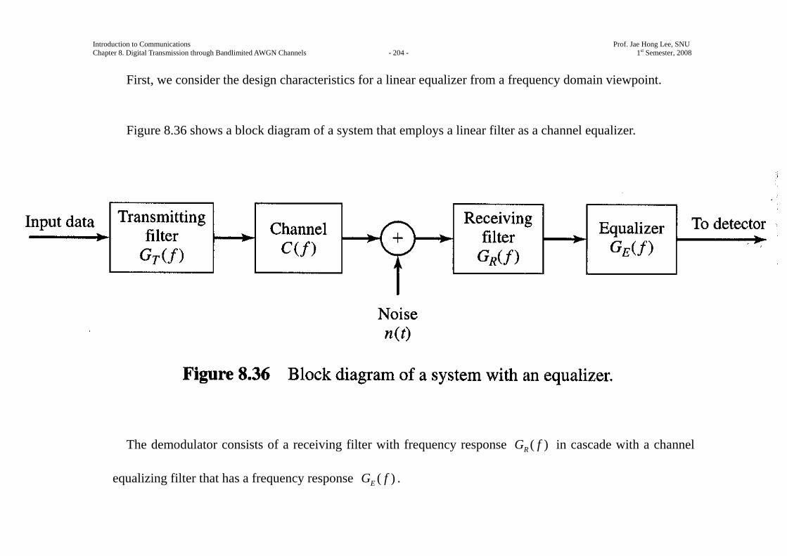
Introduction to Communications Prof. Jae Hong Lee, SNU Chapter 8. Digital Transmission through Bandlimited AWGN Channels - 204 - 1st Semester, 2008
First, we consider the design characteristics for a linear equalizer from a frequency domain viewpoint.
Figure 8.36 shows a block diagram of a system that employs a linear filter as a channel equalizer.
The demodulator consists of a receiving filter with frequency response ( )RG f in cascade with a channel
equalizing filter that has a frequency response ( )EG f .
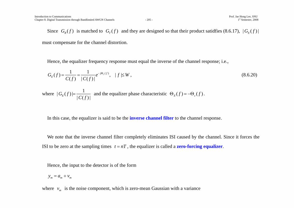
Introduction to Communications Prof. Jae Hong Lee, SNU Chapter 8. Digital Transmission through Bandlimited AWGN Channels - 205 - 1st Semester, 2008
Since ( )RG f is matched to ( )TG f and they are designed so that their product satidfies (8.6.17), | ( ) |EG f
must compensate for the channel distortion.
Hence, the equalizer frequency response must equal the inverse of the channel response; i.e.,
( )1 1( ) , | |( ) | ( ) |
cj fEG f e f W
C f C f− Θ= = ≤ , (8.6.20)
where 1| ( ) || ( ) |EG fC f
= and the equalizer phase characteristic ( ) ( )E cf fΘ = −Θ .
In this case, the equalizer is said to be the inverse channel filter to the channel response.
We note that the inverse channel filter completely eliminates ISI caused by the channel. Since it forces the
ISI to be zero at the sampling times t nT= , the equalizer is called a zero-forcing equalizer.
Hence, the input to the detector is of the form
m m my a v= +
where mv is the noise component, which is zero-mean Gaussian with a variance
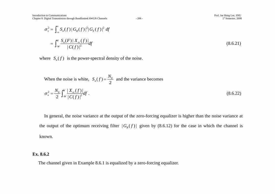
Introduction to Communications Prof. Jae Hong Lee, SNU Chapter 8. Digital Transmission through Bandlimited AWGN Channels - 206 - 1st Semester, 2008
2 2 2( ) | ( ) | | ( ) |v n R ES f G f G f dfσ∞
−∞= ∫
2
( ) | ( ) || ( ) |
Wn rc
W
S F X f dfC f−
= ∫ (8.6.21)
where ( )nS f is the power-spectral density of the noise.
When the noise is white, 0( )2nNS f = and the variance becomes
2 02
| ( ) |2 | ( ) |
Wrc
v W
N X f dfC f
σ−
= ∫ . (8.6.22)
In general, the noise variance at the output of the zero-forcing equalizer is higher than the noise variance at
the output of the optimum receiving filter | ( ) |RG f given by (8.6.12) for the case in which the channel is
known.
Ex. 8.6.2
The channel given in Example 8.6.1 is equalized by a zero-forcing equalizer.
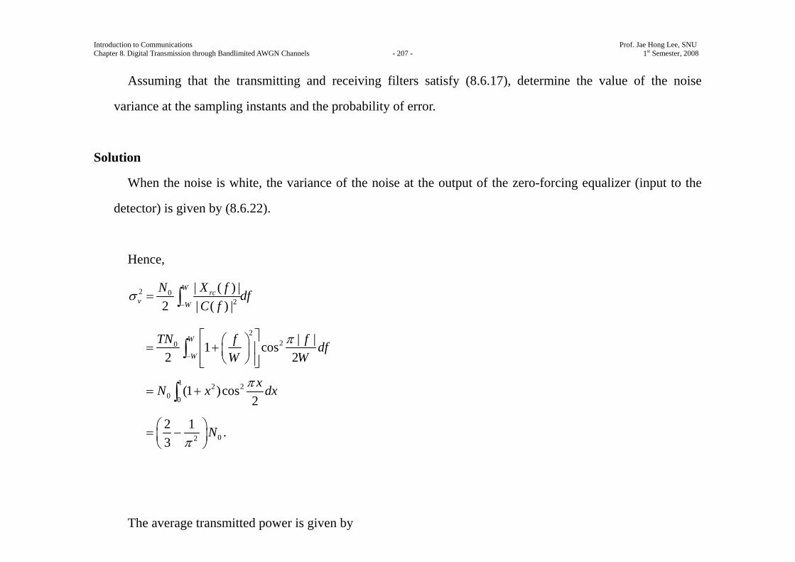
Introduction to Communications Prof. Jae Hong Lee, SNU Chapter 8. Digital Transmission through Bandlimited AWGN Channels - 207 - 1st Semester, 2008
Assuming that the transmitting and receiving filters satisfy (8.6.17), determine the value of the noise
variance at the sampling instants and the probability of error.
Solution
When the noise is white, the variance of the noise at the output of the zero-forcing equalizer (input to the
detector) is given by (8.6.22).
Hence,
2 02
| ( ) |2 | ( ) |
Wrc
v W
N X f dfC f
σ−
= ∫
220 | |1 cos
2 2W
W
TN f f dfW W
π−
⎡ ⎤⎛ ⎞= +⎢ ⎥⎜ ⎟⎝ ⎠⎢ ⎥⎣ ⎦
∫
1 2 20 0
(1 )cos2xN x dxπ
= +∫
02
2 13
Nπ
⎛ ⎞= −⎜ ⎟⎝ ⎠
.
The average transmitted power is given by
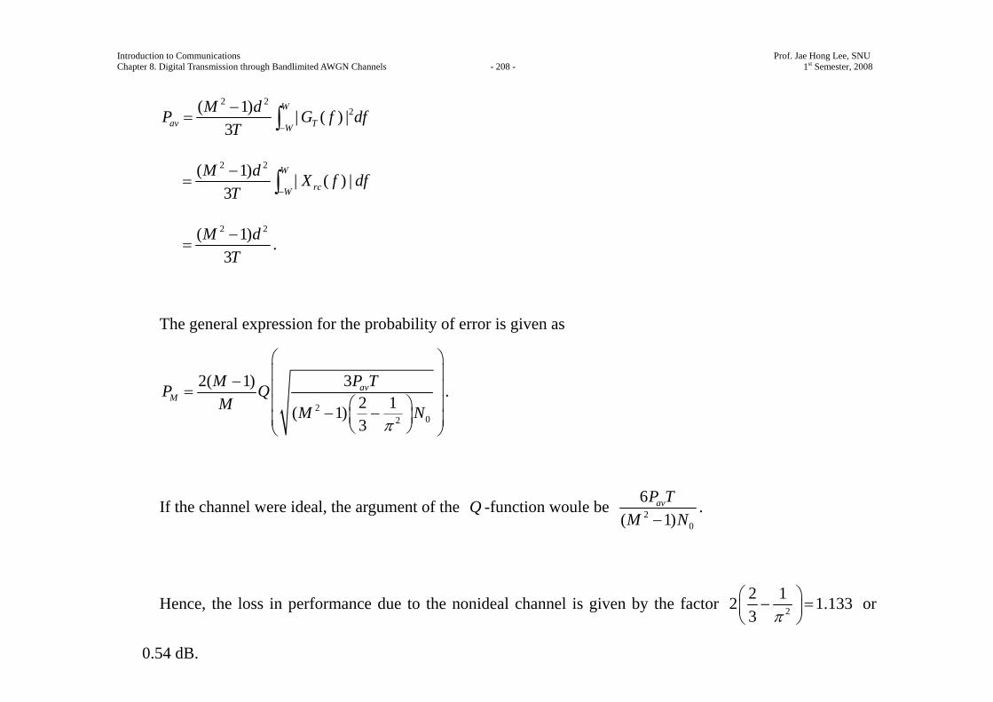
Introduction to Communications Prof. Jae Hong Lee, SNU Chapter 8. Digital Transmission through Bandlimited AWGN Channels - 208 - 1st Semester, 2008
2 22( 1) | ( ) |
3W
av TW
M dP G f dfT −
−= ∫
2 2( 1) | ( ) |3
W
rcW
M d X f dfT −
−= ∫
2 2( 1)3
M dT−
= .
The general expression for the probability of error is given as
202
2( 1) 32 1( 1)3
avM
M P TP QM M N
π
⎛ ⎞⎜ ⎟− ⎜ ⎟=
⎛ ⎞⎜ ⎟− −⎜ ⎟⎜ ⎟⎝ ⎠⎝ ⎠
.
If the channel were ideal, the argument of the Q -function woule be 20
6( 1)
avP TM N−
.
Hence, the loss in performance due to the nonideal channel is given by the factor 2
2 12 1.1333 π
⎛ ⎞− =⎜ ⎟⎝ ⎠
or
0.54 dB.
Introduction to Communications Prof. Jae Hong Lee, SNU Chapter 8. Digital Transmission through Bandlimited AWGN Channels - 209 - 1st Semester, 2008
Consider the design of a linear equalizer from a time-domain view-point.
We noted previously that in real channels, the ISI is limited to a finite number of samples, say L samples.
As a consequence, in practice the channel equliaer is approximated by a finite duration impulse response
(FIR) filter, or transversal filter, with adjustable tap coefficients { }nc , as shown in Figure 8.37.
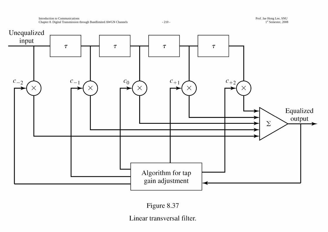
Introduction to Communications Prof. Jae Hong Lee, SNU Chapter 8. Digital Transmission through Bandlimited AWGN Channels - 210 - 1st Semester, 2008

Introduction to Communications Prof. Jae Hong Lee, SNU Chapter 8. Digital Transmission through Bandlimited AWGN Channels - 211 - 1st Semester, 2008
The time delay τ between asjacent taps may be selected as large as T , the symbol interval, in which case
the FIR equalizer is called a symbol-spaced equalizer.
In this case the input to the equalizer is the sampled sequence given by (8.6.19).
However, we note that when 1 2WT< , frequencies in the received signal above the folding frequency 1
T
are aliased into frequencies below 1T
.
In this case, the equalizer compensates for the aliased channel-distorted signal.
On the other hand, when the time delay τ between adjacent taps is selected such that 1 12WTτ
≥ ≥ , no
aliasing occurs and, hence, the inverse channel equalizer compensates for the true channel distortion.
Since Tτ < , the channel equalizer is said to have fractionally spaced taps and it is called a fractionally
spaced equalizer.
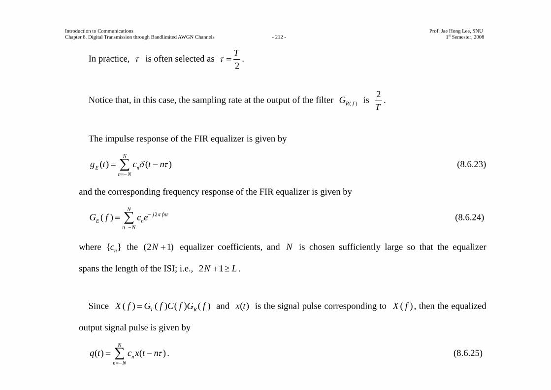
Introduction to Communications Prof. Jae Hong Lee, SNU Chapter 8. Digital Transmission through Bandlimited AWGN Channels - 212 - 1st Semester, 2008
In practice, τ is often selected as 2Tτ = .
Notice that, in this case, the sampling rate at the output of the filter ( )R fG is 2T
.
The impulse response of the FIR equalizer is given by
( ) ( )N
E nn N
g t c t nδ τ=−
= −∑ (8.6.23)
and the corresponding frequency response of the FIR equalizer is given by
2( )N
j fnE n
n N
G f c e π τ−
=−
= ∑ (8.6.24)
where { }nc the (2 1)N + equalizer coefficients, and N is chosen sufficiently large so that the equalizer
spans the length of the ISI; i.e., 2 1N L+ ≥ .
Since ( ) ( ) ( ) ( )T RX f G f C f G f= and ( )x t is the signal pulse corresponding to ( )X f , then the equalized
output signal pulse is given by
( ) ( )N
nn N
q t c x t nτ=−
= −∑ . (8.6.25)
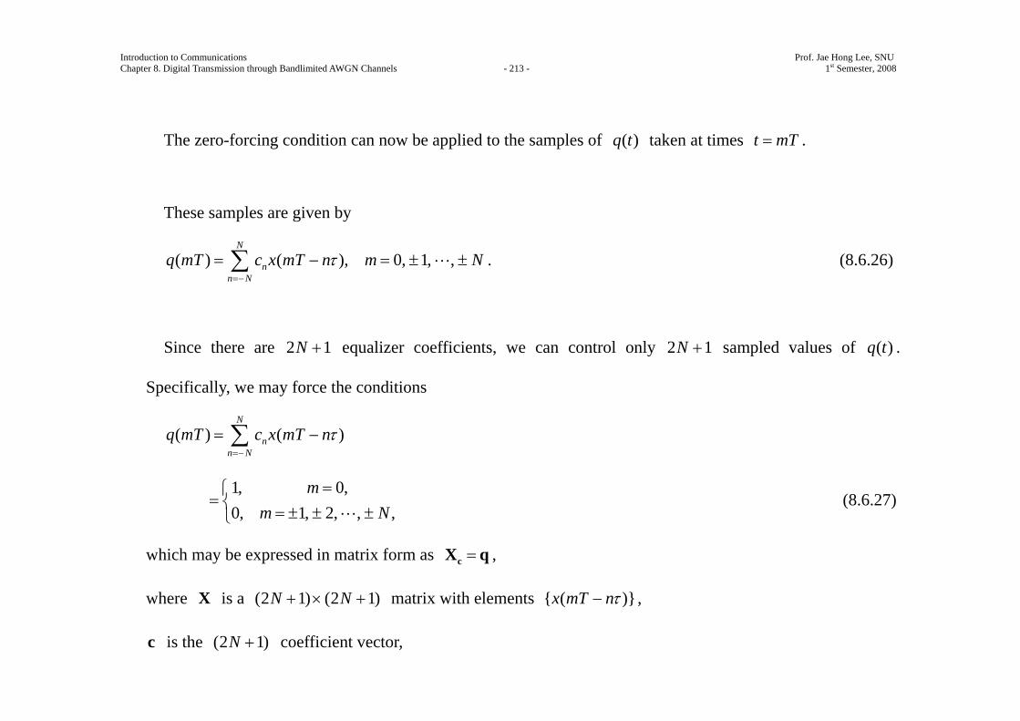
Introduction to Communications Prof. Jae Hong Lee, SNU Chapter 8. Digital Transmission through Bandlimited AWGN Channels - 213 - 1st Semester, 2008
The zero-forcing condition can now be applied to the samples of ( )q t taken at times t mT= .
These samples are given by
( ) ( ), 0, 1, ,N
nn N
q mT c x mT n m Nτ=−
= − = ± ±∑ . (8.6.26)
Since there are 2 1N + equalizer coefficients, we can control only 2 1N + sampled values of ( )q t .
Specifically, we may force the conditions
( ) ( )N
nn N
q mT c x mT nτ=−
= −∑
1, 0,0, 1, 2, , ,
mm N
=⎧= ⎨ = ± ± ±⎩
(8.6.27)
which may be expressed in matrix form as =cX q ,
where X is a (2 1) (2 1)N N+ × + matrix with elements { ( )}x mT nτ− ,
c is the (2 1)N + coefficient vector,
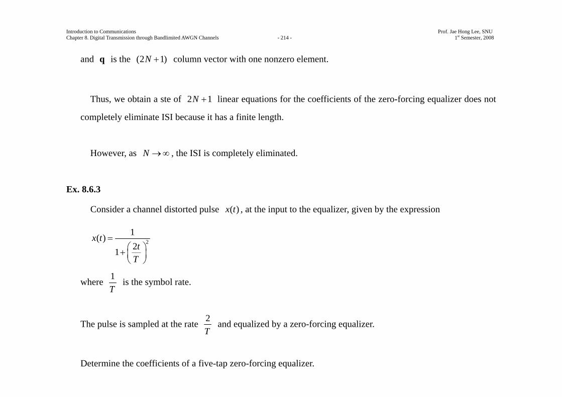
Introduction to Communications Prof. Jae Hong Lee, SNU Chapter 8. Digital Transmission through Bandlimited AWGN Channels - 214 - 1st Semester, 2008
and q is the (2 1)N + column vector with one nonzero element.
Thus, we obtain a ste of 2 1N + linear equations for the coefficients of the zero-forcing equalizer does not
completely eliminate ISI because it has a finite length.
However, as N →∞ , the ISI is completely eliminated.
Ex. 8.6.3
Consider a channel distorted pulse ( )x t , at the input to the equalizer, given by the expression
21( )21
x tt
T
=⎛ ⎞+ ⎜ ⎟⎝ ⎠
where 1T
is the symbol rate.
The pulse is sampled at the rate 2T
and equalized by a zero-forcing equalizer.
Determine the coefficients of a five-tap zero-forcing equalizer.
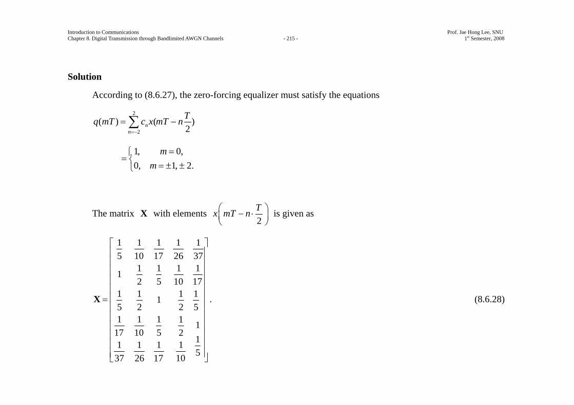
Introduction to Communications Prof. Jae Hong Lee, SNU Chapter 8. Digital Transmission through Bandlimited AWGN Channels - 215 - 1st Semester, 2008
Solution
According to (8.6.27), the zero-forcing equalizer must satisfy the equations
2
2
( ) ( )2n
n
Tq mT c x mT n=−
= −∑
1, 0,0, 1, 2.
mm
=⎧= ⎨ = ± ±⎩
The matrix X with elements 2Tx mT n⎛ ⎞− ⋅⎜ ⎟
⎝ ⎠ is given as
1 1 1 1 15 10 17 26 37
1 1 1 112 5 10 17
1 1 1 115 2 2 51 1 1 1 1
17 10 5 2111 1 151037 26 17
⎡ ⎤⎢ ⎥⎢ ⎥⎢ ⎥⎢ ⎥⎢ ⎥⎢ ⎥=⎢ ⎥⎢ ⎥⎢ ⎥⎢ ⎥⎢ ⎥⎢ ⎥⎣ ⎦
X . (8.6.28)
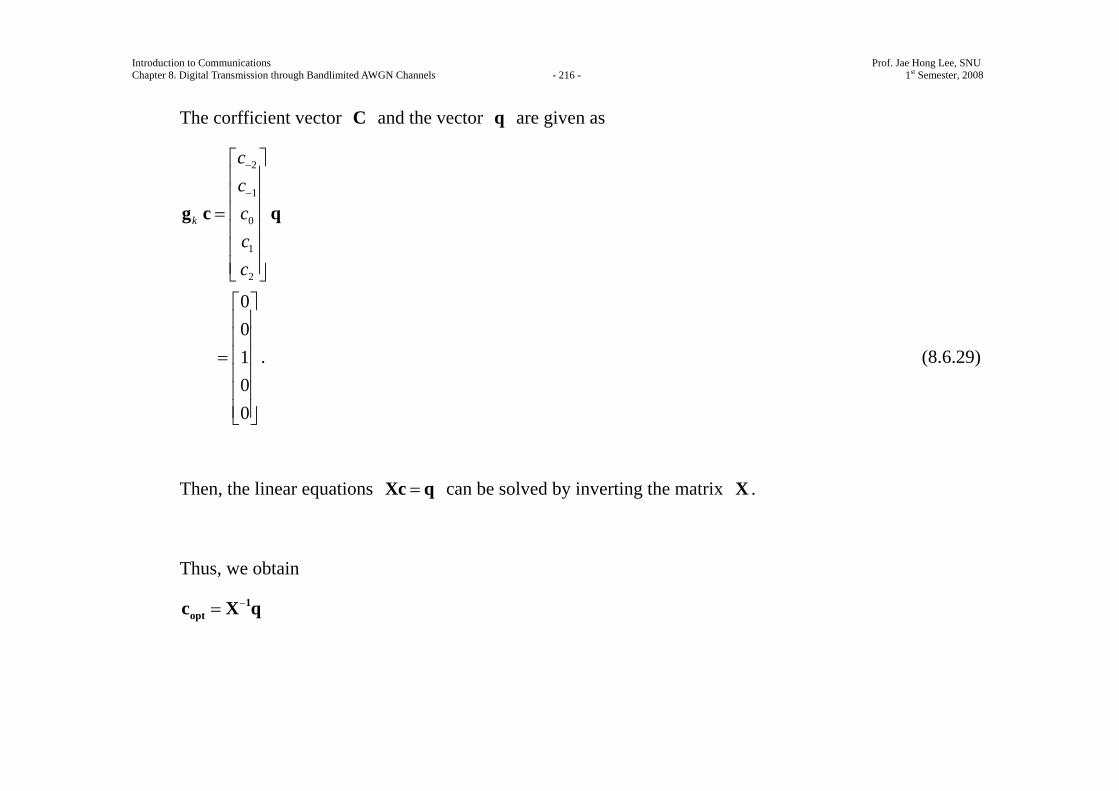
Introduction to Communications Prof. Jae Hong Lee, SNU Chapter 8. Digital Transmission through Bandlimited AWGN Channels - 216 - 1st Semester, 2008
The corfficient vector C and the vector q are given as
kg
2
1
0
1
2
ccccc
−
−
⎡ ⎤⎢ ⎥⎢ ⎥⎢ ⎥=⎢ ⎥⎢ ⎥⎢ ⎥⎣ ⎦
c q
00100
⎡ ⎤⎢ ⎥⎢ ⎥⎢ ⎥=⎢ ⎥⎢ ⎥⎢ ⎥⎣ ⎦
. (8.6.29)
Then, the linear equations =Xc q can be solved by inverting the matrix X .
Thus, we obtain
−= 1optc X q
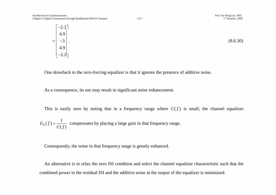
Introduction to Communications Prof. Jae Hong Lee, SNU Chapter 8. Digital Transmission through Bandlimited AWGN Channels - 217 - 1st Semester, 2008
2.24.9
34.92.2
−⎡ ⎤⎢ ⎥⎢ ⎥⎢ ⎥= −⎢ ⎥⎢ ⎥⎢ ⎥−⎣ ⎦
. (8.6.30)
One drawback to the zero-forcing equalizer is that it ignores the presence of additive noise.
As a consequence, its use may result in significant noise enhancement.
This is easily seen by noting that in a frequency range where ( )C f is small, the channel equalizer
1( )( )EG f
C f= compensates by placing a large gain in that frequency range.
Consequently, the noise in that frequency tange is greatly enhanced.
An alternative is to relax the zero ISI condition and select the channel equalizer characteristic such that the
combined power in the residual ISI and the additive noise at the output of the equalizer is minimized.

Introduction to Communications Prof. Jae Hong Lee, SNU Chapter 8. Digital Transmission through Bandlimited AWGN Channels - 218 - 1st Semester, 2008
A channel equalizer that is optimized based on the minimum mean-square-error (MMSE) criterion
accomplishes the desired goal.
To elaborate, let us consider the noise-corrupted output of the FIR equalizer which is given by
( ) ( )N
nn N
z t c y t nτ=−
= −∑ (8.6.31)
where ( )y t is the input to the equalizer, given by (8.6.18).
The output is sampled at times t mT= .
Thus, we obtain
( ) ( )N
nn N
z mT c y mT nτ=−
= −∑ . (8.6.32)
The desired response sample at the output of the equalizer at t mT= is the transmitted symbol ma is
given by
2MSE [ ( ) ]mE z mT a= −
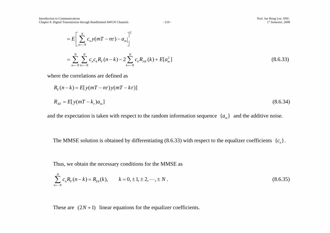
Introduction to Communications Prof. Jae Hong Lee, SNU Chapter 8. Digital Transmission through Bandlimited AWGN Channels - 219 - 1st Semester, 2008
2
( )N
n mn N
E c y mT n aτ=−
⎡ ⎤= − −⎢ ⎥⎣ ⎦
∑
2( ) 2 ( ) [ ]N N N
n k Y k AY mn N k N k N
c c R n k c R k E a=− =− =−
= − − +∑ ∑ ∑ (8.6.33)
where the correlations are defined as
( ) [ ( ) ( )]YR n k E y mT n y mT kτ τ− = − −
[ ( ) ]AY mR E y mT k aτ= − (8.6.34)
and the expectation is taken with respect to the random information sequence { }ma and the additive noise.
The MMSE solution is obtained by differentiating (8.6.33) with respect to the equalizer coefficients { }nc .
Thus, we obtain the necessary conditions for the MMSE as
( ) ( ), 0, 1, 2, ,N
n Y YAn N
c R n k R k k N=−
− = = ± ± ±∑ . (8.6.35)
These are (2 1)N + linear equations for the equalizer coefficients.
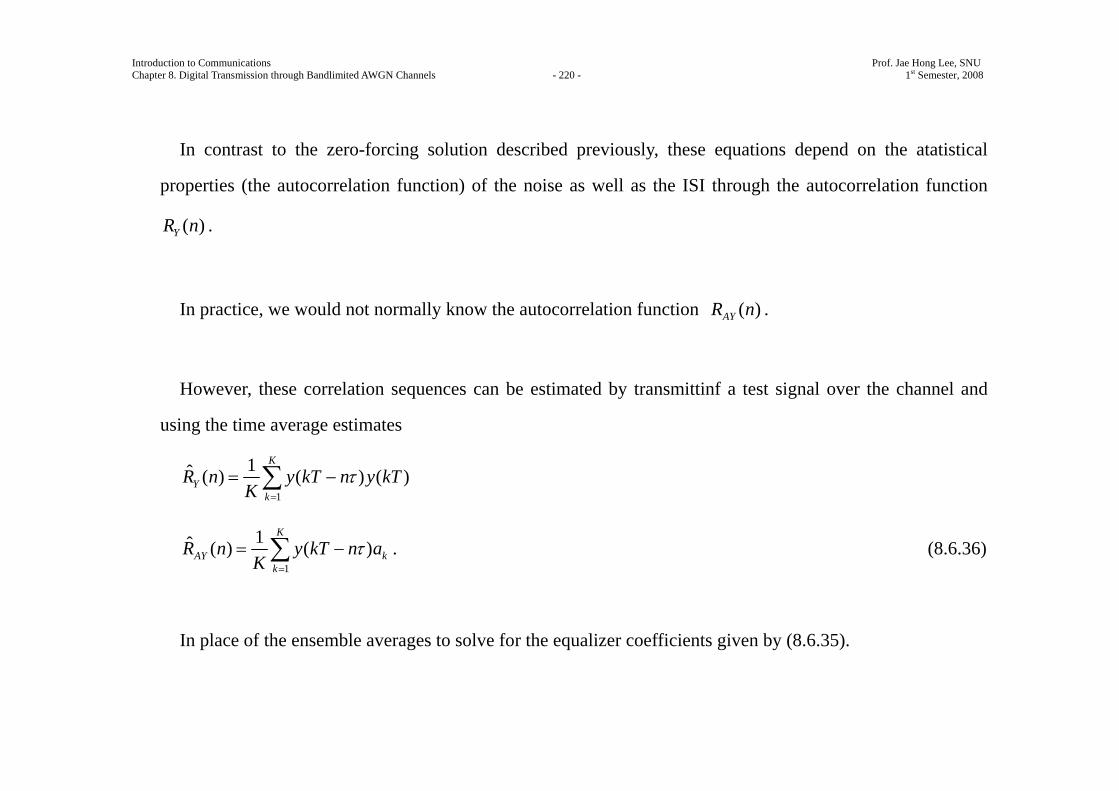
Introduction to Communications Prof. Jae Hong Lee, SNU Chapter 8. Digital Transmission through Bandlimited AWGN Channels - 220 - 1st Semester, 2008
In contrast to the zero-forcing solution described previously, these equations depend on the atatistical
properties (the autocorrelation function) of the noise as well as the ISI through the autocorrelation function
( )YR n .
In practice, we would not normally know the autocorrelation function ( )AYR n .
However, these correlation sequences can be estimated by transmittinf a test signal over the channel and
using the time average estimates
1
1ˆ ( ) ( ) ( )K
Yk
R n y kT n y kTK
τ=
= −∑
1
1ˆ ( ) ( )K
AY kk
R n y kT n aK
τ=
= −∑ . (8.6.36)
In place of the ensemble averages to solve for the equalizer coefficients given by (8.6.35).
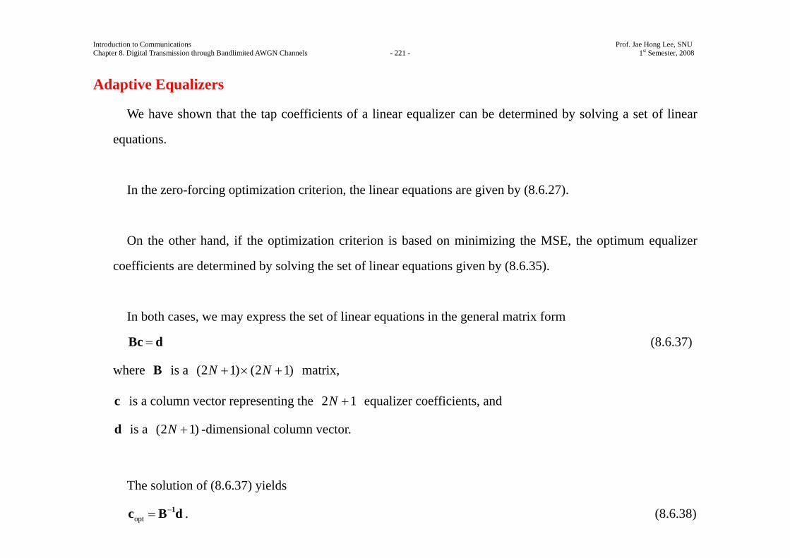
Introduction to Communications Prof. Jae Hong Lee, SNU Chapter 8. Digital Transmission through Bandlimited AWGN Channels - 221 - 1st Semester, 2008
Adaptive Equalizers
We have shown that the tap coefficients of a linear equalizer can be determined by solving a set of linear
equations.
In the zero-forcing optimization criterion, the linear equations are given by (8.6.27).
On the other hand, if the optimization criterion is based on minimizing the MSE, the optimum equalizer
coefficients are determined by solving the set of linear equations given by (8.6.35).
In both cases, we may express the set of linear equations in the general matrix form
=Bc d (8.6.37)
where B is a (2 1) (2 1)N N+ × + matrix,
c is a column vector representing the 2 1N + equalizer coefficients, and
d is a (2 1)N + -dimensional column vector.
The solution of (8.6.37) yields
opt−= 1c B d . (8.6.38)
Introduction to Communications Prof. Jae Hong Lee, SNU Chapter 8. Digital Transmission through Bandlimited AWGN Channels - 222 - 1st Semester, 2008
In practical implementations of equalizers, the solution of (8.6.37) for the optimum coefficient vector is
usually obtained by an iterative procedure that avoids the explicit computation of the inverse of the matrix B .
The simplest iterative procedure is the method of steepest descent, in which one begins by choosing
arbitrarily the coefficient vector c , say 0c .
This initial choice of coefficients corresponds to a point on the criterion function that is begin optimized.
For example, in the case of the MSE criterion, the initial guess 0c corresponds to a point on the quadratic
MSE surface in the (2 1)N + - dimensional space of coefficients.
The gradient vector, defined as 0g , which is the derivative of the MSE with respect to the 2 1N + filter
coefficients, is then computed at this point on the criterion surface and each tap coefficient is changed in the
direction opposite to its corresponding gradient component.
The change in the j th tap coefficient is proportional to the size of the j th gradient component.
Introduction to Communications Prof. Jae Hong Lee, SNU Chapter 8. Digital Transmission through Bandlimited AWGN Channels - 223 - 1st Semester, 2008
For example, the gradient vector, denoted as kg , for the MSE criterion, found by taking the derivatives of
the MSE with respect to each of the 2 1N + coefficients, is given by
, 0,1, 2,k k k= − =g Bc d (8.6.39)
Then the coefficient vector kc is updated according to the relation
1k k k+ = − Δc c g (8.6.40)
where Δ is the step-size parameter for the iterative procedure.
To ensure convergence of the iterative procedure, Δ is chosen to be a small positive number.
In such a case, the gradient vector kg converges toward zero; i.e., k →g 0 as k →∞ , and the coefficient
vector optk →c c as shown in Figure 8.38 based on two-dimensional optimization.
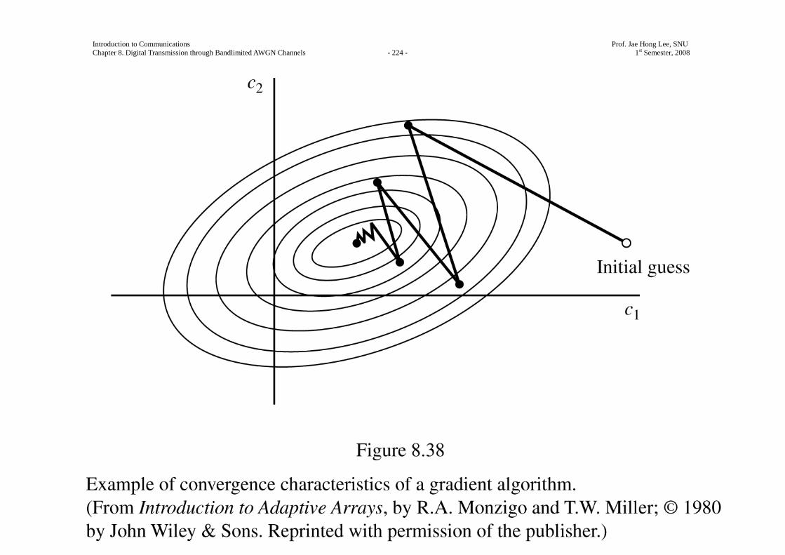
Introduction to Communications Prof. Jae Hong Lee, SNU Chapter 8. Digital Transmission through Bandlimited AWGN Channels - 224 - 1st Semester, 2008

Introduction to Communications Prof. Jae Hong Lee, SNU Chapter 8. Digital Transmission through Bandlimited AWGN Channels - 225 - 1st Semester, 2008
In general, convergence of the equalizer tap coefficients to optc corresponds to a fraction of a second.
Adaptive channel equalization is required for channels whose characteristics change with time. In such a
case, ths ISI varies with time.
The channel equalizer must track such time variations in the channel response and adapt its coefficients to
reduce the ISI.
In the context of the above discussion, the optimum coefficients vector optc varies with time due ti time
variations in the matrix B and, for the case of the MSE criterion, time variations in the vector d .
Under these conditions, the iterative method described above can be modified to use estimates of the
gradient components.
Thus, the algorithm for adjusting the equalizer tap coefficients may be expressed as
1ˆ ˆ ˆk k k+ = − Δc c g (8.6.41)
where ˆ kg denotes an estimate of the gradient vector kg and
Introduction to Communications Prof. Jae Hong Lee, SNU Chapter 8. Digital Transmission through Bandlimited AWGN Channels - 226 - 1st Semester, 2008
ˆkc denotes the estimate of the tap coefficient vector.
In the case of the MSE criterion, the gradient vector kg given by (8.6.39) may also be expressed as (see
Problem 8.46).
)(k k kE e= −g y .
An estimate ˆ kg of the gradient vecrot at the k th iteration is computed as
ˆ k k ke= −g y (8.6.42)
where ke denotes the difference between the desired output from the equalizer at the k th time instant and the
actual output ( )z kT ,
and ky denotes the column vector of 2 1N + received signal values contained in the equalizer at time instant
k .
The error signal ke is expressed as
k k ke a z= − (8.6.43)
Introduction to Communications Prof. Jae Hong Lee, SNU Chapter 8. Digital Transmission through Bandlimited AWGN Channels - 227 - 1st Semester, 2008
where ( )kz z kT= is the equalizer output given by (8.6.32) and ka is the desired symbol.
Hence, by substituting (8.6.42) into (8.6.41), we obtain the adaptive algorithm for optimizing the tap
coefficints (based on the MSE criterion) as
1ˆ ˆk k k ke+ = + Δc c y . (8.6.44)
Since an estimate of the gradient vector is used in (8.6.44) the algorithm is called a stochastic gradient
algorithm or the LMS algorithm.
A block diagram of an adaptive equalizer that adapts its tap coefficients according to (8.6.44) is shown in
Figure 8.39.

Introduction to Communications Prof. Jae Hong Lee, SNU Chapter 8. Digital Transmission through Bandlimited AWGN Channels - 228 - 1st Semester, 2008
Introduction to Communications Prof. Jae Hong Lee, SNU Chapter 8. Digital Transmission through Bandlimited AWGN Channels - 229 - 1st Semester, 2008
Note that the difference between the desired output ka and the actual output kz from the equalizer is used
to form the error signal ke multiplies the received signal values { ( )}y kT nτ− at the 2 1N + taps.
The products ( )ke y kT nτΔ − at the (2 1)N + taps are then added to the previous values of the tap
coefficients to obtain the updated tap coefficients, according to (8.6.44).
This computation is repeated for each received symbol.
Thus, the equalizer coefficients are updated at the symbol rate.
Initially, the adaptive equalizer is trained by the transmission of a known pseudo-random sequence { }ma
over the channel.
At the demodulator, the equalizer employs the known sequence to adjust its coefficients.
Upon initial adjustment, the adaptive equalizer switches from a traning mode to a decision-directed mode,
in which case the decisions at the output of the detector are sufficiently reliable so that the error signal is
Introduction to Communications Prof. Jae Hong Lee, SNU Chapter 8. Digital Transmission through Bandlimited AWGN Channels - 230 - 1st Semester, 2008
formed by computing the difference between the detector output and the equalizer output; i.e.,
k k ke a z= − (8.6.45)
where ka is the output of the detector.
In general, decision erroes at the output of the detector occur infrequently and, consequently, such errors
have little effect on the performance of the tracking algorithm given by (8.6.44).
A rule of thumb for selecting the step-size parameter so as to ensure convergence and good tracking
capabilities in slowly varying channel is given by
15(2 1) RN P
Δ =+
(8.6.46)
where RP denotes the received signal-plus-noise power, which can be estimated from the received signal.
The convergence characteristics of the stochastic gradient algorithm in (8.6.44) is shown in Figure 8.40.
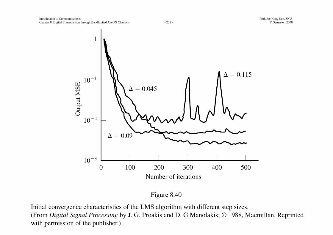
Introduction to Communications Prof. Jae Hong Lee, SNU Chapter 8. Digital Transmission through Bandlimited AWGN Channels - 231 - 1st Semester, 2008
Introduction to Communications Prof. Jae Hong Lee, SNU Chapter 8. Digital Transmission through Bandlimited AWGN Channels - 232 - 1st Semester, 2008
These graphs were obtained from a computer simulation of an 11-tap adaptive equalizer operating a
channel with a rather modest amount of ISI.
The input signal-plus-noise power RP was normalized to unity.
The rule of thumb given in (8.6.46) for selecting the step size gives 0.018Δ = .
The effect of making Δ too large is illustrated by the large jumps in MSE as shown for 0.115Δ = .
As Δ is decreased, the convergence is slowed somewhat, but a lower MSE is achieved, indicating that the
estimated coefficients are closer to optc .
Although we have described in some detail the operation of an adaptive equalizer which is optimized on the
basis of the MSE criterion, the operation of an adaptive equalizer based on the zero-forcing method is very
similar.
The major difference lies in the method for estimating the gradient vectors kg at each iteration.

Introduction to Communications Prof. Jae Hong Lee, SNU Chapter 8. Digital Transmission through Bandlimited AWGN Channels - 233 - 1st Semester, 2008
A block diagram of an adaptive zero-forcing equalizer is shown in Figure 8.41.
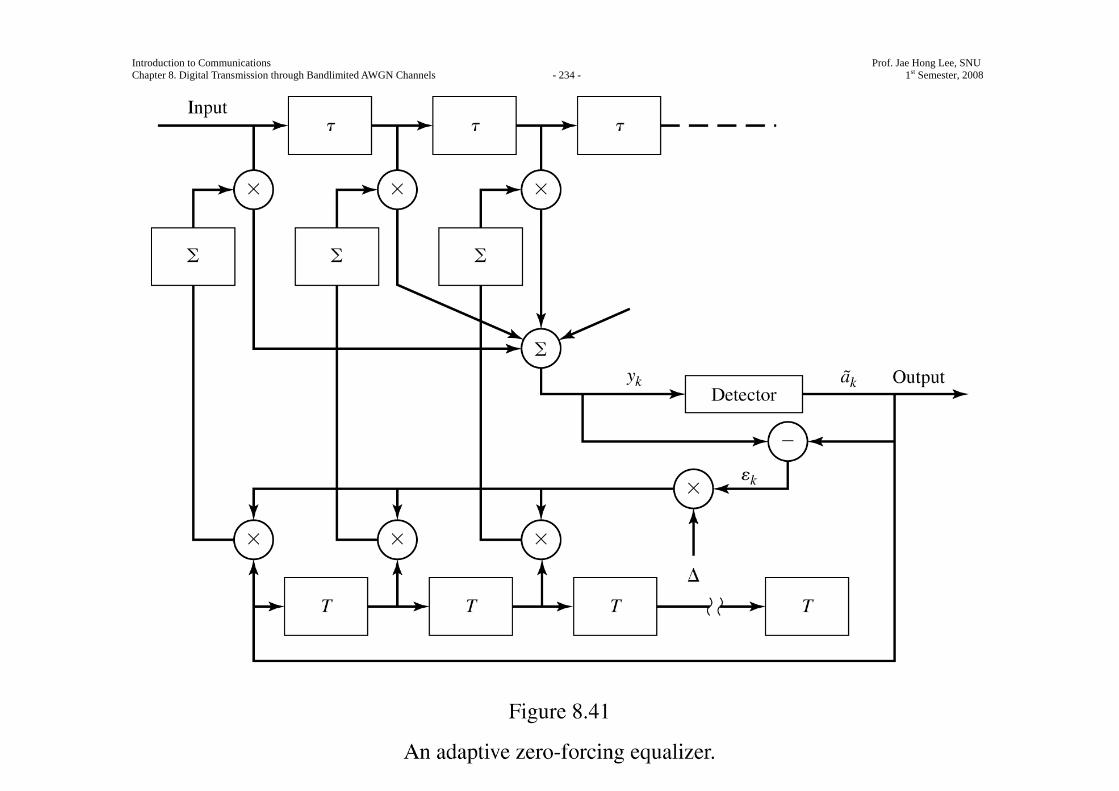
Introduction to Communications Prof. Jae Hong Lee, SNU Chapter 8. Digital Transmission through Bandlimited AWGN Channels - 234 - 1st Semester, 2008
Introduction to Communications Prof. Jae Hong Lee, SNU Chapter 8. Digital Transmission through Bandlimited AWGN Channels - 235 - 1st Semester, 2008
Decision-Feedback Equalizer
The linear filter equalizers described above are very effective on channels, such as wireline telephone
channels, where the ISI is not severe.
The severity of the ISI is directly related to the spectral characteristics and not necessarily to the time span
of the ISI.
For example, consider the ISI resulting from two channels which are shown in Figure 8.42.
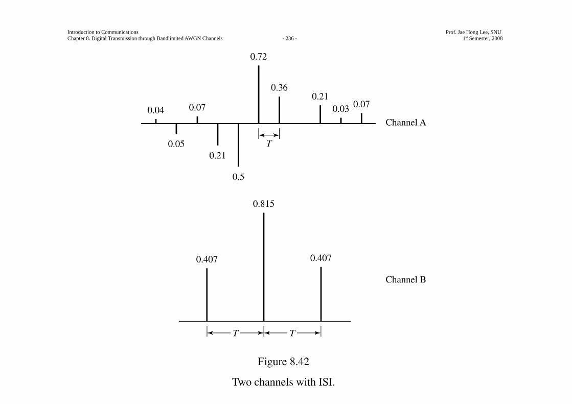
Introduction to Communications Prof. Jae Hong Lee, SNU Chapter 8. Digital Transmission through Bandlimited AWGN Channels - 236 - 1st Semester, 2008
Introduction to Communications Prof. Jae Hong Lee, SNU Chapter 8. Digital Transmission through Bandlimited AWGN Channels - 237 - 1st Semester, 2008
The time span for the ISI in Channel A is 5 symbol intervals on each side of the desired signal
component, which has a value of 0.72 .
On the other hand, the time span for the ISI in Channel B is one symbol interval on each side of the
desired signal component, which has a value of 0.815 .
The energy of the total response is normalized to unity for both channels.
In spite of the shorter ISI span, Channel B results in more severe ISI.
This is evidenced in the frequency response characteristics of these channels, which are shown in Figure
8.43.
We observe that Channel B has a spectral null (the frequency response characteristics of these channels,
which are shown in Figure 8.43.

Introduction to Communications Prof. Jae Hong Lee, SNU Chapter 8. Digital Transmission through Bandlimited AWGN Channels - 238 - 1st Semester, 2008
Introduction to Communications Prof. Jae Hong Lee, SNU Chapter 8. Digital Transmission through Bandlimited AWGN Channels - 239 - 1st Semester, 2008
We observe that Channel B has a spectral null (the frequency response ( ) 0C f = for some frequencies in
the band | |f W≤ ) at 12
fT
= , whereas this does not occur in the case of Channel A .
Consequently, a linear equalizer will introduce a large gain in its frequency response to compensate for the
channel null.
Thus, the noise in Channel B will be enhanced much more than in Channel A .
This fact is borne out by the computer simulation results for the performance of the linear equalizer for the
two channels, as shown in Figure 8.44.
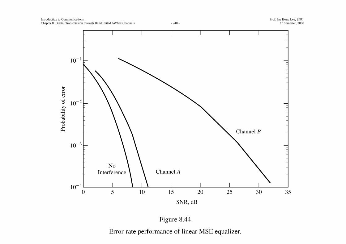
Introduction to Communications Prof. Jae Hong Lee, SNU Chapter 8. Digital Transmission through Bandlimited AWGN Channels - 240 - 1st Semester, 2008
Introduction to Communications Prof. Jae Hong Lee, SNU Chapter 8. Digital Transmission through Bandlimited AWGN Channels - 241 - 1st Semester, 2008
Hence, the basic limitation of a linear equalizer is that it performs poorly on channels having spectral nulls.
Such channels are often encountered in radio channels, such as those used for cellular radio
communications.
A decision-feedback equalizer (DFE) is a nonlinear equalizer that employs previous decision to eliminate
the ISI caused by previously detected symbols on the current symbol to be detected.
A simple block diagram for a DFE is shown in Figure 8.45.
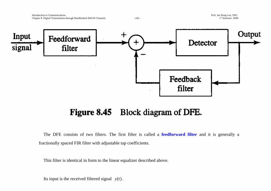
Introduction to Communications Prof. Jae Hong Lee, SNU Chapter 8. Digital Transmission through Bandlimited AWGN Channels - 242 - 1st Semester, 2008
The DFE consists of two filters. The first filter is called a feedforward filter and it is generally a
fractionally spaced FIR filter with adjustable tap coefficients.
This filter is identical in form to the linear equalizer described above.
Its input is the received filtered signal ( )y t .
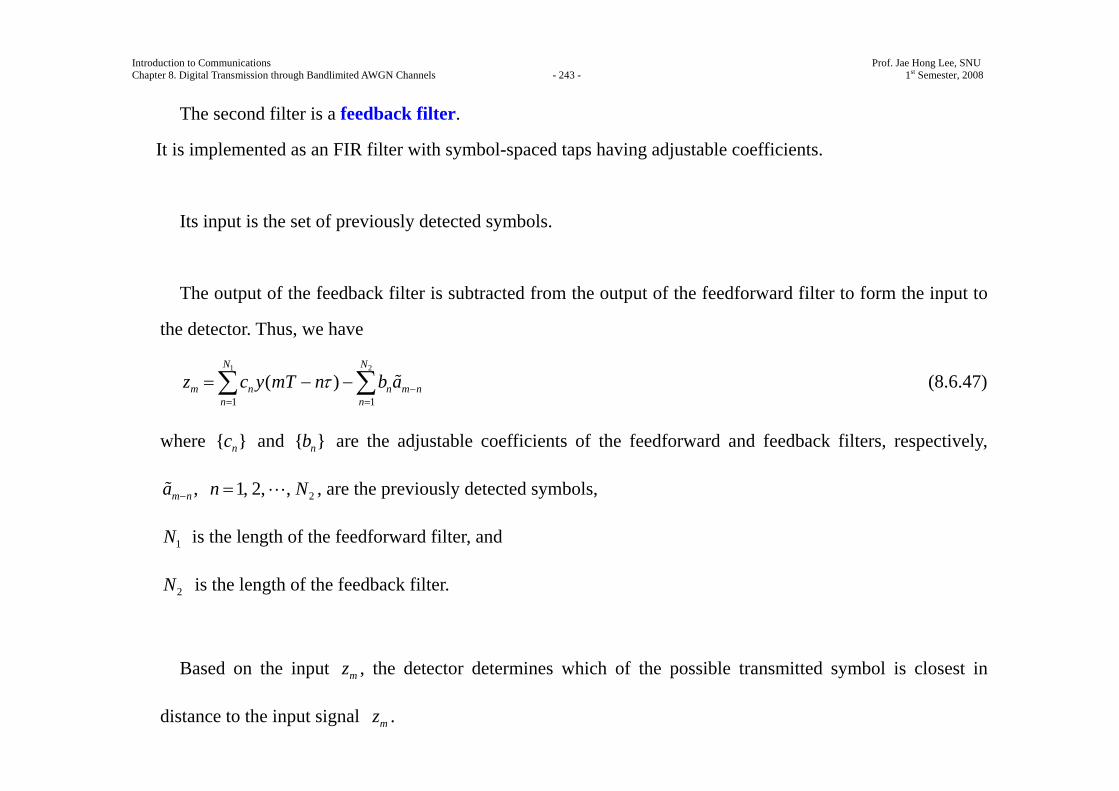
Introduction to Communications Prof. Jae Hong Lee, SNU Chapter 8. Digital Transmission through Bandlimited AWGN Channels - 243 - 1st Semester, 2008
The second filter is a feedback filter.
It is implemented as an FIR filter with symbol-spaced taps having adjustable coefficients.
Its input is the set of previously detected symbols.
The output of the feedback filter is subtracted from the output of the feedforward filter to form the input to
the detector. Thus, we have
1 2
1 1
( )N N
m n n m nn n
z c y mT n b aτ −= =
= − −∑ ∑ (8.6.47)
where { }nc and { }nb are the adjustable coefficients of the feedforward and feedback filters, respectively,
2, 1, 2, ,m na n N− = , are the previously detected symbols,
1N is the length of the feedforward filter, and
2N is the length of the feedback filter.
Based on the input mz , the detector determines which of the possible transmitted symbol is closest in
distance to the input signal mz .
Introduction to Communications Prof. Jae Hong Lee, SNU Chapter 8. Digital Transmission through Bandlimited AWGN Channels - 244 - 1st Semester, 2008
Thus, it makes its decision and output ma .
What makes the DFE nonlinear is the nonlinear characteristic of the detector which provides the input to the
feedback filter.
The tap coefficient of the feedforward and feedback filters are selected to optimize some desired
performance measure.
For mathematical simplicity, the MSE criterion is usually applied and a stochastic gradient algorithm is
commonly used to implement an adaptive DFE.
Figure 8.46 shows the block diagram of an adaptive DFE whose tap coefficients are adjusted by means of
the LMS stochastic gradient algorithm.
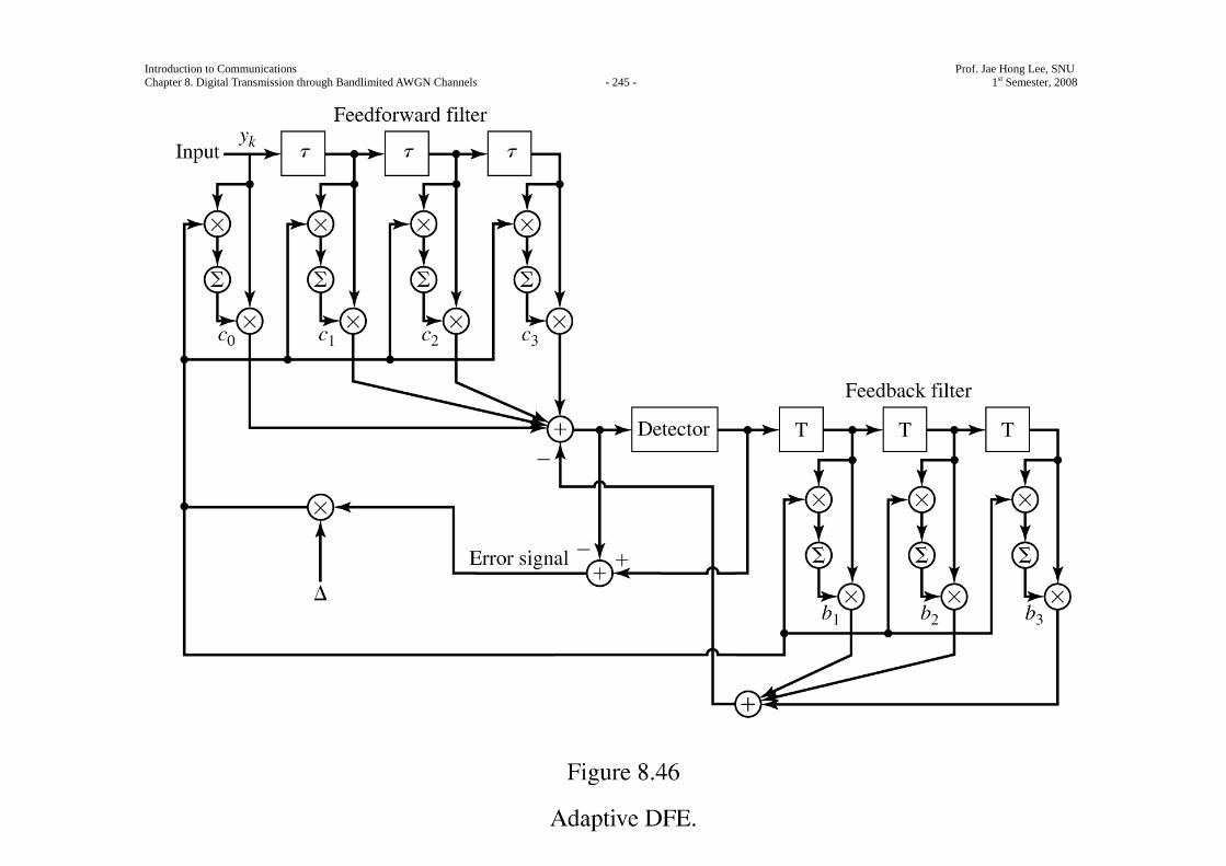
Introduction to Communications Prof. Jae Hong Lee, SNU Chapter 8. Digital Transmission through Bandlimited AWGN Channels - 245 - 1st Semester, 2008
Introduction to Communications Prof. Jae Hong Lee, SNU Chapter 8. Digital Transmission through Bandlimited AWGN Channels - 246 - 1st Semester, 2008
Figure 8.47 shows the probability of error performance of the DFE, obtained by computer simulation, for
binary PAM transmission over Channel B.
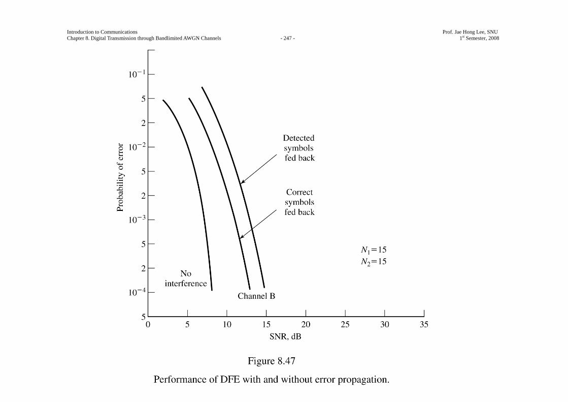
Introduction to Communications Prof. Jae Hong Lee, SNU Chapter 8. Digital Transmission through Bandlimited AWGN Channels - 247 - 1st Semester, 2008
Introduction to Communications Prof. Jae Hong Lee, SNU Chapter 8. Digital Transmission through Bandlimited AWGN Channels - 248 - 1st Semester, 2008
The gain in performance relative to that of a linear equalizer is clearly evident.
We should mention that decision errors from the detector that are fed to the feedback filter have a small
effect on the performance of the DFE.
In general, a small loss in performance of one to two dB is possible at error rates below 210− , but the
decision errors in the feedback filters are not catastrophic.
Although the DFE outperforms a linear equalizer, it is not the optimum equalizer freom the viewpoint of
minimizing the probability of error.
As indicated previously equalizer from the optimum detector in a digital communication system in the
presence of ISI is a ML symbol sequence detector.
It is particularly appropriate for channels with severe ISI, when the ISI spans only a few signals.
For example Figure 8.48 shows the error probability performance of the Viterbi algorithm for binary PAM
signal transmitted through channel B (see Figure 8.42).
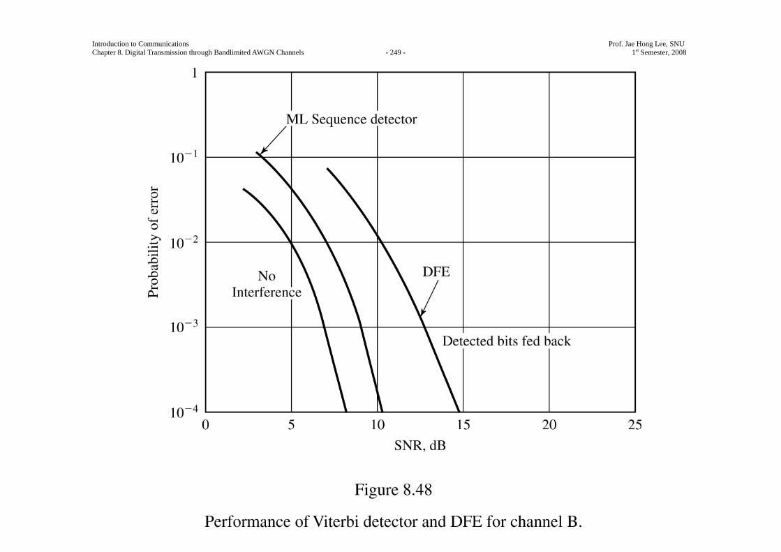
Introduction to Communications Prof. Jae Hong Lee, SNU Chapter 8. Digital Transmission through Bandlimited AWGN Channels - 249 - 1st Semester, 2008
Introduction to Communications Prof. Jae Hong Lee, SNU Chapter 8. Digital Transmission through Bandlimited AWGN Channels - 250 - 1st Semester, 2008
For purposes of comparison, we also illustrate the probability of error for a decision feedback equalizer.
Both results were obtained by computer simulation.
We observe that the performance of the ML sequence detector is about 4.5 -dB better than that of the DFE
at an error probability of 410− .
Hence, this is one example where the ML sequence detector provides a significant performance gain on a
channel which has a relatively short ISI span.
In conclusion, we mention that adaptive equalizers are widely used in high-speed digital communication
systems for telephone channels.
High-speed telephone line modems (bit rate above 2400 bps) generally include an adaptive equalizer that
is implemented as an FIR filter with coefficients that are adjusted based on the MMSE criterion.
Depending on the data speed, the equalizer typically soans between 20 and 70 symbols.
Introduction to Communications Prof. Jae Hong Lee, SNU Chapter 8. Digital Transmission through Bandlimited AWGN Channels - 251 - 1st Semester, 2008
The LMS algjrithm given by (8.6.44) is usually employed for the adjustment of the equalizer coefficients
adaptively.
Introduction to Communications Prof. Jae Hong Lee, SNU Chapter 8. Digital Transmission through Bandlimited AWGN Channels - 252 - 1st Semester, 2008
8.7 Multicarrier Modulation And OFDM
We observed that inter-symbol interference results in performance degradation, even when the optimum
detector is used to recover the information symbols at the receiver.
An alternative approach to designing a bandwidth-efficient communication system in the presence of
channel distortion is to subdivide the available channel bandwidth into a number of equal-bandwidth
subchannels each of which bandwidth is sufficiently narrow so that the frequency response of the subchannels
are nearly ideal.
Such a subdivision of the overall bandwidth into smaller subchannels with bandwidth fΔ is shown in
Figure 8.49.
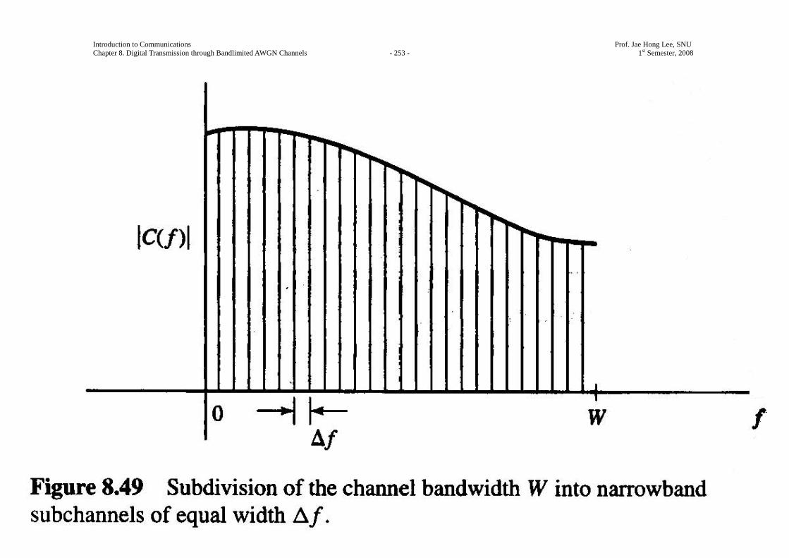
Introduction to Communications Prof. Jae Hong Lee, SNU Chapter 8. Digital Transmission through Bandlimited AWGN Channels - 253 - 1st Semester, 2008
Introduction to Communications Prof. Jae Hong Lee, SNU Chapter 8. Digital Transmission through Bandlimited AWGN Channels - 254 - 1st Semester, 2008
Then, different information symbols are transmitted simultaneously through WKf
=Δ
subchannels.
Consequently, the data is transmitted by frequency-division multiplexing (FDM).
With each subchannel, we associate a carrier signal given by
( ) sin 2 , 0,1, , 1k kx t f t k Kπ= = − , (8.7.1)
where kf is the mid-frequency of the k th subchannel.
By selecting the symbol rate 1T
on each of the subchannels to be equal to the separation fΔ between
adjacent subcarriers, the subcarriers become orthogonal over the symbol interval T , independent of the
relative phase relationship between subcarriers.
That is,
0sin(2 )sin(2 ) 0
T
k k j jf t f t dtπ φ π φ+ + =∫ (8.7.2)
where , 1, 2, ,k jnf f nT
− = = independent of the phase kφ and jφ .
Introduction to Communications Prof. Jae Hong Lee, SNU Chapter 8. Digital Transmission through Bandlimited AWGN Channels - 255 - 1st Semester, 2008
In this case, we have orthogonal frequency-division multiplexing (OFDM).
With an OFDM system having K subchannels, the symbol rate on each subcarrier is reduced by a factor
of K relative to the symbol rate on a single carrier system which employs the entire bandwidth W to
transmit data at the same rate as OFDM.
Hence, the symbol interval in the OFDM system is ST KT= , where ST is the symbol interval in the
single-carrier system.
By selecting K to be sufficiently large, the symbol interval T can be made significantly larger than the
duration of time dispersion of the channel.
Thus, intersymbol interference can be made arbitrarily small by the selection of K .
In other words, each subchannel appears to have a fixed frequency response ( ), 0,1, , 1kC f k K= − .
Introduction to Communications Prof. Jae Hong Lee, SNU Chapter 8. Digital Transmission through Bandlimited AWGN Channels - 256 - 1st Semester, 2008
As long as we maintain time synchronization among the subcarriers, OFDM allows us to transmit a
different number of bits/symbol on each subcarrier.
Hence, subcarriers which yield a higher SNR due to a lower attenuation can be modulated by a higher level
modulation scheme (with more bits/symbol) than subchannels which yield a lower SNR (due to higher
attenuation).
For example, QAM with various constellation sizes may be used in an OFDM system.
The modulator and demodulator in an OFDM system can be implemented by use of a parallel bank of filters
based on the diecrete Fourier transform (DFT).
When the number of subchannels is large, say 25K > , the modulator and demodulator in an OFDM system
are efficiently implemented by using the fast Fourier transform algorithm (FFT) to compute the DFT.
Next, we describe an OFDM system in which the modulator and demodulator are implemented based on the
DFT.
Introduction to Communications Prof. Jae Hong Lee, SNU Chapter 8. Digital Transmission through Bandlimited AWGN Channels - 257 - 1st Semester, 2008
A major problem with the multicarrier modulation in general and OFDM system in particular is the high
peak-to-average power ratio (PAR) that is inherent in the transmitted signal.
Large signal peaks occur in the transmitted signal when the signals in the K subchannels add
constructively in phase.
Such large signal peaks may saturate the power amplifier at the transmitter to cause intermodulation
distortion in the transmitted signal.
Intermodulation distortion can be reduced and avoided by reducing the average power of the transmitted
signal to make the power amplifier to operate in the linear range.
Such power reduction results in inefficient operation of the OFDM system.
A variety of methods have been devised to reduce PAR in multicarrier systems.
A relatively simple method is to insert different phase shifts in each of the subcarriers, where the phase
shifts are selected pseudorandomly, or by means of some algorithm, to reduce the PAR.
Introduction to Communications Prof. Jae Hong Lee, SNU Chapter 8. Digital Transmission through Bandlimited AWGN Channels - 258 - 1st Semester, 2008
8.7.1 An OFDM System Implemented via the FFT Algorithm
The basic block diagram of the OFDM is shown in Figure 8.50.
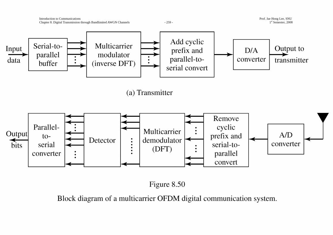
Introduction to Communications Prof. Jae Hong Lee, SNU Chapter 8. Digital Transmission through Bandlimited AWGN Channels - 259 - 1st Semester, 2008
Introduction to Communications Prof. Jae Hong Lee, SNU Chapter 8. Digital Transmission through Bandlimited AWGN Channels - 260 - 1st Semester, 2008
A serial-to-parallel buffer subdivides the information sequence into frames of fB bits.
The fB bits in each frame are parsed into K groups, where the i th group is assigned ib bits.
Hence,
1
K
i fi
b B=
=∑ . (8.7.3)
We may view the multicarrier modulator as generating K independent QAM subchannels,
where the symbol rate for each subchannel is 1T
and
the signal in each subchannel has a distinct QAM constellation.
Hence, the number of signal points in the constellation for the i th subchannel is 2 ibiM = .
Let kX , 0,1, , 1k K= − , denote the complex-valued signal points corresponding to the information
signals on the K subchannels.

Introduction to Communications Prof. Jae Hong Lee, SNU Chapter 8. Digital Transmission through Bandlimited AWGN Channels - 261 - 1st Semester, 2008
These information symbols { }kX represent the values of the discrerte Fourier transform (DFT) of a
multicarrier OFDM signal ( )x t , where the modulation on each subcarrier is QAM.
Since ( )x t must be a real-valued signal, its N -point DFT { }kX must satisfy the symmetry property
N k kX X ∗− = .
Therefore, we create 2N K= symbols from K information symbols by defining
, 1, 2, , 1N k kX X k K∗− = = − , (8.7.4)
'0 0Re( )X X= (8.7.5)
0Im( )NX X= . (8.7.6)
Note that the information symbol 0X is split into two parts, both of which are real.
If we denote the new sequence of symbols as '{ , 0,1, , 1}kX k N= − , the N -point inverse DFT (IDFT)
Introduction to Communications Prof. Jae Hong Lee, SNU Chapter 8. Digital Transmission through Bandlimited AWGN Channels - 262 - 1st Semester, 2008
yields the real-valued sequence
21'
0
1 nkN jN
n kk
x X eN
π−
=
= ∑ , 0,1, , 1n N= − . (8.7.7)
where 1N
is simply a scale factor.
This sequence { , 0 1}nx n N≤ ≤ − corresponds to samples of the multicarrier OFDM signal ( )x t ,
consisting of K subcarriers, which may be expressed as
21'
0
1( ) , 0ktN j
Tk
kx t X e t T
N
π−
=
= ≤ ≤∑ , (8.7.8)
where T is the signal duration and ( ), 0,1, , 1nnTx x n NN
= = − .
The signal samples { }nx generated by computing the IDFT are passed through a digital-to-analog (D/A)
converter, where output, ideally is the OFDM signal waveform ( )x t .
With ( )x t as the input to the channel, the channel output at the receiver may be expressed as
Introduction to Communications Prof. Jae Hong Lee, SNU Chapter 8. Digital Transmission through Bandlimited AWGN Channels - 263 - 1st Semester, 2008
( ) ( ) ( ) ( )r t x t c t n t= ∗ + (8.7.9)
where ( )c t is the impulse response of the channel and ∗ stands for convolution.
Since the bandwidth fΔ of each subchannel is selected to be very small relative to the overall channel
bandwidth W K f= Δ , the symbol duration 1Tf
=Δ
is large compared to the duration of the channel impulse
response.
To be specific, suppose that the channel impulse response spans 1m + signal samples, where m N<< .
A simple way to completely avoid intersymbol interference (ISI) is to insert a time guard of duration mTN
between transmission of successive data blocks.
This allows the response of the channel to die out before the next block of K symbols are transmitted.
An alternative method to avoid ISI is to append a so-called cyclic prefix to each block of N signal
samples { , 0 1}nx n N≤ ≤ − .
Introduction to Communications Prof. Jae Hong Lee, SNU Chapter 8. Digital Transmission through Bandlimited AWGN Channels - 264 - 1st Semester, 2008
The cyclic prefix for the block of samples consists of the samples 1 1, , ,N m N m Nx x x− − + − .
These samples are appended to the beginning of the block, thus, creating a signal sequence of length
N m+ samples, which may be indexed from n m= − to 1n N= − , where the first m samples constitute
the cyclic prefix.
Then, if the sample values of the channel response are { , 0 }nc n m≤ ≤ , the convolution of { }nc with
{ , 1}nx m n N− ≤ ≤ − produce the received signal { }nr .
Since the ISI in any pair of successive signal transmission blocks affects the first m signal samples, we
discard the first m samples of { }nr and demodulate the signal based on the received signal samples
{ , 0 1}nr n N≤ ≤ − .
If we view the channel characteristics in the frequency domain, the channel frequency response at the
subcarrier frequencies kkfT
= is given by
Introduction to Communications Prof. Jae Hong Lee, SNU Chapter 8. Digital Transmission through Bandlimited AWGN Channels - 265 - 1st Semester, 2008
2k
kC CNπ⎛ ⎞= ⎜ ⎟
⎝ ⎠
2 /
0
, 0,1, , 1m
j nk Nn
n
c e k Nπ−
=
= = −∑ . (8.7.10)
Since the ISI is eliminated by the use of either the cyclic prefix or the time quard band, the demodulated
sequence of symbols may be expressed as
'ˆ , 0,1, , 1k k k kX C X k Nη= + = − , (8.7.11)
where ˆ{ }kX is the output of the N -point DFT computed by the demodulator and
{ }kη is the additive noise corrupting the signal.
As shown in Figure 8.50, the received signal is demodulated by computing the DFT of the received signal
after it has been passed through an analog-to-digital (A/D) converter.
As in the case of the OFDM modulator, the DFT computation at the demodulator is performed efficiently by
use of the FFT algorithm.
Introduction to Communications Prof. Jae Hong Lee, SNU Chapter 8. Digital Transmission through Bandlimited AWGN Channels - 266 - 1st Semester, 2008
In order to recover the information symbols from the values of the computed DFT, it is necessary to
estimate and compensate for the channel factors { }kC .
The channel measurement can be accomplished by initially transmitting either a known modulated sequence
on each of the subcarriers or, simply, transmitting the unmodulated subcarriers.
If the channel characteristics vary slowly with time, the time variations can be tracked by using the
decisions at the output of the detector in a decision-directed manner.
Thus, the multicarrier OFDM system can be made to operate adaptively.
The transmission rate on each of the subcarriers can be optimized by properly allocating the average
transmitted power and the number of bits that are transmitted by each subcarrier.
The SNR per subchannel may be defined as
2
2
| |SNR k kk
nk
TP Cσ
= (8.7.12)
where T is the symbol duration,
Introduction to Communications Prof. Jae Hong Lee, SNU Chapter 8. Digital Transmission through Bandlimited AWGN Channels - 267 - 1st Semester, 2008
kP is the average transmitted power allocated to the k th subchannel,
2| |kC is the squared magnitude of the frequency response of the k th subchannel, and
2nkσ is the corresponding noise variance.
In subchannels with high SNR, we transmit more bits/symbol by using a larger QAM constellation
compared to subchannels with low SNR.
Thus, the bit rate on each subchannel can be optimized in such a way that the error-rate performance among
the subchannels is equalized to satisfy the desired specifications.
Multicarrier OFDM using QAM modulation on each of the subcarriers as described above has been
implemented for a variety of applications, including high-speed transmission over telephone lines, such as
digital subcarrier lines.
This type of multicarrier OFDM modulation has also been called discrete-multitone (DMT) modulation.
Multicarrier OFDM is also used in digital audio broadcasting in Europe and other parts of the world and in
Introduction to Communications Prof. Jae Hong Lee, SNU Chapter 8. Digital Transmission through Bandlimited AWGN Channels - 268 - 1st Semester, 2008
digital celluar communication systems.