CHAPTER 7 TREND AND PATTERN OF MONEY

AND REAL WAGES IN KERALA

Trend and pattern of money wages and real wages in Kerala

Studies on wage earnings of labourers in the agricultural sector assume

special significance on account of the irregular and erratic nature of

employment compounded further by total or near total absence of alternative

sources of employment and income. The associations between available days

of employment and agricultural wage income of labourers on the one side and

rural poverty on the other have sufficiently been explored and statistically

established in the Indian context1• The objective of the chapter is to analyse the

trend in the money, real and product wages of different categories of labourers

in Kerala over the years and also to identify the major determinants of the daily

wage earnings of labourers, using a supply-demand framework. The supply­

demand framework is employed to examine the extent to which the observed

differences in wage rates can be explained. The analysis in the chapter is based

on secondary source of information on wages and other variables. Given the

setting, the chapter is organized into three sections. The first section of the

chapter examines different sources of wage data for agricultural labourers and

also discusses issues in the source of wage data used for the present study. In

the second section, the trend in money and real wage rates of different types of

labourers in the rural sector by districts in the state over a period of 47 years is

analysed in the background of the findings of various studies on the trend in

rate of growth in real wages of the state vis-a-vis other states and national

average. Important factors influencing the wage rate are identified by

1 Sundaram, K. (200 I). Employment and poverty in the 1990s: Further results from NSS 55'h round on employment unemployment survey, 1999-2000. Economic and political weekly. XXXVI (32): 3039-49. Sundaram, K and Tendulkar, S. (2003). Poverty in India in the 1990s: Revised estimates. Economic and political weekly, XXXVIII (46): 4865-4872. Deaton, A. and Dreze, J. (2002). Poverty and inequality in India: A re-examination. Economic and political weekly, XXXVII (36): 3729-48. Panchamukhi, V. R. (2002). Social impact of economic reforms in India: A critical appraisal. Economic and political weekly, XXXV (10): 836.

197

constructing an econometric mo<!el of wage determination in the third section

of the chapter followed by a subsection on the broad conclusions that emerge

Section 1

7.1. Sources ofwage data for rural labour households

7.1.1. Important sources ofwage data.

Wage data for different categories of labourers in the rural sector are

collected, compiled and published by three national level agencies, viz.,

Ministry of Agriculture (MoA), National Sample Survey Organisation (NSSO)

and Indian Labour Bureau ILB). Even though there are only three agencies

involved in the compilation and publication of wage data, five different

estimates are available on the wage rates in India:

I. Agricultural Wages in India (A WI)- Ministry of Agriculture

2. Agricultural wages from cost of cultivation survey- Ministry of

Agriculture

3. Rural Labour Enquiry Report- Labour Bureau and NSSO

4. Wage Rates in Rural India- Labour Bureau and NSSO

5. NSS Wage data- NSSO

The quniquennial survey conducted by the National Sample Survey

Organisation on behalf of the Labour Bureau for its Rural Labour Enquiry

Report is an important source of wage data for agricultural labour households

in India. Rural Labour Enquiry was conducted for the first time in 1950-51.

The first two rounds of the surveys were confined to agricultural labour

households and the coverage was extended to include all rural labour

households from its third round in 1963-65. Until 1999-00, eight Agricultural!

Rural Labour Enquiries were conducted. Agricultural Labour Enquiry Report

and Rural Labour Enquiry Commission's reports, taken together, \vould supply

data for eight years on a quinquennial basis; 1950-51, 1956-57, 1963-65, 1974-

75, 1977-78, 1983, 1987-88, 1993-94 and 1999-2000. Since 1977-78. the data

collection for Rural Labour Enquiries has been integrated with the general

198

employment and unemployment survey of the NSSO. In addition to the

information furnished on wages and earning by sex and social groupings, RLE

collects and publishes data on consumer expenditure and employment and

unemployment of rural and agricultural labourers too. However, a major

limitation of RLE data particularly from the point of view of the present study

is that the district wise wage statistics for different categories of labourers by

agricultural operations are not being furnished.

Data collected by NSSO on behalf of RLE are published by NSSO.

Even though the sampling frame and methodology of data collection remain

the same for RLE and NSSO, differences between RLE and NSSO reports of

the wage rate are noted on account of the differences in the methodology of

estimation procedure2• The basic conceptual difference in the estimation of

wage data is that RLE classifies rural labour households based on their income

source such as self employed, salary earners and other non-productive sources

(interest and rents). On the contrary, NSSO supplies data based on activity

status of the person, viz., regular or salaried worker and casual workers in

public works and causal workers in private works. For all practical purposes,

\Vage data collected by NSSO-RLE are considered to be superior to the wage

data compiled by the Ministry of Agriculture and published in Agricultural

wages in India and Agricultural Situation in India.

Another important wage data series was released jointly by NSSO and

Indian Labour Bureau in 1986-87. For the revision of consumer price index for

agricultural labourers, retail prices and wage data are collected from the same

sample, which places the date source superior in quality to others. Under the

series, wage data for eleven agricultural and seven non-agricultural

occupations have been collected on a monthly basis since 1986-87. Data

collection under the scheme covers 600 sample villages and 66 NSSO regions

of20 states. Even though the data are collected by NSSO, Labour Bureau does

compilation and publication and the series is published every month in the

1

- Himanushu, (2005). Wages in rural India: Sources, trends and comparability. The Indian of Journal Labour Economics, 48(2): 375-406.

199

Indian Labour Journal since 19983• Notwithstanding the superiority ofthe data,

the data is collected using the same staff and administrative machinery, which

collects information for A WI and, therefore, suffers from the same set of

constraints as A WI. Moreover, it is reported to have gaps with respect to many

occupations and also the aggregate figures at the district and state levels are

arrived at by simple averages4.

As part of the estimation of cost of cultivation, Agricultural

Universities in states collect wage data for 27 crops. The source covers 9000

households spread all over India and such cost of cultivation data is available

from 1971. Like any other source of wage data, Cost of Cultivation Scheme

too suffers from certain limitations which originate mostly from the fact that

the data have been collected as part of the cost of cultivation survey and is not

in a proper format to be readily used as in the case of data from other sources5.

7.1.2. Agricultural wages in India

Among the above mentioned five sources of estimates on agricultural

wages, A WI is the oldest and perhaps the most widely used source of data by

researchers as well as policy makers. A unique advantage of the wage data

published in A WI and Agricultural Situation in India that wage statistics at the

district level (centre-\vise) are available only from A WI (Agricultural situation

in India too supplies information at the district level). It may be noted that the

NSSO data do not provide district-wise wage statistics. District-wise wage

rates for agricultural labourers assume significance in the context of the

observed significant differences in wage levels for the same type of labourers

across districts within a state. On behalf of the Ministry of Agriculture, the

Department of Economics and Statistics of every state government in India

collects information from selected centres in all districts on agricultural wages.

However, wage data published in A WI face the following limitations: i).

Wage data are collected by non-trained and inexperienced government officials

3 Ibid. ~Ibid. ; Ibid.

200

at the local level and the data collection is not based on any scientific and

systematic sampling procedure as adopted by NSS06; ii) More than a decade

has been taken to include newly formed districts into the list of wage collection

centers of A WI. Further, on bifurcation of old districts, wage collection centres

of the bifurcated districts would then be located in the newly formed district.

but wage rate elicited from the same centre was reported for the old district.

Such problems arise on account of the absence of periodical reviewing of

centers based on district delimitation. For example, there are 13 centres from

which wage data for agricultural labourers are reported in A WI for Kerala.

These centres correspond to I 0 districts in the state, but the state has 14

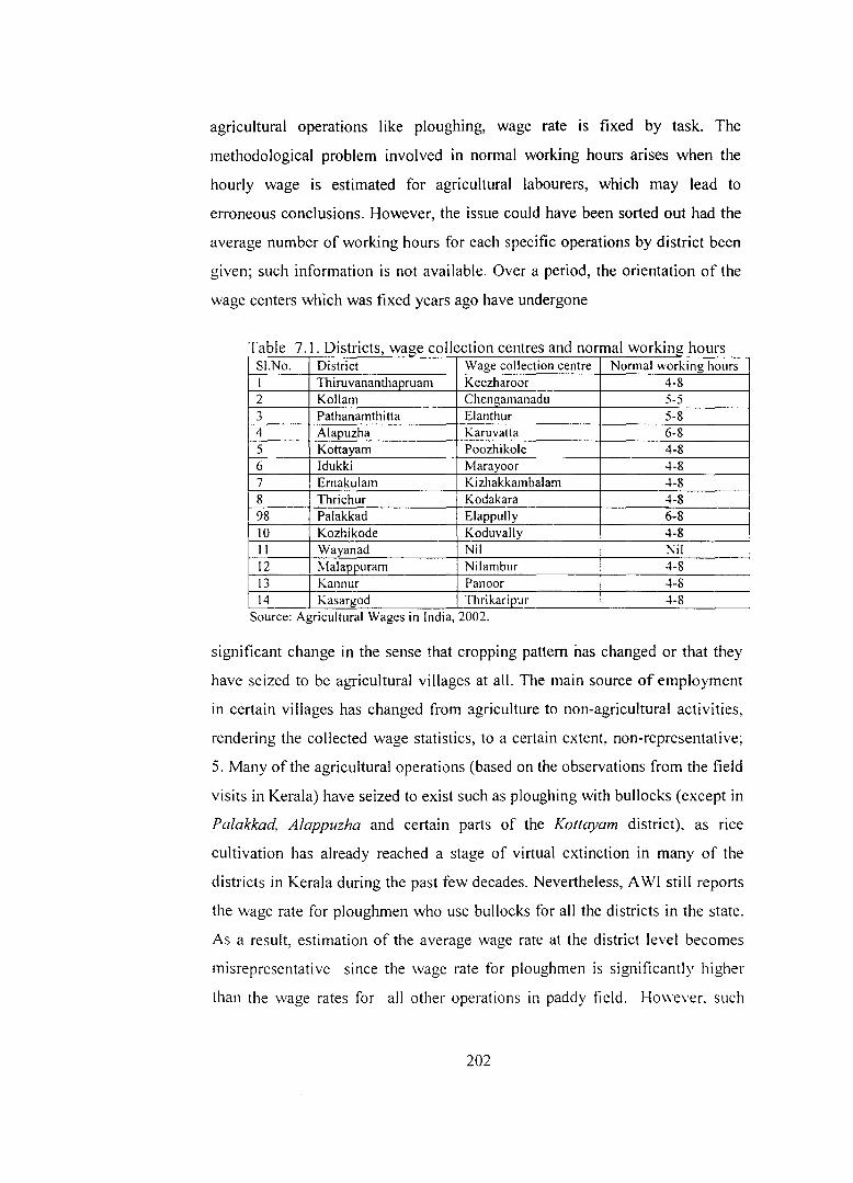
districts. Wayanad districe, which reports the lowest wage rate, is not at all

represented in the wage statistics. Information on Centres of wage collection in

Kerala and their respective districts along with normal working hours is

presented in Table 7.1. Normal working hours as reported in A WI ranged

between 4-8 hours. It is known that the normal working hours in every district

in the state for field (agricultural) labourers and that other agricultural

labourers ranged between seven and eight hours and only for certain specific

" Krishnaji, N. (1974). Wages of agricultural labourers. Economic and Political Weekly, VI (39): A-148- Al51. Jose, A.V.(1988). Agricultural wages in India. Economic and Political Weekzy, XXIII (26): A-46-A58; Srivastava, R. and Singh, R. (2005). Economic reform and agricultural wages in India. The Indian Journal of Labour Economics, 48(2):407-423; Himanushu, (2005). Wages in rural India: Sources, trends and comparability. The Indian Journal of Labour Economics. XXXXVIII (2): 375-406. 7 lt has already been mentioned elsewhere that the number of districts in Kerala has increased from I 0 in the 1960s to 14 in the 1980s by bifurcating the then existing districts as has happened in other states in India. It appears to be rather strange to note that the bifurcation of districts has not been communicated to the data-gathering agencies, which resulted in leaving the newly formed districts unlisted in the official list of data gathering agencies. As a result, wage data are not available or not collected from centers representing the newly bifurcated districts in Kerala. For example, Wayanad district is a hilly area wherein Tribals are the major sources of labour power to the agricultural sector. It is unfortunate to note that the district which registered the maximum casualty in the spate of farmers' suicides does not have representation in the list of centres of wage data collection either by the state governments or by the central governments. Even the Department of Economics and Statistics of the state government does not collect wage statistics from Wayanad district. Three districts which have historically been registering low wage rates in Kerala are Palakkad, ldukki and Wayanad. Among the three districts are historical data on the wage rate of rural labourers. vi::.., carpenter. mason and agricultural labour (Men) are available only for Palakkad district. Monthly wage statistics for different types of labourers in the rural labour households in ldukki district are avai !able in the Department of Economics and Statistics of Kerala on! y from 1998-99.

201

agricultural operations like ploughing, wage rate is fixed by task. The

methodological problem involved in normal working hours arises when the

hourly wage is estimated for agricultural labourers, which may lead to

erroneous conclusions. However, the issue could have been sorted out had the

average number of working hours for each specific operations by district been

given; such information is not available. Over a period, the orientation of the

wage centers which was fixed years ago have undergone

Table 7 1 Districts waae collection centres and normal workina hours '

.,.,. -SI.No. District Wage collection centre Normal working hours I Thiruvananthapruam Keezharoor 4-8 2 Kollam Chengamanadu 5-5 3 Pathanamthitta Elanthur 5-8 4 Alapuzha Karuvatta 6-8 5 Kottayam Poozhikole 4-8 6 Idukki Marayoor 4-8 7 Ernakulam Kizhakkambalam 4-8 8 Thrichur Kodakara 4-8 98 Palakkad Elappully 6-8 10 Kozhikode Koduvally 4-8 II Wayanad Nil Nil 12 Malappuram Nilambur 4-S 13 Kannur Panoor 4-8 14 Kasargod Thrikaripur 4-S

Source: Agncultural Wages m India, 2002.

significant change in the sense that cropping pattern nas changed or that they

have seized to be agricultural villages at all. The main source of employment

in certain villages has changed from agriculture to non-agricultural activities,

rendering the collected wage statistics, to a certain extent, non-representative;

5. Many ofthe agricultural operations (based on the observations from the field

visits in Kerala) have seized to exist such as ploughing with bullocks (except in

Palakkad, Alappuzha and certain parts of the Kottayam district), as rice

cultivation has already reached a stage of virtual extinction in many of the

districts in Kerala during the past few decades. Nevertheless, A WI still reports

the wage rate for ploughmen who use bullocks for all the districts in the state.

As a result, estimation of the average wage rate at the district level becomes

misrepresentative since the wage rate for ploughmen is significantly higher

than the wage rates for all other operations in paddy field. However. such

202

I I !

' '

problems could be resolved by assigning weights based on the workers

proportions. But such exercises are rather difficult to undertake since the

number of labourers or the hours or days of work are not reported along with

wage rates from the wage collection centers by concerned officials or the

government agencies.

The present study makes use of wage statistics supplied by RLE as well

as by Agriculture Wages in India. A WI wage data from RLE are used for inter­

state comparisons. As mentioned elsewhere, a major limitation of the wage

data furnished by NSSO-RLE is that the two data-gathering agencies

concerned at the national level do not supply information relating to the district

level. For the present study, time series data for different types of labourers in

rural areas at the district level, are inevitable. Even though Agricultural Wages

in India furnish wage rates for different types of labourers on a monthly basis

by agricultural operations, it is being observed that for many months

consecutively, wage data for certain types of labourers have not been given

furnished. For certain years, no entry could be found for a particular type of

labourers, compelling the researcher either to interpolate the data or leave them

as 'Not Available'. For the state, the wage data are supplied to the Ministry of

Agriculture by the Department of Economics and Statistics, Government of

Kerala. The State Department officials are deployed at the district level to

collect wage data from the centers, which have been identified long ago. It is

observed that the number of wage collection centres in every district have

declined over the years. On enquiry at the Ministry of Agriculture, it was

divulged that the delay in reporting wage rates from the respective states

compel the MoA to leave the column blank for certain agricultural operations

in the publication 'Agriculture Wages in India'.

The Department of Economics and Statistics, Government of Kerala,

collects wage statistics on important agricultural operations performed by male

and female labourers on behalf of the MoA and published in A WI. It may be

noted that wage rate for children have not been reported in A WI for many

years for Kerala, perhaps on account of the absence of the phenomenon in the

203

state. Even though wage details are collected for every agricultural operation,

the State Department consolidates the wages statistics only for the following

types of labourers, viz., carpenter and mason (rural), agricultural labour (men),

agricultural labour (women) and other agricultural labour (men and women).

For the first three categories, daily wage data on a monthly basis are available

in the State Department from 1958-59 onwards. The publication of wage

statistics series for agricultural Labour (women), Other Agricultural Labour

(men & women) was commenced only from 1973-74 onwards. An important

advantage of the wage data series collected and compiled by the State

Department is its availability for every month without break until 2005-06.

However, the Department of Economics and Statistics does not publish such

monthly wage data in any form and the annual averages for all these six types

of labourers are published in the Economic Review of the State Planning

Board. For the present study, district-wise monthly wage data consolidated for

the 4 7 year period for carpenter (rural), mason (rural) and agricultural labour

(men) and 27 year period data for agricultural labour (women), and other

agricultural labour (men and women) were copied down from the Wage

Registers maintained in the Office of the Department of Economics and

Statistics, Government of Kerala. It was reported that the data published by

the Department of Economic Affairs, MoA, are the restructured and

disaggregated versions prepared to suit the requirements of the conformity to

the general structure of the data published by A WI.

Wage data used in the study have the following limitations. i) Annual

averages and state averages are obtained by the unweighted simple average

method as there exist little information for assigning appropriate weights; ii)

The reported wage rate is consolidated form the Proforma filled in by officials

and there is little scope for seeking or receiving any explanation on wage

statistics because the proforma were filled at the district level and the office at

the headquarters in Thiruvananthapuram has only consolidated them. Even

though the wage data collected from the state department are the same as the

statistics published by MoA, the former have the following advantages; i)

204

Wage statistics are reported for e·1ery month from the collection centres and

for all the six categories of rural labourers. On the contrary, the wage statistics

published in A WI often leave columns vacant for many months for several

categories of labourers As a result, annual averages are calculated from the

information for two or three months; ii)A WI reports wage statistics only for 10

districts in Kerala, while the Department register reports wage rates for 13

districts. Precisely for these reasons, the present study is based on more

comprehensive and uninterrupted data series than that published elsewhere.

Section 2

7.2. Inter-state comparison of growth rates in wages

The vast literature on the trend and pattern of movement of wage rates

for agriculture labour reveal that the real wage rates had moved with

considerable fluctuations in its annual average growth rates for many of Indian

states since the mid 1960s. It was reported that the 1970s \\·itnessed a

deceleration in the rate of growth in the wage rate for agricultural labourers8.

Jose observed that the trend in the wage rate to decelerate was reversed in the

1980s in many states9. Notwithstanding the difference of opinion on the impact

of the neo-liberal economic policies on employment, wage-income and rural

poverty, researchers have arrived at a consensus that wage earnings of

agricultural labourers have not only seized to grow but also decelerated except

8 Krishnaji, N. (1971 ). Wages of agricultural labourers. Economic and political weekly, Vl(39): A 148-A 151. Jose, A.V.(1974). Trends in real wage rates of agricultural labourers. Economic and political weekly, IX(13): A25-A30. - (1988). Agricultural wages in India. Economic and politicalweekly,XXIII(26):A46-A58.; Sen, A.( 1994). Rural Labour markets and poverty. The Indian Journal of Labour Economics. XXXVII(4): 575-608. Parthasarthy, G. (1996). Recent trends in wages and employment of agricultural labour.lndian Journal of Agricultural Economics, 51 (I &2): 145-167. Shalla, S. ( 1997). Trends in poverty, wages and employment in India. The Indian Journal q( Labour Economics, 40(2): 213-223. Sarmah, S. (2002). Agricultural wages in India: A study of states and regions. The Indian Journal of Labour Economics, 44(1 ):89-116. 0

Jose. A.V.( 1988). Agricultural wages in India. Economic and political weekly. XXll/(26): A-46- A-58.

205

in the case of a few states in India during the 1990s10• On the contrary, it has

also been argued that the 1990s experienced acceleration in the real wage rate

of agricultural labourers 11•

Historically, daily wage earnings of agricultural labourers in Kerala

have been on a higher side as compared to other major states in India. Real

wage rates of male agricultural labourers in Kerala was Rs 3.8 against the

national average of Rs.1 . 70, the highest among 15 important states in India, in

1983. The real wage rate registered an average annual rate of growth of 5.7

percent per annum for the state (compound growth rate) while the national

average growth rate was 7.6 percent between the period 1983 and 1993-94 12•

In 1999-00, the real wage rate for agricultural labourers (male) in Kerala was

Rs 9.90 against the national average of Rs 4.30 and the rate of gro\\1h for the

state was 6 per cent per annum against the national average of 2.4 percent

between the period 1993 and 2000. These wage estimates were based on the

data series supplied by Rural Labour Enquiry Commission Report 13. On the

contrary, the rate of growth in the real wage rate for male agricultural labourers

in the state, based on the wage data from A WI, for the period 1981-91 and

1992-02 were 1.8 and 7.3 percent respectively 14• Kerala was reported to be

one ofthe few states in India, which had registered a higher growth rate in real

wage rate for agricultural labourers during 1990s as compared to 1980s.

Himanshu estimated the growth rates of real wages (at 1999-00 price) for

labourers engaged in agricultural operations from A WI as well as NSS-RLE

sources 15• It was found that the rate of growth in real wages for agricultural

10 Shalla, S. ( 1997). Trends in poverty, wages and employment in India. The Indian Journal of Labour Economics, 40(2}:213-223. Unni, J. ( 1997). Employment and wages among rural labours: Some recent trends. Indian Journal of Agricultural Economics, 52(1):59-72. 11 Sharma, H.R. (200 I). Employment and wage earnings of agricultural labourers: :\ state-wise analysis. Indian Journal of Labour Economics, 44(1 ): 27-38. 1

" Srivastava, R. and Singh, R.(2005). Economic reform and agricultural wages in India. The Indian Journal of Labour Economics, 48(2): 407-423. 13 Ibid 14

Ibid 15 Himanushu, (2005). Wages in rural India: Sources, trends and comparability. The Indian Journal of Labour Economics. 48(2): 3 75-406.

206

labourers was the highest during the period 1993-94 and 1999-00 (5.96%) as

compared to 1983-1987-88 (4.18%) and 1987-88 to 1993-94 (2.35%). On an

alternative estimate, employing wage data from NSS deflated with 1999-00

price index for agricultural labourers found that the rate of growth in the wage

rate for agricultural labourers (male) for the period 1993-94-1999-00 was 5.11,

which was again on a higher side when compared

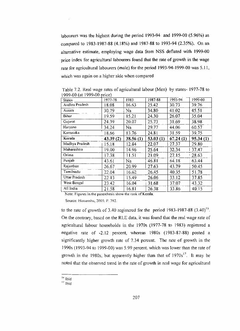
Table 7.2. Real wage rates of agricultural labour (Men) by states- 1977-78 to 1999-00 ( I 999 00 . ) at - pnce States 1977-78 1983 1987-88 Andhra Pradesh 18.08 16.63 25.42 Assam 30.79 Na 34.80 Bihar 19.59 15.21 24.30 Gujarat 24.39 20.07 25.73 Haryana 34.24 Na 29.77 Karnataka 18.66 13.76 24.81 Kcrala 43.39 (2) 38.56 (1) 53.03 (1) Madhya Pradesh 15.18 12.84 22.07 Maharashtra 19.00 14.96 25.64 Orissa 17.38 11.51 21.09 Punjab 43.61 Na 46.81 Rajasthan 26.67 20.99 27.63 Tamilnadu 22.04 16.62 26.45 Uttar Pradesh 22.13 15.49 26.06 West Bengal 23.42 16.04 31.68 All India 21.58 16.81 26.38 Note: F1gures 111 the parenthesis show the rank ofKerala.

Source: Himanshu, 2005: P. 392.

1993-94 1999-00

30.73 39.76 41.02 45.51 26.07 35.04 31.69 38.98 44.06 60.57 31.59 1 39.75 67.24 (1) 95.34 (1) 27.37 29.80 32.34 I 37.47 27.15 I 28.63 64.18 63.44 43.79 50.45 40.35 51.78 33.12 37.85 37.07 43.32 33.86 40.15

to the rate of growth of3.40 registered for the period 1983-1987-88 (3.40) 16.

On the contrary, based on the RLE data, it was found that the real wage rate of

agricultural labour households in the 1970s (1977-78 to 1983) registered a

negative rate of -2.12 percent, whereas 1980s (1983-87-88) posted a

significantly higher growth rate of 7.34 percent. The rate of growth in the

1990s (1993-94 to 1999-00) was 5.99 percent, which was lower than the rate of

growth in the 1980s, but apparently higher than that of 1970s 17• It may be

noted that the observed trend in the rate of growth in real wage for agricultural

16 Ibid 17 Ibid

207

labour households from the RLE source contradicts the rate of growth from

NSS and A WI. More or less the same trend could be observed for female

agricultural labour households as well. The long term trends in the real wage

rate of agricultural labour (men) in Kerala along with other states in India are

presented in Table 7.2. Important observations emerged from Table 7.2. are: i)

Real wage rate for labourers in Kerala had been growing at a rate faster than

Punjab, the second high wage state in India; ii) The difference in the wage

rates of agricultural labour (Men) between Kerala and Punjab has been

widening over the years particularly during the 1990s.

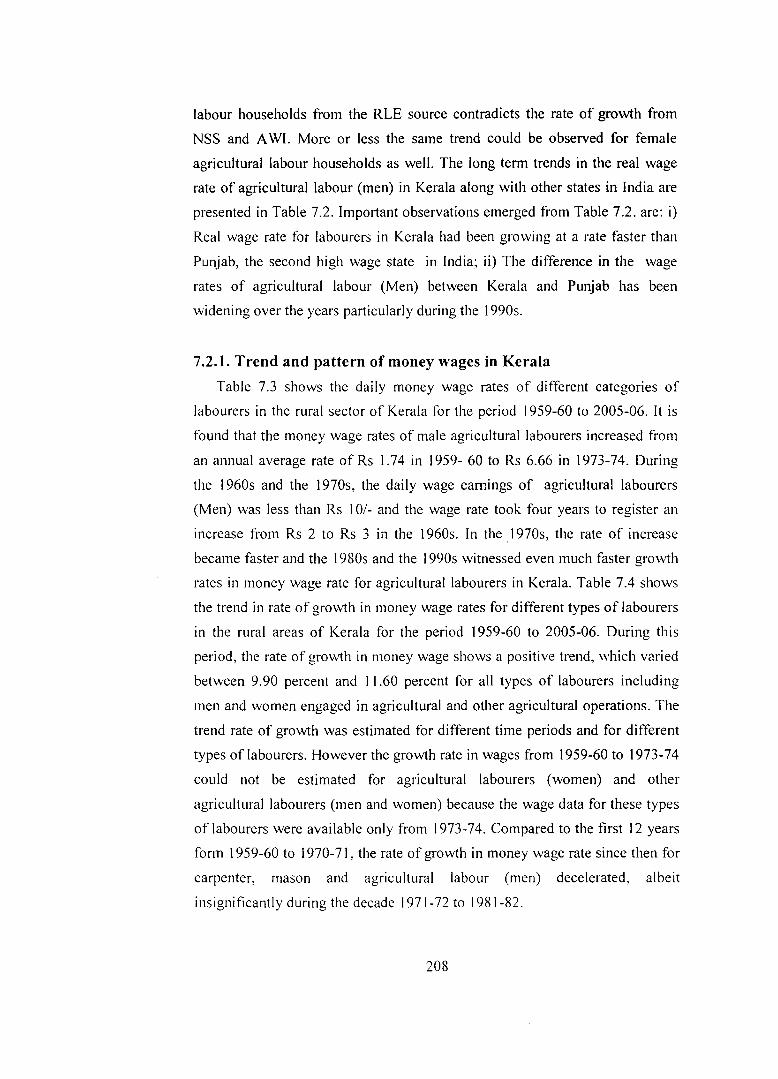
7.2.1. Trend and pattern of money wages in Kerala

Table 7.3 shows the daily money wage rates of different categories of

labourers in the rural sector of Kerala for the period 1959-60 to 2005-06. It is

found that the money wage rates of male agricultural labourers increased from

an annual average rate of Rs I. 74 in 1959- 60 to Rs 6.66 in 1973-74. During

the 1960s and the 1970s, the daily wage earnings of agricultural labourers

(Men) was less than Rs I 0/- and the wage rate took four years to register an

increase from Rs 2 to Rs 3 in the 1960s. In the _1970s, the rate of increase

became faster and the 1980s and the 1990s witnessed even much faster growth

rates in money wage rate for agricultural labourers in Kerala. Table 7.4 shows

the trend in rate of growth in money wage rates for different types of labourers

in the rural areas of Kerala for the period 1959-60 to 2005-06. During this

period, the rate of growth in money wage shows a positive trend, which varied

between 9.90 percent and 11.60 percent for all types of labourers including

men and women engaged in agricultural and other agricultural operations. The

trend rate of growth was estimated for different time periods and for different

types of labourers. However the growth rate in wages from 1959-60 to 1973-74

could not be estimated for agricultural labourers (women) and other

agricultural labourers (men and women) because the wage data for these types

of labourers were available only from 1973-74. Compared to the first 12 years

form 1959-60 to 1970-71, the rate of growth in money wage rate since then for

carpenter, mason and agricultural labour (men) decelerated, albeit

insignificantly during the decade 1971-72 to 1981-82.

208

Table 7.3. Money wage rates of rural labourers in Kerala-1959-60-2005-06 (Rs)

Year Carpenter Mason Agricultural Other Agricultural Coefficient Labour Labour of variation Men Women Men Women

1959-0 2.77 2.96 1.74 na na Na 0.264 1960-1 3.00 3.15 1.85 na na Na 0.266 1961-2 3.43 3.46 2.22 na na Na 0.233 1962-3 3.79 3.86 2.43 na na Na 0.240 1963-4 3.97 4.06 2.51 na na Na 0.248 1964-5 4.44 4.41 2.84 na na Na 0.235 1965-6 5.10 5.03 3.20 na na Na 0.243 1966-7 5.75 5.64 3.71 na na Na 0.228 1967-8 6.63 6.53 4.46 na na Na 0.209 1968-9 7.02 6.93 4.73 na na Na 0.208 1969-0 7.28 7.27 4.90 na na Na 0.211 1970-1 7.51 7.48 5.10 na na Na 0.207 1971-2 7.82 7.88 5.44 na na Na 0.197 1972-3 8.33 8.43 5.78 na na Na 0.200 1973-4 9.35 9.38 6.66 4.44 6.42 4.37 0.329 1974-5 11.13 11.19 8.03 5.37 7.75 5.31 0.321 1975-6 12.47 12.50 8.58 5.78 8.11 5.78 0.341 1976-7 13.46 13.62 8.44 5.89 8.25 6.02 0.374 1977-8 13.95 14.10 8.67 6.05 8.49 6.16 0.379 1978-9 14.41 14.39 8.97 6.26 8.31 6.33 0.382 1979-0 16.23 16.03 9.57 6.68 9.54 6.79 0.399 1980-1 19.81 19.85 11.13 7.91 11.10 8.27 0.419 1981-2 22.15 22.33 12.73 8.83 12.59 9.68 0.410 1982-3 23.43 23.51 13.53 9.55 13.39 10.43 0 401 1983-4 26.07 26.22 15.85 11.02 15.53 12.03 0.379 1984-5 38.73 38.72 23.59 14.12 23.27 16.58 0.412 1985-6 42.83 42.79 26.06 15.19 25.99 18.75 0.412 1986-7 45.93 45.93 28.39 16.38 29.16 20.66 0.401 1987-8 47.50 47.21 30.31 17.68 30.85 22.61 0.379 1988-9 49.80 49.55 31.95 18.66 32.41 23.59 0.378 1989-0 51.82 51.44 33.31 19.61 34.19 24.92 0.372 1990-1 54.47 53.99 35.73 21.07 36.79 26.35 0.363 1991-2 59.00 58.55 41.38 26.12 41.63 29.83 0.324 1992-3 67.67 67.65 48.38 32.30 49.20 35.99 0.300 1993-4 76.51 76.58 54.26 36.00 55.58 40.82 0.303 1994-5 87.41 86.95 63.53 42.22 65.09 49.71 0.283 1995-6 107.21 106.00 77.16 51.10 78.09 62.79 0.281 1996-7 128.54 127.85 92.18 60.52 91.80 76.96 0.283 1997-8 145.90 143.98 103.72 69.34 105.23 89.82 0.276 1998-9 155.43 155.01 111.23 71.39 108.60 93.16 0.291 1999-0 165.35 165.31 118.94 78.81 115.41 100.43 0.282 2000-1 177.04 174.23 125.24 86.12 124.10 103.42 0.281 2001-2 182.16 179.81 127.17 88.57 128.11 104.09 0.286 2002-3 190.43 186.71 137.52 92.95 142.95 106.61 0.280 2003-4 192.60 188.64 140.92 94.30 144.67 113.24 0.270 2004-5 199.34 195.02 144.33 96.19 148.37 123.83 0.266 2005-6 203.32 200.14 147.60 98.38 151.30 123.21 0.270 ,

Note : I. na denotes data not avaiiable2. For the agncultural labour (women) and for other agricultural labourers (men and women) data were available only from 1973-74.

Source: Department of Economics and Statistics, Government of Kerala.

209

During this ten year period, the rate of growth in money wage rates of

agricultural labour (men &women) was significantly lower than the rate of

growth for the entire period. It is worth mentioning in this context that the

reported deceleration in the rate of growth in money wage rate was found to be

less pronounced for the categories of carpenter, mason, and other agricultural

labourers (women). The daily wage rates of all types of rural labourers

experienced a hike in the rate of growth during the 1980s. The higher growth

rate in the daily earnings was found for agricultural labour (men) and other

agricultural labour (men & women) also. An important point emerging from

the Table 7.4 is that the deceleration in daily wage rates of rural labourers

happened during the 1990s and the early zeros were effect more or less

uniformly across the board. Broadly, rate of growth in money wages recorded

an accelerated growth rate in the 1980s, followed by a slow down during the

1990s and 2000s.

Table 7.4. Trend rate of growth in money wages of different type of labourers in the rural sector-Kerala

Period 1959-60 to 1959-60 1971-72

I 1981-82 1991-92

2005-06 to to to to Type of labourers 1970-71 1980-81 1990-91 2005-06 Carpenter

10.00 10.30 9.10 11.90 9.40

Mason 9.90 9.60 9.00 11.80 9.30

Agricultural labour 10.30 11.00 7.30 13.40 9.70

(Men) Agricultural labour

10.80 NA 11.00 10.80 9.40 (Women) Other Agricultural

11.10 NA 4.90 13.90 9.20 labour (men) I

Other Agricultural 11.60 NA 6.20 13.20 9.90

labour (Women) I. NA-not available 2 .. Daily wage rate for agricultural labour (women), other agricultural labour (men)

and other agricultural labour (women) were available only from 1973-74. Collection of wage statistics for these three categories in the rural sector was started only from the year in which it was available from the Department of Economics and Statistics, Government of Kerala as well as from the Agricultural Wages in India. Therefore, the trend rate of growth for these three categories for the phase starting from 1971-72 are related to 1973-74 to 1980-81 (7 years.) and for the overall growth rates, for these three type of labourers, it has been worked for the period 1973-74 to 2005-06. 3. Trend rate of growth is expressed in percentage and is obtained by trend gro\\1h rate. Source: Estimated from Table No.7.3

210

7.2.2. Trends in real wage rate in Kerala

Table 7.5 shows the real wage rate (at 1970-71 price) for different

categories of labourers in Kerala for the period 1959-60 to 2005-06. Money

wage rates for different categories of labourers were deflated with the

consumer price indices of agricultural labourers collected from the Department

of Economics and Statistics, Kerala 18 Real wage rate for agricultural labourers

(men) recorded a four fold increase while that of carpenter and mason

registered a three fold increase. The real wage rate for agricultural labourer

(men) was Rs 4.49 in 1973-74, which rose to Rs 11.35 in 2005-06. The real

wage rate for other agricultural labourers (men) registered an increase form Rs

4.32 in 1973-74 to Rs 11.64 in 2005-06 while that of women labourers

increased from Rs 2.94 toRs 9.48 during the same period. As observed in the

movement of money wages, different phases could be identified in the

movement of real wages as well.

Trend rates of growth in real wage for the different type of labourers are

presented in Table 7.6. For the entire period of analysis {1959-60 to 2005-06).

agricultural labourers (men) registered the highest rate of growth of 6.90

percent per annum followed by carpenters ( 4.29). For the same period, the real

wage rate of agricultural labour (women) and other agricultural labour (men &

women), grew at ranging from 3.23 percent and 3.96 percent.

During the 1990s and 2000s, wage rate has grown at a rate lower than

1980s except for carpenter and other agricultural labour (Men) (Table 7.6). The

observed pattern in the real wage rate is in sharp contradiction to the findings

on real wage rate of agricultural labourers based on the data series of A WI and

NSSO, but perfectly in conformity with the pattern obtained from the wage

series for rural labour households from RLE.

18 Data on consumer price index for agriculture labourers were collected from the Department

of Economics and Statistics. The consumer price index is related to the agricultural and other labourers. In the context of Kerala, this price index can be more meaningful for deflation. If adjustments were made for deflation/ reflation

211

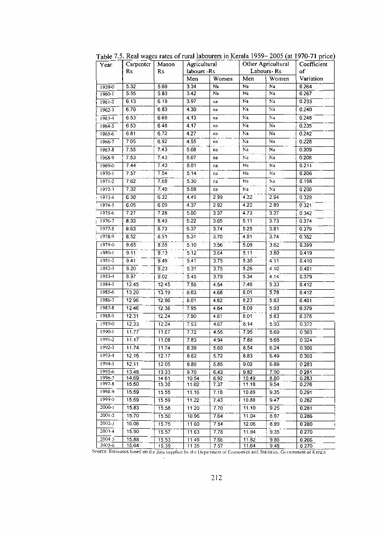
Table 7.5. Real wages rates ofrurallabourers in Kerala 1959-2005 (at 1970-71 price) Year Carpenter Mason Agricultural Other Agricultural Coefficient

Rs Rs labours -Rs Labours- Rs of Men Women Men Women Variation

1959-0 5.32 5.69 3.34 Na Na Na 0.264

1960-1 5.55 5.83 3.42 Na Na Na 0.267

1961-2 6.13 6.19 3.97 na Na Na 0.233

1962-3 6.70 6.83 4.30 na Na Na 0.240

1963-4 6.53 6.68 4.13 na Na Na 0.248

1964-5 6.53 6.48 4.17 na Na Na 0.235

1965-6 6.81 6.72 4.27 na Na Na 0.242

1966-7 7.05 6.92 4.55 na Na Na 0.228

1967-8 7.55 7.43 5.08 na Na Na 0.209

1968-9 7.53 7.43 5.07 na Na Na 0.208

1969-0 7.44 7.43 5.01 na Na Na 0.211

1970-1 7.57 7.54 5.14 na Na Na 0.206

1971-2 7.62 7.68 5.30 na Na Na 0.198

1972-3 7.32 7.40 5.08 na Na Na 0.200

1973-4 6.30 6.32 4.49 2.99 4.32 2.94 0.329

1974-5 6.05 6.09 4.37 2.92 4.22 2.89 0.321

1975-6 7.27 7.28 5.00 3.37 4.73 3.37 0.342

1976-7 8.33 8.43 5.22 3.65 5.11 3.73 0.374

1977-8 8.63 8.73 5.37 3.74 5.25 3.81 0.379

1978-9 8.52 8.51 5.31 3.70 4.91 3.74 0.382

1979-0 8.65 8.55 5.10 3.56 5.09 3.62 0.399

1980-1 9.11 9.13 5.12 3.64 5.11 3.80 0.419

1981-2 9.41 9.49 5.41 3.75 5.35 4.11 0.410

1982-3 9.20 9.23 5.31 3.75 5.26 4.10 0.401

1983-4 8.97 9.02 5.45 3.79 5.34 4.14 0.379

1984-5 12.45 12.45 7.58 4.54 7.48 5.33 0.412

1985-6 13.20 13.19 803 4.68 8.01 5.78 0.412

1986-7 12.96 12.96 8.01 4.62 8.23 5.83 0.401

1987-8 12.46 12.38 7.95 4.64 8.09 5.93 0.379

1988-9 12.31 12.24 7.90 4.61 8.01 5.83 0.378

1989-0 12.33 12.24 7.93 4.67 8.14 5.93 0.372

1990-1 11.77 11.67 7.72 4.55 7.95 5.69 0.363

1991-2 11.17 11.08 7.83 4.94 7.88 5.65 0.324

1992-3 11.74 11.74 8.39 5.60 8.54 6.24 0.300 1993-4 12.16 12.17 8.62 5.72 8.83 6.49 0.303

1994-5 12.11 12.05 8.80 5.85 9.02 6.89 0.283

1995-6 13.48 13.33 9.70 6.43 9.82 7.90 0.281 1996-7 14.69 14.61 10.54 6.92 10.49 8.80 0.283 1997-8 15.50 15.30 11.02 7.37 11.18 9.54 0.276 1998-9 15.59 15.55 11.16 7.16 10.89 9.35 0.291 1999-0 15.59 15.59 11.22 7.43 10.88 9.47 0.282 2000-1 15.83 15.58 11.20 7.70 11.10 9.25 0.281 2001-2 15.70 15.50 10.96 7.64 11.04 8.97 0.286 2002-3 16.06 15.75 11.60 7.84 12.06 8.99 0.280 2003-4 15.90 15.57 11.63 7.78 11.94 9.35 0.270 2004-5 15.88 15.53 11.49 7.66 11.82 9.86 0.266 2005-6 15.64 15.39 11.35 7.57 11.64 9.48 0.270

Source. Est1mates based on the data suppl1ed by the Depanment ot Economics and StatJStJcs, Gowmment ot Kerala

212

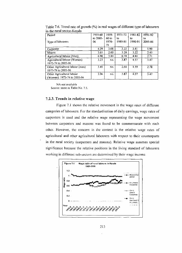
Table 7.6. Trend rate of growth(%) in real wages of different type of labourers in the rural sector-Kerala

Period 1959-60 1959- 1971-72 1981-82 1991-92 to 2005- 60 to to to to

Type of labourers 06 1970- 1980-81 1990-91 2005-06 71

Carpenter 4.29 3.08 3.22 3.41 5.90 Mason 3.61 2.00 3.20 3.22 2.45 Agricultural labour (Men) 6.90 3.80 0.70 4.80 2.71 Agricultural labour (Women) 3.23 NA 3.87 4.57 3.47 1973-74 to 2005-06 Other Agricultural labour (men) 3.45 NA 2.68 1.59 2.78 1973-74 to 2005-06 Other Agricultural labour 3.96 NA 3.87 4.57 3.47 (Women) 1973-74 to 2005-06

NA-not available Source: same as Table No. 7.5.

7.2.3. Trends in relative wage

Figure 7 .I shows the relative movement in the wage rates of different

categories of labourers. For the standardisation of daily earnings, wage rates of

carpenters is used and the relative wage representing the wage movement

between carpenters and masons was found to be commensurate with each

other. However, the concern in the context is the relative wage rates of

agricultural and other agricultural labourers with respect to their counterparts

in the rural society (carpenters and masons). Relative wage assumes special

significance because the relative positions in the living standard of labourers

working in different sub-sectors are determined by their wage income.

Figure 7.1 Wage ratio of rural labours in Kerala 1959-2006

1.2 -

0 penter 1 _ ................................................ . --+--- M ason/Ca

'! 0.8 ~ .... -~11"4~~~.-~~~ef'!I~~IJ<'e''l> ·--+--AL(men)/ ~ 0.6 _ Carpenter

0.4 .

0.2 -

213

-.-<,-··OA L (men)/ Carpenter

--CAL (women)/ 0 A L(men)

In the relative wage movement of agricultural labour (men) in relation

to carpenter (rural), three distinct phases are identified. The wage ratio of

agricultural labourers (men) with respect to carpenter increased from 0.63 to

0.72 during the period 1959-60 to 1974-75. The wage ratio started declining

by the mid 1970s and the phase of downturn continued upto 1990. It may be

noted that the observed deterioration in the relative wage rates of agricultural

labourers is attributable to the faster rates of growth of the daily \vage rates of

workers in the construction sector than a slow down in the growth rate of the

daily wages of agricultural labourers, as evidenced by the compound rate of

growth in money wages. The deterioration in the relative position of

agricultural labourers came to an end by the early 1990s and the wage ratio

between these two categories of labour started rising in favour of agricultural

labourers since the mid 1990s. The wage ratio between carpenters and

agricultural labourer (men) rose to 0. 73 in the 1990s and the observed trends in

the relative position in the daily earnings of other agricultural labourers with

respect to carpenters and masons (men and women) followed the suit.

7.2.4. Trends in product wage

Product wage is another variant of real wage. The former represents the

purchasing power of money wages measured in terms of the staple food (rice

in the present context) of the class of people in question while the latter

measures the purchasing power of a basket of commodities that can be

purchased with the money wage. Trends in the rate of growth in product wage

for different categories of labourers in rural Kerala are presented in Table 7.7.

It is seen that product wages also followed the same pattern as that of real

wages. The rates of growth in product wage was at an average rate of 3. 76

percent per annum for agricultural labour (men) during the period

214

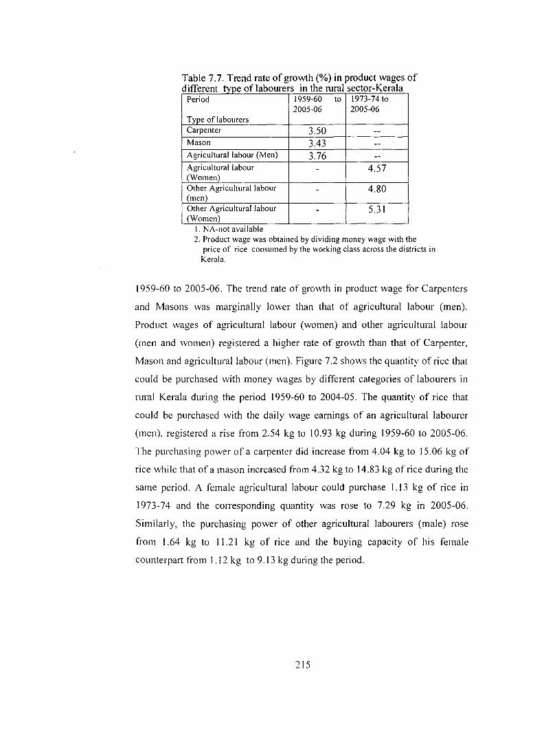
Table 7.7. Trend rate of growth(%) in product wages of d. ffl f I b . th I t K I I erent type o a ourers m erura sec or- era a

Period 1959-60 to 1973-74 to 2005-06 2005-06

Type of labourers Carpenter 3.50 --Mason 3.43 --Agricultural labour (Men) 3.76 --Agricultural labour - 4.57 (Women) Other Agricultural labour - 4.80 (men) Other Agricultural labour - 5.31 (Women)

I. NA-not available 2. Product wage was obtained by dividing money wage with the

price of rice consumed by the working class across the districts in Kerala.

1959-60 to 2005-06. The trend rate of growth in product wage for Carpenters

and Masons was marginally lower than that of agricultural labour (men).

Product wages of agricultural labour (women) and other agricultural labour

(men and women) registered a higher rate of growth than that of Carpenter,

Mason and agricultural labour (men). Figure 7.2 shows the quantity of rice that

could be purchased with money wages by different categories of labourers in

rural Kerala during the period 1959-60 to 2004-05. The quantity of rice that

could be purchased with the daily wage earnings of an agricultural labourer

(men), registered a rise from 2.54 kg to I 0.93 kg during 1959-60 to 2005-06.

The purchasing power of a carpenter did increase from 4.04 kg to 15.06 kg of

rice while that of a mason increased from 4.32 kg to 14.83 kg of rice during the

same period. A female agricultural labour could purchase 1.13 kg of rice in

1973-74 and the corresponding quantity was rose to 7.29 kg in 2005-06.

Similarly, the purchasing power of other agricultural labourers (male) rose

from 1.64 kg to I I .21 kg of rice and the buying capacity of his female

counterpart from 1.12 kg to 9.13 kg during the period.

215

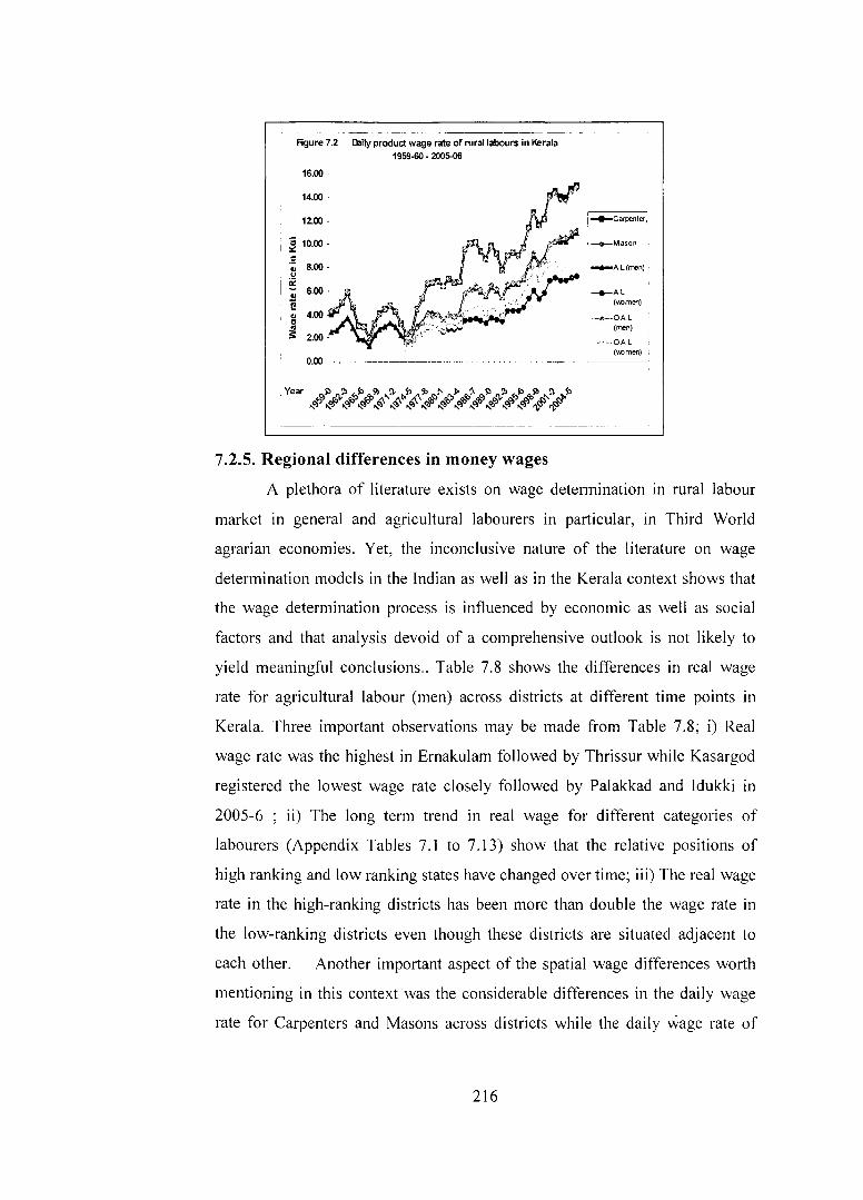
Figure 7.2 lllily product wage rate of rural labours in Kerala

16.00

14.00

12.00

I ~ 10.00-

·; 8.00 ~ .• !::! I~ ~

... 4.00

. " ~ 2.00"

1959-60 • 2005-06

0.00 --~·--·------------

·-+-Mason

--AL(men)

--Al (oomen) •

-+-0Al (men) I

.. QAL

------------- --~ ---------

7.2.5. Regional differences in money wages

A plethora of literature exists on wage determination in rural labour

market in general and agricultural labourers in particular, in Third World

agrarian economies. Yet, the inconclusive nature of the literature on wage

determination models in the Indian as well as in the Kerala context shows that

the wage determination process is influenced by economic as weii as social

factors and that analysis devoid of a comprehensive outlook is not likely to

yield meaningful conclusions .. Table 7.8 shows the differences in real wage

rate for agricultural labour (men) across districts at different time points in

Kerala. Three important observations may be made from Table 7.8; i) Real

wage rate was the highest in Ernakulam foiiowed by Thrissur while Kasargod

registered the lowest wage rate closely followed by Palakkad and Idukki in

2005-6 ; ii) The long term trend in real wage for different categories of

labourers (Appendix Tables 7.1 to 7.13) show that the relative positions of

high ranking and low ranking states have changed over time; iii) The real wage

rate in the high-ranking districts has been more than double the wage rate in

the low-ranking districts even though these districts are situated adjacent to

each other. Another important aspect of the spatial wage differences worth

mentioning in this context was the considerable differences in the daily wage

rate for Carpenters and Masons across districts while the daily wage rate of

216

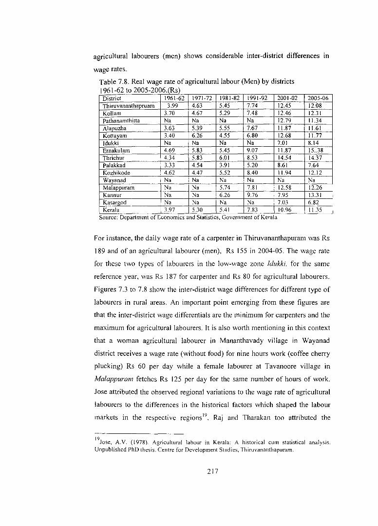
agricultural labourers (men) shows considerable inter'-district differences m

wage rates.

Table 7.8. Real wage rate of agricultural labour (Men) by districts 1961-62 to 2005-2006.(Rs) District 1961-62 1971-72 1981-82 1991-92 2001-02 2005-06 Thiruvananthapruam 3.99 4.63 5.45 7.74 12.45 12.08 Kollam 3.70 4.67 5.29 7.48 12.46 12.31 Pathanamthitta Na Na Na Na 12.79 11.34 A1apuzha 3.63 5.39 5.55 7.67 11.87 11.61 Kottayam 3.40 6.26 4.55 6.80 12.68 11.77 Idukki Na Na Na Na 7.01 8.14 Ernakulam 4.69 5.83 5.45 9.07 11.87 15 .. 38 Thrichur 4.34 5.83 6.01 8.53 14.54 14.37 Palakkad 3.33 4.54 3.91 5.20 8.61 7.64 Kozhikode 4.62 4.47 5.52 8.40 11.94 12.12 Wayan ad Na Na Na Na Na Na Malappuram Na Na 5.74 7.81 12.58 12.26 Kannur Na Na 6.26 9.76 7.95 13.31 Kasargod Na Na Na Na 7.03 6.82 Kerala 3.97 5.30 5.4 I 7.83 10.96 I 1.35

' Source: Department of Economics and Statistics, Government of Kerala

For instance, the daily wage rate of a carpenter in Thiruvananthapuram was Rs

189 and of an agricultural labourer (men), Rs 155 in 2004-05. The wage rate

for these two types of labourers in the low-wage zone ldukki. for the same

reference year, was Rs 187 for carpenter and Rs 80 for agricultural labourers.

Figures 7.3 to 7.8 show the inter-district wage differences for different type of

labourers in rural areas. An important point emerging from these figures are

that the inter-district wage differentials are the minimum for carpenters and the

maximum for agricultural labourers. It is also worth mentioning in this context

that a woman agricultural labourer in Mananthavady village in Wayanad

district receives a wage rate (without food) for nine hours work (coffee cherry

plucking) Rs 60 per day while a female labourer at Tavanoore village in

Malappuram fetches Rs 125 per day for the same number of hours of work.

Jose attributed the observed regional variations to the wage rate of agricultural

labourers to the differences in the historical factors which shaped the labour

markets in the respective regions 19• Raj and Tharakan too attributed the

19 Jose, A.V. (I 978). Agricultural labour in Kerala: A historical cum statistical analysis.

Unpublished PhD thesis. Centre for Development Studies, Thiruvananthapuram.

217

regional variation in wage rates across districts in Kerala to the differences in

the stage of development of agriculture20. They correlated real daily wage

earnings with Iand-man ratio across districts in Kerala21. In spite of a large

number of studies on different facets of wage determinations in the rural labour

market in Kerala, few studies discussed the spatial differences in the wage rate

for agricultural labourers within a region.

Regional differences in wage levels are explained in the political

economy frame work by ascribing them to the differences in the development

of the productive forces in agriculture and past struggles and unionisation of

labourers. On the contrary, in the supply-demand approach, inter and intra

spatial (district) differences in the wage rate for the same category of labourers

are sought to be explained by the regional differences in the supply of and

demand for labourers respectively. The land- man- ratio and the value added

per worker in the agricultural sector are the commonly employed two variables

to represent the supply of and demand for labourers. Empirical studies on inter­

district differences in agricultural wage are suggestive of the fact that the

supply-demand approach fails to explain inter-district wage differences as

districts are geographically positioned in such a way that they would promote

labour mobility22•

"0 Raj, K. N. and P.K.M.Tharakan, ( 1983). Agrarian reform in Kerala and its impact on the

rural economy: A preliminary assessment. In A.K. Ghose (ed.),Agrarian Reforms in Contempora~y Developing Countries. Crown Helm, London. PpJl-89. "

1 Ibid

"" Kerala is historically known for labour mobility. Commercial cultivation of plantation crops in the Malabar region was started mostly by migrant farmers from Travancore region. The migrant farmers were called 'Kudiyetta Karshalwr' It has recently been observed that labourers are migrating in large numbers from Thiruvananthapuram district, particularly from the Southern most part of the district (Neyattinlwra and Parasa/a) to various places in Central Travancore (Pa/a, Kanjirappally) in search of better employment opportunities particularly as tapping labourers in rubber plantations. As a result, wages for taping labourers in Kerala is more or less uniform across the state. The significant wage differential observed in the case of agricultural labourers in Kerala is therefore difficult to be explained simply in terms of supply and demand frame work indicating that the issue needs to be probed more in detail. (Field observations).

218

- ----~~---------

Figure 7.3

250

200

U) 150 ~ 1/)

~ 100

~ 50 "

0 --

Money wage of Carpenter 2004-05

Districts

---- - -------------------~-------

:Figure 7.4 Money wage rate of Mason 2004-05

250 -

200

150 U) ~

100 "' Q)

"' ~ 50

0

Figure 7.5

200 180 160 140 120

~ 100 -; 80 ~ 60 ~ 40

20

1 :~

~ ,.

~i :!IJ ~ 1i ~ I"'

liT '

Money wage of Agricultural labour (men) 2004-05

I ' -

0 - -=--='----""'- ,_ -- ~ -- - Ill

219

Districts

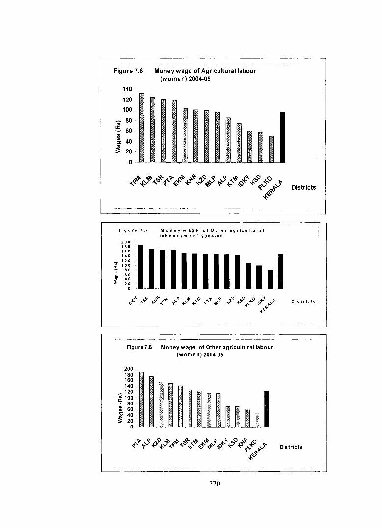
Figure 7.6 Money wage of Agricultural labour

140

120 4

100'

(ij' 80 .

a::: 60-1/J

~ 40 ~

;: 20 l '

(women) 2004-05

0 -!-''-

'\~~ *'-v~ '\c.,~~'\"?-~*'-~*'-~~~ ~.S ~ .¢'~ ~~ *'-C:J~v*'-~~ *"«;

Figure 7.7 Money wage ofOtheragricultural Ia b o u r ( m e n ) 2 0 0 4. 0 5

200 4

1 8 0 1 6 0 1 4 0

- 120 ~ 10 0 - 80 Ul Q) 60 Cl ~ 40 > 20

0 .lllllllllLtJ l -- - -- --- - --------~

Figure7.8 Money wage of Other agricultural labour

200 -180 4

160 140 . 120 ~

~ 100; --80 '

g: 60 I '"­

Cl 40 ! F ~ 2 I . > o -:I

0 - ~ -

(women) 2004-05

Districts'

Districts

Districts

------~--

220

It is observed that considerable differences exist in money wage real

wage rates for agricultural labourers across districts. The following

observations could be made from the trend in the wages rates across districts. i)

Differences in the wage rates for different type of labourers, as measured by

coefficients of variation, in districts such as Thiruvananthapuram. Kallam.

Pathanamthitta and Kozhikode narrowed down over the years and in the case

of other districts, difference in the wage rate widened over the years; ii)

Differences in wage rates for different type of labourers with in the district as

well as between districts are found to have widened in the 1980s across the

board and the observed trend can be attributed to the differences in wage hike

for labourers in the construction sector.

7.2.6. Phases of growth in money and real wages

Analysis of money and real wages of different types of labourers for

the period 1959-60 to 2005-06 clearly indicate that the long run movement in

the rate of growth of the different types of rural labour have not been uniform

as well as their counter part in the rural sector were not uniform during the past

four decades. Though the exact date of structural breaks in the long run

movement is not statistically tested, it is observed that the growth trend

registered a break in the early 1990s. To test the hypothesis, an instability

index in wage rates was estimated by dividing the period into two: the pre and

the post 1990s. Commonly employed statistical measure to estimate variability

is the coefficient of variation (CV). Variability measured using coefficient of

variation is not adjusted for the time trend. Given the downward sticky

characteristics of the wage rate (often labourers resist wage cuts ) instability in

the wage rate of any particular type of labourers is considered to share positive

trend as it would push the wage level upward to newer heights every time, it

gets destabilised. Instability in the daily real earnings of labourers is measured

employing Cuddy-Dulla Valle index23. The index take the following form:

"3

The Cuddy -Della Valle index takes into account the time trend in a variable, which is not captured in the coefficient ofvariation. The index is applied when a variable shows some

221

Instability Index= (CV*) ( 1-R1f 5

Where: CV* is the coefficient of variation ofthe series in percentage terms;

R2 is the explanatory power (adjusted for degrees of freedom) of OLS

regressed with time trend.

The null hypothesis put forward is that the real earning of rural labour

households as shown a higher degree of instability in the post-1990s as

compared to pre-1990s. The estimates obtained from the above exercise are

given in Table 7.9. The result clearly shows that the variability in the daily

wage rates of different types of labour was higher in the pre-1990 period than

in the period since 1990, which is indicative of the fact that the wage rates

experienced a higher positive rate of growth in the 1980s than in the 1990s.

The observed pattern is supportive of the trend in the rate of growth obtained

for the 1980s and the 1990s.

T bl 7 9 I a e bT . d nsta 1 It~ 111 ex o f rea wage rae SI.No Type of labourers Pre-1990 Post Total I

1990 I I Carpenter 11.58 3.84 13.61 2 Mason 10.84 4.04 13.53

-~ Agricultural labour (Men) 13.13 3.13 11.08 .)

4 Agricultural labour (Women) 3.73 2.72 8.49 5 Other agricultural labour (Men) 11.01 2.82 6.94 6 Other agricultural labour (Women) 8.122 4.79 8.05

Table 7.1 0. Estimated structural break dates in real wage rates for rural labourers Type of labourers 1st break 2"d Break 3'd break Carpenter (1959-60 to 2005-06)

1972-73 I 983-84 1994-95 Mason (I 959-60 to 2005-06)

1972-73 1983-84 1994-95 Agricultural labour (Men)

1971-72 1983-84 1994-95 ( 1959-60 to 2005-06) Agricultural labour (Women) 1980-81 Nil Nil ( 1973-74 to 2005-06) Other agricultural labour (Men)

I 983-84 1994-95 Nil Other Agricultural labour

1983-84 1994-95 Nil (women)

Note: Break pomts can also be obtamed w1th 95 percent confidence mterval.

trend which may be linear or non linear and in such cases Cuddy -Della Valle index is used as an appropriate measure of variability.

222

It has already been observed that the long run rate of growth in real and

money wage has not been uniform and has encountered a structural break.

The hypothesis can be statistically tested and the year of structural change

can be pin-pointed. The method commonly followed to estimate the

exponential trend in the growth of a variable can be expressed in the form

of the following equations .

y, = Yoe gt .................................. !

Logarithmic version in both sides ofthe equation gives

In Yt = In Yo+ g t + Ut ---------------------------------- 2

where Yt = is variable for which 'g' has to be estimated and Yo is the initial

year and Ut is the error term. The growth model assumes a constant rate of

growth for the entire period of the analysis. Apparently, such an assumption

deviates from reality because an economic variable like daily wage earnings,

which is subjected to frequent changes on account either of policy changes like

minimum wages or effected through other endogenous or exogenous variables.

The discussion on the long-run movement of real wages has categorically

pointed out that the real wage rates of different types of labourers in the rural

sector experienced a significant break in the 1970s and that a second break

took place in the 1990s. Often the long term trend in the rate of growth in

economic variables with such structural breaks is estimated by fitting a kinked

exponential function developed by Boyce24. It is assumed in such growth

models that the break took place exactly in the year in which the policy change

occurred. The kinked exponential function usually employed to work out the

rate of growth with an assumed year of break in the long run movement of the

wage takes the following form:

In y, = d, +a, (d,t + d2k) + ii2 (d2t- d2K) +u, ----- (3)

:• Boyce, J. K. ( 1986). Kinked exponential models for growth rate estimation. Oxford Bulletin of Economics and Statistics, 48(4):385-391.

223

where: In Y1 is the logarithmic version of real earning of labourers in the rural

sector; a 1 _ constant; a 1 • growth rate for the period 1 and d2 is the growth

rate for the period 2; K is the break point; dis dummy variable (1 and 0 as the

case may be) and U1 is the stochastic error term. This equation can be applied if

there is only one break or kink in the variable. If the number of kink extends to

four, the above equation takes the following form:

In Yr = ti1 + ii1 (d1t + d2k) + ii2 (d2t- d2K) + ii3 (d2t + d3k) + ii4 (d3t- d3K)+ iis(d3t + d4K) + ii6 (d4t- d4K) + 07 (d4l + dsK) + iia (dsl- dsK) + Ir--(3a;

As mentioned elsewhere, the estimation of long-term growth demands

a perfect knowledge of the variables and the variables in question. Often such

breaks are identified arbitrarily based on certain presumptions or with visual

judgment or graphical presentation of data. However, such identified break

points need not always be statistically valid or the result form the Chou test

would yield misleading result 25.

The presence or absence of a break in the long-run growth path of a

variable can be scientifically detected employing OLS-based CUSUM test

developed by Ploberger and Karmes (1996)26• OLS-based CUSUM test can be

used to make inference about the presence of a break in the variable in the

trend growth estimates based on equation-2. Structural break in the long run

trend can be detected statistically with the use of Cramer-Von Mises test

statistic procedure, which is used for the testing of the inference, and the test

statistic take the following form:u

" Hansen, B. E. (200 I). The new econometrics of structural change: Date breaks in US labour productivity. Journal of Economic Perspective, 15. 117-128. 26

The F test and the ordinary CUSUM are statistically not a valid proposition for a variable with the presence of trended repressors. The structural break in the long run movement of a

variable can be estimated statistically with the help of software called R. The software is available free of cost in the cite http:/www.R-project.org/ For a detailed elaboration of the application of structural break and CUSUM test, see K. Pushpangadan and Parameswaran (2006). Endogenous identification of growth phases: An Application to Kerala Economy . Working paper series, Centre for Development Studies, Thiruvananthapuram. Kerala (forthcoming).

224

Where u is the residual of the OLS regression of the full sample size T

and o is the standard error of the regression. The limiting distribution of the

test statistic F under the null hypothesis of no structural break can be defined

as tallows:

d st I FT ~X:> JB 2 (Z)dz

0

where d

S(

shows convergence m distribution, ~ is the stochastic

dominance and B2 (Z) is Brownian Bridge. The null hypothesis of no break

in the long term growth trend is rejected at a level of significance27 provided

the value of test statistic crosses the critical value28. It is important to note that

the procedure enables to detect the presence or absence of a break. However,

the year of the break and its corresponding growth rates are not supplied by the

test statistic. On having identified statistically the structural break in the long

run growth movement of the variable, kinked exponential growth rate

(Equation 3) can be used to estimate the rate of growth in each sub-period.

Table 7.10 shows the year of structural break in the long-run movement of real

wage for agricultural labour (men), agricultural labour (women), other

agricultural labour (men) and other agricultural labour (women). The break

years are statistically estimated using Bai and Pierre methodology and the

number of breaks are estimated based on minimum Bayesian Information

Criteria (BIC). The results presented in Table 7.10 show that there were three

major breaks in the long-run movement of the real wage rate for carpenter,

masons and other agricultural labour(men). It is worth noting in this context

that the statistically estimated breaks occurred for all the three categories of

labourers, a fact which indicates that the tum around in the regional economy

was not confined to any one particular sector or type of labour, but occurred

across the board. The first breaks in the real wage rate of carpenter and mason

occurred in 1972-73 and for agricultural labour (men), the break occurred in

the early 1970s. The second turnaround was simultaneous for all the· three

27 Ibid 28 Zeileis, eta/, (2005a). Monitoring structural change in dynamic econometric models. Journal of Applied Econometrics, 20: 99-121.

225

categories (1983-84) and the third break took place in 1993-94. For the other

three types of labourers, viz., agricultural labour (women), other agricultural

labourers (men and women), wage data were available only from 1973-74

onwards and therefore, the first phase in the long run movement of real wage

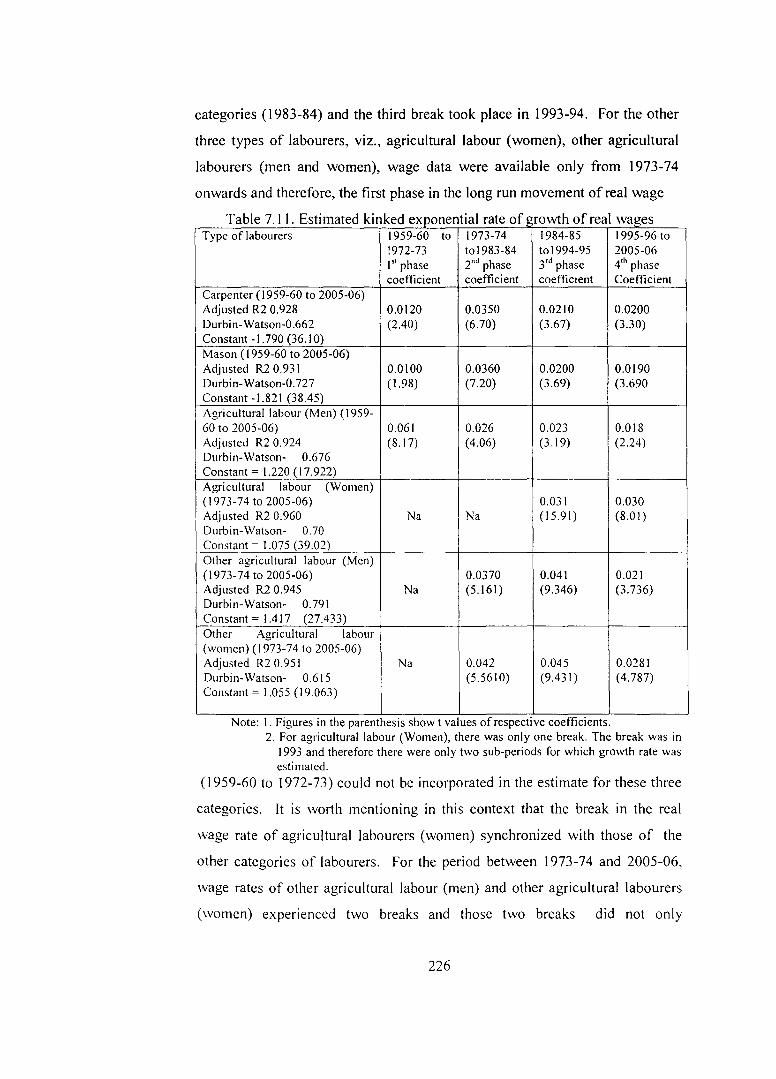
T bl 7 II E . a e sttmate d k. k d me . l f exponentta rate o ~ rowt h f 0 rea wages Type of labourers 1959-60 to 1973-74 1984-85 1995-96 to

!972-73 tol983-84 tol994-95 2005-06 I" phase 2"d phase 3'd phase 4'h phase coefficient coefficient coefficient Coefficient

Carpenter ( 1959-60 to 2005-06) Adjusted R2 0.928 0.0120 0.0350 0.0210 0.0200 Durbin-Watson-0.662 (2.40) (6.70) (3.67) (3.30) Constant -I. 790 (36.1 0) Mason ( 1959-60 to 2005-06) Adjusted R2 0.931 0.0100 0.0360 0.0200 0.0190 Durbin-Watson-0.727 (1.98) (7.20) (3.69) (3.690 Constant -1.821 (38.45) Agricultural labour (Men) (1959-60 to 2005-06) 0.061 0.026 0.023 0.018 Adjusted R2 0.924 (8.17) (4.06) (3.19) (2.24) Durbin-Watson- 0.676 Constant= 1.220 ( 17.922) Agricultural labour (Women) ( 1973-74 to 2005-06) 0.031 0.030 Adjusted R2 0.960 Na Na (15.91) (8.01) Durbin-Watson- 0.70 Constant= 1.075 (39.02) Other agricultural labour (Men) ( 1973-74 to 2005-06) 0.0370 0.041 0.021 Adjusted R2 0.945 Na (5.161) (9.346) (3.736) Durbin-Watson- 0.791 Constant = I .417 (27.433) Other Agricultural labour (women) (1973-74 to 2005-06) Adjusted R2 0.951 Na 0.042 0.045 0.0281 Durbin-Watson- 0.615 (5.5610) (9.431) (4.787) Constant = I .055 ( 19.063)

Note: I. F1gures 111 the parenthesis show t values of respective coefficients. 2. For agricultural labour (Women), there was only one break. The break was in

1993 and therefore there were only two sub-periods for which growth rate was estimated.

( 1959-60 to 1972-73) could not be incorporated in the estimate for these three

categories. It is worth mentioning in this context that the break in the real

wage rate of agricultural labourers (women) synchronized with those of the

other categories of labourers. For the period between 1973-74 and 2005-06,

wage rates of other agricultural labour (men) and other agricultural labourers

(women) experienced two breaks and those two breaks did not only

226

I

synchronise but did occur in the same year during which a serious turnaround

took place in the real wage rate of carpenters and masons.

On having identified the breaks points in the long-run movement of the

real wage data, a kinked exponential function was estimated. The advantage of

the kinked exponential model developed by Boyce29 is that it adjusts for the

kink by smoothing over the break points. Kinked exponential model imposes a

continuity restriction at the break point between sub periods to eliminate the

discontinuity bias, which would provide a better basis for comparison of the

growth in different sub-period30. When more than two sub-periods are

incorporated in the kinked exponential function, the equation specified above

would take the form for four sub-periods. The rates of growth for the different

sub-periods identified through the breaks are presented in Table 7 .II. It may

be noted that four growth rates corresponding to three breaks including the one

for the last period can be obtained. The following observations may be made

from the estimated growth rates for the sub-periods. i) The real wage rate of

carpenters and masons registered relatively low growth rates in the first phase

( 1959-60 to 1972-73). In the second phase, these two categories of labourers

recorded the highest growth rate (1973-74 to 1982-83), ii) Rates of growth in

the real wage rate for all the six types of labourers considered in this section

recorded were the lowest in the last phase ( 1993-94 to 2005-06), a finding

which matches well with the earlier findings in the growth rates observed

earlier; iii) Real wage rate recorded the highest growth rate for agricultural

labourer (men) in the first phase and the lowest for the category in the last

phase (1993-94 to 2005-06); iv) Wage rate for other agricultural labour (men)

recorded a reasonably higher growth rate in the second phase and a poor

growth rate in the last phase. The same trend is observed for other agricultural

labourers (women) as well. There were only two phases in the long-run wage

movement of women labourers and further the first phase (1973-74 to 1993-

~Q Boyce, J. K. (1986). Kinked exponential models for growth rate estimation. Oxford Bulletin of Economics and Statistics, 48(4):385-391. 30

Pushpangadan, K.(l990).Methods in applied economics. Centre for Development Studies, Trivanadrum, Kerala. Pp.l-43.

227

94) registered a growth rate, which was not significantly different from that in

the last phases. The phases identified in the long run real wage movement for

all the six types of labourers in the rural sector categorically show that the

period from 1993 experienced a significant slow down in contrast with the

earlier findings of the wage rate movement in Kerala. Moreover, the rates of

growth by phases match very well with the phase- wise growth rate estimated

with discontinued series and the overall growth pattern of the state domestic

product of the regional economy. In brief, it may be stated that the wage rates

of rural labour households in Kerala registered a higher growth in the 1980s

and a lower growth rate in the 1990s, which is in contradiction to the findings

of studies based on the data from A WI and NSSO but in conformity with the

real wage rate of agricultural labour household reported by RLE. It is a clear

indication of the fact that the two distinct phases could be identified in the

long- run wage movement of rural labour households as pre 1991 and post-

1991.

Section 3

7.3. Rural wage determination

In this section, an attempt is made to identify important factors, which

influence daily wage rates of agricultural labourers across the districts of

Kerala. As discussed in chapter 2, literature on the labour market IS

overwhelmingly dominated by econometric models of wage determination.

These models are confined mostly to the supply- demand framework. Supply

of and demand for labourers assume importance even in the political economy

framework too. Variations in wage rates in the short-run are determined by the

supply-demand factors. The underlying economic logic of the supply-demand

framework is that labourers (factors of production) move from low wage

(price) zones to high wage zones followed by equalisation of wages or prices.

Though the labour market in the Kerala context has been sufficiently

analysed, the literature based on econometric modeling is very few and far

228

between and the relationship between wages and the other related economic

variables are yet to be studied in great detail. Existing studies on rural wage

determination were focused on gauging the impact of wage hike on the

material production sector of the economy. Even though the very objective of

the econometric modeling by Krishnan too falls in this category, his exercise

be considered the first serious exploration into the wage structure in the

informal sector with special emphasis on agricultural labourers in Kerala31•

Krishnan sought to explain the wage differentials by inter-relationships of

rural labour markets32. Wages are inter-related because a hierarchical order

exists in the wage structure and therefore in the long run, relativity in the

hierarchical order would be maintained to stabilise wage parity. Krishnan

argued that changes in wage level, especially in the upward direction, included

two components, viz., initial change(causal factors) and induced change

(structural factors). In the hierarchical order of the wage structure, any change

effected in the upper rung of the wage hierarchy gets transmitted to the bottom

through the structural factors. It was observed that the boom in the construction

sector driven by the remittance flow from West Asian countries, resulted in a

hike (causal factor or initial change) in wage rates of carpenters and masons,

which induced a change in the wage rates of agricultural labourers during the

1970s. To test for the causal as well as feed back effects, Vector Auto

Regressive model (VAR) was estimated and tested or Granger causality-Sims's

test. 33 Krishnan could observe four types of causalities as described below34.

31 Krishnan, T.N. (1991 ). Wages, employment and output in interrelated labour market in an agrarian economy: A study of Kerala. Economic and political weekly, XXVI(26):. A-82- A-96. 32 Ibid. 33 In the case of simultaneous or structural equations, certain variables are assumed to be endogenous and others exogenous. In such equations, even before estimation, equations are identified and often it is assumed that some of the predictor variables are present only in some equations. This assumption makes the model rigid alternative proposition was suggested by Christopher Sims. According to Sims, if there is simultaneity among a set of variables, they should all be treaded on equal footings and further apriori distinction between endogenous and exogenous variables in the equation need to be removed. Granger Causality-Sims's test treats all variables as endogenous and if the predictor variables are multiple in number, Vector Auto Regression (V AR) model is used. The term V AR refers to lagged value of the dependent variable on right-hand side of the specification and vector refers to the vector of variables. The basic premise of V AR is that future values of X depend on the current and the past values of X

229

I. Between rural and urban wages

2. Between skilled and unskilled labourers

3. Between masons' helpers and agricultural labourers

4. Between men agricultural labourers and women agricultural labourers.

Granger-Sims's causality test clearly showed that the wage hike in the

sector was transmitted on to the rural labour market in Kerala. It could also be

found that a hike in wage induced changes in prices of wage goods as well. If

the argument is accepted, the question which remains unanswered is the factor

which triggered the 'initial change'. Secondly, Krishnan postulated that

changes in the product market destabilise the wage relativity in the short-run

but only to restore it in the long run. If the product demand stagnates for a

fairly long period, wages for the particular segment in the labour market would

not move in tandem with the hierarchical order as envisaged in the wage

relatively hypothesis or wage structure. It is not clear which way the wage

parity is achieved if the product market remains slack in the long-run. Wage

relativity as a theoretical concept is therefore inadequate to explain the spatial

differences in wage rates. The inter-related labour market theory postulates that

collective bargaining or trade unions have little role to play in determining the

only and the presence or absence of causality is detennined by the significance of 'F' test. F

( Rss R - RSS ur ) I m test is given by the formula: F= --------'---

RSS ur I m ( n - k ) Where RSS R stands for the residual sum of squares of the lagged values of the X variables and in the regression, the other variables (if wage hike causes price change) only the lagged values of wages and other X variables are used and not of prices. RSSur stands for the residual values of the sum of squares of the equation in which price is theY variable and lagged values of the price is the X variable along with other variables except wage. It follows F distribution with m

and (n-k) df. The null hypothesis H0 = L a = 0. If the computed F value crosses the

critical F value at the chosen level of significance, the null hypothesis is rejected indicating that there is causal relationship between wage and the price of commodities. The V AR model specified in the inter related labour market took the following form.

Wag," f,,Msn ,_ 1• f,;Wagl ,_ 1 '11, I=! 1=1

where Wag, is the wage rate of agricultural labour (men) in the current year and \Vag,_ 1 is the wage rate of same in the last year (12 months lag) and Wmsn ,_ 1 is the wage rate of masons' helper in the last year. " Krishnan, T.N. (1991 ). Wages, employment and output in interrelated labour market in an agrarian economy: A study of Kerala. Economic and political Weekly, XXVI(26): A-82- A-96.

230

wage levels, an association which is very much against the history of wage

movement and labour struggle in Kerala. In the above context, it is difficult to

accept the inter-related labour market theory as a satisfactory model to explain

the wage movements or inter-district wage variation.

In a supply-demand frame work, variables often used to represent the

demand for labourers are: i). Labour productivity measured in terms of the

value added per worker or area of land cultivated; ii) General economic

performance measured in terms of the rate of growth in Net State Domestic

Product (NSDP); iii) Percentage of area under food and non-food crops; iv)

Proportion of area irrigated to total cropped area; v) Capital investment per

unit of land or labour; vii) Government expenditure on self-employment and

poverty alleviation programmes. Important supply side variables are: i)

Proportion of agricultural labourers in the total workers; ii) Number of

agricultural labourers per hectare of land; and iii) Proportion of non-farm

workers to total workers. Srivastava and Singh constructed an elaborate

econometric model with alternative specifications of the variables on the

demand and the supply sides with time-series as well as panel data for 14

important states in India 35. The study observed that the rate of growth in real

wages for agricultural workers is influenced by the demand factors such as the

performance of the agricultural sector reflected in the rate of growth in net

value added per agricultural labourer, area expansion under non-food grains,

area under irrigation and agricultural productivity. The important supply side

factor was the degree of diversification of rural workforce36.

7.3.1 District-wise model for wage determination

In a district-wise analysis of daily wages characterised by significant

differences across districts, it is important to know whether the slope (p) and

intercept (a) are significantly different across districts. A multi-step Chow test

procedure is sufficient to reveal whether the regressions for different districts

-" Srivastava, R. and Richa Sing. (2005). Economic reforms and agricultural wages in India. The Indian Journal of Labour Economics, 48(2):407-423. 36 Ibid.

231

over time are comparable. It is also useful in the present context to examine the

source of the differences in the regression estimates, which could be on

account of the differences in the slopes or the intercepts. In this case the model

can be specified as equation 1.

-------- 1

where Y1 is the dependent variable and D21 is the time dummy. Xr is the array of

independent variable and D2X;1 is the slope of the interactive dummy.

In the light of the observed significant variations in the daily wage rate

across districts in Kerala, it is impot1ant to identify the variables on the supply

side and on the demand side, for each district. At the district level, availability

of comparable data poses a serious problem. Limitations in data at the district

level are given below:

1. Time series data on wage rate are not available for all districts for the period

from 1958-59 to 2005-06. For the Wayanad district, wage data are not

collected at all. f"or certain other districts, wage data are available only

from 1988-89. Historical wage data for Manathavady Panchayat was

available from the Development Report of the Grama Panchayat and also

from village records;

2. An important variable on the demand side is value added from agriculture

in NSDP at the district level at constant price. At the district level, value

added from agriculture is available only from 1995-96;

3. District-wise details on capital investment, development expenditure and

government spending on poverty alleviation programmes and alternative

employment generating schemes are hard to come by. Regression variables

and sources of data are presented in Table 7.12. The panel data include the

time series data from 1995-96 to 2003-04 for 14 districts. The advantages

of the panel data over cross section or time series data are well known37.

37 Gujarati. D.N. (1995). Basic econometrics. McGraw-Hill Book Co., Singapore, pp. 499-

539.

232

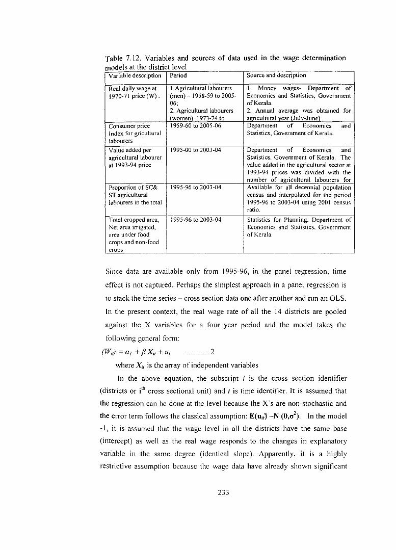
Table 7.12. Variables and sources of data used in the wage determination models at the district level

Variable description Period Source and description

Real daily wage at !.Agricultural labourers I. Money wages- Department of 1970-71 price (W) . (men)- 1958-59 to 2005- Economics and Statistics, Government

06; ofKerala. 2. Agricultural labourers 2. Annual average was obtained for (women) 1973-74 to agricultural year {July-June)

Consumer price 1959-60 to 2005-06 Department of Economics and Index for gricultural Statistics, Government of Kerala. labourers

Value added per 1995-00 to 2003-04 Department of Economics and agricultural labourer Statistics, Government of Kerala. The at 1993-94 price value added in the agricultural sector at

1993-94 prices was divided with the number of agricultural labourers for

Proportion of SC& 1995-96 to 2003-04 Available for all decennial population ST agricultural census and interpolated for the period labourers in the total 1995-96 to 2003-04 using 200 I census

ratio.

Total cropped area, 1995-96 to 2003-04 Statistics for Planning. Department of Net area irrigated, Economics and Statistics. Government area under food ofKerala. crops and non-food crops

Since data are availabie only from 1995-96, in the panel regression, time

effect is not captured. Perhaps the simplest approach in a panel regression is

to stack the time series- cross section data one after another and run an OLS.

In the present context, the real wage rate of all the 14 districts are pooled

against the X variables for a four year period and the model takes the

following general form:

(W;J = o.1 + f3 xit + u1 ------------ 2

where Xit is the array of independent variables

In the above equation, the subscript i is the cross section identifier

(districts or ith cross sectional unit) and t is time identifier. It is assumed that

the regression can be done at the level because the X's are non-stochastic and

the error term follows the classical assumption: E(ui.J -N (O,a2). In the model

-I, it is assumed that the wage level in all the districts have the same base

(intercept) as well as the real wage responds to the changes in explanatory

variable in the same degree (identical slope). Apparently, it is a highly

restrictive assumption because the wage data have already shovm significant

2.,., -'-'

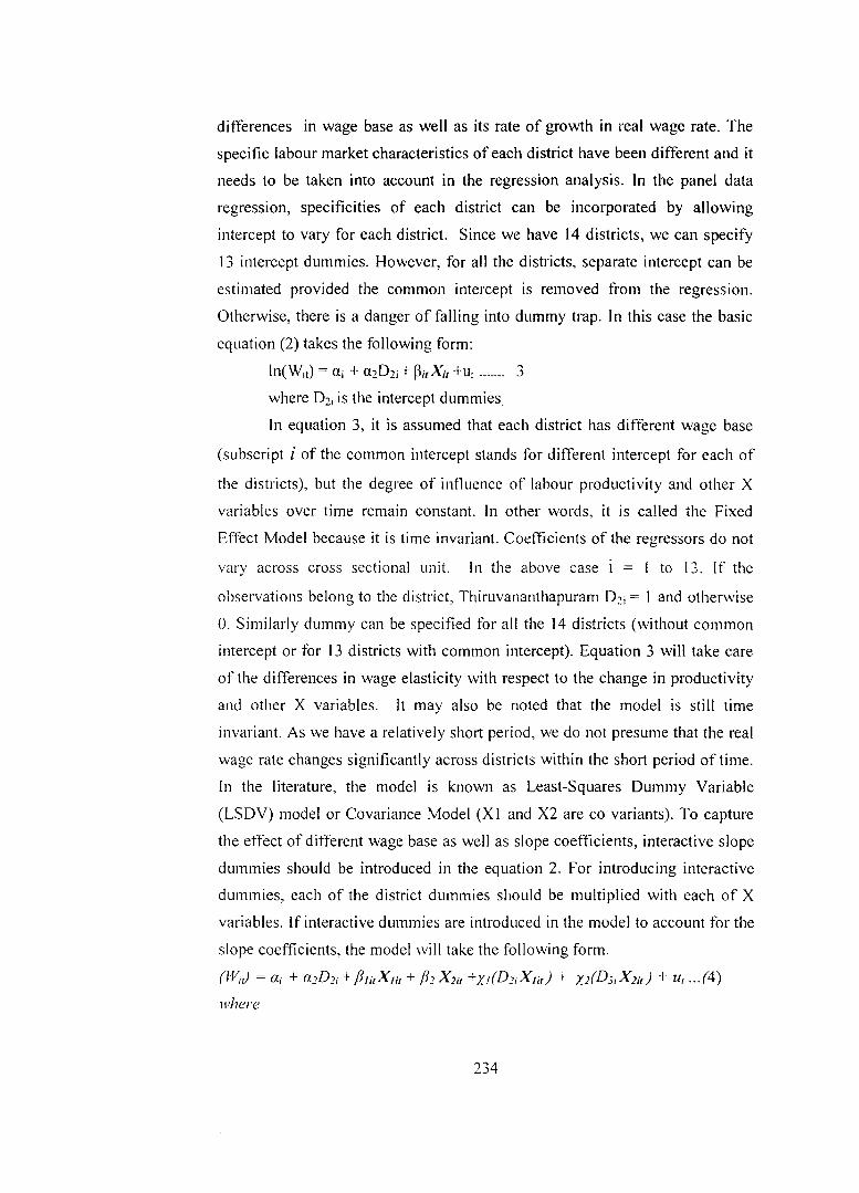
differences in wage base as well as its rate of growth in real wage rate. The

specific labour market characteristics of each district have been different and it

needs to be taken into account in the regression analysis. In the panel data

regression, specificities of each district can be incorporated by allowing

intercept to vary for each district. Since we have 14 districts, we can specify

13 intercept dummies. However, for all the districts, separate intercept can be

estimated provided the common intercept is removed from the regression.

Otherwise, there is a danger of falling into dummy trap. In this case the basic

equation (2) takes the following form:

ln(W;t) =a; + azD2; + ~;tXit +ut ·------ 3

where 0 2; is the intercept dummies

In equation 3, it is assumed that each district has different wage base

(subscript i of the common intercept stands for different intercept for each of

the districts), but the degree of influence of labour productivity and other X

variables over time remain constant. In other words, it is called the Fixed

Effect Model because it is time invariant. Coefficients of the regressors do not

vary across cross sectional unit. In the above case i = I to 13. If the

observations belong to the district, Thiruvananthapuram 0 2; = 1 and otherwise

0. Similarly dummy can be specified for all the 14 districts (without common

intercept or for 13 districts with common intercept). Equation 3 will take care

of the differences in wage elasticity with respect to the change in productivity

and other X variables. It may also be noted that the model is still time

invariant. As we have a relatively short period, we do not presume that the real

wage rate changes significantly across districts within the short period of time.

In the literature, the model is known as Least-Squares Dummy Variable

(LSDV) model or Covariance Model (XI and X2 are co variants). To capture

the effect of different wage base as well as slope coefficients, interactive slope

dummies should be introduced in the equation 2. For introducing interactive

dummies, each of the district dummies should be multiplied with each of X

variables. If interactive dummies are introduced in the model to account for the

slope coefficients, the model will take the following form.

(W;J = 0.; + a.2D2i + f31itxlit + /32 x2it +xJ(DJ;X/it) + XJ(Ds;Xlit) + Ur ... (4)

where

234

(D2i X 1 it) is the dummy interactive term for the X1 and so on. In the present

context, the degrees of freedom do not permit the introduction of additional

variables into the model. Therefore, we are rather forced to limit to the

differential intercept dummies. In the case of intercept dummies, the two

models with and without intercept dummies can be compared with the

restricted F test. The intercept dummies level of significance can be tested by

comparing the P values of the estimated t coefficients. The intercept values of

each district can be obtained by adding to the individual intercepts, the

intercept value of the control district or the common intercept. If the district­

wise intercepts are statistically different from one another, the wage bases of

districts are not comparable at all. The result obtained from the Fixed effect

model showed that the dummies were significant which indicated that the wage

base of the districts were different. However, the low explanatory pO\ver ofthe

equation (R2) unsatisfactory OW and P values were indicative of the weak

relationship and multicolleniarity problem and it could not be corrected as the

degrees of freedom did substantially reduce with the introduction of many

dummy variables in the equation. The result was not found worth reporting.

The availability of data for a relatively shorter period did perhaps not permit

the introduction of many dummy variables into an equation.

To begin with, Pearson correlation coefficient was computed to explore

the inter-relationship between real wage rate and other variables in the demand

and supply sides. Correlation coefficients are reported in Table 7.13. It was

found that real wage rate of agricultural labour (men) was positive and

significant with the demand side variables, viz., value added per hectare of

cropped area, area under non-food crops and net district domestic product.

Real wage rate was found to be negative and significant with the area under

food crops. Supply side variables included in the correlation analysis were: i)

Percentage of agricultural labourers in the total main workforce; ii) Number of

agricultural labourers per hectare of total cropped area; iii) Percentage of SC

and ST in the total population. Except the number of agricultural labourers per

hectare of land, other two variables bore expected negative sign with

significance at I% level.

235

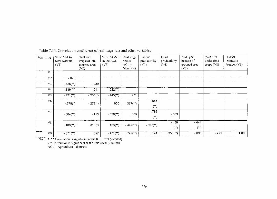
Table 7.13. Correlation coefficient of real wage rate and other variables

Variable %of AGLto %of area %of SC/ST total workers irrigated total in the AGL (VI) cropped area (V3)

(V2) VI

V2 -.073

V3 .726(**) -.089

V4 -.589(**) .011 -.522(**)

vs -.721 (**) -.265(*) -.445(**)

V6 -.279(*) -.278(*) .000

V7 -.664(**) -.113 -.538(**)

vs .486(**) .318(*) .426(**)

V9 -.571 (**) .057 -.471(**)

Note : I. ** Correlation IS significant at the 0.0 I level (2-taiied) 2. * Correlation is significant at the 0.05 level (2-tailed). AGL- Agricultural labourers

Real wage Labour rate of productivity AGL- (V5) Men (V4)

.231

.565 .367(**)

(**)

.788 .006

(**)

-.447(**) -.667(**)

.749(**) .141

Land AGL per %of area District productivity hectare of under food Domestic (V6) cropped area crops (V8) Product (V9)

(V7)

-.063

-.488 -.444

(**) (**)

.353(**) -.093 -.221 1.00.

Regression model-1;

Based on the result of correlation coefficient, regression coefficients

were estimated (adequate changes were made in the variables for regression)

with alternative specifications and the variables were finalised through trial

and error method. Results of regressions with alternative specifications and

satisfactory R2, DW and 't' are presented in Tables 7.14, 7.15, 7.16 and

7.17.

In model I, area irrigated, Net District Domestic Product at constant

pnce, area under food crops (demand side variables) and total number

agricultural labourers (supply side variable) were regressed against the real

wage rate for agricultural labourers. The result of the model is reported in

Table 7.14. It was found that the model could explain 73 percent of the

variations in real wage rate (Adjusted R2). It was also found that one unit

change in the overall income of the district (general development) brings in

0.42 unit change in real wage rate. Area irrigated was found to be an

insignificant factor in stimulating the demand for labourers and thereby the

vvage rate because the cultivation in the state is mostly rain-dependent except

in Palakkad district. It is also interesting to note that the area under food crops

showed a negative and significant relationship with the real wage rate. This

result may be viewed in the backdrop of the sharp decline in area under paddy

and tapioca cultivation except in Palakkad and Alapuzha districts. Palakkad is

one of the low-wage zone and Alapuzha is a medium wage zone in Kerala.

However, the observed relationship that one unit decline in area under food

crops brings in 0.30 unit increase in wage rate calls for further explanation.

Natural rubber cultivation replaced tapioca in almost every part ofthe dryland

in Kerala. The fall in the days of employment on account of the decline in

paddy and tapioca cultivation forced a section of the agricultural labourers

(young and able bodied) to migrate to booming sectors and those who did not

migrate were aged males and female labourers from Scheduled castes, who had

already withdrawn from the labour market. It virtually left very few

237

agricultural labourers in the sector and the existing labourers demanded a wage

rate on par with the rate existing in the construction sector where they or their

fellow labourers work. Moreover, for a very few jobs in the agricultural sector,

the existing labourers too demanded a higher wage rate because the available

number of days of employment was less than ten days in a month even for an

able bodied labourer. It is, therefore, logical that the decline in employment

days forces out labourers from the sector faster than the decline in the days of

employment and a few jobs left in the sunset sector has to attract labourers

from the allied sectors for which the wage rate has to be paid on par with other

sectors. The strong and significant association between wage rate and district

domestic product reflects that the existing wage rate has little relation with the

development of agriculture but the overall development of the district which

in turn get manifested in the days of employment and wage rate.

Regression model-2:

In model 2, in the demand side, district domestic product was replaced

with labour productivity measured in terms of the value added from agriculture

per agricultural labourer. In the supply side, the absolute size of agricultural

labour in each district was replaced with the number of agricultural labourers

per hectare of land. Other variables were kept unchanged and regressed against

real wage rate. The result is reported in Table 7.15. The explanatory power of

the model has significantly reduced and labour productivity was found

insignificant. Area under food crops bore negative sign and area irrigated was

found insignificant. It may also be noted that the result was not different from

model 2 when district domestic product was substituted with labour

productivity while all other variables kept unchanged as in model 1 ..

Regression model-3;

In Model 3, labour productivity was substituted with land productivity

measured in terms of the value added from agriculture per hectare of net

238

cropped area. In the supply side, the absolute size of agricultural labourers

from SC and ST was specified. The result of the model is reported in Table

7.16. It was found that the land productivity was insignificant and the only

variable found significant was the area under food crops with the negative sign

as in the case of earlier models. It is important to note that supply side variable

was not significant. This is because, SC community in the agricultural labour

force in the state is very much part of the mainstream population and there

exists little wage differentials between agricultural labourers from other

communities. However, significant wage differentials could be observed

between agricultural labourers from Adivasi communities and other

communities and Adivasi communities are concentrated in three districts, viz ..

Wayanad, ldukki and Palakkad.

The three models specified above indicated clearly that land or labour

productivity do not explain the change in real wage rate in Kerala. which

match perfectly well with other studies33. However. real wage rate has

significant relation with the overall development of the district. It clearly

provides a pointer to the analysis which will be taken up in chapter 9 based on

the primary data.

Regression model-4; Vector Auto Regressive model

( In( Wit) = Uj + ~I In X lit + ~2 ln(Wit)-J + lit)

In the econometric modeling of wage studies, Vector Auto Regressive

(V AR)Models assume special significance because the current wage rates in

such models are specified as a function of last years wage too. In a political

economy framework of analysis, such specifications take into account the past

struggles and the resultant changes in wage rates as wei L

'8 Bardhan, P.K.(1993). Variations in agricultural wages: A note. Economic and Political

Weekly, VIII(21): 947-950. Bardhan compared the rate of growth between Kerala and Punjab. He found that the rate of growth in real wage rate was not supported by a proportionate change in the material production sector. He, therefore, attributed the higher rate of growth of wages in Kerala, to trade unionism and labour militancy. However, trade unionism and labour militancy were not confined to a particular district, but all over Kerala.

239

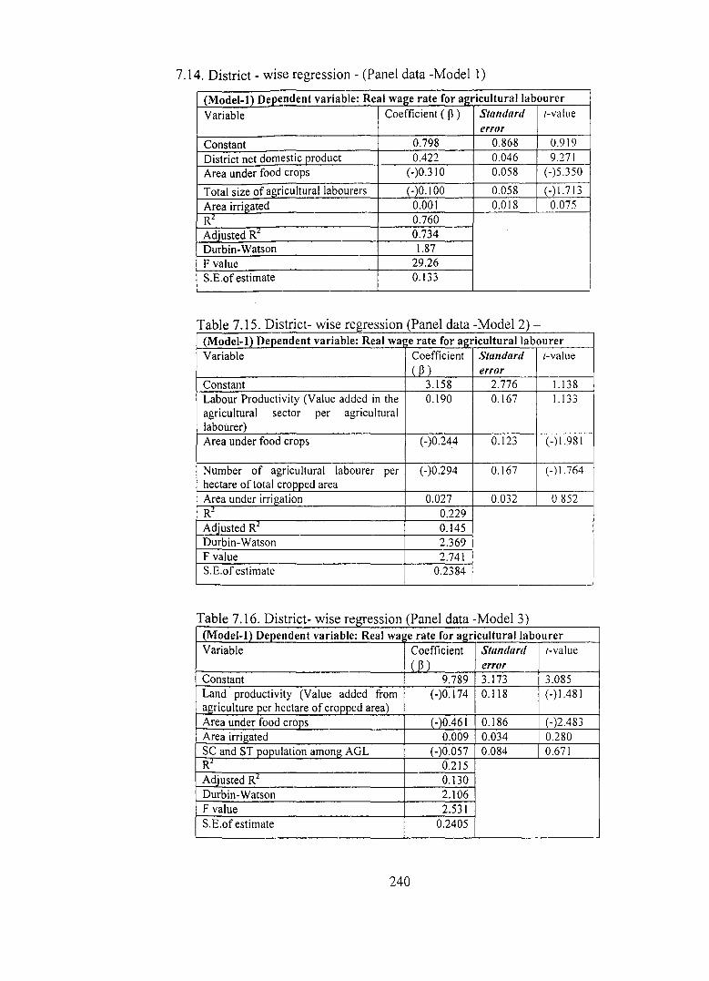
7.14. District- wise regression- (Panel data -Model I)

(Model-l) Dependent variable: Real wage rate for agricultural labourer Variable Coefficient ( p ) Standard /-value

error

Constant 0.798 0.868 0.919

District net domestic product 0.422 0.046 9.271 Area under food crops (-)0.310 0.058 (-)5.350

Total size of agricultural labourers (-)0.1 00 0.058 (-)1.713

Area irrigated 0.001 0.018 0.075 R2 0.760 Adjusted Rl 0.734 Durbin-Watson 1.87 F value 29.26 S.E.of estimate 0.133

T bl 7 15 n· a e Istnct- wise regression (P 1 d M d 12) ane ata- o e -(Model-l) Dependent variable: Real wa e rate for a£riculturallabourer Variable Coefficient Standard !-value

( 13 ) error Constant 3.158 2.776 1.138 Labour Productivity (Value added in the 0.190 0.167 1.133 agricultural sector per agricultural labourer) Area under food crops (-)0.244 0.123 (-)1.981

Number of agricultural labourer per (-)0.294 0.167 (-)1.764 hectare of total cropped area Area under irrigation 0.027 0.032 0.852 R' 0.229 Adjusted Rl 0.145 Durbin-Watson 2.369 F value 2.741 S.E.of estimate 0.2384

T bl 7 16 D' t . t a e IS nc - wise regression (P 1 d t M d 1 3) ane a a- o e (Model-l) Dependent variable: Real wa e rate for agricultural labourer Variable Coefficient Standard /-value

( 13 ) error Constant 9.789 3.173 3.085 Land productivity (Value added from (-)0.174 0.118 (-)1.481 ~iculture per hectare of cropped area) Area under food crops (-)0.461 0.186 (-)2.483 Area irrigated 0.009 0.034 0.280 SC and ST population among AGL (-)0.057 0.084 0.671 R- 0.215 Adjusted Rl 0.130 Durbin-Watson 2.106 F value 2.531 S. E.of estimate 0.2405

240

In other words, the historical component in wage rate is taken into account in

such regressive models. In the present context, one year lagged value of the

dependent variable ln(WiJ-1 is included in the independent variable side. A

result of the regression is presented in Table 7.17. The explanatory power of

the model has increased in the VAR model, but OW is unsatisfactory.

However, the result obtained was not significantly different from the first

model except the fact that the supply side variable specified as the number of

agricultural labourers per hectare of cropped area was found statistically

significant along with the one year lagged values of the real wage rate. It is

important to note that the current year wage rate is significantly influenced by

the wage rate in the previous year.

Table 7.17. District -wise regression (Vector Auto Regressive Model (D d . bl R I fi A . I I L b M epen ent vana e: ea wage rate or .gncu tura a our- en

Variable Coefficient ( p ) t-value Constant 1.904 2.312 District net domestic product at 0.213 I 2.712 constant price I~ Area under food cro_]Js (-)0.257 Real wage rate with one year lag 0.404 ! .., 744

Cropped area per agricuitural (-)0.169 I c-)3.o26 I labourer R· 0.859 Adjusted R- 0.835 Durbin-Watson 1.56 F value 35.080 S.E.of estimate 0.10289

7.4. Conclusion

In this chapter three issues were analysed. Analysis of the secondary

source of data on wage rates of agricultural and other rural labourers revealed

that there were serious lacuna in the wage statistics supplied by the Ministry of

Agriculture in its publication, Agricultural Wages in India. Shortcomings in

the data source was, to a certain extent, resolved by sourcing the data from the

Depm1ment of Economics and Statistics, Government of Kerala. The second

issue dealt with in the chapter was the long term trend in the rate of growth in

real wage, product wage and relative wage. The literature on the trend and

pattern of agricultural wages in India, based on wage data from A WI and

241

NSSO, showed that the real wage rate of agricultural labourers in Kerala

registered a higher growth in the 1990s when compared to 1980s. In sharp

contrast to the observation, the present study, using a variant of the data

published in A WI observed that the rate of growth in real wage rate in the

1990s was lower than the 1980s. Analysis of the trend in the long-run wage

movement indicated that the wage rate in Kerala had experienced different

phases of growth and the growth phases were statistically identified with

structural breaks. Broadly three distinct phases could be identified in the long

run movement of the real wage rate for all categories of labourers except

agricultural labour women. Real wage rate registered a higher growth rate in

the 1960s followed by a slow down in the 1970s. Again, during the 1980s, real

wage rate experienced a higher rate of growth. In the 1990s, real wage slowed

down again. To a great extent, the identified phases of growth in real wage rate

for different categories of rural labourers converged with the phases in area,

production and productivity of impot1ant crops grown in Kerala. The wage

determination model clearly indicated that the short run fluctuations in wage

rates were not related to land or labour productivity as argued by the

marginalist school but the overall development of the region concerned. It in

turn indicated that the wage rate for a particular sector is not determined in

isolation of the developments in allied sectors. However, unlike in other states,

on the demand for labourers and their wage rates, area under irrigation was not

found to have any significant influence. However, real wage rate was observed

to have lower base in regions where the area under food crops was on a higher

side or in other words, an inverse relationship could be observed between real

wage rate and the area under food crops. The vector auto regressive model

showed that the current years wage was a function of last years too, which in

turn indicated that the past struggle and bargaining strength that the labour as a

class could harness did leave its impact on the determination of the wage rate

in the future.

242