Chapter 7: Rapid alignment methods: FASTA and BLAST · Introduction to bioinformatics, Autumn 2007 97 FASTA l FASTA is a multistep algorithm for sequence alignment (Wilbur and Lipman,

Introduction to bioinformatics, Autumn 2007 83

Chapter 7: Rapid alignment methods:FASTA and BLAST

l The biological problem

l Search strategies

l FASTA

l BLAST


The biological problem

• Global and localalignment algoritms areslow in practice

• Consider the scenario ofaligning a querysequence against a largedatabase of sequences– New sequence with

unknown function • For instance, the size of NCBIGenBank in January 2007 was65,369,091,950 bases(61,132,599 sequences)


Problem with large amount ofsequences

l Exponential growth in both number and total length ofsequences

l Possible solution: Compare against model organismsonly

l With large amount of sequences, changes are thatmatches occur by random

− Need for statistical analysis


Application of sequence alignment:shotgun sequencing

l Shotgun sequencing is a method for sequencingwhole-organism genomes

− First, a large number of short sequences (~500-1000 bp), orreads are generated from the genome

− Reads are contiguous subsequences (substrings) of thegenome

− Due to sequencing errors and repetitions in the reads, thegenome has be covered multiple times by reads


Shotgun sequencing

l Ordering of the reads is initially unknown

l Overlaps resolved by aligning the reads

l In a 3x109 bp genome with 500 bp reads and 5x coverage, thereare ~107 reads and ~107(107-1)/2 = ~5x1013 pairwise sequencecomparisons

… …Original genome sequence

ReadsNon-overlappingread

Overlapping reads=> Contig


Shotgun sequencing

l ~5x1013 pairwise sequence comparisonsl Recall that local alignment takes O(nm) time, where n and m are

sequence lengthsl Already with n=m=500, the computation cost is prohibitive

… …Original genome sequence

ReadsNon-overlappingread

Overlapping reads=> Contig


Search strategies

l How to speed up the computation?− Find ways to limit the number of pairwise comparisons

l Compare the sequences at word level to find outcommon words

− Word means here a k-tuple (or a k-word), a substring oflength k


Analyzing the word contentl Example query string I: TGATGATGAAGACATCAG

l For k = 8, the set of k-tuples of I is

TGATGATG

GATGATGA

ATGATGAA

TGATGAAG

…

GACATCAG


Analyzing the word content

l There are n-k+1 k-tuples in a string of length n

l If at least one word of I is not found from another stringJ, we know that I differs from J

l Need to consider statistical significance: I and Jmight share words by chance only

l Let n=|I| and m=|J|


Word lists and comparison by content

l The k-words of I can be arranged into a table of wordoccurences Lw(I)

l Consider the k-words when k=2 and I=GCATCGGC:

GC, CA, AT, TC, CG, GG, GC

AT: 3CA: 2CG: 5GC: 1, 7GG: 6TC: 4

Start indecies of k-word GC in I

Building Lw(I) takes O(n) time


Common k-words

l Number of common k-words in I and J can becomputed using Lw(I) and Lw(J)

l For each word w in I, there are |Lw(J)| occurences in J

l Therefore I and J have

common words

l This can be computed in O(n + m + 4k) time− O(n + m) time to build the lists

− O(4k) time to calculate the sum


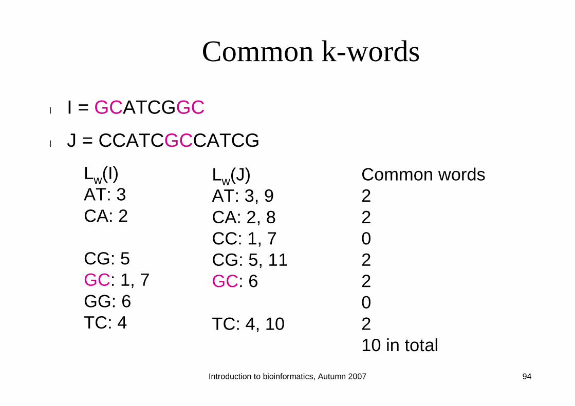
Common k-words

l I = GCATCGGC

l J = CCATCGCCATCG

Lw(J)AT: 3, 9CA: 2, 8CC: 1, 7CG: 5, 11GC: 6

TC: 4, 10

Lw(I)AT: 3CA: 2

CG: 5GC: 1, 7GG: 6TC: 4

Common words220220210 in total


Properties of the common word list

l Exact matches can be found using binary search (e.g., whereTCGT occurs in I?)

− O(log 4k) time

l For large k, the table size is too large to compute the commonword count in the previous fashion

l Instead, an approach based on merge sort can be utilised(details skipped, see course book)

l The common k-word technique can be combined with the localalignment algorithm to yield a rapid alignment approach


Chapter 7: Rapid alignment methods:FASTA and BLAST

l The biological problem

l Search strategies

l FASTA

l BLAST


FASTA

l FASTA is a multistep algorithm for sequence alignment (Wilburand Lipman, 1983)

l The sequence file format used by the FASTA software is widelyused by other sequence analysis software

l Main idea:− Choose regions of the two sequences that look promising (have some

degree of similarity)

− Compute local alignment using dynamic programming in these regions


FASTA outline

l FASTA algorithm has five steps:− 1. Identify common k-words between I and J− 2. Score diagonals with k-word matches, identify 10 best

diagonals− 3. Rescore initial regions with a substitution score matrix− 4. Join initial regions using gaps, penalise for gaps− 5. Perform dynamic programming to find final alignments


Dot matrix comparisonsl Word matches in two sequences I and J can be represented as

a dot matrix

l Dot matrix element (i, j) has ”a dot”, if the word starting atposition i in I is identical to the word starting at position j in J

l The dot matrix can be plotted for various k

i

j

I = … ATCGGATCA …J = … TGGTGTCGC …

i

j


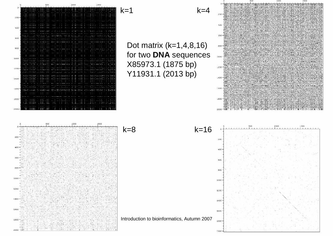
k=1 k=4

k=8 k=16

Dot matrix (k=1,4,8,16)for two DNA sequencesX85973.1 (1875 bp)Y11931.1 (2013 bp)


k=1 k=4

k=8 k=16

Dot matrix(k=1,4,8,16) for twoprotein sequencesCAB51201.1 (531 aa)CAA72681.1 (588 aa)

Shading indicatesnow the match scoreaccording to ascore matrix(Blosum62 here)


Computing diagonal sums

l We would like to find high scoring diagonals of the dot matrix

l Lets index diagonals by the offset, l = i - j

C C A T C G C C A T C GG *C * *A * *T * *C * *GG *C

k=2

I

J

Diagonal l = i – j = -6



l As an example, lets compute diagonal sums for I =GCATCGGC, J = CCATCGCCATCG, k = 2

l 1. Construct k-word list Lw(J)

l 2. Diagonal sums Sl are computed into a table, indexed with theoffset and initialised to zerol -10 -9 -8 -7 -6 -5 -4 -3 -2 -1 0 1 2 3 4 5 6

Sl 0 0 0 0 0 0 0 0 0 0 0 0 0 0 0 0 0



l 3. Go through k-words of I, look for matches in Lw(J) and updatediagonal sums


I

J For the first 2-word in I,GC, LGC(J) = {6}.

We can then updatethe sum of diagonall = i – j = 1 – 6 = -5 toS-5 := S-5 + 1 = 0 + 1 = 1





I

J Next 2-word in I is CA,for which LCA(J) = {2, 8}.

Two diagonal sums areupdated:l = i – j = 2 – 2 = 0S0 := S0 + 1 = 0 + 1 = 1

I = i – j = 2 – 8 = -6S-6 := S-6 + 1 = 0 + 1 = 1





I

J Next 2-word in I is AT,for which LAT(J) = {3, 9}.

Two diagonal sums areupdated:l = i – j = 3 – 3 = 0S0 := S0 + 1 = 1 + 1 = 2

I = i – j = 3 – 9 = -6S-6 := S-6 + 1 = 1 + 1 = 2



After going through the k-words of I, the result is:

l -10 -9 -8 -7 -6 -5 -4 -3 -2 -1 0 1 2 3 4 5 6

Sl 0 0 0 0 4 1 0 0 0 0 4 1 0 0 0 0 0


I

J


Algorithm for computing diagonal sum of scores

Sl := 0 for all 1 – m l n – 1

Compute Lw(J) for all words w

for i := 1 to n – k – 1 do

w := IiIi+1…Ii+k-1

for j Lw(J) do

l := i – j

Sl := Sl + 1

end

end

Match score is here 1


FASTA outline




Rescoring initial regions

l Each high-scoring diagonal chosen in the previous step isrescored according to a score matrix

l This is done to find subregions with identities shorter than k

l Non-matching ends of the diagonal are trimmed

I: C C A T C G C C A T C GJ: C C A A C G C A A T C A

I’: C C A T C G C C A T C GJ’: A C A T C A A A T A A A

75% identity, no 4-word identities

33% identity, one 4-word identity


Joining diagonals

l Two offset diagonals can be joined with a gap, if the resultingalignment has a higher score

l Separate gap open and extension are used

l Find the best-scoring combination of diagonals

High-scoringdiagonals

Two diagonalsjoined by a gap


FASTA outline




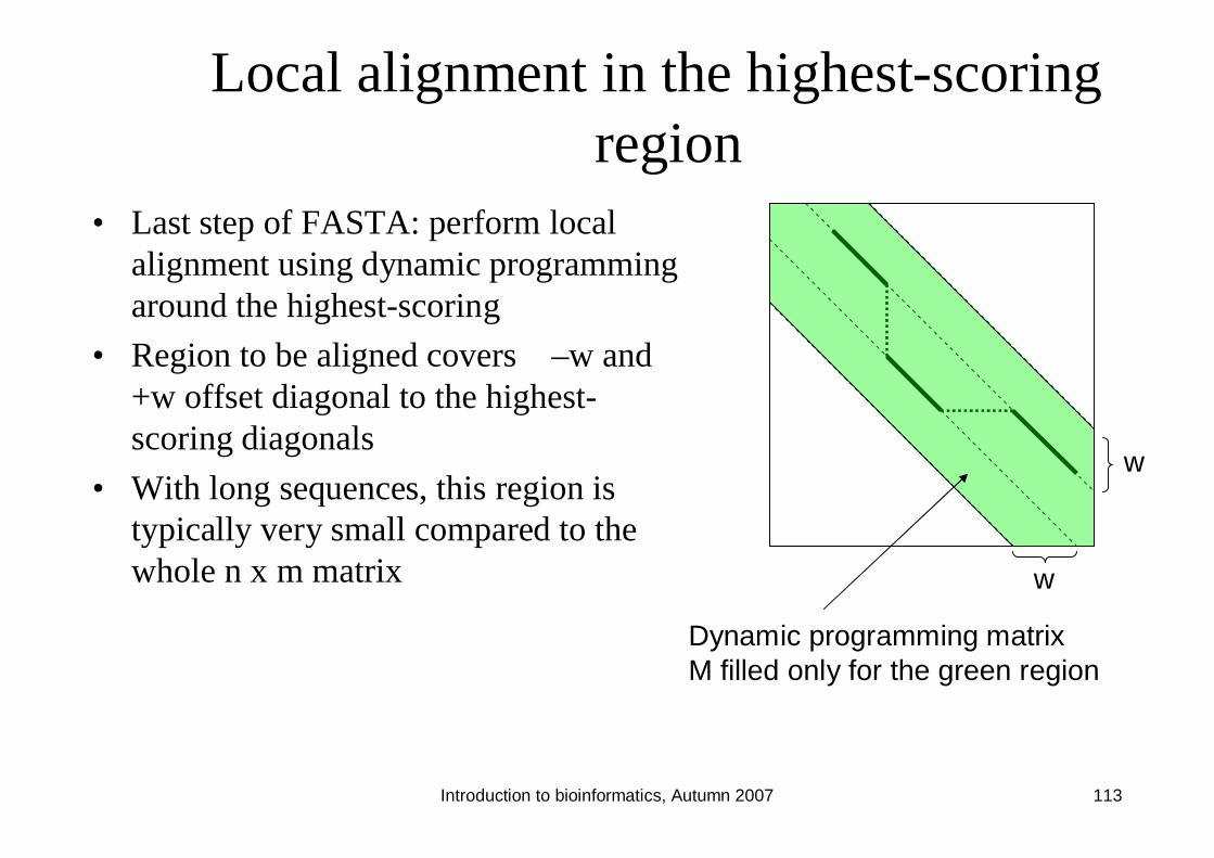
Local alignment in the highest-scoringregion

• Last step of FASTA: perform localalignment using dynamic programmingaround the highest-scoring

• Region to be aligned covers –w and+w offset diagonal to the highest-scoring diagonals

• With long sequences, this region istypically very small compared to thewhole n x m matrix w

w

Dynamic programming matrixM filled only for the green region


Properties of FASTA

l Fast compared to local alignment using dynamic programmingonly

− Only a narrow region of the full matrix is aligned

l Increasing parameter k decreases the number of hits: increasesspecificity, decreases sensitivity

l FASTA can be very specific when identifying long regions oflow similarity

− Specific method does not produce many incorrect results

− Sensitive method produces many of the correct results


Properties of FASTA

l FASTA looks for initial exact matches to querysequence

− Two proteins can have very different amino acid sequencesand still be biologically similar

− This may lead into a lack of sensitivity with divergedsequences


Demonstration of FASTA at EBI

l http://www.ebi.ac.uk/fasta/

l Note that parameter ktup in the software correspondsto parameter k in lectures

http://www.ebi.ac.uk/fasta/

Documents

Chapter 7: Rapid alignment methods: FASTA and BLAST · Introduction to bioinformatics, Autumn 2007 97 FASTA l FASTA is a multistep algorithm for sequence alignment (Wilbur and Lipman,