Chapter 7: Internal Forces - Statics 4300:201 Chap07 - Internal Forces.pdf · where a distributed load begins or ends, and where concentrated forces or concentrated couples are applied

7.1

Chapter 7: Internal Forces

Chapter Objectives

• To show how to use the method of sections for determining the internal

loadings in a member.

• To generalize this procedure by formulating equations that can be plotted so

that they describe the internal shear and moment throughout a member.

In our past discussions on trusses we have considered the internal forces in a

straight two-force member.

• These forces produced only “tension” or “compression” in the member.

• The internal forces in any other type of member will usually produce “shear”

and “bending” as well.

This chapter is devoted to the analysis of the internal forces in “beams.”

• Beams are long, straight prismatic members designed to support loads that are

applied perpendicular to the axis of the member and at various points along the

member.

7.1 Internal Loadings Developed in Structural Members

Consider the case of a straight two-force member.

Cut the member at C.

• To maintain equilibrium an internal

axial force must exist.

Next consider the case of a multi-force member.

• The internal forces in beam AB are

not limited to axial tension or

compression as in the case of

straight two-force members.

• The internal forces also include

“shear” and “bending.”

7.2

By the “method of sections” we can take a cut at any point along the length of

the member to find the internal resisting effects – axial force (P), shear force

(V), and bending moment (M).

• If the entire beam is in

equilibrium, then any portion of

the beam is in equilibrium.

• Equilibrium of the isolated

portion of the beam is achieved

by the internal resisting

effects, where

P – axial force

V – shear force

M – bending moment

Various Types of Loading and Support

A “beam” is a structural member designed to support loads applied at various

points along the member.

• In most cases, the loads are applied perpendicular to the axis of the beam

and will cause only shear and bending.

• However, axial forces may be present in the beam when the applied loads are

not perpendicular to the axis of the beam.

Beams are usually long, straight, and symmetrical (prismatic) in cross section

(such as wide flange sections, commonly called I-beams or W-sections).

• Designing a beam consists essentially in selecting the cross section that will

provide the most effective resistance to bending, shear, and deflection

produced by the applied loads.

The design of a beam includes the following steps.

1. Determine the shear forces and bending moments produced by the applied

loads.

2. Select the best suited cross section.

7.3

A beam may be subjected to various types of applied loads.

Concentrated loads Distributed loads* Both

*Distributed loads may be uniform, trapezoidal, or triangular.

A beam may be supported in a number of ways.

• The distance between the supports, L, is referred to as the “span.”

• The following beams are “statically determinate.”

Simply supported Overhanging Cantilever

• The following beams are “statically indeterminate.”

Continuous Propped cantilever Fixed-Fixed

Free-Body Diagram

The following steps are used to begin the analysis or design of a beam.

• The entire beam is taken as a free-body diagram and the reactions are

determined at the supports.

• Then, to determine the internal forces at any point along the length of the

beam, we cut the beam and draw the free-body diagram of that portion of

the beam.

• Using the three equations of equilibrium we may determine the axial force

(P), shear force (V), and bending moment (M) at any point along the length of

the beam.

7.4

∑ Fx = 0 yields the axial force (P)

∑ Fy = 0 yields the shear force (V)

∑ Mcut = 0 yields the bending moment (M)

Sign Conventions

The following sign conventions are used for the internal effects.

Axial force

Shear force

Bending moment

Methods of analysis

Three methods of analysis will be demonstrated.

• Determining values for shear and bending moment at distinct points on a

beam.

• Writing the equations for shear and bending moment.

• Drawing shear and bending moment diagrams by understanding the

relationships between load, shear, and bending moment.

7.5

Example – Values of Shear and Moment at Specific Locations on a Beam

Given: The beam loaded as shown.

Find: V and M @ x = 0+’, 2’, 4-’, 4+’,

6’, 8-’, 8+’, 10’, and 12-’

x = 0+’

∑ Fy = 0 = 10 – V V = 10 k

∑ Mcut = 0 = - 10 (0) + M M = 0 k-ft

x = 2’

∑ Fy = 0 = 10 – V V = 10 k

∑ Mcut = 0 = - 10 (2) + M M = 20.0 k-ft

x = 4-’

∑ Fy = 0 = 10 – V V = 10 k

∑ Mcut = 0 = - 10 (4) + M M = 40.0 k-ft

x = 4+’

∑ Fy = 0 = 10 – 12 - V V = - 2 k

∑ Mcut = 0 = - 10 (4) + 12 (0) + M

M = 40.0 k-ft

x = 6’

∑ Fy = 0 = 10 – 12 - V V = - 2 k

∑ Mcut = 0 = - 10 (6) + 12 (2) + M

M = 60 – 24 = 36.0 k-ft

7.6

x = 8-’

∑ Fy = 0 = 10 – 12 - V V = - 2 k

∑ Mcut = 0 = - 10 (8) + 12 (4) + M

M = 80 – 48 = 32.0 k-ft

x = 8+’

∑ Fy = 0 = 10 – 12 – 6 - V

V = - 8 k

∑ Mcut = 0 = - 10 (8) + 12 (4)

+ 6 (0) + M

M = 80 – 48 – 0 = 32.0 k-ft

x = 10’

∑ Fy = 0 = 10 – 12 – 6 - V

V = - 8 k

∑ Mcut = 0 = - 10 (10) + 12 (6)

+ 6 (2) + M

M = 100 – 72 – 12 = 16.0 k-ft

x = 12-’

∑ Fy = 0 = 10 – 12 – 6 - V

V = - 8 k

∑ Mcut = 0 = - 10 (12) + 12 (8)

+ 6 (4) + M

M = 120 – 96 – 24 = 0 k-ft

To simplify the calculations, use a free body diagram from the right side.

x = 10’

∑ Fy = 0 = V + 8 V = - 8 k

∑ Mcut = 0 = - M + 8 (2) M = 16.0 k-ft

x = 12-’

∑ Fy = 0 = V + 8 V = - 8 k

∑ Mcut = 0 = - M + 8 (0) M = 0 k-ft

Note: The moment is zero at the supports of simply supported beams.

7.7

Example – Values of Shear and Moment at Specific Locations on a Beam


Find: V and M @ x = 0+’, 3’, 6-’, 6+’,

7.5’, and 9-’

x = 0+’

∑ Fy = 0 = 19 – V V = 19 k

∑ Mcut = 0 = - 19 (0) + M M = 0 k-ft

x = 3’

∑ Fy = 0 = 19 – ½ (6) 3 – ½ (4.5) 3 – V

V = 19 – 9 – 6.75 = 3.25 k

∑ Mcut = 0 = - 19 (3) + ½ (6) 3 (2/3) 3

+ ½ (4.5) 3 (1/3) 3 + M

M = 57 – 18 – 6.75 = 32.25 k-ft

x = 6-’

∑ Fy = 0 = 19 – ½ (6) 6 - ½ (3) 6 – V

V = 19 – 18 – 9 = - 8.0 k

∑ Mcut = 0 = - 19 (6) + ½ (6) 6 (2/3) 6

+ ½ (3) 6 (1/3) 6 + M

M = 114 – 72 – 18 = 24.0 k-ft

x = 6+’

∑ Fy = 0 = V + 8 V = - 8.0 k

∑ Mcut = 0 = - M + 8 (3) M = 24.0 k-ft

7.8

x = 7.5’

∑ Fy = 0 = V + 8 V = - 8.0 k

∑ Mcut = 0 = - M + 8 (1.5) M = 12.0 k-ft

x = 9-’

∑ Fy = 0 = V + 8 V = - 8.0 k

∑ Mcut = 0 = - M + 8 (0) M = 0 k-ft

7.9

7.2 Shear and Moment Equations and Diagrams

The plot of values of shear force and bending moment against a distance “x” are

graphs called “shear and bending moment diagrams.”

• Rather than pick points along a beam and approximate these diagrams by

determining values of shear and bending moment at a limited number of

points, we can write equations to define functions of shear and moment at

any “x” along the beam.

The equations for shear and bending moment may be developed by the following

steps.

• First, determine the number of sets of equations needed to define shear

force and bending moment across the entire length of the beam.

- The shear and bending moment equations will be discontinuous at points

where a distributed load begins or ends, and where concentrated forces

or concentrated couples are applied.

• Next, for each set of equations, draw the necessary free-body diagram.

• Then, for each set of equations, write the equilibrium equations and solve

for shear force (V) and bending moment (M) in terms of position on the

beam (i.e. “x”, where “x” is measured from the left end of the beam).

- Use ∑Fy = 0 to develop the equations for shear force.

- Use ∑Mcut = 0 to develop the equations for the bending moment.

7.10

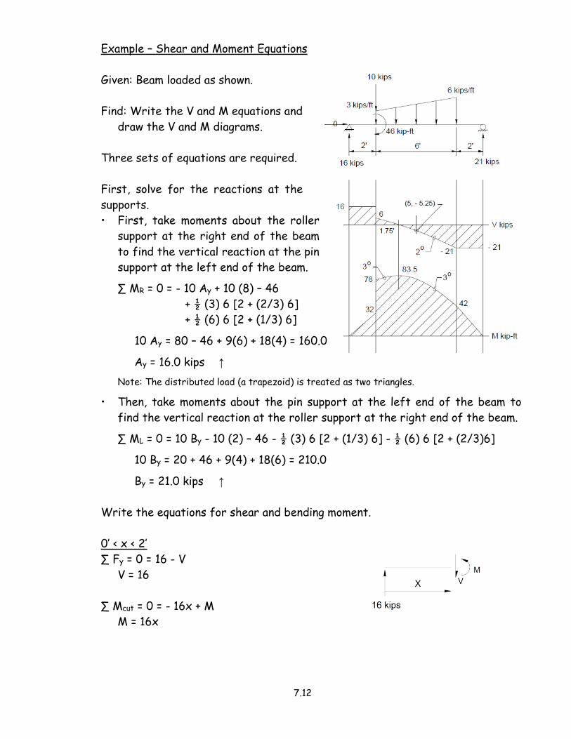
Example – Shear and Moment Equations

Given: Beam loaded as shown.

Find: Write the V and M equations and

draw the V and M diagrams.

Two sets of equations are required.

First, solve for the reactions at the

supports.

∑ MB = 0 = - Ay L + P (L/2)

Ay = P/2

∑ MA = 0 = By L - P (L/2)

By = P/2

Note: The beam is symmetrical and

symmetrically loaded; thus, the

reactions are symmetrical as well.

0 < x < L/2

∑ Fy = 0 = P/2 – V

V = P/2

∑ Mcut = 0 = - (P/2) x + M

M = Px/2

L/2 < x < L

∑ Fy = 0 = P/2 – P - V

V = - P/2

∑ Mcut = 0 = - (P/2) x + P (x – L/2) + M

M = Px/2 – Px + PL/2

M = P/2 (L – x)

7.11





One set of equations is required.

0 < x < L

∑ Fy = 0 = wL/2 – wx - V

V = w (L/2 – x)

∑ Mcut = 0 = - (wL/2) x + wx (x/2) + M

M = - wx2/2 + wLx/2

M = (wx/2) (L – x)

7.12





Three sets of equations are required.

First, solve for the reactions at the

supports.

• First, take moments about the roller

support at the right end of the beam

to find the vertical reaction at the pin

support at the left end of the beam.

∑ MR = 0 = - 10 Ay + 10 (8) – 46

+ ½ (3) 6 [2 + (2/3) 6]

+ ½ (6) 6 [2 + (1/3) 6]

10 Ay = 80 – 46 + 9(6) + 18(4) = 160.0

Ay = 16.0 kips ↑

Note: The distributed load (a trapezoid) is treated as two triangles.

• Then, take moments about the pin support at the left end of the beam to

find the vertical reaction at the roller support at the right end of the beam.

∑ ML = 0 = 10 By - 10 (2) – 46 - ½ (3) 6 [2 + (1/3) 6] - ½ (6) 6 [2 + (2/3)6]

10 By = 20 + 46 + 9(4) + 18(6) = 210.0

By = 21.0 kips ↑

Write the equations for shear and bending moment.

0’ < x < 2’

∑ Fy = 0 = 16 - V

V = 16

∑ Mcut = 0 = - 16x + M

M = 16x

7.13

2’ < x < 8’

Since the intensity of the distributed load

varies, an equation is needed to define the

intensity of the distributed load (p) as a

function of position “x” along the beam.

Using the general equation of a line: p = m x + c

• Determine the slope m.

m = (6 – 3)/(8 – 2) = 1/2

So, p = ½ x + c

• Next, determine the “y-intercept” value “c”.

Known points on the line include: when x = 2, p = 3 and when x = 8, p = 6.

Substituting the second condition into the equation p = ½ x + c:

6 = ½ (8) + c c = 6 – 4 = 2

Thus, p = ½ x + 2

Now write the equations for shear and moment.

∑ Fy = 0 = 16 – 10 – ½ (3) (x – 2) – ½ (½ x + 2) (x – 2) - V

V = 16 – 10 – (3/2) (x – 2) – ½ (½ x + 2) (x – 2)

= 6 – 3x/2 + 3 – ½ (x2/2 + x – 4)

= 6 – 3x/2 + 3 - x2/4 - x/2 + 2

V = - x2/4 – 2x + 11 V = 0 k @ x = 3.75’

∑ Mcut = 0 = - 16x + 10 (x – 2) + ½ (3) (x – 2) (2/3) (x – 2)

+ ½ (½ x + 2) (x – 2) (1/3) (x – 2) + M - 46

M = 16x - 10 (x – 2) - (x – 2)2 – (1/6) (½ x + 2) (x – 2)2 + 46

= 16x – 10x + 20 - (x2 – 4x + 4) – (1/6) (x3/2 – 6x + 8) + 46

= 6x + 20 – x2 + 4x – 4 – x3/12 + x – 1.33 + 46

M = – x3/12 – x2 + 11x + 60.67 M = 83.5 k-ft @ x = 3.75’

8’ < x < 10’

∑ Fy = 0 = V + 21

V = - 21 k

∑ Mcut = 0 = - M + 21 (10 – x)

M = 21 (10 – x)

7.14

7.3 Relations between Distributed Load, Shear, and Moment

The methods outlined so far for drawing shear and bending moment diagrams

become increasingly cumbersome the more complex the loading.

• The construction of shear and bending moment diagrams, however, can

become greatly simplified by understanding the relationships that exist

between the distributed load, the shear force, and the bending moment.

Relation between the Distributed Load and Shear

From the free body diagram:

∑ Fy = 0 = V – (V + ∆V) – w ∆x, where w = w (x) = constant for small ∆x

∆V = – w ∆x

∆V/∆x = - w(x), then letting ∆x → 0, by definition of a derivative,

dV/dx = - w(x)

If we integrate this expression between two points, then

dV = - w(x) dx

∫ dV = - ∫ w(x) dx

V2 – V1 = -∫2

1w(x) dx

Interpretation of these first two expressions:

dV/dx = - w(x) The value of the slope on the shear diagram is

equal to the height of the load diagram at that

point times minus one.

V2 – V1 = -∫2

1w(x) dx The change in shear between two points is equal to

the area under the load diagram times minus one.

Concentrated Forces

These equations are not valid under a concentrated load.

• The shear diagram is discontinuous at the point of a concentrated load.

7.15

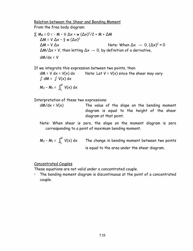
Relation between the Shear and Bending Moment

From the free body diagram:

∑ MR = 0 = - M – V ∆x + w (∆x)2/2 + M + ∆M

∆M = V ∆x – ½ w (∆x)2

∆M = V ∆x Note: When ∆x → 0, (∆x)2 ≈ 0

∆M/∆x = V, then letting ∆x → 0, by definition of a derivative,

dM/dx = V

If we integrate this expression between two points, then

dM = V dx = V(x) dx Note: Let V = V(x) since the shear may vary.

∫ dM = ∫ V(x) dx

M2 – M1 =∫2

1V(x) dx

Interpretation of these two expressions:

dM/dx = V(x) The value of the slope on the bending moment

diagram is equal to the height of the shear

diagram at that point.

Note: When shear is zero, the slope on the moment diagram is zero

corresponding to a point of maximum bending moment.

M2 – M1 =∫2

1V(x) dx The change in bending moment between two points

is equal to the area under the shear diagram.

Concentrated Couples

These equations are not valid under a concentrated couple.

• The bending moment diagram is discontinuous at the point of a concentrated

couple.

7.16

Example – Shear and Moment Diagrams


Find: Draw the shear and moment

diagrams.

Draw the shear diagram

Between the left end and right end of

the beam:

• The area under the load diagram = + wL

∆V = - Area = - wL

V2 = V1 + ∆V

= wL/2 – wL = - wL/2

Draw the moment diagram

Between the left end of the beam and

mid-span:

• The area under the shear diagram

= ½ (wL/2)(L/2) = wL2/8

∆M = Area = wL2/8

M2 = M1 + ∆M

= 0 + wL2/8 = wL2/8

• At mid-span (i.e. x = L/2), V = 0, so dM/dx = 0.

Between mid-span and the right end of the beam:

• The area under the shear diagram = - ½ (wL/2)(L/2) = - wL2/8

∆M = Area = - wL2/8

M2 = M1 + ∆M = wL2/8 + (- wL2/8) = 0

In general, when V = 0 at a point, the slope on the moment diagram at that point

is zero (i.e. a horizontal tangent).

7.17



Find: Draw the shear and moment diagrams.

7.18



Find: Draw the shear and moment diagrams.

7.19




diagrams.

Solve for the reactions at the

supports.

• Take moments about point A to

find the vertical reaction at

point D.

∑MA = 0 = - ½ (4) 12 [(2/3) 12]

– 20 (15) – 120 + 18 Dy

18 Dy = 192 + 300 + 120 = 612.0

Dy = 34.0 k ↑

• Take moments about point D to

find the vertical reaction at

point A.

∑MD = 0 = ½ (4) 12 [6 + (1/3) 12]

+ 20 (3) – 120 - 18 Ay

18 Ay = 240 + 60 - 120 = 180.0

Ay = 10.0 k ↑

In order to draw the first part of the moment diagram, the location for the

point of maximum moment (i.e. V = 0 kips) needs to be determined so that the

area under the shear diagram may be calculated.

• Write an equation for shear between x = 0’ and x = 12’.

∑ Fy = 0 = 10 – ½ (x) (x/3) – V

V = 10 – x2/6

Let V = 0, thus 0 = 10 – x2/6

x2 = 60.0

x = 7.75’

• The change in moment from x = 0’ to x = 7.75’ is equal to the area under the

shear diagram.

Δ M = (2/3) 10 (7.75’) = 51.7 kip-ft

7.20

• Determine the value of moment at x = 12’ and plot this value on the moment

diagram.

- The area under the portion shear diagram between x = 7.75’ and x = 12’

cannot be calculated using standard formulas since there is no horizontal

tangent at x = 7.75’ or at x = 12’.

- Take a cut at x = 12’, draw the

free body diagram, and write the

equilibrium equation to determine

the value of moment.

- Then plot this value on the moment

diagram.

∑ Mcut = 0 = MB – 10 (12) + ½ (12) 4 (1/3)(12)

MB = 120 – 96 = 24.0 kip-ft

The concentrated couple at point C causes the moment diagram to jump up by

120 kip-ft.

• Since the applied moment is acting clockwise, the internal resisting moment

increases, thus the jump “up” on the moment diagram.

7.21




diagrams.

In order to draw the part of the

moment diagram beyond x = 2’, the

location for the point of maximum

moment (i.e. V = 0 kips) needs to be

determined.

• Write an equation for shear for

2’ < x < 8’.

∑ Fy = 0 = 16 - 10 – ½ (3) (x - 2) - ½ (½ x + 2) (x - 2) - V

V = 6 – 3/2 (x – 2) – ½ (½ x + 2) (x – 2)

= 6 – 3x/2 + 3 – ½ (x2/2 + x – 4)

= 6 - 3x/2 + 3 – x2/4 - x/2 + 2

V = - x2/4 – 2x + 11

The maximum moment occurs when V = 0.

• Let V = 0; thus, 0 = - x2/4 – 2x + 11

• Using the quadratic equation, find “x” when V = 0.

x = - (- 2) ± [(- 2 )2 – 4 (- 1/4 ) (11)]1/2

2 (- 1/4)

x = - 11.75’ (Not reasonable: not within the limits of 2’ < x < 8’.)

x = 3.75’

7.22

• Find M @ x = 3.75’

∑ Mcut = 0 = - 16 (3.75) + 10 (1.75) – 46 + ½ (3) 1.75 (2/3) 1.75

+ ½ (3.75/2 + 2) (1.75) (1.75/3) + M

M = 16 (3.75) – 10 (1.75) + 46 – ½ (3) 1.75 (2/3) 1.75

- ½ (3.875) 1.75 (1.75/3)

M = 60 – 17.5 + 46 – 3.06 – 1.98

M = 83.5 k-ft

Documents

Chapter 7: Internal Forces - Statics 4300:201 Chap07 - Internal Forces.pdf · where a distributed load begins or ends, and where concentrated forces or concentrated couples are applied